Physical Mathematics 2010

Dr Peter BoyleSchool of Physics and Astronomy (JCMB 4407)

paboyle@ph.ed.ac.uk

This version: September 20, 2010

AbstractThese are the lecture notes to accompany the Physical Mathematics lecture course. They

are a modified version of the previous years notes which written by Dr Alisdair Hart.

Contents

1 Organisation 51.1 Books . . . . . . . . . . . . . . . . . . . . . . . . . . . . . . . . . . . . . . . . . . . 51.2 On the web . . . . . . . . . . . . . . . . . . . . . . . . . . . . . . . . . . . . . . . . 51.3 Workshops . . . . . . . . . . . . . . . . . . . . . . . . . . . . . . . . . . . . . . . . . 5

2 The wave equation 62.1 Separation of variables . . . . . . . . . . . . . . . . . . . . . . . . . . . . . . . . . . 62.2 Solving the ODE’s . . . . . . . . . . . . . . . . . . . . . . . . . . . . . . . . . . . . 72.3 Boundary and initial conditions . . . . . . . . . . . . . . . . . . . . . . . . . . . . . 7

2.3.1 BCs & orthogonality of normal modes . . . . . . . . . . . . . . . . . . . . . 82.3.2 Completeness of normal modes . . . . . . . . . . . . . . . . . . . . . . . . . 82.3.3 Boundary conditions (in x) . . . . . . . . . . . . . . . . . . . . . . . . . . . . 92.3.4 Normal mode decomposition . . . . . . . . . . . . . . . . . . . . . . . . . . . 102.3.5 Initial conditions (in t) . . . . . . . . . . . . . . . . . . . . . . . . . . . . . . 102.3.6 A quick example . . . . . . . . . . . . . . . . . . . . . . . . . . . . . . . . . 11

3 Fourier Series 123.1 Overview . . . . . . . . . . . . . . . . . . . . . . . . . . . . . . . . . . . . . . . . . . 123.2 The Fourier expansion . . . . . . . . . . . . . . . . . . . . . . . . . . . . . . . . . . 123.3 Orthogonality . . . . . . . . . . . . . . . . . . . . . . . . . . . . . . . . . . . . . . . 133.4 Calculating the Fourier coefficients . . . . . . . . . . . . . . . . . . . . . . . . . . . 133.5 Even and odd expansions . . . . . . . . . . . . . . . . . . . . . . . . . . . . . . . . . 13

3.5.1 Expanding an even function . . . . . . . . . . . . . . . . . . . . . . . . . . . 143.5.2 Expanding an odd function . . . . . . . . . . . . . . . . . . . . . . . . . . . 14

3.6 Periodic extension, or what happens outside the range? . . . . . . . . . . . . . . . . 143.7 Complex Fourier Series . . . . . . . . . . . . . . . . . . . . . . . . . . . . . . . . . . 16

3.7.1 Example . . . . . . . . . . . . . . . . . . . . . . . . . . . . . . . . . . . . . . 173.8 Comparing real and complex Fourier expansions . . . . . . . . . . . . . . . . . . . . 183.9 Differentiation and integration . . . . . . . . . . . . . . . . . . . . . . . . . . . . . . 183.10 Gibbs phenomenon . . . . . . . . . . . . . . . . . . . . . . . . . . . . . . . . . . . . 19

1

4 Functions as vectors 204.1 Linear spaces . . . . . . . . . . . . . . . . . . . . . . . . . . . . . . . . . . . . . . . 20

4.1.1 Gramm-Schmidt orthogonalisation . . . . . . . . . . . . . . . . . . . . . . . 204.1.2 Matrix mechanics . . . . . . . . . . . . . . . . . . . . . . . . . . . . . . . . . 20

4.2 Scalar product of functions . . . . . . . . . . . . . . . . . . . . . . . . . . . . . . . . 204.2.1 Scalar product → integral . . . . . . . . . . . . . . . . . . . . . . . . . . . . 21

4.3 Inner products, orthogonality, orthonormality and Fourier series . . . . . . . . . . . 214.3.1 Example: complex Fourier series . . . . . . . . . . . . . . . . . . . . . . . . . 224.3.2 Normalised basis functions . . . . . . . . . . . . . . . . . . . . . . . . . . . . 23

5 Fourier transforms 245.0.3 Relation to Fourier Series . . . . . . . . . . . . . . . . . . . . . . . . . . . . 245.0.4 FT conventions . . . . . . . . . . . . . . . . . . . . . . . . . . . . . . . . . . 24

5.1 Some simple examples of FTs . . . . . . . . . . . . . . . . . . . . . . . . . . . . . . 245.1.1 The top-hat . . . . . . . . . . . . . . . . . . . . . . . . . . . . . . . . . . . . 24

5.2 The Gaussian . . . . . . . . . . . . . . . . . . . . . . . . . . . . . . . . . . . . . . . 265.2.1 Gaussian integral . . . . . . . . . . . . . . . . . . . . . . . . . . . . . . . . . 265.2.2 Fourier transform of Gaussian . . . . . . . . . . . . . . . . . . . . . . . . . . 27

5.3 Reciprocal relations between a function and its F.T . . . . . . . . . . . . . . . . . . 285.4 FTs as generalised Fourier series . . . . . . . . . . . . . . . . . . . . . . . . . . . . . 295.5 Differentiating Fourier transforms . . . . . . . . . . . . . . . . . . . . . . . . . . . . 305.6 The Dirac delta function . . . . . . . . . . . . . . . . . . . . . . . . . . . . . . . . . 30

5.6.1 Definition . . . . . . . . . . . . . . . . . . . . . . . . . . . . . . . . . . . . . 305.6.2 Sifting property . . . . . . . . . . . . . . . . . . . . . . . . . . . . . . . . . . 315.6.3 The delta function as a limiting case . . . . . . . . . . . . . . . . . . . . . . 315.6.4 Proving the sifting property . . . . . . . . . . . . . . . . . . . . . . . . . . . 315.6.5 Some other properties of the Dirac function . . . . . . . . . . . . . . . . . . 325.6.6 FT and integral representation of δ(x) . . . . . . . . . . . . . . . . . . . . . 32

5.7 Convolution . . . . . . . . . . . . . . . . . . . . . . . . . . . . . . . . . . . . . . . . 335.7.1 Examples of convolution . . . . . . . . . . . . . . . . . . . . . . . . . . . . . 34

5.8 The convolution theorem . . . . . . . . . . . . . . . . . . . . . . . . . . . . . . . . . 345.8.1 Examples of the convolution theorem . . . . . . . . . . . . . . . . . . . . . . 35

5.9 Physical applications of Fourier transforms . . . . . . . . . . . . . . . . . . . . . . . 355.9.1 Far-field optical diffraction patterns . . . . . . . . . . . . . . . . . . . . . . . 35

2

1 Organisation

Online notes & tutorial sheets

www.ph.ed.ac.uk/~paboyle/Teaching/PhysicalMathematics/

1.1 Books

There are many books covering the material in this course. Good ones include:

• “Mathematical Methods for Physics and Engineering”, K.F. Riley, M.P. Hobson and S.J. Bence(Cambridge University Press)

– The main textbook.

– Available at a discount from the Teaching Office.

• “Mathematical Methods in the Physical Sciences”, M.L. Boas (Wiley)

• “Mathematical Methods for Physicists”, G. Arfken (Academic Press)

These, and plenty more besides, are available for free in the JCMB library.

1.2 On the web

There are some useful websites for quick reference, including:

• http://mathworld.wolfram.com,

• http://en.wikipedia.org,

• http://planetmath.org.

1.3 Workshops

Workshops run from week 2 through week 11.Sign up for one of the two sessions at Teaching Office:

• Tuesday 11:10-12:00 (room 1206C JCMB)

• Tuesday 14:00-15:50 (room 3217 JCMB)

In week 11, I will set a 60 minute mock exam, then for the final 60 minutes answers will bedistributed and you will mark your neighbours script (or your own if you prefer).The mark will not contribute to your course mark, but serves as useful practice and diagnostic.

3

2 The wave equation

We can the transverse displacement of a stretched string using a function u(x, t) which tells us howfar the infinitesimal element of string at (longitudinal) position x has been (transversely) displacedat time t. The function u(x, t) satisfies a partial differential equation (PDE) known as the waveequation:

∂2u

∂x2=

1

c2∂2u

∂t2(2.1)

where c is a constant,and has units of length over time (i.e. of velocity) and is, in fact, the speed ofpropagation of travelling waves on the string.In the absence of boundaries, the general solution can be seen by noting:

∂2u

∂x2− 1

c2∂2u

∂t2=

(∂

∂x− 1

c

∂

∂t

)(∂

∂x+

1

c

∂

∂t

)u

=

(∂

∂x+

1

c

∂

∂t

)(∂

∂x− 1

c

∂

∂t

)u

This is solved byu(x, t) = f(x− ct) + g(x+ ct)

where f and g are arbitrary functions of a single variable. This represents the superposition ofarbitrary left and right propagating waves.

2.1 Separation of variables

Our equation of motion in Eqn. (2.1) is perhaps the simplest second order partial differential equa-tion (PDE) imaginable – it doesn’t contain any mixed derivatives (e.g. ∂2u

∂x∂t). We call such a

differential equation a separable one, or say that it is of separable form.We can seek particular solutions in which variations with space and time are independent. Such arestanding waves of the of the seperable form:

u(x, t) = X(x) T (t) .

This really is a restriction of the class of possible solutions and there are certainly solutions to thewave equation that are not of separated form (e.g. travelling waves as above).However, we shall see all solutions of the wave equation (separated form or not) can be written asa linear combination of solutions of separated form, so this restriction is not a problem.Differentiating, we get

∂u

∂x=dX

dxT ≡ X ′T ⇒ ∂2u

∂x2= X ′′T

∂u

∂t=X

dT

dt≡ XT ⇒ ∂2u

∂t2= XT

Substituting this into the PDE:

X ′′(x)T (t) =1

c2X(x)T (t) ,

Thus,X(x)′′

X(x)=

1

c2T (t)

T (t)

4

Now∂

∂tLHS =

∂

∂xRHS = 0

Hence both LHS and RHS must be equal to the same constant and we may write

X ′′

X=

1

c2T

T= −k2 (say),

where −k2 is called the separation constant.

EXAM TIP: You will lose marks here if you do not write “Seeking solutions of separated form”,and explain something equivalent to the above discussion.Now we have separated our PDE in two variables into two simple second order ordinary differentialequations (ODEs) in one variable each:

d2X

dx2=− k2X(x)

d2T

dt2=− ω2

kT (t)

where the angular frequency ωk = ck. This is the interpretation of c for standing waves: it is theconstant of proportionality that links the wavenumber k to the angular frequency ωk.These have the form of an eigenvalue problem, where X(x) must be an eigenfunction of d2

dx2 with

eigenvalue −k2. Similarly T (t) must be an eigenfunction of d2

dt2with eigenvalue −ω2

k = −c2k2.

2.2 Solving the ODE’s

We can now solve the two ODEs separately. The solutions to these are familiar from simple harmonicmotion, and we can just write down the solutions:

X(x) =Ak sin kx+Bk cos kx

T (t) =Ck sinωkt+Dk cosωkt

⇒ u(x, t) = (Ak sin kx+Bk cos kx) (Ck sinωkt+Dk cosωkt)

where Ak, Bk, Ck, and Dk are arbitrary constants. The subscript denotes that they can takedifferent values for different values of k. At this stage there is no restriction on the values of k: eachvalues provides a separate solution to the ODEs.Note that a propagating wave, of the form

cos (kx− ωkt) = cos kx cosωkt+ sin kx sinωkt

and so a propagating wave can be written as a linear combination of standing waves.

2.3 Boundary and initial conditions

The details of a specific physical system may involve the boundary conditions (BCs) solutions mustsatisfy. For example, what happens at the ends of the string and what were the initial conditions.The string weight & tension on a guitar determine c.The length (& frets) of a guitar determine the boundary conditions.The plucking of the guitar determines the initial conditions.

5

2.3.1 BCs & orthogonality of normal modes

Physicists tend to be somewhat lazy (or perhaps unclear?) about decomposing general functionsinto eigenfunctions of a given differential operator.Sturm–Liouville theory describes a class of problem and gives some useful results. We will notgo into a complete discussion of Sturm-Liouville problems, but note that the ODE equations weconsider in this course in fact satisfy the Sturm-Liouville conditions. We summarise some of theprecise statements made possible.Suppose X1 and X2 are eigenfunctions of d2

dx2 , with eigenvalues −λ1 and −λ2, and satisfy some BCsat x = a and x = b.

X1 = −λ1X1

X2 = −λ2X2

Observe:d

dx(X1X2 −X1X2) = X1X2 −X1X2

Thus,

b∫a

(X1X2 −X1X2

)dx =

[X1X2 −X1X2

]ba

= (λ2 − λ1)

b∫a

X1X2dx (2.2)

Now, for many standard boundary conditions the Wronskian[X1X2 −X1X2

]ba

= 0, for example:

Dirichlet X1(a) = X1(b) = X2(a) = X2(b) = 0

Neumann X1(a) = X1(b) = X2(a) = X2(b) = 0

Periodic X1(a) = X1(b) ; X2(a) = X2(b) ;X1(a) = X1(b) ;X2(a) = X2(b)

In these boundary conditions, eigenfunctions with distinct eigenvalues are orthogonal under thescalar (dot) product defined by:

X1 ·X2 =

b∫a

X1X2dx

If λ1 = λ2, then we are not guaranteed orthogonality, however, if X1 and X2 are genuinely different(linearly independent) then the Gramm-Schmidt procedure in section 4.1 allows us to construct anorthonormal basis in any case.

2.3.2 Completeness of normal modes

Proof of completeness is beyond the scope of this course. However, we can state two theoremsregarding different meanings of “completeness”:

6

Uniform convergence:

if a function f has continuous first and second derivatives on [a, b] and f satisfies the boundaryconditions then f can be exactly represented by a sum of eigenmodes: it will match at every point.That is the maximum deviation between f(x) and the sum S(x) =

∑n

anXn of eigenmodes becomes

zero as the number of modes included tends to ∞.

maxx∈a,b

|f(x)− S(x)|2;→ 0 (2.3)

Any solution of the differential equation satisfying the boundary conditions can be written as a sumof eigenmodes.

L2 convergence:

If the function f(x) hasb∫a

|f(x)|2dx finite it can be approximated by a sum S(x) =∑n

anXn of

eigenmodes in the weaker senseb∫

a

|f(x)− S(x)|2dx→ 0 (2.4)

(2.4) means that the sum S(x) can deviate from f(x) at certain points, and the maximum errorcan remain non-zero. However, not for anything other than an inifinitessimal distance asotherwiseit would contribute something to the integral.Thus the basis is complete it can describe and only differs infinitessimally close to discontinuitiesand violations of the boundary conditions.

any bounded function on the interval [a, b] can be described away from discontinuities & boundaries

2.3.3 Boundary conditions (in x)

Consider the guitar example above.Assume the string is stretched between x = 0 and x = L, then the BCs in this case are thatu(x = 0, t) = u(x = L, t) = 0 for all t. Because these BCs hold for all times at specific x, they affectX(x) rather than T (t). We find

u(0, t) = 0 ⇒ Bk = 0 ,

u(L, t) = 0 ⇒ kn = nπ/L , n = 0, 1, 2 . . .

Here, BCs have restricted the allowed values of k and thus the allowed frequencies of oscillation.Different boundary conditions will have different allowed values. Restriction of eigenvalues byboundary conditions is a very general property in physics:

finite boundaries ⇒ discrete (quantised) eigenvalue spectrum.

Each n value corresponds to a normal mode of the string:

u(x, t) = An sin knx{Cn sinωnt+Dn cosωnt}

A normal mode is an excitation of the string that obeys the BCs and oscillates with a single, normalmode frequency. We sometimes call these eigenmodes of the system, with associated eigenfrequenciesωn = ωkn .

7

2.3.4 Normal mode decomposition

Just like any vector can be represented as a linear combination of basis vectors, so the generalsolution to the wave equation is a linear superposition of (normal) eigenmode solutions:

u(x, t) =∞∑n=1

An sin knx{Cn sinωnt+Dn cosωnt}

≡∞∑n=1

sin knx{En sinωnt+ Fn cosωnt} (2.5)

As before ωn = ckn. We sum only from n = 1 because sin k0x = 0, and we do not need to includenegative n because sin −nπx

L= − sin nπx

L. Constants An, Cn, Dn are all unknown, so we can merge

them together to give En = AnCn and Fn = AnDn.We also see that the way we have ensured that u(0, t) = 0 is by making it an odd function in x:u(−x, t) = −u(x, t) ⇒ u(0, t) = 0.

2.3.5 Initial conditions (in t)

As we have a second order temporal ODE, we need two sets of initial conditions to solve the problem.Typically these are the the shape f(x) and velocity profile g(x) of the string at t = 0:

u(x, 0) = f(x) =∞∑n=1

Fn sin knx

u(x, 0) = g(x) =∞∑n=1

ωnEn sin knx

These conditions determine unique values for each of the En and Fn. Having got these, we cansubstitute them back into the general solution to obtain u(x, t) and thus describing the motion forall times.Consider the equation for Fn. Let’s choose to calculate one, specific constant out of this set i.e. Fmfor some specific m. To do this, multiply both sides by sin kmx and integrate over the whole string(in this case x = 0...L) giving:∫ L

0

dx f(x) sin kmx =∞∑n=1

Fn

∫ L

0

dx sin knx sin kmx .

Now we note that the sine functions form an orthogonal set :∫ L

0

dx sin knx sin kmx =1

2

∫ L

0

dx [cos(knx− kmx)− cos(knx+ kmx)]

=1

2

[

sin(knx−kmx)kn−km

− sin(knx+kmx)kn+km

]L0

; n 6= m[x− sin(knx+kmx)

kn+km

]L0

; n = m

=L

2δmn

8

where δmn is the Kronecker delta, giving zero for m 6= n So:∫ L

0

dx f(x) sin kmx =∞∑n=1

Fn

∫ L

0

dx sin knx sin kmx

=L

2

∞∑n=1

Fnδmn

=L

2Fm

using the sifting property. Therefore, after relabelling m→ n:

Fn =2

L

∫ L

0

dx f(x) sin knx

En =2

Lωn

∫ L

0

dx g(x) sin knx . (2.6)

We are given f and g, so as long as we can do the integrals on the RHS, we have determined allthe unknown constants and therefore know the motion for all times.The solution written as a sum of sine waves is an example of a Fourier series.

2.3.6 A quick example

Suppose the initial conditions are that the string is initially stretched into a sine wave f(x) =a sin(3πx/L) (for some a) and at rest, i.e. g(x) = 0.The latter immediately gives En = 0 for all n. The former gives:

Fn =2

L

∫ L

0

dx f(x) sin knx

=2a

L

∫ L

0

dx sin3πx

Lsin

nπx

L=

2a

L× L

2δn3

using the above relation. So all the Fn are zero except F3 = a. So the motion is described by

u(x, t) = a sin3πx

Lcos

3πct

L.

The answer is very simple. If the system starts as a pure normal mode of the system, it will remainas one.

9

3 Fourier Series

3.1 Overview

Fourier series are a way of decomposing a function as a sum of sine and cosine waves. We candecompose almost any function in this way as discussed in section 2.3.2Fourier serieas are particularly useful if we are looking at system that satisfies a wave equation,because sinusoids are the normal mode oscillations which have simple time dependence. We canuse this decomposition to understand more complicated excitations of the system.Fourier series describe a finite interval of a function, typically −L→ L or 0 → L. If the size of thesystem is infinite we instead need to use Fourier transforms which we will learn later in Sec. 5.Outside this range a Fourier series is periodic (repeats itself) because all the sine and cosine wavesare themselves periodic. The Fourier series periodically extends the function outside the range.Fourier series are useful in the following contexts:

• The function really is periodic e.g. a continuous square wave

• We are only interested in what happens inside the expansion range.

Fourier modes Consider the wave equation on an interval [−L,L] with periodic boundary con-ditions

d2X(x)

dx2= −k2X(x)

X(x+ 2L) = X(x)

The solutions look like

X(x) = akψk(x) + bkφk(x) ,

where ψk(x) ≡ cos kx ,

φk(x) ≡ sin kx .

ak, bk are unknown constants. Now, periodicity condition means cos k(x + 2L) = cos kx andsin k(x+ 2L) = sin kx. This is satisfied if 2kL = 2nπ or

k =nπ

Lfor n an integer.

3.2 The Fourier expansion

The set of Fourier modes {ψn≥0(x), φn≥1(x)} are therefore defined as:

ψn(x) = cosnπx

L,

φn(x) = sinnπx

L(3.1)

Between −L ≤ x ≥ L we can write a general real function as a linear combination of these Fouriermodes:

f(x) =∞∑n=0

anψn(x) +∞∑n=1

bnφn(x)

= a0 +∞∑n=1

(anψn(x) + bnφn(x)) (3.2)

where an and bn are (real-valued) Fourier coefficients.

10

3.3 Orthogonality

Having written a function as a sum of Fourier modes, we would like to be able to calculate thecomponents. This is made easy because the Fourier mode functions are orthogonal i.e.∫ L

−Ldx ψm(x)ψn(x) = Nψ

n δmn ,∫ L

−Ldx φm(x)φn(x) = Nφ

n δmn ,∫ L

−Ldx ψm(x)φn(x) = 0 .

Nψn≥0 and Nφ

n≥1 are normalisation constants which we find by doing the integrals using the trig.identities in Eqn. (3.3) below. It turns out that Nψ

n = Nφn = L for all n, except n = 0 when

Nψ0 = 2L.

ASIDE: useful trig. relation To prove the orthogonality, the following double angle formulaeare useful:

2 cosA cosB = cos(A+B) + cos(A−B)

2 sinA cosB = sin(A+B) + sin(A−B)

2 sinA sinB = − cos(A+B) + cos(A−B)

2 cosA sinB = sin(A+B)− sin(A−B) (3.3)

3.4 Calculating the Fourier coefficients

The orthogonality proved above allows us to calculate the Fourier coefficients as follows:

am =

1

2L

∫ L

−Ldx ψm(x)f(x) m = 0 ,

1

L

∫ L

−Ldx ψm(x)f(x) m > 0 ,

Similarly, bm =1

L

∫ L

−Ldx φm(x)f(x) .

Proof: suppose f(x) =∑

k akψk + bkφk, then

1

Nψj

∫ L

−Lψjf(x)dx =

∑k

ak

Nψj

∫ L

−Lψk +

bk

Nψj

∫ L

−Lφkdx

=∑k

akδjk + bk × 0

= aj

The proof for bk is very similar.

3.5 Even and odd expansions

What if the function we wish to expand is even:f(−x) = f(x), or odd: f(−x) = −f(x)? Becausethe Fourier modes are also even (ψn(x)) or odd (φn(x)), we can simplify the Fourier expansions.

11

3.5.1 Expanding an even function

Consider first the case that f(x) is even:

bm =1

L

∫ L

−Ldx φm(x)f(x) =

1

L

∫ L

0

dx φm(x)f(x) +1

L

∫ 0

−Ldx φm(x)f(x)

In the second integral, make a change of variables y = −x⇒ dy = −dx. The limits on y are L→ 0,and use this minus sign to switch them round to 0 → L. f(x) = f(−y) = +f(y) because it is aneven function, whereas φm(x) = φm(−y) = −φm(y) as it is odd. Overall, then:

bm =1

L

∫ L

0

dx φm(x)f(x)− 1

L

∫ L

0

dy φm(y)f(y) = 0

i.e. the Fourier decomposition of an even function contains only even Fourier modes. Similarly, wecan show that

am =1

L

∫ L

0

dx ψm(x)f(x) +1

L

∫ L

0

dy ψm(y)f(y) =2

L

∫ L

0

dx ψm(x)f(x)

for m > 0 and

a0 =1

L

∫ L

0

dx ψm=0(x)f(x) .

3.5.2 Expanding an odd function

For an odd function we get a similar result: all the am vanish, so we only get odd Fourier modes,and we can calculate the bm by doubling the result from integrating from 0 → L:

am = 0

bm =2

L

∫ L

0

dx φm(x)f(x)

We derive these results as before: split the integral into regions of positive and negative x; makea transformation y = −x for the latter; exploit the symmetries of f(x) and the Fourier modesψm(x), φm(x).

3.6 Periodic extension, or what happens outside the range?

We call the original function f(x), possibly defined for all x, and the Fourier series expansion fFS(x).Inside the expansion range fFS(x) is guaranteed to agree exactly with f(x). Outside this range,the Fourier expansion fFS(x) need not, in general, agree with f(x) which is after all an arbitraryfunction.Consider function f(x) = x2 between −L and L. This is an even function so we know bn = 0. Theother coefficients are:

a0 =1

2L

∫ L

−Ldx x2 =

1

L

∫ L

0

dx x2 =1

L

L3

3=L2

3

We need to do the integral

am =2

L

∫ L

0

dx x2 cosmπx

L

12

x

f(x)=x 2

π 3π−π−3π

Figure 3.1: f(x) = x2 as a periodic function.

The first stage is to make a substitution that simplifies the argument of the cosine function:

y =mπx

L⇒ dy =

mπ

Ldx

which also changes the upper integration limit to mπ. So

am =2

L

∫ mπ

0

L

nπdy

L2y2

m2π2cos y =

2L2

m3π3

∫ mπ

0

dy y2 cos y .

We now solve this simplified integral by integrating by parts. An easy way of remembering integra-tion by parts is ∫

u.dv = uv −∫v.du

and in this case we will make u = y2 and dv = cos y. Because y2 is an integer power, repeatdifferentiation will eventually yield a constant and we can do the integral.∫

dy y2 cos y = y2 sin y −∫dy 2y sin y .

We now repeat the process for the integral on the RHS, setting u = 2y for the same reason:∫dy y2 cos y = y2 sin y −

[−2y cos y +

∫dy 2 cos y

]= y2 sin y + 2y cos y − 2 sin y .

So, using sinmπ = 0 and cosmπ = (−1)m:

am =2L2

m3π3

[y2 sin y + 2y cos y − 2 sin y

]mπ0

=2L2

m3π3× 2mπ(−1)m =

4L2(−1)m

m2π2(3.4)

So, overall our Fourier series is

fFS(x) =L2

3+

4L2

π2

∞∑n=1

(−1)n

n2cos

nπx

L. (3.5)

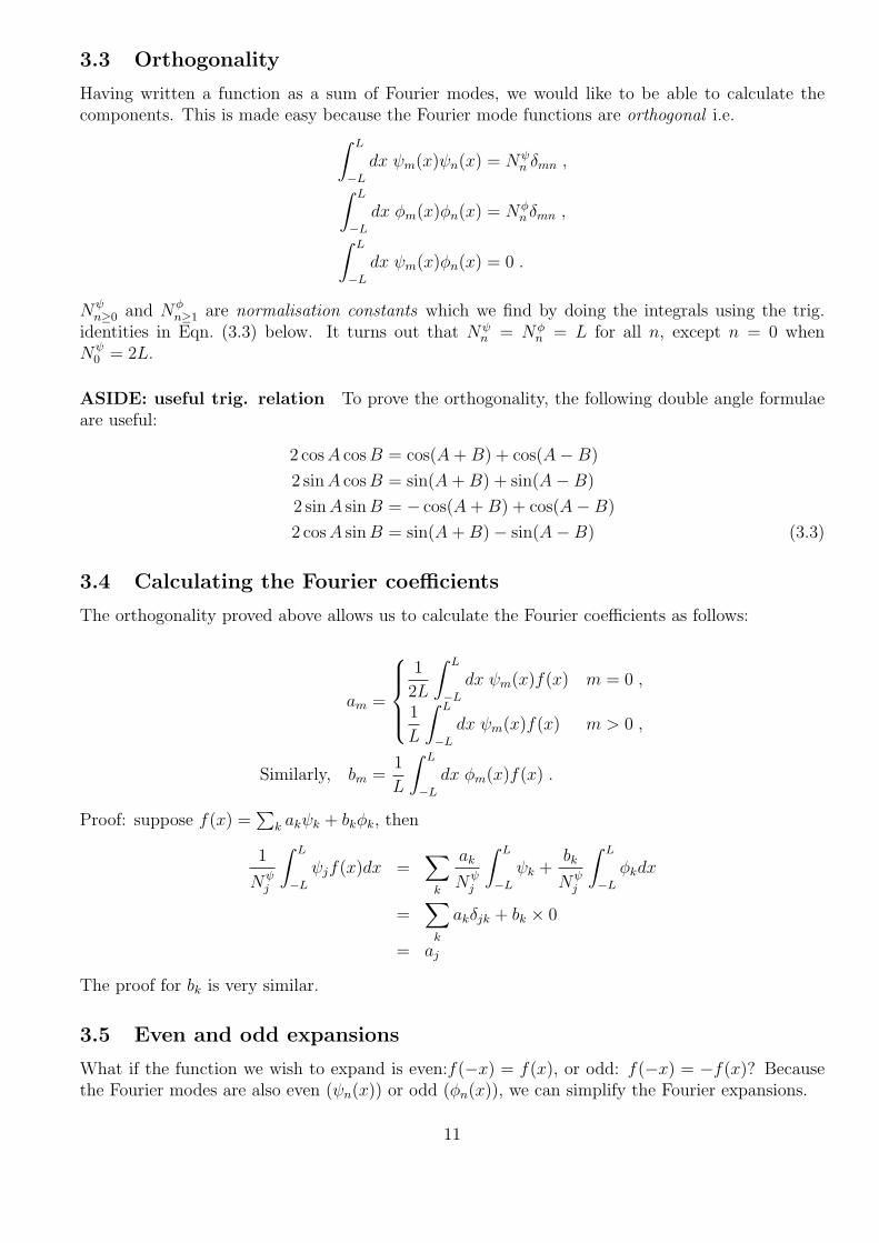
fFS(x) agrees exactly with the original function f(x) inside the expansion range. Outside, howeverin general it need not. The Fourier series has periodically extended the function f(x) outside theexpansion range, Fig. 3.1. Only if f(x) itself has the same periodicity will fFS(x) agree with f(x)for all x.A plot of the coefficients, {cn} versus n, is known as the spectrum of the function: it tells us howmuch of each frequency is present in the function. The process of obtaining the coefficients is oftenknown as spectral analysis. We show the spectrum for f(x) = x2 in Fig. 3.2.

13

Figure 3.2: The Fourier spectrum an (with y-axis in units of L2) for function f(x) = x2.

3.7 Complex Fourier Series

Sines and cosines are one Fourier basis i.e. they provide one way to expand a function in the interval[−L,L]. Another, related basis is that of complex exponentials.

f(x) =∞∑

n=−∞

cnϕn(x) where ϕn(x) = e−iknx = e−inπx/L (3.6)

This is a complex Fourier series, because the expansion coefficients, cn, are in general complexnumbers even for a real-valued function f(x) (rather than being purely real as before). Note thatthe sum over n runs from −∞ in this case.These basis functions are also orthogonal and the orthogonality relation in this case is

∫ L

−Ldx ϕ∗m(x)ϕn(x) =

∫ L

−Ldx ei(km−kn)x =

[x]L−L = 2L (if n = m)[exp(i(km−kn)x)

i(km−kn)

]L−L

= 0 (if n 6= m)

= 2L δmn

Note the complex conjugation of ϕm(x). For the case n 6= m, we note that m − n is a non-zerointeger (call it p) and

exp[i(km−kn)L]−exp[i(km−kn)(−L)] = exp[ipπ]−exp[−ipπ] = (exp[iπ])p−(exp[−iπ])p = (−1)p−(−1)p = 0 .

For p = m− n = 0 the denominator is also zero, hence the different result.We can use (and need) this orthogonality to find the coefficients. If we decide we want to calculatecm for some chosen value of m, we multiply both sides by the complex conjugate of ϕm(x) and

14

integrate over the full range:∫ L

−Ldx ϕm(x)∗f(x) =

∞∑n=−∞

cn

∫ L

−Ldx ϕm(x)∗ϕn(x) =

∞∑n=−∞

cn.2Lδmn = cm.2L

⇒ cm =1

2L

∫ L

−Ldx ϕm(x)∗f(x) =

1

2L

∫ L

−Ldx eikmxf(x)

As before, the integral of a sum is the same as a sum of integrals, that cn are constants.

3.7.1 Example

Go back to our example of expanding f(x) = x2 for x ∈ [−L,L] (we could choose L = π if wewished).We decide to calculate component cm for a particular value of m, which involves an integral asabove. In fact, we can generalise and calculate all the different m values using two integrals: onefor m = 0 and another for generic m 6= 0:

cm=0 =1

2L

∫ L

−Ldx x2 =

L2

3

cm6=0 =1

2L

∫ L

−Ldx x2e−imπx/L =

2L2(−1)m

2m2π2

See below for details of how to do the second integral. We notice that in this case all the cm arereal, but this is not the case in general.

ASIDE: doing the integral We want to calculate

cm ≡1

2L

∫ L

−Ldx x2eimπx/L

To make life easy, we should change variables to make the exponent more simple (whilst keeping yreal) i.e. set y = mπx/L, for which dy = dx.mπ/L. The integration limits become ±mπ:

cm =1

2L

∫ mπ

−mπdy

L

mπ× L2y2

m2π2eiy =

L2

2m3π3

∫ mπ

−mπdy y2eiy

Again we integrate by parts. We set u = y2 ⇒ du = 2y and dv = eiy ⇒ v = eiy/i = −ieiy. So

cm =L2

2m3π3

{[−iy2eiy

]mπ−mπ −

∫ mπ

−mπdy 2y.(−i)eiy

}=

L2

2m3π3

{[−iy2eiy

]mπ−mπ + 2i

∫ mπ

−mπdy yeiy

}Repeating, this time with u = y ⇒ du = 1 to get:

cm =L2

2m3π3

{[−iy2eiy

]mπ−mπ + 2i

([−iyeiy

]mπ−mπ −

∫ mπ

−mπdy (−i)eiy

)}=

L2

2m3π3

{[−iy2eiy

]mπ−mπ + 2i

([−iyeiy

]mπ−mπ + i

[−ieiy

]mπ−mπ

)}=

L2

2m3π3

[−iy2eiy − 2i.i.yeiy + 2i.i.(−i).eiy

]mπ−mπ

=L2

2m3π3

[−iy2eiy + 2yeiy + 2ieiy

]mπ−mπ

15

We can now just substitute the limits in, using eimπ = e−imπ = (−1)m. Alternately, we can notethat the first and third terms are even under y → −y and therefore we will get zero when weevaluate between symmetric limits y = ±mπ (N.B. this argument only works for symmetric limits).Only the second term, which is odd, contributes:

cm =L2

2m3π3

[2yeiy

]mπ−mπ =

L2

2m3π3

(2mπe−imπ − (−2mπ)eimπ

)=

L2

2m3π3× 4mπ(−1)m =

2L2(−1)m

m2π2(3.7)

3.8 Comparing real and complex Fourier expansions

There is a strong link between the real and complex Fourier basis functions, because cosine andsine can be written as the sum and difference of two complex exponentials:

ϕn(x) = ψn(x)− iφn(x) ⇒

ψn(x) =

1

2[ϕ−n(x) + ϕn(x)]

φn(x) =1

2i[ϕ−n(x)− ϕn(x)]

so we expect there to be a close relationship between the real and complex Fourier coefficients.Staying with the example of f(x) = x2, we can rearrange the complex Fourier series by splittingthe sum as follows:

fFS(x) = c0 +∞∑n=1

cne−inπx/L +

−∞∑n=−1

cneinπx/L

we can now relabel the second sum in terms of n′ = −n:

fFS(x) = c0 +∞∑n=1

cne−inπx/L +

∞∑n′=1

c−n′ein′πx/L

Now n and n′ are just dummy summation indices with no external meaning, so we can now relabeln′ → n and the second sum now looks a lot like the first. Noting from Eqn. (3.7) that in this casec−m = cm, we see that the two sums combine to give:

fFS(x) = c0 +∞∑n=1

cn (ϕn(x) + ϕ−n(x)) = c0ψ0 +∞∑n=1

2cnψn(x)

So, this suggests that our real and complex Fourier expansions are identical with a0 = c0 andan>0 = 2cn>0 (and bn = 0). Comparing our two sets of coefficients in Eqns. (3.4) and (3.7), we seethis is true.

3.9 Differentiation and integration

If the Fourier series of f(x) is differentiated or integrated, term by term, the new series is the Fourierseries for f ′(x) or

∫dx f(x), respectively. This means that we do not have to do a second expansion

to, for instance, get a Fourier series for the derivative of a function.

16

Figure 3.3: The Gibbs phenomenon for truncated Fourier approximations to the signum functionEqn. 3.8. Note the different x-range in the lower two panels.

3.10 Gibbs phenomenon

An interesting case is when we try to describe a function with a finite discontinuity (i.e. a jump)using a truncated Fourier series. Consider the signum function which picks out the sign of a variable:

f(x) = signum x =

{−1 if x < 0 ,

+1 if x ≥ 0 ,(3.8)

We saw in section 2.3.2 that the Fourier series will describe only guarantee to describe a discontin-uous function in the sense of the integrated mean-square difference tending to zero as the numberof terms included is increased.In Fig. 3.3 we plot the original function f(x) and the truncated Fourier series fn(x) for variousnumbers of terms N in the series. We find that the truncated sum works well, except near thediscontinuity. Here the function overshoots the true value and then has a “damped oscillation”.As we increase N the oscillating region gets smaller, but the overshoot determining the maximumdeviation remains roughly the same size (about 18%).The average error decreases to zero, however, because the width of the overshoot shrinks to zero.Thus deviations between fN(x) and f(x) can be large, and is concentrated at those certain valuesof x where the discontinuity in f(x) lies.Note that for any finite number of terms fn(x) must be continuous, because it is a sum of a finitenumber of continuous functions. Describing discontinuities is naturally challenging.The overshoot is known as the Gibbs phenomenon or as a “ringing artefact”. For the interested,there are some more details at http://en.wikipedia.org/wiki/Gibbs phenomenon.

17

4 Functions as vectors

4.1 Linear spaces

Formally, both unit vectors and eigenfunctions can be used to form linear spaces.That is given a set of things {vi}, a linear space is formed by taking all possible linear combinationsof these things. This set of all linear combinations is the span of {vi}.The things could be unit vectors in the coordinate axes for vectors (the ak are coordinates), orequally well, the eigenfunctions of a differential equation, and the ak are Fourier coefficients.Providing the addition of things follows simple axioms such as:

(aivi) + (bjvj) = (ai + bi)vi

and there is a well defined scalar product we can infer quite a lot.We call {vi} linearly independent if

aivi = 0 ⇒ ai = 0.

If this is the case, then none of the vi can be written as a linear combination of the others.(If a set of vectors span the linear space but are not linearly independent, we can reduce the size ofthe set until we do have a linearly independent set that spans the space. The size of this reducedset is the dimension d of the space.)

4.1.1 Gramm-Schmidt orthogonalisation

We now consider make use of the dot product. We can normalise the first vector as e0 = 1|v0|v0.

We can orthogonalise all the d− 1 other vectors with respect to e0

v′i = vi − (vi · e0)e0.

As the vectors are linearly independent, v′i must be non-zero, and we can normalise v′1 to form e1.The process can now be repeated to eliminate components parallel to e1 from the d−2 other vectors.When this process terminates there will be d orthonormal basis vectors, and thus an orthonormalbasis for a linear space can always be found.

4.1.2 Matrix mechanics

In the early days of quantum mechanics Heisenberg worked on matrix mechanics, while Schroedingerworked with the wavefunctions solving his equation.The relation between the two is actually simple and relevant here. Heisenberg described a quantumstate as a state vector of coefficients describing the linear combination of eigenfunctions. Thus wasa coordinate in the linear space spanned by the eigenfunctions.Heisenberg operators were then matrices which acted on these vectors.

4.2 Scalar product of functions

In physics we often make the transition:

discrete picture → continuous picture.

Take N particles of mass m = MN

evenly spaced on a massless string of length L, under tension T .The transverse displacement of the nth particle is un(t). As there are N coordinates we can thinkof the motion as occurring in an N -dimensional space.The gap between particles is a = L/(N + 1), and we can label the nth particle with x = xn ≡ na.We can also write un(t), the transverse displacement of the nth particle, as u(xn, t).

18

a a a a

mm

m m

mm m

0 L

x

u u u1 2 3 45 6

Nuuu

u

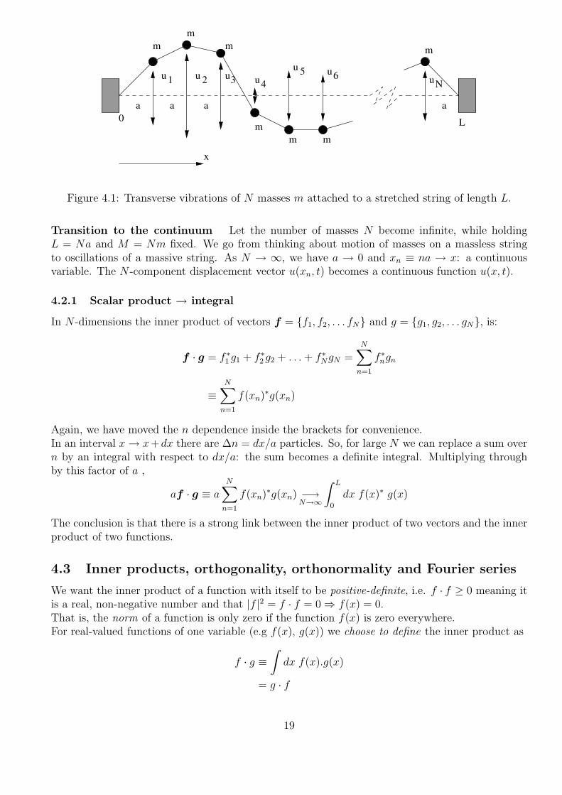
Figure 4.1: Transverse vibrations of N masses m attached to a stretched string of length L.

Transition to the continuum Let the number of masses N become infinite, while holdingL = Na and M = Nm fixed. We go from thinking about motion of masses on a massless stringto oscillations of a massive string. As N → ∞, we have a → 0 and xn ≡ na → x: a continuousvariable. The N -component displacement vector u(xn, t) becomes a continuous function u(x, t).

4.2.1 Scalar product → integral

In N -dimensions the inner product of vectors f = {f1, f2, . . . fN} and g = {g1, g2, . . . gN}, is:

f · g = f ∗1 g1 + f ∗2 g2 + . . .+ f ∗NgN =N∑n=1

f ∗ngn

≡N∑n=1

f(xn)∗g(xn)

Again, we have moved the n dependence inside the brackets for convenience.In an interval x→ x+dx there are ∆n = dx/a particles. So, for large N we can replace a sum overn by an integral with respect to dx/a: the sum becomes a definite integral. Multiplying throughby this factor of a ,

af · g ≡ aN∑n=1

f(xn)∗g(xn) −→

N→∞

∫ L

0

dx f(x)∗ g(x)

The conclusion is that there is a strong link between the inner product of two vectors and the innerproduct of two functions.

4.3 Inner products, orthogonality, orthonormality and Fourier series

We want the inner product of a function with itself to be positive-definite, i.e. f · f ≥ 0 meaning itis a real, non-negative number and that |f |2 = f · f = 0 ⇒ f(x) = 0.That is, the norm of a function is only zero if the function f(x) is zero everywhere.For real-valued functions of one variable (e.g f(x), g(x)) we choose to define the inner product as

f · g ≡∫dx f(x).g(x)

= g · f

19

and for complex-valued functions

f · g ≡∫dx f(x)∗.g(x)

= (g · f)∗ 6= g · f

The integration limits are chosen according to the problem we are studying. For Fourier analysiswe use −L→ L. For the special case of waves on a string we used 0 → L.

Normalised: We say a function is normalised if the inner product of the function with itself is1, i.e. if f · f = 1.

Orthogonal: We say that two functions are orthogonal if their inner product is zero, i.e. iff · g = 0. If we have a set of functions for which any pair of functions are orthogonal, we call it anorthogonal set, i.e. if φm · φn ∝ δmn for all m, n.

Orthonormal: If all the functions in an orthogonal set are normalised, we call it an orthonormalset i.e. if φm · φn = δmn.

4.3.1 Example: complex Fourier series

An example of an orthogonal set is the set of complex Fourier modes {ϕn}. We define the innerproduct as

f · g =

∫ L

−Ldx f(x)∗g(x)

and we see the orthogonality:

ϕm · ϕn ≡∫ L

−Ldx ϕm(x)∗ϕn(x) = Nn δmn

with normalisation Nn ≡ ϕn · ϕn = 2L. This makes for a handy notation for writing down theFourier component calculations that we looked at before:

f(x) =∞∑

n=−∞

cnϕn(x) ⇒ cn =ϕn · fϕn · ϕn

In more detail, the numerator is

ϕn · f ≡∫ L

−Ldx ϕ∗n(x)f(x)

Note that the order of the functions is very important : the basis function comes first.In each case, we can projected out the relevant Fourier component by exploiting the fact that thebasis functions formed an orthogonal set. The same can be done for the real Fourier series whichwe leave as an exercise.

20

4.3.2 Normalised basis functions

Consider the complex Fourier series. If we define some new functions

ϕn(x) ≡1

√ϕn · ϕn

ϕn(x) =ϕn(x)√

2L

then it should be clear thatϕm · ϕn = δmn

giving us an orthonormal set. The inner product is defined exactly as before.We can choose to use these normalised functions as a Fourier basis, with new expansion coefficientsCn:

f(x) =∞∑

n=−∞

Cnϕn(x) ⇒ Cn = ϕn · f

because the denominator ϕn · ϕn = 1.Coefficients Cn and cn are closely related:

Cn = ϕn · f =ϕn · f√ϕn · ϕn

=√ϕn · ϕn

ϕn · fϕn · ϕn

=√ϕn · ϕn cn =

√2L cn

We can do the same for real Fourier series, defining ψn and φn and associated Fourier coefficientsAn and Bn. The relationship to an and bn can be worked out in exactly the same way.

21

5 Fourier transforms

Fourier transforms (FTs) are an extension of Fourier series that can be used to describe functionson an infinite interval. A function f(x) and its Fourier transform F (k) are related by:

F (k) =1√2π

∫ ∞

−∞dx f(x) eikx , (5.1)

f(x) =1√2π

∫ ∞

−∞dk F (k) e−ikx . (5.2)

We say that F (k) is the FT of f(x), and that f(x) is the inverse FT of F (k).FTs include all wavenumbers −∞ < k <∞ rather than just a discrete set.

EXAM TIP: If you are asked to state the relation between a function and it’s Fourier transform(for maybe 3 or 4 marks), it is sufficient to quote these two equations. If they want you to repeatthe derivation in Sec. 5.4, they will ask explicitly for it.

5.0.3 Relation to Fourier Series

Fourier series only include modes with kn = 2nπL

. This constraint on k arose from imposing period-icity on the eigenfunctions of the wave equation. Adjacent modes were separated by δk = 2π

L.

Now, as L→∞, δk → 0 and the Fourier Series turns into the Fourier Transform.We’ll show this in more detail in Sec. 5.4.

5.0.4 FT conventions

Eqns. (5.1) and (5.2) are the definitions we will use for FTs throughout this course. Unfortunately,there are many different conventions in active use for FTs. These can differ in:

• The sign in the exponent

• The placing of the 2π prefactor(s)

• Whether there is a factor of 2π in the exponent

You will probably come across different conventions at some point in your career and it is importantto always check and match conventions.

5.1 Some simple examples of FTs

In this section we’ll find the FTs of some simple functions.

EXAM TIP: Looking at past papers, you are very often asked to define and sketch f(x) in eachcase, and also to calculate and sketch F (k).

5.1.1 The top-hat

A top-hat function Π(x) of height h and width 2a (a assumed positive), centred at x = d is definedby:

Π(x) =

{h, if d− a < x < d+ a ,

0, otherwise .(5.3)

22

The function is sketched in Fig. 5.1.Its FT is:

F (k) =1√2π

∫ ∞

−∞dx Π(x) eikx =

h√2π

∫ d+a

d−adx eikx =

√2a2h2

πeikd sinc ka (5.4)

The derivation is given below. The function sinc x ≡ sinxx

is sketched in Fig. 5.2 (with notes on howto do this also given below). F (k) will look the same (for d = 0), but the nodes (zeros) will now be

at k = ±nπa

and the intercept will be√

2a2h2

πrather than 1. You are very unlikely to have to sketch

F (k) for d 6= 0.

Deriving the FT:

F (k) =1√2π

∫ ∞

−∞dx Π(x) eikx =

h√2π

∫ d+a

d−adx eikx

Now we make a substitution u = x−d (which now centres the top-hat at u = 0), and have du = dx..The integration limits become u = ±a. This gives

F (k) =h√2π

· eikd∫ a

−adu eiku =

h√2π

· eikd[eiku

ik

]a−a

=h√2π

· eikd(eika − e−ika

ik

)=

h√2π

· eikd · 2a

ka· e

ika − e−ika

2i=

√4a2h2

2π· eikd · sin ka

ka=

√2a2h2

πeikd sinc ka

Note that we conveniently multiplied top and bottom by 2a midway through.

Sketching sincx: You should think of sinc x ≡ sinxx

as a sinx oscillation (with nodes at x = ±nπfor integer n), but with the amplitude of the oscillations dying off as 1/x. Note that sincx is aneven function, so it is symmetric when we reflect about the y-axis.The only complication is at x = 0, when sinc 0 = 0

0which appears undefined. Instead of thinking

about x = 0, we should think about the limit x→ 0 and use l’Hopital’s Rule (see below):

limx→0

sinc x = limx→0

[ddx

sin xddxx

]= lim

x→0

[cosx

1

]= 1

The final sketch is given in Fig. 5.2.

Figure 5.1: Sketch of top-hat function defined in Eqn. (5.3)

23

EXAM TIP: Make sure you can sketch this, and that you label all the zeros and intercepts.

Revision: l’Hopital’s Rule: If (and only if!) f(x) = g(x) = 0 for two functions at some valuex = c, then

limx→c

[f(x)

g(x)

]= lim

x→c

[f ′(x)

g′(x)

], (5.5)

where primes denote derivatives. Note that we differentiate the top and bottom separately ratherthan treating it as a single fraction.If (and only if!) both f ′(x = c) = g′(x = c) = 0 as well, we can repeat this to look at doublederivatives and so on. . .

5.2 The Gaussian

The Gaussian curve is also known as the bell-shaped or normal curve. A Gaussian of width σcentred at x = d is defined by:

f(x) = N exp

(− x2

2σ2

)(5.6)

where N is a normalisation constant, which is often set to 1. We can instead define the normalisedGaussian, where we choose N so that the area under the curve to be unity i.e. N = 1/

√2πσ2

(derived below).

5.2.1 Gaussian integral

Gaussian integrals occur regularly in physics. We are interested in

I =

∫ ∞

−∞exp−x2dx

Figure 5.2: Sketch of sinc x ≡ sinxx

24

This can be solved via a trick in polar coordinates: observe

I2 =

∫ ∞

−∞exp−x2dx

∫ ∞

−∞exp−y2dy

=

∫ ∞

−∞dx

∫ ∞

−∞dy exp−(x2 + y2)

=

∫ ∞

0

dr2πr exp−r2

= π

∫ ∞

0

du exp−u

= π [− exp−u]∞0= π

Thus,

I =

∫ ∞

−∞exp−x2dx =

√π

5.2.2 Fourier transform of Gaussian

The Gaussian is sketched for two different values of the width parameter σ. Fig. 5.3 has N = 1in each case, whereas Fig. 5.4 shows normalised curves. Note the difference, particularly in theintercepts.The FT is

F (k) =1√2π

∫ ∞

−∞dx N exp

(− x2

2σ2

)eikx = Nσ exp

(−k

2σ2

2

), (5.7)

i.e. the FT of a Gaussian is another Gaussian (this time as a function of k).

Deriving the FT For notational convenience, let’s write a = 12σ2 , so

F (k) =N√2π

∫ ∞

−∞dx exp

(−[ax2 − ikx

])

Figure 5.3: Sketch of Gaussians with N = 1

25

Now we can complete the square inside [. . .]:

−ax2 + ikx = −(x√a− ik

2√a

)2

− k2

4a

giving

F (k) =N√2πe−k

2/4a

∫ ∞

−∞dx exp

(−[x√a− ik

2√a

]2).

We then make a change of variables:

u = x√a− ik

2√a.

This does not change the limits on the integral, and the scale factor is dx = du/√a, giving

F (k) =N√2πa

e−k2/4a

∫ ∞

−∞du e−u

2

= N

√1

2a· e−k2/4a .

Finally, we change back from a to σ.

5.3 Reciprocal relations between a function and its F.T

These examples illustrate a general and very important property of FTs: there is a reciprocal (i.e.inverse) relationship between the width of a function and the width of its Fourier transform. Thatis, narrow functions have wide FTs and wide functions have narrow FTs.This important property goes by various names in various physical contexts, e.g.:

• Uncertainty principle: the width of the wavefunction in position space (∆x) and the width ofthe wavefunction in momentum space (∆p) are inversely related: ∆x ·∆p ' h.

• Bandwidth theorem: to create a very short-lived pulse (small ∆t), you need to include a verywide range of frequencies (large ∆ω).

• In optics, this means that big objects (big relative to wavelength of light) cast sharp shadows(narrow F.T. implies closely spaced maxima and minima in the interference fringes).

We discuss some explicit examples:

Figure 5.4: Sketch of normalised Gaussians. The intercepts are f(0) = 1√2πσ2

.

26

The top-hat: The width of the top-hat as defined in Eqn. (5.3) is obviously 2a.For the FT, whilst the sinc ka function extends across all k, it dies away in amplitude, so it doeshave a width. Exactly how we define the width does not matter; let’s say it is the distance betweenthe first nodes k = ±π/a in each direction, giving a width of 2π/a.Thus the width of the function is proportional to a, and the width of the FT is proportional to 1/a.

The Gaussian: Again, the Gaussian extends infinitely but dies away, so we can define a width.Choosing a suitable definition, the width of f(x) is σ (other definitions will differ by a numericalfactor).Comparing the form of FT in Eqn. (5.7) to the original definition of the Gaussian in Eqn. (5.6), ifthe width of f(x) is σ, the width of F (k) is 1/σ by the same definition.Again, we have a reciprocal relationship between the width of the function and that of its FT.

The “spike” function: We shall see in section 5.6.6 that the extreme case of an infinitely narrowspike has an infinitely broad (i.e. constant as a function of k) Fourier transform.

5.4 FTs as generalised Fourier series

As we mentioned above, FTs are the natural extensions of Fourier Series that are used to describefunctions in an infinite interval rather than one of size L or 2L.We know that any function f(x) defined on the interval −L < x < L can be represented by acomplex Fourier series

f(x) =∞∑

n=−∞

Cne−iknx, (5.8)

where the coefficients are given by

Cn =1

2L

∫ L

−Ldx f(x) eiknx . (5.9)

where the allowed wavenumbers are k = nπL

. Now we want to investigate what happens if we let Ltend to infinity.At finite L, the separation of adjacent wavenumbers (i.e. for n → n + 1) is δk = π

L. As L → ∞,

δk → 0.Now we do a common trick in mathematical physics and multiply both sides of Eqn. (5.8) by 1. Thetrick is that we just multiply by 1 on the LHS, but on the RHS we exploit the fact that Lδk/π = 1and multiply by that instead:

f(x) =∞∑

n=−∞

δk

(L

πCn

)e−iknx . (5.10)

Now, what is the RHS? It is the sum of the areas of a set of small rectangular strips of width δk andheight

(LπCn)e−iknx. As we take the limit L→∞ and δk tends to zero, we have exactly defined an

integral rather than a sum:∑

n δk →∫dk. The wavenumber kn becomes a continuous variable k

and Cn becomes a function C(k).For convenience, let’s define a new function:

F (k) =√

2π × limL→∞

(L

πCn

)and Eqn. (5.10) becomes the FT as defined in Eqn. (5.2).

27

For the inverse FT, we multiply both sides of Eqn. (5.9) by Lπ×√

2π:

√2π

(L

π

)Cn =

1√2π

∫ L

−Ldx f(x) eiknx . (5.11)

The limit L → ∞ is more straightforward here: kn → k and the LHS becomes F (k). This is thenexactly the inverse FT defined in Eqn. (5.1).

EXAM TIP: You are often asked to explain how the FT is the limit of a Fourier Series (forperhaps 6 or 7 marks), so make sure you can reproduce the stuff in this section.

5.5 Differentiating Fourier transforms

As we shall see, F.T.s are very useful in solving PDEs. This is because the F.T. of a differential isrelated to the F.T F (k) of the original function by a factor of ik. It is simple to show by replacingf(x) with the the inverse F.T. of F(k):

f ′(x) =d

dx

1√2π

∫ ∞

−∞F (k)e−ikx =

1√2π

∫ ∞

−∞(−ik)F (k)e−ikx,

and in general:

f (p)(x) =1√2π

∫ ∞

−∞(−ik)pF (k)e−ikx. (5.12)

5.6 The Dirac delta function

The Dirac delta function is a very useful tool in physics, as it can be used to represent somethingvery localised or instantaneous which retains a measurable total effect. It is easier to think of itas an infinitely narrow (and tall) spike, and defining it necessarily involves a limiting process suchthat it is “narrower” than “anything else”.

5.6.1 Definition

The Dirac delta function δ(x− d) is defined by two expressions. First, it is zero everywhere exceptat the point x = d where it is infinite:

δ(x− d) =

{0 for x 6= d ,

→∞ for x = d .(5.13)

Secondly, it tends to infinity at x = d in such a way that the area under the Dirac delta function isunity: ∫ ∞

−∞dx δ(x− d) = 1 . (5.14)

i.e. if the integration range contains the spike we get 1, otherwise we get 0. In many cases theupper and lower limits are infinite (a = −∞, b = ∞) and then we always get 1.

EXAM TIP: When asked to define the Dirac delta function (maybe for 3 or 4 marks), makesure you write both Eqns. (5.13) and (5.14).

28

5.6.2 Sifting property

The sifting property of the Dirac delta function is that, given some function f(x):∫ ∞

−∞dx δ(x− d) f(x) = f(d) (5.15)

i.e. the delta function picks out the value of the function at the position of the spike (so long as itis within the integration range).Of course, the integration limits don’t technically need to be infinite in the above formulæ. If weintegrate over a finite range a < x < b the expressions become:∫ b

a

dx δ(x− d) f(x) =

{f(d) for a < d < b ,

0 otherwise.

That is, we get the above results if the position of the spike is inside the integration range, and zerootherwise.

EXAM TIP: If you are asked to state the sifting property, it is sufficient to write Eqn. (5.15).You do not need to prove the result as in Sec. 5.6.4 unless they specifically ask you to.

5.6.3 The delta function as a limiting case

It is sometimes hard to work with the delta function directly and it is easier to think of it as thelimit of a more familiar function. The exact shape of this function doesn’t matter, except that itshould look more and more like a (normalised) spike as we make it narrower.Two possibilities are the top-hat as the width a → 0 (normalised so that h = 1/(2a)), or thenormalised Gaussian as σ → 0. We’ll use the top-hat here, just because the integrals are easier.Let Πa(x) be a normalised top-hat of width 2a centred at x = 0 as in Eqn. (5.3) — we’ve made thewidth parameter obvious by putting it as a subscript here. The Dirac delta function can then bedefined as

δ(x) = lima→0

Πa(x) . (5.16)

5.6.4 Proving the sifting property

We can use the limit definition of the Dirac delta function [Eqn. (5.16)] to prove the sifting propertygiven in Eqn. (5.15):∫ ∞

−∞dx f(x) δ(x) =

∫ ∞

−∞dx f(x) lim

a→0Πa(x) = lim

a→0

∫ ∞

−∞dx f(x) Πa(x) .

Substituting for Πa(x), the integral is only non-zero between −a and a.∫ ∞

−∞dx f(x) δ(x) = lim

a→0

1

2a

∫ a

−adx f(x) .

Now, f(x) is an arbitrary function so we can’t do much more. Except that we know we are goingto make a small, so we can Taylor expand the function around x = 0 (i.e. the position of the centreof the spike) knowing this will be a good description of the function for small enough a:∫ ∞

−∞dx f(x) δ(x) = lim

a→0

1

2a

∫ a

−adx

[f(0) + xf ′(0) +

x2

2!f ′′(0) + . . .

].

29

The advantage of this is that all the f (n)(0) are constants, which makes the integral easy:∫ ∞

−∞dx f(x) δ(x) = lim

a→0

1

2a

(f(0) [x]a−a + f ′(0)

[x2

2

]a−a

+f ′′(0)

2!

[x3

3

]a−a

+ . . .

)= lim

a→0

(f(0) +

a2

6f ′′(0) + . . .

)= f(0) .

which gives the sifting result.

EXAM TIP: It is a common exam question to ask you to derive the sifting property in this way.Make sure you can do it.Note that the odd terms vanished after integration. This is special to the case of the spike beingcentred at x = 0. It is a useful exercise to see what happens if the spike is centred at x = d instead.

5.6.5 Some other properties of the Dirac function

These include:

δ(−x) = δ(x)

δ(ax) =δ(x)

|a|

δ(x2 − a2) =δ(x− a) + δ(x+ a)

2|a|(5.17)

For the last two observe: ∫ ∞

−∞f(x)δ(ax)dx =

∫ ∞

−∞f(

u

|a|)δ(u)

du

|a|=f(0)

|a|

and

δ(x2 − a2) = δ([x− a][x+ a]) = δ([x− a]2a) + δ(−2a[x+ a]) =δ([x− a]) + δ([x+ a])

2|a|

5.6.6 FT and integral representation of δ(x)

The Dirac delta function is very useful when we are doing FTs. The FT of the delta function followseasily from the sifting property:

F (k) =1√2π

∫ ∞

−∞dx δ(x− d) eikx =

eikd√2π

.

In the special case d = 0, we get F (k) = 1/√

2π.

Extreme case reciprocal relation:

F.T. of infinitely narrow spike is infinitely broad

30

f

g

xx’

h(x)

h=f*g*

Figure 5.5: Illustration of the convolution of two functions.

The inverse FT gives us the integral representation of the delta function:

δ(x− d) =1√2π

∫ ∞

−∞dk F (k)e−ikx =

1√2π

∫ ∞

−∞dk

(eikd√2π

)e−ikx

=1

2π

∫ ∞

−∞dk e−ik(x−d) .

∫∞−∞ dk e−ik(x) = 2πδ(x)

Note the prefactor of 2π rather than√

2π.In the same way that we have defined a delta function in x, we can also define a delta functionin k. This would, for instance, represent a signal composed of oscillations of a single frequency orwavenumber K.

5.7 Convolution

Convolution combines two (or more) functions in a way that is useful for describing physical systems(as we shall see). A particular benefit of this is that the FT of the convolution is easy to calculate.The convolution of two functions f(x) and g(x) is defined to be

f(x) ∗ g(x) =

∫ ∞

−∞dx′ f(x′)g(x− x′) ,

The result is also a function of x, meaning that we get a different number for the convolution foreach possible x value. Note the positions of the dummy variable x′ (a common mistake in exams).We can interpret the convolution process graphically. Imagine we have two functions f(x) andg(x) each positioned at the origin. By “positioned” we mean that they both have some distinctivefeature that is located at x = 0. To convolve the functions for a given value of x:

1. On a graph with x′ on the horizontal axis, sketch f(x′) positioned (as before) at x′ = 0,

2. Sketch g(x′), but displaced to be positioned at x′ = x,

3. Flip the sketch of g(x′) left-right,

4. Then f ∗ g tells us about the resultant overlap.

This is illustrated in Fig. 5.5.

31

5.7.1 Examples of convolution

1. Gaussian smearing or blurring is implemented in most Photograph processing software con-volves the image with a Gaussian of some width.

2. Convolution of a general function f(x) with a delta function δ(x− a).

δ(x− a) ∗ f(x) =

∫ ∞

−∞dx′ δ(x′ − a)f(x− x′) = f(x− a).

using the sifting property of the delta function

• In words: convolving f(x) with δ(x−a) has the effect of shifting the function from beingpositioned at x = 0 to position x = a.

EXAM TIP: It is much easier to work out δ(x− a) ∗ f(x) than f(x) ∗ δ(x− a). We knowthey are the same because the convolution is commutative. Unless you are specifically askedto prove it, you can assume this commutativity in an exam and swap the order.

3. Making double-slits: to form double slits of width a separated by distance 2d between centres:

[δ(x+ d) + δ(x− d)] ∗ Π(x) .

We can form diffraction gratings with more slits by adding in more delta functions.

5.8 The convolution theorem

States that the Fourier transform of a convolution is a product of the individual Fourier transforms:

f(x) ∗ g(x) =√

2π

(1√2π

∫ ∞

−∞dkF (k)G(k)e−ikx

)

f(x) g(x) =1√2π

1√2π

∞∫−∞

F (k) ∗G(k) e−ikxdk

where F (k), G(k) are the F.T.s of f(x), g(x) respectively.

Proof

f(x) ∗ g(x) =

∫dx′f(x′)g(x− x′)

=1

2π

∫dk

∫dk′∫dx′F (k)G(k′)e−ikx

′e−ik(x−x′)

=1

2π

∫dk

∫dk′F (k)G(k′)e−ikx

∫dx′e−i(k−k

′)x′

=1

2π

∫dk

∫dk′F (k)G(k′)e−ikx2πδ(k − k′)

=√

2π

(1√2π

∫dkF (k)G(k)e−ikx

)We define

F (k) ∗G(k) ≡∫ ∞

−∞dq F (q) G(k − q)

32

so

1

2π

∞∫−∞

F (k) ∗G(k)e−ikxdk =1

2π

∫ ∞

−∞dq

∞∫−∞

dkF (q)G(k − q)e−ikx

=1

(2π)2

∫ ∞

−∞dx′′

∞∫−∞

dx′∫ ∞

−∞dq

∞∫−∞

dkf(x′′)g(x′)eiqx′′e(k−q)x

′e−ikx

=1

(2π)2

∫ ∞

−∞dx′′

∞∫−∞

dx′∫ ∞

−∞dq

∞∫−∞

dkf(x′′)g(x′)eik(x′−x)eq(x

′′−x′)

=1

(2π)2

∫ ∞

−∞dx′′

∞∫−∞

dx′f(x′′)g(x′)2πδ(x′ − x)2πδ(x′′ − x′)

= f(x)g(x)

5.8.1 Examples of the convolution theorem

1. Double-slit interference: two slits of width a and spacing 2d

F.T.[{δ(x+ d) + δ(x− d)} ∗ Π(x)] =√

2π F.T.[{δ(x+ d) + δ(x− d)}] F.T.[Π(x)]

=√

2π {F.T.[δ(x+ d)] + F.T.[δ(x− d)]} F.T.[Π(x)]

=√

2πe−ikd + eikd√

2π

sinc ka2√

2π

=2√2π

cos(kd) sinc

(ka

2

)(We’ll see why this is the diffraction pattern in Sec. 5.9.1).

2. Fourier transform of the triangular function of base width 2a.

• We know that triangle is a convolution of top hats:

∆(x) = Π(x) ∗ Π(x) .

• Hence by the convolution theorem:

F.T.[∆] =√

2π(F.T.[Π(x)])2 =√

2π

(1√2π

sincka

2

)2

5.9 Physical applications of Fourier transforms

F.T.s arise naturally in many areas of physics, especially in optics and quantum mechanics, andcan also be used to solve PDEs.

5.9.1 Far-field optical diffraction patterns

If we shine monochromatic (wavelength λ), coherent, collimated (i.e. plane wavefronts) light on anoptical grating, light only gets through in certain places. We can describe this using a transmission

33

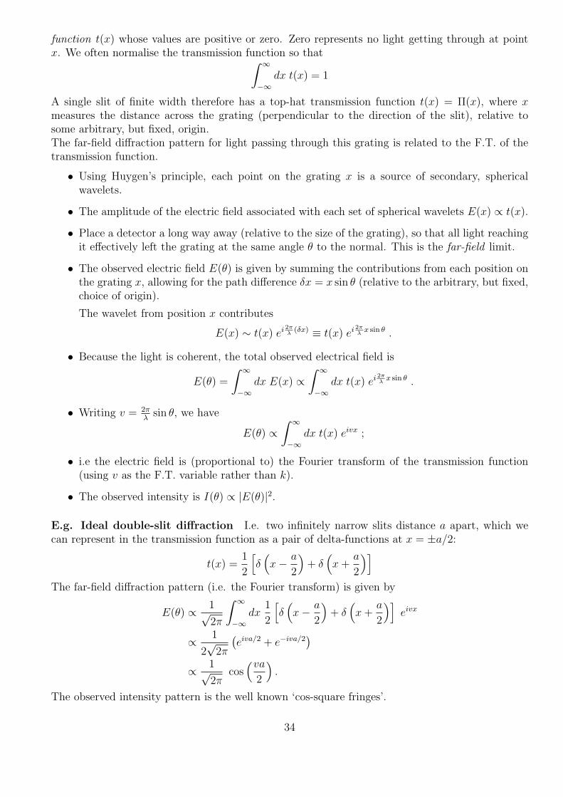
function t(x) whose values are positive or zero. Zero represents no light getting through at pointx. We often normalise the transmission function so that∫ ∞

−∞dx t(x) = 1

A single slit of finite width therefore has a top-hat transmission function t(x) = Π(x), where xmeasures the distance across the grating (perpendicular to the direction of the slit), relative tosome arbitrary, but fixed, origin.The far-field diffraction pattern for light passing through this grating is related to the F.T. of thetransmission function.

• Using Huygen’s principle, each point on the grating x is a source of secondary, sphericalwavelets.

• The amplitude of the electric field associated with each set of spherical wavelets E(x) ∝ t(x).

• Place a detector a long way away (relative to the size of the grating), so that all light reachingit effectively left the grating at the same angle θ to the normal. This is the far-field limit.

• The observed electric field E(θ) is given by summing the contributions from each position onthe grating x, allowing for the path difference δx = x sin θ (relative to the arbitrary, but fixed,choice of origin).

The wavelet from position x contributes

E(x) ∼ t(x) ei2πλ

(δx) ≡ t(x) ei2πλx sin θ .

• Because the light is coherent, the total observed electrical field is

E(θ) =

∫ ∞

−∞dx E(x) ∝

∫ ∞

−∞dx t(x) ei

2πλx sin θ .

• Writing v = 2πλ

sin θ, we have

E(θ) ∝∫ ∞

−∞dx t(x) eivx ;

• i.e the electric field is (proportional to) the Fourier transform of the transmission function(using v as the F.T. variable rather than k).

• The observed intensity is I(θ) ∝ |E(θ)|2.

E.g. Ideal double-slit diffraction I.e. two infinitely narrow slits distance a apart, which wecan represent in the transmission function as a pair of delta-functions at x = ±a/2:

t(x) =1

2

[δ(x− a

2

)+ δ

(x+

a

2

)]The far-field diffraction pattern (i.e. the Fourier transform) is given by

E(θ) ∝ 1√2π

∫ ∞

−∞dx

1

2

[δ(x− a

2

)+ δ

(x+

a

2

)]eivx

∝ 1

2√

2π

(eiva/2 + e−iva/2

)∝ 1√

2πcos(va

2

).

The observed intensity pattern is the well known ‘cos-square fringes’.

34