Physical-chemical properties of complex natural fluids
152
Physical-chemical properties of complex natural fluids Vorgelegt von Diplom-Geochemiker Diplom-Mathematiker Sergey Churakov aus Moskau an der Fakultät VI - Bauingenieurwesen und Angewandte Geowissenschaften - der Technischen Universität Berlin zur Erlangung des akademischen Grades Doktor der Naturwissenschaften - Dr. rer. nat. - genehmigte Dissertation Berichter: Prof. Dr. G. Franz Berichter: Prof. Dr. T. M. Seward Berichter: PD. Dr. M. Gottschalk Tag der wissenschaftlichen Aussprache: 27. August 2001 Berlin 2001 D83
Transcript of Physical-chemical properties of complex natural fluids
Physical-chemical properties of complex natural fluids
Vorgelegt von
Diplom-Geochemiker Diplom-Mathematiker
Sergey Churakov
aus Moskau
an der Fakultät VI
- Bauingenieurwesen und Angewandte Geowissenschaften -
der Technischen Universität Berlin
zur Erlangung des akademischen Grades
Doktor der Naturwissenschaften
- Dr. rer. nat. -
genehmigte Dissertation
Berichter: Prof. Dr. G. Franz
Berichter: Prof. Dr. T. M. Seward
Berichter: PD. Dr. M. Gottschalk
Tag der wissenschaftlichen Aussprache: 27. August 2001
Berlin 2001
D83
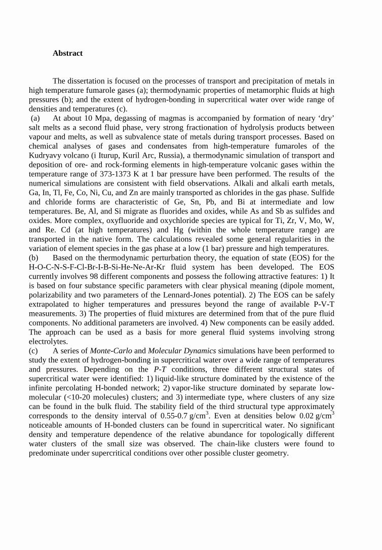
Abstract
The dissertation is focused on the processes of transport and precipitation of metals inhigh temperature fumarole gases (a); thermodynamic properties of metamorphic fluids at highpressures (b); and the extent of hydrogen-bonding in supercritical water over wide range ofdensities and temperatures (c). (a) At about 10 Mpa, degassing of magmas is accompanied by formation of neary ‘dry’salt melts as a second fluid phase, very strong fractionation of hydrolysis products betweenvapour and melts, as well as subvalence state of metals during transport processes. Based onchemical analyses of gases and condensates from high-temperature fumaroles of theKudryavy volcano (i Iturup, Kuril Arc, Russia), a thermodynamic simulation of transport anddeposition of ore- and rock-forming elements in high-temperature volcanic gases within thetemperature range of 373-1373 K at 1 bar pressure have been performed. The results of thenumerical simulations are consistent with field observations. Alkali and alkali earth metals,Ga, In, Tl, Fe, Co, Ni, Cu, and Zn are mainly transported as chlorides in the gas phase. Sulfideand chloride forms are characteristic of Ge, Sn, Pb, and Bi at intermediate and lowtemperatures. Be, Al, and Si migrate as fluorides and oxides, while As and Sb as sulfides andoxides. More complex, oxyfluoride and oxychloride species are typical for Ti, Zr, V, Mo, W,and Re. Cd (at high temperatures) and Hg (within the whole temperature range) aretransported in the native form. The calculations revealed some general regularities in thevariation of element species in the gas phase at a low (1 bar) pressure and high temperatures.(b) Based on the thermodynamic perturbation theory, the equation of state (EOS) for theH-O-C-N-S-F-Cl-Br-I-B-Si-He-Ne-Ar-Kr fluid system has been developed. The EOScurrently involves 98 different components and possess the following attractive features: 1) Itis based on four substance specific parameters with clear physical meaning (dipole moment,polarizability and two parameters of the Lennard-Jones potential). 2) The EOS can be safelyextrapolated to higher temperatures and pressures beyond the range of available P-V-Tmeasurements. 3) The properties of fluid mixtures are determined from that of the pure fluidcomponents. No additional parameters are involved. 4) New components can be easily added.The approach can be used as a basis for more general fluid systems involving strongelectrolytes.(c) A series of Monte-Carlo and Molecular Dynamics simulations have been performed tostudy the extent of hydrogen-bonding in supercritical water over a wide range of temperaturesand pressures. Depending on the P-T conditions, three different structural states ofsupercritical water were identified: 1) liquid-like structure dominated by the existence of theinfinite percolating H-bonded network; 2) vapor-like structure dominated by separate low-molecular (<10-20 molecules) clusters; and 3) intermediate type, where clusters of any sizecan be found in the bulk fluid. The stability field of the third structural type approximatelycorresponds to the density interval of 0.55-0.7 g/cm3. Even at densities below 0.02 g/cm3
noticeable amounts of H-bonded clusters can be found in supercritical water. No significantdensity and temperature dependence of the relative abundance for topologically differentwater clusters of the small size was observed. The chain-like clusters were found topredominate under supercritical conditions over other possible cluster geometry.

Zusammenfassung
Die vorgelegte Dissertation beschäftigt sich mit (a) dem Transport und derKristallisation von verschiedenen chemischen Komponenten in hochtemperierten Fumarolen;(b) den thermodynamischen Eigenschaften von georelevanten Fluiden bei hohen Drucken undTemperaturen; und (c) der Bildung von Wasserstoffbrückenbindungen im überkritischenWasser über einen großen Dichtebereich.
(a) Am Kudryavy Vulkan (Iturup, Kurilen Bogen, Rußland) werdenhochtemperierte Exhalationen beobachtet. Dort steht ein andesitisches Magma bei 10 MPamit zwei weiteren fluiden Phasen im Gleichgewicht. Dabei handelt es sich um eine sehrsalzhaltige kochende flüssige Phase und einen wässrigen Dampf. Zwischen Dampf undFlüssigkeit sind die Hydrolyseprodukte stark fraktioniert. Generell sind diethermodynamischen Eigenschaften aller drei fluiden Phasen stark unterschiedlich, was sichauf die Wertigkeit, die Speziation, die Fraktionierung, die Transporteigenschaften vonElementen und deren Ausfällung in Form von Mineralen auswirkt. Basierend auf chemischenAnalysen der Gase und deren Kondensate wurde ein physikalisch-chemisches Modell desTransportes und der Abscheidung von Erzen beziehungsweise gesteinsbildenderKomponenten angefertigt. Die Ergebnisse der numerischen Simulationen sind mit denFeldbeobachtungen konsistent. Alkali- und Erdalkalimetalle sowie Ga, In, Tl, Fe, Co, Ni, Cuund Zn werden in der Gasphase hauptsächlich in chloridischer Form transportiert. Für Ge, Sn,Pb und Bi sind bei tiefen und mittleren Temperaturen sulfidische und chloridische Komplexecharakteristisch. Be, Al und Si werden in der Form von fluoridischen und oxidischenKomplexen und As und Sb als sulfidische und oxidische Komplexe transportiert. Höherkomplexe Oxysulfid- und Oxychloridverbindungen sind für die Elemente Ti, Zr, V, Mo, Wund Re typisch. Cd wird bei höheren Temperaturen und Hg über den gesamtenTemperaturbereich in elementarer Form transportiert. Mit Hilfe der thermodynamischenBerechnungen konnten einige Gesetzmäßigkeiten des Transport und der Ausfällung vonElementen in hochtemperierten Fumarolen erarbeitet werden.
(b) Unter Verwendung der thermodynamischen „Störungstheorie“ wurde eineZustandsfunktion für Fluide im System H-O-C-N-S-F-Cl-Br-I-B-Si-He-Ne-Ar-Kr entwickelt.Die Zustandsfunktion berücksichtigt 98 verschiedene Spezies und besitzt die folgendenMerkmale: 1. die Zustandsfunktion basiert lediglich auf vier substanzspezifischen Parametermit jeweils eindeutiger physikalischer Bedeutung (Dipolmoment, Polarisierbarkeit und diebeiden Parametern des Lennard-Jones Potentials); 2. die Zustandsfunktion kann zu hohenDrucken und Temperaturen extrapoliert werden; 3. die Eigenschaften der einzelnen Spezies inMischungen kann aus den Eigenschaften des jeweils reinen Fluids abgeleitet werden, undwerden keine zusätzliche Parameter benötigt; 4. weitere Spezies können relativ einfachhinzugefügt werden.
(c) Um die Bedeutung von Wasserstoffbrückenbindungen im überkritischenWasser über einen weiten Temperatur- und Druckbereich zu untersuchen, wurde eine Serievon Monte-Carlo und Molekulardynamischen Simulationen angefertigt. In Abhängig vonDichte und Temperatur konnte im überkritischen Wasser zwischen drei verschiedenen„Stukturzuständen“ unterschieden werden: 1. die „flüssige“ Struktur ist durch eine völligeVernetzung von H2O-Molekülen über Wasserstoffbrückenbindungen charakterisiert; 2. in der„gasförmigen“ Struktur dominieren einzelne Cluster aus wenigen (<10-20) Molekülen; und3. in der „intermediären“ Struktur scheinen Cluster jeder Größe vorzukommen. DasStabilitätsfeld der „intermediären“ Struktur findet man im wesentlichen in einemDichtebereich von 0.55 bis 0.70 g/cm3. Jedoch selbst bei Dichten unter 0.02 g/cm3 konntennoch deutliche Konzentrationen von Clustern festgestellt werden. Am häufigsten scheinenkettenähnliche Cluster vorzukommen. Die Konzentration von H2O-Clustern unterschiedlicherStrukturen scheinen jedoch weder eine Funktion der Dichte noch der Temperatur zu sein.
��������
���������������������� �������������������������������������������
��������� � � ������������������ �������������� �� ��� ��� ����������������
�������� �������������� ������� ���� ������� ���������� �� �������������� ��
��������������������������������������� ��������������������������������
��������������������������������
��� ������!"������ ���������������������������������������������
������� ��������� ���� ����� �������� �� ��� ������������� ��������
���������������������������� ���������������������������������������
����������������� �� �� ����� ���� ������ ���������������� ��������������
�� �� �� �������� �������� ������������ ����������� #� ����� ������� ������
���������������� ��������������� ����������������������$�������� ���%�����
$���������� ���� �������� ���������������� ������������ ������
��������������������������������� ��&����������������������������������
�� �� �$� ���� ��������� �� ����� '��� ��� ��� ��� �� �������� ��������
������������ ��������� �� ������ ����������� �� �������� �������������� (��
&������� �� &���� ��������� �������� �� �����, Ga, In, Tl, Fe, Co, Ni, Cu �� Zn������������ �� �� ��� �� �� �������� ��� �� �� ����� ��������� ����������
#�����������������������������������������Ge, Sn, �����Bi ������ �����������������������������������Si ����������������������������������������������As �Sb- �������������������������Ti, Zr, V, ������� ��������������������� ������
�������������� ��������������������Cd ����� ������� �������������� ��Hg ������� ������������� ����������� ���������������� �� �������� ��������� ��
����� �� �� �������� ������������ ��������� �� ������������� ������
����������� ���������� �� ������� ����������� ��������� �� �� ��� �� �� �
�������������������������������������������
��� #� ����� ������� ���������������� ������ � ��&����� ���
������������������������������)#�����������������������H-O-C-N-S-F-Cl-Br-I-B-Si-He-Ne-Ar-Kr. �� �����&��� ������ )#� ��������� ��� �� ������� ���������� ��������� ������&���� �������� ������������������ ���� )#� ��������� ����� ����� �
���������� ���� ������ �������� ����&��� ������ �� �������� ������ ���������
���������������������� ���������������������������������*�������+������
���� )#� ����� ����� ��������������� ��� ������� ������������ �� ��������� �
��������������&������������������������������������#��������������������
������� �������� ������������ �������� ���� ������� ���������� ���� ,���
���������� ����� ����� �� ��������� ��������� �� ��������� ����������)#� ����
����� � ��� �� ����� ���� �������� ����� ������� ��������� ������� �������
���������������������������
��� !������� ����������� ��������� �� !���$���� ����������
������� �� ����������������� �������� ��� ��� �� ���������������� ���� �
������������������������������ ������������"(��������������������� ������
������������ �������� ������������������� ����� ��� ���������
��������� ��&����������������������������������������� ����������������
����������������������������������������������������������� ���������
��� �������� ��� ����������� �������� �� ����� ���� �������� ��������
��� �������� ������(�������������������������������������������������������
������ �����3��'������������������������������������������������
3��������
���������������� ���� ��� ���� &������ ��������� �������� ����
����������+�������������� ��������������������������� �������� ������������
�������������������������������������������������������������� �� ��
���������������������������������������������������������������
Table of Contents
INTRODUCTION 1
CHAPTER I. Geochemistry and Thermodynamics of High Temperature Volcanic Gases
I.1 Natural fluid phases at high temperatures and low pressures 10
• Abstract 11• Introduction 12• L–V equilibrium 12• Hydrolysis of the salt melt 15• Sublimate minerals formation 17• Native elements 18• Vapour phase species 19• Mass transport by gases 24• Conclusions 25• Acknowledgements 25• References 25
I.2 Evolution of composition of high-temperature fumarolic gases from
Kudrjavy Volcano, Iturup, Kuril Islands: The thermodynamic modelling 28
• Abstract 29• Thermodynamic model 30• Calculation techniques and thermodynamic data 34• Thermodynamic analyses of gas and condensates composition 36• Comparison of the calculated results and the data from natural objects 39• Forms of element transport 43• General regularities of gas transport 55• Conclusions 58• Acknowledgement 58• References 59
CHAPTER II. An Equation of State for Complex Mixtures of Non-Electrolytes
II.1 Perturbation theory based equation of state for polar molecular fluids:
I. Pure fluids 62
• Abstract 63• Introduction 64• Thermodynamic model 68• Limitations of the proposed EOS 71• Derivation methods of the potential parameters for pure fluids 72• Results and discussion 74
• Conclusions 86• Acknowledgement 87• References 87• Appendix II.1 92
II.2 Perturbation theory based equation of state for polar molecular fluids:
II. Fluid mixtures 97
• Abstract 98• Introduction 99• Thermodynamic model 100• Calculated properties in the systems H2O-CO2, H2O-N2 and H2O-CO2-CH4 102• Phase separation at high pressures 108• Conclusions 111• Acknowledgement 111• References 112• Appendix II.2 116
CHAPTER III. Thermodynamics and Structure of Supercritical Water
III.1 Size and topology of molecular clusters in supercritical water:
a molecular dynamics simulation 119
• Abstract 120• Introduction 121• Molecular dynamics simulations 121• Results and discussion 123• Conclusions 129• Acknowledgement 129• References 129
III.2 Size, structure, and abundance of molecular clusters in supercritical water
over wide range of densities: Monte Carlo simulations 131
• Abstract 132• Introduction 133• Method of modeling 133• Results and discussion 134• References 141
LIST OF PUBLICATIONS 143
ACKNOWLEDGEMENT 144
CURRICULUM VITA 145

IINNTTRROODDUUCCTTIIOONN————————————————————————————————————————————————————————————————————————————————————————————————————————————————
1
Fluid phases are involved in various geological and geochemical processes taking
place in the Earth’s crust and upper mantle. For example fluids partly control the rheology of
rocks. They are present on grain boundaries and components like H2O, OH- and H+ can be
incorporated in minerals altering their physical and chemical properties significantly. In
deeper crust, fluids act as solvents dissolving solids and are able to transport and to
concentrate dissolved components. Properties of a fluid phase like its density, compressibility
or viscosity as well as its speciation vary significant with temperature and pressure. Therefore
to explain or to predict a particular geological process the fluid properties must be known in
detail.
In fluids where the concentration of one component is substantially higher than the
concentrations of any other, the main component is called the solvent and the minor
components are the solutes. The nature of the solvent determines the principal properties of
the fluid and governs those of the solutes. In most cases water is the main component of
natural fluids. By studying the properties of even pure water it is therefore possible to predict
the behaviour of natural fluids at various P-T conditions.
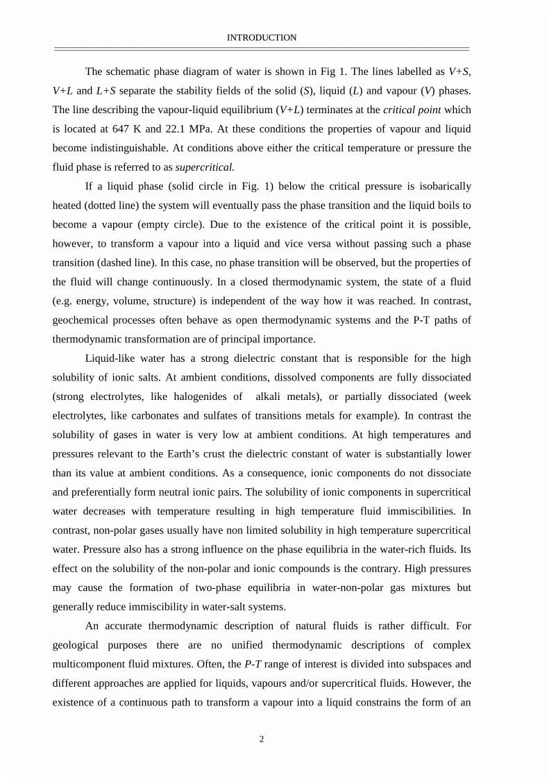
Fig 1. Schematic phase diagram of water.
T
P
647 KTc
Vapor
Liquid (L)
Supercritical Fluid
22.1MPa
Solid (S)
V+L(V)
L+S
V+S
Continous tra
nsitio
n
IINNTTRROODDUUCCTTIIOONN————————————————————————————————————————————————————————————————————————————————————————————————————————————————
2
The schematic phase diagram of water is shown in Fig 1. The lines labelled as V+S,
V+L and L+S separate the stability fields of the solid (S), liquid (L) and vapour (V) phases.
The line describing the vapour-liquid equilibrium (V+L) terminates at the critical point which
is located at 647 K and 22.1 MPa. At these conditions the properties of vapour and liquid
become indistinguishable. At conditions above either the critical temperature or pressure the
fluid phase is referred to as supercritical.
If a liquid phase (solid circle in Fig. 1) below the critical pressure is isobarically
heated (dotted line) the system will eventually pass the phase transition and the liquid boils to
become a vapour (empty circle). Due to the existence of the critical point it is possible,
however, to transform a vapour into a liquid and vice versa without passing such a phase
transition (dashed line). In this case, no phase transition will be observed, but the properties of
the fluid will change continuously. In a closed thermodynamic system, the state of a fluid
(e.g. energy, volume, structure) is independent of the way how it was reached. In contrast,
geochemical processes often behave as open thermodynamic systems and the P-T paths of
thermodynamic transformation are of principal importance.
Liquid-like water has a strong dielectric constant that is responsible for the high
solubility of ionic salts. At ambient conditions, dissolved components are fully dissociated
(strong electrolytes, like halogenides of alkali metals), or partially dissociated (week
electrolytes, like carbonates and sulfates of transitions metals for example). In contrast the
solubility of gases in water is very low at ambient conditions. At high temperatures and
pressures relevant to the Earth’s crust the dielectric constant of water is substantially lower
than its value at ambient conditions. As a consequence, ionic components do not dissociate
and preferentially form neutral ionic pairs. The solubility of ionic components in supercritical
water decreases with temperature resulting in high temperature fluid immiscibilities. In
contrast, non-polar gases usually have non limited solubility in high temperature supercritical
water. Pressure also has a strong influence on the phase equilibria in the water-rich fluids. Its
effect on the solubility of the non-polar and ionic compounds is the contrary. High pressures
may cause the formation of two-phase equilibria in water-non-polar gas mixtures but
generally reduce immiscibility in water-salt systems.
An accurate thermodynamic description of natural fluids is rather difficult. For
geological purposes there are no unified thermodynamic descriptions of complex
multicomponent fluid mixtures. Often, the P-T range of interest is divided into subspaces and
different approaches are applied for liquids, vapours and/or supercritical fluids. However, the
existence of a continuous path to transform a vapour into a liquid constrains the form of an
IINNTTRROODDUUCCTTIIOONN————————————————————————————————————————————————————————————————————————————————————————————————————————————————
3
universal equation of state (EOS) providing the properties of a fluid. The successful EOS
must describe both vapour and liquid simultaneous, as well as the vapour-liquid phase
equilibrium and the critical point. The general approach should take into account all kinds of
interactions between different molecules in the fluid. Some of these types of interaction are
specific to particular chemical components. H2O molecules, for example, are able to form
strong hydrogen bonds, which are to a large degree responsible for its unique chemical and
physical properties.
In this thesis the thermodynamic properties of natural fluids at various temperatures
and pressures are discussed. It contains three chapters that consist of two articles each. These
articles are published together with other scientists. The first chapter covers the geochemistry
and the thermodynamics of high temperature hydrothermal systems associated with recent
magmatic activities. In the second chapter a general equation of state for multicomponent
mixtures of non-electrolytes has been developed. In the third chapter recent investigations
concerning hydrogen bonding in supercritical H2O are compiled. In the following, a general
introduction to these special topics is given.
I. Geochemistry and thermodynamics of high temperature volcanic gases
Gases of complex chemical composition were documented in high temperature
hydrothermal systems associated with active volcanism. It is well established that the main
components of these high temperature fumaroles are H2O, CO2, SO2, H2S, HCl and HF. The
surface temperatures of volcanic gases vary significantly and range from 373K to 1213K. The
gases are produced by boiling of shallow level magmas which are cooled by mixing with cold
meteoric water. This simple model is supported by stable isotope studies (O18/O16, D/H)
which show a strong correlation between the temperature of the gas jets and its fraction of
meteoric water.
Because of low density volcanic gases, it is possible to apply a very simplified but still
accurate thermodynamic description of such systems. Based on these thermodynamic models
one can explain and predict basic peculiarities of the chemical transport and the precipitation
of chemical elements in high temperature hydrothermal systems.
Volcanic gases with the highest temperatures bear direct information of the
composition of the magmas from which they are released, especially in respect to the volatile
and trace element contents leading to ore mineralisation. The contents of ore- and rock-
forming elements in the fumaroles vary between 1 ppb to 100 ppm. This seems to be a very
IINNTTRROODDUUCCTTIIOONN————————————————————————————————————————————————————————————————————————————————————————————————————————————————
4
small number but taking the bulk emission of volcanic gases into account, which is estimated
to be as much as 200 metric tons per day (CONSPEC measurements on Kudriavy volcano,
see the main text for details), the total mass of the ore-forming elements released in few years
of degassing is quite large.
Due to the specific chemistry of the volcanic gas jets their associated mineral
sublimates are in many aspects different from typical hydrothermal mineralisations. The
sublimates form monomineralic clusters of fine grained tiny crystals, mainly chlorides and
sulphides, of ore metals with compositions corresponding to the end members of solid
solution series. Even elements showing extremely small concentration in the gas (about 1-10
ppb) were found to form own minerals. Some of these phases have not been described as
minerals before, because these elements usually enter other phases. For example ReS2 is the
first observation of a natural Re phase. The component ReS2 is usually incorporated in
molybdenite (MoS2). Detailed SEM studies and microprobe analyses of the sublimate samples
indicated the presence of native Al and Si, despite the oxygen fugacities were too high for
these phases to be stable. To explain these observations the dynamic evolution of the
thermodynamic equilibria have to be taken into account.
Field observations on the Kudriavy volcano of the Iturup island (Kuril Island Arc,
Russian far east), have been performed by the members of the Laboratory of Hydrothermal
Fluids of the Institute of Experimental Mineralogy (Chernogolovka, Russia), namely by Dr.
M.A. Korzinsky, Dr. S.I. Tkachenko, and Prof. K.I. Shmulovich between 1988 to 1996. Being
a former member of this group the aim of my work was to develop a thermodynamic model of
the fumarolic activities on the Kudriavy volcano. In the first part of the first chapter the basic
thermodynamic constrains on the low pressure fluid-rock-melts equilibria are discussed. In
the second part the thermodynamic models of the mineral precipitation and the chemical
evolution of the volcanic gases are described in detail.
II. An equation of state for complex mixtures of non-electrolytes
In order to calculate the chemical equilibrium of geological systems the
thermodynamic properties of minerals and fluids are needed. Any equilibrium requires that
the chemical potential of each component is equal in all coexisting phases. If the temperature
and pressure are chosen as the independent variables the chemical potential (µi) of a
component i in a N-component fluid phase can be expressed by the following sum:
IINNTTRROODDUUCCTTIIOONN————————————————————————————————————————————————————————————————————————————————————————————————————————————————
5
µi(T, P, xi ) = µio (T ) + RT ln(Pxi ) + RT ln(ϕ i
o (T ,P)) + RT ln(γ i (T, P, x1,x2, ..., xN )) (1)
where R is the universal gas constant, T the temperature, P the pressure, xi the mole fraction
of component i in the fluid, ϕ io the fugacity of the pure component i and γi the activity
coefficient of the component i in the mixture. The standard chemical potential µio (T ) in eq.
(1) describes the chemical potential of the pure fluid consisting of component i at a pressure
of 0.1 MPa (1 bar) as a function of temperature as it would behave like an ideal gas. The ideal
gas is characterised by molecules which do not interact with others and which do have a
volume of zero. The temperature dependence of µio (T ) arises from the kinetic energy of
molecular motion and from intra-molecular vibrations. It is usually described using the
isobaric heat capacities (cP) which are available for many fluid components. In addition for
simple molecules, the heat capacities can also be calculated using methods provided by
quantum mechanics with an accuracy close to that of the experimental determinations.
As a first approximation, low density fluids can be treated like an ideal gas. The
chemical potential of such a fluid can be calculated using the following simplified expression:
µi(T, P, xi ) = µio (T ) + RT ln(Pxi ) (2)
However, at conditions relevant to the Earth's crust and upper mantle, fluids are quite dense
and therefore their behaviour deviates substantially from that of an ideal gas. These deviations
are due to the intermolecular interaction. In order to account for such effects the fugacity
coefficient ϕ io and the activity coefficient γi are introduced (eq. 1). By definition, γi is unity in
a pure fluid (xi = 1). Therefore, for pure fluids the last term in eq. (1) becomes zero. ϕ io
remains and describes the interaction of molecules of the same kind. In contrast, γi is
attributed to the interaction of different components in fluid mixtures.
Fugacity and activity coefficients can be directly determined using experimental
results of fluid-mineral equilibria or derived from partial molar volumes. In the latter case,
however, the volumes must be known along an isotherm from zero to the pressure of interest.
The fugacity coefficient of a component i in the mixture ϕ i = ϕ ioγ i is given by the following
equation:
IINNTTRROODDUUCCTTIIOONN————————————————————————————————————————————————————————————————————————————————————————————————————————————————
6
RT ln(ϕ i(T ,P, x1, x2 ,..., xN )) =∂V(T, P,x1, x2, ...,xN )
∂ni
−RT
P
dP
0
P
∫ (3)
An integration can be performed using experimentally determined volumes. It is more
convenient, however, to formulate an analytical function with temperature, pressure or
volume and composition as variables and to perform the integration analytically. Such a
function is called an equation of state (EOS).
An EOS can be any function accurately describing the experimental data. However, if
the EOS is only empirical, it might be impossible to extrapolate it to high P-T conditions.
Therefore it is more advantageous to use a theoretically justified EOS, which is based on the
physical nature of fluids. Such EOS can be used in a substantially larger range of
temperatures and pressures.
It was mentioned earlier that real gases deviate from the model of an ideal gas due to
intermolecular interaction. Would the interaction potential be known, fugacity and activity
coefficients could be, at least in principle, calculated using the laws of statistical mechanics.
However, the interactions between polyatomic molecules are very complex and a true
interaction potential would be too complicated for theoretical considerations. Therefore a
model of intermolecular interaction must be simplified in such a way that it is simple enough
for theoretical studies but in the same time still reflects the most important characteristics of
the molecular interaction.
The first successful attempt to formulate an EOS based on intermolecular interaction is
that of van der Waals in 1873. He argued that each molecule in the fluid occupies a finite
volume which cannot be penetrated by other molecules and that the forces acting between
molecules are proportional to the fluid density. These two assumptions lead to the following
EOS:
P =nRT
V − nb−
n2a
V2 (4)
where n is the number of moles and a, b are the van der Waals constants. The intermolecular
interaction is described by these van der Waals constants. The parameter b corresponds
physically to a hypothetical volume of the molecule and the a is a force constant. The van der
Waals model is too simple to provide accurate quantitative results over wide P-T ranges.
However this equation is able to mimic qualitatively the main peculiarities of a fluid phase,
IINNTTRROODDUUCCTTIIOONN————————————————————————————————————————————————————————————————————————————————————————————————————————————————
7
like liquid-vapour equilibria and the supercritical state. Since the discovery of the van der
Waals equation there have been many attempts to improve it by introducing empirical
modifications. These modifications usually include functional temperature and volume
dependencies of the van der Waals constants.
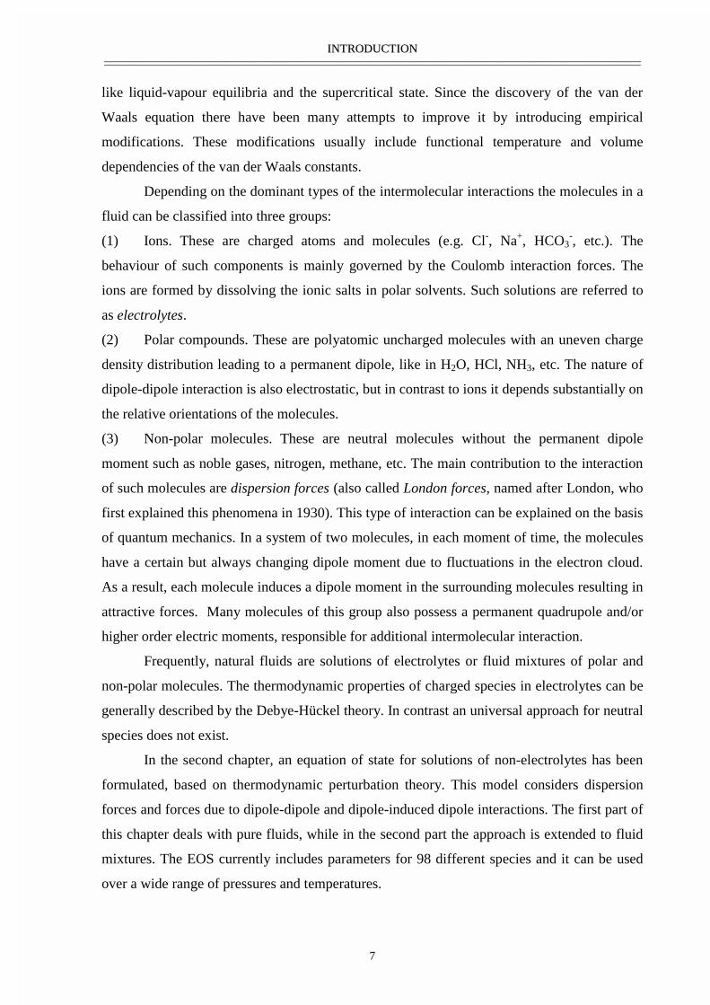
Depending on the dominant types of the intermolecular interactions the molecules in a
fluid can be classified into three groups:
(1) Ions. These are charged atoms and molecules (e.g. Cl-, Na+, HCO3-, etc.). The
behaviour of such components is mainly governed by the Coulomb interaction forces. The
ions are formed by dissolving the ionic salts in polar solvents. Such solutions are referred to
as electrolytes.
(2) Polar compounds. These are polyatomic uncharged molecules with an uneven charge
density distribution leading to a permanent dipole, like in H2O, HCl, NH3, etc. The nature of
dipole-dipole interaction is also electrostatic, but in contrast to ions it depends substantially on
the relative orientations of the molecules.
(3) Non-polar molecules. These are neutral molecules without the permanent dipole
moment such as noble gases, nitrogen, methane, etc. The main contribution to the interaction
of such molecules are dispersion forces (also called London forces, named after London, who
first explained this phenomena in 1930). This type of interaction can be explained on the basis
of quantum mechanics. In a system of two molecules, in each moment of time, the molecules
have a certain but always changing dipole moment due to fluctuations in the electron cloud.
As a result, each molecule induces a dipole moment in the surrounding molecules resulting in
attractive forces. Many molecules of this group also possess a permanent quadrupole and/or
higher order electric moments, responsible for additional intermolecular interaction.
Frequently, natural fluids are solutions of electrolytes or fluid mixtures of polar and
non-polar molecules. The thermodynamic properties of charged species in electrolytes can be
generally described by the Debye-Hückel theory. In contrast an universal approach for neutral
species does not exist.
In the second chapter, an equation of state for solutions of non-electrolytes has been
formulated, based on thermodynamic perturbation theory. This model considers dispersion
forces and forces due to dipole-dipole and dipole-induced dipole interactions. The first part of
this chapter deals with pure fluids, while in the second part the approach is extended to fluid
mixtures. The EOS currently includes parameters for 98 different species and it can be used
over a wide range of pressures and temperatures.
IINNTTRROODDUUCCTTIIOONN————————————————————————————————————————————————————————————————————————————————————————————————————————————————
8
III. Thermodynamics and structure of supercritical water
To develop an accurate thermodynamic model for a fluid it is necessary to understand
its structure. In contrast to solids, constituents of fluids are mobile and do not occupy even on
average definite places. However, not every relative orientation of molecules is favourable, so
that molecular motion is not random, but substantially correlated. This correlation can be
characterised by different statistical quantities like the velocity autocorrelation function, the
radial distribution function, the structure factor and some other parameters used in solid state
physics and as well crystallography.
Both experimental and theoretical methods can be applied to analyse fluid structures.
The structure factor can be obtained from X-ray and neutron diffraction studies. Parameters
of the intra-molecular and intermolecular interactions as well as the structure of molecular
clusters can be derived from spectroscopic measurements. These measurements are rather
complicated especially at high temperatures and pressures. In many cases, particularly in
spectroscopy, the results are equivocal allowing various interpretations. Theoretical computer
models can be used as an alternative. Certainly, molecular simulations can not fully substitute
experimental measurements, because they need some results from experimental studies as
input. Even the most powerful ab initio calculations imply a variety of approximations which
lead to uncertainties. Nevertheless, such simulations provide a fast and reliable look inside
fluid properties, which are sometimes much more detailed than one could expect from
conventional experimental methods.
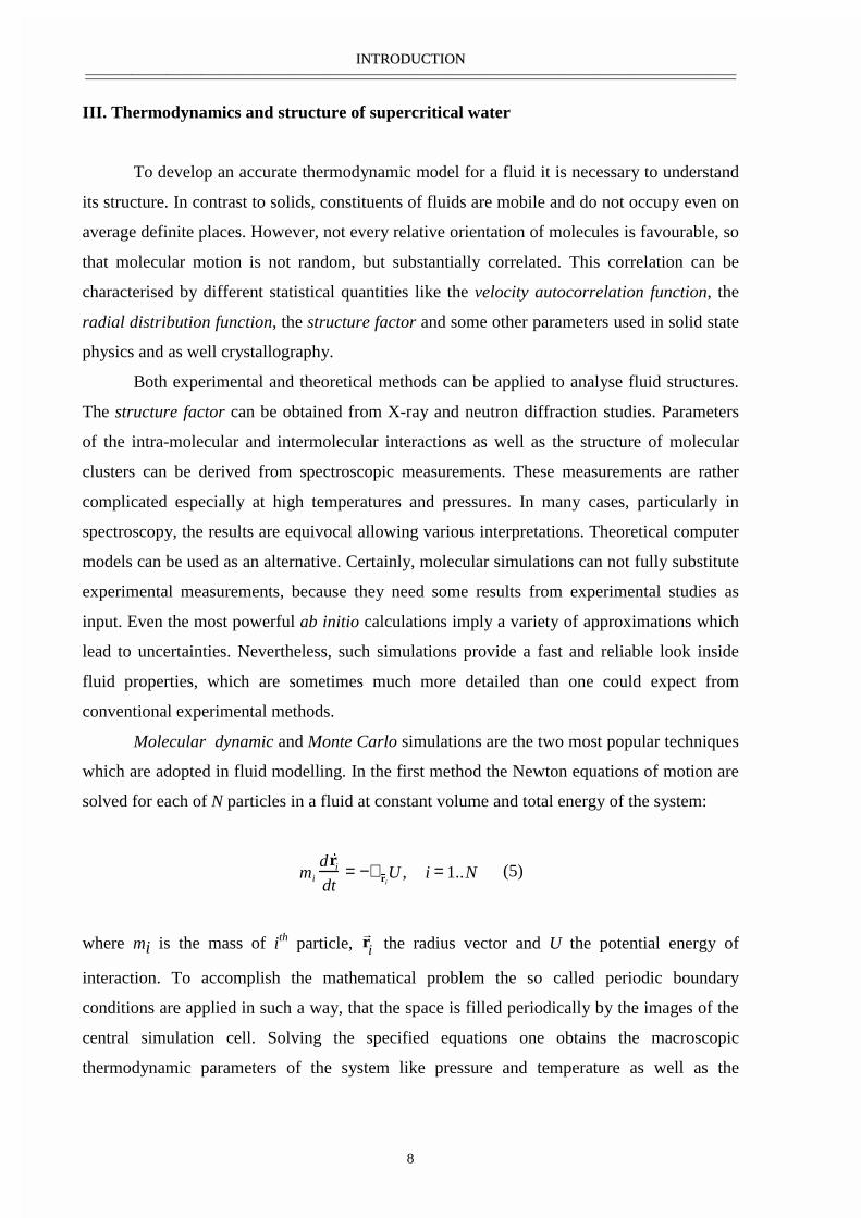
Molecular dynamic and Monte Carlo simulations are the two most popular techniques
which are adopted in fluid modelling. In the first method the Newton equations of motion are
solved for each of N particles in a fluid at constant volume and total energy of the system:
mi
d&
r idt
= −∇ &
r iU , i = 1..N (5)
where mi is the mass of ith particle, ��
��
r i the radius vector and U the potential energy of
interaction. To accomplish the mathematical problem the so called periodic boundary
conditions are applied in such a way, that the space is filled periodically by the images of the
central simulation cell. Solving the specified equations one obtains the macroscopic
thermodynamic parameters of the system like pressure and temperature as well as the
IINNTTRROODDUUCCTTIIOONN————————————————————————————————————————————————————————————————————————————————————————————————————————————————
9
trajectories of molecular motion, which can be analysed to get the statistical quantities
characterising the fluid structure.
In Monte Carlo simulations a Markov chain of molecular configurations is generated
using random numbers which satisfies a particular statistical distribution. The Markov chain
of states is a sequence of trials that satisfies the following two conditions: (a) the outcome of
the trial belongs to a finite set of outcomes; (b) the outcome of each trial depends only on the
outcome of the trial which immediately precedes it. For example at constant volume and
temperature, starting from an arbitrary molecular configuration with the potential energy Uold,
the new state is generated by translating and rotating the particles of a fluid at random. If the
energy of the new configuration Unew is smaller then the Uold, the new configuration is
immediately accepted. If Unew is larger than Uold then the new configuration will be accepted
only with a probability which is proportional to exp((Uold - Unew)/kT), where k is the
Boltzmann constant and T the temperature. Otherwise, the new configuration is rejected and
the old configuration is used again. Then the procedure is repeated.
Both molecular dynamics and Monte Carlo methods use various approximations for
the potential energy of intermolecular interactions. The choice of intermolecular potentials is
of principle importance, because it governs the accuracy of the calculations. Thus each
potential model is a compromise between accuracy and simplicity.
In most typical geological fluids, H2O is the main component. Therefore to formulate
a model for multicomponent mixtures, it is necessary to understand the behaviour of pure
water. It is well established that the structure of liquid water at ambient conditions as well as
the structure of ice is attributed to strong hydrogen bonding. The hydrogen bond is a
particular type of intermolecular interaction which is observed between hydrogen and an
electronegative atom of a different molecule. The physical nature of this effect consists of the
fact, that the electron density around a hydrogen atom can be deformed. Therefore, such a
hydrogen atom is partly charged and can constructively interact with other molecules.
However, up to recently, the important role of hydrogen bonding at high temperatures have
been mostly neglected. Molecular dynamic and Monte Carlo simulations have been applied to
analyze the extend of hydrogen bonding and the structure of water in a temperature interval
between 573 and 773K and densities of up to about 1 g/cm3. The results are summarized in
two articles constituting the third chapter of the dissertation.

Natural Fluid Phases at High Temperatures and low Pressures
CCHHAAPPTTEERR 11.. GGeeoocchheemmiissttrryy aanndd TThheerrmmooddyynnaammiiccss ooff hhiigghh TTeemmppeerraattuurree VVoollccaanniicc GGaasseess————————————————————————————————————————————————————————————————————————————————————————————————————————————————
11
Abstract
Gas phases at low pressures and high magmatic temperatures have certain peculiar
properties. The fluid is mainly water vapour, which is usually observed during discharging of
crystal magmatic melts. At pressures about 100 bar these peculiar properties include:
formation of near ‘dry’ salt melts as second fluid phase, very strong fractionation of
hydrolysis products between vapour and melts, subvalence state of metals during transport
processes, and high sensitivity of the gas to conditions of sublimate precipitation. Phase
diagram analysis as well as results of field and laboratory experiments are presented in this
article. The processes could be a model for industrial technologies to clean wastes from toxic,
rare and heavy metals. Transport forms of some elements in volcanic gases are very similar to
the species which were formed first in the protosolar nebula.
Keywords: gas phase; gas condensates; brines; solution transport; native elements
CCHHAAPPTTEERR 11.. GGeeoocchheemmiissttrryy aanndd TThheerrmmooddyynnaammiiccss ooff hhiigghh TTeemmppeerraattuurree VVoollccaanniicc GGaasseess————————————————————————————————————————————————————————————————————————————————————————————————————————————————
12
1. Introduction
Gas pollution is a serious problem in modern environments and will only increase in
the next century. The principles of geochemical engineering, i.e. the organisation of industrial
processes to protect our environment by the same way as natural processes (Schuiling, 1990),
could be applied to clean industrial gases from heavy, toxic and rare elements, but we must
know how these natural processes are regulated. The best way to investigate these processes is
by studying volcanic gases which contain practically all elements, and these compositions can
be used as a model for industrial gas pollution. This article is a short review of new field and
laboratory results which were obtained from the Kudriavy volcano (andesitic Kuril Island
Arc, Russian Far East) from 1988 to 1996, where very hot fumaroles of 170–940°C exist in a
stationary regime dating from the last explosion in 1873. The main analytical and
mineralogical data for the fumarole gases and sublimates are published by Korzhinsky et al.
(1994, 1995, 1996) and Taran et al. (1995); some of the data are still in preparation. These
high-temperature fumaroles have relatively constant compositions of 94–95 mol% of H2O,
about 2 mol% each of various C and S species and 0.5 mol% HCl. A maximal H2
concentration of 1.2 mol% was found in the hottest fumarole 940°C. Oxygen fugacities were
found to fall within the ‘inner’ gas buffer, which mainly depend on the temperature of
equilibrium between sulphuric species (SO2, H2S, S2), H2 and H2O. This equilibrium is very
near to the Ni–NiO buffer, which can be used for calculations. Calculation of oxygen
fugacities using the ratios SO2/H2S and CO2/CO are in good agreement with direct
measurements of fO2 by solid state electrolyte cells (Rosen et al., 1993)
2. L–V equilibrium
Degassing of a magmatic melt at low pressure can take place if the magma chamber is
in connection with the surface via gas conduits, and the pressure on the uppermost part of the
chamber is not too large. Gas viscosity and, consequently, gasodynamic resistance are small
and for conduits with a characteristic size of 1–10 cm, the Darcy equation indicates only a
pressure of 5–20 bar on the magma surface at intermediate crust chambers, 2–3 km under the
volcanic summit. Stable isotope data for D/H and 18O /16O ratios support these estimations, as
the boiling of meteoric water and beginning of mixing meteoric and magmatic water take
place at 170–180°C, which corresponds to a pressure of 8–10 bar.
CCHHAAPPTTEERR 11.. GGeeoocchheemmiissttrryy aanndd TThheerrmmooddyynnaammiiccss ooff hhiigghh TTeemmppeerraattuurree VVoollccaanniicc GGaasseess————————————————————————————————————————————————————————————————————————————————————————————————————————————————
13
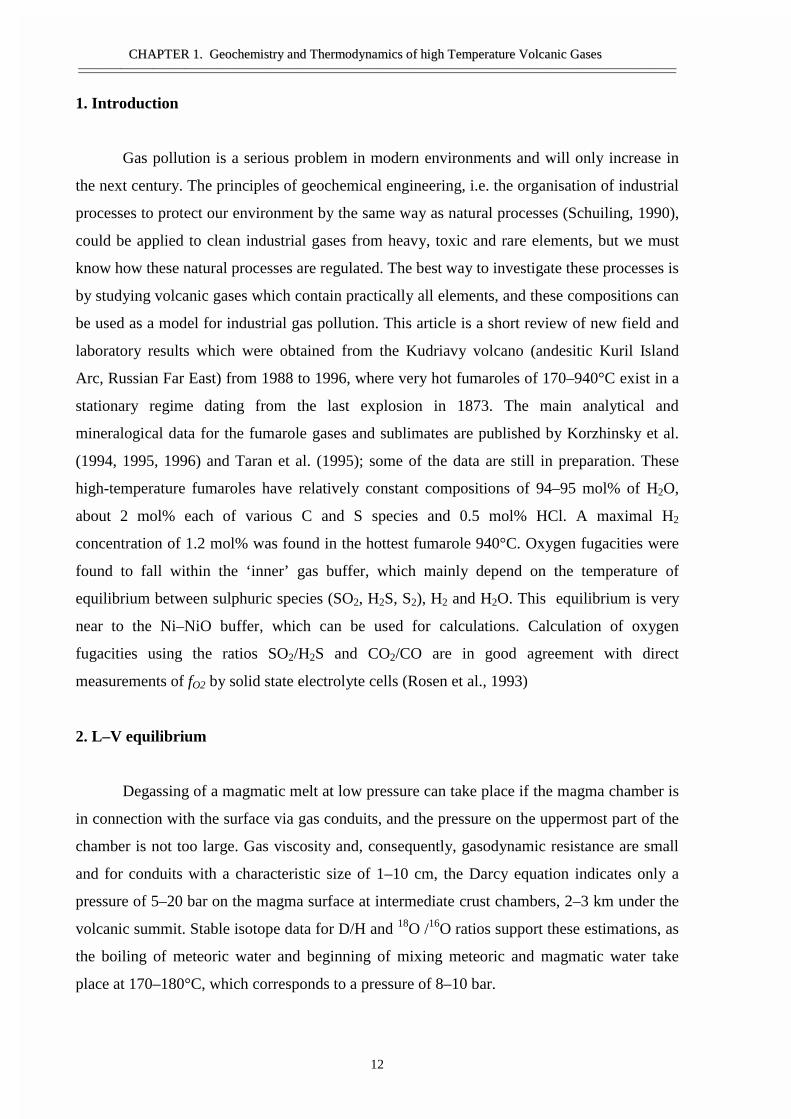
Fig. 1. Ratio of fluid components in the fluid and magmatic melt at 0.1 and 0.5 kbar and a simplifiedphase diagram for the H2O–NaCl system. If at low pressure the magmatic melt is in equilibrium withthe fluids, then the composition of the brine is going along the saturation curve (Halite+L) and in factthree phases are stable (+V). Above 800°C the salt melt is practically dry.
At such low pressures and with magmatic temperatures of 800–1000°C, the phase
state and composition of the fluid have some specific properties. Two isobaric diagrams 100
and 500 bar are presented in Fig. 1. Both diagrams are a superposition of the melting
diagrams showing the ratio H2O/(CO2 or NaCl) in the fluid and coexisting haplogranitic
melts, and liquid–vapour–solid diagrams for the system H2O–NaCl (Bodnar et al., 1985;
Bischoff and Pitzer, 1989). The melting diagrams for 0.5 and 0.1 kbar were obtained via the
linear interpolation of data from Keppler (1989) for wet and dry melting haplogranite
composition in a T–log P space. On the diagram we can see that at 0.5 kbar, magma
degassing produces two fluid phases if the magma contains enough Cl, i.e. at a normal
H2O/Cl ratio near 10. During cooling of these fluid phases their compositions evolves along
lines ‘L’ and ‘V’ up to the critical point (C.P.). At a pressure of 100 bar the vapour phase is
practically pure water (at 500°C the NaCl concentration is below 0.02 wt.%) and therefore
must be drawn along the ordinate axis. The liquid phase is undersaturated or saturated with
respect to solid salt (halite). The diagram was drawn for pure NaCl; in fact, for a magmatic
0.1 kbar, L
Satur
ated
,
Halite
+ L
V L0.5 kbar
Melt
Fluid, 0.5 kbar0.1 kbar
300
400
500
600
700
800
900
1000
0 20 40 60 80 100
Tem
pera
ture
(˚C
)
C.P.
wt. %, NaCl (CO2)
CCHHAAPPTTEERR 11.. GGeeoocchheemmiissttrryy aanndd TThheerrmmooddyynnaammiiccss ooff hhiigghh TTeemmppeerraattuurree VVoollccaanniicc GGaasseess————————————————————————————————————————————————————————————————————————————————————————————————————————————————
14
melt that separates out a salt mix, the temperatures of saturation for the solid salts must be
lower. Fluid phase equilibrium shows that at low pressures and high temperatures the normal
process of magma degassing must produce two fluids — vapour and dry salt melt.
Field observations support this conclusion. The original melt from the Kudriavy
volcano has a Cl content of 0.3 wt.% (melt inclusions, Tzareva, pers. commun., 1994). This is
a quite normal concentration for andesitic melts. Water content is not known, but andesitic
melts typically contain near 2–3 wt.% of H2O. The weight ratio of H2O/Cl in the melt is about
10. In gas samples collected from the Kudriavy volcano the mean ratio of H2O/Cl is 100–200,
and therefore more than 90% of the chlorine is refined within the magma chamber as a salt
melt. The viscosity of salt melts is approximately 4–6 orders of magnitude lower than that of
andesitic melts and densities are approximately 0.5–0.6 of the andesitic melts. With so large
differences in density and viscosity it would seem that salt melts would naturally collect on
the surface of degassing magma as a separate phase. Semi-quantitative calculations for the
Kudriavy volcano give a volume for the salt melt of approximately 3·106 m3 after 114 years of
passive stationary degassing.
It must be remarked that during the degassing process, the magma volume will
decrease with the value of partial volume of the discharged gases mainly water from the melt
and that this effect will result in additional space for the salt melt. After 114 years of
degassing for the assumed primitive geometry of a spherical magmatic chamber with a
diameter of 2 km, an ‘empty’ spherical segment with a volume of 2·107 m3 will have been
produced. The salt layer takes the form of a disk with a diameter of 1.3 km and a thickness of
about 2 m. Of course, in the actual scenario we expect the collapse of overlying rocks. Also
the shape of the salt melt will be quite irregular and locally much thicker. These conclusions
may be incorrect for basaltic melts, since these melts usually contain 0.5 wt.% water and, at
1200–1300°C, the rate of evaporation (vapour pressure) of the salt can be too large to keep a
salt melt on the top of the magma chamber. Formation of salt melts leads to ternary coexisting
mobile phases: gas + salt-melt + silicate-melt, which are near equilibrium.
CCHHAAPPTTEERR 11.. GGeeoocchheemmiissttrryy aanndd TThheerrmmooddyynnaammiiccss ooff hhiigghh TTeemmppeerraattuurree VVoollccaanniicc GGaasseess————————————————————————————————————————————————————————————————————————————————————————————————————————————————
15
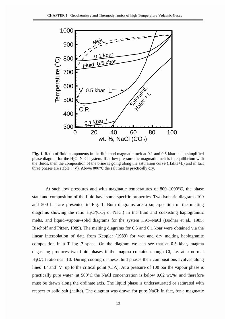
Fig. 2. Acid-base fractionation between the liquid and vapour phases in the systems H2O–NaCl(Vakulenko et al., 1989) and H2O–CaCl2 calculated from the data of Bischoff et al. (1996). The pointsfor the CaCl2 system are our measurements of pH quenched vapour solutions from sampling in thesystem H2O–CaCl2 (Tkachenko and Shmulovich, 1992).
3. Hydrolysis of the salt melt
At a liquid–vapour equilibrium, if the vapour phase is practically pure water, we
should observe the effect of the fractionation of the hydrolysis products between coexisting
phases. One such simple reaction is: H2O + NaCl = HCl + NaOH. At high pressure (above
500 bar) this reaction has a strong shift to the left, but at magmatic temperatures and low
pressures (below 100 bar) the process of fractionation begins to play an important role. The
fugacities (or vapour pressures) of HCl and NaOH differ significantly, and HCl will go into
the vapour phase and NaOH into the liquid phase. This is the principal reason for the acidity
of volcanic gases. Experiments and field observations are in good agreement on this point.
Fig. 2 presents an extrapolation of data from Vakulenko et al. (1989) by the equation for the
pH of the quenched vapour phase:
pH = 9.891 - 9.943 · T(°C) · 10-3
0 2 4 6 8 10 1412300
400
500
600
700
800
900
1000
NaCl LV
CaC
l2pH, quenched solution
Tem
pera
ture
(˚C
)
CCHHAAPPTTEERR 11.. GGeeoocchheemmiissttrryy aanndd TThheerrmmooddyynnaammiiccss ooff hhiigghh TTeemmppeerraattuurree VVoollccaanniicc GGaasseess————————————————————————————————————————————————————————————————————————————————————————————————————————————————
16
Extrapolation from 350–650°C to 1000°C gives for the hottest fumarole on the Kudriavy
volcano 940°C a pH of 0.544, which corresponds to 0.51 mol% HCl. The measured
concentration of HCl in the condensed fumarole gas phase at the same temperature is 0.46
mol%. Of course, the salt melt is not pure NaCl and the concentrations of HCl from other hot
fumaroles (500–900°C) lie between the hydrolysis curves for NaCl and CaCl2 (Bischoff et al.,
1996). This strong hydrolysis reaction and the fractionation products between coexisting fluid
phases lead to the formation of contrasting acidity between hydrothermal solutions, i.e. acid
springs associated with volcanic areas and albitization of granitic rocks during postmagmatic
processes.
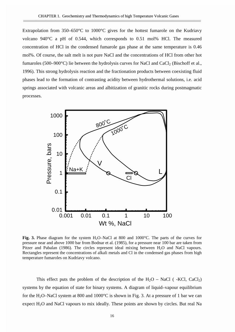
Fig. 3. Phase diagram for the system H2O–NaCl at 800 and 1000°C. The parts of the curves forpressure near and above 1000 bar from Bodnar et al. (1985), for a pressure near 100 bar are taken fromPitzer and Pabalan (1986). The circles represent ideal mixing between H2O and NaCl vapours.Rectangles represent the concentrations of alkali metals and Cl in the condensed gas phases from hightemperature fumaroles on Kudriavy volcano.
This effect puts the problem of the description of the H2O – NaCl ( -KCl, CaCl2)
systems by the equation of state for binary systems. A diagram of liquid–vapour equilibrium
for the H2O–NaCl system at 800 and 1000°C is shown in Fig. 3. At a pressure of 1 bar we can
expect H2O and NaCl vapours to mix ideally. These points are shown by circles. But real Na
0.001 0.01 0.1 1 10 100
1000
100
10
1
0.1
0.01
Na+KV
LCl
800˚C
1000˚C
Wt %, NaCl
Pre
ssur
e, b
ars
CCHHAAPPTTEERR 11.. GGeeoocchheemmiissttrryy aanndd TThheerrmmooddyynnaammiiccss ooff hhiigghh TTeemmppeerraattuurree VVoollccaanniicc GGaasseess————————————————————————————————————————————————————————————————————————————————————————————————————————————————
17
and K concentrations in condensed volcanic gases are 2–2.5 orders of magnitude lower than
shown in the diagram for the binary system. Evolution of fluid phase compositions as a
function of decreasing pressure follows the solid line from a pressure of above 1000 bar down
to 200 bar. But below 100 bar the vapour composition is essentially nonbinary. Cation
concentrations go along the dashed line, but Cl- behaves as if it were still in the binary system.
The fluid phase ‘L’, the magmatic melt and the vapour are not so far from equilibrium at
temperatures of 700°C and higher. It is obvious why condensed volcanic gases have a low
pH, e.g. similar condensed gases from the Kudriavy volcano have a pH < 0. It is the same
effect as was found for the system H2O–CaCl2 (Bischoff et al., 1996) and was predicted by
Khitarov (1954) nearly half a century ago.
4. Sublimate minerals formation
Long-time experiments for sublimate formation were done on the Kudriavy volcano.
Maximal duration of the runs was nearly 1 month. The sublimates precipitated inside quartz
glass tubes, 2/3 of which was exposed above the surface and 1/3 was buried below. In the
tubes were found: halogenides (simple as NaCl and KCl), and more complicated (KPb2Cl5,
marshite, CuI, and some fluorine minerals), oxides (SiO2, Al2O3, KReO4), sulphides, silicates
and sulphates. Detailed description of sublimate mineralogy is beyond the scope of this
article, but some remarks need to be made, principally from field observations. The discovery
of the ore deposit of Re (Korzhinsky et al., 1994) demonstrates that sublimate minerals can
precipitate from the gas phase even at very low metal concentrations. For example, the
concentration of Re in the condensed vapour phase was never above 10 ppb, but ReS2 covers
the surface of each 2 rock sample in the zone of these deposits where fumarole temperatures
were between 500 and 650°C. In the tubes particles of Au and Pt were found, despite the fact
that bulk Au and Pt concentrations were below the detection limit of the ICP analysis - 1 ppb.
The main rules for a process of sublimate precipitation were summarised by Schafer (1964,
1981), derived from experimental investigations of chemical reactions with transport through
a gas phase. For sublimate minerals many parameters can play an important role, e.g.
individual concentrations of both gas species and metallic components, temperature, oxidising
state, nucleation of the phase, gas velocity, properties of the precipitation surface, etc.
Our field experiments and laboratory investigations of samples have demonstrated the
following.
CCHHAAPPTTEERR 11.. GGeeoocchheemmiissttrryy aanndd TThheerrmmooddyynnaammiiccss ooff hhiigghh TTeemmppeerraattuurree VVoollccaanniicc GGaasseess————————————————————————————————————————————————————————————————————————————————————————————————————————————————
18
(1) Sublimate minerals usually form relatively large clusters, with many crystals
connected together as a monomineral group. Not only the more abundant minerals form these
types of clusters such as SiO2, NaCl and KCl, but also aegirin, molybdenite, wurzite,
KPb2Cl5, K3CdCl5, as well as a series of unknown phases form clusters. One of such
unknown phases contains K, Mo and S (analysed by SEM-EDAX). The crystals have a
cylindrical shape with near 1 µm diameter and 20–40 µm length, with hollow centres.
(2) While these sublimate phases readily precipitate in quartz glass tubes, graphite
tubes remained clean even if they were exposed some days. Mullite ceramic tubes were
usually destroyed by rain and wind, while metallic tubes corroded after short runs.
(3) Natural sublimates are mainly the products of reactions between primary phases
precipitated from volcanic gases and acid rain. The acid rain was formed by mixing of the
volcanic gas components HCl, SO2 and HF with rain water.
Temperature zonality of the sublimate minerals was found in a number of tubes, but
air cooling of the open part of the tubes at the very unstable weather on the Kuril Islands leads
to variable temperature gradients inside the tubes and some mineral zones thus overlap. The
same results (mixture of temperature zones) were produced by the filling of the tubes by
sublimates, thereby decreasing heat flow. One of the tubes was fully blocked by sublimates,
with mainly native sulphur at the cold end. More detailed investigations, in which the
temperature is controlled, are needed to distinguish the separate precipitation of heavy, toxic
and rare metals from the volcanic gases as a function of temperature.
Calculations of sublimate precipitation from real gas compositions usually correspond
to the succession of minerals found inside the tubes within a relatively large temperature
interval. This large interval is partly caused by air cooling.
5. Native elements
Some native elements are quite common in rocks, e.g. noble metals, sulphur, iron,
carbon, etc. In the Russian literature since 1981, many articles were published about quite
unusual native metals (Al, Si, Mg, Bi, Pb) in kimberlites, trapps, granites and hydrothermal
ore deposits (Novgorodova, 1983). Calculations concerning the stability fields of these metals
lead to unrealistic fluid compositions (Novgorodova, 1996), which were practically pure
methane or hydrogen. However, the many occurrences of these native metals indicate that the
processes forming these minerals are much more common than can be explained from such
exotic fluids.
CCHHAAPPTTEERR 11.. GGeeoocchheemmiissttrryy aanndd TThheerrmmooddyynnaammiiccss ooff hhiigghh TTeemmppeerraattuurree VVoollccaanniicc GGaasseess————————————————————————————————————————————————————————————————————————————————————————————————————————————————
19
We observed the formation of native Al, Si and Al–Si alloys directly inside the quartz
glass tubes (Korzhinsky et al., 1995, 1996), where any contamination was excluded. The gas
composition and oxygen fugacities of the gas jets were also measured (Rosen et al., 1993).
Real conditions were found to be far from the equilibrium state. For example, for native Al to
be stable the oxygen fugacities should be 31 orders of magnitude (!) below the measured
value. The stability field for native Si is at an oxygen fugacity 23 orders of magnitude below
the Ni–NiO buffer, which corresponds to the measured conditions in the gases. High H2
contents in volcanic gases or hydrothermal fluids, which could stabilise such metals, were not
observed. Therefore we need to find another explanation for the formation of these low
oxidising metals. Perhaps, some of them indicate which gas species were present in the fluid
at magmatic temperatures and relatively low pressures.
6. Vapour phase species
Calculations for metal transport by volcanic gases were done for the Momotombo
(Quisefit et al., 1989), Augustin (Symonds et al., 1992) and St. Helens volcanoes (Symonds
and Reed, 1993). From the database and software of Symonds and Reed (1993) the main
species in those gases for rock-forming and ore elements include chlorides (MnCl2, CoCl2,
CuCl, AgCl, KCl, NaCl, RbCl, CaCl2, CsCl), (hydr-)oxides (Fe(OH)2, H2WO4, H2MoO4),
elements (Zn, Cd, Hg), sulphides (PbS, AsS, SbS, AuS), and fluorides (SiF4, AlOF2). These
calculations agree with minerals of incrustations derived from fumarole jets except for Pb:
this forms PbS galena in the incrustations, which is not one of the sulphide species in the
gases.
Our calculations were done using the database IVTANTERMO (Glushko, 1978) and
the gas composition of the hottest fumarole jet 940°C as the most representative magmatic
gas. Calculations of gas species included 45 elements: H, O, Cl, F, S, C, Br, Li, Na, K, Rb,
Cs, Be, Mg, Ca, Sr, Ba, Al, Ga, In, Tl, Si, Ge, Sn, Pb, As, Sb, Bi, Cu, Zn, Cd, Hg, Ti, Zr, V,
Nb, Ta, Cr, Mo, W, Mn, Re, Fe, Co, and Ni. The existing database does not cover all possible
species, especially for the rare elements. Therefore, the results are given for the more common
mineral species, like sulphides, chlorides, etc.
6.1. Elements Li, Na, K, Rb, Cs
At temperatures above 600°C the most abundant transport form of these elements is in
the form of metal–Cl. Concentrations of these chlorides depend on the source of the gas phase
CCHHAAPPTTEERR 11.. GGeeoocchheemmiissttrryy aanndd TThheerrmmooddyynnaammiiccss ooff hhiigghh TTeemmppeerraattuurree VVoollccaanniicc GGaasseess————————————————————————————————————————————————————————————————————————————————————————————————————————————————
20
and concentrations of the chlorides as defined by precipitation of LiCl, NaCl, KCl, etc. In
high-temperature experiments (>700°C) NaCl and KCl are the most abundant mineral
sublimates and they form the inner rim in the sampling tubes.
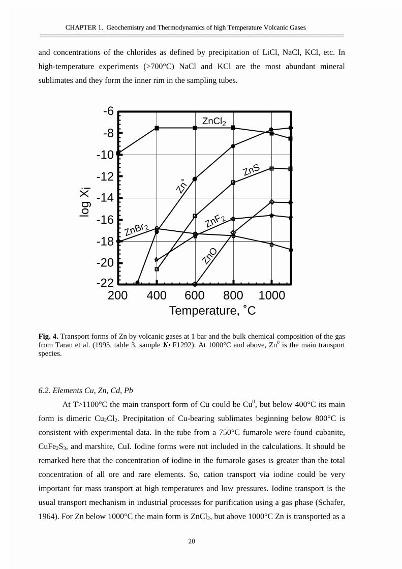
Fig. 4. Transport forms of Zn by volcanic gases at 1 bar and the bulk chemical composition of the gasfrom Taran et al. (1995, table 3, sample � F1292). At 1000°C and above, Zn0 is the main transportspecies.
6.2. Elements Cu, Zn, Cd, Pb
At T>1100°C the main transport form of Cu could be Cu0, but below 400°C its main
form is dimeric Cu2Cl2. Precipitation of Cu-bearing sublimates beginning below 800°C is
consistent with experimental data. In the tube from a 750°C fumarole were found cubanite,
CuFe2S3, and marshite, CuI. Iodine forms were not included in the calculations. It should be
remarked here that the concentration of iodine in the fumarole gases is greater than the total
concentration of all ore and rare elements. So, cation transport via iodine could be very
important for mass transport at high temperatures and low pressures. Iodine transport is the
usual transport mechanism in industrial processes for purification using a gas phase (Schafer,
1964). For Zn below 1000°C the main form is ZnCl2, but above 1000°C Zn is transported as a
ZnCl2
Zn˚
ZnS
ZnBr2 ZnF2
ZnO
Temperature, ˚C200 400 600 800 1000
log
Xi
-22
-20
-18
-16
-14
-12
-10
-8
-6
CCHHAAPPTTEERR 11.. GGeeoocchheemmiissttrryy aanndd TThheerrmmooddyynnaammiiccss ooff hhiigghh TTeemmppeerraattuurree VVoollccaanniicc GGaasseess————————————————————————————————————————————————————————————————————————————————————————————————————————————————
21
metal, Zn0. This is illustrated in Fig. 4. Wurzite was a common sublimate mineral in our
tubes, but the ZnS concentrations were smaller than ZnCl2 and Zn0 at all temperatures. The
same behaviour was found for Cd, but here the change of transport form, from native metal to
chloride, is at 600°C. According to calculations and observations, below this temperature Cd
is precipitated as grinokite and K3CdCl5. For Pb above 600°C the dominant form is PbS,
below 600°C the dominant form is PbCl2.
6.3. Elements As, Sb, Bi, Hg
The transport forms of As change with temperature. Up to 600°C As4S4 and As4O6
dominate in the gas phase. Above 600°C the main form is AsS, and only above 1100°C does
the oxide, AsO dominate. The main transport forms of Sb change from SbF3 below 300°C, to
Sb4O6 up to 600°C and SbS above 600°C. At relatively low temperatures Bi and Hg are
transported as chlorides. BiCl dominates below 600°C. However, HgCl2 is an artefact, since
this form dominates below 100°C, where water will condense and a gas phase does not exist.
At high temperatures Bi and Hg are transported as elements.
6.4. W and Mo
The concentrations of these metals in the fumarole gases are 3–60 ppb for W and 2–
300 ppb for Mo. The main transport forms are WCl2O2 at all temperatures, and MoCl2O2
below 700°C and H2MoO4 above. However the database for these elements is very limited.
6.5. Re, In and Tl
These elements are interesting because Re and In minerals were discovered in the
natural sublimates as well as in ore deposits of ReS2. The database is also limited for Re. For
all temperatures ReClO3 was indicated to be the main form. But ore deposits contain Re
sulphide and in the sampling tubes we only found KReO4. Species of In are more simple. The
dominant forms are InCl3 below 350°C, InCl2 between 350 and 600°C and InCl at higher
temperatures. In some condensed gas samples, very high concentrations of Tl were found.
Usually concentrations are between 60 and 200 ppb, but in one fumarole at a temperature of
605°C we found concentrations of Tl near 4 ppm. At all gas temperatures the main transport
form for Tl is TlCl.
CCHHAAPPTTEERR 11.. GGeeoocchheemmiissttrryy aanndd TThheerrmmooddyynnaammiiccss ooff hhiigghh TTeemmppeerraattuurree VVoollccaanniicc GGaasseess————————————————————————————————————————————————————————————————————————————————————————————————————————————————
22
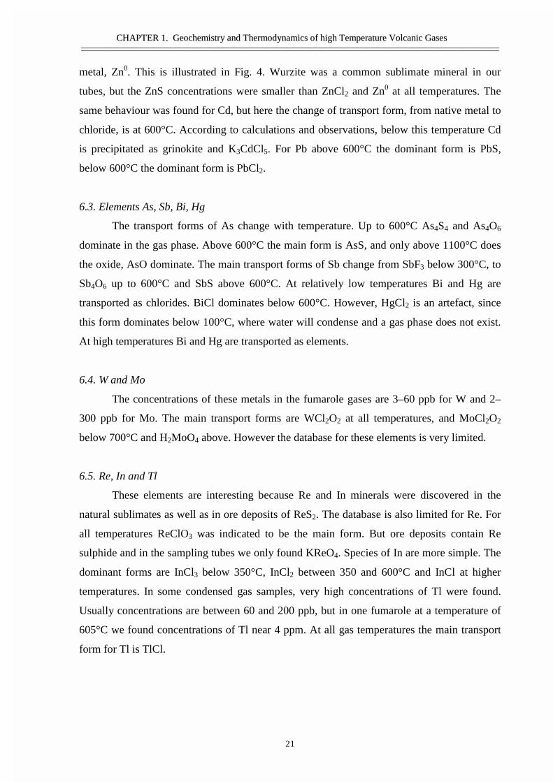
Fig. 5. Transport species of silicon at high temperatures and 1 bar (Shmulovich, et al., 1997) calculatedfor single homogeneous fluid phase using the database IVTANTERMO. Only seven species whichhave a concentration greater than 10-10 are presented. At T >750°C the main transport species is siliconmonoxide (SiO).
6.6. Si and Al
These elements are the most interesting since they were found as native elements in
natural sublimates and in the sampling tubes. The result of thermodynamic modelling for the
Si species in a gas phase at 1 bar is presented in Fig. 5 (Shmulovich, et al., 1997). At
temperatures below 750°C, the main transport form is SiCl4. SiF4 concentrations are an order
of magnitude smaller. Above 750°C the main transport form is monoxide, SiO, and to a lesser
extent SiO2. Transport of this element in the subvalency state is quite usual for chemical
transport reactions (Schafer, 1964), but as far as we know this has never been proposed for
natural hydrothermal fluids. These results give the key to the understanding of the process of
native element formation at high oxygen fugacity. As silicon monoxide does not have a solid
state, the cooling of the gas must lead to the precipitation of excess Si. Normally, the SiO2
would be precipitated and at high temperatures we observe perfect crystal polymorphs of
tridimite or cristobalite, sometime with aegirine needles. But, if salts were precipitated
beforehand and formed salt melt drops on the wall of the sampling tube or gas conduits, the
disproportionation reaction could be realised on the surface of the drops. The reaction 2SiO =
SiCl4 SiOSiF4
SiS 2
SiO2
SiS
SiCl2
600 700 800 900
-3
-5
-7
-9
-11
Temperature, ˚C
log
Xi
CCHHAAPPTTEERR 11.. GGeeoocchheemmiissttrryy aanndd TThheerrmmooddyynnaammiiccss ooff hhiigghh TTeemmppeerraattuurree VVoollccaanniicc GGaasseess————————————————————————————————————————————————————————————————————————————————————————————————————————————————
23
Si + SiO2 can precipitate native Si if the Si is protected from oxidation via an oxygen-free
medium. Under the protection of a salt melt or salt crystals the metal can remain unoxidized
after cooling. We really observed these native metals (Al, Si) in salt ‘shirts’. Experiments with
salt traps on the high-temperature fumaroles, analysed by electron microprobe after the salt
mixture (NaCl + KCl) was washed out, showed a rest powder with a Si/O ratio of 1:1. The
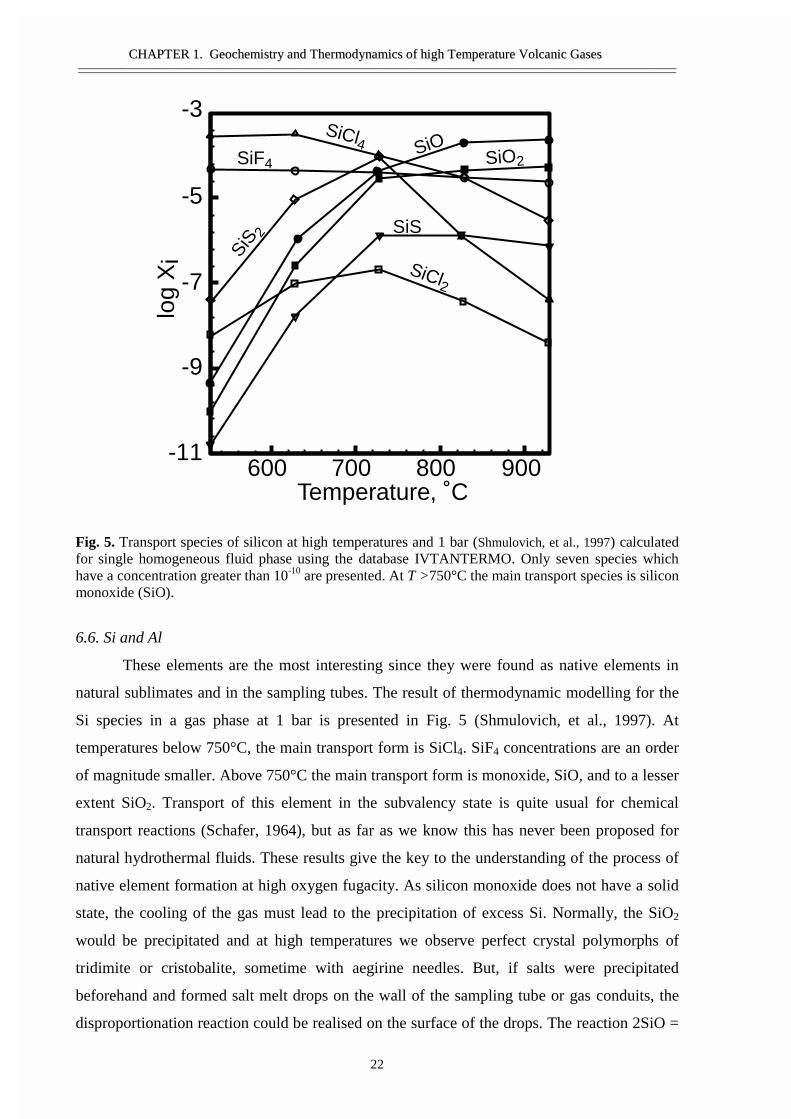
transport forms of Al from calculations is inconsistent with the sublimate mineralogy Fig. 6.
At temperatures below 700°C the main form is NaAlF4 (or KAlF4, dependent on
Fig. 6. The principal transport forms for Al in the fumarole gas, as in Fig. 3 and Fig. 4. Four mainspecies of 134 which were included in a minimisation procedure are presented. Al has a normalvalence of 3+ in all these species, none of which can precipitate the native metal.
the K/Na ratio), and above 700°C Al(OH)3. Our database contained 134 Al species, which
were included in the procedure of minimisation of the Gibbs free energy (Shvarov, 1988). The
diagram in Fig. 6 shows the four main forms; all others have negligible concentrations. The
main Al transport forms in this diagram look quite reasonable but we could not get the native
metals from these species. Yet we found more than fifteen Al particles in the sampling tubes
as a natural sublimate on the Kudriavy volcano and many of them have been described in the
literature (review in Novgorodova, 1983). Perhaps the precision of the thermodynamic
Al(OH) 3
NaAlF4
AlClF 2
AlC
l 3
Temperature, ˚C200 400 600 800 1000 1200
-25
-23
-21
-19
-17
-15
-13
-11
log
Xi
CCHHAAPPTTEERR 11.. GGeeoocchheemmiissttrryy aanndd TThheerrmmooddyynnaammiiccss ooff hhiigghh TTeemmppeerraattuurree VVoollccaanniicc GGaasseess————————————————————————————————————————————————————————————————————————————————————————————————————————————————
24
database that we used is not enough, or this process does not depend on the main forms but on
Al species which have concentrations some orders of magnitude lower than the main species.
This last version does not seem reasonable. Very rough calculations for NaCl and KCl
suggest that 0.5% of the amount that theoretically goes through the tubes should precipitate. If
AlCl0 has a concentration of 5 orders of magnitude below Al(OH)3 , it would be very difficult
to determine the quantity of the disproportionation products.
7. Mass transport by gases
During the 1995 field season on the Kudriavy volcano COSPEC measurements were
done by S. Williams and T. Fisher (Arizona State University, pers. commun., 1995). The bulk
emission of magmatic gases was estimated at about 2000 metric tons per day. Surface
mapping of the fumarole fields and measurement of gas velocities in the jets and in the steam
areas have suggested that this value is an order of magnitude higher. However, these
measurements have included meteoric as well as magmatic water. In fact, the correlation
spectrometer (COSPEC) measured the diminution of sky ultraviolet radiation by SO2, and the
total emission of magmatic gases was calculated from the ratio of SO2/H2O in the hottest
fumaroles which is more representative of magmatic gas. From analyses of condensed gases it
follows that metal concentrations do not depend on the temperatures of the fumaroles as long
as temperatures are above 350°C. This means, that calculations involving element exchanging
could increase by one order of magnitude if we take into account the remobilization of
elements by meteoric water.
The total quantity of the elements which were transported via the gas phase from the
magma chamber after the last explosion in 1883 has been calculated as a minimal value and
can be increased one order of magnitude. These values in metric tons are: for halogens Cl
2·107, Br 1.5·103, I 4.5·103; for the ore metals Cu 45, Pb 620, Zn 500, Sn 80, W 25, Mo 90, Se
65, As 450, Hg 20, Tl 110 and Bi 60.
Of course, the majority of these elements and their compounds dissolve in ocean water
and the contribution of passive volcanic gas emission to the atmosphere is not as important as
that of industrial emission and catastrophic explosions. However, in order to understand the
sequence of formation of ore deposits, we must also take into account L–V fractionation and
gas transport as the model is developed.
CCHHAAPPTTEERR 11.. GGeeoocchheemmiissttrryy aanndd TThheerrmmooddyynnaammiiccss ooff hhiigghh TTeemmppeerraattuurree VVoollccaanniicc GGaasseess————————————————————————————————————————————————————————————————————————————————————————————————————————————————
25
8. Conclusions
Long-term investigations of sublimate precipitation of main and trace elements using
optic, SEM and microprobe studies, analysis of volcanic gases and geochemical modelling of
transport forms have been carried out on the Kudriavy volcano, which produces
approximately 2000 tons/day of magmatic gases. The sublimates precipitated in quartz glass
tubes as practically monomineral clusters. This process could be a model for industrial
technologies to separate toxic, rare and heavy metals from waste. These low-density gases
transport elements at high T and low P mainly as halogenides and/or as hydroxides. Some of
the elements have a low valency state, and can be precipitated by regulation of the oxygen
fugacity.
The transport forms for many elements which were produced by geochemical
modelling of a real volcanic gas have very much in common with the list of first species
which condensed out of the protosolar nebula at the beginning of the formation of our star
(Word, 1976). In interplanetary space, at high temperatures (1200–2000 K) and low densities
(low pressures), the same species were produced as the ones found in volcanic gases
according to our calculations. This suggests that perhaps the process of sublimate formation
could be used as an experimental model for the formation of more complex molecules and
crystalline phases in the nebula as well.
Acknowledgements
We are thankful for the support of the fieldwork on the Kudriavy volcano by the
Russian Fund of Basic Investigations, the Russian Ministry of Sciences and Technology and,
furthermore, the organising committee of the Geochemical Engineering Symposium for the
opportunity to participate. Many thanks to Daniel Harlov and Hans Zijlstra for corrections of
our terrible English.
References
Bischoff, J.L., Pitzer, K.S., 1989. Liquid–vapor relations for the system NaCl–H2O: summary
of the PTX surface from 300 to 500°C. Am. J. Sci 289, 217–248.
CCHHAAPPTTEERR 11.. GGeeoocchheemmiissttrryy aanndd TThheerrmmooddyynnaammiiccss ooff hhiigghh TTeemmppeerraattuurree VVoollccaanniicc GGaasseess————————————————————————————————————————————————————————————————————————————————————————————————————————————————
26
Bischoff, J.L., Rosenbauer, R.J., Fournier, R.O., 1996. The generation of HCl in the system
CaCl2–H2O: vapor–liquid relations from 380–500°. Geochim. Cosmochim. Acta 60,
7–16.
Bodnar, R.J., Burnham, C.W., Sterner, S.M., 1985. Synthetic fluid inclusions in natural
quartz, III. Determination of phase equilibrium properties in the system H2O–NaCl to
1000° and 1500 bars. Geochim. Cosmochim. Acta 49, 1861–1873.
Glushko, V.P. (Editor), 1978–1982. Thermodynamic Properties of Individual Matters.
Moscow, v. 1–4, (Database IVTANTERMO).
Keppler, H., 1989. The influence of the fluid phase composition on the solidus temperatures
in the haplogranite system NaAlSi3O8–KalSi3O8–SiO2–H2O–CO2. Contrib. Mineral.
Petrol. 102, 321–327.
Khitarov, N.I., 1954. Chlorides of sodium and calcium as a possible source of acid media at
depth. Dokl. Akad. Nauk SSSR 94 (3), 519–521.
Korzhinsky, M.A., Tkachenko, S.I., Shmulovich, K.I., Taran, Y.A., Steinberg, G.S., 1994.
Discovery of a pure rhenium mineral at Kudriavy volcano. Nature 369 (6475), 51–52.
Korzhinsky, M.A., Tkachenko, S.I., Shmulovich, K.I., Steinberg, G.S., 1995. Native Al and
Si formation. Nature 375 (6532), 544.
Korzhinsky, M.A., Tkachenko, S.I., Bulgakov, R.F., Shmulovich, K.I., 1996. Condensate
compositions and native metals in sublimates of high temperature gas streams of
Kudriavyi volcano, Iturup Island (Kuril Islands). Geochem. Int. 34 (12), 1175–1182.
Novgorodova, M.I., 1983. Native Metals in Hydrothermal Ores. Nauka, Moscow, 287 pp.
Novgorodova, M.I., 1996. Native magnesium and the problem of its genesis. Geochem. Int.
34 (1), 36–44.
Pitzer, K.S., Pabalan, R.T., 1986. Thermodynamics of NaCl in steam. Geochim. Cosmochim.
Acta 50, 1445–1454.
Quisefit, J.P., Toutain, J.P., Bergametti, G., Javoy, M., Cheynet, B., Person, A., 1989.
Evolution versus cooling of gaseous volcanic emission from Momotombo volcano,
Nicaragua thermochemical model and observations. Geochim. Cosmochim. Acta 53,
2591–2608.
Rosen, E., Osadchii, E., Tkachenko, S.I., 1993. Oxygen fugacity directly measured in
fumaroles of the volcano Kudriaviy Kuril Isles. Chem. Erde 53, 219–226.
Schafer, H., 1964. Chemische Transportreaktionen. Verlag Chemie, Weinhelm, Bergstr.
(Russian version: Mir, Moscow).
CCHHAAPPTTEERR 11.. GGeeoocchheemmiissttrryy aanndd TThheerrmmooddyynnaammiiccss ooff hhiigghh TTeemmppeerraattuurree VVoollccaanniicc GGaasseess————————————————————————————————————————————————————————————————————————————————————————————————————————————————
27
Schafer, H., 1981. Chemical transport reactions in gases and some remarks concerning melts
and fluid phases. In: Chemistry and Geochemistry of Solutions at High Temperatures
and Pressures, Proc. Nobel Sympos., Karlskoga, 1979, Phys. and Chem. Earth, pp.
409–417.
Schuiling, R.D., 1990. Geochemical engineering: some thoughts on a new research field.
Appl. Geochem. 5, 251–262.
Shmulovich, K.I., Vakulenko, A.G., Shiryaev, A.A., 1997. Formation of Native Silicon in
Sublimates of the Kudryavyi Volcano, Iturup Island, Kurils Islands, Dokl Ross. Akad.
Nauk, 354 (6), 800-803.
Shvarov, Y.V., 1988. Calculation of equilibrium compositions of the hydrogeochemical
system via Gibbs free energy minimization. In: Kraynov, S.R. (Ed.), Methods of
Geochemical Modeling and Forecasting in Hydrogeology(in Russian). Nedra, Moscow
Symonds, R.B., Reed, M.H., 1993. Calculation of multicomponent chemical equilibria in gas–
solid–liquid system: calculation methods, thermochemical data, and application to
studies of high-temperature volcanic gases with examples from Mount St. Helens. Am.
J. Sci. 293, 758–864.
Symonds, R.B., Reed, M.H., Rose, W.I., 1992. Origin, speciation and fluxes of trace element
gases at Augustino volcano, Alaska: insights into magma degassing and fumarole
processes. Geochim. Cosmochim. Acta 56, 633–657.
Taran, Y.A., Hedenquist, J.W., Korzhinsky, M.A., Tkachenko, S.I., Shmulovich, K.I., 1995.
Geochemistry of magmatic gases from Kudriavy volcano, Iturup, Kuril Islands.
Geochim. Cosmochim. Acta 59, 1749–1761.
Tkachenko, S.I., Shmulovich, K.I., 1992. Liquid–vapour equilibria in the system water–salt
NaCl, KCl, CaCl2, MgCl2 at 400–600°. Dokl. Akad. Nauk SSSR 326 (6), 1055–1059.
Vakulenko, A.G., Alekhin, Y.V., Razina, M.V., 1989. Solubility and thermodynamic
properties of alkali chlorides in steam. Proc. II Int. Symp. Properties of Water and
Steam, Prague, pp. 395–401.
Word, W.R., 1976. Formation of solar system. In: Avrett, E.A. Ed., Frontiers of Astrophysics.
Harvard University Press, Cambridge, pp. 10–48.
Evolution of Composition of High-Temperature Fumarolic Gases
from Kudryavy Volcano, Iturup, Kuril Islands:
Thermodynamic Modelling
CCHHAAPPTTEERR 11.. GGeeoocchheemmiissttrryy aanndd TThheerrmmooddyynnaammiiccss ooff hhiigghh TTeemmppeerraattuurree VVoollccaanniicc GGaasseess————————————————————————————————————————————————————————————————————————————————————————————————————————————————
29
Abstract
Based on the chemical analyses of gases and condensates from high-temperature
fumaroles of the Kudryavy volcano, we performed a thermodynamic simulation of
transportation and deposition of ore- and rock-forming elements in high-temperature volcanic
gases within a temperature range of 1373-373 K at 1 bar pressure. The results of our
numerical simulation of mineral deposition from gases are consistent with the data of field
observations. Alkali and alkali earth metals, Ga, In, Tl, Fe, Co, Ni, Cu, and Zn are mainly
transported as chlorides in the gas phase. Sulfide and chloride forms are characteristic of Ge,
Sn, Pb, and Bi at intermediate and low temperatures. Be, Al, and Si migrate as fluorides and
oxides, while As and Sb, as sulfides and oxides. More complex, oxyfluoride and oxychloride
species are typical of Ti, Zr, V, Mo, W, and Re. Cd (at high temperatures) and Hg (within the
whole temperature range) are transported in the neutral form. Our calculations revealed some
general regularities in the variation of element species in the gas phase at a low (1 bar)
pressure versus thermodynamic conditions.
CCHHAAPPTTEERR 11.. GGeeoocchheemmiissttrryy aanndd TThheerrmmooddyynnaammiiccss ooff hhiigghh TTeemmppeerraattuurree VVoollccaanniicc GGaasseess————————————————————————————————————————————————————————————————————————————————————————————————————————————————
30
High-temperature volcanic gases bear important information on the composition of
volatile components in shallow-level magma chambers. At present, the composition of
fumarolic gases from volcanoes in most of the geotectonic structures [1, 2, etc.] is well
known. H2O, CO2, SO2, H2S, HCl, and HF are main constituents of these gases. The content
of ore- and rock-forming elements in the condensates of volcanic gases usually ranges from 1
ppb to 10 ppm [3-7, etc.], which attests to their low solubility in the fluid and small
coefficients of their fractionation between the silicate melt and the gas phase at low pressure.
Studies of the volcanic sublimates [5, 7-11, etc.] resulted in the determination of their mineral
composition and thermal conditions of deposition of different components from gases flowing
in volcanic channels. However, knowledge of element species in volcanic gases is necessary
for understanding the processes operated on the gas cooling, deposition of solid phases, and
interaction between gases and surrounding rocks. The modern techniques for determining the
modes of element occurrence in gases and liquids are based on spectrometry. These
techniques are too complicated to be applied in the field investigations; that is why such data
are usually obtained through thermodynamic calculations. The calculations performed for
Momotombo [7], Augustine [12], and Mount St. Helens [13] volcanoes enabled to describe
quantitatively the processes and reactions in the volcanic gas-rock-sublimate system and to
determine the sources of different elements in the gas phase.
This paper presents the results of thermodynamic simulation of cooling of a high-
temperature gas in the Kudryavy volcano. The study was aimed at:
1. Construction of a physic-chemical model for transportation and deposition of substances
in the gas phase;
2. Comparison of the obtained results with the field data for checking the consistency of the
thermodynamic data and the correlation between the thermodynamic model and natural
process;
3. Calculation of the element species in the high-temperature fumarolic gases and
determination of general regularities in the gas transport.
THERMODYNAMIC MODEL
The following information is necessary for constructing a thermodynamic model that
approximates the changes in the composition of fumarolic gases during their cooling and the
deposition of solid phases from the supersaturated gases:
1. Complete chemical composition of the gases including major components and trace
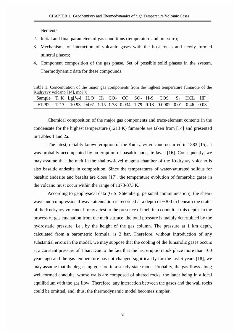
CCHHAAPPTTEERR 11.. GGeeoocchheemmiissttrryy aanndd TThheerrmmooddyynnaammiiccss ooff hhiigghh TTeemmppeerraattuurree VVoollccaanniicc GGaasseess————————————————————————————————————————————————————————————————————————————————————————————————————————————————
31
elements;
2. Initial and final parameters of gas conditions (temperature and pressure);
3. Mechanisms of interaction of volcanic gases with the host rocks and newly formed
mineral phases;
4. Component composition of the gas phase. Set of possible solid phases in the system.
Thermodynamic data for these compounds.
Table 1. Concentration of the major gas components from the highest temperature fumarole of theKudryavy volcano [14], mol %
Sample T, K Lg[fO2] H2O H2 CO2 CO SO2 H2S COS S2 HCL HF
F1292 1213 -10.93 94.61 1.15 1.78 0.034 1.79 0.18 0.0002 0.01 0.46 0.03
Chemical composition of the major gas components and trace-element contents in the
condensate for the highest temperature (1213 K) fumarole are taken from [14] and presented
in Tables 1 and 2a.
The latest, reliably known eruption of the Kudryavy volcano occurred in 1883 [15]; it
was probably accompanied by an eruption of basaltic andesite lavas [16]. Consequently, we
may assume that the melt in the shallow-level magma chamber of the Kudryavy volcano is
also basaltic andesite in composition. Since the temperatures of water-saturated solidus for
basaltic andesite and basalts are close [17], the temperature evolution of fumarolic gases in
the volcano must occur within the range of 1373-373 K.
According to geophysical data (G.S. Shteinberg, personal communication), the shear-
wave and compressional-wave attenuation is recorded at a depth of ~300 m beneath the crater
of the Kudryavy volcano. It may attest to the presence of melt in a conduit at this depth. In the
process of gas emanation from the melt surface, the total pressure is mainly determined by the
hydrostatic pressure, i.e., by the height of the gas column. The pressure at 1 km depth,
calculated from a barometric formula, is 2 bar. Therefore, without introduction of any
substantial errors in the model, we may suppose that the cooling of the fumarolic gases occurs
at a constant pressure of 1 bar. Due to the fact that the last eruption took place more than 100
years ago and the gas temperature has not changed significantly for the last 6 years [18], we
may assume that the degassing goes on in a steady-state mode. Probably, the gas flows along
well-formed conduits, whose walls are composed of altered rocks, the latter being in a local
equilibrium with the gas flow. Therefore, any interaction between the gases and the wall rocks
could be omitted, and, thus, the thermodynamic model becomes simpler.
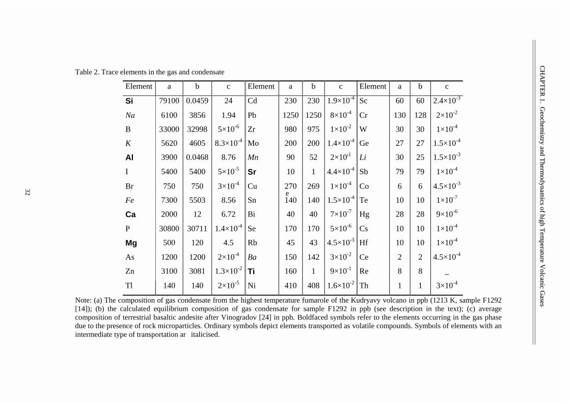
C CH H
A AP P
T TE E
R R 1 1. . G G
e eo oc ch he em mi is st tr ry y a an nd d T T
h he er rm mo od dy yn na am m
i ic cs s o of f h hi ig gh h T Te em m
p pe er ra at tu ur re e V Vo ol lc ca an ni ic c G G
a as se es s— —
— —— —
— —— —
— —— —
— —— —
— —— —
— —— —
— —— —
— —— —
— —— —
— —— —
— —— —
— —— —
— —— —
— —— —
— —— —
— —— —
— —— —
— —— —
— —— —
— —— —
— —— —
— —— —
— —— —
— —— —
— —— —
— —— —
— —— —
— —
32
Table 2. Trace elements in the gas and condensate
Element a b c Element a b c Element a b c
Si 79100 0.0459 24 Cd 230 230 1.9×10⁻⁴ Sc 60 60 2.4×10⁻³
Na 6100 3856 1.94 Pb 1250 1250 8×10⁻⁴ Cr 130 128 2×10⁻²
B 33000 32998 5×10⁻⁶ Zr 980 975 1×10⁻² W 30 30 1×10⁻⁴
K 5620 4605 8.3×10⁻⁴ Mo 200 200 1.4×10⁻⁴ Ge 27 27 1.5×10⁻⁴
Al 3900 0.0468 8.76 Mn 90 52 2×10'1 Li 30 25 1.5×10⁻³
I 5400 5400 5×10⁻⁵ Sr 10 1 4.4×10⁻⁴ Sb 79 79 1×10⁻⁴
Br 750 750 3×10⁻⁴ Cu 270 269 1×10⁻⁴ Co 6 6 4.5×10⁻³
Fe 7300 5503 8.56 Sn 140 140 1.5×10⁻⁴ Te 10 10 1×10⁻⁷
Ca 2000 12 6.72 Bi 40 40 7×10⁻⁷ Hg 28 28 9×10⁻⁶
P 30800 30711 1.4×10⁻⁴ Se 170 170 5×10⁻⁶ Cs 10 10 1×10⁻⁴
Mg 500 120 4.5 Rb 45 43 4.5×10⁻³ Hf 10 10 1×10⁻⁴
As 1200 1200 2×10⁻⁴ Ba 150 142 3×10⁻² Ce 2 2 4.5×10⁻⁴
Zn 3100 3081 1.3×10⁻² Ti 160 1 9×10⁻¹ Re 8 8 _
Tl 140 140 2×10⁻⁵ Ni 410 408 1.6×10⁻² Th 1 1 3×10⁻⁴
Note: (a) The composition of gas condensate from the highest temperature fumarole of the Kudryavy volcano in ppb (1213 K, sample F1292[14]); (b) the calculated equilibrium composition of gas condensate for sample F1292 in ppb (see description in the text); (c) averagecomposition of terrestrial basaltic andesite after Vinogradov [24] in ppb. Boldfaced symbols refer to the elements occurring in the gas phasedue to the presence of rock microparticles. Ordinary symbols depict elements transported as volatile compounds. Symbols of elements with anintermediate type of transportation ar
e
italicised.
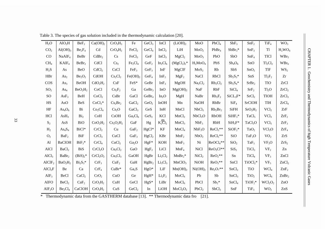
C CH H
A AP P
T TE E
R R 1 1. . G G
e eo oc ch he em mi is st tr ry y a an nd d T T
h he er rm mo od dy yn na am m
i ic cs s o of f h hi ig gh h T Te em m
p pe er ra at tu ur re e V Vo ol lc ca an ni ic c G G
a as se es s— —
— —— —
— —— —
— —— —
— —— —
— —— —
— —— —
— —— —
— —— —
— —— —
— —— —
— —— —
— —— —
— —— —
— —— —
— —— —
— —— —
— —— —
— —— —
— —— —
— —— —
— —— —
— —— —
— —— —
— —— —
— —— —
— —— —
— —— —
— —
33
Table 3. The species of gas solution included in the thermodynamic calculation [20].
H2O AlO2H BeF2 Ca(OH)2 CrO3H3 Fe GeCl3 InCl (LiOH)2 MoO PbCl4 SbF3 SnF2 TiF4 WO3
CO2 Al(OH)3 Be2F4 Cd CrO4H2 FeCl2 GeCl4 InCl2 LiH MoO2 PbBr4 SbBr3* SnF3 Tl H2WO4
CO NaAlF4 BeBr CdBr2 Cs FeCl3 GeF InCl3 MgCl2 MoO3 PbO SbO SnF4 TlCl WBr5
CH4 KAlF4 BeBr2 CdCl Cs2 Fe2Cl4 GeF2 In2Cl6 (MgCl2)2* H2MoO4 PbS Sb4O6 SnO Tl2Cl2 WBr6
H2S As BeO CdCl2 CsCl FeF3 GeF3 InF MgClF MoS2 Rb SbS SnO2 TlF WS2
HBr As2 Be2O2 CdOH Cs2Cl2 Fe(OH)2 GeF4 InF2 MgF2 NaCl RbCl Sb2S3* SnS Tl2F2 Zr
COS As3 BeOH CdO2H2 CsF FeS* GeBr InF3 MgOH Na2Cl2 Rb2Cl2 Sb2S4* SrBr2 TlO ZrCl
SO2 As4 BeO2H2 CoCl Cs2F2 Ga GeBr3 InO Mg(OH)2 NaF RbF SiCl4 SrF2 Tl2O ZrCl2
SO AsF3 BeH CoCl2 CsBr GaCl GeBr4 In2O MgH NaBr Rb2F2 SiCL3F* SrCl2 TlOH ZrCl3
HS AsO BeS CoCl3* Cs2Br2 GaCl2 GeO2 InOH Mn NaOH RbBr SiF4 SrClOH TlH ZrCl4
HF As4O6 Bi Co2Cl4 Cs2O GaCl3 GeS InH MnCl NbCl5 Rb2Br2 SiFH SrO2H2 VCl2 ZrF
HCl AsH3 Bi2 CoH CsOH Ga2Cl6 GeS2 KCl MnCl2 NbCl3O RbOH SiHF3* TaCl5 VCl3 ZrF2
S2 AsS BiO CoO2H2 Cs2O2H2 GaF Hg K2Cl2 MnCl3 NbF5 RbH SiH3F* TaCl3O VCl5 ZrF3
H2 As4S4 BiCl* CrCl2 Cu GaF2 HgCl* KF MnCl4 NbF3O ReCl3** SiOF2* TaO2 VCl3O ZrF4
O2 BaF2 BiF CrCl3 CuCl GaF3 HgCl2 KBr MnF2 NbO2 ReCl5** SiO TaF3O VO2 ZrS
Al BaClOH BiF3* CrCl4 CuCl2 Ga2O HgF* KOH MnF3 Ni ReOCl4** SiO2 TaF5 VF3O ZrS2
AlCl BaCl2 BiS CrCl2O Cu2Cl2 GaO HgF2 LiCl MnF4 NiCl ReO3Cl** SiS2 TiCl3 VF2 Zn
AlCl3 BaBr2 (BiS)2* CrCl2O2 Cu3Cl3 GaOH HgBr Li2Cl2 MnBr2* NiCl2 ReO2** Sn TiCl4 VF3 ZnCl
AlClF2 BaO2H2 Bi2S3* CrF3 CuF2 GaH HgBr2 Li3Cl3 MnClO3 NiOH ReO3** SnCl TiOCl2* VF5 ZnCl2
AlCl2F Be Ca CrF4 CuBr* Ga2S HgO* LiF Mn(OH)2 Ni(OH)2 Re2O7** SnCl2 TiO WCl4 ZnF2
AlF3 BeCl CaCl2 CrO2 CuO Ge HgH* Li2F2 MoCl4 Pb Sb SnCl3 TiO2 WCl6 ZnBr2
AlFO BeCl2 CaF2 CrO2H2 CuH GeCl HgS* LiBr MoCl6 PbCl Sb2* SnCl4 TiOF2* WCl2O2 ZnO
AlF2O Be2Cl4 CaClOH CrO3H2 CuS GeCl2 In LiOH MoCl2O2 PbCl2 SbCl3 SnF TiF3 WO2 ZnS
* Thermodynamic data from the GASTHERM database [13]. ** Thermodynamic data fro
m
[21].

CCHHAAPPTTEERR 11.. GGeeoocchheemmiissttrryy aanndd TThheerrmmooddyynnaammiiccss ooff hhiigghh TTeemmppeerraattuurree VVoollccaanniicc GGaasseess————————————————————————————————————————————————————————————————————————————————————————————————————————————————
34
CALCULATION TECHNIQUES AND THERMODYNAMIC DATA
The modelling has been performed using the GBGAS program (the author is Dr. D.V.
Grichuk, Moscow State University) for calculating heterogeneous equilibria of gas solution
with phases of constant composition. The program permits a calculation of gas composition in
equilibrium with the phases of constant composition at a given temperature, pressure and bulk
system composition. It is assumed for calculation that gas phase is always present in the
system and the set of equilibrium phases of constant composition is estimated by
minimisation of the system free energy. This program is capable of simultaneously operating
with no more than 500 compounds of 50 elements, and no more than 400 compounds being
gas species.
The isobaric cooling of the gas phase was modelled using the procedure of flow
reactor [19]. In this technique, the continuous cooling of a thermodynamic system is
approximated by a combination of isothermal steps (flow reactors). For each step, the mineral
assemblage being in equilibrium with the gas phase is calculated at a given temperature and
bulk system composition. This mineral assemblage (solid phase) is eliminated from the
system and the equilibrium gas phase is taken as the bulk system composition for the next
step of calculation, i.e., in a reactor of lower temperature. This procedure was applied for
calculating the composition of equilibrium gas mixtures and distribution of volatile species
and mineral assemblages originated during the cooling of the initial gas composition (Table
2b) from 1373 to 373 K. The calculation step was adopted at 20 K.
The calculations were fulfilled using the IVTAN-TERMO thermodynamic database
[20]. Some additional data were taken from [13, 21, 22]. The calculation involved over 1700
gas species and 1500 solid phases for 82 elements.
Since the amount of the thermodynamic data substantially exceeded the value
appropriate to the computer program, only the most important gas species for many elements
were preliminarily chosen. The total concentrations of H, O, S, C, Cl and F, which form
volatile compounds with trace elements and serve as transport agents in volcanic gas, are
several orders of magnitude greater than the other element contents. Therefore, the trace
elements, which do not form complex volatile compounds in the gas phase, were supposed to
not mutually influence the distribution of gas species and could be considered, as the first
approximation, independently of one another.
Such an approach made it possible to subdivide the whole task into a series of subtasks
involving 18 elements with all their thermodynamic properties taken into account.
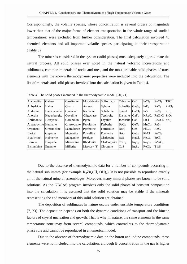
CCHHAAPPTTEERR 11.. GGeeoocchheemmiissttrryy aanndd TThheerrmmooddyynnaammiiccss ooff hhiigghh TTeemmppeerraattuurree VVoollccaanniicc GGaasseess————————————————————————————————————————————————————————————————————————————————————————————————————————————————
35
Correspondingly, the volatile species, whose concentration is several orders of magnitude
lower than that of the major forms of element transportation in the whole range of studied
temperatures, were excluded from further consideration. The final calculation involved 45
chemical elements and all important volatile species participating in their transportation
(Table 3).
The minerals considered in the system (solid phases) must adequately approximate the
natural process. All solid phases ever noted in the natural volcanic incrustations and
sublimates, common minerals of rocks and ores, and the most probable solid phases of trace
elements with the known thermodynamic properties were included into the calculation. The
list of minerals and solid phases involved into the calculation is given in Table 4.
Table 4. The solid phases included in the thermodynamic model [20, 21]
Alabandite Galena Cassiterite Molybdenite Sulfur (s,l) Celestite CsCl InCl3 ReCl5 T1C1
Anhydride Halite Quartz Arsenic Sylvite Scheelite Ga2S3 InF3 ReO2 ZnCl2
Andesine Hausmannite Cinnabar Niccolite Sphalerite Spinel GaCI3 InS ReO3 ZrF4
Anortite Hedenbergite Covellite Oligoclase Tephroite Enstatite GaF3 KReO4 ReO3Cl ZrO2
Antimonite Hercynite Corundum Pyrite Fayalite Jacobsite GaS LiCl ReOCl4 ZrS2
Arsenopyrite Hematite Crystobalite Pyrolusite Ferberite BeCl2 GeO2 MnCl2 ReS2
Orpiment Greenockite Labradorite Pyrrhotite Ferrosilite BeF2 GeS PbCl2 ReS3
Barite Gypsum Magnetite Powellite Forsterite BeO GeS2 RbCl SnCl2
Bytownite Hubnerite Manganite Realgar Chalcocite BeS HgCl2 Re2O7 SrCl2
Bornite Diopside Microcline Rhodonite Chalcopyrite CdCl2 In2S3 Re2S7 SrWO4
Bismuthine Ilmenite Millerite Mercury (1) Chromite CoS In5S6 ReCl3 T12S
Due to the absence of thermodynamic data for a number of compounds occurring in
the natural sublimates (for example K3Zn2(Cl, OH)7), it is not possible to reproduce exactly
all of the natural mineral assemblages. Moreover, many mineral phases are known to be solid
solutions. As the GBGAS program involves only the solid phases of constant composition
into the calculation, it is assumed that the solid solution may be stable if the minerals
representing the end members of this solid solution are obtained.
The deposition of sublimates in nature occurs under unstable temperature conditions
[7, 23]. The deposition depends on both the dynamic conditions of transport and the kinetic
factors of crystal nucleation and growth. That is why, in nature, the same elements in the same
temperature zone may form several compounds, which contradicts to the thermodynamic
phase rule and cannot be reproduced in a numerical model.
Due to the absence of thermodynamic data on the boron and iodine compounds, these
elements were not included into the calculation, although B concentration in the gas is higher
CCHHAAPPTTEERR 11.. GGeeoocchheemmiissttrryy aanndd TThheerrmmooddyynnaammiiccss ooff hhiigghh TTeemmppeerraattuurree VVoollccaanniicc GGaasseess————————————————————————————————————————————————————————————————————————————————————————————————————————————————
36
than the content of all other trace elements and the I content is comparable with the total
concentration of all ore elements.
When calculating, any precipitation of solid phase is registered, including its mole
fraction in the system as low as 1E-18. In the natural conditions, the deposition of solid
phases at their very low concentrations in the system becomes impossible due to the kinetic
factors. In addition, the mineral phase occurring in sublimates in small amounts may be
missed in the microprobe analysis. Because of that, the description of the calculation results
includes the data only for elements and compounds identified in the natural sublimates.
THERMODYNAMIC ANALYSIS OF GAS AND CONDENSATE COMPOSITION
In order to develop a correct model of evolution of the volcanic gas composition, one
has to determine whether the species of the gas phase are in thermodynamic equilibrium at the
temperature of sampling. The processes of oxidation of gas species, condensation and/or
boiling at the time of sampling, as well as errors of analysis result in errors in determination
of the original gas composition. Therefore, the composition of most of the analysed volcanic
gases is not in equilibrium at the temperature of sampling. However, if contamination is low
and analytical errors are small, it is often possible to restore the proportions of major gas
species corresponding to the last moment of thermodynamic equilibrium in the gas phase.
Such a procedure applied for reconstruction of the Kudryavy volcano gas composition is
comprehensively presented in [14]. For further calculations, we used the highest temperature
gas composition (sample F1292) restored in [14] (Table 1, 2a), as the initial gas composition
for major components.
Table 5. The composition of basaltic andesites of the Kudryavy volcano [16], wt %
SiO2 TiO2 Al2O3 FeO MnO MgO CaO Na2O K2O55.2 0.58 19.96 6.52 0.15 2.93 7.81 2.56 0.7
The same technique of correcting the gas composition, unfortunately, cannot be
applied to minor components, where analytical errors may influence the calculation results. It
is suggested [5, 12, 13] that most of Ca, Al, Mg and some of Mn, Fe, Na, and K is transported
in the gas phase as the finest solid dust particles. These particles are involved in samples of
condensate together with the gas phase, which results in their overestimated contents. The true
gas composition can be calculated for the condition of equilibrium between the fluid and
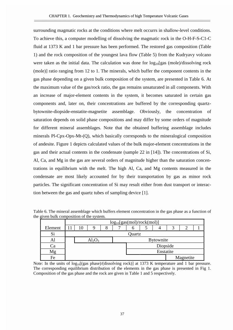
CCHHAAPPTTEERR 11.. GGeeoocchheemmiissttrryy aanndd TThheerrmmooddyynnaammiiccss ooff hhiigghh TTeemmppeerraattuurree VVoollccaanniicc GGaasseess————————————————————————————————————————————————————————————————————————————————————————————————————————————————
37
surrounding magmatic rocks at the conditions where melt occurrs in shallow-level conditions.
To achieve this, a computer modelling of dissolving the magmatic rock in the O-H-F-S-C1-C
fluid at 1373 K and 1 bar pressure has been performed. The restored gas composition (Table
1) and the rock composition of the youngest lava flow (Table 5) from the Kudryavy volcano
were taken as the initial data. The calculation was done for log10[gas (mole)/dissolving rock
(mole)] ratio ranging from 12 to 1. The minerals, which buffer the component contents in the
gas phase depending on a given bulk composition of the system, are presented in Table 6. At
the maximum value of the gas/rock ratio, the gas remains unsaturated in all components. With
an increase of major-element contents in the system, it becomes saturated in certain gas
components and, later on, their concentrations are buffered by the corresponding quartz-
bytownite-diopside-enstatite-magnetite assemblage. Obviously, the concentration of
saturation depends on solid phase compositions and may differ by some orders of magnitude
for different mineral assemblages. Note that the obtained buffering assemblage includes
minerals Pl-Cpx-Opx-Mt-(Q), which basically corresponds to the mineralogical composition
of andesite. Figure 1 depicts calculated values of the bulk major-element concentrations in the
gas and their actual contents in the condensate (sample 22 in [14]). The concentrations of Si,
Al, Ca, and Mg in the gas are several orders of magnitude higher than the saturation concen-
trations in equilibrium with the melt. The high Al, Ca, and Mg contents measured in the
condensate are most likely accounted for by their transportation by gas as minor rock
particles. The significant concentration of Si may result either from dust transport or interac-
tion between the gas and quartz tubes of sampling device [1].
Table 6. The mineral assemblage which buffers element concentration in the gas phase as a function ofthe given bulk composition of the system.
log10[gas(mol)/rock(mol)]Element 11 10 9 8 7 6 5 4 3 2 1
Si QuartzAl Al2O3 BytowniteCa DiopsideMg EnstatiteFe Magnetite
Note: In the units of log10[(gas phase)/(dissolving rock)] at 1373 K temperature and 1 bar pressure.The corresponding equilibrium distribution of the elements in the gas phase is presented in Fig 1.Composition of the gas phase and the rock are given in Table 1 and 5 respectively.

CCHHAAPPTTEERR 11.. GGeeoocchheemmiissttrryy aanndd TThheerrmmooddyynnaammiiccss ooff hhiigghh TTeemmppeerraattuurree VVoollccaanniicc GGaasseess————————————————————————————————————————————————————————————————————————————————————————————————————————————————
38
Fig. 1. The results of modelling of dissolving the Kudryavy volcano basaltic andesite in the gas phaseat 1373 K temperature and 1 bar pressure. The boldfaced dashes designate mole fraction of rock-forming elements (italicized capital letters) in the volcanic gases from the highest temperature (1213K) fumarole, according to data of chemical analysis. The curves represent change of the elementconcentration in the gas phase versus the given bulk composition of the system in the units of log10[gas(mol)/rock (mol)]. At the maximum value of this ratio the gas dissolves the rock completely. Upon theincrease of rock proportion in the initial system composition, some elements of the gas phase becomesaturated. The equilibrium mineral assemblages buffering the gas composition in this case are given inTable 6.
In order to correct the minor-element composition of the gas, the contents of all
elements were subtracted from the condensate composition in proportion to their con-
centrations in basaltic andesite, so that the Ca, Al, and Mg contents become equal to the
Cl
Si
Mg
K
Al
Ca
F
C, S
Fe
Na
H O
Si
AlFe
MgCa
NaK
0
2
4
6
8
10
12
14024681012
The given system composition in unitsof log10[gas(mol)/rock(mol)]
-log
10[m
ole
frac
tion]
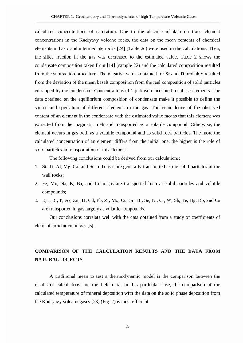
CCHHAAPPTTEERR 11.. GGeeoocchheemmiissttrryy aanndd TThheerrmmooddyynnaammiiccss ooff hhiigghh TTeemmppeerraattuurree VVoollccaanniicc GGaasseess————————————————————————————————————————————————————————————————————————————————————————————————————————————————
39
calculated concentrations of saturation. Due to the absence of data on trace element
concentrations in the Kudryavy volcano rocks, the data on the mean contents of chemical
elements in basic and intermediate rocks [24] (Table 2c) were used in the calculations. Then,
the silica fraction in the gas was decreased to the estimated value. Table 2 shows the
condensate composition taken from [14] (sample 22) and the calculated composition resulted
from the subtraction procedure. The negative values obtained for Sr and Ti probably resulted
from the deviation of the mean basalt composition from the real composition of solid particles
entrapped by the condensate. Concentrations of 1 ppb were accepted for these elements. The
data obtained on the equilibrium composition of condensate make it possible to define the
source and speciation of different elements in the gas. The coincidence of the observed
content of an element in the condensate with the estimated value means that this element was
extracted from the magmatic melt and transported as a volatile compound. Otherwise, the
element occurs in gas both as a volatile compound and as solid rock particles. The more the
calculated concentration of an element differs from the initial one, the higher is the role of
solid particles in transportation of this element.
The following conclusions could be derived from our calculations:
1. Si, Ti, Al, Mg, Ca, and Sr in the gas are generally transported as the solid particles of the
wall rocks;
2. Fe, Mn, Na, K, Ba, and Li in gas are transported both as solid particles and volatile
compounds;
3. B, I, Br, P, As, Zn, TI, Cd, Pb, Zr, Mo, Cu, Sn, Bi, Se, Ni, Cr, W, Sb, Te, Hg, Rb, and Cs
are transported in gas largely as volatile compounds.
Our conclusions correlate well with the data obtained from a study of coefficients of
element enrichment in gas [5].
COMPARISON OF THE CALCULATION RESULTS AND THE DATA FROM
NATURAL OBJECTS
A traditional mean to test a thermodynamic model is the comparison between the
results of calculations and the field data. In this particular case, the comparison of the
calculated temperature of mineral deposition with the data on the solid phase deposition from
the Kudryavy volcano gases [23] (Fig. 2) is most efficient.
CCHHAAPPTTEERR 11.. GGeeoocchheemmiissttrryy aanndd TThheerrmmooddyynnaammiiccss ooff hhiigghh TTeemmppeerraattuurree VVoollccaanniicc GGaasseess————————————————————————————————————————————————————————————————————————————————————————————————————————————————
40
Fig. 2. Comparison of the calculated data on the mineral deposition from the gas phase at a decreasingtemperature with the field observations [18, 23]. (1) Corresponds to the results of calculation, (2)shows the temperature interval of mineral deposition at natural conditions of Kudryavy volcano. Thecorresponding equilibrium compositions of the gas phase are presented on Fig. 3.
273 473 673 873 1073 1273T [K]
12

CCHHAAPPTTEERR 11.. GGeeoocchheemmiissttrryy aanndd TThheerrmmooddyynnaammiiccss ooff hhiigghh TTeemmppeerraattuurree VVoollccaanniicc GGaasseess————————————————————————————————————————————————————————————————————————————————————————————————————————————————
41
It should be noted that, due to the unstable temperature conditions while sampling
natural sublimates [23], a discrepancy in the temperature range of mineral stability between
the estimated values and those observed in nature must not be considered as a mistake up to
100 K. The sequence of mineral crystallisation with decreasing temperature is more
informative.
Silicates
According to the calculations, diopside is deposited within the temperature interval of
1323-1373K and is followed by forsterite at lower temperatures.
Natural silicates in the range of 1023-773K are represented by potassic feldspar,
clinopyroxene of augite-hedenbergite composition, and aegirine. Silicates (wollastonite,
grossular, sanidine) were also observed in the sublimates of a high-temperature zone in a
quartz pipe [11]. However, it was inferred in [23] that the presence of potassic feldspar and
pyroxenes could result from the transport and deposition of solid particles as discussed above.
Probably, crystallization of these silicates in nature should be expected at higher temperatures.
W and Mo Minerals
In our calculation, a joint deposition of scheelite and powellite (with the latter being
predominant) was simulated within the range of 993-893 K. In the natural sublimates,
scheelite, powellite, and their solid solutions also crystallized at temperatures of 1023-873 K.
From the calculation, molybdenite is stable at temperatures below 1043 K. In the
natural sublimates, molybdenite was observed within the whole range of temperatures from
1023 to 443 K. Its maximum precipitation occurs at 973-673 K, where MoS2 is a major phase.
The natural molybdenite contains small amounts of rhenium.
The hubnerite precipitation is simulated at temperatures below 763 K, while in the
natural sublimates, wolframite with Mn admixture is formed at temperatures of 1023-723 K.
Barite and Anhydrite
From the calculation, the deposition of barite occurs at temperatures below 1133 K. In
the natural sublimates, small amounts of BaSO4 were registered in a wide range of
temperatures from 1023 to 573K.
CCHHAAPPTTEERR 11.. GGeeoocchheemmiissttrryy aanndd TThheerrmmooddyynnaammiiccss ooff hhiigghh TTeemmppeerraattuurree VVoollccaanniicc GGaasseess————————————————————————————————————————————————————————————————————————————————————————————————————————————————
42
According to the calculation, anhydrite forms in the range of 1073-1013 and below
893 K. Within the range of 1013-893 K, anhydrite deposition ceases, because most of Ca
precipitates in CaWO4 and CaMoO4. In nature, small amounts of anhydrite were found in the
temperature range of 1023-773 K, together with scheelite and powellite.
Halite and Sylvite
According to the calculation, halite and sylvite crystallize together within the range of
873-373 K. The KC1 concentration in the sublimates is higher than that of NaCl, excluding
the temperature interval from 853 to 873 K. Under natural conditions, deposition of halite and
sylvite was noted within the whole temperature range of 1023-443 K, with the maximum
content at 923-673 K. A neutron activation analysis revealed that Na concentration in the
sublimates (and, correspondingly, NaCl as the major Na-bearing phase) at temperatures of
1023-823 K is higher than that of K (KC1).
Fe and Cu Minerals
According to the calculation, magnetite is stable at temperatures of 1353-773 K, while
in the natural sublimates only hematite was found in the range of 1023-823 K. In the gas
sublimates from other volcanoes, either magnetite [5, 7, 10] or magnetite and hematite [9, 25]
were observed. Forms of iron oxide deposition depend on the redox conditions in the gas
phase. The oxygen fugacity in the Kudryavy volcano gases at these temperatures is close to
the NNO buffer [14, 26, 27], which excludes the deposition of hematite in an equilibrium
process. The possible reasons for forming Fe2O3 under natural conditions are discussed in
[23]. The fO2, values obtained in our calculation are between the NNO and HM mineral
buffers. Therefore, magnetite can be the only possible equilibrium form of iron oxide
deposition in thermodynamic calculation.
In our simulation, bornite precipitates at 1133-853 K and 653-573 K; chalcopyrite, at
temperatures of 833-673 K; pyrite, below 773 K; and coveline, below 553 K. In the natural
sublimates, the iron and copper minerals are deposited in the following sequence: pyrite - at
973-513 K with the maximum at 793-593 K; chalcopyrite - at 973-473 K with the maximum
at 843-573 K; unidentified complex Cu-Fe-Zn-Cd-Sn sulfides were found in vents with
temperatures below 593 K.
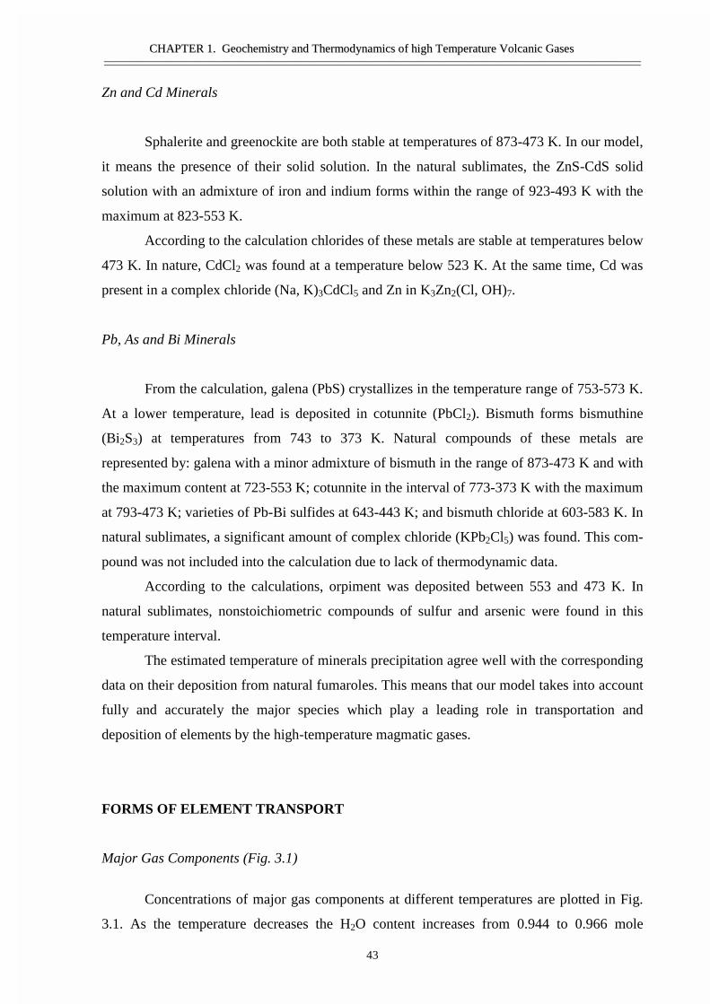
CCHHAAPPTTEERR 11.. GGeeoocchheemmiissttrryy aanndd TThheerrmmooddyynnaammiiccss ooff hhiigghh TTeemmppeerraattuurree VVoollccaanniicc GGaasseess————————————————————————————————————————————————————————————————————————————————————————————————————————————————
43
Zn and Cd Minerals
Sphalerite and greenockite are both stable at temperatures of 873-473 K. In our model,
it means the presence of their solid solution. In the natural sublimates, the ZnS-CdS solid
solution with an admixture of iron and indium forms within the range of 923-493 K with the
maximum at 823-553 K.
According to the calculation chlorides of these metals are stable at temperatures below
473 K. In nature, CdCl2 was found at a temperature below 523 K. At the same time, Cd was
present in a complex chloride (Na, K)3CdCl5 and Zn in K3Zn2(Cl, OH)7.
Pb, As and Bi Minerals
From the calculation, galena (PbS) crystallizes in the temperature range of 753-573 K.
At a lower temperature, lead is deposited in cotunnite (PbCl2). Bismuth forms bismuthine
(Bi2S3) at temperatures from 743 to 373 K. Natural compounds of these metals are
represented by: galena with a minor admixture of bismuth in the range of 873-473 K and with
the maximum content at 723-553 K; cotunnite in the interval of 773-373 K with the maximum
at 793-473 K; varieties of Pb-Bi sulfides at 643-443 K; and bismuth chloride at 603-583 K. In
natural sublimates, a significant amount of complex chloride (KPb2Cl5) was found. This com-
pound was not included into the calculation due to lack of thermodynamic data.
According to the calculations, orpiment was deposited between 553 and 473 K. In
natural sublimates, nonstoichiometric compounds of sulfur and arsenic were found in this
temperature interval.
The estimated temperature of minerals precipitation agree well with the corresponding
data on their deposition from natural fumaroles. This means that our model takes into account
fully and accurately the major species which play a leading role in transportation and
deposition of elements by the high-temperature magmatic gases.
FORMS OF ELEMENT TRANSPORT
Major Gas Components (Fig. 3.1)
Concentrations of major gas components at different temperatures are plotted in Fig.
3.1. As the temperature decreases the H2O content increases from 0.944 to 0.966 mole
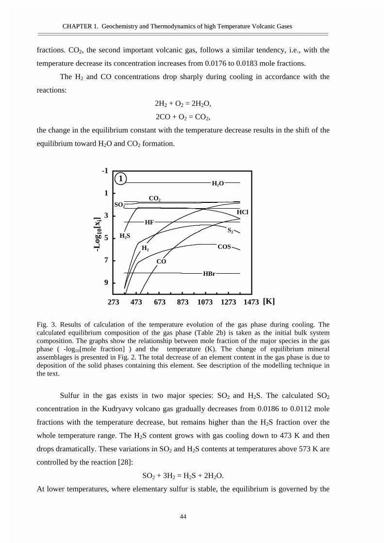
CCHHAAPPTTEERR 11.. GGeeoocchheemmiissttrryy aanndd TThheerrmmooddyynnaammiiccss ooff hhiigghh TTeemmppeerraattuurree VVoollccaanniicc GGaasseess————————————————————————————————————————————————————————————————————————————————————————————————————————————————
44
fractions. CO2, the second important volcanic gas, follows a similar tendency, i.e., with the
temperature decrease its concentration increases from 0.0176 to 0.0183 mole fractions.
The H2 and CO concentrations drop sharply during cooling in accordance with the
reactions:
2H2 + O2 = 2H2O,
2CO + O2 = CO2,
the change in the equilibrium constant with the temperature decrease results in the shift of the
equilibrium toward H2O and CO2 formation.
Fig. 3. Results of calculation of the temperature evolution of the gas phase during cooling. Thecalculated equilibrium composition of the gas phase (Table 2b) is taken as the initial bulk systemcomposition. The graphs show the relationship between mole fraction of the major species in the gasphase ( -log10[mole fraction] ) and the temperature (K). The change of equilibrium mineralassemblages is presented in Fig. 2. The total decrease of an element content in the gas phase is due todeposition of the solid phases containing this element. See description of the modelling technique inthe text.
Sulfur in the gas exists in two major species: SO2 and H2S. The calculated SO2
concentration in the Kudryavy volcano gas gradually decreases from 0.0186 to 0.0112 mole
fractions with the temperature decrease, but remains higher than the H2S fraction over the
whole temperature range. The H2S content grows with gas cooling down to 473 K and then
drops dramatically. These variations in SO2 and H2S contents at temperatures above 573 K are
controlled by the reaction [28]:
SO2 + 3H2 = H2S + 2H2O.
At lower temperatures, where elementary sulfur is stable, the equilibrium is governed by the
H2O
CO2
CO
H2S
HBr
COS
SO2
HF
HCl
S2
H2
-1
1
3
5
7
9
1
273 473 673 873 1073 1273 1473 [K]
-Log
10[x
i]
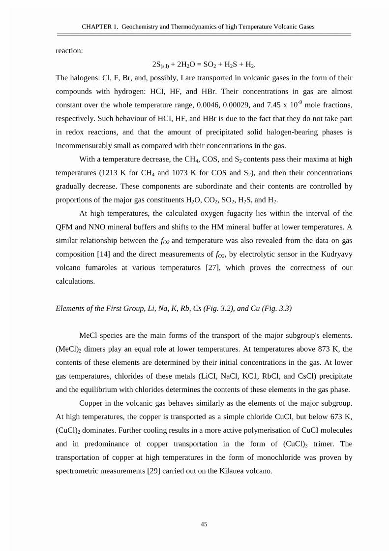
CCHHAAPPTTEERR 11.. GGeeoocchheemmiissttrryy aanndd TThheerrmmooddyynnaammiiccss ooff hhiigghh TTeemmppeerraattuurree VVoollccaanniicc GGaasseess————————————————————————————————————————————————————————————————————————————————————————————————————————————————
45
reaction:
2S(s,l) + 2H2O = SO2 + H2S + H2.
The halogens: Cl, F, Br, and, possibly, I are transported in volcanic gases in the form of their
compounds with hydrogen: HCI, HF, and HBr. Their concentrations in gas are almost
constant over the whole temperature range, 0.0046, 0.00029, and 7.45 x 10⁻⁹ mole fractions,
respectively. Such behaviour of HCI, HF, and HBr is due to the fact that they do not take part
in redox reactions, and that the amount of precipitated solid halogen-bearing phases is
incommensurably small as compared with their concentrations in the gas.
With a temperature decrease, the CH4, COS, and S2 contents pass their maxima at high
temperatures (1213 K for CH4 and 1073 K for COS and S2), and then their concentrations
gradually decrease. These components are subordinate and their contents are controlled by
proportions of the major gas constituents H2O, CO2, SO2, H2S, and H2.
At high temperatures, the calculated oxygen fugacity lies within the interval of the
QFM and NNO mineral buffers and shifts to the HM mineral buffer at lower temperatures. A
similar relationship between the fO2 and temperature was also revealed from the data on gas
composition [14] and the direct measurements of fO2, by electrolytic sensor in the Kudryavy
volcano fumaroles at various temperatures [27], which proves the correctness of our
calculations.
Elements of the First Group, Li, Na, K, Rb, Cs (Fig. 3.2), and Cu (Fig. 3.3)
MeCl species are the main forms of the transport of the major subgroup's elements.
(MeCl)2 dimers play an equal role at lower temperatures. At temperatures above 873 K, the
contents of these elements are determined by their initial concentrations in the gas. At lower
gas temperatures, chlorides of these metals (LiCI, NaCl, KC1, RbCl, and CsCl) precipitate
and the equilibrium with chlorides determines the contents of these elements in the gas phase.
Copper in the volcanic gas behaves similarly as the elements of the major subgroup.
At high temperatures, the copper is transported as a simple chloride CuCI, but below 673 K,
(CuCl)2 dominates. Further cooling results in a more active polymerisation of CuCI molecules
and in predominance of copper transportation in the form of (CuCl)3 trimer. The
transportation of copper at high temperatures in the form of monochloride was proven by
spectrometric measurements [29] carried out on the Kilauea volcano.
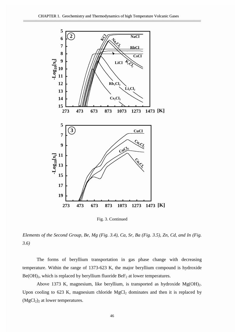
CCHHAAPPTTEERR 11.. GGeeoocchheemmiissttrryy aanndd TThheerrmmooddyynnaammiiccss ooff hhiigghh TTeemmppeerraattuurree VVoollccaanniicc GGaasseess————————————————————————————————————————————————————————————————————————————————————————————————————————————————
46
Fig. 3. Continued
Elements of the Second Group, Be, Mg (Fig. 3.4), Ca, Sr, Ba (Fig. 3.5), Zn, Cd, and In (Fig.
3.6)
The forms of beryllium transportation in gas phase change with decreasing
temperature. Within the range of 1373-623 K, the major beryllium compound is hydroxide
Be(OH)2, which is replaced by beryllium fluoride BeF2 at lower temperatures.
Above 1373 K, magnesium, like beryllium, is transported as hydroxide Mg(OH)2.
Upon cooling to 623 K, magnesium chloride MgCl2 dominates and then it is replaced by
(MgCl2)2 at lower temperatures.
K2Cl2
KC
l
Na2 Cl2
NaCl
Rb2Cl2
CsCl
Cs2Cl2
Li2Cl2
LiCl
5
6
7
8
9
10
11
12
13
14
15
RbCl
2
273 473 673 873 1073 1273 1473 [K]
-Log
10[x
i]
CuCl
CuCl2
Cu3 Cl3
Cu2Cl2
5
7
9
11
13
15
17
19
3
273 473 673 873 1073 1273 1473 [K]
-Log
10[x
i]
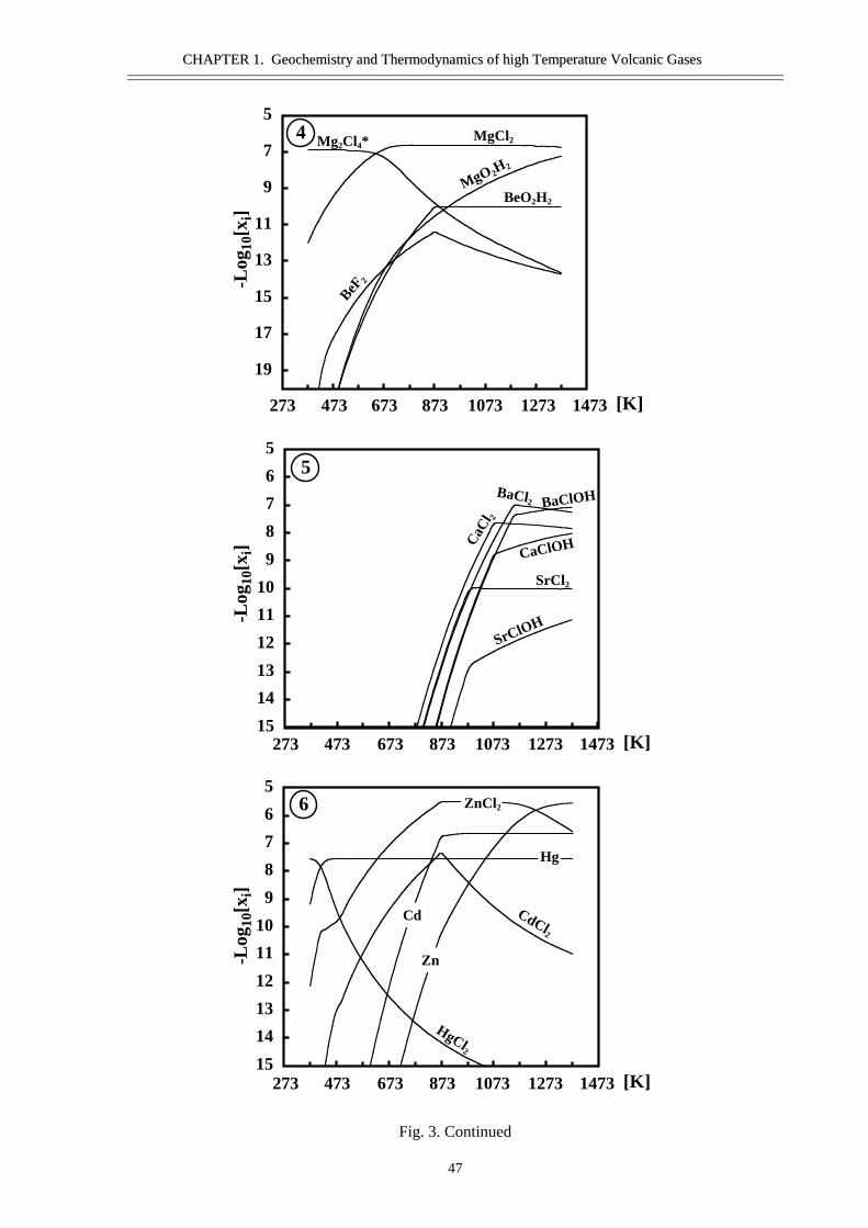
CCHHAAPPTTEERR 11.. GGeeoocchheemmiissttrryy aanndd TThheerrmmooddyynnaammiiccss ooff hhiigghh TTeemmppeerraattuurree VVoollccaanniicc GGaasseess————————————————————————————————————————————————————————————————————————————————————————————————————————————————
47
Fig. 3. Continued
BeF2
BeO2H2
MgCl2
MgO2H2
Mg2Cl4*
5
7
9
11
13
15
17
19
4
273 473 673 873 1073 1273 1473 [K]
-Log
10[x
i]
BaClOHBaCl2
SrCl2
SrClOH
CaClOHCaC
l 2
5
6
7
8
9
10
11
12
13
14
15
5
273 473 673 873 1073 1273 1473 [K]
-Log
10[x
i]
Hg
HgCl2
ZnCl2
Zn
Cd CdCl2
5
6
7
8
9
10
11
12
13
14
15
6
273 473 673 873 1073 1273 1473 [K]
-Log
10[x
i]
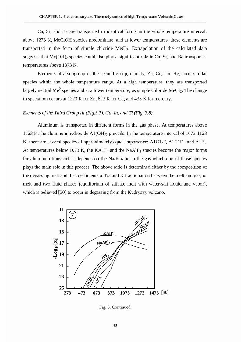
CCHHAAPPTTEERR 11.. GGeeoocchheemmiissttrryy aanndd TThheerrmmooddyynnaammiiccss ooff hhiigghh TTeemmppeerraattuurree VVoollccaanniicc GGaasseess————————————————————————————————————————————————————————————————————————————————————————————————————————————————
48
Ca, Sr, and Ba are transported in identical forms in the whole temperature interval:
above 1273 K, MeClOH species predominate, and at lower temperatures, these elements are
transported in the form of simple chloride MeCl2. Extrapolation of the calculated data
suggests that Me(OH)2 species could also play a significant role in Ca, Sr, and Ba transport at
temperatures above 1373 K.
Elements of a subgroup of the second group, namely, Zn, Cd, and Hg, form similar
species within the whole temperature range. At a high temperature, they are transported
largely neutral Me0 species and at a lower temperature, as simple chloride MeCI2. The change
in speciation occurs at 1223 K for Zn, 823 K for Cd, and 433 K for mercury.
Elements of the Third Group Al (Fig.3.7), Ga, In, and Tl (Fig. 3.8)
Aluminum is transported in different forms in the gas phase. At temperatures above
1123 K, the aluminum hydroxide A1(OH)3 prevails. In the temperature interval of 1073-1123
K, there are several species of approximately equal importance: A1C12F, A1C1F2, and A1F3.
At temperatures below 1073 K, the KA1F4 and the NaAlF4 species become the major forms
for aluminum transport. It depends on the Na/K ratio in the gas which one of those species
plays the main role in this process. The above ratio is determined either by the composition of
the degassing melt and the coefficients of Na and K fractionation between the melt and gas, or
melt and two fluid phases (equilibrium of silicate melt with water-salt liquid and vapor),
which is believed [30] to occur in degassing from the Kudryavy volcano.
Fig. 3. Continued
AlF3
AlCl2F
NaAlF4
KAlF4
AlO 3H3
11
13
15
17
19
21
23
25
AlC
l 3
AlC
lF2
7
273 473 673 873 1073 1273 1473 [K]
-Log
10[x
i]
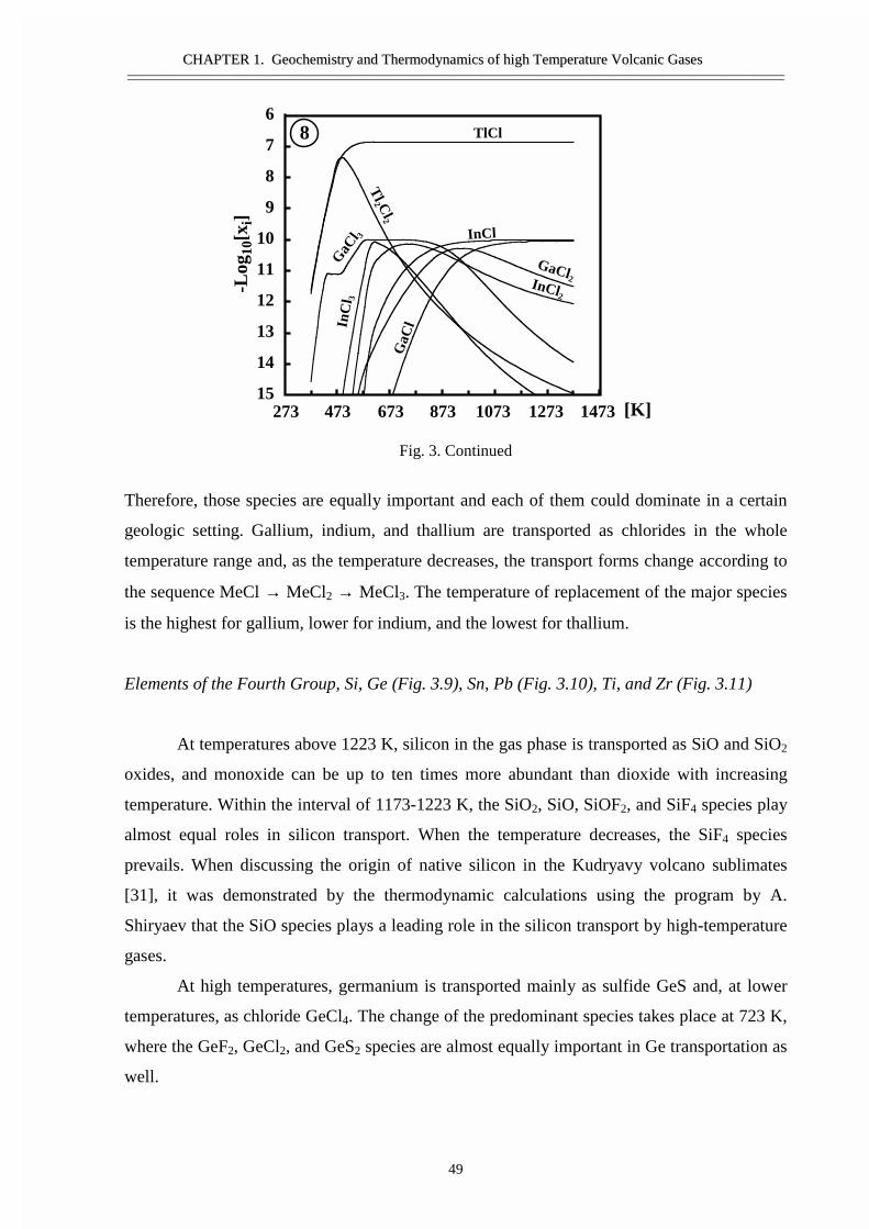
CCHHAAPPTTEERR 11.. GGeeoocchheemmiissttrryy aanndd TThheerrmmooddyynnaammiiccss ooff hhiigghh TTeemmppeerraattuurree VVoollccaanniicc GGaasseess————————————————————————————————————————————————————————————————————————————————————————————————————————————————
49
Fig. 3. Continued
Therefore, those species are equally important and each of them could dominate in a certain
geologic setting. Gallium, indium, and thallium are transported as chlorides in the whole
temperature range and, as the temperature decreases, the transport forms change according to
the sequence MeCl → MeCl2 → MeCl3. The temperature of replacement of the major species
is the highest for gallium, lower for indium, and the lowest for thallium.
Elements of the Fourth Group, Si, Ge (Fig. 3.9), Sn, Pb (Fig. 3.10), Ti, and Zr (Fig. 3.11)
At temperatures above 1223 K, silicon in the gas phase is transported as SiO and SiO2
oxides, and monoxide can be up to ten times more abundant than dioxide with increasing
temperature. Within the interval of 1173-1223 K, the SiO2, SiO, SiOF2, and SiF4 species play
almost equal roles in silicon transport. When the temperature decreases, the SiF4 species
prevails. When discussing the origin of native silicon in the Kudryavy volcano sublimates
[31], it was demonstrated by the thermodynamic calculations using the program by A.
Shiryaev that the SiO species plays a leading role in the silicon transport by high-temperature
gases.
At high temperatures, germanium is transported mainly as sulfide GeS and, at lower
temperatures, as chloride GeCl4. The change of the predominant species takes place at 723 K,
where the GeF2, GeCl2, and GeS2 species are almost equally important in Ge transportation as
well.
GaCl2
GaC
l
GaC
l 3
TlCl
Tl2 C
l2
InCl2
InCl
InC
l 3
6
7
8
9
10
11
12
13
14
15
8
273 473 673 873 1073 1273 1473 [K]
-Log
10[x
i]
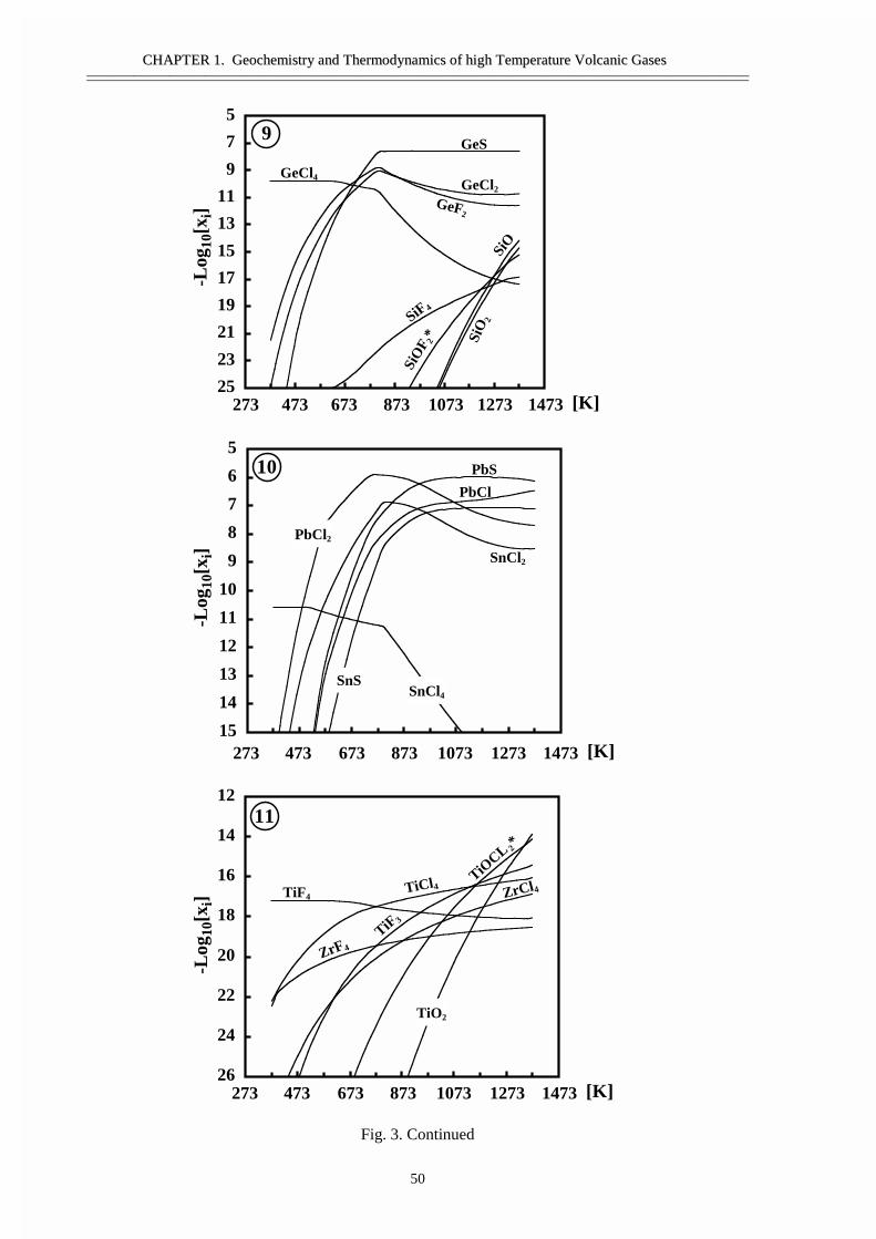
CCHHAAPPTTEERR 11.. GGeeoocchheemmiissttrryy aanndd TThheerrmmooddyynnaammiiccss ooff hhiigghh TTeemmppeerraattuurree VVoollccaanniicc GGaasseess————————————————————————————————————————————————————————————————————————————————————————————————————————————————
50
Fig. 3. Continued
SiO
SiO
2SiF 4
SiO
F 2*
GeCl2
GeCl4
GeF2
GeS
5
7
9
11
13
15
17
19
21
23
25
9
273 473 673 873 1073 1273 1473 [K]
-Log
10[x
i]
PbCl
PbCl2
PbS
SnCl2
SnCl4
SnS
5
6
7
8
9
10
11
12
13
14
15273 473 673 873 1073 1273 1473 [K]
10
-Log
10[x
i]
TiCl4TiF4
TiF 3
TiO2
TiOCL 2*
ZrCl4
ZrF4
12
14
16
18
20
22
24
26
11
273 473 673 873 1073 1273 1473 [K]
-Log
10[x
i]
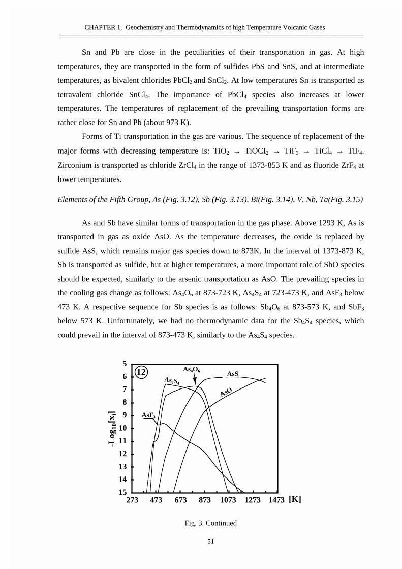
CCHHAAPPTTEERR 11.. GGeeoocchheemmiissttrryy aanndd TThheerrmmooddyynnaammiiccss ooff hhiigghh TTeemmppeerraattuurree VVoollccaanniicc GGaasseess————————————————————————————————————————————————————————————————————————————————————————————————————————————————
51
Sn and Pb are close in the peculiarities of their transportation in gas. At high
temperatures, they are transported in the form of sulfides PbS and SnS, and at intermediate
temperatures, as bivalent chlorides PbCl2 and SnCl2. At low temperatures Sn is transported as
tetravalent chloride SnCl4. The importance of PbCl4 species also increases at lower
temperatures. The temperatures of replacement of the prevailing transportation forms are
rather close for Sn and Pb (about 973 K).
Forms of Ti transportation in the gas are various. The sequence of replacement of the
major forms with decreasing temperature is: TiO2 → TiOCI2 → TiF3 → TiCl4 → TiF4.
Zirconium is transported as chloride ZrCl4 in the range of 1373-853 K and as fluoride ZrF4 at
lower temperatures.
Elements of the Fifth Group, As (Fig. 3.12), Sb (Fig. 3.13), Bi(Fig. 3.14), V, Nb, Ta(Fig. 3.15)
As and Sb have similar forms of transportation in the gas phase. Above 1293 K, As is
transported in gas as oxide AsO. As the temperature decreases, the oxide is replaced by
sulfide AsS, which remains major gas species down to 873K. In the interval of 1373-873 K,
Sb is transported as sulfide, but at higher temperatures, a more important role of SbO species
should be expected, similarly to the arsenic transportation as AsO. The prevailing species in
the cooling gas change as follows: As4O6 at 873-723 K, As4S4 at 723-473 K, and AsF3 below
473 K. A respective sequence for Sb species is as follows: Sb4O6 at 873-573 K, and SbF3
below 573 K. Unfortunately, we had no thermodynamic data for the Sb4S4 species, which
could prevail in the interval of 873-473 K, similarly to the As4S4 species.
Fig. 3. Continued
AsF3
AsO
As4O6 AsSAs4S4
5
6
7
8
9
10
11
12
13
14
15
12
273 473 673 873 1073 1273 1473 [K]
-Log
10[x
i]
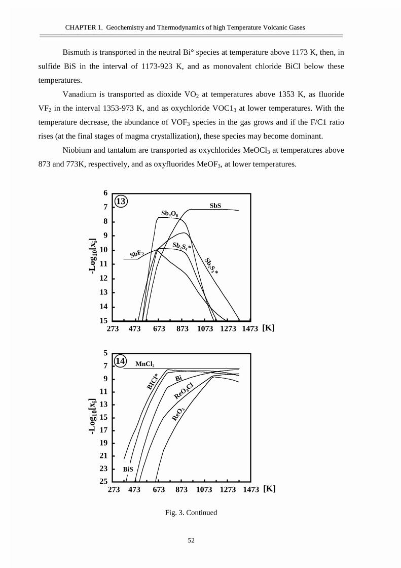
CCHHAAPPTTEERR 11.. GGeeoocchheemmiissttrryy aanndd TThheerrmmooddyynnaammiiccss ooff hhiigghh TTeemmppeerraattuurree VVoollccaanniicc GGaasseess————————————————————————————————————————————————————————————————————————————————————————————————————————————————
52
Bismuth is transported in the neutral Bi° species at temperature above 1173 K, then, in
sulfide BiS in the interval of 1173-923 K, and as monovalent chloride BiCl below these
temperatures.
Vanadium is transported as dioxide VO2 at temperatures above 1353 K, as fluoride
VF2 in the interval 1353-973 K, and as oxychloride VOC13 at lower temperatures. With the
temperature decrease, the abundance of VOF3 species in the gas grows and if the F/C1 ratio
rises (at the final stages of magma crystallization), these species may become dominant.
Niobium and tantalum are transported as oxychlorides MeOCl3 at temperatures above
873 and 773K, respectively, and as oxyfluorides MeOF3, at lower temperatures.
Fig. 3. Continued
Sb4O6
SbF3
SbS
Sb2 S
3 *
Sb2S4*
6
7
8
9
10
11
12
13
14
15
13
273 473 673 873 1073 1273 1473 [K]
-Log
10[x
i]
Bi
BiS
BIC
l*
MnCl2
ReO3C
l
ReO
3
5
7
9
11
13
15
17
19
21
23
25
14
273 473 673 873 1073 1273 1473 [K]
-Log
10[x
i]
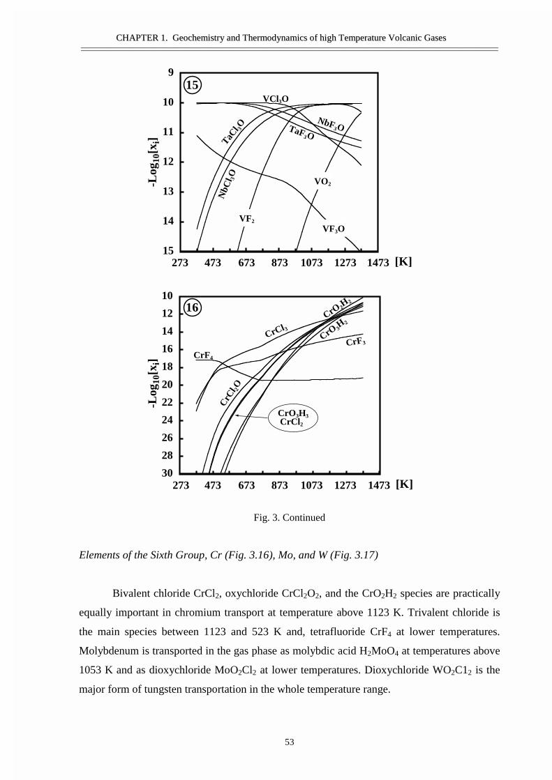
CCHHAAPPTTEERR 11.. GGeeoocchheemmiissttrryy aanndd TThheerrmmooddyynnaammiiccss ooff hhiigghh TTeemmppeerraattuurree VVoollccaanniicc GGaasseess————————————————————————————————————————————————————————————————————————————————————————————————————————————————
53
Fig. 3. Continued
Elements of the Sixth Group, Cr (Fig. 3.16), Mo, and W (Fig. 3.17)
Bivalent chloride CrCl2, oxychloride CrCl2O2, and the CrO2H2 species are practically
equally important in chromium transport at temperature above 1123 K. Trivalent chloride is
the main species between 1123 and 523 K and, tetrafluoride CrF4 at lower temperatures.
Molybdenum is transported in the gas phase as molybdic acid H2MoO4 at temperatures above
1053 K and as dioxychloride MoO2Cl2 at lower temperatures. Dioxychloride WO2C12 is the
major form of tungsten transportation in the whole temperature range.
VCl3O
VF3O
VO2
VF2N
bCl 3O
NbF3O
TaCl 3O TaF
3O
9
10
11
12
13
14
15
15
273 473 673 873 1073 1273 1473 [K]
-Log
10[x
i]
CrCl3
CrCl2
CrF3
CrC
l 2O
CrO3H3
CrF4
CrO3H
2CrO2H
210
12
14
16
18
20
22
24
26
28
30
16
273 473 673 873 1073 1273 1473 [K]
-Log
10[x
i]
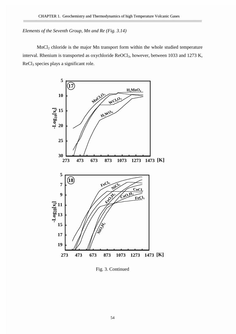
CCHHAAPPTTEERR 11.. GGeeoocchheemmiissttrryy aanndd TThheerrmmooddyynnaammiiccss ooff hhiigghh TTeemmppeerraattuurree VVoollccaanniicc GGaasseess————————————————————————————————————————————————————————————————————————————————————————————————————————————————
54
Elements of the Seventh Group, Mn and Re (Fig. 3.14)
MnCl2 chloride is the major Mn transport form within the whole studied temperature
interval. Rhenium is transported as oxychloride ReOCl3, however, between 1033 and 1273 K,
ReCl3 species plays a significant role.
Fig. 3. Continued
WCl2O2
H2WO4
H2MoO4
MoCl 2O2
5
10
15
20
25
30
17
273 473 673 873 1073 1273 1473 [K]
-Log
10[x
i]
FeCl3
FeCl2
FeO2H
2
CoCl2
CoO2H2
NiCl 2
NiO
2H2
5
7
9
11
13
15
17
19
18
273 473 673 873 1073 1273 1473 [K]
-Log
10[x
i]
CCHHAAPPTTEERR 11.. GGeeoocchheemmiissttrryy aanndd TThheerrmmooddyynnaammiiccss ooff hhiigghh TTeemmppeerraattuurree VVoollccaanniicc GGaasseess————————————————————————————————————————————————————————————————————————————————————————————————————————————————
55
Elements of the Eighth Group, Subgroup of Iron, Fe, Co, and Ni (Fig. 3.18)
As we expected, the elements of the iron subgroup have similar transportation forms.
These elements are transported as bivalent chlorides MeCl2 in the whole temperature range.
The role of hydroxides Me(OH)2 is higher at temperatures above 1273 K, while at lower
temperatures, a more oxidized trivalent iron transported as FeCl3 becomes more important.
GENERAL REGULARITIES OF GAS TRANSPORT
The calculation demonstrated that behaviour of all the elements is governed by
common regularities, the knowledge of which enables to predict the element species that have
not been included into the calculation due to the lack of thermodynamic data.
All of the elements tend to form simpler species (i.e., with decreasing number of
atoms in a molecule) at higher temperatures. Sometimes, this dependence is not obvious, and
the same major species prevails over the whole temperature interval; then the regularity is true
for the second important species. For elements of constant valence, this tendency is
manifested in the gradual polymerization of molecules with decreasing temperature. Alkali
metals which are transported at high temperatures as a simple chloride MeCl present a typical
example of such behaviour. With a temperature decrease they polymerize to dichloride
(MeCl)2. Similar properties were exhibited by Mg, Cu, and Tl. Elements of variable valence
form more complex molecules by increasing the valence of their cations at lower
temperatures. This is exemplified by Zn, Cd and Hg showing replacement of neutral Me0
species by MeCl2 chloride with the temperature growth. The changes in Ga and In species
correspond to the sequence of MeCl → MeCl2 → MeCl3. MeCl2 is substituted by MeCl4 for
Sn and Ge, while SiO is replaced by SiO2. According to the calculation, Al, Cr, W, Mo, and
Re are transported as complex species at the highest temperatures of the studied interval.
Consequently, we may expect the occurrence of simpler molecules at even higher
temperatures.
The analysis of element speciation reveals that, at the lower temperatures, most of the
elements are transported as halogenides. At high temperatures, the predominant forms are
sulfides (SnCl4 → SnS; PbCl2 → PbS; AsF3 → AsS; SbF3 → SbS), oxides (SiF4 → SiO2 →
SiO; TiF4 → ... → TiO2), hydroxides (FeCl2 → Fe(OH)2; CrF4 → ... → Cr(OH)2), and
monatomic species (ZnCl2 → Zn; CdCl2 → Cd; BiCl → ... → Bi). Similar regularities were
discovered in the mineral equilibria [32]. Studies of exchange reactions showed an increase in
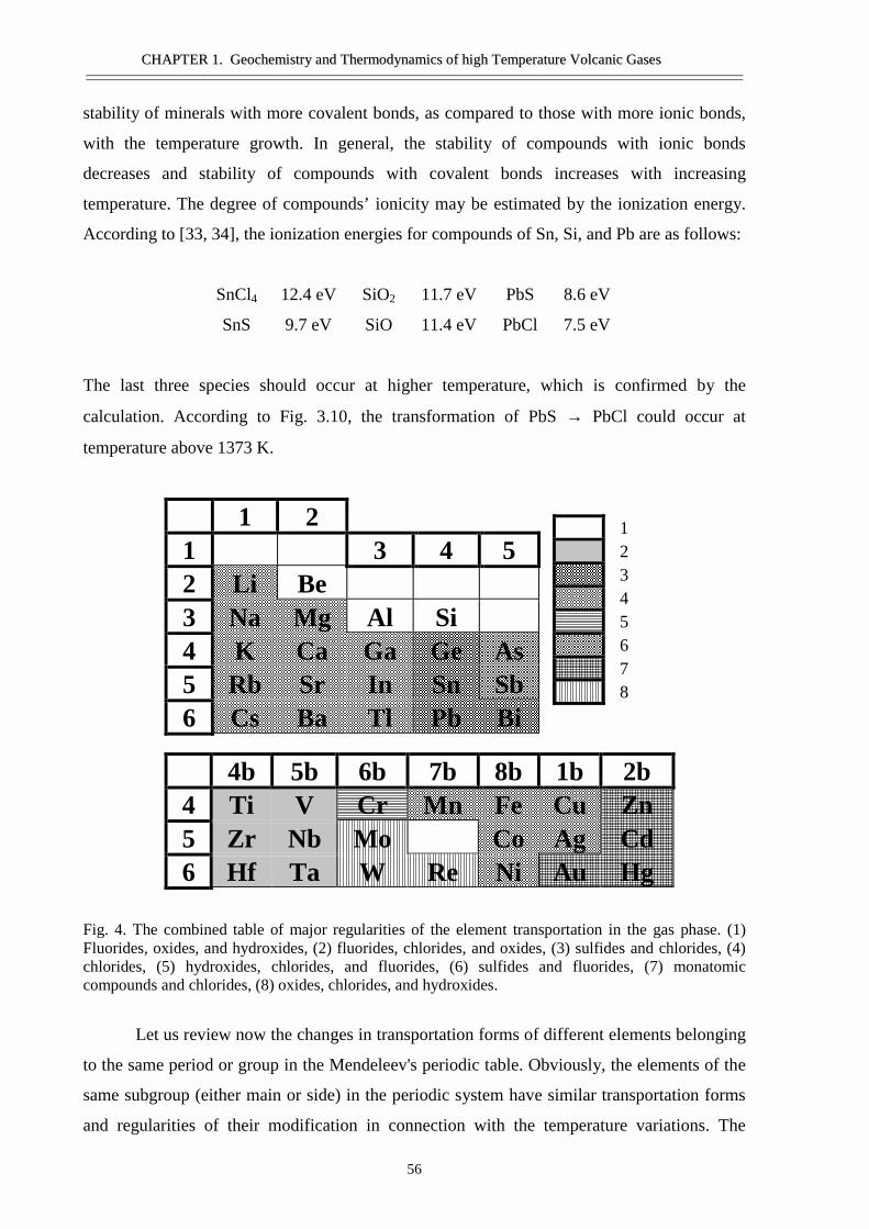
CCHHAAPPTTEERR 11.. GGeeoocchheemmiissttrryy aanndd TThheerrmmooddyynnaammiiccss ooff hhiigghh TTeemmppeerraattuurree VVoollccaanniicc GGaasseess————————————————————————————————————————————————————————————————————————————————————————————————————————————————
56
stability of minerals with more covalent bonds, as compared to those with more ionic bonds,
with the temperature growth. In general, the stability of compounds with ionic bonds
decreases and stability of compounds with covalent bonds increases with increasing
temperature. The degree of compounds’ ionicity may be estimated by the ionization energy.
According to [33, 34], the ionization energies for compounds of Sn, Si, and Pb are as follows:
SnCl4 12.4 eV SiO2 11.7 eV PbS 8.6 eV
SnS 9.7 eV SiO 11.4 eV PbCl 7.5 eV
The last three species should occur at higher temperature, which is confirmed by the
calculation. According to Fig. 3.10, the transformation of PbS → PbCl could occur at
temperature above 1373 K.
1 21 3 4 52 Li Be3 Na Mg Al Si4 K Ca Ga Ge As5 Rb Sr In Sn Sb6 Cs Ba Tl Pb Bi
12345678
4b 5b 6b 7b 8b 1b 2b4 Ti V Cr Mn Fe Cu Zn5 Zr Nb Mo Co Ag Cd6 Hf Ta W Re Ni Au Hg
Fig. 4. The combined table of major regularities of the element transportation in the gas phase. (1)Fluorides, oxides, and hydroxides, (2) fluorides, chlorides, and oxides, (3) sulfides and chlorides, (4)chlorides, (5) hydroxides, chlorides, and fluorides, (6) sulfides and fluorides, (7) monatomiccompounds and chlorides, (8) oxides, chlorides, and hydroxides.
Let us review now the changes in transportation forms of different elements belonging
to the same period or group in the Mendeleev's periodic table. Obviously, the elements of the
same subgroup (either main or side) in the periodic system have similar transportation forms
and regularities of their modification in connection with the temperature variations. The
CCHHAAPPTTEERR 11.. GGeeoocchheemmiissttrryy aanndd TThheerrmmooddyynnaammiiccss ooff hhiigghh TTeemmppeerraattuurree VVoollccaanniicc GGaasseess————————————————————————————————————————————————————————————————————————————————————————————————————————————————
57
heavier elements change their major (similar) transportation forms at lower temperatures. For
example, for zinc, cadmium, and mercury the Me0 → MeCl2 transformation occurs at
respective temperatures of 1273, 873, and 453 K. The transformation of gallium and indium
species occurs in the sequence MeCl → MeCl2 → MeCl3 in the intervals of 1023-873 K and
793-653 K, respectively. A similar dependence is also typical of some elements from the
other groups: Pb-Sn-Ge, Ti-Zr, and Sb-As. Such regularities are less pronounced for elements
belonging to different groups of the same period.
Considering the relationships between the element species and position of these
elements in the long period version of the Mendeleev's periodic table (Fig. 4), we can draw
the following conclusions. In the major subgroup, elements located in the top right-hand part
of the table (Be, Al, and Si) are transported in the form of fluorides and oxides. Elements in
the right part of the table (As, Sb) are transported in the form of sulfides and oxides. The
bottom left-hand corner is occupied by elements with chloride transportation forms (Li, Na,
K, Rb, Cs, Mg, Ca, Sr, Ba, Ga, In, and Tl). Elements of intermediate location in the table (Ge,
Sn, Pb, and Bi) have both sulfide and chloride transportation forms. Elements of the side
group may be described as follows. The top left-hand part is occupied by elements with the
fluoride and chloride transportation forms (Ti, Zr, and V). When moving to the right, these
forms are replaced by oxyfluorides and oxychlorides (Nb, Ta, Cr, Mo, W, and Re), then
chlorides (Fe, Co, Ni, Cu, and Zn) and, finally, Hg is transported as a neutral species in almost
the whole range of temperatures examined.
Therefore, the transportation forms for all the elements are in close relation with their
position in the Mendeleev's periodic table. The behaviour of the volatile forms of elements,
similarly to the behaviour of the elements themselves, is controlled by general regularities, the
knowledge of which enables to forecast the dependence of transportation forms on
temperature for elements not included into the calculation.
For example, considering the position of silver and gold in the periodic table, we may
expect that their properties, on the one hand, must be close to those of copper and, on the
other hand, to the properties of zinc, cadmium, and mercury. We may suppose that gold and
silver will be transported as neutral species and chlorides of a MeCl type. A calculation of the
element transportation forms in the gases from Mount Saint Helens volcano [13] revealed that
silver is transported as AgCl, which agrees with our assumption. On the other hand, according
to the calculation, sulfide AuS was the major transportation form for gold [13]. This could be
resulted from the absence of gold chloride species in the applied database [13]. However, this
species may play the major role in Au transportation. This example demonstrates that the
CCHHAAPPTTEERR 11.. GGeeoocchheemmiissttrryy aanndd TThheerrmmooddyynnaammiiccss ooff hhiigghh TTeemmppeerraattuurree VVoollccaanniicc GGaasseess————————————————————————————————————————————————————————————————————————————————————————————————————————————————
58
completeness and reliability of thermodynamic data involved in calculation are the most
important prerequisites for an adequate approximation to natural processes with calculations
of this kind.
CONCLUSIONS
(1) Based on the data on the composition of gases and condensates, a thermodynamic
modelling of a high-temperature cooling gas from the Kudryavy volcano has been performed.
Transportation and deposition forms have been calculated for most ore and rock-forming
elements.
(2) The calculated mineral stability and the temperatures of deposition of most minerals
correspond well to the data on their crystallization from volcanic gases. Consequently, the
model takes into account rather completely and correctly those forms of the element
transportation and deposition, which play the leading role in their transportation by high-
temperature fumarolic gases.
(3) The alkali and alkali earth metals, Ga, In, Tl, Fe, Co, Ni, Cu, and Zn are mainly
transported as chlorides in the gas phase. Ge, Sn, Pb, and Bi occur as sulfide and chloride
species, at intermediate and low temperatures. Be, Al, and Si are transported as fluorides and
oxides, while As and Sb, as sulfides and oxides. More complex, oxyfluoride and oxychloride
transportation forms are dominant for Ti, Zr, V, Mo, W, and Re. Cd at a high temperature and
Hg in the whole temperature range are transported as neutral species.
(4) Forms of transportation of all elements in gas are closely related to the position of
these elements in the Mendeleev's periodic table. The behaviour of the volatile element forms,
like the behaviour of the elements themselves, is controlled by the following general
regularities: (a) all the elements follow a tendency of simplifying the major transportation
forms, i.e., decreasing the number of atoms in the molecule at higher temperatures. For
elements of a constant valence, this tendency is manifested in gradual polymerization of their
molecules as the temperature decreases; (b) as the temperature rises, the stability of
compounds with ionic bonds decreases, but that of compounds with covalence bonds
increases; (c) similar species transformations takes place at lower temperatures for heavier
elements.
ACKNOWLEDGEMENTS
We are grateful to D. V. Grichuk, staff member of the Geochemistry Department of
CCHHAAPPTTEERR 11.. GGeeoocchheemmiissttrryy aanndd TThheerrmmooddyynnaammiiccss ooff hhiigghh TTeemmppeerraattuurree VVoollccaanniicc GGaasseess————————————————————————————————————————————————————————————————————————————————————————————————————————————————
59
the Moscow State University for making available the GBGAS software as well as for his
help in the interpretation of the results and for valuable remarks when preparing this paper.
REFERENCES
1. Symonds, R.B., Rose, W.I., Gregg, J., et al, Volcanic Gas Studies: Methods, Results and
Applications, in Review in Mineralogy, vol. 30: Volatiles in Magmas, Carroll, M.R. and
Holloway, J.R., Eds., 1994, pp. 1-66.
2. Giggenbach, W.F., Chemical Composition of Volcanic Gases, in Monitoring and
Mitigation of Volcano Hazards, Scarpa, R. and Tilling, R.I., Eds. Berlin: Springer, 1996,
pp. 221-256.
3. Stoiber, R.E. and Rose, W.I., The Geochemistry of Central American Volcanic Gas
Condensates, Geol. Soc. Am. Bull., 1970, vol. 81, pp. 2891-2912.
4. Gemmell, J.B., Geochemistry of Metallic Trace Elements in Fumarolic Condensates from
Nicaraguan and Costa Rican Volcanoes, J. Volcanol. Geotherm. Res., 1987, vol. 33, pp.
161-181.
5. Symonds, R.B., Rose, W.I., Reed, M.H., et al, Volatilization, Transport and Sublimation
of Metallic and Non-Metallic Elements in High Temperature Gases at Merapi Volcano,
Indonesia, Geochim. Cosmochim. Acta, 1987, vol. 51, pp. 2083-2101.
6. Symonds, R.B., Rose, W.I., Gerlach, T.M., et al., Evaluation of Gases, Condensates, and
SO2 Emission From Augustine Volcano, Alaska: the Degassing of a Cl-Rich Volcanic
System, Bull. Volcanol., 1990, vol. 52, pp. 355-374.
7. Quisefit, J.P., Toutain, J.P., Bergametti, G., et al., Evolution versus Cooling Gaseous
Volcanic Emissions from Momotombo Volcano, Nicaragua: Thermochemical Model and
Observations, Geochim. Cosmochim. Acta, 1989, vol. 53, pp. 2591-2608.
8. Symonds, R.B., Scanning Electron Microscope Observations of Sublimates from Merapi
Volcano, Indonesia, Ceochem. J., 1993, vol. 26, pp. 337-350.
9. Le Guern, F. and Bernard, A., A New Method for Sampling and Analyzing Volcanic
Sublimates - Application to Merapi Volcano, Java, J. Volcanol. Geotherm. Res., 1982,
vol. 12, pp. 133-146.
10. Bernard, A. and Le Guern, F, Condensation of Volatile Elements in High-Temperature
Gases of Mount St. Helens, J. Volcanol. Geothefrn. Res., 1986, vol. 28, pp. 91-105.
11. Le Guern, F, Cheynet, B., and Faivre-Pierret, R.X., Characterization and Modeling of the
Complete Volcanic Gas Phase, Geochem. J., 1993, vol. 27, pp. 323-336.
12. Symonds, R.B., Reed, M.H., and Rose, W.I., Origin, Speciation, and Fluxes of Trace-
CCHHAAPPTTEERR 11.. GGeeoocchheemmiissttrryy aanndd TThheerrmmooddyynnaammiiccss ooff hhiigghh TTeemmppeerraattuurree VVoollccaanniicc GGaasseess————————————————————————————————————————————————————————————————————————————————————————————————————————————————
60
Element Gases at Augustine Volcano, Alaska: Insights into Magma Degassing and
Fumarolic Processes, Geochim. Cosmochim. Acta, 1992, vol. 56, pp. 633-657.
13. Symonds, R.B. and Reed, M.H., Calculation of Multicomponent Chemical Equilibria in
Gas-Solid-Liquid Systems: Calculation Methods, Thermochemical Data, and Applications
to Studies of High-Temperature Volcanic Gases with Examples from Mount St. Helens,
Am. J. Sci, 1993, vol. 293, pp. 758-864.
14. Taran, Yu.A., Hedenquist, J.F, Korzhinskii, M.A., et al., Geochemistry of Magmatic
Gases From Kudryavy Volcano, Iturup, Kuril Islands, Geochim. Cosmochim. Acta, 1995,
vol. 59, pp. 1749-1761.
15. Gorshkov, G.S., Vulkanizm Kuril'skoi ostrovnoi dugi (Volcanism of the Kurile Island
Arc), Moscow: Nauka, 1967.
16. Ostapenko, V.F., Petrology of Calderas of the Kurile Islands: Medvezhii and Zavaritskii
Calderas, in Geologiya igeofizika okeanov (Geology and Geophysics of the Oceans),
Mater. Sakhalin. Issled. Inst., 1970, vol. 25, pp. 159-176.
17. Pawley, A.R. and Holloway, J.R., Water Sources for Subduction Zone Volcanism: New
Experimental Constrains, Sciences, 1993, vol. 260, pp. 664-667.
18. Tkachenko, S.I., High-Temperature Fumarolic Gases, Condensates, and Sublimates of the
Kudryavy Volcano, Iturup Island, Kurile Islands, Cand. Sc. (Geol.-Mineral.) Dissertation,
Chernogolovka: Inst. Exp. Miner., 1996.
19. Melody geokhimicheskogo modelirovaniya i prognozirovaniya v gidrogeologii (Methods
of Geochemical Modeling and Prediction in Hydrogeology), Moscow: Nedra, 1988.
20. Termodinamicheskie svoistva individual'nykh veshchestv (Thermodynamic Properties of
Individual Compounds), Moscow: Nauka, 1978-1982, vols. 1-4.
21. Baryshnikov, N.V. and Zelikman, D.T., Thermodynamic Properties of Re Chlorides and
Oxides, Izv. tyssh. Uchebn. Zaved., Tsvetn. Metal, 1962, no. 6, pp. 98-110.
22. Robie, R.A., Hemingway, B.S., and Fisher, J.R., Thermodynamic Properties of Minerals
and Related Substances at 298.15 K and 1 bar Pressure and at Higher Temperatures, Bull.
U.S. Dep. Interior. Geol. Surv. Washington: U.S. Gov. Print. Off 1978, vol. 1452.
23. Tkachenko, S.I., Porter, R.R, Korzhinskii, M.A., et al., Study of Processes of Ore and
Mineral Formation from the High-Temperature Fumarolic Gases on the Kudryavy
Volcano, Iturup Island, Kurile Islands, Geokhimiya, 1999, vol. 37, no. 4, pp. 410-422.
24. Vinogradov, A.P., Average Abundances of Chemical Elements in the Main Types of
Igneous Rocks, Geokhimiya, 1962, no. 7, pp. 555-571.
25. Toutain, J.P., Person, A., Cheminee, J.L., et al, Mineralogie des sublimes du Volcan Poas
CCHHAAPPTTEERR 11.. GGeeoocchheemmiissttrryy aanndd TThheerrmmooddyynnaammiiccss ooff hhiigghh TTeemmppeerraattuurree VVoollccaanniicc GGaasseess————————————————————————————————————————————————————————————————————————————————————————————————————————————————
61
(Costa Rica), C. R. Acad. ScL, Set: II: ScL Terre Planetes, 1985, vol. 15, pp. 769-772.
26. Rosen, E., Osadchii, Eu., and Tkachenko, S., Oxygen Fugacity Directly Measured in
Fumaroles of the Volcano Kudrjaviy (Kuril Isles), Chem. Erde, 1993, vol. 53, pp. 219-
227.
27. Osadchii, E.G., Lunin, S.E., Korzhinskii, M.A., et al, Measurement of fO2 and fS2 by
Electrochemical Sensors in High-Temperature Fumaroles of Active Volcanoes,
Geokhimiya, 1997, no. 1, pp. 74-81.
28. Giggenbach, W.F., Redox Processes Governing the Chemistry of Fumarolic Gas
Discharges from White Islands, New Zealand, Appl Geochem., 1987, vol. 2, pp. 143-161.
29. Murata, K.J., Occurrence of CuCl Emission in Volcanic Flames, am. J. ScL, I960, vol.
258, pp. 769-772.
30. Shmulovich, K.I., Formation of Salt Melts during Magmalic Degassing in an Open
System: Evidence from the Kudryavyi Volcano, Iturup Island, the Kurils, Doki Ross.
Akad. Nauk, 1999, vol. 365, no. 3, pp. 361-365.
31. Shmulovich, K.I., Vakulenko, A.G., and Shiryaev, A.A., Formation of Native Silicon in
Sublimates of the Kudryavyi Volcano, Iturup Island, Kurils Islands, Dokl Ross. Akad.
Nauk, 1997, vol. 354, no. 6, pp. 800-803.
32. Purchuk, L.L. and Ryabchikov, I.D., Fazovoe sootvetstvie v mineral'nykh sistemakh
(Phase Correspondence in Mineral Systems), Moscow: Nedra, 1976.
33. Fizicheskie velichiny: Spravochnik (Physical Values: A Handbook), Grigor'ev, I.S. and
Meilikhov, E.Z., Eds., Moscow: Energoatomizdat, 1991.
34. Energii razryva khimicheskikh svyazei. Potentsialy ionizatsii i srodstvo k elektronn
(Energy of Disruption of Chemical Bonds. lonization Potentials and Electron Affinity),
Kondrafeva, V.N., Ed., Moscow: Nauka, 1974.

Perturbation Theory Based Equation of State for Polar Molecular Fluids:
I. Pure Fluids
CHAPTER II. An Equation of State for Complex Mixtures of non-Electrolytes————————————————————————————————————————————————————————
63
ABSTRACT
Based on the thermodynamic perturbation theory an equation of state (EOS) for
molecular fluids has been formulated which can be used for many fluid species in geological
systems. The EOS takes into account four substance specific parameters, which are the
molecular dipole moment, the molar polarizability and the two parameters of the Lennard-
Jones potential. For the most important fluids these parameters are available from
experimental measurements. In lack of direct experimental determinations, as a first
approximation, for a pure fluid these parameters can also be evaluated using the critical
temperature and the critical density in addition to the dipole moment for polar molecules with
reasonable accuracy. The EOS has the appropriate asymptotic behaviour at high pressures and
temperatures. Currently parameters for 98 inorganic and organic compounds are available. In
this article the EOS for pure fluids is presented. In a further communication the EOS is
extended to fluid mixtures (Churakov and Gottschalk, submitted to GCA).
CHAPTER II. An Equation of State for Complex Mixtures of non-Electrolytes————————————————————————————————————————————————————————
64
Table 1. Notation and symbols
α, α* molecular polarizability, reduced polarizabilityε, σ parameters of Lennard-Jones potentialϕ fugacity coefficientµ, µ* dipole moment, reduced dipole moment
ρ, ρ* density, reduced density
ρc, ρc* critical density, reduced critical density
A Helmholtz free energyJ, K integrals over the pair and triple distribution functionsNA Avogadro´s numberP pressurePc, Pc
* critical pressure, reduced critical pressure
T temperature,Tc, Tc
* critical temperature, reduced critical temperature
U internal energyZ compressibility
r distancef fugacityu potential energy
1. INTRODUCTION
Fluids are important for many geological and petrological processes in the Earth's
crust and mantle. For the evaluation of such processes the thermodynamic properties of these
fluids are needed. The required free energies, i.e. fugacities, of the fluid components at high
pressure and temperature are usually derived using equations of state (EOS). Several
approaches are currently used to derive equations of state. For geological purposes these are
sophisticated modifications to the van der Waals equation (e.g. Holloway, 1976; Jacobs and
Kerrick, 1981; Kerrick and Jacobs, 1981; Halbach and Chatterjee 1982; Holland and Powell,
1991; Grevel and Chatterjee, 1992; Anderko and Pitzer, 1993a, 1993b; Duan et al., 1995b),
virial equations of state (e.g. Saxena and Fei, 1987, 1988; Duan et al., 1992a, 1992b; Sterner
and Pitzer, 1994) and other equations based on the thermodynamic perturbation theory (e.g.
Shmulovich at al., 1982; Ree, 1984). In all these EOS the required coefficients are determined
primarily using experimental results (e.g. PVT-data, phase equilibria). As an alternative to
experimental results, fluid properties can be derived by computer simulations considering
molecular interaction potentials (e.g. Brodholt and Wood, 1990, 1993a, 1993b; Belonoshko

CHAPTER II. An Equation of State for Complex Mixtures of non-Electrolytes————————————————————————————————————————————————————————
65
and Saxena 1991a, 1991b, 1992; Duan et al., 1992c, 1995a, 1996, 2000; Kalinichev and
Heinzinger, 1995; Destrigneville et al., 1996).
All types of EOS mentioned are based on physical models and require various
coefficients. If the physical description used by an EOS is perfect all required coefficients will
have an exact physical meaning. Molecular interactions are manifold, however. Types of
interactions involve repulsion due to a finite size of the molecules, attraction between
permanent and induced dipoles, quadrupole and higher multipoles, and in addition dispersion
forces. In the case of charged molecules coulomb interaction forces must be taken into
account. Therefore any EOS uses simplifications by grouping sets of similar interactions into
specific terms and therefore the precise physical significance of the required coefficients fades
or is even lost. Fitting experimental data to an EOS reveals then in many cases coefficients
with complicated functional dependencies with respect to temperature and either pressure or
volume and are therefore often described using empirical functions such as polynomials. The
use of arbitrary functions with questionable or no physical meaning transforms these EOS
into empirical equations. Such empirical approaches generally offer relatively simple explicit
expressions which are very attractive from a computational point of view. However, the
determination of the coefficients of such EOS requires a large experimental database over the
entire P-T range for which the equation is intended to be used. Generally, it can not be safely
extrapolated. Furthermore, because of the applied simplifications, these EOS are often unable
to reproduce available experimental data with the required accuracy. The accuracy can be
improved by introducing additional totally empirical parameters, which will dramatically
degrade the reliability of any extrapolation. All EOS based on the van der Walls equation of
state are therefore more or less empirical.
An alternative to EOS derived from the van der Walls equation are equations based on
the perturbation theory. In general an EOS based on the perturbation theory is an equation
which connects the macroscopic properties of a fluid (volume, temperature, pressure) to the
parameters of intermolecular interaction. The general idea of the thermodynamic perturbation
theory can be described as follows (e.g. Gray and Gubbins, 1984).
The potential of intermolecular interaction u of a real fluid can be always expressed as
the sum of a model dependent interaction potential u0 (the reference potential) and the
residual potential u1 which considers the differences of an interaction in the real fluid and the
reference model. For any given u and u0, a parametrical potential depending on a perturbation
parameter λ can be formulated:
CHAPTER II. An Equation of State for Complex Mixtures of non-Electrolytes————————————————————————————————————————————————————————
66
V u u u u u( ) ( )λ λ λ= + − = +0 0 0 1 (1)
It follows that V(0) = u0 and V(1) = u. The configurational part of the Helmholtz free energy
A , i.e. the part of energy depending only on intermolecular or interatomic interaction forces,
for a thermodynamic system of N molecules can be expressed at constant T and V by eq. (2)
using the configurational integral z (eq. 3) which is the integral over all possible
configurations Γ of N molecules.
A RT z= − ln( ) (2)
zu
RTd= −∫ exp(
( ))
Γ Γ (3)
If in eq. (3) u will be substituted by the parameterized potential V(λ) (eq. 1), the Helmholtz
free energy A can be expressed as a power series of the perturbation parameter λ:
A AA A A
( )! !
...λ λλ
λλ
λλλ
λ λ λ
= + ∂∂
+ ∂
∂
+ ∂∂
+== = =
00
2 2
20
3 3
302 3
(4)
As a first approximation the second and higher order terms can be neglected. Noting that
u = V(λ=1), the first order approximation of the Helmholtz free energy for the system of N
molecules interacting with the potential u can be obtained as
A RT z z uu
RTd A A= − + − = +− ∫ln( ) exp( )0 0
11
00 1Γ (5)
zu
RTd0
0= −∫ exp( ) Γ (6)
Thus the energy A of a thermodynamic system with the potential u can be expressed as the
sum of the energy A0 of the reference system of molecules with the interaction potential u0
and the perturbation term A1. The approximation requires, however, that u1 is small and the
reference potential u0 is therefore close to the interaction potential in the real fluid. The
accuracy can be improved, if the higher order terms in eq. (4) will be considered.
Strict application of the perturbation theory requires that the integral representing the
term A1 in eq. (5) is solved. Some approaches (e.g. Anderko and Pitzer, 1993a, 1993b; Duan
CHAPTER II. An Equation of State for Complex Mixtures of non-Electrolytes————————————————————————————————————————————————————————
67
et al, 1995b) avoid this complication, by combining A0 for the reference system with an
empirical approximation for the perturbation term A1 without assumptions on the character of
the intermolecular interaction in the fluid. But an EOS formulated in such a way becomes
again empirical in character and the capability of extrapolation will be lost. One aim of this
study is to formulate an EOS which is suitable for extrapolations to high pressures and
temperatures. Therefore we insist on using a type of equation like eq. (5) for the formulation
of the EOS which is based on the strict physical model of intermolecular interaction. Because
it is an approximation we realize that this model may also deviate from the interaction of real
molecules under extrapolation which will lead to deviations of the calculated thermodynamic
properties. However these deviations are expected to be at least small, because the model is
based on physical assumptions.
Most available experimental data are for pure fluids. PVT-data for fluid mixtures are
rare and extraction of fluid properties of fluid mixtures requires interpolation. As a first
approximation the van der Waals one-fluid theory is commonly used and parameters of pure
fluids are combined algebraically. Their application requires, however, that for each involved
fluid component the EOS is exactly of the same type. Most published EOS are for one or only
few fluid components and the EOS from different communications are rarely of the same
type. Therefore these EOS can not be used to derive fluid properties in complex mixtures
which have not been studied experimentally. In addition the mixing rules generally used are
not strictly in accordance with statistical mechanics. Dohrn and Prausnitz (1990) showed in a
systematic study of different fluid mixtures that van der Waals mixing rules may predict an
unrealistic physical behaviour such as increasing volume with pressure. Nevertheless one of
the aims of this study was to formulate an EOS which is suitable for as many components as
possible, so that this EOS can be applied in a further step to complex fluid mixtures
(Churakov and Gottschalk, submitted to GCA).
In the following an EOS is formulated using the perturbation theory with the Lennard-
Jones potential as the reference system. The EOS is applied to 98 pure inorganic and organic
fluid components and has the following attractive features. It needs a minimum number of
fitting parameters and its asymptotic behaviour at high pressure and temperature is physically
correct. As far as the form of the EOS is identical for all 98 considered fluid components the
EOS can be easily extended to the complex fluid mixtures using mixing rules. Fluid mixtures
will be covered in a second communication (Churakov and Gottschalk, submitted).
CHAPTER II. An Equation of State for Complex Mixtures of non-Electrolytes————————————————————————————————————————————————————————
68
2. THERMODYNAMIC MODEL
In this section only the principal aspects of the proposed EOS are discussed. Details
for the computational implementation can be found in the Appendix II.1.
The main contribution to the potential interaction energy between two polar molecules
i and j (eq. 7) is given by the sum of the Lennard-Jones potential (eq. 8), the potential due to
dipole-dipole (eq. 9) and to dipole-induced dipole interaction (eq. 10) which is the generalized
Stockmayer potential (e.g. Hirschfelder et al., 1964).
u u u uij ijLJ
ijdip dip
ijind dip= + +− − (7)
ur rij
LJij
ij
ij
ij
ij
=
−
4εσ σ
12 6
(8)
3
)cos(sinsincoscos2
ij
jijijiji
dipdipij
ru
φφθθθθµµ
−+−=− (9)
urij
ind dip i j j i
ij
− = −+α µ α µ2 2
6(10)
Here r is the distance between the centres of two molecules, θ and φ are the angles defining
the relative orientation of its dipoles, σ and ε are the specific parameters of interaction of the
Lennard-Jones potential, α is the average polarizability of a molecule and µ its dipole
moment. Although, eqs. (7)-(10) also hold for interactions between different molecules, in
this part of the communication only interactions between molecules of the same type are
considered. In the case of interaction of two non-polar molecules the potentials uijdip dip− and
uijind dip− are both zero and therefore only uij
LJ remains.
These potentials (eqs. 7-10) can be used to derive an EOS for molecular fluids based
on perturbation theory (e.g. Gray and Gubbins, 1984). Because the thermodynamic properties
of the Lennard-Jones potential are well known, it is convenient to take the Lennard-Jones
potential as the reference system and consider all contributions from other interactions
(dipole-dipole, dipole-induced dipole) as perturbations, i.e. deviations from the properties of
Lennard-Jones fluid.
CHAPTER II. An Equation of State for Complex Mixtures of non-Electrolytes————————————————————————————————————————————————————————
69
The molar residual Helmholtz free energy Ares, the contribution due to deviations from
the ideal gas behaviour (no molecular interaction and zero volume of molecules) can be
generally expressed in form of a power expansion:
A A A A A A Aideal res− = = + + + +…0 2 31(11)
In the following the truncated expression is used
A A A A A Ares LJ dip dip dip dip dip dip ind dip= + + + +− − − −1 12 3 (12)
where ALJ is residual Helmholtz free energy of a Lennard-Jones fluid as the reference system,
Adip dip
1
− , Adip dip2
− and Adip dip3
− are the first, second and third order perturbation contributions of
the dipole-dipole interaction and Aind dip
1
− is the first order perturbation contribution of the
induced dipole-dipole interaction. Because of its much smaller contribution in comparison to
the dipole-dipole contribution the induced dipole-dipole interaction is already truncated after
the first term.
The explicit expressions for a pure fluid are (e.g. Gubbins and Twu, 1978):
Adip dip
10− = (13)
AN
kTJdip dip A
2
2 4
3
23
− = − π ρ µσ
(14)
AN
kTKdip dip A
3
3 3 2
2
1 2 6
3
32135
145
− =
π ρ π µσ( )
/
(15)
A N Jind dipA12
2
34− = − π ραµσ
(16)
Here, ρ is the density of the fluid, µ is the dipole moment and α is the polarizability of the
respective molecule. Due to symmetry of the interaction, the term Adip dip
1
− is zero. The
symbols J and K are integrals over the pair and triple distribution functions of the reference
Lennard-Jones fluid, which depend on temperature, density and the Lennard-Jones parameters
σ and ε. For J and K the approximations of Stell et. al (1972) and of Gubbins and Twu (1978)
were used, respectively (see Appendix).
CHAPTER II. An Equation of State for Complex Mixtures of non-Electrolytes————————————————————————————————————————————————————————
70
In order to improve the convergence of the perturbation expansion Stell et al. (1972,
1974) recommended to use a [0,1] Padé approximation for the dipole-dipole interaction,
which gives the final expression for Helmholtz free energy of system as:
A A AA
AAres LJ dip dip
dip dip
dip dipind dip= + −
+−−
−
−−
23
2
1
11
(17)
Thermodynamic properties of the reference Lennard-Jones system were calculated
with the modified Weeks-Chandler-Andersen perturbation theory (Weeks et al., 1971;
Andersen et al., 1972). Accordingly the Lennard-Jones contribution to the Helmholz free
energy can be expressed by:
A A A ALJ HS HTA RPA= + + (18)
Here AH S is the free energy of a hard sphere system, AHTA is the high temperature
approximation and ARPA the random phase approximation. The approaches proposed by
Carnahan and Starling (1969), Tereshchenko et al. (1981) and Miyano and Masuoka (1984)
were used, respectively. For the details see the discussion by Verlet and Weis (1972a, 1972b)
and for the practical implementation the Appendix II.1.
The perturbation expansion discussed above provides a formulation for the Helmholtz
free energy A=A(T,ρ) of the system as function of temperature and density. Other
thermodynamic quantities of interest can be derived by differentiation, (e.g. the
compressibility factor Z, the internal energy U and the fugacity coefficient ϕ ):
ZA RTres
= + ∂∂
1 ρρ
( /( ))(19)
U TA T
T= − 2 ∂
∂( / )
(20)
ln ln ln( )f
P
A
RTZ Z
res
= = − + −ϕ 1 (21)
A list of other important derivatives can be found in the literature (e.g. Prausnitz et al., 1999).
CHAPTER II. An Equation of State for Complex Mixtures of non-Electrolytes————————————————————————————————————————————————————————
71
3. LIMITATIONS OF THE PROPOSED EOS
The EOS presented above includes the following simplifications. First the molecules
are treated as Lennard-Jones spheres with a permanent point-dipole moment. But typical
polyatomic molecules possess also quadrupole and higher order moments leading to dipole-
quadrupole, quadrupole – quadrupole, induced dipole – quadrupole and other interactions.
The polarizability of complex molecules depends substantially on their orientation with
respect to the applied electric field, while the EOS takes only the average isotropic
polarizability into account. Additional interactions between some molecules will occur if the
intermolecular distance is short and the electron shells overlap. Contributions of such forces
to the total interaction energy could be significant for some molecule species.
Furthermore, the intermolecular interactions were treated to be pair additive. In real
fluids, the interaction of three and more molecules differs from the sum of the pairwise
interactions. But this difference is substantial only, if all interacting molecules will be close
together. In low density fluids the probability of simultaneous collision of more then two
molecules is low, therefore higher order interactions can be neglected at such conditions. In
order to use the pair additive model at high densities, triple and higher order interactions must
be included in the pair interaction term which is called the effective pairwise potential. While
such effective pairwise potentials lead to an accurate description of the fluids at the high and
intermediate densities, for low densities these are less accurate.
Another problem is that the perturbation expansion is only reasonable if the properties
of the target fluid are close to the reference system. In our particular case this requires that the
energy due to dipole-dipole interaction is small relative to the contribution due to Lennard-
Jones interaction. Computer experiments showed (Stell et al., 1972) that the perturbation
expansion in the proposed form will be very accurate if the square of the reduced dipole
moment
µ*2=µ2/(εσ3) (22)
is lower than 3, less accurate in the range of 3 < µ*2 < 4 and inaccurate for values greater than
4. The squares of typical reduced dipole moments of slightly polar compounds like CO and
HCl are smaller than 3, but for strong dipoles like H2O it is in the range of 3<µ*2<4 or even
larger. The dipole moment of molecules changes with temperature, density and fluid
composition while it is treated here, with the exception of H2O, as constant.
CHAPTER II. An Equation of State for Complex Mixtures of non-Electrolytes————————————————————————————————————————————————————————
72
4. DERIVATION METHODS OF THE POTENTIAL PARAMETERS FOR PURE
FLUIDS
The EOS described above requires the four parameters ε, σ, µ, α for each pure fluid,
to be evaluated using experimental data. If thermodynamic data (PVT-data, phase equilibria)
for a considered fluid are available, it is always advantageous to fit ε, σ, µ and α directly to
these experimental results. As an alternative these potential parameters can be derived from
other experimental sources. Values for the electric dipole moment µ, and the polarizability α
of molecules in fluids are readily available from spectroscopy measurements. The parameters
of the Lennard-Jones potential ε and σ can be derived from the experimental determination of
the second-virial-coefficient or from fluid viscosities. Both methods are suffering from the
same limitations, however. Parameters derived from experimental second-virial-coefficient
data or fluid viscosities usually fail to describe the fluid properties at liquid like densities or
vapour-liquid equilibria (see van Leeuwen, 1994 for a more detailed discussion).
Because of these limitations it seems advantageous to derive the values of the required
parameters from phase equilibria. Liquid-vapour equilibria of pure fluids or critical properties
are readily available. Potoff and Panagiotopoulos (1998) determined critical properties for a
Lennard-Jones fluid from computer simulations. They reported general values for the reduced
(dimensionless) critical temperature ( T kTcLJ
c* /= ε ), critical density ( ρ ρ σc
LJc
* = 3) and critical
pressure ( P PcLJ
c* /= σ ε3 ) of 1.312, 0.316 and 0.1279, respectively. Using these values, the
critical temperature Tc and applying the corresponding-states theory (e.g. Prausnitz et al.,
1999) for pure fluids ε can be obtained with eq. (23),
ε = kT
Tc
cLJ* (23)
and σ can be derived either by eqs. (24) or (25) using the critical density
σ ρρ
3 = cLJ
c
*
(24)
or the critical pressure
σ ε3 = P
Pc
LJ
c
*
(25)
CHAPTER II. An Equation of State for Complex Mixtures of non-Electrolytes————————————————————————————————————————————————————————
73
For real fluids eqs. (24) and (25) provide slightly different values for σ. This
difference can be thought as a measure of the validity of the Lennard-Jones model. The best
agreement is observed for noble gases. For simple non-polar molecules the difference in the
obtained σ from critical pressure and density does not exceed 1-2%. For non-polar molecules
which posses a strong quadrupole moment (e.g. CO2) this deviation is in the range of 4-5%.
For highly polar molecules this difference is up to 10%, indicating that the derivation using
the Lennard-Jones approximation is unacceptable for such fluids.
For polar molecular fluids an effective method of determination of the Stockmayer
potential parameters (Lennard-Jones plus dipole-dipole interaction), was introduced by van
Leeuwen (1994). This method requires the knowledge of the critical temperature Tc and
density of the boiling liquid ρL, .0 75 at the temperature 0.75 Tc. Based on results of computer
simulations the specific properties of a Stockmayer fluid were expressed as a function of the
square of the reduced dipole moment µ*2:
TcST* * *. . . ln( )= + − +1 313 0 2999 0 2837 1
2 2µ µ (26)
ρ µ µ µ µLST, .
* * * * *. . . . .0 75
2 4 6 80 7197 0 00362 0 00666 0 00142 0 0000863= − + − + (27)
were ρLST, .
*0 75 is the reduced density at 0.75 Tc:
ρ σ ρLST
L, .*
, .0 753
0 75= (28)
µ*2 can be obtained from eq. (29) which is a combination of eqs. (22), (23), (27) and (28) if a
value for µ is available.
µρρ
µ**
, .
, .*
2 0 75
0 75
2= T
kTc
ST
c
L
LST
(29)
Knowing µ*2, ε and σ can be calculated from eqs. (23, 26, 27, 28).
If the liquid density ρLST, .
*0 75 at T*=0.75 is unknown, the critical density or pressure can
be used instead and eq. (27) is replaced by either eq. (30) or (31) (van Leeuwen, 1994):
ρ µ µcST* * *. .= + −0 3009 0 00785 00198
2 4(30)
CHAPTER II. An Equation of State for Complex Mixtures of non-Electrolytes————————————————————————————————————————————————————————
74
PcST* *. .= +0 127 0 0023
2µ (31)
The reduced dipole moment µ2* is then calculated by eq. (32) or (33), respectively.
µ ρρ
µ**
*
2 2= T
kTc
ST
c
c
cST (32)
µ µ**
*
22
2=
T
kT
P
Pc
ST
c
c
cST
(33)
The parameters ε and σ are then calculated in the same way as shown above. The latter
approach, however, is less accurate (van Leeuwen, 1994).
It should be remembered that the corresponding state theory approach can be applied
only to non-polar molecules (µ=0). For such fluids the terms Adip dip
2
− , Adip dip
3
− , Aind dip
1
− in eq.
(12) are zero. However, the polarizabilities of non-polar molecules are non-zero.
The approach of van Leeuwen (1994) for polar molecules requires further
assumptions. According to this method the potential interaction energy of two molecules of
the same kind is given by sum the of the Lennard-Jones and the dipole-dipole interaction. The
dipole-induced dipole interaction is neglected ( Aind dip
1
− =0) and implicitly included in the
Lennard-Jones and dipole-dipole terms, i.e. the molecular polarizability α must be set to zero.
The dipole-induced dipole interaction becomes relevant for mixtures of polar and non-polar
molecules (Churakov and Gottschalk, submitted to GCA).
5. RESULTS AND DISCUSSION
5.1. Polar gases
5.1.1. H2O
Water is the most common component in natural fluids. It is also one of the fluids for
which it is very difficult to describe the thermodynamic properties accurately. First of all, the
critical point of pure water (647.1 K, 22.1 MPa ) is in the P-T range of geological processes. It
is known that perturbation theory fails to describe properties of fluid near the critical point
(e.g. Gray and Gubbins, 1984). Additionally the near critical region is difficult to define
rigorously. A detailed review of the anomalous behaviour of water near the critical point is

CHAPTER II. An Equation of State for Complex Mixtures of non-Electrolytes————————————————————————————————————————————————————————
75
given by Johnson and Norton (1991). They have shown that the anomalous behaviour of H2O
at the critical point extends as far as 100-150 °C above the critical temperature in a density
range of approximately 0.15-0.5 g/cm3. Because of the complex behaviour of H2O at these
conditions it can not be expected beforehand that the proposed EOS works satisfactorily in
this region. Furthermore the large dipole moment of water molecules is close to the tolerance
limit of the proposed model (µ*2 = 4.79). On the other hand, pure H2O is an excellent
example to check the applicability of the proposed EOS. If the EOS reproduces the properties
of H2O in a satisfactorily manner, then it gives us some confidence that it can be used for
other less polar fluids with lower critical temperatures, too.
Fig. 1. The molar volumes of H2O as predicted by the presented EOS (curves) compared to the values
(points) derived using the EOS from Saul and Wagner (1989). Each line in the plot corresponds to anisotherm in the range of 373.15 to 1273.15 K in 100 degree increments.
Instead of using the original experimental thermodynamic data to derive the
parameters for our EOS, the EOS of Saul and Wagner (1989) was used to provide PVT data
for water. This EOS reproduces the experimental data of H2O up to 1273 K and 2500 MPa
15
25
35
45
0 200 400 600 800 1000
P [MPa]
373 K
1273 K
V[cm
3mol-1]
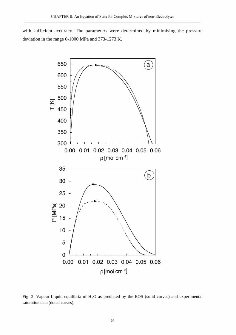
CHAPTER II. An Equation of State for Complex Mixtures of non-Electrolytes————————————————————————————————————————————————————————
76
with sufficient accuracy. The parameters were determined by minimising the pressure
deviation in the range 0-1000 MPa and 373-1273 K.
Fig. 2. Vapour-Liquid equilibria of H2O as predicted by the EOS (solid curves) and experimental
saturation data (doted curves).
a
300
350
400
450
500
550
600
650
0.00 0.01 0.02 0.03 0.04 0.05 0.06
ρ cm-3
[mol ]
T[K]
b
0
5
10
15
20
25
30
35
0.00 0.01 0.02 0.03 0.04 0.05 0.06
P[M
Pa]
ρ cm-3
[mol ]
CHAPTER II. An Equation of State for Complex Mixtures of non-Electrolytes————————————————————————————————————————————————————————
77
For temperatures above 773.15 K the P-V-T properties of water can be accurately reproduced
assigning constant values of the EOS parameters:
σ [Å] = 2.926 (34)
ε/k [K] = 264.604 (35)
µ [D] = 2.09457 (36)
At lower temperatures, this set of parameters provides unsatisfactory results. It was
possible, however, to extend the application range of the EOS by introducing a temperature
dependency of the dipole moment µ and the Lennard-Jones parameter σ, while the parameter
ε remains constant identical to the high temperature value. A simple quadratic function is used
which reaches smoothly the high temperature parameters at 773.15 K. The following relations
for µ and σ for T < 773.15K were derived:
σ [Å] = 2.926 - 2.0996·10-7 × (T - 773.15)2 (37)
µ [D] = 2.09457 - 2.5887·10-6 × (T - 773.15)2 (38)
In Fig. 1 the molar volumes of water predicted by the EOS and the values provided by
Saul and Wagner (1989) are plotted between 373-1273 K. The agreement is good except for
the direct vicinity of the liquid-vapour equilibrium (LVE) and the near critical region. The
deviations are emphasised in Figs. 2a,b which show the calculated the LVE in comparison to
the saturation properties of real H2O. The derived EOS reproduces accurately the critical
density and the critical temperature (Fig. 2a) while the critical pressure (Fig. 2b) is
overestimated by 6.4 MPa. Due to this discrepancy the density of the saturated vapour is
overestimated and the density of the coexisting liquid is underestimated. However, Fig. 1
shows that at sufficient distance from these conditions the EOS provides accurate PVT-
properties.
The observed deviations have an influence on those thermodynamic quantities,
however, which are calculated using integrals of the volume or pressure (e.g. Gibbs free
energy or fugacity). Therefore any Gibbs free energy calculated for low temperaures and
pressures above 50 MPa will have constant offset from the correct value. At the critical
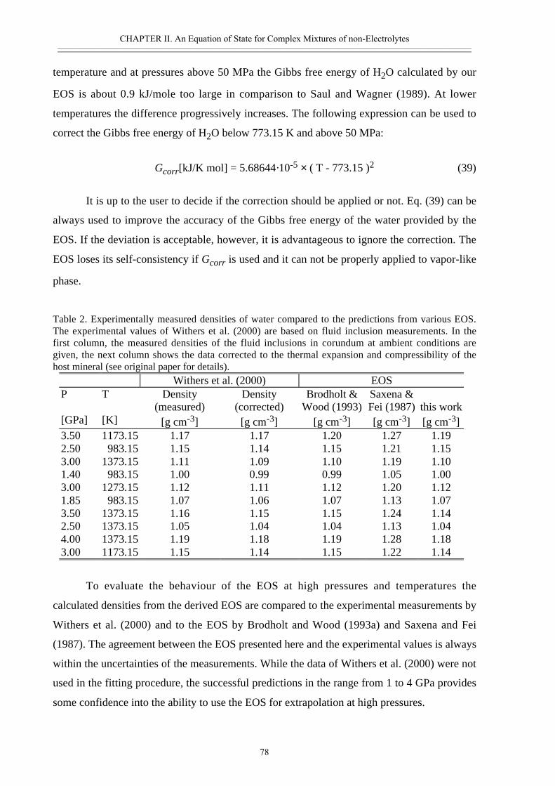
CHAPTER II. An Equation of State for Complex Mixtures of non-Electrolytes————————————————————————————————————————————————————————
78
temperature and at pressures above 50 MPa the Gibbs free energy of H2O calculated by our
EOS is about 0.9 kJ/mole too large in comparison to Saul and Wagner (1989). At lower
temperatures the difference progressively increases. The following expression can be used to
correct the Gibbs free energy of H2O below 773.15 K and above 50 MPa:
Gcorr[kJ/K mol] = 5.68644·10-5 × ( T - 773.15 )2 (39)
It is up to the user to decide if the correction should be applied or not. Eq. (39) can be
always used to improve the accuracy of the Gibbs free energy of the water provided by the
EOS. If the deviation is acceptable, however, it is advantageous to ignore the correction. The
EOS loses its self-consistency if Gcorr is used and it can not be properly applied to vapor-like
phase.
Table 2. Experimentally measured densities of water compared to the predictions from various EOS.The experimental values of Withers et al. (2000) are based on fluid inclusion measurements. In thefirst column, the measured densities of the fluid inclusions in corundum at ambient conditions aregiven, the next column shows the data corrected to the thermal expansion and compressibility of thehost mineral (see original paper for details).
Withers et al. (2000) EOSP
[GPa]
T
[K]
Density(measured)
[g cm-3]
Density(corrected)
[g cm-3]
Brodholt &Wood (1993)
[g cm-3]
Saxena &Fei (1987)[g cm-3]
this work[g cm-3]
3.50 1173.15 1.17 1.17 1.20 1.27 1.192.50 983.15 1.15 1.14 1.15 1.21 1.153.00 1373.15 1.11 1.09 1.10 1.19 1.101.40 983.15 1.00 0.99 0.99 1.05 1.003.00 1273.15 1.12 1.11 1.12 1.20 1.121.85 983.15 1.07 1.06 1.07 1.13 1.073.50 1373.15 1.16 1.15 1.15 1.24 1.142.50 1373.15 1.05 1.04 1.04 1.13 1.044.00 1373.15 1.19 1.18 1.19 1.28 1.183.00 1173.15 1.15 1.14 1.15 1.22 1.14
To evaluate the behaviour of the EOS at high pressures and temperatures the
calculated densities from the derived EOS are compared to the experimental measurements by
Withers et al. (2000) and to the EOS by Brodholt and Wood (1993a) and Saxena and Fei
(1987). The agreement between the EOS presented here and the experimental values is always
within the uncertainties of the measurements. While the data of Withers et al. (2000) were not
used in the fitting procedure, the successful predictions in the range from 1 to 4 GPa provides
some confidence into the ability to use the EOS for extrapolation at high pressures.
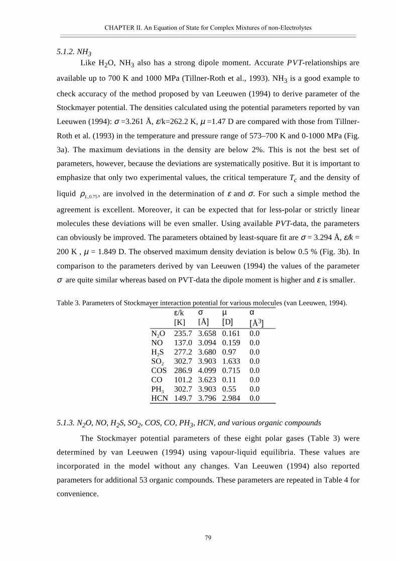
CHAPTER II. An Equation of State for Complex Mixtures of non-Electrolytes————————————————————————————————————————————————————————
79
5.1.2. NH3Like H2O, NH3 also has a strong dipole moment. Accurate PVT-relationships are
available up to 700 K and 1000 MPa (Tillner-Roth et al., 1993). NH3 is a good example to
check accuracy of the method proposed by van Leeuwen (1994) to derive parameter of the
Stockmayer potential. The densities calculated using the potential parameters reported by van
Leeuwen (1994): σ =3.261 Å, ε/k=262.2 K, µ =1.47 D are compared with those from Tillner-
Roth et al. (1993) in the temperature and pressure range of 573–700 K and 0-1000 MPa (Fig.
3a). The maximum deviations in the density are below 2%. This is not the best set of
parameters, however, because the deviations are systematically positive. But it is important to
emphasize that only two experimental values, the critical temperature Tc and the density of
liquid ρL, .0 75 , are involved in the determination of ε and σ. For such a simple method the
agreement is excellent. Moreover, it can be expected that for less-polar or strictly linear
molecules these deviations will be even smaller. Using available PVT-data, the parameters
can obviously be improved. The parameters obtained by least-square fit are σ = 3.294 Å, ε/k =
200 K , µ = 1.849 D. The observed maximum density deviation is below 0.5 % (Fig. 3b). In
comparison to the parameters derived by van Leeuwen (1994) the values of the parameter
σ are quite similar whereas based on PVT-data the dipole moment is higher and ε is smaller.
Table 3. Parameters of Stockmayer interaction potential for various molecules (van Leeuwen, 1994).
ε/k[K]
σ[Å]
µ[D]
α[Å3]
N2O 235.7 3.658 0.161 0.0NO 137.0 3.094 0.159 0.0H2S 277.2 3.680 0.97 0.0SO2 302.7 3.903 1.633 0.0COS 286.9 4.099 0.715 0.0CO 101.2 3.623 0.11 0.0PH3 302.7 3.903 0.55 0.0HCN 149.7 3.796 2.984 0.0
5.1.3. N2O, NO, H2S, SO2, COS, CO, PH3, HCN, and various organic compounds
The Stockmayer potential parameters of these eight polar gases (Table 3) were
determined by van Leeuwen (1994) using vapour-liquid equilibria. These values are
incorporated in the model without any changes. Van Leeuwen (1994) also reported
parameters for additional 53 organic compounds. These parameters are repeated in Table 4 for
convenience.
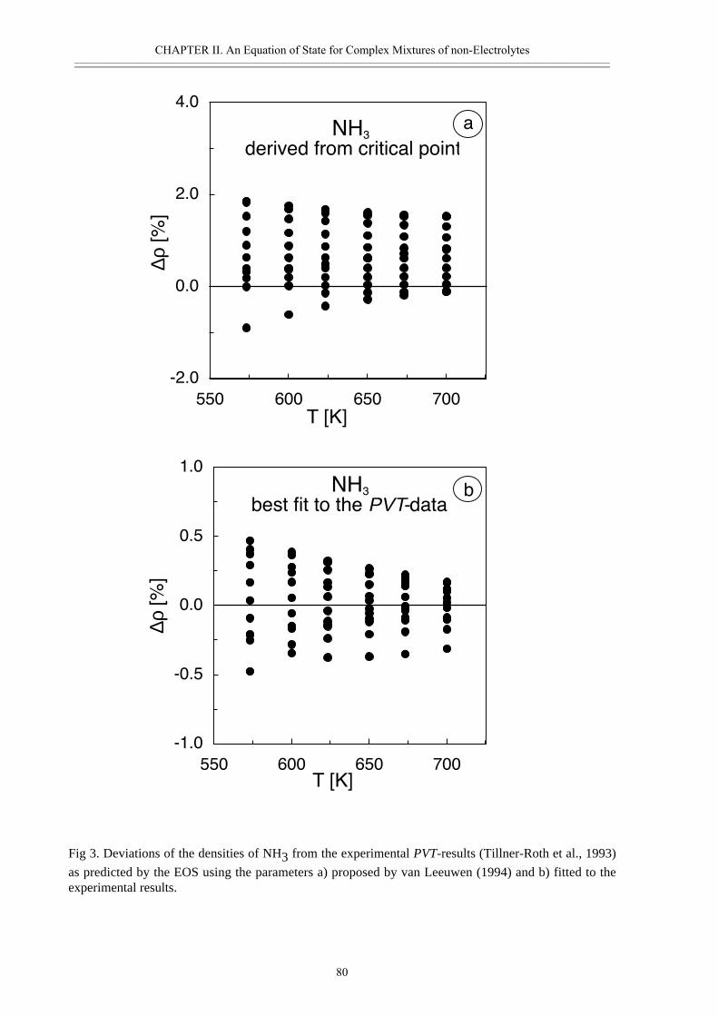
CHAPTER II. An Equation of State for Complex Mixtures of non-Electrolytes————————————————————————————————————————————————————————
80
Fig 3. Deviations of the densities of NH3 from the experimental PVT-results (Tillner-Roth et al., 1993)
as predicted by the EOS using the parameters a) proposed by van Leeuwen (1994) and b) fitted to theexperimental results.
NH3
best fit to the PVT-data
-1.0
-0.5
0.0
0.5
1.0
550 600 650 700T [K]
∆ρ [%
]
b
NH3
derived from critical point
-2.0
0.0
2.0
4.0
550 600 650 700T [K]
∆ρ[%
]
a

CHAPTER II. An Equation of State for Complex Mixtures of non-Electrolytes————————————————————————————————————————————————————————
81
Tab
le 4
. Par
amet
ers
for
furt
her
mol
ecul
es (
van
Lee
uwen
, 199
4).
ε/k
[K]
σ [Å]
µ [D]
α [Å3 ]
ε/k
[K]
σ [Å]
µ [D]
α [Å3 ]
CC
l 2O
(pho
sgen
e)34
2.3
4.54
81.
170.
0C
2H4O
(eth
ylen
e et
her)
324.
74.
079
1.89
0.0
CH
4O(m
etha
nol )
359
3.80
30.
710.
0C
4H8O
(tet
rahy
drof
uran
)40
3.4
4.85
61.
630.
0C
2H6O
(eth
anol
)37
3.3
4.29
90.
730.
0C
H5N
(met
hyla
min
e )
315.
13.
911.
290.
0C
3H8O
(n-p
ropa
nol )
398.
14.
691
0.69
0.0
C2H
7N(d
imet
hyla
inin
e)32
9.8
4.44
41.
030.
0C
3H8O
(2-p
ropa
nol )
376.
84.
699
0.66
0.0
C3H
9N(t
rim
ethy
lam
ine
)32
9.4
4.91
80.
630.
0C
4H10
O(n
-but
anol
)42
1.8
5.04
70.
660.
0C
2H7N
(eth
ylam
ine
)34
2.1
4.43
11.
220.
0C
4H10
O(2
-but
anol
)40
1.1
5.03
70.
660.
0C
4H11
N(d
ieth
ylam
ine)
377.
25.
212
0.91
0.0
C4H
10O
(2-m
ethy
l-1-
prop
anol
)41
0.4
5.04
10.
640.
0C
6H15
N(t
rim
etyl
amin
e)40
75.
798
0.83
0.0
C4H
10O
(2-m
ethy
l-2-
prop
anol
)37
8.1
5.06
10.
670.
0C
H3N
O2
(nitr
omet
hane
)29
0.4
4.34
73.
570.
0C
6H6O
(phe
nol )
524.
95,
079
1.45
0.0
C2H
3N(a
ceto
nitr
ile )
175.
74.
284
3.92
0.0
C3H
6O(a
ceto
ne)
326.
24.
691
2.88
0.0
C3H
3N(a
cryl
onitr
ile )
244.
34,
606
3.87
0.0
C4H
8O(2
-but
anon
e )
370.
45.
036
2.8
0.0
C5H
5N(p
yrid
ine
)45
3.3
4.95
62.
250.
0C
5H10
O(2
-pen
tano
ne )
402.
55.
382.
720.
0C
H4S
(met
hyl m
erca
ptan
)34
3.7
4.19
1.52
0.0
C5H
10O
(3-p
enta
none
)40
1.9
5.34
52.
720.
0C
2H6S
(dim
ethy
l sul
phid
e)37
5.1
4.63
71.
50.
0C
5H10
O(3
-met
hyl-
2-bu
tano
ne)
393.
95.
338
2.77
0.0
C2H
6S(e
thyl
mer
capt
an)
371.
24.
659
1.56
0.0
CH
2O(f
orm
alde
hyde
)20
6.5
3.73
12.
330.
0C
H3F
(flu
orom
etha
ne )
186.
73.
766
1.82
0.0
C2H
4O(a
cete
ldeh
yde
)26
8.3
4.24
82.
690.
0C
H2F
2(d
iflu
orom
etha
ne)
213
3.88
11.
960.
0C
3H6O
(pro
pion
alde
hyde
)33
5.5
4.64
82.
520.
0C
HF 3
(tri
fluo
rom
etha
ne)
199.
64.
007
1.62
0.0
C2H
4O2
(ace
tic a
cid)
435.
64.
356
1.74
0.0
C2H
5F(f
luor
oeth
ane
)25
3.3
4.26
81.
940.
0C
2H4O
2(m
ethy
l For
mat
e)35
2.6
4.37
41.
770.
0C
2H4F
2(1
,1-d
iflu
oroe
than
e)24
8.5
4.42
92.
30.
0C
3H6O
2(e
thyl
for
mat
e)37
1.9
4.80
60.
940.
0C
2H3F
3(1
,1,1
-tri
fluo
roet
hane
)22
1.2
4.53
52.
280.
0C
4H8O
2(n
-pro
pyl f
orm
ate)
402.
95.
159
0.7
0.0
CH
3CI
(chl
orom
etha
ne)
279.
84.
097
1.94
0.0
C3H
6O2
(Mm
ethy
l ace
tate
)37
6.3
4.78
10.
670.
0C
HC
I 3(t
rich
loro
met
hane
)40
6.5
4.82
91.
050.
0C
4H8O
2(e
thyl
ace
tate
)39
0.3
5.15
30.
780.
0C
2H4C
l 2(l
,l-di
clilo
roet
haiie
)38
1.7
4.9
2.06
0.0
C2H
6O(d
imet
hyl e
ther
)29
7.1
4.38
60.
30.
0C
6H5C
I(c
hlor
oben
zene
)47
6.3
5.31
91.
690.
0C
3H8O
(met
hyl e
thyl
eth
er)
329.
54.
793
0.23
0.0
C2H
5Br
(bro
moe
than
e )
370.
24.
684
1.79
0.0
C4H
10O
(die
thyl
eth
er)
353.
45.
166
0.13
0.0
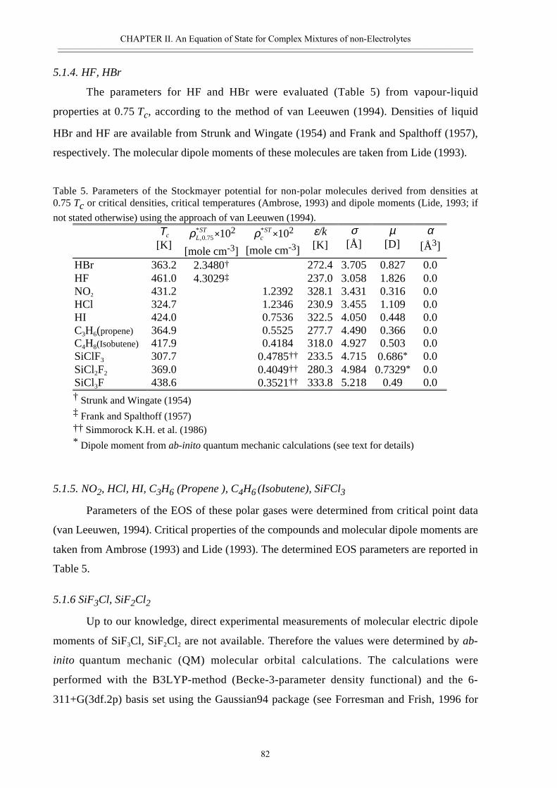
CHAPTER II. An Equation of State for Complex Mixtures of non-Electrolytes————————————————————————————————————————————————————————
82
5.1.4. HF, HBr
The parameters for HF and HBr were evaluated (Table 5) from vapour-liquid
properties at 0.75 Tc, according to the method of van Leeuwen (1994). Densities of liquid
HBr and HF are available from Strunk and Wingate (1954) and Frank and Spalthoff (1957),
respectively. The molecular dipole moments of these molecules are taken from Lide (1993).
Table 5. Parameters of the Stockmayer potential for non-polar molecules derived from densities at0.75 Tc or critical densities, critical temperatures (Ambrose, 1993) and dipole moments (Lide, 1993; if
not stated otherwise) using the approach of van Leeuwen (1994).
Τc
[K]ρL
ST, .
*0 75×102
[mole cm-3]
ρcST* ×102
[mole cm-3]
ε/k[K]
σ[Å]
µ[D]
α[Å3]
HBr 363.2 2.3480† 272.4 3.705 0.827 0.0HF 461.0 4.3029‡ 237.0 3.058 1.826 0.0NO2 431.2 1.2392 328.1 3.431 0.316 0.0HCl 324.7 1.2346 230.9 3.455 1.109 0.0HI 424.0 0.7536 322.5 4.050 0.448 0.0C3H6(propene) 364.9 0.5525 277.7 4.490 0.366 0.0C4H8(Isobutene) 417.9 0.4184 318.0 4.927 0.503 0.0SiClF3 307.7 0.4785†† 233.5 4.715 0.686* 0.0SiCl2F2 369.0 0.4049†† 280.3 4.984 0.7329* 0.0SiCl3F 438.6 0.3521†† 333.8 5.218 0.49 0.0† Strunk and Wingate (1954)‡ Frank and Spalthoff (1957)†† Simmorock K.H. et al. (1986)* Dipole moment from ab-inito quantum mechanic calculations (see text for details)
5.1.5. NO2, HCl, HI, C3H6 (Propene ), C4H6 (Isobutene), SiFCl3
Parameters of the EOS of these polar gases were determined from critical point data
(van Leeuwen, 1994). Critical properties of the compounds and molecular dipole moments are
taken from Ambrose (1993) and Lide (1993). The determined EOS parameters are reported in
Table 5.
5.1.6 SiF3Cl, SiF2Cl2
Up to our knowledge, direct experimental measurements of molecular electric dipole
moments of SiF3Cl, SiF2Cl2 are not available. Therefore the values were determined by ab-
inito quantum mechanic (QM) molecular orbital calculations. The calculations were
performed with the B3LYP-method (Becke-3-parameter density functional) and the 6-
311+G(3df.2p) basis set using the Gaussian94 package (see Forresman and Frish, 1996 for
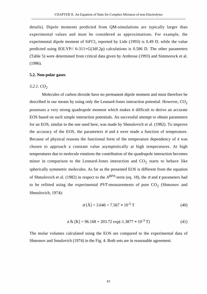
CHAPTER II. An Equation of State for Complex Mixtures of non-Electrolytes————————————————————————————————————————————————————————
83
details). Dipole moments predicted from QM-simulations are typically larger than
experimental values and must be considered as approximations. For example, the
experimental dipole moment of SiFCl3 reported by Lide (1993) is 0.49 D, while the value
predicted using B3LYP// 6-311+G(3df.2p) calculations is 0.586 D. The other parameters
(Table 5) were determined from critical data given by Ambrose (1993) and Simmorock et al.
(1986).
5.2. Non-polar gases
5.2.1. CO2
Molecules of carbon dioxide have no permanent dipole moment and must therefore be
described in our means by using only the Lennard-Jones interaction potential. However, CO2
possesses a very strong quadrupole moment which makes it difficult to derive an accurate
EOS based on such simple interaction potentials. An successful attempt to obtain parameters
for an EOS, similar to the one used here, was made by Shmulovich et al. (1982). To improve
the accuracy of the EOS, the parameters σ and ε were made a function of temperature.
Because of physical reasons the functional form of the temperature dependency of ε was
chosen to approach a constant value asymptotically at high temperatures. At high
temperatures due to molecule rotations the contribution of the quadrupole interaction becomes
minor in comparison to the Lennard-Jones interaction and CO2 starts to behave like
spherically symmetric molecules. As far as the presented EOS is different from the equation
of Shmulovich et al. (1982) in respect to the ARPA-term (eq. 18), the σ and ε parameters had
to be refitted using the experimental PVT-measurements of pure CO2 (Shmonov and
Shmulovich, 1974):
σ [Å] = 3.646 + 7.567 × 10⁻⁵ T (40)
ε /k [K] = 96.168 + 203.72 exp(-1.3877 × 10⁻³ T) (41)
The molar volumes calculated using the EOS are compared to the experimental data of
Shmonov and Smulovich (1974) in the Fig. 4. Both sets are in reasonable agreement.
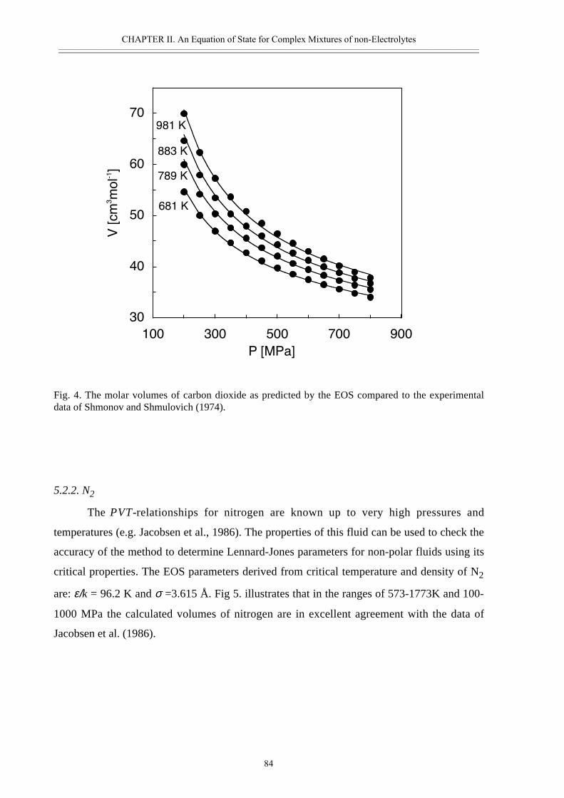
CHAPTER II. An Equation of State for Complex Mixtures of non-Electrolytes————————————————————————————————————————————————————————
84
Fig. 4. The molar volumes of carbon dioxide as predicted by the EOS compared to the experimentaldata of Shmonov and Shmulovich (1974).
5.2.2. N2
The PVT-relationships for nitrogen are known up to very high pressures and
temperatures (e.g. Jacobsen et al., 1986). The properties of this fluid can be used to check the
accuracy of the method to determine Lennard-Jones parameters for non-polar fluids using its
critical properties. The EOS parameters derived from critical temperature and density of N2
are: ε/k = 96.2 K and σ =3.615 Å. Fig 5. illustrates that in the ranges of 573-1773K and 100-
1000 MPa the calculated volumes of nitrogen are in excellent agreement with the data of
Jacobsen et al. (1986).
30
40
50
60
70
100 300 500 700 900
P [MPa]
V[cm
3mol-1]
681 K
789 K
883 K
981 K
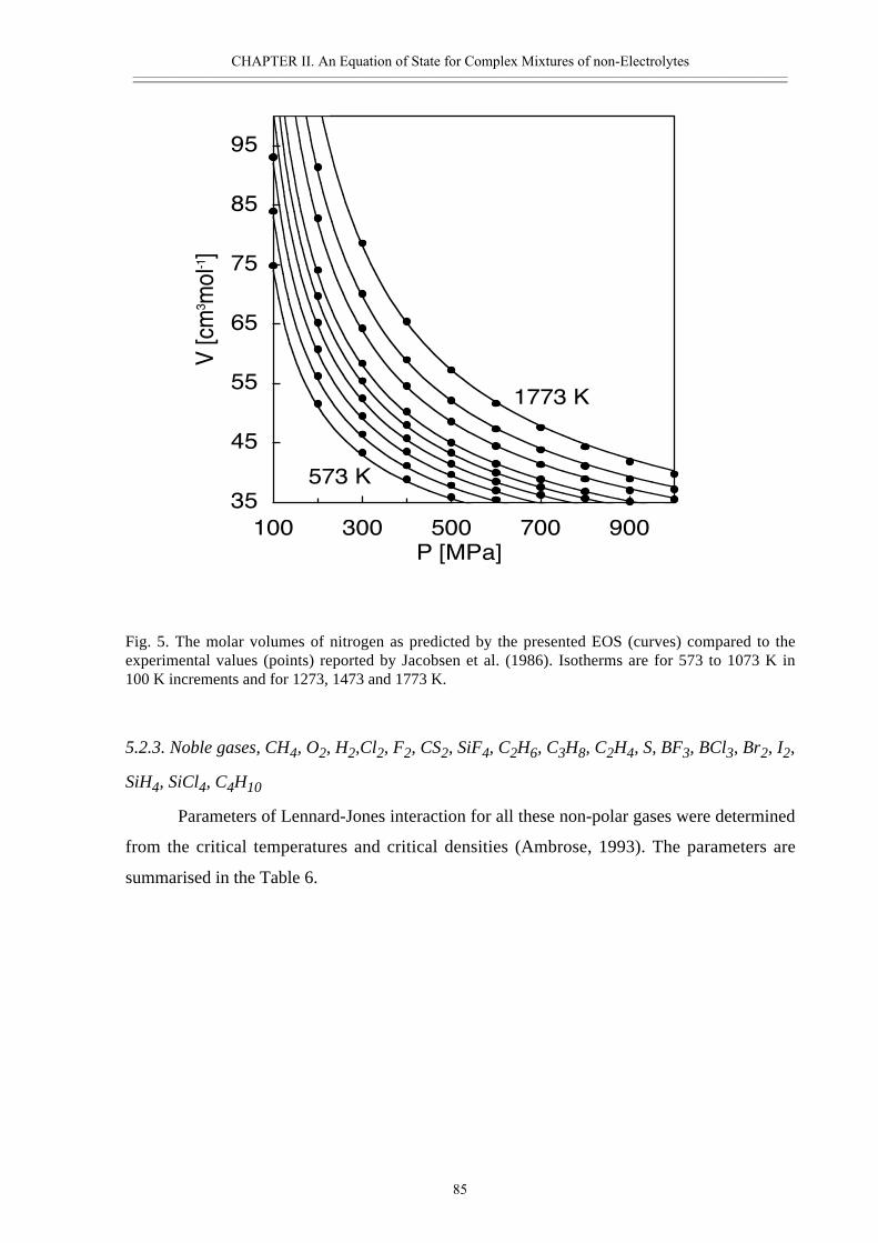
CHAPTER II. An Equation of State for Complex Mixtures of non-Electrolytes————————————————————————————————————————————————————————
85
Fig. 5. The molar volumes of nitrogen as predicted by the presented EOS (curves) compared to theexperimental values (points) reported by Jacobsen et al. (1986). Isotherms are for 573 to 1073 K in100 K increments and for 1273, 1473 and 1773 K.
5.2.3. Noble gases, CH4, O2, H2,Cl2, F2, CS2, SiF4, C2H6, C3H8, C2H4, S, BF3, BCl3, Br2, I2,
SiH4, SiCl4, C4H10
Parameters of Lennard-Jones interaction for all these non-polar gases were determined
from the critical temperatures and critical densities (Ambrose, 1993). The parameters are
summarised in the Table 6.
35
45
55
65
75
85
95
100 300 500 700 900
P [MPa]
V[cm
3mol-1]
573 K
1773 K
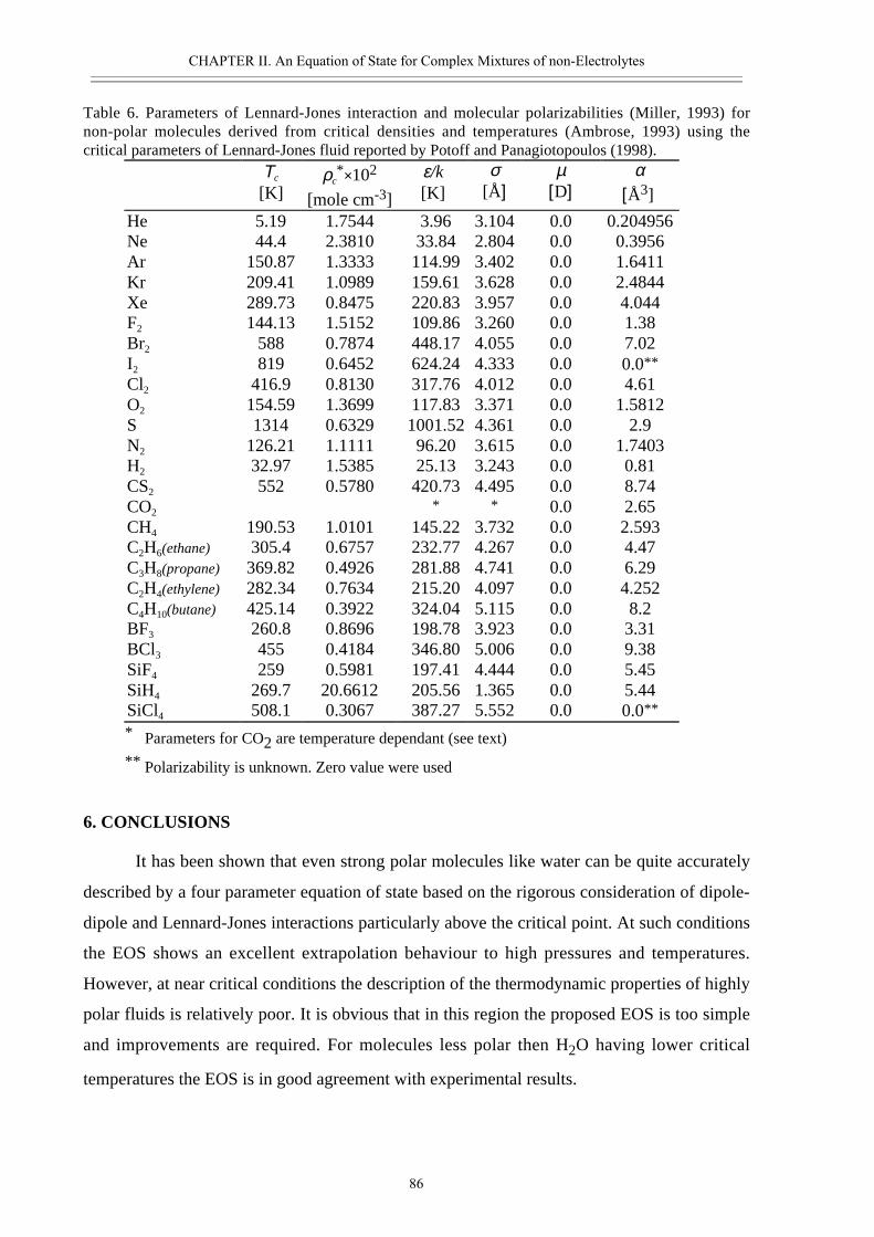
CHAPTER II. An Equation of State for Complex Mixtures of non-Electrolytes————————————————————————————————————————————————————————
86
Table 6. Parameters of Lennard-Jones interaction and molecular polarizabilities (Miller, 1993) fornon-polar molecules derived from critical densities and temperatures (Ambrose, 1993) using thecritical parameters of Lennard-Jones fluid reported by Potoff and Panagiotopoulos (1998).
Τc
[K]ρc
*×102
[mole cm-3]
ε/k[K]
σ[Å]
µ[D]
α[Å3]
He 5.19 1.7544 3.96 3.104 0.0 0.204956Ne 44.4 2.3810 33.84 2.804 0.0 0.3956Ar 150.87 1.3333 114.99 3.402 0.0 1.6411Kr 209.41 1.0989 159.61 3.628 0.0 2.4844Xe 289.73 0.8475 220.83 3.957 0.0 4.044F2 144.13 1.5152 109.86 3.260 0.0 1.38Br2 588 0.7874 448.17 4.055 0.0 7.02I2 819 0.6452 624.24 4.333 0.0 0.0**
Cl2 416.9 0.8130 317.76 4.012 0.0 4.61O2 154.59 1.3699 117.83 3.371 0.0 1.5812S 1314 0.6329 1001.52 4.361 0.0 2.9N2 126.21 1.1111 96.20 3.615 0.0 1.7403H2 32.97 1.5385 25.13 3.243 0.0 0.81CS2 552 0.5780 420.73 4.495 0.0 8.74CO2
* * 0.0 2.65CH4 190.53 1.0101 145.22 3.732 0.0 2.593C2H6(ethane) 305.4 0.6757 232.77 4.267 0.0 4.47C3H8(propane) 369.82 0.4926 281.88 4.741 0.0 6.29C2H4(ethylene) 282.34 0.7634 215.20 4.097 0.0 4.252C4H10(butane) 425.14 0.3922 324.04 5.115 0.0 8.2BF3 260.8 0.8696 198.78 3.923 0.0 3.31BCl3 455 0.4184 346.80 5.006 0.0 9.38SiF4 259 0.5981 197.41 4.444 0.0 5.45SiH4 269.7 20.6612 205.56 1.365 0.0 5.44SiCl4 508.1 0.3067 387.27 5.552 0.0 0.0**
* Parameters for CO2 are temperature dependant (see text)
** Polarizability is unknown. Zero value were used
6. CONCLUSIONS
It has been shown that even strong polar molecules like water can be quite accurately
described by a four parameter equation of state based on the rigorous consideration of dipole-
dipole and Lennard-Jones interactions particularly above the critical point. At such conditions
the EOS shows an excellent extrapolation behaviour to high pressures and temperatures.
However, at near critical conditions the description of the thermodynamic properties of highly
polar fluids is relatively poor. It is obvious that in this region the proposed EOS is too simple
and improvements are required. For molecules less polar then H2O having lower critical
temperatures the EOS is in good agreement with experimental results.

CHAPTER II. An Equation of State for Complex Mixtures of non-Electrolytes————————————————————————————————————————————————————————
87
Non-polar gases, with a relatively small quadrupole moment (e.g. N2) can be
successfully described by a Lennard-Jones fluid, with potential parameters derived from its
critical properties. Fluids of non-polar molecules with strong quadrupole moments are
difficult to describe by a simple Lennard-Jones model. Significant improvements can be
achieved, however, if the parameters used in the EOS depend on temperature.
Additionally, because the EOS describes a large number of species using the same
formalism it can be extended to complex mixtures which will be presented in a second part of
the communication (Churakov and Gottschalk, submitted to CGA).
Acknowledgment. The authors are grateful to A.G. Kalinichev for useful discussions and
kindly providing the source code for the EOS of a Lennard-Jones fluid.
REFERENCES
Ambrose D. (1993) Critical constants, boiling points and melting points of selected
compounds. In CRC Handbook of chemistry and Physics, (ed. D.R. Lide) CRC Press,
Boca Raton pp. 6/54-6/65.
Anderko, A., and Pitzer, K.S. (1993a) Equation-of-state representation of phase equilibria
and volumetric properties of the system NaCl-H2O above 573 K. Geochim.
Cosmochim. Acta 57, 1657-1680.
Anderko, A., and Pitzer, K.S. (1993b) Phase equilibria and volumetric properties of the
systems KCl-H2O and NaCl-KCL-H2O above 573 K: equation of state representation.
Geochim. Cosmochim. Acta 57, 4885-4897.
Andersen H. C., Chandler D. and Weeks J. D. (1972) Role of repulsive forces in liquids: The
optimized random phase approximation. J. Chem. Phys. 56, 3812-3823.
Belonoshko A. and Saxena S.K. (1991a) A molecular dynamic study of pressure-volume-
temperature properties of supercritical fluids: 1. H2O. Geochim. Cosmochim. Acta 55,
381-387.
Belonoshko A. and Saxena S.K. (1991b) A molecular dynamics study of the pressure-
volume-temperature poperties of supercritical fluids: 2. CO2, CH4, CO, O2 and H2.
Geochim. Cosmochim. Acta 55, 3191-3208.
Belonoshko A.B. and Saxena S.K. (1992) A unified equation of state for fluids of C-H-O-N-
S-Ar composition and their mixtures up to very high temperatures and pressures.
Geochim. Cosmochim. Acta 56, 3611-3626.
CHAPTER II. An Equation of State for Complex Mixtures of non-Electrolytes————————————————————————————————————————————————————————
88
Brodholt J. and Wood B. (1990) Molecular dynamics of water at high temperatures and
pressures. Geochim. Cosmochim. Acta 54, 2611-2616.
Brodholt J. and Wood B.(1993a) Simulation of the structure and thermodynamic properties of
water at high pressures and temperatures. J. Geophys. Res. 98, 519-536.
Brodholt J. and Wood B. (1993b) Molecular dynamics simulations of the properties of CO2 -
H2O mixtures at high pressures and temperatures. Amer. Miner. 78,.558-564.
Carnahan N.F. and Starling K.E. (1969) Equation of state for non-attracting rigid spheres. J.
Chem. Phys. 51, 635-636.
Churakov S.V. and Gottschalk M. (2001) Perturbation theory based equation of state for polar
molecular fluids. II. Fluid mixtures. Geochim. Cosmochim. Acta ( submitted )
Destrigneville C.M., Brodholt J.P. and Wood B.J. (1996) Monte Carlo simulation of H2O-
CO2 mixtures to 1073.15 K and 30 kbar. Chemical Geology 133, 53-65.
Dohrn R., Prausnitz J. M. (1990) A simple perturbation term for the Carnhan-Starling
equation of state. Fluid Phase Equilib. 61, 53 - 69.
Duan Z., Møller N. and Weare J. H. (1992a) An equation of state for the CH4-CO2-H2O
system: I. Pure systems from 0 to 1000°C and 0 and to 8000 bar. Geochim.
Cosmochim. Acta 56, 2605 - 2617
Duan Z., Møller N and Weare J. H. (1992b) An equation of state for the CH4-CO2-H2O
system: II, Mixtures from 50 to 1000°C and 0 to 1000 bar. Geochim. Cosmochim. Acta
56, 2619-2631.
Duan Z., Møller N. and Weare J. H. (1992c) Molecular dynamics simulation of PVT
properties of geological fluids and a general equation of state of nonpolar and weakly
polar gases up to 20000 bar. Geochim. Cosmochim. Acta 56, 3839-3845.
Duan Z., Møller N. and Weare J. H. (1995a) Molecular dynamics equation of state for
nonpolar geochemical fluids. Geochim. Cosmochim. Acta 59, 1533–1538.
Duan, Z., Møller, N., and Weare, J.H. (1995b) Equation of state for the NaCl-H2O-CO2
system: prediction of phase equilibria and volumetric properties. Geochim.
Cosmochim. Acta 59, 2869-2882.
Duan Z., Møller N., Weare J. H. (1996) A general equation of state for supercritical fluid
mixtures and molecular dynamics simulation of mixture PVTX properties. Geochim.
Cosmochim. Acta 60, 1209-1216.
Duan Z. Møller N. and Weare J.H. (2000) Accurate prediction of the thermodynamic
properties of fluids in the system. H2O-CO2-CH4-N2 up to 2000K and 100 kbar from
CHAPTER II. An Equation of State for Complex Mixtures of non-Electrolytes————————————————————————————————————————————————————————
89
a corresponding states/one fluid equation of state. Geochim. Cosmochim Acta 64,
1069-1075.
Forresman J.B. and Frish A. (1996) Exploring chemistry with electronic structure methods.
Gaussian Inc., Pittsburgh.
Frank E.U. and Spalthoff W. (1957) Fluorwasserstoff I. Spezifische Wärme, Dampfdruck und
Dichte bis zu 300°C und 300 atm. Z. Electrochem 61, 348-357.
Gray C.G. and Gubbins K. E. (1984) Theory of molecular fluids. I. Fundamentals. Clarendon
Press, Oxford.
Grevel K. D. and Chatterjee N. D. (1992) A modified Redlich-Kwong equation of state for
H2-H2O fluid mixtures at high pressures and at temperatures above 400°C. Eur. J.
Mineral. 4, 1303-1310.
Gubbins K.E. and Twu C.H. (1978) Thermodynamics of polyatomic fluid mixtures. I. Theory,
Chem. Eng. Sci. 33, 863-878.
Halbach H. and Chatterjee N.D. (1982) An empirical Redlich-Kwong- type equation of state
for water to 1,000°C and 200 kbar. Contrib. to Mineral. Petrol. 79, 337-345.
Hirschfelder, J.O., Curtiss, C.F. and Bird, R.B. (1964) Molecular theory of gases and liquids.
John Wiley & Sons, New York.
Holland T. and Powell R. (1991) A compensated-Redlich-Kwong (CORK) equation for
volumes and fugacities of CO2 and H2O in the range 1 bar to 50 kbar and 100-1600°C.
Contrib. Mineral. Petrol. 109, 265-273.
Holloway, J.R. (1976) Fugacity and activity of molecular species in supercritical fluids. In
D.G. Fraser, Ed. Thermodynamics in Geology, p. 161-181, Dordrecht-Holland/Boston
Jacobs G.K. and Kerrick D.M. (1981) Methane: an equation of state with application to the
ternary system H2O-CO2-CH4. Geochim. Cosmochim. Acta 45, 607-614.
Jacobsen R.T., Stewart R.B. and Jahangiri, M. (1986) Thermodynamic properties of nitrogen
from the freezing line to 2000 K at pressures to 1000 MPa. J. Phys. Chem. Ref. Data
15, 735-909.
Jonson J.W. and Norton D. (1991) Critical phenomenon in the hydrothermal systems: state,
thermodynamic, electrostatic and transport properties of H2O in the critical region.
Amer. J. Sci. 291, 541-648.
Kalinichev A.G. and Heinzinger K. (1995) Molecular dynamic of supercritical water:
computer simulation of vibration spectra with the flexible BJH potential. Geochim.
Cosmochim. Acta 59, 641-650.
CHAPTER II. An Equation of State for Complex Mixtures of non-Electrolytes————————————————————————————————————————————————————————
90
Kerrick D. M. and Jacobs G.K. (1981) A modified Redlich-Kwong equation for H2O, CO2,
and H2O-CO2 mixtures at elevated pressures and temperatures. Amer. J. Sci. 281, 735-
767.
Leeuwen, van M.E. (1994) Derivation of Stockmayer potential parameters for polar fluids.
Fluid Phase Equilib. 99, 1-18.
Lide D. R. (1993) Dipole moment of molecules in the gas phase. In CRC Handbook of
chemistry and Physics, (ed. D.R. Lide) CRC Press, Boca Raton pp 9/42-9/50.
Miller T. M. (1993) Atomic and molecular polarizabilities. In CRC Handbook of chemistry
and Physics, (ed. D.R. Lide) CRC Press, Boca Raton, pp 10/192-10/204.
Miyano Y. and Masuoka H. (1984) Equation of state based on Weeks-Chandler-Andersen
perturbation theory. Fluid Phase Equilib. 18, 131-146.
Prausnitz, J. M., Lichtenthaler, R.N. and Azevedo, E.G. (1999) Molecular thermodynamics of
fluid-phase equilibria. Third edition, Prentice Hall, New Jersey.
Potoff J.J. and Panagiotopoulos A.Z. (1998). Critical Point and phase behaviour of the pure
fluids and a Lennard-Jones mixture. J. Chem. Phys. 109, 14-20.
Ree F.H. (1984) A statistical mechanical theory of chemical reacting multiphase mixtures:
Application to the detonation properties of PENT. J. Chem. Phys. 81, 1251-1263.
Saul A. and Wagner W. (1989) A fundamental equation for water covering the range from the
melting line to 1273 K at pressures up to 2500MPa. J. Chem. Phys Ref. Data 18, 1537-
1564.
Saxena S.K. and Fei Y. (1987) Fluids at crustal pressures and temperatures. I. Pure species.
Contrib. Mineral. Petrol. 95, 370-375.
Saxena S.K. and Fei Y. (1988) Fluid mixtures in the C-H-O system at high pressure and
temperature. Geochim. Cosmochim. Acta 52, 505-512.
Shmonov V.M. and Shmulovich K.I. (1974) Molar volumes and equation of state of CO2 at
100-1000°C and 2000-10000 bars. Doclady Acad. Science USSR 217, 206-209.
Simmorock K.H., Janowsky R. and Ohnesorge A. (1986) Critical data of pure substances.
DECHEMA, Frankfurt a.M.
Shmulovich K.I., Tereshchenko Ye.N. and Kalinichev A.G. (1982) An equation of state and
isochors for nonpolar gases to 2000K and 10 GPa. Geochem. Internat. 19, 49-64.
Stell G., Rasaiah J.C. and Narang H. (1972) Thermodynamic perturbation theory for simple
polar fluids. I. Mol. Phys. 23, 393-406.
CHAPTER II. An Equation of State for Complex Mixtures of non-Electrolytes————————————————————————————————————————————————————————
91
Stell G., Rasaiah J.C. and Narang H. (1974) Thermodynamic perturbation theory for simple
polar fluids. II. Mol. Phys. 27, 1393-1414.
Sterner S. M. and Pitzer K. S. (1994) An equation of state for carbon dioxide valid from zero
to extreme pressures. Contrib. Mineral. Petrol. 117, 362-374.
Strunk W.G. and Wingate W.H. (1954) Density of liquid hydrogen bromide. J. Am. Chem.
Soc. 76, 1025-1027.
Tereshchenko E.N., Kalinichev A.G., Shmulovich K.I. (1981) Application of the equation of
state of the Lennard-Jones fluid to density calculations under high pressures. In:
Equations of State under Extreme Conditions, Novosibirsk, ITPM SO AN SSSR, 12-
19 (in Russian).
Tillner-Roth R., Harms-Watzenberg F. and Baehr H.D., (1993) Eine neue
Fundamentalgleichung für Ammoniak. DKV-Tagungsbericht 20, 167-181.
Verlet L. and Weis J.J. (1972a) Perturbation theory for the thermodynamic properties of
simple liquids. Mol. Phys. 24, 1013 - 1024.
Verlet L. and Weis J.J. (1972b) Equilibrium theory of simple liquids. Phys Rev. 5, 939-952.
Weeks J. D., Chandler D. and Andersen H. C. (1971) Role of repulsive forces in determinig
the equilibrium structure of simple liquids. J. Chem. Phys, 54, 5237-5247.
Withers A.C., Kohn S.C., Brooker R.A. and Wood B.J. (2000) A new method for determining
the P-V-T properties of high-density H2O using NMR: Results at 1.4-4.0 GPa and 700-
1100°C. Geochim. Cosmochim. Acta 64, 1051-1057.
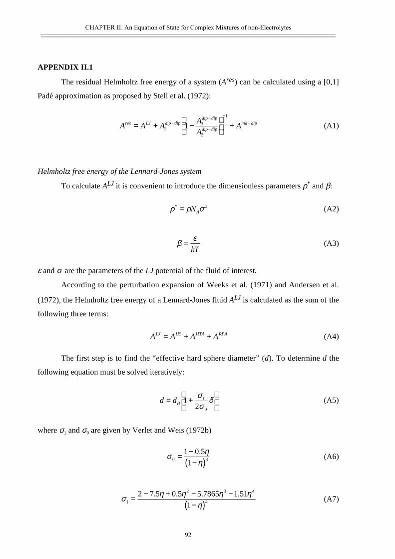
CHAPTER II. An Equation of State for Complex Mixtures of non-Electrolytes————————————————————————————————————————————————————————
92
APPENDIX II.1
The residual Helmholtz free energy of a system (Ares) can be calculated using a [0,1]
Padé approximation as proposed by Stell et al. (1972):
A A AA
AAres LJ dip dip
dip dip
dip dipind dip= + −
+−−
−
−−
23
2
1
11
(A1)
Helmholtz free energy of the Lennard-Jones system
To calculate ALJ it is convenient to introduce the dimensionless parameters ρ* and β:
ρ ρ σ* = NA3 (A2)
β ε=kT
(A3)
ε and σ are the parameters of the LJ potential of the fluid of interest.
According to the perturbation expansion of Weeks et al. (1971) and Andersen et al.
(1972), the Helmholtz free energy of a Lennard-Jones fluid ALJ is calculated as the sum of the
following three terms:
A A A ALJ HS HTA RPA= + + (A4)
The first step is to find the “effective hard sphere diameter” (d). To determine d the
following equation must be solved iteratively:
d dB= +
1
21
0
σσ
δ (A5)
where σ1 and σ0 are given by Verlet and Weis (1972b)
σ ηη0 3
1 0 5
1= −
−( ).
(A6)
σ η η η ηη1
2 3 4
4
2 7 5 0 5 5 7865 1 51
1= − + − −
−( ). . . .
(A7)
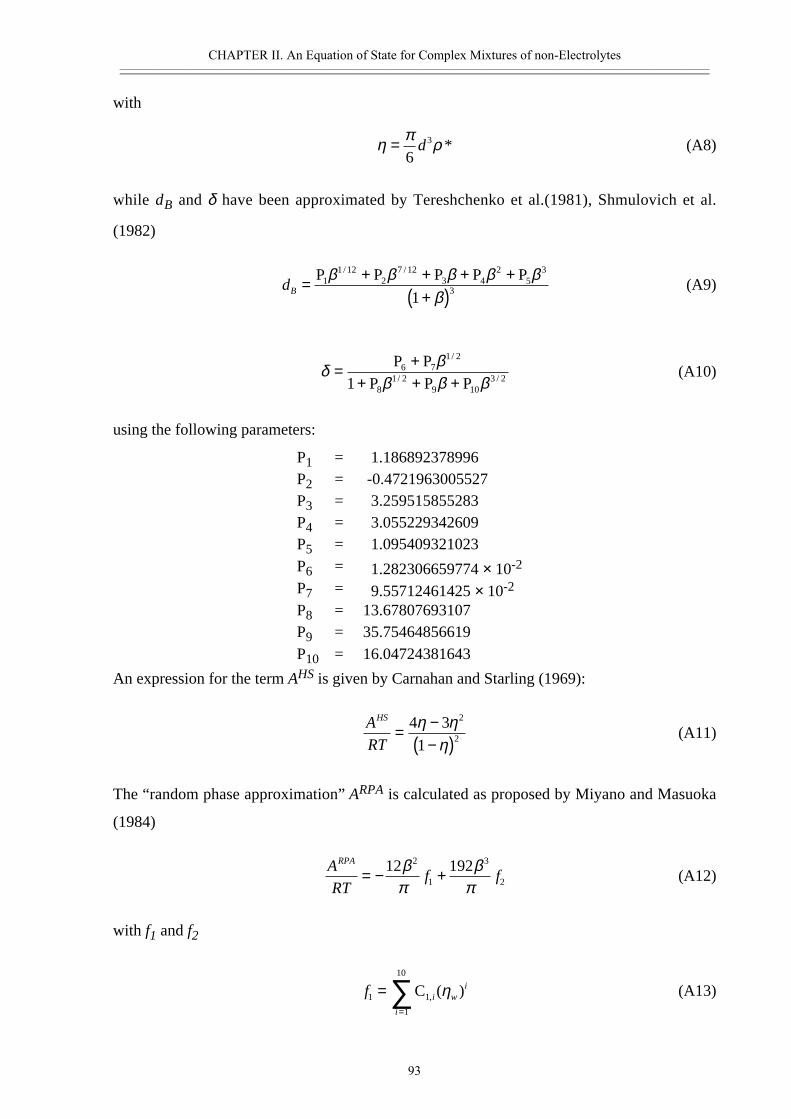
CHAPTER II. An Equation of State for Complex Mixtures of non-Electrolytes————————————————————————————————————————————————————————
93
with
η π ρ=6
3d * (A8)
while dB and δ have been approximated by Tereshchenko et al.(1981), Shmulovich et al.
(1982)
dB = + + + ++( )
P P P P P1 2 3 4 5β β β β ββ
1 12 7 12 2 3
31
/ /
(A9)
δ ββ β β
= ++ + +
P P1 P P P
6 7
8 9 10
1 2
1 2 3 2
/
/ / (A10)
using the following parameters:
P1 = 1.186892378996P2 = -0.4721963005527P3 = 3.259515855283P4 = 3.055229342609P5 = 1.095409321023P6 = 1.282306659774 × 10⁻²
P7 = 9.55712461425 × 10⁻²
P8 = 13.67807693107P9 = 35.75464856619P10 = 16.04724381643
An expression for the term AHS is given by Carnahan and Starling (1969):
A
RT
HS
= −−( )
4 3
1
2
2
η ηη
(A11)
The “random phase approximation” ARPA is calculated as proposed by Miyano and Masuoka
(1984)
A
RTf f
RPA
= − +12 1922
1
3
2
βπ
βπ
(A12)
with f1 and f2
f i wi
i
1 1
1
10
==∑C , ( )η (A13)
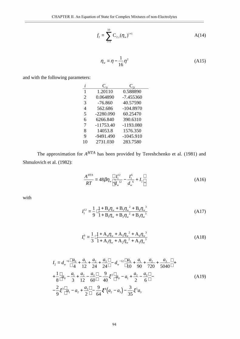
CHAPTER II. An Equation of State for Complex Mixtures of non-Electrolytes————————————————————————————————————————————————————————
94
f i wi
i
2 21
1
10
= +
=∑C , ( )η A(14)
η η ηw = − 116
2 (A15)
and with the following parameters:
i C1i C2i
1 1.20110 0.5888902 0.064890 -7.4553603 -76.860 40.575904 562.686 -104.89705 -2280.090 60.254706 6266.840 390.63107 -11753.40 -1193.0808 14053.8 1576.3509 -9491.490 -1045.910
10 2731.030 283.7580
The approximation for AHTA has been provided by Tereshchenko et al. (1981) and
Shmulovich et al. (1982):
A
RT
I
d
I
dI
HTA
ww w
= − +
48 1
12
1216
6 2βη (A16)
with
I w w w
w w w112
2 3
2 3
19
11
= ⋅ + + ++ + +
B B BB B B
4 5 6
1 2 3
η η ηη η η
(A17)
I w w w
w w w16
2 3
2 3
13
11
= ⋅ + + ++ + +
A A AA A A
4 5 6
1 2 3
η η ηη η η
(A18)
I da a a a
da a a a
aa a a
a aa a
a aa
w w26 0 1 2 3 12 0 1 2 3
01 2 3 2
0 12 3
31 2
3
4 12 24 24 10 90 720 5040
18 3 12 60
940 2 6
29 2
964
= + + +
− + + +
+
+ − + −
− − + −
−
− − +
−
− −
ξ
ξ ξξ ξ42 3
53
335
a a a−( ) −
(A19)
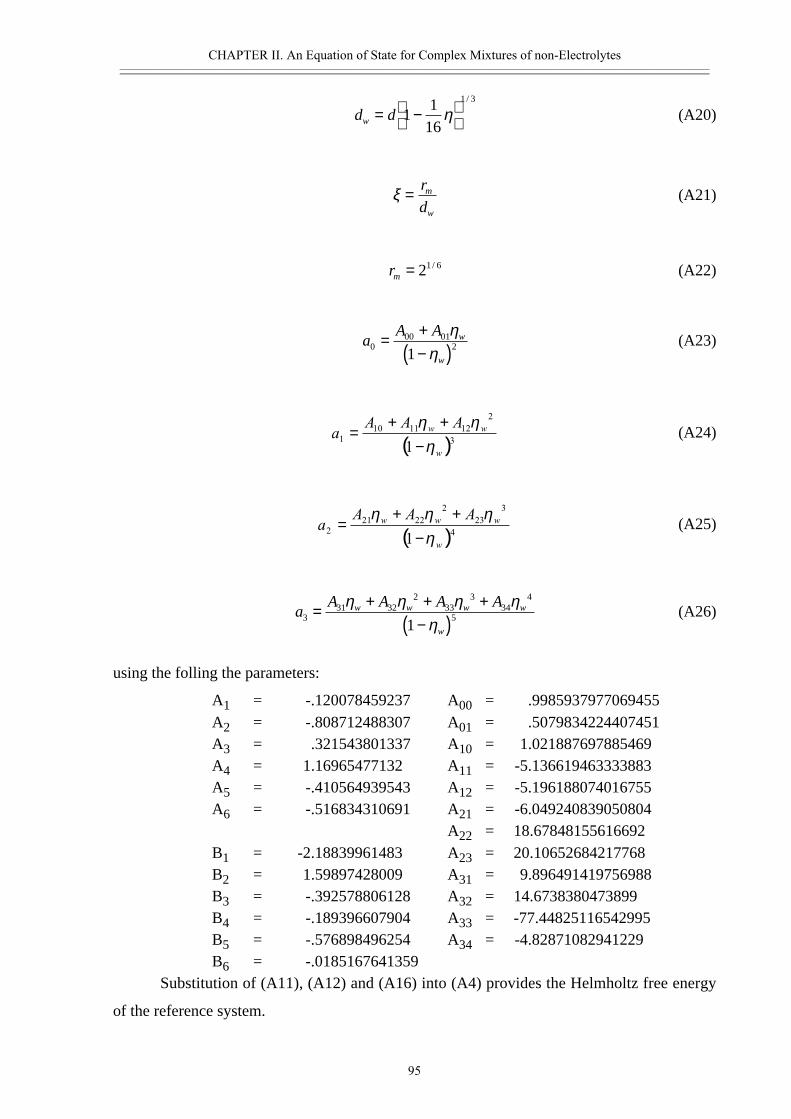
CHAPTER II. An Equation of State for Complex Mixtures of non-Electrolytes————————————————————————————————————————————————————————
95
d dw = −
1
116
1 3
η/
(A20)
ξ = r
dm
w
(A21)
rm = 21 6/ (A22)
aA A w
w
000 01
21
= +−( )
ηη
(A23)
( )3
2121110
11 w
ww AAAa
ηηη
−++
= (A24)
( )4
323
22221
21 w
www AAAa
ηηηη
−++
= (A25)
aA A A Aw w w w
w
331 32
233
334
4
51
= + + +−( )
η η η ηη
(A26)
using the folling the parameters:
A1 = -.120078459237 A00 = .9985937977069455A2 = -.808712488307 A01 = .5079834224407451A3 = .321543801337 A10 = 1.021887697885469A4 = 1.16965477132 A11 = -5.136619463333883A5 = -.410564939543 A12 = -5.196188074016755A6 = -.516834310691 A21 = -6.049240839050804
A22 = 18.67848155616692B1 = -2.18839961483 A23 = 20.10652684217768B2 = 1.59897428009 A31 = 9.896491419756988B3 = -.392578806128 A32 = 14.6738380473899B4 = -.189396607904 A33 = -77.44825116542995B5 = -.576898496254 A34 = -4.82871082941229B6 = -.0185167641359
Substitution of (A11), (A12) and (A16) into (A4) provides the Helmholtz free energy
of the reference system.
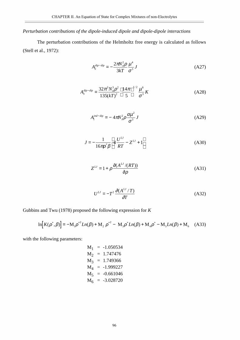
CHAPTER II. An Equation of State for Complex Mixtures of non-Electrolytes————————————————————————————————————————————————————————
96
Perturbation contributions of the dipole-induced dipole and dipole-dipole interactions
The perturbation contributions of the Helmholtz free energy is calculated as follows
(Stell et al., 1972):
AN
kTJdip dip A
2
2 4
3
23
− = − π ρ µσ
(A27)
AN
kTKdip dip A
3
3 3 2
2
1 2 6
3
32135
145
− =
π ρ π µσ( )
/
(A28)
A N Jind dipA12
2
34− = − π ραµσ
(A29)
JU
RTZ
LJLJ= − − +
116
4 1πρ β* (A30)
ZA RTLJ
LJ
= + ∂∂
1 ρρ
( /( ))(A31)
U TA T
TLJ
LJ
= − 2 ∂∂
( / )(A32)
Gubbins and Twu (1978) proposed the following expression for K
ln ( , ) ( ) ( ) ( )* * * * *K Ln Ln Lnρ β ρ β ρ ρ β ρ β[ ] = − + − + − +M M M M M M 1 2 3 4 5 6
2 2(A33)
with the following parameters:
M1 = -1.050534M2 = 1.747476M3 = 1.749366M4 = -1.999227M5 = -0.661046M6 = -3.028720

Perturbation Theory Based Equation of State for Polar Molecular Fluids:
II. Fluid Mixtures
CHAPTER II. An Equation of State for Complex Mixtures of non-Electrolytes————————————————————————————————————————————————————————
98
ABSTRACT
The equation of state (EOS) for 98 pure organic and inorganic fluids formulated by
Churakov and Gottschalk (submitted to GCA) has been extended to the complex fluid
mixtures. For the calculation of the thermodynamic properties of mixtures theoretical
combining rules from statistical mechanics are used. These mixing rules do not involve any
empirical parameters. The properties of the fluid mixtures are derived directly from those of
the pure constituents. It can be shown that the equation of state describes accurately the
thermodynamic relations in the H2O-CO2 and H2O-N2 binaries at high pressures and
temperatures. In particular the EOS correctly predicts high pressure phase separations in
various mixtures of polar and nonpolar molecules.
CHAPTER II. An Equation of State for Complex Mixtures of non-Electrolytes————————————————————————————————————————————————————————
99
1. INTRODUCTION
For many geological purposes, especially geothermobarometry, it seems to be
sufficient to consider H2O as the only fluid constituent. If carbonates are involved, however,
CO2 and at lower O2-fugacities other species like CH4, CO and H2 have to be considered
additionally. Besides CO2, N2-rich fluids have been found in many fluid inclusions in
granulite facies minerals (e.g. Touret and van den Kerkhof, 1986). Therefore fluids in lower
crust rocks have to be described at least within the system C-O-H-N. At special geological
conditions additional components like B, P, halogens, S, hydrocarbones and noble gases have
to be taken into account. For the treatment of such complex systems the thermodynamic
properties of the respective species in the mixture are essential. The equations of state (EOS),
which generally provides the required thermodynamic properties, are calibrated using the
following two approaches.
One is to use experimentally derived PVT-properties and/or activity relationships to
calibrate the EOS directly. Experimental studies, however, are in most cases limited to binary
systems (e.g. Seitz et al., 1994; Seitz et al., 1996a; Anovitz et al., 1998; Aranovich and
Newton, 1999; Constantino and Rice, 1991; Seward and Frank, 1981; Sterner and Bodnar
1991; Wu et al., 1990; Shmulovich et al., 1980). Few investigations have been done in
ternaries (e.g. Gehrig, 1980; Seitz et al., 1994; Seitz et al., 1996b). Because the number of
necessary experiments increases dramatically with the number of components, experimentally
determined PVT-properties of fluids with even more components are almost not available.
Due to this sparse experimental database directly calibrated EOS for complex fluids are rare.
Many experimentally calibrated EOS for mixtures involve ion pairs like NaCl and KCl which
have a very strong dipole moment and which can not be treated otherwise without difficulty.
Furthermore, because of dissociation even the simplest mixture like NaCl-H2O is essentually
not a binary system. It is very difficult to describe such systems theoretically. Therefore these
EOS use typically empirical parameters for the description of the mixing properties. The EOS
for the systems NaCl-H2O-CO2 (Bowers and Helgeson, 1983), NaCl-H2O (Anderko and
Pitzer, 1993a), KCl-H2O and NaCl-KCl-H2O (Anderko and Pitzer, 1993b) and NaCl-H2O-
CO2 (Duan et al. 1995b), H2O-CO2 (Sterner and Bodnar, 1991) do fall into this category.
Another approach is the use of an EOS for pure fluids and to interpolate the behaviour
of fluid mixtures applying mixing rules. This requires that for all species involved in the
mixture the EOS of the pure species are of the identical mathematical form, however.
CHAPTER II. An Equation of State for Complex Mixtures of non-Electrolytes————————————————————————————————————————————————————————
100
Significant efforts have been made to describe the thermodynamic properties of complex fluid
mixtures using such EOS (e.g. Holloway, 1976; Kerrick and Jacobs, 1981; Jacobs and
Kerrick, 1981; Saxena and Fei, 1988; Sretenskaya et al., 1989; Belonoshko and Saxena, 1992;
Grevel and Chatterjee, 1992; Duan et al., 1992, 1995a, 1995b, 1996, 2000; Bakker, 1999).
The choice of mixing rules is not unique. Many proposed mixing rules can be justified
theoretically using the conformal fluid theory (e.g. Prausnitz et al. 1999) and these can be
applied to many types of EOS (e.g. sophisticated forms of the van der Waals, virial equations
and equations based on perturbation theory). This however does not guaranty the accuracy of
the interpolation. A particular mixing model may work well for one fluid mixture but may fail
for another. In particular if a parameter in the EOS is temperature dependent, which is often
the case for semi-empirical EOS like modified van der Waals equations, mixing rules may
become inapplicable at some conditions. For example the application of mixing rules is
problematic if one of the coefficients describing the temperature dependency will be negative.
Often the square root (geometric mean) of the product of such coefficients is required.
EOS based on perturbation theory have been successfully applied to vapour-liquid
equilibria in various polar-non-polar gas systems using the generaliszed Stockmayer potential
(e.g. Stell et al., 1972, 1974; Gubbins and Twu, 1978; Twu and Gubbins, 1978). Gubbins and
Twu (1978) and Twu and Gubbins (1978) were able to mimic the different possible
topologies of phase equilibria in fluid mixtures by choosing the appropriate parameters for the
Lennard-Jones and multipolar interaction. The EOS just mentioned requires only mixing rules
for the reference Lennard-Jones system, but no additional rules for the perturbation term.
Furthermore the employed mixing rules for the reference system were verified by computer
simulations.
Churakov and Gottschalk (submitted to GCA) proposed an EOS for 98 pure fluids
which is also based on the Stockmayer interaction potential. In the following this EOS is
extended to fluid mixtures. It will be shown that the EOS can be used to predict the
thermodynamic properties of complex fluid mixtures up to high pressures and temperatures.
2. THERMODYNAMIC MODEL
In the following the EOS proposed by Churakov and Gottschalk (submitted to GCA)
is extended to fluid mixtures. Identical to the approach used for the pure fluids, the Helmholtz
free energy A is expressed in form of a truncated power expansion,
CHAPTER II. An Equation of State for Complex Mixtures of non-Electrolytes————————————————————————————————————————————————————————
101
A A A A A A Aideal res LJ dip dip dip dip ind dip− = = + + +− − −2 3 1
(1)
where ALJ is the residual Helmholtz free energy of a Lennard-Jones fluid which is used as the
reference system, Adip dip2
− and Adip dip3
− are the second and third order perturbation
contributions to the dipole-dipole interaction ( Adip dip1
− =0) and Aind dip
1
− is the first order
perturbation contribution to the induced dipole-dipole interaction.
According to Gubbins and Twu (1978) the explicit expressions for Adip dip2
− , Adip dip3
−
and Aind dip
1
− in the fluid mixture can be formulated as follows:
AN
kTx x Jdip dip A
i ji j
ijij
ij2
2 2 2
3
23
− = − ∑π ρ µ µσ
(2)
AN
kTx x x Kdip dip A
i j ki j k
ij ik jkijk
ijk3
3 3 2
2
1 2 2 2 232135
145
− =
∑π ρ π µ µ µ
σ σ σ( )
/
(3)
A N x x Jind dipA i j
iji j j i
ij
ij12
32 22
1− = − +∑π ρσ
α µ α µ( ) (4)
where xi is the mole fraction, µi the dipole moment and αi the polarizability of the molecule i,
ρ the fluid density, N the number of molecules, k the Boltzman constant and T the
temperature. The symbols Jij and Kijk are integrals over the pair and triple distribution
functions due to the interaction of two (i and j) and three molecules (i, j, and k) of the
reference Lennard-Jones fluid, which depend on temperature and density. For Jij and Kijk the
approximations of Stell et. al (1972) and Gubbins and Twu (1978) were used, respectively
(see Appendix II.2).
For a pure fluid consisting of the molecules i the calculation of ALJ, Adip dip2
− , Adip dip3
− ,
Aind dip
1
− , J and K requires the respective values for σi and εi because the molecular interactions
are all identical. In a mixture of molecules various interactions between different molecules (i
and j) have to be considered and therefore Lennard-Jones parameters σij and εij are necessary
for each i-j-pair of molecular interaction. These parameters can be approximated using the
standard Lohrentz-Bertholt combining rules:
σσ σ
iji j=+2
(5)
CHAPTER II. An Equation of State for Complex Mixtures of non-Electrolytes————————————————————————————————————————————————————————
102
ε ε εij i j= ( ) /1 2 (6)
No further approximations are necessary to calculate the perturbation contributions for
mixtures (eqs. 2-4).
The Lennard-Jones contributions to the mixture can be calculated using the van der
Waals one-fluid theory. The respective mixing parameters are calculated from the following
standard mixing rules, which are known to provide quite accurate results (Gray and Gubbins,
1984):
σ σ3 3mix i j ij
ij
x x= ∑ (7)
εσ
ε σmixmix
i j ij ij
ij
x x= ∑13
3 (8)
The corresponding values of the ε, σ, µ and α parameters for the pure components were
presented by Churakov and Gottschalk (submitted to GCA).
Finally, the fugacity coefficients ϕi of component i can be obtained by differentiation
of the Helmholtz free energy A=A(T,ρ, n1,n2,...) with respect to ni:
ln( )/
ln( ), ,
ϕ ii T V n
A RT
nZ Z
j i
= ∂∂
− + −≠
1 (9)
where ni is the number of moles of molecule i. The compressibility is obtained in the same
way as for the pure fluids:
ZA RTres
= + ∂∂
1 ρρ
( /( )). (10)
3. CALCULATED PROPERTIES IN THE SYSTEMS
H2O-CO2 , H2O-N2 AND H2O-CO2-CH4
Experimental determinations of PVT-properties of fluid mixtures at geological
relevant conditions are scarce. The H2O-CO2 binary is likely the best geologically relevant
system investigated over a wide range of pressures and temperatures. For example in the
range of intermediate pressures and temperatures the volumes of the H2O-CO2 have been
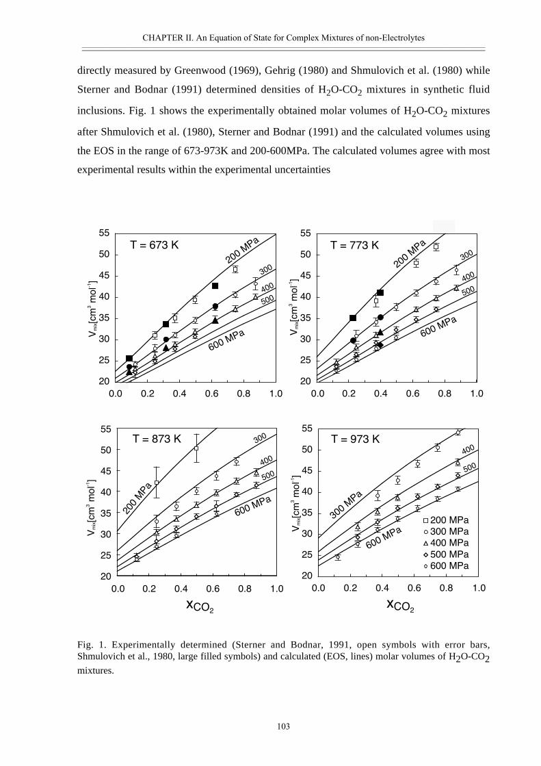
CHAPTER II. An Equation of State for Complex Mixtures of non-Electrolytes————————————————————————————————————————————————————————
103
directly measured by Greenwood (1969), Gehrig (1980) and Shmulovich et al. (1980) while
Sterner and Bodnar (1991) determined densities of H2O-CO2 mixtures in synthetic fluid
inclusions. Fig. 1 shows the experimentally obtained molar volumes of H2O-CO2 mixtures
after Shmulovich et al. (1980), Sterner and Bodnar (1991) and the calculated volumes using
the EOS in the range of 673-973K and 200-600MPa. The calculated volumes agree with most
experimental results within the experimental uncertainties
Fig. 1. Experimentally determined (Sterner and Bodnar, 1991, open symbols with error bars,Shmulovich et al., 1980, large filled symbols) and calculated (EOS, lines) molar volumes of H2O-CO2mixtures.
T = 873 K
20
25
30
35
40
45
50
55
0.0 0.2 0.4 0.6 0.8 1.0
Vmix[cm
3mol-1]
200 MPa
300 MPa
400 MPa
500 MPa
600 MPa
T = 973 K
20
25
30
35
40
45
50
55
0.0 0.2 0.4 0.6 0.8 1.0
Vmix[cm
3mol-1]
T = 773 K
20
25
30
35
40
45
50
55
0.0 0.2 0.4 0.6 0.8 1.0
Vmix[cm
3mol-1]
T = 673 K
20
25
30
35
40
45
50
55
0.0 0.2 0.4 0.6 0.8 1.0
Vmix[cm
3mol-1]
600MP
a
600 M
Pa
600 M
Pa
600 M
Pa
300MPa
200MPa
200MPa
200MPa
xCO2xCO2
300
400
500
300
400
500
300
400
500
400
500
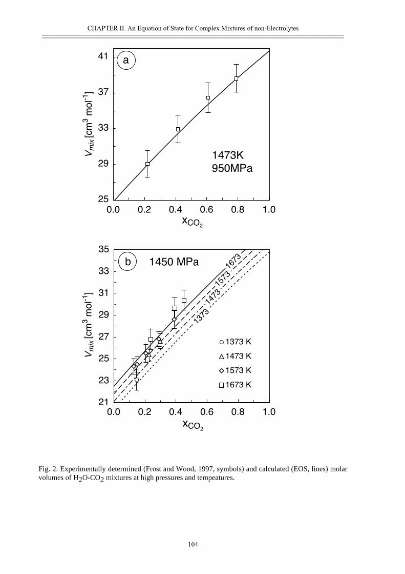
CHAPTER II. An Equation of State for Complex Mixtures of non-Electrolytes————————————————————————————————————————————————————————
104
Fig. 2. Experimentally determined (Frost and Wood, 1997, symbols) and calculated (EOS, lines) molarvolumes of H2O-CO2 mixtures at high pressures and tempeatures.
1450 MPa
21
23
25
27
29
31
33
35
0.0 0.2 0.4 0.6 0.8 1.0
1373 K
1473 K
1573 K
1673 K
1473K
950MPa
25
29
33
37
41
0.0 0.2 0.4 0.6 0.8 1.0
Vm
ix [cm
3mol-1]
Vm
ix [cm
3mol-1]
a
b
xCO2
xCO2
1673
1573
1473
1373
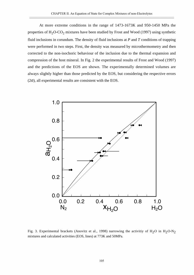
CHAPTER II. An Equation of State for Complex Mixtures of non-Electrolytes————————————————————————————————————————————————————————
105
At more extreme conditions in the range of 1473-1673K and 950-1450 MPa the
properties of H2O-CO2 mixtures have been studied by Frost and Wood (1997) using synthetic
fluid inclusions in corundum. The density of fluid inclusions at P and T conditions of trapping
were performed in two steps. First, the density was measured by microthermometry and then
corrected to the non-isochoric behaviour of the inclusion due to the thermal expansion and
compression of the host mineral. In Fig. 2 the experimental results of Frost and Wood (1997)
and the predictions of the EOS are shown. The experimentally determined volumes are
always slightly higher than those predicted by the EOS, but considering the respective errors
(2σ), all experimental results are consistent with the EOS.
Fig. 3. Experimental brackets (Anovitz et al., 1998) narrowing the activitiy of H2O in H2O-N2mixtures and calculated activities (EOS, lines) at 773K and 50MPa.
0.0 0.2 0.4 0.6 0.8 1.0
0.0
0.2
0.4
0.6
0.8
1.0
xH2O
aH2O
N2 H2O
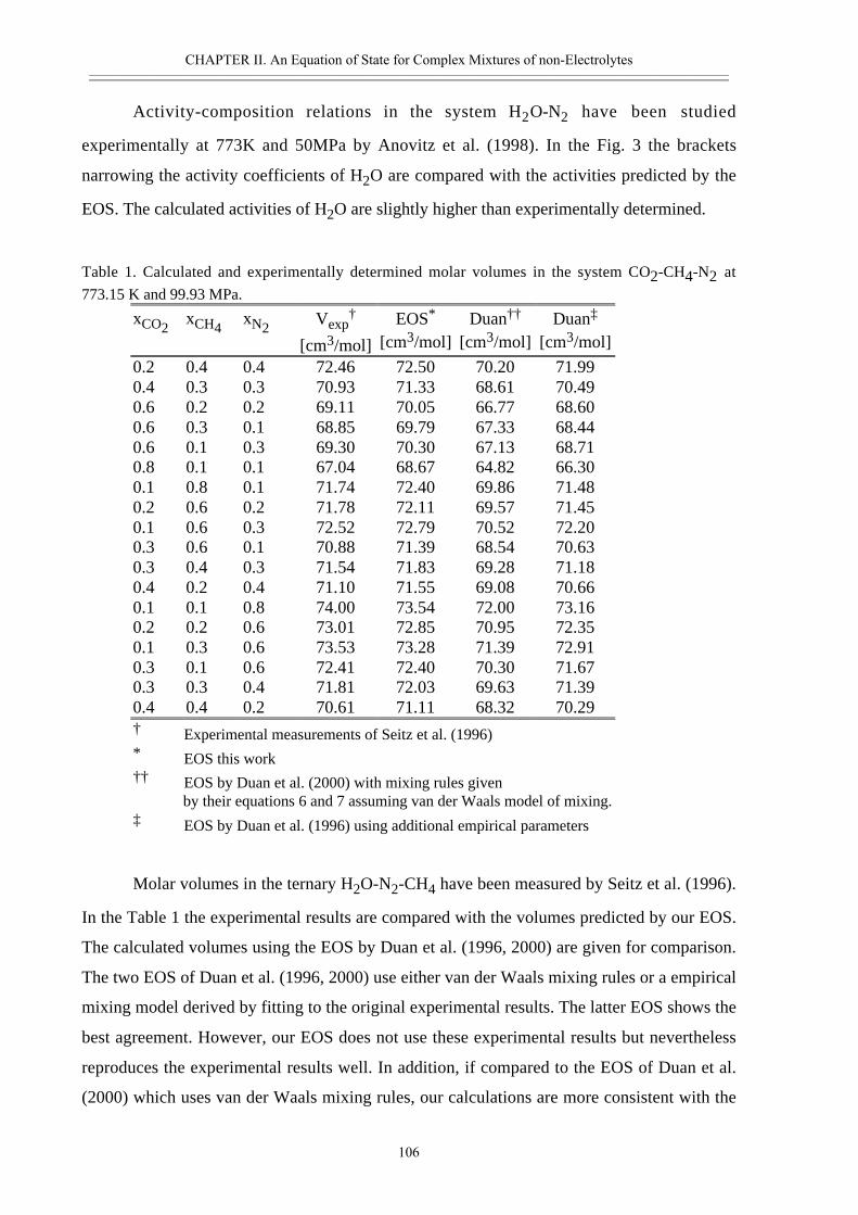
CHAPTER II. An Equation of State for Complex Mixtures of non-Electrolytes————————————————————————————————————————————————————————
106
Activity-composition relations in the system H2O-N2 have been studied
experimentally at 773K and 50MPa by Anovitz et al. (1998). In the Fig. 3 the brackets
narrowing the activity coefficients of H2O are compared with the activities predicted by the
EOS. The calculated activities of H2O are slightly higher than experimentally determined.
Table 1. Calculated and experimentally determined molar volumes in the system CO2-CH4-N2 at
773.15 K and 99.93 MPa.
xCO2xCH4
xN2Vexp
†
[cm3/mol]
EOS*
[cm3/mol]Duan††
[cm3/mol]Duan‡
[cm3/mol]
0.2 0.4 0.4 72.46 72.50 70.20 71.990.4 0.3 0.3 70.93 71.33 68.61 70.490.6 0.2 0.2 69.11 70.05 66.77 68.600.6 0.3 0.1 68.85 69.79 67.33 68.440.6 0.1 0.3 69.30 70.30 67.13 68.710.8 0.1 0.1 67.04 68.67 64.82 66.300.1 0.8 0.1 71.74 72.40 69.86 71.480.2 0.6 0.2 71.78 72.11 69.57 71.450.1 0.6 0.3 72.52 72.79 70.52 72.200.3 0.6 0.1 70.88 71.39 68.54 70.630.3 0.4 0.3 71.54 71.83 69.28 71.180.4 0.2 0.4 71.10 71.55 69.08 70.660.1 0.1 0.8 74.00 73.54 72.00 73.160.2 0.2 0.6 73.01 72.85 70.95 72.350.1 0.3 0.6 73.53 73.28 71.39 72.910.3 0.1 0.6 72.41 72.40 70.30 71.670.3 0.3 0.4 71.81 72.03 69.63 71.390.4 0.4 0.2 70.61 71.11 68.32 70.29† Experimental measurements of Seitz et al. (1996)* EOS this work†† EOS by Duan et al. (2000) with mixing rules given
by their equations 6 and 7 assuming van der Waals model of mixing.‡ EOS by Duan et al. (1996) using additional empirical parameters
Molar volumes in the ternary H2O-N2-CH4 have been measured by Seitz et al. (1996).
In the Table 1 the experimental results are compared with the volumes predicted by our EOS.
The calculated volumes using the EOS by Duan et al. (1996, 2000) are given for comparison.
The two EOS of Duan et al. (1996, 2000) use either van der Waals mixing rules or a empirical
mixing model derived by fitting to the original experimental results. The latter EOS shows the
best agreement. However, our EOS does not use these experimental results but nevertheless
reproduces the experimental results well. In addition, if compared to the EOS of Duan et al.
(2000) which uses van der Waals mixing rules, our calculations are more consistent with the
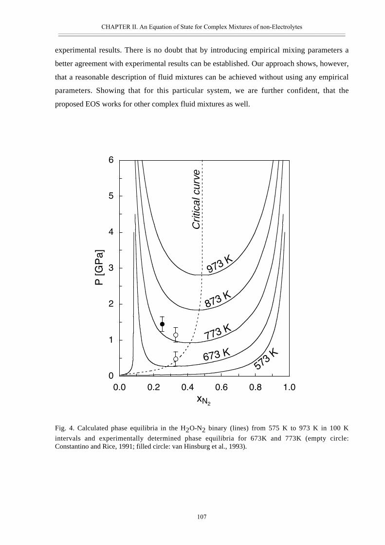
CHAPTER II. An Equation of State for Complex Mixtures of non-Electrolytes————————————————————————————————————————————————————————
107
experimental results. There is no doubt that by introducing empirical mixing parameters a
better agreement with experimental results can be established. Our approach shows, however,
that a reasonable description of fluid mixtures can be achieved without using any empirical
parameters. Showing that for this particular system, we are further confident, that the
proposed EOS works for other complex fluid mixtures as well.
Fig. 4. Calculated phase equilibria in the H2O-N2 binary (lines) from 575 K to 973 K in 100 K
intervals and experimentally determined phase equilibria for 673K and 773K (empty circle:Constantino and Rice, 1991; filled circle: van Hinsburg et al., 1993).
0
1
2
3
4
5
6
0.0 0.2 0.4 0.6 0.8 1.0
P[GPa]
xN2
Crit
ical
cur
ve
673 K
573K
873K
773K
973 K
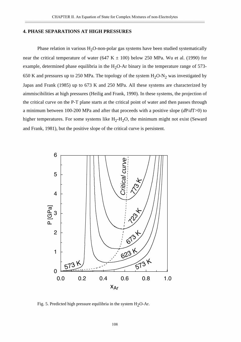
CHAPTER II. An Equation of State for Complex Mixtures of non-Electrolytes————————————————————————————————————————————————————————
108
4. PHASE SEPARATIONS AT HIGH PRESSURES
Phase relation in various H2O-non-polar gas systems have been studied systematically
near the critical temperature of water (647 K ± 100) below 250 MPa. Wu et al. (1990) for
example, determined phase equilibria in the H2O-Ar binary in the temperature range of 573-
650 K and pressures up to 250 MPa. The topology of the system H2O-N2 was investigated by
Japas and Frank (1985) up to 673 K and 250 MPa. All these systems are characterized by
aimmiscibilities at high pressures (Heilig and Frank, 1990). In these systems, the projection of
the critical curve on the P-T plane starts at the critical point of water and then passes through
a minimum between 100-200 MPa and after that proceeds with a positive slope (dP/dT>0) to
higher temperatures. For some systems like H2-H2O, the minimum might not exist (Seward
and Frank, 1981), but the positive slope of the critical curve is persistent.
Fig. 5. Predicted high pressure equilibria in the system H2O-Ar.
0
1
2
3
4
5
6
0.0 0.2 0.4 0.6 0.8 1.0
P[G
Pa]
xAr
623K
573 K
723K
673K
773K
573K
Crit
ical
cur
ve
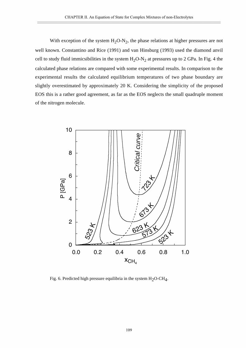
CHAPTER II. An Equation of State for Complex Mixtures of non-Electrolytes————————————————————————————————————————————————————————
109
With exception of the system H2O-N2, the phase relations at higher pressures are not
well known. Constantino and Rice (1991) and van Hinsburg (1993) used the diamond anvil
cell to study fluid immicsibilities in the system H2O-N2 at pressures up to 2 GPa. In Fig. 4 the
calculated phase relations are compared with some experimental results. In comparison to the
experimental results the calculated equilibrium temperatures of two phase boundary are
slightly overestimated by approximately 20 K. Considering the simplicity of the proposed
EOS this is a rather good agreement, as far as the EOS neglects the small quadruple moment
of the nitrogen molecule.
Fig. 6. Predicted high pressure equilibria in the system H2O-CH4.
0
2
4
6
8
10
0.0 0.2 0.4 0.6 0.8 1.0
P[GPa]
xCH4
573 K
523K
673K
623K
723K
Crit
ical
cur
ve
523K
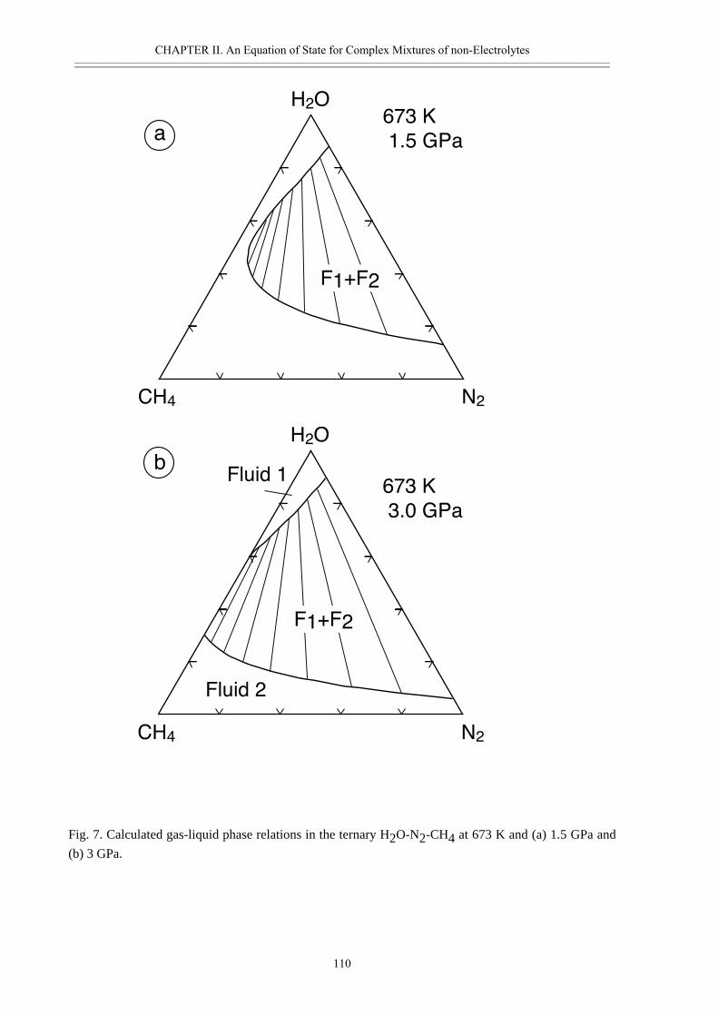
CHAPTER II. An Equation of State for Complex Mixtures of non-Electrolytes————————————————————————————————————————————————————————
110
Fig. 7. Calculated gas-liquid phase relations in the ternary H2O-N2-CH4 at 673 K and (a) 1.5 GPa and
(b) 3 GPa.
673 K
3.0 GPa
673 K
1.5 GPaa
b
CH4
H2O
N2
F1+F2
CH4
H2O
N2
Fluid 1
Fluid 2
F1+F2
CHAPTER II. An Equation of State for Complex Mixtures of non-Electrolytes————————————————————————————————————————————————————————
111
In Fig. 5 and Fig. 6 the calculated phase relations in the system H2O-Ar and H2O-CH4
are shown, respectively. These systems are characterized by a more ideal behaviour in
comparison to the H2O-N2 binary. Thus at 673K the predicted phase separation in the systems
H2O-Ar and H2O-CH4 would occur at pressures above 1 and 2 GPa, respectively. In the case
of systems with the three and more components the fluid equilibria inherit the phase relations
observed in the binary subsystems. The calculated phase equilibria in the H2O-N2-CH4
ternary are shown in the Fig. 7 for a temperature of 673 K and for pressures of 1.5 and 3 GPa,
respectively. According to the calculations, CH4 is more soluble in H2O than N2. At 1.5 GPa
a phase separation is predicted in the system H2O-N2 but not in the H2O-CH4 binary. In the
ternary a large two phase field separating a H2O-rich liquid and a N2-CH4-rich gas is
predicted. At 3 GPa the two phase field will extend over the whole ternary. It is interesting to
note, that independent on pressure the N2/CH4 ratio in both coexisting phases is
approximately identical and only the concentrations of the polar molecule in the two fluids is
substantially different.
5. CONCLUSIONS
The EOS based on the thermodynamic perturbation theory using a generalized
Stockmayer interaction potential has been applied to mixtures of strongly polar and non-polar
molecular fluids over a wide range of pressures and temperatures. The EOS reproduces the
experimental determined activity-composition relations accurately and high pressure phase
separations in the various fluid mixtures are predicted correctly without any empirical
parameters. The accuracy of the predicted thermodynamic properties for fluid mixtures
depends on the nature of the fluid, however. In comparison to fluids containing spherically
symmetric molecules like noble gases or slightly polar ones like CO, the accuracy is definitely
lower for fluids involving highly polar molecules like H2O or non-polar molecules with a
strong quadruple moment like CO2. An improvement could be obviously achieved if
quadruple and higher order multipolar interactions as well as anisotropic inductions and
dispersion forces would be explicitly included. It would be also desirable to apply a non-
spherical reference system to account for anisotropic molecules.
Acknowledgment. The authors are grateful to A.G. Kalinichev for useful discussions and
kindly providing the source code for the EOS of a Lennard-Jones fluid.
CHAPTER II. An Equation of State for Complex Mixtures of non-Electrolytes————————————————————————————————————————————————————————
112
REFERENCES
Anderko, A., and Pitzer, K.S. (1993a) Equation-of-state representation of phase equilibria and
volumetric properties of the system NaCl-H2O above 573 K. Geochim. Cosmochim.
Acta 57, 1657-1680.
Anderko A. and Pitzer K. S. (1993b) Phase equilibria and volumetric properties of the
systems KCl-H2O and NaCl-KCl-H2O above 573 K; equation of state representation.
Geochim. Cosmochim. Acta 57, 4885-4897.
Anovitz M.A., Blencoe J.G. Joyce D.B. and Horita J. (1998) Precise measurement of
activity/compositions of H2O-N2 and H2O-CO2 fluids at 500°C, 500 bars. Geochim.
Cosmochim. Acta 62, 815-829.
Aranovich L.Y. and Newton R.C. (1999) Experimental determination of CO2-H2O activity-
composition relations at 600-1000°C and 6-14 kbar by reversed decarbonation
dehydration reactions. Amer. Mineral. 84, 1319-1332.
Bakker R. J. (1999) Adaptation of the Bowers and Helgeson (1983) equation of state to the
H2O-CO2-CH4-N2-NaCl system. Chem. Geol. 154, 225-236.
Belonoshko A.B. and Saxena S.K. (1992) A unified equation of state for fluids of C-H-O-N-
S-Ar composition and their mixtures up to very high temperatures and pressures.
Geochim. Cosmochim. Acta 56, 3611-3626.
Bowers T. S. and Helgeson H. C. (1983) Calculation of the thermodynamic and geochemical
consequences of nonideal mixing in the system H2O-CO2-NaCl on phase relations in
geologic systems: Equation of state for H2O-CO2-NaCl fluids at high pressures
temperatures. Geochimica et Cosmochimica Acta 47, 1247-1275.
Churakov S.V. and Gottschalk M. (2001) Perturbation theory based equation of state for polar
molecular fluids. I. Pure fluids. Geochim. Cosmochim. Acta (submitted).
Constantino M. and Rice S.F. (1991) Supercritical phase separation in the H2O-N2 mixtures.
J. Chem. Phys. 95, 9034-9036.
Duan Z., Møller N. and Weare J. H. (1992) An equation of state for the CH4-CO2-H2O
system: II. mixtures from 50 to 1000°C and 0 to 1000 bar. Geochim. Cosmochim. Acta
56, 2619-2631.
Duan Z., Møller N. and Weare J. H. (1995a) Molecular dynamics equation of state for
nonpolar geochemical fluids. Geochim. Cosmochim. Acta 59, 1533–1538.
CHAPTER II. An Equation of State for Complex Mixtures of non-Electrolytes————————————————————————————————————————————————————————
113
Duan, Z., Møller, N., and Weare, J.H. (1995b) Equation of state for the NaCl-H2O-CO2
system: prediction of phase equilibria and volumetric properties. Geochim.
Cosmochim. Acta 59, 2869-2882.
Duan Z., Møller N. and Weare J. H. (1996) A general equation of state for supercritical fluid
mixtures and molecular dynamics simulation of mixture PVTX properties. Geochim.
Cosmochim. Acta 60, 1209-1216.
Duan Z. Møller N. and Weare J.H. (2000) Accurate prediction of the thermodynamic
properties of fluids in the system. H2O-CO2-CH4-N2 up to 2000K and 100 kbar from
a corresponding states/one fluid equation of state. Geochim. Cosmochim Acta 64,
1069-1075.
Frost D.J. and Wood B.J (1997) Experimental measurements of the properties of H2O-CO2
mixtures at high pressures and temperatures. Geochim. Cosmochim Acta 61, 3301-
3309
Gehrig M. (1980) Phasengleichgewichte und PVT-Daten ternärer Mischungen aus Wasser,
Kohlendioxid und Natriumchlorid. Dissertation, University Karlsruhe.
Gray C.G. and Gubbins K. E. (1984) Theory of molecular fluids. I. Fundamentals. Clarendon
Press, Oxford.
Greenwood H. J. (1969) The compressibility of gaseous mixtures of carbon dioxide and water
between 0 and 500 bars. Amer. Jour. Sci. 267A, 191-208.
Grevel K. D. and Chatterjee N. D. (1992) A modified Redlich-Kwong equation of state for
H2-H2O fluid mixtures at high pressures and at temperatures above 400°C. Eur. J.
Mineral. 4, 1303-1310.
Gubbins K.E. and Twu C.H. (1978) Thermodynamics of polyatomic fluid mixtures. I. Theory,
Chem. Eng. Sci. 33, 863-878.
Heilig M. and Frank E.U. (1990) Phase equilibria in the multicomponent fluid systems to high
pressure and temperature. Ber. Bunsenges Phys Chem. 94, 27-35.
Hinsburg van M.G.E. Verbrugge R. and Schouten J.A. (1993) High temperature high-pressure
experiments on H2O-N2. Fluid Phase Equilib. 88, 115-121
Holloway, J.R. (1976) Fugacity and activity of molecular species in supercritical fluids. In
D.G. Fraser, Ed. Thermodynamics in Geology, p. 161-181, Dordrecht-Holland/Boston
Jacobs G.K. and Kerrick D.M. (1981) Methane: an equation of state with application to the
ternary system H2O-CO2-CH4. Geochim. Cosmochim. Acta 45, 607-614.
CHAPTER II. An Equation of State for Complex Mixtures of non-Electrolytes————————————————————————————————————————————————————————
114
Japas M.L. and Franck E.U. (1985) High pressure phase equilibria and PVT-data of the water-
nitrogen system to 673 K and 250 MPa. Ber. Bunsenges. Phys. Chem. 89, 793-800.
Kerrick D. M. and Jacobs G.K. (1981) A modified Redlich-Kwong equation for H2O, CO2,
and H2O-CO2 mixtures at elevated pressures and temperatures. Amer. J. Sci. 281, 735-
767.
Prausnitz, J. M., Lichtenthaler, R.N. and Azevedo, E.G. (1999) Molecular thermodynamics of
fluid-phase equilibria. Third edition, Prentice Hall, New Jersey.
Saxena S.K. and Fei Y. (1988) Fluid mixtures in the C-H-O system at high pressure and
temperature. Geochim. Cosmochim. Acta 52, 505-512.
Seitz J.C., Blencoe J.G., Joyce D.B. and Bodnar J. R. (1994) Volumetric properties of CO2-
CH4-N2 fluids at 200°C and 1000 bars: A comparison of equations of state and
experimental data. Geochim. Cosmochim. Acta 58, 1065-1071.
Seitz J.C., Blencoe J.G. and Bodnar J. R. (1996a) Volumetric properties for {(1 - x)CO2 +
xCH4}, {(1 - x)CO2 + xN2}, and {(1 - x)CH4 + xN2} at the pressures (9.94, 19.94,
29.94, 39.94, 59.93, 79.93, and 99.93) MPa and temperatures (323.15, 373.15, 473.15,
and 573.15) K. J. Chem. Thermodyn. 28, 521-538.
Seitz J.C., Blencoe J.G. and Bodnar J. R. (1996b) Volumetric properties for {(x1CO2 + x2CH4
+ (1 - x1- x2)N2} at the pressures (19.94, 39.94, 59.93, 79.93, and 99.93) MPa and
temperatures (323.15, 373.15, 473.15, and 573.15) K. J. Chem. Thermodyn. 28, 539-
550.
Seward T.M. and Frank E.U. (1981) The system hydrogen-water up to 440°C and 2500 bar
pressure. Ber. Bunsengen. Phys. Chem, 85, 2-7
Shmulovich K.I., Shmonov V.M., Mazur V.A. and Kalinichev A.G. (1980) P-V-T and
activity concentration relations in the H2O-CO2 system (homogeneous solutions).
Geochem. Int. 17, 123-139.
Sretenskaya N.G., Razina M.V. and Belonozhko A.B. (1989) Calculation of thermodynamic
properties for the KCl-H2O system under high parameters using the modified Redlich-
Kwong equation. Geochem. Int. 26, 70-80.
Stell G., Rasaiah J.C. and Narang H. (1972) Thermodynamic perturbation theory for simple
polar fluids, I. Mol. Phys. 23, 393-406.
Stell G., Rasaiah J.C. and Narang H. (1974) Thermodynamic perturbation theory for simple
polar fluids, II. Mol. Phys. 27, 1393-1414.
CHAPTER II. An Equation of State for Complex Mixtures of non-Electrolytes————————————————————————————————————————————————————————
115
Sterner S.M. and Bodnar R.J. (1991) Synthetic fluid inclusions. X: Experimental
determination of P-V-T-X properties in the CO2-H2O system to 6kb and 700°C. Amer
J. Sci. 291, 1-54.
Touret J. and Kerkhof, van den A.M. (1986) High density fluids in the lower crust and upper
mantle. Physica 139 & 140B, 834-840.
Twu C.H. and Gubbins K.E. (1978) Thermodynamics of polyatomic fluid mixtures. II Polar,
quadrupolar, octopolar. Chem. Eng. Sci. 33, 879-887.
Wu G., Heileg M. Lentz H. and Frank E.U. (1990) High pressure phase equilibria in the
water-argon system. Ber. Bunsenges Phys Chem. 94, 27-35.
CHAPTER II. An Equation of State for Complex Mixtures of non-Electrolytes————————————————————————————————————————————————————————
116
APPENDIX II.2
The residual Helmholtz free energy of a system (Ares) can be calculated using a [0,1]
Padé approximation as proposed by Stell et al. (1972):
A A AA
AAres LJ dip dip
dip dip
dip dipind dip= + −
+−−
−
−−
23
2
1
11
(A1)
The appendix of Churakov and Gottschalk(submitted to GCA) treats the calculation of
the Helmholtz free energy of pure fluids. In the following the required additions needed to
treat fluid mixtures are presented.
Helmholtz free energy for mixtures of Lennard-Jones fluids
To calculate the Helmholtz free energy for mixtures of Lennard-Jones fluids the van
der Waals one-fluid theory is used. The parameters εmix and σmix for a fluid mixture can be
approximated as follows:
σ σ3 3mix i j ij
ij
x x= ∑ (A2)
εσ
ε σmixmix
i j ij ij
ij
x x= ∑13
3 (A3)
σ σ σij i j= +( )12
(A4)
ε ε εij i j= ( ) /1 2 (A5)
where xi, εi and σi are the mole fraction and Lennard-Jones parameters of the pure component
i. Using εmix and σmix the reduced parameters for mixtures are defined as:
ρ ρ σ* = NA mix3 (A6)
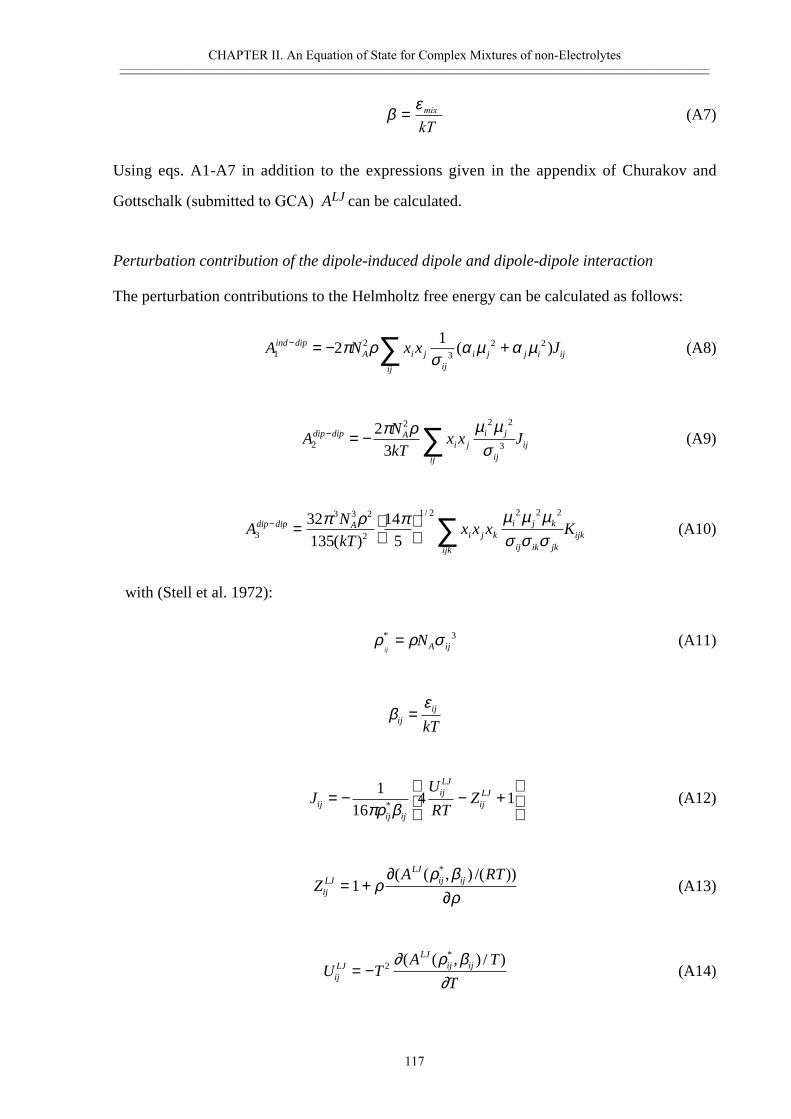
CHAPTER II. An Equation of State for Complex Mixtures of non-Electrolytes————————————————————————————————————————————————————————
117
kTmixεβ = (A7)
Using eqs. A1-A7 in addition to the expressions given in the appendix of Churakov and
Gottschalk (submitted to GCA) ALJ can be calculated.
Perturbation contribution of the dipole-induced dipole and dipole-dipole interaction
The perturbation contributions to the Helmholtz free energy can be calculated as follows:
A N x x Jind dipA i j
iji j j i
ij
ij12
32 22
1− = − +∑π ρσ
α µ α µ( ) (A8)
AN
kTx x Jdip dip A
i ji j
ijij
ij2
2 2 2
3
23
− = − ∑π ρ µ µσ
(A9)
AN
kTx x x Kdip dip A
i j ki j k
ij ik jkijk
ijk3
3 3 2
2
1 2 2 2 232135
145
− =
∑π ρ π µ µ µ
σ σ σ( )
/
(A10)
with (Stell et al. 1972):
ρ ρ σij
NA ij* = 3 (A11)
βε
ijij
kT=
JU
RTZij
ij ij
ijLJ
ijLJ= − − +
116
4 1πρ β* (A12)
ZA RT
ijLJ
LJij ij= +
∂∂
1 ρρ β
ρ( ( , ) /( ))*
(A13)
U TA T
TijLJ
LJij ij= − 2 ∂ ρ β
∂( ( , ) / )*
(A14)
CHAPTER II. An Equation of State for Complex Mixtures of non-Electrolytes————————————————————————————————————————————————————————
118
K K K Kijk ij ij ik ik jk jk= [ ]( , ) ( , ) ( , )* * * /ρ β ρ β ρ β
1 3(A15)
ln ( , ) ( ) ( ) ( )* * * * *K Ln Ln Lnij ij ij ij ij ij ij ij ijρ β ρ β ρ ρ β ρ β[ ] = − + − + − +M M M M M M 1 2 3 4 5 6
2 2(A16)
The coefficients M1 to M6 are identical to those for pure fluids (Churakov and Gottschalksubmitted to GCA).

Size and Topology of Molecular Clusters in Supercritical Water:
a Molecular Dynamics Simulation
CCHHAAPPTTEERR IIIIII.. TThheerrmmooddyynnaammiiccss aanndd SSttrruuccttuurree ooff SSuuppeerrccrriittiiccaall WWaatteerr————————————————————————————————————————————————————————————————————————————————————————————————————————————————
120
Abstract
A hybrid criterion of hydrogen bonding is applied to the analysis of molecular
dynamics trajectories simulated for several near- and supercritical thermodynamic conditions.
Even at vapor-like densities supercritical water is shown to contain large molecular clusters,
consisting of up to 10 molecules. Relative abundances of topologically different trimers,
tetramers, and pentamers are examined, and chain-like clusters are found predominant under
supercritical conditions. In contrast to the results of quantum-chemical calculations for
isolated water clusters, ring-like clusters are only rarely formed in supercritical water.

CCHHAAPPTTEERR IIIIII.. TThheerrmmooddyynnaammiiccss aanndd SSttrruuccttuurree ooff SSuuppeerrccrriittiiccaall WWaatteerr————————————————————————————————————————————————————————————————————————————————————————————————————————————————
121
1. Introduction
In the near-critical region the properties of any fluid change dramatically over a
relatively narrow range of temperatures and pressures [1]. These changes also affect the fluid
structure. The structure of liquid water is known to be dominated by the formation of
hydrogen bonds connecting all water molecules. However, the very persistence of hydrogen
bonding up to the critical point of water (Tc = 647 K = 374°C; Pc = 22.1 MPa; ρc = 0.32
g/cm3) has been a matter of significant controversy until recently [2–17].
It is now well established both experimentally [10,13–15] and by molecular computer
simulations [3–9,11,12,16,17] that H-bonds in water do persist even above the critical
temperature. Although the infinite percolating network of H-bonds breaks apart with the
increase of temperature, individual molecules in supercritical water for significant amount of
time remain bonded in smaller molecular aggregates, or clusters [16]. Quantitative
understanding of the size and structure of such clusters is important for many fundamental
and practical reasons. For example, recent estimations suggest that large pressure effects on
the isotope fractionation between high-temperature aqueous solutions and minerals can be
explained by taking into account the degree of clusterization in water vapor [18].
A hybrid criterion of H-bonding based on molecular distance–energy distribution
functions has already been applied to the analysis of molecular configurations generated by
Monte Carlo computer simulations over wide ranges of temperature and pressure [5,16] and
has shown to give quantitative results consistent with all available experimental data [10,13–
15]. In this Letter we apply the same criterion to the analysis of molecular dynamics
trajectories simulated for several near- and supercritical thermodynamic conditions. Based on
this analysis we calculate size and shape distributions of molecular clusters in supercritical
water, and examine topological and structural characteristics of the most common clusters,
such as trimers, tetramers, and pentamers.
2. Molecular dynamics simulations
The MD simulations were performed using a conventional molecular dynamics
algorithm for the canonical (NVE) ensemble [19]. The systems studied consisted of 200 water
molecules in a cubic box with periodic boundary conditions. The side length of the simulation
box was adjusted from run to run to give the required density in the range between 0.17 and
1.28 g/cm3 which corresponded to the pressure range of 25 MPa < P < 3000 MPa. Five
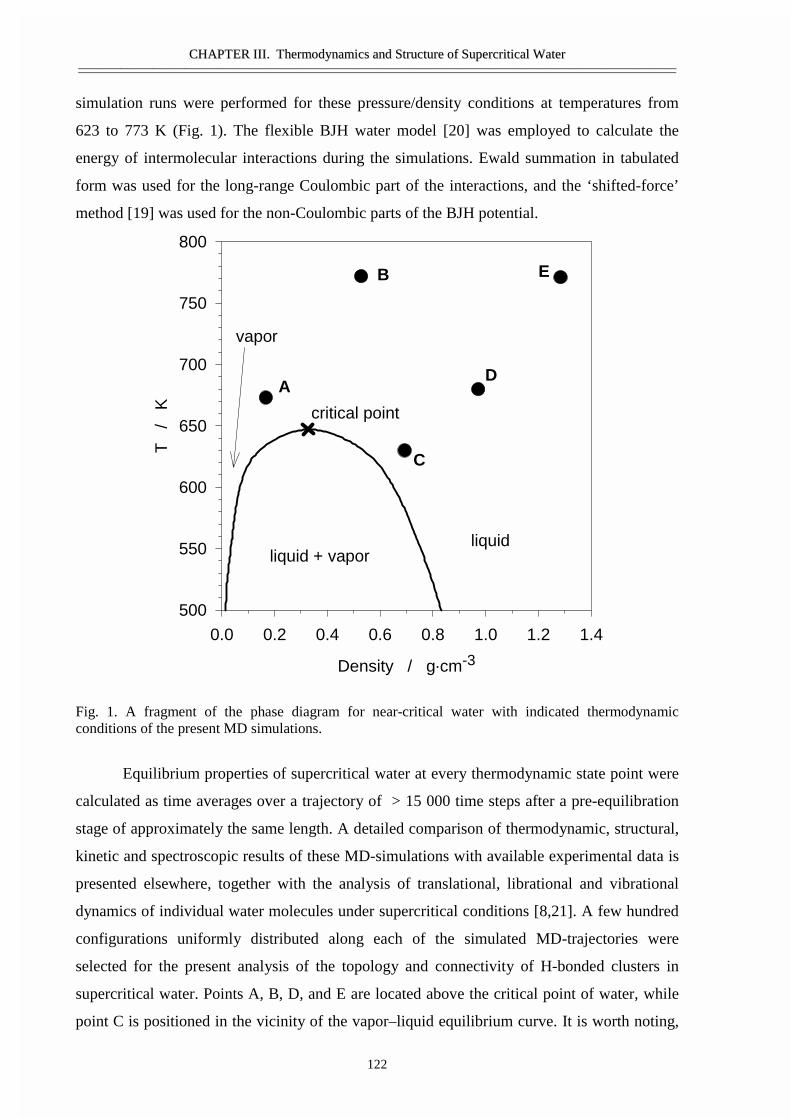
CCHHAAPPTTEERR IIIIII.. TThheerrmmooddyynnaammiiccss aanndd SSttrruuccttuurree ooff SSuuppeerrccrriittiiccaall WWaatteerr————————————————————————————————————————————————————————————————————————————————————————————————————————————————
122
simulation runs were performed for these pressure/density conditions at temperatures from
623 to 773 K (Fig. 1). The flexible BJH water model [20] was employed to calculate the
energy of intermolecular interactions during the simulations. Ewald summation in tabulated
form was used for the long-range Coulombic part of the interactions, and the ‘shifted-force’
method [19] was used for the non-Coulombic parts of the BJH potential.
Fig. 1. A fragment of the phase diagram for near-critical water with indicated thermodynamicconditions of the present MD simulations.
Equilibrium properties of supercritical water at every thermodynamic state point were
calculated as time averages over a trajectory of > 15 000 time steps after a pre-equilibration
stage of approximately the same length. A detailed comparison of thermodynamic, structural,
kinetic and spectroscopic results of these MD-simulations with available experimental data is
presented elsewhere, together with the analysis of translational, librational and vibrational
dynamics of individual water molecules under supercritical conditions [8,21]. A few hundred
configurations uniformly distributed along each of the simulated MD-trajectories were
selected for the present analysis of the topology and connectivity of H-bonded clusters in
supercritical water. Points A, B, D, and E are located above the critical point of water, while
point C is positioned in the vicinity of the vapor–liquid equilibrium curve. It is worth noting,
Density / g.cm-3
0.0 0.2 0.4 0.6 0.8 1.0 1.2 1.4
T
/ K
500
550
600
650
700
750
800
A
B
C
D
E
liquidliquid + vapor
vapor
critical point
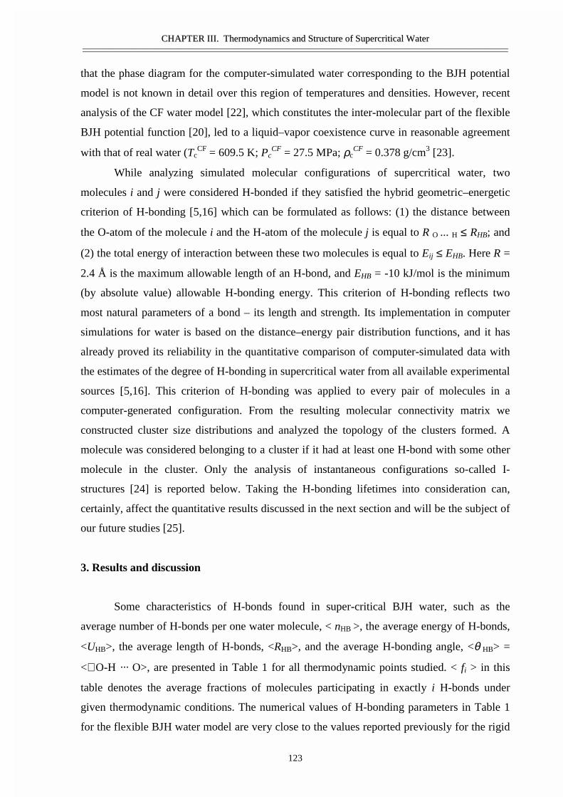
CCHHAAPPTTEERR IIIIII.. TThheerrmmooddyynnaammiiccss aanndd SSttrruuccttuurree ooff SSuuppeerrccrriittiiccaall WWaatteerr————————————————————————————————————————————————————————————————————————————————————————————————————————————————
123
that the phase diagram for the computer-simulated water corresponding to the BJH potential
model is not known in detail over this region of temperatures and densities. However, recent
analysis of the CF water model [22], which constitutes the inter-molecular part of the flexible
BJH potential function [20], led to a liquid–vapor coexistence curve in reasonable agreement
with that of real water (TcCF = 609.5 K; Pc
CF = 27.5 MPa; ρcCF = 0.378 g/cm3 [23].
While analyzing simulated molecular configurations of supercritical water, two
molecules i and j were considered H-bonded if they satisfied the hybrid geometric–energetic
criterion of H-bonding [5,16] which can be formulated as follows: (1) the distance between
the O-atom of the molecule i and the H-atom of the molecule j is equal to R O ... H ≤ RHB; and
(2) the total energy of interaction between these two molecules is equal to Eij ≤ EHB. Here R =
2.4 Å is the maximum allowable length of an H-bond, and EHB = -10 kJ/mol is the minimum
(by absolute value) allowable H-bonding energy. This criterion of H-bonding reflects two
most natural parameters of a bond – its length and strength. Its implementation in computer
simulations for water is based on the distance–energy pair distribution functions, and it has
already proved its reliability in the quantitative comparison of computer-simulated data with
the estimates of the degree of H-bonding in supercritical water from all available experimental
sources [5,16]. This criterion of H-bonding was applied to every pair of molecules in a
computer-generated configuration. From the resulting molecular connectivity matrix we
constructed cluster size distributions and analyzed the topology of the clusters formed. A
molecule was considered belonging to a cluster if it had at least one H-bond with some other
molecule in the cluster. Only the analysis of instantaneous configurations so-called I-
structures [24] is reported below. Taking the H-bonding lifetimes into consideration can,
certainly, affect the quantitative results discussed in the next section and will be the subject of
our future studies [25].
3. Results and discussion
Some characteristics of H-bonds found in super-critical BJH water, such as the
average number of H-bonds per one water molecule, < nHB >, the average energy of H-bonds,
<UHB>, the average length of H-bonds, <RHB>, and the average H-bonding angle, <θ HB> =
<∠ O-H ··· O>, are presented in Table 1 for all thermodynamic points studied. < fi > in this
table denotes the average fractions of molecules participating in exactly i H-bonds under
given thermodynamic conditions. The numerical values of H-bonding parameters in Table 1
for the flexible BJH water model are very close to the values reported previously for the rigid
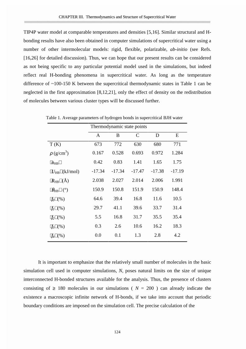
CCHHAAPPTTEERR IIIIII.. TThheerrmmooddyynnaammiiccss aanndd SSttrruuccttuurree ooff SSuuppeerrccrriittiiccaall WWaatteerr————————————————————————————————————————————————————————————————————————————————————————————————————————————————
124
TIP4P water model at comparable temperatures and densities [5,16]. Similar structural and H-
bonding results have also been obtained in computer simulations of supercritical water using a
number of other intermolecular models: rigid, flexible, polarizable, ab-initio (see Refs.
[16,26] for detailed discussion). Thus, we can hope that our present results can be considered
as not being specific to any particular potential model used in the simulations, but indeed
reflect real H-bonding phenomena in supercritical water. As long as the temperature
difference of ~100-150 K between the supercritical thermodynamic states in Table 1 can be
neglected in the first approximation [8,12,21], only the effect of density on the redistribution
of molecules between various cluster types will be discussed further.
Table 1. Average parameters of hydrogen bonds in supercritical BJH water
Thermodynamic state points
A B C D E
T (K) 673 772 630 680 771
ρ (g/cm3) 0.167 0.528 0.693 0.972 1.284
⟨nHB⟩ 0.42 0.83 1.41 1.65 1.75
⟨UHB⟩ (kJ/mol) -17.34 -17.34 -17.47 -17.38 -17.19
⟨RHB⟩ (Å) 2.038 2.027 2.014 2.006 1.991
⟨θHB⟩ (°) 150.9 150.8 151.9 150.9 148.4
⟨ f0⟩ (%) 64.6 39.4 16.8 11.6 10.5
⟨ f1⟩ (%) 29.7 41.1 39.6 33.7 31.4
⟨ f2⟩ (%) 5.5 16.8 31.7 35.5 35.4
⟨ f3⟩ (%) 0.3 2.6 10.6 16.2 18.3
⟨ f4⟩ (%) 0.0 0.1 1.3 2.8 4.2
It is important to emphasize that the relatively small number of molecules in the basic
simulation cell used in computer simulations, N, poses natural limits on the size of unique
interconnected H-bonded structures available for the analysis. Thus, the presence of clusters
consisting of ≥ 180 molecules in our simulations ( N = 200 ) can already indicate the
existence a macroscopic infinite network of H-bonds, if we take into account that periodic
boundary conditions are imposed on the simulation cell. The precise calculation of the
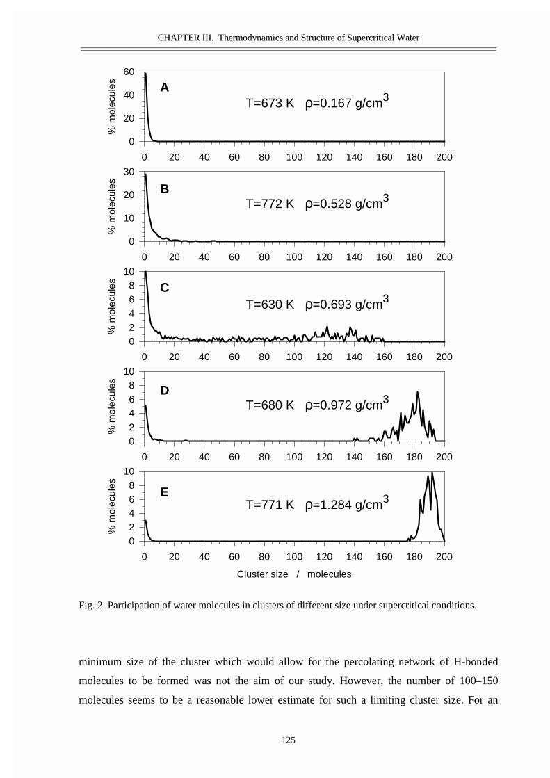
CCHHAAPPTTEERR IIIIII.. TThheerrmmooddyynnaammiiccss aanndd SSttrruuccttuurree ooff SSuuppeerrccrriittiiccaall WWaatteerr————————————————————————————————————————————————————————————————————————————————————————————————————————————————
125
Fig. 2. Participation of water molecules in clusters of different size under supercritical conditions.
minimum size of the cluster which would allow for the percolating network of H-bonded
molecules to be formed was not the aim of our study. However, the number of 100–150
molecules seems to be a reasonable lower estimate for such a limiting cluster size. For an
0 20 40 60 80 100 120 140 160 180 200
% m
olec
ules
0
20
40
60
0 20 40 60 80 100 120 140 160 180 200
% m
olec
ules
0
10
20
30
0 20 40 60 80 100 120 140 160 180 200
% m
olec
ules
02468
10
0 20 40 60 80 100 120 140 160 180 200
% m
olec
ules
02468
10
Cluster size / molecules
0 20 40 60 80 100 120 140 160 180 200
% m
olec
ules
02468
10
T=673 K ρ=0.167 g/cm3
T=772 K ρ=0.528 g/cm3
T=630 K ρ=0.693 g/cm3
T=680 K ρ=0.972 g/cm3
T=771 K ρ=1.284 g/cm3
A
B
C
D
E
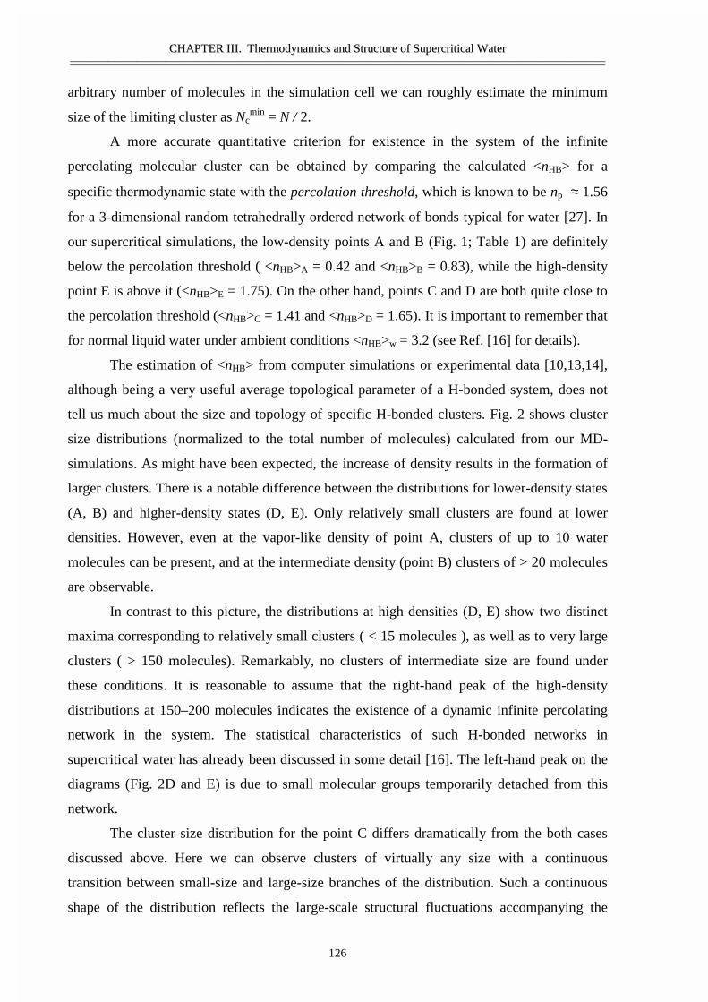
CCHHAAPPTTEERR IIIIII.. TThheerrmmooddyynnaammiiccss aanndd SSttrruuccttuurree ooff SSuuppeerrccrriittiiccaall WWaatteerr————————————————————————————————————————————————————————————————————————————————————————————————————————————————
126
arbitrary number of molecules in the simulation cell we can roughly estimate the minimum
size of the limiting cluster as Ncmin = N / 2.
A more accurate quantitative criterion for existence in the system of the infinite
percolating molecular cluster can be obtained by comparing the calculated <nHB> for a
specific thermodynamic state with the percolation threshold, which is known to be np ≈ 1.56
for a 3-dimensional random tetrahedrally ordered network of bonds typical for water [27]. In
our supercritical simulations, the low-density points A and B (Fig. 1; Table 1) are definitely
below the percolation threshold ( <nHB>A = 0.42 and <nHB>B = 0.83), while the high-density
point E is above it (<nHB>E = 1.75). On the other hand, points C and D are both quite close to
the percolation threshold (<nHB>C = 1.41 and <nHB>D = 1.65). It is important to remember that
for normal liquid water under ambient conditions <nHB>w = 3.2 (see Ref. [16] for details).
The estimation of <nHB> from computer simulations or experimental data [10,13,14],
although being a very useful average topological parameter of a H-bonded system, does not
tell us much about the size and topology of specific H-bonded clusters. Fig. 2 shows cluster
size distributions (normalized to the total number of molecules) calculated from our MD-
simulations. As might have been expected, the increase of density results in the formation of
larger clusters. There is a notable difference between the distributions for lower-density states
(A, B) and higher-density states (D, E). Only relatively small clusters are found at lower
densities. However, even at the vapor-like density of point A, clusters of up to 10 water
molecules can be present, and at the intermediate density (point B) clusters of > 20 molecules
are observable.
In contrast to this picture, the distributions at high densities (D, E) show two distinct
maxima corresponding to relatively small clusters ( < 15 molecules ), as well as to very large
clusters ( > 150 molecules). Remarkably, no clusters of intermediate size are found under
these conditions. It is reasonable to assume that the right-hand peak of the high-density
distributions at 150–200 molecules indicates the existence of a dynamic infinite percolating
network in the system. The statistical characteristics of such H-bonded networks in
supercritical water has already been discussed in some detail [16]. The left-hand peak on the
diagrams (Fig. 2D and E) is due to small molecular groups temporarily detached from this
network.
The cluster size distribution for the point C differs dramatically from the both cases
discussed above. Here we can observe clusters of virtually any size with a continuous
transition between small-size and large-size branches of the distribution. Such a continuous
shape of the distribution reflects the large-scale structural fluctuations accompanying the
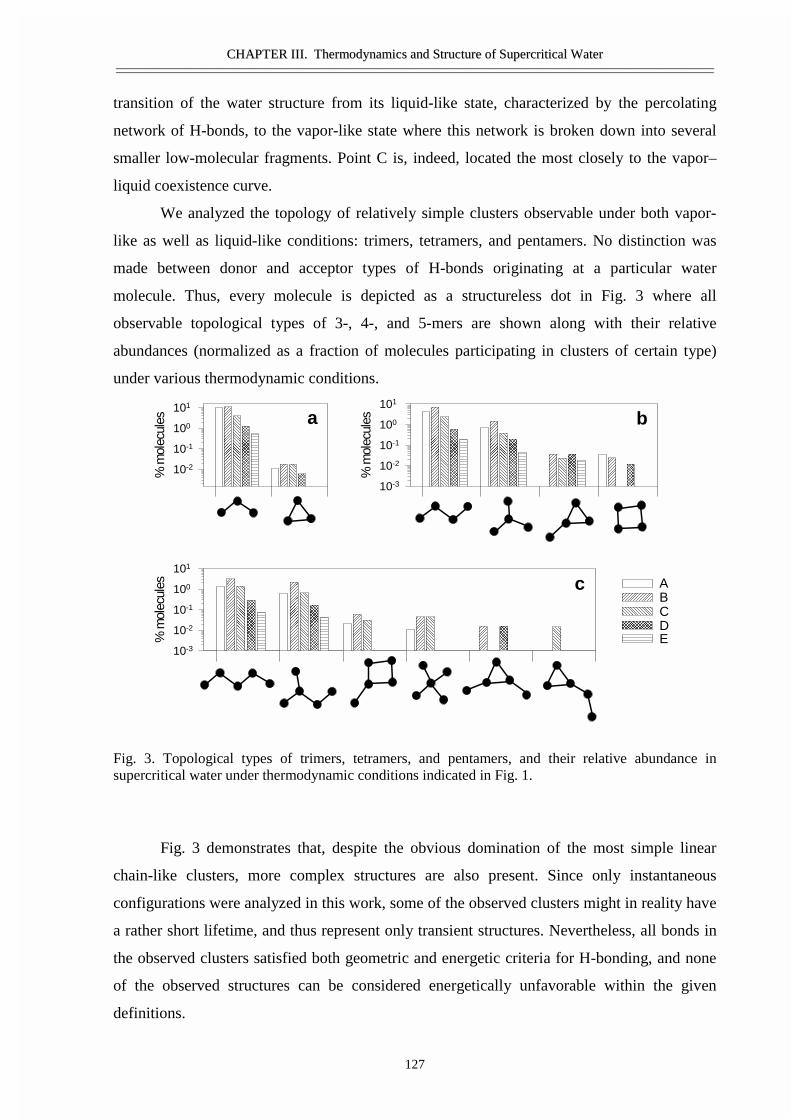
CCHHAAPPTTEERR IIIIII.. TThheerrmmooddyynnaammiiccss aanndd SSttrruuccttuurree ooff SSuuppeerrccrriittiiccaall WWaatteerr————————————————————————————————————————————————————————————————————————————————————————————————————————————————
127
transition of the water structure from its liquid-like state, characterized by the percolating
network of H-bonds, to the vapor-like state where this network is broken down into several
smaller low-molecular fragments. Point C is, indeed, located the most closely to the vapor–
liquid coexistence curve.
We analyzed the topology of relatively simple clusters observable under both vapor-
like as well as liquid-like conditions: trimers, tetramers, and pentamers. No distinction was
made between donor and acceptor types of H-bonds originating at a particular water
molecule. Thus, every molecule is depicted as a structureless dot in Fig. 3 where all
observable topological types of 3-, 4-, and 5-mers are shown along with their relative
abundances (normalized as a fraction of molecules participating in clusters of certain type)
under various thermodynamic conditions.
Fig. 3. Topological types of trimers, tetramers, and pentamers, and their relative abundance insupercritical water under thermodynamic conditions indicated in Fig. 1.
Fig. 3 demonstrates that, despite the obvious domination of the most simple linear
chain-like clusters, more complex structures are also present. Since only instantaneous
configurations were analyzed in this work, some of the observed clusters might in reality have
a rather short lifetime, and thus represent only transient structures. Nevertheless, all bonds in
the observed clusters satisfied both geometric and energetic criteria for H-bonding, and none
of the observed structures can be considered energetically unfavorable within the given
definitions.
% m
olec
ules
10-2
10-1
100
101
% m
olec
ules
10-3
10-2
10-1
100
101
% m
olec
ules
10-3
10-2
10-1
100
101
ABCDE
a b
c
CCHHAAPPTTEERR IIIIII.. TThheerrmmooddyynnaammiiccss aanndd SSttrruuccttuurree ooff SSuuppeerrccrriittiiccaall WWaatteerr————————————————————————————————————————————————————————————————————————————————————————————————————————————————
128
Only two topological types are possible for trimers: a chain and a 3-member ring. As
seen in Fig. 3a, > 99% of all trimers are present in the form of linear chains under
supercritical conditions. This is, of course, not surprising, since the formation of a 3-member
ring can only be possible by significant bending of all three H-bonds, thus making this
structure energetically less favorable.
Four water molecules can theoretically form 6 topologically different types of
tetramers, 4 of which were observed in our simulations. Fig. 3b shows that the most abundant
tetramers have chain-like structure (1) under all thermodynamic conditions studied. Such
linear structures constitute >80% of all tetramers, while another 17% are represented by an
open structure (2), which can be described as a branched chain. Configurations containing 3-
or 4- member rings constitute in total < 3% of all tetramers.
Five water molecules can form 14 topologically different types of pentamers. Some of
them are, obviously, energetically unfavorable and never materialize. In supercritical water
we have found only 6 topological types of pentamers shown in Fig. 3c. Once again, the
simplest linear chain-like cluster (1) is the most abundant type and constitutes ~ 63% of all
pentamers. Almost twice less abundant (35% of pentamers) are slightly branched linear
clusters (2). The remaining four types observed in the simulations constitute together ~2%,
and poor statistics prevents us to analyze the density dependence of their relative abundances.
It is interesting to note that present results on the topology of H-bonded molecular
clusters in supercritical water significantly differ from the results of quantum-chemical
calculations which consistently identify ring-like cluster structures as the most stable ones
(see e.g. Ref. 28). Five-member rings were not found in our simulations even as less abundant
species, while the presence of 3- and 4-member rings is very small. This contradiction can be
explained by the fundamental difference in the thermodynamic conditions of these two types
of calculations. Under high supercritical temperatures of our simulations, ring-like structures
are becoming unstable because of the high kinetic energy of the constituting water molecules.
This can also be confirmed by the molecular dynamics simulations of isolated pentamers
[29,30], where 5-member rings have been found at the limit of their stability even at near-
ambient temperatures.
Almost total absence of pentamers organized in complete tetrahedral clusters (4 in Fig.
3c) is also remarkable, since tetrahedral local ordering is the most distinct feature of H-
bonded networks in water. Furthermore, the experimental data on X-ray diffraction is
supercritical water [10,31] show a peak of molecular distribution function corresponding to
tetrahedrally-ordered second-nearest neighbors exactly under the thermodynamic conditions
CCHHAAPPTTEERR IIIIII.. TThheerrmmooddyynnaammiiccss aanndd SSttrruuccttuurree ooff SSuuppeerrccrriittiiccaall WWaatteerr————————————————————————————————————————————————————————————————————————————————————————————————————————————————
129
of point B of the present study. This apparent contradiction is easily resolved if we note that
tetrahedrally-coordinated second-neighboring molecules can be found in any of the observed
clusters starting from trimers. Therefore, all these clusters, and not just full tetrahedra, can
represent the fragments of a larger tetrahedrally-coordinated H-bonded network. Similar to
the ring-like structures, such pentamers are, obviously, less stable at supercritical
temperatures.
4. Conclusions
Our analysis of MD simulation results for supercritical water using the hybrid
geometric and energetic criterion of hydrogen bonding [5,16] demonstrates that even low-
density water vapor (ρ < 0.2 g/cm3) under supercritical conditions can contain quite large
molecular clusters, consisting of up to 10 molecules. No significant density dependence of
relative abundances for topologically different water clusters of small size is observed, and
chain-like clusters are found predominant under supercritical conditions. In contrast to the
results of quantum-chemical calculations for isolated water clusters which identify ring-like
structures as the most stable energetically, such structures are only rarely formed under
supercritical conditions. Somewhat counterintuitively, the fraction of pentamers topologically
organized as complete tetrahedra is also insignificant under these conditions.
Acknowledgements
The work has been supported by INTAS (Grants UA-95-0096 and 96-1989), CRDF
(Grant RC1-170), and the Russian Foundation for Basic Research (Grant 95-03-32587). The
authors are grateful to Yu.E. Gorbaty for permanent interest in this work and useful
discussions, and to A.A. Chialvo and P.T. Cummings for kindly providing the manuscript of
their review paper prior to publication.
References
1. R.W. Shaw, T.B. Brill, A.A. Clifford, C.A. Eckert, E.U. Franck, Chem. Eng. News 69(51)
(1990) 26.
2. P. Postorino, R.H. Tromp, M.A. Ricci, A.K. Soper, G.W. Neilson, Nature (London) 366
(1993) 668
CCHHAAPPTTEERR IIIIII.. TThheerrmmooddyynnaammiiccss aanndd SSttrruuccttuurree ooff SSuuppeerrccrriittiiccaall WWaatteerr————————————————————————————————————————————————————————————————————————————————————————————————————————————————
130
3. A. Chialvo, P.T. Cummings, J. Chem. Phys. 101 (1994) 4466.
4. E.S. Fois, M. Sprik, M. Parrinello, Chem. Phys. Lett. 223 (1994) 411.
5. A.G. Kalinichev, J.D. Bass, Chem. Phys. Lett. 231 (1994) 301.
6. T.I. Mizan, P.E. Savage, R.M. Ziff, J. Phys. Chem. 98 (1994) 13067.
7. G. Loffler, H. Schreiber, O. Steinhauser, Ber. Bunsenges. Phys. Chem. 98 (1994) 1575.
8. A.G. Kalinichev, K. Heinzinger, Geochim. Cosmochim. Acta 59 (1995) 641.
9. R.D. Mountain, J. Chem. Phys. 103 (1995) 3084.
10. Yu.E. Gorbaty, A.G. Kalinichev, J. Phys. Chem. 99 (1995) 5336.
11. A. Chialvo, P.T. Cummings, J. Phys. Chem. 100 (1996) 1309.
12. T.I. Mizan, P.E. Savage, R.M. Ziff, J. Phys. Chem. 100 (1996) 403.
13. M.M. Hoffmann, M.S. Conradi, J. Am. Chem. Soc. 119 (1997) 3811.
14. A.K. Soper, F. Bruni, M.A. Ricci, J. Chem. Phys. 106 (1997) 247.
15. N. Matubayasi, C. Wakai, M. Nakahara, J. Chem. Phys. 107 (1997) 9133.
16. A.G. Kalinichev, J.D. Bass, J. Phys. Chem. A 101 (1997) 9720.
17. P. Jedlovszky, J.P. Brodholt, F. Bruni, M.A. Ricci, A.K. Soper, R. Vallauri, J. Chem.
Phys. 108 (1998) 8528.
18. T. Driesner, Science 277 (1997) 791.
19. M.P. Allen, D.J. Tildesley, Computer Simulation of Liquids, Oxford University Press,
New York, 1987.
20. P. Bopp, G. Jancso, K. Heinzinger, Chem. Phys. Lett. 98 (1983) 129.
21. A.G. Kalinichev, Ber. Bunsenges. Phys. Chem. 97 (1993) 872.
22. F.H. Stillinger, A. Rahman, J. Chem. Phys. 68 (1978) 666.
23. B. Guillot, Y. Guissani, J. Chem. Phys. 108 (1998) 10162.
24. D. Eisenberg, W. Kautzmann, The Structure and Properties of Water, Oxford University
Press, Oxford, 1969.
25. A.G. Kalinichev, S.V. Churakov in preparation
26. A.A. Chialvo, P.T. Cummings, Adv. Chem. Phys. (1999), in. print.
27. H.E. Stanley, J. Teixeira, J. Chem. Phys. 73 (1980) 3404.
28. J.K. Gregory, D.C. Clary, J. Phys. Chem. 100 (1996) 18014.
29. P.L.M. Plummer, T.S. Chen, J. Chem. Phys. 86 (1987) 7149.
30. W.B. Bosma, L.E. Fried, S. Mukamel, J. Chem. Phys. 98 (1993) 4413.
31. Yu.E. Gorbaty, Yu.N. Demianets, Chem. Phys. Lett. 100 (1983) 450.
Size, Structure and Abundance of Molecular Clusters
in Supercritical Water Over Wide Range of Densities:
Monte Carlo Simulations
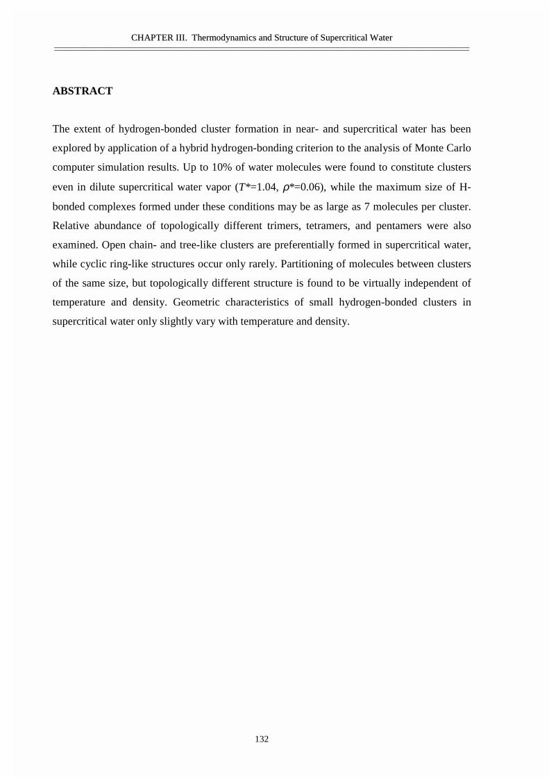
CCHHAAPPTTEERR IIIIII.. TThheerrmmooddyynnaammiiccss aanndd SSttrruuccttuurree ooff SSuuppeerrccrriittiiccaall WWaatteerr————————————————————————————————————————————————————————————————————————————————————————————————————————————————
132
ABSTRACT
The extent of hydrogen-bonded cluster formation in near- and supercritical water has been
explored by application of a hybrid hydrogen-bonding criterion to the analysis of Monte Carlo
computer simulation results. Up to 10% of water molecules were found to constitute clusters
even in dilute supercritical water vapor (T*=1.04, ρ*=0.06), while the maximum size of H-
bonded complexes formed under these conditions may be as large as 7 molecules per cluster.
Relative abundance of topologically different trimers, tetramers, and pentamers were also
examined. Open chain- and tree-like clusters are preferentially formed in supercritical water,
while cyclic ring-like structures occur only rarely. Partitioning of molecules between clusters
of the same size, but topologically different structure is found to be virtually independent of
temperature and density. Geometric characteristics of small hydrogen-bonded clusters in
supercritical water only slightly vary with temperature and density.
CCHHAAPPTTEERR IIIIII.. TThheerrmmooddyynnaammiiccss aanndd SSttrruuccttuurree ooff SSuuppeerrccrriittiiccaall WWaatteerr————————————————————————————————————————————————————————————————————————————————————————————————————————————————
133
INTRODUCTION
Over the last several years, significant efforts have been made to examine the structure of
supercritical water using both experimental methods and computer simulations [1-19]. More
recently, the formation of small molecular clusters in high temperature water vapor, as well as
in supercritical fluid has attracted particular attention [18,20,21]. The nucleation of clusters
results in local structural and density heterogeneity in the fluid. In different clusters water
molecules possess slightly different properties such as the dipole moment and lengths of
interatomic bonds [9]. So, topologically different water complexes may be even considered as
distinct chemical compounds. Quantitative understanding of the size and structure of such
clusters is important for many fundamental and practical reasons. For example, recent
calculations suggest that the large effects of pressure on the isotope fractionation between
high temperature aqueous solutions and minerals can be explained by taking into account the
degree of clusterization in water vapor [21].
We applied Monte Carlo computer simulations to investigate the statistics of size and
topology distributions of hydrogen-bonded water clusters over wide ranges of near- and
supercritical temperatures and densities. Particular emphasis has been made on the geometry
of the most abundant trimers, tetramers, and pentamers of water molecules.
METHOD OF MODELING
The simulations were performed using a conventional Monte Carlo algorithm for the
isothermal-isobaric (NPT) ensemble [22]. The investigated systems consisted of 216 water
molecules interacting via the TIP4P [23] rigid four site effective pair potential in the cubic
box with periodic boundary conditions. About 50 million MC steps were performed for each
of the ~40 thermodynamic points studied, and about 5000 equilibrium statistically
independent molecular configurations (separated by 10000 MC steps) were accumulated at
every thermodynamic point for further analysis of the structure of hydrogen-bonded network.
Other specific details of the simulation technique are reported elsewhere [13,19,20].
While analyzing the simulated molecular configurations of supercritical water, two molecules
i and j were considered hydrogen-bonded if they satisfied the hybrid geometric-energetic
CCHHAAPPTTEERR IIIIII.. TThheerrmmooddyynnaammiiccss aanndd SSttrruuccttuurree ooff SSuuppeerrccrriittiiccaall WWaatteerr————————————————————————————————————————————————————————————————————————————————————————————————————————————————
134
criterion of H-bonding [13,19] which can be formulated as follows: (1) the distance between
the O-atom of the molecule i and the H-atom of the molecule j is equal to RO...H ≤ RHB, and
(2) the total energy of interaction between these two molecules is equal to Eij ≤ EHB. Here
RHB = 2.4 Å is the maximum allowable length of a hydrogen bond, and EHB = –10 kJ/mol is
the minimum (by absolute value) allowable H-bonding energy. This criterion of H-bonding is
directly related to the two most natural parameters of a bond — its length and strength. The
implementation of this criterion in computer simulations for water is based on the distance-
energy pair distribution functions, and it has already proved its reliability in the quantitative
comparison of computer-simulated data with the estimates of the degree of hydrogen bonding
in supercritical water from all available experimental sources [13, 19]. This criterion of H-
bonding was applied to every pair of molecules in a computer-generated configuration. From
the resulting connectivity matrix, the groups of molecules interconnected by a network of H-
bonds were collected to obtain cluster size distributions. By indexing the interconnected
molecules, geometric and energetic characteristics of each isolated cluster were obtained. A
molecule was considered belonging to a cluster if it had at least one H-bond with some other
molecule in the cluster. Following this method, the maximum cluster size is limited by the
total number of molecules in the simulation box (216 in the current study). Molecules were
considered to form an infinite percolating H-bonded network, if a periodic image of at least
one of them belonged to the same cluster as it’s origin. Due to the time-independent nature of
the Monte Carlo simulations, only the analysis of instantaneous configurations (so called I-
structures [24]) is reported here. Taking the H-bonding lifetimes into consideration can,
certainly, affect the quantitative results discussed below (e.g., [18]) and will be the subject of
our future molecular dynamics simulations.
RESULTS AND DISCUSSION
While accurately predicting the structure and volumetric properties of liquid water [23], the
TIP4P potential has critical parameters slightly shifted with respect to the experimental data
[25]. However, our goal was not the most accurate prediction of the volumetric properties, but
rather the detailed quantitative analysis of the structure of fluid water at varying pressures,
temperatures, and densities. The discrepancies between simulated and experimental properties
of water can be accounted for by an appropriate choice of the critical parameters. Following
the method of Guissani and Guillot [26], the equation of state[27]:
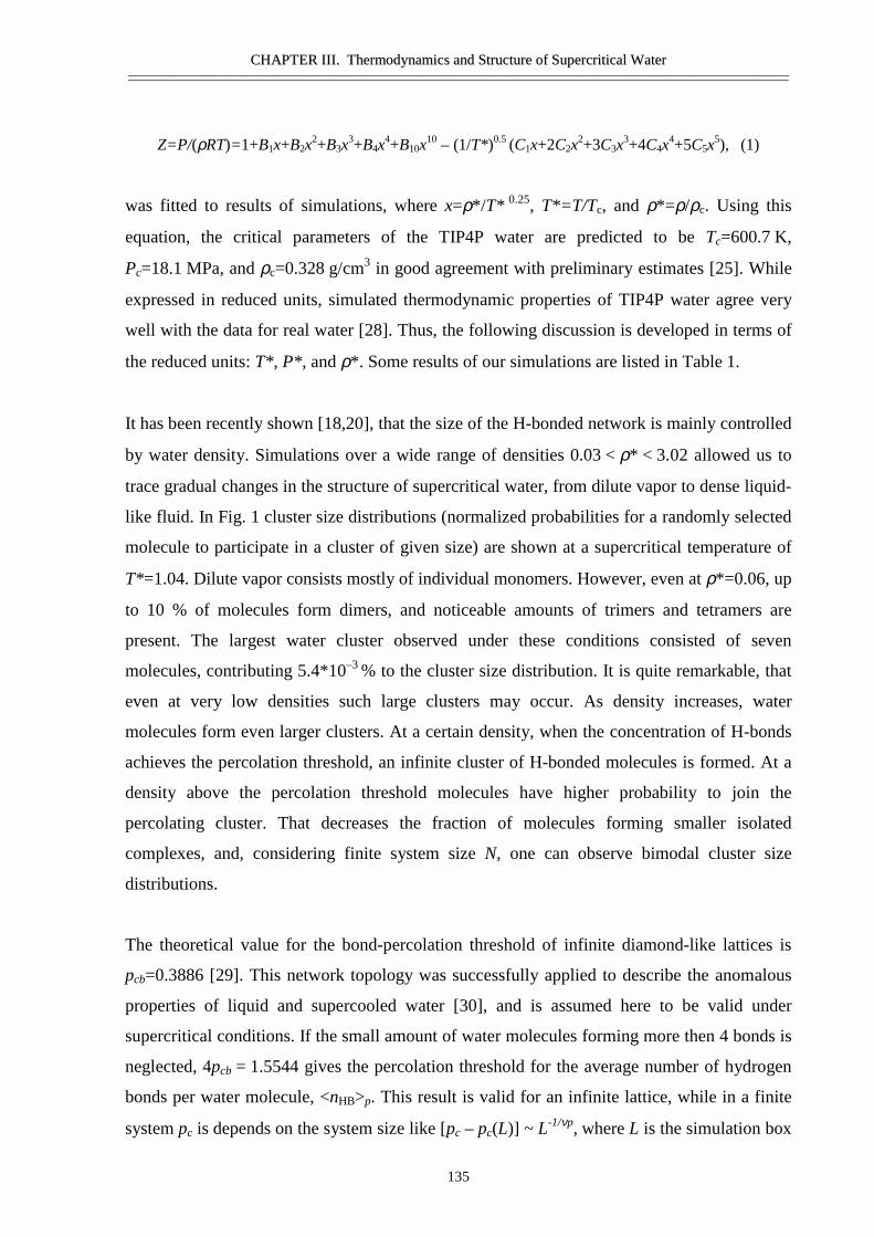
CCHHAAPPTTEERR IIIIII.. TThheerrmmooddyynnaammiiccss aanndd SSttrruuccttuurree ooff SSuuppeerrccrriittiiccaall WWaatteerr————————————————————————————————————————————————————————————————————————————————————————————————————————————————
135
Z=P/(ρRT)=1+B1x+B2x2+B3x
3+B4x4+B10x
10 – (1/T*)0.5 (C1x+2C2x2+3C3x
3+4C4x4+5C5x
5), (1)
was fitted to results of simulations, where x=ρ*/T* 0.25, T*=T/Tc, and ρ*=ρ/ρc. Using this
equation, the critical parameters of the TIP4P water are predicted to be Tc=600.7 K,
Pc=18.1 MPa, and ρc=0.328 g/cm3 in good agreement with preliminary estimates [25]. While
expressed in reduced units, simulated thermodynamic properties of TIP4P water agree very
well with the data for real water [28]. Thus, the following discussion is developed in terms of
the reduced units: T*, P*, and ρ*. Some results of our simulations are listed in Table 1.
It has been recently shown [18,20], that the size of the H-bonded network is mainly controlled
by water density. Simulations over a wide range of densities 0.03 < ρ* < 3.02 allowed us to
trace gradual changes in the structure of supercritical water, from dilute vapor to dense liquid-
like fluid. In Fig. 1 cluster size distributions (normalized probabilities for a randomly selected
molecule to participate in a cluster of given size) are shown at a supercritical temperature of
T*=1.04. Dilute vapor consists mostly of individual monomers. However, even at ρ*=0.06, up
to 10 % of molecules form dimers, and noticeable amounts of trimers and tetramers are
present. The largest water cluster observed under these conditions consisted of seven
molecules, contributing 5.4*10–3 % to the cluster size distribution. It is quite remarkable, that
even at very low densities such large clusters may occur. As density increases, water
molecules form even larger clusters. At a certain density, when the concentration of H-bonds
achieves the percolation threshold, an infinite cluster of H-bonded molecules is formed. At a
density above the percolation threshold molecules have higher probability to join the
percolating cluster. That decreases the fraction of molecules forming smaller isolated
complexes, and, considering finite system size N, one can observe bimodal cluster size
distributions.
The theoretical value for the bond-percolation threshold of infinite diamond-like lattices is
pcb=0.3886 [29]. This network topology was successfully applied to describe the anomalous
properties of liquid and supercooled water [30], and is assumed here to be valid under
supercritical conditions. If the small amount of water molecules forming more then 4 bonds is
neglected, 4pcb = 1.5544 gives the percolation threshold for the average number of hydrogen
bonds per water molecule, <nHB>p. This result is valid for an infinite lattice, while in a finite
system pc is depends on the system size like [pc – pc(L)] ~ L-1/νp, where L is the simulation box
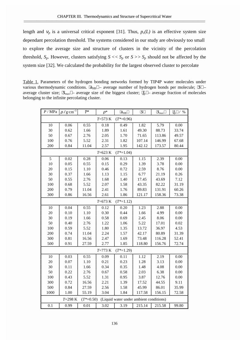
CCHHAAPPTTEERR IIIIII.. TThheerrmmooddyynnaammiiccss aanndd SSttrruuccttuurree ooff SSuuppeerrccrriittiiccaall WWaatteerr————————————————————————————————————————————————————————————————————————————————————————————————————————————————
136
length and νp is a universal critical exponent [31]. Thus, pc(L) is an effective system size
dependant percolation threshold. The systems considered in our study are obviously too small
to explore the average size and structure of clusters in the vicinity of the percolation
threshold, Sp. However, clusters satisfying S << Sp or S >> Sp should not be affected by the
system size [32]. We calculated the probability for the largest observed cluster to percolate
Table 1. Parameters of the hydrogen bonding networks formed by TIP4P water molecules undervarious thermodynamic conditions. ⟨nHB⟩ – average number of hydrogen bonds per molecule; ⟨S⟩ –average cluster size; ⟨Smax⟩ – average size of the biggest cluster; ⟨fp⟩ – average fraction of moleculesbelonging to the infinite percolating cluster.
P / MPa ρ / g·cm–33 ρ* ⟨nHB⟩ ⟨ S⟩ ⟨ Smax⟩ ⟨ fp⟩ / %
T=573 K (T*=0.96)
10 0.06 0.55 0.18 0.49 1.82 5.79 0.0030 0.62 1.66 1.89 1.61 49.30 88.73 33.7450 0.67 2.76 2.05 1.70 71.65 113.86 49.57
100 0.76 5.52 2.31 1.82 107.14 146.99 67.68200 0.84 11.04 2.57 1.95 142.12 173.57 80.44
T=623 K (T*=1.04)
5 0.02 0.28 0.06 0.13 1.15 2.39 0.0010 0.05 0.55 0.15 0.29 1.39 3.78 0.0020 0.15 1.10 0.46 0.72 2.59 8.76 0.0030 0.37 1.66 1.13 1.15 6.77 21.19 0.2650 0.55 2.76 1.68 1.40 17.45 43.69 7.12
100 0.68 5.52 2.07 1.58 43.35 82.22 31.19200 0.79 11.04 2.41 1.76 89.83 131.91 60.26300 0.86 16.56 2.61 1.86 121.17 158.36 73.38
T=673 K (T*=1.12)
10 0.04 0.55 0.12 0.20 1.23 2.88 0.0020 0.10 1.10 0.30 0.44 1.66 4.99 0.0030 0.19 1.66 0.58 0.69 2.45 8.06 0.0050 0.40 2.76 1.22 1.06 5.22 17.01 0.02
100 0.59 5.52 1.80 1.35 13.72 36.97 4.53200 0.74 11.04 2.24 1.57 42.17 80.89 31.39300 0.81 16.56 2.47 1.69 73.48 116.28 52.41500 0.91 27.59 2.77 1.85 118.80 156.76 72.74
T=773 K (T*=1.29)
10 0.03 0.55 0.09 0.11 1.12 2.19 0.0020 0.07 1.10 0.21 0.23 1.28 3.13 0.0030 0.11 1.66 0.34 0.35 1.48 4.08 0.0050 0.22 2.76 0.67 0.58 2.03 6.38 0.00
100 0.43 5.52 1.31 0.95 3.87 12.76 0.00300 0.72 16.56 2.21 1.39 17.52 44.55 9.11500 0.84 27.59 2.56 1.58 45.99 86.01 35.99
1000 1.00 55.19 3.04 1.84 117.58 156.15 72.58
T=298 K (T*=0.50) (Liquid water under ambient conditions)
0.1 0.99 0.01 3.02 3.19 215.14 215.58 99.80
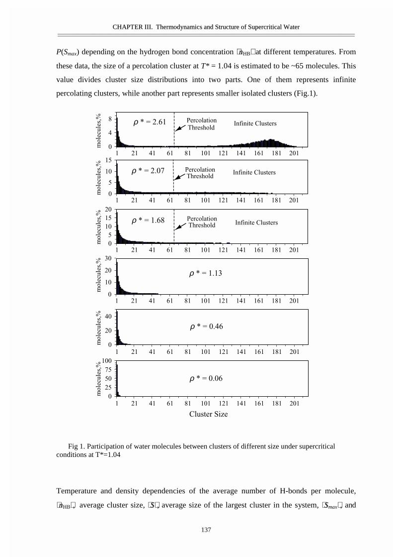
CCHHAAPPTTEERR IIIIII.. TThheerrmmooddyynnaammiiccss aanndd SSttrruuccttuurree ooff SSuuppeerrccrriittiiccaall WWaatteerr————————————————————————————————————————————————————————————————————————————————————————————————————————————————
137
P(Smax) depending on the hydrogen bond concentration ⟨nHB⟩ at different temperatures. From
these data, the size of a percolation cluster at T* = 1.04 is estimated to be ~65 molecules. This
value divides cluster size distributions into two parts. One of them represents infinite
percolating clusters, while another part represents smaller isolated clusters (Fig.1).
Fig 1. Participation of water molecules between clusters of different size under supercriticalconditions at T*=1.04
Temperature and density dependencies of the average number of H-bonds per molecule,
⟨nHB⟩, average cluster size, ⟨S⟩ , average size of the largest cluster in the system, ⟨Smax⟩, and
ρ * = 1.68
0
5
10
15
20
1 21 41 61 81 101 121 141 161 181 201
mole
cule
s,%
PercolationThreshold Infinite Clusters
ρ * = 0.46
0
20
40
1 21 41 61 81 101 121 141 161 181 201
mole
cule
s,%
ρ * = 1.13
0
10
20
30
1 21 41 61 81 101 121 141 161 181 201
mole
cule
s,%
ρ * = 0.06
0
25
50
75
100
1 21 41 61 81 101 121 141 161 181 201
Cluster Size
mole
cule
s,%
ρ * = 2.61
0
4
8
1 21 41 61 81 101 121 141 161 181 201
mole
cule
s,%
Percolation
ThresholdInfinite Clusters
ρ * = 2.07
0
5
10
15
1 21 41 61 81 101 121 141 161 181 201
mole
cule
s,%
PercolationThreshold
Infinite Clusters
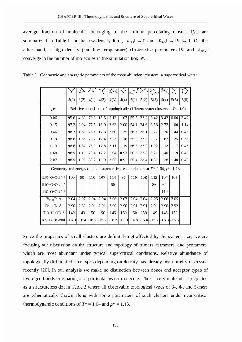
CCHHAAPPTTEERR IIIIII.. TThheerrmmooddyynnaammiiccss aanndd SSttrruuccttuurree ooff SSuuppeerrccrriittiiccaall WWaatteerr————————————————————————————————————————————————————————————————————————————————————————————————————————————————
138
average fraction of molecules belonging to the infinite percolating cluster, ⟨ fp⟩ , are
summarized in Table 1. In the low-density limit, ⟨nHB⟩ → 0 and ⟨Smax⟩ → ⟨S⟩ → 1. On the
other hand, at high density (and low temperature) cluster size parameters ⟨S⟩ and ⟨Smax⟩
converge to the number of molecules in the simulation box, N.
Table 2. Geometric and energetic parameters of the most abundant clusters in supercritical water.
12 2
11
32
3(1) 3(2) 4(1) 4(2) 4(3) 4(4) 5(1) 5(2) 5(3) 5(4) 5(5) 5(6)
ρ* Relative abundance of topologically different water clusters at T*=1.04
0.06 95.6 4.39 78.3 15.5 5.13 1.07 55.5 32.2 3.42 3.42 0.00 3.42
0.15 97.2 2.94 77.5 16.9 3.63 2.00 54.1 34.6 3.58 2.72 1.00 1.14
0.46 98.3 1.69 78.8 17.3 2.60 1.35 56.3 36.1 2.27 1.70 1.44 0.48
0.79 98.6 1.55 79.2 17.4 2.23 1.16 55.9 37.3 2.17 1.67 1.25 0.38
1.13 98.6 1.37 78.9 17.8 2.11 1.19 56.7 37.2 1.92 1.12 1.17 0.46
1.68 98.9 1.15 79.4 17.7 1.94 0.93 56.3 37.3 2.21 1.40 1.19 0.40
2.07 98.9 1.09 80.2 16.9 2.05 0.91 55.4 38.4 1.51 1.38 1.40 0.49
Geometry and energy of small supercritical water clusters at T*=1.04, ρ*=1.13
⟨∠ O··O··O⟩1 / ° 109 60 110 107 114 87 110 108 112 107 105
⟨∠ O··O··O⟩2 / ° 60 86 60
⟨∠ O··O··O⟩3 / ° 119
⟨RO··H⟩ / Å 2.04 2.07 2.04 2.04 2.06 2.03 2.04 2.04 2.05 2.06 2.05
⟨RO··O⟩ / Å 2.90 2.89 2.91 2.91 2.90 2.90 2.91 2.91 2.91 2.90 2.92
⟨∠ O··H–O⟩ / ° 149 143 150 150 146 150 150 150 149 146 150
⟨UHB⟩ / kJ/mol -16.9 -16.4 -16.9 -16.7 -16.3 -17.0 -16.9 -16.8 -16.7 -16.3 -16.8
Since the properties of small clusters are definitely not affected by the system size, we are
focusing our discussion on the structure and topology of trimers, tetramers, and pentamers,
which are most abundant under typical supercritical conditions. Relative abundance of
topologically different cluster types depending on density has already been briefly discussed
recently [20]. In our analysis we make no distinction between donor and acceptor types of
hydrogen bonds originating at a particular water molecule. Thus, every molecule is depicted
as a structureless dot in Table 2 where all observable topological types of 3-, 4-, and 5-mers
are schematically shown along with some parameters of such clusters under near-critical
thermodynamic conditions of T* = 1.04 and ρ* = 1.13.
CCHHAAPPTTEERR IIIIII.. TThheerrmmooddyynnaammiiccss aanndd SSttrruuccttuurree ooff SSuuppeerrccrriittiiccaall WWaatteerr————————————————————————————————————————————————————————————————————————————————————————————————————————————————
139
Only two topologically different types of clusters can be formed by three water molecules: 3-
member rings 3(2) constitute less then 2% of all trimers, while 98% of them are represented
by simple chain-like clusters 3(1). Four water molecules also mainly form chains 4(1) (~80%
of all tetramers) or pyramid-like clusters 4(2) (~17%). More complex clusters containing 3- or
4-member rings, 4(3) and 4(4), constitute together less then 3% of all tetramers. Similarly, the
pentamer distribution mostly consists of linear chains 5(1) (~56%) and branched chains 5(2)
(about 38%). All five other pentamer cluster types (4 of them are shown in Table 2) contribute
together less then 10%. Interestingly, the most branched non-cyclic 5-member cluster, the
tetrahedron-like structure 5(5), represents only ~1% of all pentamers. A noticeable increase of
the fraction of 5-member rings 5(6) is observed with isothermally decreasing density. Thus, 5-
member rings may play an appreciable role in very dilute supercritical water vapor. However,
it is important to keep in mind that at ρ*=0.06, T*=1.04 all possible pentamers contribute just
0.07% to the cluster size distribution, while at ρ*=0.03, T*=1.29 their fraction is only
0.004%. In the latter case, hexamers and larger clusters were not observed at all.
To summarize, H-bonded molecular clusters containing open chain-like or tree-like structures
are found to predominate over clusters containing cyclic ring-like elements. It is observed that
the relative distribution of water molecules between topologically different clusters of same
size is not significantly affected by changes of the thermodynamic conditions – temperature,
pressure, or density. These observations may appear to disagree with the results of ab initio
calculations, which predict ring-like configurations to be the most stable structures [7,8,10].
One might argue that an empirical potential simply fails to describe molecular interaction
adequately enough. However, recent molecular mechanics studies utilizing the TIP4P water
model [33] have successfully predicted global energetic minima for the geometry of water
clusters similar to the results of ab initio simulations [7,8,10,33,34]. Thus, the interaction
potential is not to be blamed. Moreover, our previous analysis of the structure of supercritical
water clusters based on completely different water potential gave almost identical results [20].
The real reason for these discrepancies seems to be in the different settings of two types of
calculations. Ab initio calculations, as well as molecular mechanics modeling, predict static
molecular configurations (minimum energy structures) which are stable in vacuum at 0 K. On
the other hand, molecular clusters obtained by Monte-Carlo and molecular dynamics [20]
simulations are equilibrium “dynamic“ structures, which represent a compromise between
intermolecular (intercluster) interactions, effects of cluster interactions with surrounding
molecules, and thermal kinetic motion. Thus, it is not surprising to observe higher abundance
CCHHAAPPTTEERR IIIIII.. TThheerrmmooddyynnaammiiccss aanndd SSttrruuccttuurree ooff SSuuppeerrccrriittiiccaall WWaatteerr————————————————————————————————————————————————————————————————————————————————————————————————————————————————
140
of 5-member molecular rings at low density in our study. They are predicted to be stable in
vacuum. This observation seems to support our point. There is another possible confusion to
be commented on. Various 4,5,6-member ring-like structures are reported to exist in low
temperature water [35]. However, in the case of liquid water such structures represent only
specific details of an infinite percolating molecular cluster. These structural elements are not
the subject of our study, although it seems safe to believe that they exist in dense supercritical
water, as well. Here we discuss only the structure and topology of isolated water complexes.
We have analyzed several geometric and energetic parameters of hydrogen bonds forming the
most abundant molecular trimers, tetramers and pentamers in supercritical water. The results
for some less abundant pentamers are not reported because of their very rare occurrence and
poor statistics. Average hydrogen-bonding angles ⟨∠ O··O··O⟩ and ⟨∠ O··H–O⟩ , distances
⟨RO··O⟩ and ⟨RO··H⟩, and energies ⟨UHB⟩ are reported in Table 2 for the supercritical
thermodynamic point T*=1.04 and ρ*=1.13. It is noteworthy, that the most abundant clusters,
with topologies 3(1), 4(1), 4(2), 5(1) and 5(2) have almost identical geometric and energetic
characteristics. So, H-bond lengths were found for all clusters to be 2.04 Å, while H-bonding
angles ⟨∠ O··O··O⟩ have values ~109°, which corresponds to the geometry of an ideal
tetrahedrally ordered lattice. Cluster geometry was also studied at other thermodynamic
conditions. With increasing temperature and/or decreasing density H-bond distances ⟨RO··O⟩
and ⟨RO··H⟩ increase, in agreement with other observations [13,14,19]. However, it is quite
remarkable, that average angles ⟨∠ O··O··O⟩ for the most abundant clusters remain almost
constant at ~109° over the whole range of supercritical conditions studied. This result is in
excellent agreement with available X-ray diffraction data for supercritical water [2,36] which
show a noticeable peak of molecular distribution function at ~4.5 Å corresponding to
tetrahedrally ordered second nearest neighbors.
There are two ways to compare energy of clusters – energy per hydrogen bond or energy per
water molecule. Obviously, these quantities are different since clusters of the same size may
have different number of internal bonds. Because cluster definition is based on strength of its
bonds, ⟨UHB⟩ is employed. Generally, one may expect that cluster abundance is proportional
to exp(–βU), where β = (k*T)–1, k – Boltzmann constant, T – temperature and U – potential
energy of intermolecular interactions. At a constant temperature, the most abundant clusters
generally should have lower energy. This assumption, however, is not always supported by
the data in Table 2. So, ⟨UHB3(1)⟩ < ⟨UHB
3(2)⟩, ⟨UHB4(1)⟩ < ⟨UHB
4(2)⟩ < ⟨UHB4(3)⟩ . On the other
CCHHAAPPTTEERR IIIIII.. TThheerrmmooddyynnaammiiccss aanndd SSttrruuccttuurree ooff SSuuppeerrccrriittiiccaall WWaatteerr————————————————————————————————————————————————————————————————————————————————————————————————————————————————
141
hand, ⟨UHB4(4)⟩ < ⟨UHB
4(1)⟩ , in contrast with the low abundance of 4-member rings. Similarly,
⟨UHB5(5)⟩ ≈ ⟨UHB
5(2)⟩ , while the latter topology is much more abundant. Apparently, not only
energetic, but also entropic effects play significant role in determining the abundance of
particular cluster types. For instance, despite the low potential energy of the configuration
5(5), such pentamers can evidently form only when very specific conditions for mutual
distances and angles are satisfied for all 5 molecules forming such a structure.
This work was partly supported by INTAS (grants UA-95-0096 and 96-1989).
REFERENCES
[1] M.M. Hoffmann and M.S. Conradi, J. Am. Chem. Soc., 119, 3811 (1997).
[2] Yu.E. Gorbaty and A.G. Kalinichev, J. Phys. Chem., 99, 5336 (1995).
[3] A.K. Soper, F. Bruni and M.A. Ricci, J. Chem. Phys., 106, 247 (1997).
[4] N. Matubayasi, C. Wakai and M. Nakahara, J. Chem. Phys., 107, 9133 (1997).
[5] J.B. Paul, C.P. Collier, R.J. Saykally, J.J. Sherer, A. O´Keefe, J. Phys. Chem. A, 101, 5211
(1997).
[6] A. Chialvo and P.T. Cummings, J. Chem. Phys., 101, 4466 (1994).
[7] K. Liu, M.G. Brown, J.D. Cruzan, R.J. Saykally, Science, 271, 62 (1996).
[8] K. Liu, J.D. Cruzan, R. J. Saykally, Science, 271, 929 (1996).
[9] J.K. Gregory, D.C. Clary, K. Liu, M.G. Brown, R. J. Saykally, Science, 275, 814 (1997).
[10] K. Liu, M.G. Brown, C. Carter, R.J. Saykally, J.K. Gregory, D.C. Clary, Nature, 381,
501 (1996).
[11] E.S. Fois, M. Sprik and M. Parrinello, Chem. Phys. Lett., 223, 411 (1994).
[12] A. Luzar and D. Chandler Nature, 379, 55 (1996).
[13] A.G. Kalinichev and J.D. Bass, Chem. Phys. Lett., 231, 301 (1994).
[14] T.I. Mizan, P.E. Savage and R.M. Ziff, J. Phys. Chem., 98, 13067 (1994).
[15] G. Löffler, H. Schreiber and O. Steinhauser, Ber. Bunsenges. Phys. Chem., 98, 1575
(1994).
[16] A.G. Kalinichev and K. Heinzinger, Geochim. Cosmochim. Acta., 59, 641 (1995).
[17] R.D. Mountain, J. Chem. Phys., 103, 3084 (1995).
[18] R.D. Mountain, J. Chem. Phys., 110, 2109 (1999).
[19] A.G. Kalinichev and J.D. Bass, J. Phys. Chem. A, 101, 9720 (1997).
CCHHAAPPTTEERR IIIIII.. TThheerrmmooddyynnaammiiccss aanndd SSttrruuccttuurree ooff SSuuppeerrccrriittiiccaall WWaatteerr————————————————————————————————————————————————————————————————————————————————————————————————————————————————
142
[20] A.G. Kalinichev and S.V. Churakov, Chem. Phys. Lett., 302, 411 (1999).
[21] T. Driesner, Science, 277, 791 (1997).
[22] M.P. Allen and D.J. Tildesley, Computer Simulation of Liquids, Oxford University
Press, New York, 1987.
[23] W.L. Jorgensen, J. Chandrasekhar, J.D. Madura, R.W. Impey and M.L. Klein, J Chem.
Phys., 79, 926 (1983).
[24] D. Eisenberg and W. Kautzmann, The Structure and Properties of Water, Oxford
University Press, Oxford, 1969.
[25] A.G. Kalinichev, Z.Naturforschung, 46a, 433 (1991).
[26] Y. Guissani and B. Guillot, J Chem. Phys., 99, 8221 (1993).
[27] J.P. Hansen Phys. Rev. A, 2, 221 (1970).
[28] Pruss, A. and W. Wagner, J. Phys. Chem. Ref. Data (in press);
(available at http://webbook.nist.gov).
[29] M. Sahimi, Applications of Percolation Theory, Taylor & Francis Ltd, 1994.
[30] H.E. Stanley and J. Teixeira, J. Chem. Phys., 73, 3404 (1980).
[31] M. Levinstein, M.S. Shur and E.L. Efros, Soviet Phys.-JETP, 42, 1120 (1976).
[32] D. Stauffer, and A. Aharony, Introduction to percolation theory, Taylor & Francis,
London, 1992.
[33] S.S. Xantheas and T.H. Dunning, Jr. J. Chem. Phys., 99, 8774 (1993).
[34] S.S. Xantheas, J. Chem. Phys., 100, 7523 (1994).
[35] R.J. Speedy, J.D. Madura and W.L. Jorgensen, J. Phys. Chem., 91, 909 (1987).
[36] Yu.E. Gorbaty and Yu.N. Demianets, Chem. Phys. Lett., 100, 450 (1983).
143
LIST OF PUBLICATIONS
1. Shmulovich K.I. & Churakov S.V. (1998) Natural fluid phases at high temperatures and
low pressures. Journal of Geochemical Exploration, 62, 183-191.
2. Kalinichev A.G. & Churakov S.V. (1999) Size and topology of molecular clusters in
supercritical water: A molecular dynamics simulation. Chem. Phys. Letters (302) 5-6, 411-
417.
3. Churakov S.V. & Kalinichev A.G. (1999) Size and structure of molecular clusters in
supercritical water. Journal of Structural Chemistry, 40(4), 548-553.
4. Churakov S.V., Tkachenko S.I., Korzhinskii M.A., Bocharnikov R.E. & Shmulovich K.I.
(2000) Evolution of Composition of High-Temperature Fumarolic Gases from Kudryavy
Volcano, Iturup, Kuril Islands: the Thermodynamic Modeling. Geochemistry International,
38(5), 436-451.
5. Churakov S.V. & Kalinichev A.G. (2000) Size structure and abundance of molecular
clusters in supercritical water over a wide range of densities: Monte-Carlo simulations. In:
Tremaine, P.R, Hill, P.G., Irish, D.E., and Balakrishman, P.V. (Editors). 2000. Steam, Water,
and Hydrothermal systems: Physics and Chemistry Meeting the Needs of Industry. NRC
Research Press, Ottawa, Canada. 418-425.
6. Kalinichev A.G. & Churakov S.V. (2001) Thermodynamics and structure of molecular
clusters in supercritical water. Fluid Phase Equilibria 183–184, 271–278.
7. Frolova T.I., Plechov P.Yu., Tikhomirov P.L., and Churakov S.V. (2001) Melt Inclusions
in Minerals of Allivalites of the Kuril-Kamchatka Island Arc. Geochemistry International,
39(4), 336-346.
8. Churakov S.V. & Gottschalk M. (2001) Perturbation theory based equation of state for
polar molecular fluids. I Pure fluids. Geochimica et Cosmochimica Acta (in press).
9. Churakov S.V. & Gottschalk M. (2001) Perturbation theory based equation of state for
polar molecular fluids. II Fluid mixtures. Geochimica et Cosmochimica Acta (in press).
144
ACKNOWLEDGMENTS
First, I would like to express my deep gratitude to Prof. Dr. Kiril Shumulovich who
has had and still has an enormous influence on the development of my scientific interests
since I first met him as a student. I would also like to acknowledge Dr Sergey I. Tkachenko,
Dr Mikhail A. Korzinskii and all other staff members of the “laboratory of hydrothermal
fluids” of Institute of Experimental Mineralogy (Chernogolovka, Russia) for a very fruitful
collaboration with my computer modeling of the thermodynamic equilibria in volcanic gases.
I am grateful to Prof. Dr. Andrey G. Kalinichev for introducing me to and instructing me in
the field of computer simulations of fluids, as well as constructive criticism of my work and
useful discussions.
Prof. Dr. Wilhelm Heinrich gave me the opportunity to work on my PhD thesis at the
GeoForschungsZentrum, Potsdam and showed an insistent interest in my work. I am highly
indebted to my supervisor PD Dr. Matthias Gottschalk for bringing my thoughts in order and
loosing his nerve cells when correcting my terrible English.
I am also very thankful to all staff members in PB 4.1 of the GeoForschungsZentrum,
namely Ulf Andersson, Ingeborg Bauer, Anne Feenstra, Daniel Harlov, Beate Hein, Stefan
Melzer, Ralf Milke, Hans-Josef Reichmann, Frank Schilling, Christian Schmidt, Reiner
Schulz, Anne-Magali Seydoux, Richard Wirth, and Bernd Wunder for everyday help and
comradeship. Special thanks to PhD students Jens Najorka, Michael Höfer and Birgit Pöter
for explaining to me the tangled and impenetrable rules for living in Germany.

145
CURRICULUM VITAE
Surname: ChurakovGiven Name: SergeyDate of birth: 28 December, 1974Place of birth: Moscow, RussiaCitizenship: Russia FederationOfficial address: GeoForschungsZentrum, Potsdam
Telegrafenberg,D-14473 Potsdam, Germany
E-mail: [email protected]: +49 0331 288 1853Fax: +49 0331 288 1402
Private address: Neuendorfer Str. 10, D-14480 Potsdam, Germany
Scientific carrier:
1991:High School certificate
1991-1997:Student in the Moscow State University
1994-1995:Laboratory in the Institute of Experimental Mineralogy Russia Academy of Science(Chernogolovka Moscow distract, Russia).
1995-1996:Software administrator in Computer Center of Russian Academy of Science.
1996:Graduated from “geological department” of Moscow State University. Diploma inGeochemistry (Equivalent to the Master Degree of Science).
1997:Graduated from “mathematics and computer science department” of Moscow StateUniversity. Diploma in Mathematics (Equivalent to the Master Degree of Science).
1998-2001:PhD student in GeoForschungsZentrum, Potsdam, Germany.

Erklärung
Hiermit erkläre ich an Eides statt, dass ich die vorliegende Arbeit selbständig und nur
mit den angegebenen Mitteln angefertigt habe.
Sergey Churakov