Phylogeography by Diffusion on a Sphere

Remco R. Bouckaertr.bouckaert@auckland.ac.nz

Computational Evolution Group, University of AucklandComputer Science Department, University of Waikato

Institute for History and the Sciences, Max Planck Institute

March 10, 2015

Abstract

Techniques for reconstructing geographical history along a phylogenycan answer many interesting question about the geographical origins ofspecies. Bayesian models based on the assumption that taxa move througha diffusion process have found many applications. However, these methodsrely on diffusion processes on a plane, and do not take the spherical natureof our planet in account. This makes it hard to perform analysis thatcover the whole world, or do not take in account the distortions causedby projections like the Mercator projection.

In this paper, we introduce a Bayesian phylogeographical methodbased on diffusion on a sphere. When the area where taxa are sampledfrom is small, a sphere can be approximated by a plane and the modelresults in the same inferences as with models using diffusion on a plane.For taxa samples from the whole world, we obtain substantial differences.We present an efficient algorithm for performing inference in an MarkovChain Monte Carlo (MCMC) algorithm, and show applications to smalland large samples areas.

Availability: The method is implemented in the GEO SPHERE pack-age in BEAST 2, which is open source licensed under LGPL.

1 Introduction

A number of Bayesian phylogeographical methods have been developed in therecent years [16, 17, 6, 20] that make it convenient to analyse sequence dataassociated with leaf nodes on a tree and infer the geographical origins of thesetaxa. This allows for answering questions about geographical origins of for ex-ample viral outbreaks like Ebola [12], and HIV [11], the Indo-European languagefamily [6] as well as many other species (see [10] for more).

The assumption underlying these methods is that taxa migrate through arandom walk over a plane. This may be appropriate for smaller areas, but whensamples are taken from a large area of the planet, it may be necessary to map

1

.CC-BY-NC-ND 4.0 International licenseis made available under aThe copyright holder for this preprint (which was not peer-reviewed) is the author/funder. It. https://doi.org/10.1101/016311doi: bioRxiv preprint

Figure 1: Left Mercator projection, right Mollweide projection.

part of the planet onto a plane. Figure 1 shows two such projections: the popularMercator projection, which shows large distortions in areas especially around thepoles and the Mollweide projection which ensures equal areas, but distorts therelative positions. Though some projections preserve some metric properties,unfortunately, there is no projection that maintains distances between all pairsof points.

In this paper, we consider random walks over a sphere, instead of over aplane. This is equivalent to assuming a heterogeneous diffusion process over asphere. The benefit is that we do not need to worry about distortions in theprojection. Also, for smaller areas it behaves equivalent to a model assumingdiffusion over a plane, so it can be applied on any scale. Perhaps the most closelyrelated model is described in [9], which uses a less accurate approximation forspherical diffusion and does not work out an efficient inference scheme.

In the next section, we detail the model, which follows the tradition of treat-ing the geography as just another piece of information on each of the leaves inthe tree. In this model, the geography is independent of any sequence infor-mation for the leaves conditioned on the tree. Section 3 has implementationdetails for using the model efficiently with MCMC. We develop an approximatelikelihood that can be calculated efficiently and relies on setting the internallocations to their (weighted) mean values. We compare results between planarand spherical diffusion in a simple simulation study and analyse the origin ofHepatitis B in Section 4, then wrap up with a discussion and conclusions.

2 The spherical diffusion model

In this section, we explain the details of the spherical diffusion model and howto apply it to phylogeography. We assume homogeneous diffusion over a sphere,governed by a single parameter, the precision D of the diffusion process. Forsuch diffusion, the probability density of making a move over angle α at time t

2

.CC-BY-NC-ND 4.0 International licenseis made available under aThe copyright holder for this preprint (which was not peer-reviewed) is the author/funder. It. https://doi.org/10.1101/016311doi: bioRxiv preprint

1e−06 1e−02 1e+02 1e+06

1e−08

1e−04

1e+00

0.0

0.4

0.8

1.0

0.0 0 .5 1 .0 1 .5 2 .0 2 .5 3 .0

0.0

0.5

1.0

1.5 =0.1

=1τ

τ

Figure 2: Topt, 1/N (τ) (y-axis) for different values of τ = D/t (x-axis) on alog-log scale (left axis, solid line) and normal-log scale (right axis, dashed line).Bottom, density functions (y-axis) for spherical diffusion (solid lines) and planardiffusion (dashed lines) with τ = 0.1 and τ = 1.0. The x-axis is the angle forspherical diffusion and distance to start point for planar diffusion.

is closely approximated by [18]:

p(α|D, t) =Nτ

√sin(α)α e−

α2

2τ (1)

where N is a normalising condition such that∫ π0dαf(α|D, t) = 1 and τ =

Dt . Figure 2 shows the shape of N for different values of τ calculated using

numeric integration in R. For small values of τ (< 10−6) we found that N isapproximately 1 (> 0.9999999), while for large values of τ (> 106)N approaches2.88266

τ within a relative error bounded by 10−6. In between we can pre-calculate

the values of τ in the range 2a/2 for a ∈ {−40, 60} and get reasonably closevalues by interpolating between these samples, since the function of N in τ isvery smooth.

Figure 2 shows the difference between a density function with precision 1 andat time 1 for both planar diffusion and spherical diffusion. Spherical diffusion

3

.CC-BY-NC-ND 4.0 International licenseis made available under aThe copyright holder for this preprint (which was not peer-reviewed) is the author/funder. It. https://doi.org/10.1101/016311doi: bioRxiv preprint

peaks a bit earlier, but planar diffusion has a longer tail. This intuitively makessense; there is less space on a sphere when moving out 1 unit than on a plane,so a slightly earlier peak is expected. Also, for a long distances on a sphere onarrives on the other side at a smaller angel, once the sphere is traversed to theother side.

Let T be a binary tree over a set of n taxa x1, . . . , xn. Internal nodes of thetree are numbered n+ 1, . . . , 2n− 1. With each node xi is associated a location(lati, longi) with latitude lati and longitude longi.

p(T |D) =∏

i=1...2n−1

f(xi|θ,D) (2)

where D the precision of the diffusion process and θ other parameters, likebranch length, etc., and f(xi|θ,D) defined as

f(xi|θ,D) =

{proot(xi) if xi is rootp(αi|D, ti) otherwise

(3)

with proot(.) the root density, and p(αi|D, ti) the spherical density of Equation1 and αi the angle between location of xi and its parent, and ti the ’length’of the branch. This length is equal to the clock rate used for the branch timesthe length of the branch in the tree. For instance for a strict clock with rate r,the length is simply equal to the branch length in time times r. More relaxedmodels like the uncorrelated relaxed clock [8], have individual rates that candiffer for each branch.

For the root density proot(.), we usually take the uniform prior, indicat-ing we have no preference where the root locations is placed. This simplifiesEquation (2) in that the first term becomes a constant, which can be ignoredduring MCMC sampling. Using more complex priors can have consequence forinference, as outlined in Section 3.3.

To determine the angle between two locations (lat1, long1) and (lat2, long2)requires a bit of based geometry:

α = arccos(sin(lat1) sin(lat2) + cos(long1) cos(long2) cos(lat2 − lat1)

).

A common situation is where we have a tree where the leaf nodes have knownpoint loctions and we want to infer the locations of internal nodes, in particularthe root location which represents the origin of all taxa associated with leafnodes in the tree. The tree is typically informed by sequence information Dassociated with the leaf nodes.

3 Implementation

The simplest, and in many ways most flexible, approach is to explicitly maintainall locations as part of the state. Calculation of the likelihood for geography

4

.CC-BY-NC-ND 4.0 International licenseis made available under aThe copyright holder for this preprint (which was not peer-reviewed) is the author/funder. It. https://doi.org/10.1101/016311doi: bioRxiv preprint

on a tree using Equation 2 (up to a constant) becomes straightforward. Unfor-tunately, designing MCMC proposals that efficiently sample the state space ishard.

3.1 Particle filter approach

The particle filter method [7] is another way of calculating the likelihood withoutexplicit representation of the locations. For every sample in the MCMC chain,the likelihood is calculated based on the tree as informed by other data. Asa result, the MCMC has a lot lower change of getting stuck in local maximaand less care is required in designing efficient proposals for dealing with thegeography.

To calculate the likelihood, we use a number of ’particles’ and each particlerepresents the locations of each of the nodes in the tree. Locations of internalnodes are initialised by setting them to the mean locations of their childrenin a post-order traversal of the tree, which results in a sufficiently good fitof locations to the tree to guarantee quick convergence. Next, particles areperturbed in pre-order traversal as follows: for a location of node xi, randomlyk locations are sampled in the vicinity of the current location. Out of the klocations, one location is sampled proportional to the partial fit of the location.This partial fit is simply the contribution the location provides to the density(Equation (2)) consisting of

p(αi|D, ti)p(αleft(i)|D, tleft(i))p(αright(i)|D, tright(i))

where xleft(i) is the left child of xi and xright(i) its right child. For the rootnode p(αi|D, ti) is assumed to be constant.

After all particles are perturbed, an equally sized set of particles is sampled(with replacement) from the current set, with probability proportional to thedensity as defined by Equation (2). This process quickly converges to a stablelikelihood. Furthermore, it does not easily get stuck in local maxima. Unfortu-nately, in the context of the MCMC algorithm where the likelihood needs to berecalculated many times, this process is still rather slow.

Therefore, we explore an approximation based on assigning mean locationsto each of the internal nodes.

3.2 Mean location approximation

Suppose we want to calculate the mean location for each internal node definedas

lati = lilatL(i) + rilatR(i) + pilatP (i) (4)

longi = lilongL(i) + rilongR(i) + pilongP (i) (5)

and at the root node as

lati = lilatL(i) + rilatR(i) (6)

longi = lilongL(i) + rilongR(i) (7)

5

.CC-BY-NC-ND 4.0 International licenseis made available under aThe copyright holder for this preprint (which was not peer-reviewed) is the author/funder. It. https://doi.org/10.1101/016311doi: bioRxiv preprint

Figure 3: Left, the mean of two blue points by taking the mean lati-tude/longitude is the red point, while the green point is closer. Right, takingthe mean location of 2 and 3 points on a sphere.

where L(i), R(i) and P (i) the index of left and right child and parent of xirespectively and li, ri and pi are positive weights associated with first andsecond child and parent respectively that add to unity (li + ri + pi = 1).

So, we have a set of n − 1 linear equations in n − 1 unknown values forlatitude, and the same for longitude. We can solve these with standard methodsfor solving linear equations such as Gaussian elimination in O(n3), but thestructure of the tree allows us to solve this problem more in linear time (O(n))as follows.

First, do a post order traversal where for each node, we send a message (mi,ρi) to the parent where if xi is a leaf node,

mi = lati

ρi = 0

and if xi is not a leaf node,

mi =limL(i) + rimR(i)

1− liρL(i) − riρR(i)

ρi =1

1− liρL(i) − riρR(i)

At the root, we have

lati =limL(i) + rimR(i)

1− liρL(i) − riρR(i)(8)

Next, we do a pre-order traversal from the root, sending down the latitude,and calculate for all internal nodes (but not leaf nodes)

lati = mi + ρilatP (i) (9)

Theorem 1. Using the above calculations lati is as defined in Equations (4)and (6) and is calculated in O(n).

6

.CC-BY-NC-ND 4.0 International licenseis made available under aThe copyright holder for this preprint (which was not peer-reviewed) is the author/funder. It. https://doi.org/10.1101/016311doi: bioRxiv preprint

5 10 15 20 25

510

15

20

25

−130 −120 −110 −100 −90 −80

−130

−110

−90

−80

Figure 4: Particle filter (horizontal) vs mean approximation (vertical) on a logof log-likelihood scale. Left, sampled from prior, right sampled from posterior(in blue). Also right particle filter vs particle filter (in red) to show stochasticityof particle filter.

See Appendix A for a proof.Especially close to the poles, taking the average point between to pairs of

latitude/longitude pairs can be a point that is far from the point with theshortest distance to these points. For example the points (45, 0) and (45, 180)(blue points in Figure 3) on opposite sides of the pole have a mean of (45, 90)(red point)– a point at the same latitude – while the pole (90, 0) (green point)has a shorter distance to these two points.

Instead of using latitude/longitude to represent location, we can use Carte-sian coordinates (x, y, z) on a sphere. We can convert (lat, long) locationsto Cartesian using (x, y, z) = (sin(θ) cos(φ), sin(θ) sin(φ), cos(θ)) where θ =longπ/180 and φ = (90− lat)π/180. To convert a Cartesian point back to lati-tude/longitude, we use (lat, long) = (arccos(−z)180/π−90, arctan 2(y, x)180/π).

However, the mean of two points on a sphere is not necessarily on a sphere.However, if we take the mean of two points and project it onto a sphere bytaking the intersection of the sphere with a line through the origin and themean point, we get the point that has shortest distance to both points.

Figure 4 shows the likelihood calculated through the particle filter approxi-mation and the mean location approximation outlined above. When samplingfrom the prior, the correlation is almost perfect, while when sampling from theposterior, the mean approximation shows a slight bias. However, also shown inFigure 4 is how well the particle filter correlates with itself. Due to the stochas-tic nature of the algorithm, this correlation is not 100%, and only slightly betterthan the correlation with the mean approximation approach.

In summary, we can use the mean approximation to determine locationsof internal nodes using a fast O(n) algorithm and use Equation 2 with theselocations to approximate the likelihood. The only geography specific parameter

7

.CC-BY-NC-ND 4.0 International licenseis made available under aThe copyright holder for this preprint (which was not peer-reviewed) is the author/funder. It. https://doi.org/10.1101/016311doi: bioRxiv preprint

to be sampled by the MCMC is the precision parameter for the diffusion process.To log locations so that we can reconstruct the geography, logging the meanapproximations would result in biased estimates of the uncertainty in locations.To prevent this, the particle filter is run for those samples that are logged andone of the particles containing all internal locations is used as representativesample for a particular state of the MCMC. Since the particle filter only needsto be run when a state is logged, this is sufficiently computationally efficient tobe practical.

3.3 Refinements

The mean approximation outlined in the previous subsection assumes tips havefixed positions and all internal nodes have not. If tips are not point locations,but sampled from a region with known boundaries, for example a country orprovince, the tips can be sampled using a uniform prior over the region it isknown to be sampled from. A random walk proposal for tips can be used tosample tip locations. The mean approximation runs as before, but obviouslywhen a tip is updated, the tip location needs to be fixed at the new location forthe algorithm.

Suppose a uniform prior for the root is not appropriate, but a region isknown to which the root can be confined. The mean-approximation will assigna value to the root location without concern for such prior and it may assign alocation to the root outside the known region. However, if the root location isrepresented explicitly as part of the state for the MCMC algorithm, the meanapproximation can use that location in its likelihood calculation instead the onerepresented by Equations (6) and (7). Like tip locations, the root location canbe sampled. A distribution representing whether the root locations is in theregion can be added to the prior.

The same technique can be applied if the region of a clade represented by aset of taxa is known. Such location can be explicitly modeled in the state andthe mean approximation, instead of using Equations (4) and (5).

4 Results

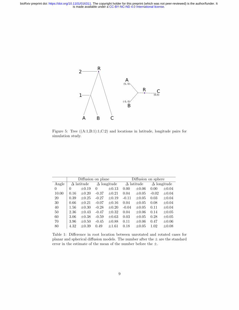
To compare the planar and spherical diffusion models, we run an MCMC anal-ysis with both models using a fixed tree with three taxa that are positioned ona sphere around the location (0, 0) (see Figure 5). The same coordinates werethen placed on the sphere, the sphere rotated towards the south pole in stepsof 10 degrees up to 80 degrees and resulting latitude and longitude positionsused for A, B and C. One would expect when inferring the root locations (R inFigure 5) that rotating it back with the same angle would result in inferring thesame root location as for the unrotated problem. So, the great circle distancebetween the taxa A, B and C does not change when rotated.

Table 1 shows the difference in original root and unrotated root. The planardiffusion shows a significant difference in the estimate of the latitude, while

8

.CC-BY-NC-ND 4.0 International licenseis made available under aThe copyright holder for this preprint (which was not peer-reviewed) is the author/funder. It. https://doi.org/10.1101/016311doi: bioRxiv preprint

A B C

1

2

A

B

C

(5,-5)

(-5,-5)

(0,5)

R

R

Figure 5: Tree ((A:1,B:1):1,C:2) and locations in latitude, longitude pairs forsimulation study.

Diffusion on plane Diffusion on sphereAngle ∆ latitude ∆ longitude ∆ latitude ∆ longitude0 0 ±0.19 0 ±0.13 0.00 ±0.06 0.00 ±0.0410.00 0.16 ±0.20 -0.37 ±0.21 0.04 ±0.05 -0.02 ±0.0420 0.39 ±0.25 -0.27 ±0.19 -0.11 ±0.05 0.03 ±0.0430 0.66 ±0.21 -0.07 ±0.16 0.04 ±0.05 0.08 ±0.0440 1.56 ±0.30 -0.28 ±0.20 -0.04 ±0.05 0.11 ±0.0450 2.36 ±0.43 -0.47 ±0.32 0.04 ±0.06 0.14 ±0.0560 3.06 ±0.38 -0.59 ±0.63 0.03 ±0.05 0.28 ±0.0570 3.96 ±0.50 -0.45 ±0.88 0.11 ±0.06 0.47 ±0.0680 4.32 ±0.39 0.49 ±1.61 0.18 ±0.05 1.02 ±0.08

Table 1: Difference in root location between unrotated and rotated cases forplanar and spherical diffusion models. The number after the ± are the standarderror in the estimate of the mean of the number before the ±.

9

.CC-BY-NC-ND 4.0 International licenseis made available under aThe copyright holder for this preprint (which was not peer-reviewed) is the author/funder. It. https://doi.org/10.1101/016311doi: bioRxiv preprint

Den

sity

posterior-70 -60 -50 -40 -30 -20 -10 0 1 0 2 00

0.25

0.5

0.75

1

1.25

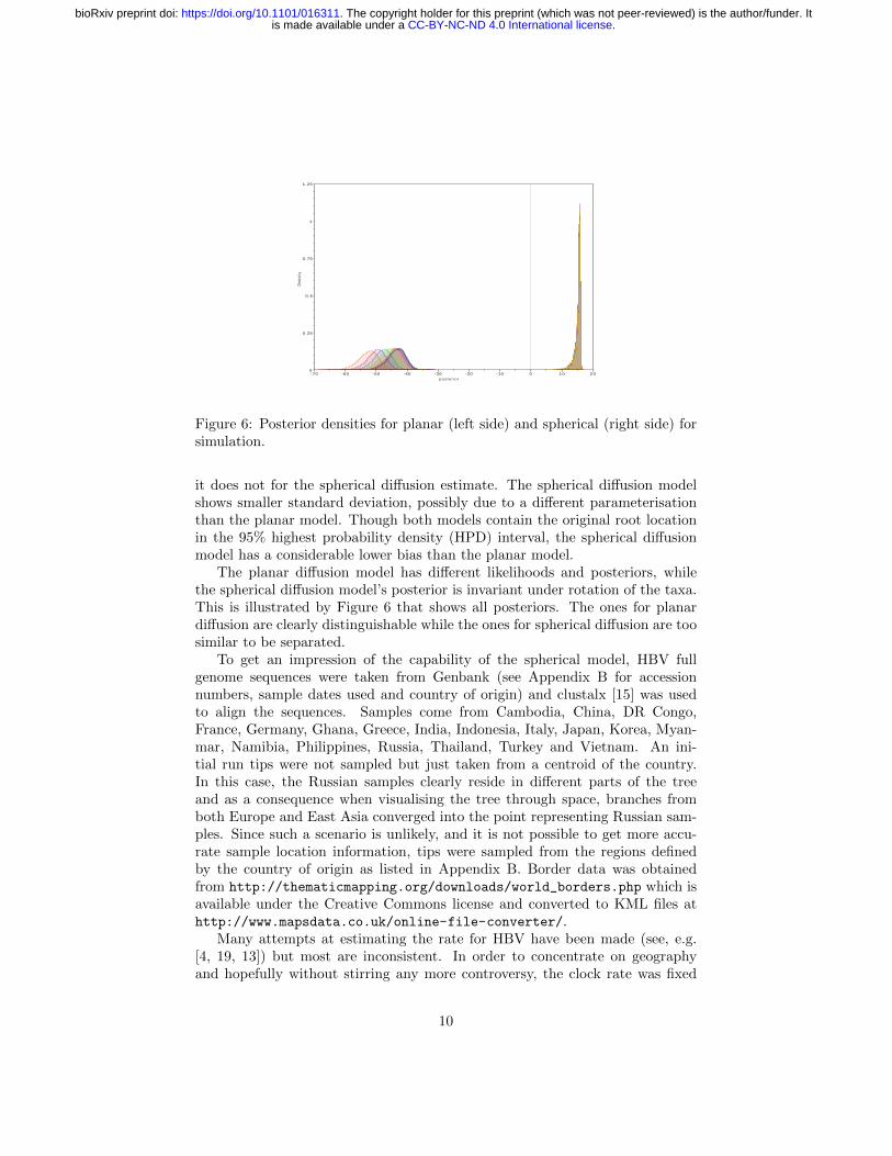
Figure 6: Posterior densities for planar (left side) and spherical (right side) forsimulation.

it does not for the spherical diffusion estimate. The spherical diffusion modelshows smaller standard deviation, possibly due to a different parameterisationthan the planar model. Though both models contain the original root locationin the 95% highest probability density (HPD) interval, the spherical diffusionmodel has a considerable lower bias than the planar model.

The planar diffusion model has different likelihoods and posteriors, whilethe spherical diffusion model’s posterior is invariant under rotation of the taxa.This is illustrated by Figure 6 that shows all posteriors. The ones for planardiffusion are clearly distinguishable while the ones for spherical diffusion are toosimilar to be separated.

To get an impression of the capability of the spherical model, HBV fullgenome sequences were taken from Genbank (see Appendix B for accessionnumbers, sample dates used and country of origin) and clustalx [15] was usedto align the sequences. Samples come from Cambodia, China, DR Congo,France, Germany, Ghana, Greece, India, Indonesia, Italy, Japan, Korea, Myan-mar, Namibia, Philippines, Russia, Thailand, Turkey and Vietnam. An ini-tial run tips were not sampled but just taken from a centroid of the country.In this case, the Russian samples clearly reside in different parts of the treeand as a consequence when visualising the tree through space, branches fromboth Europe and East Asia converged into the point representing Russian sam-ples. Since such a scenario is unlikely, and it is not possible to get more accu-rate sample location information, tips were sampled from the regions definedby the country of origin as listed in Appendix B. Border data was obtainedfrom http://thematicmapping.org/downloads/world_borders.php which isavailable under the Creative Commons license and converted to KML files athttp://www.mapsdata.co.uk/online-file-converter/.

Many attempts at estimating the rate for HBV have been made (see, e.g.[4, 19, 13]) but most are inconsistent. In order to concentrate on geographyand hopefully without stirring any more controversy, the clock rate was fixed

10

.CC-BY-NC-ND 4.0 International licenseis made available under aThe copyright holder for this preprint (which was not peer-reviewed) is the author/funder. It. https://doi.org/10.1101/016311doi: bioRxiv preprint

AB026814HPBC6T588

AB198079

AB198077

AB198080AB205123

AB198083

AF182802D28880

HPBB4HST1HPBC4HST2

AB198084AB198081AB198082AB198078AB111125

AB033550AB049609

AB033556AY641560

AB111121AY641558AB205124AY641559AY641563AY641561

AY641562

HPBB5HKO1HPBC5HKO2

AB198076AB049610AB115417

AB111946AB112063

AB112472AJ748098

AB112065AB205125

AB112066

AB112348AB112408

AB112471AB117758

DQ315781DQ315783DQ315782

AB033554AB033555

AB219426AB219429AB219427AB219428

AB115551

AB205122AB212626

AB212625AB117759

AB205119AB205120

AF121243

AF121245AF121246

AF121244

AF121247AF121251AF121248

AF121249AF121250

AB126580AB205118

AY738143

DQ315784DQ315785HPBADWZCGDQ315786

AB106564

AB205129AB205192AB205188AB205189AB205191AB205190

AY738147DQ060825

DQ060824

DQ060826

DQ060828DQ060829

DQ060827

AB109475AB119254

AB109476AB205126

AB116266

AB109477

AB110075

AB119251AB119253

AB119252AB120308

AB109479

AB109478AB119255AB119256AB188241

AB188242AB205128

AB205127

AY341335AY796031

AB126581

AY721609AY721607

AY721605

AY721606AY721608

AY721611

AY721612AY796030DQ315778

AB188243AB188245DQ315777AJ344117DQ315776

DQ315779DQ315780

AB179747AB205010

Figure 7: DensiTree of Hepatitis B in Eurasia and Africa.

at 2.0E-5 substitutions/site/year, but results can be scaled to what the readerdeems more appropriate.

We used BEAST 2 [5] to perform the analysis with the GTR substitutionmodel with gamma rate heterogeneity with 4 categories and invariant sites.The uncorrelated relaxed clock with log normal distribution [8] was used andshows a coefficient of variation with of mean 0.476 and 95% HPD Interval of(0.3721, 0.5715), which means a strict clock can be ruled out. A coalescent withconstant population size was used as tree prior. The spherical model was runwith a strict clock and a relaxed log normal clock. The AICM values [1] of thestrict clock was 69215 ± 0.93 while that of the relaxed clock was 69086 ± 2.063thus favouring the relaxed clock with a difference of over 128.

Figure 7 shows the DensiTree [3] of the HBV analysis, which demonstratesit is fairly well resolved, with many clades having 100% posterior support.

Figure 8 shows the tree mapped onto the earth after processing with SPREAD[2] and visualised with google-earth. The root of the tree and thus the associ-ated origin of the virus is placed in northern India about 10000 year ago. Figure8 shows the spread at times -4000 CE, -1000 CE, 1000 CE and present. Also

11

.CC-BY-NC-ND 4.0 International licenseis made available under aThe copyright holder for this preprint (which was not peer-reviewed) is the author/funder. It. https://doi.org/10.1101/016311doi: bioRxiv preprint

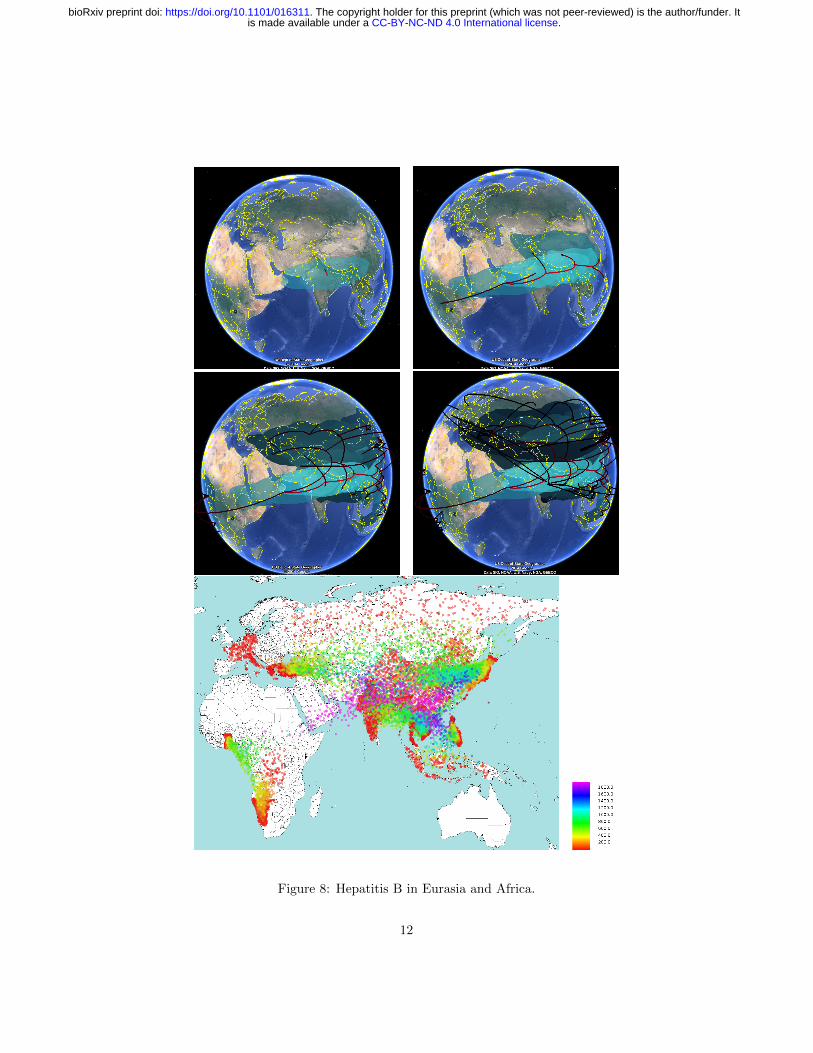
Figure 8: Hepatitis B in Eurasia and Africa.

12

.CC-BY-NC-ND 4.0 International licenseis made available under aThe copyright holder for this preprint (which was not peer-reviewed) is the author/funder. It. https://doi.org/10.1101/016311doi: bioRxiv preprint

shown is a heat map visualising the internal node positions of the trees in tree setrepresenting the posterior. Colours indicate age of the internal node as shownin the legend. It suggests that most of the spread happened relatively recentlyin the last 2000 years. Most of Africa remains white due to lack of samples inthe data set in those areas.

5 Discussion

The spherical diffusion model can be used for phylogeographical analyses insituations similar to where the models of [16, 17] are used that are assumingdiffusion on a plane. Furthermore, the spherical diffusion model can be usedwhen the area of interest is large, and there is considerable distortion when thearea is projected on a plane.

However, it assumes heterogeneous diffusion over a sphere. This meansthat, unlike the models from [16, 17], no distinction is made between possiblecorrelations in the direction of the random walk. Furthermore, the random walkon a sphere assumes a Gaussian distribution with relatively thin tails comparedto a Levy jump process on a plane [20]. Also, it assumes heterogeneous diffusion,unlike the landscape aware model [6].

The spherical diffusion model assumes locations in continuous space, whichtends to be more powerful than using discrete locations. However, it also meansthat phylogeographical approaches based on the structured coalescent [14] can-not be applied, hence demographic developments are not captured by the geo-graphical process.

The method is implemented in the GEO SPHERE package in BEAST 2[5, 10], which is open source licensed under LGPL. An analysis can be set upusing BEAUti, the graphical user interface for BEAST. A tutorial explaininghow to use the method and set up an analysis is available from http://beast2.

org/wiki/tutorials.Results can be visualised using Google-earth after processing with SPREAD

[2].

6 Conclusions

We presented a new way to perform Bayesian phylogeographical analyses basedon diffusion on a sphere. An approximation of the likelihood that can be cal-culated efficiently was presented, which can be used in an MCMC frameworkand is implemented in BEAST 2. The framework allows branch rate modelsin order to relax the strict clock assumption, as well as efficient sampling whenprior information in the form of sampling regions for tip, root or monophyleticclade locations is available.

Further investigations include incorporating inheterogeneous random walksto represent more realistic diffusion processes that distinguish different ratesamong land and water, among forests and deserts, etc.

13

.CC-BY-NC-ND 4.0 International licenseis made available under aThe copyright holder for this preprint (which was not peer-reviewed) is the author/funder. It. https://doi.org/10.1101/016311doi: bioRxiv preprint

Acknowledgements

Joseph Heled helped a lot with many lively discussions on this topic. This re-search was funded by Marsden grant (UOA1308) (http://www.royalsociety.org.nz/programmes/funds/marsden/awards/2013-awards/), a Rutherford fel-lowship (http://www.royalsociety.org.nz/programmes/funds/rutherford-discovery/)from the Royal Society of New Zealand awarded to Prof. Alexei Drummond. Itwas also funded by the Max Planck Institute.

References

[1] G. Baele, P. Lemey, T. Bedford, A. Rambaut, M. A. Suchard, and A. V.Alekseyenko. Improving the accuracy of demographic and molecular clockmodel comparison while accommodating phylogenetic uncertainty. Mol.Biol. Evol., 29(9):2157–2167, 2012.

[2] Filip Bielejec, Andrew Rambaut, Marc A Suchard, and Philippe Lemey.Spread: spatial phylogenetic reconstruction of evolutionary dynamics.Bioinformatics, 27(20):2910–2912, 2011.

[3] Remco Bouckaert and Joseph Heled. Densitree 2: Seeing trees through theforest. doi:10.1101/012401, bioRxiv, 2014.

[4] Remco R. Bouckaert, Monica Alvarado-Mora, and Joao Rebello Pinho.Evolutionary rates and hbv: issues of rate estimation with bayesian molec-ular methods. Antiviral therapy, 2013.

[5] Remco R. Bouckaert, Joseph Heled, Denise Kuhnert, Tim Vaughan, Chieh-Hsi Wu, Dong Xie, Marc A Suchard, Andrew Rambaut, and Alexei J Drum-mond. Beast 2: a software platform for bayesian evolutionary analysis.PLoS Comput Biol, 10(4):e1003537, Apr 2014.

[6] Remco R. Bouckaert, Philippe Lemey, Michael Dunn, Simon J. Greenhill,Alexander V. Alekseyenko, Alexei J. Drummond, Russell D. Gray, Marc A.Suchard, and Quentin D. Atkinson. Mapping the origins and expansion ofthe indo-european language family. Science, 337(6097):957–960, 2012.

[7] Arnaud Doucet, Nando De Freitas, and Neil Gordon. Sequential MonteCarlo methods in practice. Springer, 2001.

[8] Alexei J Drummond, Simon Y W Ho, Matthew J Phillips, and AndrewRambaut. Relaxed phylogenetics and dating with confidence. PLoS Biol,4(5):e88, May 2006.

[9] Alexei James Drummond et al. Computational Statistical Inference forMolecular Evolution and Population Genetics. PhD thesis, ResearchSpace@Auckland, 2002.

14

.CC-BY-NC-ND 4.0 International licenseis made available under aThe copyright holder for this preprint (which was not peer-reviewed) is the author/funder. It. https://doi.org/10.1101/016311doi: bioRxiv preprint

[10] Alexei K. Drummond and Remco R. Bouckaert. Computational evolutionwith BEAST 2. Cambrige University Press, 2014.

[11] Nuno R Faria, Andrew Rambaut, Marc A Suchard, Guy Baele, TrevorBedford, Melissa J Ward, Andrew J Tatem, Joao D Sousa, Nimalan Ari-naminpathy, Jacques Pepin, et al. The early spread and epidemic ignitionof hiv-1 in human populations. science, 346(6205):56–61, 2014.

[12] Stephen K Gire, Augustine Goba, Kristian G Andersen, Rachel SG Seal-fon, Daniel J Park, Lansana Kanneh, Simbirie Jalloh, Mambu Momoh,Mohamed Fullah, Gytis Dudas, et al. Genomic surveillance elucidatesebola virus origin and transmission during the 2014 outbreak. Science,345(6202):1369–1372, 2014.

[13] Abby Harrison, Philippe Lemey, Matthew Hurles, Chris Moyes, SusanneHorn, Jan Pryor, Joji Malani, Mathias Supuri, Andrew Masta, BurentauTeriboriki, et al. Genomic analysis of hepatitis b virus reveals antigen stateand genotype as sources of evolutionary rate variation. Viruses, 3(2):83–101, 2011.

[14] R. R. Hudson. Gene genealogies and the coalescent process. In D Futuymaand J Antonovics, editors, Oxford surveys in evolutionary biology, volume 7,pages 1 – 44. Oxford University Press, Oxford, 1990.

[15] M.A. Larkin, G. Blackshields, N.P. Brown, R. Chenna, P.A. McGettigan,H. McWilliam, F. Valentin, I.M. Wallace, A. Wilm, R. Lopez, J.D. Thomp-son, T.J. Gibson, and D.G. Higgins. Clustal w and clustal x version 2.0.Bioinformatics, 23:2947–2948, 2007.

[16] Philippe Lemey, Andrew Rambaut, Alexei J Drummond, and Marc ASuchard. Bayesian phylogeography finds its roots. PLoS Comput Biol,5(9):e1000520, Sep 2009.

[17] Philippe Lemey, Andrew Rambaut, John J Welch, and Marc A Suchard.Phylogeography takes a relaxed random walk in continuous space and time.Mol Biol Evol, Mar 2010.

[18] Seoul Mapo-gu. A gaussian for diffusion on the sphere. arXiv:1303.1278v1,6 Mar 2013.

[19] Dimitrios Paraskevis, Gkikas Magiorkinis, Emmanouil Magiorkinis, Si-mon YW Ho, Robert Belshaw, Jean-Pierre Allain, and Angelos Hatzakis.Dating the origin and dispersal of hepatitis b virus infection in humans andprimates. Hepatology, 57(3):908–916, 2013.

[20] Oliver G Pybus, Marc A Suchard, Philippe Lemey, Flavien J Bernardin,Andrew Rambaut, Forrest W Crawford, Rebecca R Gray, Nimalan Ari-naminpathy, Susan L Stramer, Michael P Busch, et al. Unifying the spatialepidemiology and molecular evolution of emerging epidemics. Proceedingsof the National Academy of Sciences, 109(37):15066–15071, 2012.

15

.CC-BY-NC-ND 4.0 International licenseis made available under aThe copyright holder for this preprint (which was not peer-reviewed) is the author/funder. It. https://doi.org/10.1101/016311doi: bioRxiv preprint

Appendix A: Proof of Theorem 1

Proof. First, we show that Equation (9) and (8) are valid for any internal nodexi when calculated by post-order traversal. When we reach xi it can be aninternal node or the root node. If xi is an internal node, we distinguish betweenthe children being leaf nodes or internal nodes. Images for Figure 1 were takenfrom Wikipedia.

1) xL(i) and xR(i) are leaf nodes. Then Equation (4) gives, (using latL(i) =mL(i), latR(i) = mR(i) for child nodes xL(i) and xR(i), and the definition of mi

and ρi)

lati = lilatL(i) + rilatR(i) + pilatP (i)

= limL(i) + rimR(i) + pilatP (i)

=lL(i)mL(i) + rR(i)mR(i)

1− lL(i)0− rR(i)0+

pi1− lL(i)0− rR(i)0

latP (i)

= mi + ρilatP (i)

2) xL(i) is a leaf and xR(i) an internal node. Then, latR(i) = mR(i)+ρR(i)lati(by post-order traversal) and latL(i) = mL(i). Then Equation (4) gives,

lati = lilatL(i) + rilatR(i) + pilatP (i)

= limL(i) + ri(mR(i) + ρR(i)lati) + pilatP (i)

grouping lati and divide by 1− 0− riρR(i) gives

lati =lL(i)mL(i) + rR(i)mR(i)

1− lL(i)0− rR(i)ρR(i)+

pi1− lL(i)0− rR(i)ρR(i)

latP (i)

=lL(i)mL(i) + rR(i)mR(i)

1− lL(i)ρL(i) − rR(i)ρR(i)+

pi1− lL(i)ρL(i) − rR(i)ρR(i)

latP (i)

= mi + ρilatP (i)

3) xL(i) is an internal node and xR(i) a leaf node. By symmetry, case 2holds.

4) xL(i) and xR(i) are both internal nodes. Then, latL(i) = mL(i) + ρL(i)latiand latR(i) = mR(i)+ρR(i)lati(by post-order traversal). Now Equation (4) gives,

lati = lilatL(i) + rilatR(i) + pilatP (i)

= li(mL(i) + ρL(i)lati) + ri(mR(i) + ρR(i)lati) + pilatP (i)

grouping lati and divide by 1− liρL(i) − riρR(i) gives

lati =lL(i)mL(i) + rR(i)mR(i)

1− lL(i)ρL(i) − rR(i)ρR(i)+

pi1− lL(i)ρL(i) − rR(i)ρR(i)

latP (i)

= mi + ρilatP (i)

16

.CC-BY-NC-ND 4.0 International licenseis made available under aThe copyright holder for this preprint (which was not peer-reviewed) is the author/funder. It. https://doi.org/10.1101/016311doi: bioRxiv preprint

If xi is the root Equation (8) follows from a similar argument, but withρi = 0.

From equations Equations (9) and (8) together it follows that the mean canbe calculated by post-order traversal to provide information for the root location(8) to be calculated, followed by a pre-order traversal to calculate locations ofinternal nodes using (9).

Complexity: it is easy to see the algorithm is O(n) since it takes one post-order traversal sending 2n − 2 messages up and one pre-order traversal calcu-lating locations for n− 1 internal nodes. Each message and latitude calculationis O(1).

17

.CC-BY-NC-ND 4.0 International licenseis made available under aThe copyright holder for this preprint (which was not peer-reviewed) is the author/funder. It. https://doi.org/10.1101/016311doi: bioRxiv preprint

Appendix B: HBV data

Genbank year location

AB026814 1998 JapanAB033550 1988 JapanAB033554 1985 IndonesiaAB033555 1984 IndonesiaAB033556 1985 JapanAB049609 1996 JapanAB049610 1996 JapanAB106564 1999 GhanaAB109475 2001 JapanAB109476 1997 JapanAB109477 1997 JapanAB109478 1998 JapanAB109479 1997 JapanAB110075 2001 JapanAB111121 1998 JapanAB111125 2001 JapanAB111946 1998 VietnamAB112063 1998 VietnamAB112065 1998 VietnamAB112066 1999 MyanmarAB112348 1999 MyanmarAB112408 1999 MyanmarAB112471 2002 ThailandAB112472 2002 ThailandAB115417 1996 JapanAB115551 2004 CambodiaAB116266 1987 JapanAB117758 2004 CambodiaAB117759 2004 CambodiaAB119251 2002 JapanAB119252 2002 JapanAB119253 2000 JapanAB119254 2003 JapanAB119255 2001 JapanAB119256 1997 JapanAB120308 1982 JapanAB126580 2000 RussiaAB126581 2000 RussiaAB179747 2002 ItalyAB188241 1999 JapanAB188242 1999 JapanAB188243 1999 JapanAB188245 2000 Japan

Genbank year location

AB198076 2001 ChinaAB198077 2001 ChinaAB198078 2001 ChinaAB198079 2001 ChinaAB198080 2001 ChinaAB198081 2001 ChinaAB198082 2001 ChinaAB198083 2001 ChinaAB198084 2001 ChinaAB205010 1994 JapanAB205118 2001 JapanAB205119 2000 JapanAB205120 2000 JapanAB205122 2001 VietnamAB205123 2002 ChinaAB205124 2003 JapanAB205125 2001 VietnamAB205126 2001 JapanAB205127 2000 RussiaAB205128 2000 RussiaAB205129 1999 GhanaAB205188 2000 GhanaAB205189 2000 GhanaAB205190 2000 GhanaAB205191 2000 GhanaAB205192 2000 GhanaAB212625 2004 VietnamAB212626 2004 VietnamAB219426 2002 PhilippinesAB219427 2002 PhilippinesAB219428 2002 PhilippineAB219429 2002 PhilippinesAF121243 1995 VietnamAF121244 1993 VietnamAF121245 1992 VietnamAF121246 1998 VietnamAF121247 1994 VietnamAF121248 1994 VietnamAF121249 1998 VietnamAF121250 1997 VietnamAF121251 1997 VietnamAF182802 1992 ChinaAJ344117 1990 France

Genbank year location

AJ748098 2002 VietnamAY341335 2003 GreeceAY641558 2003 KoreaAY641559 2003 KoreaAY641560 2003 KoreaAY641561 2003 KoreaAY641562 2003 KoreaAY641563 2003 KoreaAY721605 2004 TurkeyAY721606 2004 TurkeyAY721607 2004 TurkeyAY721608 2004 TurkeyAY721609 2004 TurkeyAY721611 2004 TurkeyAY721612 2004 TurkeyAY738143 1997 GermanyAY738147 1998 DR CongoAY796030 2004 TurkeyAY796031 2004 TurkeyD23680 1991 JapanD23681 1992 JapanD23682 1984 JapanD23683 1984 JapanD23684 1988 JapanD28880 1992 JapanDQ060824 1983 NamibiaDQ060825 1983 NamibiaDQ060826 1983 NamibiaDQ060827 1983 NamibiaDQ060828 1983 NamibiaDQ060829 1983 NamibiaDQ315776 2000 IndiaDQ315777 2003 IndiaDQ315778 2003 IndiaDQ315779 2003 IndiaDQ315780 2002 IndiaDQ315781 2003 IndiaDQ315782 2004 IndiaDQ315783 2003 IndiaDQ315784 2003 IndiaDQ315785 2003 IndiaDQ315786 2005 IndiaM57663 1987 Philippines

18

.CC-BY-NC-ND 4.0 International licenseis made available under aThe copyright holder for this preprint (which was not peer-reviewed) is the author/funder. It. https://doi.org/10.1101/016311doi: bioRxiv preprint