Phylogenetic AnalysisPhylogenetic AnalysisUnit 16Unit 16

BIOL221TBIOL221T: Advanced : Advanced Bioinformatics for Bioinformatics for

BiotechnologyBiotechnologyIrene Gabashvili, PhD

B&O, chapter 14B&O, chapter 14

Bioinformatics analyses should be Bioinformatics analyses should be interpreted in evolutionary contextinterpreted in evolutionary context

Good-quality sequence alignments Good-quality sequence alignments important for evolutionary analysisimportant for evolutionary analysis

Common phylogenetic methods and Common phylogenetic methods and software are different – be cautious software are different – be cautious when using and interpreting your when using and interpreting your resultsresults

Terminology and the Terminology and the BasicsBasics

Phylogenetics is sometimes called Phylogenetics is sometimes called claudisticsclaudistics

Clade – a set of descendants from a Clade – a set of descendants from a single ancestor (greek for branch).single ancestor (greek for branch).

3 basic assumptions:3 basic assumptions: Any group of organism descended from a Any group of organism descended from a

common ancestorcommon ancestor Bifurcating pattern of cladogenesisBifurcating pattern of cladogenesis Change in characteristics occurs in lineages Change in characteristics occurs in lineages

over timeover time

Brief Brief Introduction to Introduction to

the Theory of the Theory of EvolutionEvolution

Classification: LinnaeusClassification: Linnaeus

Carl LinnaeusCarl Linnaeus1707-17781707-1778

Classification: LinnaeusClassification: Linnaeus• Hierarchical systemHierarchical system

– KingdomKingdom (Rige)(Rige)– PhylumPhylum (Række)(Række)– ClassClass (Klasse)(Klasse)– OrderOrder (Orden)(Orden)– FamilyFamily (Familie)(Familie)– GenusGenus (Slægt)(Slægt)– SpeciesSpecies (Art)(Art)

Classification depicted Classification depicted as a treeas a tree

Classification depicted Classification depicted as a treeas a tree

SpeciesSpecies GenusGenus FamilyFamily OrderOrder ClassClass

Theory of evolutionTheory of evolution

Charles DarwinCharles Darwin1809-18821809-1882

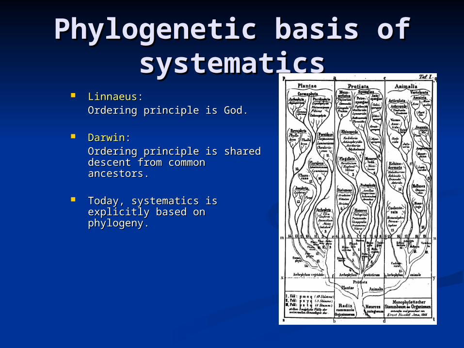
Phylogenetic basis of Phylogenetic basis of systematicssystematics

LinnaeusLinnaeus: : Ordering principle is God.Ordering principle is God.

DarwinDarwin: : Ordering principle is shared Ordering principle is shared descent from common ancestors.descent from common ancestors.

Today, systematics is explicitly Today, systematics is explicitly based on phylogeny.based on phylogeny.

Darwin’s four postulatesDarwin’s four postulates

I.I. More young are produced each generation than More young are produced each generation than can survive to reproduce.can survive to reproduce.

II.II. Individuals in a population vary in their Individuals in a population vary in their characteristics.characteristics.

III.III. Some differences among individuals are based Some differences among individuals are based on genetic differences.on genetic differences.

IV.IV. Individuals with favorable characteristics have Individuals with favorable characteristics have higher rates of survival and reproduction.higher rates of survival and reproduction.

Evolution by means of natural selectionEvolution by means of natural selection Presence of ”design-like” features in organisms:Presence of ”design-like” features in organisms:

quite often features are there “for a reason”quite often features are there “for a reason”

Theory of evolution as Theory of evolution as the basis of biological the basis of biological

understandingunderstanding

”Nothing in biology makes sense, except in the light of evolution.

Without that light it becomes a pile of sundry facts - some of them interesting or curious but making no meaningful picture as a whole”

T. Dobzhansky

Phylogenetic Phylogenetic Reconstruction:Reconstruction:Distance Matrix Distance Matrix

MethodsMethods

Trees: terminologyTrees: terminology

TerminologyTerminology

Clades – monophyletic taxonClades – monophyletic taxon Taxons – any named group of Taxons – any named group of

organismorganism Branches – divergence (length may Branches – divergence (length may

indicate the degree)indicate the degree) Nodes – any bifurcating branch pointNodes – any bifurcating branch point

Trees: terminologyTrees: terminology

Trees: representationsTrees: representations

Three different representations of the same tree

Trees: rooted vs. Trees: rooted vs. unrootedunrooted

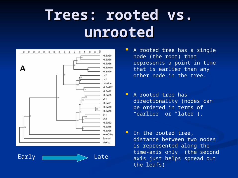
A rooted tree has a single node (the root) that represents a point in time that is earlier than any other node in the tree.

A rooted tree has directionality (nodes can be ordered in terms of “earlier” or “later”).

In the rooted tree, distance between two nodes is represented along the time-axis only (the second axis just helps spread out the leafs)

Early Late

Trees: rooted vs. Trees: rooted vs. unrootedunrooted

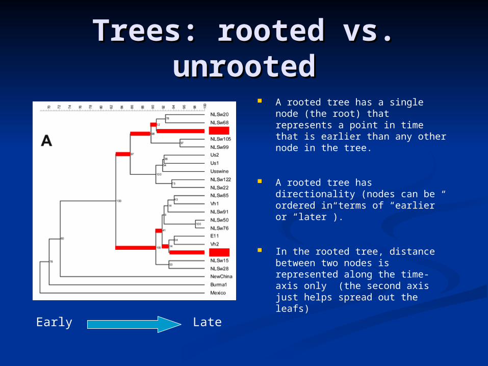
A rooted tree has a single node (the root) that represents a point in time that is earlier than any other node in the tree.

A rooted tree has directionality (nodes can be ordered in terms of “earlier” or “later”).

In the rooted tree, distance between two nodes is represented along the time-axis only (the second axis just helps spread out the leafs)

Early Late

Trees: rooted vs. Trees: rooted vs. unrootedunrooted

A rooted tree has a single node (the root) that represents a point in time that is earlier than any other node in the tree.

A rooted tree has directionality (nodes can be ordered in terms of “earlier” or “later”).

In the rooted tree, distance between two nodes is represented along the time-axis only (the second axis just helps spread out the leafs)

Early Late

Trees: rooted vs. Trees: rooted vs. unrootedunrooted

In unrooted trees there is no directionality: we do not know In unrooted trees there is no directionality: we do not know if a node is earlier or later than another nodeif a node is earlier or later than another node

Distance along branches directly represents node distanceDistance along branches directly represents node distance

Trees: rooted vs. Trees: rooted vs. unrootedunrooted

In unrooted trees there is no directionality: we do not know In unrooted trees there is no directionality: we do not know if a node is earlier or later than another nodeif a node is earlier or later than another node

Distance along branches directly represents node distanceDistance along branches directly represents node distance

Reconstructing a tree Reconstructing a tree using non-using non-

contemporaneous datacontemporaneous data

Reconstructing a tree using present-day Reconstructing a tree using present-day datadata

Data: molecular Data: molecular phylogenyphylogeny

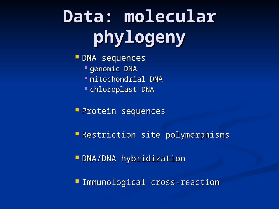
DNA sequencesDNA sequences genomic DNAgenomic DNA mitochondrial DNAmitochondrial DNA chloroplast DNAchloroplast DNA

Protein sequencesProtein sequences

Restriction site polymorphismsRestriction site polymorphisms

DNA/DNA hybridizationDNA/DNA hybridization

Immunological cross-reactionImmunological cross-reaction

Morphology vs. Morphology vs. molecular datamolecular data

African white-backed vulture(old world vulture)

Andean condor (new world vulture)

New and old world vultures seem to be closely related based on morphology.

Molecular data indicates that old world vultures are related to birds of prey (falcons, hawks, etc.) while new world vultures are more closely related to storks

Similar features presumably the result of convergent evolution

Molecular data: single-Molecular data: single-celled organismscelled organisms

Molecular data useful for analyzing single-celled organisms (which have only few prominent morphological features).

Distance Matrix MethodsDistance Matrix Methods

1.1. Construct multiple Construct multiple alignment of sequencesalignment of sequences

2.2. Construct table listing all Construct table listing all pairwise differences pairwise differences (distance matrix)(distance matrix)

3.3. Construct tree from Construct tree from pairwise distancespairwise distances

Gorilla : ACGTCGTAHuman : ACGTTCCTChimpanzee: ACGTTTCG

GoGo HuHu ChCh

GoGo -- 44 44

HuHu -- 22

ChCh --

Go

Hu

Ch

2

11

1

Finding Optimal Branch Finding Optimal Branch LengthsLengths

SS11 SS22 SS33 SS44

SS11 -- DD1212 DD1313 DD1414

SS22 -- DD2323 DD2424

SS33 -- DD3434

SS44 --Observed distance

S1

S3

S2

S4

a

b

c

d e

Distance along tree

D12 d12 = a + b + cD13 d13 = a + dD14 d14 = a + b + eD23 d23 = d + b + cD24 d24 = c + eD34 d34 = d + b + e

Goal:

Optimal Branch Optimal Branch Lengths: Least SquaresLengths: Least Squares

Fit between given tree Fit between given tree and observed distances and observed distances can be expressed as “sum can be expressed as “sum of squared differences”:of squared differences”:

Q = Q = (D(Dijij - d - dijij))22

Find branch lengths that Find branch lengths that minimize Q - this is the minimize Q - this is the optimal set of branch optimal set of branch lengths for this tree.lengths for this tree.

S1

S3

S2

S4

a

b

c

d e

Distance along tree

D12 d12 = a + b + cD13 d13 = a + dD14 d14 = a + b + eD23 d23 = d + b + cD24 d24 = c + eD34 d34 = d + b + e

Goal:

j>i

Least Squares Optimality Least Squares Optimality CriterionCriterion

Search through all (or many) tree topologiesSearch through all (or many) tree topologies

For each investigated tree, find best branch For each investigated tree, find best branch lengths using least squares criterionlengths using least squares criterion

Among all investigated trees, the best tree is Among all investigated trees, the best tree is the one with the smallest sum of squared the one with the smallest sum of squared errors. errors.

Exhaustive search impossible for large Exhaustive search impossible for large data setsdata sets

No. No. taxataxa

No. treesNo. trees

33 11

44 33

55 1515

66 105105

77 945945

88 10,39510,395

99 135,135135,135

1010 2,027,0252,027,025

1111 34,459,42534,459,425

1212 654,729,075654,729,075

1313 13,749,310,57513,749,310,575

1414 316,234,143,225316,234,143,225

1515 7,905,853,580,6257,905,853,580,625

Heuristic searchHeuristic search

1.1. Construct initial tree; determine sum of squaresConstruct initial tree; determine sum of squares

2.2. Construct set of “neighboring trees” by making small Construct set of “neighboring trees” by making small rearrangements of initial tree; determine sum of squares for rearrangements of initial tree; determine sum of squares for each neighboreach neighbor

3.3. If any of the neighboring trees are better than the initial tree, If any of the neighboring trees are better than the initial tree, then select it/them and use as starting point for new round of then select it/them and use as starting point for new round of rearrangements. (Possibly several neighbors are equally good)rearrangements. (Possibly several neighbors are equally good)

4.4. Repeat steps 2+3 until you have found a tree that is better Repeat steps 2+3 until you have found a tree that is better than all of its neighbors.than all of its neighbors.

5.5. This tree is a “local optimum” (not necessarily a global This tree is a “local optimum” (not necessarily a global optimum!) optimum!)

Clustering AlgorithmsClustering Algorithms Starting point: Distance matrixStarting point: Distance matrix

Cluster least different pair of sequences:Cluster least different pair of sequences: Tree: pair connected to common ancestral node, compute branch Tree: pair connected to common ancestral node, compute branch

lengths from ancestral node to both descendantslengths from ancestral node to both descendants

Distance matrix: combine two entries into one. Compute new distance Distance matrix: combine two entries into one. Compute new distance

matrix, by finding distance from new node to all other nodesmatrix, by finding distance from new node to all other nodes

Repeat until all nodes are linkedRepeat until all nodes are linked

Results in only one tree, there is no measure of tree-Results in only one tree, there is no measure of tree-goodness.goodness.

Neighbor Joining Neighbor Joining AlgorithmAlgorithm

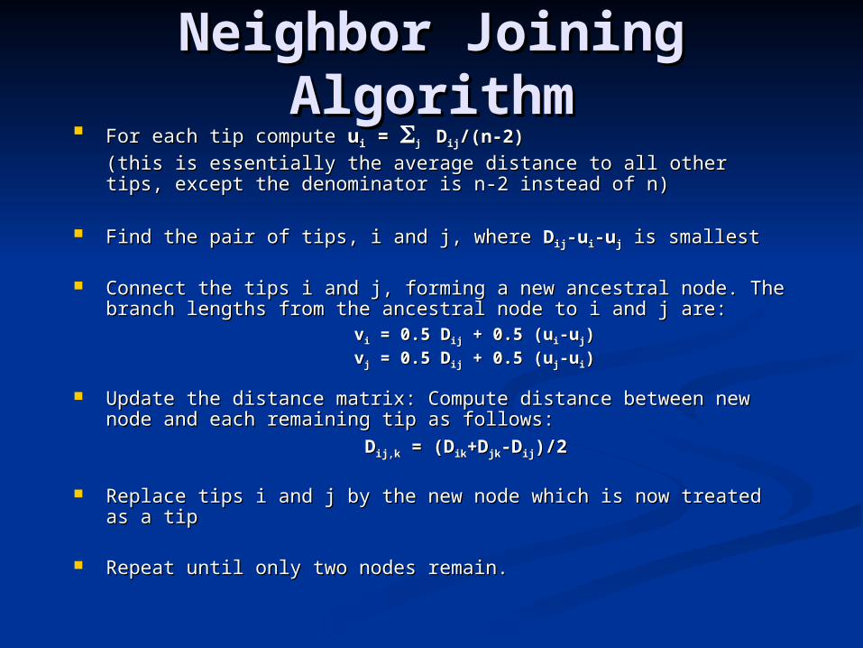
For each tip compute For each tip compute uuii = = jj DDijij/(n-2)/(n-2)

(this is essentially the average distance to all other tips, except the (this is essentially the average distance to all other tips, except the denominator is n-2 instead of n)denominator is n-2 instead of n)

Find the pair of tips, i and j, where Find the pair of tips, i and j, where DDijij-u-uii-u-ujj is smallest is smallest

Connect the tips i and j, forming a new ancestral node. The branch Connect the tips i and j, forming a new ancestral node. The branch lengths from the ancestral node to i and j are:lengths from the ancestral node to i and j are:

vvii = 0.5 D = 0.5 Dijij + 0.5 (u + 0.5 (uii-u-ujj))

vvjj = 0.5 D = 0.5 Dijij + 0.5 (u + 0.5 (ujj-u-uii))

Update the distance matrix: Compute distance between new node and Update the distance matrix: Compute distance between new node and each remaining tip as follows:each remaining tip as follows:

DDij,kij,k = (D = (Dikik+D+Djkjk-D-Dijij)/2)/2

Replace tips i and j by the new node which is now treated as a tipReplace tips i and j by the new node which is now treated as a tip

Repeat until only two nodes remain.Repeat until only two nodes remain.

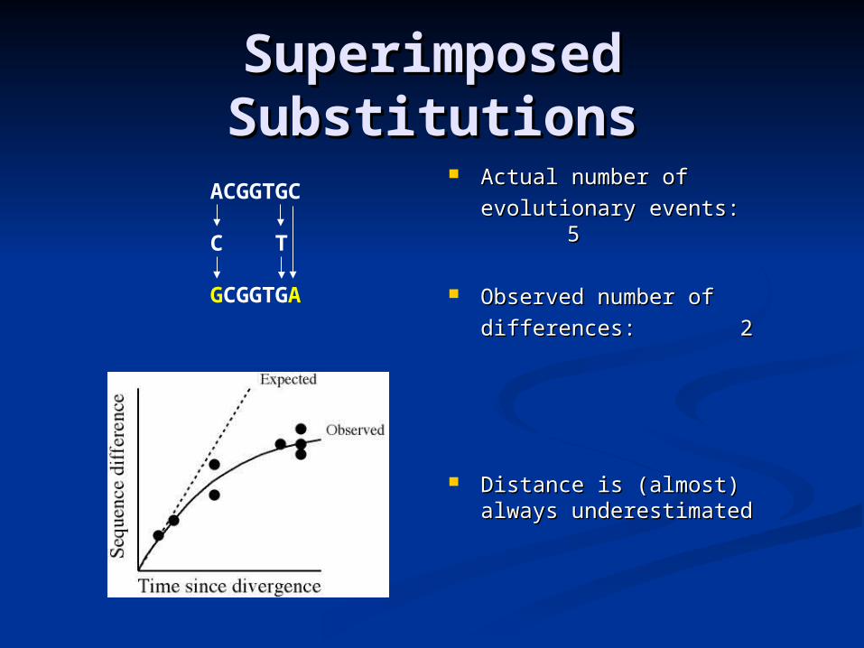
Superimposed Superimposed SubstitutionsSubstitutions

Actual number of Actual number of

evolutionary events:evolutionary events: 55

Observed number of Observed number of

differences:differences: 22

Distance is (almost) always Distance is (almost) always underestimatedunderestimated

ACGGTGC

C T

GCGGTGA

Model-based correction Model-based correction for for

superimposed superimposed substitutionssubstitutions Goal: try to infer the real number of Goal: try to infer the real number of

evolutionary events (the real evolutionary events (the real distance) based ondistance) based on

1.1. Observed data (sequence alignment)Observed data (sequence alignment)

2.2. A model of how evolution occursA model of how evolution occurs

Jukes and Cantor ModelJukes and Cantor Model Four nucleotides assumed to Four nucleotides assumed to

be equally frequent (f=0.25)be equally frequent (f=0.25)

All 12 substitution rates All 12 substitution rates assumed to be equalassumed to be equal

Under this model the Under this model the corrected distance is:corrected distance is:

DDJCJC = -0.75 x ln(1-1.33 x = -0.75 x ln(1-1.33 x DDOBSOBS))

For instance:For instance:

DDOBSOBS=0.43 => D=0.43 => DJCJC=0.64=0.64

A C G T

A -3

C -3

G -3

T -3

Other models of Other models of evolutionevolution

HomologsHomologs

Orthologs - speciationOrthologs - speciation Paralogs - duplicationParalogs - duplication Xenologs – horizontal transferXenologs – horizontal transfer

Clustering AlgorithmsClustering Algorithms

Clustering algorithms use distances to Clustering algorithms use distances to calculate phylogenetic trees. These calculate phylogenetic trees. These trees are based solely on the relative trees are based solely on the relative numbers of similarities and differences numbers of similarities and differences

between a set of sequences.between a set of sequences. Start with a matrix of pairwise distancesStart with a matrix of pairwise distances

Cluster methods construct a tree by linking Cluster methods construct a tree by linking the least distant pairs of taxa, followed by the least distant pairs of taxa, followed by successively more distant taxa. successively more distant taxa.

From Multiple Sequence From Multiple Sequence AlignmentAlignment

Best cluster: {ATCC,ATGC}Best cluster: {ATCC,ATGC}

ATCC ATGC TTCG TCGG

ATCC 0 1 2 4

ATGC 0 3 3

TTCG 0 2

TCGG 0

{ATCC,ATGC} TTCG TCGG

{ATCC,ATGC}

0 ½(2+3)=2.5

½(4+3)=3.5

TTCG 0 2

TCGG 0 Best cluster: {TTCG,TCGG}Best cluster: {TTCG,TCGG}

ExampleExample

{ATCC,ATGC} {TTCG,TCG{TTCG,TCGG}G}

{ATCC,ATGC} 0 ½(2.5+3.5)=3

{TTCG,TCGG} 0

ATCC ATGC TTCG ATCC ATGC TTCG TCGGTCGG

1.5 1.5

0.50.51 1

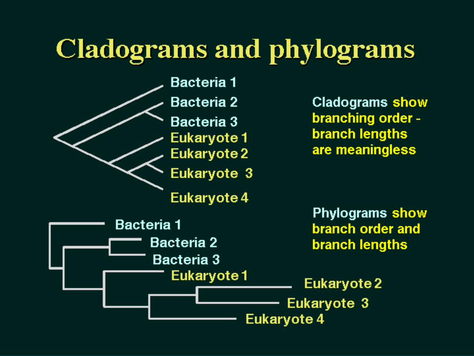
A Cladogram or a Phylogram?

Cladistic MethodsCladistic Methods Evolutionary relationships are documented Evolutionary relationships are documented

by creating a branching structure, termed by creating a branching structure, termed a phylogeny or tree, that illustrates the a phylogeny or tree, that illustrates the relationships between the sequences. relationships between the sequences.

CladisticCladistic methods construct a tree methods construct a tree ((cladogramcladogram) by considering the various ) by considering the various possible pathways of evolution and choose possible pathways of evolution and choose from among these the best possible tree.from among these the best possible tree.

A A phylogramphylogram is a tree with branches that is a tree with branches that are proportional to evolutionary distances.are proportional to evolutionary distances.

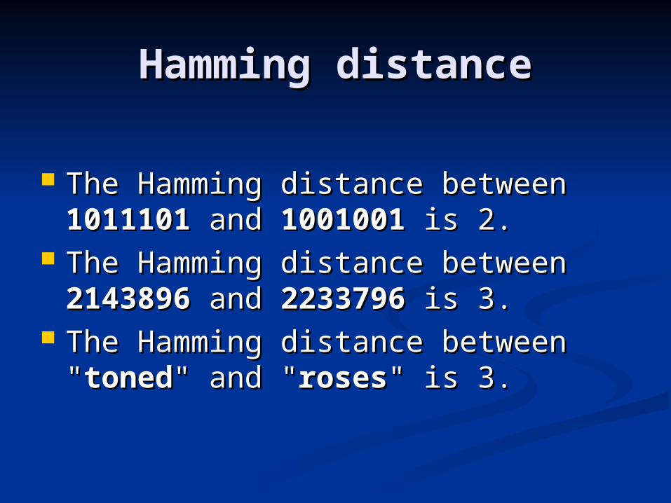
Hamming distanceHamming distance

<between two strings of equal <between two strings of equal length>: the number of positions for length>: the number of positions for which the corresponding symbols which the corresponding symbols are different. The number of are different. The number of substitutionssubstitutions required to change one required to change one into the other, or the number of into the other, or the number of errorserrors that transformed one string that transformed one string into the other.into the other.

Hamming distanceHamming distance

The Hamming distance between The Hamming distance between 10111011011101 and and 10010011001001 is 2. is 2.

The Hamming distance between The Hamming distance between 21438962143896 and and 22337962233796 is 3. is 3.

The Hamming distance between The Hamming distance between ""tonedtoned" and "" and "rosesroses" is 3. " is 3.

Levenshtein DistanceLevenshtein Distance

A measure of the similarity between two A measure of the similarity between two strings: number of deletions, insertions, or strings: number of deletions, insertions, or substitutionssubstitutions

For example, For example, If s is "test" and t is "test", then LD(s,t) = If s is "test" and t is "test", then LD(s,t) =

0, 0, If s is "test" and t is "tent", then LD(s,t) = If s is "test" and t is "tent", then LD(s,t) =

1, because one substitution (change "s" to 1, because one substitution (change "s" to "n") is sufficient to transform s into t. "n") is sufficient to transform s into t.

If s os “test” and t is “attempt”, LD(s,t)=4If s os “test” and t is “attempt”, LD(s,t)=4

Levenshtein distanceLevenshtein distance

The Levenshtein distance algorithm The Levenshtein distance algorithm has been used in: has been used in:

Spell checking Spell checking Speech recognition Speech recognition DNA analysis DNA analysis Plagiarism detection Plagiarism detection

DNA DistancesDNA Distances

Distances between pairs of DNA sequences are Distances between pairs of DNA sequences are usually computed as the sum of all base pair usually computed as the sum of all base pair differences between the two sequences. differences between the two sequences. If sequences are similar enough to be alignedIf sequences are similar enough to be aligned

Generally all base changes are considered Generally all base changes are considered equalequal

Insertion/deletions are generally given a larger Insertion/deletions are generally given a larger weight than replacements (gap penalties).weight than replacements (gap penalties).

It is also possible to correct for multiple It is also possible to correct for multiple substitutions at a single site, which is common substitutions at a single site, which is common in distant relationships and for rapidly evolving in distant relationships and for rapidly evolving sites.sites.

Phylogenetic methods (1)

Distance matrix/cluster (UPGMA, NJ):Bacterial taxonomy based on morphological, chemical, biochemical and physiological chacters did not allow natural relationships to be deduced

Numerical taxonomy (Sneath and Sokal, 1963, 1973)

Parsimony (maximum parsomony)The taxonomy of animals shall reflect their natural relatioonships

Phylogenetic Systematics (Willi Hennig 1950, 1966)Without direction (eg. Wiley 1980)

UPGMAUPGMA

The simplest of the distance methods is the The simplest of the distance methods is the UPGMAUPGMA ( (UUnweighted nweighted PPair air GGroup roup MMethod using ethod using AArithmetic averages)rithmetic averages)

The The PHYLIPPHYLIP programs programs DNADISTDNADIST and and PROTDISTPROTDIST calculate absolute pairwise distances between a calculate absolute pairwise distances between a group of sequences. Then the group of sequences. Then the GCGGCG program program GROWTREEGROWTREE uses uses UPGMAUPGMA to build a tree. to build a tree.

Many multiple alignment programs such as Many multiple alignment programs such as PILEUPPILEUP use a variant of use a variant of UPGMAUPGMA to create a to create a dendrogram of DNA sequences which is then used dendrogram of DNA sequences which is then used to guide the multiple alignment algorithm.to guide the multiple alignment algorithm.

Neighbor JoiningNeighbor Joining

The The Neighbor JoiningNeighbor Joining method is the most method is the most popular way to build trees from distance popular way to build trees from distance measurements measurements

(Saitou and Nei 1987, Mol. Biol. Evol. 4:406)(Saitou and Nei 1987, Mol. Biol. Evol. 4:406) Neighbor JoiningNeighbor Joining corrects the UPGMA method for its corrects the UPGMA method for its

(frequently invalid) assumption that the same rate of (frequently invalid) assumption that the same rate of evolution applies to each branch of a tree.evolution applies to each branch of a tree.

The distance matrix is adjusted for differences in the rate of The distance matrix is adjusted for differences in the rate of evolution of each taxon (branch).evolution of each taxon (branch).

Neighbor JoiningNeighbor Joining has given the best results in simulation has given the best results in simulation studies and it is the most computationally efficient of the studies and it is the most computationally efficient of the distance algorithms distance algorithms (N. Saitou and T. Imanishi, Mol. Biol. Evol. 6:514 (N. Saitou and T. Imanishi, Mol. Biol. Evol. 6:514 (1989)(1989)

Cladistic methods Cladistic methods

CladisticCladistic methods are based on the assumption methods are based on the assumption that a set of sequences evolved from a common that a set of sequences evolved from a common ancestor by a process of mutation and selection ancestor by a process of mutation and selection without mixing (hybridization or other horizontal without mixing (hybridization or other horizontal gene transfers).gene transfers).

These methods work best if a specific tree, or at These methods work best if a specific tree, or at least an ancestral sequence, is already known so least an ancestral sequence, is already known so that comparisons can be made between a finite that comparisons can be made between a finite number of alternate trees rather than calculating number of alternate trees rather than calculating all possible trees for a given set of sequences. all possible trees for a given set of sequences.

ParsimonyParsimony

ParsimonyParsimony is the most popular method is the most popular method for reconstructing ancestral for reconstructing ancestral relationships.relationships.

ParsimonyParsimony allows the use of all known allows the use of all known evolutionary information in building a evolutionary information in building a treetree

In contrast, distance methods compress all of In contrast, distance methods compress all of the differences between pairs of sequences the differences between pairs of sequences into a single numberinto a single number

Building Trees with Building Trees with ParsimonyParsimony ParsimonyParsimony involves evaluating all involves evaluating all

possible trees and giving each a score possible trees and giving each a score based on the number of evolutionary based on the number of evolutionary changes that are needed to explain the changes that are needed to explain the observed data. observed data.

The best tree is the one that requires The best tree is the one that requires the fewest base changes for all the fewest base changes for all sequences to derive from a common sequences to derive from a common ancestor.ancestor.

MethodsMethods

Distance-based: UPGMA, NJ, FM, Distance-based: UPGMA, NJ, FM, MEME

Other: Maximum Parsimony, ML, etcOther: Maximum Parsimony, ML, etc

Neighbor JoiningNeighbor Joining methods generally produce just one tree, methods generally produce just one tree, which can help to validate a tree built with the which can help to validate a tree built with the parsimonyparsimony or or maximum likelihoodmaximum likelihood method method

Phylogenetic methods

Maximum likelihood methodsPhylogenies should be formulated in a probalistic framework and statistically testable. Protein and DNA sequence data are extraordinary goodfor phylogenetic interpreation and can ”resist” such treatment.

Cavalli-Sforza and Edwards 1967 (theory)

Felsenstein 1981 first practically useful algorithms.

Phylogenetic analysis.Phylogenetic analysis. Comparison of phylogenetic Comparison of phylogenetic methodsmethods

Consistency:Consistency: a phylogenetic method is a phylogenetic method is consistent for an evolutionary model, if the consistent for an evolutionary model, if the method converges on the corrrect tree as method converges on the corrrect tree as the data becomes infinite. the data becomes infinite.

Efficiency:Efficiency: a phylogenetic method have high a phylogenetic method have high efficiency if it quickly converges on the efficiency if it quickly converges on the correct solution as more data are applied to correct solution as more data are applied to the problem. the problem.

Robustness:Robustness: a phylogenetic method is robust a phylogenetic method is robust if converges on the correct solution with if converges on the correct solution with violations of the assumptions about the violations of the assumptions about the evolutionary model. evolutionary model.

Hillis 1995. Syst. Biol. 44, 3-16. Hillis 1995. Syst. Biol. 44, 3-16.

Phylogenetic analysis. Test of robustness. Bootstrap

Purpose. To show how well supported the nodes are by the data.

Performance. The original data are simulated by drawing columns randomly with replacement 100 or 1000 times. The phylogenetic analysis is repeated and the number of nodes common in all 100 or 1000 trees summarized.

Example. Original data 1 replicate 2 replicateSpecies 1 AGGA AAGA GGAASpecies 2 ACGT AACT CGTTSpecies 3 ACGT AACT CGTTSpecies 4 ACTT AACT CTTTSpecies 5 CCGT CCCT CGTT

linear form (2,3)4)5)1; (2,3)4)5)1; (2,3)5)4)1;

Are there Are there CorrectCorrect trees??trees?? Despite all of these caveats, it is actually quite simple Despite all of these caveats, it is actually quite simple

to use computer programs calculate phylogenetic to use computer programs calculate phylogenetic trees for data sets.trees for data sets.

Provided the data are clean, outgroups are correctly Provided the data are clean, outgroups are correctly specified, appropriate algorithms are chosen, no specified, appropriate algorithms are chosen, no assumptions are violated, etc., assumptions are violated, etc., can the true, correct can the true, correct tree be foundtree be found and proven to be scientifically and proven to be scientifically

valid?valid? Unfortunately, it is impossible to ever conclusively Unfortunately, it is impossible to ever conclusively

state what is the "true" tree for a group of sequences state what is the "true" tree for a group of sequences (or a group of organisms); taxonomy is constantly (or a group of organisms); taxonomy is constantly under revision as new data is gathered (example: 80s under revision as new data is gathered (example: 80s revisionrevision of the seals and sea lions tree) of the seals and sea lions tree)