PHY325,326,327 / 425,426,427 Advanced Physics …phy326/lpp/PulsePropLab.pdf · Advanced Physics...

PHY325,326,327 / 425,426,427

Advanced Physics Laboratory

EXPERIMENT 42:

LINEAR PULSE PROPAGATION AND DISPERSION

Originally created by R.S.Marjoribanks Write-up modified by J.H. Thywissen v1.1: 30 Sept 2004 Minor modification by D. Bailey v1.2: 4 January 2016

PHY325,326,327 / 425,426,427: Advanced Physics Laboratory Experiment 42: Linear Pulse Propagation and Dispersion

2

Objectives To observed and understand the physics of dispersion in the propagation of waves. Section 1. Background Crowds disperse, fumes disperse -- in either case, they just spread out and dissipate until they are unrecognizable. What does it mean for waves to disperse? Imagine listening to a symphony orchestra or an excellent home sound system. You depend on the sound arriving at your ear in pretty much the same form that it left the sound system. If sound dispersed like fumes, as they spread out around the room, what would be the point of paying a lot of money for tickets, or a sound system with less than 0.02% total harmonic distortion? For sound waves, things tend to work out pretty well as long as waves of different frequency all travel at exactly the same speed. But imagine waves for which high frequencies traveled faster than low ones. If the orchestra all hit the first note together, you'd hear the piccolo start before the base viol did. But it's worse than that: you know from Fourier analysis that arbitrary sounds can be decomposed into constituent waves, with a spectrum of frequencies. That would mean that a sound leaving your home sound system speakers would decompose as it propagated towards you -- the constituent frequencies would be teased apart, in the sound, with the high ones arriving first, and low ones coming along later. Seats closer to the sound would be much better, because the sounds would virtually fall apart by the time they got to the cheap seats in the back. Fortunately, this doesn't usually happen with sound. But it can, actually, for sound in a sewer pipe, say, or other sort of waveguide structure -- satisfying boundary conditions in space can change the relationship of the waves to themselves, and make wavefronts of one frequency travel at a different speed than wavefronts of another frequency. In free space, sound waves are nondispersive, but in a waveguide, or for sound waves in materials other than air, for transverse waves or for extreme frequencies, waves can be dispersive. In a waveguide there are different ways (modes) in which waves can propagate. Each mode of propagation can have a different relationship between frequency and wavefront speed. The same is true for optical waves. In telecommunications in fiber-optic waveguides (optical fibers), light waves can be dispersive, both because of the glass they travel in (material dispersion) and also because of the waveguide effect (modal dispersion). It may even be possible for the two kinds of dispersion to behave oppositely, and partially cancel out. This is of tremendous practical importance. Imagine sending digital information in which the bits were ultrafast optical pulses. What's the information capacity of


3

such a system? Well, if the pulses are dispersive, and each optical pulse spreads out, with high frequency components within each pulse running ahead of the low-frequency components, eventually the adjacent bits will spread out until they overlap each other. If this means that you can't tell the bits apart, this will imply a serious limit for how much information can be passed per second. Or, equally, how far a fiber optic link can reach before the bits must be detected and generated again afresh. So these experiments will introduce you to dispersion, beginning with an acoustic waveguide in which you can identify modes, measure modal dispersion relations, and discover the effects of dispersion for wave packets of sound. The fiber-optic experiments that follow, in this lab, will help you study different modes in multimode optical fibers, and learn how to couple light into fibers and out again. Finally, the ultrafast Er fiber laser will let you measure material dispersion and modal dispersion in optical fibers, as well as a number of linear and nonlinear optical effects that make such a laser possible. [See the web site for sound clips demonstrating many of these concepts] Section 2. Outline of Experiment. There are six “steps” outlined below. Although they should be followed in order, each of them can be pursued with more or less care (eg, data, attention to systematic effects, parameters explored, etc.). Steps I to IV cover the basics of dispersive waves, and you should work hard to complete them. Section II is especially important. Sections V and VI are for “the experts” who are returning to this lab after the standard 3 weeks. Step I. Understanding (and playing with) the equipment • Read the theoretical derivation of the dispersion relation of modes in an

acoustic waveguide. • Read Section 3, describing the equipment. • Use the LabVIEW Virtual Instrument PolyDriver.vi which sends digital

waveforms of your design to a digital-to-analog converter on the National Instruments card in a PCI slot in the computer. That converter will drive signals on AO0 and AO1 on the break-out panel next to the computer. You can use BNC-to-banana-plug cables to connect those outputs to the blue patch-box which connects to three speakers at the end of the acoustic waveguide. How you drive these speakers will determine what mode you can excite, in the waveguide, depending on frequency and launch-angle.

• Start by driving all three speakers identically -- patch one output into speaker A, and then use jumpers to put the other speakers B & C in parallel. Call this mode (+,+,+), where the ordered triple stands for the speakers (A,B,C) and the + signs mean that all have the same phase and amplitude. Other possible


4

drive configurations are (+,0,-) and (+,- -,+), where the double minus sign means opposite phase and twice the strength. These modes are driven by using PolyDriver.vi to drive the second analog output channel AO1 out of phase by pi, or 180 degrees, relative to AO0 -- use the multiplier "-1" to do this. The wiring of the output channels to the speakers must also be changed.

• Set PolyDriver.vi to drive a sine wave oscillation; note the frequency and amplitude controls. Start at 3 kHz frequency and about 750 mV amplitude. Monitor this signal on Channel 1 on the digital oscilloscope, using it to trigger the scope.

• There is a travelling microphone on a tiny cart that can move up and down the acoustic waveguide, to sample the oscillations at different places. It is labelled Rover and it it connected to a tape measure that will let you push and pull it along inside the waveguide and measure its displacement in the z-direction. Use the microphone bias-voltage box to power that microphone and to connect its output to Channel 2 on the digital oscilloscope. (Unplug the battery when finished)

• With Channel 1 as a reference, you can see how the signal from Rover will help you find the effective wavelength inside the waveguide. As you drag Rover down the waveguide, you'll see the measured waveform slide in time, as the relative phase changes. When it has slid a whole cycle, and looks like the waveform you began with, then you have moved Rover through one whole waveguide wavelength.

• To check the operation of the equipment, make sure that each speaker

produces the same amplitude noise for nominally similar currents. (Measure this with the oscilloscope)

• Next, listen to the signal at a variety of frequencies and (+,+,+), (+,0,-), and (+, - -, +) drive configurations. Do you hear a chirp for all frequencies and configurations, or just some?

Step II. Dispersion relations for different modes • With a (+,+,+) drive, make a series of measurements at decreasing

frequencies, down at least to 500 Hz. Plot this as waveguide wave number k on the x-axis, and angular frequency on the y-axis.

• Now drive a different mode: use PolyDriver.vi to drive the second analog output channel AO1 out of phase by pi, or 180 degrees, relative to AO0 -- use the multiplier "-1" to do this. Then wire the speakers to drive in this pattern: (+,0,-). Repeat the experiment you made for (+,+,+). Can you still get to 500 Hz? Add your new data to the plot you made above.

• Arrange again, to provide a drive which is (+,- -, +), where the double minus sign means opposite phase and twice the strength. Repeat your measurements, again going to as low a frequency as you find feasible.

Analysis and Interpretation • How do your observations compare to the analytic theory formulae in the


5

Primer on Dispersion? Be quantitative -- overlay experiment with theory if possible. (Note that the lab computer includes StarOffice, which includes a spreadsheet function completely compatible with Microsoft Excel; it is also possible to plot formulae in Kaleidagraph, on the lab computers. Lastly, Kaleidagraph can fit to your experimental data curves of the form theory dictates.)

• How have you treated experimental error? How much should be expected of your experimental data? Within this expectation, does it agree with theory? Why, or why not? Is there systematic or random error that you've neglected?

• What is the nature of the different modes driven by (+,+,+), (+,0,-) and (+,- -, +)? Why do these different drives give different modes? Can you construct a dot-product between these ordered triples that helps to explain?

Going back to experiment with revised/refined ideas • If you have new questions, don't hesitate to go back to the experiment to

answer them. • There are microphones set into the aluminum channel that can be moved

transversely across the waveguide. Does this give information about the differences between different drive-modes?

• Or if you prefer, there is an array of 8 microphones on a different travelling cart, Rover 2, which can be fed into 8 channels of analog-to-digital conversion on the National Instruments multifunction card. The LabVIEW virtual instrument Rover2.vi can help you [[under development]]

• What is the nature of the different modes driven by (+,+,+), (+,0,-) and (+,- -, +)? Why do these different drives give different modes? Can you construct a dot-product between these ordered triples that helps to explain?

Step III. Phase velocity The primer will have introduced you to the difference between phase velocity and group velocity, if you haven't already seen it in lectures in physics or engineering. Click here for an animation [go to website if you are reading a printout of this document] which shows a pulse traveling by at the group velocity, with the carrier wave traveling inside the envelope at the phase velocity. How can you measure phase velocity, using Rover or the other microphones? You'll need to track a wave-crest, and follow it; see what time it takes to travel a measured distance. Measure phase velocities for different modes, and for different drive-frequencies. Use the dispersion relations you found in Section I, above, and determine from them the phase speed which follows, for your mode and frequency. How does your measured value compare to the value you deduce or infer from your dispersion relation measurements? How does your measured phase velocity compare to predictions from analytic theory, starting with the dispersion formulae in the Primer.


6

Track your error estimates in all cases, and see whether your measurements give comparable answers, within estimated error. Step IV. Group velocity How can you measure group velocity, using Rover or the other microphones? Hint: PolyDriver.vi lets you drive not just a sine wave, but a pulse of a certain carrier frequency. And you have microphones at different distances. How fast does the pulse travel, for different carrier frequencies? Be careful to use at least 20 cycles in your pulse -- if you go shorter, you'll have larger and larger freqency content in your shorter and shorter pulses, so you will have big error bars in actual frequency, and weird effects which are part of the next section. The bandwidth of your pulses, shown in PolyDriver.vi, will be part of your error-bars on the frequency. Start at frequencies well above the cutoff, where the dispersion-curve is nearly linear, and then work down toward the cutoff frequency. What happens when you try to propagate a pulse that has a center-frequency below the cut-off frequency? How do you explain this? Can you quantify the effect, by measuring the amplitude of your pulse as it propagates down the waveguide, for different frequencies? Can you connect this to results from the simple analytic theory in the Primer? Compare your measured group velocities, for different centre-frequencies and different modes, to the value which you can determine from your measured dispersion relations (how is that found?). Then compare also to values found from analytic theory, for the dimensions of the lab waveguide. As always, track your error estimates, which will serve as a prediction for how closely you might expect experimental results to match theory, or the values expected from other experimental results. Step V. Pulse dispersion [Optional] CoolEdit 2000 is software that does a very nice job with the SoundBlaster Card installed -- the input jack is in the back of the computer, and a stereo patch cord leads out, to make it easy for you to connect without fussing behind the computer. CoolEdit 2000 can let you look at the time/amplitude waveform, or let you visualize the spectrum evolving in time, in a time-frequency analysis. When opening a new file, to record into, use a digitization rate well above the Nyquist criterion, which is twice the highest frequency in the pulse spectrum; I use 44kS/s. You know, from the dispersion relation, that the energy in different frequencies will travel at different group velocities. If you make a short pulse (only a few cycles, or even less if you wish to make a half-cycle pulse or an impulse), it will


7

all at once contain a substantial range of frequencies, each travelling at it's own speed. So the pulse will unravel, or stretch out, as it propagates [go to website if you are reading a printout of this document]. Look at the shape of your pulse on the oscilloscope: as it was generated; as it appeared at different points along the waveguide using the fixed microphones. Record the waveform from different microphones into CoolEdit 2000, and then use the menu to convert from waveform to spectrogram [go to website if you are reading a printout of this document]. Explain the shapes you see, in terms of the dispersion relations you measured above, or the analytic formulae. What is the lowest group velocity you see? You may want to make a series of rough measurements from the spectrogram and from them reconstruct the dispersion relations for each mode. Step VI. Pulse compression [Optional] The experiment is ready, but the writeup is not -- ask your T.A. or Professor Marjoribanks for suggestions. Or do you need any? Hint: CoolEdit 2000 can let you record a short pulse launched in a mode, near the band-edge cutoff, and then time-reverse it to reverse the sign of the frequency chirp, and play it back into the driving speakers. This pulse will compress, as it travels [go to website if you are reading a printout of this document], and reach optimum at the distance at which it was itself recorded.


8

Section 3. Guide to parts and components

Acoustic waveguide The waveguide is an aluminum channel, about 5 cm wide and 15 cm high, approximately 6 m long. Microphone are located at the 1/4, 1/2 and 3/4 marks, which can be slid up and down the height of the waveguide, and pushed in and out to sample almost every point in the cross-section. The waveguide is mounted elastically, to isolate it from noise transmitted in the structure of the building. At the far end, in the picture at right, there are three speakers mounted in a row up the height of the waveguide, which can be driven with different amplitudes.


9

Drive box -- speakers Three 5 cm speakers with small amplifier-boards are housed in a plexiglass box, with 3.5mm stereo jacks for their connection. The speakers are driven by a National Instruments DAQ card in the computer, which includes a digital-to-analog converter. With this, a LabVIEW program on the computer drives two output lines with arbitrary waveforms. The software provided will let you control the frequency of sound applied, and the duration of sound-pulses, from continuous to pulses of a fraction of a cycle. The interface between the patch-panel for the computer card and the speakers is a small blue box with binder terminal posts which can accept banana plugs or wires. Technical Note: Two adjacent speakers of these share a ground connection, and the third is independent, so a single signal can be connected with reversed leads to drive the two outside/end speakers 180° out of phase, but with the same amplitude, and the centre speaker can be driven independently. Or two arbitrary drive signals can go to the end speakers, with the centre one grounded to 0V signal. It's also possible to modify the drive software slightly to permit three independent waveforms for the three speakers, but this actually cuts the maximum rate of signal generation in half; and it's not necessary, in order to generate the normal modes needed for the basic experiments.


10

Patch box -- speaker drive This box has three pairs of binder terminal posts which connect to the drive-speakers, a pair for each speaker. A BNC-to-banana plug cable then connects two outputs of the digital-to-analog card to the speakers. Banana-to-banana plugs let you connect the third speaker to be grounded (no signal), or in phase with, or out of phase with one of the other speakers. Technical Note: Two adjacent speakers of these share a ground connection, and the third is independent, so a single signal can be connected with reversed leads to drive the two outside/end speakers 180° out of phase, but with the same amplitude, and the centre speaker can be driven independently. Or two arbitrary drive signals can go to the end speakers, with the centre one grounded to 0V signal.


11

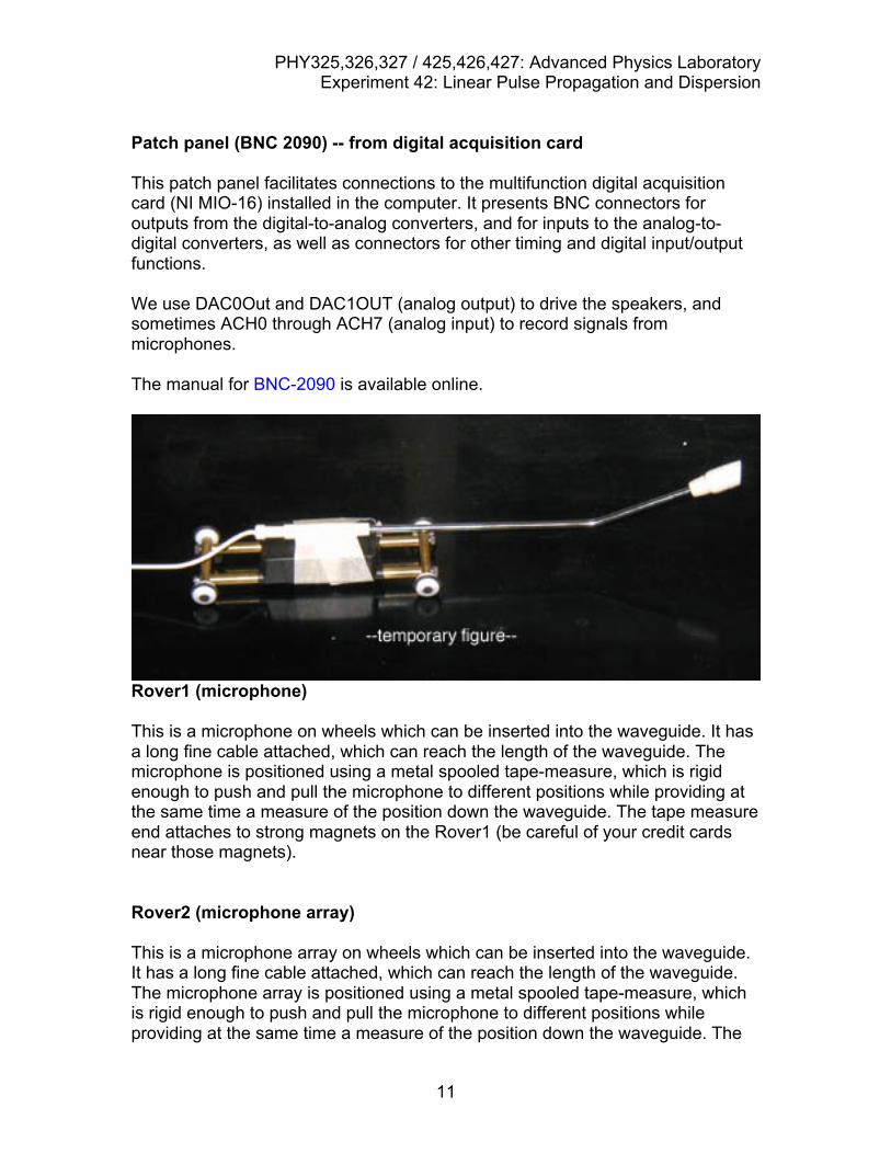
Patch panel (BNC 2090) -- from digital acquisition card This patch panel facilitates connections to the multifunction digital acquisition card (NI MIO-16) installed in the computer. It presents BNC connectors for outputs from the digital-to-analog converters, and for inputs to the analog-to-digital converters, as well as connectors for other timing and digital input/output functions. We use DAC0Out and DAC1OUT (analog output) to drive the speakers, and sometimes ACH0 through ACH7 (analog input) to record signals from microphones. The manual for BNC-2090 is available online.

Rover1 (microphone) This is a microphone on wheels which can be inserted into the waveguide. It has a long fine cable attached, which can reach the length of the waveguide. The microphone is positioned using a metal spooled tape-measure, which is rigid enough to push and pull the microphone to different positions while providing at the same time a measure of the position down the waveguide. The tape measure end attaches to strong magnets on the Rover1 (be careful of your credit cards near those magnets). Rover2 (microphone array) This is a microphone array on wheels which can be inserted into the waveguide. It has a long fine cable attached, which can reach the length of the waveguide. The microphone array is positioned using a metal spooled tape-measure, which is rigid enough to push and pull the microphone to different positions while providing at the same time a measure of the position down the waveguide. The


12

tape measure end attaches to strong magnets on the Rover (be careful of your credit cards near those magnets). The eight microphones of the array feed into eight input channels of the BNC-2090 patch panel; their signals are digitized by the multifunction data acquisition card of the computer, and displayed using special LabVIEW software, which makes a profile of the pressure variations along the array, and then shows the evolution of this profile, of the wave within the waveguide.


13

Section 4. Analysis. The goal of the quantitative analysis should be to compare your experimental data to the theory for the experiment. Use a fitting program which, if possible, gives you the Chi Squared of the fit, as well as uncertainty on your fitting parameters. Most importantly, you should compare the dispersion curves you found to the expected shape,

€

ω = cs kz2 +

2mπ /Lx( ) , where ω is the frequency, cs is the speed of sound, kz is the wave number, m is the mode number, and Lx is the size of the waveguide. Use the speed of sound and the size of the waveguide as fitting parameters, and compare to independent measurements or calculations. Group velocities should also be compared to theoretical expectations.


14

References Meykens et al., Am. J. Phys. 67, 5, (1999).

PHY325,326,327 / 425,426,427 Advanced Physics …phy326/lpp/PulsePropLab.pdf · Advanced Physics...

Documents

Transcript of PHY325,326,327 / 425,426,427 Advanced Physics …phy326/lpp/PulsePropLab.pdf · Advanced Physics...