
PHOTOVOLTAIC SYSTEMS IN HUNGARY AND...
124
1 UNIVERSITY OF PADUA FACULTY OF ENGINEERING MASTER'S DEGREE IN MECHANICAL ENGINEERING PHOTOVOLTAIC SYSTEMS IN HUNGARY AND ITALY: COMPARISON FOR A POWER PLANT Supervisor: Prof. Michele De Carli Author: Watutantrige Fernando Kay Co-Supervisor: Dr. Ákos Lakatos Mat. 1061372
Transcript of PHOTOVOLTAIC SYSTEMS IN HUNGARY AND...

1
UNIVERSITY OF PADUA FACULTY OF ENGINEERING
MASTER'S DEGREE IN MECHANICAL ENGINEERING
PHOTOVOLTAIC SYSTEMS IN HUNGARY AND ITALY: COMPARISON FOR A POWER PLANT
Supervisor: Prof. Michele De Carli Author: Watutantrige Fernando Kay
Co-Supervisor: Dr. Ákos Lakatos Mat. 1061372

2

3

1
1 Index 1
1.1 List of figures and tables 3
2 Abstract 9
3 Introduction 10
4 Photovoltaic Cells 11
4.1 Single crystal silicon 11
4.2 Czochralski process 14
4.3 Float Zone silicon process 15
4.4 Polycrystalline silicon 15
4.5 Ribbon silicon 17
4.6 Amorphous or thin film silicon 17
4.7 Multi-junction cells 19
4.7.1 Germanium substrate 19
4.7.2 Alloys semiconductors 21
4.7.3 Aluminium gallium arsenide 22
4.7.4 Indium gallium phosphide 23
4.7.5 Copper indium gallium arsenide 24
4.7.6 Cadmium telluride 26
5 Italian electric overview 27
5.1 Strong dependence on fossil fuels in the primary energy mix 27
5.2 Electrical energy demand in Italy in 2013 27
5.3 Distribution of consumption of energy 28
5.4 Focus on renewable sources 29
6 Hungarian electric overview 33
6.1 Introduction 33
6.2 Focus on renewable energies in Hungary 34
6.3 Overall view of the wind power energy in Hungary 37

2
6.4 Overall view of biomass, biogas and biofuels in Hungary 39
6.4.1 Biomass 40
6.4.2 Biogas 40
6.4.3 Biofuels 41
6.5 Overall view of hydropower in Hungary 42
6.5.1 Tiszalok 42
6.5.2 Kenyer 43
6.5.3 Ikervar 43
6.5.4 Kiskore 43
6.6 Overall view of geothermal energy in Hungary 44
6.7 Overall view of photovoltaic in Hungary 45
6.7.1 PV history in Hungary 46
7 Cost analysis 49
7.1 Overview of global trend 49
7.1.1 Forecasts of PV in Europe till 2018 52
7.2 Price trend for PV systems 55
7.2.1 LCOE parameter 60
7.2.2 Focus on Italian situation 62
7.2.3 Focus on Hungarian situation 68
8 Montalto di Castro 70
8.1 Principal data 72
8.2 Costs of the plant 72
9 Software SMA: Sunny Design 3 73
9.1 Introduction 73
9.2 Overview of the software 73
9.3 Purpose of the project 81
9.3.1 Venice 83
3
9.3.2 Budapest 85
9.4 Costs of the plant 88
9.5 Differences between Venice and Budapest 93
10 Software Photovoltaic Geographical Information System 100
10.1 Overview of the application 100
10.1.1 Ground measurements of solar irradiation 101
10.1.2 Solar radiation estimates from satellite 101
10.1.3 PVGIS Classic 102
10.1.4 PVGIS-CMSAF 102
10.2 Purpose of the project 103
10.3 Venice 104
10.3.1 Crystalline silicon technology 92 105
10.3.2 CIS technology 93 106
10.3.3 CdTe technology 95 110
10.4 Budapest 97 110
10.4.1 Crystalline silicon technology 98 111
10.4.2 CIS technology 99 112
10.4.3 CdTe technology 101 114
10.5 Differences between Venice and Budapest 102 116
11 Conclusions 104 119
12 References 107 121
1.1 List of figures and tables
Figure 1 Operation of a Photovoltaic Cell 12
Figure 2 Regular arrangement of silicon atoms in single-crystalline silicon and cell layered structure
13
Figure 3 Single crystalline in circular or semi-square solar cells 13

4
Figure 4 cylindrical section cut off to make wafers 15
Figure 5 Slab of multicrystalline silicon after growth 16
Figure 6 Boundary between two crystal grains 16
Figure 7 A 10 x 10 cm2 multicrystalline wafer 17
Figure 8 monocrystalline EPI-ready germanium wafers 20
Figure 9 The crystal structure of aluminium gallium arsenide 22
Figure 10 Cell's bottom indium gallium arsenide layer 23
Figure 11 Wavelength sensitivity of triple-junction cell for the InGaP, GaAs and InGaAs parts of the structure
24
Figure 12 Thin film of flexible CIGS 25
Figure 13 CIGS photovoltaic cell structure 25
Figure 14 Cross-section of a CdTe thin film solar cell and CdTe photovoltaic array 26
Figure 15 Consumption of electric energy in Italy 27
Figure 16 Power and number of photvoltaics plants 31
Figure 17 Regional distribution about power plants 32
Figure 18 Hungary’s primary energy use in 2012 (IEA) 33
Figure 19 Renewable energy potential in Hungary 35
Figure 20 Ratio of renewable energies (2010) 35
Figure 21 Ratio of renewable energies (2020) 36
Figure 22 Cumulate and yearly installed wind capacity in Hungary between 2000 and 2011 37
Figure 23 Wind speed on 75m above surface Country-side 38
Figure 24 Specific wind performance (W/m2) on 75m above surface Country-side wind potential on 75m
38
Figure 25 Expected generation wind power in next years 39
Figure 26 Tiszalok hydropower plant 42
Figure 27 Kenyer hydropower plant 43
Figure 28 Ikervar hydropower plant 43
Figure 29 Kiskore hydropower plant 44
Figure 30 Geothermal resource 45
5
Figure 31 Wellhead Temperature Regions of Water Wells areas 45
Figure 32 First PV installation in Hungary 1975 48
Figure 33 10 kWp grid connected PV systems 48
Figure 34 Global cumulated installed capacity 49
Figure 35 Global installed capacity 50
Figure 36 Installed capacity in Europe 51
Figure 37 Segmentation of PV market in Europe 52
Figure 38 Forecasts of the installed capacity in Europe 53
Figure 39 Forecasts of the cumulated installed capacity in Europe 53
Figure 40 Target for 2020 of cumulated installed capacity in Europe 54
Figure 41 Prices fall of modules from 1979 55
Figure 42 Prices of modules in the last years 56
Figure 43 Comparison of prices of modules between Europe and United States 56
Figure 44 Shared price of module 57
Figure 45 Inverters efficiency, cost and reliability 58
Figure 46 Shared price of a PV plant 59
Figure 47 Price forecasts for a PV plant 60
Figure 48 LCOE values for Europe 61
Figure 49 Photovoltaic convenience in Europe 62
Figure 50 Forecasts for cumulated installed capacity in Hungary 70
Figure 51 View of the Montalto di Castro Power Plants 71
Figure 52 First secton of Sunny Design 3 75
Figure 53 Second secton of Sunny Design 3 76
Figure 54 Third secton of Sunny Design 3 77
Figure 55 Fourth secton of Sunny Design 3 78
Figure 56 Fifth secton of Sunny Design 3 79
Figure 57 Sixth secton of Sunny Design 3 80
Figure 58 Sevent secton of Sunny Design 3 81
6
Figure 59 AC active power for Venice 83
Figure 60 Annual energy yield for Venice 84
Figure 61 Performance ratio for Venice 85
Figure 62 Specific energy yield for Venice 85
Figure 63 AC active power for Budapest 85
Figure 64 Annual energy yield for Budapest 86
Figure 65 Performance ratio for Budapest 87
Figure 66 Specific energy yield for Budapest 87
Figure 67 Payback time for Hungarian plants 92
Figure 68 Payback time for Hungarian plants 93
Figure 69 Average ambient temperature for Venice 94
Figure 70 Average ambient temperature for Budapest 94
Figure 71 Average global radiation for Venice 94
Figure 72 Average global radiation for Budapest 95
Figure 73 Angle of incidence during the year 97
Figure 74 Photovoltaic Geographical Information System web application 100
Figure 75 Outline horizon for sun path for winter and summer solstice in Venice 104
Figure 76 Daily in-plane radiation for 45° in Venice 104
Figure 77 Monthly in-plane radiation for 45° in Venice 104
Figure 78 Daily energy average output for 45° in Venice (silicon crystalline) 106
Figure 79 Monthly energy average output for 45° in Venice (silicon crystalline) 106
Figure 80 Daily energy average output for 45° in Venice (CIS) 108
Figure 81 Monthly energy average output for 45° in Venice (CIS) 108
Figure 82 Daily energy average output for 45° in Venice (CdTe) 109
Figure 83 Monthly energy average output for 45° in Venice (CdTe) 110
Figure 84 Outline horizon for sun path for winter and summer solstice in Budapest 110
Figure 85 Daily in-plane radiation for 45° in Budapest 110
Figure 86 Monthly in-plane radiation for 45° in Budapest 111

7
Figure 87 Daily energy average output for 45° in Budapest (silicon crystalline) 112
Figure 88 Monthly energy average output for 45° in Budapest (silicon crystalline) 112
Figure 89 Daily energy average output for 45° in Budapest (CIS) 113
Figure 90 Monthly energy average output for 45° in Budapest (CIS) 116
Figure 91 Daily energy average output for 45° in Budapest (CdTe) 115
Figure 92 Monthly energy average output for 45° in Budapest (CdTe) 115
Table 1 Section from the periodic table with more common semiconductor material in blue 21
Table 2 Italian consumption of electric energy in 2012 and 2013 28
Table 3 Italian production of electric energy in 2012 and 2013 29
Table 4 Renewable sources (2013, per region 31
Table 5 Hungary's fossil fuel resources 34
Table 6 Production and share of renewable energy in total energy demand 36
Table 7 Estimated amount of the available solid biomass for energy recovery 40
Table 8 Biomasses potential 41
Table 9 Installed and cumulated capacity in 2012 in Hungary 46
Table 10 Italian Fit for rooftop and grounded PV plant 66
Table 11 Italian Fit for concentrating and innovative PV plant 66
Table 12 Italian retail electricity and gas prices 68
Table 13 Hungarian Fit 68
Table 14 Hungarian retail electricity and gas prices 70
Table 15 Data for SMA Sunny Design project 81
Table 16 Data for alternatives in SMA Sunny Design 82
Table 17 Active power ratio for various alternatives 86
Table 18 Sum of costs for Italian plant 89
Table 19 Sum of costs for Hungarian plant 91
Table 20 Sum of payback time period for each alternative 93
Table 21 Performance ratio for various alternatives 96

8
Table 22 Best mounting angle for different cities 97
Table 23 Results for crystalline silicon pv system in Venice 105
Table 24 Results for CIS pv system in Venice 107
Table 25 Results for CdTe pv system in Venice 108
Table 26 Results for crystalline silicon pv system in Budapest 111
Table 27 Results for CIS pv system in Budapest 113
Table 28 Results for CdTe pv system in Budapest 114
Table 29 Comparison between Venice and Budapest irradiation (KWh/m2) 116
Table 30 Comparison between Venice and Budapest losses due to temperature and low irradiation
116
Table 31 Comparison between Venice and Budapest combined PV system losses 117
Table 32 Results for Silicon Crystalline pv system in Budapest with 35° angle 117

9
2 Abstract
The work shows a rapid view of the types of photovoltaic cells and their functioning. We
considered the most common cells, like single crystal silicon (mono), polycrystal silicon (poly),
amorphous silicon and some other alloys like Cadmium Tellurite (CdTe) and Copper Indium
Gallium Selenide (CIGS).
Then we reported the Italian and Hungarian electric overall, showing graphics about national
production and consumption. We displayed the shared quota for each type of electric resource,
focusing on renewable sources.
After that we analyzed the cost of photovoltaic plants, pointing out trends, forecasts and prices for
global, European, Italian and Hungarian market.
Using the software Sunny Design 3 we estimated the principal parameters for a photovoltaic
power plant with the same capacity of Montalto di Castro plant. We showed the performance
ratio and the annual energy yield for Venice and Budapest, considering four different alternatives
of PV modules for each city. Then we assessed the total costs of investment and the annual fixed
costs. Thus with the help of the software Matlab we implemented a script to estimate the revenue
from feeding the grid taking into account the actual Fits and calculating the payback period for
each station.
With another web application, Photovoltaic Geographical Information System, we estimated again
the annual energy yield in the two cities for 3 types of PV module.
The comparison of the PV systems in Hungary and Italy through different software and the data
obtained confirm that Italy is more advanced in the field and that the Italian Government
promotes the use of renewable energies more than Hungary.
10
3 Introduction
The Sun can satisfy all our needs if we learn to benefit with intelligence the energy that constantly
irradiates the Earth. It has shone in the sky for less than 5 billion years and, however, it is
estimated that it has reached just half of its existence. During the last year the sun radiated energy
towards the earth four thousand times and more than the entire world population consumption. It
would be foolish not to take advantage of that, given the technological means available,
considering that this energy source is free, clean and inexhaustible and can even free us from
dependence on oil and other alternative unsafe and contaminant energy sources.
Oil price is higher and higher, and pollution is less sustainable, thus making renewable alternative
energy sources an indispensable necessity. This energy can be used directly or converted into
electricity. Appropriately treated and controlled, it is possible to sell the energy produced and feed
the grid following national standards and rules. Economic incentives and the enormous progress of
electronic technology allow the use of photovoltaic systems with sustainable costs. Equipment for
direct connection on the net allows to take advantage of government incentives on the total
energy produced. An increasing interest in the use of inverters without transformers, for direct
connection to the network of photovoltaic systems, is growing, due to cost reductions and high
returns.
The choice of a photovoltaic solution represents an investment of sure and easily calculable
returns thanks to financing schemes provided by different national laws.
11
4 Photovoltaic cells
At present, most commercial photovoltaic cells are manufactured from silicon, which is the same
material as sand. In this case, however, silicon is extremely pure. Other exotic materials like
gallium arsenide are just at the beginning of the use in this field.
The four general types of silicon photovoltaic cells are:
Single-crystal silicon
Polycrystal silicon (also known as multicrystal silicon)
Ribbon silicon
Amorphous silicon (abbreviated as "aSi," also known as thin film silicon).
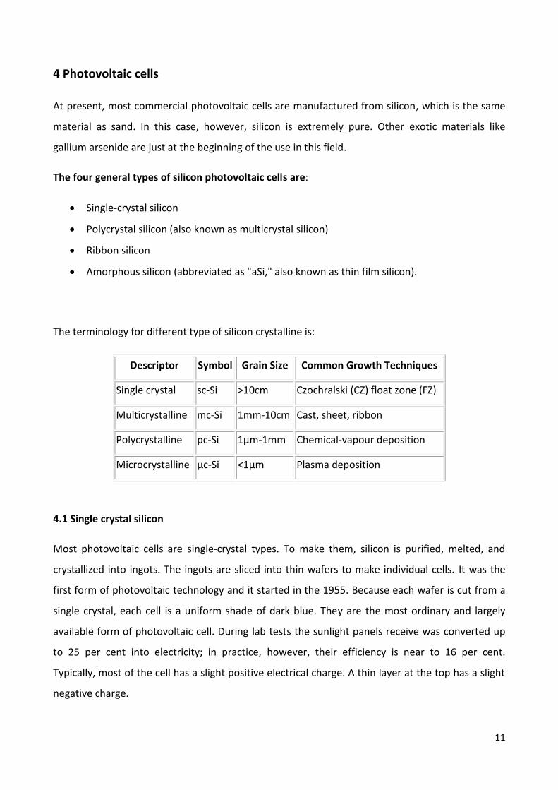
The terminology for different type of silicon crystalline is:
Descriptor Symbol Grain Size Common Growth Techniques
Single crystal sc-Si >10cm Czochralski (CZ) float zone (FZ)
Multicrystalline mc-Si 1mm-10cm Cast, sheet, ribbon
Polycrystalline pc-Si 1µm-1mm Chemical-vapour deposition
Microcrystalline µc-Si <1µm Plasma deposition
4.1 Single crystal silicon
Most photovoltaic cells are single-crystal types. To make them, silicon is purified, melted, and
crystallized into ingots. The ingots are sliced into thin wafers to make individual cells. It was the
first form of photovoltaic technology and it started in the 1955. Because each wafer is cut from a
single crystal, each cell is a uniform shade of dark blue. They are the most ordinary and largely
available form of photovoltaic cell. During lab tests the sunlight panels receive was converted up
to 25 per cent into electricity; in practice, however, their efficiency is near to 16 per cent.
Typically, most of the cell has a slight positive electrical charge. A thin layer at the top has a slight
negative charge.
12
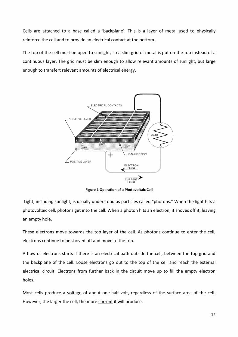
Cells are attached to a base called a ‘backplane’. This is a layer of metal used to physically
reinforce the cell and to provide an electrical contact at the bottom.
The top of the cell must be open to sunlight, so a slim grid of metal is put on the top instead of a
continuous layer. The grid must be slim enough to allow relevant amounts of sunlight, but large
enough to transfert relevant amounts of electrical energy.
Figure 1 Operation of a Photovoltaic Cell
Light, including sunlight, is usually understood as particles called "photons." When the light hits a
photovoltaic cell, photons get into the cell. When a photon hits an electron, it shoves off it, leaving
an empty hole.
These electrons move towards the top layer of the cell. As photons continue to enter the cell,
electrons continue to be shoved off and move to the top.
A flow of electrons starts if there is an electrical path outside the cell, between the top grid and
the backplane of the cell. Loose electrons go out to the top of the cell and reach the external
electrical circuit. Electrons from further back in the circuit move up to fill the empty electron
holes.
Most cells produce a voltage of about one-half volt, regardless of the surface area of the cell.
However, the larger the cell, the more current it will produce.

13
The cell is inside a circuit with some resistance, and that affects current and voltage. The amount
of available light influences current production. The temperature of the cell influences its voltage.
Having the knowledge about the electrical performance characteristics of a photovoltaic power
supply is very important.
Single-crystalline wafers usually have better material characteristics but their cost is higher.
Crystalline silicon has an ordered crystal structure, in which every atom stays in a determined
position. Crystalline silicon shows predictable and uniform behaviour, but, due to the slow and
precise manufacturing processes required, it is also the most expensive type of silicon.
Figure 2 regular arrangement of silicon atoms in single-crystalline silicon and cell layered structure
The proper arrangement of silicon atoms in single-crystalline silicon causes a sharp band structure.
Each silicon atom has four electrons in the external shell. Pairs of electrons from adjacent atoms
are shared. In this way each atom shares four bonds with close atoms.
Figure 3 Single crystalline in circular or semi-square solar cells
14
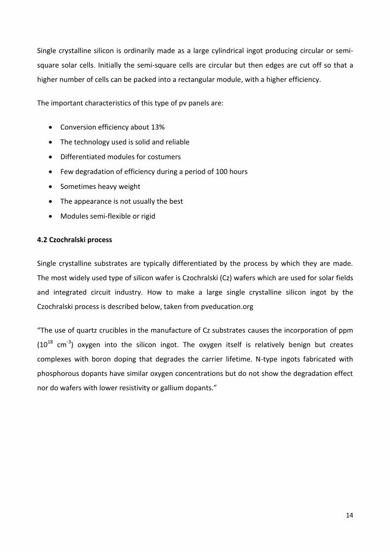
Single crystalline silicon is ordinarily made as a large cylindrical ingot producing circular or semi-
square solar cells. Initially the semi-square cells are circular but then edges are cut off so that a
higher number of cells can be packed into a rectangular module, with a higher efficiency.
The important characteristics of this type of pv panels are:
Conversion efficiency about 13%
The technology used is solid and reliable
Differentiated modules for costumers
Few degradation of efficiency during a period of 100 hours
Sometimes heavy weight
The appearance is not usually the best
Modules semi-flexible or rigid
4.2 Czochralski process
Single crystalline substrates are typically differentiated by the process by which they are made.
The most widely used type of silicon wafer is Czochralski (Cz) wafers which are used for solar fields
and integrated circuit industry. How to make a large single crystalline silicon ingot by the
Czochralski process is described below, taken from pveducation.org
“The use of quartz crucibles in the manufacture of Cz substrates causes the incorporation of ppm
(1018 cm-3) oxygen into the silicon ingot. The oxygen itself is relatively benign but creates
complexes with boron doping that degrades the carrier lifetime. N-type ingots fabricated with
phosphorous dopants have similar oxygen concentrations but do not show the degradation effect
nor do wafers with lower resistivity or gallium dopants.”
15
Figure 4 cylindrical section cut off to make wafers
4.3 Float Zone Silicon process
The CZ process is widely used for commercial substrates, but it has some disadvantages for high
efficiency laboratory or niche market solar cells. CZ wafers hold inside a large amount of oxygen in
the silicon wafer. Oxygen impurities decrease the lifetime in the solar cell, thus reducing the
voltage, current and efficiency. Furthermore, the oxygen and complexes of the oxygen with other
elements may become active at higher temperatures, making the wafers sensitive to high
temperature processing. To remove these problems, Float Zone (FZ) wafers can be used.
In this process, a molten region is slowly passed along a rod or bar of silicon. Impurities in the
molten region are incline to remain in the molten region rather than being integrated into the
solidified region, thus permitting a very pure single crystal region after the molten region has
passed. Due to the difficulty to grow large diameter ingots and the very high cost, FZ wafers are
usually used for laboratory cells and rarely used in commercial production.
4.4 Polycrystalline silicon
Polycrystalline cells are manufactured and work in a similar way. The lower cost of the silicon used
is the main difference. Techniques for the production of multicrystalline silicon are simpler than
for single crystal material. However, the material quality of multicrystalline material is lower than
that of single crystalline material. This is due to the presence of grain boundaries. Grain
boundaries introduce high localized regions of recombination due to the introduction of extra
defect energy levels into the band gap, and this reduces the overall minority carrier lifetime from

16
the material. In addition, grain boundaries reduce solar cell performance by blocking carrier flows
and supplying shunting tracks for current flow across the p-n junction. Polycrystalline cell
manufacturers state that the low cost of the material produces more benefits, even if the
efficiency is lower.
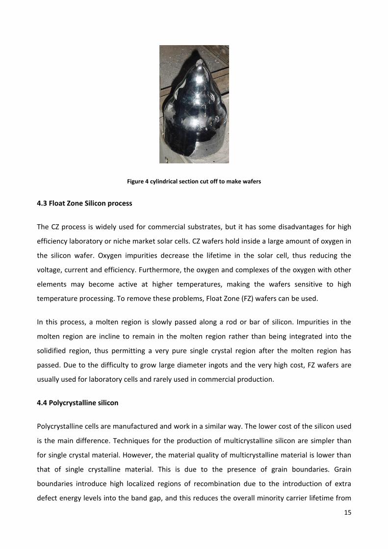
Figure 5 Slab of multicrystalline silicon after growth
Grain sizes must be on the order of at least a few millimeters to avoid significant recombination
losses at grain boundaries. This allows also single grains to extend from front to back of the cell,
providing less resistance to carrier flow and generally decreasing the length of grain boundaries
per unit of cell. For these reasons multicrystalline material is widely used for commercial solar cell
production.
Figure 6 boundary between two crystal grains

17
At the boundary between two crystal grains, the bonds are strained, degrading the electronic
properties.
Figure 7 A 10 x 10 cm2 multicrystalline wafer
The wafer has been textured so that grains of different orientation show up as light and dark.
4.5 Ribbon silicon (polycrystal)
The process of ribbon-type photovoltaic cells, in opposition to the crystalline type which is made
from an ingot, is to grow a ribbon from the molten silicon. These cells operate in the same way as
single and polycrystal cells.
The anti-reflective coating used on most ribbon silicon cells gives them a prismatic rainbow
appearance.
4.6 Amorphous or thin film silicon
The previous three types of silicon used for photovoltaic cells have a distinct crystal structure. The
amorphous silicon has no structure. Amorphous silicon is usually called thin film silicon and
sometimes abbreviated "aSi".
Amorphous silicon units are made by depositing very thin layers of vaporized silicon in a vacuum
onto a support of glass, plastic, or metal.

18
Amorphous silicon cells are produced in a variety of colours.
They are made up in long rectangular "strip cells” because their size can be several square yards.
These are connected in series to form "modules."
Multiple layers can be deposited because the layers of silicon allow some light to pass through.
The photovoltaic cell can produce more electricity because of multiple layers.
Each layer can be set to receive a particular band of light wavelength.
The performance of amorphous silicon cells can achieve not more than 15% upon initial exposure
to sunlight. This drop takes around six weeks. Manufacturers usually publish post-exposure
performance data, so if the module has not been exposed to sunlight, its performance will exceed
specifications at first.
The efficiency of amorphous silicon photovoltaic modules is less than half that of the other three
technologies. This technology has the potential of being much less expensive to produce than
crystalline silicon technology.
For this reason, there are a lot of investigations to improve amorphous silicon performance and
producing processes. This type of PV module suits rural electrification, solar home system, grid
connected system, solar water pump system or cathodic protection.
The important characteristics of this type of pv panels are:
Make multi-substrates (also flexible)
Good appearance
Possibility to create pv panels which can substitute architectural elements (tiles, sheets)
Degradation of the efficiency in the first 100 hours of 10-15%
After the first degradation efficiency about 6%
Double space for the same electricity generation compared to Si crystalline
19
4.7 Multi-junction cells
Cells made from multiple materials have multiple band gaps. So, it will respond to multiple light
wavelengths and some of the energy that would otherwise be lost to relaxation as described
above, can be captured and converted.
For example, if one had a cell with two band gaps in it, one tuned to red light and the other to
green, then the extra energy in green, cyan and blue light would be lost only to the band gap of
the green-sensitive material, while the energy of the red, yellow and orange would be lost only to
the band gap of the red-sensitive material. Making similar analysis to those executed for single-
band gap modules, it can be proved that the perfect band gaps for a two-gap module are at 1.1 eV
and 1.8 eV.
Light of a particular wavelength does not interact at all with materials that are not a multiple of
that wavelength. This means that one can do a multi-junction cell by making layers of the different
materials on top of each other. Usually the shortest wavelength layer is put on the "top" and other
increasing through the body of the cell. As the photons have to cross the cell to achieve the
correct layer to be absorbed, to collect the electrons generated at each layer we need to use
transparent conductors.
Usually alloys are used for the multi-junctions cells. They provide more efficiency and in this way
bandgaps can be modified. There are lots of types of alloys used for the photovoltaic parks, and
they are used not only in the terrestrial field, but also in the space. An example of alloy is with
Germanium.
4.7.1 Germanium substrate
Germanium wafers offer high strength at minimal thickness and concur busily to the overall cell
performance. Germanium substrates are enforced in III-V triple-junction solar cells, a solution that
nowadays is widely used to power virtually all satellites placed in orbit, as well as in terrestrial
solar cells to power photovoltaic plant systems. There is only one big supplier of Germanium pv
and it is Umicore (USA).
Thanks to the closely matching thermal and crystallographic properties of Germanium and Gallium
Arsenide, Germanium substrates provide an interesting alternative for the epitaxial growth and

20
layer transfer of III-V compounds. For proper nucleation, the wafers are precisely cut off along the
appropriate direction and have been cleaned.
Umicore is one of the best supplier for EPI-ready, dislocation free Germanium substrates for III-V
multi-junction solar cells for space applications. Germanium technology has gradually replaced Si-
based solutions. Germanium is the preferred substrate because it provides high strength at
minimal thickness also with hard radiation. Advanced triple junction solar cells with Germanium
substrates offer the best end-of-life performance over weight ratio.
The high-efficiency solar cells on Germanium can also provide good application in the field of
terrestrial photovoltaic, whereby the cells are integrated in a concentrator system based on
refractive or reflective optics. Under concentration, the most fully-developed solar cells on
Germanium have a conversion efficiency of 41 % and open the way for sustainable energy
generation and lower cost.
Figure 8 monocrystalline EPI-ready germanium wafers
Germanium offers an interesting alternative to silicon. It has larger excitonic Bohr radius
compared to silicon because it has smaller electron effective mass and a larger dielectric constant.
This results in a more prominent quantum confinement effect thus allowing the possibility of
engineering the effective band gap over a large range. More importantly, wafers can be fabricated
below 400 °C whereas Si nanocrystals are typically fabricated at much higher temperature ~1100
°C. The low temperature growth of Ge nanocrystals offers significant advantages for processing
compatibility and for reduced processing costs.
21
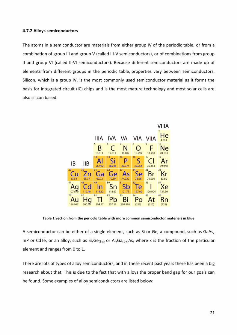
4.7.2 Alloys semiconductors
The atoms in a semiconductor are materials from either group IV of the periodic table, or from a
combination of group III and group V (called III-V semiconductors), or of combinations from group
II and group VI (called II-VI semiconductors). Because different semiconductors are made up of
elements from different groups in the periodic table, properties vary between semiconductors.
Silicon, which is a group IV, is the most commonly used semiconductor material as it forms the
basis for integrated circuit (IC) chips and is the most mature technology and most solar cells are
also silicon based.
Table 1 Section from the periodic table with more common semiconductor materials in blue
A semiconductor can be either of a single element, such as Si or Ge, a compound, such as GaAs,
InP or CdTe, or an alloy, such as SixGe(1-x) or AlxGa(1-x)As, where x is the fraction of the particular
element and ranges from 0 to 1.
There are lots of types of alloy semiconductors, and in these recent past years there has been a big
research about that. This is due to the fact that with alloys the proper band gap for our goals can
be found. Some examples of alloy semiconductors are listed below:

22
4.7.3 Aluminium gallium arsenide (AlxGa1-xAs)
Aluminium gallium AlxGa1-xAs is a semiconductor material with very nearly the same lattice
constant as GaAs, but with a larger band gap. The x in the formula above is a number between 0
and 1 (this indicates an arbitrary alloy between GaAs and AlAs). The band gap varies between 1.42
eV (GaAs) and 2.16 eV (AlAs). For x < 0.4, the band gap is direct. The formula AlGaAs should be
considered an abbreviated form of the above, rather than any particular ratio. Aluminium gallium
arsenide is used as a barrier material in GaAs based heterostructure devices. The AlGaAs layer
confines the electrons to a gallium arsenide region (QWIP). AlGaAs with composition close to AlAs
is almost transparent to sunlight. It is used in GaAs/AlGaAs solar cells.
Figure 9 The crystal structure of aluminium gallium arsenide
The toxicology of AlGaAs has not been fully investigated. Dust is an irritant to skin, eyes and lungs.
The environment, health and safety aspects of aluminuim gallium arsenide sources and industrial
hygiene monitoring studies of standard MOVPE sources have been recently reported in a review.
Indium gallium arsenide is a ternary alloy of indium, gallium and arsenic. It’s a well-developed
material.
The band gap energy of GaInAs can be determined from the peak in the photoluminescence
spectrum, provided that the total impurity and defect concentration is less than 5×1016cm-3. The
band gap energy depends on temperature and increases as the temperature decreases for both n-
23
type and p-type samples. The band gap energy at room temperature is 0.75 eV and lies between
that of Ge and Si.
Single crystal epitaxial films of InGaAs can be deposited on a single crystal substrate of III-V
semiconductor having a lattice parameter close to that of the specific gallium indium arsenide
alloy to be synthesized. Three substrates can be used: GaAs, InAs and InP. A good match between
the lattice constants of the film and substrate is required to maintain single crystal properties and
this limitation permits small variations in composition on the order of a few per cent. Therefore
the properties of epitaxial films of GaInAs alloys grown on GaAs are very similar to GaAs and those
grown on InAs are very similar to InAs, because lattice mismatch strain does not generally permit
significant deviation of the composition from the pure binary substrate. Ga0.47In0.53As is the
alloy whose lattice parameter matches that of InP at 295 K.
GaInAs lattice-matched to InP is a semiconductor with properties quite different from GaAs, InAs
or InP. It has an energy band gap of 0.75 eV, an electron effective mass of 0.041 and an electron
mobility close to 10,000 cm2·V−1·s−1 at room temperature, all of which are more favorable for
many electronic and photonic device applications when compared to GaAs, InP or even Si.
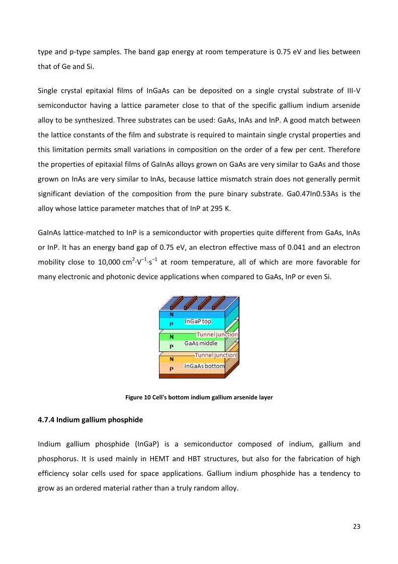
Figure 10 Cell's bottom indium gallium arsenide layer
4.7.4 Indium gallium phosphide
Indium gallium phosphide (InGaP) is a semiconductor composed of indium, gallium and
phosphorus. It is used mainly in HEMT and HBT structures, but also for the fabrication of high
efficiency solar cells used for space applications. Gallium indium phosphide has a tendency to
grow as an ordered material rather than a truly random alloy.

24
Other applications of gallium indium phosphide include semiconductor lasers such as vertical-
cavity surface-emitting laser for plastic optical fibers and high energy junction on double and triple
junction photovoltaic cells.
Figure 11 Wavelength sensitivity of triple-junction cell for the InGaP, GaAs and InGaAs parts of the structure
The basic structure of the latest triple-junction compound solar cell uses proprietary Sharp
technology that enables efficient stacking of the three photo-absorption layers, with an InGaP
(indium gallium phosphide) top layer, GaAs (gallium arsenide) middle layer and InGaAs (indium
gallium arsenide) bottom layer, separated by tunnel junctions.
4.7.5 Copper indium gallium selenide
CIGS is a I-III-VI2 compound semiconductor material composed of copper, indium, gallium, and
selenium. The material is a solid solution of copper indium selenide and copper gallium selenide,
with a chemical formula of CuInxGa(1-x)Se2, where the value of x can vary from 1 (pure copper
indium selenide) to 0 (pure copper gallium selenide).
The bandgap varies continuously with x from about 1.0 eV (for copper indium selenide) to about
1.7 eV (for copper gallium selenide).
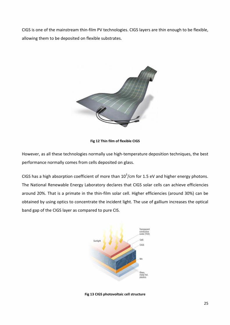
A copper indium gallium selenide solar cell is a thin film solar cell that is manufactured by
depositing a thin layer of copper, indium, gallium and selenide on glass or plastic backing, along
with electrodes on the front and back to collect current. Because the material has a high
absorption coefficient and strongly absorbs sunlight, a much thinner film is required than that of
other semiconductor materials.
25
CIGS is one of the mainstream thin-film PV technologies. CIGS layers are thin enough to be flexible,
allowing them to be deposited on flexible substrates.
Fig 12 Thin film of flexible CIGS
However, as all these technologies normally use high-temperature deposition techniques, the best
performance normally comes from cells deposited on glass.
CIGS has a high absorption coefficient of more than 105/cm for 1.5 eV and higher energy photons.
The National Renewable Energy Laboratory declares that CIGS solar cells can achieve efficiencies
around 20%. That is a primate in the thin-film solar cell. Higher efficiencies (around 30%) can be
obtained by using optics to concentrate the incident light. The use of gallium increases the optical
band gap of the CIGS layer as compared to pure CIS.
Fig 13 CIGS photovoltaic cell structure
26
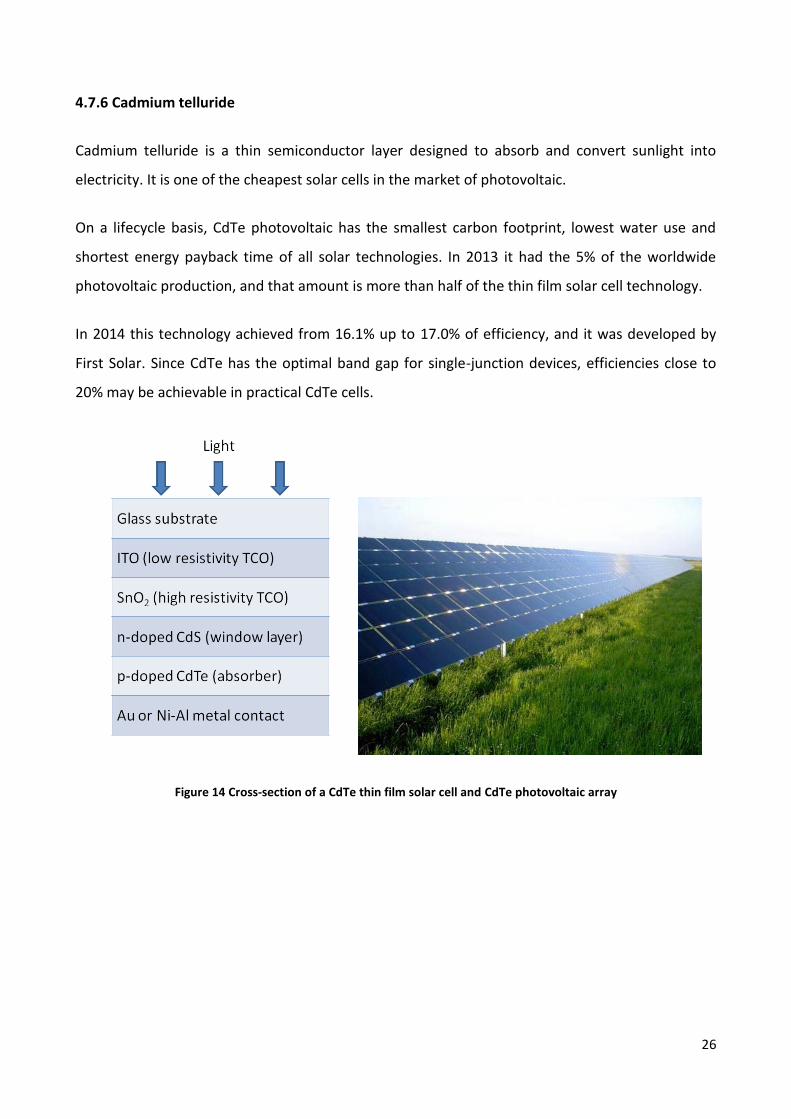
4.7.6 Cadmium telluride
Cadmium telluride is a thin semiconductor layer designed to absorb and convert sunlight into
electricity. It is one of the cheapest solar cells in the market of photovoltaic.
On a lifecycle basis, CdTe photovoltaic has the smallest carbon footprint, lowest water use and
shortest energy payback time of all solar technologies. In 2013 it had the 5% of the worldwide
photovoltaic production, and that amount is more than half of the thin film solar cell technology.
In 2014 this technology achieved from 16.1% up to 17.0% of efficiency, and it was developed by
First Solar. Since CdTe has the optimal band gap for single-junction devices, efficiencies close to
20% may be achievable in practical CdTe cells.
Figure 14 Cross-section of a CdTe thin film solar cell and CdTe photovoltaic array
27
5 Italian electric overall
In Italy, the issue of energy supply is always of great interest because this country depends on
foreign imports for 83% of its primary energy needs.
5.1 The strong dependence on fossil fuels in the primary energy mix
In 2010, Italian gross demand of primary energy amounted to 2183.9 TWh (187.79 Mtep,). 82.7%
of the requirement was satisfied by fossil fuels: more specifically, oil covered 38.5% of the total,
natural gas 36.2% and coal 8%. The energy mix was completed by renewable sources (265.8 TWh,
12.2%), constituted mainly by hydroelectric power (67.6%), and by the net import of electricity
(113 TWh, 5.1%). In Italy, natural gas is widely employed in electricity production, the conversion
concerns roughly a third (36%) of the primary input, causing a greater dependence from this kind
of source compared to other European countries. Almost all the remaining consumption occurs in
the industrial sector (18.8%) and for heating of homes and commercial/service buildings (40.8%).
Regarding oil, only 5.5% is converted into electric power, while 54.7% is employed by the
transportation sector. Coal is mainly used to produce electricity (71.5%) and the residual part is
given to the industries. It is worth noting that 82% of the Italian primary energy supply comes
from imports, resulting in a strong dependence on foreign fossil fuels. The domestic production of
fossil fuels amounts to a total of 142 TWh; 56% of the domestic production consists of gas (80.1
TWh, 10.1% of the entire gross availability of natural gas) and 42% of oil (59.1 TWh, 7% of the total
amount); including the increasing contribution of renewable sources (246 TWh), the total internal
production constitutes 18% of the whole energy mix.
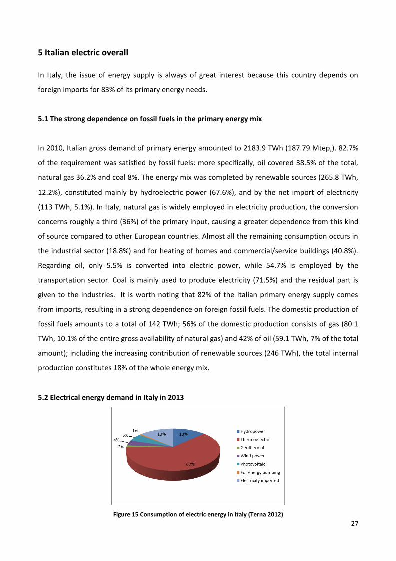
5.2 Electrical energy demand in Italy in 2013
Figure 15 Consumption of electric energy in Italy (Terna 2012)

28
In 2013 the demand of electric energy was 318.5 million KWh. The demand of energy was satisfied
by the 86.8 % from the national production, for an amount of 276.3 billion KWh, considering
pumping energy and auxiliaries. The remain amount (13.2%, 42.1 billion KWh) was covered from
the import from other countries, with a reduction of 2,2% previous year. The consumption of the
total electric energy in 2013 was 297.3 billion KWh.
5.3 Distribution of consumption of energy
In the industrial section the amount is 124.9 billion of KWh (42%). For the auxiliaries it is 99.8
billion KWh. For domestic uses 67 billion KWh and for agriculture 5.7 billion KWh.
There is an increment of the hydroelectric power (+24.7%) with 54.7 billion KWh. The production
from renewable sources (hydric, eolic, photovoltaic, geothermic and bioenergy) is increased about
21.5 %. There was a big increase for the photovoltaic energy (+14.5%) with an amount of 21.6
billion KWh. Also the eolic energy had an increase of +11.1% with an amount of 14.9 billion KWh.
For the bioenergy the increase was +36.9% with 17.1 billion KWh.
The production from the thermic sources was the 65.5 % of the total amount of the national
production. The most fuel used for the production is the natural gas with a 57.8 % of the total
amount.
Table 2 Italian consumption of electric energy in 2012 and 2013 (Terna 2013)

29
Table 3 Italian production of electric energy in 2012 and 2013 (Terna 2013)
5.4 Focus on renewable sources
Solar
Italy is one of the world’s largest producers of electricity from solar power with an installed
photovoltaic capacity of 17,968 MW at the end of 2013 and 603,196 plants in operation as at the
end of 2013.The total energy produced by solar power in 2013 was 21,299 GWh, about 6.7% of
the total electricity demand of 332.3 TWh. The installed photovoltaic capacity, compared to that
of the previous year, grew of 29% in 2012 and 9% in 2013.
As for December 2012, the installed capacity was approaching 17 GW, with such an important
production that several gas turbine power plants started to operate at half their potential during
the day. This field gave employment to about 100,000 people, especially in design and installation.
Wind energy
Best wind resources in Italy are located in the south, particularly the Apennine Mountains, on the
coast and in the major islands. Also the relatively large off-shore potential is located in the
southern coastal areas and islands. This means that a large share of non-programmable electricity
would be fed into the grid in such areas. Unfortunately, the power grid in these areas is poor for

30
historical reasons, since these areas are less densely populated and larger consumption centers
are located in the North.
Biomass
The current resources of biomasses, which derive principally from agricultural and forest residues,
firewood, livestock muck and the biodegradable portion of solid urban waste, can achieve not
more than 20-25 Mtoe/year. More quantities of raw material can be generated by renewing the
non-food agricultural sector and the forest sector, together with the recovery of abandoned agro-
wood territories, which extend for at least 2 million hectares.
Hydro
Since long time ago water energy has been the major national energy source in Italy and the
primary resource alternative to fossil fuel sources. There are more than 2000 hydroelectric power
plants mainly in the Alpine region, of which 300 have a production capacity of more than 10 MW.
The 80% of electricity is produced in large plants. The other 20% is covered with small and medium
plants under 10 MW, which were developed and added in recent years. The hydroelectric power
plants in 2007 achieved the 72% of the electricity production from renewable sources. However,
its potential has been fully exploited.
Geothermal
The geothermal potential is remarkable economically speaking. The high temperature resources
(>150° C) are gathered in the Apennines in Tuscany, Latium and Campania and on some volcanic
islands of the Tyrrhenian Sea. The medium and low temperature (< 150°C) sources instead can be
found on large areas of the national territory. The high-temperature resources are employed for
the production of electricity and direct uses, while the medium and low temperature resources
can be used mostly for heating systems.

31
Table 4 Renewable sources per region (Terna 2013, GWh)
Figure 16 Power and number of photvoltaics plants ( Terna 2012)
32
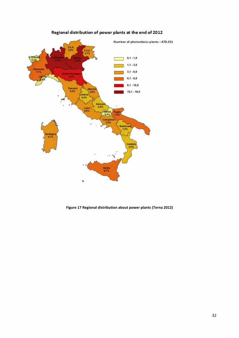
Figure 17 Regional distribution about power plants (Terna 2012)

33
6 Hungarian electric overall
6.1 Introduction
For Hungary the main electric power come from fossil fuels. In 2009 the amount was about 75% of
the total, and it comes from Russia, essentially through a single transport route (the Brotherhood
pipeline), which results in a vulnerable situation for Hungary in terms of the security of supply.
Figure 18 Hungary’s primary energy use 2012 (IEA)
The current Hungarian gas storage capacity exceeds 50 percent of the annual natural gas
consumption (5.8 billion m3). According to the requirements of the IEA and the EU, crude oil
and oil products are stored at a quantity equivalent to at least 90 days of consumption.
Renewable energy in final energy consumption was 6.6% in 2008 (7.4% in 2010 is foreseen by
the NREAP (national renewable energy action plan)). Hungary ranks in the lowest third among
EU member states (2008 EU-27 average: 10.3 percent) lagging behind even the countries of a
similar level of economic development (Bulgaria 9.4 percent, Czech Republic 7.2 percent, Poland
7.9 percent, Romania 20.4 percent and Slovakia 8.4 percent).
The reason is because neighbour countries have more favourable and better hydro energy
potential which is exploited very well, counter Hungary. On the basis of Directive
2009/28/EC14, this indicator should reach 13 percent in Hungary by 2020.
In terms of the utilization of renewable energy sources, Hungary has so far failed to make full
use of the available domestic potential. According to the findings of a survey conducted in

34
2005 and 2006 by the Renewable Energy Subcommittee of the Hungarian Academy of
Sciences, the theoretical annual renewable energy potential is around 720000 GWh, the full
exploitation of which can never be achieved.
Table 5 Hungary's fossil fuel resources
One of the most important sources in the past was coal. After 1960s the extraction of coal was
reduced gradually. It will be a good thing increasing the use of Hungarian coal, fulfilling
environmental requirements.
Sources of natural gas provide at least 3563 billion m3. However at the moment there are not
solutions for the extraction of it, so it is useless. If we consider just the working mining, the
volume that can be extracted is 56.6 billion m3 at 1 January 2008, ensuring supply for 21 years.
We can estimate the volume of gas that can be mined. Using the actual technology knowledge,
drilling of fifty wells a year, at least 30 percent of that industrial asset can be mined over the
forthcoming 30 years. That would cover over one-third (34.2 percent) of domestic demand.
In Hungary there was also the production of uranium, which took place near the village of
Kôvágószôlôs. From the uranium mined uranium oxide was produced. Subsequently it was
processed into fuel in the former Soviet Union. At the end of 1997 the mine was closed for
economic reason, so Hungary was no longer in the market of uranium. Since 2006, however,
the increase of market demand has spurred intensive search for uranium in Southwest Hungary
(Mecsek, Bátaszék, Dinnyeberki and Máriakéménd).
6.2 Focus on renewable energies in Hungary
Since the mid of 1990s in Hungary the mass media have started to support the use of renewable
energy. The price of oil and gas has increased rapidly, so renewable energy has become a valid

35
opportunity and alternative. Discussing about it, Hungary would have a lot of benefit from
renewable sources, especially in the agricultural production. Despite that, the cost of energy will
be much higher than normal sources, so it wouldn’t be a good investment and not economically
competitive.
After joining the European Union (2003) renewable energy utilization started to grow
intensively in Hungary. Before 2004 the energy coming from renewable source was only 0.5% of
the total amount. In 2009 it was 4.3%, so there was a good increasing. At present biomass
represents almost 80% and geothermal 8.2% of renewable energy use. Hungary is rich in
renewable energy sources. Pellets and other solid biomass are the most used resources in the
ratio of the renewable sources. The graphic underneath shows the distribution of renewable
sources.
Figure 19 Renewable energy potential in Hungary
Figure 20 Ratio of renewable energies (2010)

36
From this graphic we can see the distribution of green energy. Wood is the most used with an
amount of 40.74 Pj. After that there is a good amount of geothermal energy, which provides
4.23 Pj. For the moment solar energy has a really small amount in renewable energy, but it is
increasing very rapidly and it is taking significantly part of the amount in these years. Also hydro
energy has a small amount (0.7 PJ) and it is decreasing. Wind energy has been recently
introduced in Hungary and for the moment it is not much utilized.
The following table shows briefly the amount of production and share of renewable energy
in total energy demand:
Table 6 Production and share of renewable energy in total energy demand
In the next graphic we can see what Hungary wants to achieve in the 2020 for renewable energy.
Figure 21 Ratio of renewable energies (2020)

37
6.3 Overall view of wind power energy in Hungary
In 2010 the participation of the wind turbines in the total amount of renewable energy was about
5%. Based on surveys, the potential capacity of wind power in Hungary is much more than the
utilized power at the moment. According to the guideline of the government and the limitation of
the controllability of the electric system, for 2020 Hungary wants to achieve 740 MW from the
energy of wind turbine.
Figure 22 Cumulate and yearly installed wind capacity in Hungary between 2000 and 2011
The graphic shows how wind power is increasing year per year. In fact, almost 43% of the
territory allows a suitable economic utilization of wind power. In areas which are 75 m above sea
level, the annual average wind speed is above 5.5 m/s. In higher areas the wind is also faster, so
that more efficiency can be reached.

38
Figure 23 wind speed on 75m above surface Country-side
Figure 24 Specific wind performance (W/m2) on 75m above surface Country-side wind potential on 75m
39
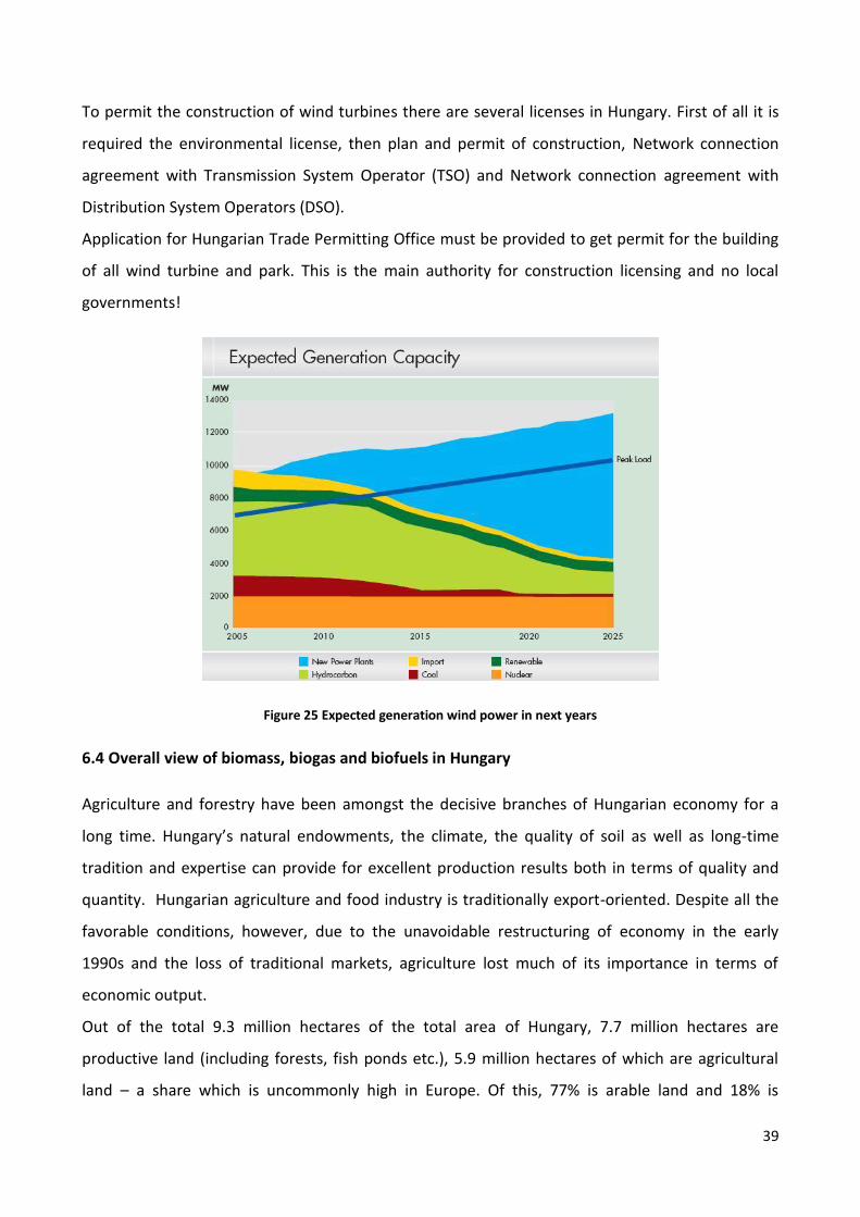
To permit the construction of wind turbines there are several licenses in Hungary. First of all it is
required the environmental license, then plan and permit of construction, Network connection
agreement with Transmission System Operator (TSO) and Network connection agreement with
Distribution System Operators (DSO).
Application for Hungarian Trade Permitting Office must be provided to get permit for the building
of all wind turbine and park. This is the main authority for construction licensing and no local
governments!
Figure 25 Expected generation wind power in next years
6.4 Overall view of biomass, biogas and biofuels in Hungary
Agriculture and forestry have been amongst the decisive branches of Hungarian economy for a
long time. Hungary’s natural endowments, the climate, the quality of soil as well as long-time
tradition and expertise can provide for excellent production results both in terms of quality and
quantity. Hungarian agriculture and food industry is traditionally export-oriented. Despite all the
favorable conditions, however, due to the unavoidable restructuring of economy in the early
1990s and the loss of traditional markets, agriculture lost much of its importance in terms of
economic output.
Out of the total 9.3 million hectares of the total area of Hungary, 7.7 million hectares are
productive land (including forests, fish ponds etc.), 5.9 million hectares of which are agricultural
land – a share which is uncommonly high in Europe. Of this, 77% is arable land and 18% is
40
grassland. Kitchen gardens, orchards and vineyards account for 5% of the agricultural land area.
For this reason Hungary possesses good agro-ecological conditions for a competitive production of
biomass. A lot of food can be produced and at the same time also a big biogas production
potential. Anyway, there are some limitations due to the competitiveness of the energy. Bioenergy
can primarily play a more important part in fulfilling local heating demands in the future, but
there is also an intent to place emphasis on the spread of small and medium-capacity combined
electricity and heat generating systems.
6.4.1 Biomass
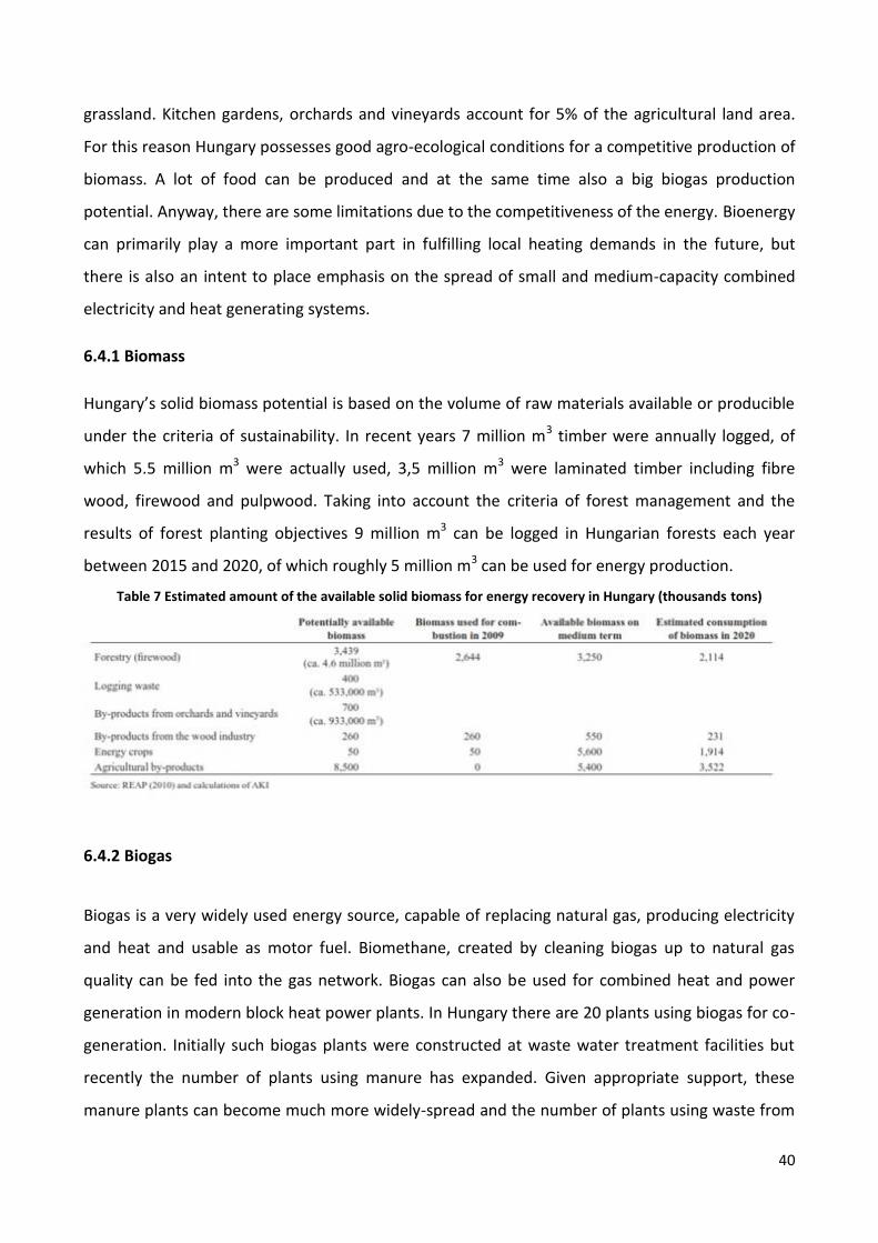
Hungary’s solid biomass potential is based on the volume of raw materials available or producible
under the criteria of sustainability. In recent years 7 million m3 timber were annually logged, of
which 5.5 million m3 were actually used, 3,5 million m3 were laminated timber including fibre
wood, firewood and pulpwood. Taking into account the criteria of forest management and the
results of forest planting objectives 9 million m3 can be logged in Hungarian forests each year
between 2015 and 2020, of which roughly 5 million m3 can be used for energy production.
Table 7 Estimated amount of the available solid biomass for energy recovery in Hungary (thousands tons)
6.4.2 Biogas
Biogas is a very widely used energy source, capable of replacing natural gas, producing electricity
and heat and usable as motor fuel. Biomethane, created by cleaning biogas up to natural gas
quality can be fed into the gas network. Biogas can also be used for combined heat and power
generation in modern block heat power plants. In Hungary there are 20 plants using biogas for co-
generation. Initially such biogas plants were constructed at waste water treatment facilities but
recently the number of plants using manure has expanded. Given appropriate support, these
manure plants can become much more widely-spread and the number of plants using waste from

41
the food industry can also considerably rise. This is underlined by the increasingly stricter
environmental regulations prohibiting the flushing of liquid manure into waters to reduce the
agricultural nitrate pollution of water.
6.4.3 Biofuels
Raw materials used for bioethanol production include plants with high sugar content (e.g. sugar
beet, sugarcane) or crops that can be converted to sugar (e.g. maize, wheat, potatoes with starch
etc., or trees, grasses, grain stalks, straw containing cellulose). Bioethanol production can be based
on a wide range of raw materials including existing agricultural by-products and waste. In Hungary
the main raw materials used in first generation bioethanol production are maize, wheat, Jerusalem
artichoke and sugar beet.
In addition several cultures are being tested (e.g. sweet sorghum). The technology of the near
future, however, is a second-generation bioethanol production based on cellulose, currently under
development. Its wider dissemination in factories is expected to take place after 2012-2015. In
terms of raw materials Hungary is in a favorable position to produce bioethanol. 6-7 million tons of
maize is annually harvested, of which increasingly less is used as fodder while the amount
exported and industrially processed is rising. Locally grown maize is available in much larger
quantities than the estimated demand in the near future. The volume of maize and cereal-based
ethanol can go up to 700-800,000 tons/year, exceeding the expected needs of Hungarian motor
fuel producers and sellers multiple times by 2020. To achieve this aim bioethanol plants must be
set up at a different rate than the current disappointing one.
Table 8 Biomasses potential

42
6.5 Overall view of hydropower in Hungary
In Hungary this type of energy is one of the oldest. It had a great role in the generation of energy
in past years. The strengths of this energy are that it is clean and renewable, and it has a good
efficiency of conversion. Choosing this type of energy, we can reduce drastically the greenhouse
effect, because we would not produce CO2. However in Hungary there are just small opportunities
to have this type of plants due to the fact that there are just small rivers’ falls. Actually in Hungary
there are 11 hydropower plants plus 6 smaller hydropower plants.
At the beginning of the 20th century some watermills were converted to smaller hydropower
plants.
The theoretical potential of electricity generation is around 7500 GWh/year.
Hydropower potential in Hungary is limited to 3 larger power plants, and several small power
hydropower plants.
The main plants are:
Tiszalök
Kenyer
Ikervar
Kisköre
6.5.1 Tiszalok
This is the biggest hydropower plant.
Figure 26 Tiszalok hydropower plant
43
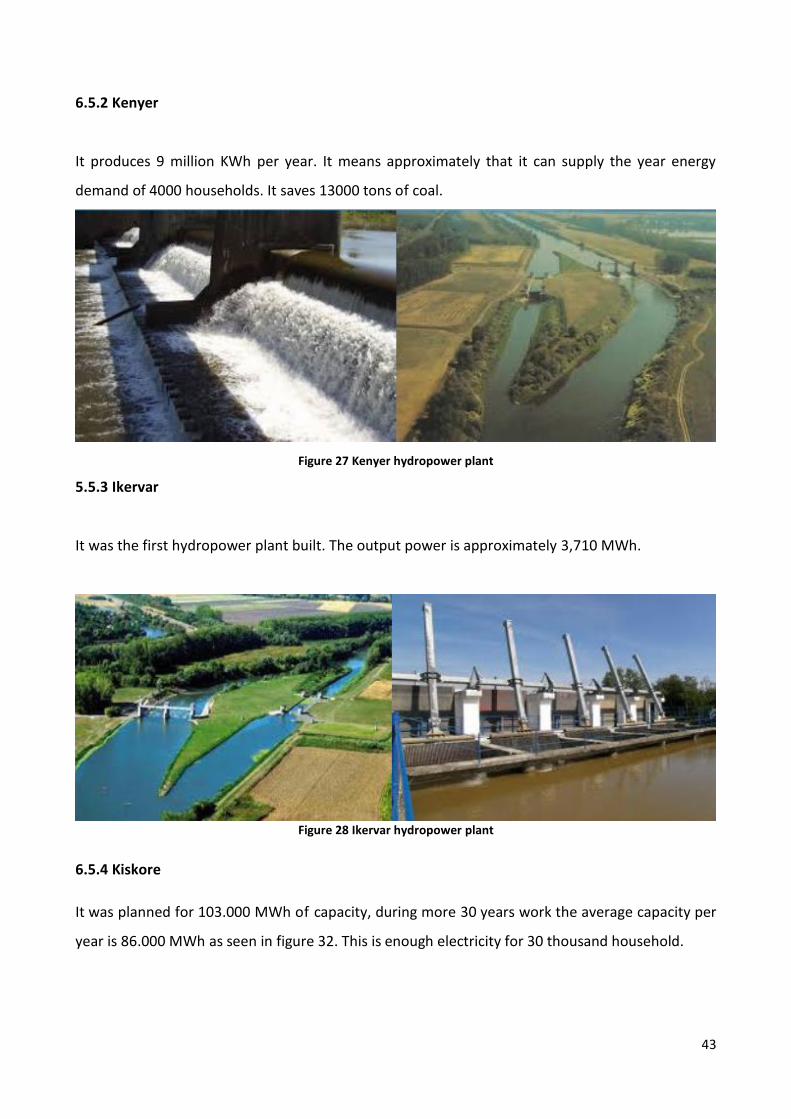
6.5.2 Kenyer
It produces 9 million KWh per year. It means approximately that it can supply the year energy
demand of 4000 households. It saves 13000 tons of coal.
Figure 27 Kenyer hydropower plant
5.5.3 Ikervar
It was the first hydropower plant built. The output power is approximately 3,710 MWh.
Figure 28 Ikervar hydropower plant
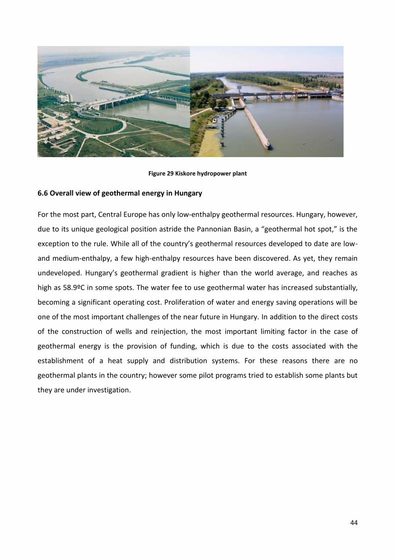
6.5.4 Kiskore
It was planned for 103.000 MWh of capacity, during more 30 years work the average capacity per
year is 86.000 MWh as seen in figure 32. This is enough electricity for 30 thousand household.
44
Figure 29 Kiskore hydropower plant
6.6 Overall view of geothermal energy in Hungary
For the most part, Central Europe has only low-enthalpy geothermal resources. Hungary, however,
due to its unique geological position astride the Pannonian Basin, a “geothermal hot spot,” is the
exception to the rule. While all of the country’s geothermal resources developed to date are low-
and medium-enthalpy, a few high-enthalpy resources have been discovered. As yet, they remain
undeveloped. Hungary’s geothermal gradient is higher than the world average, and reaches as
high as 58.9ºC in some spots. The water fee to use geothermal water has increased substantially,
becoming a significant operating cost. Proliferation of water and energy saving operations will be
one of the most important challenges of the near future in Hungary. In addition to the direct costs
of the construction of wells and reinjection, the most important limiting factor in the case of
geothermal energy is the provision of funding, which is due to the costs associated with the
establishment of a heat supply and distribution systems. For these reasons there are no
geothermal plants in the country; however some pilot programs tried to establish some plants but
they are under investigation.

45
Figure 30 Geothermal resource
Figure 31 Wellhead Temperature Regions of Water Wells areas
6.7 Overall view of photovoltaic energy in Hungary
Hungary has good potential for the use of solar energy. The number of sunny hours in Hungary is
between 1,950-2,150 per year at an intensity of 1.200 kWh/m2 per year. Unfortunately Hungarian
photovoltaic market is not well-developed. At the end of 2012 the photovoltaic plants in Hungary

46
have 6 MW cumulative installed capacity. The main reason behind the slow market expansion is
the low and non-functional feed-in tariff: there is a mandatory buy-back of the solar electricity,
but feed-in tariff is only approximately 0.11 €/kWh. In this way the time of payback is very long
and not guaranteed. Therefore in Hungary the tariff does not fit the standard of other countries
thus not making the growth of the market fast. There has been a plan to introduce a "classic" feed-
in tariff in Hungary for years, however in early 2013 it was again postponed, and it cannot be
expected before 2014.
According to Ernst & Young, Hungary has high solar irradiation, but the country struggles with its
insufficient grid capacity and very difficult permitting processes. In Hungary the number of solar
PV installation was increased in 2012, both by private and local authorities and the business field.
The average capacity is lower than 50 kWp. These investments do not require permit for the
installation.
Table 9 Installed and cumulated capacity in 2012 in Hungary
Applications Cumulated in 2011 (in
kWp)
Installed in 2012 (in
kWp)
Cumulated in 2012
(in kWp)
Off grid 400 100 500
On grid 2338 870 3238
Total 2738 970 3738
Big installations are rare. The first installations of PV systems have started at the beginning of
2000s. 2006 was the first year when the on-grid PV capacity exceeded the off-grid capacity and it
has predominated since then. In 2011 a 400 kWp installation began its operation in Újszilvás, at
present it has the biggest solar PV capacity in Hungary, but another project is under construction
in Szeged with 600 kWp. In 2011 the on-grid capacity was 1,900 and off-grid was 400 kW. In the
long run the rooftop and building integrated PV system applications are expected to be dominant.
6.7.1 PV history in Hungary
In 1973 the photovoltaic development started. At the end of 1975 there was the first installation.
In 1979 the silicon solar cell was developed and his efficiency achieved about 15%, which was
patented. In 1982 the PV Working Group was founded in the Hungarian Electro technical
47
Association. Later, in 1983 the Hungarian Solar Energy Society was founded and then, in 1989, the
Pannonglas SOLARLABS. These are the first companies to develop and build solar systems and
photovoltaic systems. Nowadays there are a lot of companies that are trying to improve and
achieve better and better results about efficiency.
PV applications in Hungary are essentially divisible in 4 categories:
Off grid systems (80 KWp)
Grid connected systems (55 KWp)
Quasi-autonomous power supplies (3 KWp)
Consumer products (n.a)
The PV installation instead has 3 big areas:
For buildings and for other objects
For free land areas
Data input: Hungarian statistical yearbook
Some potential data about PV in Hungary
1. Solar modules could be installed mainly on one side of the saddle roofs and on 0.431*flat
roofs.
2. Solar modules could be installed really only 50% of the principle areas and 25% of the
railway. (shading & others).
3. Because of orientation loss the effective solar areas are with 10% lower.
4. Calculating with 10% average module efficiency 1 m solar module nominal power = 100 Wp
5. Calculating with 80% matching and other conversion losses 1 kWp solar arrays produce
yearly average in Hungary at different tilt angles as follows: at 30° 1200 kWh/year, at 45°
1150 kWh/year and at 60° 1100 kWh/year.
The yearly average electrical energy production of the solar equipment to be installed potentially
in Hungary is 486 billion kWh. The yearly demand of electrical energy in Hungary today is less than
40 billion kWh. That means the potential is more than 12 fold. Increasing the number of PV fields
means more buildings facades but less solar thermal collectors.

48
Figure 32 First PV installation in Hungary 1975 (Off grid)
Figure 33 10 kWp grid connected PV systems
49
7 Cost analysis
Solar energy is a very important resource, it is free and unlimited because it is from the sun, but
the most important fact is that it is CLEAN. That is something priceless, because it does not harm
humans at all with CO2 or other dangerous substances. Obviously, there is a market which sets
prices for the supply, the demand and the value of the object. In the next paragraph we want to
analyze the trend of the selling and of the price of photovoltaic panels in the last few years.
7.1 Overview of global trend
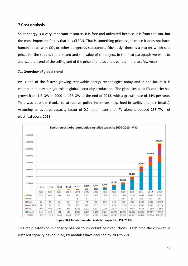
PV is one of the fastest growing renewable energy technologies today and in the future it is
estimated to play a major role in global electricity production. The global installed PV capacity has
grown from 1.8 GW in 2000 to 136 GW at the end of 2013, with a growth rate of 44% per year.
That was possible thanks to attractive policy incentives (e.g. feed-in tariffs and tax breaks).
Assuming an average capacity factor of 0.2 that means that PV alone produced 235 TWh of
electrical power2013
Figure 34 Global cumulated installed capacity (EPIA 2013)
This rapid extension in capacity has led to important cost reductions. Each time the cumulative
installed capacity has doubled, PV modules have declined by 20% to 22%.

50
Till mid-1990s, most PV systems were off-grid applications for telecommunications, remote houses
and rural electricity supply. Driven by various support and incentive schemes introduced by most
countries the number of grid-connected application increased quickly. In the last decade grid-
connected installations have overrun the off-grid applications, thus becoming the larger sector of
PV technologies. The growth in the utility-scale systems has also accelerated in recent years and
now has become a significant market.
In 2010, new installed PV capacity was 16.6 GW. Most of its growth was possible thanks to the
quick expansion of the German and Italian markets. With 7.4 GW installed in Germany in just one
year, the country continues to dominate the global PV market. Italy installed 2.3GW, starting to
take advantage of its wide solar resources.
In 2011, 27.7 GW of new PV capacity was installed, 66% more than in 2010. Europe accounted for
around 75% (20.9 GW) of all new capacity added in 2011. Italy, consolidated from its growth in
2010, added an impressive 9 GW of new capacity, increasing the total installed capacity by 260%.
Germany added 7.5 GW in 2011. Six countries added more than one GW in 2011 (i.e. Italy,
Germany, China, United States, Japan and France).
Facing the worldwide financial crisis started in 2009, 2012 is a problematic year for the PV market.
From the graphic below we can see how the market had a break in growth.
Figure 35 Global installed capacity (EPIA 2013)

51
The capacity installed in 2012 was a little bit less than 2011, thus marking the first negative trend
for the market. Moreover, if we focus on the European market, we see negative data emerging
from the graphic. In 2012 17 MW were installed in Europe instead of the 22 MW in 2011. This
means a contraction of 22% of the market. It was the year of the record for Germany with 11.4
GW, thus maintaining a reasonable level of installation in the European market. The other share
came from Italy. Aside from these two, the UK, Greece, Bulgaria and Belgium provided a large part
of the European market development.
Figure 36 Installed capacity in Europe
2013 marks a relevant reduction in the market, about 7 GW less than 2011 (41% less than the
previous year). The decline of Germany and Italy as the main protagonists of the European market
was confirmed. While the sum of the market in other countries remained around 6 MW, the two
countries provided just 5 MW, with a substantial reduction compared to the previous year. Also in
other countries of EU there was a decrease of the market, like Belgium and France, but that was
compensated by the boom in Greece and Romania. Anyway, despite the crisis, some
developments were achieved in the UK, and in some other smaller market countries, such as
Switzerland, the Netherlands and Austria.
Europe’s PV development was unreached for a long time till 2013. The USA and Japan, once PV
pioneers, used to be behind Europe in terms of PV penetration, whereas China has already
reached their level in just a few years of fast development.
52
The development of PV has usually corresponded to economic development; first starting in OECD
countries (Europe, North America, Japan, Australia), then spreading in emerging countries.
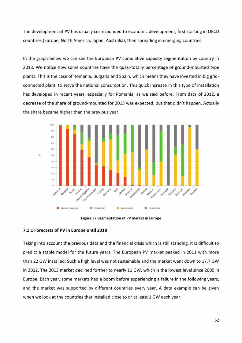
In the graph below we can see the European PV cumulative capacity segmentation by country in
2013. We notice how some countries have the quasi-totally percentage of ground-mounted type
plants. This is the case of Romania, Bulgaria and Spain, which means they have invested in big grid-
connected plant, to serve the national consumption. This quick increase in this type of installation
has developed in recent years, especially for Romania, as we said before. From data of 2012, a
decrease of the share of ground-mounted for 2013 was expected, but that didn’t happen. Actually
the share became higher than the previous year.
Figure 37 Segmentation of PV market in Europe
7.1.1 Forecasts of PV in Europe until 2018
Taking into account the previous data and the financial crisis which is still standing, it is difficult to
predict a stable model for the future years. The European PV market peaked in 2011 with more
than 22 GW installed. Such a high level was not sustainable and the market went down to 17.7 GW
in 2012. The 2013 market declined further to nearly 11 GW, which is the lowest level since 2009 in
Europe. Each year, some markets had a boom before experiencing a failure in the following years,
and the market was supported by different countries every year. A data example can be given
when we look at the countries that installed close to or at least 1 GW each year.

53
The instability of markets in Europe leads to say that there are no countries in Europe that once
experienced a serious PV boom can maintain the same market level, with the exception of
Germany.
Besides, the traumatic decrease of some FiT programs reduced some markets in 2014, with a
difficult possibility of emerging markets in Europe that could mitigate the decline.
In the High Scenario, the market could stabilize in 2014 and grow again from 2015 onwards, driven
by the approaching competitiveness of PV and emerging markets in Europe. To reach this level we
need a stabilization in the wide European market (Germany, Italy) and keeping on the current
policies in UK and growing again in Spain and France and in the other countries which entered the
market in the past few years.
Figure 38 Forecasts of the installed capacity in Europe
In this way the total capacity installed in Europe by 2018 could achieve between 118 and 156 GW
Figure 39 Forecasts of the cumulated installed capacity in Europe
54
In the coming years it will be worth focusing on the countries where PV has not developed yet,
because they have not taken advantage of their potential yet and also for the single chance to
improve and experience a different market development than what has been experienced until
now in most European countries. The history of PV shows that a stable policy structure using
support schemes in a balanced way gains market confidence. Poland, Croatia and Hungary can
develop in the coming years in different ways. Also outside the European Union, Turkey and some
Balkan states will become significant points. For markets developed in previous years, the
recovery of France should be carefully followed and animated in a way that fits the specifics of this
country. Also in Spain PV will not resume unless solutions are found to struggle the relative
isolation of the country from a grid perspective. Finally, the self-consumption shows a growth of
general interest, but in the real markets it remains unsure because the regulatory framework
conditions are unstable and not reliable, especially charges and taxes. In 2013, the sum of
installations that were driven by self-consumption in Europe amounted to over 2 GW. The hope of
PV development for Europe is the growth of the self-consumption like the main subject which has
to be as fast as possible.
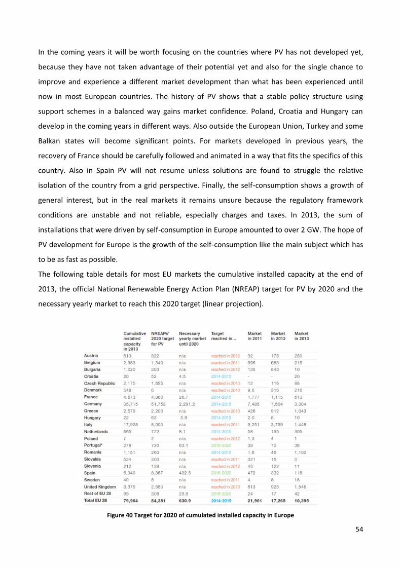
The following table details for most EU markets the cumulative installed capacity at the end of
2013, the official National Renewable Energy Action Plan (NREAP) target for PV by 2020 and the
necessary yearly market to reach this 2020 target (linear projection).
Figure 40 Target for 2020 of cumulated installed capacity in Europe

55
7.2 Price trend for PV systems
From the beginning of the first application in the far 1979 up to now, the price of PV modules has
decreased rapidly and constantly. Usually, the price is not expressed in Euro, but in Euro per Watt.
In the graph below we can see how the price trend in the last decades has dropped down fast.
Figure 41 Prices fall of modules from 1979
An observation similar to the famous Moore's Law can be made: it states that prices for solar cells
and panels fall by 22 per cent for every doubling of industry capacity. In the graph it is
unfortunately not clear due to the logarithmic scale.
As we can see the price in the far 1979 was US$ 20 for Wp for CdTe technology, in 2014 it is US$
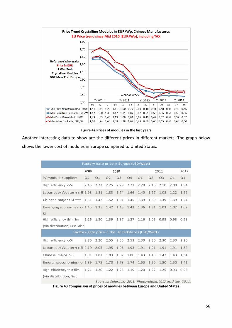
1.05. The reduction of the price is about 95%. If we focus in the last few years the picture that
emerges from Europe is shown below. The decrease in 4 years is more than 1 euro per watt, a 62%
drop. This data is related to the wide spread of the technology.
56
Figure 42 Prices of modules in the last years
Another interesting data to show are the different prices in different markets. The graph below
shows the lower cost of modules in Europe compared to United States.
Factory-gate price in Europe (USD/Watt)
2009 2010 2011 2012
PV module suppliers Q4 Q1 Q2 Q3 Q4 Q1 Q2 Q3 Q4 Q1
High efficiency c-Si 2.45 2.22 2.25 2.29 2.21 2.20 2.15 2.10 2.00 1.94
Japanese/Western c-Si
**
1.98 1.81 1.83 1.74 1.66 1.40 1.27 1.08 1.22 1.22
Chinese major c-Si *** 1.51 1.42 1.52 1.51 1.45 1.39 1.39 1.39 1.39 1.24
Emerging economies c-
Si
****
1.45 1.35 1.42 1.43 1.43 1.36 1.31 1.03 1.02 1.02
High efficiency thin-film
(via distribution, First Solar
)
1.26 1.30 1.39 1.37 1.27 1.16 1.05 0.98 0.93 0.93
Factory-gate price in the United States (USD/Watt)
High efficiency c-Si 2.86 2.20 2.55 2.55 2.53 2.30 2.30 2.30 2.30 2.20
Japanese/Western c-Si 2.10 2.05 1.95 1.95 1.93 1.91 1.91 1.91 1.91 1.82
Chinese major c-Si 1.91 1.87 1.83 1.87 1.80 1.43 1.43 1.47 1.43 1.34
Emerging economies- c-
Si
1.89 1.75 1.70 1.78 1.74 1.50 1.50 1.50 1.50 1.41
High efficiency thin-film
(via distribution, First
Solar)
1.21 1.20 1.22 1.25 1.19 1.20 1.22 1.25 0.93 0.93
Sources: Solarbuzz, 2011; Photovoltaik, 2012 and Luo, 2011.
Figure 43 Comparison of prices of modules between Europe and United States

57
The reason of this small increment of price in the United States is due to the mature market in
Europe developed some years earlier and the constant research and investments which allow
Europe to gain the supremacy in the production and application.
The price of the module is usually shared in this way:
Figure 44 Shared price of module
However, the price of a PV system is not just the module, but there also some other costs named
BOS (Balance of system costs), which usually include the inverter, the business process, the
structural installation, the racking, site preparation attachments, electrical installation, wiring and
transformers. For utility-scale PV plants, it can be as low as 20% (for a simple grid-connected
system) or as high as 70% (for an off-grid system), with 40% being representative of a standard
utility-scale ground mounted system. The average cost of BOS and installation for PV systems is in
the range of USD 1.6 to USD 1.85/W in 2010.
Rooftop-mounted systems have BOS costs about USD 0.25/W higher than ground-mounted
systems, primarily due to the additional cost of preparing the roof to receive the PV modules and
slightly more costly installation (EPIA 2010, Photon 2011).
The inverter is one of the most important components of a PV system. It converts DC electricity
from the PV modules into AC electricity to feed the grid. The size of inverters ranges from a small
textbook devices for residential mount to large container solutions for utility-scale systems, like PV
plants. The size and numbers of inverters required depend on the installed PV capacity. Inverters

58
are the primary power electronics components of a PV system and typically they share the 5% of
the total installed system costs. In 2012 the inverter costs ranged from 0.15 €/W to 0.35 €/W.
Larger systems record lower inverter costs per unit of capacity.
Figure 45 Inverters efficiency, cost and reliability
Mounting structures and racking hardware components for PV modules are usually already
designed systems of aluminium or steel tracks. They share more and less the 6% of the total
capital cost of PV costs.
Mounting structures are different due to the location of the site. If they are for rooftop for
residential and commercial use they have some type of solutions, for ground-mounted the set is
different.
Combiner box and miscellaneous electrical components incorporate all remaining installation
components, including combiner boxes, wires/conductors, conduits, data monitoring systems, and
other miscellaneous hardware.
Site preparation and system installation are the largest components of the BOS and installation
costs. They include site preparation, any physical construction works, installation and connection
of the system. Costs of labour, usually the biggest quota, increase rapidly the installation costs,
and vary by project and country.
System design, management and administrative costs incorporate system design and
management costs for project, funding and permissions. For residential and small scale PV
systems, these costs are often included in the total PV installed prices decided by companies. For

59
large scale installations these costs can be handled directly by the sponsor or given to a service
provider. In the United States in 2010 they accounted for an average 37% of the total system costs
(GTM Research, 2011).
Electricity storage systems for off-grid PV systems capable of provide electricity at night or during
cloudy periods. A lot of electricity storage systems are on the market, or under development, but
they are expensive and seem to be more suitable for large-scale applications. Standard lead-acid
batteries have been the best technology until now for small scale systems. Battery raises the cost
of the PV system, but much less than grid connection in remote areas. Their use is necessary not
only for remote residential and commercial applications, but also for off-grid repeater stations for
mobile phones, radio beacons, etc. The lifetime of a battery, assuming the discharge does not
reach the 20% of the capacity, is approximately 10 years. Another negative aspect to mention is
the capacity. If for example we have a PV system which can generate 1 KWp, usually the capacity
of the battery shall be around 5 times the power of the system, thus 5 KWp. The cost is near to
1500 €/KW for generated energy, without considering a battery change controller.
The graphic below shows a sum of the total cost of a whole PV system.
Figure 46 Shared price of a PV plant
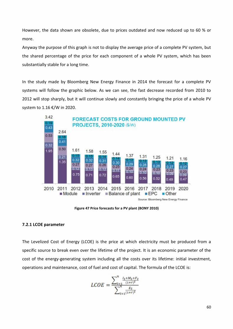
60
However, the data shown are obsolete, due to prices outdated and now reduced up to 60 % or
more.
Anyway the purpose of this graph is not to display the average price of a complete PV system, but
the shared percentage of the price for each component of a whole PV system, which has been
substantially stable for a long time.
In the study made by Bloomberg New Energy Finance in 2014 the forecast for a complete PV
systems will follow the graphic below. As we can see, the fast decrease recorded from 2010 to
2012 will stop sharply, but it will continue slowly and constantly bringing the price of a whole PV
system to 1.16 €/W in 2020.
Figure 47 Price forecasts for a PV plant (BONY 2010)
7.2.1 LCOE parameter
The Levelized Cost of Energy (LCOE) is the price at which electricity must be produced from a
specific source to break even over the lifetime of the project. It is an economic parameter of the
cost of the energy-generating system including all the costs over its lifetime: initial investment,
operations and maintenance, cost of fuel and cost of capital. The formula of the LCOE is:
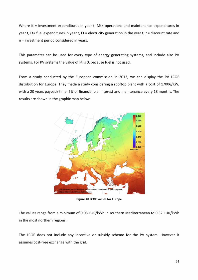
61
Where It = Investment expenditures in year t, Mt= operations and maintenance expenditures in
year t, Ft= fuel expenditures in year t, Et = electricity generation in the year t, r = discount rate and
n = investment period considered in years.
This parameter can be used for every type of energy generating systems, and include also PV
systems. For PV systems the value of Ft is 0, because fuel is not used.
From a study conducted by the European commission in 2013, we can display the PV LCOE
distribution for Europe. They made a study considering a rooftop plant with a cost of 1700€/KW,
with a 20 years payback time, 5% of financial p.a. interest and maintenance every 18 months. The
results are shown in the graphic map below.
Figure 48 LCOE values for Europe
The values range from a minimum of 0.08 EUR/kWh in southern Mediterranean to 0.32 EUR/kWh
in the most northern regions.
The LCOE does not include any incentive or subsidy scheme for the PV system. However it
assumes cost-free exchange with the grid.
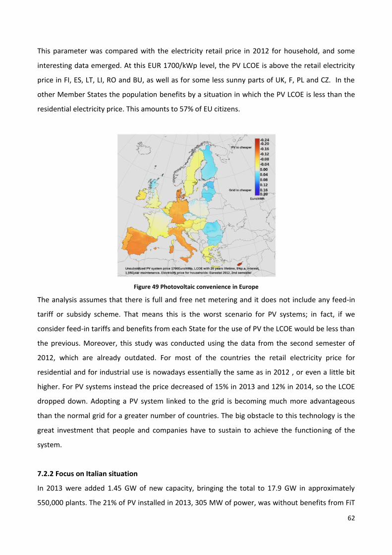
62
This parameter was compared with the electricity retail price in 2012 for household, and some
interesting data emerged. At this EUR 1700/kWp level, the PV LCOE is above the retail electricity
price in FI, ES, LT, LI, RO and BU, as well as for some less sunny parts of UK, F, PL and CZ. In the
other Member States the population benefits by a situation in which the PV LCOE is less than the
residential electricity price. This amounts to 57% of EU citizens.
Figure 49 Photovoltaic convenience in Europe
The analysis assumes that there is full and free net metering and it does not include any feed-in
tariff or subsidy scheme. That means this is the worst scenario for PV systems; in fact, if we
consider feed-in tariffs and benefits from each State for the use of PV the LCOE would be less than
the previous. Moreover, this study was conducted using the data from the second semester of
2012, which are already outdated. For most of the countries the retail electricity price for
residential and for industrial use is nowadays essentially the same as in 2012 , or even a little bit
higher. For PV systems instead the price decreased of 15% in 2013 and 12% in 2014, so the LCOE
dropped down. Adopting a PV system linked to the grid is becoming much more advantageous
than the normal grid for a greater number of countries. The big obstacle to this technology is the
great investment that people and companies have to sustain to achieve the functioning of the
system.
7.2.2 Focus on Italian situation
In 2013 were added 1.45 GW of new capacity, bringing the total to 17.9 GW in approximately
550,000 plants. The 21% of PV installed in 2013, 305 MW of power, was without benefits from FiT
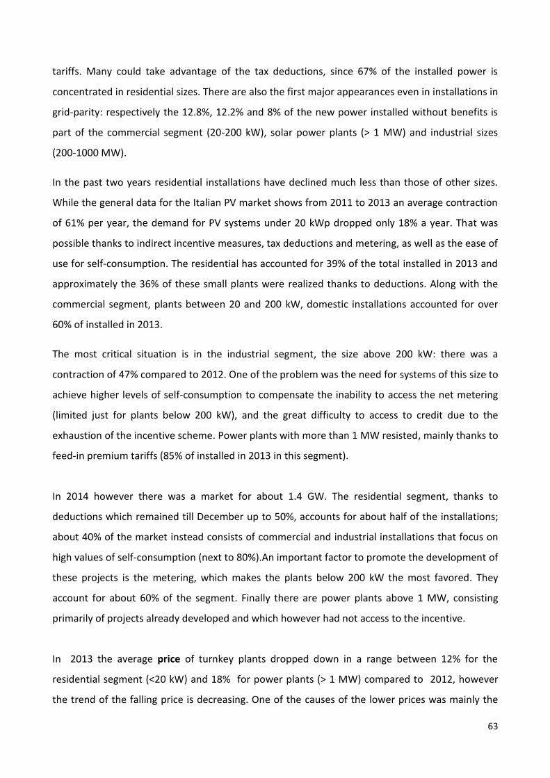
63
tariffs. Many could take advantage of the tax deductions, since 67% of the installed power is
concentrated in residential sizes. There are also the first major appearances even in installations in
grid-parity: respectively the 12.8%, 12.2% and 8% of the new power installed without benefits is
part of the commercial segment (20-200 kW), solar power plants (> 1 MW) and industrial sizes
(200-1000 MW).
In the past two years residential installations have declined much less than those of other sizes.
While the general data for the Italian PV market shows from 2011 to 2013 an average contraction
of 61% per year, the demand for PV systems under 20 kWp dropped only 18% a year. That was
possible thanks to indirect incentive measures, tax deductions and metering, as well as the ease of
use for self-consumption. The residential has accounted for 39% of the total installed in 2013 and
approximately the 36% of these small plants were realized thanks to deductions. Along with the
commercial segment, plants between 20 and 200 kW, domestic installations accounted for over
60% of installed in 2013.
The most critical situation is in the industrial segment, the size above 200 kW: there was a
contraction of 47% compared to 2012. One of the problem was the need for systems of this size to
achieve higher levels of self-consumption to compensate the inability to access the net metering
(limited just for plants below 200 kW), and the great difficulty to access to credit due to the
exhaustion of the incentive scheme. Power plants with more than 1 MW resisted, mainly thanks to
feed-in premium tariffs (85% of installed in 2013 in this segment).
In 2014 however there was a market for about 1.4 GW. The residential segment, thanks to
deductions which remained till December up to 50%, accounts for about half of the installations;
about 40% of the market instead consists of commercial and industrial installations that focus on
high values of self-consumption (next to 80%).An important factor to promote the development of
these projects is the metering, which makes the plants below 200 kW the most favored. They
account for about 60% of the segment. Finally there are power plants above 1 MW, consisting
primarily of projects already developed and which however had not access to the incentive.
In 2013 the average price of turnkey plants dropped down in a range between 12% for the
residential segment (<20 kW) and 18% for power plants (> 1 MW) compared to 2012, however
the trend of the falling price is decreasing. One of the causes of the lower prices was mainly the

64
effect of oversupply, linked to modules and other components accumulated in the warehouses of
the distribution chain and sold with discount. Besides there was a reduction of the cost of the
components like inverter and design and installation, which followed the trend already shown in
2012.
For the new PV modules placed on the market during 2013, there was instead a substantial
stability. The fall of prices was arrested for the direct effect of the anti-dumping measures adopted
in all the European Union since March 2013 and confirmed in December 2013. Another reason is
the contraction of the European market (-42% approximately, from 17.5 GW in 2012 to 10.2 GW in
2013), which decreased the import of products from Asia, as they cost less than European PV
manufactures.
Focusing more specifically, the market however displayed a different trend for the different
technologies: an increase in the average price (between 8 and 9%) for the silicon mono and poly-
crystalline technology; the price of CdTe modules was substantially stable; a decrease of 7% for
amorphous silicon technology. Products from Europe, the US and Japan have shown a reduction in
the average price between 12 and 15%, far from previous years (-26% on 2012 and -38% in 2011).
The price of mono and poly-crystal silicon made in China even increased about 10%, for the effects
of anti-dumping.
Anyway the slowed collapse of prices has not brought great relief to Italian producers of modules:
the average levels of profits are still negative, due to the difficulties to reduce more production
costs. In particular, regarding silicon modules it is difficult to reach again sustainable values of
profit, or at least comparable to the values of 2010. For CdTe and a-SI (amorphous) modules the
state results a little bit better as the cost of production dropped down due to higher conversion
efficiency of the modules (in some cases more than 12%). That was possible by the results
obtained from researches made in 2012.
Important reductions have been recorded on prices in storage electrochemical technologies,
especially in reference to lead-acid batteries, which are the best solution for residential and small
commercial (<20 kWp) applications and presenting a storage capacity between 2.5 and 15 kWh.

65
With today’s prices, and tax deductions up to 50%, a plant produces energy at a cost of about 0.06
€/kWh, and without tax deductions at about 0.11 €/kWh. This is the actual real value of the energy
produced by the PV.
The trend expected till 2020 for the price of modules forecasts a reduction for each year between
-2% (in the first years) and -8% (from 2016). This reduction is much more restrained than the -26%
in 2012 and -40% in 2011. A reasonable forecast for 2020 seems to assume values below the 0.50
€/Wp in the case of silicon modules and near 0.40 €/Wp for the thin film according to the Energy
& Strategy Group.
These price forecasts are based on three main factors. The first is the way out of the state of
oversupply for the upstream stages of the production chain, also due to the phenomenon of
industry consolidation; the second is the lower incidence of the modules on the European market
from China, caused by compensation measures for anti-dumping and less use of aggressive pricing
policies by Asian operators on international markets due to result of their internal market growth.
The third factor is the increase in global demand.
In Italy there was a big boost for PV systems in the past years. That led to a FiT (feed-in tariff). A
feed-in tariff is a policy mechanism designed to accelerate investment in renewable energy
technologies, which is achieved by offering long-term contracts to renewable energy producers,
typically based on the cost of generation of each technology, which for PV are the highest. They
pay an equal amount for energy and moreover, if they require energy, they have access with a
discount price, named self-consumption.
For a long time Italy had one of the best FiT in Europe according to CONTO ENERGIA, due to the
unlimited resource of sunlight. Below are shown the feed-in tariffs and self-consumption tariffs for
most typical PV technologies.
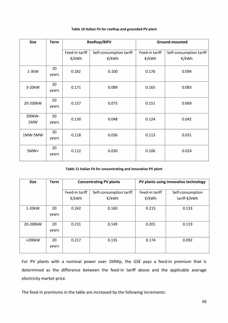
66
Table 10 Italian Fit for rooftop and grounded PV plant
Size Term Rooftop/BIPV Ground-mounted
Feed-in tariff
€/kWh
Self-consumption tariff
€/kWh
Feed-in tariff
€/kWh
Self-consumption tariff
€/kWh
1-3kW 20
years 0.182 0.100 0.176 0.094
3-20kW 20
years 0.171 0.089 0.165 0.083
20-200kW 20
years 0.157 0.075 0.151 0.069
200kW-
1MW
20
years 0.130 0.048 0.124 0.042
1MW-5MW 20
years 0.118 0.036 0.113 0.031
5MW+ 20
years 0.112 0.030 0.106 0.024
Table 11 Italian Fit for concentrating and innovative PV plant
Size Term Concentrating PV plants PV plants using innovative technology
Feed-in tariff
€/kWh
Self-consumption tariff
€/kWh
Feed-in tariff
€/kWh
Self-consumption
tariff €/kWh
1-20kW 20
years
0.242 0.160 0.215 0.133
20-200kW 20
years
0.231 0.149 0.201 0.119
>200kW 20
years
0.217 0.135 0.174 0.092
For PV plants with a nominal power over 1MWp, the GSE pays a feed-in premium that is
determined as the difference between the feed-in tariff above and the applicable average
electricity market price.
The feed-in premiums in the table are increased by the following increments:
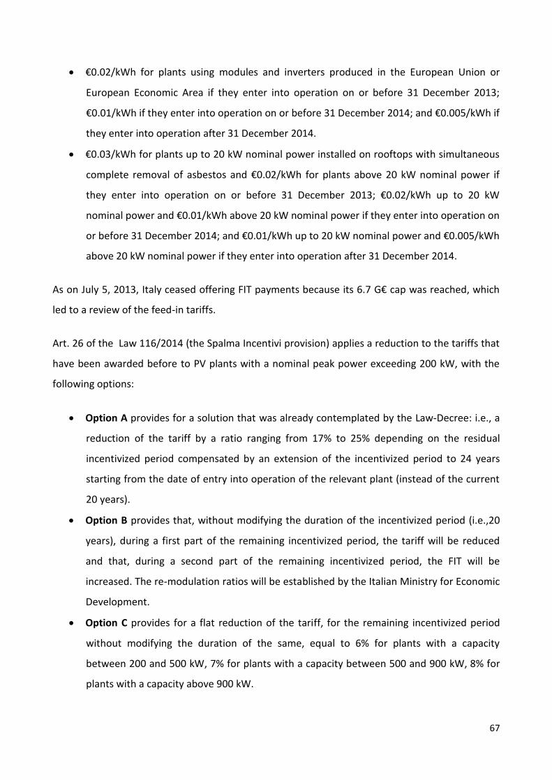
67
€0.02/kWh for plants using modules and inverters produced in the European Union or
European Economic Area if they enter into operation on or before 31 December 2013;
€0.01/kWh if they enter into operation on or before 31 December 2014; and €0.005/kWh if
they enter into operation after 31 December 2014.
€0.03/kWh for plants up to 20 kW nominal power installed on rooftops with simultaneous
complete removal of asbestos and €0.02/kWh for plants above 20 kW nominal power if
they enter into operation on or before 31 December 2013; €0.02/kWh up to 20 kW
nominal power and €0.01/kWh above 20 kW nominal power if they enter into operation on
or before 31 December 2014; and €0.01/kWh up to 20 kW nominal power and €0.005/kWh
above 20 kW nominal power if they enter into operation after 31 December 2014.
As on July 5, 2013, Italy ceased offering FIT payments because its 6.7 G€ cap was reached, which
led to a review of the feed-in tariffs.
Art. 26 of the Law 116/2014 (the Spalma Incentivi provision) applies a reduction to the tariffs that
have been awarded before to PV plants with a nominal peak power exceeding 200 kW, with the
following options:
Option A provides for a solution that was already contemplated by the Law-Decree: i.e., a
reduction of the tariff by a ratio ranging from 17% to 25% depending on the residual
incentivized period compensated by an extension of the incentivized period to 24 years
starting from the date of entry into operation of the relevant plant (instead of the current
20 years).
Option B provides that, without modifying the duration of the incentivized period (i.e.,20
years), during a first part of the remaining incentivized period, the tariff will be reduced
and that, during a second part of the remaining incentivized period, the FIT will be
increased. The re-modulation ratios will be established by the Italian Ministry for Economic
Development.
Option C provides for a flat reduction of the tariff, for the remaining incentivized period
without modifying the duration of the same, equal to 6% for plants with a capacity
between 200 and 500 kW, 7% for plants with a capacity between 500 and 900 kW, 8% for
plants with a capacity above 900 kW.
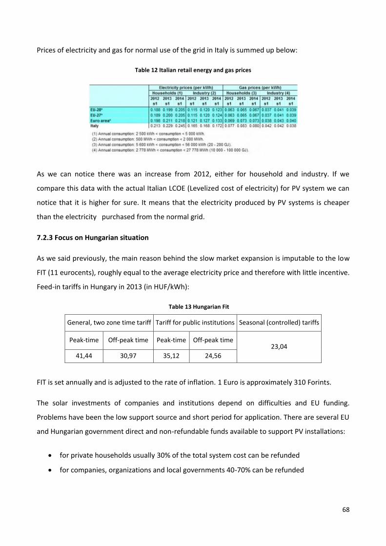
68
Prices of electricity and gas for normal use of the grid in Italy is summed up below:
Table 12 Italian retail energy and gas prices
As we can notice there was an increase from 2012, either for household and industry. If we
compare this data with the actual Italian LCOE (Levelized cost of electricity) for PV system we can
notice that it is higher for sure. It means that the electricity produced by PV systems is cheaper
than the electricity purchased from the normal grid.
7.2.3 Focus on Hungarian situation
As we said previously, the main reason behind the slow market expansion is imputable to the low
FIT (11 eurocents), roughly equal to the average electricity price and therefore with little incentive.
Feed-in tariffs in Hungary in 2013 (in HUF/kWh):
Table 13 Hungarian Fit
General, two zone time tariff Tariff for public institutions Seasonal (controlled) tariffs
Peak-time Off-peak time Peak-time Off-peak time 23,04
41,44 30,97 35,12 24,56
FIT is set annually and is adjusted to the rate of inflation. 1 Euro is approximately 310 Forints.
The solar investments of companies and institutions depend on difficulties and EU funding.
Problems have been the low support source and short period for application. There are several EU
and Hungarian government direct and non-refundable funds available to support PV installations:
for private households usually 30% of the total system cost can be refunded
for companies, organizations and local governments 40-70% can be refunded
69
The access to the grid for solar systems in Hungary is guaranteed by law, but systems of capacity
higher than 500 kWp need to obtain a permit from the Hungarian Energy Office. Small installations
are subject to utility operator permit. There are six utility operators in Hungary, the most
important is ELMÜ. It is a pathfinder, introducing simplified procedure for PV grid connection.
Most of the on-grid PV systems are located in the central region which ELMÜ is also situated.
Other utilities try to harmonize their procedures with this operator.
The electricity introduced through the grid must not exceed 2/3 of the electricity consumed. If it is
not the case, then such installation would be considered like a small electric power station and
stricter grid connecting technical requirements would apply, which means less profits and more
money to pay. The Hungarian Certificate of the inverters is one of the main problems with PV
plants. It is a big obstacle in grid connecting process in Hungary, and hits every size of systems.
This certificate is required by utilities operators before opening the access to their grid.
Certificates are issued by the Hungarian Testing Laboratory. This requirement results in extra costs
for investors. Furthermore the lack of capital and effective governmental support cut the chance
to build physical installations. Experiences have shown that without governmental granting
support the sector development simply is on halt.
Moreover the levy of HUF 114/kg (0.36 €/kg) was introduced to cover the cost of disposing the
panels when they reach the end of their life according to an official rule from the agriculture
ministry quoted in local media reports.
Despite this unlikely situation, there has been a growing interest in solar PV from municipalities,
not only in investments, development and design but on eco fields too. Almost 170 applications
were ordered to the Solar Corona Championship in 2012 from local governments. The winner had
the highest proportion of solar PV or collector. One of the winner was Nagypáli, second was
Újszilvás with the biggest solar PV system, and the third was Csitár-Nógrádgárdony.
The recent rise in the demand for solar PV is due to the increase electricity bills becoming too
expensive for Hungarians, while the progress is partly supported by growing environmental
concerns.

70
Table 14 Hungarian retail electricity and gas prices
From the studies previously reported it emerges that the LCOE is still less than the price of retail
electricity. The difference is not remarkable as for Italy, but it is anyway a positive data. That
means, as well as for Italy, a PV system appears cheaper than purchasing the energy from the grid.
The PV market in Hungary is growing, slowly but stable. Some forecast were made by Solar
Experts, in which they expected around 500 MW of capacity. Below is displayed the trend.
Figure 50 Forecasts for cumulated installed capacity in Hungary

71
8 Montalto di Castro Photovoltaic Power Station
The biggest large-scale PV plant in Europe is in Italy in Montalto di Castro. The total output is 85
MWp. This is enough to supply a city with a population of about 24,000 with electrical energy
around-the-clock using solely the power of the sun. In the case of the PV power station in
Montalto di Castro this saves 78,000 tonnes of CO2 emissions every year.
The photovoltaic park of Montalto di Castro is in the region of Lazio, near Viterbo. The project was
designed by the Sunray Company, and then bought by the SunPower Company.
The project was developed through several phases. In the first phase the capacity of the plant was
about 24 MW, and it was completed at the end of 2009.
The second one was commissioned in 2010 (8 MW), the third and the fourth were finished at the
end of 2010, for an amount of 44 MW.
At the beginning of 2011 the company SunPower sold the whole park to an association of
international investors. As SunPower designed and built the solar photovoltaic park it will continue
to provide assistance and maintenance.
Perfectly integrated into the landscape, the solar farm is not a problem for the population that
considered the energy, generated from modules of the photovoltaic park, an opportunity for
development and growth. The plant provides clean energy and reduction of pollutants in the
atmosphere.
Figure 51 View of the Montalto di Castro Power Plants

72
8.1 Principal data
The main data of the PV power plant are:
Inverters: 124 x SC 630HE
Developer: SunPowerCorp
SunPower Product: SunPower E18 / 305W panels , SunPower T0 tracker
Site area: 166 acres (1.7 km2)
Units operational: 276,156
Nameplate capacity: 84.23 MW (DC)
Capacity factor: 19%
Annual generation: 140 GW
8.2 Costs of the plant
First and second phase: 255 millions of euros (51 MW)
Third and fourth phase: 195,2 millions of euros (to achieve 84 MW)
Sun power E18: 400 Euros
Sc 630HE: 150000 Euros
SunPower T0 tracker: 4 Euros/Watt
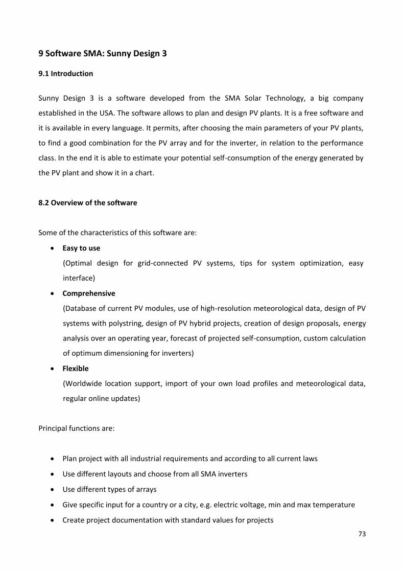
73
9 Software SMA: Sunny Design 3
9.1 Introduction
Sunny Design 3 is a software developed from the SMA Solar Technology, a big company
established in the USA. The software allows to plan and design PV plants. It is a free software and
it is available in every language. It permits, after choosing the main parameters of your PV plants,
to find a good combination for the PV array and for the inverter, in relation to the performance
class. In the end it is able to estimate your potential self-consumption of the energy generated by
the PV plant and show it in a chart.
8.2 Overview of the software
Some of the characteristics of this software are:
Easy to use
(Optimal design for grid-connected PV systems, tips for system optimization, easy
interface)
Comprehensive
(Database of current PV modules, use of high-resolution meteorological data, design of PV
systems with polystring, design of PV hybrid projects, creation of design proposals, energy
analysis over an operating year, forecast of projected self-consumption, custom calculation
of optimum dimensioning for inverters)
Flexible
(Worldwide location support, import of your own load profiles and meteorological data,
regular online updates)
Principal functions are:
Plan project with all industrial requirements and according to all current laws
Use different layouts and choose from all SMA inverters
Use different types of arrays
Give specific input for a country or a city, e.g. electric voltage, min and max temperature
Create project documentation with standard values for projects

74
Detect potential self-consumption of PV energy
Create an own site with accurate meteorological data
Create own PV modules
Automatically check operation data of the planned PV plant
Cable dimensioning
The software is mainly divided into 7 sections:
1. First section
In the first section we can choose main data of project. We can choose the name,
costumers, the location and type of electric voltage. After choosing the location the
program loads automatically common data for that position, like temperatures and electric
voltage for that state, example Budapest (min -22°, max 34°, voltage 230V). It is also
possible to modify meteorological data. The parameters are 3: annual extreme low and
high temperature, average high temperature. Changing these parameters make some
effects:
decreasing the minimum temperature causes an increasing of the maximum
voltage value of the PV modules
increasing the parameter called “annual extreme high temperature” causes a
decrease of the minimum voltage value of the power plant

75
Figure 52 First secton of Sunny Design 3
2. Second section
In this section we can define our load profile here and optionally add specific loads. We can
decide from household to industrial company or our own profile. The software
automatically loads the annual energy consumption from its database, but we can change
according our request. Then we can also specify number of person, hot water consumption
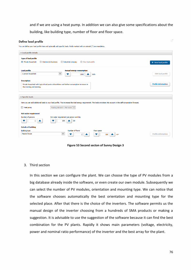
76
and if we are using a heat pump. In addition we can also give some specifications about the
building, like building type, number of floor and floor space.
Figure 53 Second secton of Sunny Design 3
3. Third section
In this section we can configure the plant. We can choose the type of PV modules from a
big database already inside the software, or even create our own module. Subsequently we
can select the number of PV modules, orientation and mounting type. We can notice that
the software chooses automatically the best orientation and mounting type for the
selected place. After that there is the choice of the inverters. The software permits us the
manual design of the inverter choosing from a hundreds of SMA products or making a
suggestion. It is advisable to use the suggestion of the software because it can find the best
combination for the PV plants. Rapidly it shows main parameters (voltage, electricity,
power and nominal ratio performance) of the inverter and the best array for the plant.

77
Figure 54 Third secton of Sunny Design 3
4. Fourth section
In this section the software automatically shows the best option for wire material, length
and the section. It also allows the selection of these parameters. After that it calculates the
power losses of the selected line.
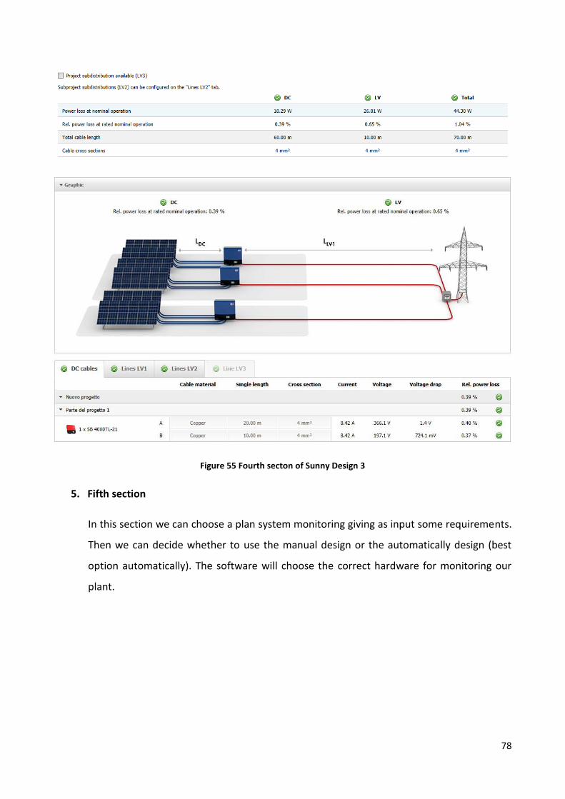
78
Figure 55 Fourth secton of Sunny Design 3
5. Fifth section
In this section we can choose a plan system monitoring giving as input some requirements.
Then we can decide whether to use the manual design or the automatically design (best
option automatically). The software will choose the correct hardware for monitoring our
plant.

79
Figure 56 Fifth secton of Sunny Design 3
6. Sixth section
Here we can determine our possible self-consumption of the produced PV energy. We can
choose if we want to use a battery to storage the temporary surplus of solar power, and
also we can generate graphic and data for the use of a heat pump.

80
Figure 57 Sixth secton of Sunny Design 3
7. Seventh section
In this section we can edit details on the cost structure and consider an analysis of the
economic viability of the PV project.
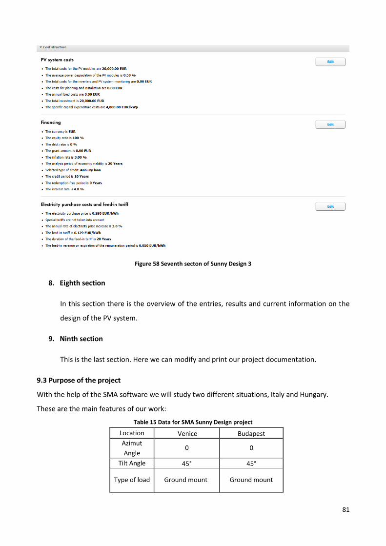
81
Figure 58 Seventh secton of Sunny Design 3
8. Eighth section
In this section there is the overview of the entries, results and current information on the
design of the PV system.
9. Ninth section
This is the last section. Here we can modify and print our project documentation.
9.3 Purpose of the project
With the help of the SMA software we will study two different situations, Italy and Hungary.
These are the main features of our work:
Table 15 Data for SMA Sunny Design project
Location Venice Budapest
Azimut
Angle 0 0
Tilt Angle 45° 45°
Type of load Ground mount Ground mount

82
Other important data to mention for our study is the annual total of global radiation. For Venice it
results 1326.29 kWh/m²a, instead for Budapest 1203.99 kWh/m²a. Already from this little
difference we can expect more production of energy in Italy then in Hungary.
The grid voltage was set for 230V, which is the normal setting for Italy and Hungary. The
photovoltaic peak power was chosen for 84.23 MW, which is the same power of the Montalto di
Castro Photovoltaic Power Station.
For each region 4 different types of photovoltaic panels were chosen. Then with the software we
tried to find the best solution with inverters maximizing the energy yield.
Types of photovoltaic panels are:
SMA Demo Poly 240
Schott Solar PV Inc Perform Mono 250 (UL)
Sharp ND-R250A5
Suntech Power STP300-VRM-1
Companies that produce these panels are the most famous around the world and they supply
more than the 90% of PV. First the software shows us the quantity of modules and inverters.
Table 16 Data for alternatives in SMA Sunny Design
pv modules # of pv modules inverters # of inverters
alternative 1 venice
SMA Demo Poly 240 350958 STP25000TL-30 + 3375
budapest MLX 60 + 1394
alternative 2
venice Schott Solar PV Inc
Perform Mono 250
(UL)
336920 STP25000TL-30
3438
budapest 3438
alternative 3 venice
Sharp ND-R250A5 336920 STP25000TL-30 3336
budapest MLX 60 + 1460
alternative 4 venice Suntech Power
STP300-VRM-1 280767
STP25000TL-30 3424
budapest MLX 60 + 1202
We can notice how for different types of pv modules correspond different types of inverters. That
is because every type of module has different characteristics, so to achieve the best solution we
need to use different type of inverters. We can also notice that for the same module we need to
use different types of inverters depending on the region we choose. The purpose of our plant is
not supplying the energy consumption for a household, but it is supplying the electric web. So
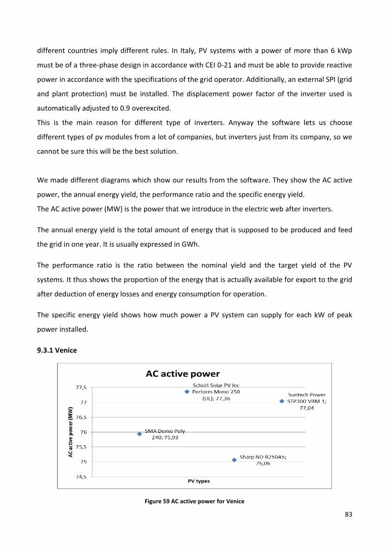
83
different countries imply different rules. In Italy, PV systems with a power of more than 6 kWp
must be of a three-phase design in accordance with CEI 0-21 and must be able to provide reactive
power in accordance with the specifications of the grid operator. Additionally, an external SPI (grid
and plant protection) must be installed. The displacement power factor of the inverter used is
automatically adjusted to 0.9 overexcited.
This is the main reason for different type of inverters. Anyway the software lets us choose
different types of pv modules from a lot of companies, but inverters just from its company, so we
cannot be sure this will be the best solution.
We made different diagrams which show our results from the software. They show the AC active
power, the annual energy yield, the performance ratio and the specific energy yield.
The AC active power (MW) is the power that we introduce in the electric web after inverters.
The annual energy yield is the total amount of energy that is supposed to be produced and feed
the grid in one year. It is usually expressed in GWh.
The performance ratio is the ratio between the nominal yield and the target yield of the PV
systems. It thus shows the proportion of the energy that is actually available for export to the grid
after deduction of energy losses and energy consumption for operation.
The specific energy yield shows how much power a PV system can supply for each kW of peak
power installed.
9.3.1 Venice
Figure 59 AC active power for Venice
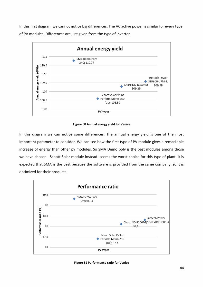
84
In this first diagram we cannot notice big differences. The AC active power is similar for every type
of PV modules. Differences are just given from the type of inverter.
Figure 60 Annual energy yield for Venice
In this diagram we can notice some differences. The annual energy yield is one of the most
important parameter to consider. We can see how the first type of PV module gives a remarkable
increase of energy than other pv modules. So SMA Demo poly is the best modules among those
we have chosen. Schott Solar module instead seems the worst choice for this type of plant. It is
expected that SMA is the best because the software is provided from the same company, so it is
optimized for their products.
Figure 61 Performance ratio for Venice

85
Also in this diagram we can notice that the best performance is from SMA Demo Poly, with an
amount of 89,3% , which is a good amount. Schott Solar is still the worst.
Figure 62 Specific energy yield for Venice
Also here we can see that the SMA Demo Poly is the best. The reasons are the same as before.
9.3.2 Budapest
Underneath there are results for Hungary-Budapest:
Figure 63 AC active power for Budapest
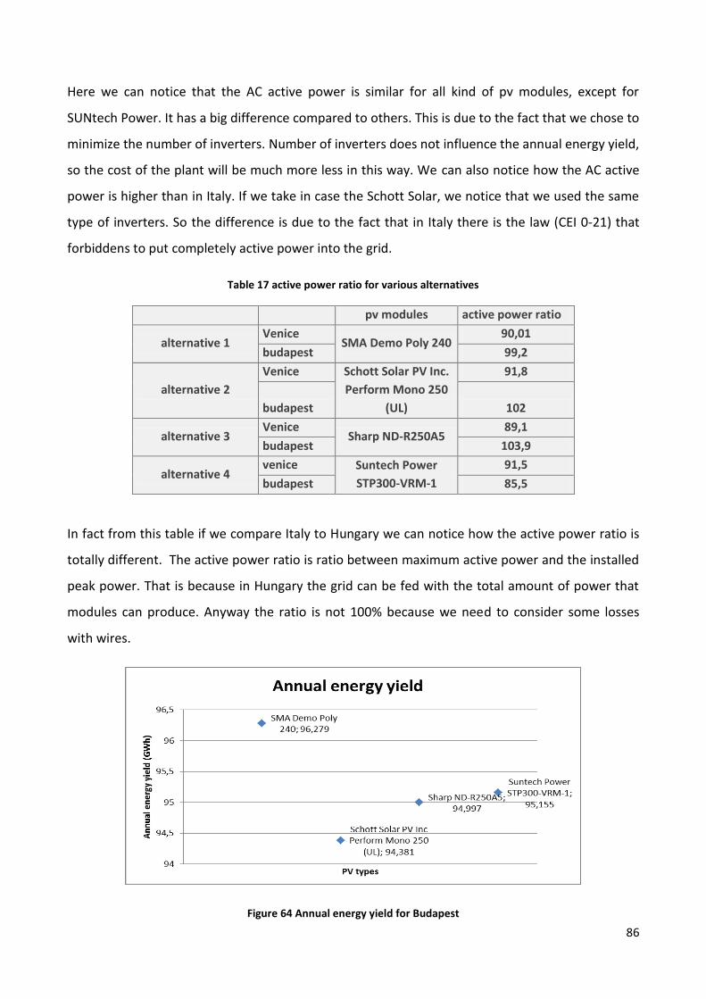
86
Here we can notice that the AC active power is similar for all kind of pv modules, except for
SUNtech Power. It has a big difference compared to others. This is due to the fact that we chose to
minimize the number of inverters. Number of inverters does not influence the annual energy yield,
so the cost of the plant will be much more less in this way. We can also notice how the AC active
power is higher than in Italy. If we take in case the Schott Solar, we notice that we used the same
type of inverters. So the difference is due to the fact that in Italy there is the law (CEI 0-21) that
forbiddens to put completely active power into the grid.
Table 17 active power ratio for various alternatives
pv modules active power ratio
alternative 1 Venice
SMA Demo Poly 240 90,01
budapest 99,2
alternative 2
Venice Schott Solar PV Inc.
Perform Mono 250
(UL)
91,8
budapest 102
alternative 3 Venice
Sharp ND-R250A5 89,1
budapest 103,9
alternative 4 venice Suntech Power
STP300-VRM-1
91,5
budapest 85,5
In fact from this table if we compare Italy to Hungary we can notice how the active power ratio is
totally different. The active power ratio is ratio between maximum active power and the installed
peak power. That is because in Hungary the grid can be fed with the total amount of power that
modules can produce. Anyway the ratio is not 100% because we need to consider some losses
with wires.
Figure 64 Annual energy yield for Budapest

87
Also here we can notice how SMA Demo Poly has the best annual energy yield. The reason is the
same of the Italian case. Inverters we can choose in the software are just made by SMA, so it is
obvious they have the best matching. Schott Solar still remains the worst choice for this type of
plant.
Figure 65 Performance ratio for Budapest
Same as before, the best permormace is given by SMA Demo Poly, which has 89,3%. This amount
is a good result.
Figure 66 Specific energy yield for Budapest

88
SMA Demo Poly is the best also in this case. It means that with the same amount of energy from
the light modules convert into electric energy in the best way, with minus losses than other types
of modules.
9.4 Costs of the plants
For each alternative case examined above we tried to estimate the initial investement required
to build the plants. Besides we tried to figure out annual fixed costs and consider the payback time
for the plants.
We begin by reporting some market prices for modules, inverters and other hardware stuffs.
Modules
SMA Demo Poly 240: 340 €
Schott Solar PV Mono 250: 320 €
Sharp ND-R250A5: for this module we found two market prices, one for West Europe, precisely
from Germany, and one from a company established in Hungary. We quote the two prices
because the difference is remarkable, as well as the price of retail electricity with average
European price. The price from the German factory is 352 €, while from the Hungarian factory is
246 €, both comprehensive of taxes.
Suntech Power STP300-VRM-1: 280 €
Inverters:
MLX60: 9590 €
STP25000TL-30: 5127 €
Miscellaneous components:
SMA sensor box monitoring: 412 €
SMA CLCON-10 Cluster Controller: 1339 €
Speedwire/Webconnect: 150 €

89
Some prices were in dollars; they were converted in Euro using the exchange rate of 1 €= 1.18 $
Due to the big amount of materials we use economy of scale for each component. We decide to
apply a discount between 20% and 40% in order to reach the actual standard cost for a whole PV
system, which is essentially 1.5 €/Wp.
Besides, as we found a remarkable difference in the price between Italy and Hungary, we decided
to cut prices for each component for the Hungarian plant.
Furthermore, to calculate costs of planning and installation and annual fixed costs we used the
percentage shown in the previous graphic in the cost analysis chapter.
The sum of costs for the Italian plant is shown below for every alternative.
Table 18 Sum of costs for Italian plant
Italy Alternative 1 Alternative 2 Alternative 3 Alternative 4
Cost of the PV modules
(M€) 66.682 64.014 67,384 46.326
Cost of inverters (M€) 10.122 10.314 10.008 10.272
PV system monitoring
(M€) 7425 7.102 7.218 6.954
Planning and installation
(M€) 38.855 37.061 39.011 26.820
Total investment (M€) 122.558 118.490 123.603 90.372
Specific capital
expenditure (k€/kWp) 1.455 1.406 1.467 1.072
Annual energy yield
(GWh) 110.77 108.59 109.29 109.58
Annual fixed costs (M€) 4.611 4.611 4.611 4.611
For Hungary instead costs are the following
Table 19 Sum of costs for Hungarian plant
Hungary Alternative 1 Alternative 2 Alternative 3 Alternative 4
Cost of the PV modules
(M€) 46.677 44.809 47.168 32.428
Cost of inverters (M€) 7.08540 7.219 7.005 7.190

90
PV system monitoring
(M€) 5.197 4.971 5.052 4.867
Planning and installation
(M€) 27.198 25.942 27.307 18.774
Total investment (M€) 89.386 86.171 89.762 66.488
Specific capital
expenditure (k€/kWp) 1.061 1.023 1.065 0.789
Annual energy yield
(GWh) 96.279 94.381 94.997 95.155
Annual fixed costs (M€) 2.305 2.305 2.305 2.305
Thanks to the software Matlab we found the total revenue from grid feed-in and the payback time
of the plant by this script:
%Revenues and payback time for a PV plant%
fit=input ('insert feed-in tariff (€/KWh) ') tic=input('insert total investment costs (M€) ') afc=input('insert annual fixed costs (M€) ') initialany=input('inserire annual energy yield (GWh) ') any=0 n=1 y=0 any1=0 while y<1
if any1==0 any1=0 else any=any1 end
any1=any+initialany*0.995^n
afc1=afc*n
revenue=fit*any1*1000000
costs=afc1*1000000+tic*1000000
e1=(revenue-costs)
if e1<0 y1=0
else y1=1 end y=y1 rev (n)=[revenue] cost (n)=[costs] e (n)=[e1] ns (n)=[n]
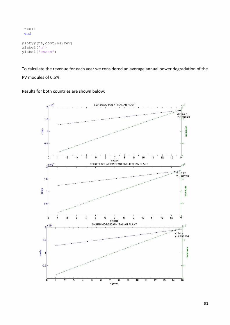
91
n=n+1 end
plotyy(ns,cost,ns,rev) xlabel('n') ylabel('costs')
To calculate the revenue for each year we considered an average annual power degradation of the
PV modules of 0.5%.
Results for both countries are shown below:

92
Figure 67 Payback time for Italian plants

93
Figure 68 Payback time for Hungarian plants
The sum of results is:
Table 20 Sum of payback time period for each alternative
Venice Budapest
Alt. 1 Alt. 2 Alt. 3 Alt. 4 Alt. 1 Alt. 2 Alt. 3 Alt. 4
Payback time (years) 13.87 13.82 14.3 10.25 20.06 19.92 20.6 14.91
9.5 Differences between Venice and Budapest
First of all we need to say that these cities are situated in different parallels. In fact Venice is in the
45° parallel, Budapest is 47°. That means different temperature during the year, but most
important different global radiation. Hereunder we can see differences in these diagrams.
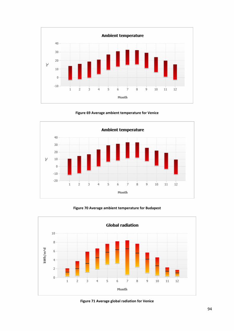
94
Figure 69 Average ambient temperature for Venice
Figure 70 Average ambient temperature for Budapest
Figure 71 Average global radiation for Venice

95
Figure 72 Average global radiation for Budapest
For temperature we can notice that in Venice it is generally higher than in Budapest. In fact,
temperature parameters commonly used are 3:
Annual extreme low temperature (Venice:-4° , Budapest:-14°)
Average high temperature (Venice:23° , Budapest:22°)
Annual extreme high temperature (Venice:33° , Budapest:34°)
This is reflected in the annual global radiation. In Venice it is 1,326.29 kWh/m²a, whereas in
Budapest it 1,203.99 kWh/m²a. This means that there is less energy available in Budapest.
We can notice this in the graphic of annual energy yield and specific energy yield. For example if
we take the SMA modules the annual energy yield for Venice is 110.77 GWh and for Budapest is
96,279 GWh. There is a difference of 14,491 GWh and it is a considerable amount. In Budapest we
can collect the 86.9 % of energy that we can take in Venice. Also if we consider the case of Schott
Solar PV INC modules in which we used the same type of inverter the annual energy yield is totally
different: for Venice is 108,94 and for Budapest is 94,38 GWh. Same reason is for the specific
energy yield.
Another difference between the two cities is the current regulations. As I quoted before in Italy
there is a rule named CEI 0-21 that prohibits the use of inverters for more than 6 KWp. This rule
does not exist in Hungary, so we can use different types of inverters there. That allows money
saving and use of fewer inverters. One example is with SMA modules. For Italy we had to choose
the STP25000TL-30 inverter, instead of MLX 60 inverter for Budapest. In Italy we had to use 3375

96
of that type of inverter, counter just 1394 in Budapest. The first costs 7300 $, the second 9800 $.
In this way in Hungary we can save a lot of money and space also. Probably this rule is used just for
private users who have a small amount of extra energy to feed the grid, but our software cannot
recognize differences between types of installation. Another consideration is that for a big plant
like that we do not use this type of inverters, but usually we use central like SC 630HE which is
functionally in the Montalto di Castro power plant. Its nominal power DC reaches 642 KW, more
than 10 times of MLX60 and 25 times of STP25000TL-30. In this way we can achieve better results,
in terms of both economy and energy. We do not know why the software does not take into
account this possibility, but for our purpose it is not necessary.
Another interesting aspect to notice is that the performance ratio is a little bit higher for
Budapest.
Table 21 Performance ratio for various alternatives
pv modules
performance
ratio
alternative 1 venice SMA Demo Poly
240
89,3
budapest 89,4
alternative 2 venice Schott Solar PV Inc
Perform Mono 250
(UL)
87,4
budapest 87,6
alternative 3 venice
Sharp ND-R250A5 88,1
budapest 88,2
alternative 4 venice Suntech Power
STP300-VRM-1
88,3
budapest 88,3
From the table above we can notice really small differences, except for the Suntech Power
modules. Probably the reason resides in the choice of inverters. Laws in Hungary are less
restrictive and they allow to feed the grid with 100% of the power that came from modules and
using a displacement power factor equal to cosφ=1. As we said before, that permits the use of
bigger capacity inverters which results in a better performance.
Another interesting point to focus is the use of mounting degree. To calculate the best degree we
need to consider essentially two factors: latitude and energy demand.
With latitude we can estimate the best angle for summer, winter, spring and autumn season. A
simple way, but not the most accurate, is the following. For the 21 of March and for the 21 of
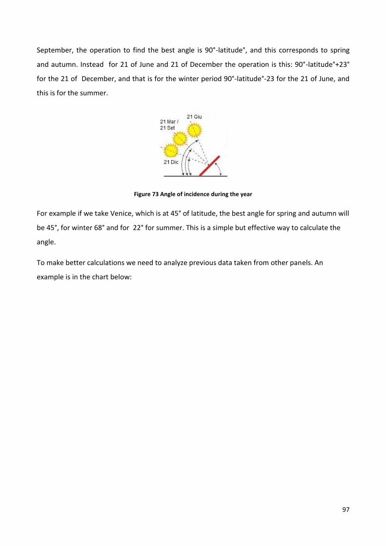
97
September, the operation to find the best angle is 90°-latitude°, and this corresponds to spring
and autumn. Instead for 21 of June and 21 of December the operation is this: 90°-latitude°+23°
for the 21 of December, and that is for the winter period 90°-latitude°-23 for the 21 of June, and
this is for the summer.
Figure 73 Angle of incidence during the year
For example if we take Venice, which is at 45° of latitude, the best angle for spring and autumn will
be 45°, for winter 68° and for 22° for summer. This is a simple but effective way to calculate the
angle.
To make better calculations we need to analyze previous data taken from other panels. An
example is in the chart below:
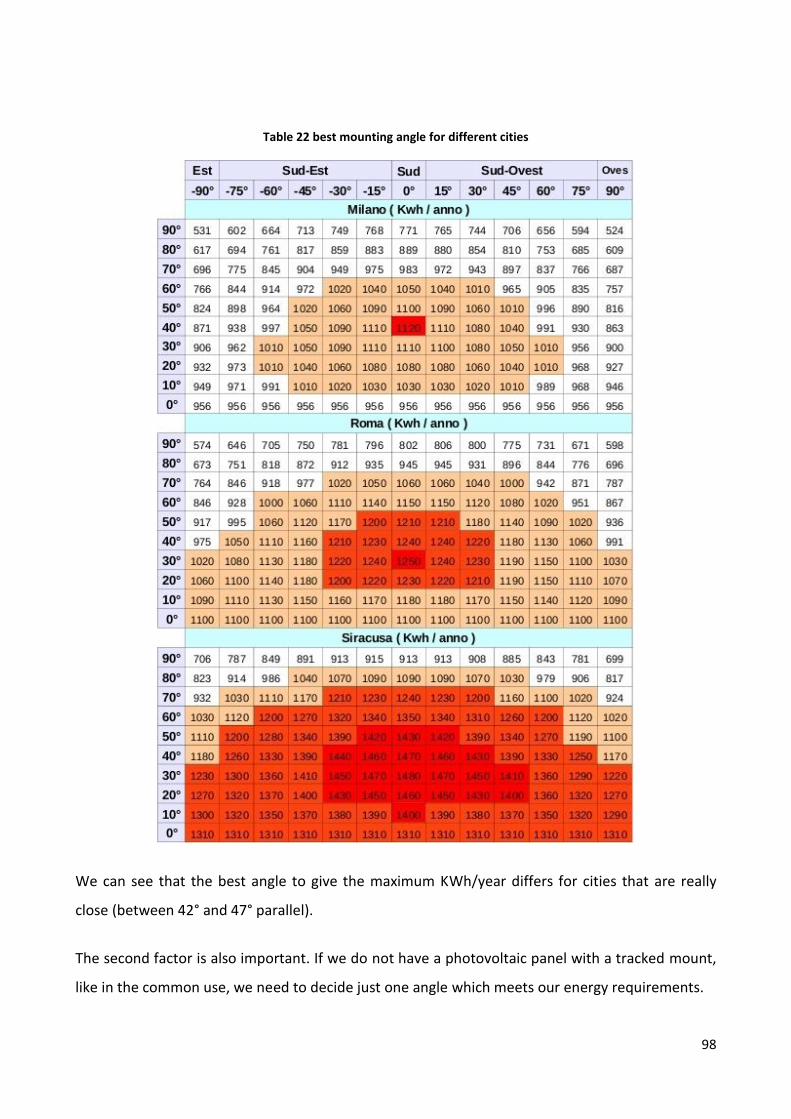
98
Table 22 best mounting angle for different cities
We can see that the best angle to give the maximum KWh/year differs for cities that are really
close (between 42° and 47° parallel).
The second factor is also important. If we do not have a photovoltaic panel with a tracked mount,
like in the common use, we need to decide just one angle which meets our energy requirements.

99
The software loads automatically 35° degrees for Budapest. The best angle for spring and autumn
is 43° degrees. It probably means that in Budapest energy requirements are a little bit higher
during the summer period, instead of in Venice, in which the software chooses 45° degrees. Also
the weather during the year contributes to the choice.
So in our case we used 45° for both cities, maximizing Venice. If we had used the best mounting
angle for Budapest we could have noticed a small difference in the annual energy yield, but still
remarkable. The amount would be 2 GWh more and less, which are enough to meet the energy
needs of two average Swedish towns with a population of 100,000 for 8 hours.
One last consideration to make is about costs, revenues and payback time.
As we said before, Hungary is cheaper than Italy. A discount was required otherwise there would
be no market for PV in Hungary, due to the small economy and the cost of life, which is lower than
in Italy. Therefore, it seemed reasonable to apply a discount up to 25% for each component.
Besides, it seemed reasonable to reduce the annual fixed costs to 50% because manpower is very
cheap in Hungary.
As we can imagine, also the Fit in Hungary is lower than in Italy. This means the revenue is lower
for an equal power of the plant. In fact, the Fit used for Italy was 0.126 €/KWh, for Hungary was
0.074 €/kWh.
Anyway results showed what we expected. In Italy, due to laws, economic benefits and higher
sunlight, PV plants are cheaper. This emerges from the payback time; in Italy the average of
payback time is 14 years, without considering the exceptional value for the technology of the
company SUNTECH POWER (11 years), whereas in Hungary it is 20 years.
The SUNTECH POWER alternative is an exceptional value, due to the 300W modules, instead of
common 240/250W ones, and the cheap price offered to purchase them.

100
10 Software Photovoltaic Geographical Information System
10.1 Overview of the application
This is not a real software, but this is more an interactive map of Europe in which we can estimate
performance of grid-connected photovoltaic. We can also calculate the monthly radiation and the
daily radiation of a precise place.
Figure 74 Photovoltaic Geographical Information System Web application
The System provides 2 different types of climate database.
They are the Climate-SAF PVGIS or the Classic PVGIS. PVGIS needs data on solar radiation in order
to make estimates of the performance of PV systems and to do the other calculations possible in
the web application. There exist a number of different sources of solar radiation data, but none of
them are perfect, so it is important to understand the strengths and weaknesses of each data
source.
Types of solar radiation data sources
The two main sources of data on solar radiation on the surface of the earth are:
Ground measurements

101
Calculations based on satellite data
10.1.1 Ground measurements of solar radiation
Direct measurements of the solar radiation at ground level can be made with a number of
different instruments. A widely used instrument is the pyranometer. Typically, the instrument
measures all the radiation coming from the sun and from the sky or clouds. When you want to
know the solar radiation at a specific place, ground station measurements give the best results. It
is also possible to measure with a high time resolution, typically every minute or even more often.
Anyway, problems with the measurements could arise, when for example the sensor may be
covered with dirt, frost, snow, or it is shadowed by nearby trees or buildings for some time during
the year. These problems can be removed by careful siting and maintenance, but it makes it more
uncertain to use data where you do not have direct experience with the measurements.
10.1.2 Solar radiation estimates from satellite
There are a number of methods to estimate the solar radiation at ground level using data from
satellites. Typically the satellites measure the light (visible or infrared) coming from the Earth. This
light is mainly the light reflected from the ground or from clouds. The calculation of the solar
radiation at ground level must therefore be able to take into account the radiation absorbed by
the atmosphere as well as that reflected by clouds.
Different types of satellites can be used to estimate solar radiation. Geostationary weather
satellites take pictures of the Earth at short intervals (every 15 or 30 minutes) so they have a very
good time resolution. However, each pixel in the picture typically represents a rectangle a few km
on each side, so the estimate of solar radiation for each pixel will be the average of such an area.
Polar-orbiting satellites fly closer to the Earth, so the space resolution is better. However, they do
not stay permanently above a particular area, so they are normally able to take only a couple of
pictures a day of a given area. The data used for PVGIS come mainly from geostationary satellites.
The main advantage of satellite-based methods is that they give a fairly uniform coverage of large
areas while ground stations are often very far apart. On the other hand, there are potential
problems also with the satellite methods:

102
Snow on the ground is a special problem for satellite methods, since snow will look very
much like clouds in the satellite images. There are methods to overcome this problem, but
the uncertainty is higher in areas with snow.
In mountain areas one pixel may cover an area with strongly varying altitude. The solar
radiation dependence on altitude is not well represented in the satellite-based
calculations.
When the sun is very low in the sky the calculation from satellite data becomes very
difficult. This can cause problems, in particular in winter at high latitudes.
The quality of satellite-based estimates must be checked by comparison with high-quality ground
station measurements.
10.1.3 PVGIS classic
The original PVGIS radiation database is based on data from the European Solar Radiation Atlas.
The data consist of ground station measurements from about 560 stations in Europe, over the
period 1981 to 1990. Thus, the data are rather old, and there are strong indications that the
climate has changed in the last 25-30 years, affecting also the solar radiation. The station data
have then been used for a mathematical interpolation to give solar radiation values also for the
areas between stations. However, this interpolation is subject to uncertainties. The density of
stations varies strongly in Europe, and the uncertainty can be very high in areas with few stations.
10.1.4 PVGIS-CMSAF
The new database in PVGIS has been calculated from solar radiation data made available by the
Climate Monitoring Satellite Application Facility (CM-SAF). The solar radiation values have been
estimated from satellite images. The data are fairly recent, from 1998 to mid-2010, so there
should not be strong effects of climate change. However, the use of satellite data has its own
problems. The pixel size in the satellite images is about 3-5km, so smaller features such as narrow
mountain valleys cannot be resolved. The computer algorithm that calculates the solar radiation
on the ground may have difficulties in telling the difference between snow and clouds, which can
have a large influence on the result. The CM-SAF team has worked hard to minimize these errors,
but there are still uncertainties.

103
Types of photovoltaic technology
The three types of photovoltaic modules are:
Crystalline Silicon
CIS
CdTe
With the web application we can choose the installed PV peak power and the estimated system
losses, which, in order to simplify our job, we leave at 14%.
Afterwards we can select the mounting position, mounting angle and the azimuth. We can also
select if we want a tracked angle, but for our job and our purpose this is not necessary.
10.2 Purpose of the project
Our purpose with this application is similar to that of the software SMA Sunny Design, that is to
estimate the power produced from a PV plant about 84,23 MW.
As we did before, we choose two different places to put our PV plant.
The first is near Venice and precisely 45°20'48" North, 12°11'36" East, elevation: 0 m a.s.l. The
place is near the beach, in the Laguna of Venice, in which there is a big empty field.
The second is in Budapest 47°13'31" North, 18°45'7" East, elevation: 136 m a.s.l.
The main data for both places are:
Climate-SAF PVGIS
Power plant: 84,23 MW
Angle slope 45°
Angle Azimuth 0
Free-standing mounting
No tracking positions
We select for each place every type of modules, to show the differences between them.
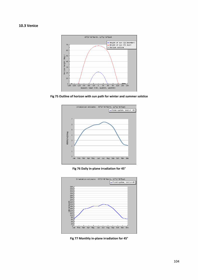
104
10.3 Venice
Fig 75 Outline of horizon with sun path for winter and summer solstice
Fig 76 Daily in-plane irradiation for 45°
Fig 77 Monthly in-plane irradiation for 45°

105
10.3.1 Crystalline Technology
10. TABLE 23 Results for crystalline silicon pv system in Venice
Fixed system: inclination=45 deg.,
orientation=0 deg.
Month Ed Em Hd Hm
Jan 144000
4460000 2.09 64.9
Feb 249000 6970000 3.66 102
Mar 323000 10000000 4.91 152
Apr 350000 10500000 5.43 163
May 367000 11400000 5.86 182
Jun 365000 11000000 5.99 180
Jul 390000 12100000 6.43 199
Aug 376000 11700000 6.16 191
Sep 336000 10100000 5.40 162
Oct 248000 7680000 3.82 119
Nov 159000 4780000 2.39 71.8
Dec 141000 4370000 2.06 63.9
Average
Year 288000 8750000 4.52 138
Total for
year
105000000
1650
Ed: Average daily electricity production from the given system (kWh)
Em: Average monthly electricity production from the given system (kWh)
Hd: Average daily sum of global irradiation per square meter received by the modules of the given
system (kWh/m2)
Hm: Average sum of global irradiation per square meter received by the modules of the given
system (kWh/m2)
In this table the 4 main data of our calculations are shown.
The most important is the total power per year, which is 105 GWh in this case.
Another interesting data is the total sum of global irradiation per square meter received, which is
1650 KWh/m2.
Estimated losses due to temperature and low irradiance: 9.5% (using local ambient temperature)

106
Estimated loss due to angular reflectance effects: 2.7%
Other losses (cables, inverter etc.): 14.0%
Combined PV system losses: 24.3%
Below we can see the trend in graphics of performances of our plant.
Fig 78 Daily energy average output for 45°
Fig 79 Monthly energy output for 45°
We can notice how the trend from January to July more and less rises, after that it starts to lower.
This is completely normal and makes sense, because we select a place in the northern
hemisphere, which means seasons with the summer as the most irradiated. The top of
accumulated energy is in July, when the maximum monthly irradiation occurs.
10.3.2 CIS technology
Estimated losses due to temperature and low irradiance: 8.0% (using local ambient temperature)
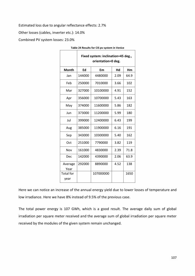
107
Estimated loss due to angular reflectance effects: 2.7%
Other losses (cables, inverter etc.): 14.0%
Combined PV system losses: 23.0%
Table 24 Results for CIS pv system in Venice
Fixed system: inclination=45 deg.,
orientation=0 deg.
Month Ed Em Hd Hm
Jan 144000 4480000 2.09 64.9
Feb 250000 7010000 3.66 102
Mar 327000 10100000 4.91 152
Apr 356000 10700000 5.43 163
May 374000 11600000 5.86 182
Jun 373000 11200000 5.99 180
Jul 399000 12400000 6.43 199
Aug 385000 11900000 6.16 191
Sep 343000 10300000 5.40 162
Oct 251000 7790000 3.82 119
Nov 161000 4830000 2.39 71.8
Dec 142000 4390000 2.06 63.9
Average
Year
292000 8890000 4.52 138
Total for
year
107000000 1650
Here we can notice an increase of the annual energy yield due to lower losses of temperature and
low irradiance. Here we have 8% instead of 9.5% of the previous case.
The total power energy is 107 GWh, which is a good result. The average daily sum of global
irradiation per square meter received and the average sum of global irradiation per square meter
received by the modules of the given system remain unchanged.

108
Fig 80 Daily energy average output for 45°
Fig 81 Monthly energy output for 45°
10.3.3 CdTe technology
Estimated losses due to temperature and low irradiance: 1.2% (using local ambient temperature)
Estimated loss due to angular reflectance effects: 2.7%
Other losses (cables, inverter etc.): 14.0%
Combined PV system losses: 17.4%
TABLE 25 Results for CdTe pv system in Venice
Fixed system: inclination=45 deg.,
orientation=0 deg.
Month Ed Em Hd Hm
Jan 152000
4710000 2.09 64.9
Feb 264000
7380000 3.66 102
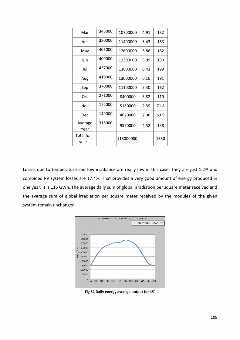
109
Mar 345000
10700000 4.91 152
Apr 380000
11400000 5.43 163
May 405000
12600000 5.86 182
Jun 409000
12300000 5.99 180
Jul 437000
13600000 6.43 199
Aug 419000
13000000 6.16 191
Sep 370000
11100000 5.40 162
Oct 271000
8400000 3.82 119
Nov 172000
5150000 2.39 71.8
Dec 149000
4620000 2.06 63.9
Average
Year
315000
9570000 4.52 138
Total for
year 115000000 1650
Losses due to temperature and low irradiance are really low in this case. They are just 1.2% and
combined PV system losses are 17.4%. That provides a very good amount of energy produced in
one year. It is 115 GWh. The average daily sum of global irradiation per square meter received and
the average sum of global irradiation per square meter received by the modules of the given
system remain unchanged.
Fig 82 Daily energy average output for 45°
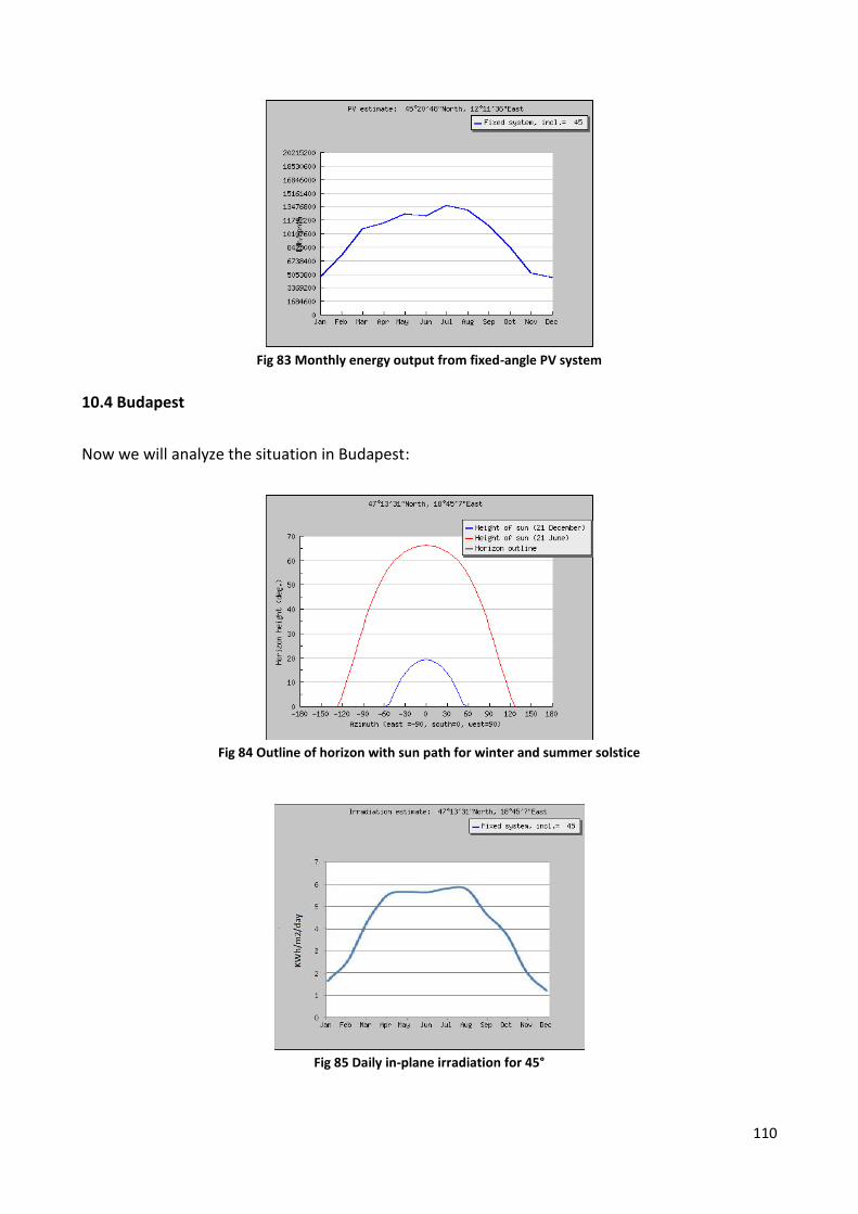
110
Fig 83 Monthly energy output from fixed-angle PV system
10.4 Budapest
Now we will analyze the situation in Budapest:
Fig 84 Outline of horizon with sun path for winter and summer solstice
Fig 85 Daily in-plane irradiation for 45°

111
Fig 86 Monthly in-plane irradiation for 45°
10.4.1 Crystalline silicon technology
Table 26 Results for crystalline silicon pv system in Budapest
Fixed system: inclination=45 deg.,
orientation=0 deg.
Month Ed Em Hd Hm
Jan 118000
3660000 1.66 51.5
Feb 178000
5000000 2.55 71.5
Mar 289000
8970000 4.33 134
Apr 353000
10600000 5.50 165
May 351000
10900000 5.65 175
Jun 346000
10400000 5.63 169
Jul 354000
11000000 5.81 180
Aug 354000
11000000 5.77 179
Sep 295000
8850000 4.64 139
Oct 247000
7650000 3.74 116
Nov 139000
4180000 2.04 61.2
Dec 85500 2650000 1.21 37.4
Average
Year 260000 7900000 4.05 123
Total for
year 94700000 1480
Estimated losses due to temperature and low irradiance: 8.8% (using local ambient temperature)

112
Estimated loss due to angular reflectance effects: 2.8%
Other losses (cables, inverter etc.): 14.0%
Combined PV system losses: 23.7%
Fig 87 Daily energy average output for 45°
Fig 88 Monthly energy average output for 45°
10.4.2 CIS technology
Estimated losses due to temperature and low irradiance: 7.4% (using local ambient temperature)
Estimated loss due to angular reflectance effects: 2.8%
Other losses (cables, inverter etc.): 14.0%
Combined PV system losses: 22.6%
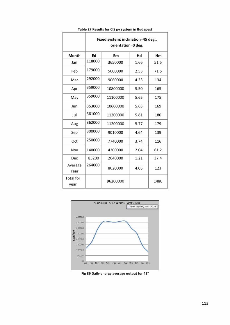
113
Table 27 Results for CIS pv system in Budapest
Fixed system: inclination=45 deg.,
orientation=0 deg.
Month Ed Em Hd Hm
Jan 118000
3650000 1.66 51.5
Feb 179000
5000000 2.55 71.5
Mar 292000
9060000 4.33 134
Apr 359000
10800000 5.50 165
May 359000
11100000 5.65 175
Jun 353000 10600000 5.63 169
Jul 361000
11200000 5.81 180
Aug 362000
11200000 5.77 179
Sep 300000
9010000 4.64 139
Oct 250000
7740000 3.74 116
Nov 140000 4200000 2.04 61.2
Dec 85200 2640000 1.21 37.4
Average
Year
264000
8020000 4.05 123
Total for
year 96200000 1480
Fig 89 Daily energy average output for 45°

114
Fig 90 Monthly energy average output for 45°
10.4.3 CdTe technology
Estimated losses due to temperature and low irradiance: 0.4% (using local ambient temperature)
Estimated loss due to angular reflectance effects: 2.8%
Other losses (cables, inverter etc.): 14.0%
Combined PV system losses: 16.7%
Table 28 Results for CdTe pv system in Budapest
Fixed system: inclination=45 deg.,
orientation=0 deg.
Month Ed Em Hd Hm
Jan 123000 3810000 1.66 51.5
Feb 187000 5230000 2.55 71.5
Mar 308000 9550000 4.33 134
Apr 384000 11500000 5.50 165
May 390000 12100000 5.65 175
Jun 387000 11600000 5.63 169
Jul 397000 12300000 5.81 180
Aug 396000 12300000 5.77 179
Sep 325000 9760000 4.64 139
Oct 268000 8320000 3.74 116
Nov 148000 4450000 2.04 61.2
Dec 89700.00 2780000 1.21 37.4
Average
Year 284000 8640000 4.05 123
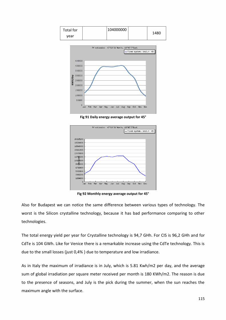
115
Total for
year
104000000
1480
Fig 91 Daily energy average output for 45°
Fig 92 Monthly energy average output for 45°
Also for Budapest we can notice the same difference between various types of technology. The
worst is the Silicon crystalline technology, because it has bad performance comparing to other
technologies.
The total energy yield per year for Crystalline technology is 94,7 GHh. For CIS is 96,2 GHh and for
CdTe is 104 GWh. Like for Venice there is a remarkable increase using the CdTe technology. This is
due to the small losses (just 0,4% ) due to temperature and low irradiance.
As in Italy the maximum of irradiance is in July, which is 5.81 Kwh/m2 per day, and the average
sum of global irradiation per square meter received per month is 180 KWh/m2. The reason is due
to the presence of seasons, and July is the pick during the summer, when the sun reaches the
maximum angle with the surface.

116
10.5 Comparison between Budapest and Italy
The first consideration to make is the difference of radiation. As we supposed the radiation in Italy
is higher. The table below shows the different amount per month.
TABLE 29 Comparison between Venice and Budapest irradiation (kwh/m2)
Month Jan Feb Mar Apr May Jun Jul Aug Sep Oct Nov Dec Year Total for
year
Venice 64.9 102 152 163 182 180 199 191 162 119 71.8 63.9 138 1650
Budapest 51.5 71.5 134 165 175 169 180 179 139 116 61.2 37.4 123 1480
The total amount for Venice is 1650 kWh/m2, instead for Budapest it is 1480 kWh/m2.
The immediate effect is on the production of energy.
Modules can store more energy in Venice.
Another difference, albeit small, is in losses.
For Venice the estimated loss due to angular reflectance effects is 2,7%, instead for Budapest it is
2,8%. This is a really small difference, which probably has not a remarkable effect in the total
energy yield. Something interesting to note instead is the estimated losses due to temperature
and low irradiance.
Table 30 Comparison between Venice and Budapest losses due to temperature and low irradiance
Crystalline
Silicone CIS CdTe
Italy 9,50% 8% 1,20%
Budapest 8,80% 7,40% 0,40%
As we can see there is a small amount of difference, but still remarkable. This is reflected in
combined PV system losses.

117
Table 31 Comparison between Venice and Budapest combined PV system losses
Crystalline
Silicone CIS CdTe
Italy 24,30% 23% 17,40%
Budapest 23,70% 22,60% 16,70%
The smallest difference is in the CIS technology, just 0,4%, but for CdTe technology the difference
is 0,7%, which is not something to give up. CdTe technology is the best technology available, and
also the most inexpensive, so we need to pay more attention to it than to other technologies.
We can say that Budapest has better performance, but this is not enough to contrast the amount
of energy received in Venice. In the end Venice still produces more energy than Budapest.
Another consideration to make, as we made for the software SMA Sunny Design, concerns the
mounting angle. As we said before, the best angle for Venice is about 45°, Budapest around 35°.
We made the same situation in Budapest, changing just the mounting angle with 35°. These are
the results:
Table 32 Results for Silicon Crystalline pv system in Budapest with 35° angle
Fixed system: inclination=35 deg.,
orientation=0 deg.
Month Ed Em Hd Hm
Jan 112000
3460000 1.57 48.7
Feb 172000 4820000 2.46 68.8
Mar 286000
8850000 4.27 132
Apr 359000 10800000 5.59 168
May 368000 11400000 5.91 183
Jun 366000 11000000 5.96 179
Jul 372000 11500000 6.12 190
Aug 364000 11300000 5.93 184
Sep 294000 8820000 4.62 139
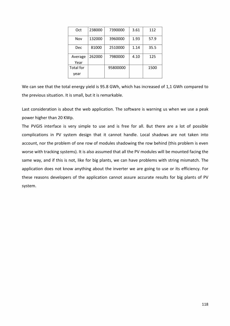
118
Oct 238000 7390000 3.61 112
Nov 132000 3960000 1.93 57.9
Dec 81000 2510000 1.14 35.5
Average
Year
262000 7980000 4.10 125
Total for
year
95800000 1500
We can see that the total energy yield is 95.8 GWh, which has increased of 1,1 GWh compared to
the previous situation. It is small, but it is remarkable.
Last consideration is about the web application. The software is warning us when we use a peak
power higher than 20 KWp.
The PVGIS interface is very simple to use and is free for all. But there are a lot of possible
complications in PV system design that it cannot handle. Local shadows are not taken into
account, nor the problem of one row of modules shadowing the row behind (this problem is even
worse with tracking systems). It is also assumed that all the PV modules will be mounted facing the
same way, and if this is not, like for big plants, we can have problems with string mismatch. The
application does not know anything about the inverter we are going to use or its efficiency. For
these reasons developers of the application cannot assure accurate results for big plants of PV
system.

119
11 Conclusions
As we have seen the use of a PV system of any capacity size is not only economically convenient
but it produces clean energy from renewable source as well. The PV system is environment
friendly due to the fact that it does not produce any CO2 differently from the common fossil fuels.
In fact, during the combustion fossil fuels produce millions of tons of CO2 each year thus polluting
and damaging the Earth through the greenhouse effect. Unfortunately, the fuel based
technologies are still widespread.
However, governments and industry have changed policies so that we can say that nowadays they
aim at producing energy from PV by raising the cumulated capacity of PV plants more and more.
They are trying to reach a higher and higher share of clean energy.
On the other hand, the production of this energy is still considered quite expensive as the overall
efficiency is low. The photovoltaic working system was discovered long time ago (1950s), but this
technology entered the global market view only a few decades ago. It is still a fresh technology, its
development being just at the beginning.
In the next years with advanced researches and investments this field will achieve a full spread in
the world, using more and more conversion efficiency and reducing the costs of plants.
The price of a plant is already competitive, as we showed above (Ch.8) both for residential,
commercial and industrial fields.
It is obvious that a key parameter is the average radiation for a selected zone. In our study we
chose to compare Italy to Hungary, precisely Venice to Budapest. As we know, the average
radiation in Venice is higher than in Budapest due to the latitude, which is lower in Venice than in
Budapest.
As our study demonstrated the annual energy yield, which is the most important data for a PV
power plant, is higher in Venice, and that is solely due to the latitude. The average difference is 14
GWh, which is a remarkable value. Italy has an incredible amount of sunlight and this is one of the
reasons why Italy is the second country in Europe with major installed capacity nowadays. For a
long time Italy brought about a good policy and great FiTs to encourage the use of PV systems. An
important effect was the rapid decrease of the price for a whole PV system, which saw a cut of
half of its price in just 3 years.

120
Taking into account the data from the Montalto di Castro power plant, which was finished in 2010,
we tried to design another one with the same capacity. The total initial investment for our plant
was estimated between 90 and 120 million Euros current price, which is half of the investment in
Montalto di Castro. The payback time is between 11 and 14 years, which is a sustainable value.
For Hungary we did the same study. The total investment was estimated between 65 and 90
million Euros, as the average level of richness is lower than in Italy. The annual fixed costs were
valued in 2.3 million Euros, which are half of the Italian value. Due to the slow policies and not
encouraging FiTs and the less amount of sunlight the payback time in Hungary is between 15 and
20 years, which is estimated too much high, also because FiTs are usually guaranteed for 20 years.
Hungary market in fact seems to be still unsustainable for large scale PV production.
As for the annual energy yield, using the Web application (Ch.9) we could notice basically the same
situation in the two cities. We saw instead differences in the technology used for PV modules. In
fact, for Venice we recorded an annual energy yield of 105 GWh for crystalline silicon, 107 GWh
for CIS technology and 115 GWh for CdTe technology, thus making the efficiency of the latter
much higher than the other two.

121
12 References
Practical handbook of photovoltaics; Fundamentals and applications. Second edition,
AUGUSTIN MCEVOY, TOM MARKVART, LUIS CASTAÑE. 2012 Elsevier Ltd.
Környezettechnika, TERC Kft.Budapest, 2013; Dr. Csoknyai Tamás, Dr. Kircsi Andrea, Dr.
Kalmár Ferenc, Talamon Attila.
National Energy Strategy 2030; Date of Publication: 2012, Publisher: Ministry of National
Development, ISBN 978-963-89328-3-9. Ministry of National Development
Optical gain in silicon nanocrystals L. Pavesi, L. Dal Negro, C. Mazzoleni, G. Franzo, F. Priolo,
Nature 408 (2000)
Renewable Energy Technologies: Cost analysis series, IRENA, 2012
Photovoltaic electricity costs maps, H. Ossenbrink, T. Huld, A. Jäger Waldau, N. Taylor,
European Commission, 2013
Environment, Health and Safety Issues for Sources Used in MOVPE Growth of Compound
Semiconductors. Journal of Crystal Growth
PV in Hungary 2012 - Status Report. Miklós Pálfy
Global Market Outlook for Photovoltaics 2014-2018, EPIA 2014
SUNNY DESIGN 2.20: Software for planning PV plants; User Manual; SDesign-BA-
BEN120432 - Version 3.2
https://solar.org.au
https://terna.it
http://www.iea.org
http://re.jrc.ec.europa.eu/pvgis/apps4/pvest.php
http://www.sma.de/en/products/references/montalto-di-castro.html


![Index [tesi.cab.unipd.it]tesi.cab.unipd.it/47730/1/tesi_Paccagnella_1056656.pdfcultivation activity, management, reclamation of the quarry as well as to the preserving of the territory](https://static.fdocuments.in/doc/165x107/5e5084bf8b30864bcc099439/index-tesicabunipdittesicabunipdit477301tesipaccagnella-cultivation.jpg)