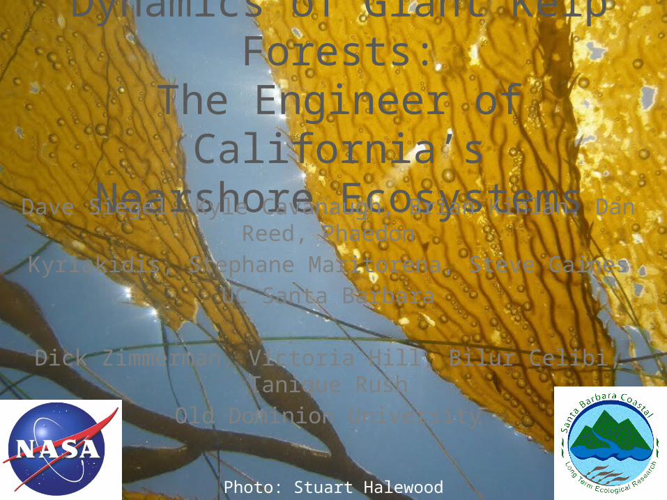
Dynamics of Giant Kelp Forests:The Engineer of California’s

Nearshore EcosystemsDave Siegel, Kyle Cavanaugh, Brian Kinlan, Dan Reed, Phaedon

Kyriakidis, Stephane Maritorena, Steve GainesUC Santa Barbara

Dick Zimmerman, Victoria Hill, Bilur Celibi, Tanique RushOld Dominion University

Photo: Stuart Halewood

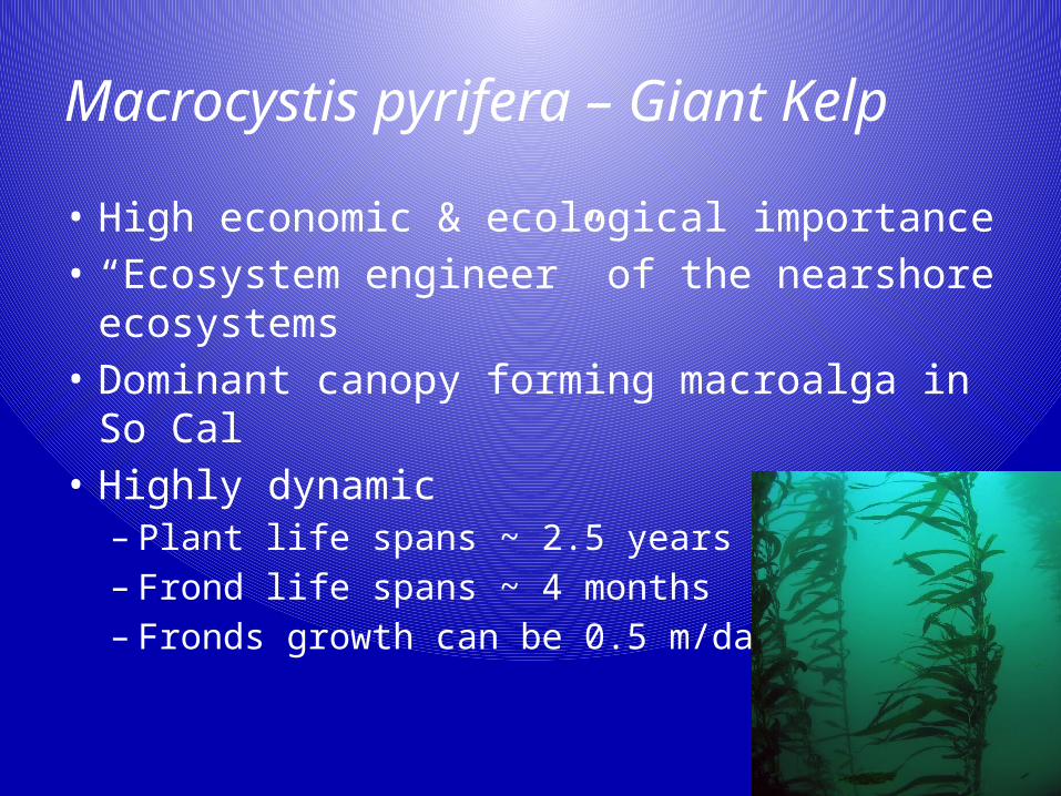
Macrocystis pyrifera – Giant Kelp

• High economic & ecological importance• “Ecosystem engineer” of the nearshore

ecosystems• Dominant canopy forming macroalga in So Cal• Highly dynamic– Plant life spans ~ 2.5 years– Frond life spans ~ 4 months– Fronds growth can be 0.5 m/day

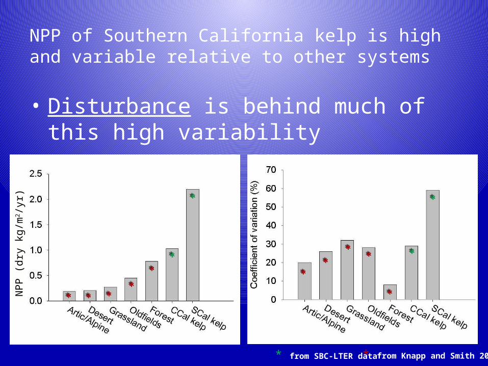
NPP of Southern California kelp is high and variable relative to other systems

• Disturbance is behind much of this high variability

* from Knapp and Smith 2001* from SBC-LTER data

NPP

(dry

kg/

m2 /

yr)

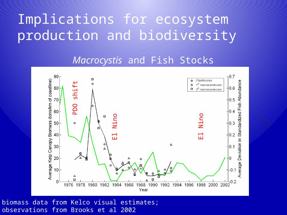
Implications for ecosystem production and biodiversity

Macrocystis and Fish Stocks

Kelp biomass data from Kelco visual estimates;Fish observations from Brooks et al 2002

PDO

shi

ft

El N

ino

El N

ino

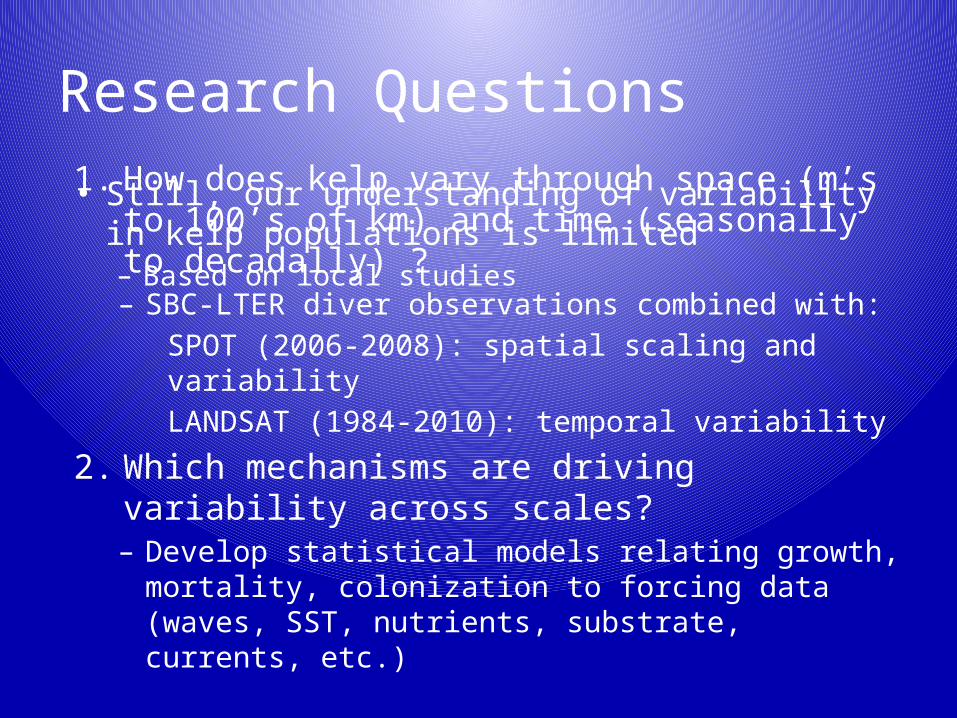
Research Questions1. How does kelp vary through space (m’s to 100’s of

km) and time (seasonally to decadally) ?– SBC-LTER diver observations combined with:

SPOT (2006-2008): spatial scaling and variabilityLANDSAT (1984-2010): temporal variability

2. Which mechanisms are driving variability across scales?– Develop statistical models relating growth, mortality,

colonization to forcing data (waves, SST, nutrients, substrate, currents, etc.)

• Still, our understanding of variability in kelp populations is limited– Based on local studies

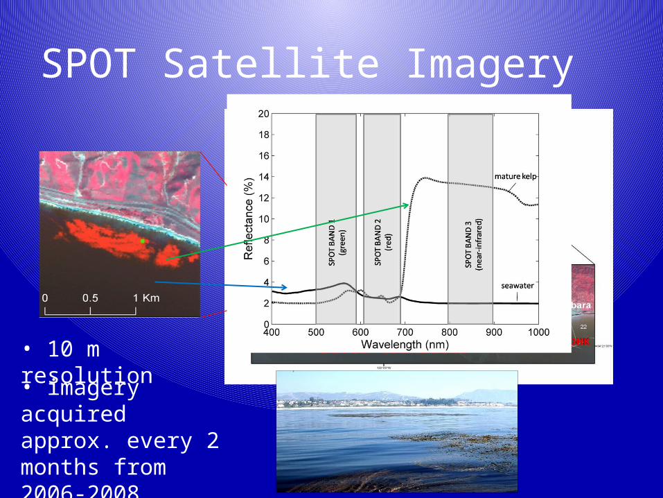
SPOT Satellite Imagery

• imagery acquired approx. every 2 months from 2006-2008

• 10 m resolution Diver transects

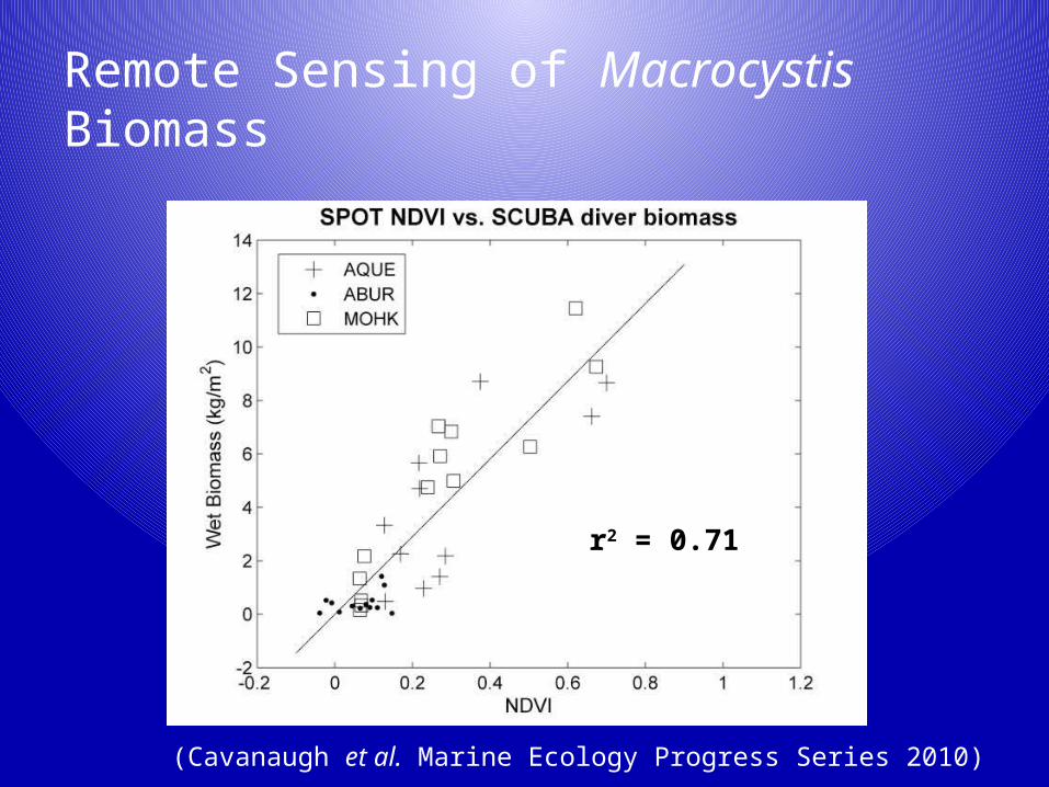
Remote Sensing of MacrocystisBiomass

r2 = 0.71

(Cavanaugh et al. Marine Ecology Progress Series 2010)

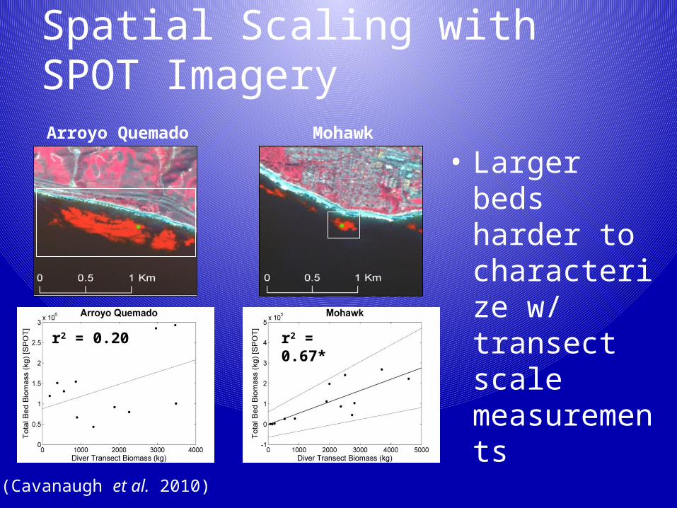
Spatial Scaling with SPOT Imagery

Arroyo Quemado Mohawk

r2 = 0.20 r2 = 0.67*

• Larger beds harder to characterize w/ transect scale measurements

(Cavanaugh et al. 2010)

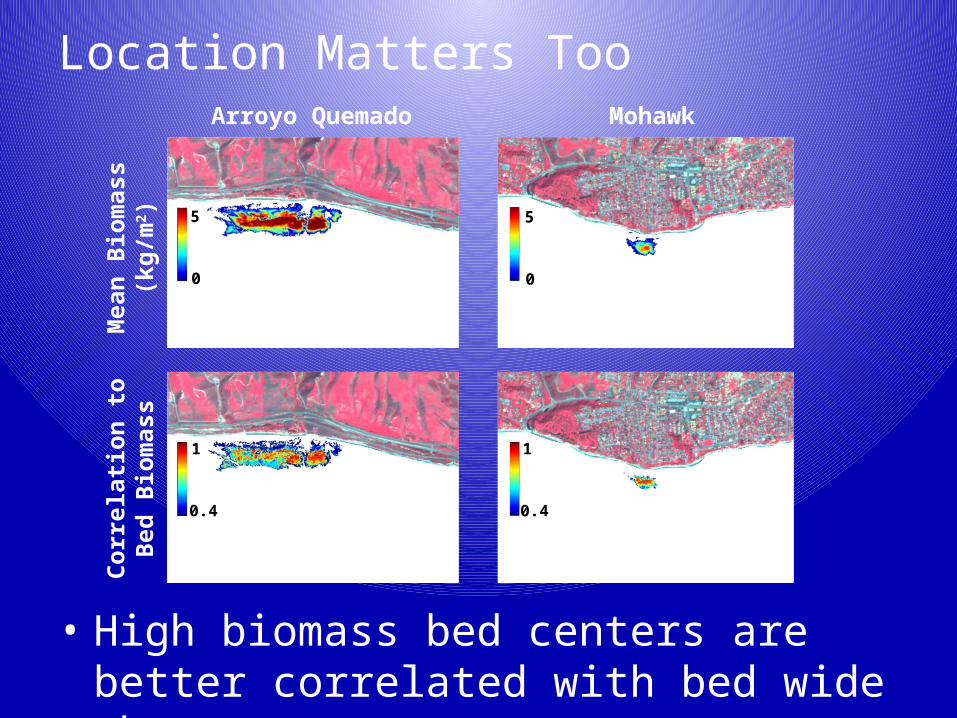
• High biomass bed centers are better correlated with bed wide changes

Arroyo Quemado MohawkM

ean

Biom

ass

(kg/

m2 )

Corr

elati

on to

Bed

Bi

omas

s

Location Matters Too

0

5

0

5

0.4

1

0.4

1

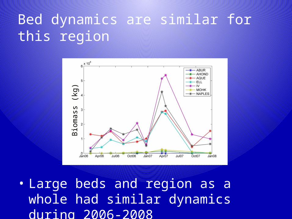
Bed dynamics are similar for this region

• Large beds and region as a whole had similar dynamics during 2006-2008

Biom

ass

(kg)

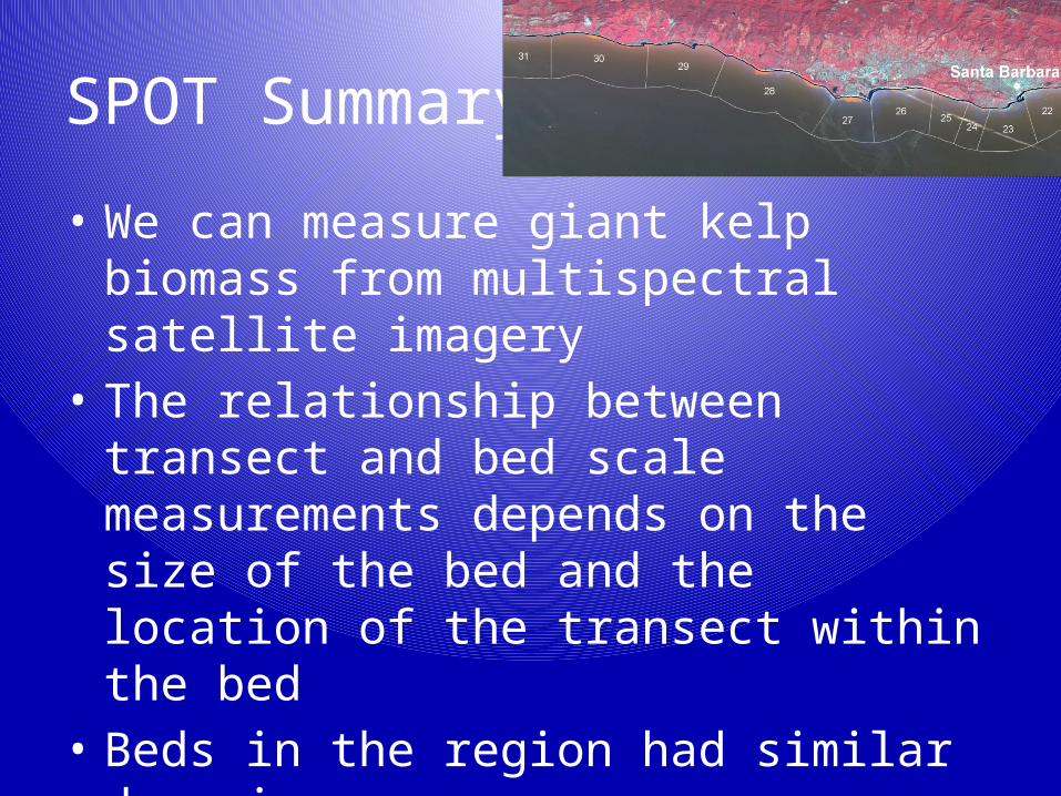
SPOT Summary

• We can measure giant kelp biomass from multispectral satellite imagery

• The relationship between transect and bed scale measurements depends on the size of the bed and the location of the transect within the bed

• Beds in the region had similar dynamics

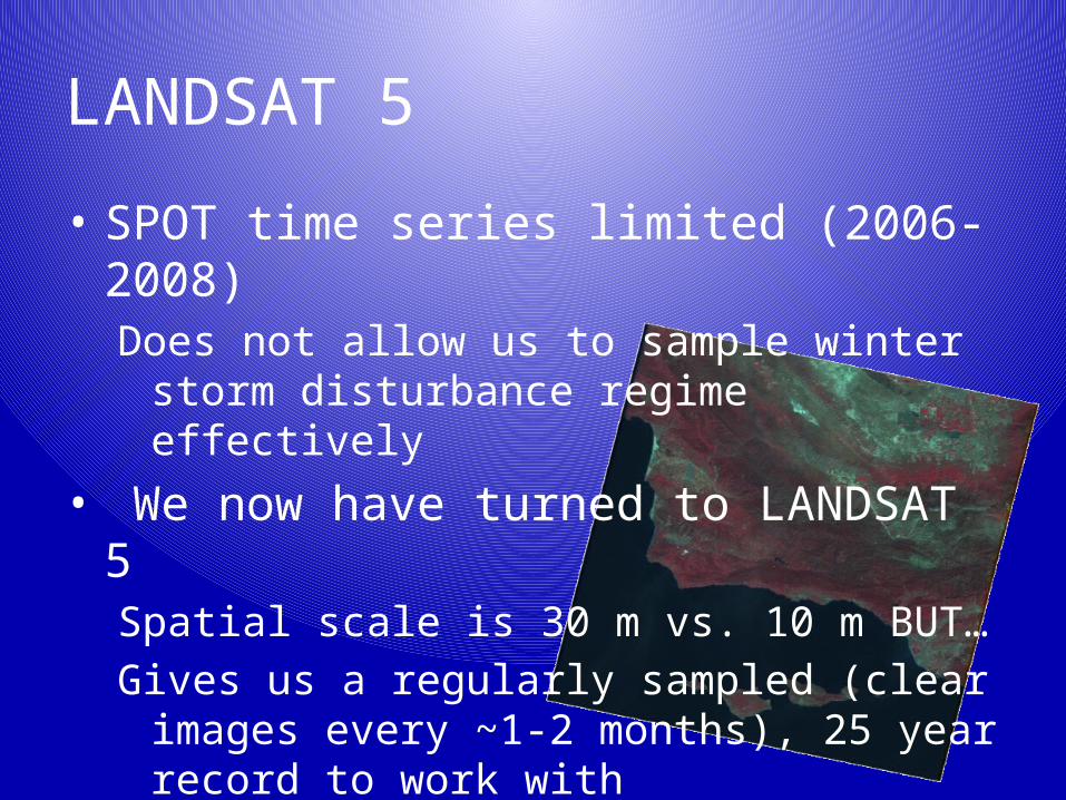
LANDSAT 5

• SPOT time series limited (2006-2008)Does not allow us to sample winter storm

disturbance regime effectively• We now have turned to LANDSAT 5

Spatial scale is 30 m vs. 10 m BUT…Gives us a regularly sampled (clear images every ~1-

2 months), 25 year record to work with

LANDSAT Goals

• Can we get biomass from LANDSAT as we did with SPOT?

• What is driving temporal variability of giant kelp biomass in the Santa Barbara Channel? How is that affecting NPP?

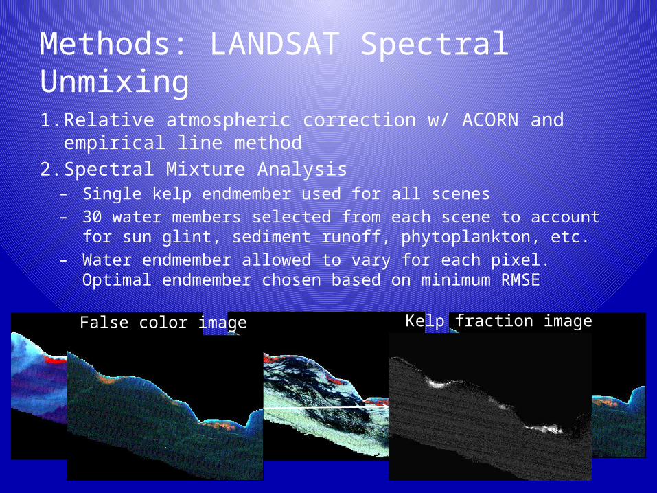
Methods: LANDSAT Spectral Unmixing1. Relative atmospheric correction w/ ACORN and empirical line

method2. Spectral Mixture Analysis

– Single kelp endmember used for all scenes– 30 water members selected from each scene to account for sun glint,

sediment runoff, phytoplankton, etc.– Water endmember allowed to vary for each pixel. Optimal endmember

chosen based on minimum RMSE

False color image Kelp fraction image

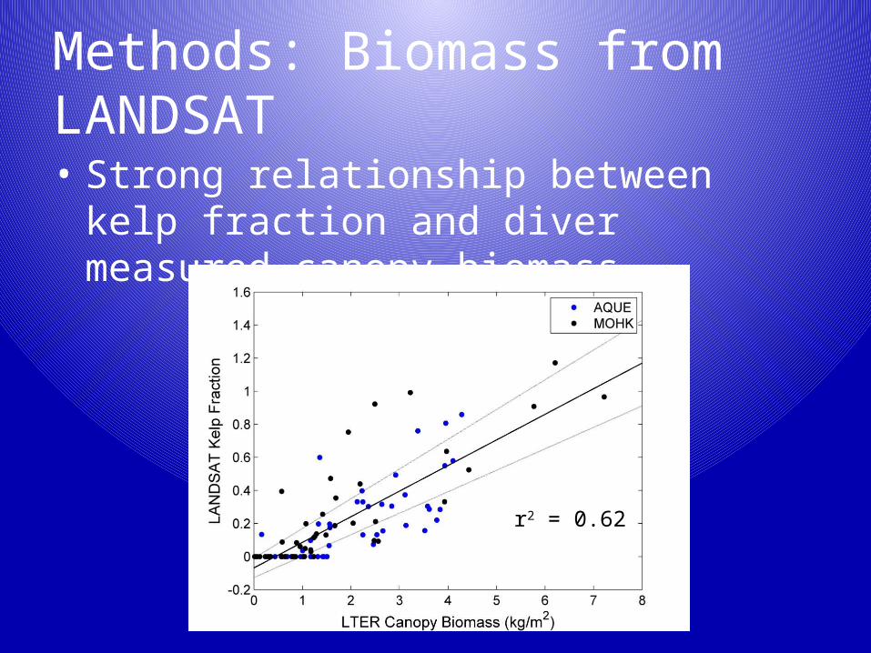
• Strong relationship between kelp fraction and diver measured canopy biomass

Methods: Biomass from LANDSAT

r2 = 0.62

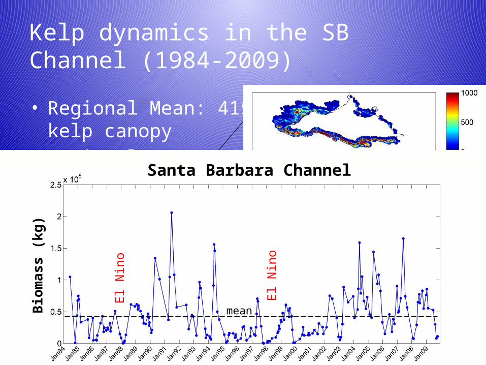
Kelp dynamics in the SB Channel (1984-2009)

• Regional Mean: 41500 metric tons of kelp canopy• Regional CV: 87%

Mean Biomass (kg)

mean

El N

ino

El N

ino

Biom

ass

(kg)

Santa Barbara Channel

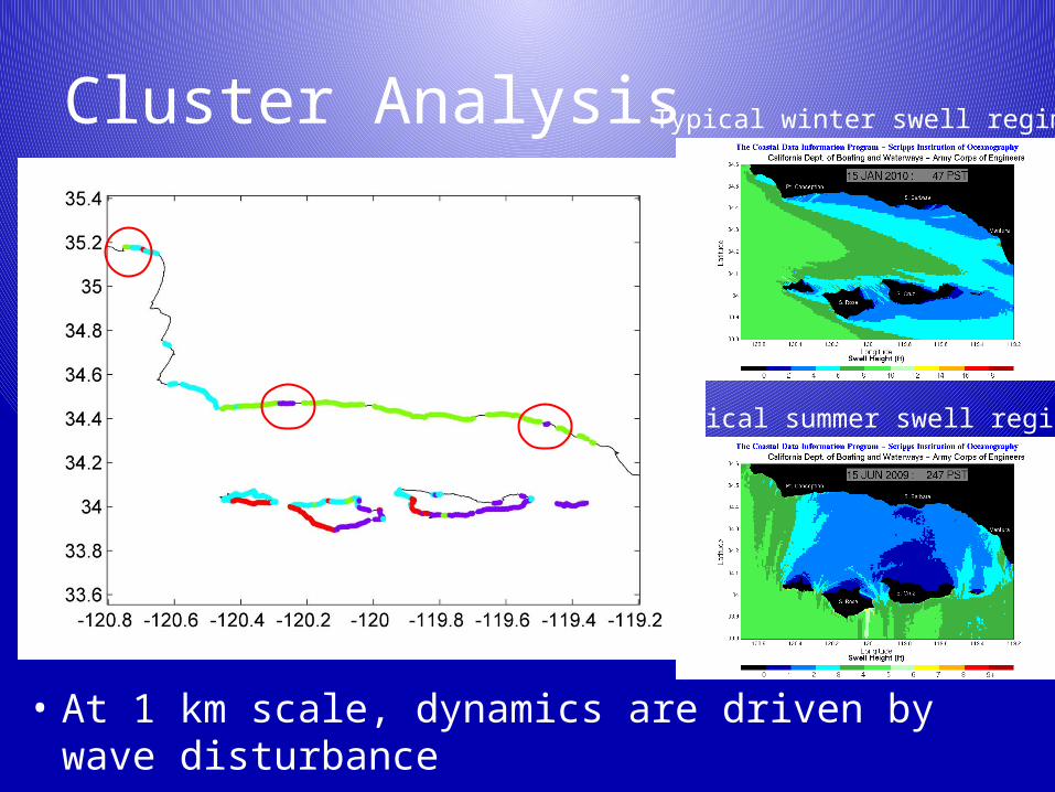
Cluster Analysis

• At 1 km scale, dynamics are driven by wave disturbance

Typical winter swell regime

Typical summer swell regime

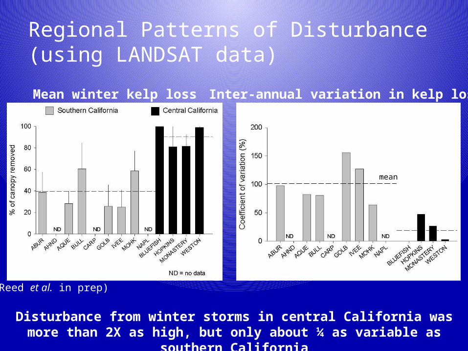
Regional Patterns of Disturbance (using LANDSAT data)

Mean winter kelp loss Inter-annual variation in kelp loss

mean

Disturbance from winter storms in central California was more than 2X as high, but only about ¼ as variable as southern California

(Reed et al. in prep)

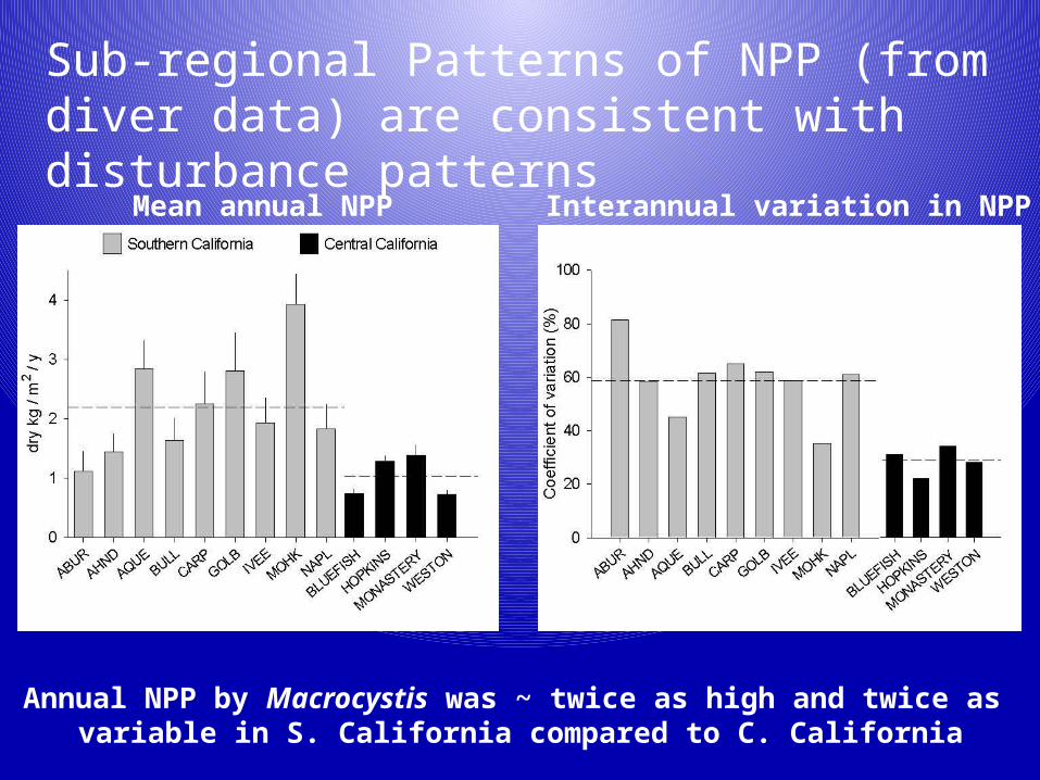
Sub-regional Patterns of NPP (from diver data) are consistent with disturbance patterns

Mean annual NPP Interannual variation in NPP

Annual NPP by Macrocystis was ~ twice as high and twice as variable in S. California compared to C. California

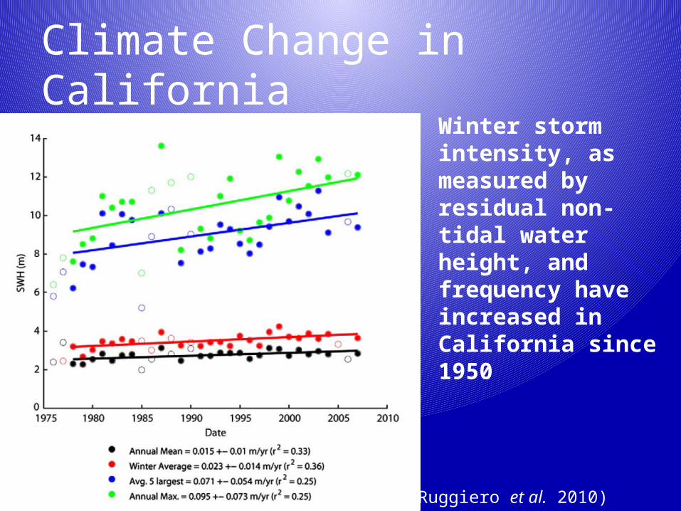
Climate Change in CaliforniaWinter storm intensity, as measured by residual non-tidal water height, and frequency have increased in California since 1950

(Ruggiero et al. 2010)

LANDSAT Summary

• We have created a time series of giant kelp biomass in the Santa Barbara Channel between 1984-2010 with unprecedented spatial and temporal resolution from LANDSAT imagery

• Temporal dynamics at the 1 km scale seem to be driven largely by wave exposure

• Kelp forests in areas with higher wave exposure have lower and less variable NPP

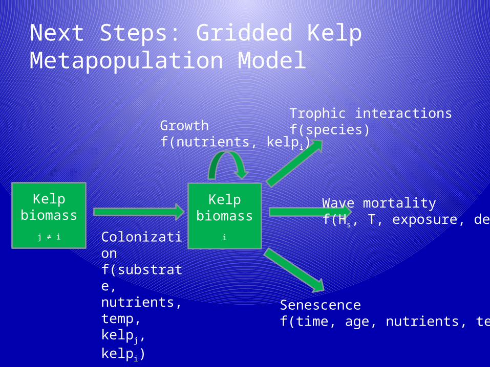
Next Steps: Gridded Kelp Metapopulation Model

Kelp biomass i

Kelp biomass j ≠ i

Trophic interactionsf(species)

Wave mortalityf(Hs, T, exposure, depth)

Senescence f(time, age, nutrients, temp)

Growthf(nutrients, kelpi)

Colonizationf(substrate, nutrients, temp, kelpj,

kelpi)

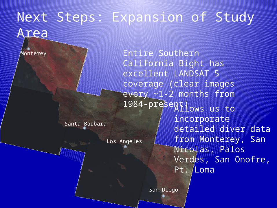
Next Steps: Expansion of Study Area

Entire Southern California Bight has excellent LANDSAT 5 coverage (clear images every ~1-2 months from 1984-present)

Allows us to incorporate detailed diver data from Monterey, San Nicolas, Palos Verdes, San Onofre, Pt. Loma

Santa Barbara

Los Angeles

San Diego

Monterey

Thank You!!