Photo:EmilyArnoldMest

Landscapemetricindicatorsasabaselineforthe

"CaminosdeLiderazgo"Program,Peninsulade

Osa,CostaRica

LuciaMoralesBarquero

April2016

ThisdocumentispartoftheOsaandGolfitoInitiative

Acknowledgments

TheLandSatdataanalyzedforthisreportweredownloadedfromtheUSGeologicalSurveyvia

theGLOVISdataportal (glovis.usgs.gov). TheRapidEyedatawere initiallyprocessedbyEben

Broadbent, PhD, affiliated researcher at Stanford Woods Institute for the Environment

[currentlyco-directorof theSpatialEcologyandConservation(SPEC)Labat theUniversityof

Alabama](seehttp://inogo.stanford.edu/resources/INOGOMapas?language=en).

Funding for this analysis was provided by INOGO (Iniciativa Osa y Golfito) of the Stanford

Woods Institute for the Environment, within the Caminos de Liderazgo Program - a

collaboration insouthernCostaRicabetweenINOGO,theCostaRicaUnitedStatesFoundation

forCooperation,andCostaRica’sNationalSystemofProtectedAreas(SINAC),andimplemented

byRBA(ReinventingBusinessforAll).

Special thanks go toDr. LynneGaffikin, ConsultingAssociateProfessor at StanfordUniversity

andINOGO’sHealthandMetricsAdvisor,forherassistanceinconceptualizingtheanalysisand

overseeing its progress and report finalization. Appreciation is also extended to Ms. Emily

ArnoldMest, INOGO’sAssociateDirector,andMs.MarianaCortésandMs.AnaCamachoofthe

CRUSAFoundationforfacilitatingtheconsultancy.

ThevalidityoftheresultsdocumentedinthisreportcannotbeguaranteedbytheCaminosde

LiderazgoProgram,INOGOortheStanfordWoodsInstitutefortheEnvironmentasthedataand

analyseswereprocessedbythirdparties.

3

Tableofcontents

1.Introduction.......................................................................................................................1

Objective.......................................................................................................................................................................2

Overviewoftheeffectsofecotourismrelatedinterventionsintropicalforests...........................2

Monitoringtourismeffectsonecosystemsthroughlandscapeecology...........................................3

2.Methods...............................................................................................................................5

Studyareadescription............................................................................................................................................5

Datasetsdescription...............................................................................................................................................7

Remotesensinganalysis........................................................................................................................................8

LandscapeMetricAnalysis....................................................................................................................................9

3.Results..................................................................................................................................9

LandcoverandchangeinlandcoverthroughoutfourdecadesintheCaminosfocalarea.....9

Changesinnaturalecosystemsthroughtime............................................................................................12

Comparisonofcurrentstateusinglandscapemetricsatmediumandhighresolution.........15

4.DiscussionandConclusions.....................................................................................19

Conclusions...............................................................................................................................................................20

Outlook.......................................................................................................................................................................21

SupplementaryInformation..............................................................................................................................22

Listoffigures

Figure1ManagementcategorieswithintheCaminosfocalarea..................................................................6

Figure2Outlineof3ofthe5targetedcommunitieswithintheCaminosfocalarea(boundariesdeterminedbyparticipatorymapping)....................................................................................................................7

Figure3LandcoverchangemapfortheCaminosareabetween1975and2000..............................11

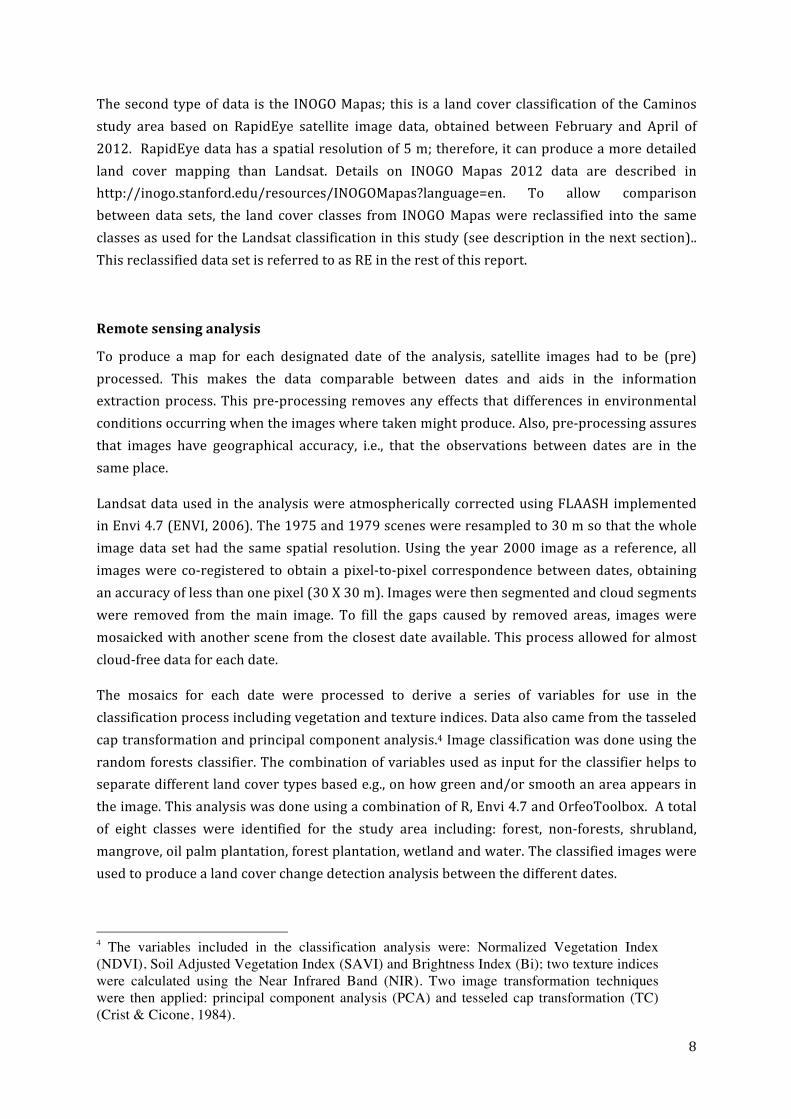
Figure4LandcoverchangemapfortheCaminosfocalareabetween2000and2014...................12

Figure5MainlandscapemetricstodescribepatchdynamicsofthenaturalecosystemswithintheCaminosfocalareathroughtime......................................................................................................................13

Figure6MainlandscapemetricstodescribefragmentationofthenaturalecosystemswithintheCaminosfocalareathroughtime..............................................................................................................................14

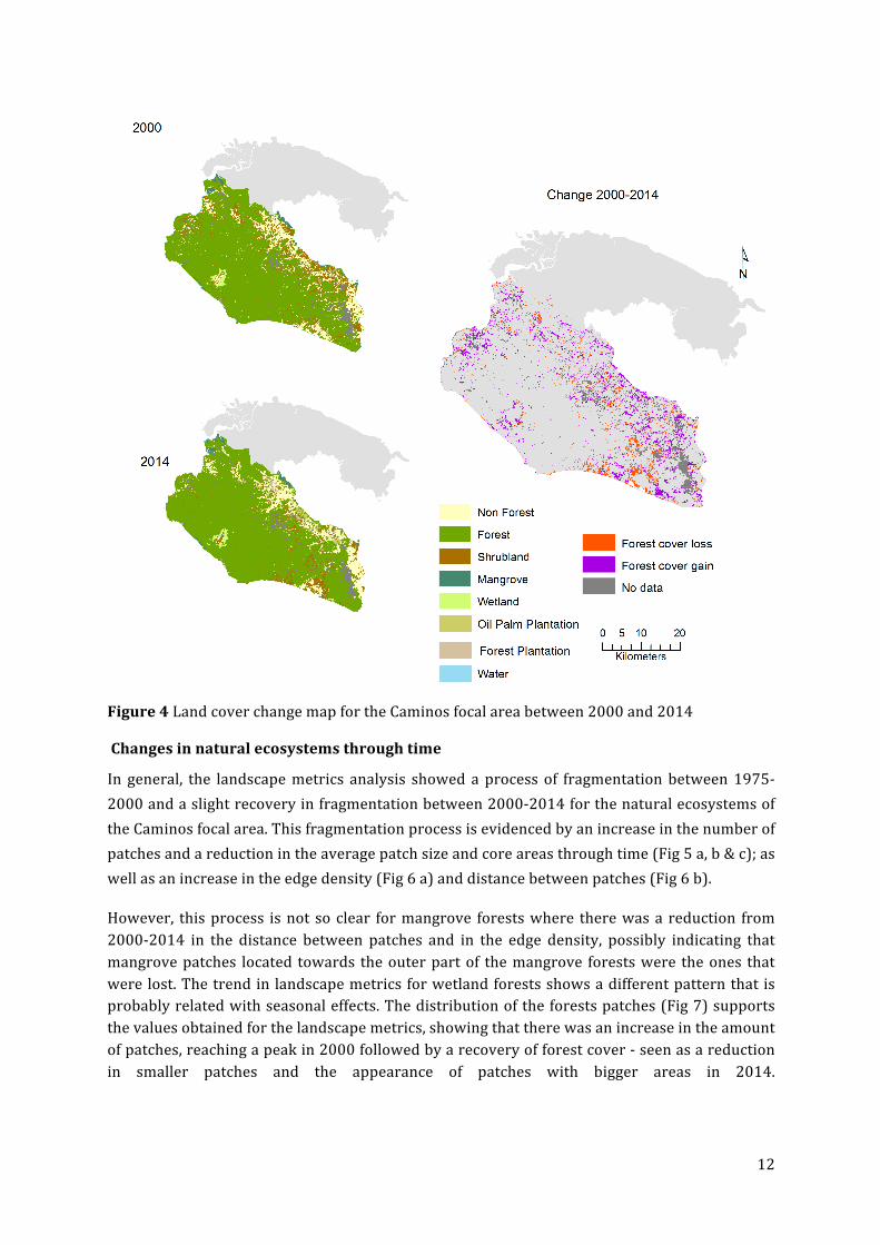
Figure7PatchareadistributionfortheforestclassthroughtimefortheCaminosfocalarea......(Patcharearangeconsidered5-300ha)...............................................................................................................15

Figure 8 Landscapesmetrics for Caminos focal area derived frommaps produced from twodifferentsensors:Landsat8(2014)andRapidEye(2012)andtheresampleto30mofRapidEyedata.........................................................................................................................................................................................17

Listoftables

Table1Satellitedatausedinthestudy(LandsatScenePath54Row14)................................................7

Table2Baseline landcoverbyyear in theCaminos focal area (estimatedbasedondata fromLandsattimeseries).......................................................................................................................................................10

Table3Comparisonbetweenlandcoverclasses(ha)estimatedusingRapidEyeversusLandsat8satellitedata...................................................................................................................................................................16

Table4Comparisonbetween thedistribution andmeanpatch size (ha) forLandsat8 (2014)andRE(2012)datasets................................................................................................................................................18

1

Landscapemetricindicatorsasabaselineforthe"Caminosde

Liderazgo"Program,PeninsuladeOsa,CostaRica

1.Introduction

CaminosdeLiderazgo(hereafterreferredtoasCaminos)isaninitiativethataimstocontribute

to sustainable development in the Osa region. It intends to do so by encouraging

entrepreneurship-based tourism that will improve the socio-economic conditions of local

communities, while trying to maintain the integrity of the natural ecosystems in the region.

Caminos is the result of a unique collaboration between local leaders and entrepreneurs,

CRUSA, the Stanford Woods Institute for the Environment through its INOGO program

(inogo.stanford.edu/), SINAC (National Systemof ConservationAreasofCostaRica), andRBA

(www.grupo-rba.com),withadditionalsupportfromtheprivatesector.1

About 80% of the territory in the Osa Peninsula is under some category of protection

(biodiversity)withvaryinglevelsoflanduserestrictions.Theserestrictionsposealimittothe

typeandextentofeconomicactivitiesthatcanbecarriedoutintheregionthat,tosomeextent,

hascreatedconflictsbetweenthelocalcommunitiesandtheconservationof localecosystems.

In this context, ecotourism can potentially provide an alternative income source to the local

communities.

The backbone of Caminos as a sustainable ecotourism2 initiative is the development of three

trails that cross the Caminos “focal area” (the geographic reach of Caminos effects), where

existingorplannedtouristicactivities(accommodation,restaurants,birdwatching,etc.)willbe

carriedout.Avoidingorminimizingnegative impactsarising fromtheseactivitiesonthe local

ecosystemsisapriorityfortheinitiative.

Thereisrelativelylittleempiricalevidenceontheeffectsthatecotourismmighthaveontropical

forests andwhat,when, and how tomonitor these effects. In thework described herein,we

measure indicators that have been proposed elsewhere to monitor biodiversity in tropical

forestecosystems,asproxiestoassessthecurrentstateoftheecosystemswithintheCaminos

focalarea.Specifically,wedevelopedabaselineorreferencelevelthatservesasabenchmark,to

which any effects that eco-touristic interventions supported by Caminos might have can be

compared.Theindicatorspresentedhereinarelimitedtothosethatcanbemeasuredthrough

remote sensing data that were readily available and could be secondarily analysed for this

exercise. Theseindicatorsarenotintendedasabasisforassessingthesuccessorfailureofany

specificinterventionortheprogressofCaminostowardsachievingaspecificobjective.Rather,

theyservetodocumentthecurrentstateofthenaturalresourcesintheprojectareaandasan

1FurtherinformationonCaminoscanbefoundatwww.caminosdeosa.com.2 The terms ecotourism, sustainable tourismor nature-based tourism are used interchangeably hereinalthoughwerecognizethattherearedifferenceswithinthem.

2

informed basis for understanding how things change over time, associated with ecotourism

interventionsintheareawereCaminosisbeingimplemented.

Objective

Theobjectiveofthisreportistocreatebaselineinformationonthestateofselectedbiodiversity

indicatorswithintheCaminosfocalareaatthebeginningofitsimplementation.

Overviewoftheeffectsofecotourismrelatedinterventionsintropicalforests

Nature-basedtourism,ecotourismorsustainabletourismhavedifferenttypesofimpactsonthe

ecosystems where they are practiced. Those impacts vary depending on the type, intensity,

duration and spatial extent of the various tourism activities. The need to integrate ecological

concepts into ecotourism design, management and impact monitoring has long being

recognized (Newsome et al., 2013). However, there is also a recognition that managing thetourist industry from an ecological perspective is not easy and improvements are urgently

needed, particularly in terms ofmonitoring frameworks (Miller & Twining-Ward, 2005). The

sectionbelowbrieflyprovidessomecontextrelatedtowhattypesofmonitoringhasbeendone

toassesstheeffectsofecotourismintropicalecosystems.

Experiencewithindicatorsbothforevaluatingtheeffectsoftourismontheenvironmentorfor

evaluatingsustainable tourismandecotourismhasbeenratherexploratory.Althoughthere is

clearly a high demand and keen interest to evaluate the effects of tourism industry on the

environment and the conservation of resources, methodological approaches to developing

appropriateindicatorsisinanearlystage(Miller&Twining-Ward,2005).

Mostof thestudies thathaveevaluatedtheeffectsofecotourismonnatureconservation(and

otherenvironmentalchanges)inCostaRicaandelsewherehaveusedasocialanalysisapproach.

Theyrelyoninterviews,surveys,expertconsultationorfocusgroupstoinvestigatetheeffects

of tourism development. Through these methods, they produce aggregated data at the

community or regional level that, inmost cases, is qualitative and not spatially explicit; this

couldlimititsapplicabilityforconservationmanagement.

An important part of the research around nature-based tourism, ecotourism and sustainable

tourism that has been carried out has evaluated tourism as an element of a green economy.

Mostsuchstudieshaveusedeconomic-relatedindicatorstoevaluatetheeffectoftourismonthe

incomeofacommunity(e.g.Huntetal.,2014)andtheirrelationwithnatureconservation(e.g.Stemetal., 2003).Through interviews, the latterauthorsevaluated if ecotourismcontributedsignificantlytotheconservationofnaturalresourcesinfourcommunitiesinCostaRica(oneof

thembeingDrakeinOsa).Thisstudyconcludedthatexternalfactors,suchaspolicy,weremore

important in the reduction of deforestation and hunting than an increase of any income

associated with tourism. Despite these results, other studies argue that there is economic

evidence that ecotourismcan contribute to conservationof tropical forests and livelihoods in

theOsaregion(Huntetal.,2014).

3

Farlessresearchhasbeendoneintermsofdirectlyevaluatingtheeffectsoftouristicelements

on natural ecosystems; even less on developing and testing indicators that can evaluate the

rangeofimpactsthatecotourismornature-basedtourismmighthave.Commoneffectsreported

asbeingassociatedwithecotourisminotherareasofCostaRicaincludes:a)landclearance(e.g.

Tortuguero), b) vegetation damage and wildlife disturbance (e.g. Manuel Antonio and

Monteverde), and c) infrastructure-related problems (Minca& Linda, 2000) such as deficient

infrastructureforsewageandwastemanagementanduncontrolledbuildingoftouristfacilities.

Furthermore, the disintegration of local communities’ social and cultural structures are

common impacts reported by Koens et al. (2009) for other areas in Costa Rica; the latter, inturn,canhavedirecteffectsontheconservationofnaturalresources.

Localdisturbanceofwildlifereflectedasachangeinfeedingandreproductivebehaviourisalso

a common impact of tourism in tropical forests [observedmainly in primates (Fahrig, 2003;

Krüger, 2005)]. Another important factor that can have negative impacts on wildlife is the

construction of roads and off-road driving; in addition these actions lead to vegetation

trampling.Off-trailobservationtosearchforwildlifealsoaffectson-sitebiodiversityoftropical

forestsecosystems,resultinginnew,informaltrailsthatcancausefurtherdisturbancebothto

vegetationandwildlife(Newsomeetal.,2013).Thescalethattheseimpactscouldhavedependsontheintensityandthedistributionoftourismwithinthearea.

Monitoringtourismeffectsonecosystemsthroughlandscapeecology

While,asmentionedabove, tourismmighthaveavarietyofenvironmentaleffects thatshould

bemonitored,arguably themostsignificantonesare thoseassociatedwith landcoverchange

(and the lossof biodiversity associatedwith it). The linkbetweenecotourismand land cover

change isbasedon theassumption that,on theonehand,ecotourismwillbeanewsourceof

income and will reduce the need to rely on other activities such as agriculture, logging and

hunting; This will halt land clearance and biodiversity loss. However, on the other hand,

development of touristic infrastructure and increased numbers of visitors can be associated

with environmental deterioration, leading to land cover changes and its associated negative

effectsonbiodiversityconservation.

The effects of touristic activities can be measured by using a series of indicators that are

commonly used in landscape ecology and biodiversity monitoring. Ecological surveying

techniqueshavebeenusedtoderiveaseriesofbiodiversityindicatorssuchasspeciesrichness,

evenness, and abundance, that can be compared between areas under tourism influence and

control areas (Newsomeet al., 2013). Suchanapproachhasbeenmostlyusedwithinnaturalparks that have only a small section open to the public. Reduced species richness and

abundance of medium and large mammals and birds have been observed in areas open for

tourisminprotectedareasanditssurroundings(AlmeidaCunha,2010).InthecaseoftheOsa

Conservation Area, surveying initiatives are ongoing (e.g. bird surveys and use of PROMEC

indicators).Dependingonthespatialcoverageandhowthatinformationisbeingcollected;such

4

informationcouldserveascomplementarydatatotheresultspresentedherein,toevaluatethe

impactsonbiodiversitythattourismmighthaveontheCaminosfocalarea.

Landscapeecologymethodsarecriticalforassessingtourismeffectsmainlybecausehabitatloss

caused by landuse change is themain cause of biodiversity crisis (Fahrig, 2003; Foleyet al.,2005). Landscape ecology is able to quantify measures of impact at larger scales. Tropical

forestslandscapesarenormallyformedbyforestpatchesfoundwithinamatrixofagricultural

land.Patchescanbeconnectedbycorridorsorbe isolated.Patchsize, shapeand theirspatial

configurationhaveparticular/diverseeffectsonwildlifeandplantconservation(Mairotaetal.,2013).Hence,studyingtheeffectsoffragmentationintropicalforestedlandscapesbiodiversity

isanareaof intenseecological research (Nagendraetal.,2013).Althoughgeneralizationsaredifficult tomake, research has shown, that formany species, habitat loss and fragmentation

affects population survival and can even have negative effects on species behaviour (in turn

potentially affecting their survival). Therefore, in areas of high biodiversity where wildlife

observations are an important tourism activity, such as inOsa, the development of baselines

andmonitoringoflandscapefragmentationiscrucial.

Applyingremotesensingandlandscapeecologytodevelopindexes

Remotesensinganalysisusesindirectapproachestoderivebiodiversitysurrogate-proxiesthat

can be associated, among others, with ecosystem's extent, habitat quality, species richness,

species abundance and ecosystemprocesses (Strand et al., 2007). The use of remote sensingdatatomonitorbiodiversityandecosystemfunctionsisincreasingand,withtheavailabilityof

higherresolutionandfreelyavailabledata,itisexpectedthatremotesensing-basedmonitoring

willprovideinformationonbiodiversityinacontinuousandconsistentmanner(Mairotaetal.,2013; Corbane et al., 2015). Compared to field-basedmethods that are costly and laborious,remotesensingcanprovidefullcoverageofthestateoftheecosystemsoveranarea,repeatedly

(Rocchini et al., 2015). In addition to measurements related to the mapping of ecosystemextents, remote sensing is very useful in providing information on indirectmeasurements of

ecosystem functioning (e.g. ecosystem productivity, chlorophyll content) (Skidomore &

Pettorelli,2015).

So far, a major application of remote sensing data in biodiversity conservation has been in

landscape ecology. Landscape ecology relies on earth observation data as input for the

derivation of metrics or indexes to characterize the spatial pattern of landscapes. Why is

understanding the spatial pattern of a landscape so critical? Mainly because spatial pattern

influences ecological processes and although the processes itself is not measured, through

quantification,onecanunderstanditseffectsontheseprocesses,(Gergel&Turner).Landscape

ecologystudieshowlandscapechangesthroughtimeandallowscomparisonsbetweenspatial

patterns of different landscapes under different management; it also allows for predictions

regardinghowthelandscapewillchangeinthefuture(Horningetal.,2010).Inpracticalterms,landscape metrics are key to biodiversity conservation as they assess habitat extent and

5

fragmentation-both critical tomonitor as theyprovide indicationsof humanpressurewithin

andaroundprotectedareas(Nagendraetal.,2013).

Severalfactorsinfluencelandscapemetricsobtainedthroughanalysisofremotely-senseddata,

butthreefactorsareextremelyimportant:thespatialresolutionofthedata,thedefinitionofthe

landscapeextent,andtheclassificationschemeused.Thespatialextentreferstothesizeofthe

overall study area. The spatial resolution or grain is the size of the finest level of the unit of

spatialobservation(i.e., itreferstothepixelsizeofremotesensingdata).Togethertheextent

and grain define the scale of analysis and determines what pattern can be ascertained. The

classificationschemereferstothenumberandtypeofclassesusedtogroupthelandscapeinto

categories.Whileclassificationschemescanbechanged,analysisareconstrainedbythescaleof

thedatabecauseonecannotgobeyond thesmallestobservationunit to inferspatialpatterns

(Gergel&Turner;Gutzwiller,2002).

An important advantage of landscape metrics is that they are indicators that are credible,

repeatableandcanberegularlymeasuredovertime(Vazetal.,2014).Therefore, theycanbecomputedroutinelyatthesamescaletoassesschanges(Mairotaetal.,2013).Forinstance,byanalyzing if landscapemetrics change over time, one can explore whether tourism activities

carriedoutintheCaminosfocalareaareassociatedwithanyeffect(negativeorpositive)onthe

extentandconfigurationofforestsecosystems.

2.Methods

Studyareadescription

The Caminos focal area (Fig 1) is currently locatedwithin the Osa Peninsula, in the south of

CostaRica(aprox.8°25`–8°50N,83°15–83°45W)coveringabout1115km2.

Themeanannual rainfallof theOsa region inwhichCaminos is currentlybeing implemented

variesbetween3000-7000mmandhasameantemperaturerangingfrom24-26°C(Tayloretal. 2015). The area has a complex topographywith amaximum altitude of 782m above sealevel.Themajorityofthelandiscoveredbyhumidtropicalforeststhatsurroundsmallerareas

ofwetlands, composedmainlyofRaffiapalm (locally knownasYolillo). Inpart of the coastal

areas,well-developedmangrove forests are found.Thehumid tropical forest of this region is

unique in many aspects, mainly because it contains large trees found nowhere else in the

Neotropics, and is extremely rich in tree species composition (Thomsen, 1997; Taylor et al.,2015). In the recent past (<40 years), the old growth forest experienced different degrees of

disturbance,mainly due to logging or clearance for agriculture; therefore, different stages of

recoverycanbefoundthroughoutthelandscape.

The human population of the Osa region has steadily increased over the last forty years

(Rosero-Bixbyetal.,2002)andiscurrentlyapproximately14,500people(INEC,2011).Human-madeecosystemsincludeforestplantations,urbanareasanddifferenttypesofcrops,mainlyoil

6

palmandricefields.Presently,themaineconomicactivityisthecultivationofoilpalmand,toa

lesserextent,riceandecotourism(thelatterisincreasinginthearea).

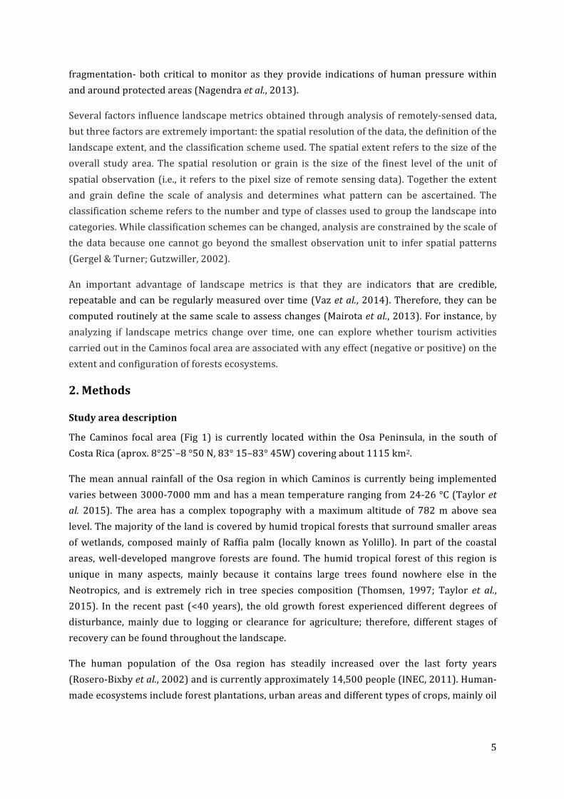
Severalenvironmentalmanagementcategoriesarefoundwithinthisareaincluding:anational

park, a forest reserve, indigenous reserves and several private-owned reserves (commonly

referredtoaswildlifereserves)(Fig1).Eachofthesecategorieshas,bylaw,differentdegreesof

restrictions on the use of its natural resources that can potentially influence its conservation

state.

The Caminos focal area is divided into three main zones, focusing in particular on five

communities located within these zones: Puerto Jimenez, La Palma, El Progreso, Rancho

Quemado,PuertoJimenez,andAgujitas/Drake.Figure2outlinestheboundariesfor3ofthese

communities.3

Figure1ManagementcategorieswithintheCaminosfocalarea.

3 The boundaries of these 3 communities were assessed via a participatory community engagementprocessastheirbordershelpeddeterminethefarthestnorthernextensionoftheCaminosfocalarea.

7

Figure2Outlineof3ofthe5communitiestargetedwithintheCaminosfocalarea(boundariesdeterminedbyparticipatorymapping)

Datasetsdescription

Twotypesofdatawithdifferentspatialresolutionwereusedinthisstudy. Thefirst isatime

series of images fromLandsat satellites,with a spatial resolution of 30m (60m for L2).We

obtained images for 3 dates that span a total of 40 years (Table 1). For each date, onemain

imagewas used (the onewith the best quality and lowest cloud cover over the study area);

anotherimage,separatedby+oneyearfromthismainimage,wasusedtofillinthepartswith

cloudcover.TheLandsatdataweredownloadedfromtheUSGeologicalSurveyviatheGLOVIS

dataportal(glovis.usgs.gov).

Table1Satellitedatausedinthestudy(LandsatScenePath54Row14)

Year Day Landsat sensor Image Quality§ Cloud % § 1975 79* L2 High 3 1979 22** L2 Moderate 0 1999 66** L5 High 0.4 2000 45* L7 High 1.1 2013 280** L8 High 13.6†

2014 043* L8 High 45.9† *Main image of each pair ** Image to fill cloud gaps § as described in the image metadata, cloud cover estimation for the lower left corner of the study area, except for years marked with † where cloud cover estimation is for the whole area.

8

Thesecondtypeofdata is theINOGOMapas; this isa landcoverclassificationof theCaminos

study area based on RapidEye satellite image data, obtained between February and April of

2012.RapidEyedatahasaspatialresolutionof5m;therefore,itcanproduceamoredetailed

land cover mapping than Landsat. Details on INOGO Mapas 2012 data are described in

http://inogo.stanford.edu/resources/INOGOMapas?language=en. To allow comparison

betweendata sets, the land cover classes from INOGOMapaswere reclassified into the same

classesasusedfortheLandsatclassificationinthisstudy(seedescriptioninthenextsection)..

ThisreclassifieddatasetisreferredtoasREintherestofthisreport.

Remotesensinganalysis

To produce a map for each designated date of the analysis, satellite images had to be (pre)

processed. This makes the data comparable between dates and aids in the information

extractionprocess.Thispre-processing removesanyeffects thatdifferences inenvironmental

conditionsoccurringwhentheimageswheretakenmightproduce.Also,pre-processingassures

that images have geographical accuracy, i.e., that the observations between dates are in the

sameplace.

Landsatdataused intheanalysiswereatmosphericallycorrectedusingFLAASHimplemented

inEnvi4.7(ENVI,2006).The1975and1979sceneswereresampledto30msothatthewhole

imagedata sethad the same spatial resolution.Using the year2000 image as a reference, all

imageswereco-registered toobtainapixel-to-pixelcorrespondencebetweendates,obtaining

anaccuracyoflessthanonepixel(30X30m).Imageswerethensegmentedandcloudsegments

were removed from themain image. To fill the gaps caused by removed areas, imageswere

mosaickedwithanotherscenefromtheclosestdateavailable.Thisprocessallowedforalmost

cloud-freedataforeachdate.

The mosaics for each date were processed to derive a series of variables for use in the

classificationprocessincludingvegetationandtextureindices.Dataalsocamefromthetasseled

captransformationandprincipalcomponentanalysis.4Imageclassificationwasdoneusingthe

randomforestsclassifier.Thecombinationofvariablesusedasinputfortheclassifierhelpsto

separatedifferentlandcovertypesbasede.g.,onhowgreenand/orsmoothanareaappearsin

theimage.ThisanalysiswasdoneusingacombinationofR,Envi4.7andOrfeoToolbox.Atotal

of eight classes were identified for the study area including: forest, non-forests, shrubland,

mangrove,oilpalmplantation,forestplantation,wetlandandwater.Theclassifiedimageswere

usedtoproducealandcoverchangedetectionanalysisbetweenthedifferentdates.

4 The variables included in the classification analysis were: Normalized Vegetation Index (NDVI), Soil Adjusted Vegetation Index (SAVI) and Brightness Index (Bi); two texture indices were calculated using the Near Infrared Band (NIR). Two image transformation techniques were then applied: principal component analysis (PCA) and tesseled cap transformation (TC) (Crist & Cicone, 1984).

9

LandscapeMetricAnalysis

LandscapemetricanalysiswascarriedoutusingtheopensourcesoftwareFragstatV4.2 in its

standaloneversion(McGarigal,K.etal.,2012).Insummary,Fragstats4.2usescategoricalmapsoflandcover(inthiscase,derivedfromtheLandsatandRapidEyesatellitedata)tocalculatea

series of metrics that relate to the spatial configuration of these land cover classes and the

landscapecomposition.Allthemetricswerecalculatedusingan8-cellneighborrule.

Metricswereextracted for thewholeCaminos focal area (landscape level) andat the level of

management categories and communities (sub-landscapes). The following metrics were

includedintheanalysis:

• Classarea • Percentage of thelandscape that iscoveredbyeachclass

• Total edge per class(km)

• Classedge(m/ha) • Numberofpatches • Largestpatchindex(%)• Mean patch size (MN

Patch(m2)• Weighted mean patch

(WNPatch(m2))• Totalcorearea

• Nearestneighbor(m) • Mean gyrate (MNGyrate)

• Weighted mean gyrate(WMgyrate)

The description of each landscape metric included in the analysis is provided in the

supplementary information.Todefinewhatwouldbeconsideredascorearea forapatch, the

size of the edgewasdefined for natural ecosystems. For instance, a 100medgewasdefined

betweenforestandnon-forestareas.(TableS1).

To observe how natural ecosystems (forest,mangrove forest andwetlands) in the area have

changed through time, and how these land cover changes reflect on the landscape metrics,

metricswereestimatedforthreedates(1975,2000,2014).Thesedatesrepresentthreepoints

intimewhenmajortransitionsofforestcoverhavebeenreported:highforestcover(in1975),

highdeforestation(in2000)andforestrecovery(in2014).

Thecurrentstateofnaturalecosystems in thestudyareawasdeterminedusingLandsatdata

andREdatathatdifferintheirspatialresolution.Tocomparehowthespatialresolutionofthe

input data affect the estimation of the landscapemetrics, the latter were estimated at 30m

using Landsat data and then compared to a 30 m version of the RE data (from 5m spatial

resolution). The difference in the distribution and the mean size of the patches obtained

through the twosatellitedatasetswascomparedusingaKolmogorov-Smirnoff (K-S)anda t-

test,respectively.

3.Results

LandcoverandchangeinlandcoverthroughoutfourdecadesintheCaminosfocalarea.

The analysis of Landsat datasets of three different dates spanning 40 years on land cover

revealsadynamiclandscape.About13%oftheforestcover(Table2)waslostduringthe1980's

and1990's;aftertheyear2000,thereisevidenceofsomerecoveryoftheforestcover.Within

10

thisdynamiclandscape,forestshavebeenreplacedbyforestoroilpalmplantationsandareas

ofotheragriculturaluses.However,itcanbeobservedthattheareaclassifiedasnon-foresthas

notexperienced importantchanges inthe last15years.Thismay indicatethat theareasused

for agriculture within the Caminos focal area are well established and that clearance and

recovery in those years has occurred mostly on scrubland areas. Mangrove forest has been

reduced.Intermsofwetlandareas,mostoftheseecosystemtypesarelocateddeepwithinthe

CorcovadoNational Park. Thus, observed changes canbe related towater availability rather

thanconversiontootherlanduses.(Fig4).

Table2Baseline landcoverbyyear in theCaminos focalarea(estimatedbasedondata fromLandsattimeseries)

Year /

LandcoverClass

1975

(ha)

2000

(ha)

2014

(ha)

Forest 97713.7 85065.1 88497.3

Non-Forest 10936.6 12706.5 12210.1

MangroveForest 1272.0 1290.7 1085.6

Water 390.3 515.7 247.3

Wetland 967.3 723.9 693.6

Shrubland 220.9 10678.3 6381.0

ForestPlantation

520.5 1125.4

OilPalmPlantation

1260.3

Total1 111500.8 111500.7 111500.8 1TotalareawasestimatedbyexcludingtheNoDataareaforthethreedates.

11

Figure 3 Land cover change map for the Caminos area between 1975 and 2000

12

Figure4LandcoverchangemapfortheCaminosfocalareabetween2000and2014

Changesinnaturalecosystemsthroughtime

In general, the landscapemetrics analysis showed aprocess of fragmentationbetween1975-

2000andaslightrecoveryinfragmentationbetween2000-2014forthenaturalecosystemsof

theCaminosfocalarea.Thisfragmentationprocessisevidencedbyanincreaseinthenumberof

patchesandareductionintheaveragepatchsizeandcoreareasthroughtime(Fig5a,b&c);as

wellasanincreaseintheedgedensity(Fig6a)anddistancebetweenpatches(Fig6b).

However, thisprocess isnot so clear formangrove forestswhere therewasa reduction from2000-2014 in the distance between patches and in the edge density, possibly indicating thatmangrovepatches located towards theouterpartof themangrove forestswere theones thatwerelost.Thetrendin landscapemetricsforwetlandforestsshowsadifferentpatternthat isprobablyrelatedwithseasonaleffects.Thedistributionoftheforestspatches(Fig7)supportsthevaluesobtainedforthelandscapemetrics,showingthattherewasanincreaseintheamountofpatches,reachingapeakin2000followedbyarecoveryofforestcover-seenasareductionin smaller patches and the appearance of patches with bigger areas in 2014.

13

a)

b)

c)

Figure5Mainlandscapemetricstodescribepatchdynamicsofthenaturalecosystemswithin

theCaminosfocalareathroughtime

14

a) b)

c)

Figure6MainlandscapemetricstodescribefragmentationofthenaturalecosystemswithintheCaminosfocalareathroughtime

15

Figure7PatchareadistributionfortheforestclassthroughtimefortheCaminosfocalarea (Patcharearangeconsidered5-300ha)

Comparisonofcurrentstateusinglandscapemetricsatmediumandhighresolution

AfterrecodingthelandcoverclassesfromtheINOGOMapas2012databaseintotheclassesthat

wereusedfortheLandsatdataclassification,theareaforeachlandcoverclasswasestimated

(Table 3). Themost important difference between the two datasets in terms of class area is

foundinthenon-forestclass.Thehigherspatialresolutionmaybecapturingsmallerareas(e.g.

smallclearings)ofnon-forests, therebyincreasingthedetectionofnon-forestsareas.At lower

resolution,thesesmallareaswillbepartofmixedpixelsthatmayalsopresentasforestcover

andthereforebeclassifiedasforest.

*

16

Figure8showstheeffectofthespatialresolutionontheestimationofthelandscapemetricsforthenaturalecosystemsof theCaminos focalarea.Althoughthevaluesof themetricsobtainedwithRapidEyeandLandsatarenotdirectlycomparable,mainlybecausetheclassificationwasderived from two different types of analysis, using data with different spectral and spatialcharacteristics and images from different dates, some general trends can be observed. Ingeneral,Landsatdatapresentalowernumberofpatchesandhighermeanpatchsizeindicating,asmentionedbefore,thatmanysmallareasofnon-forestsorotherlandcovertypesarepartofmixedpixelsandthereforeareobservedasthesamepatch.ThehigherresolutionofRapidEyeisable to separate these small areas of other land covers; hence, more patches are detected.IndeedRapidEyedatadetectsalmostthreetimesmorepatchesthanLandsat(TableS3).

Table3Comparisonbetweenlandcoverclasses(ha)estimatedusingRapidEyeversusLandsat8satellitedata

LandcoverClass

RE_2012

(ha)

L8_2014

(ha)

Absolute

difference1

%ofthetotal

landscapearea2

Forest 89573.7 90687.4 1113.6 0.97

Non-Forest 16744.4 12859.4 3885.0 3.39

MangroveForest 1307.9 1101.6 206.3 0.18

Water 414.5 268.4 146.0 0.13

Wetland 548.7 693.6 144.9 0.13

Scrubland 3502.0 6539.4 3037.4 2.65

ForestPlantation 1231.7 1165.2 66.4 0.06

OilPalmPlantation 1290.7 1298.5 7.9 0.01

Total 114613.5 114613.5 1001 Absolute difference between the land cover estimates 2 Percentage of the total area analyzed that

representsthedifferencebetweenthetwosatellitedatatype

17

a) b)

c)

d)

Figure8LandscapesmetricsforCaminosfocalareaderivedfrommapsproducedfromtwodifferentsensors:Landsat8(2014)andRapidEye(2012)andtheresampleto30mofRapidEyedata

[RapidEye informationwasbasedon INOGOMapas2012a)Numberofpatches,b)Meanpatchsizec)Meancorearea,d)Distancetothenearestpatche)Radiusofgyration,andf)Edgedensity]

18

When the average value is estimated proportionally to the area covered by each patch

(weighted mean patch size), the mean patch area is around 85 000 ha; and, the difference

between sensors is only about 2 500 ha (Table S3). However, this difference becomes larger

whenthetotalcoreareaisconsidered,withLandsatreportingatotalcoreareaofabout82200

ha and RapidEye of 73 700 ha (Table S3). Interpreting these two metrics together, a more

compactblocksofforestareobtainedwiththeLandsatdata;RapidEye,ontheotherhand,hasa

higherspatialdetailof this forestblock thathasavarietyofshapeswhichareaffectedby the

edge.Therefore,thetotalcoreareavalueisdrasticallyreduced.

Interestingly, high resolution (shown in green in Fig 8) and lower resolution RapidEye data

(RapidEyedataresampledto30mtoresembledLandsatresolution,showninpurple)present

verysimilarvaluesindicatingthatlowerresolutiondatadocapturethepatterns,inaconsistent

way.This issupportedby the fact thatnodifferencebetweenthemeanpatchsize for forests,

mangrovesandwetlandswerefound,althoughclearlytheaveragepatchsizewaslargerwhen

calculatedusingLandsatdata(Table4).Similarly,thedistributionofthepatchareasshowsno

significant differences in any of the natural ecosystems (Table 4), indicating that at both

resolutions,asimilarpatternofpatchdistributionisbeingobtained.

Table4Comparisonbetween thedistributionandmeanpatchsize (ha) forLandsat8 (2014)andRE(2012)datasets

Type MeanL8(+sd) MeanRE(+sd) t-test, K-SForest 241.4(4535.5) 159.1(3629.8) W=106787,p=0.78 D=0.09,p=0.02Mangrove 18.9(52.9) 16.99(46.11) t=0.22,p=0.82 D=0.16,p=0.39Wetland 99.0(187.56) 137.02(271.89) t=-.024,p=0.81 D=0.61,p=0.21

e) f)

Figure8(cont’d)

19

4.DiscussionandConclusions

Discussion

The landscapemetricsof theCaminosfocalareaaredominatedbyamainpatchof forestthat

extends from the Parque Nacional Corcovado and continues into the Reserva Forestal Golfo

Dulce.TheCorcovadoNationalParkacts as themain coreareawitha seriesofother smaller

coreareaswithin the reserve.As theareahas recovered forests in thenorthboundaryof the

park, this recovery has contributed to increasing the size of this main patch. Still, the

fragmentationwithintheforestsofGolfoDulceForestReserveisconsiderablyhigher,asshown

byfivetimeshigheredgevaluesobtainedfortheReservethanforCorcovado.

Eventhoughathigherresolutionsmorepatchesaredetected,asexpectedwhenspatialdetailis

increased, the fact thatnosignificantdifferenceswereobservedbetween theaverageand the

distributionofpatchsizeindicatesthatspatialpatternisconsistentatlowandhighresolutions.Itis possible that if there is an increase in fragmentation, the effect of the resolution becomes

moreimportant,asthefrequencyofmediumandsmallpatcheswillincrease.Atthecommunity

level,where there ismore fragmentation, the effect of the resolution ismore significant. For

instance, an extreme case was observed for Rancho Quemado, where Landsat detected 13

patches,whilewithRapidEye,91patcheswereestimated.Thisdifferenceinnumberofpatches

isrelatedtothepresenceofsmallpatches(<2ha),sincethelargestpatchindex(theamountof

areaoccupiedbythelargestpatch)issimilarinbothcasesandismorethan80%.

It is well known that the results of landscapes metrics are highly dependent on the scale

(Forman1995).However,itmustbeclarifiedthatthisdoesn’tmeanthatoneestimateiscorrect

andtheotheriswrong;itjustrevealsthatthesensitivityisdifferent.Indeed,thesedifferences

insensitivityimplythatthecomparisonofa landscapeatdifferentspatialresolutionmightbe

invalid, since the observed differences are due to scale-dependent factors (Gergel & Turner

2002). Moreover, not all landscapes metrics respond similarly or in the same proportion to

changes in spatial resolution. Spatial resolution is particularly important for patch size and

numberandmeasuresthatdependonthem(Gutzwiller,2002).

This dependency of landscape metrics on the spatial resolution has implications for the

developmentofbaselinesandmonitoringefforts.Althoughhavingmoredetail isdesirable, to

establishtrendsandchangesinlandscapespatialpatterns,consistencymightbemoreimportantthanspatialresolution.AsLandsatdataarefreelyavailableandwillcontinuetoprovidedataforthenext25years(Skidomore&Pettorelli,2015;Turneretal.,2015),itisrecommendedtousethemasthebasisformonitoring,astheyhavebeenusedinseveralmonitoringprograms.The

availabilityofaLandsatarchivewillallowonetostudyanypossibleimpactonlandcoverdueto

tourismbefore,duringandafteranyperiodofpotentialconcern.MonitoringwithLandsatcan

be performed on a yearly or evenmonthly basis. Moreover, Landsat monitoring will greatly

20

benefit from the recently launched Sentinal 2A satellite that has a 10 m spatial resolution,

collectscomparabledatatoLandsatandisalsofreelyavailable.Regardless,ifhigherresolution

isavailable, it cancomplement theanalysis;however,Landsatdatawillallow forcomparisonsoveralongertimeperiod.

In terms of the analysis at the community level, the land cover change analysis showed a

dynamic landscape. The three communities of the Caminos focal area considered here have

experienced important deforestation processes between 1975-2000, particularly Rancho

Quemado and El Progreso. However, they have also recovered a significant amount of forest

between 2000-2014. Forest cover gain is especially evident in the southern part of Agujitas.

The estimated land cover at the community level, at both spatial resolutions, is similar; for

example,Landsatestimatesofforestsareonly3%higherthanRapidEye.Nonetheless,RapidEye

datadetectahighernumberofpatches that,not surprisingly, indicates thathigher resolution

data have a higher sensitivity to fragmentation. Each community has different landscape

elements,althoughallofthemaredominatedbyforests.InthecaseofAgujitasandElProgreso,

mangroveareasareclearlyaprioritytomonitorwhileforRanchoQuemadoandElProgreso,oil

palm plantations are important. For instance, as stated previously, although Landsat and

RapidEyearenotdirectlycomparable,inthetwo-yeartemporaldifferenceofthisdata,about30

ha of oil palm are reported in El Progreso. This is evidence of the dynamism that can

characterizetheserurallandscapes.

Finally,therearemoreoptionsthatcouldbeexploredtoestablishmoreaccuratelytheextentof

the resources at the community level; for example, the use of very high-resolution data from

GoogleEarthatthelocallevel.Therearesomerestrictionsonsuchtypeofanalysisbuthasthe

potentialtocomplementthelandscapemetricanalysisandprovideinsights,withhigherdetail,

intotheuseofresourcesincommunitiesatnocostforthedata.

Overall,akeyquestiontoaskishowusefularelandscapemetricstoevaluatetheeffectsofeco-

tourism? Since Caminos implementation is relatively new, it is not possible to analyze how

sensitive the metrics will be to the activities that Caminos is and will be implementing.

However,analyses through timeof the landscapemetricsreveal that theyaresensitive to the

changingculturalandeconomiccircumstancesintheregionthat,inturn,relatestochangesin

thelandcoverwithintheCaminosfocalarea.Forexample,itwaspossibletoobservetrendsin

thelandscapemetricsindicatorsatalowperiodofdeforestation,ahighdeforestationrateanda

recoveryphase.Thisprovidessomedegreeofconfidencethatthesemetricswillbesensitiveto

changesassociatedwithlandcoverrelatedwithecotourismactivity.

Conclusions

Themulti-dateanalysisofLandsatdatashowedthatfortheCaminosfocalareaitisfeasibleto

monitorchangesusing thissetof landscapemetrics throughtime.This isnotsurprisingsince

landscapemetricscomplywithmostofthecriteriadefinedtomonitorsustainabletourism.This

is because they: are critical to ecosystem functions; are responsive to issues that could be

causing stresses to the system; andare identifiable andmeasurable; inotherwords, theyare

21

conceptuallywell founded (Miller & Twining-Ward, 2005). However, thesemetrics require a

highleveloftechnicalskillstoanalyzeandmostlandscapemetricsarenoteasytointerpret.In

thatsensetheyarenot"user-friendly"buttheyareeffectiveand,,contrarytomanyindicators,

arefeasibletomeasure.

Thedifferences inscaleandclassificationmethodsdonotallowone todirectlycompareboth

data sets.Nonetheless, comparisonby increasing the resolutionof theRapidEyedata showed

thatpatternsareconservedbetweenresolutions;however,higherspatialresolutionresultsina

higher detection of smaller patches and non-forests areas. The magnitude of this effect is

differentbetweenecosystemsandisprobablyrelatedtothedegreeoffragmentation.

Outlook

The complex question of what to monitor needs to be critically examined by the multiple

stakeholdersthatareinvolvedinthesustainabletourismorecotourismactivityinaregion.Itis

necessary to understand the effects or impacts that an activitywill have. This is to a certain

point unpredictable but, at a later stage, a program such as Caminos should analyze

comprehensively thepressuresand theeffectson theenvironment that the initiativehashad

andcouldhave.

There are several levels of monitoring tourism effects on biodiversity conservation, ranging

from qualitative/descriptive approaches in which effects are usually estimated through

interviews, to more quantitative evaluations, where information is usually gathered and

analysedthroughecologicalmethods(e.g.throughlandscapemetricsandbiodiversitysurveys).

These two approaches are complementary and, ideally, need to be integrated into a carefully

designed monitoring framework. If the remote sensing-derived indicators presented in this

reportareincorporatedwithinamonitoringframeworkthatitconceptualizedconsideringkey

issues to monitor, and pressures and management responses, they could serve to inform

managementactions.Ideally,amonitoringprogramshouldbeinformedandplannedincluding

differenttypesofstakeholdersthatwillprovidefeedbackontheindicatorstobeusedandthe

baseline.Planningwithdifferentstakeholdersisalsocriticaltounderstandinghowtodefinethe

limitsofacceptablechange.Inthefuture,ifCaminosmonitoringeffortscontinue,theywillneed

toaddressthequestionofwhatwouldbeconsideredasignificantchangeinlandscapemetricsorotherindicatorsthatrequiresaninterventionor,ifanychangecanbeassociatedwithcertaintytoecotourismactivities.

Finally, there are important gaps in how to develop monitoring frameworks for sustainable

tourism;thesegapsareevenstrongerintermsofmonitoringpotentialimpactsonbiodiversity.

Remotesensing-derived indicatorscancontribute todecreasingsuch informationgapsbut, in

order for spatial pattern analysis to reach a full/higher potential and provide valuable

information, it should be carried out within a well- developed monitoring system of the

ecotourismactivity.

22

SupplementaryInformation

S.1Descriptionofthelandscapemetrics

Number of patches: is the basic data required to describe the landscape composition. Twoadjacentgridcells(pixels)ofthesameclassareconsideredtobeinthesamepatchiftheyshare

one border (called the four-neighbor rule) or if they are adjacent or diagonal to each other

(calledtheeight-neighborrule).Inthisanalysis,patchesweredefinedusingtheeight-neighbor

rule.

MeanPatchSize:isthearithmeticaveragesizeofeachpatchwithinagivenclass.Units:ha,m2or

km2.

PatchDensity: equals thenumberofpatchesof thecorrespondingpatch type (NP)dividedbytotallandscapearea.Units:number/100ha

TotalEdge: sumof theedgesperclassor in thewhole landscape.Anedgehappenswhentwoadjacent cellsof thedifferent classes sharea side (nota corner). Inotherwords, it isdefined

usingthefour-neighborrule.

Edge Density: is the total edge found in the landscape. The total count of edges betweendifferent landcover typesdividedby the landscapeareagives theedgedensit .Units:usually

m/haorkm/km2.

Edge to Area ratio: is the total edge by class computed by the total area of that class. It isparticularly useful information since it is specific for each class area. Units: usuallym/ha or

km/km2

TotalCoreArea:sumoftheareaoftheinteriorofthepatchdefinedbyaspecifiededgebufferwidth(definedbytheuserforeachclassorforthewholelandscape).Coreareaisdetermined

bydefiningadistancetothepatchperimeterthatwillbeconsideredanedge.Forexample, in

thisanalysisanedgedepthof100metersbetweenforestsandnon-forestsclasseswasusedto

define the core areas. Core area-relatedmetrics areparticularly important forhabitat-related

analysis.Units:ha

CoreAreaDensity:equalsthetotalnumberofcoreareasofapatchtypedividedbythetotalareaofthatpatchtype.Units:number/100ha

According to MacGarigal et al. 2012 "core area integrates patch size, shape, and edge effect

distanceintoasinglemeasure.Allotherthingsbeingequal,smallerpatcheswithgreatershape

complexityhavelesscorearea."Therefore,coreareaisaveryimportantmeasure.

NearestNeighbor:averagedistancebetweenpatchesofthesametype,measuredasthenearestedge-edgedistancebetweenpatchesofthesameclass.Units:m

23

Gyration:isameasurethatcharacterizesthepatchspatialextent.Patchescanhavesimilarareasbuthaveverydifferentshapesthatinfluencetheirenvironmentalconditions.Itisameasureof

how far a patch extends across a landscape. It can be defined as the average distance one

organism canmovewithin a patchwithout encountering a border from any random starting

point.

Note:standarddeviation(SD)andcoefficientofvariation(CV)areusuallyreportedforsomeof

these metrics and are considered separate metrics. Both SD and CV quantify the variation

among patches in terms of their size, core area, edge, nearest-neighbor distance and spatial

extent(gyration).

TableS1Edgematrix(m)forthelandcoverclassesusedintheanalysis

Classes Forest

Non

Forest Mangrove Water Wetland Shrubland

Forest

Plantation

Oil Palm

Plantation

Forest 0 100 0 0 0 25 50 50

NonForest 0 0 0 0 0 0 0 0

Mangrove 0 200 0 0 0 25 50 50

Water 0 0 0 0 0 0 0 0

Wetland 0 100 0 0 0 25 50 50

Shrubland 0 0 0 0 0 0 0 0

Forest

Plantation 0 0 0 0 0 0 0 0

Oil Palm

Plantation 0 0 0 0 0 0 0 0

24

TableS2LandscapemetricsfortheCaminosfocalarea

Year ClassArea(ha) %

NumberPatches

LargestPatchIndex(%)

TotalEdge(km)

Class-Edge(m/ha)

MN1Patch

(m2)

WMPatch(m2)

SD3Patch

TotalCoreArea(ha)

MN1

NearestNeighbor(m)

MN1_Gyrate(m)

WM2_Gyrate(m)

SD3Gyrate

2014 Forest 88497.3 79.4 527 74.4 2853.9 32.2 168.4 81975.6 3712.0 80968.1 111.6 108.2 13023.0 599.9

2014 NonForest 12210.1 11.0 941 2.2 1867.1 152.9 13.0 1270.3 128.0 12265.2 156.3 87.5 1778.0 190.7

2014 Shrubland 6381.0 5.7 1741 0.7 1984.1 310.9 3.6 134.1 21.8 6350.6 165.8 67.5 438.7 77.3

2014

Oil Palm

Plantation 1260.3 1.1 96 0.1 186.8 148.2 13.2 62.8 25.6 1267.1 339.8 124.2 332.8 115.5

2014

Forest

Plantation 1125.4 1.0 295 0.1 312.8 278.0 3.8 26.4 9.3 1125.8 245.3 72.9 220.8 65.8

2014 Mangrove 1085.6 1.0 68 0.2 124.7 114.8 16.1 162.7 48.6 978.2 242.6 125.7 685.7 201.4

2014 Wetland 693.6 0.6 7 0.4 80.0 115.3 99.1 403.5 173.7 674.3 188.0 376.4 1119.8 428.7

2014 Water 247.3 0.2 116 0.0 57.5 232.6 2.2 7.1 3.3 255.5 351.8 80.0 202.9 89.0

2000 Forest 85065.1 76.3 581 71.3 2935.7 34.5 145.9 78943.4 3390.8 77202.6 128.7 106.3 12873.4 557.1

2000 NonForest 12706.5 11.4 1239 3.5 2324.2 182.9 10.2 1991.9 142.3 12652.2 205.6 81.8 2628.7 197.6

2000 Shrubland 10678.3 9.5 2026 0.4 3236.0 303.0 5.2 81.7 20.0 10602.1 148.9 85.4 381.3 92.8

2000 Mangrove 1290.7 1.2 85 0.3 142.2 110.2 15.2 180.4 50.1 1048.7 872.8 133.0 752.6 208.4

2000 Wetland 723.9 0.6 41 0.6 96.4 133.2 17.7 592.6 100.8 656.3 665.4 90.2 1429.3 237.8

2000

Forest

Plantation 520.5 0.5 146 0.1 144.6 277.7 3.5 24.4 8.6 514.4 671.5 67.8 204.4 61.4

2000 Water 519.7 0.5 105 0.0 84.8 163.1 5.2 16.0 7.5 549.9 351.8 147.5 388.4 174.0

25

1MN=mean2WM=weightedmean3SD=standarddeviationofthemean

TableS3LandscapemetricsofnaturalecosystemsfortheCaminosfocalareabasedondifferentspatialresolutiondata

Year Sensor Class

Area

(ha) %

Number

Patches

Largest

Patch

Index

(%)

Total

Edge

(km)

Class-

Edge

(m/ha)

MN

Patch

(m2)

WM

Patch

(m2)

SD

MN

Patch

Total

Core

Area

(ha)

MN_

Nearest

Neighbor

(m)

MN_

Gyrate

(m)

SD_

MN_

Gyrate

2014 Landsat8 Mangrove 1101.6 1.0 83.0 0.2 132.0 119.9 13.3 163.8 44.7 982.6 247.9 107.0 186.7

2014 Landsat8 Forest 90687.4 79.2 524.0 76.7 3063.7 33.8 173.3 85191.9 3838.4 82207.4 109.7 103.0 611.2

2014 Landsat8 Wetland 693.6 0.6 7.0 0.4 80.4 115.9 99.1 403.5 173.7 674.3 188.0 376.4 428.7

2012 RapidEye Mangrove 1307.9 1.1 186.0 0.2 352.0 269.1 7.0 138.7 30.4 738.9 119.2 76.1 144.3

2012 RapidEye Forest 89573.7 78.2 1622.0 75.1 5060.1 56.5 55.2 82680.0 2136.1 73688.2 35.8 52.2 344.9

2012 RapidEye Wetland 548.7 0.5 9.0 0.5 87.5 159.5 61.0 541.0 171.1 485.8 14.6 177.2 412.1

2012 RE_30 Mangrove 1310.3 1.1 173.0 0.2 252.7 192.9 7.6 140.7 31.8 746.7 150.0 76.1 145.6

2012 RE_30 Forest 89577.9 78.1 1312.0 75.5 3654.9 R 68.3 83641.3 2388.7 76564.4 80.4 56.0 383.3

2012 RE_30 Wetland 547.6 0.5 15.0 0.5 54.9 100.3 36.5 538.2 135.3 498.1 62.4 112.4 328.91MN=mean2WM=weightedmean3SD=standarddeviationofthemean

1975 Forest 97713.7 87.6 129 83.7 867.7 8.9 757.8 94319.0 8420.2 92458.8 142.7 214.4 13358.6 1193.5

1975 NonForest 10936.6 9.8 249 3.8 774.7 70.8 44.0 2182.1 306.6 10944.2 371.8 186.2 2692.6 380.1

1975 Mangrove 1272.0 1.1 51 0.3 96.5 75.8 25.2 172.7 61.0 1075.5 255.7 181.5 636.9 203.9

1975 Wetland 967.3 0.9 16 0.8 106.4 110.0 60.4 800.7 211.4 739.1 1165.3 167.6 1317.2 332.8

1975 Water 390.3 0.4 75 0.0 42.8 109.8 5.7 14.8 7.2 427.0 561.2 123.2 262.9 118.6

1975 Shrubland 220.9 0.2 23 0.1 41.7 188.9 9.6 29.0 13.6 220.1 1106.6 128.0 254.7 94.3

26

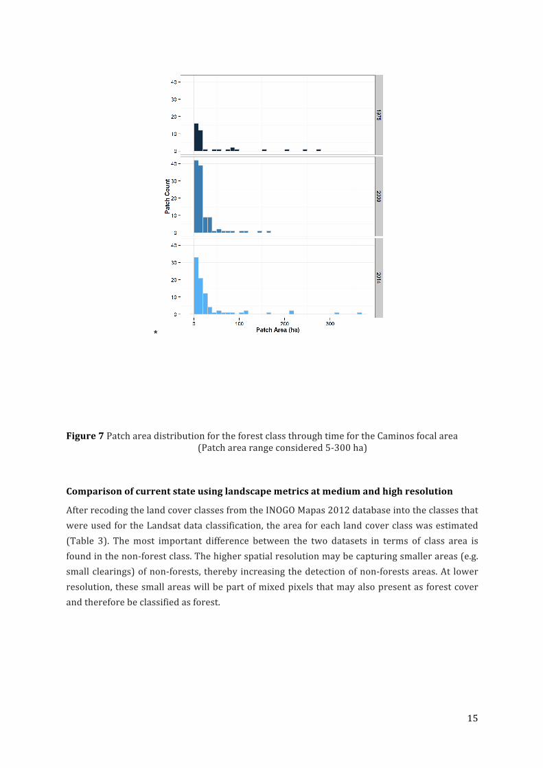
TableS4LandscapemetricsbymanagementcategoriesaccordingtoLandsat8for2014andRapidEye2012

Category Class

Area

(ha) %

Number

of

Patches

Largest

Patch

Index

(%)

Total

Edge

(km)

Class

Edge

(m/ha)

MN

Patch

(m2)

WM

Patch

(m2) SDPatch

Total

Core

Area

(ha)

MN

Nearest

Neighbor

(m)

MN

Gyrate

(m)

WM

Gyrate

(m)

SD

Gyrate

Landsat8

HH Forest 20.0 67.5 5 34.7 2.07 103.6 4.0 8.4 4.2 10.8 140.9 104.9 199.0 90.7

HH NonForest 5.4 18.2 5 10.6 1.74 322.2 1.1 2.2 1.1 5.4 106.2 40.6 62.3 23.2

HH Shrubland 3.5 11.9 4 4.3 1.29 367.5 0.9 1.1 0.4 3.5 437.2 43.8 52.9 19.4

HH Water 0.7 2.4 4 0.9 0.51 708.3 0.2 0.2 0.1 0.7 143.5 17.3 18.5 2.3

RF Forest 32865.2 87.0 116 44.0 1187.79 36.1 283.3 16112.9 2117.7 29697.7 86.7 173.8 6930.3 911.0

RF NonForest 1961.7 5.2 461 0.8 520.83 265.5 4.3 88.8 19.0 1961.7 181.5 67.9 400.7 85.1

RF Shrubland 2524.3 6.7 813 0.5 836.46 331.4 3.1 48.2 11.8 2524.3 166.6 64.1 308.8 72.7

RF

Oil Palm

Plantation 79.8 0.2 14 0.1 18.09 226.6 5.7 16.5 7.9 79.8 1122.1 92.0 172.3 60.8

RF

Forest

Plantation 355.7 0.9 145 0.1 124.92 351.2 2.5 11.2 4.6 355.7 299.0 60.5 136.5 44.2

RF Mangrove 1.8 0.0 3 0.0 1.11 616.7 0.6 0.8 0.3 0.9 544.7 32.0 38.5 13.0

RF Water 7.9 0.0 4 0.0 1.86 234.8 2.0 2.6 1.1 7.9 2317.0 63.3 80.6 30.1

PN Forest 40686.0 95.9 33 95.8 298.44 7.3 1232.9 40643.7 6970.7 40217.1 98.9 300.4 8863.9 1514.7

PN NonForest 298.4 0.7 133 0.1 92.37 309.6 2.2 15.3 5.4 298.4 290.3 64.2 238.1 83.6

PN Shrubland 594.3 1.4 201 0.4 196.47 330.6 3.0 60.2 13.0 594.3 371.7 66.0 337.1 71.5

27

PN

Forest

Plantation 4.5 0.0 4 0.0 2.28 506.7 1.1 1.5 0.6 4.5 3648.2 46.3 53.9 15.3

PN Mangrove 115.7 0.3 9 0.2 22.41 193.6 12.9 44.2 20.1 108.5 231.1 174.7 510.4 217.0

PN Water 41.9 0.1 30 0.0 13.38 319.7 1.4 10.3 3.5 41.9 318.1 44.9 233.2 74.6

RVS Forest 2278.7 74.5 80 39.8 89.4 39.2 28.5 716.8 140.0 2194.2 167.5 115.7 957.4 200.2

RVS NonForest 258.4 8.4 50 3.9 37.05 143.4 5.2 64.8 17.6 258.4 397.3 76.4 370.0 110.5

RVS Shrubland 445.0 14.5 90 4.8 96.81 217.6 4.9 66.4 17.4 445.0 196.9 70.7 359.4 97.3

RVS Wetland 693.5 1.6 7 1.2 80.4 115.9 99.1 403.5 173.7 674.3 188.0 376.4 1119.8 428.7

RVS Water 8.1 0.3 6 0.1 2.28 281.5 1.4 3.4 1.7 8.1 3336.3 55.4 112.9 48.5

RI Forest 2538.5 93.8 4 93.7 56.64 22.3 634.6 2536.1 1098.5 2341.0 93.6 634.8 2463.6 1056.5

RI NonForest 72.1 2.7 38 0.5 28.62 397.0 1.9 5.0 2.4 72.1 175.6 56.8 107.2 41.1

RI Shrubland 96.8 3.6 56 0.2 43.44 449.0 1.7 2.8 1.3 96.8 194.5 58.3 75.1 23.8

RI Mangrove 68.5 2.2 11 1.9 10.08 147.2 6.2 49.2 16.3 47.9 76.0 70.6 296.9 92.1

RapidEye

HH Forest 12.0 38.4 8 16.2 2.785 231.2 1.5 3.5 1.7 4.4 90.7 51.0 95.1 40.9

HH NonForest 5.9 18.7 13 8.1 5.695 968.5 0.5 1.7 0.8 5.9 67.2 41.2 126.1 53.2

HH Shrubland 3.5 11.3 9 5.6 3.435 969.7 0.4 1.1 0.5 3.5 36.3 31.9 77.1 34.4

HH Water 9.9 31.7 9 27.1 4.01 403.3 1.1 7.4 2.6 9.9 78.6 43.4 245.7 84.9

PN Forest 41033.3 96.7 78 96.6 367.975 9.0 526.1 40977.9 4613.1 39263.1 23.5 136.9 8895.2 999.3

PN NonForest 698.4 1.6 383 0.8 276.565 396.0 1.8 189.8 18.5 698.4 143.1 47.6 543.6 84.6

PN Shrubland 87.9 0.2 71 0.1 50.055 569.2 1.2 12.5 3.7 87.9 487.8 41.9 238.5 67.0

PN Mangrove 30.0 0.1 42 0.0 28.47 949.2 0.7 3.2 1.3 22.2 18.6 33.6 102.9 41.4

PN Wetland 548.7 1.3 9 1.3 87.51 159.5 61.0 541.0 171.1 485.8 14.6 177.2 1331.8 412.1

PN Water 45.1 0.1 72 0.0 36.65 812.8 0.6 2.0 0.9 45.1 353.9 44.9 117.4 53.3

28

RF Forest 32546.3 86.1 580 42.8

1927.26

5 59.2 56.1 15789.2 939.6 25649.9 23.1 51.3 6793.0 405.6

RF NonForest 3516.1 9.3 1221 0.9 1466.93 417.2 2.9 102.0 16.9 3516.1 65.4 45.4 448.4 82.8

RF Shrubland 1459.6 3.9 688 0.4 867.755 594.5 2.1 33.6 8.2 1459.6 114.0 48.3 284.2 70.4

RF

Oil Palm

Plantation 2.9 0.0 14 0.0 3.25 1131.4 0.2 0.9 0.4 2.9 842.6 16.5 56.8 21.6

RF

Forest

Plantation 276.0 0.7 91 0.2 110.435 400.2 3.0 39.7 10.5 276.0 232.1 45.2 305.1 81.2

RF Mangrove 3.8 0.0 12 0.0 4.21 1097.8 0.3 0.7 0.4 2.2 1312.5 26.1 48.7 20.9

RF Water 15.3 0.0 30 0.0 13.145 857.6 0.5 1.5 0.7 15.3 674.4 34.5 63.0 28.1

RI Forest 2514.2 92.9 35 92.6 86.23 34.3 71.8 2495.5 417.3 2234.2 19.7 87.1 2430.2 403.8

RI NonForest 80.0 3.0 71 0.4 49.55 619.5 1.1 5.2 2.1 80.0 106.6 35.2 106.7 40.3

RI Shrubland 111.4 4.1 16 2.0 57.27 514.3 7.0 41.0 15.4 111.4 30.8 79.5 297.5 101.8

RVS Forest 2331.3 76.5 112 40.3 166.58 71.5 20.8 710.3 119.8 1827.9 65.3 95.4 957.2 183.4

RVS NonForest 400.6 13.1 206 6.5 120.825 301.6 1.9 106.6 14.3 400.6 95.7 39.6 439.9 71.6

RVS Shrubland 221.5 7.3 123 1.6 118.945 537.0 1.8 23.7 6.3 221.5 118.7 42.0 259.4 66.7

RVS Mangrove 67.7 2.2 11 1.8 15.24 225.2 6.2 46.7 15.8 14.2 28.9 80.7 295.6 100.7

RVS Water 25.3 0.8 9 0.5 7.015 277.8 2.8 9.0 4.2 25.3 2497.5 98.9 296.0 133.81MN=mean2WM=weightedmean3SD=standarddeviationofthemean

29

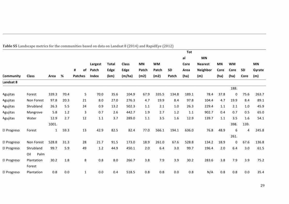
TableS5LandscapemetricsforthecommunitiesbasedondataonLandsat8(2014)andRapidEye(2012)

Community Class Area %

# of

Patches

Largest

Patch

Index

Total

Edge

(km)

Class

Edge

(m/ha)

MN

Patch

(m2)

WM

Patch

(m2)

SD

Patch

Tot

al

Core

Area

(ha)

MN

Nearest

Neighbor

(m)

MN

Core

(ha)

WM

Core

(ha)

SD

Core

MN

Gyrate

(m)

Landsat8

Agujitas Forest 339.3 70.4 5 70.0 35.6 104.9 67.9 335.5 134.8 189.1 78.4 37.8

188.

0 75.6 263.7

Agujitas NonForest 97.8 20.3 21 8.0 27.0 276.3 4.7 19.9 8.4 97.8 104.4 4.7 19.9 8.4 89.1

Agujitas Shrubland 26.3 5.5 24 0.9 13.2 502.3 1.1 2.1 1.0 26.3 229.4 1.1 2.1 1.0 45.9

Agujitas Mangrove 5.8 1.2 3 0.7 2.6 442.7 1.9 2.7 1.2 1.1 902.7 0.4 0.7 0.5 65.0

Agujitas Water 12.9 2.7 12 1.1 3.7 289.0 1.1 3.5 1.6 12.9 139.7 1.1 3.5 1.6 54.1

ElProgreso Forest

1001.

1 59.3 13 42.9 82.5 82.4 77.0 566.1 194.1 636.0 76.8 48.9

398.

6

139.

4 245.8

ElProgreso NonForest 528.8 31.3 28 21.7 91.5 173.0 18.9 261.0 67.6 528.8 134.2 18.9

261.

0 67.6 136.8

ElProgreso Shrubland 99.7 5.9 49 1.2 44.9 450.1 2.0 6.4 3.0 99.7 196.4 2.0 6.4 3.0 61.5

ElProgreso

Oil Palm

Plantation 30.2 1.8 8 0.8 8.0 266.7 3.8 7.9 3.9 30.2 283.6 3.8 7.9 3.9 75.2

ElProgreso

Forest

Plantation 0.8 0.0 1 0.0 0.4 518.5 0.8 0.8 0.0 0.8 N/A 0.8 0.8 0.0 35.4

30

ElProgreso Mangrove 6.1 0.4 7 0.1 3.9 642.2 0.9 1.3 0.6 0.9 414.0 0.1 0.1 0.3 45.4

ElProgreso Water 22.4 1.3 9 0.3 5.6 251.7 2.5 3.3 1.5 22.4 89.8 2.5 3.3 1.5 116.8

Rancho

Quemado Forest

5333.

0 86.5 13 85.2 135.0 25.3 410.2 5170.9 1397.5 4905.3 87.8

377.

3

4808

.2

1300

.7 338.3

Rancho

Quemado NonForest 421.1 6.8 27 4.8 78.7 186.9 15.6 217.6 56.1 421.1 358.2 15.6

217.

6 56.1 113.6

Rancho

Quemado Shrubland 213.5 3.5 101 0.3 89.0 416.8 2.1 5.2 2.5 213.5 230.4 2.1 5.2 2.5 62.4

Rancho

Quemado

Oil Palm

Plantation 29.0 0.5 3 0.4 5.0 171.8 9.7 23.2 11.5 29.0 400.0 9.7 23.2 11.5 105.4

Rancho

Quemado

Forest

Plantation 163.3 2.6 22 0.5 34.1 209.1 7.4 20.1 9.7 163.3 217.9 7.4 20.1 9.7 98.4

Rancho

Quemado Water 2.1 0.0 1 0.0 0.7 318.8 2.1 2.1 0.0 2.1 N/A 2.1 2.1 0.0 60.9

RapidEye

Agujitas Forest 327.8 67.9 27 38.3 52.1 158.8 12.1 160.7 42.5 118.6 25.0 4.4 59.4 15.7 72.8

Agujitas NonForest 114.8 23.8 49 7.6 52.4 456.6 2.3 20.5 6.5 114.8 41.5 2.3 20.5 6.5 53.9

Agujitas Shrubland 13.5 2.8 12 0.9 12.1 897.1 1.1 2.5 1.2 13.5 149.0 1.1 2.5 1.2 62.4

Agujitas Mangrove 12.0 2.5 3 2.1 5.7 474.3 4.0 8.5 4.3 0.0 17.2 0.0 0.0 0.0 123.8

Agujitas Water 15.0 3.1 19 1.4 9.0 600.0 0.8 3.7 1.5 15.0 48.2 0.8 3.7 1.5 47.7

ElProgreso Forest 899.6 53.2 31 40.2 121.3 134.8 29.0 540.9 121.9 453.9 66.1 14.6

317.

3 72.7 123.5

ElProgreso NonForest 637.1 37.7 65 31.3 141.7 222.4 9.8 442.6 65.1 637.1 48.7 9.8

442.

6 65.1 68.9

31

ElProgreso Shrubland 84.0 5.0 40 1.1 59.2 704.0 2.1 8.4 3.6 84.0 144.1 2.1 8.4 3.6 67.1

ElProgreso

Forest

Plantation 0.5 0.0 2 0.0 0.9 1809.0 0.2 0.3 0.1 0.5 920.4 0.2 0.3 0.1 46.2

ElProgreso Mangrove 31.8 1.9 18 1.1 12.3 386.1 1.8 13.2 4.5 10.3 133.3 0.6 5.5 2.1 42.7

ElProgreso Water 38.1 2.3 16 1.2 19.7 518.1 2.4 13.2 5.1 38.1 116.1 2.4 13.2 5.1 120.1

Rancho

Quemado Forest

5120.

9 83.1 91 81.3 233.4 45.6 56.3 4908.4 522.5 4336.2 25.0 47.7

4239

.0

451.

4 70.1

Rancho

Quemado NonForest 573.8 9.3 130 5.6 186.9 325.6 4.4 215.3 30.5 573.8 78.7 4.4

215.

3 30.5 47.5

Rancho

Quemado Shrubland 203.7 3.3 88 2.3 92.4 453.7 2.3 99.1 15.0 203.7 63.6 2.3 99.1 15.0 40.8

Rancho

Quemado

Oil Palm

Plantation 0.9 0.0 4 0.0 1.1 1229.0 0.2 0.3 0.1 0.9 201.5 0.2 0.3 0.1 19.0

Rancho

Quemado

Forest

Plantation 262.9 4.3 70 1.2 99.5 378.6 3.8 41.5 11.9 262.9 26.3 3.8 41.5 11.9 49.9

Rancho

Quemado Water 3.0 0.0 1 0.0 1.2 381.9 3.0 3.0 0.0 3.0 N/A 3.0 3.0 0.0 71.2

32

References

AlmeidaCunhaA(2010)NegativeeffectsoftourisminaBrazilianAtlanticforestNationalPark.JournalforNatureConservation,18,291–295.

Corbane C, Lang S, Pipkins K et al. (2015) Remote sensing formapping natural habitats andtheir conservation status - New opportunities and challenges. International Journal ofAppliedEarthObservationandGeoinformation,37,7–16.

CristEP,CiconeR.(1984)Aphysically-basedtransformationofThematicMapperdata-theTMTasseledCap.IEEETransactionsonGeoscienceandRemoteSensing,22,256–263.

Fahrig L (2003) Effects of habitat fragmentation on Biodiversity. Annual Review of Ecology,Evolution,andSystematics,34,487–515.

FoleyJA,DefriesR,AsnerGPetal.(2005)Globalconsequencesoflanduse.Science(NewYork,N.Y.),309,570–4.

GergelSE,TurnerMGLearninglandscapeecology:apracticalguidetoconceptsandtechniques.

GutzwillerKJ(2002)Applyinglandscapeecologyinbiologicalconservation.

HorningN,RobinsonJA,SterlingEJ,TurnerW,SpectorS(2010)RemotesensingforEcologyandConservation.

HuntCA,DurhamWH,DriscollL,HoneyM(2014)Canecotourismdeliverrealeconomic,social,and environmental benefits? A study of the Osa Peninsula, Costa Rica. Journal ofSustainableTourism,23,339–357.

INEC(2011)Censogeneraldepoblacion2011. InstitutoNacionaldeEstadisticayCensos.SanJose,CostaRica.

Koens JF,DieperinkC,MirandaM (2009)Ecotourismas adevelopment strategy:ExperiencesfromCostaRica.Environment,DevelopmentandSustainability,11,1225–1237.

KrügerO(2005)Theroleofecotourisminconservation:panaceaorPandora’sbox?Biodiversity&Conservation,14,579–600.

Mairota P, Cafarelli B, Boccaccio L, Leronni V, Labadessa R, Kosmidou V, NagendraH (2013)Usinglandscapestructuretodevelopquantitativebaselinesforprotectedareamonitoring.EcologicalIndicators,33,82–95.

McGarigal,K., CushmanS, EneE (2012)FRAGSTATSv4: Spatial PatternAnalysisProgram forCategoricalandContinuousMaps.Computersoftwareprogramproducedbytheauthorsatthe University of Massachusetts, Amherst. Available at the following web site:http://www.umass.edu/landeco/research/f.

Miller G, Twining-Ward L (2005) Monitoring for a sustainable tourism transition. CABIPublishing,Cambridge,MA,USA,324pp.

MincaC,LindaM(2000)EcotourismontheEdge :theCaseofCorcovado.Recreation,103–126.

Nagendra H, Lucas R, Honrado JP, Jongman RHG, Tarantino C, Adamo M, Mairota P (2013)Remote sensing for conservation monitoring: Assessing protected areas, habitat extent,habitatcondition,speciesdiversity,andthreats.EcologicalIndicators,33,45–59.

Newsome D, Moore SA, Dowling RK (2013) Natural area tourism: ecology, impacts and

33

management.2nd.

Rocchini D, Hernández-stefanoni JL, He KS (2015) Ecological Informatics Advancing speciesdiversity estimate by remotely sensed proxies : A conceptual review. EcologicalInformatics,25,22–28.

Rosero-BixbyL,MaldonadoT,Bonilla-CarriónR(2002)BosqueypoblaciónenlaPenínsuladeOsa,CostaRica.RevistadeBiologíaTropical,50,585–598.

SkidomoreA,PettorelliN(2015)metricsto.Nature,523,5–7.

StemCJ,Lassoie JP,LeeDR,DeshlerDJ (2003)How“Eco” isEcotourism?AComparativeCaseStudyofEcotourisminCostaRica.JournalofSustainableTourism,11,322–347.

StrandH,HöftR, Strittholt J,MilesL,HorningN, FosnightE,TurnerW (2007)Sourcebookonremotesensingandbiodiversityindicators,Technicaledn.SecretariatoftheConventiononBiologicalDiversity,Montreal,Canada,203pp.

Taylor P, Asner G, Dahlin K et al. (2015) Landscape-Scale Controls on Aboveground ForestCarbonStocksontheOsaPeninsula,CostaRica.PloSone,10,e0126748.

ThomsenK(1997)PotentialofnontimberforestproductsinatropicalrainforestsinCostaRica.UniversityofCopenhagen.

TurnerW,RondininiC,PettorelliNetal.(2015)Freeandopen-accesssatellitedataarekeytobiodiversityconservation.BiologicalConservation,182,173–176.

VazAS,MarcosB,GonçalvesJetal.(2014)Canwepredicthabitatqualityfromspace?Amulti-indicator assessment based on an automated knowledge-driven system. InternationalJournalofAppliedEarthObservationandGeoinformation,37,106–113.