IZA DP No. 2265

Phillips Curves and Unemployment Dynamics:A Critique and a Holistic Perspective

Marika KaranassouHector SalaDennis J. Snower

DI

SC

US

SI

ON

PA

PE

R S

ER

IE

S

Forschungsinstitutzur Zukunft der ArbeitInstitute for the Studyof Labor

August 2006

Phillips Curves and

Unemployment Dynamics: A Critique and a Holistic Perspective

Marika Karanassou

Queen Mary, University of London and IZA Bonn

Hector Sala

Universitat Autònoma de Barcelona and IZA Bonn

Dennis J. Snower

Kiel Institute for World Economics, University of Kiel, CEPR and IZA Bonn

Discussion Paper No. 2265 August 2006

IZA

P.O. Box 7240 53072 Bonn

Germany

Phone: +49-228-3894-0 Fax: +49-228-3894-180

Email: iza@iza.org

Any opinions expressed here are those of the author(s) and not those of the institute. Research disseminated by IZA may include views on policy, but the institute itself takes no institutional policy positions. The Institute for the Study of Labor (IZA) in Bonn is a local and virtual international research center and a place of communication between science, politics and business. IZA is an independent nonprofit company supported by Deutsche Post World Net. The center is associated with the University of Bonn and offers a stimulating research environment through its research networks, research support, and visitors and doctoral programs. IZA engages in (i) original and internationally competitive research in all fields of labor economics, (ii) development of policy concepts, and (iii) dissemination of research results and concepts to the interested public. IZA Discussion Papers often represent preliminary work and are circulated to encourage discussion. Citation of such a paper should account for its provisional character. A revised version may be available directly from the author.

IZA Discussion Paper No. 2265 August 2006

ABSTRACT

Phillips Curves and Unemployment Dynamics: A Critique and a Holistic Perspective*

The conventional wisdom that inflation and unemployment are unrelated in the long-run implies that these phenomena can be analysed by separate branches of economics. The macro literature tries to explain inflation dynamics and estimates the NAIRU. The labour macro literature tries to explain unemployment dynamics and determine the real economic factors that drive the natural rate of unemployment. We show that the orthodox view that the New Keynesian Phillips curve is vertical in the long-run and that it cannot generate substantial inflation persistence relies on the implausible assumption of a zero interest rate. In the light of these results, we argue that a holistic framework is needed to jointly explain the evolution of inflation and unemployment. JEL Classification: E24, E31 Keywords: natural rate of unemployment, NAIRU, New Keynesian Phillips Curve,

inflation-unemployment tradeoff, inflation dynamics, unemployment dynamics Corresponding author: Marika Karanassou Department of Economics Queen Mary, University of London Mile End Road London E1 4NS United Kingdom E-mail: M.Karanassou@qmul.ac.uk

* Hector Sala is grateful to the Spanish Ministry of Education for financial support through grant SEC2003-7928.

1 Introduction

In this paper we are concerned with two main categories of dynamic macro models.

Phillips curve (PC) models that aim to explain inflation dynamics and models that seek

to explain the evolution of the unemployment rate. Both types of models are intricately

related with the natural rate of unemployment (NRU) hypothesis. The NRU is a re-

flection of the classical dichotomy, hence it implies that the phenomena of inflation and

unemployment can be analysed by separate models. The macro literature tries to ex-

plain inflation dynamics. The labour macro literature tries to identify the determinants

of the unemployment rate.

We argue that a long-run inflation-unemployment tradeoff exists, and thus we pro-

pose a holistic approach that can both model inflation dynamics and identify the driving

forces of unemployment.

Inflation dynamics models treat the NRU as "exogenous" in the sense that the models

do not identify the factors underlying its changes. Mainstream PC models estimate the

NRU as the unemployment rate compatible with inflation stability - this is commonly

referred to as the non accelerating inflation rate of unemployment (NAIRU) - and focus

on the inflation-unemployment tradeoff.

On the other hand, unemployment rate models endogenise the NRU and determine

the economic factors which influence it. These "endogenous" NRU models can be used

to explain the long-run changes in equilibrium unemployment by identifying the business

cycle and trend components of the model.1

In the context of economic models with frictions (e.g. wage/price staggering, in-

formational stickiness, real rigidities, etc.), it is convenient to distinguish between two

versions of the NRU hypothesis: In the strong-form NRU monetary policy has no effect

on the equilibrium unemployment rate in both the short- and long-run, whereas in the

weak-form NRU monetary changes have temporary (short-run) effects on unemployment

but no long-run effects. In other words, the weak-form NRU states that the equilibrium

unemployment rate is independent of monetary variables only in the long-run.

The conventional wisdom is that the weak-form NRU hypothesis holds in inflation

dynamics models such as the Expectations Augmented Phillips Curve (EAPC) - and

its subsequent developments (triangle model of inflation, TV-NAIRU) - and the New

Keynesian Phillips Curve (NPC)2. The belief in the classical dichotomy implies the

existence of a vertical long-run Phillips curve whose intersection with the horizontal

axis gives the NRU.

1Tobin (1998) argues that the NAIRU and NRU are not synonymous. However, such a distinctionbecomes superfluous within our framework of "exogenous/endogenous" NRU models.

2For the etymology of the term "New Keynesian", see Gordon (1990). It is often also called the“New Phillips curve” or the “New Neoclassical Synthesis.” Helpful surveys include Clarida, Gali andGertler (1999), Gali (2003), Mankiw (2001), Roberts (1995) and Goodfriend and King (1997).

2

Unemployment models analyse the structure of the labour market through tradi-

tional dynamics (i.e. single unemployment rate equations) or interactive dynamics (i.e.

multi-equation systems with spillover effects). There is an important disparity between

the two approaches regarding the NRU hypothesis. It can be shown that in interac-

tive dynamics models, as opposed to single unemployment rate dynamic equations, the

NRU is misleading as a reference point for the long-run movements of the equilibrium

unemployment rate when the exogenous variables have constant but nonzero long-run

growth rates.

Furthermore, recent models of the NPC show that a downward sloping PC does exist

and money is not super-neutral. We call these models the Frictional Growth New Key-

nesian Phillips Curve (FG-NPC) and their contribution is to demonstrate that even the

slightest asymmetry in the backward- and forward-looking elements of price behaviour

can generate a significant long-run tradeoff between real and nominal variables. This

asymmetry arises because of time discounting and a nonzero interest rate. In other

words, whereas the standard NPC is consistent with the weak-form NRU hypothesis,

the FG-NPC refutes it.3

Table 1 summarises the above classification of inflation/unemployment models. As

pointed out, these are commonly considered as separate branches of study.

Table 1: The dichotomy in inflation/unemployment modelsInflation Dynamics Models

(Exogenous NRU)| {z }. &

Old PC| {z } New Keynesian PC| {z }. ↓ ↓ ↓

Traditional EAPC Standard

NPC

Frictional

Growth NPC

Unemployment Theories(Endogenous NRU)| {z }

. &Traditional

Dynamics(single-equation)

Interactive

Dynamics(multi-equation)

From the empirical side, a number of recent papers have also started to question

the dichotomy between the real and nominal sides of the economy, and consider the

possibility of long-lasting effects derived from changes in the monetary policy. For

example, Fisher and Seater (1993), King and Watson (1994) and Fair (2000) find a long-

run inflation-unemployment tradeoff; Campbell andMankiw (1987) find long-lasting real

GDP responses to monetary disturbances in the US; along the same lines, the real GDP

impulse response function (IRF hereafter) estimated by Bernanke andMihov (1998) does

not converge to zero (albeit the standard errors increase enough to include the zero line);

Ball (1997 and 1999) studies the OECD countries and relates long disinflationary periods

with increases in their NRUs; Dolado, López-Salido and Vega (2000) provide scenarios of

3Karanassou and Snower (2004) show that the standard formulation of the NPC is simply a highlyimplausible restricted case of price/wage staggering.

3

nonvertical long-run Phillips curve slopes for Spain; Akerlof, Dickens, and Perry (1996

and 2000) claim that at low inflation levels departures from fully rational decisions

generate inflation-unemployment long-run tradeoffs; more recently, Karanassou, Sala

and Snower (2002, 2003b and 2005) present empirical unemployment IRFs for Spain,

the EU and the US which do not converge to the initial equilibriumwhen these economies

are hit by a permanent monetary shock.

Theoretical and empirical evidence against the classical dichotomy calls for a holistic

approach that takes into account the intimate dynamic relation between inflation and

unemployment.

The structure of the paper is as follows. Section 2 gives the definitions of some

fundamental concepts in dynamic macro models: the short-run, long-run, and steady-

state equilibriums of a stochastic process. Section 3 outlines the standard Phillips curve

models, as they developed over the decades and singles out the restrictions under which

there is no inflation-unemployment tradeoff in the long-run. Section 4 discusses and

compares the traditional and interactive dynamics theories of unemployment. Section

5 presents the theoretical underpinnings of a non-vertical Phillips curve. Section 6 pro-

poses a holistic framework that aims to jointly analyse the inflation and unemployment

phenomena. Finally, Section 7 concludes.

2 Concepts and Definitions

To facilitate our analysis, we first offer clear definitions of the widely used, and occasion-

ally confused, concepts of equilibrium: short-run, steady-state, and long-run. In what

follows the dependent variable yt refers to (the log of) a macroeconomic magnitude, e.g.

unemployment rate, inflation rate, output, marginal costs, etc.

Considering a stochastic equation for the macro variable yt, the short-run (SR) equi-

librium is given by the conditional expectation of yt given the values of the explanatory

variables, while the long-run (LR) equilibrium is the unconditional expectation of the

stochastic process.

We start our exposition with the following static equation:

yt = γxt + εt, (1)

where xt is a k× 1 vector of exogenous variables, γ is a 1× k vector of coefficients, and

εt is a strict white noise error term (i.e. independently, identically distributed with zero

mean and constant variance). It is easy to see that the SR equilibrium of yt is simply

Exyt = γxt, (2)

4

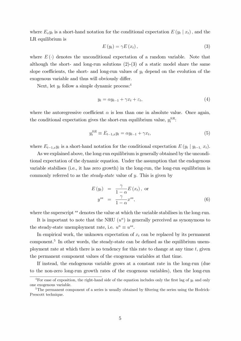
where Exyt is a short-hand notation for the conditional expectation E (yt | xt) , and theLR equilibrium is

E (yt) = γE (xt) , (3)

where E (·) denotes the unconditional expectation of a random variable. Note that

although the short- and long-run solutions (2)-(3) of a static model share the same

slope coefficients, the short- and long-run values of yt depend on the evolution of the

exogenous variable and thus will obviously differ.

Next, let yt follow a simple dynamic process:4

yt = αyt−1 + γxt + εt, (4)

where the autoregressive coefficient α is less than one in absolute value. Once again,

the conditional expectation gives the short-run equilibrium value, ySRt :

ySRt ≡ Et−1,xyt = αyt−1 + γxt, (5)

where Et−1,xyt is a short-hand notation for the conditional expectation E (yt | yt−1, xt).As we explained above, the long-run equilibrium is generally obtained by the uncondi-

tional expectation of the dynamic equation. Under the assumption that the endogenous

variable stabilises (i.e., it has zero growth) in the long-run, the long-run equilibrium is

commonly referred to as the steady-state value of y. This is given by

E (yt) =γ

1− αE (xt) , or

yss =γ

1− αxss, (6)

where the superscript ss denotes the value at which the variable stabilises in the long-run.

It is important to note that the NRU (un) is generally perceived as synonymous to

the steady-state unemployment rate, i.e. un ≡ uss.

In empirical work, the unknown expectation of xt can be replaced by its permanent

component.5 In other words, the steady-state can be defined as the equilibrium unem-

ployment rate at which there is no tendency for this rate to change at any time t, given

the permanent component values of the exogenous variables at that time.

If instead, the endogenous variable grows at a constant rate in the long-run (due

to the non-zero long-run growth rates of the exogenous variables), then the long-run

4For ease of exposition, the right-hand side of the equation includes only the first lag of yt and onlyone exogenous variable.

5The permanent component of a series is usually obtained by filtering the series using the Hodrick-Prescott technique.

5

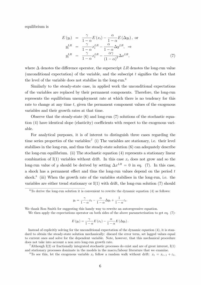
equilibrium is

E (yt) =γ

1− αE (xt)−

α

1− αE (∆yt) , or

yLRt =γ

1− αxLRt −

α

1− α∆yLR, ⇒

yLRt =γ

1− αxLRt −

αγ

(1− α)2∆xLR, (7)

where ∆ denotes the difference operator, the superscript LR denotes the long-run value

(unconditional expectation) of the variable, and the subscript t signifies the fact that

the level of the variable does not stabilise in the long-run.6

Similarly to the steady-state case, in applied work the unconditional expectations

of the variables are replaced by their permanent components. Therefore, the long-run

represents the equilibrium unemployment rate at which there is no tendency for this

rate to change at any time t, given the permanent component values of the exogenous

variables and their growth rates at that time.

Observe that the steady-state (6) and long-run (7) solutions of the stochastic equa-

tion (4) have identical slope (elasticity) coefficients with respect to the exogenous vari-

able.

For analytical purposes, it is of interest to distinguish three cases regarding the

time series properties of the variables:7 (i) The variables are stationary, i.e. their level

stabilises in the long-run, and thus the steady-state solution (6) can adequately describe

the long-run equilibrium. (ii) The stochastic equation (4) represents a stationary linear

combination of I(1) variables without drift. In this case xt does not grow and so the

long-run value of y should be derived by setting ∆xLR = 0 in eq. (7). In this case,

a shock has a permanent effect and thus the long-run values depend on the period t

shock.8 (iii) When the growth rate of the variables stabilises in the long-run, i.e. the

variables are either trend stationary or I(1) with drift, the long-run solution (7) should

6To derive the long-run solution it is convenient to rewrite the dynamic equation (4) as follows:

yt =γ

1− αxt −

α

1− α∆yt +

1

1− αεt.

We thank Ron Smith for suggesting this handy way to rewrite an autoregressive equation.We then apply the expectations operator on both sides of the above parameterisation to get eq. (7):

E (yt) =γ

1− αE (xt)−

α

1− αE (∆yt) .

Instead of explicitly solving for the unconditional expectation of the dynamic equation (4), it is stan-dard to obtain the steady-state solution mechanically: discard the error term, set lagged values equalto current ones and solve for the dependent variable. Note, however, that this mechanical proceduredoes not take into account a non zero long-run growth rate.

7Although I(2) or fractionally integrated stochastic processes do exist and are of great interest, I(1)and stationary processes dominate in the models in the macro/labour literature that we examine.

8To see this, let the exogenous variable xt follow a random walk without drift: xt = xt−1 + εt,

6

be derived.

Since the steady-state (6) and long-run (7) solutions have the same elasticities, and

economics mainly focuses on elasticities, it is common practice in the literature to use

these concepts interchangeably. However, as shown above, this can be a very misleading

practice if we are interested in the long-run value of the process and the exogenous

variables have constant but nonzero long-run growth rates.

In the light of the above definitions, we analyse the Phillips curve ("exogenous"

NRU) models and, in turn, the unemployment dynamics ("endogenous" NRU) models.

3 Macro Building Blocks: The Phillips Curve

3.1 The Traditional Phillips Curve

There are some simple models in which the short- and long-run tradeoffs coincide. The

simplest example is the traditional Phillips curve. This was born as an empirical regu-

larity documented first by Phillips in 1958 for the UK, and by Samuelson and Solow in

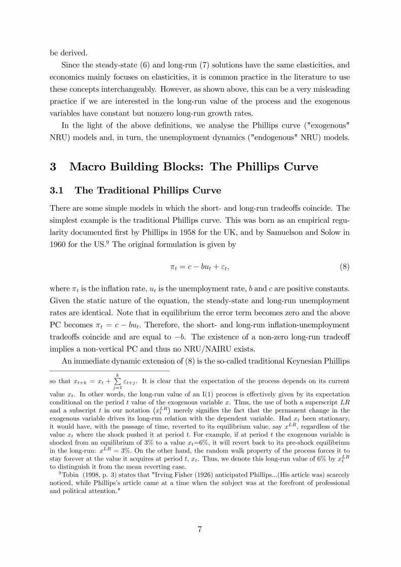
1960 for the US.9 The original formulation is given by

πt = c− but + εt, (8)

where πt is the inflation rate, ut is the unemployment rate, b and c are positive constants.

Given the static nature of the equation, the steady-state and long-run unemployment

rates are identical. Note that in equilibrium the error term becomes zero and the above

PC becomes πt = c − but. Therefore, the short- and long-run inflation-unemployment

tradeoffs coincide and are equal to −b. The existence of a non-zero long-run tradeoffimplies a non-vertical PC and thus no NRU/NAIRU exists.

An immediate dynamic extension of (8) is the so-called traditional Keynesian Phillips

so that xt+k = xt +kP

j=1εt+j . It is clear that the expectation of the process depends on its current

value xt. In other words, the long-run value of an I(1) process is effectively given by its expectationconditional on the period t value of the exogenous variable x. Thus, the use of both a superscript LRand a subscript t in our notation

¡xLRt

¢merely signifies the fact that the permanent change in the

exogenous variable drives its long-run relation with the dependent variable. Had xt been stationary,it would have, with the passage of time, reverted to its equilibrium value, say xLR, regardless of thevalue xt where the shock pushed it at period t. For example, if at period t the exogenous variable isshocked from an equilibrium of 3% to a value xt=6%, it will revert back to its pre-shock equilibriumin the long-run: xLR = 3%. On the other hand, the random walk property of the process forces it tostay forever at the value it acquires at period t, xt. Thus, we denote this long-run value of 6% by xLRtto distinguish it from the mean reverting case.

9Tobin (1998, p. 3) states that "Irving Fisher (1926) anticipated Phillips...(His article was) scarcelynoticed, while Phillips’s article came at a time when the subject was at the forefront of professionaland political attention."

7

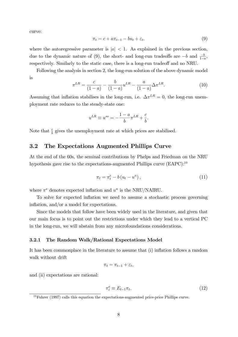
curve:

πt = c+ aπt−1 − but + εt, (9)

where the autoregressive parameter is |a| < 1. As explained in the previous section,

due to the dynamic nature of (9), the short- and long-run tradeoffs are −b and −b1−a ,

respectively. Similarly to the static case, there is a long-run tradeoff and no NRU.

Following the analysis in section 2, the long-run solution of the above dynamic model

is

πLR =c

(1− a)− b

(1− a)uLR − a

(1− a)∆πLR. (10)

Assuming that inflation stabilises in the long-run, i.e. ∆πLR = 0, the long-run unem-

ployment rate reduces to the steady-state one:

uLR ≡ uss = −1− a

bπLR +

c

b.

Note that cbgives the unemployment rate at which prices are stabilised.

3.2 The Expectations Augmented Phillips Curve

At the end of the 60s, the seminal contributions by Phelps and Friedman on the NRU

hypothesis gave rise to the expectations-augmented Phillips curve (EAPC):10

πt = πet − b (ut − un) , (11)

where πe denotes expected inflation and un is the NRU/NAIRU.

To solve for expected inflation we need to assume a stochastic process governing

inflation, and/or a model for expectations.

Since the models that follow have been widely used in the literature, and given that

our main focus is to point out the restrictions under which they lead to a vertical PC

in the long-run, we will abstain from any microfoundations considerations.

3.2.1 The Random Walk/Rational Expectations Model

It has been commonplace in the literature to assume that (i) inflation follows a random

walk without drift

πt = πt−1 + εt,

and (ii) expectations are rational:

πet ≡ Et−1πt, (12)

10Fuhrer (1997) calls this equation the expectations-augmented price-price Phillips curve.

8

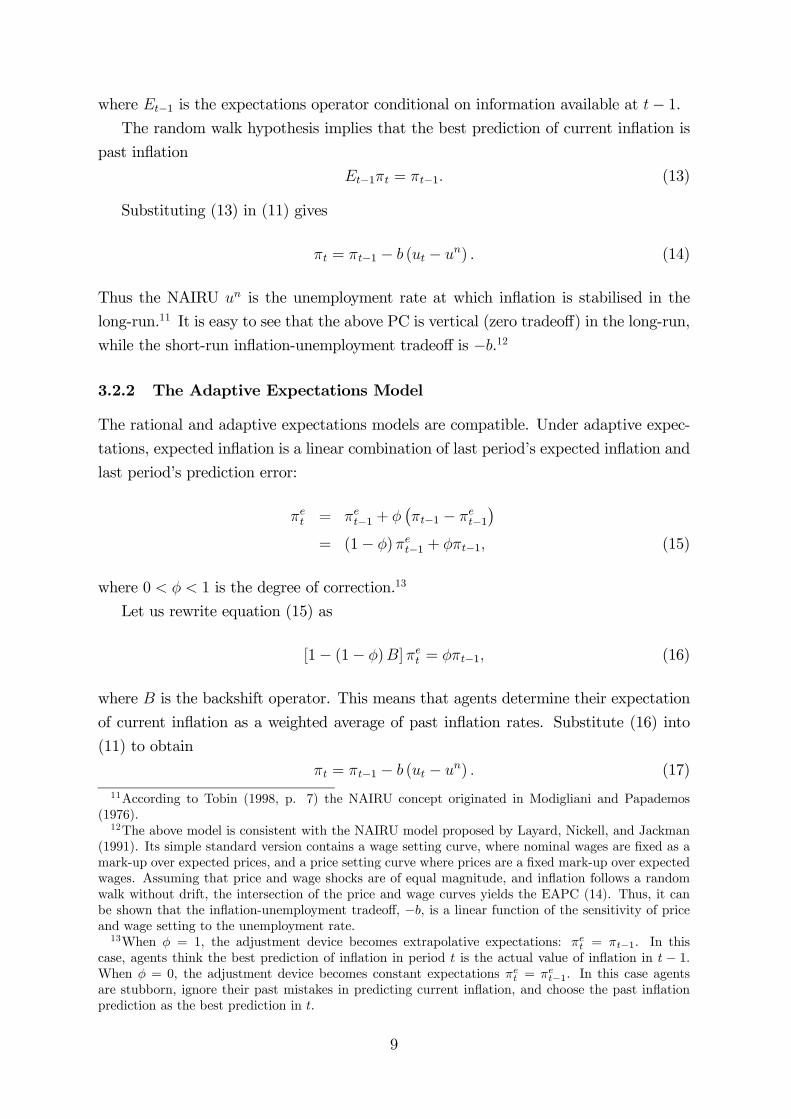
where Et−1 is the expectations operator conditional on information available at t− 1.The random walk hypothesis implies that the best prediction of current inflation is

past inflation

Et−1πt = πt−1. (13)

Substituting (13) in (11) gives

πt = πt−1 − b (ut − un) . (14)

Thus the NAIRU un is the unemployment rate at which inflation is stabilised in the

long-run.11 It is easy to see that the above PC is vertical (zero tradeoff) in the long-run,

while the short-run inflation-unemployment tradeoff is −b.12

3.2.2 The Adaptive Expectations Model

The rational and adaptive expectations models are compatible. Under adaptive expec-

tations, expected inflation is a linear combination of last period’s expected inflation and

last period’s prediction error:

πet = πet−1 + φ¡πt−1 − πet−1

¢= (1− φ)πet−1 + φπt−1, (15)

where 0 < φ < 1 is the degree of correction.13

Let us rewrite equation (15) as

[1− (1− φ)B]πet = φπt−1, (16)

where B is the backshift operator. This means that agents determine their expectation

of current inflation as a weighted average of past inflation rates. Substitute (16) into

(11) to obtain

πt = πt−1 − b (ut − un) . (17)

11According to Tobin (1998, p. 7) the NAIRU concept originated in Modigliani and Papademos(1976).12The above model is consistent with the NAIRU model proposed by Layard, Nickell, and Jackman

(1991). Its simple standard version contains a wage setting curve, where nominal wages are fixed as amark-up over expected prices, and a price setting curve where prices are a fixed mark-up over expectedwages. Assuming that price and wage shocks are of equal magnitude, and inflation follows a randomwalk without drift, the intersection of the price and wage curves yields the EAPC (14). Thus, it canbe shown that the inflation-unemployment tradeoff, −b, is a linear function of the sensitivity of priceand wage setting to the unemployment rate.13When φ = 1, the adjustment device becomes extrapolative expectations: πet = πt−1. In this

case, agents think the best prediction of inflation in period t is the actual value of inflation in t − 1.When φ = 0, the adjustment device becomes constant expectations πet = πet−1. In this case agentsare stubborn, ignore their past mistakes in predicting current inflation, and choose the past inflationprediction as the best prediction in t.

9

Therefore, the EAPC under adaptive expectations is identical to the EAPC under the

random walk/rational expectations assumption (14).

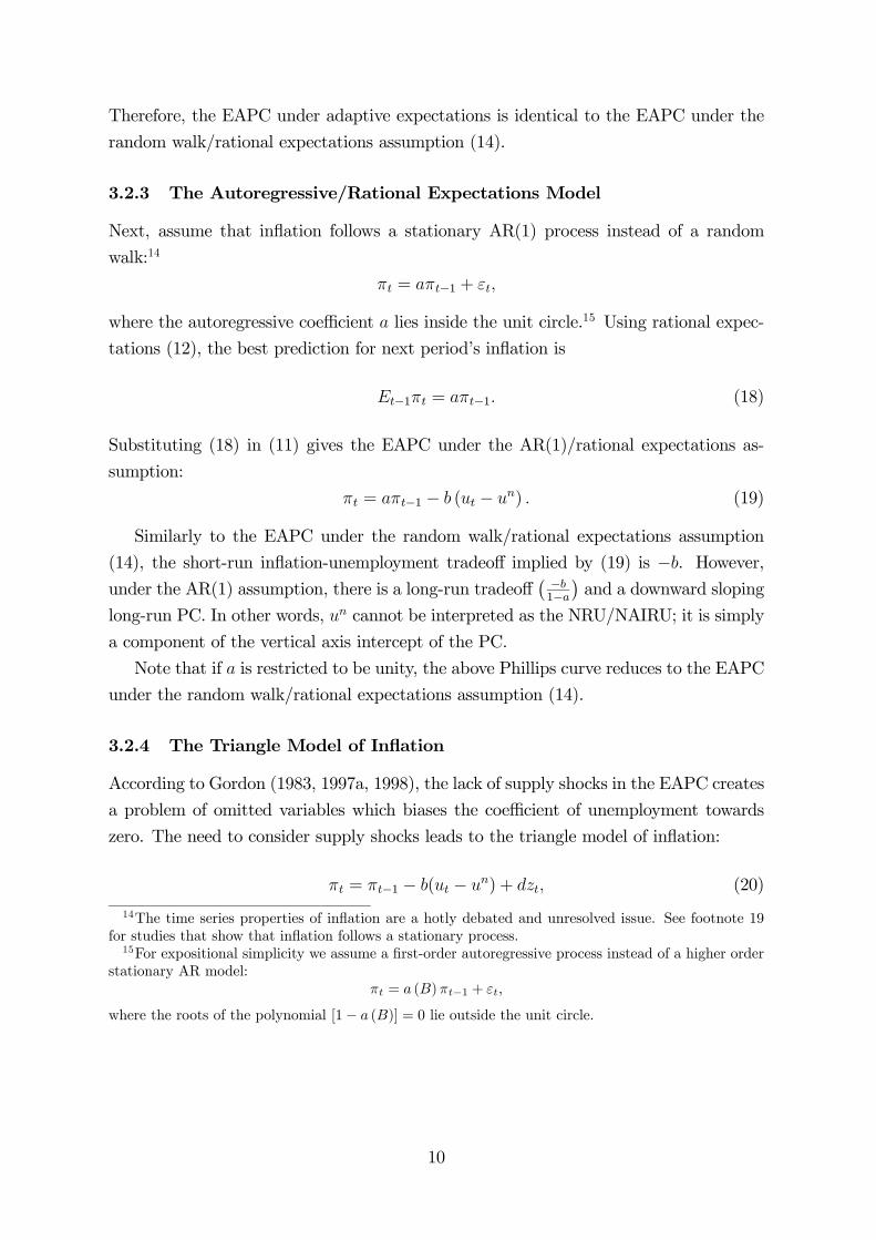
3.2.3 The Autoregressive/Rational Expectations Model

Next, assume that inflation follows a stationary AR(1) process instead of a random

walk:14

πt = aπt−1 + εt,

where the autoregressive coefficient a lies inside the unit circle.15 Using rational expec-

tations (12), the best prediction for next period’s inflation is

Et−1πt = aπt−1. (18)

Substituting (18) in (11) gives the EAPC under the AR(1)/rational expectations as-

sumption:

πt = aπt−1 − b (ut − un) . (19)

Similarly to the EAPC under the random walk/rational expectations assumption

(14), the short-run inflation-unemployment tradeoff implied by (19) is −b. However,under the AR(1) assumption, there is a long-run tradeoff

¡ −b1−a¢and a downward sloping

long-run PC. In other words, un cannot be interpreted as the NRU/NAIRU; it is simply

a component of the vertical axis intercept of the PC.

Note that if a is restricted to be unity, the above Phillips curve reduces to the EAPC

under the random walk/rational expectations assumption (14).

3.2.4 The Triangle Model of Inflation

According to Gordon (1983, 1997a, 1998), the lack of supply shocks in the EAPC creates

a problem of omitted variables which biases the coefficient of unemployment towards

zero. The need to consider supply shocks leads to the triangle model of inflation:

πt = πt−1 − b(ut − un) + dzt, (20)

14The time series properties of inflation are a hotly debated and unresolved issue. See footnote 19for studies that show that inflation follows a stationary process.15For expositional simplicity we assume a first-order autoregressive process instead of a higher order

stationary AR model:πt = a (B)πt−1 + εt,

where the roots of the polynomial [1− a (B)] = 0 lie outside the unit circle.

10

where lagged inflation captures the degree of nominal sluggishness, zt is a k × 1 vectorof supply shocks (e.g. productivity shocks), and d is a 1×k vector of parameters.16 The

"triangle" refers to the three factors that influence inflation: lags, demand, and supply.

The unemployment gap (ut − un) is a measure of excess demand which can alterna-

tively be proxied by: (i) the output gap, defined as the percentage deviation of actual

output with respect to potential output,17 and (ii) the capacity utilization gap, defined

as the difference between the degree of capacity utilization and its non accelerating

inflation rate (NAIRCU).

Observe that in (20) expectations are not explicitly considered since price inertia is

compatible with both rational and adaptive expectations. In this setting, the divergence

between the actual and the steady-state unemployment rate arises from unexpected infla-

tion and the supply-side shocks. Note that, although no assumption about expectations

is made, the triangle model (20) assumes that inflation follows a random walk.

Furthermore, it is easy to see that, like the previous standard versions of the EAPC

model, the Phillips curve is downward sloping in the short-run, vertical in the long-run,

and the NRU/NAIRU is equal to un.18

When the autoregressive coefficient in (20) is not restricted to unity (a 6= 1), thetriangle model is given by

πt = aπt−1 − b(ut − un) + dzt. (21)

For analytical purposes it is important to distinguish the following three cases arising

from the time series properties of the variables in the above (unrestricted) triangle model

(21):

1. If inflation is I(1), and excess demand and supply shocks are I(0), a balanced

equation can be obtained only if the restriction a = 1 is imposed. This is the case

of the conventional triangle model (20).

2. Inflation is I(1), excess demand and supply shocks are also I(1), and all variables

cointegrate. In this case the triangle model is dynamically stable, i.e. |a| < 1, andthus no NRU/NAIRU exists.

16For expositional ease, we use the above simple ARDL(1,0,0) instead of the general model

πt = a(B)πt−1 + b(B)xt + d(B)zt,

where a (1) = 1. That is, one root of the polynomial equation [1− a(B)] = 0 is unity while the rest lieouside the unit circle. This means that inflation follows an I(1) process. Also, without loss of generality,we ignore the error term.17Okun’s law links the unemployment and output gaps. Its simplest expression is (ut − un) =−θ (yt − yn), where y is the log of real output and yn its natural level.18This is because of the absence of shocks in the steady-state.

11

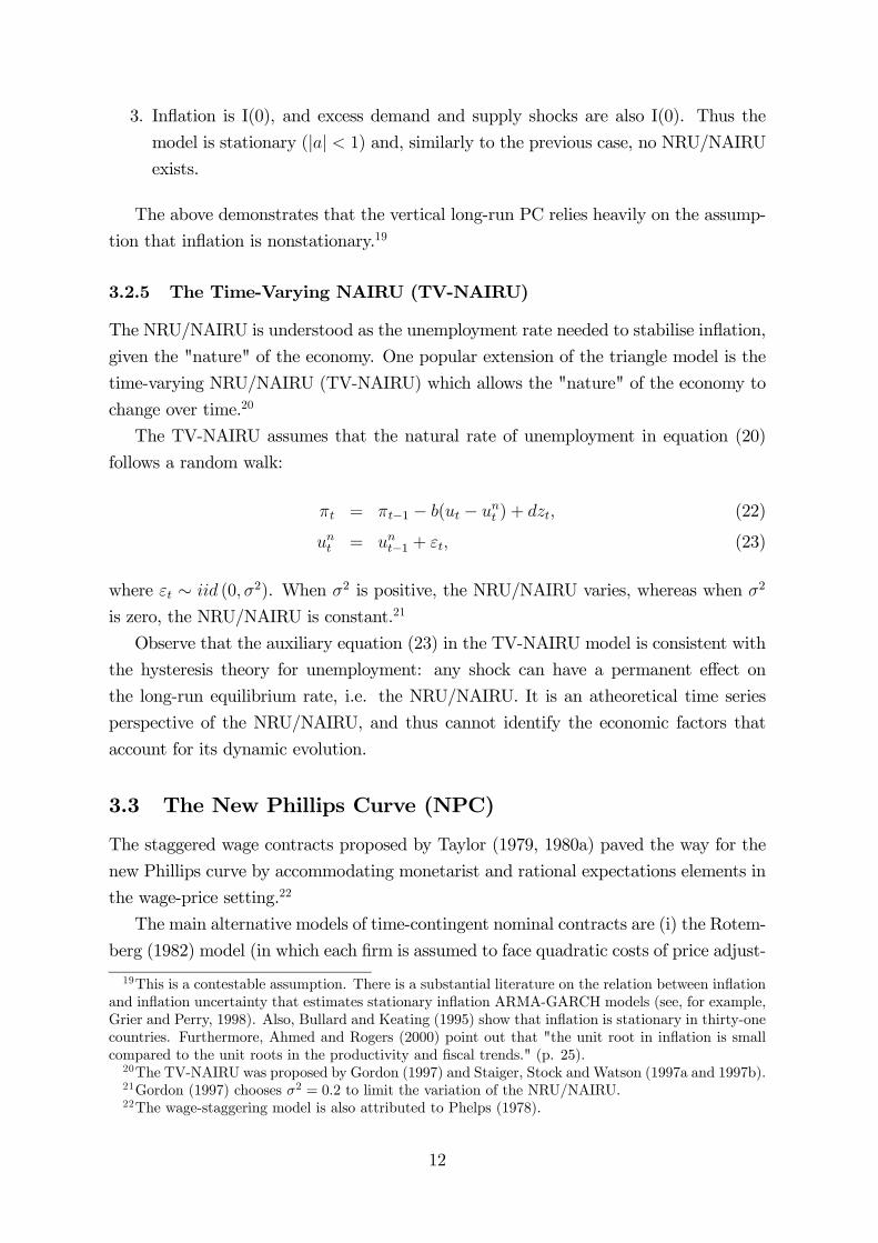
3. Inflation is I(0), and excess demand and supply shocks are also I(0). Thus the

model is stationary (|a| < 1) and, similarly to the previous case, no NRU/NAIRUexists.

The above demonstrates that the vertical long-run PC relies heavily on the assump-

tion that inflation is nonstationary.19

3.2.5 The Time-Varying NAIRU (TV-NAIRU)

The NRU/NAIRU is understood as the unemployment rate needed to stabilise inflation,

given the "nature" of the economy. One popular extension of the triangle model is the

time-varying NRU/NAIRU (TV-NAIRU) which allows the "nature" of the economy to

change over time.20

The TV-NAIRU assumes that the natural rate of unemployment in equation (20)

follows a random walk:

πt = πt−1 − b(ut − unt ) + dzt, (22)

unt = unt−1 + εt, (23)

where εt ∼ iid (0, σ2). When σ2 is positive, the NRU/NAIRU varies, whereas when σ2

is zero, the NRU/NAIRU is constant.21

Observe that the auxiliary equation (23) in the TV-NAIRU model is consistent with

the hysteresis theory for unemployment: any shock can have a permanent effect on

the long-run equilibrium rate, i.e. the NRU/NAIRU. It is an atheoretical time series

perspective of the NRU/NAIRU, and thus cannot identify the economic factors that

account for its dynamic evolution.

3.3 The New Phillips Curve (NPC)

The staggered wage contracts proposed by Taylor (1979, 1980a) paved the way for the

new Phillips curve by accommodating monetarist and rational expectations elements in

the wage-price setting.22

The main alternative models of time-contingent nominal contracts are (i) the Rotem-

berg (1982) model (in which each firm is assumed to face quadratic costs of price adjust-

19This is a contestable assumption. There is a substantial literature on the relation between inflationand inflation uncertainty that estimates stationary inflation ARMA-GARCH models (see, for example,Grier and Perry, 1998). Also, Bullard and Keating (1995) show that inflation is stationary in thirty-onecountries. Furthermore, Ahmed and Rogers (2000) point out that "the unit root in inflation is smallcompared to the unit roots in the productivity and fiscal trends." (p. 25).20The TV-NAIRU was proposed by Gordon (1997) and Staiger, Stock and Watson (1997a and 1997b).21Gordon (1997) chooses σ2 = 0.2 to limit the variation of the NRU/NAIRU.22The wage-staggering model is also attributed to Phelps (1978).

12

ment, which it minimises) and (ii) the particularly popular Calvo (1983) model (in which

each firm has to keep its price fixed until it receives a random “permission-to-adjust-

price” signal, and the probability of receiving this signal remains constant through time).

These alternatives however are problematic.

In Rotemberg’s approach, it is unclear why the cost of price change should be pos-

itively related to the magnitude of price change. In fact, the menu cost literature has

been built up on the explicit assumption that no such relation exists. Regarding Calvo’s

approach, it is obviously far-fetched to assume that a firm’s probability of price adjust-

ment is independent of how long it has been since its last price adjustment.

Nevertheless, the Calvo model is commonly used as a convenient algebraic shorthand

for the Taylor model.23 Goodfriend and King (1997, p.254) show that under intertem-

poral optimisation and certain conditions,24 Calvo’s setup broadly resembles that of

Taylor.

Below we first summarise Taylor’s wage-staggering model and then present and eval-

uate the standard sticky-price model of the NPC literature.

3.3.1 Wage-Staggering Contracts

The seminal contribution of Taylor’s work is that it gives an economic justification

to unemployment rate dynamics. It thus strengthens the case against the view that

the autoregressive nature of the unemployment rate is merely a statistical one - if one

could observe and include in the model all the relevant exogenous variables, lagged

unemployment terms would simply become statistically insignificant. Taylor used a

standard macro model with rational expectations and showed that wage staggering

alone induces unemployment to depend on its own lags.

In its simplest form, wage staggering assumes that nominal wages are fixed for two

periods and there are two contracts that are evenly staggered. The Taylor equation

postulates that the contract wage depends on past and expected future contract wages,

as well as current and future excess labour demand:

Wt = αWt−1 + (1− α)EtWt+1 + γ [αxt + (1− α)Etxt+1] + ωt, (24)

where the contract wage Wt is set at the beginning of period t for periods t and t+ 1,

xt denotes excess demand, Et(·) is the expectation of the variable conditional uponinformation available at time t, and the supply shock ωt is a white noise process. (All

variables are in logs.) The demand sensitivity parameter γ describes how strongly wages

23Also, as Goodfriend and King (1997) point out (p. 249), New Keynesian economists who felt uneasyabout wage-staggering contracts found Calvo’s price-setting model quite attractive.24These conditions are low inflation, constant elasticity of demand, and small variations in adjustment

patterns.

13

are influenced by demand. Note that the only restriction that needs to be imposed on

the backward- and forward-looking weights is that they add up to unity - they do not

have to be equal to one another.25

Assuming constant returns to labour in the production function, the (log) price level

is a constant markup over the average wage: Pt =12(Wt +Wt−1) . Taylor (1980a, p.4-5)

closed his macro model by assuming that excess labour demand is proportional to the

output gap and output gap depends on detrended real money balances. The supply and

demand sides of the economy are equilibrated through the wage contract equation (24).

Taylor (1980a) shows that the rational expectations solution of the above two-period

contract wage model yields an ARMA(1,1) equation for the unemployment rate.

3.3.2 The Sticky-Price Model of the NPC

Taylor’s and Calvo’s wage/price-setting models were subsequently reformulated into

what has become known as the workhorse model of the New (Keynesian) Phillips

Curve.26

The NPC explains current inflation πt by expected inflation one period ahead and a

forcing variable xt:

πt = βEtπt+1 + γ (1 + β) xt, (25)

where xt denotes excess demand or marginal costs (i.e., unemployment rate, (log) output

gap, or (log) wage share), γ is the “demand sensitivity parameter” (a constant), and

inflation is the first difference of the log price level, πt ≡ Pt − Pt−1. In contrast to the

"old" PC, the NPC is forward-looking and past inflation rates only matter if they are

correlated with the rational expectation of next period’s inflation rate.

The New Phillips curve (25) is simply a reparameterisation of the following price-

setting equation:27

Pt = αPt−1 + (1− α)EtPt+1 + γxt, (26)

where the discount parameter α = 11+β

(the discount factor β = 11+r

, and r is the

discount rate).28 The lagged price term captures nominal rigidities and so equation (26)

clearly implies price inertia: a demand shock affects the price level for many periods.

Throughout the past decade, the New Phillips curve (25) has been receiving a lot

of theoretical and empirical support.29 It is certainly true to say that the conventional

25However, the wage-staggering specification in Taylor (1980a) attaches equal weights to thebackward- and forward-looking variables.26See, for example, Roberts (1995), Gali and Gertler (1999), and Mankiw and Reis (2002).27To obtain the New Keynesian Phillips curve (25), subtract from both sides of the price-setting

eq. (26) (i) Pt−1 to get πt − (1− α)Pt−1 = (1− α)EtPt+1 + γxt, and (ii) (1− α)Pt so that απt =(1− α)Etπt+1 + γxt.28We discuss this result in detail in Section 5.29See Gali and Gertler (1999), Svensson (2000), Gali, Gertler, and Lopez-Salido (2001), and the

14

analyses of the NPC are broadly compatible with the NAIRU: When the interest rate

is zero (so that α = 1/2 and β = 1), equation (25) reduces to the standard textbook

version of the Phillips curve, for which there is no long-run tradeoff between inflation

and unemployment/output. Since β ≈ 1, it is generally taken for granted that the long-run Phillips curve is almost vertical. As we will show in Section 5, the long-run slope is

a function of both β and γ and it is highly sensitive to the value of γ.

The choice of the forcing variable is crucial when estimating the inflation dynamics

associated with the Phillips curve. Galí and Gertler (1999), Galí, Gertler and López-

Salido (2001) estimate (25) with GMM and find evidence in support of the NPC only

when they use labour income share (rather than the output gap or unemployment) as

the forcing variable. As Galí and Gertler indicate, the resulting equation can be called

an inflation dynamics equation, rather than a Phillips curve, since the latter is meant

to describe the relation between inflation and some measure of the magnitude of macro-

economic activity. It is important to note that the labour income share is essentially the

wage-productivity gap.30 Thus the positive and significant relation between inflation

and labour share evidenced in the above papers, is simply a reflection of the downward

pressure put on inflation when wage gains trail productivity gains.

The "Forcing" Variable The use of term "forcing" variable in the single-equation

standard and hybrid NPC models suggests the exogeneity of xt. (The hybrid NPC is

given below.) But in the context of all reasonable macro models of the Phillips curve,

xt is not exogenous. Rather, inflation πt and the real variable xt are both endogenous

responding to economic policy changes. In Section 5 we show that the endogeneity of

the "forcing" variable has important implications for both the persistence of inflation

and the slope of the PC in the long-run.

Karanassou, Sala, and Snower (2002, 2005) examine, theoretically and empirically,

the inflation-unemployment tradeoff in the context of multi-equation systems containing

both the Phillips curve as well as the relation between the real variable and the policy

shock. Bårdsen, Jansen and Nymoen (2002, 2004) put forward an econometric evalua-

tion of the standard and hybrid NPC’s and emphasize the importance of modelling a

system that includes the forcing variable as well as the rate of inflation.

special issue on the NPC of the Journal of Monetary Economics (2005).30The labour share can be written as

wagesGDP

=wages/employeesGDP/employees

=wage

productivity.

So the labour share is equivalent to the ratio of average real wage and productivity. If, say, a 10%productivity gain is accompanied by a 10% growth in the average real wage, then the wage productivitygap is zero. On the other hand, the lower the wage growth, the more wages trail productivity gainsand thus the higher is the wage-productivity gap. We should also note that in the literature the labourincome share is used as a proxy for real marginal costs.

15

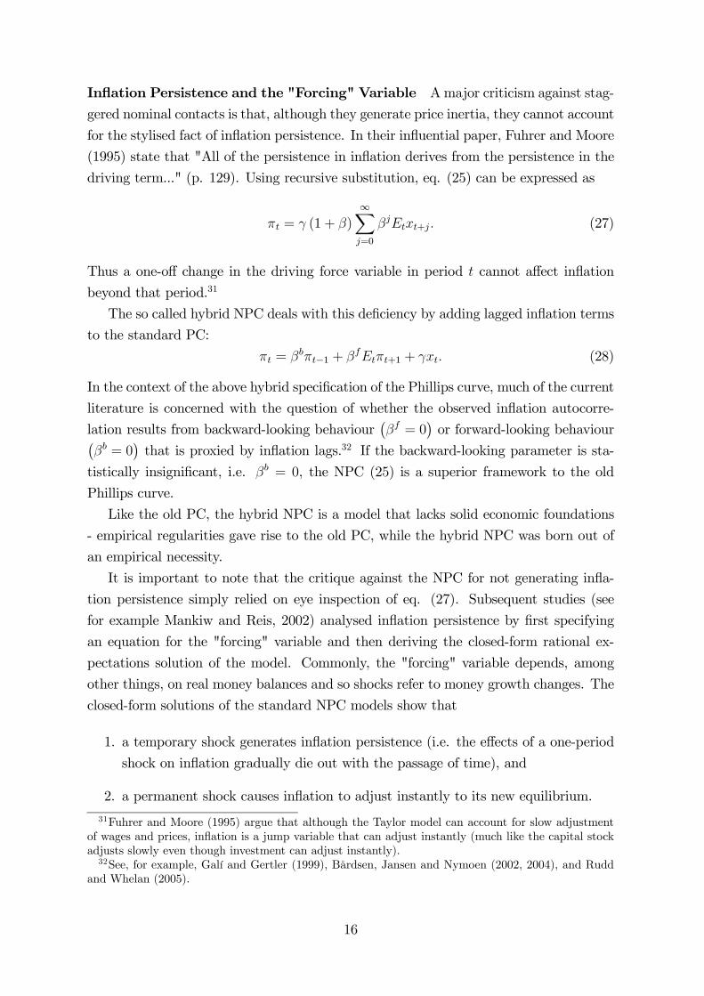
Inflation Persistence and the "Forcing" Variable Amajor criticism against stag-

gered nominal contacts is that, although they generate price inertia, they cannot account

for the stylised fact of inflation persistence. In their influential paper, Fuhrer and Moore

(1995) state that "All of the persistence in inflation derives from the persistence in the

driving term..." (p. 129). Using recursive substitution, eq. (25) can be expressed as

πt = γ (1 + β)∞Xj=0

βjEtxt+j. (27)

Thus a one-off change in the driving force variable in period t cannot affect inflation

beyond that period.31

The so called hybrid NPC deals with this deficiency by adding lagged inflation terms

to the standard PC:

πt = βbπt−1 + βfEtπt+1 + γxt. (28)

In the context of the above hybrid specification of the Phillips curve, much of the current

literature is concerned with the question of whether the observed inflation autocorre-

lation results from backward-looking behaviour¡βf = 0

¢or forward-looking behaviour¡

βb = 0¢that is proxied by inflation lags.32 If the backward-looking parameter is sta-

tistically insignificant, i.e. βb = 0, the NPC (25) is a superior framework to the old

Phillips curve.

Like the old PC, the hybrid NPC is a model that lacks solid economic foundations

- empirical regularities gave rise to the old PC, while the hybrid NPC was born out of

an empirical necessity.

It is important to note that the critique against the NPC for not generating infla-

tion persistence simply relied on eye inspection of eq. (27). Subsequent studies (see

for example Mankiw and Reis, 2002) analysed inflation persistence by first specifying

an equation for the "forcing" variable and then deriving the closed-form rational ex-

pectations solution of the model. Commonly, the "forcing" variable depends, among

other things, on real money balances and so shocks refer to money growth changes. The

closed-form solutions of the standard NPC models show that

1. a temporary shock generates inflation persistence (i.e. the effects of a one-period

shock on inflation gradually die out with the passage of time), and

2. a permanent shock causes inflation to adjust instantly to its new equilibrium.

31Fuhrer and Moore (1995) argue that although the Taylor model can account for slow adjustmentof wages and prices, inflation is a jump variable that can adjust instantly (much like the capital stockadjusts slowly even though investment can adjust instantly).32See, for example, Galí and Gertler (1999), Bårdsen, Jansen and Nymoen (2002, 2004), and Rudd

and Whelan (2005).

16

Therefore, a widely recognised deficiency of the NPC is that it implies that inflation

is a jump variable - following a permanent increase (decrease) in money growth at period

t, inflation jumps up (down) instantaneously to its new long-run value.

This is exactly what is meant by the, somehow confusing, statement that "the NPC

does not generate inflation persistence". It was precisely because of this perceived

deficiency of the NPC (or sticky-price Phillips curve) that Mankiw and Reis (2002)

proposed the sticky-information PC which can generate sufficient inflation persistence.

It is also because of this inability of the standard NPC that Blanchard and Gali (2005)

propose a PC model that incorporates real wage rigidities. As they put it, p. 4, "the

introduction of real wage rigidities overcomes a well known empirical weakness of the

standard NK model...namely, its lack of inflation inertia - which we define as the degree

of inflation persistence beyond that inherited from the output gap itself."

4 Labour Economics Building Blocks: Endogenous

NRU Approaches and Unemployment Dynamics

The endogenous NRU approaches seek to explain movements in the long-run equilib-

rium (or natural rate) of unemployment, by distinguishing two components. First,

the so called "business cycle," i.e. the high-frequency (or conjunctural) unemployment

movements which are induced by the effects of temporary shocks disrupting equilib-

rium. Second, the so called "trend," i.e. the low-frequency (or long-run equilibrium)

movements which arise from structural changes in the unemployment determinants.

The theories discussed below endogenise the natural rate (or long-run equilibrium)

of unemployment and model unemployment dynamics either via a single equation, i.e.

traditional dynamics, or via a labour market system, i.e. interactive dynamics. Tradi-

tional dynamics are exemplified by the structuralist theory (ST), whereas interactive

dynamics are exemplified by the chain reaction theory (CRT).

4.1 Traditional Dynamics: The Structuralist Theory (ST)

The aim of the structuralist theory is to disclose “the nonmonetary mechanisms through

which various nonmonetary forces are capable of propagating slumps and booms in the

contemporary world economy.”33 Its main characteristic is the analysis of the unemploy-

ment rate via dynamic single-equation models. In this context, the NRU is the attractor

of the stationary actual unemployment rate which can only temporarily deviate from

its natural rate.33Phelps (1994, p. 1)

17

Thus, in line with conventional wisdom, the ST views the "trend" and "business

cycle" components of unemployment as independent. The objective of the ST is to

identify the driving forces of the "trend," i.e. the NRU. It is important to note that

the ST cannot analyse the effects of permanent shocks on unemployment, since the

stationary single-equation models can only feature temporary labour market shocks.

From the structuralist perspective, the trajectory of unemployment is determined by

the structure of the economy, rather than by labour market lags (i.e. employment, real

wage, and labour force lags). This structure is made up of two components: (i) firm’s

assets, which drive the labor demand; and (ii) the income from the worker’s wealth,

which drives the wage setting curve. Firm’s assets include investments in employees,

customers and tangible capital, whereas the income from worker’s wealth include all

returns from their private wealth - either real or financial (i.e., in the form of assets) -

and from their social wealth (all entitlements from the state). In recent papers, however,

asset prices became the centerpiece variable of the structuralist theory.34 In other words,

asset prices are the driving force determining the trajectory of the moving natural rate

of unemployment.

When the ST equations include the acceleration of inflation as an explanatory vari-

able, they are compatible with the weak-form NRU. Essentially, they can be described

as augmented PC models where the time-varying NRU changes are attributed to fun-

damentals.35

Phelps’ (1994, ch. 17) provides the estimates of a single-equation unemployment rate

model for 17 OECD countries which, according to Phelps and Zoega (1998, p. 787), can

be thought as a “first step in testing a moving-natural-rate theory of unemployment.”

The explanatory variables in the Phelps (1994) model can be grouped in three sets:

(i) unemployment lags; (ii) country-specific variables, such as total capital stock,36 real

public debt, real government spending, some tax variables (direct taxes, payroll taxes),37

other institutional variables (replacement rate, duration of unemployment benefits),

price markups induced by exchange rates, and some demographic/labour-supply vari-

able (like the proportion of population between 20 and 24 years old)38; and (iii) world

variables, such as the world real interest rate and the world price of oil.

The main conclusions drawn from the Phelps (1994) empirical analysis are that the

34See Phelps (1999), Fitoussi et al. (2000) and Phelps and Zoega (2001).35See Phelps and Zoega (1998). Coakley, Fuertes and Zoega (2001) test the structuralist theory in

UK, US and Germany and find support for it using a nonlinear TAR model with a one-time shift inequilibrium unemployment.36Normalised by another variable so that its trend is removed.37Value added taxes are not considered since they affect more or less proportionately wage and

nonwage income.38In their 1997 work, changes in the teenage share are found to be insufficiently large to explain the

US unemployment movements, but the educational attainment of the different cohorts is outlined asan important factor to explain the downward trend in the natural rate.

18

oil price was the principal determinant of the rise in unemployment in the 70s, the real

interest rates was the main driving force of unemployment in the 80s, and direct/payroll

taxes were important in explaining the diverse experiences of the OECD countries.39

The pool of explanatory variables was augmented in subsequent works of the struc-

turalist theorists. For example, in Phelps and Zoega (1997, 1998) three additional

country-specific factors influencing the unemployment path are the slowdown of produc-

tivity (since the mid 70s), the share of social expenditures in GDP, and the educational

composition of the labour force (in the US and UK).

Phelps and Zoega (1998) also examine the role played by the real exchange rate

appreciation in France and Germany, resulting from their tight monetary policies, and

depreciation in the periphery of the EU (Scandinavia, the Netherlands and the UK).

The authors argue that exchange rate fluctuations, despite being a monetary and not a

structural factor, were important for the evolution of unemployment during the 90s.

Furthermore, Phelps (1999), Fitoussi et al. (2000) and Phelps and Zoega (2001)

incorporate the role of asset valuation in the analysis of the unemployment problem.

Phelps (1999) concludes that asset prices help to explain employment growth in the US,

and Fitoussi et al. (2000) argue that asset prices are the mechanism whereby the "New

Economy" (or other developments capable of boosting firms’ expected profitability, like

globalization or biogenetics) enhance employment. The later study also tests three

competing hypotheses for explaining the booming 90’s of the OECD countries - labour

market reforms, monetary theses and the "new economy" - and gives support to the

"new economy" hypothesis.

Finally, for the same group of OECD countries, Phelps and Zoega (2001) argue

that the long swings in economic activity result from the changes in expected future

productivity which can be proxied by the swings in the stock market.

4.2 Interactive Dynamics: The Chain Reaction Theory (CRT)

We will show in Section 5 that the dynamics of inflation and unemployment are inti-

mately related. This calls for a modelling procedure that can jointly determine inflation

and unemployment. An interactive dynamics approach can unify the macro literature

that models inflation dynamics with the labour literature that models the evolution of

unemployment.

The chain reaction theory of unemployment (CRT) is an interactive dynamics ap-

proach applied to the labour market.40 To fully appreciate the value added of interactive

39In Phelps and Zoega (1998) the crucial effect of interest rates is further extended to the 90s, andthe effect of taxes restricted mainly to the 60s and 70s.40The CRT was developed by Karanassou and Snower (1996). See also Karanassou and Snower

(1998).

19

dynamics, we explain the workings of the CRT and then compare it with the traditional

dynamics approach of the structuralist theory.

The first salient feature of the CRT is the use of dynamic multi-equation systems

to analyse the trajectory of the unemployment rate.41 In the context of autoregressive

multi-equation models, movements in unemployment can be viewed as "chain reactions"

of responses to labour market shocks, working their way through systems of interacting

lagged adjustment processes.

These lagged adjustment processes are well documented in the literature and refer,

among others, to: (i) employment adjustments arising from labour turnover costs (hir-

ing, training and firing costs), (ii) wage/price staggering, (iii) insider membership effects,

(iv) long-term unemployment effects, and (v) labour force adjustments. By identifying

the various lagged adjustment processes, the CRT can explore their interactions and

quantify the potential complementarities/substitutabilities among them.

According to the CRT, the NRU is not a reference point for the actual unemployment

rate when the long-run growth rates of the exogenous variables are nonzero constants.42

This is in stark contrast with the traditional dynamics models of the ST where the

natural rate is the attractor of unemployment.

This is an important point and we illustrate it with the following simple model of

labour demand and supply equations:

nt = α1nt−1 + β1kt, (29)

lt = α2lt−1 + β2zt, (30)

where nt denotes employment, lt is labour force, kt is capital stock, zt is working age

population, the autoregressive parameters are 0 < α1, α2 < 1, and the β’s are positive

constants. All variables are in logs; we ignore the error terms for ease of exposition. We

can plausibly assume that both capital stock and working age population are growing

variables with growth rates that stabilise in the long-run.43

According to (7), the long-run solutions of the labour demand and supply equations

(29)-(30) are

nLRt =β1

1− α1kLRt −

α1(1− α1)

∆nLR, (31)

lLRt =β2

1− α2zLRt −

α2(1− α2)

∆lLR, (32)

41Karanassou, Sala, and Snower (2004) apply the CRT to explain the evolution of the EU unem-ployment rate. Bande and Karanassou (2006) apply the CRT to explain regional unemployment ratedisparities in Spain.42See Karanassou and Snower (1997).43Observe that when all variables are I(1), the labour demand and supply equations (29)-(30) imply

the cointegrating vectors (1, − β1/ (1− α1)), (1, − β2/ (1− α2)), respectively.

20

The unemployment rate (not in logs) is44

ut = lt − nt. (33)

Note that unemployment stabilises in the long-run, i.e. ∆uLR = 0, when ∆lLR =

∆nLR. In other words, for unemployment stability in the long-run, the growth rate of

employment should be equal to the growth rate of labour force, say g. We can also

express the restriction in terms of the long-run growth rates of the exogenous variables:

β11− α1

∆kLR =β2

1− α2∆zLR = g. (34)

Subtracting (32) from (31) and using the above restriction gives the following long-

run unemployment rate equation:

uLR =

∙β2

1− α2zLRt −

β11− α1

kLRt

¸+

∙(α1 − α2) g

(1− α1) (1− α2)

¸, (35)

where the first term in square brackets measures the NRU and the second term captures

frictional growth, i.e., the interplay between growth and the lagged adjustment processes.

The long-run value¡uLR

¢towards which the unemployment rate converges reduces

to the NRU only when frictional growth is zero - i.e. either when the exogenous variables

do not grow or when the labour demand and supply equations have identical dynamic

structures. Therefore, the NRU ceases to serve as an attractor for the unemployment

rate under frictional growth. Frictional growth can arise only in interactive dynamics

models. In the single equation models of the structuralist theory, the unemployment

rate converges to the NRU. As explained in Section 2, this is given by the steady-state

solution (6).

The second salient feature of the CRT is that it explicitly distinguishes between

temporary and permanent shocks and defines measures for the after-effects of such

shocks.45 For a temporary shock occurring at period t, unemployment persistence (σ)

is the sum of its responses for all periods in the aftermath of the shock (t+ j, j ≥ 1):

σ ≡∞Xj=1

Rut+j, (36)

where the series Rut+j, j ≥ 0 defines the unemployment impulse response function to the

44Since labour force and employment are in logs, we can approximate the unemployment rate bytheir difference.45See Karanassou and Snower (1998) for definitions of temporal as well as quantitative measures of

persistence and responsiveness and their application. See also Pivetta and Reis (2004) for a discussionof various persistence measures.

21

shock.46

If the unemployment rate model is static, then the shock is absorbed instantly and

so persistence is zero (σ = 0). If it is dynamically stable, then the effects of the shock

gradually die out and persistence is a finite quantity. Finally, if unemployment displays

hysteresis, then the temporary shock has a permanent effect and thus σ =∞.On the other hand, unemployment responsiveness measures the cumulative unem-

ployment effect of a permanent shock when unemployment does not adjust immediately

to its new long-run equilibrium. In particular, suppose that the economy at period t,

in an initial zero long-run equilibrium,47 is perturbed by a permanent unit shock. The

unemployment responsiveness is the sum of the differences through time between the ac-

tual unemployment rate and the new (post-shock) long-run equilibrium unemployment

rate:

ρ ≡∞Xj=0

£Rut+j − 1

¤, (37)

If unemployment responds instantaneously to the shock and jumps to its new long-

run equilibrium, then ρ = 0, i.e. unemployment is perfectly responsive. If unemployment

responds only gradually, so that the short-run unemployment effects of the shock are

less than the long-run effect (undershooting), then unemployment is under-responsive

and ρ < 0. Finally, unemployment can overshoot its long-run equilibrium. If the total

amount of overshooting exceeds the total amount of undershooting, then unemployment

is over-responsive (r > 0) .

The third salient feature of the CRT is the significant effect of capital stock on the

long-run equilibrium of unemployment.

This is in sharp contrast to the influential form of the literature asserting that poli-

cies that shift upward the time path of capital stock have no long-run effect on the

unemployment rate (see Layard, Nickell, and Jackman 1991). This view derives from

the observation that the unemployment rate is trendless in the long-run. Other influen-

tial forms of the literature have dealt with this stylised fact in two ways. Phelps (1994,

ch. 17), and Fitoussi et al. (2000) argue that the long-run unemployment rate can be

influenced by trendless transformations of the capital stock (for example, the unemploy-

ment rate may depend on the capital labour ratio). This is also supported by Rowthorn

(1999).48 Gordon (1997b) argues that a decrease in the growth rate of capital stock

leads to an increase in the unemployment rate. Modigliani (2000) shows that there is a

strong negative correlation between the investment and unemployment rates - this was

46In other words, Rut+j , j ≥ 0, denote the coefficients of the infinite moving average representation of

unemployment with respect to the shock.47This assumption is only made for expositional simplicity.48He argues that the capital stock does not affect the long-run unemployment rate in the Layard-

Nickell-Jackman model only because this model assumes a Cobb-Douglas production function, so thatthe elasticity of substitution between labour and capital is unity.

22

dubbed the "Modigliani puzzle" by Blanchard (2000, p. 140). Blanchard (2005) claims

that capital accumulation has influenced the evolution of European unemployment rate

over three decades. On the other hand, Malley and Moutos (2001) show that unemploy-

ment rate is affected in the long-run when domestic and foreign capital stocks grow at

unequal rates.

Karanassou and Snower (2004a) argue that there is no reason to believe that the

labour market alone is responsible for ensuring that the unemployment rate is trendless

in the long-run. In general, equilibrating mechanisms in the labour market and other

markets are jointly responsible for this phenomenon. Thus restrictions on the relation-

ships between the long-run growth rates (as opposed to the levels) of capital stock and

other growing exogenous variables are sufficient for this purpose.49

4.3 Comparing the Two Approaches

As discussed in the previous sections, while the structuralist theory models the unem-

ployment rate using traditional dynamics, the chain reaction theory uses interactive

dynamics and derives the reduced form unemployment rate equation. In this context,

the term "reduced form" means that the parameters of the equation are not estimated

directly - they are simply some nonlinear function of the parameters of the underlying

labour market system.

Generally, the ST postulates that the unemployment rate is a function of its own

lags and a set of exogenous variables. Since the unemployment rate is a nontrended

variable, the ST is restricted to use exogenous variables which do not display a trend.

This restriction does not apply to the CRT - the only requirement is that each of the

equations of the trended endogenous variables (e.g. employment, real wage, labour force,

etc.) is balanced by the set of its explanatory variables.

A further constraint of the structuralist theory is that it cannot analyse the responses

of unemployment to permanent shocks, since these are incompatible with the stationarity

property of the exogenous variables.

Finally, it can be shown that if the ST single-equation model and each equation of

the CRT multi-equation model have all identical regressors, then the two estimation

procedures will yield identical results.50 In this case, it makes no difference whether

one estimates unemployment rate directly via the ST single equation or via the reduced

form equation of the CRT system.

However, in structural labour market systems, it is generally not the case that each

constituent equation has the same regressors. Thus it becomes impossible for the re-

gressors of the ST model to be identical with the regressors in each equation of the CRT

49As an example consider the above labour market model (29)-(30) and the restriction (34) .50See Karanassou, Sala, and Snower (2003b).

23

model. Then the ST single-equation model can no longer be viewed as an unbiased

summary of the CRT multi-equation model. Rather, the detailed economic interactions

portrayed in the CRT model (including the dynamic interactions among the various

lagged adjustment processes) can no longer be captured in the ST single-equation model.

Generally, the CRT postulates that the evolution of unemployment is driven by

the interplay of lagged adjustment processes and the spillover effects within the labour

market system. Spillover effects arise when shocks to a specific equation feed through the

labour market system. The label "shocks" refers to changes in the exogenous variables.

To illustrate the workings of the CRT consider the following simple system of labour

demand, wage setting, and labour supply equations: 51

nt = α1nt−1 − γwt + β1kt, (38)

wt = α2wt−1 − δut + β2bt, (39)

lt = zt, (40)

where nt is employment, wt is real wage, and lt is labour force, the autoregressive para-

meters are 0 < α1, α2 < 1, γ, δ,and β’s are positive constants, kt is real capital stock, btis real benefits, and zt is working age population. As in the previous section, all variables

are in logs and we ignore the error terms for expositional ease. The unemployment rate

is given by (33).

When γ and δ are nonzero, all labour market shocks generate spillover effects. If

δ = 0, i.e. unemployment does not influence wages, then labour demand and supply

shocks do not spillover to wages. If γ = 0, i.e. labour demand is completely inelastic

with respect to wages, then shocks to wage setting do not spillover to unemployment. In

this case, the influence of the exogenous variables (kt, bt, and zt) on unemployment can

be measured through individual analysis of their respective equations. In other words,

the main feedback mechanism in this model is provided by the wage elasticity of labour

demand.

Let us rewrite the labour demand and real wage equations (38)-(39) as

(1− α1B)nt = −γwt + β1kt, (41)

(1− α2B)wt = −δut + β2bt, (42)

where B is the backshift operator. Substitution of (42) into (41) gives

(1− α1B) (1− α2B)nt = γδut + (1− α2B)β1kt − γβ2bt. (43)

51For more general models see Henry, Karanassou, and Snower (2000), and Karanassou, Sala, andSnower (2003b).

24

Next, rewrite the labour supply (40) as

(1− α1B) (1− α2B) lt = (1− α1B) (1− α2B) zt. (44)

Finally, subtract from (44) the labour demand eq. (43) to get the reduced form

unemployment rate equation:

[γδ + (1− α1B) (1− α2B)]ut = − (1− α2B)β1kt + γβ2bt + (1− α1B) (1− α2B) zt.

(45)

Note that the above equation is dynamically stable since (i) products of polynomials

in B which satisfy the stability conditions are stable, and (ii) linear combinations of

dynamically stable polynomials in B are also stable.

Alternatively, the reduced form unemployment rate equation (45) can be written as

ut = φ1ut−1 − φ2ut−2 − θk0kt + θbbt + θzzt + θk1kt−1 − φ1zt−1 + φ2zt−2 (46)

where φ1 =α1+α21+γδ

, φ2 =α1α21+γδ

, θk0 =β11+γδ

, θb =γβ21+γδ

, θz =1

1+γδand θk1 =

α21+γδ

.

The reduced form unemployment rate (46) portrays the following characteristics of

the CRT. First, the autoregressive parameters φ1 and φ2 embody the interplay of the

employment and wage setting adjustment processes (α1 and α2, respectively).

Second, the coefficients θk0, θb, and θz represent the short-run elasticities of unem-

ployment with respect to capital stock, benefits, and working age population, respec-

tively. The short-run elasticities are a function of the feedback mechanisms that give

rise to the spillover effects.

Third, the lag structure of the shocks in the reduced form equation emphasizes the

interplay of the lagged adjustment processes and the spillover effects.

A stationary, I(0), exogenous variable gives rise to a temporary shock and thus gen-

erates unemployment persistence which is measured by equation (36). It is important to

note that the sum of persistence and the short-run elasticity gives the long-run elasticity

of unemployment with respect to the specific variable.52

On the other hand, a nonstationary, I(1), exogenous variable gives rise to a per-

manent shock and thus generates unemployment responsiveness which is measured by

equation (37).

Recall that, in applied work the NRU is the equilibrium unemployment rate at

which there is no tendency for this rate to change at any time t, given the permanent

component values of the levels/growth rates of the exogenous variables at that time (see

52This relation is a very handy way to compute numerically the long-run elasticities in an interactivedynamics model.

25

Section 2). In this sense, it represents the unemployment that would be achieved once

all the lagged adjustment processes have been completed in response to the permanent

components of the exogenous variables.

Thus, the NRU is computed by setting B equal to unity in the CRT equation (45):

unt =(θz − φ1 + φ2) ezt + θbebt − (θk0 + θk1)ekt

1− φ1 + φ2, (47)

where thee above the variable denotes its permanent component. The estimates of theNRU will, by definition, reflect the interpretation of which changes in the exogenous

variables were permanent and which were temporary.

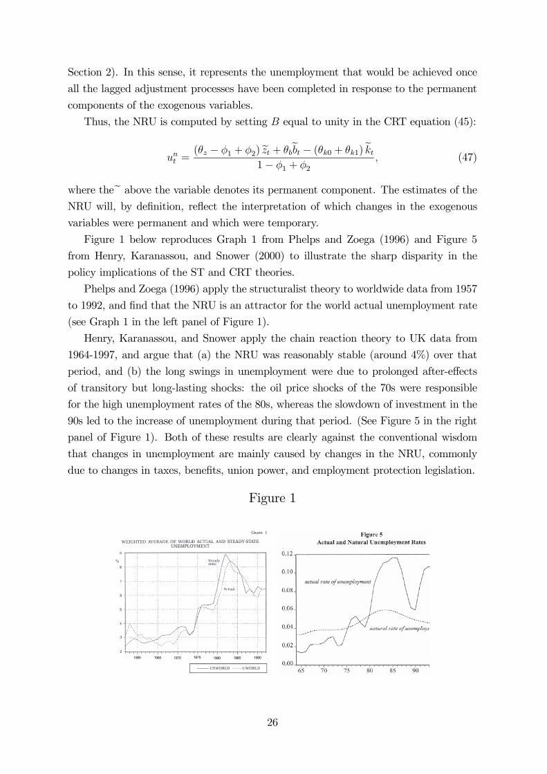
Figure 1 below reproduces Graph 1 from Phelps and Zoega (1996) and Figure 5

from Henry, Karanassou, and Snower (2000) to illustrate the sharp disparity in the

policy implications of the ST and CRT theories.

Phelps and Zoega (1996) apply the structuralist theory to worldwide data from 1957

to 1992, and find that the NRU is an attractor for the world actual unemployment rate

(see Graph 1 in the left panel of Figure 1).

Henry, Karanassou, and Snower apply the chain reaction theory to UK data from

1964-1997, and argue that (a) the NRU was reasonably stable (around 4%) over that

period, and (b) the long swings in unemployment were due to prolonged after-effects

of transitory but long-lasting shocks: the oil price shocks of the 70s were responsible

for the high unemployment rates of the 80s, whereas the slowdown of investment in the

90s led to the increase of unemployment during that period. (See Figure 5 in the right

panel of Figure 1). Both of these results are clearly against the conventional wisdom

that changes in unemployment are mainly caused by changes in the NRU, commonly

due to changes in taxes, benefits, union power, and employment protection legislation.

Figure 1

26

In short, whilst the structuralist theory relies on traditional dynamics (i.e. aggrega-

tive single-equation models) and thus focuses on the NRU, the chain reaction theory

emphasizes the interplay between the dynamics of the labour market system and the

trajectories of the exogenous variables, and states that the NRU ceases to function as a

reference point (attractor) for the long-run unemployment rate.

In this section we presented arguments for the value added of the interactive dy-

namics approach in explaining the evolution of the unemployment rate. In what follows

we show that a nonvertical PC emerges when nominal frictions interact with monetary

growth and the interest rate is nonzero. We then propose an interactive dynamics frame-

work for a holistic model of inflation and unemployment, i.e., a model that can jointly

analyse the two phenomena.

5 The Interaction between Monetary Growth and

Nominal Frictions: The Frictional Growth NPC

The standard and hybrid NPC models are becoming the new paradigm in modern mon-

etary economics by steadily outplacing the traditional NAIRU models. The acceptance

of the NPC as the new consensus rests primarily on two appealing features: (i) it derives

from an economic rational and has solid microfoundations, and (ii) it is in line with the

conventional wisdom of a vertical Phillips curve in the long-run.

The key element in deriving the properties of the New Phillips curve is the weight α

in the wage and price staggering equations (24) and (26). When α = 1/2 the backward-

and forward-looking components of the wage/price equation carry the same weight. We

can thus say that when α 6= 1/2, the wage/price setting behaviour displays intertemporalweighting asymmetry.

The fundamental principle of finance that "a dollar today worths more than a dollar

tomorrow," implies that the coefficient α is a discounting parameter equal to 1+r2+r, where

r is the discount rate. This can be seen as follows. The one-period ahead wage (Wt+1)

needs to be discounted by the factor β = 11+r

so that it is used in the wage-staggering

equation (24) alongside with the wage set in the previous period (Wt−1) that still applies

in period t. Given that wage staggering requires that the wage set at period t is a

weighted average of past and future wages and their respective weights add up to 1+β,

we need to rescale them by the parameter α = 11+β

so that they add up to unity. It then

follows that time discounting and a nonzero interest rate (so that β < 1 and α > 1/2)

give rise to an asymmetry in wage determination: the current wage Wt is affected more

strongly by the past wage Wt−1 than the future expected wage EtWt+1.

27

This result is also well known from the microfoundations of Taylor-type contract

equations under time discounting. Recent contributions to the microfoundations of

wage-price setting under time-contingent staggered nominal contracts have shown that

when agents discount the future (viz., they have a positive rate of time preference), then

the backward-looking variables are weighted more heavily than the forward-looking ones,

i.e. α > 1/2.53 However, since the discount factor β is almost unity, this result is largely

ignored in the empirical and policy literature which sets α = 1/2 in the price staggering

equation (26).

Nevertheless, the intertemporal weighting asymmetry cannot be dismissed as mere

theoretical nicety as it plays a crucial dual role: (i) it generates inflation persistence,

i.e. inflation is not a jump variable after all, and (ii) it gives rise to a long-run tradeoff

between inflation and unemployment.54

5.1 Price-Staggering and the "Forcing" Variable

In the context of the simple, standard model of staggered price setting (26), the above

points can be shown as follows. Let the "forcing" variable depend on real money bal-

ances:55

xt =Mt − Pt, (48)

where Mt denotes the log of money supply. Substituting this equation into equation

(26), we obtain the following price equation:56

Pt = φPt−1 + θEtPt+1 +

µγ

1 + γ

¶Mt, (49)

where φ = α1+γ

, and θ = 1−α1+γ

.

To analyse inflation dynamics, it is convenient to rewrite the above price equation

as57

Pt = λ1Pt−1 +γ

λ2 (1− α)

∞Xj=0

µ1

λ2

¶j

EtMt+j, (50)

53Ascari (1998, 2000), Graham and Snower (2002, 2004), Helpman and Leiderman (1990), Huangand Liu (2002), and others.54For a detailed analysis see Karanassou and Snower (2004b).55This is in line with standard macro models.56To derive this equation, observe that Pt = αPt−1 + (1− α)EtPt+1 + γ (Mt − Pt) ⇒ Pt =³α1+γ

´Pt−1 +

³1−α1+γ

´EtPt+1 +

³γ1+γ

´Mt.

57To see this, write (49) as (1− λ1B) (1− λ2B)EtPt =−γBMt

(1−α) , where B is the backshift operator.

This gives (1− λ1B)EtPt =γ

λ2(1−α)

∞Pj=0

³1λ2

´jEtMt+j which leads to (50) since EtPt = Pt.

28

where λ1 and λ2 are the roots of equation (49), 0 < λ1 < 1 and λ2 > 1.58 In words, prices

depend on past prices and expected future money supplies. Thus different stochastic

monetary processes give rise to different price dynamics.

5.2 Permanent Money Growth Shock

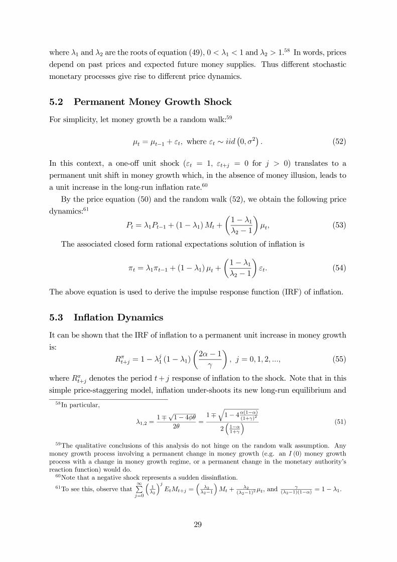
For simplicity, let money growth be a random walk:59

µt = µt−1 + εt, where εt ∼ iid¡0, σ2

¢. (52)

In this context, a one-off unit shock (εt = 1, εt+j = 0 for j > 0) translates to a

permanent unit shift in money growth which, in the absence of money illusion, leads to

a unit increase in the long-run inflation rate.60

By the price equation (50) and the random walk (52), we obtain the following price

dynamics:61

Pt = λ1Pt−1 + (1− λ1)Mt +

µ1− λ1λ2 − 1

¶µt, (53)

The associated closed form rational expectations solution of inflation is

πt = λ1πt−1 + (1− λ1)µt +

µ1− λ1λ2 − 1

¶εt. (54)

The above equation is used to derive the impulse response function (IRF) of inflation.

5.3 Inflation Dynamics

It can be shown that the IRF of inflation to a permanent unit increase in money growth

is:

Rπt+j = 1− λj1 (1− λ1)

µ2α− 1

γ

¶, j = 0, 1, 2, ..., (55)

where Rπt+j denotes the period t+ j response of inflation to the shock. Note that in this

simple price-staggering model, inflation under-shoots its new long-run equilibrium and

58In particular,

λ1,2 =1∓√1− 4φθ2θ

=1∓

q1− 4α(1−α)

(1+γ)2

2³1−α1+γ

´ (51)

59The qualitative conclusions of this analysis do not hinge on the random walk assumption. Anymoney growth process involving a permanent change in money growth (e.g. an I (0) money growthprocess with a change in money growth regime, or a permanent change in the monetary authority’sreaction function) would do.60Note that a negative shock represents a sudden dissinflation.61To see this, observe that

∞Pj=0

³1λ2

´jEtMt+j =

³λ2

λ2−1

´Mt +

λ2(λ2−1)2µt, and

γ(λ2−1)(1−α) = 1− λ1.

29

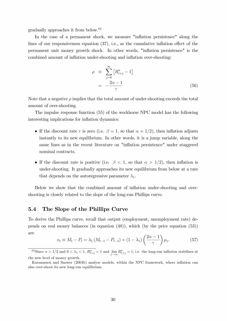
gradually approaches it from below.62

In the case of a permanent shock, we measure "inflation persistence" along the

lines of our responsiveness equation (37), i.e., as the cumulative inflation effect of the

permanent unit money growth shock. In other words, "inflation persistence" is the

combined amount of inflation under-shooting and inflation over-shooting:

ρ ≡∞Xj=0

£Rπt+j − 1

¤= −2α− 1

γ(56)

Note that a negative ρ implies that the total amount of under-shooting exceeds the total

amount of over-shooting.

The impulse response function (55) of the workhorse NPC model has the following

interesting implications for inflation dynamics:

• If the discount rate r is zero (i.e. β = 1, so that α = 1/2), then inflation adjustsinstantly to its new equilibrium. In other words, it is a jump variable, along the

same lines as in the recent literature on "inflation persistence" under staggered

nominal contracts.

• If the discount rate is positive (i.e. β < 1, so that α > 1/2), then inflation is

under-shooting. It gradually approaches its new equilibrium from below at a rate

that depends on the autoregressive parameter λ1.

Below we show that the combined amount of inflation under-shooting and over-

shooting is closely related to the slope of the long-run Phillips curve.

5.4 The Slope of the Phillips Curve

To derive the Phillips curve, recall that output (employment, unemployment rate) de-

pends on real money balances (in equation (48)), which (by the price equation (53))

are

xt ≡Mt − Pt = λ1 (Mt−1 − Pt−1) + (1− λ1)

µ2α− 1

γ

¶µt. (57)

62Since α > 1/2 and 0 < λ1 < 1, Rπt+j < 1 and lim

j→∞Rπt+j = 1, i.e. the long-run inflation stabilises at

the new level of money growth.Karanassou and Snower (2004b) analyse models, within the NPC framework, where inflation can

also over-shoot its new long-run equilibrium.

30

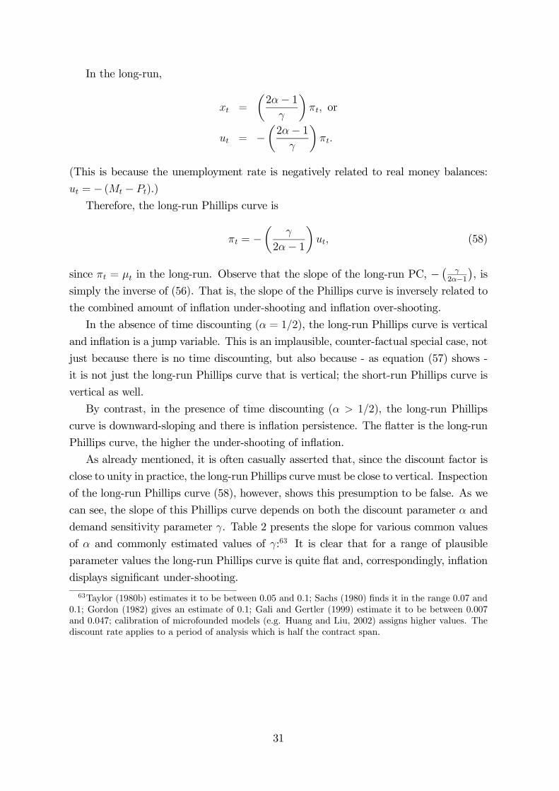
In the long-run,

xt =

µ2α− 1

γ

¶πt, or

ut = −µ2α− 1

γ

¶πt.

(This is because the unemployment rate is negatively related to real money balances:

ut = − (Mt − Pt).)

Therefore, the long-run Phillips curve is

πt = −µ

γ

2α− 1

¶ut, (58)

since πt = µt in the long-run. Observe that the slope of the long-run PC, −¡

γ2α−1

¢, is

simply the inverse of (56). That is, the slope of the Phillips curve is inversely related to

the combined amount of inflation under-shooting and inflation over-shooting.

In the absence of time discounting (α = 1/2), the long-run Phillips curve is vertical

and inflation is a jump variable. This is an implausible, counter-factual special case, not

just because there is no time discounting, but also because - as equation (57) shows -

it is not just the long-run Phillips curve that is vertical; the short-run Phillips curve is

vertical as well.

By contrast, in the presence of time discounting (α > 1/2), the long-run Phillips

curve is downward-sloping and there is inflation persistence. The flatter is the long-run

Phillips curve, the higher the under-shooting of inflation.

As already mentioned, it is often casually asserted that, since the discount factor is

close to unity in practice, the long-run Phillips curve must be close to vertical. Inspection

of the long-run Phillips curve (58), however, shows this presumption to be false. As we

can see, the slope of this Phillips curve depends on both the discount parameter α and

demand sensitivity parameter γ. Table 2 presents the slope for various common values

of α and commonly estimated values of γ:63 It is clear that for a range of plausible

parameter values the long-run Phillips curve is quite flat and, correspondingly, inflation

displays significant under-shooting.

63Taylor (1980b) estimates it to be between 0.05 and 0.1; Sachs (1980) finds it in the range 0.07 and0.1; Gordon (1982) gives an estimate of 0.1; Gali and Gertler (1999) estimate it to be between 0.007and 0.047; calibration of microfounded models (e.g. Huang and Liu, 2002) assigns higher values. Thediscount rate applies to a period of analysis which is half the contract span.

31

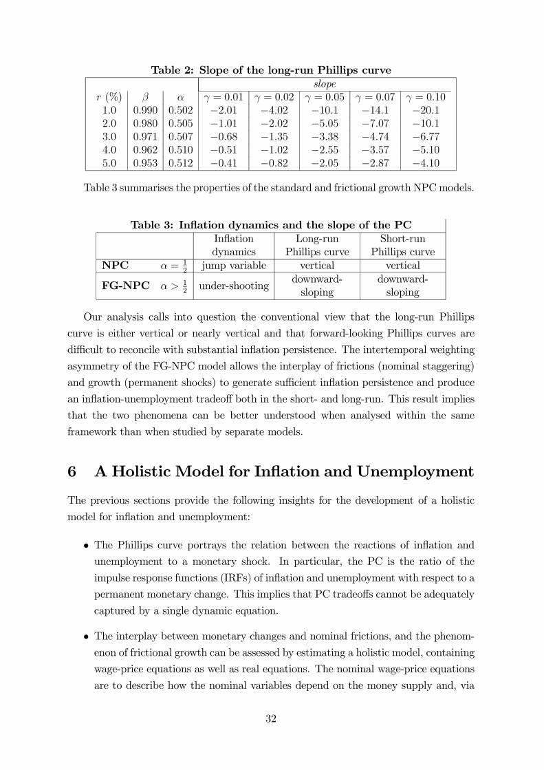
Table 2: Slope of the long-run Phillips curveslope

r (%) β α γ = 0.01 γ = 0.02 γ = 0.05 γ = 0.07 γ = 0.101.0 0.990 0.502 −2.01 −4.02 −10.1 −14.1 −20.12.0 0.980 0.505 −1.01 −2.02 −5.05 −7.07 −10.13.0 0.971 0.507 −0.68 −1.35 −3.38 −4.74 −6.774.0 0.962 0.510 −0.51 −1.02 −2.55 −3.57 −5.105.0 0.953 0.512 −0.41 −0.82 −2.05 −2.87 −4.10

Table 3 summarises the properties of the standard and frictional growth NPCmodels.

Table 3: Inflation dynamics and the slope of the PCInflationdynamics

Long-runPhillips curve

Short-runPhillips curve

NPC α = 12

jump variable vertical vertical

FG-NPC α > 12under-shooting

downward-sloping

downward-sloping

Our analysis calls into question the conventional view that the long-run Phillips

curve is either vertical or nearly vertical and that forward-looking Phillips curves are

difficult to reconcile with substantial inflation persistence. The intertemporal weighting

asymmetry of the FG-NPC model allows the interplay of frictions (nominal staggering)

and growth (permanent shocks) to generate sufficient inflation persistence and produce

an inflation-unemployment tradeoff both in the short- and long-run. This result implies

that the two phenomena can be better understood when analysed within the same

framework than when studied by separate models.

6 A Holistic Model for Inflation and Unemployment

The previous sections provide the following insights for the development of a holistic

model for inflation and unemployment:

• The Phillips curve portrays the relation between the reactions of inflation andunemployment to a monetary shock. In particular, the PC is the ratio of the

impulse response functions (IRFs) of inflation and unemployment with respect to a

permanent monetary change. This implies that PC tradeoffs cannot be adequately

captured by a single dynamic equation.

• The interplay between monetary changes and nominal frictions, and the phenom-enon of frictional growth can be assessed by estimating a holistic model, containing

wage-price equations as well as real equations. The nominal wage-price equations

are to describe how the nominal variables depend on the money supply and, via

32

the nominal frictions, on the past and future nominal variables. Then, in the

presence of frictional growth, money growth shocks lead to changes in the rela-

tive magnitudes of nominal variables, such as changes in real money balances or

changes in the real wage. On this basis, the real equations are to describe how

real variables, such as unemployment, respond to these changes in the relations

among nominal variables.

• The relation of wages and prices to their past and expected future values may beexpressed in terms of nominal equations that are backward-looking. The reason, as

shown above, is that when the rational expectations solution of the price equation

is derived, the expected future values of nominal variables can be expressed in

terms of current and past endogenous variables.

To illustrate our holistic approach, we consider the model estimated by Karanassou,

Sala, and Snower (2005) for the US over the 1963-2000 period. This interactive dynamics

model consists of three equations - unemployment rate, price level, and nominal wage

- and contains no money illusion, no permanent nominal rigidities, and no departure

from rational expectations. We briefly describe the model below:

1. The unemployment rate is a function of its lags, real money balances, investment,

trade deficit, oil price, financial wealth, and social security contributions.

2. The price level depends on its lagged values, money supply, wages, unemployment

rate, productivity, oil price, and indirect taxes.

3. The nominal wage depends on its lags, price level, money supply, unemployment

rate, productivity, and benefits.

The wage and price setting equations portray nominal sluggishness (so that changes

in money growth lead to changes in real money balances), and the unemployment equa-

tion indicates how the changes in real money balances affect the unemployment rate.

Figure 2 shows that the model tracks the data very well.

.03

.04

.05

.06

.07

.08

.09

.10

.11

1970 1975 1980 1985 1990 1995 2000

ActualFitted

a. Unemployment rate

.01

.02

.03

.04

.05

.06

.07

.08

.09

.10

1970 1975 1980 1985 1990 1995 2000

ActualFitted

b. Inflation

5.6

5.7

5.8

5.9

6.0

1970 1975 1980 1985 1990 1995 2000

Actual Fitted

c. Real wage

Figure 2. Actual and fitted values.

33

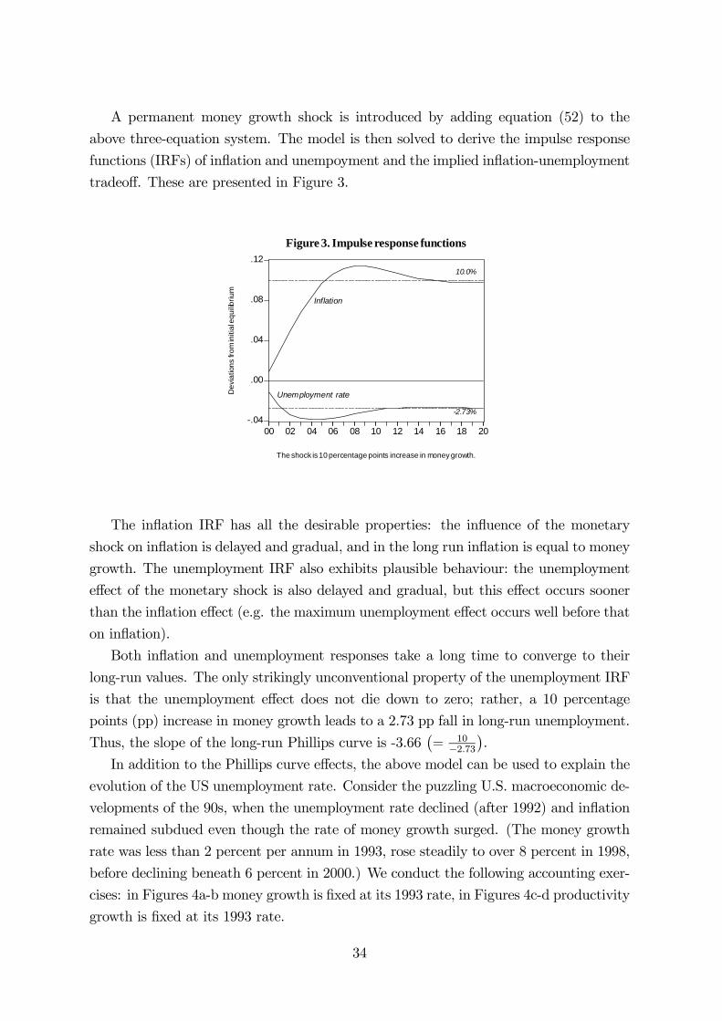
A permanent money growth shock is introduced by adding equation (52) to the

above three-equation system. The model is then solved to derive the impulse response

functions (IRFs) of inflation and unempoyment and the implied inflation-unemployment

tradeoff. These are presented in Figure 3.

-.04

.00

.04

.08

.12

00 02 04 06 08 10 12 14 16 18 20

Figure 3. Impulse response functions

Inflation

Unemployment rate

10.0%

-2.73%

Dev

iatio

ns fr

om in

itial

equ

ilibriu

m

The shock is 10 percentage points increase in money growth.

The inflation IRF has all the desirable properties: the influence of the monetary

shock on inflation is delayed and gradual, and in the long run inflation is equal to money

growth. The unemployment IRF also exhibits plausible behaviour: the unemployment

effect of the monetary shock is also delayed and gradual, but this effect occurs sooner

than the inflation effect (e.g. the maximum unemployment effect occurs well before that

on inflation).

Both inflation and unemployment responses take a long time to converge to their

long-run values. The only strikingly unconventional property of the unemployment IRF

is that the unemployment effect does not die down to zero; rather, a 10 percentage

points (pp) increase in money growth leads to a 2.73 pp fall in long-run unemployment.

Thus, the slope of the long-run Phillips curve is -3.66¡= 10

−2.73¢.

In addition to the Phillips curve effects, the above model can be used to explain the

evolution of the US unemployment rate. Consider the puzzling U.S. macroeconomic de-

velopments of the 90s, when the unemployment rate declined (after 1992) and inflation

remained subdued even though the rate of money growth surged. (The money growth

rate was less than 2 percent per annum in 1993, rose steadily to over 8 percent in 1998,

before declining beneath 6 percent in 2000.) We conduct the following accounting exer-

cises: in Figures 4a-b money growth is fixed at its 1993 rate, in Figures 4c-d productivity

growth is fixed at its 1993 rate.

34

.040

.044

.048

.052

.056

.060

.064

.068

.072

1993 1994 1995 1996 1997 1998 1999 2000

a. Money growth and unemployment

Actual unemployment

Simulated unemployment(money growth constantat its 1993 rate)

-.03

-.02

-.01

.00

.01

.02

.03

1993 1994 1995 1996 1997 1998 1999 2000

b. Money growth and inflation

Actual inflation

S imulated inflation(money growth constantat i ts 1993 rate)

.040

.044

.048

.052

.056

.060

.064

.068

.072

1993 1994 1995 1996 1997 1998 1999 2000

c. Productivity growth and unemployment

Actual unemployment

Simulated unemployment(prod. growth constantat its 1993 rate)

.012

.016

.020

.024

.028

.032

.036

.040

.044

1993 1994 1995 1996 1997 1998 1999 2000

d. Productivity growth and inflation

Actualinflation

Simulated inflation(productivity growth constantat its 1993 rate)

Figure 4

First, the surge of money growth over the second half of the 90s can account for over

a half of the decline in unemployment over this period (Figure 4a). Second, the money

growth surge was of course associated with a rise in inflation (Figure 4b). But, third, this

inflationary influence was substantially undone by the fall in inflation associated with the

increase in productivity growth over the period (Figure 4d). Finally, the contribution of

productivity growth to the fall in unemployment is modest: around 20% of the overall

decrease in unemployment over the period (Figure 4c).

The above interactive dynamics framework can be expanded by endogenising more

real variables (e.g. productivity), and the analysis can be extended to include the

influence of other variables (e.g. trade deficit, budget deficit) on both inflation and

unemployment.

35

7 Conclusions

The orthodox view that there is no long-run relationship between inflation and unem-

ployment has implied that the evolution of inflation and unemployment can be ade-

quately modeled by separate economic branches. These branches comply with a vertical

PC and the existence of a natural rate of unemployment.

In particular, the inflation dynamics macro branch takes for granted the existence

of the NRU and estimates the unemployment rate compatible with inflation stability -

the NAIRU. The labour macro branch takes for granted the existence of the NAIRU,

and tries to identify the real economic forces that drive the NRU.

So speaking, the conventional inflation dynamics and unemployment rate models can

be viewed as the two sides of the same coin - the coin of the classical dichotomy.

In this paper we overviewed the literature of the Phillips curve and critically assessed

the restrictions that need to be imposed so that its models predict a zero inflation-

unemployment tradeoff, at least in the long-run.

We showed that the orthodox view that the long-run NPC is either vertical or nearly

vertical and that forward-looking Phillips curves are difficult to reconcile with substan-

tial inflation persistence relies on the implausible assumption of intertemporal weighting

symmetry (symmetric backward- and forward-looking elements in the price-setting be-

haviour due to no time discounting).

We then demonstrated that when intertemporal weighting asymmetry is introduced

in the NPC, the resulting model allows the interplay of frictions (nominal staggering)

and growth (permanent shocks) to generate sufficient inflation persistence and produce

an inflation-unemployment tradeoff in both the short- and long-runs. We call this model

the frictional growth NPC and, like the standard NPC, it contains no money illusion,

no permanent nominal rigidities, and no departure from rational expectations.

We also discussed the traditional dynamics (single equation) and interactive dynam-

ics (multi-equation) unemployment rate models and argued in favour of an interactive

dynamics labour market model.

Our analysis calls for the adoption of a holistic framework that can jointly model

inflation dynamics, estimate the inflation-unemployment tradeoff, and determine the

factors responsible for the movements of the long-run equilibrium unemployment rate.

We argue that an interactive dynamics model that includes wage-price setting equa-

tions and labour market ones can jointly evaluate Phillips curve effects and identify

the temporary and permanent shocks that give rise to the observed unemployment rate

trajectory.

36

References

[1] Ahmed, S., and J. H. Rogers (2000): “Inflation and the great ratios: Long-term evidencefrom the U.S.,” Journal of Monetary Economics, 45, 3-35.

[2] Akerlof, G.A., W.T. Dickens, and G. L. Perry (1996): “The Macroeconomics of LowInflation,” Brookings Papers on Economic Activity, 1:1996, pp. 1—76.

[3] Akerlof, G.A., W.T. Dickens, and G. L. Perry (2000): “Near-Rational Wage and Price Set-ting and the Long-Run Phillips Curve,” Brookings Papers on Economic Activity, 1:2000,pp. 1—60.

[4] Ascari, G. (1998): “Superneutrality of money in staggered wage-setting models,” Macro-economic Dynamics, no 2, pp. 383-400.

[5] Ascari, G. (2000): “Optimising agents, staggered wages and persistence in the real effectsof monetary shocks,” The Economic Journal, 110, July, pp. 664-686.

[6] Ball, L. (1997): “Disinflation and the NAIRU,” in C.D. Romer and D.H. Romer (eds.),Reducing Inflation: Motivation and Strategy, Chicago: University of Chicago Press, pp.167-194.

[7] Ball, L. (1999): “Aggregate demand and long-run unemployment,” Brooking Papers onEconomic Activity, 2:1999, pp. 189-251.

[8] Bande, R., and M. Karanassou (2006): “Labour Market Flexibility and Regional Unem-ployment Rate Dynamics: Spain 1980-1995”, mimeo.

[9] Blanchard, O. (2000): “The Economics of Unemployment: shocks, Institutions and In-teractions,” Lionel Robins Lectures.

[10] Blanchard, O. (2005): “Monetary Policy and Unemployment,” in Monetary Policy andUnemployment - US, Euro-Area, and Japan, W. Semmler (ed.), Routledge, London.

[11] Bårdsen, G., E. Jansen, and R. Nymoen (2002), “The Empirical (Ir)relevance of the NewKeynesian Phillips Curve,” Norwegian University of Science and Technology, WorkingPaper Series No. 21/2002.

[12] Bårdsen, G., E. Jansen, and R. Nymoen (2004), “Econometric Evaluation of the NewKeynesian Phillips Curve,” Oxford Bulletin of Economics and Statistics, 66, 671-686.

[13] Bernanke, B. and I. Mihov (1998): “The Liquidity Effect and Long-Run Neutrality,”Carnegie-Rochester Conference Series on PublicPolicy, vol. 49, 1, pp. 149-94.

[14] Bullard, J., and J. W. Keating (1995): “The long-run relationship between inflation andoutput in postwar economies,” Journal of Monetary Economics, 36, pp. 477-496.

[15] Calvo, G. A. (1983): “Staggered Prices in a Utility-Maximizing Framework,” Journal ofMonetary Economics, 12(3), 383-398.

[16] Campbell, J. and G.N. Mankiw (1987): “Are Output Fluctuations Transitory?,” Quar-terly Journal of Economics, pp. 857-880.

37

[17] Coakley, J., A. M. Fuertes, and G. Zoega (2001): “Evaluating the Persistence and Struc-turalist Theories of Unemployment,” Studies in Nonlinear Dynamics and Econometrics,5 (3), pp. 179-202.

[18] Clarida, R., J. Galí and M. Gertler (1999): “The science of monetary policy: A NewKeynesian perspective,” Journal of Economic Literature, 37, December, pp. 1661-1707.

[19] Dolado, J.J., J.D. López-Salido and J.L. Vega (2000): “Unemployment and inflationpersistence in Spain: Are there Phillips tradeoffs?” Spanish Economic Review, 2, pp.267-291.

[20] Fair, R.C. (2000): “Testing the NAIRU Model for the United States,” The Review ofEconomics and Statistics, pp. 64-71.

[21] Fisher, M.E. and J.J. Seater (1993): “Long-run neutrality and supeneutrality in anARIMA framework,” American Economic Review, 83, pp. 402-415.

[22] Fitoussi, J.P., D. Jestaz, E.S. Phelps and G. Zoega (2000): “Roots of Recent Recoveries:Labor Reforms or Private sector Forces,” Brooking Papers on Economic Activity, 1:2000,pp. 292-304.

[23] Fuhrer, J. C. and G. Moore: (1995): “Inflation Persistence,” The Quarterly Journal ofEconomics, CX, pp. 127—160.

[24] Fuhrer, J. C. (1997): “The (Un)Importance of Forward-Looking Behavior in Price Spec-ifications,” Journal of Money, Credit, and Banking, 29 (3), pp.338-350.

[25] Galí, J. (2003): “New Perspectives on Monetary Policy, Inflation, and the Business Cycle,”in Advances in Economic Theory, M. Dewatripont, L. Hansen, and S.T. Turnovsky (eds),vol. III, Cambridge University Press, pp. 151-197.

[26] Galí, J. and M. Gertler (1999): “Inflation dynamics: a structural econometric analysis,”Journal of Monetary Economics, 44, pp. 195-222.

[27] Galí, J., M. Gertler and J.D. López-Salido (2001): “European inflation dynamics,” Euro-pean Economic review, 45, pp. 1237-1270.

[28] Goodfriend, M. and R.G. King (1997): “The new neoclassical synthesis and the role ofmonetary policy,” NBER Macroeconomics Annual, pp. 231-295.

[29] Gordon, R. J. (1982): Price Inertia and Policy ineffectiveness in the United States, 1890-1980. Journal of Political Economy, 90(6), 1087-1117.

[30] Gordon, R. J. (1983): “A century of evidence on wage and price stickiness in the UnitedStates, the United Kingdom, and Japan” in Macroeconomics, prices, and quantities, J.Tobin (Ed.), Washington, D.C.: Brookings Institution, pp. 85-121.

[31] Gordon, R.J. (1990): “What is New-Keynesian Economics?” Journal of Economic Liter-ature, vol. 28, 3, september, pp. 1115-1171.

[32] Gordon, R.J. (1997a): “The Time-Varying NAIRU and Its Implications for EconomicPolicy,” Journal of Economic Perspectives, vol. 11, 1, pp. 11-32.

38

[33] Gordon, R.J. (1997b): “Is there a trade-off between unemployment and productivitygrowth,” in D.J. Snower and G. de la Dehesa (eds), Unemployment Policy: GovernmentOptions for the Labour Market, CU Press, Cambridge.

[34] Gordon, R.J. (1998): “Foundations of the Goldilocks economy: supply shocks and theTime-Varying NAIRU,” Brooking Papers on Economic Activity, 2: 1998, pp. 297-346.

[35] Graham, L. and D.J. Snower (2002): “The return of the long-run Phillips curve,” CEPRDiscussion Paper 3691, Centre for Economic Policy Research, London; IZA DiscussionPaper 646, Institute for the Study of Labor, Bonn.

[36] Graham, L. and D.J. Snower (2004): “The real effects of money growth in dynamicequilibrium,” ECB Working Paper, no 412, European Central Bank, Frankfurt.

[37] Grier, K. B., and M. J. Perry (1998): “On Inflation and Inflation Uncertainty in the G7countries,” Journal of International Money and Finance, 17, pp. 671-689.

[38] Helpman, E. and L. Leiderman (1990): “Real wages, monetary accommodation, andinflation,” European Economic Review, 34, pp. 897-911.

[39] Henry, S.G.B., M. Karanassou and D.J. Snower (2000): “Adjustment Dynamics and theNatural Rate,” Oxford Economic Papers, 52, pp. 178-203.

[40] Huang, K.X.D. and Z. Liu (2002): “Staggered price-setting, staggered wage-setting andbusiness cycle persistence,” Journal of Monetary Economics, 49, pp. 405-433.

[41] Karanassou, M. and D.J. Snower (1997): “Is the natural rate a reference point?,” Euro-pean Economic Review, 41, pp. 559-569.

[42] Karanassou, M. and D. J. Snower (1996), “Explaining Disparities in Unemployment Dy-namics” in Baldassari M., L. Paganetto, and E.S. Phelps (eds), The 1990’s Slump: Causesand Cures, Macmillan Press and Rivista di Politica Economica.

[43] Karanassou, M. and D.J. Snower (1998): “How Labor Market Flexibility Affects Un-employment: Long-Term Implications of the Chain Reaction Theory,” The EconomicJournal, 108, May, pp. 832-849.

[44] Karanassou, M. and D.J. Snower (2004a): ”Unemployment Invariance ”, German Eco-nomic Review, 5(3), 297-317.

[45] Karanassou, M. and D.J. Snower (2004b): “Inflation Persistence Revisited,” Queen MaryWorking Paper, 518, University of London, London.

[46] Karanassou, M., H. Sala and D.J. Snower (2002): “Long-run inflation-unemploymentdynamics: The Spanish Phillips curve and economic policy,” IZA Discussion Paper, 645,IZA, Bonn.

[47] Karanassou, M., H. Sala and D.J. Snower (2003a): “Unemployment in the EuropeanUnion: A Dynamic Reappraisal,” Economic Modelling, 20, pp. 237-273.

[48] Karanassou, M., H. Sala and D.J. Snower (2003b): “The European Phillips curve: Doesthe NAIRU exist?” Applied Economics Quarterly, vol. 49, 2, pp. 93-121.

39

[49] Karanassou, M., H. Sala and D.J. Snower (2004): “Unemployment in the EuropeanUnion: Institutions, Prices and Growth,” CESifo Working Paper Series, 1247, Munich.

[50] Karanassou, M., H. Sala and D.J. Snower (2005): “A Reappraisal of the Inflation-Unemployment tradeoff,” European Journal of Political Economy, vol. 21, 1, pp. 1-32.

[51] King, R.G. and M.W. Watson (1994): “The post-war U.S. Phillips curve: a revisionisteconometric history,” Carnegie-Rochester Conference Series on Public Policy, 41, pp.157-219.

[52] Layard, R., S. Nickell, and R. Jackman (1991), Unemployment: Macroeconomic Perfor-mance and the Labour Market, Oxford: Oxford University Press.

[53] Malley, J., and T. Moutos (2001): “Capital Accumulation and Unemployment: A Taleof Two Continents,” Scandinavian Journal of Economics, 103 (1), pp. 79-99.

[54] Mankiw, N.G. (2001): “The inexorable and mysterious tradeoff between inflation andunemployment,” The Economic Journal, 111, pp. C45-C61.

[55] Mankiw, N.G. and R. Reis (2002): “Sticky information versus sticky prices: a proposal toreplace the New Keynesian Phillips curve,” The Quarterly Journal of Economics, 117(4),pp. 1295-1328.

[56] Modigliani, F. (2000): “Europe’s economic problems,” Prepared for testimony before theMonetary Committee of the European Parliament.

[57] Modigliani, F. and L. Papademos (1976): “Monetary policy for the coming quarters: Theconflicting views,” The New England Economic Review, 1976, pp. 2-35. Reprinted in TheCollected Papers of Franco Modigliani (1980), 3, pp. 186-219, MIT Press: CambridgeMass.

[58] Phelps, E. S. (1978), Disinflation without Recession: Adaptive Guideposts and MonetaryPolicy, Weltwirtschaftliches Archiv, C, 239-265.

[59] Phelps, E. S. (1994): Structural Booms: The Modern Equilibrium Theory of Unemploy-ment, Interest and Assets, Harvard University Press, Cambridge (MA).

[60] Phelps, E.S. (1999): “Behind this structural boom: the role of asset valuations,” TheAmerican Economic Review, Papers and Proceedings, vol. 89, 2, May, pp. 63-68.

[61] Phelps, E. and G. Zoega (1996): “Do the main structural forces of the 1970s and 1980saccount for the 90s slump as well?,” in M. Baldassari, L. Paganetto and E. S. Phelps(eds), The 90s Slump: Causes and Cures, MacMillan Press, London.

[62] Phelps, E. and G. Zoega (1997): “The rise and downward trend of the natural rate,”American Economic Review Papers and Proceedings, pp. 283-289.

[63] Phelps, E. and G. Zoega (1998): “Natural rate theory and OECD unemployment,” TheEconomic Journal, vol. 108, pp. 782-801.

[64] Phelps, E. and G. Zoega (2001): “Structural booms: productivity expectations and assetvaluations,” Economic Policy, 32, April, pp. 85-126.

40

[65] Pivetta, F., and R. Reis (2004): “The Persistence of Inflation in the United States,”manuscript, Harvard University.

[66] Roberts, J.M. (1995): “New Keynesian Economics and the Phillips curve,” Journal ofMoney, Credit and Banking, 27 (4,1), 975-984.

[67] Rotemberg, J. (1982), “Monopolistic Price Adjustment and Aggregate Output,” Reviewof Economic Studies, 44, 517-531.

[68] Rowthorn, R. (1999), “Unemployment,wage bargaining and capital-labour substitution,”Cambridge Journal of Economics, 23, 413-425.

[69] Rudd, J. and K. Whelan (2005): “New Tests of the New-Keynesian Phillips Curve,”Journal of Monetary Economics, 52 (6), 1167-1181.

[70] Rudebusch, G. D. and L.E.O. Svensson (1999): “Policy rules for inflation targeting,” inMonetary Policy Rules, edited by J.B. Taylor, The University of Chicago Press, 203-246.

[71] Sachs, J. (1980): “The changing cyclical behavior of wages and prices: 1890-1976,” Amer-ican Economic Review, 70, 78-90.

[72] Staiger, D., J.H. Stock and M. Watson (1997a): “How Precise are Estimates of theNatural Rate of Unemployment,” in C. Romer and D. Romer (eds.), Reducing Inflation:Motivation and Strategy, University of Chicago Press.

[73] Staiger, D., J.H. Stock and M. Watson (1997b): “The NAIRU, Unemployment and Mon-etary Policy,” Journal of Economic Perspectives, vol. 11, no 1, pp. 33-49.

[74] Svensson, L.E.O. (2000): “Open economy inflation targeting,” Journal of InternationalEconomics, 50, pp. 155-183.

[75] Taylor, J.B. (1979), “Staggered Wage Setting in a Macro Model,” American EconomicReview, No. 69, May, pp. 108-113.

[76] Taylor, J.B. (1980a): “Aggregate Dynamics and Staggered Contracts,” Journal of Polit-ical Economy, Vol. 88 (1), February, pp. 1-23.

[77] Taylor, J. B. (1980b), “Output and Price Stability: An International Comparison,” Jour-nal of Economic Dynamics and Control, 2, 109-132.

[78] Tobin, J. (1998): “Supply constraints on employment and output: NAIRU versus naturalrate,” International Conference in Memory of Fausto Vicarelli, Rome, Nov 21-23.

41