Phillips Curve Inflation Forecasts

James H. Stock Department of Economics, Harvard University and the National Bureau of Economic Research

and

Mark W. Watson*

Woodrow Wilson School and Department of Economics, Princeton University and the National Bureau of Economic Research

May 2008 (revised September 2008)

Abstract

This paper surveys the literature since 1993 on pseudo out-of-sample evaluation of inflation forecasts in the United States and conducts an extensive empirical analysis that recapitulates and clarifies this literature using a consistent data set and methodology. The literature review and empirical results are gloomy and indicate that Phillips curve forecasts (broadly interpreted as forecasts using an activity variable) are better than other multivariate forecasts, but their performance is episodic, sometimes better than and sometimes worse than a good (not naïve) univariate benchmark. We provide some preliminary evidence characterizing successful forecasting episodes. Key words: Inflation forecasting, time-varying parameters JEL codes: C53, E37 *Prepared for the Federal Reserve Bank of Boston Conference, “Understanding Inflation and the Implications for Monetary Policy: A Phillips Curve Retrospective,” June 9-11, 2008. We thank Ian Dew-Becker for research assistance and Michelle Barnes of the Boston Fed for data assistance. This research was funded in part by NSF grant SBR-0617811. Data and replication files are available at http://www.princeton.edu/~mwatson.

1. Introduction

Inflation is hard to forecast. There is now considerable evidence that Phillips

curve forecasts do not improve upon good univariate benchmark models. Yet the

backward-looking Phillips curve remains a workhorse of many macroeconomic

forecasting models and continues to be the best way to understand policy discussions

about the rates of unemployment and inflation.

After some preliminaries in Section 2, this paper begins in Section 3 by surveying

the past fifteen years of literature (since 1993) on inflation forecasting, focusing on

papers that conduct a pseudo out-of-sample forecast evaluation.1 A milestone in this

literature is Atkeson and Ohanian (2001), who consider a number of standard Phillips

curve forecasting models and show that none improve upon a four-quarter random walk

benchmark over the period 1984-1999. As we observe in this survey, Atkeson and

Ohanian (2001) deserve the credit for forcefully making this point, however their finding

has precursors dating back at least to 1994. The literature after Atkeson-Ohanian (2001)

finds that their specific result depends rather delicately on the sample period and the

forecast horizon. If, however, one uses other univariate benchmarks (in particular, the

unobserved components-stochastic volatility model of Stock and Watson (2007)), the

broader point of Atkeson-Ohanian (2001) – that, at least since 1985, Phillips curve

forecasts do not outperform univariate benchmarks on average – has been confirmed by

several studies. The development of this literature is illustrated empirically using six

prototype inflation forecasting models: three univariate models, Gordon’s (1990)

“triangle” model, an autoregressive-distributed lag model using the unemployment rate,

and a model using the term spread.

It is difficult to make comparisons across papers in this literature because the

papers use different sample periods, different inflation series, and different benchmark 1 Experience has shown that good in-sample fit of a forecasting model does not necessarily imply good out-of-sample performance. The method of pseudo out-of-sample forecast evaluation aims to address this by simulating the experience a forecaster would have using a forecasting model. In a pseudo out-of-sample forecasting exercise, one simulates standing at a given date t and performing all model specification and parameter estimation using only the data available at that date, then computing the h-period ahead forecast for date t+h; this is repeated for all dates in the forecast period.

1

models, and the quantitative results in the literature are curiously dependent upon these

details. In Section 4, we therefore undertake an empirical study that aims to unify and to

assess the results in the literature using quarterly U.S. data from 1953:I – 2008:I. This

study examines the pseudo out of sample performance of a total of 192 forecasting

procedures (157 distinct models and 35 combination forecasts), including the six

prototype models of Section 3, applied to forecasting five different inflation measures

(CPI-all, CPI-core, PCE-all, PCE-core, and the GDP deflator). This study confirms the

main qualitative results of the literature, although some specific results are found not to

be robust. Our study also suggests an interpretation of the strong dependence of

conclusions in this literature on the sample period. Specifically, one of our key findings

is that the performance of Phillips curve forecasts is episodic: there are times, such as the

late 1990s, when Phillips curve forecasts improved upon univariate forecasts, but there

are other times (such as the mid-1990s) when a forecaster would have been better off

using a univariate forecast. This provides a rather more nuanced interpretation of the

Atkeson-Ohanian (2001) conclusion concerning Phillips curve forecasts, one that is

consistent with the sensitivity of findings in the literature to the sample period.

A question that is both difficult and important is what this episodic performance

implies for an inflation forecaster today. On average, over the past fifteen years, it has

been very hard to beat the best univariate model using any multivariate inflation

forecasting model (Phillips curve or otherwise). But suppose you are told that next

quarter the economy would plunge into recession, with the unemployment rate jumping

by two percentage points. Would you change your inflation forecast? The literature is

now full of formal statistical evidence suggesting that this information should be ignored,

but we suspect that an applied forecaster would nevertheless reduce their forecast of

inflation over the one- to two-year horizon. In the final section, we suggest some reasons

why this might be justified.

2

2. Notation, Terminology, Families of Models, and Data

This section provides preliminary details concerning the empirical analysis and

gives the six prototype inflation forecasting models that will be used in Section 3 as a

guide to the literature. We begin by reviewing some forecasting terminology.

2.1 Terminology

h-period inflation. Inflation forecasting tends to focus on the one-year or two-

year horizons. We denote h-period inflation by htπ = 11

0

ht ii

h π−−−=∑ , where πt is the

quarterly rate of inflation at an annual rate, that is, πt = 400ln(Pt/Pt-1) (using the log

approximation), where Pt is the price index in quarter t. Four-quarter inflation at date t is 4tπ = 100ln(Pt/Pt-4), the log approximation to the percentage growth in prices over the

previous four quarters.

Direct and iterated forecasts. There are two ways to make an h-period ahead

model-based forecast. A direct forecast has ht hπ + as the dependent variable and t-dated

variables (variables observed at date t) as regressors, for example ht hπ + could be regressed

on htπ and the date-t unemployment rate (ut). At the end of the sample (date T), the

forecast of hT hπ + is computed “directly” using the estimated forecasting equation. In

contrast, an iterated forecast is based on a one-step ahead model, for example πt+1 could

be regressed on πt, which is then iterated forward to compute future conditional means of

πs, s > T+1, given data through time t. If predictors other than past πt are used then this

requires constructing a subsidiary model for the predictor, or alternatively modeling πt

and the predictor jointly (for example as VAR) and iterating the joint model forward.

Pseudo out-of-sample forecasts; rolling and recursive estimation. Pseudo out-

of-sample forecasting simulates the experience of a real-time forecaster by performing all

model specification and estimation using data through date t, making a h-step ahead

forecast for date t+h, then moving forward to date t+1 and repeating this through the

3

sample.2 Pseudo out-of-sample forecast evaluation captures model specification

uncertainty, model instability, and estimation uncertainty, in addition to the usual

uncertainty of future events.

Model estimation can either be rolling (using a moving data window of fixed size)

or recursive (using an increasing data window, always starting with the same

observation). In this paper, rolling estimation is based on a window of 10 years, and

recursive estimation starts in 1953:I or, for series starting after 1953:I, the earliest

possible quarter.

Root mean squared error and rolling RMSE. The root mean squared forecast

error (RMSE) of h-period ahead forecasts made over the period t1 to t2 is

1 2,t tRMSE = ( )2

1

2

|2 1

11

th ht h t h t

t tt tπ π+ +

=

−− + ∑ (1)

where |ht h tπ + is the pseudo out-of-sample forecast of h

t hπ + made using data through date t.

This paper uses rolling estimates of the RMSE, which are computed using a weighted

centered 15-quarter window:

rolling RMSE(t) = ( )7 72

|7 7

( ) (t t

h hs h s h s

s t s t

K s t K s tπ π+ +

+ += − = −

)− −∑ −∑

, (2)

where K is the biweight kernel, K(x) = (15/16)(1 – x2)21(|x|≤1).

2.2 Prototypical Inflation Forecasting Models

Single-equation inflation forecasting models can be grouped into four families:

(1) forecasts based solely on past inflation; (2) forecasts based on activity measures

(“Phillips curve forecasts”); (3) forecasts based on the forecasts of others; and (4)

2 A strict interpretation of pseudo out-of-sample forecasting would entail the use of real-time data (data of different vintages), but we interpret the term more generously to include the use of final data.

4

forecasts based on other predictors. This section lays out these families and provides

prototype examples of each.

(1) Forecasts based on past inflation. This family includes univariate time series

models such as ARIMA models and nonlinear or time-varying univariate models. We

also include in this family forecasts in which one or more inflation measure, other than

the series being forecasted, is used as a predictor; for example, past CPI core inflation or

past growth in wages could be used to forecast CPI-all inflation.

Three of our prototype models come from this family and serve as forecasting

benchmarks. The first is a direct autoregressive (AR) forecast, computed using the direct

autoregressive model,

ht hπ + – πt = μh + αh(L)Δπt + h

t hv + (AR(AIC)) (3)

where μh is a constant, αh(L) is a lag polynomial written in terms of the lag operator L,

is the h-step ahead error term (we will use v generically to denote regression error

terms), and the superscript h denotes the quantity for the h-step ahead direct regression.

In this prototype AR model, the lag length is determined by the Akaike Information

Criterion (AIC) over the range of 1 to 6 lags. This specification imposes a unit

autoregressive root.

ht hv +

The second prototype model is the Atkeson-Ohanian (2001) random walk model,

in which the forecast of the four-quarter rate of inflation, 44tπ + , is the average rate of

inflation over the previous four quarters, 4tπ (Atkeson and Ohanian only considered four-

quarter ahead forecasting). The Atkeson-Ohanian model thus is,

4

4tπ + = 4tπ + (AO). (4) 4

4tv +

The third prototype model is the Stock-Watson (2007) unobserved components-

stochastic volatility (UC-SV) model, in which πt has a stochastic trend τt, a serially

uncorrelated disturbance ηt, and stochastic volatility:

5

πt = τt + ηt, where ηt = ση,tζη,t (UC-SV) (5)

τt = τt–1 + εt, where εt = σε,tζε,t (6)

ln 2,tησ = ln 2

, 1tησ − + νη,t (7)

ln 2,tεσ = ln 2

, 1tεσ − + νε,t (8)

where ζt = (ζη,t, ζε,t) is i.i.d. N(0, I2), νt = (νη,t, νε,t) is i.i.d. N(0, γI2), and ζt and νt are

independently distributed, and γ is a scalar parameter. Although ηt and εt are

conditionally normal given ση,t and σε,t, unconditionally they are random mixtures of

normals and can have heavy tails. This is a one-step ahead model and forecasts are

iterated.

This model has only one parameter, γ, which controls the smoothness of the

stochastic volatility process. Throughout, we follow Stock and Watson (2007) and set γ

= 0.04.

(2) Phillips curve forecasts. We interpret Phillips curve forecasts broadly to

include forecasts produced using an activity variable, such as the unemployment rate, an

output gap, or output growth, perhaps in conjunction with other variables, to forecast

inflation or the change in inflation. This family includes both backwards-looking Phillips

curves and new Keynesian Phillips curves, although the latter appear infrequently (and

only recently) in the inflation forecasting literature.

We consider two prototype Phillips curve forecasts. The first is Gordon’s (1990)

“triangle model,” which in turn is essentially the model in Gordon (1982) with the minor

modifications.3 In the triangle model, inflation depends on lagged inflation, the

unemployment rate ut, and supply shock variables zt:

πt+1 = μ + αG(L)πt + β(L)ut+1 + γ(L)zt + vt+1. (triangle) (9)

3 The specification in Gordon (1990), which is used here, differs from Gordon (1982, Table 5, column 2) in three ways: (a) Gordon (1982) uses a polynomial distributed lag specification on lagged inflation, while Gordon (1990) uses the step function; (b) Gordon (1982) includes additional intercept shifts in 1970Q3-1975Q4 and 1976Q1-1980Q4, which are dropped in Gordon (1990); (c) Gordon (1982) uses Perry-weighted unemployment whereas here we use overall unemployment.

6

The prototype triangle model used here is that in Gordon (1990), in which (9) is specified

using the contemporaneous value plus four lags of ut (total civilian unemployment rate

ages 16+, seasonally adjusted), contemporaneous value plus four lags of the rate of

inflation of food and energy prices (computed as the difference between the inflation

rates in the deflator for “all-items” personal consumption expenditure (PCE) and the

deflator for PCE less food and energy), lags one through four of the relative price of

imports (computed as the difference of the rates of inflation of the GDP deflator for

imports and the overall GDP deflator), two dummy variables for the Nixon wage-price

control period, and 24 lags of inflation, where αG(L) imposes the step-function restriction

that the coefficients are equal within the groups of lags 1-4, 5-8, …, 21-24, and also that

the coefficients sum to one (a unit root is imposed).

Following Gordon (1998), multiperiod forecasts based on the triangle model (9)

are iterated using forecasted values of the predictors, where those forecasts are made

using subsidiary univariate AR(8) models of ut, food and energy inflation, and import

inflation.

The second prototype Phillips curve model is direct version of (9) without the

supply shock variables, specifically, the autoregressive distributed (ADL) lag model in

which forecasts are computed using the direct regression,

ht hπ + − πt = μh + αh(L)Δπt + βh(L)ut + h

t hv + , (ADL-u) (10)

where the degrees of αh(L) and βh(L) are chosen separately by AIC (maximum lag of 4),

and (like the triangle model) the ADL-u specification imposes a unit root in the

autoregressive dynamics for πt.

(3) Forecasts based on forecasts of others. The third family computes inflation

forecasts from explicit or implicit inflationary expectations or forecasts of others. These

forecasts include regressions based on implicit expectations derived from asset prices,

such as forecasts extracted from the term structure of nominal Treasury debt (which by

the Fisher relation should embody future inflation expectations) and forecasts extracted

from the TIPS yield curve. This family also includes forecasts based on explicit forecasts

7

of others, such as median forecasts from surveys such as the Survey of Professional

Forecasters.

Our prototypical example of forecasts in this family is a modification of the

Mishkin (1990) specification, in which the future change in inflation is predicted by a

matched-maturity spread between the interest rates on comparable government debt

instruments, with no lags of inflation. Here we consider direct four-quarter ahead

forecasts based on an ADL model using as a predictor the interest spread, spread1_90t,

between 1-year Treasury bonds and 90-day Treasury bills:

4

4tπ + − πt = μ + α(L)Δπt + β(L)spread1_90t + 44tv + . (ADL-spread) (11)

We emphasize that Mishkin’s (1990) regressions appropriately use term spread maturities

matched to the change in inflation being forecasted, which for (11) would be the change

in inflation over quarters t+2 to t+4, relative to t+1. (A matched maturity alternative to

spread1_90t in (11) would be the spread between 1-year Treasuries and the Fed Funds

rate, however those instruments have different risks.) Because the focus of this paper is

Phillips curve regressions we treat this regression simply as an example of this family and

provide references to recent studies of this family in Section 3.3.

(4) Forecasts based on other predictors. The fourth family consists of inflation

forecasts that are based on variables other than activity or expectations variables. An

example is a 1970s-vintage monetarist model in which M1 growth is used to forecast

inflation. Forecasts in this fourth family perform sufficiently poorly relative to the three

other approaches that they play negligible roles both in the literature and in current

practice, so to avoid distraction we do not track a model in this family as a running

example.

2.3 Data and transformations

The data set is quarterly for the United States from 1953:I – 2008:I. Monthly data

are converted to quarterly by computing the average value for the three months in the

quarter prior to any other transformations; for example quarterly CPI is the average of the

8

three monthly CPI values, and quarterly CPI inflation is the percentage growth (at an

annual rate, using the log approximation) of this quarterly CPI.

We examine forecasts of five measures of price inflation: the GDP deflator

(PGDP), the CPI for all items (CPI-all), CPI excluding food and energy (CPI-core), the

personal consumption expenditure deflator (PCE-all), and the personal consumption

expenditure deflator excluding food and energy (PCE-core).

In addition to the six prototype models, in Section 4 we consider forecasts made

using a total of 15 predictors, most of which are activity variables (GDP, industrial

production, housing starts, the capacity utilization rate, etc.). The full list of variables

and transformations is given in Appendix A.

Gap variables. Consistent with the pseudo out-of-sample forecasting philosophy,

the activity gaps used in the forecasting models in this paper are all one-sided. Following

Stock and Watson (2007), gaps are computed as the deviation of the series (for example,

log GDP) from a symmetric two-sided MA(80) approximation to the optimal lowpass

filter with pass band corresponding to periodicities of at least 60 quarters. The one-sided

gap at date t is computed by padding observations at dates s > t and s < 1 with iterated

forecasts and backcasts based on an AR(4), estimated recursively through date t.

3. An Illustrated Survey of the Literature on Phillips Curve

Forecasts, 1993-2008

This section surveys the literature during the past fifteen years (since 1993) on

inflation forecasting in the United States. The criterion for inclusion in this survey is

providing empirical evidence on inflation forecasts (model- and/or survey-based) in the

form of a true or pseudo out-of-sample forecast evaluation exercise. Such an evaluation

can use rolling or recursive forecasting methods based on final data; it can use rolling or

recursive methods using real-time data; or it can use forecasts actually produced and

recorded in real time such as survey forecasts. Most of the papers discussed here focus

on forecasting at horizons of policy relevance, one or two years. Primary interest is in

forecasting overall consumer price inflation (PCE, CPI), core inflation, or economy-wide

9

inflation (GDP deflator). There is little work on forecasting producer prices, although a

few papers consider producer prices as a predictor of headline inflation.

This survey also discusses some papers in related literatures, however we do not

attempt a comprehensive review of those related literatures. One such literature concerns

the large amount of interesting work that has been done on inflation forecasting in

countries other than the U.S.; see Rünstler (2002), Hubrich (2005), Canova (2007), and

Diron and Mojon (2008) for recent contributions and references. Another closely related

literature concerns in-sample statistical characterizations of changes in the univariate and

multivariate inflation process in the U.S. (e.g. Taylor (2000), Brainard and Perry (2000),

Cogley and Sargent (2002, 2005), Levin and Piger (2004), and Pivetta and Reis (2007))

and outside the U.S. (e.g. the papers associated with the European Central Bank Inflation

Persistence Network (2007)). There is in turn a literature that asks whether these changes

in the inflation process can be attributed, in a quantitative (in-sample) way, to changes in

monetary policy; papers in this vein include Estrella and Fuhrer (2003), Roberts (2004),

Sims and Zha (2004) and Primiceri (2006). A major theme of this survey is time-

variation in the Phillips curve from a forecasting perspective, most notably at the end of

the disinflation of the early 1980s but more subtly throughout the post-1984 period. This

time-variation is taken up in a great many papers (for example estimation of a time-

varying NAIRU and time variation in the slope of the Phillips curve), however those

papers are only discussed in passing unless they have a pseudo out-of-sample forecasting

component.

3.1 The 1990s: Warning Signs

The great inflation and disinflation of the 1970s and the 1980s was the formative

experience that dominated the minds and models of inflation forecasters through the

1980s and early 1990s, both because of the forecasting failures of 1960s-vintage (“non-

accelerationist”) Phillips curves and, more mechanically, because most of the variation in

the data comes from that period. The dominance of this episode is evident in Figure 1,

which plots the three measures of headline inflation (GDP, PCE-all, and CPI-all) from

1953Q1 to 2007Q4, along with the unemployment rate.

10

By the early 1980s, despite theoretical attacks on the backwards-looking Phillips

curve, Phillips curve forecasting specifications had coalesced around the Gordon (1982)

type triangle model (9) and variants. Figure 2 plots the rolling RMSE of the four-quarter

ahead pseudo out-of-sample forecast of CPI-all inflation, computed using (2), for the

recursively estimated AR(AIC) benchmark (3), the triangle model (9), and the ADL-u

model (10). As can be seen in Figure 2, these “accelerationist” Phillips curve

specifications (unlike their non-accelerationist ancestors) did in fact perform well during

the 1970s and 1980s.

The greatest success of the triangle model and the ADL-u model was forecasting

the fall in inflation during the early 1980s subsequent to the spike in the unemployment

rate in 1980, but in fact the triangle and ADL-u models improved upon the AR

benchmark nearly uniformly from 1965 through 1990. The main exception occurred

around 1986, when there was a temporary decline in oil prices. Figure 3 shows the four-

quarter ahead pseudo out-of-sample forecasts produced by the AR(AIC), triangle, and

ADL-u models are shown respectively in panels A-C of Figure 3. As can be seen in

Figure 3, the triangle model initially failed to forecast the decline in inflation in 1986,

then incorrectly predicted to last longer than it did. Interestingly, unlike the AR(AIC)

and ADL-u models, triangle model forecasts did not over-extrapolate the decline in

inflation in the early 1980s.

Stockton and Glassman (1987) documented the good performance of a triangle

model based on the Gordon (1982) specification of the triangle model over the 1977-

1984 period (they used the Council of Economic Advisors output gap instead of the

unemployment rate and a 16-quarter, not 24-quarter, polynomial distributed lag). They

reported a pseudo out-of-sample relative RMSE of the triangle model, relative to an

AR(4) model of the change in inflation, of 0.80 (eight quarter ahead iterated forecasts of

inflation measured by the Gross Domestic Business Product fixed-weight deflator)4.

Notably, Stockton and Glassman (1987) also emphasized that there seem to be few good

competitors to this model: a variety of monetarist models, including some that

incorporate expectations of money growth, all performed worse – in some cases, much

4 Stockton and Glassman (1987), Table 6, ratio of PHL(16,FE) to ARIMA RMSE for average of four intervals.

11

worse – than the AR(4) benchmark. This said, the gains from using a Phillips curve

forecast over the second half of the 1980s were slimmer than during the 1970s and early

1980s.

The earliest documentation of this relative deterioration of Phillips curve forecasts

of which we are aware is a little-known (2 Google Scholar cites) working paper by Jaditz

and Sayers (1994). They undertook a pseudo out-of-sample forecasting exercise of CPI-

all inflation using industrial production growth, the PPI, and the 90-day Treasury Bill rate

in a VAR and in a vector error correction model (VECM), with a forecast period of 1986-

1991 and a forecast horizon of one month. They reported a relative RMSE of .985 for the

VAR and a relative MSE in excess of one for the VECM, relative to an AR(1)

benchmark.

Cecchetti (1995) also provided early evidence of instability in Phillips curve

forecasts, although that instability was apparent only using in-sample break tests and did

not come through in his pseudo out-of-sample forecasting evaluation because of his

forecast sample period. He considered forecasts of CPI-all at horizons of 1-4 years based

on 18 predictors, entered separately, for two forecast periods, 1977-1994 (10 year rolling

window) and 1987-1994 (5 year rolling window). Inspection of Figure 2 indicates

Phillips curve forecasts did well on average over both of these windows, but that the

1987-1994 period was atypical of the post-1984 experience in that it is dominated by the

relatively good performance of Phillips curve forecasts during the 1990 recession.

Despite the good performance of Phillips curve forecasts over this period, using in-

sample break tests Cecchetti (1990) found multiple breaks in the relation between

inflation and (separately) unemployment, the employment/population ratio, and the

capacity utilization rate. He also found that good in-sample fit is essentially unrelated to

future forecasting performance.

Stock and Watson (1999) undertook a pseudo out-of-sample forecasting

assessment of CPI-all and PCE-all forecasts at the one-year horizon using (separately)

168 economic indicators, of which 85 were measures of real economic activity (industrial

production growth, unemployment, etc). They considered recursive forecasts computed

over two subsamples, 1970-1983 and 1984-1996. The split sample evidence indicated

major changes in the relative performance of predictors in the two subsamples, for

12

example the RMSE of the forecast based on the unemployment rate, relative to the AR

benchmark, was .89 in the 1970-1983 sample but 1.01 in the 1984-1996 sample. Using

in-sample test statistics, they also found structural breaks in the inflation – unemployment

relation, although interestingly these breaks were more detectable in the coefficients on

lagged inflation in the Phillips curve specifications than on the activity variables.

Cechetti, Chu and Steindel (2000) examined CPI inflation forecasts at the two-

year horizon using (separately) 19 predictors, including activity indicators. They

reported dynamic forecasts in which future values of the predictors are used to make

multi-period ahead forecasts (future employment is treated as known at the time the

forecast is made, so these are not psueduo out-of-sample). Notably, they found that over

this period the activity-based forecasts (unemployment, employment-population ratio,

and capacity utilization rate) typically underperformed the AR benchmark over this

period at the one-year horizon.

A final paper documenting poor Phillips curve forecasting performance,

contemporaneous with Atkeson-Ohanian (2001), is Camba-Mendezand and Rodriguez-

Palenzuela (2003; originally published as ECB working paper April 2001). They showed

that inflation forecasts at the one-year horizon based on realizable (that is, backwards-

looking) output gap measures, for the forecast period 1980 – 1999, underperform the AR

benchmark.

In short, during the 1990s a number of papers provided results that activity-based

inflation forecasts provided a smaller advantage relative to an AR benchmark since the

mid-1980s than they had before. Ambiguities remained, however, because this

conclusion seemed to depend on the sample period and specification, and in any event

one could find predictors which were exceptions in the sense that they appeared to

provide improvements in the later sample, even if their performance was lackluster in the

earlier sample.

3.2 Atkeson-Ohanian (2001)

Atkeson and Ohanian (2001) (AO) resolved the ambiguities in this literature of

the 1990s by introducing a new, simple univariate benchmark: the forecast of inflation

13

over the next four quarters is the value of four-quarter inflation today. AO showed that

this four-quarter random walk forecast improved substantially upon the AR benchmark

over 1984-1999. Figure 4 plots the moving RMSE of four-quarter ahead forecasts of

CPI-all inflation for three univariate forecasts: the AR(AIC) forecast (3), the AO forecast

(4), and the UC-SV forecast (5) - (8). Because the AO benchmark improved over the

1984-1999 period on the AR forecast, and because the AR forecast had more or less the

same performance as the unemployment-based Phillips curve on average over this period

(see Figure 2), it is not surprising that the AO forecast outperformed the Phillips curve

forecast over the 1984-1999 period. As AO dramatically showed, across 264

specifications (three inflation measures, CPI-all, CPI-core, and PCE-all, 2 predictors, the

unemployment rate and the CFNAI, and various lag specifications), the relative RMSEs

of a Phillips curve forecast to the AO benchmark ranged from 0.99 to 1.94: gains from

using a Phillips curve forecast were negligible at best, and some Phillips curve forecasts

went badly wrong. AO went one step further and demonstrated that, over the 1984-1999

period, Greenbook forecasts of inflation also underperformed their four-quarter random

walk forecast.

As Figures 2 and 4 demonstrate, one important source of the problem with

Phillips curve forecasts was their poor performance in the second half of the 1990s, a

period of strong, but at the time unmeasured, productivity growth that held down

inflation. The apparent quiescence of inflation in the face of strong economic growth

was puzzling at the time (for example, see Lown and Rich (1997)).

An initial response to the AO was to check whether their claims were accurate;

with a few caveats, by and large they were. Fisher, Liu, and Zhou (2002) used rolling

regressions with a 15-year window and showed that Phillips curve models outperformed

the AO benchmark in 1977-1984, and also showed that for some inflation measures and

some periods the Phillips curve forecasts outperform the AO benchmark post-1984 (for

example, Phillips curve forecasts improve upon AO forecasts of PCE-all over 1993-

2000). They also pointed out that Phillips curve forecasts based on the CFNAI achieve

60-70% accuracy in directional forecasting of the change of inflation, compared with

50% for the AO coin flip. Fisher, Liu, and Zhou (2002) suggested that Phillips curve

14

forecasts do relatively poorly in periods of low inflation volatility and after a regime

shift.

Stock and Watson (2003) extended the AO analysis to additional activity

predictors (as well as other predictors) and confirmed the dominance of the AO forecast

over 1985-1999 at the one-year horizon. Brave and Fisher (2004) extended the AO and

Fisher, Liu, and Zhou (2002) analyses by examining additional predictors and

combination forecasts. Their findings are broadly consistent with Fisher, Liu, and Zhou

(2002) in the sense that they found some individual and combination forecasts that

outperform AO over 1993-2000, although not over 1985-1992. Orphanides and van

Norden (2005) focused on Phillips curve forecasts using real-time gap measures, and they

concludeed that although ex-post gap Phillips curves fit well using in-sample statistics,

when real-time gaps and pseudo out-of-sample methods are used these too improve upon

the AR benchmark prior to 1983, but fail to do so over the 1984-2002 sample.

There are three notable recent studies that confirm the basic AO finding and

extend it, with qualifications. First, Stock and Watson (2007) focused on univariate

models of inflation and pointed out that the good performance of the AO random walk

forecast, relative to other univariate models, is specific to the four-quarter horizon and (as

can be seen by comparing the AO and UC-SV rolling RMSEs in Figure 4) to the AO

sample period. At any point in time, the UC-SV model implies an IMA(1,1) model for

inflation, with time-varying coefficients. The forecast function of this IMA(1,1) closely

matches the implicit AO forecast function over the 1984-1999 sample, however the

models diverge over other subsamples. Moreover, the rolling IMA(1,1) is in turn well

approximated by a ARMA(1,1) because the estimated AR coefficient is nearly one.5

Stock and Watson (2007) also reported some (limited) results for bivariate forecasts using

activity indicators (unemployment, one-sided gaps, and output growth) and confirmed the

5 The UC-SV model imposes a unit root in inflation so is consistent with the Pivetta-Reis (2007) evidence that the largest AR root in inflation has been essentially one throughout the postwar sample. But the time-varying relative variances of the permanent and transitory innovation allows for persistence to change over the course of the sample and for spectral measures of persistence to decline over the sample, consistent with Cogley and Sargent (2002, 2005).

15

AO finding that these Phillips curve forecast fail to improve systematically on the AO

benchmark or the UC-SV benchmark.

Second, Canova (2007) undertook a systematic evaluation of 4- and 8-quarter

ahead inflation forecasts for G7 countries using recursive forecasts over 1996-2000, using

a variety of activity variables (unemployment, employment, output gaps, GDP growth)

and other indicators (yield curve slope, money growth) as predictors. He found that, for

the U.S., bivariate direct regressions and trivariate VARs and BVARs did not improve

upon the univariate AO forecast. (Generally speaking, Canova (2007) also did not find

consistent improvements for multivariate models over univariate ones for the other G7

countries, and he reported evidence of instability of forecasts based on individual

predictors.) Canova (2007) also considered combination forecasts and forecasts

generated using a new Keynesian Phillips curve. Over the 1996-2000 sample, the

combination forecasts in the U.S. provided a small improvement over the AO forecast,

and the new Keynesian Phillips curve forecasts were never best and generally fared

poorly. In the case of the U.S., at least, these findings are not surprising in light of the

poor performance of Phillips curve forecasts during the low-inflation boom of the second

half of the 1990s.

Third, Ang, Bekaert, and Wei (2007) conducted a thorough assessment of

forecasts of CPI, CPI-core, CPI ex housing, and PCE inflation, using ten variants of

Phillips curve forecasts, 15 variants of term structure forecasts, combination forecasts,

and ARMA(1,1) and AR(1)-regime switching univariate models in addition to AR and

AO benchmarks. They too confirmed the basic AO message that Phillips curve models

fail to improve upon univariate models over forecast periods 1985-2002 and 1995-2002,

and their results constitute a careful summary of the current state of knowledge of

inflation forecasting models (both Phillips curve and term structure) in the U.S. One

finding in their study is that combination forecasts do not systematically improve on

individual indicator forecasts, a result that is puzzling in light of the success reported

elsewhere of combination forecasts (we return to this puzzle below). Ang, Bekaert, and

Wei (2007) also considered survey forecasts, and their most striking result is that survey

forecasts (the Michigan, Livingston, and Survey of Professional Forecasters surveys)

perform very well: for the inflation measures that the survey respondents are asked to

16

forecast, the survey forecasts nearly always beat the ARMA(1,1) benchmark, their best-

performing univariate model over the 1985-2002 period.6 Further study of rolling

regressions led them to suggest that the relatively good performance of the survey

forecasts might be due to the ability of professional forecasters to recognize structural

change more quickly than automated regression-based forecasts.7

An alternative forecast, so far unmentioned, is that inflation is constant. This

forecast works terribly over the full sample but Diron and Mojon (2008) found out that,

for PCE-core from 1995Q1-2007Q4, a forecast of a constant 2.0% inflation rate

outperforms AO and AR forecasts at the 8-quarter ahead horizon, although the AO

forecast is best at the 4-quarter horizon. They choose 2.0% as representative of an

implicit inflation target over this period, however because the U.S. does not have an

explicit ex-ante inflation target and this value was chosen retrospectively, this choice

does not constitute a psueduo out-of-sample forecast.

All these papers – from Jaditz and Sayers (1994) through Ang, Bekaert, and Wei

(2007) – point to time variation in the underlying inflation process and in Phillips curve

forecasting relations. Most of this evidence is based on changes in relative RMSEs, in

some cases augmented by Diebold-Mariano (1995) or West (1996) tests using asymptotic

critical values. As a logical matter, the apparent statistical significance of the changes in

the relative RMSEs between sample periods could be a spurious consequence of using a

poor approximation to the sampling distribution of the relevant statistics. Accordingly,

6 Koenig (2003, Table 3) presented in-sample evidence that real-time markups (nonfinancial corporate GDP divided by nonfinancial corporate employee compensation), in conjunction with the unemployment rate, significantly contribute to a forecast combination regression for 4-quarter CPI inflation over 1983-2001, however he did not present pseudo out-of-sample RMSEs. Two of Ang, Bekaert, and Wei’s (2007) models (their PC9 and PC10) include the output gap and the labor income share, specifications similar to the Koenig’s (2003), and the pseudo out-of-sample performance of these models is poor: over the two Ang, Bekaert, and Wei’s (2007) subsamples and four inflation measures, the RMSEs, relative to the ARMA(1,1) benchmark, range from 1.17 to 3.26. These results suggest that markups are not a solution to the poor performance of Phillips curve forecasts over the post-85 samples. 7 Cecchetti et. al. (2007, Section 7) provided in-sample evidence that survey inflation forecasts are correlated with future trend inflation, measured using the Stock-Watson (2007) UC-SV model. Thus a different explanation of why surveys perform well is that survey inflation expectations anticipate movements in trend inflation.

17

Clark and McCracken (2006) undertook a bootstrap evaluation of the relative RMSEs

produced using real-time output gap Phillips curves for forecasting the GDP deflator and

CPI-core. They reached the more cautious conclusion that much of the relatively poor

performance of forecasts using real-time gaps could simply be a statistical artifact that is

consistent with a stable Phillips curve, although they found evidence of instability in

coefficients on the output gap. One interpretation of the Clark-McCracken (2006)

finding is that, over the 1990-2003 period, there are only 14 nonoverlapping observations

on the four-quarter ahead forecast error, and estimates of ratios of variances with 14

observations inevitably have a great deal of sampling variability.

3.3 Attempts to Resuscitate Multivariate Inflation Forecasts, 1999 - 2007

One response to the AO findings has been to redouble efforts to find reliable

multivariate forecasting models for inflation. Some of these efforts used statistical tools,

including dynamic factor models, other methods for using a large number of predictors,

time-varying parameter multivariate models, and nonlinear time series models. Other

efforts exploited restrictions arising from economics, in particular from no-arbitrage

models of the term structure. Unfortunately, these efforts have failed to produce

substantial and sustained improvements over the AO or UC-SV univariate benchmarks.

Many-predictor forecasts I: dynamic factor models. The plethora of activity

indicators used in Philips curve forecasts indicates that there is no single, most natural

measure; in fact, these indicators can all be thought of as different ways to measure

underlying economic activity. This suggests modeling the activity variables jointly using

a dynamic factor model (Geweke (1977), Sargent-Sims (1977)), estimating the common

latent factor (underlying economic activity), and using that estimated factor as the

activity variable in Phillips curve forecasts. Accordingly, Stock and Watson (1999)

examined different activity measures as predictors of inflation, estimated (using principal

components, as justified by Stock and Watson (2002)) as the common factor among 85

monthly indicators of economic activity, and also as the first principal component of 165

series including the activity indicators plus other series. In addition to using information

in a very large number of series, Stock and Watson (2002) showed that principal

18

components estimation of factors can be robust to certain types of instability in a dynamic

factor model. Stock and Watson’s (1999) empirical results indicated that these estimated

factors registered improvements over the AR benchmark and over single-indicator

Phillips curve specifications in both 1970-1983 and 1984-1996 subsamples.

A version of the Stock-Watson (1999) common factor, computed as the principal

component of 85 monthly indicators of economic activity, has been published in real time

since January 2001 as the Chicago Fed National Activity Index (CFNAI) (Federal

Reserve Bank of Chicago, various). Hansen (2006) confirmed the main findings in Stock

and Watson (1999) about the predictive content of these estimated factors for inflation,

relative to a random walk forecast over a forecast period of 1960-2000.

Recent studies, however, have raised questions about the marginal value of

Phillips curve forecasts based on estimated factors, such as the CFNAI, for the post-1985

data. As discussed above, Atkeson and Ohanian showed that the AO forecast

outperformed CFNAI-based Phillips curves over the 1984-1999 period; this is consistent

with Stock and Watson’s (1999) findings because they used an AR benchmark. Banerjee

and Marcellino (2006) also found that Phillips curve forecasts using estimated factors

perform relatively poorly for CPI-all inflation over a 1991-2001 forecast period. On the

other hand, for the longer sample of 1983-2007, Gavin and Kliesen (2008) found that

recursive factor forecasts improve upon both the direct AR(12) (monthly data) and AO

benchmarks (relative RMSEs are between .88 and .95). In a finding that is inconsistent

with AO and with Figure 4, Gavin and Kliesen (2008) also found that the AR(12) model

outperforms AO at the 12-month horizon for three of the four inflation series; presumably

this surprising result is either a consequence of including earlier and later data than AO or

indicates some subtle differences between using quarterly data (as in AO and in Figure 4)

and monthly data.

Additional papers which use estimated factors to forecast inflation include

Watson (2003), Bernanke, Bovin, and Elias (2005), Boivin and Ng (2005, 2006),

D’Agostino and Giannone (2006), Giaccomini and White (2006). In an interesting meta-

analysis, Eichmeier and Ziegler (2006) considered a total of 46 studies of inflation and/or

output forecasts using estimated factors, including 19,819 relative RMSEs for inflation

forecasts in the U.S. and other countries. They concluded that factor model forecasts

19

tend to outperform small model forecasts in general, that the factor inflation forecasts

generally improve over univariate benchmarks at all horizons, and that rolling forecasts

generally outperform recursive forecasts. One difficulty with interpreting the Eichmeier-

Ziegler (2006) findings, however, is that their unit of analysis is a reported relative

RMSE, but the denominators (benchmark models) differ across studies; in the U.S. in

particular, it matters whether the AR or AO benchmark is used because their relative

performance changes over time.

Many-predictor forecasts II: Forecast combination, BMA, Bagging, and other

methods. Other statistical methods for using a large number of predictors are available

and have been tried for forecasting inflation. One approach is to use leading index

methods, in essence a model selection methodology. In the earliest high-dimensional

inflation forecasting exercise of which we are aware, Webb and Rowe (1995) constructed

a leading index of CPI-core inflation formed using 7 of 30 potential inflation predictors,

selected recursively by selecting indicators with a maximal correlation with one-year

ahead inflation over a 48 month window, thereby allowing for time variation. This

produced a leading index with time-varying composition that improved upon an AR

benchmark over the 1970-1994 period, however Webb and Rowe (1995) did not provide

sufficient information to assess the success of this index post-83.

A second approach is to use forecast combination methods, in which forecasts

from multiple bivariate models (each using a different predictor, lag length, or

specification) are combined. Combination forecasts have a long history of success in

economic applications, see the review in Timmermann (2006), and are less susceptible to

structural breaks in individual forecasting regressions because they in effect average out

intercept shifts (Hendry and Clements (2002)). Papers that include combination forecasts

(pooled over models) include Stock and Watson (1999, 2003), Clark and McCracken

(2006), Canova (2007), Ang, Bekaert, and Wei (2007), and Inoue and Kilian (2008).

Although combination forecasts often improve upon the individual forecasts, on average

they do not substantially improve upon, and are often slightly worse than, factor-based

forecasts.

A third approach is to apply model combination or model averaging tools, such as

Bayesian Model Averaging (BMA), bagging, and LASSO, developed in the statistics

20

literature for prediction using large data sets. Wright (2003) applied BMA to forecasts of

CPI-all, CPI-core, PCE, and the GDP deflator, obtained from 30 predictors, and finds that

BMA tended to improve upon simple averaging. Wright’s (2003) relative RMSEs are

considerably less than one during the 1987-2003 sample, however this appears to be a

consequence of a poor denominator model (an AR(1) benchmark) rather than good

numerator models. Inoue and Kilian (2008) considered CPI-all forecasts with 30

predictors using bagging, LASSO, factor-based forecasts (first principal component),

along with BMA, pretest, shrinkage, and some other methods from the statistical

literature. They reported a relative RMSE for the single-factor forecast of .80, relative to

an AR(AIC) benchmark at the 12 month horizon over their 1983-2003 monthly sample.

This is a surprisingly low value in light of the AO and subsequent literature, but (like

Wright (2003)) this low relative RMSE appears to be driven by the use of the AR (instead

of AO or UC-SV) benchmark and by the sample period, which includes 1983. Inoue and

Kilian (2008) found negligible gains from using the large data set methods from the

statistics literature: the single-factor forecasts beat almost all the other methods they

examine, although in most cases the gains from the factor forecasts are slight (the relative

RMSEs, relative to the single-factor model, range from .97, for LASSO, to 1.14).

A fourth approach is to model all series simultaneously using high-dimensional

VARs with strong parameter restrictions. Bańbura, Gianonne, and Reichlin (2008)

performed a pseudo out-of-sample experiment forecasting CPI-all inflation using

Bayesian VARs with 3 to more than 100 variables. Over the 1970-2003 sample, they

found substantial improvements of medium to large-dimensional VARs relative to very

low-dimensional VARs, but their results are hard to relate to the others in this literature

because they do not report univariate benchmarks and do not examine split samples.

Eichmeier and Ziegler’s (2006) meta-analysis found that the alternative high-

dimensional methods discussed in this section slightly outperform factor-based forecasts

on average (here, averaging over both inflation and output forecasts for multiple

countries), however as mentioned above an important caveat is that the denominators in

Eichmeier-Ziegler’s (2006) relative RMSEs differ across the studies included in their

meta-analysis.

21

In summary, in some cases (some inflation series, some time periods, some

horizons) it appears to be possible to make gains using many predictor methods, either

factor estimates or other methods, however those gains are modest and not systematic and

do not substantially overturn the negative AO results.

Nonlinear models. If the true time series model is nonlinear (that is, if the

conditional mean of inflation given the predictors is a nonlinear function of the

predictors) and if the predictors are persistent, then linear approximations to the

conditional mean function can exhibit time variation. Thus one approach to the apparent

time variation in the inflation-output relation is to consider nonlinear Phillips curves and

nonlinear univariate time series models. Papers that do so include Dupasquier and

Ricketts (1998), Moshiri and Cameron (2000), Tkacz (2000), Ascari and Marrocu (2003),

and Marcellino (2008) (this omits the large literature on nonlinear Phillips curves that

reports only in-sample measures of fit, not pseudo out-of-sample forecasts; see

Dupasquier and Ricketts (1998) for additional references).

We read the conclusions of this literature as negative. Although this literature

detects some nonlinearities using in-sample statistics, the benefits of nonlinear models for

forecasting inflation appear to be negligible or negative. Marcellino (2008) examined

univariate rolling and recursive CPI-all forecasts (over 1980-2004 and 1984-2004) using

logistic smooth transition autoregressions and neural networks (a total of 28 nonlinear

models) and found little or no improvement from using nonlinear models. He also

documented that nonlinear models can produce outlier forecasts, presumably as a result

of overfitting. Ascari and Marrocu (2003) and, using Canadian data, Moshiri and

Cameron (2000) also provided negative conclusions.

Structural term structure models. Until now, this survey has concentrated on

forecasts from the first two families of inflation forecasts (prices-only and Phillips curve

forecasts). One way to construct inflation forecasts in the third family – forecasts based

on forecasts of others – is to make inflation forecasts using the term structure of interest

rates as in (11). Starting with Barsky (1987), Mishkin (1990a, 1990b, 1991) and Jorion

and Mishkin (1991), there is a large literature that studies such forecasting regressions.

The findings of this literature, which is reviewed in Stock and Watson (2003), is

generally negative, that is, term spread forecasts do not improve over Phillips curve

22

forecasts in the pre-1983 period, and they do not improve over a good univariate

benchmark in the post-1984 period.

This poor performance of first-generation term spread forecasts is evident in

Figure 5, which plots the rolling RMSE of the pseudo out-of-sample forecast based on

the recursively estimated term spread model (11), along with the RMSEs of the AR(AIC)

and AO univariate benchmarks. Term spreads are typically one of the variables included

in the forecast comparison studies discussed above (Fisher, Liu, and Zhou (2002),

Canova (2007), and Ang, Bekaert, and Wei (2007)) and these recent studies also reach

the same negative conclusion about unrestricted term spread forecasting regressions,

either as the sole predictor or when used in addition to an activity indicator.

Recent attempts to forecast inflation using term spreads have focused on

employing economic theory, in the form of no-arbitrage models of the term structure, to

improve upon the reduced-form regressions such as (11). Most of this literature uses

full-sample estimation and measures of fit; see Ang, Bekaert, and Wei (2007),

DeWachter and Lyrio (2006), and Berardi (2007) for references. The one paper of which

we are aware that produces pseudo out-of-sample forecasts of inflation is Ang, Bekaert,

and Wei (2007), who considered 4-quarter ahead forecasts of CPI-all, CPI-core, CPI-ex

housing, and PCE inflation using two no-arbitrage term structure models, one with

constant coefficients and one with regime switches. Neither model forecasted well, with

relative RMSEs (relative to the ARMA(1,1)) ranging from 1.05 to 1.59 for the four

inflation series and two forecast periods (1985-2002 and 1995-2002).

We are not aware of any papers that evaluate the performance of inflation

forecasts backed out of the TIPS yield curve, and such a study would be of considerable

interest.

Forecasting using the cross-section of prices. Another approach is to try to

exploit information in the cross section of inflation indexes (percentage growth of

sectoral or commodity group price indexes) for forecasting headline inflation. Hendry

and Hubrich (2007) used four high-level subaggregates to forecast CPI-all inflation.

They explored several approaches, including combining disaggregated univariate

forecasts and using factor models. They found that exploiting the disaggregated

information directly to forecast the aggregate improves modestly over an AR benchmark

23

in their pseudo out-of-sample forecasts of CPI-all over 1970-1983 but negligibly over the

AO benchmark over 1984-2004 at the 12-month horizon (no single method for using the

subaggregates works best). If one uses heavily disaggregated inflation measures, then

some method must be used to control parameter proliferation, such as the methods used

in the many- predictor applications discussed above. In this vein, Hubrich (2005)

presented negative results concerning the aggregation of components forecasts for

forecasting the Harmonized Index of Consumer Prices (HICP) in Europe. Reis and

Watson (2007) estimated a dynamic factor using a large cross-section of inflation rates

but did not conduct any pseudo out-of-sample forecasting.

Rethinking the notion of core inflation suggests different approaches to using the

inflation subaggregates. Building on the work of Bryan and Cecchetti (1994), Bryan,

Cecchetti and Wiggins (1997) suggested constructing core as a trimmed mean of the

cross-section of prices, where the trimming was chosen to provide the best (in-sample)

estimate of underlying trend inflation (measured variously as a 24- to 60-month centered

moving average). Smith (2004) investigated the pseudo out-of-sample forecasting

properties of trimmed mean and median measures of core inflation (forecast period 1990-

2000). Smith (2004) reported that the inflation forecasts based on weighted-median core

measures have relative RMSEs of .85 for CPI-all and .80 for PCE-all, relative to an

exponentially-declining AR benchmark (she does not consider the AO benchmark),

although oddly she found that the trimmed mean performed worse than the benchmark.

4. A Quantitative Recapitulation: Changes in Univariate and

Phillips Curve Inflation Forecast Models

This section undertakes a quantitative summary of the literature review in the

previous section by considering the pseudo out-of-sample performance of a range of

inflation forecasting models using a single consistent data set. The focus is on activity-

based inflation forecasting models, although some other predictors are considered. We

do not consider survey forecasts or inflation expectations implicit in the TIPS yield curve.

As Ang, Bekaert and Wei (2007) showed, median survey forecasts perform quite well

24

and thus are useful for policy work; but our task is to understand how to improve upon

forecasting systems, not to delegate this work to others.

4.1 Forecasting Models

Univariate models. The univariate models consist of the AR(AIC), AO, and UC-

SV models in Section 2.2, plus direct AR models with a fixed lag length of 4 lags

(AR(4)) and Bayes Information Criterion lag selection (AR(BIC)), iterated AR(AIC),

AR(BIC), and AR(4) models of Δπt, AR(24) models (imposing the Gordon (1990) step

function lag restriction and the unit root in πt), and a MA(1) model. AIC and BIC model

selection used a minimum of 0 and a maximum of 6 lags. Both rolling and recursively

estimated versions of these models are considered. In addition some fixed-parameter

models were considered: MA(1) models with fixed MA coefficients of 0.25 and 0.65

(these are taken from Stock and Watson (2007)), and the monthly MA model estimated

by Nelson and Schwert (1977), temporally aggregated to quarterly data (see Stock and

Watson (2007), equation (7)).

Triangle and TV-NAIRU models. Four triangle models are considered:

specification (9), the results of which were examined in Section 3; specification (9)

without the supply shock variables (relative price of food and energy, import prices, and

Nixon dummies); and these two versions with a time-varying NAIRU. The time-varying

NAIRU specification introduces random walk intercept drift into (9) following Staiger,

Stock, and Watson (1997) and Gordon (1998), specifically, the TV-NAIRU version of (9)

is

πt+1 = αG(L)πt + β(L)(ut+1 – tu ) + γ(L)zt + vt+1, (12)

1tu + = tu + ηt+1, (13)

where vt and ηt are modeled as independent i.i.d. normal errors with relative variance 2ησ / 2

vσ (recall that αG(1) = 1 so a unit root is imposed in (12)). For the calculations here,

2ησ / 2

vσ is set to 0.1.

25

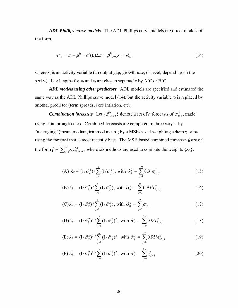
ADL Phillips curve models. The ADL Phillips curve models are direct models of

the form,

ht hπ + − πt = μh + αh(L)Δπt + βh(L)xt + h

t hv + , (14)

where xt is an activity variable (an output gap, growth rate, or level, depending on the

series). Lag lengths for πt and xt are chosen separately by AIC or BIC.

ADL models using other predictors. ADL models are specified and estimated the

same way as the ADL Phillips curve model (14), but the activity variable xt is replaced by

another predictor (term spreads, core inflation, etc.).

Combination forecasts. Let { , |ˆ hi t h tπ + } denote a set of n forecasts of h

t hπ + , made

using data through date t. Combined forecasts are computed in three ways: by

“averaging” (mean, median, trimmed mean); by a MSE-based weighting scheme; or by

using the forecast that is most recently best. The MSE-based combined forecasts ft are of

the form ft = , where six methods are used to compute the weights {λit}: , |1ˆn h

it i t h tiλ π +=∑

(A) λit = 2 2

1

ˆ ˆ(1/ ) / (1/ )n

it jtj

σ σ=∑ , with 2ˆitσ =

392,

0

0.9 ji t j

j

e −=∑ (15)

(B) λit = 2 2

1

ˆ ˆ(1/ ) / (1/ )n

it jtj

σ σ=∑ , with 2ˆitσ =

392,

0

0.95 ji t j

j

e −=∑ (16)

(C) λit = 2 2

1

ˆ ˆ(1/ ) / (1/ )n

it jtj

σ σ=∑ , with 2ˆitσ =

392,

0i t j

j

e −=∑ (17)

(D) λit = σ , with 2ˆit2 2 2 2

1

ˆ ˆ(1/ ) / (1/ )n

it jtj

σ=∑ σ =

392,

0

0.9 ji t j

j

e −=∑ (18)

(E) λit = σ , with 2ˆit2 2 2 2

1

ˆ ˆ(1/ ) / (1/ )n

it jtj

σ=∑ σ =

392,

0

0.95 ji t j

j

e −=∑ (19)

(F) λit = σ , with 2ˆit2 2 2 2

1

ˆ ˆ(1/ ) / (1/ )n

it jtj

σ=∑ σ =

392,

0i t j

j

e −=∑ (20)

26

where ei,t = htπ – is the pseudo out-of-sample forecast error for the ith h-step ahead

forecast and the MSEs are estimated using a 10 year rolling window and, for methods

(A), (B), (D), and (E), discounting.

, |ˆ hi t t hπ −

Inverse MSE weighting (based on population MSEs) is optimal if the individual

forecasts are uncorrelated, and methods (A) – (C) are different ways to implement inverse

MSE weighting. Methods (D) – (F) give greater weight to better-performing forecasts

than does inverse MSE weighting. Optimal forecast combination using regression

weights as in Bates and Granger (1969) is not feasible with the large number of forecasts

under consideration. As Timmerman (2006) notes, equal-weighting (mean combining)

often performs well and Timmerman (2006) provides a discussion of when mean

combining is optimal under squared error loss.

The “recent best” forecasts are the forecasts from the model that has the lowest

cumulative MSE over the past 4 (or, alternatively, 8) quarters.

Finally, in an attempt to exploit the time-varying virtues of the UC-SV and

triangle models, the recent best is computed using just the UC-SV and triangle model

(with time varying NAIRU and z variables).

The complete description of models considered is given in the notes to Table 1.

4.2 Results

The pseudo out-of-sample forecasting performance of each forecasting procedure

(model and combining method) is summarized in tabular and graphical form.

The tabular summary consists of relative RMSEs of four-quarter ahead inflation

forecasts, relative to the UC-SV benchmark, for six forecast periods; these are tabulated

in Tables 1-5 for the five inflation series. The minimum model estimation sample was 40

quarters, and blank cells in the table indicate that for at least one quarter in the forecast

period there were fewer than 40 observations for estimation.

The graphical summary of each model’s performance is given is Figures 6-11 for

the five inflation series. Figure 6 presents the rolling RMSE for the UC-SV benchmark

model for the five inflation series, and figures 7-11 show the RMSE of the various

forecasts relative to the UC-SV benchmark. Part (a) of Figure 7-11 displays the rolling

27

relative RMSE for the prototype models, where the rolling MSE for each model is

computed using (2). Parts (b) – (d) plot the ratio of the rolling RMSE for each category

of models, relative to the UC-SV model: univariate models in part (b), Phillips curve

forecasts (ADL and triangle) in part (c), and combination forecasts in part (d). In each of

parts (b) – (d), leading case models or forecasts are highlighted.

These tables and figures present a great many numbers and facts. Inspection of

these results leads us to the following conclusions:

1. There is strong evidence of time variation in the inflation process, in

predictive relations, and in Phillips curve forecasts. This is consistent with the

literature review, in which different authors reach different conclusions about

Phillips curve forecasts depending on the sample period.

2. The performance of Phillips curve forecasts, relative to the UC-SV

benchmark, has a considerable systematic component (part (c) of the figures):

during periods in which the ADL-u prototype model is forecasting well,

reasonably good forecasts can be made using a host of other activity variables.

In this sense, the choice of activity variable is secondary to the choice of

whether one should use an activity-based forecast.

3. Among the univariate models considered here, with and without time-varying

coefficients, there is no single model, or combination of univariate models,

that has uniformly better performance than the UC-SV model. Of the 82 cells

in Table 1 that give relative RMSEs for univariate CPI-all forecasts in

different subsamples, only 4 have RMSEs less than 1.00, the lowest of which

is .95, and these instances are for fixed-parameter MA models in the 1960s

and in 1985-1992. Similar results are found for the other four inflation

measures. In some cases, the AR models do quite poorly relative to the UC-

SV, for example in the 2001-2007 sample the AR forecasts of CPI-all and

PCE-all inflation have very large relative MSEs (typically exceeding 1.3). In

general, the performance of the AR model, relative to the UC-SV (or AO)

28

benchmarks, is series- and period-specific. This reinforces the remarks in the

literature review about the importance of using a consistently good

benchmark: in some cases, apparently good performance of a predictor for a

particular inflation series over a particular period can be the result of a large

denominator, not a small numerator.

4. Although some of the Phillips curve forecasts improved substantially on the

UC-SV model during the 1970s and early 1980s, there is little or no evidence

that it is possible to improve upon the UC-SV model on average over the full

later samples. This said, there are notable periods and inflation measures for

which Phillips curve models do quite well. The triangle model does

particularly well during the high unemployment disinflation of the early 1980s

for all five inflation measures. For CPI-all, PCE-all, and the GDP deflator, it

also does well in the late 1990s, while for CPI-core and PCE-core the triangle

model does well emerging from the 1990 recession. This episodically good

behavior of the triangle model, and of Phillips-curve forecasts more generally,

provides a more nuanced interpretation of the history of inflation forecasting

models than the blanket Atkeson-Ohanian (2001) conclusion that “none of the

NAIRU forecasts is more accurate than the naïve forecast” (AO abstract).

5. Forecast combining, which has worked so well in other applications

(Timmerman (2006)), generally improves upon the individual Phillips-curve

forecasts, however the combination forecasts generally do not improve upon

the UC-SV benchmark in the post-1993 periods. For example, for PCI-all, the

mean-combined ADL-activity forecasts have a relative RMSE of .86 over

1977-1982 and .96 over 1985-1992; these mean-combined forecasts compare

favorably to individual activity forecasts and to the triangle model. In the

later periods, however, the forecasts being combined have relative RMSEs

exceeding one and combining them works no magic and fails to improve upon

the UC-SV benchmark. Although some of the combining methods improve

upon equal weighting, these improvements are neither large nor systematic.

29

In addition, consistent with the results in Fisher, Liu, and Zhou (2002), factor

forecasts (using the CFNAI) fail to improve upon the UC-SV benchmark on

average over the later periods. These results are consistent with the lack of

success found by attempts in the literature (before and after Atkeson-Ohanian

(2001)) to obtain large gains by using many predictors and/or model

combinations.

6. Forecasts using predictors other than activities variables, while not the main

focus of this paper, generally fare poorly, especially during the post-1992

period. For example, the relative RMSE of the mean-combined forecast using

non-activity variables is at least 0.99 in each subsample in Tables 1-5 for

forecasts of all five activity variables. We did not find substantial

improvements using alternative measures of core (median and trimmed mean

CPI) as predictors.8 Although our treatment of non-activity variables is not

comprehensive, these results largely mirror those in the literature.

5. When Were Phillips Curve Forecasts Successful, and Why?

If the relative performance of Phillips curve forecasts has been episodic, is it

possible to characterize what makes for a successful or unsuccessful episode?

The relative RMSEs of the triangle and ADL-u model forecasts for headline

inflation (CPI-all, PCE-all, and GDP deflator), relative to the UC-SV benchmark, are

plotted in Figure 12, along with the unemployment rate. One immediately evident

feature is that the triangle model has substantially larger swings in performance than the

ADL-u model. This said, the dates of relative success of these Phillips curve forecasts

bear considerable similarities across models and inflation series. Both models perform 8 The exceptions are median and trimmed mean rolling forecasts for CPI-core and GDP inflation for the 2001-2007 sample. However, the relative RMSEs exceed one (typically, they exceed 1.15) for other inflation series, other samples, and for recursive forecasts, and we view these isolated cases as outliers. Most likely, the difference between our negative results for median CPI and Smith’s (2004) positive results over 1990-2000 are differences in the benchmark model, in her case a univariate AR with exponential lag structure imposed.

30

relatively well for all series in the early 1980s, in the early 1990s, and around 1999; both

models perform relatively poorly around 1985 and in the mid-1990s. These dates of

relative success correspond approximately to dates of different phases of business cycles.

Figure 13 is a scatterplot of the quarterly relative RMSE for the triangle (panel

(a)) and ADL-u (panel (b)) prototype models, vs. the two-sided unemployment gap (the

two-sided gap was computed using the two-sided version of the lowpass filter described

in Section 2.3), along with kernel regression estimates. The most striking feature of these

scatterplots is that the relative RMSE is minimized, and is considerably less than one, at

the extremes values of the unemployment gap, both positive and negative. (The kernel

regression estimator exceeds one at the most negative values of the unemployment gap

for the triangle model in panel (a), but there are few observations in that tail.) When the

unemployment rate is near the NAIRU (as measured by the lowpass filter), both Phillips

curve models do worse than the UC-SV model. But when the unemployment gap

exceeds 1.5 in absolute value, the Phillips curve forecasts improve substantially upon the

UC-SV model. Because the gap is largest in absolute value around turning points, this

finding can be restated that the Phillips curve models provide improvements over the UC-

SV model around turning points, but not during normal times.

Figure 14 takes a different perspective on the link between performance of the

Phillips curve forecasts and the state of the economy, by plotting the relative RMSE

against the four-quarter change in the unemployment rate. The relative improvements in

the Phillips curve forecasts do not seem as closely tied to the change in the

unemployment rate as to the gap (the apparent improvement at very high changes of the

unemployment rate is evident in only a few observations)

Figures 15-17 examine a conjecture in the literature, that Phillips curve forecasts

are relatively more successful when inflation is volatile, by plotting the rolling relative

RMSE against the 4-quarter change in 4-quarter inflation. These figures provide only

limited support for this conjecture, as do similar scatterplots (not provided here) of the

rolling RMSE against the UC-SV estimate of the instantaneous variance of the first

difference of the inflation rate. It is true that the quarters of worst performance occur

when in fact inflation is changing very little but, other than for GDP deflator, the

31

episodes of best performance do not seem to be associated with large changes in

inflation.

As presented here, these patterns cannot yet be used to improve forecasts: the

sharpest patterns are ones that appear using two-sided gaps. Still, these results are

suggestive, and they seem to suggest a route toward developing a response to the AO

conundrum in which real economic activity seems to play little or any role in inflation

forecasting. The results here suggest that, if times are quiet – if the unemployment rate is

close to the NAIRU – then in fact one is better off using a univariate forecast than

introducing additional estimation error by making a multivariate forecast. But if the

economy is near a turning point – if the unemployment rate is far from the NAIRU – then

knowledge of that large unemployment gap would be useful for inflation forecasting.

Further work is needed to turn these observations into formal empirical results.

32

References Ang, A., G. Bekaert, and M. Wei (2007), “Do Macro Variables, Asset Markets, or

Surveys Forecast Inflation Better?” Journal of Monetary Economics 54, 1163-1212.

Ascari, Guido and Emanuela Marrocu (2003), “Forecasting Inflation: A Comparison of

Linear Phillips Curve Models and Nonlinear Time Series Models,” Working Paper CRENoS 200307, Centre for North South Economic Research, University of Cagliari and Sassari, Sardinia.

Atkeson, A. and L.E. Ohanian (2001), “Are Phillips Curves Useful for Forecasting

Inflation?” Federal Reserve Bank of Minneapolis Quarterly Review 25(1):2-11. Ball, Laurence M. (2006), “Has Globalization Changed Inflation?” NBER Working

Paper 12687. Bańbura, Marta, Domenico Gianonne, and Lucrezia Reichlin (2008). “Large Bayesian

VARs,” forthcoming, Journal of Applied Econometrics. Banerjee, Anindya and Massimiliano Marcellino (2006), “Are There Any Reliable

Leading Indicators for U.S. Inflation and GDP Growth?,” International Journal of Forecasting 22, 137-151.

Barsky, R.B. (1987), “The Fisher Hypothesis and the Forecastability and Persistence of

Inflation,” Journal of Monetary Economics 19:3-24. Bates, J.M. and Clive W.J. Granger (1969). “The Combination of Forecasts,” Operations

Research Quarterly 20, 451-468. Berardi, Andrea (2007), “Term Structure, Inflation, and Real Activity,” Journal of

Financial and Quantitative Analysis, forthcoming. Bernanke, B.S., J. Bovian and P. Eliasz (2005), “Measuring the effects of monetary

policy: a factor-augmented vector autoregressive (FAVAR) approach”, Quarterly Journal of Economics 120:387-422.

Boivin, Jean and Serena Ng (2005). “Understanding and Comparing Factor-Based

Forecasts,” International Journal of Central Banking 1, 117-151. Boivin, Jean and Serena Ng (2006). “Are More Data Always Better for Factor Analysis?”

Journal of Econometrics 132, 169-194. Bos, Charles S., Philip Hans Franses, and Marius Ooms (2002), “Inflation, Forecast

Intervals and Long Memory Regression Models, International Journal of Forecasting 18, 243-264.

33

Brainard, William and George Perry (2000). “Making Policy in a Changing World.” in

Perry, George and James Tobin (eds), Economic Events, Ideas, and Policies: The 1960s and After. Brookings Institution Press: Washington.

Brave, Scott and Jonas D.M. Fisher (2004), “In Search of a Robust Inflation Forecast,”

Federal Reserve Bank of Chicago Economic Perspectives, 2004Q4, 12-31. Bryan, Michael F. and Stephen G. Cecchetti (1994). “Measuring Core Inflation” in N.

Gregory Mankiw (ed.), Monetary Policy (Chicago: University of Chicago Press for NBER), 195-215.

Bryan, Michael F., Stephen G. Cecchetti, and Rodney L. Wiggins II (1997). “Efficient

Inflation Estimation,” NBER Working Paper No. 6183. Camba-Mendez, Gonazlo and Diego Rodriguez-Palenzuela (2003), “Assessment Criteria

for Output Gap Estimates,” Economic Modeling 20, 529-562 (first published as ECB Working Paper no. 54, 2001).

Canova, Fabio (2007), “G-7 Inflation Forecasts: Random Walk, Phillips Curve, or What

Else?,” Macroeconomic Dynamics 11, 1-30. Cecchetti, Stephen G. (2005), “Inflation Indicators and Inflation Policy,” NBER

Macroeconomics Annual 10, 189-219. Cecchetti, Stephen G., Rita S. Chu, and Charles Steindel (2000), “The Unreliability of

Inflation Indicators,” Federal Reserve Bank of New York Current Issues in Economics and Finance, 6 (4), 1-6.

Cecchetti, Stephen G., Peter Hooper, Bruce C. Kasman, Kermit L. Schoenholtz, and

Mark W. Watson (2007). “Understanding the Evolving Inflation Process,” U.S. Monetary Policy Forum.

Clark, Todd E. and Michael W. McCracken (2006), “'The Predictive Content of the

Output Gap for Inflation: Resolving In-Sample and Out-of-Sample Evidence,” Journal of Money, Credit and Banking 38: 1127-1148.

Clark, Todd E. and Michael W. McCracken (2006), “Combining Forecasts from Nested

Models,” manuscript, Federal Reserve Bank of Kansas City. Cogley, Timothy and Thomas J. Sargent (2002). “Evolving Post-World War II U.S.

Inflation Dynamics,” NBER Macroeconomics Annual 2001, MIT Press, Cambridge.

34

Cogley, Timothy and Thomas J. Sargent (2005). “Drifts and Volatilities: Monetary Policies and Outcomes in the Post World War II U.S.” Review of Economic Dynamics 8, 262-302.

D’Agostino, A. and Domenico Giannone (2006). “Comparing Alternative Predictors

Based on Large-Panel Factor Models,” ECB Working Paper 680. Dielbold, F. and R. Mariano (1995). “Comparing Predictive Accuracy,” Journal of

Business and Economic Statistics 13, 253-265. DeWachter, Hans and Marco Lyrio (2006). “Macro Factors and the Term Structure of

Interest Rates,” Journal of Money, Credit, and Banking 38, 119-140. Diron, Marie and Benoît Mojon (2008). “Are Inflation Targets Good Inflation

Forecasts?” Economic Perspectives, Federal Reserve Bank of Chicago, 2008 Q2, 33-45.

Dupasquier, Chantal, and Nicholas Ricketts (1998). “Nonlinearities in the Output-

Inflation Relationship," in Price Stability, Inflation Targets and Monetary Policy, Ottawa: Bank of Canada.

Eichmeier, Sandra and Christina Ziegler (2006), “How Good are Dynamic Factor Models

at Forecasting Output and Inflation? A Meta-Analytic Approach,” manuscript, Deutsche Bundesbank.

Estrella, Arturo. (2005), “Why Does the Yield Curve Predict Output and Inflation,” The

Economic Journal 115:722-744. Estrella, Arturo and Jeffrey Fuhrer (2003), “Monetary Policy Shifts and the Stability of

Monetary Policy Models,” Review of Economics and Statistics. 85(1): 94-104. Federal Reserve Bank of Chicago (various dates), “The Chicago Fed National Activity

Index,” http://www.chicagofed.org/economic_research_and_data/cfnai.cfm. Fisher, Jonas D.M., C.T. Liu, and R. Zhou (2002), “When Can We Forecast Inflation?”

Federal Reserve Bank of Chicago Economic Perspectives 1Q/2002, 30-42. Gavin, W.T. and K.L. Kliesen (2008). “Forecasting Inflation and Output: Comparing

Data-Rich Models with Simple Rules,” Federal Reserve Bank of St. Louis Review, May/June 2008, 90(3, Part 1), pp. 175-92.

Geweke, John (1977). “The Dynamic Factor Analysis of Economic Time Series,” in: D.J.

Aigner and A.S. Goldberger, eds., Latent Variables in Socio-Economic Models, (North-Holland, Amsterdam).

35

Giacomini, Rafaella, and Halbert White (2006). “Tests of Conditional Predictive Ability,” Econometrica 74, 1545-1578.

Gordon, Robert J. (1982). “Inflation, Flexible Exchange Rates, and the Natural Rate of

Unemployment.” in Workers, Jobs and Inflation, Martin N. Baily (ed). Washington, D.C.: The Brookings Institution,. 89-158.

Gordon, Robert J. and Stephen R. King (1982). “The Output Cost of Disinflation in

Traditional and Vector Autoregressive Models,” Brookings Papers on Economic Activity 1982:I, 205-244.

Gordon, Robert J. (1990). "U.S. Inflation, Labor's Share, and the Natural Rate of Un-

employment." In Economics of Wage Determination (Heinz Konig, ed.). Berlin: Springer-Verlag.

Gordon, Robert J. (1998). Foundations of the Goldilocks Economy: Supply Shocks and

the Time-Varying NAIRU,” Brookings Papers on Economic Activity 1998:2, 297-333.

Hansen, Peter R. (2006), “A Test for Superior Predictive Ability,” Journal of Business

and Economic Statistics 23(4), 365-380. Hardouvelis, Gikas and Dimitrios Malliaropulos, “The Yield Spread as a Symmetric

Predictor of Output and Inflation, manuscript, CEPR Hendry, D.F., and M.P. Clements (2002), “Pooling of forecasts”, Econometrics Journal

5:1-26. Hendry, David F. and Kirstin Hubrich (2007). “Combining Disaggregate Forecasts or

Combining Disaggregate Information to Forecast an Aggregate,” manuscript, Oxford University.

Hubrich, Kirstin (2005). “Forecasting Euro Area Inflation: Does Aggregating Forecasts

by HICP Component Improve Forecast Accuracy?” International Journal of Forecasting 21, 119-136.

Ihrig, Jane, Steve Kamin, and Jaime Marquez (2007), “Some Simple Tests of the

Globalization and Inflation Hypothesis,” Board of Governors of the Federal Reserve System, International Finance Discussion Paper no. 891.

Inoue, Atsushi and Lutz Kilian (2008), “How Useful is Bagging in Forecasting Economic

Time Series? A Case Study of U.S. CPI Inflation,” Journal of the American Statistical Association, forthcoming

Inflation Persistence Network (2007): see

http://www.ecb.eu/home/html/researcher_ipn_papers.en.html

36

Jaditz, Ted and Chera Sayers (1994), “Predicting Inflation,” manuscript, Bureau of Labor

Statistics. Jorion, Philippe and Frederic S. Mishkin. 1991. “A Multi-Country Comparison of Term

Structure Forecasts at Long Horizons,” Journal of Financial Economics 29, pp. 59 – 80.

Koenig, Evan F. (2003), “Is the Markup a Useful Real-Time Predictor of Inflation?,”

Economics Letters 80, 261-267. Lansing, Kevin (2002), “Can the Phillips Curve Help Forecast Inflation?,” Federal

Reserve Bank of San Francisco Economic Letter 2002-29. Laxton, Douglas, David Rose, and Demosthenes Tambakis (1999). “The U.S. Phillips

Curve: The Case for Asymmetry,” Journal of Econ omic Dynamics and Control 23, 1459-1485.

Levin, Andrews and Jeremy Piger (2004). “Is Inflation Persistence Intrinsic in Industrial

Economice?” ECB Working Paper 334. Lown, Cara S. and Robert W. Rich (1997), “Is There an Inflation Puzzle?,” Federal

Reserve Bank of New York Economic Policy Review, December 1997, 51-69. Marcellino, Massimiliano (2008) “A Benchmark Model for Growth and Inflation”,

Journal of Forecasting, forthcoming. Mishkin, Frederic S. (1990a) “What Does the Term Structure Tell Us About Future

Inflation?” Journal of Monetary Economics 25, pp. 77 – 95. Mishkin, Frederic S. (1990b). “The Information in the Longer-Maturity Term Structure

About Future Inflation,” Quarterly Journal of Economics 55, pp. 815 – 828. Mishkin, Frederic S. (1991). “A Multi-Country Study of the Information in the Term

Structure About Future Inflation,” Journal of International Money and Finance 19, pp. 2 – 22.

Mishkin, Frederic S. (2007), “Inflation Dynamics,” NBER Working Paper 13147. Moshiri, Saeed and Norman Cameron (2000). “Neural Network Versus Econometric

Models in Forecasting Inflation,” Journal of Forecasting 19, 201-217. Nason, James M. (2006). “Instability in U.S. Inflation: 1967-2005,” Federal Reserve

Bank of Atlanta Economic Review 2006, 2nd quarter, 39-59

37

Nelson, C.R. and G.W. Schwert (1977), “Short-Term Interest Rates as Predictors of Inflation: On Testing the Hypothesis that the Real Rate of Interest Is Constant,” American Economic Review 67:478-486.

Orphanides, A. and S. van Norden (2005), “The Reliability of Inflation Forecast Based

on Output Gap Estimates in Real Time,” Journal of Money, Credit, and Banking 37:583-600.

Pivetta , Frederic and Ricardo Reis (2007). “The Persistence of Inflation in the United

States,” Journal of Economic Dynamics and Control, 31 (4), 1326-1358. Primiceri, Giorgio (2006). “Why Inflation Rose and Fell: Policymakers’ Beliefs and US

Postwar Stabilization Policy,” The Quarterly Journal of Economics 121, 867-901. Reis, Ricardo and Mark W. Watson (2007). “Relative Goods’ Prices and Pure Inflation,”

manuscript, Princeton University. Roberts, J.M. (2004), “Monetary Policy and Inflation Dynamics,” FEDS Discussion

Paper 2004-62, Federal Reserve Board. Rünstler, Gerhard (2002). “The Information Content of Real-Time Output Gap Estimates:

An Application to the Euro Area,” ECB Working Paper 182. Sargent, Thomas J., and Christopher A. Sims (1977), “Business cycle modeling without

pretending to have too much a-priori economic theory,” in: C. Sims et al., eds., New Methods in Business Cycle Research (Federal Reserve Bank of Minneapolis, Minneapolis).

Sims, Christopher A. and Tao Zha (2004). “Were there Regime Switches in U.S.

Monetary Policy?” manuscript, Princeton University. Smith, Julie K. (2004), “Weighted Median Inflation: Is This Core Inflation?,” Journal of

Money, Credit and Banking 36(2), 253-263. Staiger, Doug, James H. Stock, and Mark W. Watson (1997), “The NAIRU,

Unemployment, and Monetary Policy,” Journal of Economic Perspectives, 11 (Winter 1997), 33-51.

Stock, J.H., and M.W. Watson (1999), “Forecasting Inflation,” Journal of Monetary

Economics 44:293-335. Stock, J.H., and M.W. Watson (2002). “Forecasting Using Principal Components from a

Large Number of Predictors,” Journal of the American Statistical Association 97:1167–1179.

38

Stock, J.H., and M.W. Watson (2003), “Forecasting output and inflation: The role of asset prices,” Journal of Economic Literature 41:788-829.

Stock, J.H., and M.W. Watson (2007), “Why Has U.S. Inflation Become Harder to

Forecast?” Journal of Money, Credit, and Banking 39, 3-34. Stockton, David J. and James E. Glassman (1987). “An Evaluation of the Forecast

Performance of Alternative Models of Inflation,” The Review of Economics and Statistics 69, 108-117.

Taylor, John (2000). “Low Inflation, Pass-Through, and the Pricing Power of Firms,”

European Economic Review 44, 1389-1408. Timmermann, Alan (2006). “Forecast Combinations,” in Handbook of Economic

Forecasting, in Graham Elliott, Clive W.J. Granger and Allan Timmermann (eds.). Elsevier.

Tkacz, Greg (2000), “Non-Parametric and Neural Network Models of Inflation

Changes,” Bank of Canada Working Paper 2000-7 Watson, Mark W. (2003). “Macroeconomic Forecasting Using Many Predictors.” In

Dewatripont, M., L. Hansen, and S. Turnovski (eds), Advances in Econometrics: Theory and Applications, Eighth World Congress of the Econometric Society, Vol. III, 87-115.

Webb, Roy H. and Tazewell S. Rowe (1995), “An Index of Leading Indicators for

Inflation,” Federal Reserve Bank of Richmond Economic Quarterly 81(2), 75-96. West, K. (1996). “Asymptotic Inference about Predictive Accuracy,” Econometrica 64,

1067-1084. Wright, Jonathan (2003), “Forecasting U.S. Inflation by Bayesian Model Averaging,”

Board of Governors of the Federal Reserve System International Finance Discussion Paper no. 780.

39

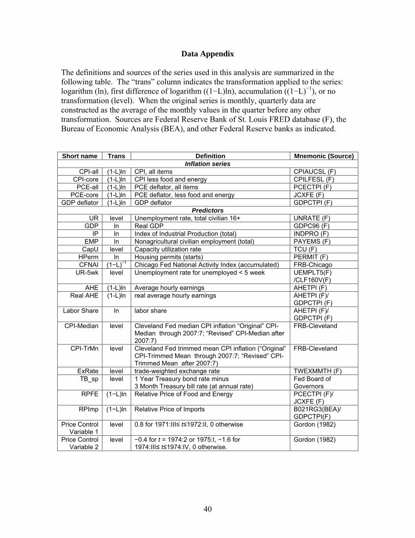
Data Appendix The definitions and sources of the series used in this analysis are summarized in the following table. The “trans” column indicates the transformation applied to the series: logarithm (ln), first difference of logarithm ((1−L)ln), accumulation ((1−L)−1), or no transformation (level). When the original series is monthly, quarterly data are constructed as the average of the monthly values in the quarter before any other transformation. Sources are Federal Reserve Bank of St. Louis FRED database (F), the Bureau of Economic Analysis (BEA), and other Federal Reserve banks as indicated. Short name Trans Definition Mnemonic (Source)

Inflation series CPI-all (1-L)ln CPI, all items CPIAUCSL (F)

CPI-core (1-L)ln CPI less food and energy CPILFESL (F) PCE-all (1-L)ln PCE deflator, all items PCECTPI (F)

PCE-core (1-L)ln PCE deflator, less food and energy JCXFE (F) GDP deflator (1-L)ln GDP deflator GDPCTPI (F)

Predictors UR level Unemployment rate, total civilian 16+ UNRATE (F)

GDP ln Real GDP GDPC96 (F) IP ln Index of Industrial Production (total) INDPRO (F)

EMP ln Nonagricultural civilian employment (total) PAYEMS (F) CapU level Capacity utilization rate TCU (F)

HPerm ln Housing permits (starts) PERMIT (F) CFNAI (1−L)−1 Chicago Fed National Activity Index (accumulated) FRB-Chicago

UR-5wk level Unemployment rate for unemployed < 5 week UEMPLT5(F) /CLF160V(F)

AHE (1-L)ln Average hourly earnings AHETPI (F) Real AHE (1-L)ln real average hourly earnings AHETPI (F)/

GDPCTPI (F) Labor Share ln labor share AHETPI (F)/

GDPCTPI (F) CPI-Median level Cleveland Fed median CPI inflation “Original” CPI-

Median through 2007:7; “Revised” CPI-Median after 2007:7)

FRB-Cleveland

CPI-TrMn level Cleveland Fed trimmed mean CPI inflation (“Original” CPI-Trimmed Mean through 2007:7; “Revised” CPI-Trimmed Mean after 2007:7)

FRB-Cleveland

ExRate level trade-weighted exchange rate TWEXMMTH (F) TB_sp level 1 Year Treasury bond rate minus

3 Month Treasury bill rate (at annual rate) Fed Board of Governors

RPFE (1−L)ln Relative Price of Food and Energy PCECTPI (F)/ JCXFE (F)

RPImp (1−L)ln Relative Price of Imports B021RG3(BEA)/ GDPCTPI(F)

Price Control Variable 1

level 0.8 for 1971:III≤ t≤1972:II, 0 otherwise Gordon (1982)

Price Control Variable 2

level −0.4 for t = 1974:2 or 1975:I, −1.6 for 1974:III≤ t≤1974:IV, 0 otherwise.

Gordon (1982)

40

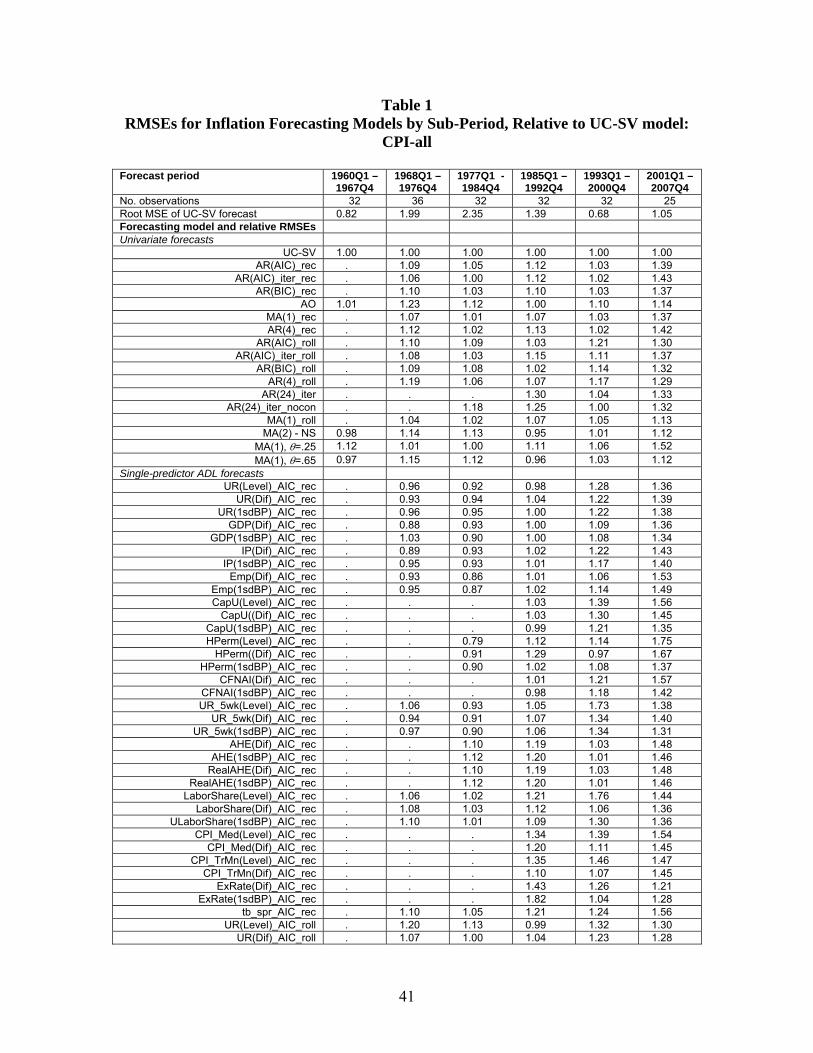
Table 1 RMSEs for Inflation Forecasting Models by Sub-Period, Relative to UC-SV model:

CPI-all Forecast period 1960Q1 –

1967Q4 1968Q1 – 1976Q4

1977Q1 - 1984Q4

1985Q1 – 1992Q4

1993Q1 – 2000Q4

2001Q1 – 2007Q4

No. observations 32 36 32 32 32 25 Root MSE of UC-SV forecast 0.82 1.99 2.35 1.39 0.68 1.05 Forecasting model and relative RMSEs Univariate forecasts

UC-SV 1.00 1.00 1.00 1.00 1.00 1.00 AR(AIC)_rec . 1.09 1.05 1.12 1.03 1.39

AR(AIC)_iter_rec . 1.06 1.00 1.12 1.02 1.43 AR(BIC)_rec . 1.10 1.03 1.10 1.03 1.37

AO 1.01 1.23 1.12 1.00 1.10 1.14 MA(1)_rec . 1.07 1.01 1.07 1.03 1.37 AR(4)_rec . 1.12 1.02 1.13 1.02 1.42

AR(AIC)_roll . 1.10 1.09 1.03 1.21 1.30 AR(AIC)_iter_roll . 1.08 1.03 1.15 1.11 1.37

AR(BIC)_roll . 1.09 1.08 1.02 1.14 1.32 AR(4)_roll . 1.19 1.06 1.07 1.17 1.29

AR(24)_iter . . . 1.30 1.04 1.33 AR(24)_iter_nocon . . 1.18 1.25 1.00 1.32

MA(1)_roll . 1.04 1.02 1.07 1.05 1.13 MA(2) - NS 0.98 1.14 1.13 0.95 1.01 1.12

MA(1), θ=.25 1.12 1.01 1.00 1.11 1.06 1.52 MA(1), θ=.65 0.97 1.15 1.12 0.96 1.03 1.12

Single-predictor ADL forecasts UR(Level)_AIC_rec . 0.96 0.92 0.98 1.28 1.36

UR(Dif)_AIC_rec . 0.93 0.94 1.04 1.22 1.39 UR(1sdBP)_AIC_rec . 0.96 0.95 1.00 1.22 1.38

GDP(Dif)_AIC_rec . 0.88 0.93 1.00 1.09 1.36 GDP(1sdBP)_AIC_rec . 1.03 0.90 1.00 1.08 1.34

IP(Dif)_AIC_rec . 0.89 0.93 1.02 1.22 1.43 IP(1sdBP)_AIC_rec . 0.95 0.93 1.01 1.17 1.40

Emp(Dif)_AIC_rec . 0.93 0.86 1.01 1.06 1.53 Emp(1sdBP)_AIC_rec . 0.95 0.87 1.02 1.14 1.49 CapU(Level)_AIC_rec . . . 1.03 1.39 1.56

CapU((Dif)_AIC_rec . . . 1.03 1.30 1.45 CapU(1sdBP)_AIC_rec . . . 0.99 1.21 1.35 HPerm(Level)_AIC_rec . . 0.79 1.12 1.14 1.75

HPerm((Dif)_AIC_rec . . 0.91 1.29 0.97 1.67 HPerm(1sdBP)_AIC_rec . . 0.90 1.02 1.08 1.37

CFNAI(Dif)_AIC_rec . . . 1.01 1.21 1.57 CFNAI(1sdBP)_AIC_rec . . . 0.98 1.18 1.42 UR_5wk(Level)_AIC_rec . 1.06 0.93 1.05 1.73 1.38

UR_5wk(Dif)_AIC_rec . 0.94 0.91 1.07 1.34 1.40 UR_5wk(1sdBP)_AIC_rec . 0.97 0.90 1.06 1.34 1.31

AHE(Dif)_AIC_rec . . 1.10 1.19 1.03 1.48 AHE(1sdBP)_AIC_rec . . 1.12 1.20 1.01 1.46

RealAHE(Dif)_AIC_rec . . 1.10 1.19 1.03 1.48 RealAHE(1sdBP)_AIC_rec . . 1.12 1.20 1.01 1.46

LaborShare(Level)_AIC_rec . 1.06 1.02 1.21 1.76 1.44 LaborShare(Dif)_AIC_rec . 1.08 1.03 1.12 1.06 1.36

ULaborShare(1sdBP)_AIC_rec . 1.10 1.01 1.09 1.30 1.36 CPI_Med(Level)_AIC_rec . . . 1.34 1.39 1.54

CPI_Med(Dif)_AIC_rec . . . 1.20 1.11 1.45 CPI_TrMn(Level)_AIC_rec . . . 1.35 1.46 1.47

CPI_TrMn(Dif)_AIC_rec . . . 1.10 1.07 1.45 ExRate(Dif)_AIC_rec . . . 1.43 1.26 1.21

ExRate(1sdBP)_AIC_rec . . . 1.82 1.04 1.28 tb_spr_AIC_rec . 1.10 1.05 1.21 1.24 1.56

UR(Level)_AIC_roll . 1.20 1.13 0.99 1.32 1.30 UR(Dif)_AIC_roll . 1.07 1.00 1.04 1.23 1.28

41

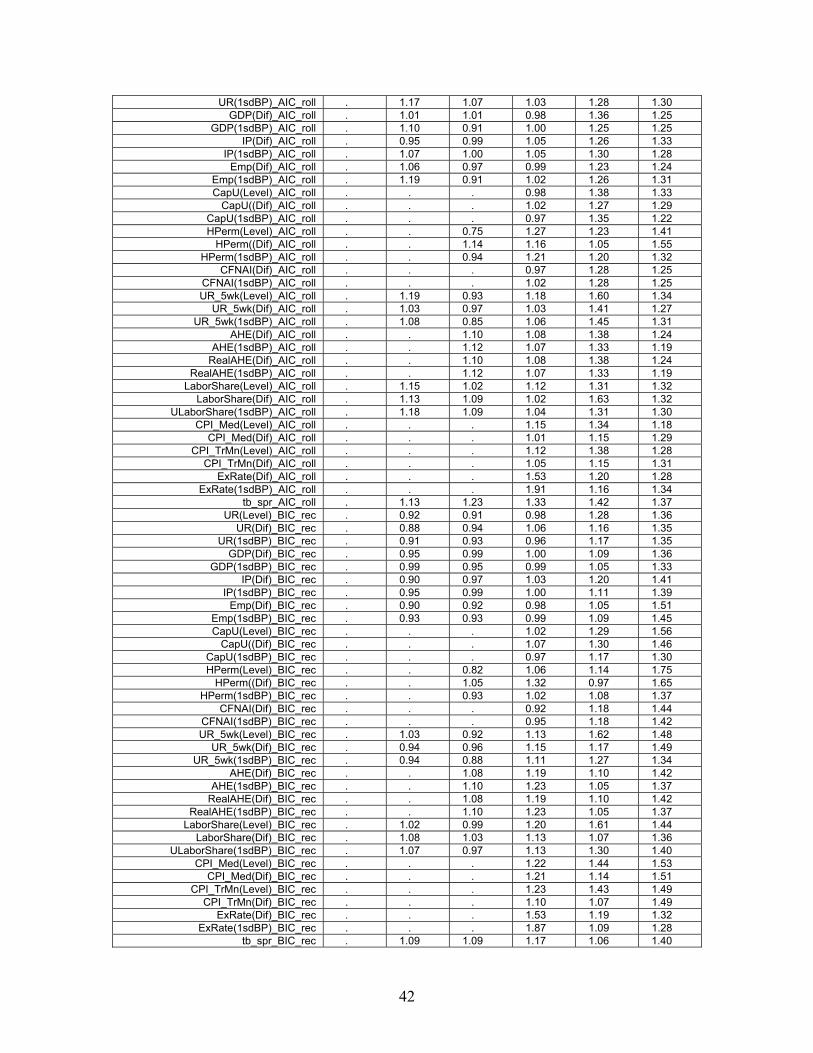
UR(1sdBP)_AIC_roll . 1.17 1.07 1.03 1.28 1.30 GDP(Dif)_AIC_roll . 1.01 1.01 0.98 1.36 1.25

GDP(1sdBP)_AIC_roll . 1.10 0.91 1.00 1.25 1.25 IP(Dif)_AIC_roll . 0.95 0.99 1.05 1.26 1.33

IP(1sdBP)_AIC_roll . 1.07 1.00 1.05 1.30 1.28 Emp(Dif)_AIC_roll . 1.06 0.97 0.99 1.23 1.24

Emp(1sdBP)_AIC_roll . 1.19 0.91 1.02 1.26 1.31 CapU(Level)_AIC_roll . . . 0.98 1.38 1.33

CapU((Dif)_AIC_roll . . . 1.02 1.27 1.29 CapU(1sdBP)_AIC_roll . . . 0.97 1.35 1.22 HPerm(Level)_AIC_roll . . 0.75 1.27 1.23 1.41

HPerm((Dif)_AIC_roll . . 1.14 1.16 1.05 1.55 HPerm(1sdBP)_AIC_roll . . 0.94 1.21 1.20 1.32

CFNAI(Dif)_AIC_roll . . . 0.97 1.28 1.25 CFNAI(1sdBP)_AIC_roll . . . 1.02 1.28 1.25 UR_5wk(Level)_AIC_roll . 1.19 0.93 1.18 1.60 1.34

UR_5wk(Dif)_AIC_roll . 1.03 0.97 1.03 1.41 1.27 UR_5wk(1sdBP)_AIC_roll . 1.08 0.85 1.06 1.45 1.31

AHE(Dif)_AIC_roll . . 1.10 1.08 1.38 1.24 AHE(1sdBP)_AIC_roll . . 1.12 1.07 1.33 1.19

RealAHE(Dif)_AIC_roll . . 1.10 1.08 1.38 1.24 RealAHE(1sdBP)_AIC_roll . . 1.12 1.07 1.33 1.19

LaborShare(Level)_AIC_roll . 1.15 1.02 1.12 1.31 1.32 LaborShare(Dif)_AIC_roll . 1.13 1.09 1.02 1.63 1.32

ULaborShare(1sdBP)_AIC_roll . 1.18 1.09 1.04 1.31 1.30 CPI_Med(Level)_AIC_roll . . . 1.15 1.34 1.18

CPI_Med(Dif)_AIC_roll . . . 1.01 1.15 1.29 CPI_TrMn(Level)_AIC_roll . . . 1.12 1.38 1.28

CPI_TrMn(Dif)_AIC_roll . . . 1.05 1.15 1.31 ExRate(Dif)_AIC_roll . . . 1.53 1.20 1.28

ExRate(1sdBP)_AIC_roll . . . 1.91 1.16 1.34 tb_spr_AIC_roll . 1.13 1.23 1.33 1.42 1.37

UR(Level)_BIC_rec . 0.92 0.91 0.98 1.28 1.36 UR(Dif)_BIC_rec . 0.88 0.94 1.06 1.16 1.35

UR(1sdBP)_BIC_rec . 0.91 0.93 0.96 1.17 1.35 GDP(Dif)_BIC_rec . 0.95 0.99 1.00 1.09 1.36

GDP(1sdBP)_BIC_rec . 0.99 0.95 0.99 1.05 1.33 IP(Dif)_BIC_rec . 0.90 0.97 1.03 1.20 1.41

IP(1sdBP)_BIC_rec . 0.95 0.99 1.00 1.11 1.39 Emp(Dif)_BIC_rec . 0.90 0.92 0.98 1.05 1.51

Emp(1sdBP)_BIC_rec . 0.93 0.93 0.99 1.09 1.45 CapU(Level)_BIC_rec . . . 1.02 1.29 1.56

CapU((Dif)_BIC_rec . . . 1.07 1.30 1.46 CapU(1sdBP)_BIC_rec . . . 0.97 1.17 1.30 HPerm(Level)_BIC_rec . . 0.82 1.06 1.14 1.75

HPerm((Dif)_BIC_rec . . 1.05 1.32 0.97 1.65 HPerm(1sdBP)_BIC_rec . . 0.93 1.02 1.08 1.37

CFNAI(Dif)_BIC_rec . . . 0.92 1.18 1.44 CFNAI(1sdBP)_BIC_rec . . . 0.95 1.18 1.42 UR_5wk(Level)_BIC_rec . 1.03 0.92 1.13 1.62 1.48

UR_5wk(Dif)_BIC_rec . 0.94 0.96 1.15 1.17 1.49 UR_5wk(1sdBP)_BIC_rec . 0.94 0.88 1.11 1.27 1.34

AHE(Dif)_BIC_rec . . 1.08 1.19 1.10 1.42 AHE(1sdBP)_BIC_rec . . 1.10 1.23 1.05 1.37

RealAHE(Dif)_BIC_rec . . 1.08 1.19 1.10 1.42 RealAHE(1sdBP)_BIC_rec . . 1.10 1.23 1.05 1.37

LaborShare(Level)_BIC_rec . 1.02 0.99 1.20 1.61 1.44 LaborShare(Dif)_BIC_rec . 1.08 1.03 1.13 1.07 1.36

ULaborShare(1sdBP)_BIC_rec . 1.07 0.97 1.13 1.30 1.40 CPI_Med(Level)_BIC_rec . . . 1.22 1.44 1.53

CPI_Med(Dif)_BIC_rec . . . 1.21 1.14 1.51 CPI_TrMn(Level)_BIC_rec . . . 1.23 1.43 1.49

CPI_TrMn(Dif)_BIC_rec . . . 1.10 1.07 1.49 ExRate(Dif)_BIC_rec . . . 1.53 1.19 1.32

ExRate(1sdBP)_BIC_rec . . . 1.87 1.09 1.28 tb_spr_BIC_rec . 1.09 1.09 1.17 1.06 1.40

42

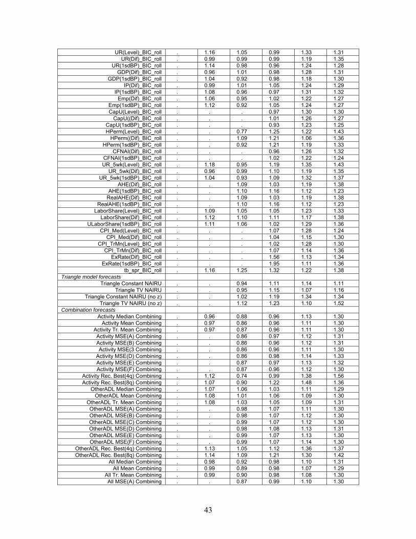
UR(Level)_BIC_roll . 1.16 1.05 0.99 1.33 1.31 UR(Dif)_BIC_roll . 0.99 0.99 0.99 1.19 1.35

UR(1sdBP)_BIC_roll . 1.14 0.98 0.96 1.24 1.28 GDP(Dif)_BIC_roll . 0.96 1.01 0.98 1.28 1.31

GDP(1sdBP)_BIC_roll . 1.04 0.92 0.98 1.18 1.30 IP(Dif)_BIC_roll . 0.99 1.01 1.05 1.24 1.29

IP(1sdBP)_BIC_roll . 1.08 0.96 0.97 1.31 1.32 Emp(Dif)_BIC_roll . 1.06 0.95 1.02 1.22 1.27

Emp(1sdBP)_BIC_roll . 1.12 0.92 1.05 1.24 1.27 CapU(Level)_BIC_roll . . . 0.97 1.30 1.30

CapU((Dif)_BIC_roll . . . 1.01 1.26 1.27 CapU(1sdBP)_BIC_roll . . . 0.93 1.23 1.25 HPerm(Level)_BIC_roll . . 0.77 1.25 1.22 1.43

HPerm((Dif)_BIC_roll . . 1.09 1.21 1.06 1.36 HPerm(1sdBP)_BIC_roll . . 0.92 1.21 1.19 1.33

CFNAI(Dif)_BIC_roll . . . 0.96 1.26 1.32 CFNAI(1sdBP)_BIC_roll . . . 1.02 1.22 1.24 UR_5wk(Level)_BIC_roll . 1.18 0.95 1.19 1.35 1.43

UR_5wk(Dif)_BIC_roll . 0.96 0.99 1.10 1.19 1.35 UR_5wk(1sdBP)_BIC_roll . 1.04 0.93 1.09 1.32 1.37

AHE(Dif)_BIC_roll . . 1.09 1.03 1.19 1.38 AHE(1sdBP)_BIC_roll . . 1.10 1.16 1.12 1.23

RealAHE(Dif)_BIC_roll . . 1.09 1.03 1.19 1.38 RealAHE(1sdBP)_BIC_roll . . 1.10 1.16 1.12 1.23

LaborShare(Level)_BIC_roll . 1.09 1.05 1.05 1.23 1.33 LaborShare(Dif)_BIC_roll . 1.12 1.10 1.11 1.17 1.38

ULaborShare(1sdBP)_BIC_roll . 1.11 1.06 1.02 1.29 1.36 CPI_Med(Level)_BIC_roll . . . 1.07 1.28 1.24

CPI_Med(Dif)_BIC_roll . . . 1.04 1.15 1.30 CPI_TrMn(Level)_BIC_roll . . . 1.02 1.28 1.30

CPI_TrMn(Dif)_BIC_roll . . . 1.07 1.14 1.36 ExRate(Dif)_BIC_roll . . . 1.56 1.13 1.34

ExRate(1sdBP)_BIC_roll . . . 1.95 1.11 1.36 tb_spr_BIC_roll . 1.16 1.25 1.32 1.22 1.38

Triangle model forecasts Triangle Constant NAIRU . . 0.94 1.11 1.14 1.11

Triangle TV NAIRU . . 0.95 1.15 1.07 1.16 Triangle Constant NAIRU (no z) . . 1.02 1.19 1.34 1.34

Triangle TV NAIRU (no z) . . 1.12 1.23 1.10 1.52 Combination forecasts

Activity Median Combining . 0.96 0.88 0.96 1.13 1.30 Activity Mean Combining . 0.97 0.86 0.96 1.11 1.30

Activity Tr. Mean Combining . 0.97 0.87 0.96 1.11 1.30 Activity MSE(A) Combining . . 0.86 0.97 1.12 1.31 Activity MSE(B) Combining . . 0.86 0.96 1.12 1.31 Activity MSE(3 Combining . . 0.86 0.96 1.11 1.30

Activity MSE(D) Combining . . 0.86 0.98 1.14 1.33 Activity MSE(E) Combining . . 0.87 0.97 1.13 1.32 Activity MSE(F) Combining . . 0.87 0.96 1.12 1.30

Activity Rec. Best(4q) Combining . 1.12 0.74 0.99 1.38 1.56 Activity Rec. Best(8q) Combining . 1.07 0.90 1.22 1.48 1.36

OtherADL Median Combining . 1.07 1.06 1.03 1.11 1.29 OtherADL Mean Combining . 1.08 1.01 1.06 1.09 1.30

OtherADL Tr. Mean Combining . 1.08 1.03 1.05 1.09 1.31 OtherADL MSE(A) Combining . . 0.98 1.07 1.11 1.30 OtherADL MSE(B) Combining . . 0.98 1.07 1.12 1.30 OtherADL MSE(C) Combining . . 0.99 1.07 1.12 1.30 OtherADL MSE(D) Combining . . 0.98 1.08 1.13 1.31 OtherADL MSE(E) Combining . . 0.99 1.07 1.13 1.30 OtherADL MSE(F) Combining . . 0.99 1.07 1.14 1.30

OtherADL Rec. Best(4q) Combining . 1.13 1.05 1.12 1.36 1.37 OtherADL Rec. Best(8q) Combining . 1.14 1.09 1.21 1.30 1.42

All Median Combining . 0.98 0.92 0.98 1.10 1.31 All Mean Combining . 0.99 0.89 0.98 1.07 1.29

All Tr. Mean Combining . 0.99 0.90 0.98 1.08 1.30 All MSE(A) Combining . . 0.87 0.99 1.10 1.30

43

All MSE(B) Combining . . 0.87 0.98 1.10 1.30 All MSE(C) Combining . . 0.87 0.98 1.09 1.29 All MSE(D) Combining . . 0.87 1.00 1.12 1.31 All MSE(E) Combining . . 0.88 0.99 1.12 1.30 All MSE(F) Combining . . 0.88 0.98 1.10 1.29

All Rec. Best(4q) Combining . 1.12 0.74 1.11 1.47 1.63 All Rec. Best(8q) Combining . 1.08 0.92 1.19 1.51 1.43

UCSV and Triangle Rec. Best(4q) Combining

. . . 1.02 1.05 1.01

UCSV and Triangle Rec. Best(8q) Combining

. . . 1.06 1.05 1.11

Notes to Table 1: Entries are RMSEs, relative to the RMSE of the UC-SV model, over the indicated sample period. Blanks indicate insufficient data to compute forecasts over the indicated subsample. The abbreviations denote:

_AIC: AIC lag selection, up to six lags (for ADL models, AIC over the two lag lengths separately)

_BIC: BIC lag selection, up to six lags (for ADL models, AIC over the two lag lengths separately)

_rec: recursive estimation _roll: rolling estimation Level: indicated predictor appears in levels Dif: indicated predictor appears in log differences 1sdBP: indicated predictor appears in gap form, computed using 1-sided

bandpass filter as discussed in the text Triangle: Triangle model or TV-triangle model, with or without supply shock

(“z”) variables mean, median, trimmed mean: forecast combining methods, for the indicated

group of forecasts MSE(A) – MSE(F): MSE-based combining as indicated in (15) - (20). Best (4q) and Best (8q): recently best forecast based on cumulative MSE over

past 4 (or 8) quarters UCSV and Triangle Rec. Best (4q) and (8q) Combining: best of UC-SV and

triangle models (constant NAIRU) based on cumulative MSE over past 4 (or 8) quarters

nocon: constant term is suppressed

44

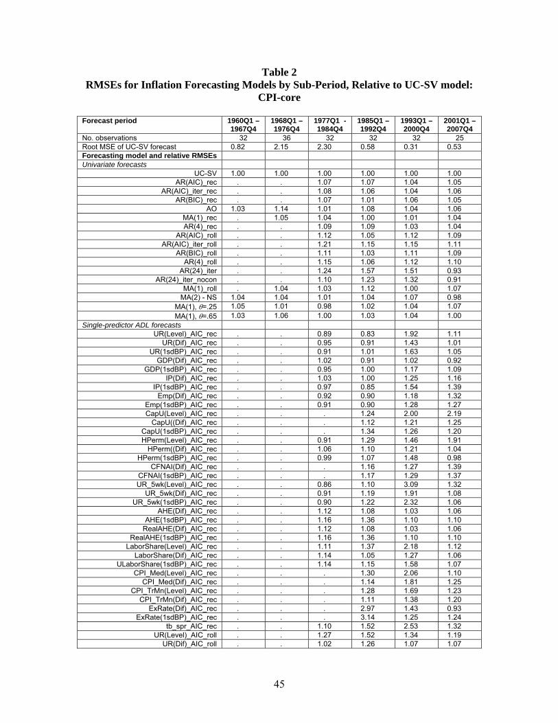
Table 2 RMSEs for Inflation Forecasting Models by Sub-Period, Relative to UC-SV model:

CPI-core Forecast period 1960Q1 –

1967Q4 1968Q1 – 1976Q4

1977Q1 - 1984Q4

1985Q1 – 1992Q4

1993Q1 – 2000Q4

2001Q1 – 2007Q4

No. observations 32 36 32 32 32 25 Root MSE of UC-SV forecast 0.82 2.15 2.30 0.58 0.31 0.53 Forecasting model and relative RMSEs Univariate forecasts

UC-SV 1.00 1.00 1.00 1.00 1.00 1.00 AR(AIC)_rec . . 1.07 1.07 1.04 1.05

AR(AIC)_iter_rec . . 1.08 1.06 1.04 1.06 AR(BIC)_rec . . 1.07 1.01 1.06 1.05

AO 1.03 1.14 1.01 1.08 1.04 1.06 MA(1)_rec . 1.05 1.04 1.00 1.01 1.04 AR(4)_rec . . 1.09 1.09 1.03 1.04

AR(AIC)_roll . . 1.12 1.05 1.12 1.09 AR(AIC)_iter_roll . . 1.21 1.15 1.15 1.11

AR(BIC)_roll . . 1.11 1.03 1.11 1.09 AR(4)_roll . . 1.15 1.06 1.12 1.10

AR(24)_iter . . 1.24 1.57 1.51 0.93 AR(24)_iter_nocon . . 1.10 1.23 1.32 0.91

MA(1)_roll . 1.04 1.03 1.12 1.00 1.07 MA(2) - NS 1.04 1.04 1.01 1.04 1.07 0.98

MA(1), θ=.25 1.05 1.01 0.98 1.02 1.04 1.07 MA(1), θ=.65 1.03 1.06 1.00 1.03 1.04 1.00

Single-predictor ADL forecasts UR(Level)_AIC_rec . . 0.89 0.83 1.92 1.11

UR(Dif)_AIC_rec . . 0.95 0.91 1.43 1.01 UR(1sdBP)_AIC_rec . . 0.91 1.01 1.63 1.05

GDP(Dif)_AIC_rec . . 1.02 0.91 1.02 0.92 GDP(1sdBP)_AIC_rec . . 0.95 1.00 1.17 1.09

IP(Dif)_AIC_rec . . 1.03 1.00 1.25 1.16 IP(1sdBP)_AIC_rec . . 0.97 0.85 1.54 1.39

Emp(Dif)_AIC_rec . . 0.92 0.90 1.18 1.32 Emp(1sdBP)_AIC_rec . . 0.91 0.90 1.28 1.27 CapU(Level)_AIC_rec . . . 1.24 2.00 2.19

CapU((Dif)_AIC_rec . . . 1.12 1.21 1.25 CapU(1sdBP)_AIC_rec . . . 1.34 1.26 1.20 HPerm(Level)_AIC_rec . . 0.91 1.29 1.46 1.91

HPerm((Dif)_AIC_rec . . 1.06 1.10 1.21 1.04 HPerm(1sdBP)_AIC_rec . . 0.99 1.07 1.48 0.98

CFNAI(Dif)_AIC_rec . . . 1.16 1.27 1.39 CFNAI(1sdBP)_AIC_rec . . . 1.17 1.29 1.37 UR_5wk(Level)_AIC_rec . . 0.86 1.10 3.09 1.32

UR_5wk(Dif)_AIC_rec . . 0.91 1.19 1.91 1.08 UR_5wk(1sdBP)_AIC_rec . . 0.90 1.22 2.32 1.06

AHE(Dif)_AIC_rec . . 1.12 1.08 1.03 1.06 AHE(1sdBP)_AIC_rec . . 1.16 1.36 1.10 1.10

RealAHE(Dif)_AIC_rec . . 1.12 1.08 1.03 1.06 RealAHE(1sdBP)_AIC_rec . . 1.16 1.36 1.10 1.10

LaborShare(Level)_AIC_rec . . 1.11 1.37 2.18 1.12 LaborShare(Dif)_AIC_rec . . 1.14 1.05 1.27 1.06

ULaborShare(1sdBP)_AIC_rec . . 1.14 1.15 1.58 1.07 CPI_Med(Level)_AIC_rec . . . 1.30 2.06 1.10

CPI_Med(Dif)_AIC_rec . . . 1.14 1.81 1.25 CPI_TrMn(Level)_AIC_rec . . . 1.28 1.69 1.23

CPI_TrMn(Dif)_AIC_rec . . . 1.11 1.38 1.20 ExRate(Dif)_AIC_rec . . . 2.97 1.43 0.93

ExRate(1sdBP)_AIC_rec . . . 3.14 1.25 1.24 tb_spr_AIC_rec . . 1.10 1.52 2.53 1.32

UR(Level)_AIC_roll . . 1.27 1.52 1.34 1.19 UR(Dif)_AIC_roll . . 1.02 1.26 1.07 1.07

45

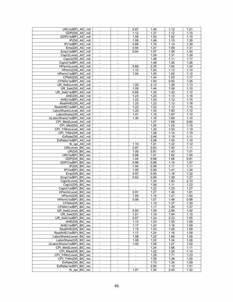
UR(1sdBP)_AIC_roll . . 0.87 1.40 1.12 1.21 GDP(Dif)_AIC_roll . . 1.12 1.37 1.12 1.10

GDP(1sdBP)_AIC_roll . . 1.00 1.52 1.02 1.10 IP(Dif)_AIC_roll . . 1.08 1.48 1.15 1.26

IP(1sdBP)_AIC_roll . . 0.89 1.70 1.14 1.39 Emp(Dif)_AIC_roll . . 0.94 1.47 1.09 1.31

Emp(1sdBP)_AIC_roll . . 0.84 1.57 1.08 1.54 CapU(Level)_AIC_roll . . . 1.59 1.31 1.39

CapU((Dif)_AIC_roll . . . 1.48 1.11 1.17 CapU(1sdBP)_AIC_roll . . . 1.48 1.26 1.26 HPerm(Level)_AIC_roll . . 0.89 2.35 1.04 1.24

HPerm((Dif)_AIC_roll . . 1.10 1.63 1.12 1.14 HPerm(1sdBP)_AIC_roll . . 1.04 1.95 1.05 1.12

CFNAI(Dif)_AIC_roll . . . 1.44 1.03 1.17 CFNAI(1sdBP)_AIC_roll . . . 1.50 0.92 1.25 UR_5wk(Level)_AIC_roll . . 1.05 2.12 1.28 1.13

UR_5wk(Dif)_AIC_roll . . 1.09 1.44 1.08 1.10 UR_5wk(1sdBP)_AIC_roll . . 0.85 1.32 1.33 1.12

AHE(Dif)_AIC_roll . . 1.23 1.23 1.13 1.16 AHE(1sdBP)_AIC_roll . . 1.22 1.53 1.12 1.15

RealAHE(Dif)_AIC_roll . . 1.23 1.23 1.13 1.16 RealAHE(1sdBP)_AIC_roll . . 1.22 1.53 1.12 1.15

LaborShare(Level)_AIC_roll . . 1.20 1.34 1.83 1.12 LaborShare(Dif)_AIC_roll . . 1.41 1.15 1.97 1.10

ULaborShare(1sdBP)_AIC_roll . . 1.30 1.16 1.69 1.10 CPI_Med(Level)_AIC_roll . . . 1.37 1.69 0.80

CPI_Med(Dif)_AIC_roll . . . 1.04 1.25 1.15 CPI_TrMn(Level)_AIC_roll . . . 1.30 1.53 1.19

CPI_TrMn(Dif)_AIC_roll . . . 1.08 1.14 1.19 ExRate(Dif)_AIC_roll . . . 3.48 1.19 1.11

ExRate(1sdBP)_AIC_roll . . . 3.58 1.05 1.10 tb_spr_AIC_roll . . 1.15 1.61 1.22 1.12

UR(Level)_BIC_rec . . 0.97 0.83 1.92 1.11 UR(Dif)_BIC_rec . . 1.00 0.91 1.43 1.01

UR(1sdBP)_BIC_rec . . 0.88 1.01 1.62 1.05 GDP(Dif)_BIC_rec . . 1.04 0.98 1.06 0.91

GDP(1sdBP)_BIC_rec . . 0.96 0.96 1.14 1.07 IP(Dif)_BIC_rec . . 1.04 0.99 1.11 1.11

IP(1sdBP)_BIC_rec . . 1.00 0.90 1.41 1.34 Emp(Dif)_BIC_rec . . 0.97 0.90 1.18 1.32

Emp(1sdBP)_BIC_rec . . 0.83 0.90 1.28 1.27 CapU(Level)_BIC_rec . . . 1.24 1.83 2.10

CapU((Dif)_BIC_rec . . . 1.06 1.11 1.22 CapU(1sdBP)_BIC_rec . . . 1.22 1.23 1.27 HPerm(Level)_BIC_rec . . 0.91 1.27 1.46 1.91

HPerm((Dif)_BIC_rec . . 1.05 1.16 1.21 1.04 HPerm(1sdBP)_BIC_rec . . 0.99 1.07 1.48 0.98

CFNAI(Dif)_BIC_rec . . . 1.10 1.27 1.29 CFNAI(1sdBP)_BIC_rec . . . 1.17 1.29 1.37 UR_5wk(Level)_BIC_rec . . 0.93 1.09 2.88 1.42

UR_5wk(Dif)_BIC_rec . . 1.01 1.19 1.94 1.15 UR_5wk(1sdBP)_BIC_rec . . 0.87 1.24 2.23 1.05

AHE(Dif)_BIC_rec . . 1.13 1.03 1.05 1.09 AHE(1sdBP)_BIC_rec . . 1.17 1.24 1.16 1.09

RealAHE(Dif)_BIC_rec . . 1.13 1.03 1.05 1.09 RealAHE(1sdBP)_BIC_rec . . 1.17 1.24 1.16 1.09

LaborShare(Level)_BIC_rec . . 1.08 1.22 1.68 1.09 LaborShare(Dif)_BIC_rec . . 1.09 1.02 1.34 1.08

ULaborShare(1sdBP)_BIC_rec . . 1.09 1.08 1.27 1.02 CPI_Med(Level)_BIC_rec . . . 1.34 1.66 1.11

CPI_Med(Dif)_BIC_rec . . . 1.02 1.25 1.10 CPI_TrMn(Level)_BIC_rec . . . 1.28 1.71 1.23

CPI_TrMn(Dif)_BIC_rec . . . 1.09 1.38 1.20 ExRate(Dif)_BIC_rec . . . 1.73 1.34 1.09

ExRate(1sdBP)_BIC_rec . . . 2.85 1.10 1.01 tb_spr_BIC_rec . . 1.07 1.50 2.40 1.32

46

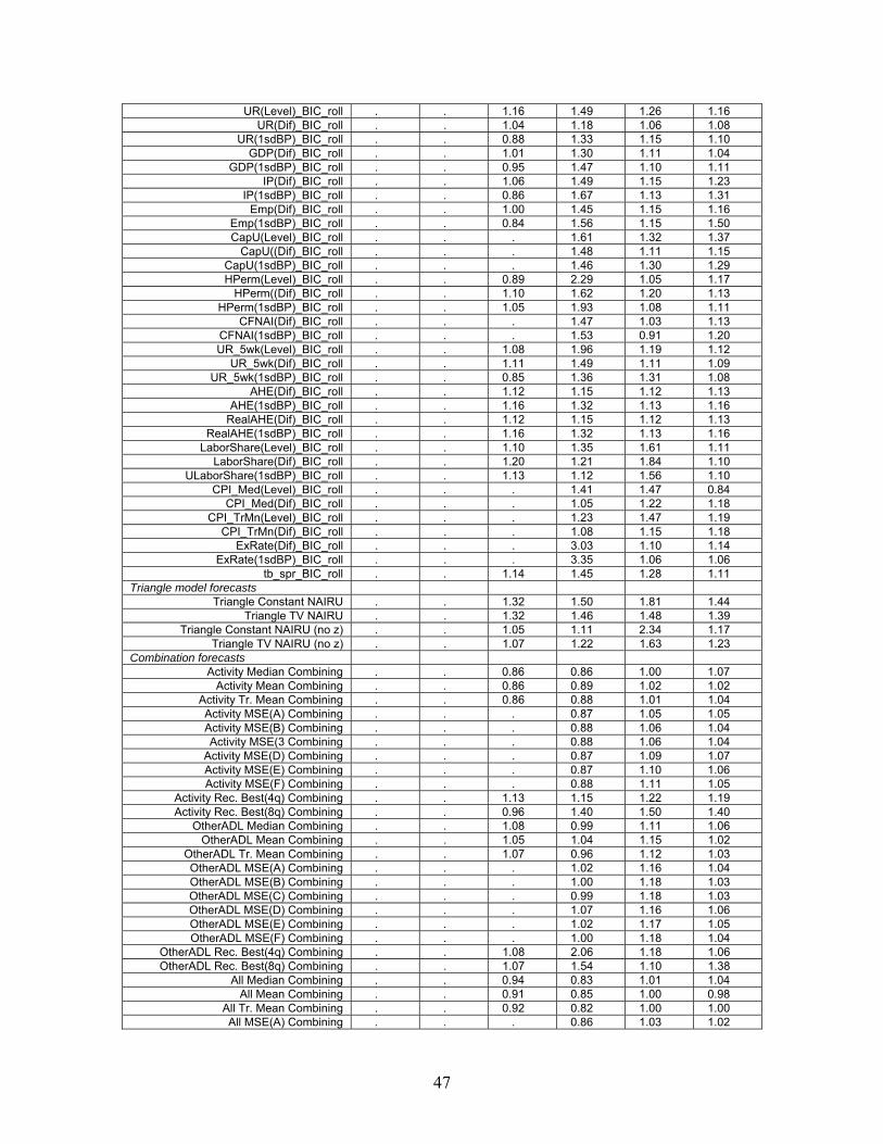
UR(Level)_BIC_roll . . 1.16 1.49 1.26 1.16 UR(Dif)_BIC_roll . . 1.04 1.18 1.06 1.08

UR(1sdBP)_BIC_roll . . 0.88 1.33 1.15 1.10 GDP(Dif)_BIC_roll . . 1.01 1.30 1.11 1.04

GDP(1sdBP)_BIC_roll . . 0.95 1.47 1.10 1.11 IP(Dif)_BIC_roll . . 1.06 1.49 1.15 1.23

IP(1sdBP)_BIC_roll . . 0.86 1.67 1.13 1.31 Emp(Dif)_BIC_roll . . 1.00 1.45 1.15 1.16

Emp(1sdBP)_BIC_roll . . 0.84 1.56 1.15 1.50 CapU(Level)_BIC_roll . . . 1.61 1.32 1.37

CapU((Dif)_BIC_roll . . . 1.48 1.11 1.15 CapU(1sdBP)_BIC_roll . . . 1.46 1.30 1.29 HPerm(Level)_BIC_roll . . 0.89 2.29 1.05 1.17

HPerm((Dif)_BIC_roll . . 1.10 1.62 1.20 1.13 HPerm(1sdBP)_BIC_roll . . 1.05 1.93 1.08 1.11

CFNAI(Dif)_BIC_roll . . . 1.47 1.03 1.13 CFNAI(1sdBP)_BIC_roll . . . 1.53 0.91 1.20 UR_5wk(Level)_BIC_roll . . 1.08 1.96 1.19 1.12

UR_5wk(Dif)_BIC_roll . . 1.11 1.49 1.11 1.09 UR_5wk(1sdBP)_BIC_roll . . 0.85 1.36 1.31 1.08

AHE(Dif)_BIC_roll . . 1.12 1.15 1.12 1.13 AHE(1sdBP)_BIC_roll . . 1.16 1.32 1.13 1.16

RealAHE(Dif)_BIC_roll . . 1.12 1.15 1.12 1.13 RealAHE(1sdBP)_BIC_roll . . 1.16 1.32 1.13 1.16

LaborShare(Level)_BIC_roll . . 1.10 1.35 1.61 1.11 LaborShare(Dif)_BIC_roll . . 1.20 1.21 1.84 1.10

ULaborShare(1sdBP)_BIC_roll . . 1.13 1.12 1.56 1.10 CPI_Med(Level)_BIC_roll . . . 1.41 1.47 0.84

CPI_Med(Dif)_BIC_roll . . . 1.05 1.22 1.18 CPI_TrMn(Level)_BIC_roll . . . 1.23 1.47 1.19

CPI_TrMn(Dif)_BIC_roll . . . 1.08 1.15 1.18 ExRate(Dif)_BIC_roll . . . 3.03 1.10 1.14

ExRate(1sdBP)_BIC_roll . . . 3.35 1.06 1.06 tb_spr_BIC_roll . . 1.14 1.45 1.28 1.11

Triangle model forecasts Triangle Constant NAIRU . . 1.32 1.50 1.81 1.44

Triangle TV NAIRU . . 1.32 1.46 1.48 1.39 Triangle Constant NAIRU (no z) . . 1.05 1.11 2.34 1.17

Triangle TV NAIRU (no z) . . 1.07 1.22 1.63 1.23 Combination forecasts

Activity Median Combining . . 0.86 0.86 1.00 1.07 Activity Mean Combining . . 0.86 0.89 1.02 1.02

Activity Tr. Mean Combining . . 0.86 0.88 1.01 1.04 Activity MSE(A) Combining . . . 0.87 1.05 1.05 Activity MSE(B) Combining . . . 0.88 1.06 1.04 Activity MSE(3 Combining . . . 0.88 1.06 1.04

Activity MSE(D) Combining . . . 0.87 1.09 1.07 Activity MSE(E) Combining . . . 0.87 1.10 1.06 Activity MSE(F) Combining . . . 0.88 1.11 1.05

Activity Rec. Best(4q) Combining . . 1.13 1.15 1.22 1.19 Activity Rec. Best(8q) Combining . . 0.96 1.40 1.50 1.40

OtherADL Median Combining . . 1.08 0.99 1.11 1.06 OtherADL Mean Combining . . 1.05 1.04 1.15 1.02

OtherADL Tr. Mean Combining . . 1.07 0.96 1.12 1.03 OtherADL MSE(A) Combining . . . 1.02 1.16 1.04 OtherADL MSE(B) Combining . . . 1.00 1.18 1.03 OtherADL MSE(C) Combining . . . 0.99 1.18 1.03 OtherADL MSE(D) Combining . . . 1.07 1.16 1.06 OtherADL MSE(E) Combining . . . 1.02 1.17 1.05 OtherADL MSE(F) Combining . . . 1.00 1.18 1.04

OtherADL Rec. Best(4q) Combining . . 1.08 2.06 1.18 1.06 OtherADL Rec. Best(8q) Combining . . 1.07 1.54 1.10 1.38

All Median Combining . . 0.94 0.83 1.01 1.04 All Mean Combining . . 0.91 0.85 1.00 0.98

All Tr. Mean Combining . . 0.92 0.82 1.00 1.00 All MSE(A) Combining . . . 0.86 1.03 1.02

47

All MSE(B) Combining . . . 0.84 1.03 1.01 All MSE(C) Combining . . . 0.84 1.02 1.01 All MSE(D) Combining . . . 0.88 1.05 1.04 All MSE(E) Combining . . . 0.85 1.05 1.03 All MSE(F) Combining . . . 0.84 1.04 1.02

All Rec. Best(4q) Combining . . 1.19 1.53 1.17 1.08 All Rec. Best(8q) Combining . . 0.96 1.67 1.45 1.50

UCSV and Triangle Rec. Best(4q) Combining

. . . 1.37 1.06 1.00

UCSV and Triangle Rec. Best(8q) Combining

. . . 1.02 1.16 1.09

48

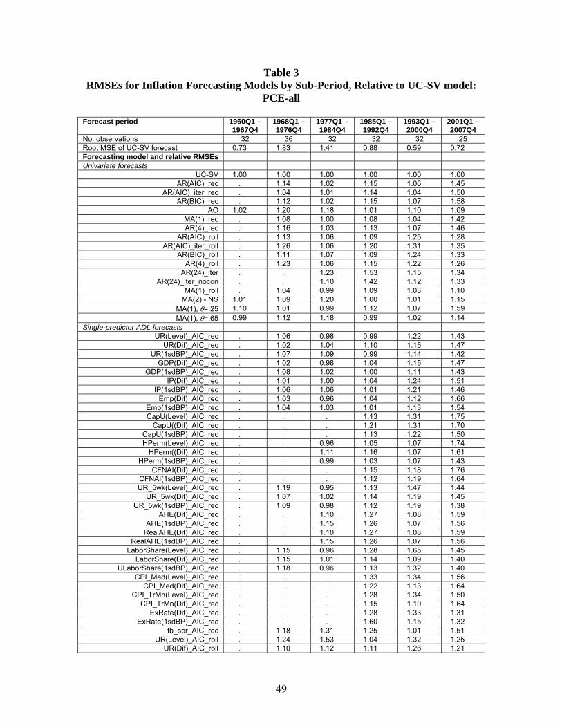
Table 3 RMSEs for Inflation Forecasting Models by Sub-Period, Relative to UC-SV model:

PCE-all Forecast period 1960Q1 –

1967Q4 1968Q1 – 1976Q4

1977Q1 - 1984Q4

1985Q1 – 1992Q4

1993Q1 – 2000Q4

2001Q1 – 2007Q4

No. observations 32 36 32 32 32 25 Root MSE of UC-SV forecast 0.73 1.83 1.41 0.88 0.59 0.72 Forecasting model and relative RMSEs Univariate forecasts

UC-SV 1.00 1.00 1.00 1.00 1.00 1.00 AR(AIC)_rec . 1.14 1.02 1.15 1.06 1.45

AR(AIC)_iter_rec . 1.04 1.01 1.14 1.04 1.50 AR(BIC)_rec . 1.12 1.02 1.15 1.07 1.58

AO 1.02 1.20 1.18 1.01 1.10 1.09 MA(1)_rec . 1.08 1.00 1.08 1.04 1.42 AR(4)_rec . 1.16 1.03 1.13 1.07 1.46

AR(AIC)_roll . 1.13 1.06 1.09 1.25 1.28 AR(AIC)_iter_roll . 1.26 1.06 1.20 1.31 1.35

AR(BIC)_roll . 1.11 1.07 1.09 1.24 1.33 AR(4)_roll . 1.23 1.06 1.15 1.22 1.26

AR(24)_iter . . 1.23 1.53 1.15 1.34 AR(24)_iter_nocon . . 1.10 1.42 1.12 1.33

MA(1)_roll . 1.04 0.99 1.09 1.03 1.10 MA(2) - NS 1.01 1.09 1.20 1.00 1.01 1.15

MA(1), θ=.25 1.10 1.01 0.99 1.12 1.07 1.59 MA(1), θ=.65 0.99 1.12 1.18 0.99 1.02 1.14

Single-predictor ADL forecasts UR(Level)_AIC_rec . 1.06 0.98 0.99 1.22 1.43

UR(Dif)_AIC_rec . 1.02 1.04 1.10 1.15 1.47 UR(1sdBP)_AIC_rec . 1.07 1.09 0.99 1.14 1.42

GDP(Dif)_AIC_rec . 1.02 0.98 1.04 1.15 1.47 GDP(1sdBP)_AIC_rec . 1.08 1.02 1.00 1.11 1.43

IP(Dif)_AIC_rec . 1.01 1.00 1.04 1.24 1.51 IP(1sdBP)_AIC_rec . 1.06 1.06 1.01 1.21 1.46

Emp(Dif)_AIC_rec . 1.03 0.96 1.04 1.12 1.66 Emp(1sdBP)_AIC_rec . 1.04 1.03 1.01 1.13 1.54 CapU(Level)_AIC_rec . . . 1.13 1.31 1.75

CapU((Dif)_AIC_rec . . . 1.21 1.31 1.70 CapU(1sdBP)_AIC_rec . . . 1.13 1.22 1.50 HPerm(Level)_AIC_rec . . 0.96 1.05 1.07 1.74

HPerm((Dif)_AIC_rec . . 1.11 1.16 1.07 1.61 HPerm(1sdBP)_AIC_rec . . 0.99 1.03 1.07 1.43

CFNAI(Dif)_AIC_rec . . . 1.15 1.18 1.76 CFNAI(1sdBP)_AIC_rec . . . 1.12 1.19 1.64 UR_5wk(Level)_AIC_rec . 1.19 0.95 1.13 1.47 1.44

UR_5wk(Dif)_AIC_rec . 1.07 1.02 1.14 1.19 1.45 UR_5wk(1sdBP)_AIC_rec . 1.09 0.98 1.12 1.19 1.38

AHE(Dif)_AIC_rec . . 1.10 1.27 1.08 1.59 AHE(1sdBP)_AIC_rec . . 1.15 1.26 1.07 1.56

RealAHE(Dif)_AIC_rec . . 1.10 1.27 1.08 1.59 RealAHE(1sdBP)_AIC_rec . . 1.15 1.26 1.07 1.56

LaborShare(Level)_AIC_rec . 1.15 0.96 1.28 1.65 1.45 LaborShare(Dif)_AIC_rec . 1.15 1.01 1.14 1.09 1.40

ULaborShare(1sdBP)_AIC_rec . 1.18 0.96 1.13 1.32 1.40 CPI_Med(Level)_AIC_rec . . . 1.33 1.34 1.56

CPI_Med(Dif)_AIC_rec . . . 1.22 1.13 1.64 CPI_TrMn(Level)_AIC_rec . . . 1.28 1.34 1.50

CPI_TrMn(Dif)_AIC_rec . . . 1.15 1.10 1.64 ExRate(Dif)_AIC_rec . . . 1.28 1.33 1.31

ExRate(1sdBP)_AIC_rec . . . 1.60 1.15 1.32 tb_spr_AIC_rec . 1.18 1.31 1.25 1.01 1.51

UR(Level)_AIC_roll . 1.24 1.53 1.04 1.32 1.25 UR(Dif)_AIC_roll . 1.10 1.12 1.11 1.26 1.21

49

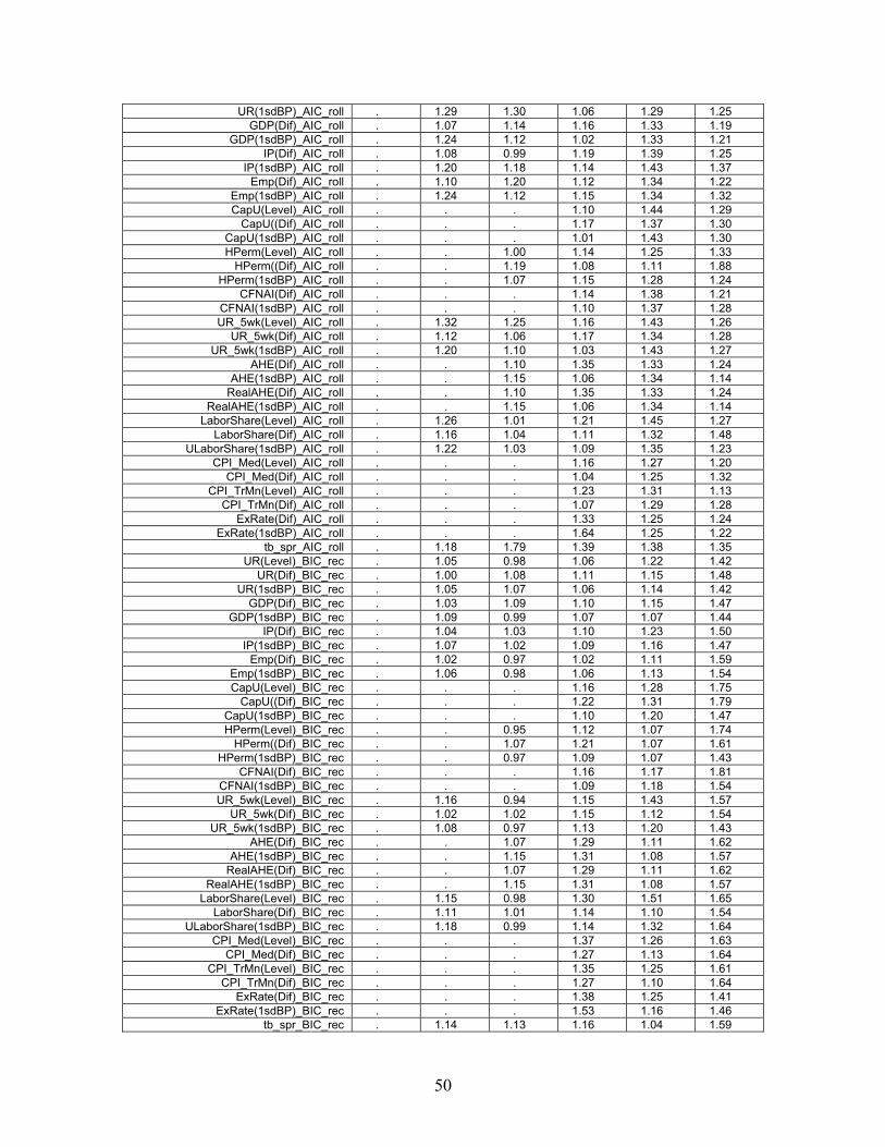
UR(1sdBP)_AIC_roll . 1.29 1.30 1.06 1.29 1.25 GDP(Dif)_AIC_roll . 1.07 1.14 1.16 1.33 1.19

GDP(1sdBP)_AIC_roll . 1.24 1.12 1.02 1.33 1.21 IP(Dif)_AIC_roll . 1.08 0.99 1.19 1.39 1.25

IP(1sdBP)_AIC_roll . 1.20 1.18 1.14 1.43 1.37 Emp(Dif)_AIC_roll . 1.10 1.20 1.12 1.34 1.22

Emp(1sdBP)_AIC_roll . 1.24 1.12 1.15 1.34 1.32 CapU(Level)_AIC_roll . . . 1.10 1.44 1.29

CapU((Dif)_AIC_roll . . . 1.17 1.37 1.30 CapU(1sdBP)_AIC_roll . . . 1.01 1.43 1.30 HPerm(Level)_AIC_roll . . 1.00 1.14 1.25 1.33

HPerm((Dif)_AIC_roll . . 1.19 1.08 1.11 1.88 HPerm(1sdBP)_AIC_roll . . 1.07 1.15 1.28 1.24

CFNAI(Dif)_AIC_roll . . . 1.14 1.38 1.21 CFNAI(1sdBP)_AIC_roll . . . 1.10 1.37 1.28 UR_5wk(Level)_AIC_roll . 1.32 1.25 1.16 1.43 1.26

UR_5wk(Dif)_AIC_roll . 1.12 1.06 1.17 1.34 1.28 UR_5wk(1sdBP)_AIC_roll . 1.20 1.10 1.03 1.43 1.27

AHE(Dif)_AIC_roll . . 1.10 1.35 1.33 1.24 AHE(1sdBP)_AIC_roll . . 1.15 1.06 1.34 1.14

RealAHE(Dif)_AIC_roll . . 1.10 1.35 1.33 1.24 RealAHE(1sdBP)_AIC_roll . . 1.15 1.06 1.34 1.14

LaborShare(Level)_AIC_roll . 1.26 1.01 1.21 1.45 1.27 LaborShare(Dif)_AIC_roll . 1.16 1.04 1.11 1.32 1.48

ULaborShare(1sdBP)_AIC_roll . 1.22 1.03 1.09 1.35 1.23 CPI_Med(Level)_AIC_roll . . . 1.16 1.27 1.20

CPI_Med(Dif)_AIC_roll . . . 1.04 1.25 1.32 CPI_TrMn(Level)_AIC_roll . . . 1.23 1.31 1.13

CPI_TrMn(Dif)_AIC_roll . . . 1.07 1.29 1.28 ExRate(Dif)_AIC_roll . . . 1.33 1.25 1.24

ExRate(1sdBP)_AIC_roll . . . 1.64 1.25 1.22 tb_spr_AIC_roll . 1.18 1.79 1.39 1.38 1.35

UR(Level)_BIC_rec . 1.05 0.98 1.06 1.22 1.42 UR(Dif)_BIC_rec . 1.00 1.08 1.11 1.15 1.48

UR(1sdBP)_BIC_rec . 1.05 1.07 1.06 1.14 1.42 GDP(Dif)_BIC_rec . 1.03 1.09 1.10 1.15 1.47

GDP(1sdBP)_BIC_rec . 1.09 0.99 1.07 1.07 1.44 IP(Dif)_BIC_rec . 1.04 1.03 1.10 1.23 1.50

IP(1sdBP)_BIC_rec . 1.07 1.02 1.09 1.16 1.47 Emp(Dif)_BIC_rec . 1.02 0.97 1.02 1.11 1.59

Emp(1sdBP)_BIC_rec . 1.06 0.98 1.06 1.13 1.54 CapU(Level)_BIC_rec . . . 1.16 1.28 1.75

CapU((Dif)_BIC_rec . . . 1.22 1.31 1.79 CapU(1sdBP)_BIC_rec . . . 1.10 1.20 1.47 HPerm(Level)_BIC_rec . . 0.95 1.12 1.07 1.74

HPerm((Dif)_BIC_rec . . 1.07 1.21 1.07 1.61 HPerm(1sdBP)_BIC_rec . . 0.97 1.09 1.07 1.43

CFNAI(Dif)_BIC_rec . . . 1.16 1.17 1.81 CFNAI(1sdBP)_BIC_rec . . . 1.09 1.18 1.54 UR_5wk(Level)_BIC_rec . 1.16 0.94 1.15 1.43 1.57

UR_5wk(Dif)_BIC_rec . 1.02 1.02 1.15 1.12 1.54 UR_5wk(1sdBP)_BIC_rec . 1.08 0.97 1.13 1.20 1.43

AHE(Dif)_BIC_rec . . 1.07 1.29 1.11 1.62 AHE(1sdBP)_BIC_rec . . 1.15 1.31 1.08 1.57

RealAHE(Dif)_BIC_rec . . 1.07 1.29 1.11 1.62 RealAHE(1sdBP)_BIC_rec . . 1.15 1.31 1.08 1.57

LaborShare(Level)_BIC_rec . 1.15 0.98 1.30 1.51 1.65 LaborShare(Dif)_BIC_rec . 1.11 1.01 1.14 1.10 1.54

ULaborShare(1sdBP)_BIC_rec . 1.18 0.99 1.14 1.32 1.64 CPI_Med(Level)_BIC_rec . . . 1.37 1.26 1.63

CPI_Med(Dif)_BIC_rec . . . 1.27 1.13 1.64 CPI_TrMn(Level)_BIC_rec . . . 1.35 1.25 1.61

CPI_TrMn(Dif)_BIC_rec . . . 1.27 1.10 1.64 ExRate(Dif)_BIC_rec . . . 1.38 1.25 1.41

ExRate(1sdBP)_BIC_rec . . . 1.53 1.16 1.46 tb_spr_BIC_rec . 1.14 1.13 1.16 1.04 1.59

50

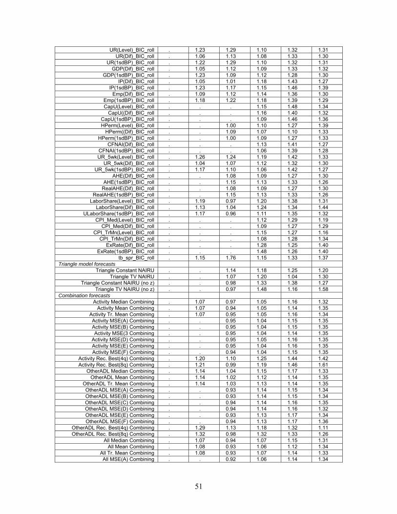
UR(Level)_BIC_roll . 1.23 1.29 1.10 1.32 1.31 UR(Dif)_BIC_roll . 1.06 1.13 1.08 1.33 1.30

UR(1sdBP)_BIC_roll . 1.22 1.29 1.10 1.32 1.31 GDP(Dif)_BIC_roll . 1.05 1.12 1.09 1.33 1.32

GDP(1sdBP)_BIC_roll . 1.23 1.09 1.12 1.28 1.30 IP(Dif)_BIC_roll . 1.05 1.01 1.18 1.43 1.27

IP(1sdBP)_BIC_roll . 1.23 1.17 1.15 1.46 1.39 Emp(Dif)_BIC_roll . 1.09 1.12 1.14 1.36 1.30

Emp(1sdBP)_BIC_roll . 1.18 1.22 1.18 1.39 1.29 CapU(Level)_BIC_roll . . . 1.15 1.48 1.34

CapU((Dif)_BIC_roll . . . 1.16 1.40 1.32 CapU(1sdBP)_BIC_roll . . . 1.09 1.46 1.36 HPerm(Level)_BIC_roll . . 1.00 1.10 1.27 1.39

HPerm((Dif)_BIC_roll . . 1.09 1.07 1.10 1.33 HPerm(1sdBP)_BIC_roll . . 1.00 1.09 1.27 1.33

CFNAI(Dif)_BIC_roll . . . 1.13 1.41 1.27 CFNAI(1sdBP)_BIC_roll . . . 1.06 1.39 1.28 UR_5wk(Level)_BIC_roll . 1.26 1.24 1.19 1.42 1.33

UR_5wk(Dif)_BIC_roll . 1.04 1.07 1.12 1.32 1.30 UR_5wk(1sdBP)_BIC_roll . 1.17 1.10 1.06 1.42 1.27

AHE(Dif)_BIC_roll . . 1.08 1.09 1.27 1.30 AHE(1sdBP)_BIC_roll . . 1.15 1.13 1.33 1.26

RealAHE(Dif)_BIC_roll . . 1.08 1.09 1.27 1.30 RealAHE(1sdBP)_BIC_roll . . 1.15 1.13 1.33 1.26

LaborShare(Level)_BIC_roll . 1.19 0.97 1.20 1.38 1.31 LaborShare(Dif)_BIC_roll . 1.13 1.04 1.24 1.34 1.44

ULaborShare(1sdBP)_BIC_roll . 1.17 0.96 1.11 1.35 1.32 CPI_Med(Level)_BIC_roll . . . 1.12 1.29 1.19

CPI_Med(Dif)_BIC_roll . . . 1.09 1.27 1.29 CPI_TrMn(Level)_BIC_roll . . . 1.15 1.27 1.16

CPI_TrMn(Dif)_BIC_roll . . . 1.08 1.28 1.34 ExRate(Dif)_BIC_roll . . . 1.28 1.25 1.40

ExRate(1sdBP)_BIC_roll . . . 1.48 1.26 1.40 tb_spr_BIC_roll . 1.15 1.76 1.15 1.33 1.37

Triangle model forecasts Triangle Constant NAIRU . . 1.14 1.18 1.25 1.20

Triangle TV NAIRU . . 1.07 1.20 1.04 1.30 Triangle Constant NAIRU (no z) . . 0.98 1.33 1.38 1.27

Triangle TV NAIRU (no z) . . 0.97 1.48 1.16 1.58 Combination forecasts

Activity Median Combining . 1.07 0.97 1.05 1.16 1.32 Activity Mean Combining . 1.07 0.94 1.05 1.14 1.35

Activity Tr. Mean Combining . 1.07 0.95 1.05 1.16 1.34 Activity MSE(A) Combining . . 0.95 1.04 1.15 1.35 Activity MSE(B) Combining . . 0.95 1.04 1.15 1.35 Activity MSE(3 Combining . . 0.95 1.04 1.14 1.35

Activity MSE(D) Combining . . 0.95 1.05 1.16 1.35 Activity MSE(E) Combining . . 0.95 1.04 1.16 1.35 Activity MSE(F) Combining . . 0.94 1.04 1.15 1.35

Activity Rec. Best(4q) Combining . 1.20 1.10 1.25 1.44 1.42 Activity Rec. Best(8q) Combining . 1.21 0.99 1.19 1.46 1.61

OtherADL Median Combining . 1.14 1.04 1.15 1.17 1.33 OtherADL Mean Combining . 1.14 1.02 1.12 1.14 1.35

OtherADL Tr. Mean Combining . 1.14 1.03 1.13 1.14 1.35 OtherADL MSE(A) Combining . . 0.93 1.14 1.15 1.34 OtherADL MSE(B) Combining . . 0.93 1.14 1.15 1.34 OtherADL MSE(C) Combining . . 0.94 1.14 1.16 1.35 OtherADL MSE(D) Combining . . 0.94 1.14 1.16 1.32 OtherADL MSE(E) Combining . . 0.93 1.13 1.17 1.34 OtherADL MSE(F) Combining . . 0.94 1.13 1.17 1.36

OtherADL Rec. Best(4q) Combining . 1.29 1.13 1.18 1.32 1.11 OtherADL Rec. Best(8q) Combining . 1.32 0.98 1.32 1.33 1.26

All Median Combining . 1.07 0.94 1.07 1.15 1.31 All Mean Combining . 1.08 0.93 1.06 1.12 1.34

All Tr. Mean Combining . 1.08 0.93 1.07 1.14 1.33 All MSE(A) Combining . . 0.92 1.06 1.14 1.34

51

All MSE(B) Combining . . 0.92 1.06 1.14 1.34 All MSE(C) Combining . . 0.92 1.06 1.13 1.34 All MSE(D) Combining . . 0.93 1.07 1.16 1.33 All MSE(E) Combining . . 0.92 1.06 1.15 1.34 All MSE(F) Combining . . 0.92 1.06 1.14 1.34

All Rec. Best(4q) Combining . 1.25 1.18 1.34 1.44 1.32 All Rec. Best(8q) Combining . 1.22 1.01 1.30 1.52 1.44

UCSV and Triangle Rec. Best(4q) Combining

. . . 1.07 1.18 1.07

UCSV and Triangle Rec. Best(8q) Combining

. . . 1.15 1.16 1.07

52

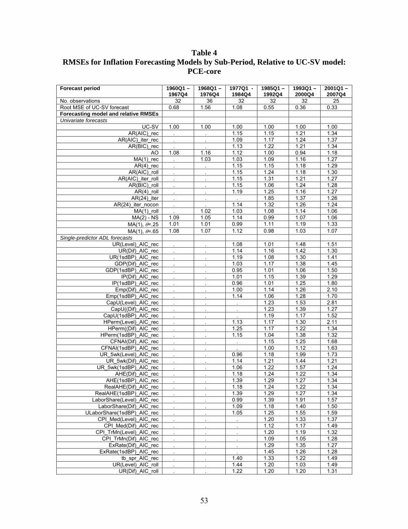
Table 4 RMSEs for Inflation Forecasting Models by Sub-Period, Relative to UC-SV model:

PCE-core Forecast period 1960Q1 –

1967Q4 1968Q1 – 1976Q4

1977Q1 - 1984Q4

1985Q1 – 1992Q4

1993Q1 – 2000Q4

2001Q1 – 2007Q4

No. observations 32 36 32 32 32 25 Root MSE of UC-SV forecast 0.68 1.56 1.08 0.55 0.36 0.33 Forecasting model and relative RMSEs Univariate forecasts

UC-SV 1.00 1.00 1.00 1.00 1.00 1.00 AR(AIC)_rec . . 1.15 1.15 1.21 1.34

AR(AIC)_iter_rec . . 1.09 1.17 1.24 1.37 AR(BIC)_rec . . 1.13 1.22 1.21 1.34

AO 1.08 1.16 1.12 1.00 0.94 1.18 MA(1)_rec . 1.03 1.03 1.09 1.16 1.27 AR(4)_rec . . 1.15 1.15 1.18 1.29

AR(AIC)_roll . . 1.15 1.24 1.18 1.30 AR(AIC)_iter_roll . . 1.15 1.31 1.21 1.27

AR(BIC)_roll . . 1.15 1.06 1.24 1.28 AR(4)_roll . . 1.19 1.25 1.16 1.27

AR(24)_iter . . . 1.85 1.37 1.26 AR(24)_iter_nocon . . 1.14 1.32 1.26 1.24

MA(1)_roll . 1.02 1.03 1.08 1.14 1.06 MA(2) - NS 1.09 1.05 1.14 0.99 1.07 1.06

MA(1), θ=.25 1.01 1.01 0.99 1.11 1.19 1.33 MA(1), θ=.65 1.08 1.07 1.12 0.98 1.03 1.07

Single-predictor ADL forecasts UR(Level)_AIC_rec . . 1.08 1.01 1.48 1.51

UR(Dif)_AIC_rec . . 1.14 1.16 1.42 1.30 UR(1sdBP)_AIC_rec . . 1.19 1.08 1.30 1.41

GDP(Dif)_AIC_rec . . 1.03 1.17 1.38 1.45 GDP(1sdBP)_AIC_rec . . 0.95 1.01 1.06 1.50

IP(Dif)_AIC_rec . . 1.01 1.15 1.39 1.29 IP(1sdBP)_AIC_rec . . 0.96 1.01 1.25 1.80

Emp(Dif)_AIC_rec . . 1.00 1.14 1.26 2.10 Emp(1sdBP)_AIC_rec . . 1.14 1.06 1.28 1.70 CapU(Level)_AIC_rec . . . 1.23 1.53 2.81

CapU((Dif)_AIC_rec . . . 1.23 1.39 1.27 CapU(1sdBP)_AIC_rec . . . 1.19 1.17 1.52 HPerm(Level)_AIC_rec . . 1.13 1.17 1.30 2.11

HPerm((Dif)_AIC_rec . . 1.25 1.17 1.22 1.34 HPerm(1sdBP)_AIC_rec . . 1.15 1.04 1.38 1.32

CFNAI(Dif)_AIC_rec . . . 1.15 1.25 1.68 CFNAI(1sdBP)_AIC_rec . . . 1.00 1.12 1.63 UR_5wk(Level)_AIC_rec . . 0.96 1.18 1.99 1.73

UR_5wk(Dif)_AIC_rec . . 1.14 1.21 1.44 1.21 UR_5wk(1sdBP)_AIC_rec . . 1.06 1.22 1.57 1.24

AHE(Dif)_AIC_rec . . 1.18 1.24 1.22 1.34 AHE(1sdBP)_AIC_rec . . 1.39 1.29 1.27 1.34

RealAHE(Dif)_AIC_rec . . 1.18 1.24 1.22 1.34 RealAHE(1sdBP)_AIC_rec . . 1.39 1.29 1.27 1.34

LaborShare(Level)_AIC_rec . . 0.99 1.39 1.91 1.57 LaborShare(Dif)_AIC_rec . . 1.09 1.18 1.40 1.50

ULaborShare(1sdBP)_AIC_rec . . 1.05 1.25 1.55 1.59 CPI_Med(Level)_AIC_rec . . . 1.20 1.33 1.37

CPI_Med(Dif)_AIC_rec . . . 1.12 1.17 1.49 CPI_TrMn(Level)_AIC_rec . . . 1.20 1.19 1.32

CPI_TrMn(Dif)_AIC_rec . . . 1.09 1.05 1.28 ExRate(Dif)_AIC_rec . . . 1.29 1.35 1.27

ExRate(1sdBP)_AIC_rec . . . 1.45 1.26 1.28 tb_spr_AIC_rec . . 1.40 1.33 1.22 1.49

UR(Level)_AIC_roll . . 1.44 1.20 1.03 1.49 UR(Dif)_AIC_roll . . 1.22 1.20 1.20 1.31

53

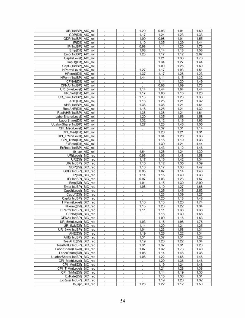
UR(1sdBP)_AIC_roll . . 1.20 0.93 1.01 1.60 GDP(Dif)_AIC_roll . . 1.17 1.24 1.23 1.33

GDP(1sdBP)_AIC_roll . . 1.00 0.98 1.01 1.55 IP(Dif)_AIC_roll . . 1.10 1.35 1.29 1.44

IP(1sdBP)_AIC_roll . . 0.98 1.11 1.20 1.73 Emp(Dif)_AIC_roll . . 1.08 1.14 1.18 1.58

Emp(1sdBP)_AIC_roll . . 1.23 1.17 1.12 2.07 CapU(Level)_AIC_roll . . . 1.21 1.33 1.73

CapU((Dif)_AIC_roll . . . 1.34 1.27 1.44 CapU(1sdBP)_AIC_roll . . . 1.00 1.26 1.60 HPerm(Level)_AIC_roll . . 1.27 1.17 1.03 1.51

HPerm((Dif)_AIC_roll . . 1.37 1.17 1.26 1.23 HPerm(1sdBP)_AIC_roll . . 1.44 1.11 1.15 1.32

CFNAI(Dif)_AIC_roll . . . 1.14 1.20 1.49 CFNAI(1sdBP)_AIC_roll . . . 0.96 1.09 1.73 UR_5wk(Level)_AIC_roll . . 1.14 1.44 1.04 1.44

UR_5wk(Dif)_AIC_roll . . 1.17 1.06 1.16 1.28 UR_5wk(1sdBP)_AIC_roll . . 1.13 1.00 1.26 1.33

AHE(Dif)_AIC_roll . . 1.18 1.25 1.21 1.32 AHE(1sdBP)_AIC_roll . . 1.36 1.36 1.21 1.61

RealAHE(Dif)_AIC_roll . . 1.18 1.25 1.21 1.32 RealAHE(1sdBP)_AIC_roll . . 1.36 1.36 1.21 1.61

LaborShare(Level)_AIC_roll . . 1.20 1.35 1.56 1.58 LaborShare(Dif)_AIC_roll . . 1.32 1.12 1.16 1.63

ULaborShare(1sdBP)_AIC_roll . . 1.27 1.23 1.46 1.55 CPI_Med(Level)_AIC_roll . . . 1.37 1.31 1.14

CPI_Med(Dif)_AIC_roll . . . 1.20 1.21 1.31 CPI_TrMn(Level)_AIC_roll . . . 1.34 1.28 1.33

CPI_TrMn(Dif)_AIC_roll . . . 1.15 1.19 1.33 ExRate(Dif)_AIC_roll . . . 1.39 1.21 1.44

ExRate(1sdBP)_AIC_roll . . . 1.43 1.12 1.46 tb_spr_AIC_roll . . 1.64 1.26 1.24 1.30

UR(Level)_BIC_rec . . 0.96 1.06 1.48 1.58 UR(Dif)_BIC_rec . . 1.17 1.16 1.42 1.34

UR(1sdBP)_BIC_rec . . 1.10 1.12 1.35 1.39 GDP(Dif)_BIC_rec . . 1.10 1.17 1.38 1.47

GDP(1sdBP)_BIC_rec . . 0.95 1.07 1.14 1.46 IP(Dif)_BIC_rec . . 1.14 1.15 1.40 1.33

IP(1sdBP)_BIC_rec . . 0.97 1.03 1.23 1.67 Emp(Dif)_BIC_rec . . 1.01 1.15 1.30 2.09

Emp(1sdBP)_BIC_rec . . 1.06 1.10 1.27 1.66 CapU(Level)_BIC_rec . . . 1.25 1.45 2.53

CapU((Dif)_BIC_rec . . . 1.23 1.39 1.27 CapU(1sdBP)_BIC_rec . . . 1.20 1.18 1.48 HPerm(Level)_BIC_rec . . 1.10 1.13 1.20 1.74

HPerm((Dif)_BIC_rec . . 1.15 1.23 1.22 1.34 HPerm(1sdBP)_BIC_rec . . 1.11 1.11 1.38 1.38

CFNAI(Dif)_BIC_rec . . . 1.16 1.30 1.68 CFNAI(1sdBP)_BIC_rec . . . 1.09 1.16 1.63 UR_5wk(Level)_BIC_rec . . 1.03 1.18 1.98 1.76

UR_5wk(Dif)_BIC_rec . . 1.14 1.20 1.21 1.25 UR_5wk(1sdBP)_BIC_rec . . 1.04 1.23 1.58 1.31

AHE(Dif)_BIC_rec . . 1.19 1.26 1.22 1.34 AHE(1sdBP)_BIC_rec . . 1.31 1.37 1.31 1.28

RealAHE(Dif)_BIC_rec . . 1.19 1.26 1.22 1.34 RealAHE(1sdBP)_BIC_rec . . 1.31 1.37 1.31 1.28

LaborShare(Level)_BIC_rec . . 1.07 1.32 1.73 1.40 LaborShare(Dif)_BIC_rec . . 1.06 1.14 1.46 1.36

ULaborShare(1sdBP)_BIC_rec . . 1.08 1.22 1.66 1.46 CPI_Med(Level)_BIC_rec . . . 1.29 1.36 1.46

CPI_Med(Dif)_BIC_rec . . . 1.19 1.24 1.48 CPI_TrMn(Level)_BIC_rec . . . 1.21 1.28 1.38

CPI_TrMn(Dif)_BIC_rec . . . 1.14 1.19 1.33 ExRate(Dif)_BIC_rec . . . 1.15 1.38 1.31

ExRate(1sdBP)_BIC_rec . . . 1.19 1.26 1.32 tb_spr_BIC_rec . . 1.26 1.22 1.12 1.50

54

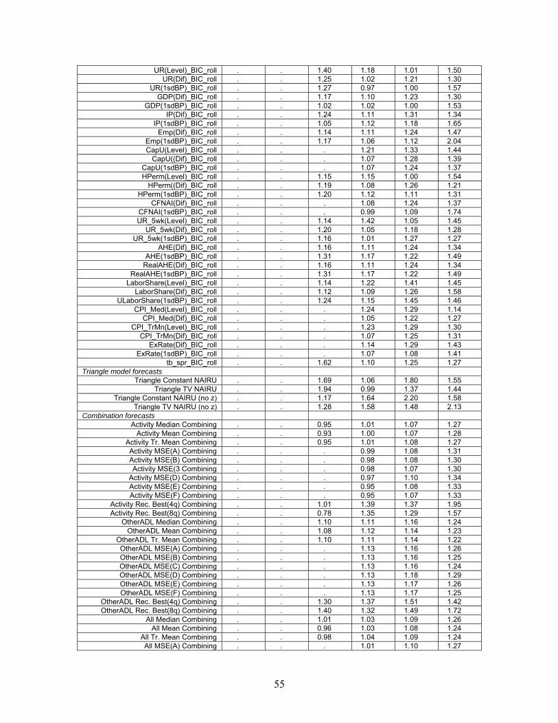
UR(Level)_BIC_roll . . 1.40 1.18 1.01 1.50 UR(Dif)_BIC_roll . . 1.25 1.02 1.21 1.30

UR(1sdBP)_BIC_roll . . 1.27 0.97 1.00 1.57 GDP(Dif)_BIC_roll . . 1.17 1.10 1.23 1.30

GDP(1sdBP)_BIC_roll . . 1.02 1.02 1.00 1.53 IP(Dif)_BIC_roll . . 1.24 1.11 1.31 1.34

IP(1sdBP)_BIC_roll . . 1.05 1.12 1.18 1.65 Emp(Dif)_BIC_roll . . 1.14 1.11 1.24 1.47

Emp(1sdBP)_BIC_roll . . 1.17 1.06 1.12 2.04 CapU(Level)_BIC_roll . . . 1.21 1.33 1.44

CapU((Dif)_BIC_roll . . . 1.07 1.28 1.39 CapU(1sdBP)_BIC_roll . . . 1.07 1.24 1.37 HPerm(Level)_BIC_roll . . 1.15 1.15 1.00 1.54

HPerm((Dif)_BIC_roll . . 1.19 1.08 1.26 1.21 HPerm(1sdBP)_BIC_roll . . 1.20 1.12 1.11 1.31

CFNAI(Dif)_BIC_roll . . . 1.08 1.24 1.37 CFNAI(1sdBP)_BIC_roll . . . 0.99 1.09 1.74 UR_5wk(Level)_BIC_roll . . 1.14 1.42 1.05 1.45

UR_5wk(Dif)_BIC_roll . . 1.20 1.05 1.18 1.28 UR_5wk(1sdBP)_BIC_roll . . 1.16 1.01 1.27 1.27

AHE(Dif)_BIC_roll . . 1.16 1.11 1.24 1.34 AHE(1sdBP)_BIC_roll . . 1.31 1.17 1.22 1.49

RealAHE(Dif)_BIC_roll . . 1.16 1.11 1.24 1.34 RealAHE(1sdBP)_BIC_roll . . 1.31 1.17 1.22 1.49

LaborShare(Level)_BIC_roll . . 1.14 1.22 1.41 1.45 LaborShare(Dif)_BIC_roll . . 1.12 1.09 1.26 1.58

ULaborShare(1sdBP)_BIC_roll . . 1.24 1.15 1.45 1.46 CPI_Med(Level)_BIC_roll . . . 1.24 1.29 1.14

CPI_Med(Dif)_BIC_roll . . . 1.05 1.22 1.27 CPI_TrMn(Level)_BIC_roll . . . 1.23 1.29 1.30

CPI_TrMn(Dif)_BIC_roll . . . 1.07 1.25 1.31 ExRate(Dif)_BIC_roll . . . 1.14 1.29 1.43

ExRate(1sdBP)_BIC_roll . . . 1.07 1.08 1.41 tb_spr_BIC_roll . . 1.62 1.10 1.25 1.27

Triangle model forecasts Triangle Constant NAIRU . . 1.69 1.06 1.80 1.55

Triangle TV NAIRU . . 1.94 0.99 1.37 1.44 Triangle Constant NAIRU (no z) . . 1.17 1.64 2.20 1.58

Triangle TV NAIRU (no z) . . 1.28 1.58 1.48 2.13 Combination forecasts

Activity Median Combining . . 0.95 1.01 1.07 1.27 Activity Mean Combining . . 0.93 1.00 1.07 1.28

Activity Tr. Mean Combining . . 0.95 1.01 1.08 1.27 Activity MSE(A) Combining . . . 0.99 1.08 1.31 Activity MSE(B) Combining . . . 0.98 1.08 1.30 Activity MSE(3 Combining . . . 0.98 1.07 1.30

Activity MSE(D) Combining . . . 0.97 1.10 1.34 Activity MSE(E) Combining . . . 0.95 1.08 1.33 Activity MSE(F) Combining . . . 0.95 1.07 1.33

Activity Rec. Best(4q) Combining . . 1.01 1.39 1.37 1.95 Activity Rec. Best(8q) Combining . . 0.78 1.35 1.29 1.57

OtherADL Median Combining . . 1.10 1.11 1.16 1.24 OtherADL Mean Combining . . 1.08 1.12 1.14 1.23

OtherADL Tr. Mean Combining . . 1.10 1.11 1.14 1.22 OtherADL MSE(A) Combining . . . 1.13 1.16 1.26 OtherADL MSE(B) Combining . . . 1.13 1.16 1.25 OtherADL MSE(C) Combining . . . 1.13 1.16 1.24 OtherADL MSE(D) Combining . . . 1.13 1.18 1.29 OtherADL MSE(E) Combining . . . 1.13 1.17 1.26 OtherADL MSE(F) Combining . . . 1.13 1.17 1.25

OtherADL Rec. Best(4q) Combining . . 1.30 1.37 1.51 1.42 OtherADL Rec. Best(8q) Combining . . 1.40 1.32 1.49 1.72

All Median Combining . . 1.01 1.03 1.09 1.26 All Mean Combining . . 0.96 1.03 1.08 1.24

All Tr. Mean Combining . . 0.98 1.04 1.09 1.24 All MSE(A) Combining . . . 1.01 1.10 1.27

55

All MSE(B) Combining . . . 1.01 1.09 1.26 All MSE(C) Combining . . . 1.00 1.08 1.26 All MSE(D) Combining . . . 1.00 1.12 1.30 All MSE(E) Combining . . . 0.98 1.10 1.29 All MSE(F) Combining . . . 0.97 1.08 1.28

All Rec. Best(4q) Combining . . 1.20 1.44 1.43 1.93 All Rec. Best(8q) Combining . . 0.78 1.35 1.43 1.61

UCSV and Triangle Rec. Best(4q) Combining

. . . 1.04 1.13 1.03

UCSV and Triangle Rec. Best(8q) Combining

. . . 1.04 1.26 1.13

56

Table 5 RMSEs for Inflation Forecasting Models by Sub-Period, Relative to UC-SV model:

GDP deflator Forecast period 1960Q1 –

1967Q4 1968Q1 – 1976Q4

1977Q1 - 1984Q4

1985Q1 – 1992Q4

1993Q1 – 2000Q4

2001Q1 – 2007Q4

No. observations 32 36 32 32 32 25 Root MSE of UC-SV forecast 0.72 1.76 1.28 0.70 0.41 0.57 Forecasting model and relative RMSEs Univariate forecasts

UC-SV 1.00 1.00 1.00 1.00 1.00 1.00 AR(AIC)_rec . 1.03 1.06 1.06 1.02 1.16

AR(AIC)_iter_rec . 1.11 1.08 1.04 0.99 1.19 AR(BIC)_rec . 1.03 1.04 1.08 1.07 1.24

AO 0.97 1.10 1.17 1.04 0.95 1.02 MA(1)_rec . 1.02 1.00 1.04 1.02 1.16 AR(4)_rec . 1.07 1.07 1.04 0.99 1.17

AR(AIC)_roll . 1.11 1.05 1.15 1.19 1.16 AR(AIC)_iter_roll . 1.10 1.06 1.02 1.12 1.11

AR(BIC)_roll . 1.08 1.05 1.21 1.17 1.11 AR(4)_roll . 1.15 1.08 1.08 1.14 1.15

AR(24)_iter . . 1.42 1.10 1.02 0.99 AR(24)_iter_nocon . . 1.34 1.02 0.99 0.99

MA(1)_roll . 1.03 0.99 1.05 0.98 1.02 MA(2) - NS 0.97 1.02 1.19 1.03 1.02 1.02

MA(1), θ=.25 1.03 1.00 1.00 1.07 1.08 1.25 MA(1), θ=.65 0.96 1.03 1.17 1.02 0.99 1.01

Single-predictor ADL forecasts UR(Level)_AIC_rec . 0.93 0.99 0.91 1.23 1.30

UR(Dif)_AIC_rec . 0.93 1.11 0.96 1.25 1.22 UR(1sdBP)_AIC_rec . 0.94 1.12 0.91 1.14 1.19

GDP(Dif)_AIC_rec . 0.94 1.04 0.91 1.06 1.09 GDP(1sdBP)_AIC_rec . 0.98 1.01 0.89 0.96 1.15

IP(Dif)_AIC_rec . 0.90 1.05 0.89 1.25 1.15 IP(1sdBP)_AIC_rec . 0.93 1.04 0.86 1.18 1.23

Emp(Dif)_AIC_rec . 0.93 1.03 0.93 1.11 1.42 Emp(1sdBP)_AIC_rec . 0.94 1.05 0.94 1.19 1.35 CapU(Level)_AIC_rec . . . 1.03 1.54 1.87

CapU((Dif)_AIC_rec . . . 0.96 1.39 1.22 CapU(1sdBP)_AIC_rec . . . 0.91 1.23 1.23 HPerm(Level)_AIC_rec . . 1.07 1.05 0.89 1.60

HPerm((Dif)_AIC_rec . . 1.17 1.09 1.01 1.13 HPerm(1sdBP)_AIC_rec . . 1.18 1.04 1.10 1.09

CFNAI(Dif)_AIC_rec . . . 1.00 1.16 1.54 CFNAI(1sdBP)_AIC_rec . . . 0.89 1.12 1.46 UR_5wk(Level)_AIC_rec . 1.08 1.01 0.92 1.83 1.32

UR_5wk(Dif)_AIC_rec . 0.99 1.07 0.93 1.32 1.11 UR_5wk(1sdBP)_AIC_rec . 0.99 1.04 0.95 1.30 1.14

AHE(Dif)_AIC_rec . . 1.09 1.09 1.05 1.16 AHE(1sdBP)_AIC_rec . . 1.21 1.19 1.07 1.13

RealAHE(Dif)_AIC_rec . . 1.09 1.09 1.05 1.16 RealAHE(1sdBP)_AIC_rec . . 1.21 1.19 1.07 1.13

LaborShare(Level)_AIC_rec . 1.10 0.99 1.18 1.85 1.27 LaborShare(Dif)_AIC_rec . 1.09 1.06 1.07 1.12 1.14

ULaborShare(1sdBP)_AIC_rec . 1.10 1.01 1.08 1.47 1.13 CPI_Med(Level)_AIC_rec . . . 1.09 1.38 1.29

CPI_Med(Dif)_AIC_rec . . . 1.02 1.15 1.34 CPI_TrMn(Level)_AIC_rec . . . 1.12 1.17 1.21

CPI_TrMn(Dif)_AIC_rec . . . 1.02 0.96 1.19 ExRate(Dif)_AIC_rec . . . 1.23 1.44 1.06

ExRate(1sdBP)_AIC_rec . . . 1.66 1.25 0.91 tb_spr_AIC_rec . 1.08 1.23 1.19 0.95 1.27

UR(Level)_AIC_roll . 1.09 1.43 1.06 1.16 1.11 UR(Dif)_AIC_roll . 0.97 1.35 1.12 1.25 1.06

57

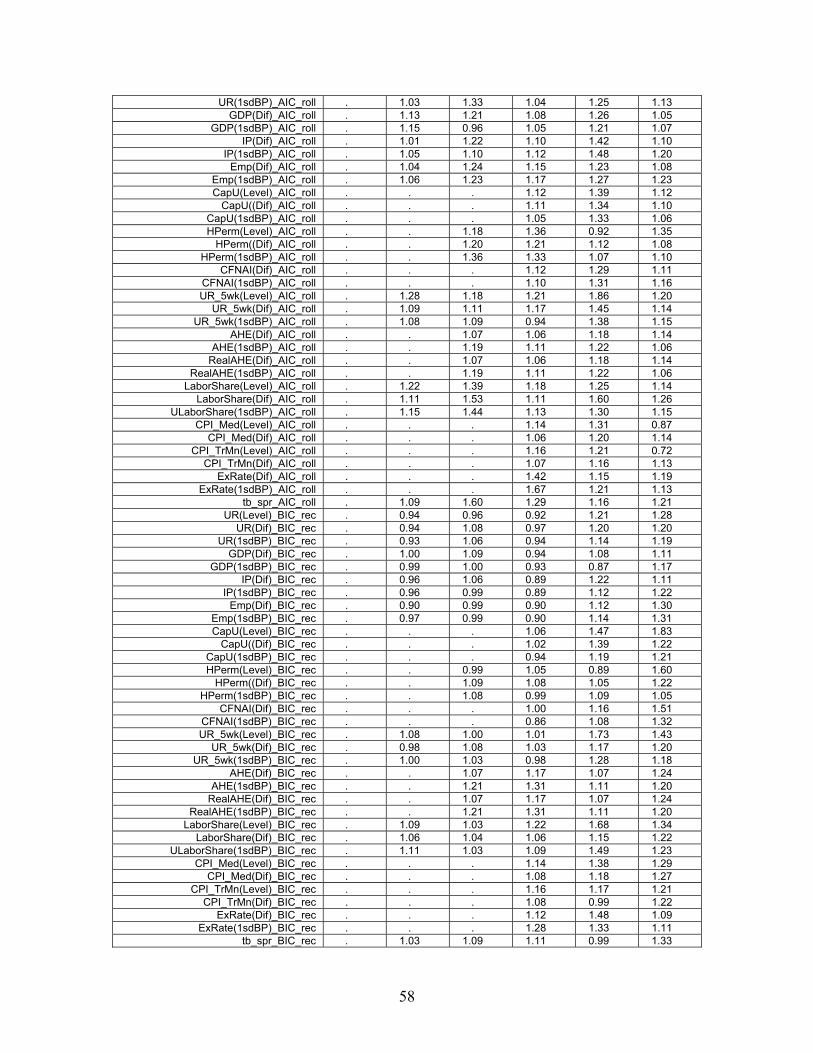
UR(1sdBP)_AIC_roll . 1.03 1.33 1.04 1.25 1.13 GDP(Dif)_AIC_roll . 1.13 1.21 1.08 1.26 1.05

GDP(1sdBP)_AIC_roll . 1.15 0.96 1.05 1.21 1.07 IP(Dif)_AIC_roll . 1.01 1.22 1.10 1.42 1.10

IP(1sdBP)_AIC_roll . 1.05 1.10 1.12 1.48 1.20 Emp(Dif)_AIC_roll . 1.04 1.24 1.15 1.23 1.08

Emp(1sdBP)_AIC_roll . 1.06 1.23 1.17 1.27 1.23 CapU(Level)_AIC_roll . . . 1.12 1.39 1.12

CapU((Dif)_AIC_roll . . . 1.11 1.34 1.10 CapU(1sdBP)_AIC_roll . . . 1.05 1.33 1.06 HPerm(Level)_AIC_roll . . 1.18 1.36 0.92 1.35

HPerm((Dif)_AIC_roll . . 1.20 1.21 1.12 1.08 HPerm(1sdBP)_AIC_roll . . 1.36 1.33 1.07 1.10

CFNAI(Dif)_AIC_roll . . . 1.12 1.29 1.11 CFNAI(1sdBP)_AIC_roll . . . 1.10 1.31 1.16 UR_5wk(Level)_AIC_roll . 1.28 1.18 1.21 1.86 1.20

UR_5wk(Dif)_AIC_roll . 1.09 1.11 1.17 1.45 1.14 UR_5wk(1sdBP)_AIC_roll . 1.08 1.09 0.94 1.38 1.15

AHE(Dif)_AIC_roll . . 1.07 1.06 1.18 1.14 AHE(1sdBP)_AIC_roll . . 1.19 1.11 1.22 1.06

RealAHE(Dif)_AIC_roll . . 1.07 1.06 1.18 1.14 RealAHE(1sdBP)_AIC_roll . . 1.19 1.11 1.22 1.06

LaborShare(Level)_AIC_roll . 1.22 1.39 1.18 1.25 1.14 LaborShare(Dif)_AIC_roll . 1.11 1.53 1.11 1.60 1.26

ULaborShare(1sdBP)_AIC_roll . 1.15 1.44 1.13 1.30 1.15 CPI_Med(Level)_AIC_roll . . . 1.14 1.31 0.87

CPI_Med(Dif)_AIC_roll . . . 1.06 1.20 1.14 CPI_TrMn(Level)_AIC_roll . . . 1.16 1.21 0.72

CPI_TrMn(Dif)_AIC_roll . . . 1.07 1.16 1.13 ExRate(Dif)_AIC_roll . . . 1.42 1.15 1.19

ExRate(1sdBP)_AIC_roll . . . 1.67 1.21 1.13 tb_spr_AIC_roll . 1.09 1.60 1.29 1.16 1.21

UR(Level)_BIC_rec . 0.94 0.96 0.92 1.21 1.28 UR(Dif)_BIC_rec . 0.94 1.08 0.97 1.20 1.20

UR(1sdBP)_BIC_rec . 0.93 1.06 0.94 1.14 1.19 GDP(Dif)_BIC_rec . 1.00 1.09 0.94 1.08 1.11

GDP(1sdBP)_BIC_rec . 0.99 1.00 0.93 0.87 1.17 IP(Dif)_BIC_rec . 0.96 1.06 0.89 1.22 1.11

IP(1sdBP)_BIC_rec . 0.96 0.99 0.89 1.12 1.22 Emp(Dif)_BIC_rec . 0.90 0.99 0.90 1.12 1.30

Emp(1sdBP)_BIC_rec . 0.97 0.99 0.90 1.14 1.31 CapU(Level)_BIC_rec . . . 1.06 1.47 1.83

CapU((Dif)_BIC_rec . . . 1.02 1.39 1.22 CapU(1sdBP)_BIC_rec . . . 0.94 1.19 1.21 HPerm(Level)_BIC_rec . . 0.99 1.05 0.89 1.60

HPerm((Dif)_BIC_rec . . 1.09 1.08 1.05 1.22 HPerm(1sdBP)_BIC_rec . . 1.08 0.99 1.09 1.05

CFNAI(Dif)_BIC_rec . . . 1.00 1.16 1.51 CFNAI(1sdBP)_BIC_rec . . . 0.86 1.08 1.32 UR_5wk(Level)_BIC_rec . 1.08 1.00 1.01 1.73 1.43

UR_5wk(Dif)_BIC_rec . 0.98 1.08 1.03 1.17 1.20 UR_5wk(1sdBP)_BIC_rec . 1.00 1.03 0.98 1.28 1.18

AHE(Dif)_BIC_rec . . 1.07 1.17 1.07 1.24 AHE(1sdBP)_BIC_rec . . 1.21 1.31 1.11 1.20

RealAHE(Dif)_BIC_rec . . 1.07 1.17 1.07 1.24 RealAHE(1sdBP)_BIC_rec . . 1.21 1.31 1.11 1.20

LaborShare(Level)_BIC_rec . 1.09 1.03 1.22 1.68 1.34 LaborShare(Dif)_BIC_rec . 1.06 1.04 1.06 1.15 1.22

ULaborShare(1sdBP)_BIC_rec . 1.11 1.03 1.09 1.49 1.23 CPI_Med(Level)_BIC_rec . . . 1.14 1.38 1.29

CPI_Med(Dif)_BIC_rec . . . 1.08 1.18 1.27 CPI_TrMn(Level)_BIC_rec . . . 1.16 1.17 1.21

CPI_TrMn(Dif)_BIC_rec . . . 1.08 0.99 1.22 ExRate(Dif)_BIC_rec . . . 1.12 1.48 1.09

ExRate(1sdBP)_BIC_rec . . . 1.28 1.33 1.11 tb_spr_BIC_rec . 1.03 1.09 1.11 0.99 1.33

58

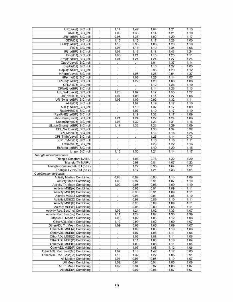
UR(Level)_BIC_roll . 1.14 1.49 1.04 1.21 1.15 UR(Dif)_BIC_roll . 1.03 1.33 1.14 1.21 1.10

UR(1sdBP)_BIC_roll . 0.98 1.36 1.02 1.20 1.17 GDP(Dif)_BIC_roll . 1.15 1.15 1.17 1.28 1.00

GDP(1sdBP)_BIC_roll . 1.15 0.98 1.06 1.20 1.10 IP(Dif)_BIC_roll . 1.05 1.16 1.10 1.34 1.08

IP(1sdBP)_BIC_roll . 1.09 1.13 1.18 1.43 1.24 Emp(Dif)_BIC_roll . 1.03 1.21 1.15 1.25 1.11

Emp(1sdBP)_BIC_roll . 1.04 1.24 1.24 1.27 1.24 CapU(Level)_BIC_roll . . . 1.01 1.37 1.14

CapU((Dif)_BIC_roll . . . 1.10 1.27 1.05 CapU(1sdBP)_BIC_roll . . . 0.96 1.29 1.12 HPerm(Level)_BIC_roll . . 1.08 1.25 0.94 1.37

HPerm((Dif)_BIC_roll . . 1.08 1.25 1.14 1.07 HPerm(1sdBP)_BIC_roll . . 1.22 1.20 1.08 1.08

CFNAI(Dif)_BIC_roll . . . 1.12 1.28 1.10 CFNAI(1sdBP)_BIC_roll . . . 1.14 1.25 1.13 UR_5wk(Level)_BIC_roll . 1.28 1.07 1.17 1.55 1.22

UR_5wk(Dif)_BIC_roll . 1.07 1.08 1.14 1.27 1.08 UR_5wk(1sdBP)_BIC_roll . 1.06 1.09 0.93 1.32 1.11

AHE(Dif)_BIC_roll . . 1.07 1.19 1.17 1.10 AHE(1sdBP)_BIC_roll . . 1.19 1.32 1.17 1.09

RealAHE(Dif)_BIC_roll . . 1.07 1.19 1.17 1.10 RealAHE(1sdBP)_BIC_roll . . 1.19 1.32 1.17 1.09

LaborShare(Level)_BIC_roll . 1.21 1.24 1.22 1.24 1.06 LaborShare(Dif)_BIC_roll . 1.06 1.32 1.23 1.31 1.16

ULaborShare(1sdBP)_BIC_roll . 1.17 1.32 1.23 1.29 1.09 CPI_Med(Level)_BIC_roll . . . 1.36 1.34 0.92

CPI_Med(Dif)_BIC_roll . . . 1.13 1.18 1.26 CPI_TrMn(Level)_BIC_roll . . . 1.26 1.14 0.73

CPI_TrMn(Dif)_BIC_roll . . . 1.16 1.16 1.11 ExRate(Dif)_BIC_roll . . . 1.26 1.22 1.16

ExRate(1sdBP)_BIC_roll . . . 1.49 1.20 1.15 tb_spr_BIC_roll . 1.13 1.50 1.21 1.14 1.17

Triangle model forecasts Triangle Constant NAIRU . . 1.08 0.78 1.22 1.20

Triangle TV NAIRU . . 0.98 0.81 1.07 1.23 Triangle Constant NAIRU (no z) . . 1.22 0.95 1.64 1.22

Triangle TV NAIRU (no z) . . 1.17 1.21 1.33 1.61 Combination forecasts

Activity Median Combining . 0.98 0.99 0.93 1.10 1.09 Activity Mean Combining . 1.00 0.97 0.91 1.07 1.10

Activity Tr. Mean Combining . 1.00 0.98 0.93 1.09 1.10 Activity MSE(A) Combining . . 0.98 0.91 1.09 1.11 Activity MSE(B) Combining . . 0.98 0.91 1.09 1.11 Activity MSE(3 Combining . . 0.98 0.91 1.08 1.10

Activity MSE(D) Combining . . 0.98 0.89 1.10 1.11 Activity MSE(E) Combining . . 0.98 0.89 1.09 1.11 Activity MSE(F) Combining . . 0.98 0.89 1.08 1.11

Activity Rec. Best(4q) Combining . 1.09 1.24 1.02 1.33 1.07 Activity Rec. Best(8q) Combining . 1.11 1.29 1.02 1.30 1.39

OtherADL Median Combining . 1.09 1.02 1.06 1.12 1.08 OtherADL Mean Combining . 1.10 0.99 1.02 1.09 1.07

OtherADL Tr. Mean Combining . 1.09 0.98 1.05 1.09 1.07 OtherADL MSE(A) Combining . . 1.09 1.08 1.10 1.06 OtherADL MSE(B) Combining . . 1.07 1.08 1.11 1.06 OtherADL MSE(C) Combining . . 1.06 1.08 1.11 1.06 OtherADL MSE(D) Combining . . 1.11 1.08 1.10 1.04 OtherADL MSE(E) Combining . . 1.09 1.08 1.11 1.04 OtherADL MSE(F) Combining . . 1.07 1.08 1.12 1.06

OtherADL Rec. Best(4q) Combining . 1.07 1.18 1.42 1.12 0.83 OtherADL Rec. Best(8q) Combining . 1.15 1.32 1.22 1.05 0.91

All Median Combining . 1.01 0.97 0.98 1.10 1.07 All Mean Combining . 1.02 0.94 0.94 1.05 1.08

All Tr. Mean Combining . 1.02 0.94 0.97 1.06 1.07 All MSE(A) Combining . . 0.97 0.95 1.07 1.07

59

All MSE(B) Combining . . 0.96 0.95 1.07 1.07 All MSE(C) Combining . . 0.96 0.95 1.07 1.07 All MSE(D) Combining . . 0.98 0.94 1.09 1.07 All MSE(E) Combining . . 0.98 0.93 1.09 1.07 All MSE(F) Combining . . 0.97 0.93 1.07 1.07

All Rec. Best(4q) Combining . 1.07 1.35 1.20 1.32 0.90 All Rec. Best(8q) Combining . 1.12 1.37 1.03 1.16 1.03

UCSV and Triangle Rec. Best(4q) Combining

. . . 0.91 1.14 1.17

UCSV and Triangle Rec. Best(8q) Combining

. . . 0.89 1.13 1.21

60

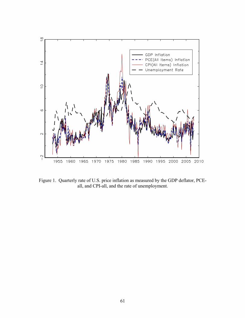
Figure 1. Quarterly rate of U.S. price inflation as measured by the GDP deflator, PCE-all, and CPI-all, and the rate of unemployment.

61

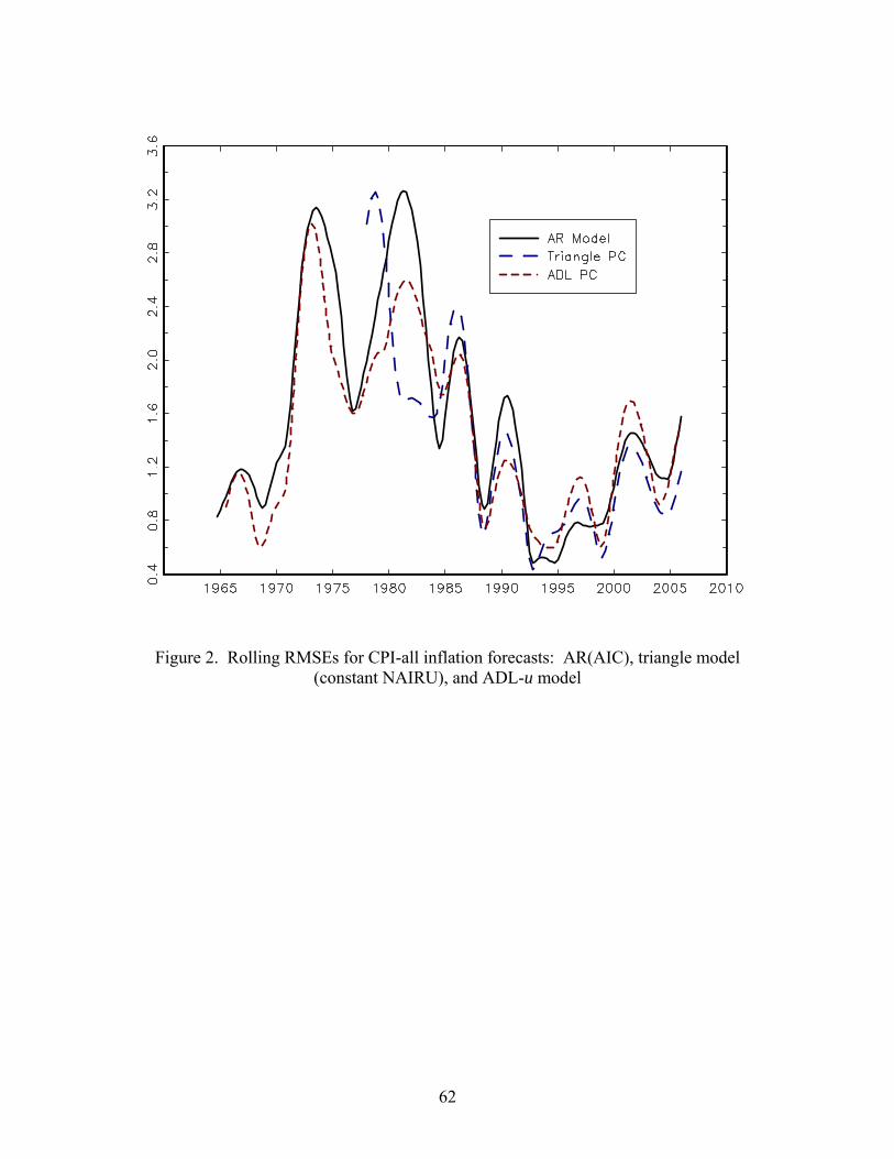
Figure 2. Rolling RMSEs for CPI-all inflation forecasts: AR(AIC), triangle model (constant NAIRU), and ADL-u model

62

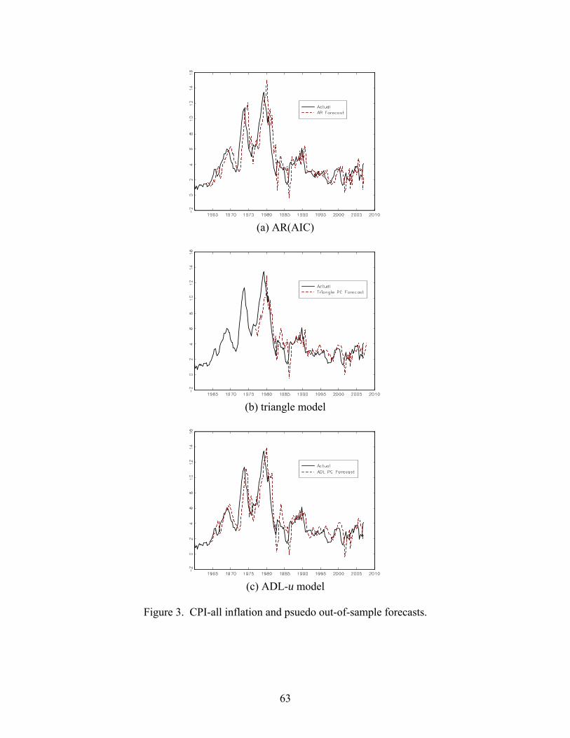
(a) AR(AIC)

(b) triangle model

(c) ADL-u model

Figure 3. CPI-all inflation and psuedo out-of-sample forecasts.

63

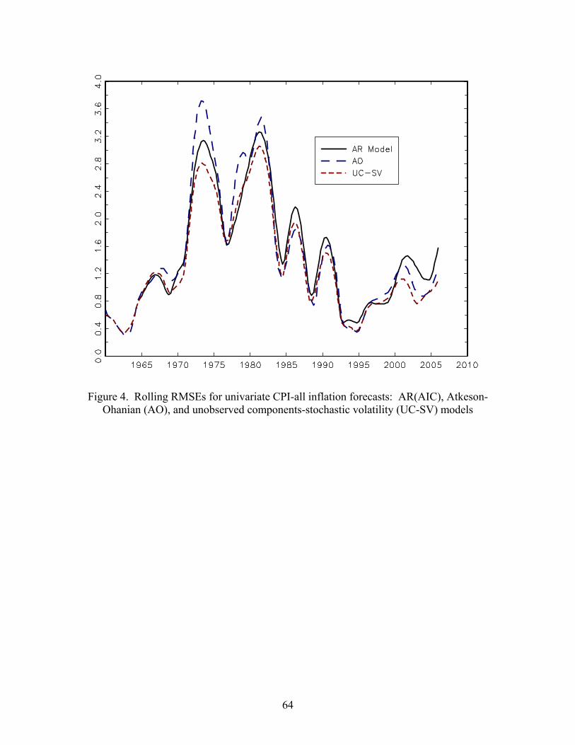
Figure 4. Rolling RMSEs for univariate CPI-all inflation forecasts: AR(AIC), Atkeson-Ohanian (AO), and unobserved components-stochastic volatility (UC-SV) models

64

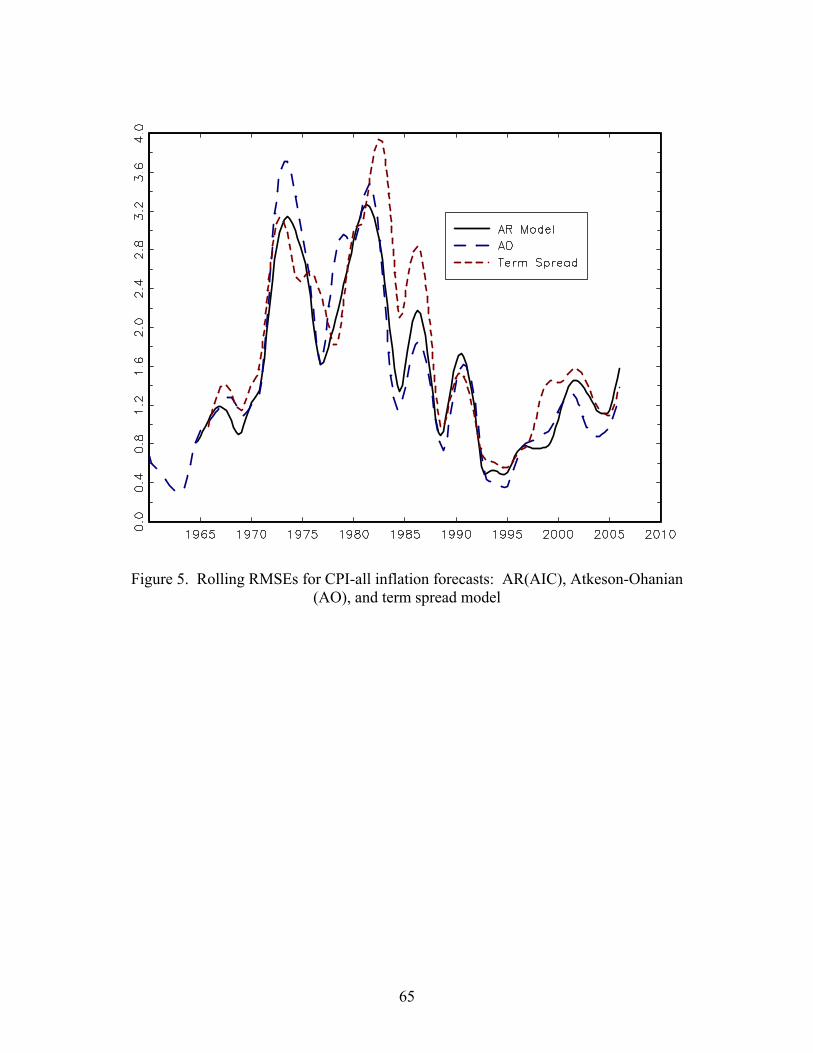
Figure 5. Rolling RMSEs for CPI-all inflation forecasts: AR(AIC), Atkeson-Ohanian (AO), and term spread model

65

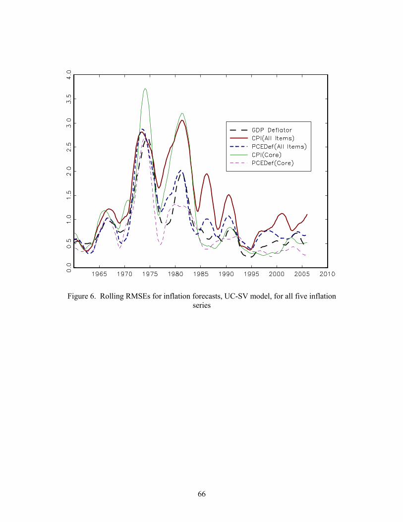
Figure 6. Rolling RMSEs for inflation forecasts, UC-SV model, for all five inflation series

66

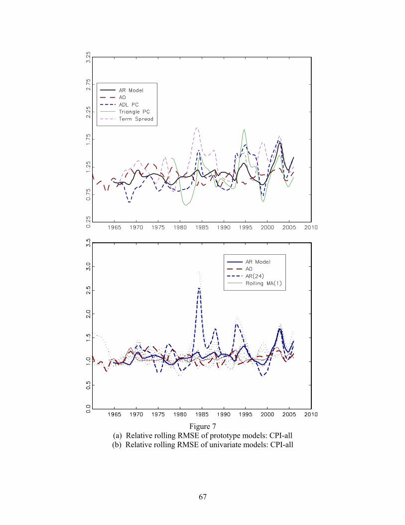
Figure 7

(a) Relative rolling RMSE of prototype models: CPI-all (b) Relative rolling RMSE of univariate models: CPI-all

67

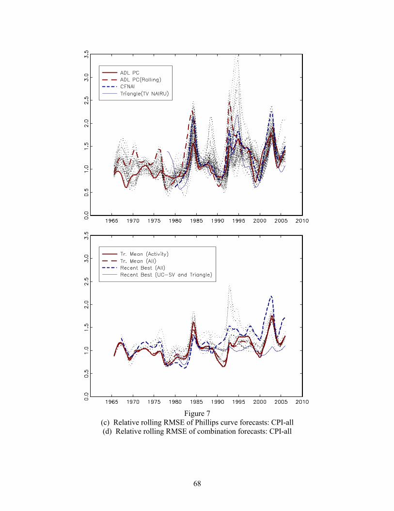
Figure 7

(c) Relative rolling RMSE of Phillips curve forecasts: CPI-all (d) Relative rolling RMSE of combination forecasts: CPI-all

68

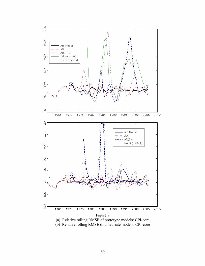
Figure 8

(a) Relative rolling RMSE of prototype models: CPI-core (b) Relative rolling RMSE of univariate models: CPI-core

69

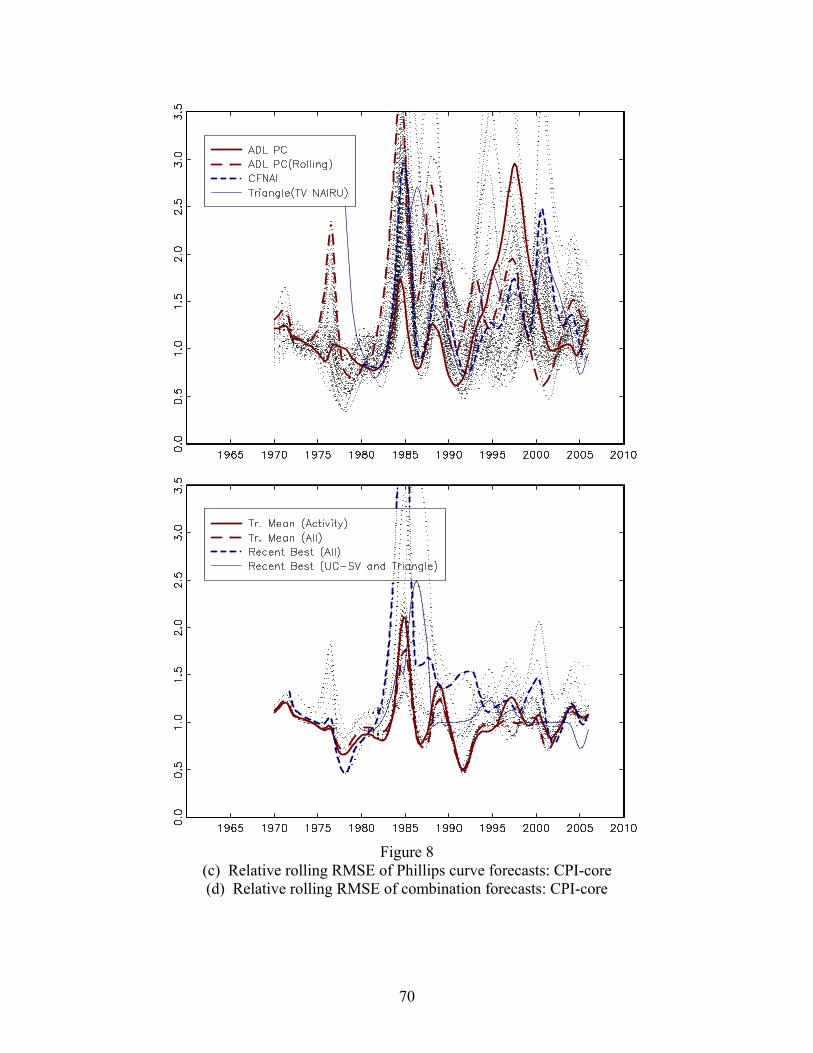
Figure 8

(c) Relative rolling RMSE of Phillips curve forecasts: CPI-core (d) Relative rolling RMSE of combination forecasts: CPI-core

70

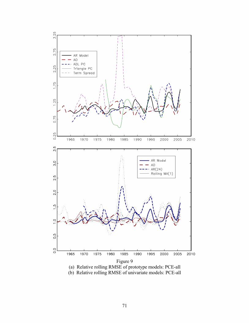
Figure 9

(a) Relative rolling RMSE of prototype models: PCE-all (b) Relative rolling RMSE of univariate models: PCE-all

71

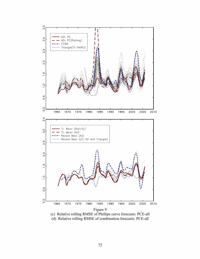
Figure 9

(c) Relative rolling RMSE of Phillips curve forecasts: PCE-all (d) Relative rolling RMSE of combination forecasts: PCE-all

72

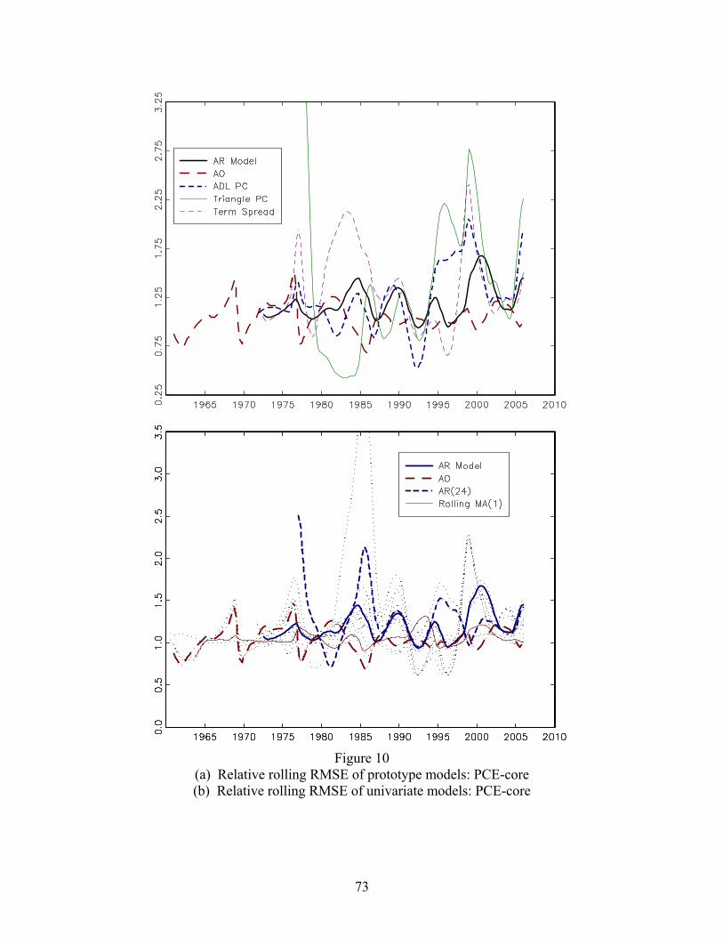
Figure 10

(a) Relative rolling RMSE of prototype models: PCE-core (b) Relative rolling RMSE of univariate models: PCE-core

73

Figure 10

(c) Relative rolling RMSE of Phillips curve forecasts: PCE-core (d) Relative rolling RMSE of combination forecasts: PCE-core

74

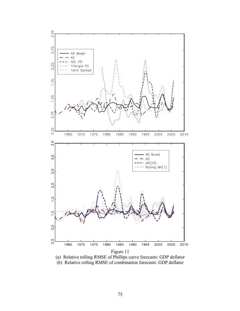
Figure 11

(a) Relative rolling RMSE of Phillips curve forecasts: GDP deflator (b) Relative rolling RMSE of combination forecasts: GDP deflator

75

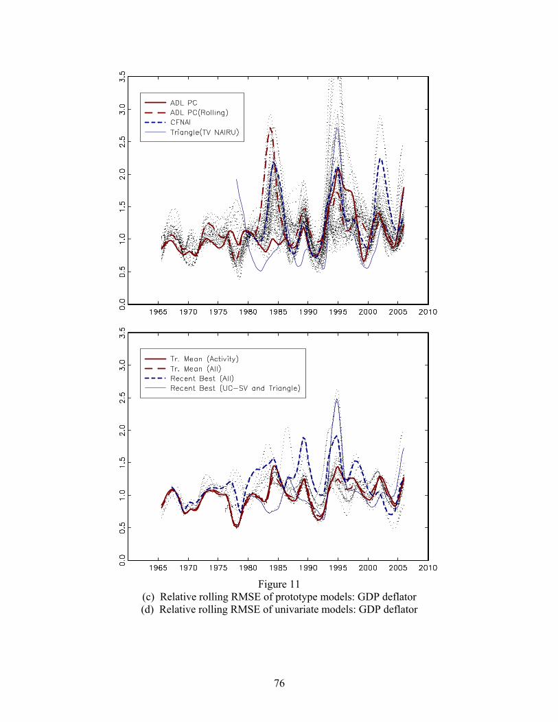
Figure 11

(c) Relative rolling RMSE of prototype models: GDP deflator (d) Relative rolling RMSE of univariate models: GDP deflator

76

Figure 12. RMSEs of headline inflation forecasts, relative to UC-SV, for (a) triangle

model and (b) ADL-u model. The unemployment rate is plotted in (c).

77

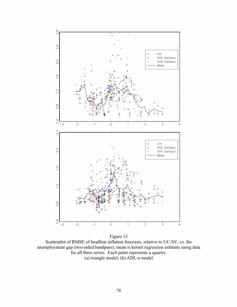
Figure 13 Scatterplot of RMSE of headline inflation forecasts, relative to UC-SV, vs. the

unemployment gap (two-sided bandpass); mean is kernel regression estimate using data for all three series. Each point represents a quarter.

(a) triangle model; (b) ADL-u model

78

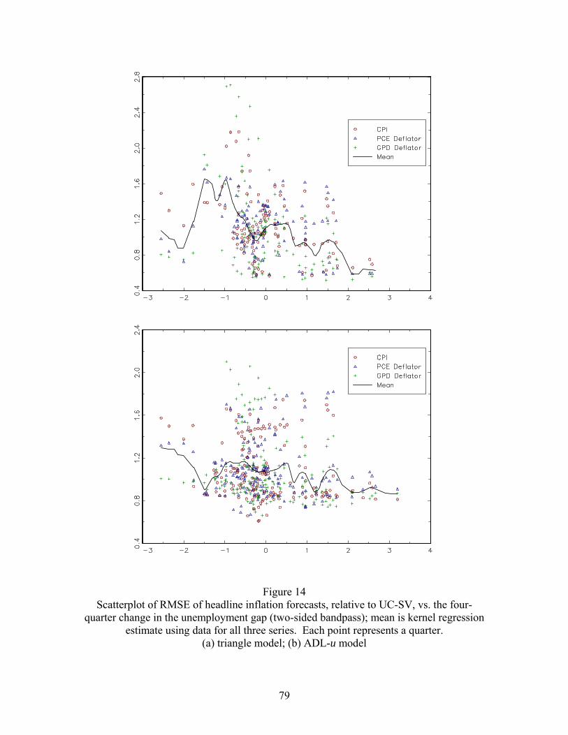
Figure 14 Scatterplot of RMSE of headline inflation forecasts, relative to UC-SV, vs. the four-

quarter change in the unemployment gap (two-sided bandpass); mean is kernel regression estimate using data for all three series. Each point represents a quarter.

(a) triangle model; (b) ADL-u model

79

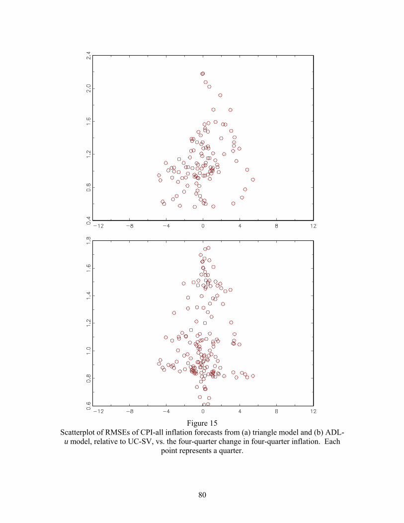
Figure 15

Scatterplot of RMSEs of CPI-all inflation forecasts from (a) triangle model and (b) ADL-u model, relative to UC-SV, vs. the four-quarter change in four-quarter inflation. Each

point represents a quarter.

80

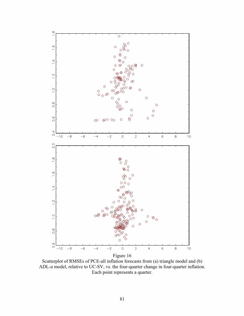
Figure 16

Scatterplot of RMSEs of PCE-all inflation forecasts from (a) triangle model and (b) ADL-u model, relative to UC-SV, vs. the four-quarter change in four-quarter inflation.

Each point represents a quarter.

81

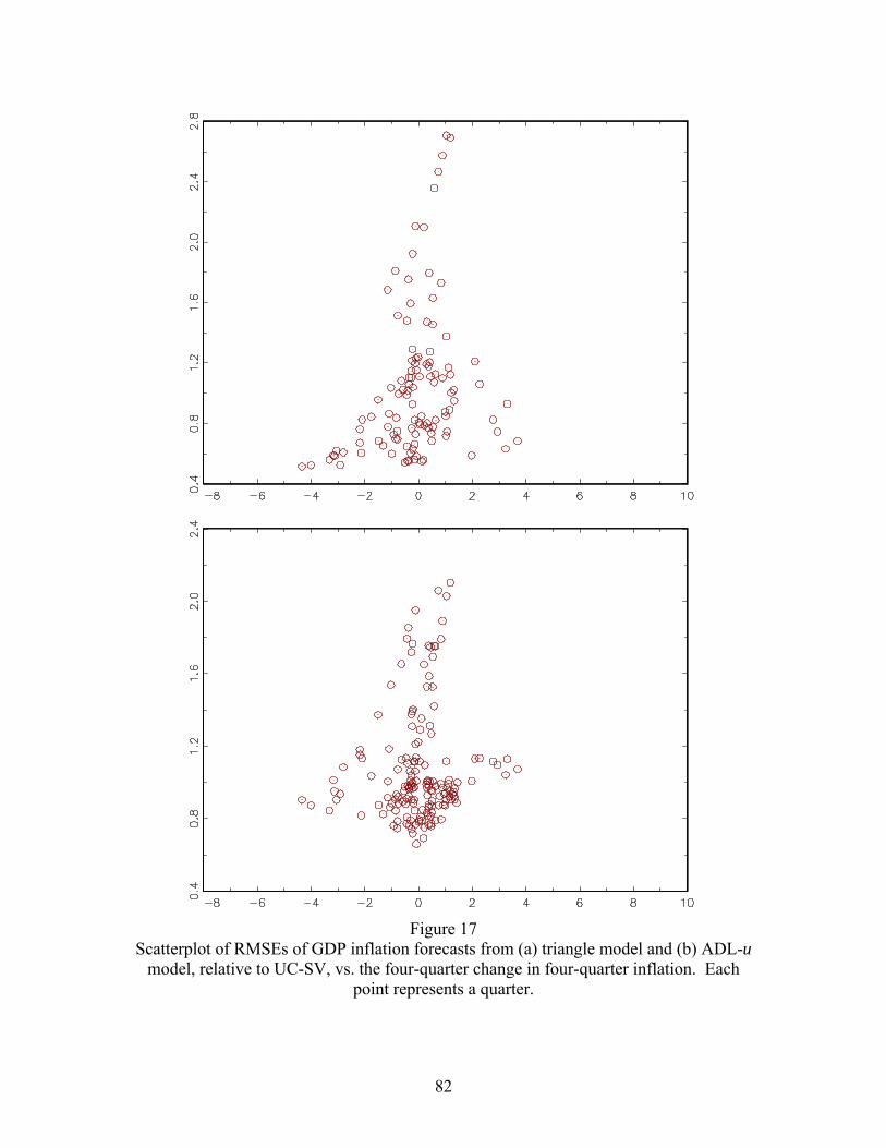
Figure 17

Scatterplot of RMSEs of GDP inflation forecasts from (a) triangle model and (b) ADL-u model, relative to UC-SV, vs. the four-quarter change in four-quarter inflation. Each

point represents a quarter.

82