Rothko Research | Empirical Analysis

Phillips Curve and

Wage Inflation Dynamics

Abstract: Debates around the Phillips curve, a long-time relationship between unemployment and

wage inflation, have been haunting both academics and practitioners over the past few years. Despite

unemployment rate at its lowest level in decades, wage growth has been weak in most of the

developed countries. There can be various factors that may be playing a part, ranging from a collapse

in the rate of union membership for private-sector employees to a higher concentration of large firms

(employers have become monopsonists, impacting level of wages). Therefore, in this article, we

review the development of the Phillips Curves in the major development economies and look at the

short-run and long-run determinants of wage inflation according to recent empirical research.

Rothko Research | Empirical Analysis

I. Is the Phillips Curve dead?

Many observers have argued in the recent years that the Phillips curve has flattened in most of the

developed nations. In this section, we look at the behaviour of the curve in 7 advanced economies –

US, UK, Japan, France, Germany, Italy, Spain - to see if we can confirm the latest statement. We use

AMECO database, an annual macro-economic database of the European Commission, which runs from

1960 to 2018 (projections for the year 2018). For the wage inflation, we calculate the year-on-year

growth of the compensation of employees (total economy) that we get in the labour costs file (see

data attached).

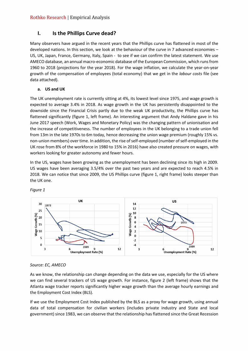
a. US and UK

The UK unemployment rate is currently sitting at 4%, its lowest level since 1975, and wage growth is

expected to average 3.4% in 2018. As wage growth in the UK has persistently disappointed to the

downside since the Financial Crisis partly due to the weak UK productivity, the Phillips curve has

flattened significantly (figure 1, left frame). An interesting argument that Andy Haldane gave in his

June 2017 speech (Work, Wages and Monetary Policy) was the changing pattern of unionisation and

the increase of competitiveness. The number of employees in the UK belonging to a trade union fell

from 13m in the late 1970s to 6m today, hence decreasing the union wage premium (roughly 15% vs.

non-union members) over time. In addition, the rise of self-employed (number of self-employed in the

UK rose from 8% of the workforce in 1980 to 15% in 2016) have also created pressure on wages, with

workers looking for greater autonomy and fewer hours.

In the US, wages have been growing as the unemployment has been declining since its high in 2009.

US wages have been averaging 3.5/4% over the past two years and are expected to reach 4.5% in

2018. We can notice that since 2009, the US Phillips curve (figure 1, right frame) looks steeper than

the UK one.

Figure 1

Source: EC, AMECO

As we know, the relationship can change depending on the data we use, especially for the US where

we can find several trackers of US wage growth. For instance, figure 2 (left frame) shows that the

Atlanta wage tracker reports significantly higher wage growth than the average hourly earnings and

the Employment Cost Index (BLS).

If we use the Employment Cost Index published by the BLS as a proxy for wage growth, using annual

data of total compensation for civilian workers (includes private industry and State and local

government) since 1983, we can observe that the relationship has flattened since the Great Recession

Rothko Research | Empirical Analysis

(figure 2, right frame). While the unemployment rate halved between 2009 and 2015, wage inflation

remained steady at 2%.

Figure 2

Source: Atlanta Fed, Fred, Eikon Reuters

b. Euro area

1. Germany

In Germany, we can notice that the Phillips has certainly flattened since the turn of the century,

however the negative relationship is still present if we look at the 2009 – 2018 window. First, German

wages growth has constantly outperformed those of the Euro area over the past 8 years. However, as

the unemployment rate fell from 6% to 3.5% between 2011 and 2018, and given the strong recovery,

wage growth has remained steady oscillating around 4%. There are several factors explaining the weak

wage growth in Germany: low inflation in 2015-2016, modest rise in productivity, strong immigration

from other countries and a high labour participation rate (relative to the Euro area). However, if the

economic outlook remains robust, labour tightness and rising inflation will be reflected to a greater

extent in actual wage development.

Figure 3

Source: EC, AMECO

Rothko Research | Empirical Analysis

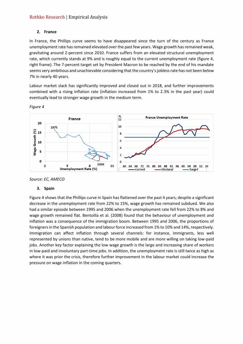
2. France

In France, the Phillips curve seems to have disappeared since the turn of the century as France

unemployment rate has remained elevated over the past few years. Wage growth has remained weak,

gravitating around 2-percent since 2010. France suffers from an elevated structural unemployment

rate, which currently stands at 9% and is roughly equal to the current unemployment rate (figure 4,

right frame). The 7-percent target set by President Macron to be reached by the end of his mandate

seems very ambitious and unachievable considering that the country’s jobless rate has not been below

7% in nearly 40 years.

Labour market slack has significantly improved and closed out in 2018, and further improvements

combined with a rising inflation rate (inflation increased from 1% to 2.3% in the past year) could

eventually lead to stronger wage growth in the medium term.

Figure 4

Source: EC, AMECO

3. Spain

Figure 4 shows that the Phillips curve in Spain has flattened over the past 4 years; despite a significant

decrease in the unemployment rate from 22% to 15%, wage growth has remained subdued. We also

had a similar episode between 1995 and 2006 when the unemployment rate fell from 22% to 8% and

wage growth remained flat. Bentolila et al. (2008) found that the behaviour of unemployment and

inflation was a consequence of the immigration boom. Between 1995 and 2006, the proportions of

foreigners in the Spanish population and labour force increased from 1% to 10% and 14%, respectively.

Immigration can affect inflation through several channels: for instance, immigrants, less well

represented by unions than native, tend to be more mobile and are more willing on taking low-paid

jobs. Another key factor explaining the low wage growth is the large and increasing share of workers

in low-paid and involuntary part-time jobs. In addition, the unemployment rate is still twice as high as

where it was prior the crisis, therefore further improvement in the labour market could increase the

pressure on wage inflation in the coming quarters.

Rothko Research | Empirical Analysis

Figure 5

Source: EC, AMECO

4. Italy

As for Spain and France, the relationship between wage inflation and unemployment flattened in Italy

as well (Figure 6, left frame). The key factors behind the low wage growth are similar to the ones of

Spain: a stagnant productivity and a significant share of workers in low-paid and involuntary part-time

jobs.

Real export performance has significantly lagged euro area peers, and the stagnation of productivity

over the past 10 years has led to a poor change (if any) of the national wellbeing. Figure 6 (right frame)

shows the GDP per capita (real terms) of Italy relative to the two main developed European nations

(Germany and France) since 2000. We observe that in the seven years preceding the Great Financial

Crisis, the three times series had been steadily trending higher with Italy GDP per capital rising from

€29.7K to €31.5K, standing on average between €3,000 and €4,000 below Germany. However, Italy’s

productivity has been non-existent over the past decade, leaving its GDP per capita still at €28.4K in

2017 while the German one was close to €40K (vs. €33.4K in the year 2000).

Figure 6

Source: CEIC, EC, AMECO

Rothko Research | Empirical Analysis

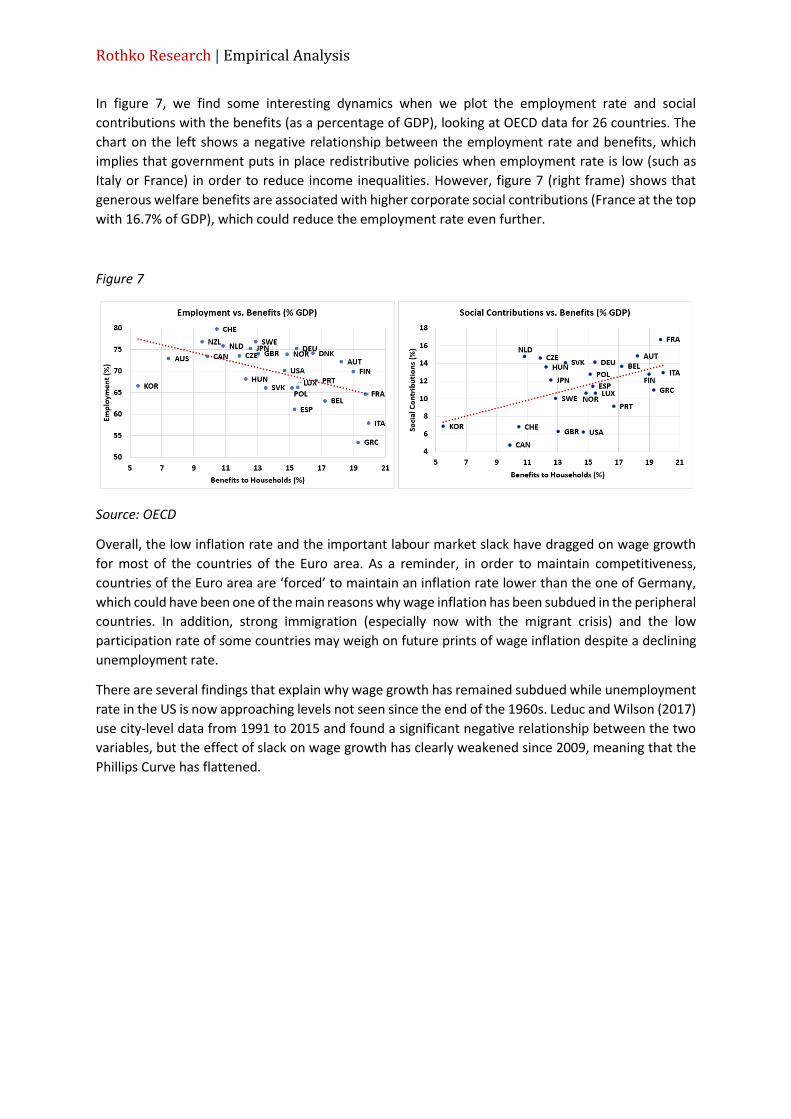
In figure 7, we find some interesting dynamics when we plot the employment rate and social

contributions with the benefits (as a percentage of GDP), looking at OECD data for 26 countries. The

chart on the left shows a negative relationship between the employment rate and benefits, which

implies that government puts in place redistributive policies when employment rate is low (such as

Italy or France) in order to reduce income inequalities. However, figure 7 (right frame) shows that

generous welfare benefits are associated with higher corporate social contributions (France at the top

with 16.7% of GDP), which could reduce the employment rate even further.

Figure 7

Source: OECD

Overall, the low inflation rate and the important labour market slack have dragged on wage growth

for most of the countries of the Euro area. As a reminder, in order to maintain competitiveness,

countries of the Euro area are ‘forced’ to maintain an inflation rate lower than the one of Germany,

which could have been one of the main reasons why wage inflation has been subdued in the peripheral

countries. In addition, strong immigration (especially now with the migrant crisis) and the low

participation rate of some countries may weigh on future prints of wage inflation despite a declining

unemployment rate.

There are several findings that explain why wage growth has remained subdued while unemployment

rate in the US is now approaching levels not seen since the end of the 1960s. Leduc and Wilson (2017)

use city-level data from 1991 to 2015 and found a significant negative relationship between the two

variables, but the effect of slack on wage growth has clearly weakened since 2009, meaning that the

Phillips Curve has flattened.

Rothko Research | Empirical Analysis

II. Wage dynamics

In this part, we review the long-run and short-run determinants of wage growth at the macroeconomic

level. Understanding wage dynamics is a topic that has been approached by many academics and

economists over the past few decades, and especially in the current environment as nominal wage

growth in most advanced countries remains remarkably lower than it was before the Great Financial

Crisis despite tight labour markets.

1. Long Run

According to the economic theory, the long-run determinants of nominal wage growth are the labour

productivity growth and the price inflation. The lower labour productivity reflects weakness in

investment and lower total factor production in the past ten years, and the increase in income and

wealth inequalities may have been driven by the decoupling in wage and productivity growth. Figure

8 shows the sharp decline in productivity growth after the crisis according to a recent report from the

OECD. For instance, in the US and the UK, the labour productivity growth plummeted from roughly 2%

between 2001 and 2007 to roughly 40bps and 25bps, respectively, between 2010 and 2016. Labour

productivity growth remained unchanged in Canada and the Euro Area and was non-existent in Italy

in the period of 2001-2007.

Figure 8

Source: OECD (2018)

We then look at the relationship between the three and try to identify a statistically significant

cointegration. As Abdih and Danninger (2018) did in a recent IMF working paper, we use the

Employment Cost Index (ECI) for compensation of workers in the private sector, the personal

consumption expenditures (PCE) index for price inflation and the real output per hour in nonfarm

business for our labour productivity measure. We then have the following equation:

𝛥𝑤𝑡 = 𝛼 + 𝛽1𝛥𝑝𝑡 + 𝛽2𝛥𝑦𝑡 + 𝜀𝑡

Where 𝛥𝑤𝑡 denotes the nominal wage growth, and 𝛥𝑝𝑡 and 𝛥𝑦𝑡 represent the price and labour

productivity growth rates. We find similar results than Abdih and Danninger (2018), as the coefficient

on inflation (𝛥𝑝𝑡) and labour productivity growth (𝛥𝑦𝑡) have the right signs and are statistically

significant. In their papers, the authors restrict the coefficient on inflation and productivity to -1 (as

they both have negative values) and found that the likelihood ratio tests cannot reject the null

Rothko Research | Empirical Analysis

hypothesis (H0) that both of the coefficients are equal to minus one, and therefore rewrite the model

as the following:

𝛥𝑤𝑡 + 0.9 − 𝛥𝑝𝑡 − 𝛥𝑦𝑡 = 0

Therefore, we have the following relationship:

𝛥𝑤𝑡 = −0.9 + 𝛥𝑝𝑡 + 𝛥𝑦𝑡

Figure 9 represents the residuals of the previous regression (𝛥𝑤𝑡 + 0.9 − 𝛥𝑝𝑡 − 𝛥𝑦𝑡) and we can

notice that times series do mean revert, therefore confirming that the growths do cointegrate into

the stationary linear combination of equation 1.

Figure 9

Source: OECD (2018)

2. Short Run

In the short run, we need to include a slack variable in order to capture cyclical movements in the

wage inflation dynamics. Therefore, our new baseline model is now defined as the following:

𝜋𝑡𝑤 = 𝛼 + 𝛽1 𝑠𝑙𝑎𝑐𝑘𝑡 + 𝛽2 𝑝𝑟𝑜𝑑𝑡 + 𝛽2 𝜋𝑡−2

𝑐 + 𝛽4 𝐸𝑡𝜋𝑡+4 + 𝜀𝑡

Where 𝜋𝑡𝑤 denotes the QoQ nominal wage growth, 𝑔𝑎𝑝𝑡 the level of output gap based on trend real

GDP, 𝑝𝑟𝑜𝑑𝑡 the QoQ changes in labour productivity, 𝜋𝑡−2𝑐 the second lag of changes in core inflation

and 𝐸𝑡𝜋𝑡+4 the 1-year ahead inflation expectations.

a. US

We first run the exercise for the US economy, using the following times series:

- Slack: difference between the current rate of unemployment and the natural rate of

unemployment (NAIRU)

- Prod: labour productivity growth measures as the real output per hour in the non-farm

business sector

-5.4

-5.3

-5.2

-5.1

-5

-4.9

-4.8

-0.15

-0.1

-0.05

0

0.05

0.1

0.15

0.2

0.25

90 92 94 96 98 00 02 04 06 08 10 12 14 16 18

Stationarity vs. Non-stationarity Combinations

Rothko Research | Empirical Analysis

- Core inflation: we use the core CPI measure

- Inflation expectations: we use the University of Michigan’s inflation expectations times series,

which measures the percentage that consumers expect the price of goods and services to

change during the next 12 months

The results of our regression are found in Table 1. To the exception of the coefficient of inflation

expectations, all the other ones are economically and statistically significant. A 1-percent change in

labour productivity (𝑝𝑟𝑜𝑑) is associated with a 0.21% change in wage inflation, and 1-percent change

in core inflation (core) is associated with a 0.54 change in wage inflation. On the other hand, a 1-

percent change in labour slack is associated with a -0.22 change in wage inflation.

Figure 10 shows the positive co-movement between wage inflation and core inflation (left frame) and

the negative co-movement between wage inflation and labour slack (right frame).

Table 1. US wage inflation regression results

Coefficients Standard

Error p-value

Intercept 0.011 *** 0.004 0.00

prod 0.213*** 0.034 0.00

core infl. 0.539*** 0.070 0.00

slack -0.223 0.033 0.00

exp. infl. 0.125 0.104 0.231

R_2 62.9% Obs. 110

*

** ***

10% level 5% level 1% level

Figure 10

Source: FRED, Eikon Reuter

Rothko Research | Empirical Analysis

In figure 11, we first plot the predicted values from our regressors for the entire sample (left frame),

and then we stopped in 2010 to run an out-of-sample analysis (right frame). We can notice that for

the past eight years, our short-run model has been predicting that wages will rise in the US, which has

been the case with the Employment Cost Index up 3.1% in the third quarter of 2018, registering its

highest growth rate in a decade.

Figure 11

Source: FRED, RR, Eikon Reuters

b. UK

As for the US, labour productivity growth plummeted significantly after the financial crisis, declining

from 2% between 2001-2007 to 25bps between 2010-2016 (figure 12, left frame). Using the OECD

data, we also added a scatter plot looking at the change in productivity growth and investment growth

prior and after the crisis (figure 12, right frame). The scale on both axes shows the percentage point

difference between the average growth rates from 1998 to 2007 compared with 2010 to 2016.

Similarly to the US, the UK economy saw a significant 1-percent decline in productivity while the

investment remained unchanged (+0.4%).

Figure 12

Source: ONS, OECD, OBR

Hence, using the same methodology as for the US, we run the regression for the UK wage inflation

dynamics (we used the Bank of England survey for our inflation expectations times series). Results are

reported in Table 2. This time, we can notice that only 2 of our coefficients are significant. Labour

productivity growth has a strong weight in our regression as 1-percent change is associated with a

0.804% change in wage growth. Figure 13 (left frame) shows the strong co-movement between wage

Rothko Research | Empirical Analysis

inflation and labour productivity growth. Surprisingly, the coefficient on core inflation is statistically

significant (at a 5-percent level) but negative, which does not make any economic sense. A 1-percent

increase in core inflation is associated with a 0.573 decrease in wage inflation. Figure 13 (right frame)

shows the negative dynamics between wage growth and core inflation since 1998.

The coefficient on the slack is non-significant in our regression but becomes significant if we use

broader measures of unemployment rates (the p-value of the coefficient is slightly superior to 0.10).

Figure 14 (left frame) shows the inverse relationship between wages and slack. The coefficient on

inflation expectations is also non-significant, however an interesting observation arises when we

overlay the wage growth with inflation expectations (Leading 6M and inverted). It seems that higher

inflation expectations tend to price weaker wage growth (figure 14, right frame).

Table 2. UK wage inflation regression results

Coefficients Standard

Error p-value

Intercept 3.33*** 0.553 0.00

prod 0.804*** 0.122 0.00

core infl. -0.573** 0.221 0.011

slack -0.231 0.146 0.116

exp. infl. -0.045 0.222 0.841

R_2 68.3% Obs. 82

*

** ***

10% level 5% level 1% level

Figure 13

Source: ONS, Eikon Reuters, RR

Rothko Research | Empirical Analysis

Figure 14

Source: ONS, OBR, Eikon Reuters

When we plot our predicted times series, both the in-sample and out-of-sample analyses are showing

weakening signs of wage growth in the UK. This may not apply to all sectors or industries (wages are

rising in construction sector, accommodation and good services or real estate activities); however, it

represents an important challenge for UK policymakers in this period of elevated uncertainty around

the Brexit outcome.

Figure 15

Source: ONS, OBR, Eikon Reuters

c. Euro Area

For the Euro Area, we used the GDP per hour worked as our measure of labour productivity, which is

an annual times series provided by the OECD. We then interpolated the data to transform it to a

quarterly times series. We then use the nominal compensation per employee for our wage inflation

data, which is also an annual times series provided by the European Commission (AMECO database).

As opposed to the US and UK economies, we saw previously that the labour productivity growth has

remained constant in the Euro area prior and after the crisis (Figure 8).

We then run the regression for the Euro area; results are reported in Table 3. Firstly, we can notice

that our measure of labour productivity is non-significant; figure 16 (left frame) shows that there is no

evidence of a strong relationship with wage growth. The coefficient on inflation expectations is also

non-significant, however there seems to be a positive relationship between the two times series in

the long run (figure 16, right frame).

On the other hand, coefficients on core inflation and labour slack are both economically and

statistically significant at a 5-percent and 10-percent level, respectively. A 1-percent in core inflation

leads to a 34bps increase in wage inflation, and a 1-percent increase labour slack leads to a 30bps

contractions wage growth. Figure 17 shows the co-movement between the times series since 1998.

Rothko Research | Empirical Analysis

Table 3. EZ wage inflation regression results

Coefficients Standard

Error p-value

Intercept 0.346 1.605 0.215

prod 0.047 0.063 0.750

core infl. 0.34** 0.143 0.020

slack -0.30* 0.051 0.000

exp. infl. 0.684 0.853 0.425

R_2 56.8% Obs. 82

*

** ***

10% level 5% level 1% level

Figure 16

Source: Eikon Reuters, EC, ECB

Figure 17

Source: Eikon Reuters, EC, ECB

Rothko Research | Empirical Analysis

Our empirical analysis shows that wage growth has been trending higher in the past few years, and

we recently heard ECB President Draghi mentioned that the Governing Council is expecting underlying

inflation to rise in the 19-nation economy as ‘stronger job market pushes up wages’.

Figure 18

Source: Eikon Reuters, EC, RR

To conclude, we saw that the relationship between wages and unemployment has flattened in most

of the advanced economies as a result of a decrease in trade union membership, a rise in self-

employment and rising industrial concertation. As Jonathan Tepper pointed out, as workers have

fewer choices of employer in several industries, industries then have more market power versus their

employees as they become monopolists or oligopolists. However, the relationship is still existent and

the tightness in the labour market globally have been pressuring wage inflation to the upside in the

recent months.

References

Abdih Y. and Danninger S. 2018. Understanding US Wage Dynamics. IMF Working Paper.

Abdih Y., Lin L. and Paret A.-C. 2018. Understanding Euro Area Inflation dynamics. IMF Working Paper.

Bentolila S., Dolado, J. J. and Jimeno J. F. 2008. Does Immigration Affect the Phillips Curve? Some

evidence from Spain. Banco de Espana Working Paper.

Haldane A. 2017. Work, Wages and Monetary Policy. BoE speech.

Leduc, S. and Wilson D. J. 2017. Has the Wage Phillips Curve Gone Dormant? Federal Reserve Bank of

San Francisco.