Phillips Curve and Price‐Change Distribution under .... Phillips Curve and Price‐Change...

Phillips Curve and Price-Change

Distribution under Declining Trend

Inflation

Sohei Kaihatsu * [email protected]

Mitsuru Katagiri ** [email protected]

Noriyuki Shiraki *** [email protected]

No.17-E-5 May 2017

Bank of Japan 2-1-1 Nihonbashi-Hongokucho, Chuo-ku, Tokyo 103-0021, Japan

***Research and Statistics Department, Bank of Japan

***International Monetary Fund

***International Department, Bank of Japan

Papers in the Bank of Japan Working Paper Series are circulated in order to stimulate discussion

and comments. Views expressed are those of authors and do not necessarily reflect those of

the Bank.

If you have any comment or question on the working paper series, please contact each author.

When making a copy or reproduction of the content for commercial purposes, please contact the

Public Relations Department ([email protected]) at the Bank in advance to request

permission. When making a copy or reproduction, the source, Bank of Japan Working Paper

Series, should explicitly be credited.

Bank of Japan Working Paper Series

1

Phillips Curve and Price‐Change Distribution under

Declining Trend Inflation*

Sohei Kaihatsu† Mitsuru Katagiri‡ Noriyuki Shiraki§

May 2017

Abstract

The relationship between the price‐setting behaviors at the micro level and the inflation

dynamics at the macro level is an underexplored research area. In this paper, we first

document that (i) a remarkable shift in cross‐sectional price‐change distributions at the

micro level and (ii) a flattening of Phillips curve at the macro level were simultaneously

observed in Japan, from the high‐inflation periods until the mid‐1990s to the

low‐inflation periods afterward. We, then, empirically show that the menu‐cost

hypothesis fits the price‐setting behavior in Japan and construct a multi‐sector general

equilibrium model with a higher menu cost in the services sector based on our empirical

findings. The quantitative exercise using the model indicates that the above observations

at the micro and macro level in Japan can be consistently replicated within a unified

model under the declining average inflation and the increasing share of services in

output.

JEL classification: E31, E32, E52

Keywords: Phillips curve, Price‐change distribution, Menu cost, Service price rigidity, Deflation,

Trend inflation.

* This research project started when the authors belonged to the Monetary Affairs

Department at the Bank of Japan. We would like to thank the staff of the Bank of Japan for

their helpful comments. We also would like to thank Rie Yamaoka and Yuko Ishibashi for

resourceful research assistance. The opinions expressed here, as well as any remaining errors,

are those of the authors and should not be ascribed to the Bank of Japan or the International

Monetary Fund.

† Research and Statistics Department, Bank of Japan ([email protected])

‡ International Monetary Fund ([email protected])

§ International Department, Bank of Japan ([email protected])

2

1. Introduction

While recent studies using micro data for prices give some insights on price‐setting

behaviors per se, the relation between the price‐setting behaviors at the micro level and

the inflation dynamics at the macro level is still an underexplored and growing research

area.1 In particular, amid rising deflationary pressure in many developed countries,

much attention has been paid to how declining trend inflation affects price‐setting

behaviors at the micro level, and how the changes in price‐setting behaviors, in turn,

affect the inflation dynamics at the macro level.

To understand the relation between the micro and macro price dynamics under the

declining trend inflation, the Japanese experience from the high‐inflation periods (1982–

1994 FY) to the low‐inflation periods (1995–2012 FY) gives the following

thought‐provoking stylized‐facts. First, at the micro level, a remarkable shift in

cross‐sectional price‐change distributions has been observed. Specifically, along with the

decline in average inflation, the price‐change distributions in the services sector have

been weighted more heavily around 0% and its dispersion has narrowed, while the

distributions in the goods sector only shifted leftward. Second, at the macro level, the

Phillips curve—the relation between inflation and macroeconomic demand‐supply

balance—has flattened in both goods and services sectors. That is, as average inflation

has declined, price sensitivity to business cycles has also declined in both sectors. In

contrast to the sectoral differences in the micro‐level price‐setting behaviors, the

flattening of the Phillips curve has been observed not only in the services sector but also

in the goods sector.

The purpose of this paper is to provide a consistent explanation for the stylized‐facts

observed at the micro and macro levels in Japan and deepen our understanding of the

relationship between firms’ price‐setting behaviors and their macroeconomic

consequences. Specifically, we show that the menu‐cost hypothesis can explain both the

flattening of the Phillips curve and the shifts in the price‐change distributions in a

1 As empirical studies using micro data for prices, see Bils and Klenow (2004), Klenow and

Kryvtsov (2008), Nakamura and Steinsson (2008, 2013) for the U.S., Higo and Saita (2007),

Kurachi et al. (2016) for Japan, and Dhyne et al. (2006) for the Euro area.

3

consistent way. To consider the validity of the menu‐cost hypothesis, we carry out both

empirical and theoretical studies.

In the empirical part, we set up an empirical model with price rigidities in the

vicinity of a 0% inflation rate to test the menu‐cost hypothesis. Specifically, we employ a

panel data analysis using a limited dependent variable model with two‐sided thresholds,

which is used by the recent study of Honoré et al. (2012). Employing the empirical model,

we estimate parameters regarding the menu‐cost hypothesis based on individual item

data of Consumer Price Index (CPI). In order to adequately identify menu‐cost

parameters, we extract common factors such as demand and supply shocks from the

large macroeconomic dataset using a principal component approach as in Boivin et al.

(2009). We then use these factors as explanatory variables to control for macroeconomic

factors driving price fluctuations. Our empirical study indicates higher menu cost in the

services sector than in the goods sector, which is consistent with our empirical findings

regarding price‐change distributions and other empirical studies such as Nakamura and

Steinsson (2010) for U.S. or Dhyne et al. (2006) for the Euro area.

In the theoretical part, we examine whether the menu‐cost hypothesis can

consistently explain the observed shift in price‐change distributions by sector as well as

the flattening of the Phillips curve under shifting trend inflation within a unified model.

For this purpose, we construct a multisector dynamic general equilibrium model with

heterogeneous firms and assume that the services sector bears higher menu cost than the

goods sector, following our findings in the empirical part. We then calibrate the model

parameters to replicate some moments regarding the observed cross‐sectional

distributions of price changes in both goods and services sectors. Using the calibrated

model, we explore how shifts in trend inflation as well as the share of services in total

output affect the slope of the Phillips curve through changes in price‐change

distributions. Our quantitative results of the comparative statics with respect to the shift

in trend inflation as well as the share of services in total output lead to the following two

findings. First, the multisector menu‐cost model can adequately replicate the change in

price‐change distributions in both goods and services sectors. Second, the model can

also replicate almost the same degree of flattening of the Phillips curves as observed

during the deflationary period in Japan in both sectors. These findings imply that the

4

menu‐cost hypothesis can consistently account for the change in firms’ price‐setting

behaviors during the deflationary period in Japan and its macroeconomic consequences.

The relationship between the Phillips curve and the menu cost is a classical topic

discussed by, for example, Ball et al. (1988). They imply that, based on the menu‐cost

hypothesis, a decline in trend inflation rates increases price rigidities and makes the

Phillips curve flatter.2 Recently, a number of studies have shed new light on this topic on

the basis of a general equilibrium model with a menu‐cost element (e.g., Golosov and

Lucas, 2007; Midrigan, 2011; Vavra, 2014; Kehoe and Midrigan, 2015; Watanabe and

Watanabe, 2017). In particular, the most closely related studies to the current paper are

Enomoto (2007) and Nakamura and Steinsson (2010), which examine a price‐setting

behavior and monetary neutrality using a multisector general equilibrium model with a

menu cost.3 The current paper belongs to this line of research, by assessing whether a

multi‐sector general equilibrium model with a menu cost adequately explains the

observed shift in price‐change distributions by sector as well as the flattening of the

Phillips curve, both of which were observed during the deflationary period in Japan.

The remainder of the paper proceeds as follow. Section 2 shows empirical findings

about shifting price‐change distributions and the changing slope of the Phillips curve

during the deflationary period in Japan. Section 3 describes the menu‐cost hypothesis

and an empirical procedure to test the plausibility of the menu‐cost hypothesis. In

Section 4, we construct a multisector general equilibrium model with the heterogeneous

menu‐cost structure across sectors. Section 5 shows quantitative analyses based on the

theoretical model. Section 6 presents the conclusion.

2 Following Ball et al. (1988), there is another line of research investigating time‐varying price

stickiness by endogenizing the degree of nominal rigidities in a Calvo‐style sticky price

models (see Romer, 1990; Kiley, 2000; Devereux and Yetman, 2002; Levin and Yun, 2007;

Kimura and Kurozumi, 2010; Kurozumi, 2016).

3 In terms of methodology and motivation, while those two papers use a classic monetary

model with money supply shocks and focus on monetary neutrality, the current paper uses a

model with an interest rate feedback rule by central banks and focus on business cycles

driven by demand shocks in line with the recent quantitative monetary economics literature.

5

2. Price‐Change Distributions and the Phillips Curve

In this section, we first describe the micro‐level price dataset we use in this paper and

explain the filtering method which we apply to the price data. We then examine

price‐change distributions, the frequency of price adjustments, and the slope of the

Phillips curve during the period of declining average inflation in Japan since the late

1980s.

2.1 Price‐Change Distribution

Our dataset covers the 588 price indices of individual items composing the CPI.4 Before

analyses, we removed temporary price changes from each price series. Recent works

such as Bils and Klenow (2004) show that micro‐level price series fluctuate much more

frequently than the aggregate ones. To give consistent explanations for price‐setting

behaviors at both the macro and micro levels, Kehoe and Midrigan (2015) emphasize the

need to distinguish temporary and regular price changes in the micro‐level price series.

They also show that temporary price changes in the micro‐level price data do not affect

the aggregate price rigidity, based on the theoretical analysis.

Therefore, to derive implications for the aggregate price rigidity from the micro‐level

price‐change distributions, we need to remove temporary price changes from the

original price series. We adopt a simplified method developed by Kehoe and Midrigan

(2015) to remove temporary price changes. Specifically, the five‐month centered running

mode of the original price series is computed.5 This type of algorithm is employed by,

for example, Eichenbaum et al. (2011) and Sudo et al. (2014).

After the above filtering, we examine developments of price‐change distributions

during both the inflationary and deflationary periods in Japan. First, we examine the

4 Recently, there are some studies using scanner data for investigating micro price dynamics

in Japan (see Abe and Tonogi, 2010; Sudo et al., 2014). However, they focus only on goods

prices because the most of the scanner data includes few service prices. In this paper, we use

CPI individual data including 141 individual service prices for investigating both goods and

services price dynamics.

5 We define the most frequent price over five months as the regular price and identify the

difference between the actual and regular prices as the temporary price change.

6

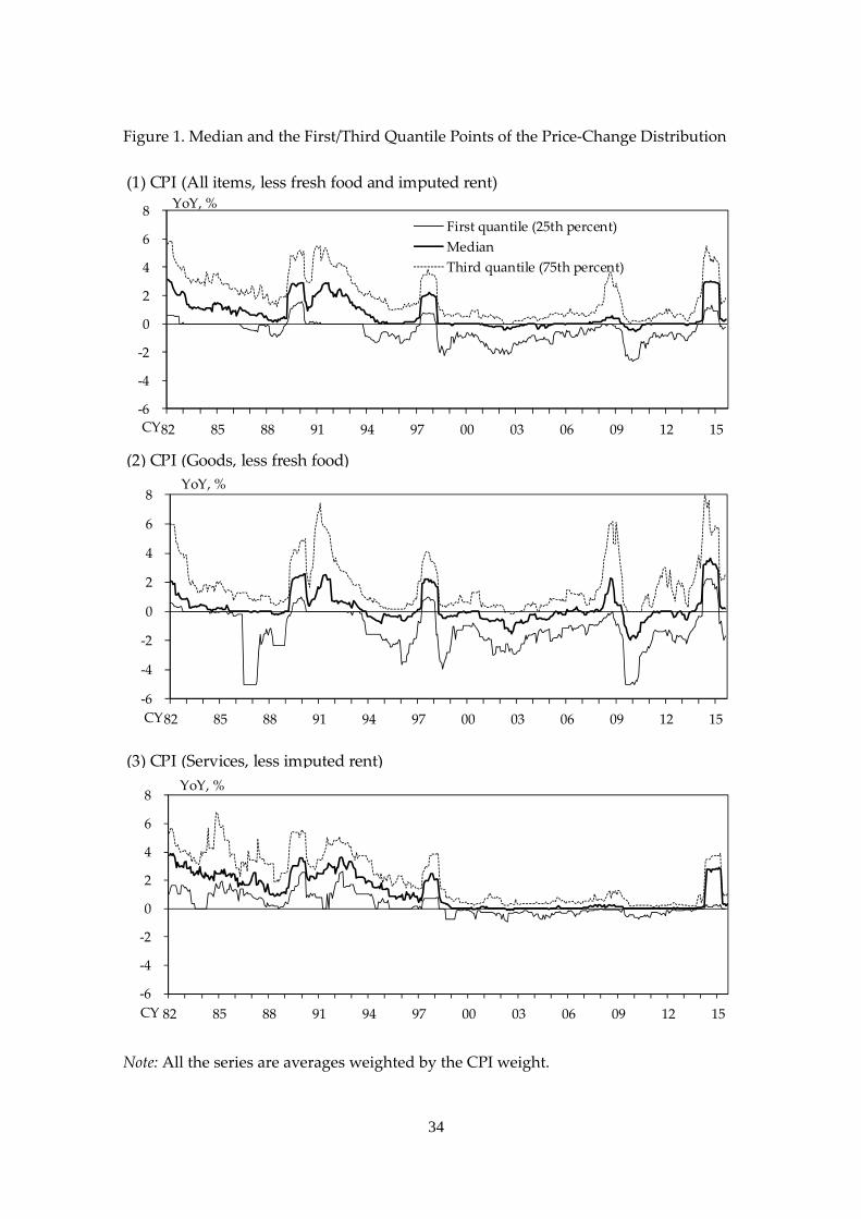
dispersion of distributions by focusing on weighted quantile points.6 Figure 1 shows

developments of first/second (i.e., median)/third weighted quantile points from a

high‐inflation period (1982–1994 FY) to a low‐inflation period (1995–2012 FY) by sector.

According to Figure 1 (1) for CPI (all items, less fresh food and imputed rent), the

weighted median remained in the vicinity of 0% and the range from first to third

quantiles became narrower from the high to low‐inflation period.7 However, there is

large heterogeneity across goods and services. For goods prices, Figure 1 (2) shows that

each quantile point moved smoothly and the range from first to third quantiles was

approximately constant in both the high‐ and low‐inflation periods. Meanwhile, Figure 1

(3) for service prices shows that the range from first to third quantiles became quite

narrower during the same period and the weighted median remained in the vicinity of

0%. These facts imply that from the high to low‐inflation period, price rigidity

dramatically increased in the services sector, whereas it was nearly stable in the goods

sector.

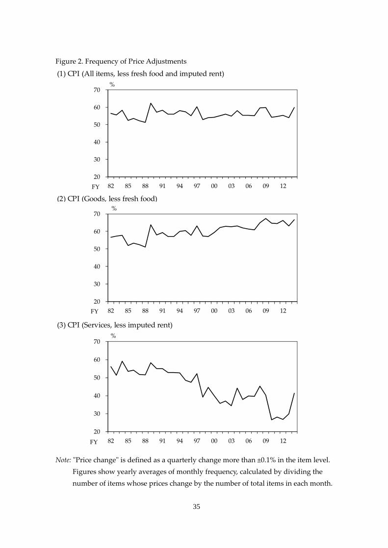
The increase of price rigidity in the services sector can be also confirmed by the

frequency of price adjustments. Figure 2 provides the frequency of price adjustments.8

While the frequency of price adjustments had increased moderately for goods, it had

significantly decreased since the late 1990s for services.9 This implies that only service

price rigidity had increased along with the decline in average inflation.

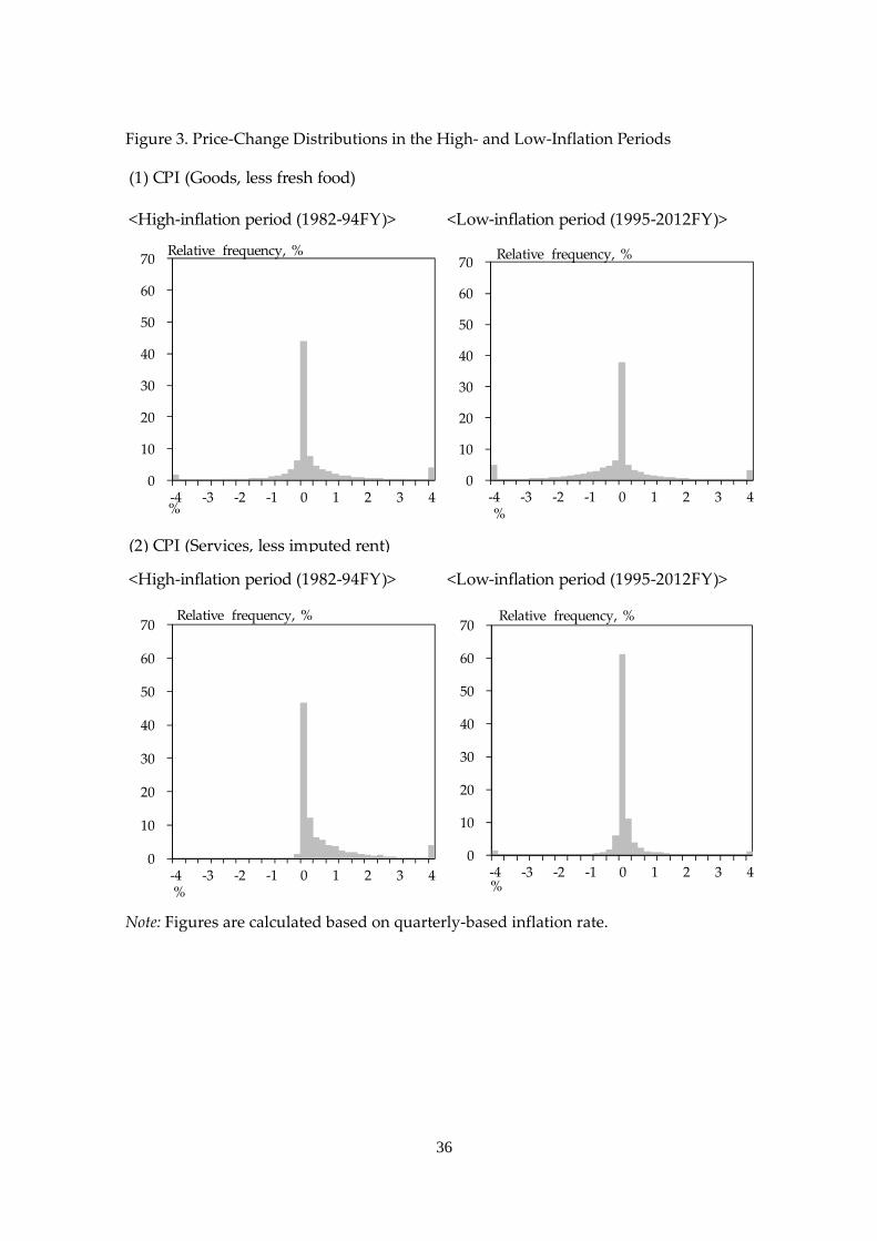
Finally, Figure 3 displays price‐change distributions in the high‐ and low‐inflation

period. In the goods sector, the price‐change distribution only shifted leftward, with the

weight in the vicinity of 0% almost unchanged. In the services sector, however, the shape

of distribution changed dramatically from the high to the low‐inflation period; (i) the

6 Weighted quantile is calculated from weighted distribution based on the CPI weight (2010

year basis) of each individual item. As a robustness check, we confirm that our main results

do not change with alternative weights in the years 2000 and 2005.

7 We exclude the price of imputed rent from the data because it does not reflect

macroeconomic demand‐supply balance directly. As a robustness check, we confirm that our

main results do not change with the data including imputed rent.

8 “Price change” is defined as a quarterly change more than ±0.1% in the item level.

9 This observation is consistent with Higo and Saita (2007) and Kurachi et al. (2016).

7

distribution had more weight in the vicinity of 0%, (ii) the dispersion became narrower,

and (iii) the positive skewness observed in the high inflation period disappeared.

2.2 Phillips Curves

In this section, we examine changes in the slope of the Phillips curve. The slope of the

Phillips curve indicates the degree of output‐inflation tradeoff. In other words, it is a

parameter that links nominal and real economic activities. In that sense, identifying the

slope of the Phillips curve is important for central banks to achieve their price stability

target.

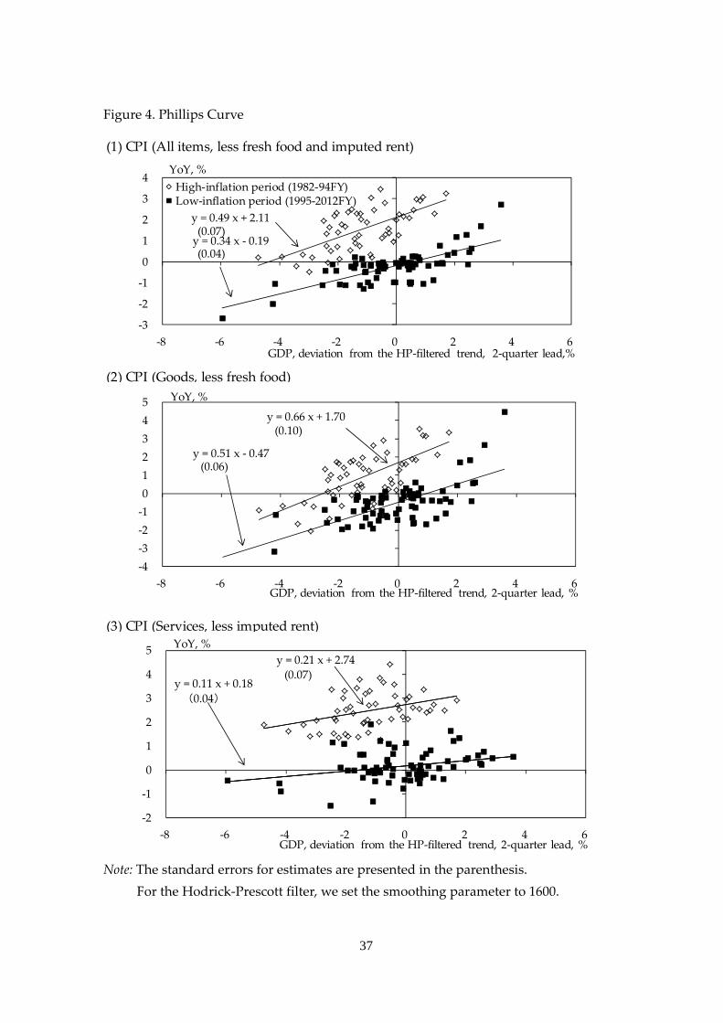
Many previous studies investigating the Phillips curve in Japan provide evidence for

flattening of the Phillips curve during the deflationary period. For example, De Veirman

(2009) and Kaihatsu and Nakajima (2015) estimate the slope of the Phillips curve and

report that the Phillips curve had flattened in the 1990s. Figure 4 displays the slope of

the Phillips curve for CPI inflation rate (all items, goods, and services) in both the high‐

and low‐inflation periods.10 We find that the Phillips curve had significantly flattened

from the high‐inflation periods to the low‐inflation periods in both goods and services

sectors.

2.3 Implications of the Menu‐Cost Hypothesis

The observed shift in price‐change distributions and the changing slope of the Phillips

curve are potentially explained by the menu‐cost hypothesis in a consistent manner.

With the menu cost, firms must pay fixed costs in order to change their prices. If trend

inflation declines in this situation, firms’ incentive to change prices decreases because

relative prices change only moderately. Consequently, the frequency of price

adjustments decreases and the price‐change distribution is likely to have more weight in

the vicinity of 0% and narrower dispersion. From the macroeconomic point of view, the

Phillips curve becomes flatter because a decreased frequency of price adjustments

reduces the sensitivity to shocks from the real economy (Ball et al., 1988).

10 Note that the degree of flattening of Phillips curve depends on the data used for

estimation.

8

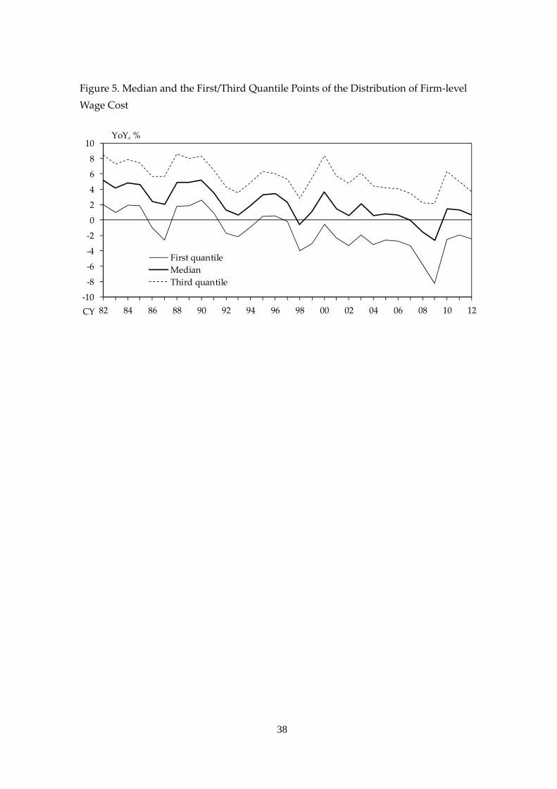
There may be another explanation for the observed shift in price‐change distributions

and the changing slope of the Phillips curve during a deflationary period: the downward

nominal rigidity of wages (see Akerlof et al., 1996). We do not deny the influence of

downward wage rigidity, since it does not necessarily contradict the menu‐cost

hypothesis. However, it would not be empirically supported that the increasing price

rigidity during the deflationary period is accounted for only by downward nominal

rigidity in wages. Figure 5 shows the development of quantile points in a firm‐level

wage cost distribution per head. The figure indicates that quantile points move smoothly

even in the deflationary period in Japan after mid‐1990s, which implies that workers

started to accept nominal wage cuts in Japan (see also Kuroda and Yamamoto, 2003).11

Another issue is how we can reconcile the flattening Phillips curve in goods sector

with the micro evidence that goods‐price rigidity has been almost unchanged. There are

several consistent explanations for this issue. For example, increasing competitiveness

by deregulation or globalization (see Gaiotti, 2010), or strengthening commitment for

anchoring inflation expectations by monetary authorities (see Boivin et al., 2010), could

make the Phillips curve flatter. In particular, globalization could affect the goods sector

more strongly than the services sector because goods are tradable. Another possible

explanation is the influence of interaction between the goods and services sectors via

general equilibrium effects. In this regard, increasing price rigidity in the services sector

could somehow affect the goods‐price rigidity. We will take up this point later by

constructing the general equilibrium model.

3. Empirical Analysis of the Menu‐Cost Model

In this section, to assess the validity of the menu‐cost hypothesis, we estimate a limited

dependent variable model with two‐sided thresholds, following Sekine and Tachibana

(2004) and Honoré et al. (2012).

11 Although some downward rigidity was observed in regular wages, Japanese firms flexibly

adjusted nominal wages by changing bonuses, comprising a large fraction of total wages in

Japan.

9

3.1 Empirical Specification

Our empirical model is closely related to that in Honoré et al. (2012), which specifies a

reduced form of the menu‐cost model; firms would change their prices only if the

optimal level of inflation rate (the latent inflation rate, hereafter) is significantly different

from zero. Here, the latent inflation rate is an unobservable variable, which is supposed

to reflect exogenous conditions, including various factors such as demand and supply

shocks. The threshold for firms beyond which they change their prices is determined by

the menu cost that firms must pay for changing their prices.

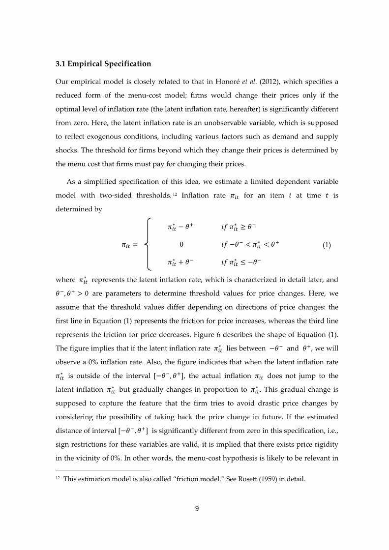
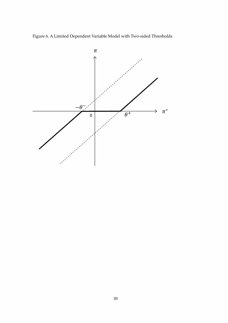
As a simplified specification of this idea, we estimate a limited dependent variable

model with two‐sided thresholds. 12 Inflation rate for an item at time is

determined by

∗ ∗

(1) 0 ∗

∗ ∗

where ∗ represents the latent inflation rate, which is characterized in detail later, and

, 0 are parameters to determine threshold values for price changes. Here, we

assume that the threshold values differ depending on directions of price changes: the

first line in Equation (1) represents the friction for price increases, whereas the third line

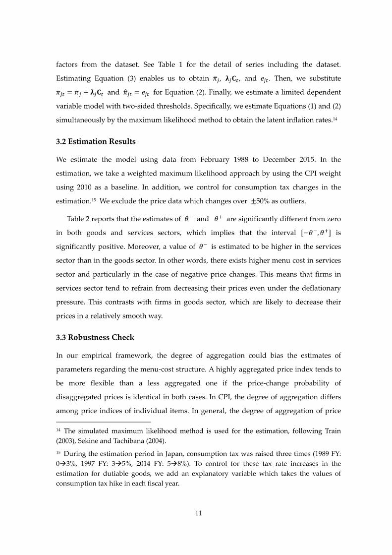
represents the friction for price decreases. Figure 6 describes the shape of Equation (1).

The figure implies that if the latent inflation rate ∗ lies between and , we will

observe a 0% inflation rate. Also, the figure indicates that when the latent inflation rate

∗ is outside of the interval [ , , the actual inflation does not jump to the

latent inflation ∗ but gradually changes in proportion to ∗ . This gradual change is

supposed to capture the feature that the firm tries to avoid drastic price changes by

considering the possibility of taking back the price change in future. If the estimated

distance of interval [ , is significantly different from zero in this specification, i.e.,

sign restrictions for these variables are valid, it is implied that there exists price rigidity

in the vicinity of 0%. In other words, the menu‐cost hypothesis is likely to be relevant in

12 This estimation model is also called “friction model.” See Rosett (1959) in detail.

firms

T

rate,

deter

we s

Hono

main

laten

secto

et al.

wher

that

IIN(0

class

non‐

T

the f

vecto

corre

rate

each

To id

comp

prod

13 Bo

perce

s’ price‐setti

The issue in

∗ . This i

rmined to r

specify this

oré et al. (2

nly driven b

nt inflation r

oral inflation

(2012), the

re deno

an individu

0, ) proce

sification pr

durable goo

To specify s

following m

or of com

esponding f

can be

sector

dentify the

ponent app

duction, and

oivin et al.

ent of month

ing behavio

n empirical

is because

reflect vario

s unobserva

2012). These

by sectoral i

rate. Specifi

n trend and

empirical s

otes sectora

ual item i b

ess. Each se

rovided by

ods, public

sectoral infl

model. Let

mon macr

factor loadi

decompose

, and an id

e vector of

proach. We

d consumpt

(2010) show

hly fluctuati

ors.

estimation

the latent i

ous factors s

able variabl

e studies sh

inflations; h

ically, we as

d sector‐spe

pecification

∗

al inflation t

belongs to,

ector is clas

y the Statis

services, an

ation trend

denote

oeconomic

ings for ea

ed into a sec

diosyncratic

f common

construct la

tion of good

wed that th

ons in disag

10

of the mod

inflation ra

such as dem

le based on

how that pr

hence, we u

ssume that t

ecific deviat

n reads

trend, d

, and d

ssified as on

stic Bureau

nd private s

d and s

the actual

shocks, a

ach variable

ctoral inflat

componen

macroecon

arge macroe

ds or service

he sector‐spe

ggregated pr

del is how t

ate is the u

mand and s

n the ideas

rice fluctuat

se them as

the latent in

tions from it

,

denotes sec

enotes an i

ne of the fol

u: durable

services.

sector‐specif

inflation ra

and den

e. We assum

tion average

nt ( ):

nomic shoc

economic d

es and extra

ecific shock

rices.

to specify th

unobservabl

supply shoc

s of Boivin

tions of ind

a proxy for

nflation rate

ts trend.13 F

tor‐specific

idiosyncrati

llowing five

goods, sem

fic shocks

ate in secto

notes the

me that eac

e , comm

cks , we

dataset inclu

act four prin

ks account o

he latent in

le variable

cks. In this

n et al. (201

dividual ite

r the change

e depends o

Following H

shocks in s

ic error fol

e sectors ba

mi‐durable

, we est

or , den

estimates

ch actual in

mon compon

e use a pr

uding input

ncipal comp

on average

nflation

that is

paper,

0) and

ms are

e in the

on both

Honoré

(2)

sector

lowing

ased on

goods,

imated

notes a

of the

nflation

nent on

(3)

rincipal

t price,

ponent

for 85

11

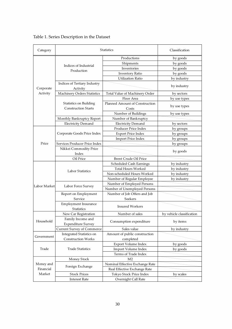
factors from the dataset. See Table 1 for the detail of series including the dataset.

Estimating Equation (3) enables us to obtain , , and . Then, we substitute

and for Equation (2). Finally, we estimate a limited dependent

variable model with two‐sided thresholds. Specifically, we estimate Equations (1) and (2)

simultaneously by the maximum likelihood method to obtain the latent inflation rates.14

3.2 Estimation Results

We estimate the model using data from February 1988 to December 2015. In the

estimation, we take a weighted maximum likelihood approach by using the CPI weight

using 2010 as a baseline. In addition, we control for consumption tax changes in the

estimation.15 We exclude the price data which changes over 50% as outliers.

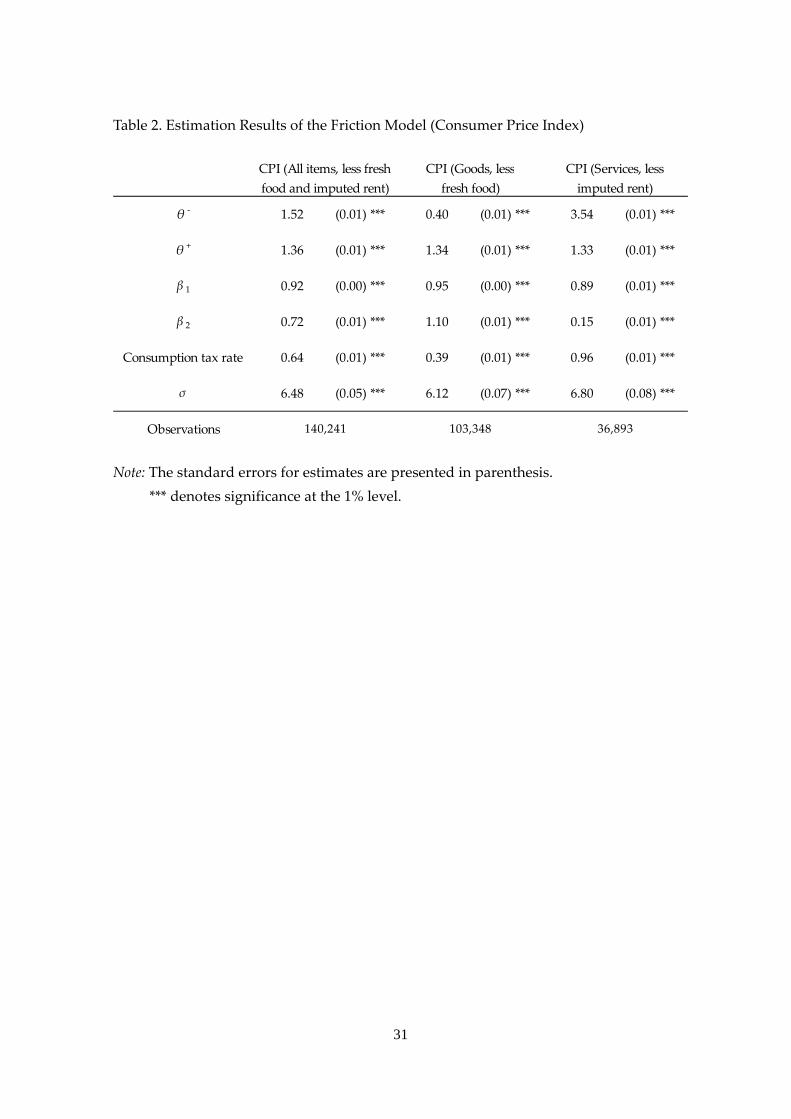
Table 2 reports that the estimates of and are significantly different from zero

in both goods and services sectors, which implies that the interval , is

significantly positive. Moreover, a value of is estimated to be higher in the services

sector than in the goods sector. In other words, there exists higher menu cost in services

sector and particularly in the case of negative price changes. This means that firms in

services sector tend to refrain from decreasing their prices even under the deflationary

pressure. This contrasts with firms in goods sector, which are likely to decrease their

prices in a relatively smooth way.

3.3 Robustness Check

In our empirical framework, the degree of aggregation could bias the estimates of

parameters regarding the menu‐cost structure. A highly aggregated price index tends to

be more flexible than a less aggregated one if the price‐change probability of

disaggregated prices is identical in both cases. In CPI, the degree of aggregation differs

among price indices of individual items. In general, the degree of aggregation of price

14 The simulated maximum likelihood method is used for the estimation, following Train

(2003), Sekine and Tachibana (2004).

15 During the estimation period in Japan, consumption tax was raised three times (1989 FY:

03%, 1997 FY: 35%, 2014 FY: 58%). To control for these tax rate increases in the

estimation for dutiable goods, we add an explanatory variable which takes the values of

consumption tax hike in each fiscal year.

12

indices in the services sector tends to be lower than that in the goods sector because the

number of samples in the services sector is generally smaller than that in the goods

sector due to difficulty in data collection. Therefore, the result of the previous section

that the services sector bears a higher menu cost than the goods sector could be biased

by the lower degree of aggregation in the services sector.

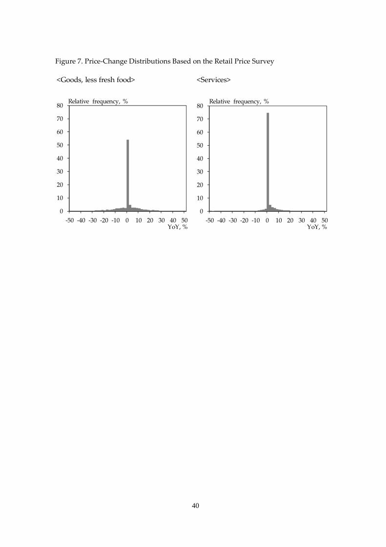
As a robustness check, we carry out the same estimation procedure for the Retail

Price Survey (RPS) instead of the CPI data. RPS, which is conducted by the Statistics

Bureau, is used as basic data for calculating CPI. In this sense, RPS is more

disaggregated price data than CPI, although a certain number of items, such as a car and

a mobile phone, are not covered by RPS. Furthermore, it is worth noting that RPS is not

perfectly disaggregated data; the price series of RPS is released as an average of prices

collected in each city. The number of collected prices is different among cities and ranges

from 1 to 42 according to city size. To avoid the influence of aggregation issues, we

restrict our dataset to RPS data series that consist of only 1 price data.

Figure 7 displays the price‐change distribution based on RPS. In goods and services

sectors, the proportion of 0% inflation is higher in RPS than in CPI (Figure 3). This

implies that the aggregation process might affect the observed price rigidity in both

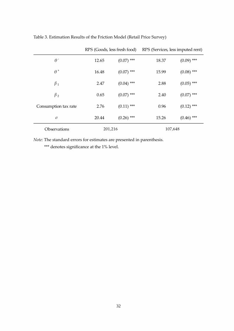
sectors. In Table 3, however, the estimation result shows that the distance of interval

, is significantly positive in both sectors, implying that price rigidities in the

vicinity of 0% exist. In addition, the estimate is higher in the services sector than in

the goods sector. These results are consistent with those obtained by the estimation

based on the CPI data, as shown in the previous subsection. On the whole, this

robustness check confirms the menu‐cost hypothesis based on more disaggregated price

data. Furthermore, both and are higher than those based on the CPI data. This

result implies that the data aggregation tend to make it difficult to observe price rigidity,

compared with the case of disaggregated price data.

4. Multisector Menu‐Cost Model

In this section, we investigate the macroeconomic implications of each firmʹs

price‐setting behavior by constructing a multisector menu‐cost model. In particular, we

13

focus on the relationship of flattening of the Phillips curve with a decline in trend

inflation and with a rise in the share of services in Japan. We examine whether such a

relationship can be explained consistently with the microeconomic price‐setting

behavior described in the previous sections.

The model in this section is a multisector version of a general equilibrium menu‐cost

model with heterogeneous firms, such as the one given in Midrigan (2011). One sector

with a lower menu cost corresponds to a goods sector, while the other sector with higher

menu cost corresponds to the services sector.

The private sector of the economy consists of a representative household,

consumption‐good firms, and intermediate‐good firms. The intermediate‐good firms in

each sector are heterogeneous with respect to their productivity and maximize their

profits by choosing their prices under both a state‐dependent and time‐dependent

nominal friction. The central bank conducts monetary policy using the nominal interest

rate as a policy tool. Each agentʹs behavior is described in turn.

4.1 Household

The representative household supplies a labor force to obtain wage income, , where

denotes the nominal wage and denotes hours worked. In addition, because the

household owns all firms in the economy as a stockholder, it also obtains a nominal

dividend, , as another source of income. The household allocates its income to a

consumption basket, , and savings as a form of nominal one‐period bond, . The

household faces the budget constraint

(4)

where is the price level and is the gross nominal interest rate. The consumption

basket consists of goods, denoted by , and services, denoted by , with the weight ,

, 1 , ,

where is a parameter for elasticity between goods and services. The price level of the

consumption basket is defined by , , , , as usual. Given those

14

conditions, the household maximizes its expected lifetime utility by choosing

consumption and labor supplies

max, , , , ,

log ,

subject to the budget constraint (4). ∈ 0,1 is a constant discount factor, is a shock

to the discount factor, and is the disutility of labor.

The optimal allocation between goods and services gives the price indicator

, 1 , , (5)

as well as the demand function for consumption in each sector

, , and , , , (6)

where , ≡ , is a relative price in sector ∈ , . Also, the first order

conditions for , , and give the Euler equation

1 , (7)

where and , as well as the labor supply function

, (8)

where is a real wage rate. Finally, the stochastic discount factor is defined

as

, , ≡ . (9)

As is shown later, firms maximize the sequence of profits discounted by this stochastic

discount factor.

4.2 Central Bank

The central bank sets the nominal interest rate according to a type of Taylor rule

responding only to inflation rates,

∗ , (10)

15

where ∗ is the target inflation rate, which is identical to trend inflation in steady state,

and ∗ is the nominal interest rate at the steady state. We assume 1 so

that the Taylor principle holds.

4.3 Firm

The consumption‐good firm in sector ∈ , produces the final good, , , using the

intermediate goods, , , , produced by firm in sector using the following CES

aggregator, , , , , where 1 is the elasticity of substitution. Let

, , be the price of each intermediate good. The price index, , , is then defined as

, , , , (11)

and the demand for each intermediate good is derived as a result of profit maximization

of the representative consumption‐good firm,

, , , , , , (12)

where , , ≡ , , , is a relative price of the differentiated goods produced by firm

.

A continuum of intermediate‐good firms produces differentiated intermediate goods

using labor, , , , according to the following linear technology,

, , , , , , , (13)

where , , is an idiosyncratic productivity for firm in sector at period . The

profit for firm in sector before subtracting the menu cost, , , , , , ; , , is

, , , , , ; ,, ,

,, , , ,

(14)

, ,, ,

, , , .

The last equation comes from (8), (12), (13), and the market clearing condition .

Under monopolistic competition, the intermediate‐good firm in sector sets the price

of its differentiated products and maximizes the sequence of profits, , , , , , ; , ,

discounted by the stochastic discount factor, , , , subject to the sequence

of aggregate state variables, , , , , , , , , , , and .

16

4.4 Characterization of Equilibrium

First, the stochastic processes for structural shocks are specified. In this model, we

assume one aggregate shock, , and one idiosyncratic shock, , . The growth rate of

discount rate shock is assumed to follow the AR(1) process,

log log , , (15)

where , follows 0, . The idiosyncratic productivity shock for firm in sector

is also assumed to follow the AR(1) process, but the shock to the idiosyncratic

productivity arrives only with probability ,

, ,

, , exp, , with prob.

(16)

, , with prob. 1 ,

where , , follows 0, , . The assumption of infrequent shocks is incorporated to

account for the fat‐tailed distribution of price changes observed in data.16 Note also that

the volatility of idiosyncratic productivity shocks , could be different in each sector.

In a quantitative analysis, we discretize the state space for , , and , and

approximate the AR(1) process by a first order Markov process with different value of

volatility by sector.

In order to solve the model, we need to calculate aggregate state variables by

aggregating each firm‐specific variable. Computing aggregate state variables is, however,

not trivial in this model because of heterogeneity in firmʹs productivity. Therefore, we

make some assumptions to make the model computationally tractable. First, we assume

that the elasticity between goods and services is equal to that between intermediate

goods in each sector, i.e., . Under this assumption, the demand functions (6) and

(12) imply

, , , , (17)

16 While this assumption improves the model fit, it does not affect main results in this paper

including the skewness of price change distribution.

17

where , ≡ , , . Since the demand for intermediate‐good firm is now a function

of the aggregate demand and the relative price to the aggregate price, and , , the

demand and the relative price in each sector, , and , , are not relevant for each

firmʹs optimization and consequently can be dropped from the aggregate state variables.

Second, according to Krusell and Smith (1998) and its application to a menu‐cost model

such as Midrigan (2011) and Vavra (2014), the law of motion for a key macroeconomic

state variable is approximated by a linear function. In particular, we assume that the

aggregate demand follows the AR(1) process with variable constant terms with respect

to and after log‐transformation,

log , , log , (18)

where , , , , and are constant terms (i.e., fixed effects) corresponding to each

grid of and .

Given the law of motion for approximated by (18), the inflation rate can be

expressed as a function of and . By plugging nominal interest rates by the Taylor

rule (10) into the Euler equation (7), we have the following forward equation for

inflation,

∗ ⋯ .

Since we assume that follows the AR(1) process and that is a function of

, , and as described in (18), the right hand side of the equation can be

computed one by one. Furthermore, as long as 1, each term in the right hand side

converges to zero. In a quantitative analysis, we stop the calculation at twenty terms,

∗ , (19)

because the value of inflation does not change significantly even if the number of terms

for calculation is increased to more than twenty.

When the intermediate‐good firm chooses its relative prices, , , it is faced with the

following state‐dependent and time‐dependent nominal frictions. First, the firm obtains

the opportunity for price changes with probability ∈ 0, 1 in every period, exactly as

18

in the Calvo model. Second, upon obtaining the opportunity for price changes, the firm

faces the menu cost with probability ∈ 0, 1 . Therefore, while the firm faces zero

menu cost and must change its prices with probability 1 , the firm faces a positive

menu cost and solves the discrete choice problem between changing its prices and not

changing them with probability . This assumption of zero menu cost with a small

probability is incorporated to account for the small price changes observed in data and is

used in other studies including Vavra (2014). In the discrete choice problem for price

setting, we assume that each firm stochastically makes their decisions. That is, the

fraction of firms who change prices is denoted by ∙ ∈ 0, 1 and expressed as a

function of state variables as in a generalized Ss‐model in Caballero and Engel (2007).

Finally, each firmʹs optimization problem is characterized recursively. The value

function for the intermediate‐good firm in sector , which is denoted by

, , ; , , has two individual state variables, and , , as well as two aggregate

state variables, and , and consists of three value functions. Given the constraints (9),

(14), (15), (16), (18), and (19), the optimization problem for each intermediate‐good firm

in sector is formulated by the value function,

, , ; , , ,,

, , ; , 1 , ; ,

1 , , ; ,

where , , and are the value function for the discrete choice problem, the value

function for changing prices and the value function for not changing prices, respectively.

Also, ⋅,⋅,⋅ is a stochastic discount factor defined in (9). The value function for the

discrete choice problem, , , ; , , is formulated as

, , ; , , , ; , , ; ,

1 , , ; , , , ; , .

Note that the firms have to pay the menu cost when they change prices and obtain

. The fraction of firms who change prices, , , ; , , is defined as

, , ; , , ; , , , ; , , , , , ,

19

where ∙, , , , is a cumulative distribution function of a Gamma distribution with

parameter , and , . Since ∙, , , , is an increasing function in 0, 1 , the above

definition of ∙ implies that the fraction of firms who change prices approaches one

(zero) as the net benefit of changing prices increases (decreases). Finally, the value

function for changing prices, , ; , , and that for not changing

prices, , , ; , , are formulated as

, ; , max , , ; , , ; , ,

and

, , ; , , , ; , , ; , .

Those two value functions show that when the firm changes prices, it can choose an

optimal level of relative price , and the current profit and future value are computed

based on the optimal . When the firm does not change prices, the relative price for

the firmʹs products is deflated by inflation rate , and the current profit and

future value are evaluated based on the deflated relative price, . By solving the

optimization problem for each sector , we have the following two policy functions: the

optimal choice of relative prices if the firm changes the price, ∗ , , ; , and the

optimal probability to change the price, ∗ , , ; , .

The procedure to compute a recursive competitive equilibrium is as follows. First,

given an initial guess for the coefficients , , , , and in the conjectured law of

motion (18), we solve the optimization problem for firm , which is recursively

formulated by value functions. Once the optimal policy function for price setting is

obtained, we construct a simulated path of aggregate demand under the artificially

generated sequence of and the optimal policy function of . In order to construct

the simulated path of aggregate demand, we search for that satisfies the consistency

of aggregate price (i.e., the market clearing condition),

∗ , ; , , ,

1 ∗ , ; , , , 1,

20

in each period of time. Here, , , is the mass of firms in sector for each

individual state, , . Note that the mass of firms for each state changes in every

period depending on macroeconomic conditions. Upon constructing the simulated path

of , we estimate the law of motion (18) by ordinary least squares regression using the

simulated path. We then update , , , , and if needed, and repeat the

procedure until the law of motion (18) is converged upon.

5. Quantitative Analysis

In this section, we conduct a quantitative analysis to investigate the macroeconomic

implications of each firmʹs price‐setting behavior using the multisector menu‐cost model

described in the previous section. In particular, we focus on the relationship between a

flattening of the Phillips curve and macroeconomic changes such as a decline in trend

inflation or a rise in the share of services in Japan. We then examine whether such

relationships can be explained consistently with the microeconomic price‐setting

behavior described in Section 2. In the quantitative analysis, we first calibrate parameters

so that the price‐change distribution in the model is consistent with that in Japanese data

for both goods and services sectors and simulate dynamics of aggregate inflation and

output. Then we estimate a Phillips curve based on those simulated variables to

investigate the relationship between the slope of the Phillips curve and the trend

inflation, or the share of services, through comparative statics.

5.1 Calibration and Distribution of Price Changes

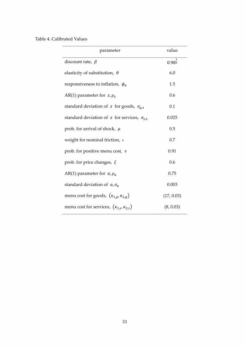
First, we calibrate some parameters at a standard value. Table 4 summarizes our

parameter values. One period in the model corresponds to a quarter, so the discount rate

is set to 0.98 . The elasticity of substitution between goods, , and the

responsiveness of nominal interest rates to inflation, , are set to 6.0 and 1.5, both of

which are conventional values. The disutility of labor supply, , is set to one just as a

normalization.

Then, some of parameters are chosen so that macro moments are consistent with

Japanese data. As described in the previous section, we have the simulated path of

and computed by the model. Thus, the AR(1) parameter and the standard deviation

21

of the discount rate shock, and , are chosen so that the autocorrelation and the

standard deviation of simulated path of are consistent with those of the

Hodrick‐Prescott‐filtered output in Japan. Furthermore, since we can compute the

simulated path of inflation, , by (19) using the simulated path of and , the slope

of the Phillips curve in the model can be obtained by regressing the simulated path of

on that of . While the slope of the Phillips curve is influenced by many parameter

values, one of key determinants is the probability to get chances for price changes, .

Therefore, we choose the value of 0.6 so that the slopes of the Phillips curve under

∗ 1.005 and 0.5 are consistent with Japanese data in the high‐inflation period.

Finally, we calibrate the rest of parameters so that the distributions of price changes

in the model are consistent with that in Japanese data. First, the AR(1) parameter of

idiosyncratic productivity shocks, 0.6 , the standard deviation of idiosyncratic

productivity shocks in a goods sector, , 0.1, and the probability for a positive menu

cost, 0.91, are set to conventional values in the previous literature, including Vavra

(2014). Then, given those conventional values, we choose other parameters by matching

the moments of the distribution of price changes. Regrettably, we have just the

category‐level data for price changes rather than the product‐level data. Therefore, we

compute the distribution of price changes for each category of products. When

computing the category‐level distribution, we assume that the probability to get chances

for price changes, , is decomposed into the category‐level friction, , and the

product‐level friction, . That is, we assume

and ,

where ∈ 0, 1 . Note that each firm has chances for price changes with probability

because . See Appendix for more details about how to compute the

category‐based distribution of price changes.

With the category‐level distribution of price changes in each sector ( ‐distribution,

hereafter), we calibrate seven parameters , , , , , , , , , , , . While each

moment of the ‐distribution is not determined by a single parameter but depends on a

composite of parameters, the rough mapping between the parameter value and the

target moment is as follows: First, the probability for the arrival of idiosyncratic

22

productivity shock, , is chosen by using the interquartile range of the ‐distribution as

a target, because a small leads to a dispersed distribution and vice versa. Then, the

standard deviation of idiosyncratic productivity shocks for the services sector, , , is

chosen by using the interquartile range of the ‐distribution as a target. We choose the

weight between the category‐level friction and the product‐level friction as 0.7, so

that the mass of firms at 1 (i.e., the mass of 0%‐inflation firms) in the

‐distribution is consistent with data. Finally, we choose the parameter for Gamma

distribution of the menu cost , , , , , , , . Considering the shape of Gamma

distribution, we first set to an arbitrary small number , , 0.03 and then

choose , 17 by using the mass of firms at 1 in the ‐distribution as a target.

Then, we choose , 8 to be consistent with the change in the mass of firms at 1

in the ‐distribution when the trend inflation ∗ is changed from 2% to 0%. The change

in the mass of 0%‐inflation firms is closely related to the value of menu cost because the

number of firms in the inaction area is basically determined by the menu cost.

5.2 Simulated Price‐Change Distributions

Figure 8 shows simulated price‐change distributions in goods and services sectors under

2% or 0% trend inflation. The figure indicates that while some moments for the

distribution are used as the calibration targets, the distributions computed by the model

can replicate the changes in the distribution in both sectors along with the decline in

trend inflation in Japan. In the goods sector, as the trend inflation changes from 2% to

0%, the price‐change distribution slides slightly leftward while keeping the weight in the

vicinity of 0% unchanged, reflecting a low menu cost in the goods sector. In the services

sector, the price‐change distribution has more weight in the vicinity of 0% and its

dispersion is narrower under 0% trend inflation than under 2% trend inflation, reflecting

a high menu cost in the services sector.

Furthermore, consistent with the data, while the distribution in the services sector is

highly skewed under 2% trend inflation, it is not skewed under 0% trend inflation.

Under positive trend inflation, firms expect their relative price to continuously become

lower. Hence, given the fact that it is costly to frequently change prices under a high

menu cost, firms in the services sector lose incentive to cut prices under positive trend

23

inflation because they know that their prices will eventually have to increase at some

point in the future. Such a difference in the shape of the distribution under 0% and 2%

trend inflation implies that examining price‐change distributions provides fruitful

information regarding a shift in trend inflation.

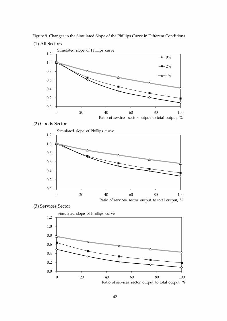
5.3 Slope of the Phillips Curves

Before discussing whether the multisector menu‐cost model can replicate the observed

flattening of the Phillips curve in both goods and services sectors, we first investigate via

comparative statics the influence of declining trend inflation as well as an increasing

share of services in total output on the slope of the Phillips curve. Figure 9 displays the

simulated slope of the Phillips curve under the low, middle, and high trend inflation (i.e.,

0%, 2%, and 4%) by sector, where the horizontal axis represents the ratio of services

sector output to total output (i.e., 0–100%). On one hand, Figure 9 (3) shows that the

Phillips curve in the services sector flattens as trend inflation shifts downward. On the

other hand, Figure 9 (2) indicates that the Phillips curve in the goods sector also flattens

significantly, even though the goods sector bears a much lower menu cost in the model.

These results are consistent with the observed slope of the Phillips curve in the goods

sector. On the influence of increasing the ratio of services sector output to total output,

Figure 9 (2) and (3) show that the rise in share of services makes the Phillips curve flatter

in both goods and services sectors.

Two points are worth noting about the mechanism behind these observations. First,

declining trend inflation makes the services sector reduce the incentives of price changes

due to the existence of the menu cost, leading to an increase in nominal price rigidity in

the services sector. Second, firms in the goods sector set their prices while considering

the relative price of services. Therefore, an increase in price rigidity in the services sector

is likely to reduce the necessity of price changes in the goods sector, too. In this sense,

price rigidity propagates from one sector to others through a relative price effect. The

mechanism is consistent with the observation that under the 0% share of services, slopes

of the Phillips curve on all items (Figure 9 (1)) are almost the same as those in the goods

sector (Figure 9 (2)). These findings imply the importance of examining price‐setting

behaviors in the services sector as well as the goods sector to draw macroeconomic

24

implications because price rigidity in one sector may have a significant effect on the

whole economy.

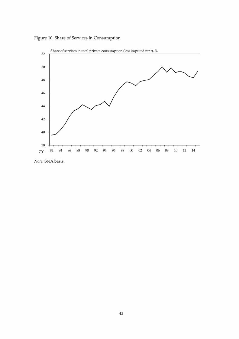
Finally, we compare the simulated and observed slopes of the Phillips curve, taking

into account the changes in both trend inflation and the share of services. Figure 10

provides a view of the development of the share of services in consumption. It shows

that the share of services has increased by about 5–10% from the high‐inflation period of

1982–1994 CY to the low‐inflation period of 1995–2012 CY. Average inflation has also

declined from 2% to 0% during the same period. The simulation based on our menu‐cost

model implies that both changes in trend inflation and share of services decrease the

slope of the Phillips curve by approximately 0.15%, which coincides with the observed

flattening of the Philips curve, as shown in Figure 4. These findings imply that, through

the lens of the menu‐cost model, the flattening of the Phillips curve observed in Japan

can be explained by the decline in trend inflation as well as the rise in share of services.

Therefore, if the Japanese economy returns to positive trend inflation, then the Phillips

curve also would become steeper again. Or, if Japan experiences rises in the proportion

of the share of services in the future, then the Phillips curve would flatten more.

6. Concluding Remarks

Studying Japan’s experience during chronic deflation could be useful in drawing insight

about the relationship between price rigidities and trend inflation. In this paper, we

carried out both empirical and theoretical investigations by employing the menu‐cost

hypothesis. First, we tested plausibility of the menu‐cost hypothesis by estimating the

limited dependent variable model with two‐sided thresholds after controlling for the

other factors such as demand and supply shocks. As a result, we showed higher menu

cost in the services sector than in the goods sector empirically. Second, we constructed a

multisector menu‐cost model in line with the empirical findings and showed that the

model could replicate the shift in the price‐change distributions and changes in the slope

of the Phillips curve in both goods and services sectors. These findings verified that the

menu‐cost hypothesis could consistently explain the series of change in firms’

price‐setting behaviors and macroeconomic consequences on the slope of the Phillips

25

curve during the deflationary period in Japan.

There are some possible research topics for future studies. First, a theoretical

investigation on why the services sector faces higher menu costs is an important work to

complement the analysis in this paper. While this paper empirically validates higher

menu cost in the services sector and takes it as given to investigate a macroeconomic

implication, it is worth investigating which feature in the services sector businesses

entails such a high menu cost. Second, while this paper focuses only on Japan’s

experience, extending this analysis to other countries could be an interesting additional

study. In particular, an increase in the share of services is commonly observed in other

countries too. These can be interesting research topics, but we have left them to be

explored in the future.

26

Appendix

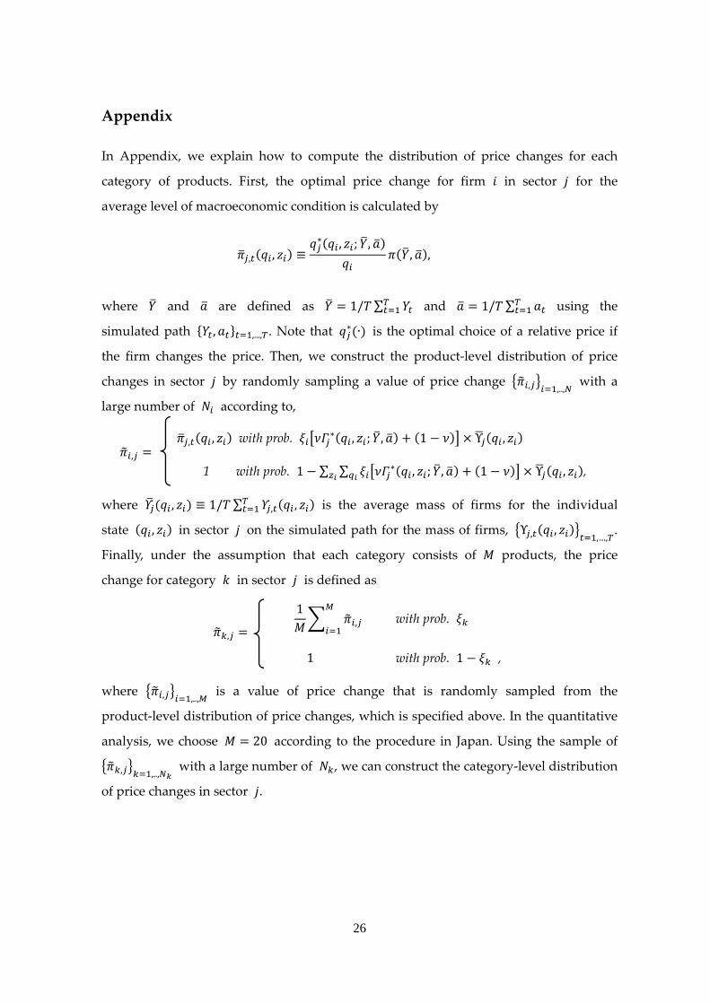
In Appendix, we explain how to compute the distribution of price changes for each

category of products. First, the optimal price change for firm in sector for the

average level of macroeconomic condition is calculated by

, , ≡∗ , ; ,

, ,

where and are defined as 1/ ∑ and 1/ ∑ using the

simulated path , ,..., . Note that ∗ ∙ is the optimal choice of a relative price if

the firm changes the price. Then, we construct the product‐level distribution of price

changes in sector by randomly sampling a value of price change , ,.., with a

large number of according to,

, , , with prob. ∗ , ; , 1 Υ ,

1 with prob. 1 ∑ ∑ ∗ , ; , 1 Υ , ,

where , ≡ 1/ ∑ , , is the average mass of firms for the individual

state , in sector on the simulated path for the mass of firms, Υ , ,,…,

.

Finally, under the assumption that each category consists of products, the price

change for category in sector is defined as

,

1, with prob.

1 with prob. 1 ,

where , ,.., is a value of price change that is randomly sampled from the

product‐level distribution of price changes, which is specified above. In the quantitative

analysis, we choose 20 according to the procedure in Japan. Using the sample of

, ,.., with a large number of , we can construct the category‐level distribution

of price changes in sector .

27

References

Abe, N. and A. Tonogi (2010), “Micro and Macro Price Dynamics in Daily Data,” Journal

of Monetary Economics, 57(6), pp.716–728.

Akerlof, G. A., W. T. Dickens and G. L. Perry (1996), “The Macroeconomics of Low

Inflation,” Brookings Papers on Economic Activity, 1996(1), pp.1–76.

Boivin, J., M. P. Giannoni and I. Mihov (2009), “Sticky Prices and Monetary Policy:

Evidence from Disaggregated Data,” American Economic Review, 99(1), pp.350–84.

Boivin, J., M. T. Kiley and F. S. Mishkin (2010), “How Has the Monetary Transmission

Mechanism Evolved over Time?” Handbook of Monetary Economics, 3, pp.369–422.

Ball, L., N. G. Mankiw and D. Romer (1988), “The New Keynesian Economics and the

Output‐Inflation Trade‐off,” Brookings Papers on Economic Activity, 1, pp.1–65.

Bils, M. and P. J. Klenow (2004), “Some Evidence on the Importance of Sticky Prices,”

Journal of Political Economy, 112(5), pp.947–985.

Caballero, R. J. and E. M. Engel (2007), “Price Stickiness in Ss Models: New

Interpretations of Old Results,” Journal of Monetary Economics, 54(s1), pp.100–121.

Dhyne, E., L. J. Álvarez, H. Le Bihan, G. Veronese, D. Dias, J. Hoffmann, N. Jonker, P.

Lünnemann, F. Rumler and J. Vilmunen (2006), “Price Changes in the Euro Area and

the United States: Some Facts from Individual Consumer Price Data,” Journal of

Economic Perspectives, 20, pp.171–192.

De Veirman, E. (2009), “What Makes the Output‐inflation Trade‐off Change? The

Absence of Accelerating Deflation in Japan,” Journal of Money, Credit and Banking, 41(6),

pp.1117–1140.

Devereux, M. B. and J. Yetman (2002), ʺMenu Costs and the Long‐Run Output‐Inflation

Trade‐Off,ʺ Economics Letters, 76(1), pp.95–100.

Eichenbaum, M., N. Jaimovich and S. Rebelo (2011), “Reference Prices, Costs, and

Nominal Rigidities,” American Economic Review, 101(1), pp.234–62.

Enomoto, H. (2007), “Multi‐Sector Menu Cost Model, Decreasing Hazard, and Phillips

Curve,” Bank of Japan Working Paper Series, No.07–E–3.

28

Gaiotti, E. (2010), “Has Globalization Changed the Phillips Curve? Firm‐level Evidence

on the Effect of Activity on Prices,” International Journal of Central Banking, 6, pp.51–84.

Golosov, M. and R. E. Lucas (2007), “Menu Costs and Phillips Curves,” Journal of Political

Economy, vol.115, pp.171–199.

Higo, M. and Y. Saita (2007), “Price Setting in Japan: Evidence from CPI Micro Data,”

Bank of Japan Working Paper Series, No.07–E–20.

Honoré, B. E., D. Kaufmann and S. Lein (2012), “Asymmetries in Price‐Setting Behavior:

New Microeconometric Evidence from Switzerland,” Journal of Money, Credit and

Banking, 44(s2), pp.211–236.

Kaihatsu, S. and J. Nakajima (2015), “Has Trend Inflation Shifted?: An Empirical

Analysis with a Regime‐Switching Model,” Bank of Japan Working Paper Series,

No.15–E–3.

Kehoe, P. and V. Midrigan (2015), “Prices are Sticky after All,” Journal of Monetary

Economics, 75, pp.35–53.

Kiley, M. T. (2000), “Endogenous Price Stickiness and Business Cycle Persistence,”

Journal of Money, Credit and Banking, 32(1), pp.28–53.

Kimura, T. and T. Kurozumi (2010), ʺEndogenous Nominal Rigidities and Monetary

Policy,ʺ Journal of Monetary Economics, 57(8), pp. 1038–1048.

Klenow, P. J and O. Kryvtsov (2008), “State‐Dependent or Time‐Dependent Pricing:

Does It Matter for Recent U.S. Inflation?,” Quarterly Journal of Economics,123(3),

pp.863–904.

Kurachi, Y., K. Hiraki, and S. Nishioka (2016), “Does a Higher Frequency of Micro‐Level

Price Changes Matter for Macro Price Stickiness? Assessing the Impact of Temporary

Price Changes,” Bank of Japan Working Paper Series, No.16–E–9.

Kuroda, S. and I. Yamamoto (2003), “The Impact of Downward Nominal Wage Rigidity

on the Unemployment Rate: Quantitative Evidence from Japan,” Monetary and

Economic Studies, 21(4), pp.57–85.

Kurozumi, T. (2016), ʺEndogenous Price Stickiness, Trend Inflation, and Macroeconomic

29

Stability,ʺ Journal of Money, Credit and Banking, 48(6), pp.1267–1291.

Krusell, P. and A. A. Smith, Jr. (1998), “Income and Wealth Heterogeneity in the

Macroeconomy,” Journal of Political Economy, 106(5), pp.867–896.

Levin, A. and T. Yun (2007), ʺReconsidering the Natural Rate Hypothesis in a New

Keynesian Framework,ʺ Journal of Monetary Economics, 54(5), pp.1344–1365.

Midrigan, V. (2011), “Menu Costs, Multiproduct Firms, and Aggregate Fluctuations,”

Econometrica, 79(4), pp.1139–1180.

Nakamura, E. and J. Steinsson (2008), “Five Facts about Prices: A Reevaluation of Menu

Cost Models,” Quarterly Journal of Economics, 123(4), pp.1415–1464.

Nakamura, E. and J. Steinsson (2010), “Monetary Non‐Neutrality in a Multi‐Sector Menu

Cost Model,” Quarterly Journal of Economics, 125(3), pp.961–1013.

Nakamura, E. and J. Steinsson (2013), “Price Rigidity: Microeconomic Evidence and

Macroeconomic Implications,” Annual Review of Economics, 5(1), pp.133–163.

Romer, D. (1990), ʺStaggered Price Setting with Endogenous Frequency of Adjustment,ʺ

Economics Letters, 32(3), pp.205–210.

Rosett, R. (1959), “A Statistical Model of Friction in Economics,” Econometrica, 27(2),

pp.263–267.

Sekine, T. and T. Tachibana (2004), “Land Investment by Japanese Firms during and

after the Bubble Period,” Bank of Japan Working Paper Series, No.04–E–2.

Sudo, N., K. Ueda and K. Watanabe (2014), “Micro Price Dynamics During Japanʹs Lost

Decades,” Asian Economic Policy Review, 9(1), pp.44–64.

Train, K. (2003), “Discrete Choice Methods with Simulation,” Cambridge University

Press, Cambridge.

Vavra, J. (2014), “Inflation Dynamics and Time‐Varying Volatility: New Evidence and an

Ss Interpretation,” Quarterly Journal of Economics, 129(1), pp.215–258.

Watanabe, K. and T. Watanabe (2017), “Price Rigidity at Near‐Zero Inflation Rates:

Evidence from Japan,” CARF Working Papers, F–408.

30

Table 1. Series Description in the Dataset

Category Classification

Productions by goods

Shipments by goods

Inventories by goods

Inventory Ratio by goods

Utilization Ratio by industry

Indices of Tertiary Industry

Activityby industry

Machinery Orders Statistics Total Value of Machinery Order by sectors

Floor Area by use types

Planned Amount of Construction

Costsby use types

Number of Buildings by use types

Monthly Bankruptcy Report Number of Bankruptcy

Electricity Demand Electricity Demand by sectors

Producer Price Index by groups

Export Price Index by groups

Import Price Index by groups

Services Producer Price Index by groups

Nikkei Commodity Price

Indexby goods

Oil Price Brent Crude Oil Price

Scheduled Cash Earnings by industry

Total Hours Worked by industry

Non‐scheduled Hours Worked by industry

Number of Regular Employee by industry

Number of Employed Persons

Number of Unemployed Persons

Report on Employment

Service

Number of Job Offers and Job

Seekers

Employment Insurance

StatisticsInsured Workers

New Car Registration Number of sales by vehicle classification

Family Income and

Expenditure SurveyConsumption expenditure by items

Current Survey of Commerce Sales value by industry

GovernmentIntegrated Statistics on

Construction Works

Amount of public construction

completed

Export Volume Index by goods

Import Volume Index by goods

Terms of Trade Index

Money Stock M2

Nominal Effective Exchange Rate

Real Effective Exchange Rate

Stock Prices Tokyo Stock Price Index by scales

Interest Rate Overnight Call Rate

Labor Market

Labor Statistics

Labor Force Survey

Statistics

Corporate

Activity

Indices of Industrial

Production

Statistics on Building

Construction Starts

Price

Corporate Goods Price Index

Household

Trade Trade Statistics

Money and

Financial

Market

Foreign Exchange

31

Table 2. Estimation Results of the Friction Model (Consumer Price Index)

Note: The standard errors for estimates are presented in parenthesis.

*** denotes significance at the 1% level.

θ ‐ 1.52 (0.01) *** 0.40 (0.01) *** 3.54 (0.01) ***

θ + 1.36 (0.01) *** 1.34 (0.01) *** 1.33 (0.01) ***

β 1 0.92 (0.00) *** 0.95 (0.00) *** 0.89 (0.01) ***

β 2 0.72 (0.01) *** 1.10 (0.01) *** 0.15 (0.01) ***

Consumption tax rate 0.64 (0.01) *** 0.39 (0.01) *** 0.96 (0.01) ***

σ 6.48 (0.05) *** 6.12 (0.07) *** 6.80 (0.08) ***

Observations

CPI (All items, less fresh

food and imputed rent)

CPI (Goods, less

fresh food)

CPI (Services, less

imputed rent)

140,241 103,348 36,893

32

Table 3. Estimation Results of the Friction Model (Retail Price Survey)

Note: The standard errors for estimates are presented in parenthesis.

*** denotes significance at the 1% level.

θ ‐ 12.65 (0.07) *** 18.37 (0.09) ***

θ + 16.48 (0.07) *** 15.99 (0.08) ***

β 1 2.47 (0.04) *** 2.88 (0.05) ***

β 2 0.65 (0.07) *** 2.40 (0.07) ***

Consumption tax rate 2.76 (0.11) *** 0.96 (0.12) ***

σ 20.44 (0.26) *** 15.26 (0.46) ***

Observations

RPS (Goods, less fresh food) RPS (Services, less imputed rent)

201,216 107,648

33

Table 4. Calibrated Values

parameter value

discount rate, 0.98

elasticity of substitution, 6.0

responsiveness to inflation, 1.5

AR(1) parameter for , 0.6

standard deviation of for goods, , 0.1

standard deviation of for services, , 0.025

prob. for arrival of shock, 0.5

weight for nominal friction, 0.7

prob. for positive menu cost, 0.91

prob. for price changes, 0.6

AR(1) parameter for , 0.75

standard deviation of , 0.003

menu cost for goods, , , , (17, 0.03)

menu cost for services, , , , (8, 0.03)

34

Figure 1. Median and the First/Third Quantile Points of the Price‐Change Distribution

Note: All the series are averages weighted by the CPI weight.

(1) CPI (All items, less fresh food and imputed rent)

(2) CPI (Goods, less fresh food)

(3) CPI (Services, less imputed rent)

‐6

‐4

‐2

0

2

4

6

8

82 85 88 91 94 97 00 03 06 09 12 15

YoY, %

CY

‐6

‐4

‐2

0

2

4

6

8

82 85 88 91 94 97 00 03 06 09 12 15

First quantile (25th percent)

Median

Third quantile (75th percent)

YoY, %

CY

‐6

‐4

‐2

0

2

4

6

8

82 85 88 91 94 97 00 03 06 09 12 15

YoY, %

CY

35

Figure 2. Frequency of Price Adjustments

Note: ʺPrice changeʺ is defined as a quarterly change more than ±0.1% in the item level.

Figures show yearly averages of monthly frequency, calculated by dividing the

number of items whose prices change by the number of total items in each month.




20

30

40

50

60

70

82 85 88 91 94 97 00 03 06 09 12

%

FY

20

30

40

50

60

70

82 85 88 91 94 97 00 03 06 09 12

%

FY

20

30

40

50

60

70

82 85 88 91 94 97 00 03 06 09 12

%

FY

36

Figure 3. Price‐Change Distributions in the High‐ and Low‐Inflation Periods

Note: Figures are calculated based on quarterly‐based inflation rate.


<High‐inflation period (1982‐94FY)> <Low‐inflation period (1995‐2012FY)>


<High‐inflation period (1982‐94FY)> <Low‐inflation period (1995‐2012FY)>

0

10

20

30

40

50

60

70

‐4 ‐3 ‐2 ‐1 0 1 2 3 4

Relative frequency, %

%

0

10

20

30

40

50

60

70

‐4 ‐3 ‐2 ‐1 0 1 2 3 4


%

0

10

20

30

40

50

60

70

‐4 ‐3 ‐2 ‐1 0 1 2 3 4


%

0

10

20

30

40

50

60

70

‐4 ‐3 ‐2 ‐1 0 1 2 3 4%


37

Figure 4. Phillips Curve

Note: The standard errors for estimates are presented in the parenthesis.

For the Hodrick‐Prescott filter, we set the smoothing parameter to 1600.




y = 0.49 x + 2.11

y = 0.34 x ‐ 0.19

‐3

‐2

‐1

0

1

2

3

4

‐8 ‐6 ‐4 ‐2 0 2 4 6

High‐inflation period (1982‐94FY)Low‐inflation period (1995‐2012FY)

GDP, deviation from the HP‐filtered trend, 2‐quarter lead,%

(0.07)

(0.04)

YoY, %

y = 0.66 x + 1.70

y = 0.51 x ‐ 0.47

‐4

‐3

‐2

‐1

0

1

2

3

4

5

‐8 ‐6 ‐4 ‐2 0 2 4 6

YoY, %

(0.10)

(0.06)

GDP, deviation from the HP‐filtered trend, 2‐quarter lead, %

y = 0.21 x + 2.74

y = 0.11 x + 0.18

‐2

‐1

0

1

2

3

4

5

‐8 ‐6 ‐4 ‐2 0 2 4 6GDP, deviation from the HP‐filtered trend, 2‐quarter lead, %

(0.07)

（0.04）

YoY, %

38

Figure 5. Median and the First/Third Quantile Points of the Distribution of Firm‐level

Wage Cost

‐10

‐8

‐6

‐4

‐2

0

2

4

6

8

10

82 84 86 88 90 92 94 96 98 00 02 04 06 08 10 12

First quantile

Median

Third quantile

YoY, %

CY

39

Figure 6. A Limited Dependent Variable Model with Two‐sided Thresholds

0

40

Figure 7. Price‐Change Distributions Based on the Retail Price Survey

<Goods, less fresh food> <Services>

0

10

20

30

40

50

60

70

80

‐50 ‐40 ‐30 ‐20 ‐10 0 10 20 30 40 50


YoY, %

0

10

20

30

40

50

60

70

80

‐50 ‐40 ‐30 ‐20 ‐10 0 10 20 30 40 50YoY, %


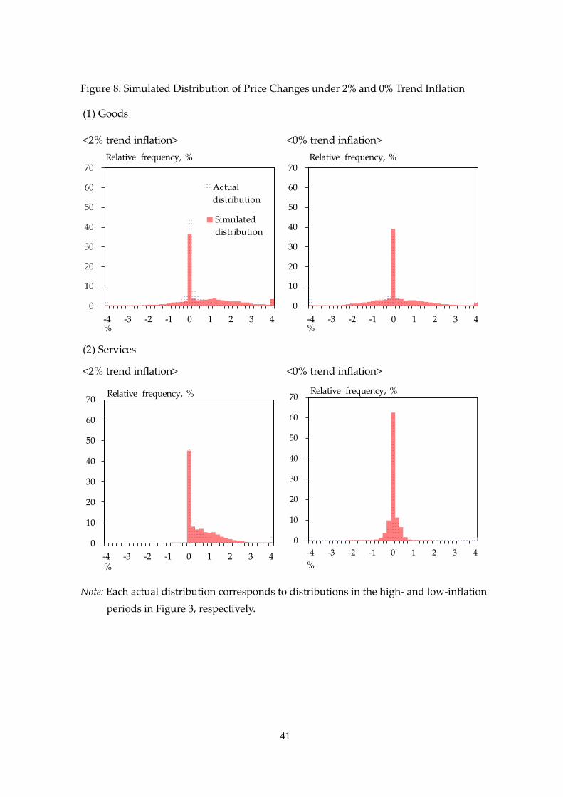
Figure 8. Simulated Distribution of Price Changes under 2% and 0% Trend Inflation

Note: Each actual distribution corresponds to distributions in the high- and low-inflation

periods in Figure 3, respectively.

(1) Goods

<2% trend inflation> <0% trend inflation>

(2) Services

<2% trend inflation> <0% trend inflation>

Actualdistribution

0

10

20

30

40

50

60

70

-4 -3 -2 -1 0 1 2 3 4%


0

10

20

30

40

50

60

70

-4 -3 -2 -1 0 1 2 3 4

Simulateddistribution

%


0

10

20

30

40

50

60

70

-4 -3 -2 -1 0 1 2 3 4%


0

10

20

30

40

50

60

70

-4 -3 -2 -1 0 1 2 3 4%


41

42

Figure 9. Changes in the Simulated Slope of the Phillips Curve in Different Conditions

(1) All Sectors

(2) Goods Sector

(3) Services Sector

0.0

0.2

0.4

0.6

0.8

1.0

1.2

0 20 40 60 80 100

0%

2%

4%

Simulated slope of Phillips curve

Ratio of services sector output to total output, %

0.0

0.2

0.4

0.6

0.8

1.0

1.2

0 20 40 60 80 100



0.0

0.2

0.4

0.6

0.8

1.0

1.2

0 20 40 60 80 100



43

Figure 10. Share of Services in Consumption

Note: SNA basis.

38

40

42

44

46

48

50

52

82 84 86 88 90 92 94 96 98 00 02 04 06 08 10 12 14

Share of services in total private consumption (less imputed rent), %

CY

Phillips Curve and Price‐Change Distribution under .... Phillips Curve and Price‐Change...

Documents

Transcript of Phillips Curve and Price‐Change Distribution under .... Phillips Curve and Price‐Change...

Phillips Curve Macroeconomics Cunningham. 2 Original Phillips Curve A. W. Phillips (1958), “The Relation Between Unemployment and the Rate of Change of.

The New Keynesian Phillips curve: a critical … The New Keynesian Phillips curve: a critical assessment Gabriel Aidar* ABSTRACT Two main versions of the Phillips curve can be found

The Modern Phillips Curve Revisited · Phillips Curve; Business Cycle; Inflation; Unemployment 1. Introduction The modern Phillips curve is about the relationship between the average

The Phillips Curve - Zentraler Informatikdienst » …homepage.univie.ac.at/christina.zauner/Phillips Curve.pdfThe Phillips Curve Christina Zauner Introduction Derivation of the Phillips

Phillips Curve and Wage Inflation Dynamics · Phillips Curve and Wage Inflation Dynamics Abstract: Debates around the Phillips curve, a long-time relationship between unemployment

The Phillips Curve

The Phillips Curve and Expectations Theory

Stability of the Phillips Curve

Phillips Curve - Bronx High School of Science Curve.pdfInflation and Unemployment: The Phillips Curve The Short-Run Phillips Curve We've just seen that expansionary policies lead to

Inflation and phillips curve

Phillips Curve - University of Connecticutweb.uconn.edu/cunningham/econ309/phillipscurve.pdf · 2 Original Phillips Curve zA. W. Phillips (1958), “The Relation Between Unemployment

CHAPTER 16 Analysis of AS curve Analysis of AS curve Phillips curve Phillips curve Supply shocks Supply shocks Laffer curves Laffer curves.

Inflation Theories , Unemloyment & Phillips Curve

The Long-Run Phillips Curve is a Curve 1

Phillips Curve Mc and Answers

The History of the Phillips Curve - NZAE€¦ · The History of the Phillips Curve: An American Perspective ABSTRACT This history of the Phillips Curve adopts an American perspective,

Phillips Curve Inflation Forecasts - Princeton Universitymwatson/papers/PhillipsCurveInflation... · Phillips Curve Inflation Forecasts . ... conclusion concerning Phillips curve

© 2007 Thomson South-Western Phillips Curve. © 2007 Thomson South-Western The Phillips Curve Phillips Curve (PC)– relationship between Inflation and Unemployment.

Phillips Curve Lithuania

PHILLIPS CURVE. Phillips Curve Short and Long Run Phillips Curves William Phillips, a New Zealand born economist, wrote a paper in 1958 titled The Relation.