© 2006 International Monetary Fund May 2006

IMF Country Report No. 06/181

Philippines: Selected Issues

This Selected Issues paper for the Philippines was prepared by a staff team of the International Monetary Fund as background documentation for the periodic consultation with the member country. It is based on the information available at the time it was completed on January 30, 2006. The views expressed in this document are those of the staff team and do not necessarily reflect the views of the government of the Philippines or the Executive Board of the IMF. The policy of publication of staff reports and other documents by the IMF allows for the deletion of market-sensitive information.

To assist the IMF in evaluating the publication policy, reader comments are invited and may be sent by e-mail to publicationpolicy@imf.org.

Copies of this report are available to the public from

International Monetary Fund ● Publication Services 700 19th Street, N.W. ● Washington, D.C. 20431

Telephone: (202) 623 7430 ● Telefax: (202) 623 7201 E-mail: publications@imf.org ● Internet: http://www.imf.org

Price: $15.00 a copy

International Monetary Fund

Washington, D.C.

INTERNATIONAL MONETARY FUND

PHILIPPINES

Selected Issues

Prepared by Robin Brooks, Kotaro Ishi (APD), Srikant Seshadri (PDR) and Daria Zakharova (FAD)

Approved by Asia and Pacific Department

January 30, 2006

Contents Page I. What Lies Behind the Diminished Volatility of Philippines Sovereign Debt?.............................................................................................4 A. Introduction and Background ........................................................................4 B. Diminished Volatility of RoPs Has Coincided With Increased Domestic Ownership......................................................................................6 C. What has Driven the Demand for RoPs by Philippine Banks?......................6 D. Why Might a Philippine Asset Manager Find RoPs Desirable?....................7 E. Summary and Conclusions ..........................................................................10 II. Cyclically-Adjusted Balances and Fiscal Sustainability in the Philippines..........11 A. Introduction .................................................................................................11 B. Methodology................................................................................................12 C. Findings........................................................................................................13 D. Making Fiscal Consolidation a Success.......................................................18 III. Explaining Economic Growth in The Philippines ................................................25 A. Introduction .................................................................................................25 B. Philippines’ Growth Performance................................................................25 C. Explaining Growth in The Philippines ........................................................27 D. Growth Regressions .....................................................................................32 E. Conclusions .................................................................................................34 IV. Second-Round Effects of the Oil Shock on Inflation ...........................................44 A. Introduction .................................................................................................44 B. Recent Inflation Developments....................................................................45 C. Measures of Core Inflation ..........................................................................46 D. Choosing Among Measures of Core Inflation.............................................48 E. Second-Round Effects From the Oil Shock.................................................49 F. Conclusions .................................................................................................50

- 2 -

Contents Page Boxes II-1. National Government Tax Revenue Developments in l990-2004........................15 II-2. International Comparison of Revenues and Expenditures....................................20 Figures I-1. Emerging Market Bond Spreads and the Philippines Sub-Index............................4 I-2. Bonds as a Share of Philippines External Debt ......................................................5 I-3. Volatility................................................................................................................. 6 I-4. Domestic Investor Holdership of RoPs...................................................................6 I-5. Foreign Currency Deposits, Foreign Currency Lending to Residents and RoP

Ownership ...............................................................................................................6 I-6. Comparative Cumulative Returns on RoPs versus Peso Bonds .............................8 I-7. The Philippine Peso ................................................................................................8 II-1. Nonfinancial Public Sector Deficit and Debt........................................................11 II-2. Cyclically Adjusted Balance and Output Gaps.....................................................14 II-3. National Government Tax Revenue and Statutory Outlays..................................16 II-4. National Government Expenditure Composition..................................................17 II-5. Tax Revenues in the Philippines and Comparator Countries ...............................22 II-6. Expenditures in the Philippines and Comparator Countries .................................23 III-1. Real per Capita GDP Growth ...............................................................................25 III-2. GDP per Capita .....................................................................................................26 III-3. Labor Productivity ................................................................................................27 III-4. Economic Policy Indicators ..................................................................................29 III-5. Governance Indicators ..........................................................................................31 III-6. Legal System and Property Rights Indicators.......................................................32 III-7. Political Risk and Constraints on Executives .......................................................32 III-8. Per Capita GDP Level: Actual vs. Prediction.......................................................33 III-9. Per Capita GDP Growth: Actual vs. Prediction....................................................33 III-10. GDP per Worker Growth: Actual vs. Prediction ..................................................34 IV-1. Headline Inflation .................................................................................................45 IV-2. Contributions to Headline Inflation ......................................................................45 IV-3. One-Year-Ahead Inflation Expectations...............................................................46 IV-4. Explanatory Power (R2) of Core Inflation Measures............................................49 Text Tables I-1. The Structure of Philippine External Debt..............................................................5 I-2. Comparison of Quarter-on-Quarter Returns on RoPs Versus Peso-Denominated Government Bonds..................................................................8 I-3. Summary Results of Event Study ...........................................................................9

- 3 -

III-1. GDP and Population Growth ................................................................................25 III-2. Growth Accounting...............................................................................................27 III-3. Geography .............................................................................................................28 III-4. What are Predicted Increases in Growth Rates? ...................................................35 IV-1. M/M Inflation in Percent .....................................................................................48 IV-2. Additions to y/y Headline and Core Inflation Rates.............................................50 Annexes III-1. The Regression Exercise.......................................................................................36 III-2. Data Used in the Regression Exercise ..................................................................39 IV-1. Technical Annex .................................................................................................51

- 4 -

Figure 1. EMBIG Spreads and the EMBIG Philippines Sub-index

200

300

400

500

600

700

800

900

1000

1100

1200

1/3/

2000

4/3/

2000

7/3/

2000

10/3

/200

0

1/3/

2001

4/3/

2001

7/3/

2001

10/3

/200

1

1/3/

2002

4/3/

2002

7/3/

2002

10/3

/200

2

1/3/

2003

4/3/

2003

7/3/

2003

10/3

/200

3

1/3/

2004

4/3/

2004

7/3/

2004

10/3

/200

4

1/3/

2005

4/3/

2005

7/3/

2005

10/3

/200

5

EMBIG OverallEMBIGPhilippines

Pres.Arroyosworn in

Argentina Brazil/ENRONFed startsraising ratesPresident Arroyo

sworn in Sin taxes,Mining Ruling

EVATPhase I

I. WHAT LIES BEHIND THE DIMINISHED VOLATILITY OF PHILIPPINES SOVEREIGN DEBT?1

A. Introduction and Background

1. In 2005, the Philippines was one of the strongest performers in emerging debt markets. Republic of Philippines bonds (RoPs) returned over 20 percent in 2005—nearly twice the return on the EMBI-Global. One of the remarkable features of this performance is the fact that the Philippines component of the EMBI-Global returned some 19 percent (annualized) during both the second and the third quarters, when the country weathered a period of considerable political turbulence. This chapter examines some of the factors that lie behind the stability in the performance of Philippine bonds, and whether this is likely to endure. It is tempting to believe that the diminished volatility of Philippine bonds is merely a reflection of what has happened in the broader market; indeed in all credit markets since 2003, abundant global liquidity has driven the search for yield, re-priced credit risk, and brought with it a sharp decline in volatility. Such reasoning would imply that the diminished volatility is only as enduring as the accommodative global conditions. While global factors have certainly played a role in the dynamics of Philippines debt, this chapter argues that there are also significant Philippines-specific factors at work. Analyses of the sustainability of this “lower-volatility” regime must take such factors into account. Principally, the chapter points to the fact that the ownership of Philippines bonds has been changing markedly over the last two to three years. So long as these trends in ownership are maintained, the sensitivity to global conditions may not be as strong as in the past.

2. Prior to examining these factors, it is useful to establish a number of stylized facts regarding Philippine external debt. Philippine external debt is estimated at 68 percent of GDP,2 roughly two-thirds of which is owed by the public sector. The general structure of this debt has been very stable. The share of short-term debt (as of June 2005, estimated at 10.9 percent) has remained in a very tight range between 9 percent and 12 percent over the

1 Prepared by Srikant Seshadri (sseshadri@imf.org).

2 Gross of domestic holdership, and including estimates of the “non-monitored” debt stock.

- 5 -

Figure 2. Bonds as a Share of Philippine External Debt (%)

20.0

22.0

24.0

26.0

28.0

30.0

32.0

34.0

36.0

38.0

40.0

Dec-99

Apr-00

Aug-00

Dec-00

Apr-01

Aug-01

Dec-01

Apr-02

Aug-02

Dec-02

Apr-03

Aug-03

Dec-03

Apr-04

Aug-04

Dec-04

Apr-05

Total

Public Sector

Table 1. The Structure of Philippine External Debt

Share of S.T. Debt

(Percent)

Share of Variable Rate MLT Debt

(Percent)

Average Rate on Fixed Rate Debt

(Percent)

Public External Debt Weighted

Average Maturity (Years)

Dec-99 9.7 38.8 5.42 19.9 Dec-00 10.7 42.8 5.82 19.4 Dec-01 11.6 44.9 5.98 19.0 Dec-02 10.4 40.4 6.11 19.1 Dec-03 10.8 39.5 6.04 19.4 Dec-04 9.2 35.1 5.74 19.6 Mar-05 10.0 34.1 5.96 20.0 Jun-05 10.9 34.6 6.09 19.9

last six years. The medium-and long-term debt has a long weighted average life of 17.6 years (close to 20 years for public sector debt), and this too has remained within a tight range over the last several years. Through skillful management, the Philippine authorities have exploited the low interest rate environment to bring down the share of variable rate debt by over 10 percent since 2001 to around 35 percent of the total, while at the same time keeping the average interest rate of the fixed rate debt more or less constant at around 6 percent.

3. A noteworthy trend in the last several years has been an increased reliance on external commercial financing. The share of official creditors has become correspondingly smaller, with the share of banks and financial institutions remaining roughly constant at about one-fifth. The share of debt owed to bond and noteholders has risen, both for the private and public sectors. As of June 2005, there were some $28 billion of outstanding bonds, of which $19 billion is owed by the national government. Bond holders currently hold over 30 percent of the external debt, and close to 40 percent of the public sector’s external debt. Of the $28 billion in bonds, some $10 billion is held by domestic residents. The largest holders of domestically held debt are local banks (estimated at 81 percent), and insurance companies and pension funds (14 percent), with the latter two doubling their share over the last six years. Around $7 billion of the domestically held bonds are thought to be sovereign bonds, with the rest issued by other entities.

- 6 -

Figure 3. Volatility (bps) has Diminished Markedly

30

35

40

45

50

55

60

65

70

75

80

2000 2001 2002 2003 2004 20056

7

8

9

10

11

12

13

14

15

Total Return Volatility (LHS)

Spread Volatility (RHS)

Figure 4. Domestic Investor Holdership of RoPs (%)

20.0

25.0

30.0

35.0

40.0

45.0

Mar-00

Jun-00

Sep-00

Dec-00

Mar-01

Jun-01

Sep-01

Dec-01

Mar-02

Jun-02

Sep-02

Dec-02

Mar-03

Jun-03

Sep-03

Dec-03

Mar-04

Jun-04

Sep-04

Dec-04

Mar-05

Jun-05

Sep-05

Figure 5. FCDUs, Foreign Currency Lending to Residents and RoP Ownership ($ billions)

10

11

12

13

14

15

16

17

18

19

Dec-99

Mar-00

Jun-00

Sep-00

Dec-00

Mar-01

Jun-01

Sep-01

Dec-01

Mar-02

Jun-02

Sep-02

Dec-02

Mar-03

Jun-03

Sep-03

Dec-03

Mar-04

Jun-04

Sep-04

Dec-04

Mar-05

Jun-05

0

1

2

3

4

5

6

7

8

9

Domestic ownership of RoPs (RHS)

FCDU Deposits (LHS)

FC Lending to Residents (RHS)

B. Diminished Volatility of RoPs Has Coincided With Increased Domestic Ownership

4. Over the past six years, the Philippines has been through a period of considerable uncertainty regarding the course of economic policy, and has suffered a series of adverse rating actions. With the implementation of the first phase of the VAT reform law in November 2005, such concerns have begun to dissipate, but the turbulence of the preceding period is reflected by the weakening of the peso (by over 30 percent since January 2000). In the third quarter of 2005, when the currency plumbed new lows against the dollar, RoPs performed strongly. As the figures show, this represents the continuation of a broader trend towards lower volatility, which has also been accompanied by a marked rise in the domestic ownership of RoPs. It therefore seems reasonable to attribute part of the stability of the bonds to the fact that they seem to have found “steadier” hands, and not just to sanguine global conditions.3

C. What has Driven the Demand for RoPs by Philippine Banks?

5. As previously noted, Philippine banks are estimated to hold over 80 percent of domestically held external bonds. This share has risen from a little over 70 percent in 1999. The driving factors behind the increase in domestic holdership of RoPs must therefore be traced back to banks’ behavior. There are two concurrent drivers of the banking sector’s bid for RoPs. First, in the aftermath of the Asian crisis, there has been a secular decline in foreign currency denominated lending to the private sector (though this has partially changed recently with a pick up in lending to some of the stronger performing companies, particularly telecoms). For the level of credit risk, banks, which have been awash with cash

3 Preliminary data from the central bank show that in 2004, domestic investors purchased over $3 billion of externally floated Philippine debt, or close to a fifth of the entire stock of RoPs, from external investors in the secondary market alone.

- 7 -

over the last two years, appear to be more comfortable with RoPs. Second, and just as important, starting in 2004, there was a strong rise in foreign currency deposits by residents (almost exclusively in dollars), and banks needed to match these liabilities with dollar denominated assets.4

6. The forces behind increased bank holdings of RoPs deserve some scrutiny. After remaining in a tight range between $12.9–$13.4 billion during 2001–03, foreign currency deposits have risen markedly in recent years; from end-2003 to September 2005, deposits held by Foreign Currency Deposit Units5 (FCDUs) rose by nearly $2.4 billion. Despite this additional funding, foreign currency lending by FCDUs contracted over this period, falling from $3.5 billion at end-2003 to $3.0 billion in September 2005. Given the currency matching requirements, banks have therefore had to seek alternative foreign currency assets. Some of this demand has been met by increased interbank loans to foreign banks and U.S. Treasury instruments, but clearly RoPs also have been a major beneficiary. This period also coincides with the period when banks increased their exposure to credit derivatives based on RoP risk. In addition to $7 billion of sovereign bonds that is domestically held, market estimates suggest that financial institutions’ implicit “long” position on RoPs is further enhanced by $1–1.5 billion of credit derivatives.

D. Why Might a Philippine Asset Manager Find RoPs Desirable?

7. It is instructive to look at how a bond manager in the Philippines, choosing between peso denominated government bonds and RoPs would have fared over the last six years. The bond manager does not face the same currency matching requirements as a bank, and is therefore relatively unconstrained in asset allocation choices. In a very stylized fashion, it is possible to demonstrate that RoPs have been a superior investment over the last six years. Figure 6 compares the cumulative value of an investment in RoPs (as measured by the Philippines sub-component of the EMBI-Global) with that of an investment in five-year peso denominated government bonds (in dollar terms), assuming a 100 percent reinvestment rate. The cumulative returns on peso bonds are some 40 percent lower over this period, primarily because the of the performance of the peso (Figure 7), not because of the performance of the bonds per se. Table 2 shows a comparison of quarter-on quarter total

4 These banks could, of course, purchase other dollar denominated assets, but the existence of a strong “home bias” is common knowledge in the Philippines, and is in fact, widely prevalent globally in the asset allocation process (see Global Financial Stability Reports April 2004, and September 2005). While there are other equally high yielding instruments as RoPs, domestic banks frequently cite two factors as drivers of this home bias: First, their familiarity with Philippines risk, and second, an institutional aversion to other more complicated financial instruments which might offer comparable yields. Additionally, as Philippine bonds are zero-risk weighted per banking regulations, this also creates a natural advantage for RoPs. 5 The FCDU data from the BSP covers both resident and non-resident lending and deposits.

- 8 -

Figure 6. Comparative Cumulative Returns on RoPs versus Peso Bonds

80.0

90.0

100.0

110.0

120.0

130.0

140.0

150.0

160.0

170.0

180.0

190.0

200.0

210.0

Jan-00

Apr-00

Jul-00

Oct-00

Jan-01

Apr-01

Jul-01

Oct-01

Jan-02

Apr-02

Jul-02

Oct-02

Jan-03

Apr-03

Jul-03

Oct-03

Jan-04

Apr-04

Jul-04

Oct-04

Jan-05

Apr-05

Jul-05

Oct-05

RoPs

Peso bonds

Figure 7. The Philippine Peso (PHP/USD)

40

42

44

46

48

50

52

54

56

58

1/3/

2000

4/3/

2000

7/3/

2000

10/3

/200

0

1/3/

2001

4/3/

2001

7/3/

2001

10/3

/200

1

1/3/

2002

4/3/

2002

7/3/

2002

10/3

/200

2

1/3/

2003

4/3/

2003

7/3/

2003

10/3

/200

3

1/3/

2004

4/3/

2004

7/3/

2004

10/3

/200

4

1/3/

2005

4/3/

2005

7/3/

2005

10/3

/200

5

returns on RoPs versus peso denominated bonds. Over the period from 2000–05, on average, RoPs have performed better on an absolute and risk-adjusted basis.

Table 2. Comparison of Quarter-on-Quarter Returns on RoPs versus Peso-Denominated Government Bonds (January 2000–December 2005)

RoPs Peso-bonds

Mean quarterly return (percent) 3.10 Mean quarterly return (percent) 2.23 Standard deviation of returns 4.29 Standard deviation of returns 5.68 Return per standard deviation (percent) 0.72 Return per standard deviation (percent) 0.39

8. In order to more carefully compare the performance of RoPs against five-year peso-denominated bonds particularly during periods of turbulence, an elementary event study was performed for the period January 2000 to September 2005. An “event” was defined as an adverse occurrence which caused a minimum week-long sell-off in either or both: (a) the peso (with a threshold weakening by at least two-thirds of the weekly standard deviation of the currency moves); (b) the Philippines EMBI-Global sub-component (with a threshold spread widening of at least two-thirds of a weekly standard deviation of spread moves). The universe of possible “events” includes political uncertainty, uncertainty associated with policy legislation, adverse reactions to unfavorable data releases, rating agency downgrades, as well as externally driven events such as the Argentine default, or the period of dislocation immediately after September 11, 2001. Using this definition, 17 “events” were identified in the specified period. The average duration of an “event” was 66 days with a standard deviation of 82 days.6 RoPs outperformed the five-year peso bond in

6 We treated the whole of the year 2000 as a single event, to prevent excessive clustering. Excluding this year, the average duration drops to 47 days, and the standard deviation about this average is 42 days.

- 9 -

12 out of these 17 “events”.7 The average outperformance (annualized) was 9.27 percent. In the 5 events where the peso asset was the stronger performer, its outperformance averaged 29.4 percent, whereas in the events where RoPs were the stronger performer, the average outperformance was 25.4 percent.8 The results are summarized in the table below.

Table 3. Summary Results of Event Study

Event Period RoP Returns

(Annualized, Percent) Peso Bonds Returns

(in US$, Annualized, Percent)

January–December 2000 -2.50 -23.99 02/15/01–04/30/01 6.18 -51.86 06/01/01–08/06/01 2.63 -12.33 09/11/01–09/26/01 -30.80 2.80 10/22/01–11/02/01 -36.70 3.60 12/21/01–01/07/02 21.20 -10.70 05/21/02–06/25/02 -20.60 30.88 07/22/02–03/17/03 4.52 -3.80 05/15/03–06/18/03 66.50 -14.05 07/01/03–08/26/03 -17.60 -11.90 10/20/03–11/28/03 -33.60 -17.80 01/09/04–03/25/04 -3.26 -14.18 06/08/04–06/29/04 -1.70 -8.70 08/23/04–10/14/04 6.20 3.33 05/09/05–07/13/05 5.00 -10.30 07/25/05–08/03/05 13.46 -17.80 08/21/05–09/27/05 24.20 2.30 Average 0.18 -9.09

9. Such an event study has the inherent methodological limitation that it is conducted with the benefit of hindsight, while an asset manager’s decisions are forward-looking. Therefore, the results of this study cannot be construed as concrete evidence that an asset manager would have had a definitive preference for RoPs over domestic bonds. Nonetheless, the study is suggestive of the following hypothesis: to the extent that the peso has been more sensitive to Philippines-specific adverse shocks, an asset manager may have a preference to take a long position in dollars, if there is a likelihood of 7 The local market is much more liquid in the shorter maturities of the yield curve. The comparison with a five-year bond is, essentially, a conservative one. In reality, the coupon payment on a typical basket of Philippine government bonds is likely to be lower than that of the five-year bond, thereby lowering its total returns.

8 Comparisons of risk-adjusted returns, by standardizing the nominal returns by the daily volatility of each asset, were also conducted. On a risk-adjusted basis, the peso bond outperformed RoPs in three events.

- 10 -

further adverse shocks. Given the presence of home bias, a pattern of repeated adverse shocks is likely to create a sustained demand for RoPs among asset managers. Indeed, both banks and asset managers are likely to see periods when external investors are underweighting RoPs (which would tend to be price-weakening) as relatively cheaper buying opportunities, creating greater stability for these securities over time.

10. A short note of caution is, however, necessary. To the extent that domestic investors have been a stabilizing influence on the price dynamics of RoPs, preventing “excessive volatility”, the developments described above are salutary. However, viewed through a broader lens, the benefits of these trends are not unambiguous. First, to the extent that the increased domestic bid reflects a lack of alternative investment opportunities, and is symptomatic of sluggish private sector lending, this is an area of concern—just as much as it would be if the government were crowding out other creditworthy borrowers. Second, banks and pension funds need to diversify their holdings away from government paper in order to reduce potential balance sheet vulnerabilities. More may need to be done to incentivize banks to diversify and choose from a broader universe of assets, both at home and abroad.

E. Summary and Conclusions

11. This chapter attempts to make the case that the diminished volatility of RoPs, even through a period of extended turbulence, cannot be attributed solely to the sanguine global factors currently prevailing across all credit markets. The increased ownership of these bonds by domestic financial institutions with a “home bias” is also likely to have played a role in the increasing stability of these assets. Furthermore, this “bid” for RoPs also appears to be driven by the behavior of depositors, as well as a secular decline in lending to other non-government entities. Further examination of depositors’ behavior, their response to domestic economic and political conditions, and their resulting currency choice for holding deposits may thus be a promising area for future research.

12. Trading dynamics may change in the period ahead. Any factor that causes the behavior of banks or depositors to change─such as a strong investment-led domestic recovery, a preference shift by domestic depositors away from dollars, or a change in the assessment of default risk by financial institutions─can cause the current dynamics to change, independent of global conditions. There is also a need for vigilance from the authorities to ensure that an investment recovery is not hampered by a slowness on the part of banks to move away from these bonds. Finally, the levels of ownership of RoPs by domestic entities needs to be monitored to ensure that they do not enhance potential balance sheet vulnerabilities.

- 11 -

II. CYCLICALLY-ADJUSTED BALANCES AND FISCAL SUSTAINABILITY IN THE PHILIPPINES9

The public sector deficit and debt in the Philippines increased sharply following the Asian crisis and have yet to return to their pre-crisis levels. This chapter uses cyclical decomposition of fiscal balances to gauge the extent to which the Asian crisis contributed to the deterioration in the fiscal position. The analysis suggests that the worsening of the underlying fiscal balance began before the crisis as a result of policy choices that led to a loss in revenue and increases in unproductive spending. These policies were maintained for several years after the crisis, causing a further weakening in the fiscal position that appears to have been aggravated by problems with tax administration. More recently, the authorities have embarked on an ambitious fiscal reform agenda. The chapter uses recent findings on the characteristics of sustainable fiscal adjustments to identify the challenges facing policy makers in ensuring that current fiscal consolidation efforts prove successful.

A. Introduction

1. After improving in the first half of the 1990s, the Philippines’ fiscal fortunes quickly reversed following the Asian crisis. In the mid-1990s, tax revenues increased markedly, the nonfinancial public sector (NFPS) budget was near balance, and public debt appeared to be on a declining path. Then came the Asian crisis and tax revenues plunged, the NFPS deficit increased sharply, and public debt began to climb. While some of these developments can be attributed to the crisis itself, other factors, such as the proliferation of tax incentives and weaknesses in tax administration also appear to have contributed. Moreover, the Philippines’ fiscal position did not improve following the crisis, indicating a fiscal problem that was not purely cyclical. The authorities are well aware of the need to take decisive action and have already embarked on an ambitious fiscal reform program that should support the move to a sustainable fiscal position.

9 Prepared by Daria Zakharova (dzakharova@imf.org).

Figure 1. The Philippines: NFPS Deficit and Debt, 1993-2004

0

1

2

3

4

5

6

1990 1991 1992 1993 1994 1995 1996 1997 1998 1999 2000 2001 2002 2003 200460

65

70

75

80

85

90

95

100

105

NFPS debt (RHS)

NFPS deficit (LHS)

- 12 -

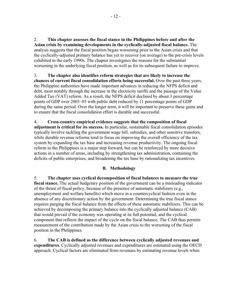
2. This chapter assesses the fiscal stance in the Philippines before and after the Asian crisis by examining developments in the cyclically-adjusted fiscal balance. The analysis suggests that the fiscal position began worsening prior to the Asian crisis and that the cyclically-adjusted primary balance has yet to recover (on average) to the pre-crisis levels exhibited in the early 1990s. The chapter investigates the reasons for the substantial worsening in the underlying fiscal position, as well as for its subsequent failure to improve.

3. The chapter also identifies reform strategies that are likely to increase the chances of current fiscal consolidation efforts being successful. Over the past three years, the Philippine authorities have made important advances in reducing the NFPS deficit and debt, most notably through the increase in the electricity tariffs and the passage of the Value Added Tax (VAT) reform. As a result, the NFPS deficit declined by about 3 percentage points of GDP over 2003–05 with public debt reduced by 11 percentage points of GDP during the same period. Over the longer term, it will be important to preserve these gains and to ensure that the fiscal consolidation effort is durable and successful.

4. Cross-country empirical evidence suggests that the composition of fiscal adjustment is critical for its success. In particular, sustainable fiscal consolidation episodes typically involve tackling the government wage bill, subsidies, and other sensitive transfers, while durable revenue reforms tend to focus on improving the overall efficiency of the tax system by expanding the tax base and increasing revenue productivity. The ongoing fiscal reform in the Philippines is a major step forward, but can be reinforced by more decisive actions in a number of areas, including by strengthening tax administration, containing the deficits of public enterprises, and broadening the tax base by rationalizing tax incentives.

B. Methodology

5. The chapter uses cyclical decomposition of fiscal balances to measure the true fiscal stance. The actual budgetary position of the government can be a misleading indicator of the thrust of fiscal policy, because of the presence of automatic stabilizers (e.g., unemployment and welfare benefits) which move in a countercyclical fashion even in the absence of any discretionary action by the government. Determining the true fiscal stance requires purging the fiscal balance from the effects of these automatic stabilizers. This can be achieved by decomposing the primary balance into the cyclically adjusted balance (CAB) that would prevail if the economy was operating at its full potential, and the cyclical component that reflects the impact of the cycle on the fiscal balance. The CAB thus permits measurement of the contribution made by the Asian crisis to the worsening of the fiscal position in the Philippines.

6. The CAB is defined as the difference between cyclically adjusted revenues and expenditures. Cyclically adjusted revenues and expenditures are estimated using the OECD approach. Cyclical factors are eliminated from revenues by estimating revenue levels when

- 13 -

output is at its potential, assuming average elasticity for the period 1990–2004.10 It is assumed that given limited welfare benefits and in the absence of unemployment benefits in the Philippines, expenditure is largely independent of cyclical developments and therefore cyclically adjusted expenditures are equal to actual expenditures.11

7. The fiscal stance is then defined as the first difference in the CAB.12 The fiscal stance can be a useful measure of the impact of fiscal policy on aggregate demand and can be employed to determine whether the fiscal policy is procyclical or counter-cyclical. A positive correlation between the fiscal stance and the output gap in a particular period indicates that fiscal policy was procyclical during that period.

8. Procyclicality of fiscal policy may have important implications for macroeconomic stability and fiscal sustainability. A recent IMF study concludes that procyclical fiscal policy exacerbates economic fluctuations, with adverse consequences for savings, investment, economic growth, and welfare. It also suggests that a stronger procyclical bias in the upturn may result in a deteriorating fiscal position over time, since deficits and debt built up during bad times are in general not offset during good times.13

C. Findings

9. Analysis of the CAB indicates that the deterioration in the underlying fiscal position predates the Asian crisis. Developments in cyclically-adjusted revenues and expenditures suggest that fiscal policy was loosened from 1995, prior to the Asian crisis (Figure 2). Cyclically-adjusted revenues fell, despite the tax reforms undertaken in the early and mid-1990s (Box 1), while primary spending increased substantially. Fiscal policy was also procyclical during the crisis.

10. The decline in the cyclically adjusted revenues prior to crisis can be attributed to a number of factors. Although the fiscal reforms helped to substantially boost tax receipts in the first half of the 1990s, the increase in revenues may have fallen short of potential because a number of structural weaknesses were not addressed. In particular, the reforms failed to

10 Potential output is calculated by de-trending time-series data of real GDP, using the Hodrick-Prescott (HP) filter. Sensitivity analysis shows that the results are generally robust with respect to elasticity assumptions.

11 The formula used to calculate the CAB in year t is: CABt=Rt(Ypt/Yt)α -Et, where R is actual revenue;

Yp is potential output; Y is actual output; α is the average elasticity of revenue with respect to Yp/Y for the period 1990–2004; and E is the actual expenditure.

12 A negative number implies a reduction in the CAB.

13 For further details on causes and consequences of procyclicality in fiscal policy see FAD 2005.

- 14 -

rein in extensive tax incentives and did not tackle weaknesses in tax administration.14 In addition, the operating receipts of the Government Owned and Controlled Corporations (GOCCs) declined following the privatization in 1994 of the oil refining and distribution company Petron—a subsidiary of the Philippine National Oil Company (PNOC).

Figure 2. The Philippines: Cyclically Adjusted Balance and Output Gaps, 1990-2004(In percent of GDP)

Source: Philippine authorities; and Fund staff estimates.

Actual and Cyclically Adjusted Primary Balance

-1

0

1

2

3

4

5

6

7

8

1990 1992 1994 1996 1998 2000 2002 2004

Interest

Primary balance

Cyclically adjusted primary balance

Cyclically Adjusted Revenues and Expenditures

15

20

25

30

1990 1992 1994 1996 1998 2000 2002 2004

CA Revenue

CA Primary Expenditure

Revenue

Output Gap and Fiscal Stance

-7

-5

-3

-1

1

3

5

7

1991 1993 1995 1997 1999 2001 2003

Output gapFiscal stance

Output Gap and Fiscal Stance

-6.0

-4.0

-2.0

0.0

2.0

4.0

6.0

-4.0 -3.0 -2.0 -1.0 0.0 1.0 2.0 3.0 4.0

Output gap (in percent of potential GDP)

Fiscal stance

11. Spending policy was stimulative on average in the first half of the 1990s, including in the years immediately preceding the crisis, when output was above potential. Budget allocations favored increases in statutory outlays—including government wages and transfers to the local governments—over spending on infrastructure and maintenance. Primary expenditure expanded by almost 2 percentage points of GDP during 1995–97, with personnel outlays increasing by over 1½ percentage points of GDP.

14 For the discussion of the drawbacks of the fiscal reforms undertaken in the early and mid-1990s, see Kostial and Summers (1999).

- 15 -

Box 1. Philippines: National Government Tax Revenue Developments in 1990–2004

Two distinct periods can be identified in the Philippines’ tax revenue performance over the period 1990–2004. Prior to the Asian crisis, tax revenues increased strongly, likely as a result of tax reforms undertaken in the late 1980s and mid-1990s. Following the crisis, however, tax revenues fell off sharply and have not yet recovered to their pre-crisis levels.

Despite the on-going trade liberalization, the NG tax ratio increased by almost 3 percentage points of GDP during 1990–97. Over two-thirds of the increase can be attributed to buoyant income tax collection, in particularly on corporate profits, and the remaining third to higher VAT receipts possibly on account of the expanding tax base. The on-going trade liberalization offset some of these gains, resulting in a loss of over ½ percent of GDP in the annual tax ratio over the eight-year period. The tax ratio peaked at 17 percent of GDP in 1997.

Various tax reforms may have played a role in strengthening the revenue collection. The first reform was started under the Aquino administration in 1986 and included the introduction of the VAT in 1988, which replaced a multi-rate manufacturers’ tax, and changes in individual and corporate income tax. This reform was followed by the expansion of the VAT in 1994 to include services that were previously subject to percentage taxes and the introduction of a Comprehensive Tax Reform package (CTRP) in 1997. Under the CTRP, ad valorem taxes on tobacco products and alcoholic beverages were replaced with specific excises; and the taxation of petroleum products was revamped by a substantial reduction in import tariffs and the introduction of petroleum excises.

However, the revenue gains from these reforms were not sustained. National government tax revenues declined by over 4½ percentage points of GDP between 1997 and 2004. About one-third of the decline came as a result of the continuing trade liberalization and another third from lower excises that were not indexed to inflation. The remainder of the decline can be attributed to lower income tax collection (1 percent of GDP) and weaker indirect taxes, including the VAT (0.5 percent of GDP). The factors contributing to the decline in the tax ratio since the crisis are discussed in the text.

The Philippines: Composition of Tax Revenues, 1990-2004 (In percent of GDP)

0.0

2.0

4.0

6.0

8.0

10.0

12.0

14.0

16.0

18.0

1990 1991 1992 1993 1994 1995 1996 1997 1998 1999 2000 2001 2002 2003 2004

OtherDutiesVATExcisesIncome

- 16 -

12. These revenue and expenditure trends persisted after the Asian crisis. From 1998 onward, cyclically-adjusted revenues generally follow the unadjusted revenue trend, reflecting relatively small cyclical fluctuations during 1999–2004 (Figure 1). After a brief improvement in 1998, cyclically-adjusted revenues continued on a declining path, closely tracking the sharp fall in national government (NG) tax collections. NFPS revenues were also affected by a decline in GOCC receipts which fell by 1½ percentage points of GDP between 1998 and 2004. Some of this decline came as a result of a moderation in the demand for electricity following the Asian crisis and unfavorable contracts between the National Power Corporation (NPC) and independent power producers (IPPs).15 However, the primary factor explaining the deterioration in NPC’s revenues was the government’s decision in 2002 to cap increases in electricity tariffs and a number of subsequent pro-consumer tariff decisions.16 Statutory expenditure outlays peaked at 15.4 percent of GDP in 2003, after increasing by 2.3 percentage points compared to the 1990 level. The share of statutory outlays in total NG expenditure went up by over 14 percentage points to 79 percent in 2003. This marked change in expenditure composition led to a less flexible budget, which has limited discretionary expenditure policy over the past few years to cuts in capital and maintenance spending (Figure 4).

13. There could be several explanations for why the underlying fiscal position did not improve following the Asian crisis. First, as described above, fiscal policy was procyclical before and during the crisis and the stimulative expenditure policy continued into the early-2000s.17 Second, the revenue reforms that boosted NG tax revenues enjoyed only temporary success for the following reasons: (i) while the VAT tax base was expanded, important sectors, including energy, were left out of the base; (ii) the income tax base was eroded by a proliferation of tax incentives in rapidly expanding sectors of the economy,

15 See also Manasan (2004) for an analysis of GOCC financial performance since the Asian crisis. 16 For more information on the causes behind the weak financial performance of NPC see Box 3 in IMF (2004). 17 Fiscal policy was on average procyclical during 1990-2004, with output gaps positively correlated with the fiscal stance in 9 out of 14 years.

Figure 3. The Philippines: National Government Tax Revenue and Statutory Outlays, 1990-2004

(Percent of GDP)

12

13

14

15

16

17

18

1990 1991 1992 1993 1994 1995 1996 1997 1998 1999 2000 2001 2002 2003 2004

Tax revenue

Statutory outlays

- 17 -

including electronics;18 (iii) the revenues lost from trade liberalization were not replaced; and (iv) specific excises were not indexed to inflation. Third, tax administration weaknesses persisted and were not addressed.19 And finally, the weak financial position of public enterprises, including the state power company (NPC), contributed to the decline in the NFPS revenues.

18 For a description of tax incentives in the Philippines, see Chalk (2001).

19 For an analysis of revenue trends in the Philippines since the Asian crisis, see Inchauste (2002).

Source: The Philippine authorities; and Fund staff estimates.

1990

Personnel, 29.0

Maintanence, 14.1

LGU transfers, 3.4

Capital spending, 14.3

Other, 6.0

Interest, 33.2

Figure 4. The Philippines: NG Expenditure Composition(In percent of total expenditure; unless stated otherwise)

2003

Personnel, 33.0

Maintanence, 9.4LGU

transfers, 17.3

Capital spending, 9.6

Other, 1.8

Interest , 28.9

The Philippines: NG Primary Expenditure Composition, 1990-2004 (Percent of GDP)

0

2

4

6

8

10

12

14

16

18

1990 1991 1992 1993 1994 1995 1996 1997 1998 1999 2000 2001 2002 2003 2004

Personnel Maintanence LGU transfers Capital spending Other

- 18 -

D. Making Fiscal Consolidation a Success

14. Since taking office in mid-2004, the administration has made important progress in addressing the fiscal problem. To this end, the government has launched a comprehensive fiscal reform program. The cornerstone of this program and the measure with the highest revenue potential is the VAT reform that extends the VAT base to energy products and allows for an increase in the VAT rate from 10 to 12 percent in early 2006. The authorities plan to spend a portion of the revenue proceeds from the VAT reform on funding priority infrastructure projects and boosting social spending.

15. Other measures will support the fiscal consolidation. Excise taxes on alcohol and tobacco products were increased by 30 percent on average at end-2004, although not fully indexed to inflation. The authorities are also actively pursuing a government rationalization program that should make the civil service leaner and more effective and improve government service delivery. Finally, significant progress has been made in containing the deficits of public enterprises, including by increasing electricity tariffs—a measure that has more than halved NPC’s deficit.

16. Considerable fiscal gains have already been achieved following the introduction of these reforms, but it will be important to lock in and build up on these gains. In this regard, findings from the recent literature on the link between the composition of fiscal adjustment and its sustainability can be used to identify possible strategies for making the ongoing fiscal consolidation effort a long-lasting success.

17. Recent empirical research finds that the composition of fiscal adjustment is crucial for its sustainability. In particular, sustainable fiscal consolidation episodes typically involve cutting unproductive expenditures, while durable revenue reforms tend to focus on broadening the tax base and increasing revenue productivity. Studies of fiscal adjustment episodes in OECD countries found that fiscal consolidations based on tax increases and cuts in capital spending tend to be shorter-lived than those that rely primarily on reducing outlays on transfers and the wage bill (Alesina and Perotti, 1995 and 1997). A more recent study of emerging market economies suggests that, in addition to cuts in wasteful spending, durable revenue mobilization and robust capital spending are also important components of a sustainable fiscal consolidation (Gupta, et al., 2003).

18. A simple intuitive explanation can be offered to support these results. Spending cuts in politically sensitive expenditure categories, such as wages, pensions, and subsidies, require strong political will and public backing, signaling a sound commitment to fiscal consolidation in countries that managed to successfully carry out these reforms. Similarly, durable reforms on the revenue side, such as introducing new taxes and expanding the base of existing taxes, usually require legislative amendments that are more difficult to reverse than administrative or executive orders, resulting in a longer lasting fiscal consolidation. In contrast, procyclical fiscal policies that encourage exuberant spending in good times may make it difficult to undo the deficits and debt built up during economic downturns.

- 19 -

19. The ongoing fiscal reforms in the Philippines are broadly in line with these findings. The reformed VAT bill should widen the revenue base by including previously exempt energy products and professional services in the tax net. The authorities are also attaching high priority to increasing productive spending on infrastructure, while reducing unproductive expenditure, including through civil service reform. Effective and timely implementation of these reforms is therefore key to the success of fiscal consolidation. However, to enhance the quality of fiscal consolidation and ensure its durability, these efforts would need to be supplemented by other high-quality reforms. These include:

• Enhancing the revenue system by broadening the tax base, including through a meaningful rationalization of income tax incentives. While the VAT reform marks an important advance in this area, international comparison suggests that there is much upside potential to improving revenue performance in the Philippines (Box 2).

• Ensuring that past revenue gains are not eroded over time, including by indexing excises to inflation and revising the level of excises in line with revenue needs and other public policy objectives.

• Strengthening tax administration, including through improved taxpayer registration, audit strategies, return processing, and debt collection techniques.

• Ensuring long-term sustainability of the pension system by conducting regular actuarial reviews and adjusting benefits and contributions in line with the long-term solvency of the system.

• Rebalancing the composition of public spending away from statutory outlays to ensure adequate financing of infrastructure and maintenance spending. In this regard, the government’s decision to spend a share of the incremental revenue from the reformed VAT on infrastructure is a step in the right direction.

20. The deficits of the GOCCs also need to be contained to ensure that all subsectors of the public sector contribute to the adjustment effort. The recent progress made in reducing the large deficit of NPC will need to be solidified by ensuring full cost recovery and delivering successful privatization of the power sector over the medium term. Since high unchecked deficits of the GOCCs may undermine the NFPS fiscal consolidation strategy, it will be important to develop and enforce medium-term deficit targets for the GOCCs that would be aligned with the fiscal targets for the public sector as a whole.

21. Procyclical fiscal policies should be avoided, whenever feasible. Such policies may unfortunately become inevitable during economic downturns due to the need to preserve the sustainability of public finances—especially in countries like the Philippines that face serious vulnerabilities stemming from the high debt burden and large gross financing requirement. In addition, sharp spending increases in good times can exacerbate economic volatility and damage fiscal sustainability over the longer run and therefore should be avoided. In this regard, the cautious spending stance in recent years bodes well for making the adjustment more durable, although expenditure composition can be improved, as discussed above.

- 20 -

Box 2. Philippines: International Comparison of Revenues and Expenditures

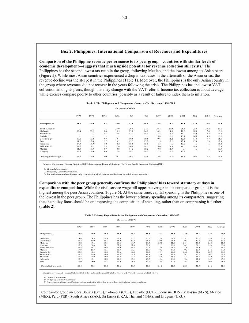
Comparison of the Philippine revenue performance to its peer group—countries with similar levels of economic development—suggests that much upside potential for revenue collection still exists.1 The Philippines has the second lowest tax ratio in the group, following Mexico, and the lowest among its Asian peers (Figure 5). While most Asian countries experienced a drop in tax ratios in the aftermath of the Asian crisis, the revenue decline was the steepest in the Philippines (Table 1). Moreover, the Philippines is the only Asian country in the group where revenues did not recover in the years following the crisis. The Philippines has the lowest VAT collection among its peers, though this may change with the VAT reform. Income tax collection is about average, while excises compare poorly to other countries, possibly as a result of failure to index them to inflation.

1993 1994 1995 1996 1997 1998 1999 2000 2001 2002 2003 Average

Philippines 2/ 15.6 16.0 16.3 16.9 17.0 15.6 14.5 13.7 13.5 12.5 12.5 14.9

South Africa 1/ ... ... ... 25.0 26.0 27.0 26.7 26.0 26.3 25.8 26.2 26.1Malaysia 19.4 20.1 19.6 19.5 19.8 16.8 14.2 14.3 18.8 18.8 17.6 18.1Thailand 1/ ... ... 17.5 17.8 17.1 15.3 14.4 14.5 14.9 15.6 16.7 16.0Bolivia 1/ ... ... ... ... ... ... 15.8 16.1 15.4 16.8 16.5 16.1Colombia 2/ 10.8 10.0 9.7 10.1 10.8 10.6 10.6 11.2 13.3 11.9 13.7 11.1Peru 11.6 12.4 12.7 13.1 13.3 13.2 12.5 12.2 12.4 12.0 12.9 12.6Indonesia 14.4 15.9 15.0 14.2 16.0 15.0 16.3 ... 13.2 ... ... 15.0Sri Lanka 2/ 17.5 17.2 17.8 17.0 16.0 14.5 15.0 14.5 14.6 14.0 ... 15.8Mexico 11.3 10.7 10.7 10.8 11.2 10.2 10.8 11.7 ... ... ... 10.9Uruguay 19.4 19.0 16.9 17.4 18.5 19.3 17.5 16.7 17.5 ... ... 18.0

Unweighted average 3/ 14.9 15.0 15.0 16.1 16.5 15.8 15.4 15.2 16.3 16.4 17.3 14.5

Sources: Government Finance Statistics (IMF); International Financial Statistics (IMF); and World Economic Outlook (IMF).

1/ General Government. 2/ Budgetary Central Government. 3/ For each revenue classification, only countries for which data are available are included in the calculation.

(In percent of GDP)

Table 1. The Philippines and Comparator Countries Tax Revenues, 1990-2003

Comparison with the peer group generally confirms the Philippines’ bias toward statutory outlays in expenditure composition. While the civil service wage bill appears average in the comparator group, it is the highest among the peer Asian countries (Figure 6). At the same time, capital spending in the Philippines is one of the lowest in the peer group. The Philippines has the lowest primary spending among its comparators, suggesting that the policy focus should be on improving the composition of spending, rather than on compressing it further (Table 2).

1993 1994 1995 1996 1997 1998 1999 2000 2001 2002 2003 Average

Philippines 2/ 13.8 13.9 14.4 15.0 16.1 15.4 16.1 15.3 14.9 15.1 14.1 14.9

Bolivia 1/ 24.6 24.3 22.9 23.3 25.2 27.7 27.4 27.1 29.3 30.7 29.6 26.5Colombia 2/ 21.3 22.0 25.1 28.0 27.3 28.0 29.9 28.3 29.3 30.3 29.5 27.2Malaysia 19.8 19.6 19.1 19.6 18.7 19.3 20.0 21.1 26.4 26.0 26.1 21.4Uruguay 27.3 29.0 29.1 27.5 27.8 29.0 31.5 30.0 30.9 29.1 25.6 28.8South Africa 1/ 25.8 25.1 24.6 24.0 23.2 22.6 22.0 21.2 21.6 21.9 23.3 23.2Mexico 19.8 20.7 18.1 18.7 19.5 18.6 18.3 19.0 19.3 20.4 21.1 19.4Ecuador 2/ 22.2 18.4 19.8 20.6 19.4 20.5 19.1 19.9 20.0 21.6 20.7 20.2Sri Lanka 2/ 21.2 20.6 23.6 21.3 19.5 19.5 18.6 19.9 19.7 17.2 16.2 19.8Thailand 1/ 16.5 16.0 15.0 17.4 19.3 17.8 16.9 16.1 16.4 16.3 15.6 16.7Indonesia 13.7 13.1 11.8 11.5 15.1 13.7 13.4 18.0 15.4 12.8 14.9 13.9Peru 12.4 14.0 15.2 15.0 14.8 15.2 15.9 15.7 15.2 14.7 14.8 14.8

Unweighted average 3/ 20.4 20.3 20.4 20.6 20.9 21.1 21.2 21.5 22.1 21.9 21.6 21.1

Sources: Government Finance Statistics (IMF); International Financial Statistics (IMF); and World Economic Outlook (IMF).

1/ General Government. 2/ Budgetary Central Government. 3/ For each expenditure classification, only countries for which data are available are included in the calculation.

Table 2. Primary Expenditure in the Philippines and Comparator Countries, 1990-2003

(In percent of GDP)

1 Comparator group includes Bolivia (BOL), Colombia (COL), Ecuador (ECU), Indonesia (IDN), Malaysia (MYS), Mexico (MEX), Peru (PER), South Africa (ZAR), Sri Lanka (LKA), Thailand (THA), and Uruguay (URU).

- 21 -

22. A durable fiscal adjustment supported by high-quality measures can bring important benefits in the form of higher investment and growth. Empirical research, including recent studies by the IMF, shows that growth and unemployment respond more favorably to longer lasting, better-quality, fiscal adjustment.20 Fiscal reforms perceived as durable lend credibility to government policies and signal that the adjustment effort is sustainable, thereby boosting market confidence and increasing private investment.

23. Sustainable fiscal consolidation in the Philippines can bring a number of tangible benefits. It would create a more stable and favorable investment environment, attracting higher private capital inflows. Moreover, lower deficits would reduce risk premia and interest payments creating room in the budget for productive expenditure, including on infrastructure, while smaller statutory outlays would improve the ability of fiscal policy to react to economic cycle.

20 For a review of the existing literature on expansionary fiscal contractions, see Hemming et al. (2002).

- 22 -

Figure 5. Tax Revenues in the Philippines and Comparator Countries 1/(In percent of GDP)

Sources: Government Finance Statistics (IMF); International Financial Statistics (IMF); and World Economic Outlook (IMF). 1/ 2003 or latest available year. Data may differ from other tables and charts presented in this paper due to the difference in sources used. VAT data for the Philippines do not include taxes collected at the border.

Tax revenue

0

5

10

15

20

25

30

ZAR MYS URU THA BOL LKA COL IDN PER PHL MEX0

5

10

15

20

25

30

Income taxes

0

2

4

6

8

10

12

14

16

ZAR

MY

S

COL

IDN

PHL

THA

MEX PE

R

URU

LKA

BOL

0

2

4

6

8

10

12

14

16VAT

0.0

1.0

2.0

3.0

4.0

5.0

6.0

7.0

PER

BOL

URU

LKA

ZAR

COL

IDN

THA

MEX

MY

S

PHL

0

1

2

3

4

5

6

7

Excises

0

1

2

3

4

5

THA

BOL

URU

LKA

ZAR

PER

MY

S

PHL

MEX ID

N

COL

0

1

2

3

4

5 Taxes on International Trade

0.0

0.5

1.0

1.5

2.0

2.5

3.0

PHL

LKA

THA

MY

S

PER

COL

BOL

URU ID

N

MEX ZA

R

0.0

0.5

1.0

1.5

2.0

2.5

3.0

- 23 -

Figure 6. Expenditures in the Philippines and Comparator Countries 1/(In percent of GDP)

Primary spending

0

5

10

15

20

25

30

35

BOL COL MYS URU ZAR MEX ECU LKA THA IDN PER PHL0

5

10

15

20

25

30

35

Wages and salaries

0

2

4

6

8

10

12

ZAR BOL MEX COL ECU PHL URU THA MYS PER LKA IDN0

2

4

6

8

10

12

Capital spending

0

2

4

6

8

10

12

MYS BOL COL IDN ECU LKA MEX THA PHL URU PER ZAR0

2

4

6

8

10

12

Sources: Government Finance Statistics (IMF); International Financial Statistics (IMF); World Economic Outlook (IMF); CEIC Database; EMED Database and FAD databases (IMF)1/ 2003 or latest available year. Data may differ from other tables and charts presented in this paper due to the difference in data sources.

- 24 -

References

Alesina, A. and Roberto Perotti, 1997, “Fiscal Adjustment in OECD Countries: Composition and Macroeconomic Effects,” IMF Staff Papers, Vol. 44, No. 2 (June), pp. 210–48.

Alesina, A. and Roberto Perotti, 1995, “Fiscal Expansion and Fiscal Adjustments in OECD Countries,” Economic Policy, Vol. 21, pp. 205–48.

Chalk, N., 2001, “Tax Incentives in the Philippines: A Regional Perspective,” Working Paper WP/01/181, International Monetary Fund, Washington D.C.

Fiscal Affairs Department (FAD), 2005, “Cyclicality of Fiscal Policy and Cyclically Adjusted Fiscal Balances,” International Monetary Fund, Washington D.C.

Gupta, S, et al. 2003, “What Sustains Fiscal Consolidations in Emerging Market Countries?” Working Paper WP/03/224, Selected Issues SW/02/266, International Monetary Fund, Washington D.C.

Heller, P. et al, 1986 “A Review of the Fiscal Impulse Measure,” Occasional Paper 44, International Monetary Fund, Washington D.C.

Hemming, R, Michael Kell, and Selma Mahfouz, 2002, “The Effectiveness of Fiscal Policy in Simulating Economic Activity—A Review of the Literature,” Working Paper WP/02/208, International Monetary Fund, Washington D.C.

Honjo, K., 2001, “Cyclically Adjusted Fiscal Balance in Uruguay,” Chapter II in Uruguay, IMF Country Report No. 01/47, International Monetary Fund, Washington D.C.

Inchauste, G. 2002, “Issues in Fiscal Sustainability,” Chapter III in Philippines—Selected Issues SW/02/266, International Monetary Fund, Washington D.C.

IMF Country Report No. 04/317, 2004, Philippines: 2004 Post Program Monitoring Discussions Staff Report, International Monetary Fund, Washington D.C.

Kostial, K. and Victoria Summers, 1999, “Public Finance: Sustainable Fiscal Adjustment,” Chapter III in Philippines—Selected Issues SW/99/149, International Monetary Fund, Washington D.C.

Manasan, R., 2004, “The Philippines’ Fiscal Position: Looking at the Complete Picture,” Philippine Institute for Development Studies Policy Note No. 2004-07.

Ramirez Rigo, E. 2005, “Sustainability of the Fiscal Adjustment” in Moghadam, R. et al. 2005, “Turkey at the Crossroads: From Crisis Resolution to EU Accession,” Occasional Paper 242, International Monetary Fund, Washington D.C.

- 25 -

III. EXPLAINING ECONOMIC GROWTH IN THE PHILIPPINES21

A. Introduction

1. To boost the performance of the economy, the Philippines has embarked on a comprehensive reform program since mid-2004. In the immediate aftermath of World War II, the Philippines had one of the highest per capita GDP in the East Asia region. However, the country’s growth performance has since been disappointing with per capita GDP slipping behind fast-growing East Asia economies (such as Korea, Malaysia, and Thailand) by 2003. The reform program, which is detailed in the Medium-Term Philippine Development Plan (MTPDP), covers a broad reform agenda including economic policy, infrastructure, and institutions. This chapter discusses the Philippines’ growth performance over the past few decades, and then examines the extent to which this can be explained using determinants suggested by recent growth theory.

B. Philippines’ Growth Performance

2. The Philippines has struggled to raise economic growth much above population growth over the past 30 years. With GDP growth lower and population growth higher, per capita GDP growth has lagged behind other developing economies, particularly fast-growing East Asia economies (Table 1). During the 1980s, the Philippines experienced a deep political and debt crisis which led to a large contraction in per capita GDP over the decade (Figure 1). In response, the authorities implemented major economic reforms, resulting in a more outward-oriented and liberalized economic system with less government intervention. In the 1990s, per capita growth rates picked up, but remain lower than other developing economies.22

21 Prepared by Kotaro Ishi (kishi@imf.org).

22 For a comprehensive discussion about the Philippines’ growth performance, see Balisacan and Hill (2003).

Table 1. GDP and Population Growth, 1970-2003 1/(Annual percent change )

GDP PopulationGDP per

capita

Philippines 3.6 2.5 1.1

Developing economies 2/ 4.3 2.1 2.2Selected East Asia 6.5 1.7 4.8

Indonesia 5.8 1.9 3.9Korea 7.3 1.3 6.0Malaysia 6.7 2.5 4.1Thailand 6.3 1.7 4.5

Industrial economies 2.9 0.7 2.2

World 3/ 3.8 1.1 2.6

Source: IMF, World Economic Outlook; and World Bank, WorldDevelopment Indicators.

1/ Regional data are averaged with purchasing power parity GDP weights. 2/ Excludes China.3/ Includes China.

Figure 1. Real Per Capita GDP Growth(Average annual growth; in percent) 1/

-1

0

1

2

3

4

5

6

7

1970s 1980s 1990s 2000-03

PhilippinesSelected East Asia 2/Other Developing Economies 3/

Sources: IMF, World Economic Outlook; and World Bank, World Development Indicators.1/ Regional data are averaged with purchasing power parity GDP weights.2/ Indonesia, Korea, Malaysia, and Thailand.3/ Excludes China.

- 26 -

Figure 2. Philippines: GDP per capita(Constant 2000 U.S. dollars)

700

750

800

850

900

950

1,000

1,050

1,100

1970 74 78 82 86 90 94 98 02

Source: World Bank, World Development Indicators.

3. The Philippines’ growth pattern has been uneven (Figure 2). This is partly due to the country’s large vulnerability to external shocks, such as terms of trade shocks in the 1970s, global interest rate hikes in the early 1980s, power crises in 1992–93, as well as adverse political and natural shocks, including several coup attempts, the volcanic eruption of Mount Pinatubo (in 1991), and droughts caused by El Niño (particularly after 1998).

4. The sources of growth in the Philippines can be decomposed using standard growth accounting. The production process (Y) is assumed to be conventional Cobb-Douglas technology, which utilizes physical capital (K) and labor (L) as inputs, as well as total factor productivity (A):

( ) αα −=

1ttttt LhKAY

where α represents the elasticity of output with respect to physical capital, t is the year, and h is the human capital stock per worker. Expressing all variables in per worker terms (denoted by small caps) and taking log derivatives with respect to time, yields (omitting time indices),

hh

kk

AA

yy &&&&

)1( αα −++=

where xx /& represents growth of a variable x. Growth in output per worker can be decomposed into that due to changes in total factor productivity, physical capital per worker, and human capital per worker. Note that total factor productivity is measured as a residual, and a change in measured productivity might reflect not only technological innovation but also political and external shocks, changes in government policies and institutions, and a measurement error.23

5. Growth accounting results suggest that the low growth in the Philippines is largely attributable to stagnant capital formation and low total factor productivity.24 Physical capital in the Philippines grew at a slower pace than other developing economies in the 1980s and 1990s, while total factor productivity growth was negative or zero (Table 2). However, more recently, output per worker has increased, driven by a significant 23 Other shortcomings of growth accounting include the need to make a fairly arbitrary assumption about the production function form. There is an extensive discussion on growth accounting issues in Bosworth and Collins (2003).

24 Except for the Philippines, data are due to Bosworth and Collins (2003). The Philippine data are staff calculations.

- 27 -

Table 2. Growth Accounting 1/(Annual percent changes)

Contributions to output per worker growthTFP

Output per worker

Physical capital per

workerHuman Capital

With human capital

adjustment

Without human capital

adjustment

1980-89 average

Philippines -0.5 0.3 0.8 -1.6 -0.9Developing economies 0.3 0.5 1.6 -1.8 -0.2

East Asia 2/ 3.9 2.4 1.8 -0.2 1.5Industrial economies 1.4 0.6 0.6 0.3 0.8All economies 0.6 0.5 1.3 -1.2 0.1

1990-99 average

Philippines 0.4 0.3 0.7 -0.7 0.0Developing economies 1.0 0.4 1.1 -0.5 0.6

East Asia 3.4 2.6 1.0 -0.2 0.8Industrial economies 1.5 0.6 0.5 0.5 0.9All economies 1.1 0.5 0.9 -0.2 0.7

2000-04 average

Philippines 1.7 0.4 0.6 0.7 1.3

Sources: Bosworth and Collins (2003); and Fund staff calculations.

1/ Regional averages are simple average.2/ Indonesia, Korea, Malaysia, and Thailand.

-5

-4

-3

-2

-1

0

1

2

3

4

5

1976 1979 1982 1985 1988 1991 1994 1997 2000 2003

ServicesIndsutryAgricultureTotal

Figure 3. Philippines: Labor Productivity (GDP/Employment) Growth

(5-year backward average; contributions; in percent)

Sources: Fund staff calculations. See Annex 2.

improvement in total factor productivity growth. Behind this improvement is a rise in productivity of the services sector, possibly reflecting the rapidly expanding telecommunications industry (Figure 3).

C. Explaining Growth in the Philippines

6. Philippines’ growth performance can be analyzed in terms of potential growth determinants. Much of the recent growth literature (see Rodrik, Subramanian, and Trebbi, 2002 and Rodrik, 2003) emphasizes the role of geography, economic policies, and institutions as determinants of growth.25 How the Philippines fares compared to other regional economies is examined in terms of each of these factors:

Geography

7. Geography sets a country’s advantages and disadvantages due to its physical location. Bloom, Sachs, Collier, and Udry (1998), Gallup, Sachs, and Mellinger (1999), and Sachs (2001) argued that geography influences growth through various channels. For example, geography would shape a large part of natural resource endowments, soil quality, and climate, which determine availability of marketable natural resources (such as oil), land productivity, and the public health environment. Geography is also an important determinant of trade and inward foreign direct investment from advanced economies, since a distant or landlocked country faces greater costs of transport.

25 The demographic profile of the Philippines may also have had an effect on growth performance. However, the empirical support for such an effect is inconclusive (see Kongsamut and Vamvakidis, 2003) and demographic variables are not included in this study.

- 28 -

8. For the Philippines, geography does not appear to be a disadvantage. Table 3 compares the Philippines with other economies in terms of major geographical indicators selected from Gallup et al (1999).26 The Philippines is in an advantageous position in transport with all population having access to the sea, high population density in coastal regions, and shorter distance to world markets. However, the Philippines has a tropical climate and a relatively high malaria index.

Economic policies

9. Positive correlations between policy reforms such as increasing trade openness and growth have been widely documented, as have the negative links between high inflation and growth. The Philippines has undertaken increasingly outward-oriented and market-based policies since the mid-1980s, including trade liberalization, privatization of government assets, strengthening of central bank independence, opening of sectors to foreign direct investment, and liberalization of domestic shipping, oil, and telecommunications. Kongsamut and Vamvakidis (2000) find that these policy shifts contributed to better economic performance in the Philippines in the 1990s.

10. These policies have been maintained to varying degrees in recent years (Figure 4). Since the 1990s, average inflation in the Philippines has declined, while the Philippines has also experienced a substantial increase in trade openness. However, the size of the fiscal deficit and external debt (in percent of GDP) in the Philippines has increased, much more so than in other East Asia economies. The size of government has also increased, while the total investment share to GDP has declined to the lowest in the sample period. After a significant improvement in the 1990s, net foreign direct investment (FDI) inflows 26 Gallup, et al (1999) concluded that (i) tropical regions are hindered in development relative to temperate regions; (ii) coastal regions, and regions linked to coasts by ocean-navigable waterways, are strongly favored in development relative to the hinterlands; (iii) landlocked economies may be particularly disadvantaged by their lack of access to the sea; (iv) high population density in coastal regions would be favorable for growth, as evidenced by the fact that high growth in developing economies has often been achieved through labor intensive manufacturing exports that require good access to internal and international trade; (v) greater transport costs (measured in distance from core capital-goods-supplying regions, such as the U.S., Western Europe, and Japan) and the prevalence of infectious diseases are negatively correlated with growth.

Table 3. Geography

Philippines East Asia 1/All developing

economies

Indicators related to integrationProportion of the region’s population within 100 km of the coastline or ocean-navigable river 1.0 0.8 0.5

Density of human settlement (population per km2) in the coastal region (within 100 km of the coastline) 230.3 215.0 144.6

Density of human settlement (population per km2) in the interior (beyond 100 km from the coastline) 56.0 78.6 69.3Landlocked (Yes=1, No=0) 0.0 0.0 0.2Average distance by air of the economies within the region to the closest “core” capital-goods-supplying regions, such as the U.S., Western Europe, and Japan (in km) 3,010.0 4,237.5 5,050.0

Indicators related to natural resources and climateProportion of land area within the geographical tropics 1.0 0.8 0.7Index of Malaria prevalence (from 0, low, to 1, high) 0.6 0.3 0.4

Source: Gallup, Sachs, and Mellinger (1999).

1/ The simple average of Indonesia, Korea, Malaysia, and Thailand.

- 29 -

Figure 4. Economic Policy Indicators 1/(Period average)

1. Indicators generally improved over the past 30 years

2. Indicators generally worsened or remained poorer than other East Asia economies

Inflation(In percent)

0

4

8

12

16

20

1970s 1980s 1990s 2000-Present

Philippines

East Asia

Trade Openness(Sum of exports and imports, in percent of GDP)

0

20

40

60

80

100

120

140

1970s 1980s 1990s 2000-Present

Philippines

East Asia

Fiscal Deficit(General government, in percent of GDP)

-2

0

2

4

6

1970s 1980s 1990s 2000-Present

Philippines

East Asia

External Debt(In percent of GDP)

0

20

40

60

80

100

1970s 1980s 1990s 2000-Present

Philippines

East Asia

have declined in recent years, as has privatization activity, although it should be noted that this has also declined in other East Asia economies. Public infrastructure quality in the Philippines has improved over the last decade, but remains below the East Asia average.

- 30 -

Figure 4. Economic Policy Indicators (continued)(Period average)

Sources: International Monetary Fund, World Economic Outlook database and International Financial Statistics; World Bank, WorldDevelopment Indicators and Privatization database.1/ East Asia is the simple average of Indonesia, Korea, Malaysia, and Thailand. 2/ Composite index of the quality of telephone, roads, irrigated land, electricity, and water. With a higher index number indicating betterinfrastructure. See Annex 2 for details.

Government Size(General government consumption, in percent of

GDP)

5

7

9

11

13

15

1970s 1980s 1990s 2000-Present

Philippines East Asia

Total Investment(In percent of GDP)

10

15

20

25

30

35

40

1970s 1980s 1990s 2000-Present

Philippines East Asia

Net FDI(In percent of GDP)

0.0

0.4

0.8

1.2

1.6

2.0

1970s 1980s 1990s 2000-Present

PhilippinesEast Asia

Public Infrastructure 2/(Index ranging from 0 to 100)

0

10

20

30

40

50

60

70

1970s 1980s 1990s 2000-Present

Philippines East Asia

Privatization(Privatization value, in percent of GDP)

0

2

4

6

8

10

12

14

16

1990s 2000-Present

Indonesia

Malaysia

Philippines

Thailand

- 31 -

Figure 5. Governance Indicators 1/(2000-04 average)

-0.8 -0.6 -0.4 -0.2 0.0 0.2 0.4 0.6 0.8

Voice andaccountability

Governmenteffectiveness

Regulatory quality

Rule of law

Control ofcorruption

DevelopingeconomiesEast Asia 2/

Philippines

Source: Kaufmann, et al (2005).1/ The indicators are measured in units ranging from about -2.5 to 2.5, with higher values corresponding to better governance outcomes.2/ The simple average of Indonesia, Korea, Malaysia, and Thailand.

Institutions

11. The recent growth literature emphasizes the role that institutions play. In general, “good” institutions are considered to contribute to growth through two channels.27 First, the quality of institutions affects the investment climate, and hence long-run growth (Hall and Jones, 1999; Acemoglu, Johnson, and Robinson, 2000). Second, good institutions strengthen the government’s ability to adjust policies to exogenous shocks (Rodrik, 1999).

12. Drawing from the recent literature, this chapter focuses on the following three measures of institutions: first, the quality of governance, including government effectiveness, regulatory quality, and rule of law; second, the effectiveness of the legal system and property rights; and third, political stability (see Annex 2 for details of the data).

• The quality of governance matters for overall economic development as it determines government effectiveness and efficiency in utilizing or allocating public resources.28 According to governance indicators, produced by Kaufmann, Kraay, and Masutruzzi (2005), the Philippines ranks poorly compared to the average developing and East Asia economies on all indicators but “voice and accountability”(Figure 5). In particular, “control of corruption,” and “rule of law” indicators are ranked much lower in the Philippines than in the other economies.

• Legal system and property rights affect the incentives to invest and innovate as investors are concerned about the protection of their investment returns.29 Legal system and property rights indicators, produced by the Cato Institute (2004), show that the Philippines fares worse than other economies in most components of the indicators (Figure 6).

• Political stability is key to assure investors of the continuity of economic policies. According to “political risk index” provided by International Country Risk Guide

27 North (1990), who is widely cited in the literature, defined institutions as the set of formal rules and informal conventions that provide the framework for human interaction and shape the incentives of members of society. See International Monetary Fund, World Economic Outlook (2003 and 2005) for more discussion about the role of institutions.

28 See Kaufmann, Kraay, and Zoido-Lobaton (1999), Philippine Senate Economic Planning Office (2004), and World Bank (2005).

29 See Accemoglu, Johnson, and Robinson (2001) and Dollar and Kraay (2002).

- 32 -

Figure 6. Legal System and Property rights Indicators (2003) 1/

0 2 4 6 8 10

Judiciaryindependence

Impartial courts

Protection ofintellectual property

Military in politics

Law and order

DevelopingeconomiesEast Asia 2/

Philippines

Source: The Cato Institute.1/ The indicators are measured in units ranging from 0 to 10, with higher values corresponding to better outcomes.2/ The simple average of Indonesia, Korea, Malaysia, and Thailand.

(ICRG), the Philippines scores worse than Malaysia and Thailand, but better than Indonesia and the average for developing economies (Figure 7). Similarly, Gurr, Jaggers, and Marshall’s indicator on “constraints on executives” shows that the Philippines ranks slightly above the average developing economy.30

D. Growth Regressions

13. Standard cross-country regression analysis is employed to examine the relative importance and validity of these explanatory factors. The following two questions are considered: first, how important are geographic factors in explaining the Philippines’ long-run growth record; and second, how much of the Philippines’ growth performance (total factor productivity and capital accumulation growth) can be explained by other factors, such as economic policy and institutions.

14. The first exercise investigates the importance of geography on growth, using cross-section regressions. In a sample of 79 advanced and developing economies, the model regresses the log level of per capita GDP in 2003 or the average annual growth rate of per capita GDP over the period 1965–2003 on geography variables. A Philippine dummy variable is included in each regression to examine whether the Philippines is unusual compared to the average across sample economies.

30 A society in which elites and politicians are effectively constrained is expected to experience less infighting between various groups to take control of the state, and to pursue more sustainable policies.

Figure 7. Political Risk and Constraints on Executives 1/

40

45

50

55

60

65

70

75

Philippines Indonesia Malaysia Thailand Developingeconomies

0

1

2

3

4

5

6

7

Political risk (LHS)

Constraints on executives(RHS)

Sources: ICRG and Gurr, et al.1/ The political risk is measured in units ranging from 0 to 100, with higher values corresponding to lower risk; while constraints on executives is measured from 1 to 7, with higher values corresponding to more constraints (lower political risk).

- 33 -

Figure 8. Per Capita GDP Level: Actual vs. Prediction 1/

2

3

4

5

2 3 4 5

Actual per capita GDP in 2003 (log)

Pred

icte

d pe

r ca

pita

GD

P (l

og)

PhilippinesThailand

MalaysiaKorea

1/ Based on the regression result Table A1 (1) without the Philippine dummy.

Figure 9. Per Capita GDP Growth: Actual vs. Prediction 1/

-2

0

2

4

6

8

-2 0 2 4 6 8

Actual per capita GDP growth (percent)

Pred

icte

d pe

r ca

pita

GD

P gr

owth

(per

cent

) Philippines

Malaysia

Thailand

Korea

1/ Based on the regression result Table A1 (2) without the Philippine dummy.

15. The estimation results confirm the close relationship between geography and economic development. As reported in Table A1, the level of per capita GDP or growth rates of per capita GDP is a positive function of the population density in coastal regions (Population 100km), and a negative function of tropical regions (Tropical area), transport costs (LDistance), and malaria prevalence (Malaria index in 1966 or 1994). The Philippines’ dummy is not significant, suggesting that the Philippines’ growth performance is just what one would expect for a country with the Philippines’ geographical conditions. This result contrasts with other Asian economies where both predicted levels and growth rates of per capita GDP are lower than actual levels, implying that those economies perform better than they would given their geography (Figure 8 and 9). More formally, in the per capita GDP growth regression, Korea, Malaysia, or Thailand dummies are found to be highly significant.31

16. The second exercise looks at correlations of growth with economic policy and institution variables. A sample of 81 advanced and developing economies is used to examine which explanatory variables are most strongly correlated with GDP per worker, physical capital per worker, or total factor productivity. Observations are averaged for three 10-year periods over 1970–99, thereby excluding cyclical components of GDP. The model is estimated by ordinary least squares (OLS) with a Philippines dummy, as well as feasible generalized least squares with random effects. 32, 33

31 T statistics for Korea, Malaysia, and Thailand are 3.17 (p value, 0.01), 2.50 (0.03), 3.62 (0.00), respectively. In the GDP per capita level regression, dummy variables are not found to be significant.

32 As extensively discussed in other studies, economic policy and institution variables may be considered endogenous. However, it is not easy to find effective instruments for each endogenous variable (see for example, Bosworth and Collins, 2003). Hence, regression results without controlling endogeneity problem are presented, which are interpreted to show correlation and not causality.

33 Random effects model is chosen, rather than fixed effects model, because the fixed effects model discards time-invariant country specific factors, which in the current case, are geography variables.

(continued)

- 34 -

Figure 10. GDP per Worker Growth: Actual vs. Prediction (1990-99 average) 1/

-4

-2

0

2

4

6

-8 -4 0 4 8 12

Actual GDP per worker growth (percent)

Pred

icte

d G

DP

per

wor

ker

grow

th(p

erce

nt)

Philippines

Thailand

Malaysia

1/ Based on the regression result Table A2 (3) without the Philippine dummy.

Korea

17. The final results, reported in Table A2, suggest that:

• Consistent with the results of the previous cross-section regressions, geography variables, particularly Tropical area, are significantly correlated with GDP per worker growth (model 1), although the significance of these variables reduces or disappears if economic policy and institution variables are added (models 2–8).

• Most of the economic policy variables have the expected sign and are significant in the GDP per worker equations, although government fiscal balance becomes insignificant if institution variables are added (models 3 and 4). Economic policy variables appear to affect total factor productivity (models 5 and 6) more significantly than capital accumulation (models 7 and 8).

• The institution variable is highly correlated with GDP per worker growth (models 3 and 4). It is also noteworthy that the variable appears to be more significant in capital accumulation equations (models 7 and 8) than in total factor productivity equations (models 5 and 6), suggesting that institutions are of particular importance for capital accumulation.

• Philippine dummy variables are insignificant, implying that the Philippines’ growth performance is just the average of the sample economies conditional on the set of explanatory variables (Figure 10).

• Growth performance in Korea, Malaysia, and Thailand can also be well explained by these regressions: none of the dummy variables for these economies are significant. This appears to suggest that over-performance of East Asia economies, which were not explained by the previous cross-section geography regressions, can be attributed to their better economic policy and institutions.

E. Conclusions

18. The main finding in this chapter is that the Philippines’ growth performance is well explained by geography, economic policies, and institutions. The empirical results support the authorities’ reform priorities in MTPDP. In particular, more sustainable fiscal

The Hausman tests are employed to test the validity of the random effects, which proves inconclusive, because the result differs across models.

- 35 -

policy, an improvement in infrastructure quality as well as institutions—that is to say a better investment climate—could significantly raise the Philippines’ growth potential.

19. The regression results permit a rough simulation of the benefits of reform. Although the regression results represent simple correlations (not causality), the predicted increase in growth on account of an improvement in explanatory factors can be calculated as an illustration (Table 4). For example, an improvement in “law and order” by about one rating (from 3.3 to 4.5, the average of Malaysia and Thailand) would be associated with a 0.3 percentage points increase in long-run growth of GDP per worker. These results underscore the likely importance of sound economic policy and better institutions for the long run economic development of the Philippines.

GDP per Of which: 2/ worker growth TFP growth Capital per worker

Improvement in "law and order" by one rating 0.3 0.2 0.1Improvement in infrastructure to the level of the East Asia average 3/ 0.8 0.5 0.3

Reduction of external debts by 10 percentage points of GDP 0.4 0.2 0.2

1/ Based on estimated parameters in Table A2 (4), (6), and (8).2/ Contributions to GDP per worker growth. 3/ Korea, Indonesia, Malaysia, and Thailand.

Table 4. What are Predicted Increases in Growth Rates? 1/ (Percentage points change)

- 36 - ANNEX I

The Regression Exercise The first regression exercise: cross section regressions on growth and geography. The following cross section equation is estimated by ordinary least squares (OLS) using the data of a sample of 79 advanced and developing economies.

iii GDPcapitaperinitialY ][βµ += iii dummysPhilippineiablesgeography εϕγ +++ ][]var[ , where i denotes an economy and ),(~ 2

ii oIID σε .

The dependent variables, Yi, are the logarithm of per capita GDP in U.S. dollars in 2003 or the average annual growth rates of per capita GDP over the period 1965–2003. Initial levels of per capita GDP are included for the per capita growth regression to capture catching-up effects. A set of geography variables are due to Gallup, et al. (1999) (see Annex 2 for details of data). A Philippine dummy variable (for the Philippines, value 1, otherwise, 0) is included to examine if the Philippines is unusual compared to the average across sample economies. The estimation results are:

Table A1. Cross Section Regression 1/

Dependent variablePer capita GDP

in 2003Per capita GDP growth over

1965-2003(1) (2) (3)

Constant 5.63 4.25 5.27( 14.73 ) *** (2.28) ** (2.80) ***

Per capita GDP in 1965 ... -0.52 -0.54(-1.49) (-1.58)

Tropical area -0.40 -1.11 ...(-3.08) *** (-2.66) ***

Population 100 km 0.37 1.41 0.87( 2.68 ) *** (-3.38) *** (2.00) **

LDistance -0.57 -0.39 -0.64(-4.97) *** (-0.97) (-1.73) *

Malaria index 1994 -0.70 ... ...(-4.65) ***

Malaria index 1966 ... ... -1.37(-2.98) ***

Philippine dummy -0.22 -0.80 -0.80(-0.57) (-0.61) (-0.62)

No. of observations 79 79 79Adjusted R-squared 0.77 0.21 0.23

Source: Fund staff estimates.1/ T-statistics in parenthesis (***, **, and * indicate significant at 1, 5 and 10percent, respectively).

- 37 - ANNEX I

The second regression exercise: panel regressions on growth and economic policies and institutions. The following panel equation is estimated by OLS or random effects model to take account of country-specific random factors. In a sample of 81 advanced and developing economies, the data are averaged for three 10-year periods over 1970–99.

itiit iablesexogenousY ]var[βµ += itiablespolicyeconomic ]var[δ+ itiablesninstitutio ]var[γ+

iti εα ++ ,

where i and t denote an economy and time, respectively; ),(~ 2ασα oIIDi and ),(~ 2

εσε oIIDit .

Dependent variables, Yit, are the average growth rates of GDP per worker, total factor productivity, or physical capital per worker. Explanatory variables can be categorized into three: exogenous variables, such as Tropical area, Population 100km (both measures of geography), initial per capita GDP, and terms of trade volatility (a measure of external shock); economic policy variables such as inflation, government balance, openness, external debt, and infrastructure; and institution variables such as ICRG law and order, political risk, and Economic Freedom’s legal system and property rights (see Annex 2 for details of data).34 We start with a broad range of potential explanatory variables and drop those that prove clearly insignificant. A Philippine dummy variable (for the Philippines, value 1, otherwise, 0) is included in the OLS models to examine if the Philippines is unusual compared to the average across sample economies. The estimation results are:

34 These institutions variables are chosen due to availability of time series data. However, even these variables lack the first period 1970–79, for which the same data for the second period 1980–89 are used. Furthermore, due to high correlations, only one institution variable was included in each regression. Although not reported, other institution variables, such as “Economic Freedom’s legal system and property rights” and “ICRG political risk” were found to be highly significant.

- 38 - ANNEX I

Table A2. Panel Regression 1/

Dependent variable GDP per worker growth TFP growth 2/ Capital per worker growthOLS OLS OLS Random OLS Random OLS Random

(1) (2) (3) (4) (5) (6) (7) (8)

Constant 5.40 7.19 7.06 7.01 4.06 4.03 8.59 8.51( 6.36 ) *** ( 8.86 ) *** ( 8.77 ) *** ( 8.57 ) *** ( 5.99 ) ( 6.09 ) ( 7.36 ) *** ( 6.95 )

Initial per capita GDP 2/ -1.14 -1.87 -2.15 -2.22 -1.23 -1.23 -2.63 -2.63(-4.68) *** (-7.94) *** (-8.23) *** (-8.48) *** (-5.60) *** (-5.71) *** (-6.94) *** (-6.84) ***

Tropical area -2.09 -1.06 -0.89 -0.97 -0.67 -0.68 -0.63 -0.88(-6.16) *** (-3.35) *** (-2.77) *** (-2.85) *** (-2.47) ** (-2.58) *** (-1.35) (-1.61)

Population 100km 1.03 0.07 0.15 0.19 -0.23 -0.26 1.09 1.28( 2.76 ) *** ( 0.21 ) ( 0.48 ) ( 0.56 ) (-0.84) (-0.99) ( 2.36 ) ** ( 2.27 ) **

Terms of trade ... -0.03 -0.03 -0.02 -0.03 -0.03 0.0004 0.013(-2.99) *** (-2.19) ** (-1.57) (-2.61) *** (-2.61) *** ( 0.02 ) ( 0.72 )

Inflation -0.001 -0.001 -0.001 -0.001 -0.001 -0.001 -0.001(-1.99) ** (-1.85) * (-1.71) * (-1.66) * (-1.68) * (-0.88) (-0.84)

Government balance ... 0.06 0.04 0.04 0.04 0.04 0.003 -0.02( 2.43 ) ** ( 1.68 ) ( 1.62 ) ( 1.95 ) * ( 1.93 ) * ( 0.09 ) (-0.45)

Openness ... 0.01 0.01 0.006 0.004 0.004 0.004 0.003( 4.30 ) *** ( 3.82 ) *** ( 3.68 ) *** ( 3.35 ) *** ( 3.48 ) *** ( 1.97 ) ** ( 1.38 )

External debt ... -0.37 -0.39 -0.37 -0.16 -0.16 -0.66 -0.61(-6.03) *** (-6.39) *** (-6.15) *** (-3.10) *** (-3.20) *** (-7.46) *** (-7.15) ***

Infrastructure ... 3.82 3.70 3.69 2.26 2.23 4.09 3.69( 4.05 ) *** ( 3.95 ) *** ( 3.87 ) *** ( 2.88 ) *** ( 2.91 ) *** ( 3.02 ) *** ( 2.60 ) ***

ICRG law and order ... ... 0.24 0.29 0.14 0.15 0.29 0.30( 2.37 ) ** ( 2.76 ) *** ( 1.61 ) ( 1.75 ) * ( 1.99 ) ** ( 1.86 ) *

Philippine dummy -0.83 -1.22 -1.00 ... -0.67 ... -0.94 ...(-0.70) (-1.26) (-1.03) (-0.82) (-0.67)

No. of observations 243 243 243 243 243 243 243 243Adjusted R-squared 0.14 0.42 0.43 0.42 0.32 0.28 0.35 0.34Sample periods 1970-1999

Source: Fund staff estimates

1/ The data set comprises 10-year average of each variable. T-statistics are in parenthesis (***, **, and * indicate significant at 1, 5and 10 percent, respectively).2/ Without human capital adjustments. The main thrust of the results hold even for TFP growth with human capital adjustments.

- 39 - ANNEX II

Data used for the Regression Exercise Per capita GDP in1965 (or 2003): The logarithm of per capita GDP in U.S. dollars in 1965 (or 2003). Sources: International Monetary Fund, World Economic Outlook (WEO); and World Bank, World Development Indicators (WDI). Per capita GDP growth over 1965–2003: The average annual growth rate (percent) of GDP per capita over the period 1965–2003. Sources: WEO; and WDI. Tropical area: The proportion of the country’s land area within the geographical tropics. Data are calculated by Gallup, et al. (1999) using ArcWorld Supplement database. See http://www.cid.harvard.edu/ciddata/ciddata.html. Population 100 km: The proportion of the population in 1994 within 100 km of the coastline. Data are calculated by Gallup, et al. (1999) using the GIS population dataset. See http://www.cid.harvard.edu/ciddata/ciddata.html. LDistance: The logarithm of the minimum Great-Circle (air) distance in kilometers to one of the three capital-goods-supplying regions: the U.S., Western Europe, and Japan, specifically measured as distance from the country’s capital city to New York, Rotterdam, or Tokyo. Data are calculated by Gallup, et al. (1999). See http://www.cid.harvard.edu/ciddata/ciddata.html. Malaria index in 1966 (or 1994): Index of malaria prevalence based on a global map of extent of malaria in 1966 and the fraction of falciparum malaria in 1966 (or 1994). Data are calculated by Gallup, et al. (1999) using World Health Organization database. The variable has a scale from 0 to 1, with a higher score indicating greater malaria prevalence. See http://www.cid.harvard.edu/ciddata/ciddata.html. Data used mainly in second (panel) regression exercise GDP per worker: Real GDP per worker in local currencies. For non-Philippine economies, calculated by Bosworth and Collins (2003) using WDI and OECD Statistical Compendium. For the Philippines, calculated by staff using WDI, CEIC, and International Labor Organization, Labor Statistics Database. Human capital quality (used for the growth accounts): Average years of education of population 15 and older. Data are calculated by Bosworth and Collins using Barro and Lee (2000) and Cohen and Soto (2001). Capital stock (used for the growth accounts): Estimated using a perpetual inventory model, where the depreciation rate equals 0.05. For non-Philippine economies, calculated by Bosworth and Collins, using Nehru and Dhareshwar (1993). For the Philippines, calculated by staff using the Philippine National Accounts.

- 40 - ANNEX II

Initial per capita GDP: Logarithms of GDP per capita in constant U.S. dollars in 1970, 1980, and 1990. Source: WDI. Terms of Trade (volatility): Standard deviations of annual growth rate of terms of trade. Source: WDI. Inflation: Average annual inflation of CPI. Sources: International Monetary Fund, International Financial Statistics and WEO; and WDI. Government balance: Government fiscal balance as a percent of GDP. Government is either national or general government depending on the data availability. Source: WEO. Openness: The sum of exports of goods and services and imports of goods and services divided by GDP. Source: WDI. External debt: Data in Figure 4 are gross external debt. Data used in the panel regressions are net external debt, transformed to an index raging from 1 (low) to 8 (high), with "1" indicating net external debt GDP ratio below 40 percent and "8" above 100 percent. Sources: WDI and Lane and Milesi-Ferretti (forthcoming). Infrastructure: Simple average of fixed line and mobile phone subscribers (per 100 people), paved roads (percent of total roads), irrigated land (percent of cropland), 100 minus electric power transmission and distribution losses (percent of output), and improved sanitation facilities (percent of population with access). Source: WDI. ICRG law and order: A measure of the strength and impartiality of the legal system and the popular observance of the law. The variable has a scale from zero to six, with a higher score indicating better legal system and rule of law. Source: International Country Risk Guidance (ICRG). See http://www.icrgonline.com/. ICRG political risk: A measure of assessing the political stability of a country by assessing risk factors including government stability, socioeconomic conditions, investment profile, internal conflict, external conflict, corruption, military in politics, religious tensions, law and order, ethnic tensions, democratic accountability, and bureaucracy quality. The variable has a scale from 0 to 100, with a higher score indicating lower risk. Source: ICRG. See http://www.icrgonline.com/. Other data used in tables and figures. Kaufmann, Kraay, and Masutruzzi (2005)’s governance indicators: • Control of corruption: Absence of use of public power for private gain or corruption.

• Rule of law: the protection of persons and property against violence or theft, independent and effective judges, contract enforcement.

- 41 - ANNEX II

• Regulatory burden: the relative absence of government controls on goods markets, banking system, and international trade.

• Government effectiveness: the quality of public service delivery and competence of the civil service, including the degree of its politicization.

• Voice and accountability: the extent to which citizens can choose their government, political rights, civil liberties, and independent press.

For more details, see http://www.worldbank.org/wbi/governance/govdata/.

The Cato Institute (2004)’s economic freedom indicators:

• Law and order: Data are from ICRG.

• Military in politics: Military interference in rule of law and the political process. Data are from ICRG.

• Protection of intellectual property: Data are from World Economic Forum, Global Competitiveness Reports (GCR).

• Impartial courts: A trusted legal framework exists for private businesses to challenge the legality of government actions or regulation. Data are from GCR.

• Judicial independence: the judiciary is independent and not subject to interference by the government or parties in disputes. Data are from GCR.

For the regression analysis, a composite index of these variables is used. For more details, see http://www.cato.org/pubs/efw/.

Gurr, Jaggers, and Marshall’s Polity IV Project database

• Constraints on executives: Operational (de facto) independence of chief executive of a state. The variable has a scale from 1 to 7, with a higher score indicating more constraints.

For more details, see http://www.cidcm.umd.edu/inscr/polity/.

- 42 -

References

Acemoglu, Daron, Simon Johnson, and James A. Robinson, 2001, “The Colonial Origins of Comparative Development: An Empirical Investigation.” American Economic Review, Vol. 91.

Balisacan, Arsenio M., and Hal Hill (edit), 2003, The Philippine Economy: Development,

Policies, and Challenges, Ateneo De Manila University Press. Barro, Robert J., and Jong-Wha Lee, 2000, “International Data on Educational Attainment,

Updates and Implications”, National Bureau of Economic Research, Working Paper, No. 7911.

Bloom, David E., Jeffrey D. Sachs, Paul Collier, and Christopher Udry, 1998, “Geography,

Demography, and Economic Growth in Africa,” Brookings Papers on Economic Activity, Vol. 1998, No. 2.

Bosworth, Barry P. and Susan M. Collins, 2003, “The Empirics of Growth: An Update,”

Brookings Papers on Economic Activity, Vol. 2003, No. 2. Cohen, Daniel, and Marcelo Soto, 2001, “Growth and Human Capital: Good Data, Good

Results,” OECD Technical Paper 179, September. Dollar, David, and Aart Kraay, 2002, “Institutions, Trade, and Growth,” Journal of Monetary

Economics, Vol. 50, No. 1. Gallup, John Luke, Jeffery D. Sacks, and Andrew Mellinger, 1999, “Geography and

Economic Development,” Center for International Development at Harvard University Working Paper No. 1, March.

Gwartney, James, Robert Lawson, and Erik Gartzke, 2004, “Economic Freedom of the

World: 2005 Annual Report,” The Cato Institute. Hall, Robert E., and Charles I. Jones, 1999, “Why Do Some Countries Produce So Much

More Output per Worker than Others?” The Quarterly Journal of Economics, Vol. 114, No. 1.

International Monetary Fund, 2003, “World Economic Outlook,” 2003 September. _______________________, 2005, “World Economic Outlook,” 2005 September. Lane, Philip R., and Gian Maria Milesi-Ferretti (forthcoming), “The External Wealth of

Nations Mark II: Revised and Extended Estimates of Foreign Assets and Liabilities, 1970–2004,” International Monetary Fund Working Paper.

- 43 -

Kaufmann, Daniel, Aart Kraay, and Pablo Zoido-Lobaton (1999), “Governance Matters,” World Bank Policy Research Department Working Paper, No. 2196.

Kaufmann, Daniel, Aart Kraay, and Massimo Mastruzzi (2005), “Governance Matters IV:

Governance Indicators for 1996–2004,” World Bank Policy Research Working Paper Series No. 3630, May.

Kongsamut, Piyabha, and Athanasios Vamvakidis, 2003, “Philippines: Toward Sustainable

and Rapid Growth—Recent Developments and the Agenda Ahead,” International Monetary fund, Occasional Paper 187.

Nehru, Vikram, and Ashok Dhareshwar, 1993, “A New Database on Physical Capital Stock:

Sources, Methodology, and Results,” Revista de Anălisis Econŏomico 8(1): 37–59. North, Douglass G., 1990, Institutions, Institutional Change, and Economic Performance

(Cambridge University Press). Philippine Senate Economic Planning Office, 2004, “Five Pillars of Economic Growth: An

Economic and Social Development Framework.” Rodrik, Dani, 1999, “Where Did All the Growth Go? External Shocks, Social Conflict, and

Growth Collapses,” Journal of Economic Growth, Vol. 4, No. 4. Rodrik, Dani, 2003, “What Do We Learn From Country Narratives,” Chapter 1, In Search of

Prosperity, ed. by Dani Rodrik (Princeton University Press). Rodrik, Dani, Arvind Subramanian, and Francesco Trebbi, 2002, “Institutions Rule: The

Primacy of Institutions over Geography and Integration in Economic Development,” National Bureau of Economic Research, Working Paper, No. 9305.

Sachs, Jeffrey D., 2001, “Tropical Underdevelopment,” National Bureau of Economic

Research, Working Paper, No. 8119. World Bank, 2005, “The Philippines towards a Better Investment Climate for Growth and

Productivity,” a paper presented at workshop on “Policies to Strengthen Productivity in the Philippines” on June 27, 2005.

- 44 -

IV. SECOND-ROUND EFFECTS OF THE OIL SHOCK ON INFLATION35

A. Introduction

1. Since early-2004, a series of supply shocks has increased inflation above target in the Philippines and threatened to drive inflation expectations higher. Foremost among these shocks has been the surge in international oil prices, which rose 41 percent in 2005, after rising 31 percent in 2004 and 16 percent in 2003. In responding to these shocks, the Bangko Sentral ng Pilipinas (BSP) has followed the standard inflation targeting approach, namely, accommodating immediate effects on the price level, but increasing policy rates on indications of a possible rise in expectations of inflation. While the BSP has been able to strike a balance—repeated tightening over the past year has helped put inflation on a downward trajectory—it is in practice often difficult to distinguish the immediate impact of supply side shocks on inflation from a more fundamental shift in medium-term inflation expectations. This distinction is especially hard to make in the Philippines, where a series of supply side shocks has pushed inflation substantially above target in both 2004 and 2005. 2. This chapter assesses the impact of the recent surge in international oil prices on medium-term inflation expectations in the Philippines. Conceptually, the impact of an oil shock on inflation can be thought of as consisting of first-, second-, and third-round effects. First-round effects consist of (i) direct pass through from international oil prices to domestic fuel prices, where the speed of this channel depends on whether there are fuel subsidies and on the competitive structure of the energy sector; and (ii) indirect effects which capture the role of fuel products as intermediate inputs in production. Second-round effects occur when the first-round rise in inflation “spills over” into perceptions of medium-term inflation, as households and firms adjust their price and wage setting behavior. Third-round effects can arise from a country being a net importer of oil, so that a rise in oil prices reduces domestic incomes and spending. In addition, higher oil prices may also lower growth in key trading partners. Lower activity may in turn reduce medium-term inflation pressures.36 3. To assess the impact of the oil shock on inflation expectations, this chapter uses core inflation to capture the second-round effects of the recent surge in oil prices. Since survey data on inflation expectations in the Philippines are limited, a proxy for second-round effects is needed. Measures of core inflation are an obvious candidate, as they aim to strip out the first-round effects of supply shocks. However, there exist many different ways to measure core inflation, so this chapter first reviews a widely-used list of core inflation measures and compares their ability to predict changes in headline inflation. It then uses the

35 Prepared by Robin Brooks (rbrooks2@imf.org).

36 This classification draws on the September 2005 Monetary Policy Statement of the Reserve Bank of New Zealand.

- 45 -

Figure 1: Headline Inflation(Jan. 2003 - Dec. 2005, in percent)

-2

0

2

4

6

8

10

12

14

16

2003M1 2003M7 2004M1 2004M7 2005M1 2005M7

m/m (annualized, sa)

y/y

Inflation Trend

Episode 1: rise in food price inflation(trend inflation 6.5 percent)

Episode 2: transport and electricity hikes(trend inflation 9.5 percent)

Epsiode 3: fall in food price inflation(inflation trend 6.4 percent)

Figure 2. Contributions to Headline Inflation(Jan. 2004 - Dec. 2005, annualized m/m, in percent)

-5

0

5

10

15

20

2003M1 2003M7 2004M1 2004M7 2005M1 2005M7

20

25

30

35

40

45

50

55

60Education Services (4%, LHS)Rentals (16%, LHS)Light (4%, LHS)Water (1%, LHS)Land Transport (4%, LHS)Energy (3%, LHS)Food (50%, LHS)Other (19%, LHS)Dubai Oil Price (USD per barrel, RHS)

most successful measure of core inflation to quantify the second-round effects of the recent surge in oil prices on inflation. 4. This chapter is structured as follows. Section B reviews recent inflation developments and identifies a series of supply shocks that have pushed inflation above target in the last two years. Section C introduces some widely-used measures of core inflation and compares them to headline inflation in the Philippines. Section D assesses the relative performance of these measures in predicting changes in headline inflation, while section E uses the most successful measure to quantify second-round effects from the oil shock in the Philippines. As a comparison, similar calculations are performed for Indonesia and Thailand. Section F concludes.

B. Recent Inflation Developments

5. Since 2004, inflation developments in the Philippines can be characterized by three discrete episodes. Figure 1 plots headline inflation in year-on-year (y/y) terms, month-on-month (m/m) terms (annualized, seasonally adjusted), and the inflation trend—the simple mean of m/m inflation over a particular period. The trend measure is a more timely measure of changes in inflation pressures, since y/y inflation is a backward-looking indicator. Figure 1 shows that the recent path of inflation can be broken down into three discrete episodes. Episode 1 saw trend inflation rise from 3.8 percent in 2003 to 6.5 percent from January to May 2004. Episode 2 saw the inflation trend rise still higher, to 9.5 percent from June to December 2004, while Episode 3 encompasses all of 2005, when trend inflation fell back to 6.4 percent, just above the inflation target of 5–6 percent. 6. These episodes can be traced to a series of supply side shocks, the most recent of which is the surge in international oil prices. Food price inflation accelerated sharply in early 2004, as higher cost of animal feed drove meat prices higher. In addition, a shift in demand away from poultry due to the Avian Flu virus pushed fish prices up as well. The rise in international oil prices in 2004 led to fare increases in

- 46 -

Figure 3. One-Year-Ahead Inflation Expectations(Jan. 2002 - Dec. 2005, in percent)

0

1

2

3

4

5

6

7

8

Jan-02 Jul-02 Jan-03 Jul-03 Jan-04 Jul-04 Jan-05 Jul-05

Source: Consensus Economics.

the transport sector in mid-2004. These fare hikes caused the land transport component in the CPI to jump sharply, in part a catch-up effect after being flat for several years. Hikes in electricity tariffs caused the light component in the CPI to jump in late 2004. In 2005, food price inflation moderated as meat imports rose and planting conditions improved, while first-round effects from the surge in oil prices caused the energy component in the CPI to rise sharply towards the end of the year, with knock-on effects on fares in the transport sector. Starting in November, fuel prices began to fall, however, even with implementation of the first stage of the VAT reform law on November 1. As a result, the contribution of energy-related components to CPI inflation was negative in December. Figure 2 shows the contributions to annualized m/m inflation of key CPI items, along with their CPI weights, and the USD price per barrel of Dubai Fateh crude. 7. With the rapid succession of supply side shocks, expectations of inflation one-year-ahead rose in the course of 2004 and have remained high. Figure 3 plots inflation expectations one-year-ahead, using survey data from Consensus Economics. It shows that inflation expectations moved up sharply in the course of 2004 and remained high in 2005. Unfortunately, these data are only available from 2000 and thus do not lend themselves to a systematic exploration of how the oil shock might affect medium-term inflation expectations. In addition, the consensus forecasts tend to lag actual inflation data, so that they may not have much forward-looking content. As a result, this chapter uses core inflation to assess the second-round effects from the surge in oil prices on inflation.37

C. Measures of Core Inflation

8. Measures of core inflation aim to help policy makers identify shifts in medium-term trend inflation. The common rationale underlying all measures of core inflation is to eliminate or discount sharp, quickly reversed movements in prices or one-off shocks that create short-term volatility in headline inflation. Core inflation measures thus tend to be less volatile than headline inflation. There are two basic approaches to constructing core inflation measures. The first, the exclusion-based approach, eliminates certain items from the CPI that are thought to be subject to frequent supply shocks that are in many cases self-reversing. The

37 The BSP’s inflation report, which was first published in Q4 2001, also includes a quarterly survey of private sector inflation forecasts.

- 47 -

official measure of core inflation in the Philippines, which eliminates certain food and energy components in the CPI, falls into this category. A second approach is to eliminate outliers or re-weight the CPI basket according to statistical criteria. These statistics-based measures of core inflation include the trimmed mean, weighted median, both of which are also monitored by the BSP, but there are also many other possible approaches. 9. This chapter constructs five measures of core inflation for the Philippines, all of which exhibit lower volatility than headline inflation. These measures are: • Official measure of core: this exclusion-based measure eliminates rice, corn, fruits and

vegetables, LPG, kerosene, and oil, gasoline and diesel from the CPI basket, with the total weight of excluded CPI items amounting to 18.4 percent in the 2000-based CPI. This measure has the advantage that it is easily communicated to the public, since unlike some of the other measures considered below, the excluded items remain constant over time.

• Trimmed mean: this measure eliminates CPI components with unusually large or small

inflation rates in a given month. The chapter follows the BSP, which measures the trimmed mean as the central 70 percent of the distribution of CPI components, weighted according to their weights in the CPI basket. This measure implicitly assumes that outlying price changes are more likely to reflect relative price changes with no impact on medium-term trend inflation.

• Weighted median: this measure is an extreme case of the trimmed mean, where only the

50th percentile of the weighted distribution of CPI constituent inflation rates is used. The chapter follows the BSP in constructing this measure, where the median inflation rate corresponds to the cumulative CPI weight of 50 percent.

• Persistence-based measure: Blinder (1997) argues that core inflation is the “persistent”

part of inflation that is correlated with future inflation. Cutler (2001) was the first to construct such a measure for the U.K. This chapter constructs a similar measure for the Philippines, estimating an autoregressive (AR) process with 12 lags based on m/m inflation rates for all CPI components and then double weighting CPI constituents according to their weights in the consumption basket and the combined size of the AR estimates, with items with insignificant or negative serial correlation receiving a weight of zero. Items with high persistence include rentals, kerosene, land transport, and oil, gasoline and diesel, while items with low or insignificant persistence include fruits and vegetables, light and water charges.

• Adaptive expectations: Cogley (2002) advocates a measure of core based on adaptive

expectations. Cogley shows that this measure of core is much less volatile than standard measures of core for the U.S. and finds that it outperforms other measures in forecasting changes in headline inflation. This measure is given by:

- 48 -

Mean Standard DeviationHeadline 6.1 4.4Official Core 6.0 3.6Trimmed Mean 4.3 2.9Weighted Median 4.5 3.0Persistence-Based Core 6.6 3.8Adaptive Expectations (g0 = 0.69) 6.1 3.5Adaptive Expectations (g0 = 0.12) 6.5 2.1

Table 1. M/M Inflation in Percent (annualized, sa): Feb. 1994 - Oct. 2005.

where πt

* is core inflation in period t, πt is headline inflation in period t, and g0 is a smoothing parameter that determines the half-life of inflation shocks. Since g0 is an unobserved parameter, it is assumed that the half-life of inflation shocks, based on m/m inflation data (annualized, sa) lies between 1 (g0 = 0.69) and 6 months (g0 = 0.12), where the half-life is given by ln(2)/g0.

Table 1 compares the means and standard deviations for each of these measures of core to headline inflation in the Philippines. It shows that each of these measures exhibits lower volatility than headline inflation, a desirable property for measures of core inflation. However, for some measures the reduction in volatility is larger than for others. At one extreme, the persistence-based measure has a standard deviation of 3.8 percent, while at the other extreme the adaptive expectations measure with g0 = 0.12 has a standard deviation less than half that of headline inflation. In addition, Table 1 shows that some measures of core tend to be biased relative to headline inflation. The trimmed mean and weighted median measures tend to be biased downward, due to the right-skewness of the underlying inflation data, a common problem associated with these measures. Meanwhile, the persistence-based measure and the adaptive expectations measure with g0 = 0.12 are biased upward. 38

D. Choosing Among Measures of Core Inflation

10. The usefulness of a core inflation measure depends on its ability to predict changes in headline inflation. The inflation target in the Philippines is formulated in terms of headline inflation. As such, the primary role of core inflation is to inform policy makers about the future path of headline inflation. To compare how well the various measures of core inflation perform this task, the following equation from Cogley (2002) is estimated: where πt

* represents core and πt stands for headline inflation. This equation assesses whether deviations of headline above core inflation (πt - πt

*) > 0 in period t are on average followed by a deceleration in headline inflation H periods ahead (πt+H – πt). If this is the case, then βH should be negative and significantly different from zero. Indeed, the definition of Bryan and Cecchetti (1994) for core inflation allows one to go further. They define core inflation as “the

38 For a survey of the BSP’s measures of core inflation, see Guinigundo (2004).

( )*10

*1

*−− −+= tttt g ππππ

( ) HtttHHtHt u ++ +−+=− *ππβαππ

- 49 -

Figure 4. Explanatory Power (R2) of Core Inflation Measures(One to thirty-six months ahead)

0%

10%

20%30%

40%

50%

60%

70%80%

90%

100%

1 3 5 7 9 11 13 15 17 19 21 23 25 27 29 31 33 35

Official CoreTrimmed MeanWeighted MedianPersistenceAE (g0 = 0.12)AE (g0 = 0.69)

component of price changes that is expected to persist over medium-run horizons of several years.” In other words, core inflation can be written as πt

* = Etπt+H where H is a suitably long forecast horizon. This means that if core is unbiased relative to headline inflation, then it should be the case that αH = 0 where this restriction follows from the fact that (πt+H – πt) and (πt - πt

*) are (approximately) mean zero. In addition, if πt* = Etπt+H, then it should be the case

that βH = -1, where this restriction measures whether core inflation correctly filters out the transient components in headline inflation. In the regressions below, both parameters are freely estimated and tests are then performed to assess whether the restrictions hold. In order to decide between two measures of core inflation that are similar in terms of αH and βH, the competing measures are also assessed in terms of the R2 in these regressions. Core measures that account for a greater percentage of subsequent changes in inflation filter out more transient variation and are thus preferable to other measures.39 11. The adaptive expectations measure of core outperforms other measures in terms of explaining subsequent variation in headline inflation. For a sample from February 1994 to October 2005, most candidate measures of core tend to exhibit some bias relative to headline as the prediction window lengthens from one to 36 months ahead (αH ≠ 0), while predictive content is relatively good across all measures (βH = -1). The adaptive expectations measure of core with g0 = 0.12 stands out, however, in terms of explaining subsequent variation in headline inflation. Figure 4 shows that the R2 of this measure peaks 24 months ahead at around 60 percent, substantially above any other measure. This suggests that the adaptive expectations measure with g0 = 0.12 does a better job than other measures at filtering out transient components from headline inflation. A technical annex reports αH and βH estimates for the various measures of core inflation.

E. Second-Round Effects from the Oil Shock

12. Second-round effects from rises in international oil prices have historically been large in the Philippines by regional standards. This section estimates a VAR in the ln differences of the USD price per barrel of Dubai Fateh crude, the nominal exchange rate and the adaptive expectations measure of core. This estimation is performed for Indonesia, the Philippines and Thailand for a sample from 1970 Q2 to 2005 Q3 using quarterly data. The smoothing parameter is assumed to be consistent with a half-life for inflation shocks of

39 To ensure that these estimates are robust to a trend decline in inflation, the regressions include a linear time trend.

- 50 -

Headline Core Headline Core Headline CoreQ1 0.33 0.04 -0.17 -0.02 0.10 0.02Q2 0.72 0.14 -0.23 -0.04 0.34 0.07Q3 1.14 0.29 -0.38 -0.08 0.43 0.14Q4 1.34 0.45 -0.23 -0.07 0.60 0.22Q5 1.07 0.56 -0.01 -0.03 0.56 0.29Q6 0.69 0.61 0.29 0.06 0.42 0.32Q7 0.19 0.57 0.65 0.18 0.35 0.33Q8 -0.04 0.50 0.78 0.30 0.27 0.33

Indonesia ThailandTable 2. Additions to y/y Headline and Core Inflation Rates (in ppts).

Philippines

4 quarters (g0 = 0.17), the same value as used by Cogley (2002) for quarterly data. Impulse responses are then generated for a 10 percent permanent shock to the price of Dubai Fateh crude, using this ordering. Table 2 summarizes the results, showing the additions to y/y headline and core inflation rates resulting from this shock. Table 2 shows that the oil shock adds up to 0.6 percentage points to y/y core inflation, substantially above Indonesia and Thailand, in part a reflection of fuel subsidies in the latter two countries, which have only recently been reduced or eliminated. 13. Given the long sample period, it is likely that these estimates for second-round effects are an upper bound for the Philippines. In particular, it is likely that increased competition, greater fiscal discipline and the BSP’s enhanced inflation fighting credentials have in recent years reduced the scope for second round effects. Moreover, the greater pass-through into inflation from changes in international oil prices also points to a strength of the Philippines which has been highlighted recently: the absence of fuel subsidies.

F. Conclusions

14. A 10 percent permanent rise in the price of Dubai Fateh crude is estimated to add up to 0.6 percent to y/y core inflation in the Philippines. This estimate uses the adaptive expectations measure of core to proxy for medium-term inflation expectations, as this measure outperforms other measures in terms of explaining subsequent variation in headline inflation. An added advantage of this measure is that it is easy to construct across countries. Estimated second-round effects are shown to be substantially smaller in Indonesia and Thailand, although these estimates may be biased downward by fuel subsidies, which have only recently been reduced or eliminated. Indeed, going forward, the estimated magnitude of second-round effects for the Philippines is likely an upper bound, as greater competition, ongoing fiscal consolidation and enhanced monetary policy credibility will likely reduce the scope for second-round effects over time.

- 51 - ANNEX I

Technical Annex

Figure A1. Predictive Power of Official Core Measure: βH .(Point estimates bolded, 90 percent confidence interval dotted)

-3.0

-2.5

-2.0

-1.5

-1.0

-0.5

0.0

1 3 5 7 9 11 13 15 17 19 21 23 25 27 29 31 33 35

Figure A2. Predictive Power of Trimmed Mean: βH .(Point estimates bolded, 90 percent confidence interval dotted)

-3.0

-2.5

-2.0

-1.5

-1.0

-0.5

0.0

1 3 5 7 9 11 13 15 17 19 21 23 25 27 29 31 33 35

Figure A3. Predictive Power of Weighted Median: βH .(Point estimates bolded, 90 percent confidence interval dotted)

-3.0

-2.5

-2.0

-1.5

-1.0

-0.5

0.0

1 2 3 4 5 6 7 8 9 10 11 12 13 14 15 16 17 18 19 20 21 22 23 24 25 26 27 28 29 30 31 32 33 34 35 36

Figure A4. Predictive Power of Adaptive Expectations: βH .(Point estimates bolded, 90 percent confidence interval dotted)

-3.0

-2.5

-2.0

-1.5

-1.0

-0.5

0.0

1 3 5 7 9 11 13 15 17 19 21 23 25 27 29 31 33 35

Figure A5. Predictive Power of Persistence Measure: βH .(Point estimates bolded, 90 percent confidence interval dotted)

-3.0

-2.5

-2.0

-1.5

-1.0

-0.5

0.0

1 3 5 7 9 11 13 15 17 19 21 23 25 27 29 31 33 35

Figure A6. Bias of Official Core Measure: αH .(Point estimate bolded, 90 percent confidence interval dotted)

-5

-4

-3

-2

-1

0

1

2

3

4

1 2 3 4 5 6 7 8 9 10 11 12 13 14 15 16 17 18 19 20 21 22 23 24

Figure A7. Bias of Trimmed Mean: αH .(Point estimates bolded, 90 percent confidence interval dotted)

-5

-4

-3

-2

-1

0

1

2

3

4

1 2 3 4 5 6 7 8 9 10 11 12 13 14 15 16 17 18 19 20 21 22 23 24

Figure A8. Bias of Weighted Median: αH .(Point estimates bolded, 90 percent confidence interval dotted)

-4

-3

-2

-1

0

1

2

3

4

1 2 3 4 5 6 7 8 9 10 11 12 13 14 15 16 17 18 19 20 21 22 23 24

Figure A9. Bias of Adaptive Expectations Measure: αH .(Point estimates bolded, 90 percent confidence interval dotted)

-5

-4

-3

-2

-1

0

1

2

3

4

1 2 3 4 5 6 7 8 9 10 11 12 13 14 15 16 17 18 19 20 21 22 23 24

Figure A10. Bias of Persistence-Based Measure: αH .(Point estimates bolded, 90 percent confidence interval dotted)

-5

-4

-3

-2

-1

0

1

2

3

4

1 2 3 4 5 6 7 8 9 10 11 12 13 14 15 16 17 18 19 20 21 22 23 24

- 52 -

References Blinder, A., “Commentary,” Federal Reserve Bank of St Louis Review, May/June 1997. Bryan, M. and S. Cecchetti, “Measuring Core Inflation,” In Monetary Policy, edited by

N. Gregory Mankiw, pp. 195–215, Chicago: University of Chicago Press, 1994. Cogley, T., “A Simple Adaptive Measure of Core Inflation,” Journal of Money, Credit and

Banking, Vol. 34, No. 1 (February 2002), pp. 94–113. Cutler, J., “A New Measure of ‘Core Inflation in the U.K.,’” MPC Unit Discussion Paper

No 3, Bank of England, March 2001.

Guinigundo, D., “An Official Core Inflation Measure for the Philippines,” Bangko Sentral Review, July 2004.

Reserve Bank of New Zealand, “Monetary Policy Statement,” September 2005,

(http://www.rbnz.govt.nz/monpol/statements/sep05.pdf).