PHILIPP KINDT, DANIEL YUNGE, ROBERT DIEMER and SAMARJIT ... · PHILIPP KINDT, DANIEL YUNGE, ROBERT...
46
Precise Energy Modeling for the Bluetooth Low Energy Protocol PHILIPP KINDT, DANIEL YUNGE, ROBERT DIEMER and SAMARJIT CHAKRABORTY, Institute for Real-Time Computer Systems, Technische Universit¨at M¨ unchen March 13, 2014 Abstract Bluetooth Low Energy (BLE) is a wireless protocol well suited for ultra- low-power sensors running on small batteries. It is optimized for low power communication and is not compatible with the original Bluetooth, referred to as Bluetooth Basic Rate (BR)/Enhanced Data Rate (EDR). BLE is described as a new protocol in the official Bluetooth 4.0 specification. It reuses many parts of the Bluetooth BR hardware and software stack to enable dual mode devices supporting Bluetooth BR/EDR and BLE. To design energy-efficient devices, the protocol provides a number of parameters that need to be optimized within an energy, latency and throughput design space. To minimize power consumption, the protocol parameters have to be optimized for a given application. Therefore, an energy-model that can predict the energy consumption of a BLE-based wire- less device for different parameter value settings, is needed. As BLE differs from Bluetooth BR significantly, models for Bluetooth BR cannot be easily applied to the BLE protocol. Since the last one year, there have been a couple of proposals on energy models for BLE. However, none of them can model all the operating modes of the protocol. This paper presents a precise energy model of the BLE protocol, that allows the computation of a device’s power consumption in all possible operating modes. To the best of our knowledge, our proposed model is not only one of the most accurate ones known so far (because it accounts for all protocol parameters), but it is also the only one that models all the operating modes of BLE. Furthermore, we present a sensitivity analysis of the different parameters on the energy consumption and evaluate the accuracy of the model using both discrete event simulation and actual measurements. Based on this model, guidelines for system designers are presented, that help choosing the right parameters for optimizing the energy consumption for a given application. 1 Introduction Optimizing energy consumption is a crucial design requirement in many wireless sen- sor networks. Long battery lifetimes are especially important for body-worn medical sensors, mobile phones and interface devices such as a wireless mouse. To address this issue, recently an ultra-low-power communication protocol, called Bluetooth Low Energy (BLE) has been proposed [13]. BLE-based sensors are able to operate on a coin cell for several months to several years [6], depending on its processing and com- munication demands and the parametrization of the (BLE) protocol. The protocol 1 arXiv:1403.2919v1 [cs.NI] 12 Mar 2014
Transcript of PHILIPP KINDT, DANIEL YUNGE, ROBERT DIEMER and SAMARJIT ... · PHILIPP KINDT, DANIEL YUNGE, ROBERT...
Precise Energy Modeling for the Bluetooth Low
Energy Protocol
PHILIPP KINDT, DANIEL YUNGE, ROBERT DIEMERand SAMARJIT CHAKRABORTY,
Institute for Real-Time Computer Systems, Technische Universitat Munchen
March 13, 2014
Abstract
Bluetooth Low Energy (BLE) is a wireless protocol well suited for ultra-low-power sensors running on small batteries. It is optimized for low powercommunication and is not compatible with the original Bluetooth, referred toas Bluetooth Basic Rate (BR)/Enhanced Data Rate (EDR). BLE is describedas a new protocol in the official Bluetooth 4.0 specification. It reuses many partsof the Bluetooth BR hardware and software stack to enable dual mode devicessupporting Bluetooth BR/EDR and BLE. To design energy-efficient devices, theprotocol provides a number of parameters that need to be optimized within anenergy, latency and throughput design space. To minimize power consumption,the protocol parameters have to be optimized for a given application. Therefore,an energy-model that can predict the energy consumption of a BLE-based wire-less device for different parameter value settings, is needed. As BLE differs fromBluetooth BR significantly, models for Bluetooth BR cannot be easily applied tothe BLE protocol. Since the last one year, there have been a couple of proposalson energy models for BLE. However, none of them can model all the operatingmodes of the protocol. This paper presents a precise energy model of the BLEprotocol, that allows the computation of a device’s power consumption in allpossible operating modes. To the best of our knowledge, our proposed model isnot only one of the most accurate ones known so far (because it accounts for allprotocol parameters), but it is also the only one that models all the operatingmodes of BLE. Furthermore, we present a sensitivity analysis of the differentparameters on the energy consumption and evaluate the accuracy of the modelusing both discrete event simulation and actual measurements. Based on thismodel, guidelines for system designers are presented, that help choosing theright parameters for optimizing the energy consumption for a given application.
1 Introduction
Optimizing energy consumption is a crucial design requirement in many wireless sen-sor networks. Long battery lifetimes are especially important for body-worn medicalsensors, mobile phones and interface devices such as a wireless mouse. To addressthis issue, recently an ultra-low-power communication protocol, called Bluetooth LowEnergy (BLE) has been proposed [13]. BLE-based sensors are able to operate on acoin cell for several months to several years [6], depending on its processing and com-munication demands and the parametrization of the (BLE) protocol. The protocol
1
arX
iv:1
403.
2919
v1 [
cs.N
I] 1
2 M
ar 2
014

2 THE BLE PROTOCOL 2
leaves open a large degree of freedom in terms of choosing the parameter values. Suchparametrizations have a significant impact on the power consumption of the deviceusing the protocol. Along with the power consumption, important aspects of com-munication such as latency and throughput are influenced by this parametrization.For example, the throughput ranges from less than one bit per second (on average)to up to 102kBit/s1, making BLE suitable for a broad range of wireless applications,especially when only small volumes of data have to be transmitted on an average.
As a result, appropriate parameter optimization that takes the application’s re-quirements into account is an important part of the design process. Furthermore,intelligent power management algorithms running on BLE devices can perform onlineparameter optimizations and therefore need to make use of an energy model.
In this paper, we present a precise and comprehensive energy model for BLE inall its possible modes of operation. Our work integrates existing models for BLE andmakes a number of new contributions:
1. Our model takes into account all relevant operating modes and parameters ofthe protocol, whereas all known models till date only capture a limited set ofoperating modes. Towards this, we combine, refine and extend a number ofrecently proposed energy models for BLE.
2. We analyze the variations of parameter values and perform a sensitivity analysisto study their impact on power consumption.
3. We validate the model through detailed experiments, viz., by comparing theresults from our proposed model with those obtained from measurements. Suchcomparisons have not been done for any of the previously proposed energymodels, baring one exception in [8], where only one mode was studied.
The rest of this paper is organized as follows. In Section 2, we give a shortintroduction to the BLE protocol. Related previous work and our contributions aredescribed in Section 3. We then present our proposed energy model for BLE inSection 4. This model is compared against simulations and real world measurementsin Section 5. In Section 6, the model is used to provide guidelines for appropriateparametrization of the protocol in different scenarios. To ease the understanding ofthe equations we present in this paper, a table of symbols is provided in the appendix.
2 The BLE protocol
In this section we give a short overview of the BLE protocol and describe all aspectsof BLE that are important for deriving a power model.
2.1 BLE versus Bluetooth BR/EDR
Originally, Bluetooth was developed as a wireless replacement for cables targetingmobile devices. Most of the data transmitted were pictures, music and video files. Forthese applications, a high speed data link was necessary, which contradicted the goalof extending the lifetime of battery-powered devices. The second type of applicationsinvolved connecting computer peripheral devices such as keyboards and mice to a
1A maximum throughput of approximately 40 kBit/s was reported in [11] and 54.8 kBits/s wasreported in [5] with a CC2540 BLE device. We could measure 102kBit/s on a CC2540-based BLE112device. A derivation in [4] results in a theoretical maximum possible throughput of 236.7 kBit/s.

2 THE BLE PROTOCOL 3
host PC. In this case, the data rate was not a limiting problem, but the batterylifetime had to be extended enormously. To achieve this, the so called Sniff-Mode wasintroduced. For small amounts of data, rather than immediate data transmission,meeting soft deadlines is sufficient. Bluetooth data transmission is organized in timeslices and the Sniff-Mode allows data transmission only in a subset of them. Basedon the volume of data, the slave sleeps and wakes up periodically at the appropriatetime slices. However, in doing so, the master (e.g. a computer) of the Bluetoothconnection is always awake, thereby incurring a high energy consumption.
As mobile devices, especially mobile phones, became more powerful, applicationsusing sensor data became more common and all of them used standard Bluetootheven though it was not designed for this purpose, since the master always needs tobe awake. In addition, standard coin cell batteries that are used in many setupscannot sustain the high peak currents resulting in Bluetooth BR/EDR. To addressthese two issues and achieve higher data rates, Bluetooth evolved in two directions: 1)Bluetooth High Speed (HS) which has a higher data rate for optimized data exchangeand 2) BLE which targets towards small and low cost sensors powered by coin cellbatteries. BLE was developed from its predecessors Wibree and ULP Bluetooth.These were introduced in recognition of the need of an ultra low power wireless datalink in addition to the standard Bluetooth BR/EDR.
2.2 BLE Protocol Fundamentals
Figure 1: Different modes in BLE
Here, we summarize the main features of the BLE protocol that are relevant forour proposed energy model. More details may be found in the BLE specification[13]. In BLE, wireless communication is accomplished on 40 RF-channels on theISM-band around 2.4 GHz. Three of these channels are reserved for non-connectedcommunication, as described below, whereas the other 37 channels are used in theconnected mode. On top of this physical layer, the BLE specification describes aprotocol that allows devices implementing it to switch to a sleep mode. By allowinga device to wait in such a sleep mode for a large fraction of its operating time,the power consumption is significantly reduced. Consider two devices A and B thatperform a bidirectional wireless communication, as depicted in Figure 1. First, eachof them assumes that there is another device in range and thus, both nodes need to
2 THE BLE PROTOCOL 4
discover each other. One device periodically sends advertising packets, whereas theother device scans for these packets. As soon as the scanner has received at leastone advertising packet, it can go to the initiating state to establish a connection. Inthis state, handshaking packets are exchanged, resulting in both devices going to theconnected state. Once connected, the master controls the timing of the connection andboth devices can exchange data in a time-sliced and hence energy-efficient manner.
Even though there are five different states specified by the BLE standard (viz.,Standby, Advertising, Scanning, Initiating and Connected), for the purpose of ourmodel, a more coarse-grained distinction is sufficient. This is because the energyconsumption in multiple of these states may be modeled in a similar fashion. As shownin Figure 1, we only distinguish between the connected mode, the non-connected modeand the establishment of a connection. For the simplicity of exposition and withoutloss of generality, we consider BLE piconets with only two participating devices.However, all of our results can be extended to setups with multiple communicatingdevices. As a master handles the communication with multiple slaves by exchangingdata packets with each device one after another, the energy consumption for each slavecan be calculated separately. The only exception is neighbor discovery by advertisingand scanning, as multiple advertisers might interfere with each other, leading to packetloss and resulting in a higher energy consumption for neighbor discovery. In addition,some model parameter values might vary for multiple slaves in the connected mode.These issues are not examined in this paper and need to be addressed in futureresearch.
2.2.1 Non-Connected Communication
Non-connected communication is mainly used for neighbor discovery. Here, one de-vice is in the advertising mode and the other one is in the scanning mode. At thebeginning, both nodes are completely unsynchronized. Nevertheless, data exchange ispossible by the protocol described below. Advertising and scanning are used both fortransmitting information (e.g., related to the services provided by the advertiser) aswell as for connection establishment. Advertising and scanning take place as shown
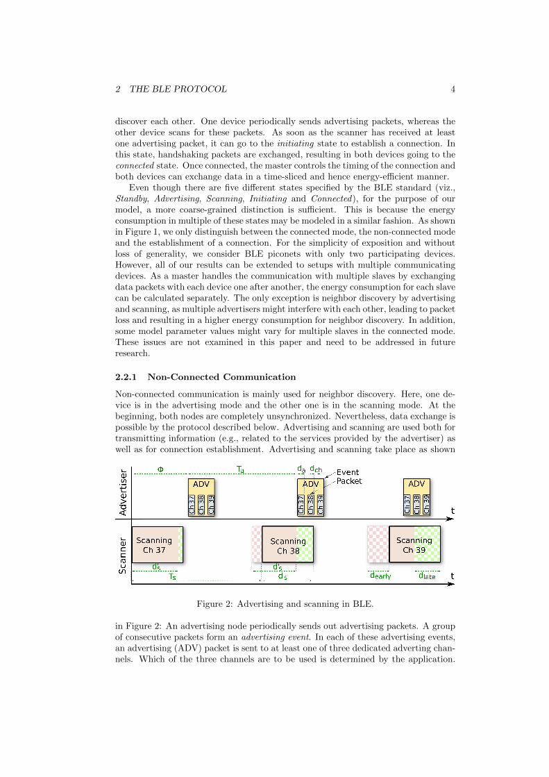
Figure 2: Advertising and scanning in BLE.
in Figure 2: An advertising node periodically sends out advertising packets. A groupof consecutive packets form an advertising event. In each of these advertising events,an advertising (ADV) packet is sent to at least one of three dedicated adverting chan-nels. Which of the three channels are to be used is determined by the application.

2 THE BLE PROTOCOL 5
Advertising events happen regularly with the advertising interval Ta. Independantfrom this, a scanner periodically switches on its receiver for a duration of ds timeunits called the scan window. This is repeated at every interval Ts, called the scaninterval. In the next period, the scanner hops to the next advertising channel andagain listens for advertising packets. The specification [13] requires the scanner to useall three advertising channels. If the scanner receives an advertising packet, it maysend a response packet to the advertiser within the same ADV-event. The advertiserexpects a response on the same advertising channel dIFS = 150µs after the end of theadvertising packet. dIFS is called the interframe-space. This enables the followingthree applications:
• Neighbor discovery: The scanner may respond to an advertising packet witha connection request packet. Both devices will then go into a connected mode,using the procedure described in Section 2.2.2.
• Broadcasting: The advertiser may send payload information within its ad-vertising packets. The scanner may receive them in a passive manner withoutresponding.
• Active scanning: If the scanner receives an advertising packet, it may send ascan-request-packet dIFS time units after the reception of an advertising packet,requesting more information to be sent by the advertiser another dIFS time unitslater.
The advertising interval is composed of a static interval Ta,0 and a random part ρ,i.e.,
Ta = Ta,0 + ρ,
where ρ is a random amount of time between 0ms and 10ms. The other timingparameters can be chosen by the host and are required to be within the followingtime intervals (some additional constraints depending on the mode of operation mightapply. We refer to the BLE specification [13] for details):
20ms < Ta,0 < 10.24s
0ms < Ts < 10.24s
0ms < ds ≤ Ts
The duration of an advertising event can be calculated in a manner similar to that ofcalculating the duration of a connection event in the connected mode. The modelingof these events is described in Section 4.2. The random offset ρ is added to Ta,0 toavoid the unfavorable case that Ts = Ta. In this case, if one advertising event missesa scan event, all subsequent advertising events would miss all future scan events tooand therefore the scanner would never discover the advertiser.
As the BLE protocol can be described as a temporal sequence of events, its result-ing energy consumption can be modeled by analyzing the energy consumption of itsevents and their frequency of occurrence. The energy model proposed in this paperfollows this reasoning.
2.2.2 Connection establishment
A connection can be established after a device has been detected by advertising/scanning.After having received at least one advertising packet, the scanner sends a connection-request packet dIFS time units later. This packet contains two parameters called
2 THE BLE PROTOCOL 6
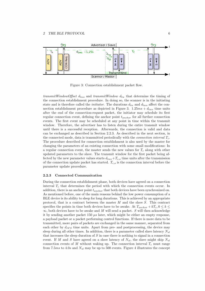
Figure 3: Connection establishment packet flow.
transmitWindowOffset dtwo and transmitWindow dtw that determine the timing ofthe connection establishment procedure. In doing so, the scanner is in the initiatingstate and is therefore called the initiator. The durations dtw and dtwo affect the con-nection establishment procedure as depicted in Figure 3. 1.25ms + dtwo time unitsafter the end of the connection-request packet, the initiator may schedule its firstregular connection event, defining the anchor point tanchor for all further connectionevents. The first event may be scheduled at any point in time within the transmitwindow. Therefore, the advertiser has to listen during the entire transmit windowuntil there is a successful reception. Afterwards, the connection is valid and datacan be exchanged as described in Section 2.2.3. As described in the next section, inthe connected mode, data is transmitted periodically with the connection interval Tc.The procedure described for connection establishment is also used by the master forchanging the parameters of an existing connection with some small modifications: Ina regular connection event, the master sends the new values for Tc along with otherupdated parameters to the slave. The transmit window for the first packet being af-fected by the new parameter values starts dtwo+Tc,o time units after the transmissionof the connection update packet has started. Tc,o is the connection interval before theparameter update procedure.
2.2.3 Connected Communication
During the connection establishment phase, both devices have agreed on a connectioninterval Tc that determines the period with which the connection events occur. Inaddition, there is an anchor point tanchor that both devices have been synchronized on.As mentioned before, one of the main reasons behind the low power consumption of aBLE device is its ability to sleep for long durations. This is achieved by an appropriateprotocol, that is a contract between the master M and the slave S . This contractspecifies the points in time both devices have to be awake. At Tanchor + kTc, 0 ≤ k ≤∞, both devices have to be awake and M will send a packet. S will then acknowledgeit by sending another packet 150 µs later, which might be either an empty response,a payload packet or a packet performing control functions. If there is more data to betransmitted, more pairs of packets are exchanged in the same manner, separated fromeach other by dIFS time units. Apart from pre- and postprocessing, the device maysleep during all other times. In addition, there is a parameter called slave latency Nslthat increases the sleep duration of S in case there is nothing to signal in a connectionevent. If M and S have agreed on a slave latency of Nsl, the slave might skip Nslconnection events of M without waking up. The connection interval Tc must rangefrom 7.5ms to 4.0s and Nsl may be up to 500 events. Figure 4 illustrates the concept
3 RELATED WORK 7
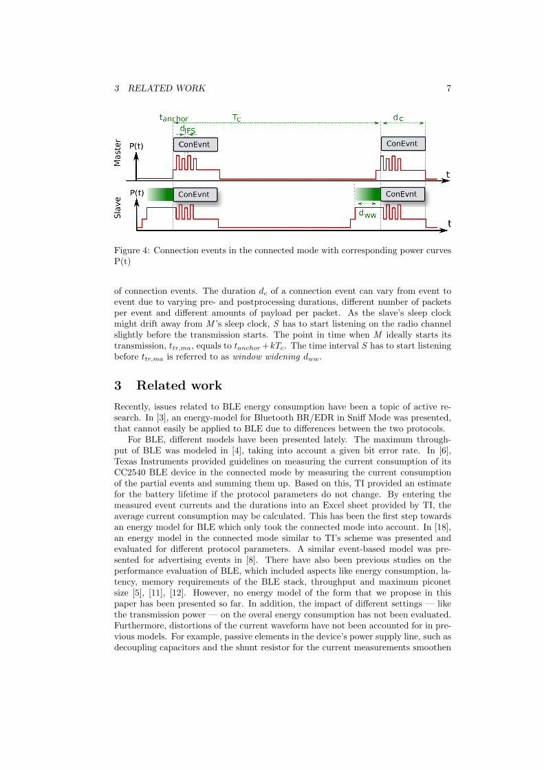
Figure 4: Connection events in the connected mode with corresponding power curvesP(t)
of connection events. The duration dc of a connection event can vary from event toevent due to varying pre- and postprocessing durations, different number of packetsper event and different amounts of payload per packet. As the slave’s sleep clockmight drift away from M ’s sleep clock, S has to start listening on the radio channelslightly before the transmission starts. The point in time when M ideally starts itstransmission, ttr,ma, equals to tanchor+kTc. The time interval S has to start listeningbefore ttr,ma is referred to as window widening dww.
3 Related work
Recently, issues related to BLE energy consumption have been a topic of active re-search. In [3], an energy-model for Bluetooth BR/EDR in Sniff Mode was presented,that cannot easily be applied to BLE due to differences between the two protocols.
For BLE, different models have been presented lately. The maximum through-put of BLE was modeled in [4], taking into account a given bit error rate. In [6],Texas Instruments provided guidelines on measuring the current consumption of itsCC2540 BLE device in the connected mode by measuring the current consumptionof the partial events and summing them up. Based on this, TI provided an estimatefor the battery lifetime if the protocol parameters do not change. By entering themeasured event currents and the durations into an Excel sheet provided by TI, theaverage current consumption may be calculated. This has been the first step towardsan energy model for BLE which only took the connected mode into account. In [18],an energy model in the connected mode similar to TI’s scheme was presented andevaluated for different protocol parameters. A similar event-based model was pre-sented for advertising events in [8]. There have also been previous studies on theperformance evaluation of BLE, which included aspects like energy consumption, la-tency, memory requirements of the BLE stack, throughput and maximum piconetsize [5], [11], [12]. However, no energy model of the form that we propose in thispaper has been presented so far. In addition, the impact of different settings — likethe transmission power — on the overal energy consumption has not been evaluated.Furthermore, distortions of the current waveform have not been accounted for in pre-vious models. For example, passive elements in the device’s power supply line, such asdecoupling capacitors and the shunt resistor for the current measurements smoothen
3 RELATED WORK 8
the waveform and modify the duration and amplitude of each part of the currentwaveform. As stated in [6], some parameters are subjected to random variations thatinfluence the power consumption. The impact of these variations on the total powerconsumption has not been evaluated yet. Instead, they have been assumed to beconstant. We have measured the variations of these parameters and incorporated themeasurements into our model. Finally, to the best of our knowledge, results fromany of the previously proposed models have not been compared to measured powercurves, bearing one exception for neighbor discovery presented in [8]. Consequently,the accuracy of these models was still not clear. Our measurements reveal that ourmodel is in close proximity with the measured current consumption. The highesterror for the average current consumption per connection interval we measured in ourexperiments was 6, 0%.
Besides from connected mode communication, neighbor discovery also contributesto the energy consumption. Energy models for this case are difficult to develop, asneighbor discovery is a stochastic process. Nevertheless, solutions to this problemhave been presented: In the protocol STEM-B, neighbor discovery is done in a sim-ilar way as in BLE. A model for this was presented in [17] and applied to BLE in[8], [10] and [9], predicting the energy-consumption of the advertiser in a neighbordiscovery process. However, it has been stated in [9] that this model is only valid fora certain range of possible parameter values (Ta < ds or Ts = ds as defined in Section2). In [8], measurements comparing modeled and measurement energy consumptionhave been performed for the neighbor discovery model proposed in that paper. Formodeling the energy consumed during neighbor discovery, an energy model consistingof partial events for advertising, similar to the one in [6] has been used.
Our contributions: In this paper, we propose a comprehensive energy model ofthe BLE protocol, modeling the energy consumption for all operation modes and forall possible parameter valuations. Towards this, we integrate a number of previouslyknown models and at the same time refine and extend them in order to obtain a com-plete model that accounts for all possible modes of communication with all possibleparameters. In particular, our contributions are as follows.
1. To the best of our knowledge, we present the first model that includes i) allpossible modes of operation, ii) all relevant parameters, and iii) all possibleparameter valuations of the BLE protocol. For example, in the connected mode,our model takes into account the distortion of the current curve caused byresistive and capacitive elements present in the power supply line. Instead ofrelying on theoretical data from the BLE specification [13] and values fromdevice data sheets only, our model includes measured durations and currentmagnitudes, leading to more accurate predictions on state durations comparedto previous models. For example, in our model the duration of the transmissionstate is modeled as a constant part and a part depending on the number of bytessent rather than a byte-dependent duration only. In addition, we present thefirst model for scan events, for connection setup and for updating the connectionparameters. We are also the first to present an algorithm that estimates thediscovery latency and energy consumption for neighbor discovery for all possibleparameter values, including Ta > ds. Analytical solutions exist only for Ta < ds[8]. Based on the proposed model, we present guidelines to system designers fordetermining protocol parameter values that optimize the power consumptionfor different application scenarios.
4 BLE POWER MODEL 9
2. Using multiple measurements, we identified the degree of variation in the val-uation of the different parameters and the sensitivity of these parameters onthe total energy consumption. In many cases, it is reasonable to use meanvalues of varying parameters, but sometimes this is insufficient. For example,when estimates on maximum current consumptions over small time intervalsare necessary, identifying a range over which the parameter varies is required.In a sensitivity analysis, we investigated the impact of these variations on theoverall power consumption. In addition, we analyzed the impact of differenttransmission-power-settings on the energy consumption.
3. To the best of our knowledge, none of the known energy models for BLE havebeen compared to measured data yet, bearing one exception presented in [8],where the energy consumption of an advertiser for neighbor discovery was mod-eled and compared to measured data. We have validated the results from ourproposed model with real experimental results. Therefore, we performed com-parative measurements for the modeled neighbor discovery latency to prove thatour results are in very close proximity to the measured data. In measurementswe performed for the connected mode, the modeled mean current consump-tion within a connection interval differed from the measured results by between1.17% and 6.0%.
4 BLE Power Model
In this section, we present a precise energy model for BLE that is capable of predictingthe energy-consumption of the protocol in all modes of operation.
4.1 Overview
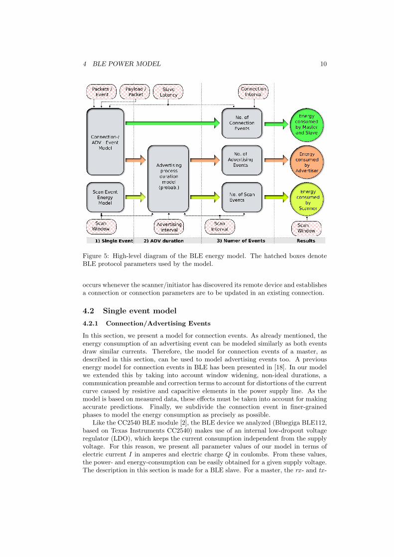
Figure 5 gives an overview on our approach. The BLE protocol can be modeled as atemporal sequence of single events that happen periodically. Energy models of theseevents depend on their type (connection- , advertising- or scan-event), as can be seenon the left in Figure 5. The hatched boxes in the figure depict protocol parametersthat are fed into the model.
In Stage 1) of Figure 5, the energy of all single events that occur is modeled. InStage 2), the average duration of an advertising/scanning-process dadv is modeled forthe advertising/scanning mode. This duration is of stochastic nature. It determineshow often an advertising event or scan event has to be repeated before the data(either payload or handshaking for the initialization of a connection establishmentprocess) has successfully been received at the receiving node. In the connected mode,this time is deterministic and is defined by the connection interval Tc and the slavelatency parameter Nsl. In the third stage, the number of identical events that occurwithin a certain amount of time is calculated. Next, the energy consumed per eventis multiplied by the number of times it occurs and the results for different events arethen summed up. In addition, the time the device sleeps between these events and itscorresponding sleep energy consumption is calculated. By combining the energy ofall events with the energy spent during sleeping, the expected energy for transmittinga given payload for a given set of parameters can be calculated. In this section, wedescribe every block in Figure 5. In addition, we describe an energy model for theconnection establishment procedure, which is not shown in the figure. This procedure
4 BLE POWER MODEL 10
Figure 5: High-level diagram of the BLE energy model. The hatched boxes denoteBLE protocol parameters used by the model.
occurs whenever the scanner/initiator has discovered its remote device and establishesa connection or connection parameters are to be updated in an existing connection.
4.2 Single event model
4.2.1 Connection/Advertising Events
In this section, we present a model for connection events. As already mentioned, theenergy consumption of an advertising event can be modeled similarly as both eventsdraw similar currents. Therefore, the model for connection events of a master, asdescribed in this section, can be used to model advertising events too. A previousenergy model for connection events in BLE has been presented in [18]. In our modelwe extended this by taking into account window widening, non-ideal durations, acommunication preamble and correction terms to account for distortions of the currentcurve caused by resistive and capacitive elements in the power supply line. As themodel is based on measured data, these effects must be taken into account for makingaccurate predictions. Finally, we subdivide the connection event in finer-grainedphases to model the energy consumption as precisely as possible.
Like the CC2540 BLE module [2], the BLE device we analyzed (Bluegiga BLE112,based on Texas Instruments CC2540) makes use of an internal low-dropout voltageregulator (LDO), which keeps the current consumption independent from the supplyvoltage. For this reason, we present all parameter values of our model in terms ofelectric current I in amperes and electric charge Q in coulombs. From these values,the power- and energy-consumption can be easily obtained for a given supply voltage.The description in this section is made for a BLE slave. For a master, the rx - and tx -

4 BLE POWER MODEL 11
Figure 6: Model for a BLE connection event of a slave device.
phases described below are interchanged and no window-widening occurs. Therefore,the model described can be used for a BLE master too.
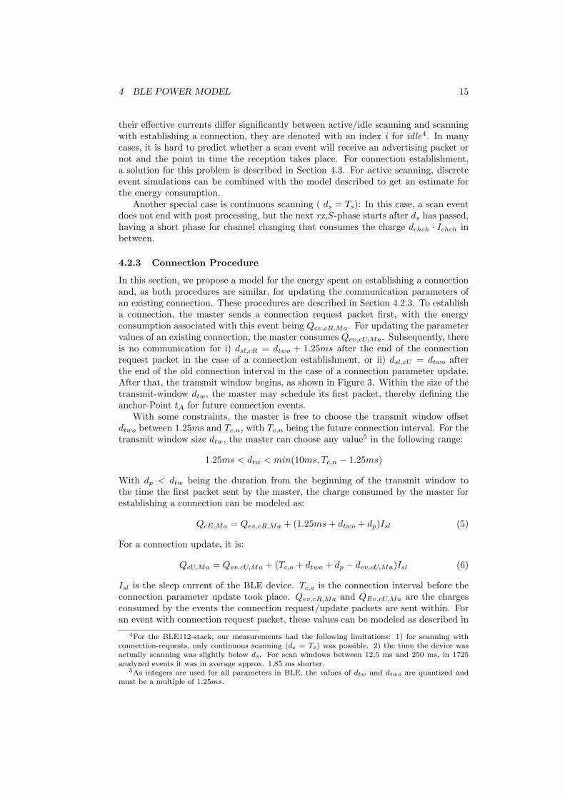
Within a connection event, ten distinguishable phases with nearly constant currentconsumptions can be identified. As shown in Figure 6, these phases are as describedbelow.
1. Header (head): At the beginning of a connection event, the device wakes up.Thereby, a current Ihead is consumed for the duration of dhead.
2. Preprocessing (pre): Prior to the actual communication, the device wakes upand prepares the functions related to the BLE standard, which are used duringthe communication, such as the logical link control and adaptation protocol(L2CAP), generic access profiles (GAP), generic attribute profile (GATT), se-curity manager (SM), etc. While the average current is nearly constant overtime during this phase, its duration might vary depending on the BLE device,the BLE stack and the BLE functionality that is used (.e.g., sending attributeswith or without confirmation). In addition, random variations occur, as can beseen in the tables of Appendix A.
3. Communication preamble (cpre): The wireless communication is initiatedin this phase. It is inherent to the hardware and its current and duration maychange with different BLE device models.
4. Window widening (ww): As already mentioned, the slave has to start listen-ing for a certain amount of time before the master starts sending its first packetto compensate for the time drift that might be generated due to clock skews.This additional time is called window widening dww. It depends on the nominalsleep clock accuracy (SCA) of each transceiver, the connection interval Tc andthe average slave latency Nsl as shown in Equation 4. The sleep clock is theclock that determines the points in time for waking up a sleeping device. Thecurrent magnitude of this phase is the same as the magnitude of the rx -phase.The duration dww can be calculated according to Equation 4 [13], assuming thatthe average clock skew is equal to zero (positive and negative skew compensatefor each other).
dww =(SCAMa + SCASl) · Tc ·Nsl
106, Iww = Irx (1)

4 BLE POWER MODEL 12
5. Reception (rx): The over-the-air-bitrate of BLE is specified to be 1 MBits/s,therefore one bit is transmitted within 1µs. Consequently, the rx -phase shouldideally take Nrx · 8µs, with Nrx being the number of bytes received. Becausethe RF circuitry needs some time to initialize, the duration of the rx -phase isslightly longer than its ideal value. To account for this, a correction-offset dprerxis added to drx as in the equation below.
drx = Nrx · 8µs+ dprerx.
The current Irx is nearly constant; some devices such as the CC2540 [16] havemultiple reception-gain settings that cause different current draws.
6. Interframe-Space (rxtx, txrx): After the rx -phase and before the slave startssending a packet to the master, there is a phase for switching from reception totransmission and vice-versa. Its duration is slightly shorter than the over-the-airgap between two packets dIFS .
7. Transmission(tx): In this phase, the slave transmits data to the master. Itsduration can be modeled in a manner similar to the rx -phase using Equation 7.
dtx = dpretx +Ntx · 8µs (2)
Ntx is the number of bytes transmitted. The current consumption Itx dependson the tx -power that is used. For a BLE112-device, there are 15 different tx -power-settings. In addition, Itx slightly varies with the channel a packet is senton. As the channel is determined by a pseudo-random hopping sequence, thesevariations can be assumed to occur randomly with a given standard deviation.The BLE protocol allows the transmission of multiple pairs of packets in a singleconnection event. After another txrx -phase, the rx, rxtx and tx -phases mightbe repeated to account for multiple pairs of packets.
8. Tx transient (tra): After the data transmission has ended, the current de-creases from Itx to the postprocessing-current Ipost. Whereas the current con-sumption drops with a RC curve, an effective constant current Itra and aneffective duration dtra can be chosen appropriately to take the charge consumedby this into account.
9. Postprocessing (post): After the communication has ended, the device mayexecute additional tasks such as wired communication to a host processor ordata buffering for the next transmission. Therefore, the duration of this phaseis strongly dependent on the BLE device and its software. In our experi-ments, we measured the post-processing duration caused by a firmware createdwith Bluegiga’s BGScript [1] without accounting for additional tasks. Both onBLE112- and CC2540-devices, dpost is subjected to strong random variations[6]. When executing one BLE functionality (e.g., sending a packet), we mea-sured varying postprocessing times as presented in the tables in Appendix A.Correlations between dpre and dpost might exist. In [6] it is stated that for aCC2540-device, the sum of dpre and dpost is always the same. In our measure-ments for a BLE112-device, we could not reproduce this behavior2. For ourmodel, we assume that there is no correlation between dpre and dpost. If pre-cise predictions on short-time currents need to be done, one should analyze thecorrelations of these durations for the device used.
2For example, the sum of dpre and dpost varied for different numbers of packets per event.

4 BLE POWER MODEL 13
10. Tail (tail): After the BLE device has completed the tasks related to the post-processing, it goes to a sleep mode to reduce the energy consumption. Thisphase in the model accounts for the current consumed for initiating the lowpower mode.
The timing for these phases differ for the over-the-air traffic and the current-curvemeasured. The values needed for an energy-model consider the timing of the currentdraw.
For each phase ph, the charge consumed can be calculated by Qph = dphIph.With the phases described, the charge consumed for a connection event, QcE , can becomputed as in Equation 4.2.1.
QcE = Qhead +Qpre +Qcpre +Qww +Qt +Qtra +Qpost +Qtail (3)
Qt accounts for the actual communication taking place. For a communication withNseq pairs of packets, it is
Qt =
Nseq∑i=1
(Qrx(i) +Qtx(i) +Qrxtx +Qtxrx +Qto)−Qtxrx
Qto is an offset to account for distortions in the current curve. Due to the distortion ofthe current curve caused by resistive and capacitive elements in the power supply line,the shape of the phases of the current curve are not perfectly rectangular. This can becompensated with effective parameter values for event-phases with constant length.In contrast, for the communication sequence, an offset term needs to be added asthe varying durations make it impossible to find effective values accounting for offsetsthat occur.
The duration of a connection event can be calculated similar to Equation 4.2.1 byadding the partial durations of all phases.
4.2.2 Scan Event
The current waveform of a scan event depends on the mode the device is in. Possiblemodes are described in Section 2.2.1. We describe the energy consumption for an eventwith active scanning, which is the most complex waveform, and simplify it for eventswith no reception of data and for events which receive connection-request packets. In
Figure 7: Current waveform of a scan event when receiving and serving a scan requestpacket (active scanning)
.
the equations in this section, paramters denoted with an s indicate scanning, as the

4 BLE POWER MODEL 14
parameter values differ from the values in the connected mode. Figure 7 shows thecurrent-waveform for active scanning, assuming that exactly one advertising event isreceived during one scan event. As for the connection event, the device wakes up,drawing a current for the duration of dpre,s
3. Afterwards, it scans for the scanningtime dS,1 until an incoming advertising packet is received, consuming a high currentIscan = Irx,s due to the permanent usage of the receiver circuit. During the receptionof the packet, the current consumption remains the same. The device then switchesfrom receiving to transmission, which takes drxtx,s amounts of time. Next, it sendsa scan request packet lasting for dtx,s = Ntx · 8µs + dpretx,s time units. Here, Ntxis the number of bytes sent and dpretx,s is a correction offset accounting for chargingand discharging capacitances. Afterwards, the devices switches from tx to rx, takingthe time dtxrx,s and subsequently, a scan response packet from the remote device isreceived. This takes drxsr = Nrx ·1µs+dprerx,s time units. Before the device continuesscanning, there is a phase with constant current for drxrx,s units of time. When thetime dS,2 has expired, the device stops scanning and goes to sleep, consuming asmaller current for the time dpost,s before the sleep phase begins. The scan durationsdS,1 and dS,2 depend on the time an advertising packet is received and hence arerandom. Fortunately, for calculating the energy consumption, only the sum of dS,1and dS,2 is of interest, which is given by the scan window ds. It is approximatelydscan = ds−drxtx,s−dtx,s−dtxrx,s−drxsr−drxrx,s. Therefore, the charge consumedby a scan event with active scanning is:
QsEv =dpre,s + dscanIrx,s + drxtx,sIrxtx,s + dtx,sItx,s + dtxrx,sItxrx,s + drxsrIrx,s
+drxrxIrxrx + dpost,sIpost,s +Qcrx,s +Qctx,s (4)
Qcrx,s and Qctx,s are correction offsets to compensate for non-rectangular shapesin the reception and transmission phases. Parameter values for Equation 4.2.2 forBLE112-devices are presented in Appendix A. In many cases, this equation can besimplified. For sending a connection request packet, the waveform begins similarto what is shown in Figure 7 but instead of a scan-response packet, a connectionrequest packet is sent. In this case, the tx -phase is followed by the postprocessingphase without further sections in between. Our experiments showed that the pre-and post-processing phases for scanning with a connection request last longer thanfor active scanning on a BLE112-module. This behavior depends on the device andits BLE stack. For the sake of simplicity of explanation, we nevertheless assume thesedurations to be constant in the values presented in this paper, as this could easilybe accounted for by adjusting the values to the given case. Because of the reducednumber of phases in the case a connection is initiated, drxtx,s, drx,s, Qcrx,s and drxrx,scan be set to zero and dscan is shortened to the time between the beginning of theidle scanning and the time the advertising packet has been received completely. Ifno advertising packet is received or only passive scanning is used, there is only idle-scanning (or the reception of advertising-packets that consumes the same energy asscanning) and the charge consumed can be computed in a simplified way:
QsEv,Idle = dpre,s,iIpre,s,i + dpost,s,iIpost,s,i + dsIrx
If ds is long compared to dpre+dpost, pre- and postprocessing can be neglected and theformula above can be simplified further. As pre- and postprocessing-durations and
3We denote the phase at the beginning of a scan event as the preprocessing phase and the phase atthe end of a scan event as the postprocessing phase. This does not mean that the device necessarilydoes data processing in these phases.
4 BLE POWER MODEL 15
their effective currents differ significantly between active/idle scanning and scanningwith establishing a connection, they are denoted with an index i for idle4. In manycases, it is hard to predict whether a scan event will receive an advertising packet ornot and the point in time the reception takes place. For connection establishment,a solution for this problem is described in Section 4.3. For active scanning, discreteevent simulations can be combined with the model described to get an estimate forthe energy consumption.
Another special case is continuous scanning ( ds = Ts): In this case, a scan eventdoes not end with post processing, but the next rx,S -phase starts after ds has passed,having a short phase for channel changing that consumes the charge dchch · Ichch inbetween.
4.2.3 Connection Procedure
In this section, we propose a model for the energy spent on establishing a connectionand, as both procedures are similar, for updating the communication parameters ofan existing connection. These procedures are described in Section 4.2.3. To establisha connection, the master sends a connection request packet first, with the energyconsumption associated with this event being Qev,cR,Ma. For updating the parametervalues of an existing connection, the master consumes Qev,cU,Ma. Subsequently, thereis no communication for i) dsl,cR = dtwo + 1.25ms after the end of the connectionrequest packet in the case of a connection establishment, or ii) dsl,cU = dtwo afterthe end of the old connection interval in the case of a connection parameter update.After that, the transmit window begins, as shown in Figure 3. Within the size of thetransmit-window dtw, the master may schedule its first packet, thereby defining theanchor-Point tA for future connection events.
With some constraints, the master is free to choose the transmit window offsetdtwo between 1.25ms and Tc,n, with Tc,n being the future connection interval. For thetransmit window size dtw, the master can choose any value5 in the following range:
1.25ms < dtw < min(10ms, Tc,n − 1.25ms)
With dp < dtw being the duration from the beginning of the transmit window tothe time the first packet sent by the master, the charge consumed by the master forestablishing a connection can be modeled as:
QcE,Ma = Qev,cR,Ma + (1.25ms+ dtwo + dp)Isl (5)
For a connection update, it is:
QcU,Ma = Qev,cU,Ma + (Tc,o + dtwo + dp − dev,cU,Ma)Isl (6)
Isl is the sleep current of the BLE device. Tc,o is the connection interval before theconnection parameter update took place. Qev,cR,Ma and QEv,cU,Ma are the chargesconsumed by the events the connection request/update packets are sent within. Foran event with connection request packet, these values can be modeled as described in
4For the BLE112-stack, our measurements had the following limitations: 1) for scanning withconnection-requests, only continuous scanning (ds = Ts) was possible. 2) the time the device wasactually scanning was slightly below ds. For scan windows between 12,5 ms and 250 ms, in 1725analyzed events it was in average approx. 1,85 ms shorter.
5As integers are used for all parameters in BLE, the values of dtw and dtwo are quantized andmust be a multiple of 1.25ms.

4 BLE POWER MODEL 16
Section 4.2.1 as an advertising event with 37 bytes sent by the advertiser and witha response of 44 bytes length sent by the scanner(i.e., connection-request packet).Connection update requests can be modeled as a connection event with a 22-bytepacket sent by the master and packets received from the slave depending on thepayload the slave has to send.
The master’s energy-consumption mainly stems from sending the connection re-quest/update packet to the slave. Opposed to that, the energy consumption of theslave is dominated by the current of its receiver during idle-listening in the transmitwindow and during the reception of the packet. It can be modeled by the followingequations:
QcE,S = Qev,cR,Sl + (dtwo + 1.25ms− dww,cE)Isl + (dp + dww,cE)Irx
and
QcU,S = Qev,cU,Sl + (Tc,o + dtwo − dww,Cu − dev,cU,Sl)Isl + (dp + dww,cU )Irx
Qev,cR,Sl/dev,cR,Sl and Qev,cU,Sl/dev,cU,Sl are the charges/durations consumed by theevents where the connection request is sent/connection update-packet is receivedwithin. As Qev,cR,Sl is a scan event, it can be modeled according to Section 4.2.2,whereas Qev,cU,Sl is a connection event and therefore can be modeled according toSection 4.2.1. Irx is the current consumption when the receiver listens to the radiochannel. The first connection event after this procedure has to be modeled withoutwindow widening as the equations above already account for it. Due to possible clockskew on both devices, window widening occurs that broadens the transmit windowand therefore the duration the current Irx is drawn. dww,cE and dww,cU contain thetimes the transmit window is broadened by. With SCAMa and SCASl being theclock accuracies of master and slave in parts per million, the window-widenings forconnection establishment dww,cE and for connection parameter updates dww,cU are:
dww,cE =SCAMa + SCASl
1000000(1.25ms+ dtwo)
dww,cU =SCAMa + SCASl
1000000(Tc,o + dtwo)
In Equations 4.2.3 and 4.2.3, we neglected the fact that the sleep duration is slightlyshorter than what has been modeled, as the first event after the connection estab-lishment or update sequence overlaps with the sleep duration (e.g. header, prepro-cessing, communication preamble). However, due to the small sleep current of BLEdevices, the impact of this is low. The values of dtw, dp, dtwo are chosen freely by theBLE stack and are therefore unknown, making the equations above hard to evaluate.However, a worst case-model can be defined. Both for the master and the slave, themaximum energy is consumed if both parameters have their maximum values, viz.dp = min(10ms, Tc,n − 1.25ms) and dtwo = Tc,n. Moreover, even if not explicitly de-fined by the BLE specification, some assumptions on the values of these parameterscan be made for real-world devices, that lead to an estimation of the average energyconsumed for establishing a connection or updating the connection parameters. Bothparameters are used to allow the master to schedule a new anchor point ta. At thispoint in time, the first connection event of the new/updated connection starts. Usingdtwo, the first connection event can be scheduled if it is already known at the timethe master sends the connection request/update packet to the slave. In addition,

4 BLE POWER MODEL 17
dtw leaves open a time interval for the master to schedule the anchor point withoutdetermining it when sending the connection request or update packet. As there is noreason for the master for not being able to schedule tAnchor already when sending theconnection parameters to the master, we assume that it will choose a small values ofdtw. We further assume that every point in time within the transmit window is takenwith the same likelihood. Hence, on an average the master will schedule tA at themiddle of this interval, i.e. dp = dtw
2 . If the master choses small transmit windowsttw, there is a clear benefit for its energy consumption and as a consequence, a goodBLE stack is likely to do so. However, making reasonable assumptions for the valueof dtwo is more difficult. dtwo only influences the charge spent by sleeping and bywindow widening. The energy consumption related to this is expected to be smallagainst the energy consumed for idle-listening within dtw and for receiving a packet.From an energy-perspective, the BLE stack can chose an arbitrary value. For energymodeling, dtwo can be assumed to have its maximum value Tc,n if the actual value ofthe device is unknown.
Whereas a coarse estimation of the energy consumed by the procedure describedcan be made using these assumptions, for more precise energy estimations, the param-eters actually chosen by the BLE stack considered need to be analyzed. We observedthe values used by the stack of a CC2540-based BLE112-device manufactured byBluegiga, by using a Texas Instrument’s packet sniffer software [15]. A passive BLEdevice was used to wiretap the BLE traffic between two different communicating de-vices. We developed a parser for the logs generated by the SmartRF Packet Sniffersoftware [15], allowing for the import of the sniffed data into MATLAB.
By manually experimenting different parameter values, we found that dtw = 3ms isconstant for all parameter values in all situations. We further analyzed 26 connectionprocedures, where dp had an average value of 1.43ms which is close to dtw
2 , as weassumed. dtwo may vary for different values of TC when establishing a new connection,while being constantly equal to zero for connection updates. We developed a softwarethat repeatedly connects and disconnects two BLE nodes. The packet-sniffer-logswere analyzed to obtain dtwo for different values of Tc. An analysis of about 12,000connection procedures revealed the following result for a BLE112-device: dtwo growswith increasing values of Tc, but there are some random variations for the same valueof Tc. For Tc > 12.5ms, an estimation for dtwo is:
dtwo = Tc − 6.454ms (7)
The maximum deviation that occurred in all the measurements was 6.046ms (0.87%of the corresponding measured value), the mean square error was 8.756µs and thestandard deviation σ was 2.959ms. These results show that Equation 4.2.3 is a goodestimation of dtwo. For 7.25ms < Tc < 12.5ms, a good estimation for dtwo is:
dtwo = 0.389Tc + 0.484ms (8)
The mean square error in our measurements for Equation 4.2.3 is 6.322µs, the stan-dard deviation σ is 2.527ms, the maximum deviation that occurred is 5.140ms (51.4%of the corresponding measured value). These values are valid for BLE112-devices inpiconets with one slave. For other situations or different hardware, this measurementhas to be performed again using the procedure we described. It would be desirable ifthe manufacturers of BLE stacks would publish data concerning the values of dtwo anddtw in future, as this information might be important for online power managementalgorithms on BLE devices.
4 BLE POWER MODEL 18
The connection establishment procedure is always associated with advertising andscanning. Therefore, the charges Qev,cR,Sl and Qev,cR,Ma need to be assigned eitherto the connection establishment model or to the neighbor discovery model. By defi-nition, we assign it to the neighbor discovery model, accounting for them as the lastadvertising or scan-event event happening and therefore, set it to zero in the equationsdescribed in this section to avoid counting these charges twice.
4.3 ADV process duration
Advertising and scanning in Bluetooth Low Energy were described in Section 2.2.During these phases, the advertiser (A) is not synchronized with the scanner (S) andthe reception of a packet sent to the scanner by A is not guaranteed. Instead, thetime when a scanner receives an advertising packet can be described as a stochasticprocess, and it is likely that the advertiser will have to send a packet more than oncebefore it is received by the scanner. This stochastic nature has a strong impact onthe energy consumption of the BLE device in this mode, as a packet has to be sentmultiple times and the scanner has to scan until a successful reception is achieved.
In many cases, the energy-consumption for device discovery is dominated by theenergy spent in advertising or scanning mode without a successful reception. There-fore, the number of advertising events Na and scan events Ns that take place inaverage before a successful reception occurs have to be calculated. To do this, wederive the average duration of this process dadv. It is defined as the time from thefirst advertising packet being sent until there is a successful reception at the scannerand is closely related to the number of events6.
In this section, we first present a probabilistic model for estimating dadv. Itdepends on the protocol parameters Ta, Ts, ds and the duration of one advertisingpacket dadvPkg, which is calculated in Section 4.2. Recall from Section 2 that thescanner hops between all the three advertising channels and stays on one channel foreach scan window ds, whereas the advertiser may freely choose a set of advertisingchannels to send its packets on. In this section, we assume that the advertiser sendspackets on all three advertising channels. Results for cases when only a subset ofchannels are used can be calculated in a similar manner.
4.3.1 Problem description
Figure 2 shows a typical advertising/scanning situation. A scanner S starts listeningat its first scan event at time t = 0. An advertiser A begins advertising after a randomdelay φ relative to the beginning of the first scan event. It periodically repeats itsadvertising event with period Ta = Ta,0 + ρ, whereby ρ is a random offset between0ms and 10ms. The relevant question that needs to be answered is the following.How much time will pass, until an advertising event “meets” a scan event for the firsttime, or in other words, what is the earliest time when the two events coincide?
A condition for successful reception needs to be identified. An advertising eventis received by the scanner, if its starting time ta is contained within a set of suitabletimes ti,suc. On first glance, ti,suc appears to contain all points in time where theadvertising time begins while the node is scanning. Indeed, an advertising eventmight start even earlier than the subsequent scan event, to be received successfully.In addition, some points in time within a scan event lead to a lost advertising packet.The hatched areas in Figure 2 on the left side of the scan events show the possible
6We assume that the scanner has already been scanning when the advertiser starts advertising.
4 BLE POWER MODEL 19
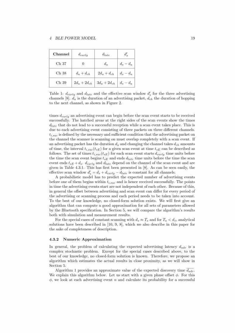
Channel dearly dlate d′s
Ch 37 0 da ds − da
Ch 38 da + dch 2da + dch ds − da
Ch 39 2da + 2dch 3da + 2dch ds − da
Table 1: dearly and dlate and the effective scan window d′s for the three advertisingchannels [8]. da is the duration of an advertising packet, dch the duration of hoppingto the next channel, as shown in Figure 2.
times dearly an advertising event can begin before the scan event starts to be receivedsuccessfully. The hatched areas at the right sides of the scan events show the timesdlate that do not lead to a successful reception while a scan event takes place. This isdue to each advertising event consisting of three packets on three different channels.ti,suc is defined by the necessary and sufficient condition that the advertising packet onthe channel the scanner is scanning on must overlap completely with a scan event. Ifan advertising packet has the duration da and changing the channel takes dch amountsof time, the interval ti,suc(tsE) for a given scan event at time tsE can be described asfollows. The set of times ti,suc(tsE) for each scan event starts dearly time units beforethe time the scan event begins tsE and ends dlate time units before the time the scanevent ends tsE + ds. dearly and dlate depend on the channel of the scan event and aregiven in Table 4.3.1. This has first been presented in [8]. As can be seen easily, theeffective scan window d′s = ds + dearly − dlate is constant for all channels.
A probabilistic model has to predict the expected number of advertising eventsbefore one of them begins within ti,suc and is hence received successfully. The pointsin time the advertising events start are not independent of each other. Because of this,in general the offset between advertising and scan event can differ for every period ofthe advertising or scanning process and each period needs to be taken into account.To the best of our knowledge, no closed-form solution exists. We will first give analgorithm that can compute a good approximation for all sets of parameters allowedby the Bluetooth specification. In Section 5, we will compare the algorithm’s resultsboth with simulation and measurement results.
For the special cases of constant scanning with ds ≈ Ts and for Ta < ds, analyticalsolutions have been described in [10, 9, 8], which we also describe in this paper forthe sake of completeness of description.
4.3.2 Numeric Approximation
In general, the problem of calculating the expected advertising latency dadv is acomplex stochastic problem. Except for the special cases described above, to thebest of our knowledge, no closed-form solution is known. Therefore, we propose analgorithm which estimates the actual results in close proximity, as we will show inSection 5.
Algorithm 1 provides an approximate value of the expected discovery time dadv.We explain this algorithm below. Let us start with a given phase offset φ. For thisφ, we look at each advertising event n and calculate its probability for a successful

4 BLE POWER MODEL 20
reception phit(n), given that all previous events have not been received at the scanner.Without the random advertising delay ρ, the probability would be estimated to either0 or 1 - if the advertising begins within ti,suc, it is 1, for all other cases, it is 0. Witha random offset ρ, the time an advertisement event begins, tadvEvt, can lie withina broad time interval which widens for increasing event numbers n. Therefore, phitdepends on n. ρ is modeled as a random variable ρ, having the distribution
f(ρ) =
1
10ms if 0 ≤ ρ ≤ 10ms
0 , else(9)
As the Bluetooth specification [13] only specifies the possible range of values for ρbut not its distribution, this is a further assumption. As ρ is generated by a digitalrandom number generator (RNG) and digital RNGs commonly produce uniformlydistributed values, this assumption should hold true for most devices. The time anadvertising event begins tadvEvt can be modeled as in Equation 4.3.2:
tadvEvt(n, φ) = φ+ nTa︸ ︷︷ ︸A
+
n∑1︸︷︷︸B
ρ (10)
For calculating the probability phit of weather an advertising event is successfullyreceived, the probability density function (PDF) of the start of an advertising eventover time tadvEvt(n, φ) is required. In Term B in Equation 4.3.2, the shape of thedistribution depends on n. For n = 1, the distribution is uniform as assumed. Asn random offsets ρ occur, the resulting distribution can be described as the sum ofn independent and identical random variables ρ. In general, the PDF of a sum ofn random variables is the convolution product of their PDFs [19]. According to thecentral limit theorem for large n, the convolution product passes into a Gaussiandistribution having the effective mean µ′ = nµ and the effective standard deviationσ′ = nσ [19]. Accordingly, for the distribution f(B) of B, we assume a Gaussiandistribution with the mean µρ = n · 5ms and standard deviation σρ =
√n12 · 10ms for
an arbitrary n > 2. For n = 1, the uniform distribution from Equation 4.3.2 is used.For n = 2, we assume the distribution to be a symmetric triangular distribution withf(B) = f(ρ) ∗ f(ρ) (the exact solution of the convolution product). For the ease ofexposition, in this section, a Gaussian distribution is assumed for n = 1 and n = 2,too. However, the values we present in this paper have been calculated withoutusing this simplification. To further increase the accuracy of the results, one maypre-calculate the convolution functions for the first n advertising events and use theGaussian distribution only for large values of n7.
The Term A in Equation 4.3.2 causes a shift in the mean of f(phit). The approx-imate distribution for the time tadvEvt(n, φ) is:
f(tadvEvt(n, φ)) = Φ(φ− nTa − n · 5ms√
n12 · 10ms
)
Φ(t) is the cumulative distribution function of the standard normal distribution.Therefore, phit can be calculated as in Line 10 in Algorithm 1 by evaluating f(tadvEvt(n, φ))for all scan intervals k the beginning of the advertising event tadvEvt(n) might liewithin. The first scan event that might receive the advertising event n is given by
7Our experiments have shown that using Gaussian PDFs for n > 2 provides sufficient accuracy.
4 BLE POWER MODEL 21
kmin and the last possible one is scan event number kmax. The indices kmin and kmaxcan be calculated with the formulas in Line 5 of the algorithm. With tai being theideal point in time an advertising-event starts (i.e. without the random advertisingdelay ρ), pk in Line 10 can be calculated. pk(k, n, tai, dearly, dlate, Ts) is the probabil-ity for the advertising event n being received successfully by the scanner. It can becalculated as follows.
pk = Φ(kTs + ds − dlate − tai − n · 5ms√
n12 · 5ms
)− Φ(kTs + dearly − tai − n · 5ms√
n12 · 5ms
)
Thus, the expected advertising duration for a given offset φ can be calculated asin Line 11 of the algorithm. pcM (n) is the probability that n advertising events do notlead to a successful reception (cumulative miss probability). In Line 13 of Algorithm1, the probability for n cumulative misses is calculated for the current advertisingevent. dexp in Line 11 is a good approximation of the exact8 expected advertisingduration, which would be:
dexp =
kTs+ds−dlate∫kTs−dearly
Φ(t, tai + n10ms
2,
√n
1210ms)
since this equation is computationally complex and the benefit in terms of accuracyis small, the expected value of ρ (i.e., 5ms) is used in the algorithm and the error canbe neglected.
With increasing values of n, the probability that one of the advertising eventsconsidered until so far is received successfully grows. Consequently, pcM shrinks withgrowing n. The algorithm finishes, if (1− pcM ) is smaller than a lower bound ε. Thehigher ε is, the better the accuracy of the algorithm becomes, but the correspondingcomputational complexity increases.
Following the steps described above, the resulting values of dexp must be integratedover all possible values of φ. We perform a simple numerical integration by evaluatingthe integral for φ ∈ [0, 3 · Ts] in steps of ∆, multiplying the results with ∆ andcomputing the sum of these values. The variable ch contains the value of the currentchannel the scanner receives on and is calculated in Line 8 of the algorithm. Thefunction getInterval(ch) used in the algorithm looks up dearly and dlate from Table4.3.1. The function dadvEvnt(ch) calculates the duration of an advertising event whichis received successfully by the scanner on the current channel as described in Section4.2.1. For channel 37 this is da, for channel 38 it is 2da + dch and for channel 39 it is3da + 2dch.
In order to bound the computation time, the inner while-loop of Algorithm 1should be aborted if dexp exceeds an upper bound dexp,max. In practice, this is not areal limitation because parameterizations leading to advertising durations larger than,for example, dexp,max = 1000s are no reasonable choices for real world applications.The long latencies resulting from such parametrizations cannot be accepted and arenot pareto-optimal. The algorithm has two parameters ε and ∆ that influence thequality of the result. The smaller ∆ is and the closer ε gets to 1, the more accuratethe result becomes. Compared to discrete event simulations, this algorithm has areduced complexity when choosing these values appropriately, as not all scan events
8Exact means the value under all assumptions made so far.
4 BLE POWER MODEL 22
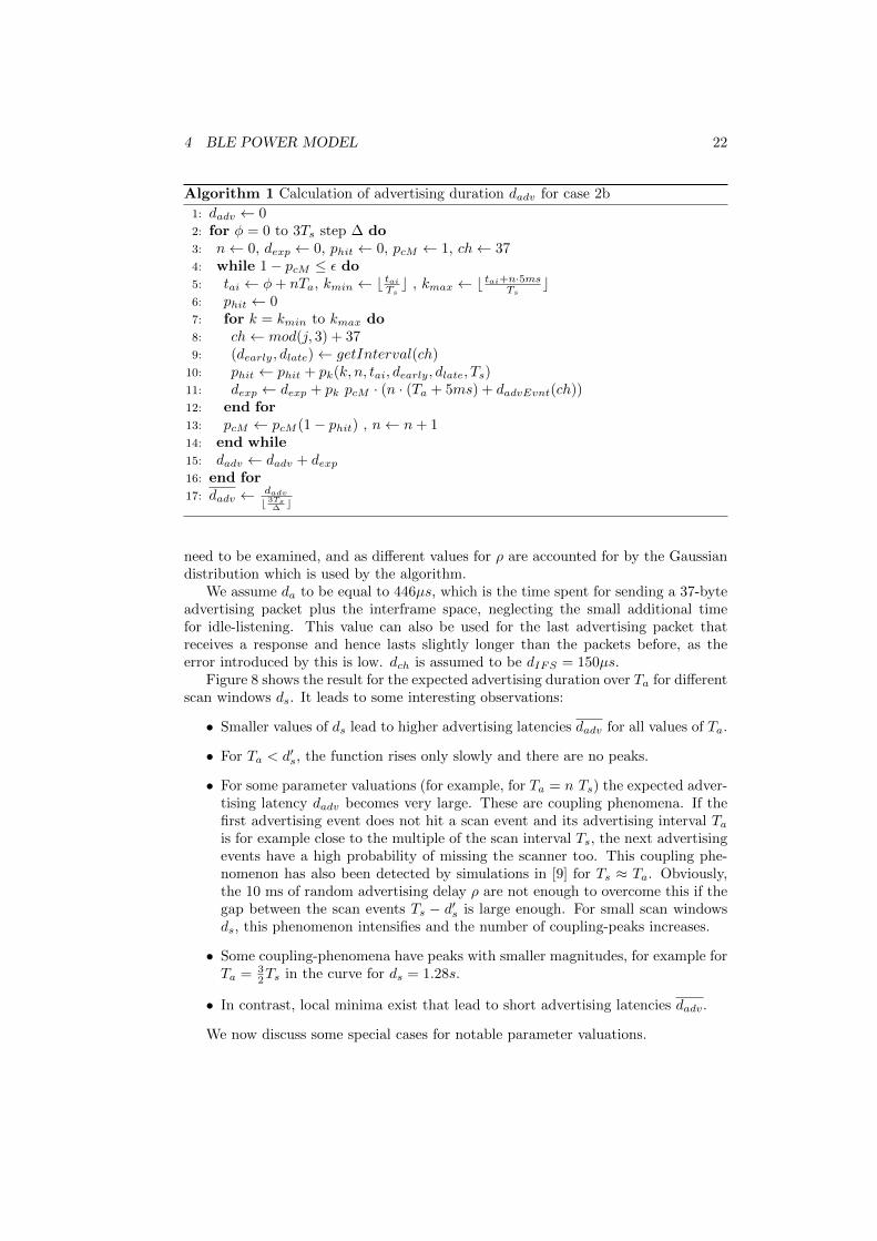
Algorithm 1 Calculation of advertising duration dadv for case 2b
1: dadv ← 02: for φ = 0 to 3Ts step ∆ do3: n← 0, dexp ← 0, phit ← 0, pcM ← 1, ch← 374: while 1− pcM ≤ ε do5: tai ← φ+ nTa, kmin ← b tai
Tsc , kmax ← b tai+n·5ms
Tsc
6: phit ← 07: for k = kmin to kmax do8: ch← mod(j, 3) + 379: (dearly, dlate)← getInterval(ch)
10: phit ← phit + pk(k, n, tai, dearly, dlate, Ts)11: dexp ← dexp + pk pcM · (n · (Ta + 5ms) + dadvEvnt(ch))12: end for13: pcM ← pcM (1− phit) , n← n+ 114: end while15: dadv ← dadv + dexp16: end for17: dadv ← dadv
b 3Ts∆ c
need to be examined, and as different values for ρ are accounted for by the Gaussiandistribution which is used by the algorithm.
We assume da to be equal to 446µs, which is the time spent for sending a 37-byteadvertising packet plus the interframe space, neglecting the small additional timefor idle-listening. This value can also be used for the last advertising packet thatreceives a response and hence lasts slightly longer than the packets before, as theerror introduced by this is low. dch is assumed to be dIFS = 150µs.
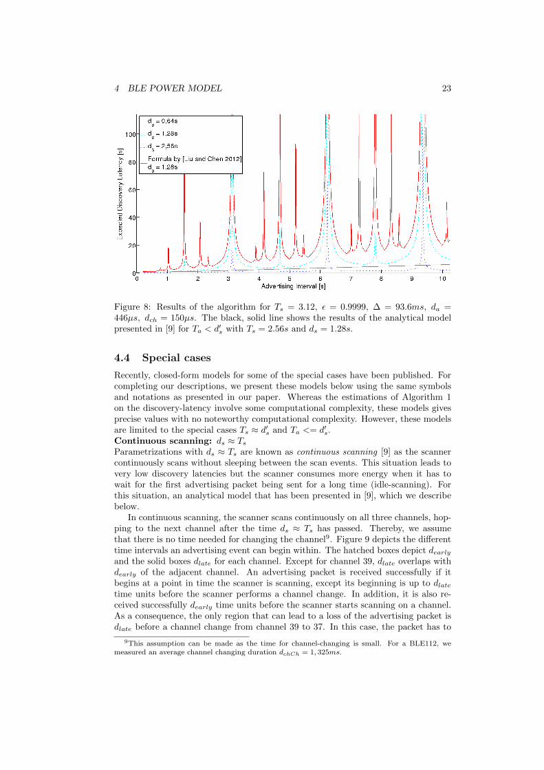
Figure 8 shows the result for the expected advertising duration over Ta for differentscan windows ds. It leads to some interesting observations:
• Smaller values of ds lead to higher advertising latencies dadv for all values of Ta.
• For Ta < d′s, the function rises only slowly and there are no peaks.
• For some parameter valuations (for example, for Ta = n Ts) the expected adver-tising latency dadv becomes very large. These are coupling phenomena. If thefirst advertising event does not hit a scan event and its advertising interval Tais for example close to the multiple of the scan interval Ts, the next advertisingevents have a high probability of missing the scanner too. This coupling phe-nomenon has also been detected by simulations in [9] for Ts ≈ Ta. Obviously,the 10 ms of random advertising delay ρ are not enough to overcome this if thegap between the scan events Ts − d′s is large enough. For small scan windowsds, this phenomenon intensifies and the number of coupling-peaks increases.
• Some coupling-phenomena have peaks with smaller magnitudes, for example forTa = 3
2Ts in the curve for ds = 1.28s.
• In contrast, local minima exist that lead to short advertising latencies dadv.
We now discuss some special cases for notable parameter valuations.
4 BLE POWER MODEL 23
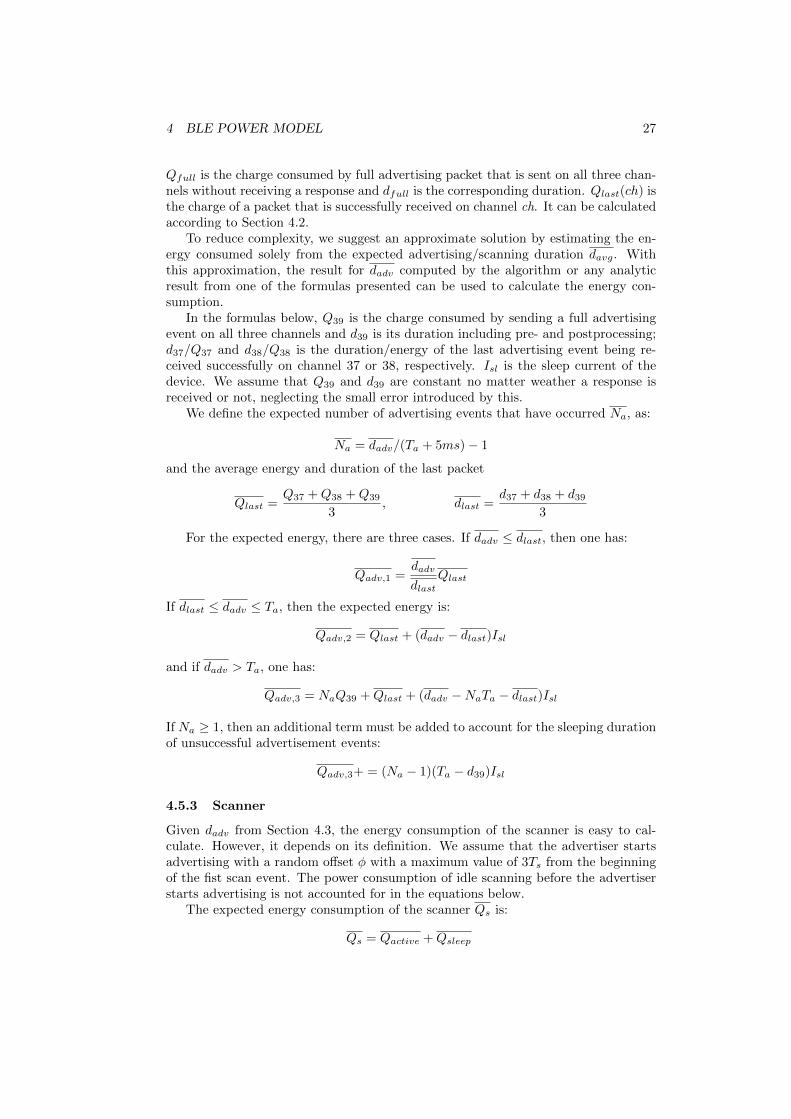
Figure 8: Results of the algorithm for Ts = 3.12, ε = 0.9999, ∆ = 93.6ms, da =446µs, dch = 150µs. The black, solid line shows the results of the analytical modelpresented in [9] for Ta < d′s with Ts = 2.56s and ds = 1.28s.
4.4 Special cases
Recently, closed-form models for some of the special cases have been published. Forcompleting our descriptions, we present these models below using the same symbolsand notations as presented in our paper. Whereas the estimations of Algorithm 1on the discovery-latency involve some computational complexity, these models givesprecise values with no noteworthy computational complexity. However, these modelsare limited to the special cases Ts ≈ d′s and Ta <= d′s.Continuous scanning: ds ≈ TsParametrizations with ds ≈ Ts are known as continuous scanning [9] as the scannercontinuously scans without sleeping between the scan events. This situation leads tovery low discovery latencies but the scanner consumes more energy when it has towait for the first advertising packet being sent for a long time (idle-scanning). Forthis situation, an analytical model that has been presented in [9], which we describebelow.
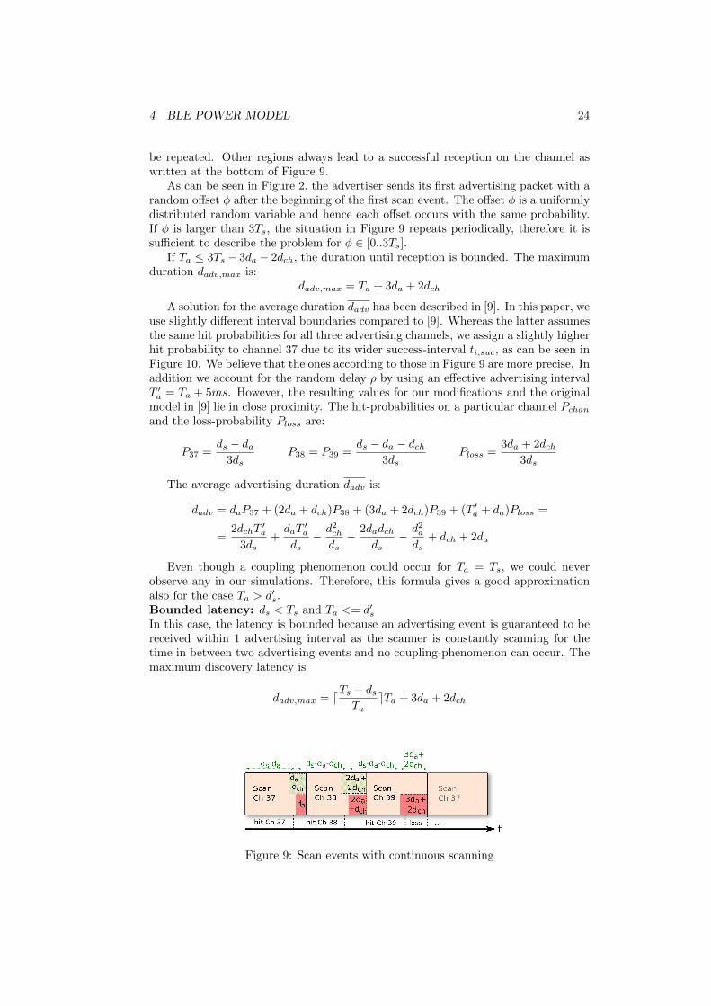
In continuous scanning, the scanner scans continuously on all three channels, hop-ping to the next channel after the time ds ≈ Ts has passed. Thereby, we assumethat there is no time needed for changing the channel9. Figure 9 depicts the differenttime intervals an advertising event can begin within. The hatched boxes depict dearlyand the solid boxes dlate for each channel. Except for channel 39, dlate overlaps withdearly of the adjacent channel. An advertising packet is received successfully if itbegins at a point in time the scanner is scanning, except its beginning is up to dlatetime units before the scanner performs a channel change. In addition, it is also re-ceived successfully dearly time units before the scanner starts scanning on a channel.As a consequence, the only region that can lead to a loss of the advertising packet isdlate before a channel change from channel 39 to 37. In this case, the packet has to
9This assumption can be made as the time for channel-changing is small. For a BLE112, wemeasured an average channel changing duration dchCh = 1, 325ms.
4 BLE POWER MODEL 24
be repeated. Other regions always lead to a successful reception on the channel aswritten at the bottom of Figure 9.
As can be seen in Figure 2, the advertiser sends its first advertising packet with arandom offset φ after the beginning of the first scan event. The offset φ is a uniformlydistributed random variable and hence each offset occurs with the same probability.If φ is larger than 3Ts, the situation in Figure 9 repeats periodically, therefore it issufficient to describe the problem for φ ∈ [0..3Ts].
If Ta ≤ 3Ts − 3da − 2dch, the duration until reception is bounded. The maximumduration dadv,max is:
dadv,max = Ta + 3da + 2dch
A solution for the average duration dadv has been described in [9]. In this paper, weuse slightly different interval boundaries compared to [9]. Whereas the latter assumesthe same hit probabilities for all three advertising channels, we assign a slightly higherhit probability to channel 37 due to its wider success-interval ti,suc, as can be seen inFigure 10. We believe that the ones according to those in Figure 9 are more precise. Inaddition we account for the random delay ρ by using an effective advertising intervalT ′a = Ta + 5ms. However, the resulting values for our modifications and the originalmodel in [9] lie in close proximity. The hit-probabilities on a particular channel Pchanand the loss-probability Ploss are:
P37 =ds − da
3dsP38 = P39 =
ds − da − dch3ds
Ploss =3da + 2dch
3ds
The average advertising duration dadv is:
dadv = daP37 + (2da + dch)P38 + (3da + 2dch)P39 + (T ′a + da)Ploss =
=2dchT
′a
3ds+daT
′a
ds− d2
ch
ds− 2dadch
ds− d2
a
ds+ dch + 2da
Even though a coupling phenomenon could occur for Ta = Ts, we could neverobserve any in our simulations. Therefore, this formula gives a good approximationalso for the case Ta > d′s.Bounded latency: ds < Ts and Ta <= d′sIn this case, the latency is bounded because an advertising event is guaranteed to bereceived within 1 advertising interval as the scanner is constantly scanning for thetime in between two advertising events and no coupling-phenomenon can occur. Themaximum discovery latency is
dadv,max = dTs − dsTa
eTa + 3da + 2dch
Figure 9: Scan events with continuous scanning
4 BLE POWER MODEL 25
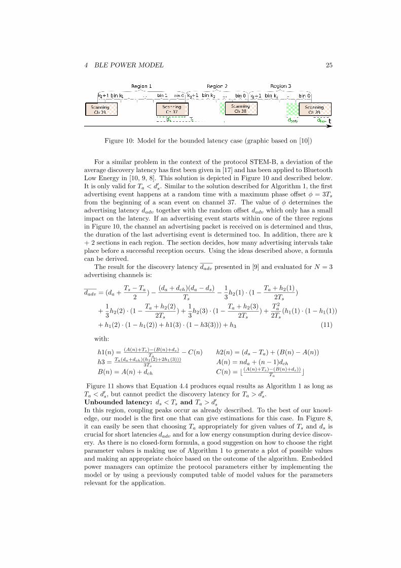
Figure 10: Model for the bounded latency case (graphic based on [10])
For a similar problem in the context of the protocol STEM-B, a deviation of theaverage discovery latency has first been given in [17] and has been applied to BluetoothLow Energy in [10, 9, 8]. This solution is depicted in Figure 10 and described below.It is only valid for Ta < d′s. Similar to the solution described for Algorithm 1, the firstadvertising event happens at a random time with a maximum phase offset φ = 3Tsfrom the beginning of a scan event on channel 37. The value of φ determines theadvertising latency dadv together with the random offset dadv which only has a smallimpact on the latency. If an advertising event starts within one of the three regionsin Figure 10, the channel an advertising packet is received on is determined and thus,the duration of the last advertising event is determined too. In addition, there are k+ 2 sections in each region. The section decides, how many advertising intervals takeplace before a successful reception occurs. Using the ideas described above, a formulacan be derived.
The result for the discovery latency dadv presented in [9] and evaluated for N = 3advertising channels is:
dadv = (da +Ts − Ta
2)− (da + dch)(da − ds)
Ts− 1
3h2(1) · (1− Ta + h2(1)
2Ts)
+1
3h2(2) · (1− Ta + h2(2)
2Ts) +
1
3h2(3) · (1− Ta + h2(3)
2Ts) +
T 2a
2Ts(h1(1) · (1− h1(1))
+ h1(2) · (1− h1(2)) + h1(3) · (1− h3(3))) + h3 (11)
with:
h1(n) = (A(n)+Ts)−(B(n)+ds)Ta
− C(n) h2(n) = (ds − Ta) + (B(n)−A(n))
h3 = Ta(da+dch)(h1(2)+2h1(3)))3Ts
A(n) = nda + (n− 1)dch
B(n) = A(n) + dch C(n) = b (A(n)+Ts)−(B(n)+ds))Ta
c
Figure 11 shows that Equation 4.4 produces equal results as Algorithm 1 as long asTa < d′s, but cannot predict the discovery latency for Ta > d′s.Unbounded latency: ds < Ts and Ta > d′sIn this region, coupling peaks occur as already described. To the best of our knowl-edge, our model is the first one that can give estimations for this case. In Figure 8,it can easily be seen that choosing Ta appropriately for given values of Ts and ds iscrucial for short latencies dadv and for a low energy consumption during device discov-ery. As there is no closed-form formula, a good suggestion on how to choose the rightparameter values is making use of Algorithm 1 to generate a plot of possible valuesand making an appropriate choice based on the outcome of the algorithm. Embeddedpower managers can optimize the protocol parameters either by implementing themodel or by using a previously computed table of model values for the parametersrelevant for the application.
4 BLE POWER MODEL 26
4.5 Computing the number of events
After having presented a model for each type of event that can occur and a modelfor the expected advertising latency dadv, we combine both to obtain the energyconsumption for device discovery. Therefore, we calculate the number of events thattake place within dadv to obtain the energy consumption of the advertiser and thescanner. For the connected mode, this problem is much simpler as the repetitionperiod of the connection events is known and the number of events that occur withina given amount of time can be easily calculated.
4.5.1 Connected Mode
For a master, the number of connection events Nc,ma in a given amount of time Tg is
Nc,ma = bTgTcc
For the slave, the number of connection events Nc,sl is different as it may skip someevents due to the slave latency parameter Nsl. With an average number of Nsl skippedevents, the energy-consumption for the slave is
Nc,sl = b Tg
NslTcc
The overall charge consumption of the master or the slave is the sum of the eventenergies and the sleeping energy:
Qcon,Ma/Sl =
Nc∑n=1
Qevent(n) + (Tg −Nc∑n=1
devent(n))Isl (12)
In Equation 4.5.1, Nc can be set to the number of connection events for the master(Nc = Nc,ma) or for the slave (Nc = Nc,sl). Qevent can be calculated according toSection 4.2. Isl is the sleep current of the device and devent(n) the duration of eventn.
4.5.2 Advertiser
The energy consumption of one advertising event QadvEvent can be modeled as de-scribed in Section 4.2. For calculating the expected energy consumption Qadv fordevice discovery of the advertiser, it must be taken into account that not all adver-tising events are identical. Events that are successfully received might be shorterthan the other events as packets on different advertising channels are skipped after asuccessful reception, and the rx -phase takes longer due to receiving the response.
The exact calculation can only be done within Algorithm 1 or, in cases thereis an analytical formula available, by modifying this formula. In the case of non-continuous scanning with Ta < w′s, this has been done in [8]. In general, Algorithm 1can easily be extended for an estimation of the advertiser’s energy. With Qadv beingthe expected energy of the advertiser, one could add the following assignment afterLine 11 of Algorithm 1:
Qadv ← Qadv + pk pcM ((n− 1)(Qfull + (Ta − dfull)Isl) +Qlast(ch))
4 BLE POWER MODEL 27
Qfull is the charge consumed by full advertising packet that is sent on all three chan-nels without receiving a response and dfull is the corresponding duration. Qlast(ch) isthe charge of a packet that is successfully received on channel ch. It can be calculatedaccording to Section 4.2.
To reduce complexity, we suggest an approximate solution by estimating the en-ergy consumed solely from the expected advertising/scanning duration davg. Withthis approximation, the result for dadv computed by the algorithm or any analyticresult from one of the formulas presented can be used to calculate the energy con-sumption.
In the formulas below, Q39 is the charge consumed by sending a full advertisingevent on all three channels and d39 is its duration including pre- and postprocessing;d37/Q37 and d38/Q38 is the duration/energy of the last advertising event being re-ceived successfully on channel 37 or 38, respectively. Isl is the sleep current of thedevice. We assume that Q39 and d39 are constant no matter weather a response isreceived or not, neglecting the small error introduced by this.
We define the expected number of advertising events that have occurred Na, as:
Na = dadv/(Ta + 5ms)− 1
and the average energy and duration of the last packet
Qlast =Q37 +Q38 +Q39
3, dlast =
d37 + d38 + d39
3
For the expected energy, there are three cases. If dadv ≤ dlast, then one has:
Qadv,1 =dadv
dlastQlast
If dlast ≤ dadv ≤ Ta, then the expected energy is:
Qadv,2 = Qlast + (dadv − dlast)Isl
and if dadv > Ta, one has:
Qadv,3 = NaQ39 +Qlast + (dadv −NaTa − dlast)Isl
If Na ≥ 1, then an additional term must be added to account for the sleeping durationof unsuccessful advertisement events:
Qadv,3+ = (Na − 1)(Ta − d39)Isl
4.5.3 Scanner
Given dadv from Section 4.3, the energy consumption of the scanner is easy to cal-culate. However, it depends on its definition. We assume that the advertiser startsadvertising with a random offset φ with a maximum value of 3Ts from the beginningof the fist scan event. The power consumption of idle scanning before the advertiserstarts advertising is not accounted for in the equations below.
The expected energy consumption of the scanner Qs is:
Qs = Qactive +Qsleep
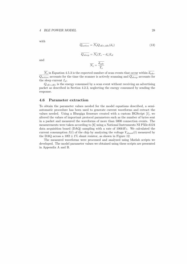
4 BLE POWER MODEL 28
withQactive = NsQsEv,idle(ds) (13)
Qsleep = Ns(Ts − ds)Island
Ns =dadvTs
Ns in Equation 4.5.3 is the expected number of scan events that occur within dadv.Qactive accounts for the time the scanner is actively scanning and Qsleep accounts forthe sleep current Isl.
QsEv,idle is the energy consumed by a scan event without receiving an advertisingpacket as described in Section 4.2.2, neglecting the energy consumed by sending theresponse.
4.6 Parameter extraction
To obtain the parameter values needed for the model equations described, a semi-automatic procedure has been used to generate current waveforms and extract thevalues needed. Using a Bluegiga firmware created with a custom BGScript [1], wealtered the values of important protocol parameters such as the number of bytes sentin a packet and measured the waveforms of more than 5000 connection events. Themeasurements were taken according to [6] using a National Instruments NI PXIe-6124data acquisition board (DAQ) sampling with a rate of 100kHz. We calculated thecurrent consumption I(t) of the chip by analyzing the voltage Vshunt(t) measured bythe DAQ across a 10Ω± 1% shunt resistor, as shown in Figure 12.
The measured waveforms were processed and analyzed using Matlab scripts wedeveloped. The model parameter values we obtained using these scripts are presentedin Appendix A and B.
4 BLE POWER MODEL 29
Figure 11: Model from Equation 4.4 compared to result from Algorithm 1 (Ts =3.12s, ∆ = 93.6ms, da = 446µs, dch = 150µs)
Figure 12: Measurement Setup
5 VERIFICATION OF THE MODEL 30
5 Verification of the model
In this section, we discuss the validity of our proposed model. Towards this, weconducted measurements both in the non-connected and in the connected mode andcompare the results with the modeled data. The only previous comparative mea-surements of such a model with real-world measurements or simulations have beenpresented in [8],[10], [9] for device-discovery with Ta < ds. In this paper, the discov-ery latency in the advertising-/scanning mode has been modeled and compared withmeasured data also for Ta > ds. For the connected mode, we measured the currentconsumption of a BLE112 module for a given scenario and compared it to the modeledvalues. The results show that modeled and measured data lie in close proximity.
5.1 Connected mode
To compare the modeled and the measured energy consumption in the connectedmode, we set up a test scenario. Two devices exchange data using a connectioninterval Tc of 100ms. One device sends data with an attribute-write request, theother node acknowledges the data received. We did this comparison for both, amaster and a slave sending the payload. The payload sent varies from 1 to 20 bytes,the number of packets sent per event is one per direction. The number of total bytesreceived in a response is either 10 or 15, depending on the event. The sequence ofconnection events in our scenario is as follows:
• Send a byte with a payload sweeping between 0 and 20 bytes with 17 bytesoverhead10 and receive an empty polling packet with 10 bytes total length.
• Send an empty polling packet with 10 bytes length and wait for the acknowl-edgement packet with 15 bytes length.
The model uses parameter values according to the tables in Appendix A. As thedevice showed an unexpectedly long duration of the first rx -phase of each connectionevent when acting as a slave, we did not use the value of dprerx from the table, butused the effective duration of dprerx = 388us11 for the slave.
To achieve a hight accuracy, we scheduled the preparation of the attribute-writerequests in a task that is run periodically on the BLE module by a separate timer.Consequently, it does not run within the pre- and postprocessing phase of an event.The current waveforms generated by this task were filtered out by a matlab script. Inaddition, we made sure the BLE device did not send anything other than the packetswe took into account in our model, such as a connection parameter update, duringthe time we were measuring. In our measurements, even though we used high-qualitymeasurement equipment, the bias current of the measurement device was larger thanthe sleep current of the BLE device. Therefore, in average, its measured value wasslightly negative. A Matlab-script detected the time when each connection eventoccurred in the measured current waveform and triggered the model to compute thecharge consumed for the same event at the same point in the simulated time.
Figure 13 shows the result of the experiments described. The curves depict theenergy-consumption over time for a master and a slave, both computed with our
10Sending a zero-byte-packet generates an empty polling packet having a total length of 10 bytes.11This value has been calculated based on our experiments for the values presented in Appendix
A and is valid for a BLE112 device for the first rx -phase of a connection event of a slave. We did notfind any dependence of this value on the connection interval. A measurement with a CC2540-devicewith TI’s BLE stack did not show such a significant abnormality.
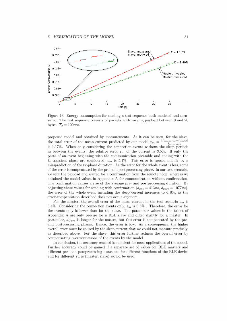
5 VERIFICATION OF THE MODEL 31
Figure 13: Energy consumption for sending a test sequence both modeled and mea-sured. The test sequence consists of packets with varying payload between 0 and 20bytes. Tc = 100ms.
proposed model and obtained by measurements. As it can be seen, for the slave,
the total error of the mean current predicted by our model εm = |Imeasured−Imodel|Imeasured
is 1.17%. When only considering the connection-events without the sleep periodsin between the events, the relative error εm of the current is 3.5%. If only theparts of an event beginning with the communication preamble and ending with thetx -transient phase are considered, εm is 5.1%. This error is caused mainly by amissprediction of the rx-phase duration. As the error for the whole event is less, someof the error is compensated by the pre- and postprocessing phase. In our test-scenario,we sent the payload and waited for a confirmation from the remote node, whereas weobtained the model-values in Appendix A for communication without confirmation.The confirmation causes a rise of the average pre- and postprocessing duration. Byadjusting these values for sending with confirmation (dpre = 413µs, dpost = 1077µs),the error of the whole event including the sleep current increases to 6, 0%, as theerror-compensation described does not occur anymore.
For the master, the overall error of the mean current in the test scenario εm is3.4%. Considering the connection events only, εm is 0.6% . Therefore, the error forthe events only is lower than for the slave. The parameter values in the tables ofAppendix A are only precise for a BLE slave and differ slightly for a master. Inparticular, dCpre is longer for the master, but this error is compensated by the pre-and postprocessing phases. Hence, the error is low. As a consequence, the higheroverall error must be caused by the sleep current that we could not measure precisely,as described above. For the slave, this error further reduces the overall error bycompensating overestimations of the events by the model.
In conclusion, the accuracy reached is sufficient for most applications of the model.Further accuracy could be gained if a separate set of values for BLE masters anddifferent pre- and postprocessing durations for different functions of the BLE deviceand for different rules (master, slave) would be used.

5 VERIFICATION OF THE MODEL 32
Figure 14: Measured discovery latency compared to modeled values. Model param-eters: Ts = 2.56s, ds = 1.28s, εm = 0.9999, ∆ = 76.8ms, , tmax = 1000s (modelaborted for times above), da = 446µs, dch = 150µs.
5.2 Advertising/Scanning
For verifying our algorithm, we measured the mean discovery latency dadv and com-pared these results with results from our model as shown in Figure 14.
The dashed curve shows the computed advertising latency dadv for different ad-vertising intervals Ta. In addition to this curve which has been obtained by usingAlgorithm 1, each cross in the figure shows the mean value of 100 real-world measure-ments that have been repeated with the same parameter values. These measurementshave been performed as follows. Two BLED112-modules have been connected to a PCwith the following configuration. One module is scanning continuously with fixed pa-rameters. As soon as a scan response is received, the process controlling this modulesends the time of reception to another process controlling the second module. Inter-process communication is handled by Unix-Domain-Sockets. The process controllingthe second module starts the advertising procedure at a random point in time between0s and 3Ts and calculates the duration between the start of the advertising and thefirst reception at the scanner. After having repeated this 100 times for one advertis-ing interval, the average duration is computed and Ta is increased by 63.5ms. Thissequence is repeated until the maximum advertising interval is reached. Advertisingintervals that lie within a coupling peak according to the model have been skipped asthe measurement would take a very high amount of time. As it can be seen in Figure14, results from the measurements and results obtained from the model lie in closeproximity. In addition to real-world measurements, we compared results from themodel to results from discrete event simulations which also lay in close proximity. Asthe issue is similar to connected mode and comparative measurements for advertising(for Ta < d′s) have already been done in [8], we did not measure the device discoveryenergy.
6 RESULTS AND CONCLUSION 33
6 Results and Conclusion
6.1 Sensitivity Analysis
Some of the durations and current magnitudes of the phases in a connection eventvary randomly. For example, the duration of the post-processing phase dpost is subjectto strong random variations. Another varying value is the current magnitude inthe transmission phase, Itx. If the standard deviations and the minimal/maximalvalues for the varying parameters are known, the impact of these variations on theoverall current consumption within one connection interval can be determined. This isimportant for getting an estimation for the maximum short-time current consumption.
In this section, we analyze the impact of variations of dpost and Itx on the energyconsumption in one connection interval. Thereby, we assume that the device is sleep-ing whenever there is no connection event taking place. For other parameters, thissensitivity analysis can be done similarly.Given a phase ph, dmin ≤ dph ≤ dmax, Imin ≤ Iph ≤ Imax, the sensitivity S on theduration dph or current Iph of a phase is:
S(dph) =∆Qtotal∆dph
S(Iph) =∆Qtotal
∆Iph
Qtotal is the total charge consumed within one connection interval, as calculated inEquation 4.5.1 with Nc = 1. All parameter values can be assumed to be independentfrom each other. Therefore, the sensitivity analysis can be done by accounting for thevariations of each parameter individually, assuming that all other parameters havefixed values. With Qsl (Isl) being the charge consumed (current drawn by sleeping),the sensitivity Sdph can be written as:
S(dph) =∆Qph∆dph
+∆Qsl∆dph
=Qph(dmax)−Qph(dmin)− (dmax − dmin)Isl
(dmax − dmin)
The sensitivity on the current Iph consumed during a phase ph is
S(Iph) =∆Qph∆Iph
=Qph(Imax)−Qph(Imin)
Imax − Imin
By assuming that the current Iph and the duration dph of a phase are independentfrom each other, one can further simplify:
S(Iph) = dph, S(dph) = Iph − Isl
In case of the duration of the post-processing phase dpost, which is the para-meter having the strongest variations in our measurements, the change in energy-consumption of a connection interval is (using S(dpost) = Ipost − Isl = 8.0mA,∆dpost = 0.5ms, Qtotal = 25µC):
∆Qtotal(dpost) = ∆dpost · S(dpost) = 0.5ms · 8mA = 4.0µC
The relative change ∆Qtotal
Qtotalis 16%. This means, due to variations in the post-
processing phase, the energy consumption of a whole connection event might varyby 16%.

6 RESULTS AND CONCLUSION 34
The relative change in the energy consumption of a connection interval causedby variations in the transmission current Itx is (using S(Itx) = dtx · Nseq = 350µs,∆Itx = 10.0mA, Qtotal = 29µC):
∆QtotalQtotal
=10mA · 350µs
29µC= 12%
6.2 Using the model
With this paper, an implementation of our proposed energy model has been madeavailable [7]. It is written as a C-library that provides easy-to-use functions for es-timating the energy consumption of a BLE device and comes with a complete docu-mentation in Doxygen format. It has a small resource demand and does not rely onany external code except some standard libraries. Therefore, it can easily be portedto embedded platforms. The usage of the library is intuitive and illustrated withmany examples. For example, to calculate the charge-consumption of one connectioninterval of 10 ms with 5 pairs of packets per event, with 10 bytes received and 20 bytessent per packet and with 3dBm transmission power, the following code example canbe used.
#include "ble_model.h"
int main()
double charge;
charge = ble_e_model_c_getChargeConnectionIntervalSamePayload(0,0.1,5,10,20,3);
return 0;
6.3 Designer Guidelines
In this section, we present possible uses of our model, leading to guidelines for system-designers on optimizing their parameter values for power consumption.
6.3.1 Advertising/Scanning
Figure 15 shows the expected charge consumed by the advertiser and the scanner for differentscan windows ds. The solid lines depict the charges calculated directly within Algorithm1, whereas the dashed lines that overlap with the solid lines depcit the result using theFormulas 4.5.2, 4.5.2, 4.5.2 and 4.5.3. As can be seen, the estimates given by these formulasdo not differ significantly from the more exact curves that have been calculated directly byAlgorithm 1. As the formulas define a relation between dadv and the charge consumed, agood estimation for the energy consumption of the advertiser and scanner can be made ifdadv is given.
Figure 15 reveals some interesting results. First, the energy consumption of the scanneris significantly higher than the energy consumption of the advertiser for all parameter valuesexamined. Second, increasing the advertising interval does not increase the energy muchif Ta is not chosen to be within one of the peaks. However, a high Ta reduces the energyconsumption of idle-advertising significantly. This makes the mode Ta > d′s a good choice forneighbor discovery of devices that are expected to spend a long time in idle-scanning/idle-advertising because their remote nodes seldom come into range and if a higher discovery-latency is uncritical. Another interesting outcome is that for the scanner, the scan windowdoes not influence its energy consumption much if Ta is small. As Ta increases, biggerscan-windows are better in terms of energy consumed by the scanner.
From the model results, we propose the following choices to energy-optimize neighbordiscovery procedures:
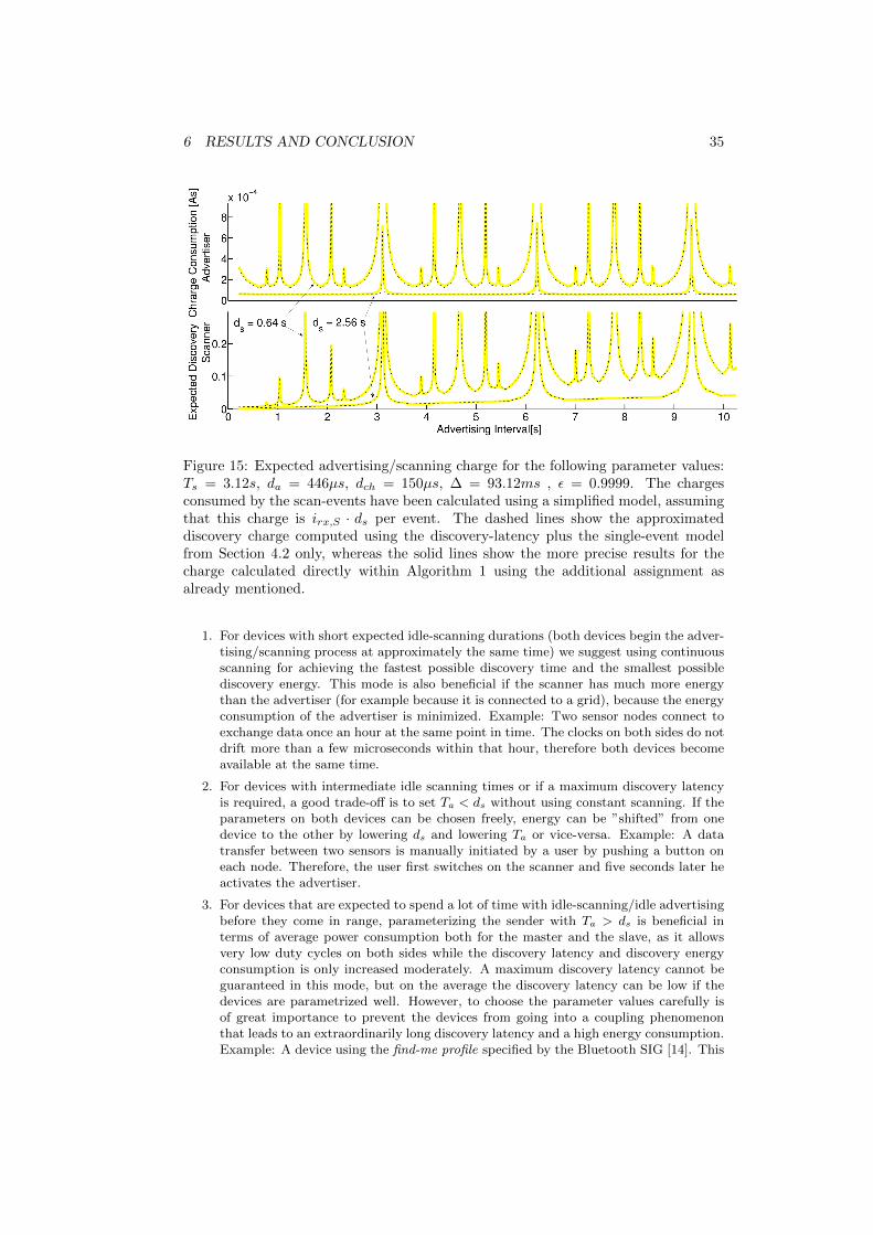
6 RESULTS AND CONCLUSION 35
Figure 15: Expected advertising/scanning charge for the following parameter values:Ts = 3.12s, da = 446µs, dch = 150µs, ∆ = 93.12ms , ε = 0.9999. The chargesconsumed by the scan-events have been calculated using a simplified model, assumingthat this charge is irx,S · ds per event. The dashed lines show the approximateddiscovery charge computed using the discovery-latency plus the single-event modelfrom Section 4.2 only, whereas the solid lines show the more precise results for thecharge calculated directly within Algorithm 1 using the additional assignment asalready mentioned.
1. For devices with short expected idle-scanning durations (both devices begin the adver-tising/scanning process at approximately the same time) we suggest using continuousscanning for achieving the fastest possible discovery time and the smallest possiblediscovery energy. This mode is also beneficial if the scanner has much more energythan the advertiser (for example because it is connected to a grid), because the energyconsumption of the advertiser is minimized. Example: Two sensor nodes connect toexchange data once an hour at the same point in time. The clocks on both sides do notdrift more than a few microseconds within that hour, therefore both devices becomeavailable at the same time.
2. For devices with intermediate idle scanning times or if a maximum discovery latencyis required, a good trade-off is to set Ta < ds without using constant scanning. If theparameters on both devices can be chosen freely, energy can be ”shifted” from onedevice to the other by lowering ds and lowering Ta or vice-versa. Example: A datatransfer between two sensors is manually initiated by a user by pushing a button oneach node. Therefore, the user first switches on the scanner and five seconds later heactivates the advertiser.
3. For devices that are expected to spend a lot of time with idle-scanning/idle advertisingbefore they come in range, parameterizing the sender with Ta > ds is beneficial interms of average power consumption both for the master and the slave, as it allowsvery low duty cycles on both sides while the discovery latency and discovery energyconsumption is only increased moderately. A maximum discovery latency cannot beguaranteed in this mode, but on the average the discovery latency can be low if thedevices are parametrized well. However, to choose the parameter values carefully isof great importance to prevent the devices from going into a coupling phenomenonthat leads to an extraordinarily long discovery latency and a high energy consumption.Example: A device using the find-me profile specified by the Bluetooth SIG [14]. This

6 RESULTS AND CONCLUSION 36
might be a keyfob that is lost and therefore is being looked for by another device likea smartphone. We consider the case where the keyfob is not in range because it is inthe pocket of a person in another room. For instance, 30 minutes pass until the personenters the room and the advertiser meets the scanner. In the find-me profile specifiedby Bluetooth SIG[14], a parametrization with Ta > ds is used after 30ms of lowerduty-cycle scanning. Ts is recommended to be 2.56s with ds = 11.25ms (”Option2”). In this profile, the advertising interval after 30ms of advertising is suggested tobe between 1s and 2.5s [14]. According to our model, Ts = Ta = 2.5s would leadto high discovery energies and mean latencies as high as 560s - as this constellationleads to a coupling phenomenon. Therefore, we propose a different value selection andrecommend that further versions of the profile forbid such parameter combinations.
To avoid this situation, we propose to plot dadv for the range of parameters that areconsidered and choose an appropriate local minimum.
6.3.2 Connected mode
Figure 16: Current consumption for different payload throughputs (goodput) usingdifferent payload sizes per event for a slave. The protocol overhead is 17 bytes perpacket.
For the connected mode, a parametrization needs to be chosen that optimizes the energyconsumption for given constraints on minimum throughput and maximum latency.
Figure 16 shows the mean current of a BLE device with different amounts of payloadbytes per connection event. Every packet sent contains 17 bytes protocol overhead and amaximum of 20 bytes payload. If there is more payload in an event than 20 bytes, twoor more packets can be transmitted in one event. Given a fixed amount of payload perevent, different throughputs of the payload (goodputs) can be achieved by modifying theconnection interval. In addition to the goodput-energy curves, different energy-efficienciesper byte are shown as diagonal lines in the figure. As can be seen, the transmission takesplace with different efficiencies η = bytes
chargefor different parameter values. A parametrization
drawing a higher current consumption can have a better efficiency per byte payload thanothers drawing a lower current. For example, the efficiency of the point with the smallestcurrent and smallest goodput at the lower left of the figure is by far less than achieving thesame throughput with 16 bytes per event. Another fact that can be observed is that forany of the curves with a fixed payload per event, the increase of the goodput leads to a riseof the efficiency but at the same time to an increased current consumption. In conclusion,
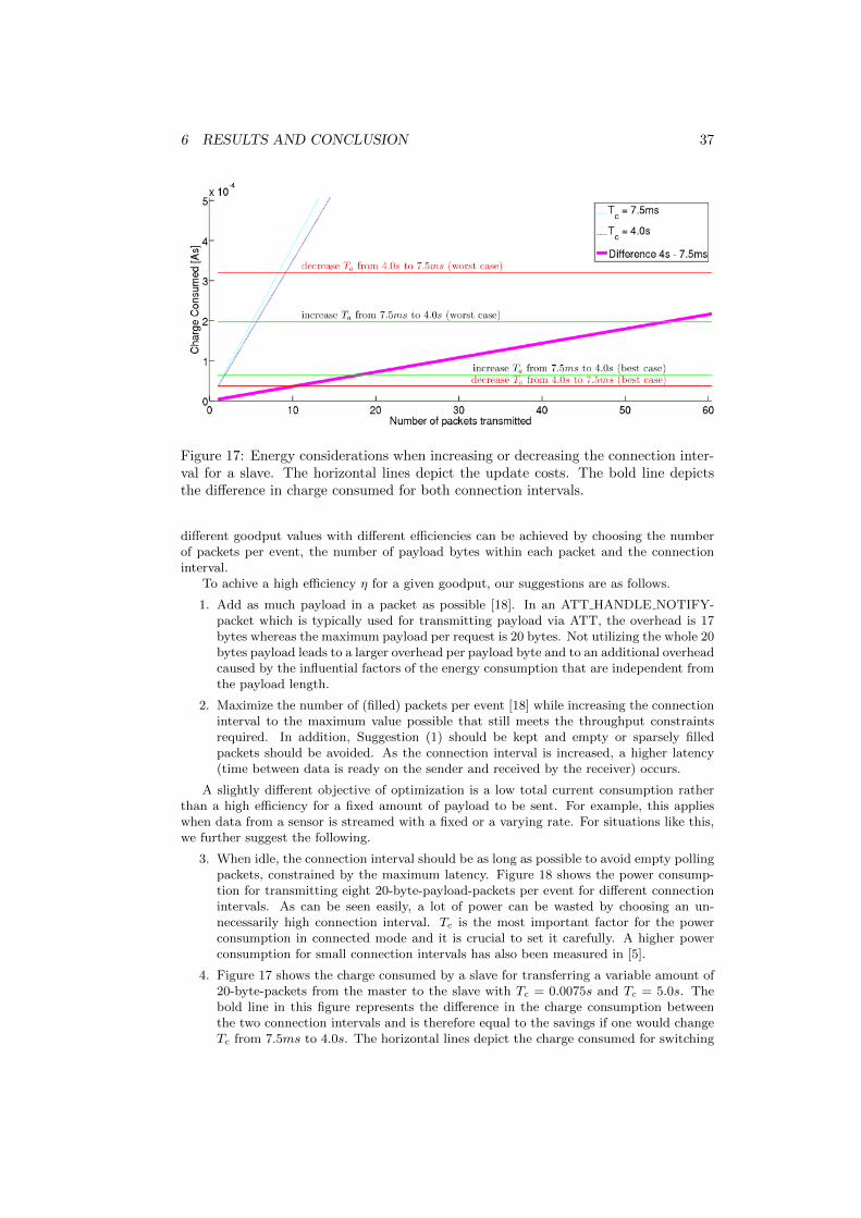
6 RESULTS AND CONCLUSION 37
Figure 17: Energy considerations when increasing or decreasing the connection inter-val for a slave. The horizontal lines depict the update costs. The bold line depictsthe difference in charge consumed for both connection intervals.
different goodput values with different efficiencies can be achieved by choosing the numberof packets per event, the number of payload bytes within each packet and the connectioninterval.
To achive a high efficiency η for a given goodput, our suggestions are as follows.
1. Add as much payload in a packet as possible [18]. In an ATT HANDLE NOTIFY-packet which is typically used for transmitting payload via ATT, the overhead is 17bytes whereas the maximum payload per request is 20 bytes. Not utilizing the whole 20bytes payload leads to a larger overhead per payload byte and to an additional overheadcaused by the influential factors of the energy consumption that are independent fromthe payload length.
2. Maximize the number of (filled) packets per event [18] while increasing the connectioninterval to the maximum value possible that still meets the throughput constraintsrequired. In addition, Suggestion (1) should be kept and empty or sparsely filledpackets should be avoided. As the connection interval is increased, a higher latency(time between data is ready on the sender and received by the receiver) occurs.
A slightly different objective of optimization is a low total current consumption ratherthan a high efficiency for a fixed amount of payload to be sent. For example, this applieswhen data from a sensor is streamed with a fixed or a varying rate. For situations like this,we further suggest the following.
3. When idle, the connection interval should be as long as possible to avoid empty pollingpackets, constrained by the maximum latency. Figure 18 shows the power consump-tion for transmitting eight 20-byte-payload-packets per event for different connectionintervals. As can be seen easily, a lot of power can be wasted by choosing an un-necessarily high connection interval. Tc is the most important factor for the powerconsumption in connected mode and it is crucial to set it carefully. A higher powerconsumption for small connection intervals has also been measured in [5].
4. Figure 17 shows the charge consumed by a slave for transferring a variable amount of20-byte-packets from the master to the slave with Tc = 0.0075s and Tc = 5.0s. Thebold line in this figure represents the difference in the charge consumption betweenthe two connection intervals and is therefore equal to the savings if one would changeTc from 7.5ms to 4.0s. The horizontal lines depict the charge consumed for switching

6 RESULTS AND CONCLUSION 38
Figure 18: Current consumption for different connection intervals and tx -power levelsfor 8 packets per event with 20 bytes payload + 17 bytes overhead in each packet.The line for the slave shows the current the slave needs to receive the packets andrespond with an empty packet.
from Tc = 7.5ms to Tc = 4.0s and vice versa, according to the procedure describedin Section 4.2.3. As mentioned before, the energy consumption for this proceduredepends on parameter values chosen by the stack and a best case/worst case estimationof the energy consumption can be made. We now consider after how many connectionintervals increasing the Tc from 7.5ms to 4.0s pays of energetically. In this example,in the best case, increasing the connection interval is beneficial after approximately18 events. In the worst case, it is beneficial after approximately 55 events. The costfor switching back is also shown in the figure. The worst case charge for a connectionupdate is much higher than for the best case due to the long possible transmit windowdtw, but should occur very rarely as the master normally uses small transmit windowsizes and schedules the anchor point for the new interval reasonably. With theseresults, one should consider renegotiating the connection interval whenever there is achange in the throughput required. Our proposed model can be used to estimate if theexpected savings in the energy consumption with the new connection interval prevailsthe cost for updating the connection parameters.
5. Using slave latency instead of lowering the connection interval is not beneficial if thethroughput required by the slave is known, as the energy of the master rarely lowerswith higher slave latency because it cannot skip the connection events. However, thecurve in Figure 18 could be extended towards longer effective connection intervals forthe slave by using slave latency. Therefore, there is a trade-off between renegotiatingthe connection interval frequently and keeping the connection interval constant whileusing slave latency: The slave might set a long effective connection interval if it islikely that there is few data to be sent, or it might just skip some connection intervalsand save the power for renegotiation of the connection interval if the data rate is likelyto rise again. The latter will result in a higher energy consumption for the master as,opposed to the slave, it cannot skip any connection interval.
6. Figure 18 reveals that energy can be saved if the tx -power-level is adjusted to a valuethat is sufficient to transmit the data across the distance between sender and receiverwithout loss instead of sending with the maximum power. The curves for different tx -powers lie in close proximity. Whereas it is desirable to send with the lowest possiblepower the device and the application allows, the impact of this factor is much smaller

6 RESULTS AND CONCLUSION 39
than others such as the connection interval.
6.4 Limitations
This paper described methods for estimating the energy consumption of a BLE device.However, there are some limitations.
6.4.1 Exponential peaks in advertising/scanning
As we abort Algorithm 1 for all times dexp > dexp,max, we cannot model the center ofexponential peaks. In close vicinity of these peaks, we loose accuracy. As the model iscapable of predicting these peaks, the discovery-latencies and -energies in these peaks arenot of interest as no designer would choose such a parametrization. Only the exact valuesof those parameters that are not within these peaks matter.
6.4.2 Ambiguous model parameters in advertising/scanning
Within Algorithm 1, there are two parameters ε and ∆ that affect the quality of the modelresults. At the moment, we cannot provide a meta-model that gives an estimation of theerror depending on the quality parameters. Setting them unnecessarily high will lead to along runtime of the model algorithm. Until now, these values have to be chosen based on agood guess.
6.4.3 Repetated Broadcasting
We presented a model for the average advertising latency dadv. Therefore, we can modela pair of nodes discovering each other for connection establishment and we can model theaverage latency until reception if a device periodically sends data in non-connected mode andchanges the data after random amounts of time (for example when a sensed value changes).However, there is a case that cannot be modeled properly, yet: Consider the situation whereone node is scanning and the other node is broadcasting data repeatedly, without getting anacknowledgement when data is received. The same broadcast data is repeated with Ta untilnew data is ready. Now we can calculate the average latency dadv as described, which is theaverage duration until the first successful reception takes place. For the second reception,our scheme cannot be applied as the new offset φ is not uniformly distributed anymore. Itdepends on the first offset, on the number of advertising events that occurred and on the
accumulated sum of random advertising delaysn∑1
ρ.
6.4.4 Preprocessing/Postprocessing
The preprocessing and postprocessing durations vary from event to event. As it significantlycontributes to the overall power consumption, an exact model that is capable of predicting theactual values in each event would be preferable over current models that can only predictmean values. The details needed to model the processing durations precisely are hiddenwithin the firmwares of the BLE modules - it falls into the responsibility of the firmwaredevelopers to make this data available.
6.5 Concluding remarks
In this paper, a precise and comprehensive model of the BLE protocol was presented. Themodel parameter values for BLE112-devices were given. These model-parameters need tobe remeasured for other devices. The model has proven good accuracies - in a test-scenario,an error of the predicted current of less than 6% in connected mode was measured. Theaccuracy can be increased by using individual sets of model-parameters for different BLE
7 CREDITS 40
functions. The proposed model can be used for battery lifetime calculations, for predictionson worst case peak currents and for deriving power management strategies. With the resultspresented, power-management-algorithms for updating the connection parameters adaptivelyto the current situation can be developed.
Further research on an error estimation for the parameters ∆ and ε of Algorithm 1 seemsto be desirable for reducing the runtime of the algorithm. An open research topic is thereception probability in continuous broadcasting scenarios. In addition, refined models forthe pre- and postprocessing durations should be derived in the future for further increasingthe model’s accuracy.
Modeled results have been compared to measured ones for the connected mode and for theneighbor discovery latency. Further comparative measurements are required to determinethe accuracy of the model for scan events and for the connection establishment/updateprocedure model. However, as the models have been derived from real world measurements,the expected accuracies should be similar to the ones for the connected mode.
7 Credits
This work was partially supported by ”HE2mT - High-Level Development Methods forEnergy-Saving, Mobile Telemonitoring Systems”, a project funded by the Federal Min-istry of Education and Research of Germany. Author’s emails: kindt, yunge, diemer,[email protected] Author’s addresses: Lehrstuhl fur Realzeit-Computersysteme,Technische Universitat Munchen, Arcisstr. 21, 80333 Munchen, Germany. This paper is insubmission to a journal. If it is accepted, it will be updated such that a link to the publishedpaper and the DOI will be provided. This document contains the non-reviewed version ofthe authors.
References
[1] Bluegiga. Ble112 data sheet, 2011. Version 1.21,URL: www.bluetooth.org/tpg/RefNotes/BLE112_Datasheet1.pdf.
[2] A. Chattopadhyay. ”application note an097: Current savingsin cc254x using the tps62730, 2012. Revision SWRA365, URL:www.ti.com/lit/an/swra365b/swra365b.pdf.
[3] M.C. Ekstrom, M. Bergblomma, M. Linden, M. Bjorkman, and M. Ekstrom. A blue-tooth radio energy consumption model for low-duty-cycle applications. IEEE Transac-tions on Instrumentation and Measurement (TIM), 61(3):609–617, 2012.
[4] C. Gomez, I. Demirkol, and J. Paradells. Modeling the maximum throughput of blue-tooth low energy in an error-prone link. IEEE Communications Letters, 15(11):1187–1189, 2011.
[5] C. Gomez, J. Oller, and J. Paradells. Overview and evaluation of bluetooth low energy:An emerging low-power wireless technology. Sensors, 12(9):11734–11753, 2012.
[6] S. Kamath and J. Lindh. Application note an092: Measuring blue-tooth low energy power consumption, 2012. Revision SWRA347a, URL:http://www.ti.com/lit/an/swra347a/swra347a.pdf.
[7] P. Kindt, D. Yunge, R. Diemer, and S. Chakraborty. C-implementation of the ble en-ergy model. http://www.rcs.ei.tum.de/en/research/wireless-sensor-networks/
bleemod, 2014.
[8] J. Liu and C. Chen. Energy analysis of neighbor discovery in blue-tooth low energy networks. Technical report, 07/2012 2012. URL:research.nokia.com/files/public/TR-EnergyAnalysis-BLE.pdf.

A PARAMETER VALUES FOR BLE112 IN CONNECTED MODE 41
[9] J. Liu, C. Chen, and Y. Ma. Modeling and performance analysis of device discoveryin bluetooth low energy networks. In 2012 IEEE Global Communications Conference(GLOBECOM), 2012.
[10] J. Liu, C. Chen, and Y. Ma. Modeling neighbor discovery in bluetooth low energynetworks. IEEE Communications Letters, 16(9):1439–1441, 2012.
[11] E. Mackensen, M. Lai, and T.M. Wendt. Bluetooth low energy (ble) based wirelesssensors. In 2012 IEEE Sensors, 2012.
[12] E. Mackensen, M. Lai, and T.M. Wendt. Performance analysis of an bluetooth lowenergy sensor system. In 2012 IEEE 1st International Symposium on Wireless Systems(IDAACS-SWS), 2012.
[13] Bluetooth SIG. Specification of the bluetooth system 4.0, June 2010. Volume 0, availablevia bluetooth.org.
[14] Bluetooth SIG. Find me profile specificiation, June 2011. Revision V10r00, availablevia bluetooth.org.
[15] Texas Instruments. Smartrf packet sniffer user manual, 2010. Revision F, URL:www.ti.com/lit/pdf/swru187.
[16] Texas Instruments. Cc2540f128, cc2540f256: 2.4-ghz bluetooth low energysystem-on-chip, 2014. SWRS084E, Version revised in june 2013, URL:http://www.ti.com/lit/gpn/cc2540.
[17] C. Schurgers, V. Tsiatsis, S. Ganeriwal, and M. Srivastava. Optimizing sensor networksin the energy-latency-density design space. IEEE Transactions on Mobile Computing(TMC), 1(1):70–80, 2002.
[18] M. Siekkinen, M. Hiienkari, J.K. Nurminen, and J. Nieminen. How low energy isbluetooth low energy? comparative measurements with zigbee/802.15.4. In 2012 IEEEWireless Communications and Networking Conference Workshops (WCNCW), 2012.
[19] R. Yates and D. J. Goodman. Probability and Stochastic Processes, volume SecondEdition. John Wiley & Sons, Inc, 2005.
A Parameter values for BLE112 in connected mode
In the two tables of this section, we present values for all model parameters of the connectedmode for a BLE112-device. The slave clock latency is reported to be between 31 and 50 ppmby the device during the handshaking for the connection establishment process. In thispaper, we therefore calculate with a sleep clock accuracy of 50ppm. The duration dprerx islonger than its table value for the first rx -phase within a connection event of a slave. Forthe latter case, dprerx is 388µs. The values presented have been measured by analyzingabout 4000 connection events of a BLE-attribute write procedure without confirmation ofthe remote node for different payload lengths and different numbers of events per packet.The connection interval Tc was 100ms, the tx -power was 3dBm. We also performed themeasurement for different tx -power levels. These tx -power levels mainly result in differentcurrents for the tx -section. Other parameters such as Qcso and dtra are influenced too, butthe impact on their values and hence on the event energy consumption is much lower thanthe impact of the tx -current. For a good approximation, we assume all parameters except thetx -current to constant for different tx-power levels in our model. In this paper, we calculatedwith a sleep current Isl of 0.9µA according to [1].
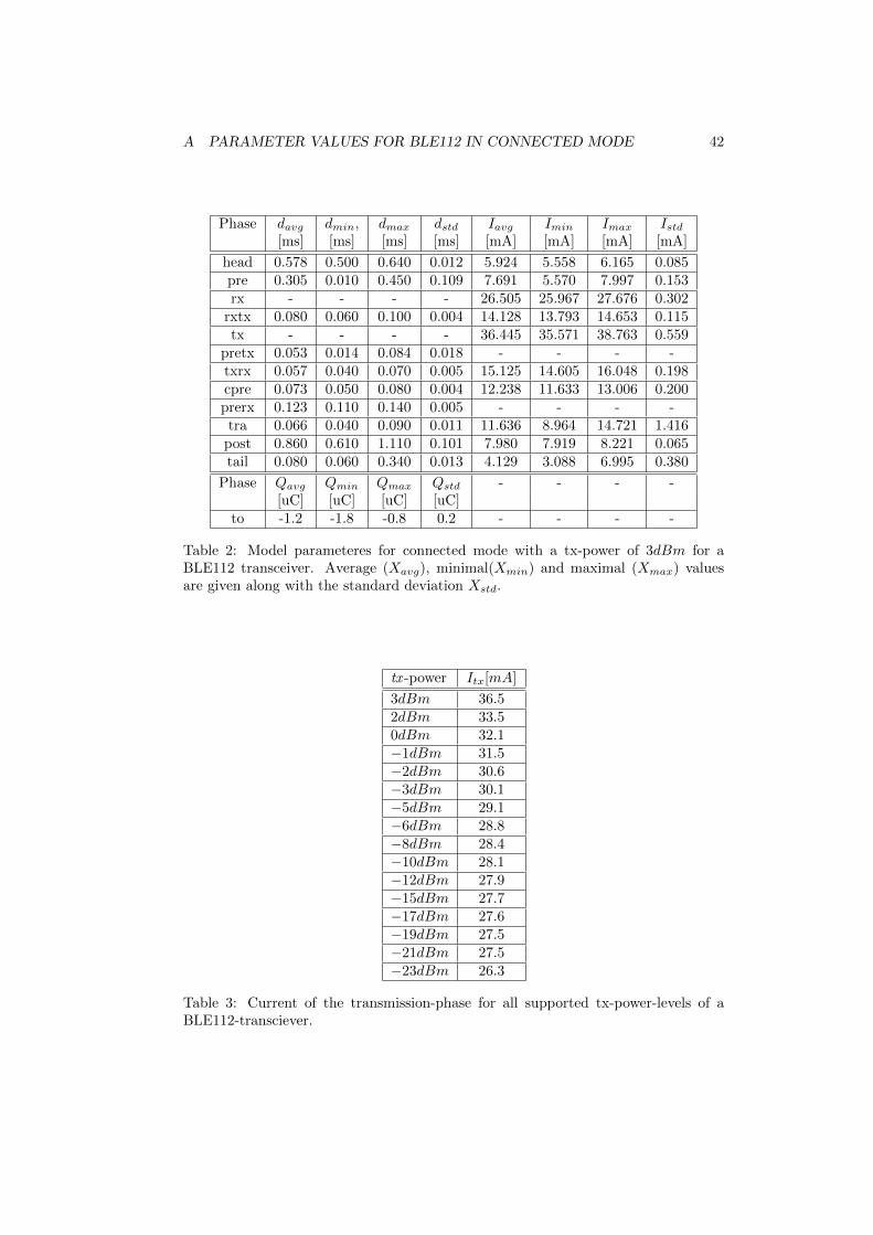
A PARAMETER VALUES FOR BLE112 IN CONNECTED MODE 42
Phase davg dmin, dmax dstd Iavg Imin Imax Istd[ms] [ms] [ms] [ms] [mA] [mA] [mA] [mA]
head 0.578 0.500 0.640 0.012 5.924 5.558 6.165 0.085pre 0.305 0.010 0.450 0.109 7.691 5.570 7.997 0.153rx - - - - 26.505 25.967 27.676 0.302
rxtx 0.080 0.060 0.100 0.004 14.128 13.793 14.653 0.115tx - - - - 36.445 35.571 38.763 0.559
pretx 0.053 0.014 0.084 0.018 - - - -txrx 0.057 0.040 0.070 0.005 15.125 14.605 16.048 0.198cpre 0.073 0.050 0.080 0.004 12.238 11.633 13.006 0.200prerx 0.123 0.110 0.140 0.005 - - - -tra 0.066 0.040 0.090 0.011 11.636 8.964 14.721 1.416
post 0.860 0.610 1.110 0.101 7.980 7.919 8.221 0.065tail 0.080 0.060 0.340 0.013 4.129 3.088 6.995 0.380
Phase Qavg Qmin Qmax Qstd - - - -[uC] [uC] [uC] [uC]
to -1.2 -1.8 -0.8 0.2 - - - -
Table 2: Model parameteres for connected mode with a tx-power of 3dBm for aBLE112 transceiver. Average (Xavg), minimal(Xmin) and maximal (Xmax) valuesare given along with the standard deviation Xstd.
tx -power Itx[mA]
3dBm 36.52dBm 33.50dBm 32.1−1dBm 31.5−2dBm 30.6−3dBm 30.1−5dBm 29.1−6dBm 28.8−8dBm 28.4−10dBm 28.1−12dBm 27.9−15dBm 27.7−17dBm 27.6−19dBm 27.5−21dBm 27.5−23dBm 26.3
Table 3: Current of the transmission-phase for all supported tx-power-levels of aBLE112-transciever.

B PARAMETER VALUES FOR BLE112 IN SCANNING MODE 43
B Parameter values for BLE112 in scanning mode
The table below presents values for all model parameters for the scanning mode. They wereobtained by analyzing 1257 scan events for a tx-power of 3dBm.
Part davg dmin, dmax dstd Iavg Imin Imax Istd[ms] [ms] [ms] [µs] [mA] [mA] [mA] [mA]
pre,s 0.700 0.680 0.730 10 7.087 6.924 7.253 0.065rx,s - - - - 26.399 26.042 26.480 0.043
rxtx,s 0.115 0.110 0.120 0.498 15.011 14.617 15.519 0.288tx,s - - - - 35.999 35.650 36.488 0.247
pretx,s 0.014 4e-3 0.024 1.184 - - - -txrx,s 0.089 0.080 0.090 2.332 16.670 15.875 17.224 0.244rxsr - - - - 26.426 26.279 26.563 0.058
prerx,s 0.074 0.068 0.088 2.45 - - - -rxrx,s 0.377 0.370 0.380 4.488 9.633 9.426 9.768 0.11post,s 0.816 0.710 1.820 246 8.012 7.820 8.138 0.060chch,s 1.325 1.320 1.330 4.983 8.550 8.470 8.624 0.042
Part Qavg Qmin Qmax Qstd - - - -[uC] [uC] [uC] [uC]
ctx,s -0.2264 -0.3244 -0.1456 0.0143 - - - -crx,s -0.1350 -0.1900 -0.0851 0.0123 - - - -
Table 4: Model parameter values for scan events. Average (Xavg), minimal(Xmin)and maximal (Xmax) values are given along with the standard deviation Xstd.
C Table of symbols
The symbol X stands either for the charge Q, the current I or the duration d of a phase ofa connection event.
BLE Protocol
Symbol Unit Description
Ta [s] Advertising interval
Ts [s] Scan interval
ds [s] Scan window
dIFS [s] Interframe-space
ρ(t) [s] Random advertising delay
dtw [s] Transmit window
dtwo [s] Transmit window offset
tanchor [s] Anchor point: Reference point for connection interval
Tc [s] Connection interval
Tc,o [s] Connection interval before a connection parameter up-date
Tc,n [s] Connection interval after a connection parameter update
dc [s] Duration of a connection event
Nsl - Slave latency
dadv [s] Expected discovery latency in the advertising/scanningmode

C TABLE OF SYMBOLS 44
Single event model for the connected mode
Symbol Unit Description
Xhead [C/A/s] Device wakeup phase
Xpre [C/A/s] Preprocessing phase
Xcpre [C/A/s] Communication preamble phase
Xww [C/A/s] Window widening phase
Xprerx [C/A/s] Constant part of reception phase
Xrx [C/A/s] Reception phase
Nrx - Number of bytes received
XIFS [C/A/s] Interframe space
Xrxtx [C/A/s] Reception-to-transmission transition phase
Xtxrx [C/A/s] Transmission-to-reception transition phase
Xpretx [C/A/s] Constant part of transmission phase
Xtx [C/A/s] Transmission phase
Ntx - Number of bytes sent
Xtra [C/A/s] Transient phase
Xpost [C/A/s] Postprocessing phase
Xtail [C/A/s] Tail phase (i.e., phase that initiates of the sleep mode)
dseq [s] Duration of a communications sequence (i.e., exchangeof one pair of packets)
devent [s] Duration of a whole connection event (from head to tail)
Xt [C/A/s] Communication sequence (reception, transmission,interframe-spaces and correction term for capaci-tances/resistances)
Qto [C] Correction term for capacitances/resistances in powersupply line
SCAMa/Sl [ppm] Sleep clock accuracy of master/slave
Isl [A] Sleep current of the BLE device
Single event model for scan events
Symbol Unit Description
Xpre [C/A/s] Wakeup and preprocessing phase
XS,1 [C/A/s] Phase of scanning until the first reception takes place
Xrx,s [C/A/s] Reception phase (advertising packet is received)
Xrxtx,s [C/A/s] Reception-to-transmission transition phase
Xtx,s [C/A/s] Transmission of scan-request (or connection request)phase
Xtxrx,s [C/A/s] Transmission-to-reception transition phase
Xrxs [C/A/s] Phase of the reception of a scan response
Xrxrx,s [C/A/s] Reception-to-scanning transition phase
XS,2 [C/A/s] Phase of scanning until the end of the scan event
Xpost,s [C/A/s] Postprocessing phase
Iscan [A] Current consumption of the device while scanning
QsEv [C] Charge consumed by a scan event (general case)
QsEv,Idle [C] Charge consumed by a scan event (idle scanning)
Qcrx,s [C] Correction term for non-rectangular shapes of thereception-phase(s)
Qctx,s [C] Correction term for non-rectangular shapes of thetransmission-phase(s)
Connection procedure model
Symbol Unit Description

C TABLE OF SYMBOLS 45
Qev,cR,Ma/Sl [C] Charge consumed by the master/slave for an event a con-nection request event is sent within
Qev,cU,Ma/Sl [C] Charge consumed by the master/slave for an event a con-nection update packet is sent within
dsl,cR/cU [s] Sleep duration after a connection request/update event
QcE,Ma/Sl [C] Charge consumed for a connection establishment by themaster/slave
QcU,Ma/Sl [C] Charge consumed for a connection parameter update bymaster/slave
dp [s] Time from beginning of the transmit window until themaster sends the first packet with new Tc
dww,cE/cU [s] Window widening for connection establish-ment/parameter update
Discovery Latency Model
Symbol Unit Description
dadvPkg [s] Duration of an advertising packet
φ [s] Offset between the beginning of the first scan event andthe first advertising event
Ta,0 [s] Constant part of the advertising interval
ρ [s] Random delay for advertising events
ti,suc [s] Set of points in time an advertising packet which is sentwithin is received successfully
dearly [s] Time an advertising event can be sent before the be-ginning of the corresponding scan event to be receivedsuccessfully
dlate [s] Time an advertising event must be sent before the end ofthe corresponding scan event to be received successfully
d′s [s] Effective scan window (d′s = ds − da)
da [s] Duration of an advertising packet
dch [s] Time the advertiser needs for changing the channel itsends its packets on
tsE [s] Time a scan event starts at
tadvEvt [s] Time an advertising event is sent at
phit(n) - Probability of an advertising event n for hitting a scanevent
f(ρ) - Probability density function for the random advertisingdelay
µ - Expected value
σ - Standard deviation
f(tadvEvt) - Probability density function for the beginning of an ad-vertising event
pk - Probability for an advertising event being received in thescan event k
Φ(t) - Standard normal cumulative distribution
tai [s] Point in time an advertising event would take place with-out taking the random delay ρ into account
kmin(n),kmax(n)
- Lowest and highest index of a scan event the advertisingevent n could overlap with
pcM (n) - Cumulative miss probability (probability that n adver-tising events in a row miss the scan event)
dexp [s] Expected advertising duration for a given pair of valuesΦ and k

C TABLE OF SYMBOLS 46
ε - Parameter of Algorithm 1 that determines the precisenessand computational complexity
ch - Channel number (37/38/39)
dexp,max [s] Maximum expected advertising duration for a given pairof values φ and k before the calculation is aborted
∆ [s] Interval between two offsets φ that are examined
dadv [s] Expected discovery latency
P37/P38/P39 - Reception probability on channel 37/38/39 in the con-stant scanning mode
Ploss - Probability that the first advertising packet is lost in theconstant scanning mode
dadv,max [s] Maximum possible discovery latency in the constantscanning mode
h1, h2, h3, A,B, C
var. Helper functions for constant scanning model
Estimating the number of events
Symbol Unit Description
Nc,ma/sl - Number of connection events of the master/slave withina given amount of time
Qcon [C] Overall charge consumed by the master/slave in the con-nected mode
Tg [s] Given amount of time which is considered
Nsl - Average slave latency
Xevent [C/A/s] Charge/current/duration of an arbitrary event
Xfull [C/A/s] Full advertising event
Xlast [C/A/s] Last advertising event
Qadv [C] Expected charge consumed by an advertiser (whole dis-covery process)
QadvEvent [C] Charge consumed by an advertising event
X37(38/39) [C/A/s] Advertising event on channel 37/38/39
Na - Expected number of advertising events
Qs [C] Expected Energy of scanner (whole discovery process)
Qactive [C] Expected charge of scanner for all times it is not sleeping
Qsleep [C] Expected charge of scanner for all times it is sleeping
QsEv,idle [C] Charge consumed by an idle scan event (i.e., scan eventwithout reception)
Na, Ns [C] Expected number of advertising/scan events duringneighbor discovery
Model validation and sensitivity analysis
Symbol Unit Description
εm - Relative error between measured and modeled values
S var. Sensitivity
Qph [C] Charge consumed by a phase/state the device is in (e.g.,preprocessing, reception,..)
dmin/dmax [s] Minimum/maximum phase duration
Imin/Imax [A] Minimum/maximum current of a phase
δQtotal [C] Variation of the total charge consumed in a given phase
η [Bytes/C] Efficiency