PhD thesis: Indefinite Focusing - Electrical and Computer Engineering
102
UNIVERSITY OF CALIFORNIA, SAN DIEGO Indefinite Focusing A dissertation submitted in partial satisfaction of the requirements for the degree Doctor of Philosophy in Physics by David Schurig Committee in charge: Professor Sheldon Schultz, Chairperson Professor Norman M. Kroll Professor Dimitri N. Basov Professor Paul K. Yu Professor Alan M. Schneider Professor Marshall N. Rosenbluth 2002
Transcript of PhD thesis: Indefinite Focusing - Electrical and Computer Engineering

UNIVERSITY OF CALIFORNIA, SAN DIEGO
Indefinite Focusing
A dissertation submitted in partial satisfaction of the
requirements for the degree Doctor of Philosophy
in Physics
by
David Schurig
Committee in charge:
Professor Sheldon Schultz, ChairpersonProfessor Norman M. KrollProfessor Dimitri N. BasovProfessor Paul K. YuProfessor Alan M. SchneiderProfessor Marshall N. Rosenbluth
2002


The dissertation of David Schurig is approved, and it is
acceptable in quality and form for publication on micro-
film:
Chair
University of California, San Diego
2002
iii

TABLE OF CONTENTS
Signature Page . . . . . . . . . . . . . . . . . . . . . . . . . . . . . . . . iii
Table of Contents . . . . . . . . . . . . . . . . . . . . . . . . . . . . . . iv
List of Figures . . . . . . . . . . . . . . . . . . . . . . . . . . . . . . . . vi
Acknowledgements . . . . . . . . . . . . . . . . . . . . . . . . . . . . . x
Vita and Publications . . . . . . . . . . . . . . . . . . . . . . . . . . . . xi
Abstract . . . . . . . . . . . . . . . . . . . . . . . . . . . . . . . . . . . xii
I Negative Refraction of Modulated Electromagnetic Waves . . . . . . . . 1A. Abstract . . . . . . . . . . . . . . . . . . . . . . . . . . . . . . . . . 1B. Letter . . . . . . . . . . . . . . . . . . . . . . . . . . . . . . . . . . . 1C. Acknowledgement . . . . . . . . . . . . . . . . . . . . . . . . . . . . 9
II Focusing Properties of a Slab of Negative Index Media . . . . . . . . . . 10A. Abstract . . . . . . . . . . . . . . . . . . . . . . . . . . . . . . . . . 10B. Introduction . . . . . . . . . . . . . . . . . . . . . . . . . . . . . . . 10C. Description of Perfect Image Evolution . . . . . . . . . . . . . . . . 12D. The Boundary Value Problem . . . . . . . . . . . . . . . . . . . . . 13E. Image Resolution: Approximate Analytical Results . . . . . . . . . . 22F. Source Object . . . . . . . . . . . . . . . . . . . . . . . . . . . . . . 24G. k-Space Mesh . . . . . . . . . . . . . . . . . . . . . . . . . . . . . . 25H. Image Resolution: Numerical Results . . . . . . . . . . . . . . . . . 261. transfer function . . . . . . . . . . . . . . . . . . . . . . . . . . . 262. Spatial Images . . . . . . . . . . . . . . . . . . . . . . . . . . . . 373. Z Field Dependence . . . . . . . . . . . . . . . . . . . . . . . . . 38
I. Aperture . . . . . . . . . . . . . . . . . . . . . . . . . . . . . . . . . 39J. Conclusion . . . . . . . . . . . . . . . . . . . . . . . . . . . . . . . . 39K. Acknowledgement . . . . . . . . . . . . . . . . . . . . . . . . . . . . 41L. Material Parameters Simulated . . . . . . . . . . . . . . . . . . . . . 41
III Electromagnetic Wave Propagation in Media with Indefinite Permittiv-ity and Permeability Tensors . . . . . . . . . . . . . . . . . . . . . . . . 44A. Abstract . . . . . . . . . . . . . . . . . . . . . . . . . . . . . . . . . 44B. Introduction . . . . . . . . . . . . . . . . . . . . . . . . . . . . . . . 44C. Media . . . . . . . . . . . . . . . . . . . . . . . . . . . . . . . . . . . 46D. Refraction and Reflection . . . . . . . . . . . . . . . . . . . . . . . . 49E. Layered Media: Focusing . . . . . . . . . . . . . . . . . . . . . . . . 53
iv

F. Conclusion . . . . . . . . . . . . . . . . . . . . . . . . . . . . . . . . 55G. Acknowledgement . . . . . . . . . . . . . . . . . . . . . . . . . . . . 57
IV Sub-Diffraction Focusing Using Bilayers of Indefinite Media . . . . . . . 58A. Abstract . . . . . . . . . . . . . . . . . . . . . . . . . . . . . . . . . 58B. Introduction . . . . . . . . . . . . . . . . . . . . . . . . . . . . . . . 58C. Dispersion . . . . . . . . . . . . . . . . . . . . . . . . . . . . . . . . 59
D. General Bilayer Solution . . . . . . . . . . . . . . . . . . . . . . . . 62E. Simplest Case . . . . . . . . . . . . . . . . . . . . . . . . . . . . . . 64
F. Asymmetric Bilayers and Field Plots . . . . . . . . . . . . . . . . . . 67
G. Lossy Media: Approximate Analytical Transfer Function . . . . . . . 68H. Conclusion . . . . . . . . . . . . . . . . . . . . . . . . . . . . . . . . 71I. Acknowledgement . . . . . . . . . . . . . . . . . . . . . . . . . . . . 72
V Electromagnetic Spatial Filtering Using Media with Negative Properties 73A. Abstract . . . . . . . . . . . . . . . . . . . . . . . . . . . . . . . . . 73B. Introduction . . . . . . . . . . . . . . . . . . . . . . . . . . . . . . . 73C. Dispersion . . . . . . . . . . . . . . . . . . . . . . . . . . . . . . . . 75D. Transfer Matrix . . . . . . . . . . . . . . . . . . . . . . . . . . . . . 77
E. Spatial Filters . . . . . . . . . . . . . . . . . . . . . . . . . . . . . . 79F. Conclusion . . . . . . . . . . . . . . . . . . . . . . . . . . . . . . . . 86G. Acknowledgement . . . . . . . . . . . . . . . . . . . . . . . . . . . . 86
Bibliography . . . . . . . . . . . . . . . . . . . . . . . . . . . . . . . . . 87
v

LIST OF FIGURES
I.1 Normal incidence (A). The group velocity and interference wavevector are parallel. Incidence at 45 degree angle (B). On the incidentside (left) the component wave vectors, interference wave vector andgroup velocity all point in the same direction. In the NIM (right) theinterference wave vector has refracted positively and the componentwave vectors and group velocity have refracted negatively with thecomponent wave vectors approximately anti-parallel to the groupvelocity. The dashed lines indicate conservation of the transversecomponent of the various wave vectors. . . . . . . . . . . . . . . . . 3
I.2 Refraction of a Gaussian beam into a NIM. The angle of incidenceis 30 degrees. n (ω−) = −1.66+0.003i and n (ω+) = −1.00+0.002i.∆ω/ω = 0.07. . . . . . . . . . . . . . . . . . . . . . . . . . . . . . . 8
II.1 Spatial evolution of field distribution through a perfect lens slab.Both slab interfaces are mirror planes for the field distribution.(Field profiles are not uniformly scaled.) . . . . . . . . . . . . . . . 14
II.2 Labeling conventions for boundary value problem. . . . . . . . . . . 16II.3 Location of focii. The two focii occur at the locations marked z1.
The source is at z0. . . . . . . . . . . . . . . . . . . . . . . . . . . 21II.4 Values of µ and ² simulated are shown in the complex plane. For
each value of µ and ², the transfer function and a real space imagehave been calculated. Positive real deviations lead to symmetricmodes and negative real deviation lead to antisymmetric modes. µdeviations are shown in figure II.5 and II.7 ε deviations in figuresII.6 and II.8. . . . . . . . . . . . . . . . . . . . . . . . . . . . . . . 27
II.5 The transfer function of the slab. In this and subsequent figuresthe parameter that deviates from -1 is indcated in the upper rightcorner. The direction of the deviation in the complex plane isindicated by an arrow. Lighter shading of the line indicates largerdeviation. The dashed line is the largest deviation that can stillresolve λ/10 features. . . . . . . . . . . . . . . . . . . . . . . . . . . 28
II.6 The solid circles mark the points for which z field dependence isshown. Circles in the top pane correspond to figure II.11 and circlesin third pane correspond to figure II.12. . . . . . . . . . . . . . . . . 29
II.7 Intensity of object and image focused by slab. The object is twosquare peaks of unit intensity, width λ/100 and separation λ/10. . . 30
II.8 Intensity of object and image focused by slab. The object is twosquare peaks of unit intensity, width λ/100 and separation λ/10. . . 31
vi

II.9 Resonance merge. The dashed line in the upper two panes is forthe value of µ that merges the two resonances. The bottom paneshows the center, (x = 0), intensity versus µ. This intensity peaksat the merge, µ = −0.45. . . . . . . . . . . . . . . . . . . . . . . . . 32
II.10 Resonance merge. The dashed line in the upper two panes is forthe value of ² that merges the two resonances. The bottom paneshows the center, (x = 0), intensity versus ². This intensity peaksat the merge, ² = 3.45. . . . . . . . . . . . . . . . . . . . . . . . . . 33
II.11 Z dependence of the electric field excited by a unit plane wave ofthe specified transverse wave vector, kx. The slab is delineated bythe vertical grey lines. The solid line is for µ = −1, ² = 1, and thedashed line is for µ = ² = −1. The phase is indicated by shadingas shown in the legend. . . . . . . . . . . . . . . . . . . . . . . . . . 34
II.12 Z dependence of the electric field excited by a unit plane wave of thespecified transverse wave vector, kx. The slab is delineated by thevertical grey lines. The solid line is for µ = −1, ² = −3, and thedashed line is for µ = ² = −1. The phase is indicated by shading asshown in the legend. . . . . . . . . . . . . . . . . . . . . . . . . . . 35
II.13 Geomtric arrangement of aperature slab. . . . . . . . . . . . . . . . 39II.14 Image plane field for aperatured slab. . . . . . . . . . . . . . . . . . 40
III.1 Iso-frequency curves for different classes of media. The cutoff trans-verse wave vector, kc, is indicated for the cutoff and anti-cutoffmedia. Solid lines indicate real valued kz. Dashed lines indicateimaginary values. . . . . . . . . . . . . . . . . . . . . . . . . . . . 48
III.2 Each medium class has two sub-types, positive and negative. Thesub-type indicates the direction of refraction, or equivalently, thesign of the z-component of the group velocity relative to the wavevector. Negation of both µ and ε switches the sub-type. (Forease of illustration, the tensors in this table and those used for allspecific calculations and plots in this article have elements of unitmagnitude.) . . . . . . . . . . . . . . . . . . . . . . . . . . . . . . 50
III.3 Refraction from free space (blue) into negative, (green) and positive,(red) always propagating media. Only the real parts of the disper-sion curves are shown. The free space curve is black and the alwayspropagating medium is gray. The white, construction lines indicatethe conservation of transverse wave vector, etc. The lengths of thegroup velocity vectors are not shown to scale. . . . . . . . . . . . . 51
III.4 Magnitude of the transfer function vs. transverse wave vector. Thedevice is a bi-layer of positive and negative always propagating ma-terial with layers of equal thickness, L1/λ = 0.1, 0.2, 0.5, 1, 2. Thethinnest layer is the darkest curve. A realistic loss of 0.01i has beenadded to each diagonal component of ε and µ. . . . . . . . . . . . . 54
vii

III.5 Split ring resonators are shown in black. Wires are shown in gray.Upper device: layer one has split ring resonators oriented in the xdirection and wires in the y direction, and layer two has split ringresonators in the z direction. Lower device: layer one has split ringresonators oriented in the y direction and wires in the x direction,and layer two has wires in the z direction. . . . . . . . . . . . . . . 56
IV.1 Hyperbolic dispersion found in always propagating media (black).The asymtotic behavior is also shown (white.) Two wave vectorsare shown that have the same transverse component, kx. Bothpossible group velocity directions are shown for each wave vector.The normal (z) component of k and vg can be either of the samesign or opposite sign. . . . . . . . . . . . . . . . . . . . . . . . . . . 61
IV.2 From top to botton: 1. the indices used to refer to material proper-ties, 2. the conventions for the coefficients of each component of thegeneral solution, 3.the sign structure of the material property ten-sors, 4. typical z-dependence of the electric field for an evanescentincident plane wave, 5. z-coordinate of the interfaces. . . . . . . . . 62
IV.3 The magnitude of coefficients of the internal field components. Forvalues of kx > k0 (incident plane wave is evanescent) the forwardand backward components have equal magnitude. The magnitudeapproaches 1/
√2 when kx À k0. . . . . . . . . . . . . . . . . . . . . 66
IV.4 Internal electric field intensity plot for a localized two slit source.The four vector pairs in each layer indicate the only four orientationsof internal plane waves. Plane waves from positve kx componentsof the source are indicated in white and negative in gray. Thewave vectors are labeled with the solution component to which theycorresond. kA and kC have positve z-components and kB and kDhave negative z-components. The unmarked vector in each pairindicates the direction of the group velocity for that plane wavedirection. m1 = 1 and m2 = 1/2. . . . . . . . . . . . . . . . . . . . 69
IV.5 The transfer function from the front surface to the back surface ofthe bilayer. z1 = z2 − z1 = λ, m = 1/3 and ε00 = µ00 = .001, .002,.005, .01, .02, .05, .1, from light to dark. For comparison, a singlelayer, isotropic near field lens is shown dashed. The single layer hasthickness, λ, and ε = µ = −1 + 0.001i. . . . . . . . . . . . . . . . . 70
V.1 Dispersion curves for cutoff and anti-cutoff media for several dif-ferent values of the cutoff, kc. Solid lines indicate real valued kz,and dashed lines indicate imaginary values. A wave vector, k, isshown, and both possible group velocity directions associated withthat wave vector. . . . . . . . . . . . . . . . . . . . . . . . . . . . . 76
viii

V.2 Reflection and transmission coefficients versus incident angle for low,high and band pass filters. For the high and low pass filters, thevalues for θc ≡ sin−1 (kc/k0) are π/12, π/6, π/4, π/3 and 5π/12going from dark to light lines. The band pass filter has cutoffs, π/6and π/3, with transmission shown with a dark line and reflectionshown with a light one. γ = 0.01 and k0d = 4π for all filters exceptθc ≡ π/12 where k0d = 6π. . . . . . . . . . . . . . . . . . . . . . . . 80
V.3 Reflection and transmission coefficients versus transverse wave vec-tor, kx/k0, for low, high and band pass filters. For the high andlow pass filters, the values for kc/k0 are 1, 2, 5, 10 and 20 goingfrom dark to light lines. The band pass filter has cutoffs, 5 and 10,with transmission shown with a dark line and reflection shown witha light one. γ = 0.01 and kcd = 4π for all filters; the filters withhigher cutoffs are thinner. . . . . . . . . . . . . . . . . . . . . . . . 81
V.4 Reflection and transmission of Gaussian beams incident on a bandpass filter. The band pass filter has θc = 24 and 58, kcd = 4π,and γ = 0.01. The beams have width 10λ0 and incident angles 9
,34, and 69. The scale on the transmission side is compressed tocompensate for the attenuation of the beam. . . . . . . . . . . . . . 82
V.5 Low, high and band pass filtering of a square wave object. Thesquare wave has a fundamental period of λ0. The low pass filterhas cutoff, kc/k0 = 5. The band pass filter has cutoffs, kc/k0 = 5and 20, and the high pass filter has cutoff, kc/k0 = 20. γ = 0.01and kcd = 4π for all three filters. . . . . . . . . . . . . . . . . . . . . 83
ix

ACKNOWLEDGEMENTS
Each chapter of this thesis has or will be submitted for publication as listed below:
D. R. Smith, D. Schurig, J. B. Pendry; Negative Refraction of Modulated Elec-
tromagnetic Waves, submitted for publication, Applied Physics Letters.
D. Schurig, D. R. Smith, S. Schultz, S. A. Ramakrishna, J. B. Pendry; Focusing
Properties of a Slab of Negative Index Media, not yet submitted.
D. R. Smith and D. Schurig; Electromagnetic Wave Propagation in Media with
Indefinite Permittivity and Permeability Tensors, submitted to Physical Re-
view Letters.
D. Schurig and D. R. Smith ; Sub-Diffraction Imaging with Compensated Bilayers
of Indefinite Media, not yet submitted.
D. Schurig and D. R. Smith; Electromagnetic Spatial Filtering Using Media with
Negative Properties, not yet submitted.
I would like to thank the following people: Daniel Schurig, Diane Schurig,
Darren Schurig, Sheldon Schultz, David Smith, John Pendry, Alan Schneider, Nor-
man Kroll, the rest of my thesis defense committee, Andy Pommer, George Kass-
abian, Matt Pufall, Sang Park, Willie Padilla, Joan Marler, Jason Goldberg, Erik
Stauber, Jason Feinberg, Syrus Nemat-Nasser, Stephen Wolfram, John Jackson,
James Maxwell, Tony Starr, Tatiana Starr, Douglas Paulson, everyone at Tristan
Technologies Inc., the UCSD cycling team, the UCSD triathlon team, CalSpace,
Kevin the Hari Krishna, and the UCSD physics graduate class of 1991.
x

VITA
19 March 1966 Born, Burbank, California
1989 B.S. Engineering Physics, University of California, Berke-ley
2002 Doctor of Philosophy, Physics, University of Califor-nia, San Diego
PUBLICATIONS
“Large magnetoresistance in La-Ca-Mn-O films.” IEEE Transactions on Magnetics,vol.31, (no.6, pt.2), Nov. 1995. p.3912-14
“Thickness dependence of magnetoresistance in La-Ca-Mn-O epitaxial films.” Ap-plied Physics Letters, vol.67, (no.4), 24 July 1995. p.557-9
xi

ABSTRACT OF THE DISSERTATION
Indefinite Focusing
by
David Schurig
Doctor of Philosophy in Physics
University of California, San Diego, 2002
Professor Sheldon Schultz, Chair
It is shown that a modulated Gaussian beam undergoes negative refrac-
tion at the interface between a positive and negative refractive index material.
While the refraction of the beam is clearly negative, the modulation interference
fronts are not normal to the group velocity, and thus exhibit a sideways motion
relative to the beam-an effect due to the inherent frequency dispersion associated
with the negative index medium
A slab of negative index media has been shown to focus both the far-field
and the near-field of an electromagnetic source and form an image with resolution
better than what is possible with diffraction limited, conventional optics. How-
ever, deviations from the ideal material properties, such as dissipation, limit the
image resolution. A wide range of the material property parameter space is stud-
ied, demonstrating the limits of resolution with numerical results and approximate
analytical formulas. The effects of a finite aperture on the imaging are also exam-
ined.
Wave propagation in materials for which not all of the principle elements
of the permeability and permittivity tensors have the same sign is studied. These
tensors are neither positive nor negative definite. It is found that a wide variety
of effects can be realized in such media, including negative refraction, near-field
focusing and high impedance surface reflection.
xii

A new type of near field focusing device is analyzed that consists of a
bilayer of media with indefinite electromagnetic material property tensors. The
dispersion of the media supports propagating waves for any transverse wave vector,
which results in a weaker dependence of spatial bandwidth on media lossiness.
We show how bilayers of media with negative electromagnetic property
tensor elements can be used to construct low, high and band pass spatial filters.
These filters possess sharp adjustable roll offs and can operate in the near and far
field regimes to select specific spatial variation components or beam angles.
xiii

Chapter I
Negative Refraction of Modulated
Electromagnetic Waves
I.A Abstract
We show that a modulated Gaussian beam undergoes negative refraction
at the interface between a positive and negative refractive index material. While
the refraction of the beam is clearly negative, the modulation interference fronts
are not normal to the group velocity, and thus exhibit a sideways motion relative
to the beam-an effect due to the inherent frequency dispersion associated with
the negative index medium. In particular, the interference fronts appear to bend
in a manner suggesting positive refraction, such that for a plane wave, the true
direction of the energy flow associated with the refracted beam is not obvious.
I.B Letter
Since the experimental demonstrations of a structured metamaterial with
simultaneously negative permittivity and negative permeability [1, 2]-often referred
to as a left-handed material, the phenomenon of negative refraction, predicted to
occur in left-handed materials [3, 4], has become of increasing interest. The con-
sequence of a modulated plane wave incident on an infinite half-space of negative
1

2
refractive index material has been considered by Valanju et al. [5], who have
noted that the interference fronts due to the modulation appear to undergo posi-
tive refraction, despite the underlying negative refraction of the component waves.
Valanju et al. further associate the direction of the advancing interference pattern
with that of the group velocity, and draw a broad set of conclusions regarding the
validity of negative refraction.
In this letter, we examine the effect of a finite-width beam refracting at
the interface between two semi-infinite media, one with positive refractive index
and the other with negative refractive index. We find that the transmitted beam
does indeed refract in the negative direction, although the interference fronts do
not necessarily point in the same direction. We first describe the refraction of a
modulated plane wave incident on a half-space with negative index, which demon-
strates in a straightforward manner, that the interference fronts of the transmitted
wave display interesting behavior.
We assume the geometry shown in Fig. I.1, in which a modulated electro-
magnetic wave is incident from vacuum onto a material with frequency dependent,
negative index of refraction, n(ω). We choose the z-axis normal to the interface,
the x-axis in the plane of the figure, and the y-axis out of the plane of the figure.
While our arguments will apply to a wave with arbitrary polarization, we assume
here that the electric field is polarized along the y-axis (out of plane). For con-
venience, we use identical causal plasmonic forms for the permittivity (ε) and the
permeability (µ), so that the refractive index is given by
n (ω) =√εµ = 1− ω2p
ω (ω + iΓ). (I.1)
Note that the refractive index is negative below the plasma frequency ωp, and has
the value of approximately −1 when ω = ωp/√2and losses are small, Γ/ω ¿ 1.
A modulated plane wave has the form
E (r, t) = eik·re−iΩt cos (∆k · r−∆ωt) , (I.2)

3
Figure I.1: Normal incidence (A). The group velocity and interference wave vec-
tor are parallel. Incidence at 45 degree angle (B). On the incident side (left) the
component wave vectors, interference wave vector and group velocity all point in
the same direction. In the NIM (right) the interference wave vector has refracted
positively and the component wave vectors and group velocity have refracted neg-
atively with the component wave vectors approximately anti-parallel to the group
velocity. The dashed lines indicate conservation of the transverse component of
the various wave vectors.

4
where Ω is the carrier frequency of the wave, ∆ω is the modulation frequency and
the wave vector, k, is given in terms of the incident angle,
k = sin (θ) kbx+ cos (θ) kbz (I.3)
where k = ω/c. Eq. I.3 can be equivalently viewed as the superposition of two
plane waves with different frequencies, or
E (r, t) =1
2eik+·re−iω+t +
1
2eik−·re−iω−t
where the frequencies of the component waves are ω± = ω±∆ω with corresponding
propagation vectors k± = k±∆k. ∆k is parallel to k and is given by
∆k =∆ω
ωk (I.4)
Because the negative index medium is assumed to be frequency dispersive, the
transmitted waves will refract at slightly different angles, thus introducing a dif-
ference in the phase versus interference propagation directions. The transmitted
wave can be expressed in the form
E (r, t) = eiq·re−iΩt cos (∆q · r−∆ωt) , (I.5)
which again is composed of two propagating plane waves having propagation vec-
tors q+ and q−, the values of which can be found using the conservation of the
parallel wave vector across the interface
qx = kx (I.6)
and the constancy of frequency,
q · q = n2k2 (I.7)
resulting in
q = kxbx±pn2k2 − k2xbz (I.8)

5
The correct sign of this expression for individual plane waves is well established
elsewhere [6, 7]. Using ∆qx = ∆kx and Eq. I.7, the wave vector of the interference
pattern is obtained.
∆q =
·kxbx+ 1
qz
¡k2nng − k2x
¢bz¸ ∆ω
Ω(I.9)
The group index, given by
ng ≡ ∂ (nω)
∂ω≥ 1
is constrained by causality to be greater than unity regardless of the sign of the re-
fractive index of the medium. Thus, we see that for a negative refractive index the
z-component of the interference wave vector has opposite sign to the z-component
of the individual wave vectors, so though the individual wave vectors refract neg-
atively, the interference pattern refracts positively. Furthermore, the apparent
velocity of the interference fronts is directed away from the interface, as would
be expected if the direction of the interference pattern were coincident with the
direction of the group velocity. Note that Eq. I.9 also implies that the spacing
between interference fronts (or beats) in the negative index medium is set by the
dispersion characteristics of the medium rather than just the frequencies of the
two component waves. This effect is illustrated in Fig. I.1A for a wave normally
incident from vacuum on a medium with a frequency dispersive negative refractive
index. In this example, the carrier frequency is assumed to be at the frequency
where n = −1. For our choice of frequency dispersion (Eq. I.1), ∂(nω)∂ω
= 3, and
Eq. I.9 shows that the spacing between interference fronts is one-third that in free
space, as seen in the figure.
When a monochromatic wave is incident on the interface between positive
and negative media at an angle, previous calculations and theory [1, 3] have shown
that the phase velocity is negative, and the transmitted ray in the medium is
directed toward the interface and negatively refracted. Eq. I.9, however, indicates
that the interference fronts associated with a modulated plane wave should undergo
positive refraction. A calculation of the refraction of a modulated plane wave shows

6
that this is indeed the case (Fig. I.1B): the incident interference pattern refracts
to the opposite side of the normal, consistent with Valanju et al. [5].
The question thus naturally arises: what is the relationship between the
interference fronts associated with a modulated wave and its group velocity? The
group velocity is defined as [8]
vg ≡ ∇qω (q) , (I.10)
which, for isotropic, low loss materials becomes
vg =q
q
dω (q)
dω=q
qsign (n)
c
ng. (I.11)
The scalar part of this expression is a material property and the unit vector pre-
factor is a determined by the direction of the incoming wave. Note that when the
index is negative, Eq. I.11 predicts that the direction of the group velocity is anti-
parallel to the phase velocity, and thus refracts negatively-unlike the interference
wave vector. This would seem to be a paradox, as the interference velocity of
a modulated beam is frequently equated with the group velocity [8]. To resolve
this dilemma, we examine the manner in which a point of constant phase on the
interference patterns moves. Setting the argument of the Cosine in Eq. I.5 equal
to a constant, we find that the velocity of such a point, vint, must satisfy
∆q
∆ω· vint = 1 (I.12)
The smallest possible such velocity is the one parallel to ∆q (the interference
direction), which has been interpreted as the group velocity by Valanju et al. [5];
however, vint can have an arbitrary component perpendicular to ∆q. For non-
normal incidence, the group velocity has such a component. Using Eqs. I.9 and
I.11, we can verify that the group velocity does indeed satisfy Eq. I.12. We thus
conclude that a component of the group velocity follows the interference pattern,
but that there is also a component parallel to the interference wave fronts.
Since we have concluded that the interference velocity need not be in the
same direction as the group velocity, we cannot easily ascertain the group velocity

7
from the field pattern of the transmitted part of a modulated plane wave refracting
at the interface of a negative index material. To obtain a better picture of the
refraction phenomenon, we consider a modulated beam of finite width. Following
the method outlined by Kong et al. [9], we calculate the refraction associated with
an incident modulated beam with a finite (Gaussian) profile. The electric field
as a function of position is determined from the inverse Fourier transform of the
k-space field.
E (x, z) = F−1 E (kx, z) =Z +∞
−∞dkxe
ikxxE (kx, z)
where the k-space field is determined by solving the boundary value problem
E (kx, z) = Ei (kx)
eikzz + ρe−ikzz z < 0
τeiqzz z > 0(I.13)
and the expression
Ei (kx) =g
2√πe−
14g2(kx−kxc)2 (I.14)
provides the Gaussian shape of the incident beam. The incident beam is centered
about the wave vector with kx = kxc. When the wave interacts with the inter-
face, reflected and transmitted waves are generated. Expressions for the reflection
and transmission coefficients are determined by matching the electric and mag-
netic fields at the interface between the negative and positive index media. The
transmission coefficient is
τ =2µkz
µkz + qz, (I.15)
and the reflection coefficient is
ρ =µkz − qzµkz + qz
. (I.16)
To produce a modulated beam, we superpose two beams with different frequencies,
and hence different incident wave vectors kc.
Figure I.2 shows the intensity pattern of the electric field in a beam un-
dergoing refraction and reflection at the interface between vacuum and a negative

8
Figure I.2: Refraction of a Gaussian beam into a NIM. The angle of incidence is
30 degrees. n (ω−) = −1.66 + 0.003i and n (ω+) = −1.00 + 0.002i. ∆ω/ω = 0.07.
refractive index material. The modulation is evident in the spacing between inten-
sity maxima (the carrier wave is not shown in the figure).
Although the interference fronts associated with the modulation are not
perpendicular to the direction of the refracted beam, the modulation is indeed
carried through. As would be expected, as the time step is advanced the trans-
mitted modulation fronts advance in the direction of the beam, even though the
phase velocity of the carrier is antiparallel to the beam propagation direction. This
behavior is both consistent with the notion of negative refraction, as well as the
results obtained by Valanju et al [5].
Negative refractive materials are necessarily frequency dispersive, so that
the various frequency components of a modulated beam are refracted at different
angles within the medium. This effect is made clear in Fig. I.2, where further from
the interface, within the medium, the two component beams have separated, and
are also damped by the losses included in the calculation. Nevertheless, were the
beam to interact with a finite section of negative index material, the modulation
would be preserved in the transmitted beam. Note also that we have simulated

9
very large modulation frequencies in these simulations to demonstrate these effects-
much larger than would be necessary for the transfer of information in typical
communications applications.
Through an analysis of the points of constant phase of a modulated plane
wave, we have shown that both the group and phase velocities undergo negative
refraction at the interface between a positive and a negative index material. The
interference fronts of the modulated wave are not normal to the group velocity,
and exhibit a sideways motion as they move at the group velocity. Consideration
of a modulated beam of finite extent clearly resolves the difference between the
group velocity and normal to the interference fronts, and shows that recent obser-
vations [5] are consistent with negative refraction [3]. These conclusions hold also
for certain bands in photonic band gap structures that exhibit negative effective
refractive index [10, 11].
I.C Acknowledgement
We thank Professors S. Schultz and N. Kroll for valuable discussions.
This work was supported under by DARPA through a grant from ONR (Contract
No. N00014-00-1-0632).
This chapter, in full, has been submitted for publication toApplied Physics
Letters, with authors D. R. Smith, D. Schurig, J. B. Pendry.

Chapter II
Focusing Properties of a Slab of
Negative Index Media
II.A Abstract
A slab of negative index media has been shown to focus both the far-field
and the near-field of an electromagnetic source and form an image with resolution
better than what is possible with diffraction limited, conventional optics. However,
deviations from the ideal material properties, such as dissipation, limit the image
resolution. We explore a wide range of the material property parameter space
demonstrating the limits of resolution with numerical results and approximate
analytical formulas. We also examine the effects of a finite aperture on the imaging.
II.B Introduction
Negative index media (NIM) is defined as a material in which the real
parts of the dielectric permittivity (²) and the magnetic permeability (µ) are si-
multaneously negative. Since Veselago’s original treatment [3] this subject re-
mained dormant until the recent experimental demonstration of NIM at microwave
frequencies[1, 2]. This field received more attention when Pendry[6] demonstrated
that it was theoretically possible for a slab of NIM to “focus” or restore the near-
10

11
field, evanescent components of a source as in addition to the far-field, propagat-
ing components (as originally shown by Veselago). Thus the image formed by
this “lens” is not subject to the traditional diffraction limit on image resolution of
conventional optics. We will refer to an object capable of sub-diffraction limit fo-
cusing as a super lens. If the material properties of NIM are ideal it is even possible
for the image to be identical to the source. Pendry referred to this possibility as
a perfect lens. Motivated by this and other possible applications, there have been
many investigations into the physics of NIM[1, 2, 6, 12, 13, 14, 15, 7, 16, 17, 18, 19].
Current experimental implementations of NIM operate at microwave fre-
quencies and employ structured composites consisting of two interpenetrating ar-
rays of copper elements[1]. Magnetic response is supplied by an array of split
ring resonators (SRRs)[20], and electric response by an array of wires[21]. When
probed by wavelengths larger than the unit cell size these structures behave as ma-
terials with effective, bulk electromagnetic properties. In this case the SRR array
gives rise to an effective magnetic permeability that is negative, and the wire array
gives rise to an effective electric permittivity that is negative. When the arrays
are combined into a single medium, the resulting composite has a negative index
of refraction. This engineered composite, which exhibits a property not found in
nature, can be classified as a metamaterial. The current NIM implementation
does not have the required material properties to function as a super lens, but
adequately demonstrate the process of designing and building a material with spe-
cific, desired, negative electromagnetic properties. Experimental demonstration
of a super lens should be a feasible if difficult task.
In the original paper on the perfect lens [6], the central result was de-
rived by summing a series representing multiple reflections within the slab. An
implementation using a silver slab with realistic dissipation was discussed in the
electrostatic limit. In Ref. [22], we began to consider the effect of deviations of the
material properties from their ideal values and concluded that sub-wavelength res-
olutions can only be obtained within a very restricted range. We also determined

12
the effects of the finite unit cell size required for composite material implementa-
tions. In Ref. [19], we studied an asymmetric extension to the theory that is useful
for analyzing thin film on substrate implementations.
In this paper, we solve for the fields inside and outside of a slab with
arbitrary values of the material properties. We use a boundary value problem
approach which should eliminate concern over series convergence and square-root
branch ambiguity. We derive simple approximate, analytic formulas for the max-
imum parameter deviation allowed for a given resolution. The k-space transfer
function and the spatial image for a specific sub-wavelength object are computed
numerically for a wide range of parameter values. We show how property devia-
tions can lead to resolution limiting resonance behavior, and make the connection
to plasmon resonance phenomena. Finally, we discuss the effects of the finite
aperture that is required for any physically realizable device.
II.C Description of Perfect Image Evolution
In Fig. II.1, we plot the evolution of a spatial field distributions through
an NIM slab with ideal properties µ = ² = −1. The object is a Gaussian fielddistribution. We begin outside the slab, at the object plane. As we move down-
stream through µ = ² = 1 media from the object we wish to image, the image
evolves normally. Sharp features blur as the near-field attenuates and the far-field
diverges. Then, when crossing into µ = ² = −1 media, the z-component of thepropagation constant changes sign. Now as we continue downstream (energy flow
direction), the waves reverse their evolution. We begin replaying the image evolu-
tion observed in the right handed media - but in reverse. This applies to both the
near- and far-field components. For the near-field, attenuation becomes growth.
Eventually we converge to the original object we wished to image. This is the first
focus we observe, and it is internal to the NIM slab. Continuing downstream we
continue the reverse evolution. The image evolves into the precursors of the ob-

13
ject. These precursor images are just images that would evolve into the object, if
evolution proceeded in the forward direction. These images are identical to images
upstream from the object. Crossing a second interface and back into µ = ² = 1
media reverses the sign (of the z component of the propagation constant) again,
back to its original sign. Now continuing downstream the precursor images will
evolve back into the object, for a second focus. This focus is beyond the slab
and occurs exactly where the amount of forward evolution equals the amount of
reverse evolution. If the slab has thickness d, the second focus occurs 2d from the
object. Using the same reasoning, if the object is ∆ in front of the slab, then the
first focus, (the internal one), occurs at the plane ∆ within the slab, figure II.3.
It is also clear, that if the desired object is further away from the slab than the
slab’s thickness, d, no real image will be formed either within or beyond the slab.
It is important to note that the above description employing the reversal
of the propagation constant at the interfaces applies only to a slab. An interface
between semi-infinite media behaves quite differently. As has been pointed out
by other authors[5], an evanescent field incident on a semi-infinite NIM cannot
undergo a sign change of the propagation constant because this results in growth in
an infinite media which violates causality, energy conservation or normalizabillity
depending on your preference. In the slab problem, the second interface interrupts
this runaway growth. In solving the slab boundary value problem below, we must
include all valid basis functions (growing and decaying) and allow the boundary
conditions to uniquely determine the solution.
II.D The Boundary Value Problem
We start with a plane wave which may be inhomogenous (the wave vector
k may have complex components.) For our two dimensional treatment we can
choose the y-axis to be the direction of invariance, i.e. k = kxbx + kzbz. It istraditional, in reflection/transmission problems to refer to the two polarizations as

14
Ob
ject
Fo
cus
1
Fo
cus
2
µ = ε = − 1 µ = ε = 1 µ = ε = 1 x
y z
Figure II.1: Spatial evolution of field distribution through a perfect lens slab. Both
slab interfaces are mirror planes for the field distribution. (Field profiles are not
uniformly scaled.)
15
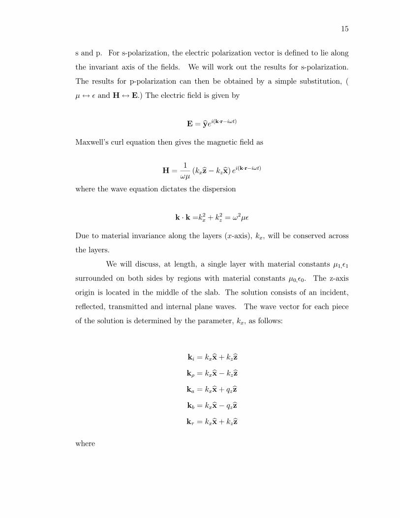
s and p. For s-polarization, the electric polarization vector is defined to lie along
the invariant axis of the fields. We will work out the results for s-polarization.
The results for p-polarization can then be obtained by a simple substitution, (
µ↔ ² and H↔ E.) The electric field is given by
E = byei(k·r−iωt)Maxwell’s curl equation then gives the magnetic field as
H =1
ωµ(kxbz− kzbx) ei(k·r−iωt)
where the wave equation dictates the dispersion
k · k =k2x + k2z = ω2µ²
Due to material invariance along the layers (x-axis), kx, will be conserved across
the layers.
We will discuss, at length, a single layer with material constants µ1,²1
surrounded on both sides by regions with material constants µ0,²0. The z-axis
origin is located in the middle of the slab. The solution consists of an incident,
reflected, transmitted and internal plane waves. The wave vector for each piece
of the solution is determined by the parameter, kx, as follows:
ki = kxbx+ kzbzkρ = kxbx− kzbzka = kxbx+ qzbzkb = kxbx− qzbzkτ = kxbx+ kzbz
where

16
x
yz
- d /2 d /20
a
b
i
ρ
τ
Ι Ι Ι Ι Ι Ιµ 0 , ε 0 µ 0 , ε 0µ 1 , ε 1
Figure II.2: Labeling conventions for boundary value problem.

17
kz =qk20 − k2x
qz =qµ²k20 − k2x
k20 = ω2µ0²0
µ =µ1µ0
² =²1²0
We desire the incident and transmitted wave to propagate or decay in the positive
z direction and the reflected wave to propagate or decay in the minus z direction.
These conditions are all met if we choose a branch of the square root for kz that
yields positive, real values for positive, real arguments and positive, imaginary
values for negative, real arguments. The default branch used on most computer
systems satisfies the criteria. This is the routine choice always employed in reflec-
tion and transmission problems and has nothing to do with NIM. However, the
choice of branch for qz is not routine and has everything to do with NIM. Fortu-
nately, we need not make any a priori choice since both signs of qz appear in our
trial solution.
The transverse component of the electric field in the three regions (figure
II.2) with unknown coefficients is given
Ey=eikxxe−iωt
eikzz + ρe−ikzz
aeiqzz + be−iqzz
τeikzz
I
II
III
(II.1)
This function must be continuous. Matching at the boundaries gives the first two
equations needed to solve the system of four unknowns.
e−ikzd/2 + ρeikzd/2 = ae−iqzd/2 + beiqzd/2
aeiqzd/2 + be−iqzd/2 = τeikzd/2
The transverse component of the magnetic field is given by

18
Hx= −eikxx
ωµ1e−iωt
µkze
ikzz − ρµkze−ikzz
aqzeiqzz − bqze−iqzzτµkze
ikzz
I
II
III
Matching at the boundaries gives the second two equations required to solve for
the four unknown coefficients.
µkze−ikzd/2 − ρµkze
ikzd/2 = aqze−iqzd/2 − bqzeiqzd/2
aqzeiqzd/2 − bqze−iqzd/2 = τµkze
ikzd/2
Solving the system of four equations yields the coefficients
τ = e−ikzd4µqzkzδ−1 (II.3a)
ρ = e−ikzd(qz + µkz)(qz − µkz)(eiqzd − e−iqzd)δ−1 (II.3b)
a = e−ikzd/22µkz(qz + µkz)e−iqzd/2δ−1 (II.3c)
b = e−ikzd/22µkz(qz − µkz)eiqzd/2δ−1 (II.3d)
where
δ ≡ (qz + µkz)2e−iqzd − (qz − µkz)2eiqzd (II.4)
The coefficients have definite symmetry with respect to qz
δ(−qz) = −δ(qz)τ(−qz) = τ(qz)
ρ(−qz) = ρ(qz)
a(−qz) = b(qz)
The symmetry of the these coefficients implies that the solution is invariant with
respect to choice of branch for the square root used to compute qz.

19
There is a resonant mode whenever δ = 0. This condition occurs when
e2iqzdµqz − µkzqz + µkz
¶2= 1 (II.5)
Note that when µ = ² = −1,this condition can never be satisfied, but wheneverthere is a deviation from this value, resonant modes occur. This condition has an
intuitive interpretation if one compares the above with the coefficient for single
interface reflection going from region II material to region I/III material.
ρ1 =qz − µkzqz + µkz
Then equation II.5 becomes
(eiqzdρ1)2 = 1
and the resonance condition says that one round trip within the slab returns the
plane wave to its original magnitude and phase. Thus the multiply reflected
waves within the slab constructively interfere with each other. It is worth noting
that if µ = ² = −1 exactly, then qz = kz, ρ1 is divergent, and there will be no
resonance for any finite value of qz. Taking the square root
eiqzdρ1 = ±1 (II.6)
we see that the two types of solutions are possible. For the plus sign, a one
way trip across the slab returns the plane wave to its original phase, yielding a
symmetric mode. For the minus sign a one way trip across the slab results in a π
phase shift, yielding an asymmetric mode. These slab modes can be decomposed
into symmetrically and anti-symmetrically coupled surface plasmons. Plasmons
are treated thoroughly in Ruppin[13], where equivalent forms of equation II.6 are
used
µkz + qz tanhqzd
2i= 0 (II.7)
µkz + qz cothqzd
2i= 0 (II.8)

20
Equation II.7 has solutions that are symmetric modes and equation II.8 has solu-
tions that are antisymmetric modes.
The k-space transfer function is defined as the ratio of the total field, Ey,
at some position, z1, to the incident field, Eyi, at some other position, z0 for a
given transverse wave vector, kx. z0 must lie in region I where the incident field
is defined. The transfer function depends implicitly on kx through kz and qz.
Tkx(z0, z1) ≡Ey(z1)
Eyi(z0)
The transfer function is given by
T(z0, z1) = δ−1
eikz(z1−z0) + (qz + µkz)(qz − µkz)(eiqzd − e−iqzd)e−ikz(z1+z0+d)
2µkze−ikz(z0+d/2) £(qz + µkz)e−iqz(d/2−z1) + (qz − µkz)eiqz(d/2−z1)¤
4µqzkzeikz(z1−z0−d)
I
II
III
(II.9)
Special Cases
When the material constants are both unity, µ = ² = 1, it is easy to show
that the transfer function reduces to
Tkx(z0, z1)=eikz(z1−z0)
which is the correct transfer function for a plane wave in free space.
For the perfect lens, µ = ² = −1, the electric field reduces to
Ey=eikxx
eikzz
e−ikz(z+d)
eikz(z−2d)
I
II
III
It is worth noting that, though no a priori choice was made for the wave vector
in the slab, only the −kz solution is present. This is the solution with negativephase velocity for propagating wave vectors and exponential growth behavior for

21
Figure II.3: Location of focii. The two focii occur at the locations marked z1.
The source is at z0.
evanescent wave vectors. The electric field is, of course, continuous and the transfer
function is given by
Tkx(z0, z1)=
eikz(z1−z0)
e−ikz(z1+z0+d)
eikz(z1−z0−2d)
z1 ∈ Iz1 ∈ IIz1 ∈ III
If z0 is within distance d of the slab (−3d/2 ≤ z0 ≤ −d/2) then
Tkx(z0, z0 + 2d) = 1
Tkx(z0,−z0 − d) = 1
This is perfect focusing of the z-plane at z0 onto a z-plane in region III and also a
plane in region II within the slab. The locations of these foci are shown diagram-
matically in figure II.3.

22
II.E Image Resolution: Approximate Analytical Results
Based on the transfer function derived above, it is possible to develop
a useful approximate analytical expression for material parameter deviation vs.
image resolution. The transfer function for the ideal object to image distance is
Tkx(z0, z0 + 2d) =4µqzkze
ikzd
(qz + µkz)2 e−iqzd − (qz − µkz)2 eiqzd
The exponential in the numerator arises from translation outside the slab. The
exponentials in the denominator arise from the solutions inside the slab. If µ =
² = −1 then qz = ±kz and one of the terms in the denominator is nulled out.The remaining term exactly cancels the numerator and we have perfect focusing.
If we do not have µ = ² = −1 then both terms are non-zero. An approximatecondition for marginal focusing occurs when the two terms have equal magnitude.
This condition is ¯qz + µkzqz − µkz
¯=¯eiqzd
¯This is the equation we will use to obtain an expression for the resolution. We
define the following measure of resolution
R ≡ |kx|k0
=λ0λx
This is just the number of spatial variations per free space wavelength. We wish
to find an approximation in the regime where this resolution is significantly greater
than one. This is the regime unavailable to conventional optics. We begin by
approximating qz and kz in this limit
qz ≈ i |kx|"1− 1
2µε
µk0kx
¶2#
kz ≈ i |kx|"1− 1
2
µk0kx
¶2#

23
The rational expression above becomes
qz + µkzqz − µkz ≈
(µ+ 1)− 12µ (ε+ 1)
³k0kx
´2(1− µ) + 1
2µ (1− ε)
³k0kx
´2If we deviate from the ideal permeability by a small amount µ = −1 + δµ with
² = −1 then we obtainqz + µkzqz − µkz ≈
1
2δµ
Similarly for a ² = −1 + δ² and µ = −1 we findqz + µkzqz − µkz ≈
1
4δε
µk0kx
¶2We use a zeroth order approximation for qz where it appears in the exponential
eiqzd ≈ e−|kx|d = e−Rk0d
and finally obtain
|δµ| = 2e−Rk0d (II.10a)
|δε| = 4R2e−Rk0d (II.10b)
These expression give the allowed parameter deviation from minus one to obtain
spatial resolution R. The allowable deviation is also strongly dependent on k0d,
the phase advance of a free space wave across the slab thickness d. Note that
the allowable deviation in the permittivity is greater than that allowed in the
permeability by the large factor 2R2. These roles are reversed for p-polarization.
The expression for δµ can be inverted to an explicit expression for the
resolution.
R = − lnµ |δµ|2
¶1
k0d(II.11)
The validity of these approximate expression for the resolution enhance-
ment is supported by comparing Eq. II.11 with Figure II.5. For example, for a
deviation of δµ = 0.005, the numerically computed transfer function has a limiting
resonance at kx/k0 ∼ 9.5, which is the same value predicted by Eq. II.11.

24
The dependence of the resolution enhancement R on the deviation from
the perfect lens condition is critical. The factor k0d dominates the behavior of
the resolution, the logarithm term being a relatively weakly varying function. For
example, if k0d2π= 1, we find that to achieve an R of 10, |δµ| must be less than
10−27! However, for k0d2π= 0.1, δµ can vary by as much as 0.004 to achieve the same
resolution enhancement. Similar deviations in either the real or the imaginary part
of the permeability will result in approximately the same resolution, although the
slab resonances occur only when the deviation occurs in the real part.
II.F Source Object
The source object is not literally a material object. Creating a focused
image of an object is the recreation, at some distance from the object, of the fields
that were produced or reflected by the object. So in the context of image formation,
the object is defined by the fields it produces. In our two dimensional geometry,
an object is a field distribution at an x-y plane, the object plane, at some z-axis
location, z0. An image is said to be formed if this same x-y field distribution is
recreated at some other location, z, the image plane.
Since we have chosen the y-axis to be homogenous, an x-y plane field
distribution is actually one dimensional. This one dimensional distribution can be
expanded in a one dimensional Fourier series.
Eyi(z0bz+ xbx) =Xkx
ckxeikxx
Each Fourier coefficient determines the phase and magnitude of a plane wave as
it passes through the object plane. The wave vector of this plane wave has x
component, kx, the transform variable, and z component, kz, determined from
equation ??. The coefficients are determined by the usual integral.
ckx =1
a
Z a/2
−a/2Eyi(z0bz+ xbx)e−ikxxdx

25
The periodicity, a, determines the kx interval as discussed in the next section. The
field distribution at any z plane is determined using Tkx to transfer the Fourier
coefficients to that plane.
Ey(zbz+ xbx) =Xkx
ckxTkx(z0, z)eikxx
II.G k-Space Mesh
The range of values of kx used for the above expansions is critical to the
accuracy of the solutions. A choice must be made for both the maximum value
of transverse wave vector, kxmax, and the spacing, dkx. These values cannot be
solely based on the requirements of accurately decomposing the source, ckx. When
transforming back to the spatial basis, the product ckxTkx appears in the inverse
transform. The k-space mesh must be adequate to represent all features of this
product. The transfer function Tkx(z0, z) can have resonances in kx which are quite
strong and narrow. These resonances can necessitate values of kxmax and dkx that
are larger and smaller respectively than would have been anticipated from just the
source spectrum, ckx. In fact for lossless media the resonance peaks are arbitrarily
sharp. Mesh refinement will never lead to image convergence. When it was desired
to isolate the effects of deviation of the real part of the material properties from
minus one, a small imaginary part was also added. This imaginary part was chosen
to be two orders of magnitude smaller than the deviation of the real part. This
small imaginary part is always smaller than what is realizable in a real material.
Another consideration for the k-space mesh is the periodicity. The wave
vector component spacing, dkx, determines the periodicity of the field patterns in
the x direction. The spatial period, a, is given by
a =2π
dkx
One may wish to require the local fields in the region of interest to be isolated.
For example, a slit source decomposed on a discrete mesh is actually an array of

26
slits separated by distance a. If we want to simulate the results for a single slit,
we want the fields from neighboring slits to be negligible in the region of interest.
To model the fields in the region within λ of a slit narrow slit, it is more than
sufficient if the neighboring slits are ten λ away. Then dkx =2π10λ. Typically this
is not as restrictive a requirement as representing resonance peaks in the transfer
function.
The approach used for determining the k-space mesh in this paper was to
check for convergence of the spatial fields. The value of kxmax (dkx) was sequentially
doubled (halved) until the change in the spatial field pattern fell below some small
threshold. In some cases this led to meshes in excess of 100K components.
II.H Image Resolution: Numerical Results
In this paper we explore eight different deviations from the ideal, µ =
² = −1, material properties. Each of the two material properties may deviatefrom minus one in four directions in the complex plain, figure II.4. Each of these
deviations gives somewhat different behavior. The behavior due to each of these
deviations was modeled using a thin slab of thickness d = λ/10, and an image to
object plane distance of 2d. The deviations modeled were logarithmically spaced
since the focusing properties scale as the log of the deviation (Eq. II.11.) Also,
the deviations modeled for ² were much larger than those for µ. This was done
to obtain a similar range of image resolutions for both parameters. As seen from
Eq. II.10, resolution is much more sensitive to µ than ² for s-polarization.
II.H.1 transfer function
Real Deviations
For non-matched material properties the transfer function displays sharp
peaks corresponding to resonances of the slab. This is seen in the first and third
panes of figures II.5 and II.6. These resonances, whose positions are given by

27
Figure II.4: Values of µ and ² simulated are shown in the complex plane. For
each value of µ and ², the transfer function and a real space image have been
calculated. Positive real deviations lead to symmetric modes and negative real
deviation lead to antisymmetric modes. µ deviations are shown in figure II.5 and
II.7 ε deviations in figures II.6 and II.8.

28
0 2 4 6 8 1 0 1 2 1 4
0 .1
1
1 0
1 0 0
k x / k 0
T(z
0,z
0+
2d
)
µ
µ
µ
µ
Figure II.5: The transfer function of the slab. In this and subsequent figures
the parameter that deviates from -1 is indcated in the upper right corner. The
direction of the deviation in the complex plane is indicated by an arrow. Lighter
shading of the line indicates larger deviation. The dashed line is the largest
deviation that can still resolve λ/10 features.

29
0 2 4 6 8 1 0 1 2 1 4
0 .1
1
1 0
1 0 0
k x / k 0
T(z
0,z
0+
2d
)
ε
ε
ε
ε
Figure II.6: The solid circles mark the points for which z field dependence is
shown. Circles in the top pane correspond to figure II.11 and circles in third pane
correspond to figure II.12.

30
- -x / 0
Figure II.7: Intensity of object and image focused by slab. The object is two
square peaks of unit intensity, width λ/100 and separation λ/10.

31
- -
Figure II.8: Intensity of object and image focused by slab. The object is two
square peaks of unit intensity, width λ/100 and separation λ/10.

32
Figure II.9: Resonance merge. The dashed line in the upper two panes is for the
value of µ that merges the two resonances. The bottom pane shows the center,
(x = 0), intensity versus µ. This intensity peaks at the merge, µ = −0.45.

33
Figure II.10: Resonance merge. The dashed line in the upper two panes is for
the value of ² that merges the two resonances. The bottom pane shows the center,
(x = 0), intensity versus ². This intensity peaks at the merge, ² = 3.45.

34
Figure II.11: Z dependence of the electric field excited by a unit plane wave of the
specified transverse wave vector, kx. The slab is delineated by the vertical grey
lines. The solid line is for µ = −1, ² = 1, and the dashed line is for µ = ² = −1.The phase is indicated by shading as shown in the legend.

35
Figure II.12: Z dependence of the electric field excited by a unit plane wave of the
specified transverse wave vector, kx. The slab is delineated by the vertical grey
lines. The solid line is for µ = −1, ² = −3, and the dashed line is for µ = ² = −1.The phase is indicated by shading as shown in the legend.

36
equation II.5, are modes of the system that can exist in the absence of excitation.
As the deviations are made smaller the resonance shifts to larger values of kx until,
at µ = ² = −1, the resonance has effectively shifted to infinity. In this case, thetail of the resonance gives the required gain within the slab to exactly compensate
for the decay of the evanescent waves outside the slab yielding a transfer function
of unity. For finite deviations from µ = ² = −1, the position of the resonancedetermines the maximum resolution of the slab. Beyond the resonance, the transfer
function decays exponentially
|Tkx| ∼ e−2kxd
The resonance condition, equation II.5, derived by setting the denomi-
nator of the transfer function to zero, predicts two resonances for real deviations
of the material parameters. One is near kx = k0, which is the boundary between
propagating and evanescent waves. The other, at a larger kx value, marks the up-
per end of the pass band of the transfer function. For negative material property
deviations (third pane of the figures), the lower resonance is symmetric and the
upper resonance is antisymmetric. However, for the lower, symmetric mode, the
zero in the denominator is cancelled by a zero in the numerator and no resonance
is observed in the transfer function.
For positive deviations of the material properties this does not occur and
both resonance peaks are evident in the transfer function (top pane of the figures).
Both of these modes are symmetric. Increasing the deviation causes the location
of the upper resonance to shift down and the lower resonance to shift up. There
is a special value of the material properties for which the two resonances merge.
For deviations of µ this value is µ = −0.45 as seen in figure II.9. For deviations of², the insensitive parameter, this special value occurs at a much larger deviation,
² = 3.45, figure II.10. When the resonances are coincident there exists a doubly
degenerate mode with strong gain over a wide band.

37
Imaginary Deviations
The deviations in the plus and minus imaginary direction yield materials
with loss or gain respectively. For positive deviations, no resonances are observed
(second pane of figures II.5 and II.6.) For negative deviations there is a bipolar peak
near k0, and the transfer function has values greater than one in the propagating
range, kx/k0 < 1, (fourth pane in the figures.) This requires an active material
with gain since propagating waves carry energy.
II.H.2 Spatial Images
The results of imaging a two “slit” source object are shown in figures II.7
and II.8. The slit spacing is λ/10. The individual slits have a width of λ/100
, and unit intensity. The image intensity curve was generated using the transfer
functions. In each graph the worst, (most deviant), transfer function that still
resolved the object is shown dashed. This particular configuration has a focusing
resolution of, ∼ λ/10, the slit spacing. The corresponding curve in the transfer
function plots is also dashed. The dashed curve in the transfer function has a band
limiting resonant peak at kx/k0 ∼ 8. This resolution is well beyond diffraction
limited optics, which can at best resolve images of λ/4. A desired resolution of
λ/10 permits only very small deviations of the sensitive parameter, µ, on the
order of one percent. The insensitive parameter may have rather large deviations
extending even to positive real values. The criteria used for image resolution is
as follows. The image must posses two peaks at locations consistent with the
object, and the intensity of these peaks must be greater than any other peaks in
the image, in particular they must be greater than the center peak. This criteria
gives reasonable agreement with equation II.11.
The images formed by a slab, with properties near the resonance peak
merge values, possess central peaks with large intensities. In fact the intensity of
the peak increases with increasing property deviation up to the merge point. The
third pane of figures II.9 and II.10 show the intensity of this peak as a function

38
of the material parameter. The case of epsilon deviation has a particularly large
image intensity. At the peak the intensity is more than an order of magnitude
larger than at any other value of the parameters.
II.H.3 Z Field Dependence
In figures II.11 and II.12 the z dependence of the electric field is shown
with an excitation of a unit plane wave. For plane wave excitation, the magnitude
of the electric field has no dependence on x as is clearly shown in equation II.1 and
the y axis was chosen to be homogenous, therefore the z dependence is a complete
description of the field. The material parameters chosen here are the largest ²
deviations that still permitted λ/10 image resolution, µ = −1 and ² = 1,−3. Forreference a perfect lens, µ = ² = −1, is shown also shown, (dashed). kx values werechosen to demonstrate the field behavior in the propagation range, evanescent pass
band, resonant peaks and beyond the pass band. In figure II.11, there are two
values of kx that are resonant shown in panes 2 and 4. The resonant fields are
large, symmetric in z, and π/2 out of phase with the desired response. These field
profiles are composed of two symmetrically coupled surface plasmon modes. The
surface plasmons in pane 4 are more strongly coupled than in pane 2. In the pass
band, pane 3, and the propagation range, pane 5, there is fair agreement with the
perfect lens, both in magnitude and phase. Beyond the pass band, pane 1, the
field is greater on the front surface of the slab than on the far surface, opposite to
what is required for super lensing. One can see the characteristic π phase shift of
the response when going through a resonance, panes 1-3.
Similar results are seen in figure II.12 except that only one resonance
is observed, and the mode is antisymmetric in z, composed of antisymmetrically
coupled surface plasmons.

39
Figure II.13: Geomtric arrangement of aperature slab.
II.I Aperture
Ey (x, z1) = A (x)F−1©eikz(z1−z0)F Ey (x, z0)
ªEy (x, z2) = F−1 T (z1, z2)F Ey (x, z1)Ey (x, z3) = F−1
©eikz(z3−z2)F A (x)Ey (x, z2)
ªA (x) =
1 |x| < A0/20 |x| ≥ A0/2
II.J Conclusion
The result of sub-wavelength focusing can be obtained using nothing but
Maxwell’s equations in a slab of NIM with standard boundary conditions enforced

40
Figure II.14: Image plane field for aperatured slab.
outside the slab. Materials with negative dielectric constants, (metals and plas-
mas), are familiar, and materials with negative permeability have been recently
demonstrated. Since Maxwell’s equations are not being called into question, these
results are on firm ground. Sub wavelength focusing is possible. It is however, dif-
ficult. Even for the case of a thin slab with minimal working distance, as explored
in this article, focusing resolution is very sensitive to at least one of the electro-
magnetic properties. In this case there is significant freedom in the other property
including its loss characteristics and the choice of polarization gives control over
which property is sensitive. The physical mechanism that limits the resolution
for real deviations of the material properties, is the excitation of slab resonance
modes. These modes mark the resolution cutoff of the transfer function.

41
II.K Acknowledgement
This chapter, in full, will be submitted for publication, with authors D.
Schurig, D. R. Smith, S. Schultz, S. A. Ramakrishna, J. B. Pendry.
II.L Material Parameters Simulated
µ ²−0.999 + 0.00001i −1−0.998 + 0.00002i −1−0.995 + 0.00005i −1−0.99 + 0.0001i −1−0.98 + 0.0002i −1−0.95 + 0.0005i −1−0.9 + 0.001i −1−0.8 + 0.002i −1−0.6 + 0.004i −1−0.3 + 0.007i −1µ ²−1 + 0.001i −1−1 + 0.002i −1−1 + 0.005i −1−1 + 0.01i −1−1 + 0.02i −1−1 + 0.05i −1−1 + 0.1i −1−1 + 0.2i −1−1 + 0.5i −1−1 + i −1µ ²−1.001 + 0.00001i −1−1.002 + 0.00002i −1−1.005 + 0.00005i −1−1.01 + 0.0001i −1−1.02 + 0.0002i −1−1.05 + 0.0005i −1−1.1 + 0.001i −1−1.2 + 0.002i −1−1.5 + 0.005i −1−2 + 0.01i −1−3 + 0.02i −1

42
µ ²−1− 0.001i −1−1− 0.002i −1−1− 0.005i −1−1− 0.01i −1−1− 0.02i −1−1− 0.05i −1−1− 0.1i −1−1− 0.2i −1−1− 0.5i −1−1− i −1µ ²−1 −0.9 + 0.001i−1 −0.8 + 0.002i−1 −0.5 + 0.005i−1 0.01i−1 1 + 0.02i−1 4 + 0.05i−1 9 + 0.1i
µ ²−1 −1 + 0.1i−1 −1 + 0.2i−1 −1 + 0.5i−1 −1 + i−1 −1 + 2i−1 −1 + 5i−1 −1 + 10iµ ²−1 −1.1 + 0.001i−1 −1.2 + 0.002i−1 −1.5 + 0.005i−1 −2 + 0.01i−1 −3 + 0.02i−1 −6 + 0.05i−1 −11 + 0.1i−1 −21 + 0.2i−1 −51 + 0.5i

43
µ ²−1 −1− 0.1i−1 −1− 0.2i−1 −1− 0.5i−1 −1− i−1 −1− 2i−1 −1− 5i, −1 −1− 10i

Chapter III
Electromagnetic Wave
Propagation in Media with
Indefinite Permittivity and
Permeability Tensors
III.A Abstract
We study the behavior of wave propagation in materials for which not
all of the principle elements of the permeability and permittivity tensors have the
same sign. These tensors are neither positive nor negative definite. We find that a
wide variety of effects can be realized in such media, including negative refraction,
near-field focusing and high impedance surface reflection. In particular a bilayer of
these materials can transfer a field distribution from one side to the other, including
near-fields, without requiring internal exponentially growing waves.
III.B Introduction
The range of available electromagnetic material properties has been broad-
ened by recent developments in structured media, notably Photonic Band Gap ma-
44

45
terials and metamaterials. These media have allowed the realization of solutions
to Maxwell’s equations not available in naturally occurring materials, fueling the
discovery of new physical phenomena and the development of devices. Photonic
crystals, for example, have been utilized to modify the radiative density of states
associated with nearby electromagnetic sources. Optical effects such as superradi-
ance [23], enhanced or inhibited spontaneous emission [24], ultrarefraction [25] and
even negative refraction [10, 11] have been predicted for various photonic lattice
configurations.
The propagation characteristics of photonic lattices, while unique, are
not conveniently expressed in a compact manner, and it is usually necessary to
compute photonic band structure diagrams to deduce wave propagation behavior.
By contrast, when the size and spacing of the constituent elements composing a
medium are much smaller than the wavelength of interest, the composite can be
treated as a continuous material–or metamaterial, with a permittivity tensor (ε)
and a permeability tensor (µ) [26]. This reduction of complexity simplifies the
discussion of wave phenomena, without requiring undue attention to the detailed
responding fields and currents characterizing the scattering elements. Typically,
ε and µ are positive definite, and the associated propagation behavior has been
well-studied, including, more recently, chirality and bianisotropy [27, 28].
In 2000, it was shown experimentally that a metamaterial composed of
periodically positioned scattering elements, all conductors, could be interpreted
as having simultaneously a negative effective permittivity and a negative effec-
tive permeability [1]. Such a medium had been previously shown by Veselago
to be consistent with Maxwell’s equations [3], but had never been demonstrated
in a naturally occurring material or compound. A medium with simultaneously
isotropic and negative ε and µ supports propagating solutions whose phase and
group velocities are antiparallel. Equivalently, such a material can be rigorously
described as having a negative index of refraction[4]. An experimental observation
of negative refraction was achieved using a metamaterial composed of wires and

46
split ring resonators deposited lithographically on circuit board material [2].
The prospect of negative refractive materials has generated considerable
interest, as this simply stated material condition suggests the possibility of extraor-
dinary wave propagation phenomena, including near-field focusing. Yet, negative
refraction is not confined to materials with negative definite ε and µ, but can also
be observed in materials with indefinite ε and µ tensors. Lindell et al. [29] have
shown that negative refraction can occur in uniaxially anisotropic media, and that
such media are characterized by hyperbolic dispersion curves. We refer here to
such materials as indefinite media for brevity. After a general discussion of the
possible classes of indefinite media, we analyze the reflection and refraction prop-
erties for several configurations that may be relevant for unique applications. The
components used to demonstrate the previous negative index metamaterials are
appropriate building blocks for the classes of materials to be discussed here.
III.C Media
To simplify the following analysis, we assume a material whose anisotropic
permittivity and permeability tensors are simultaneously diagonalizable, having
the form
ε =
εx 0 0
0 εy 0
0 0 εz
µ =
µx 0 0
0 µy 0
0 0 µz
. (III.1)
We are interested in the manner in which a plane wave interacts with an anisotropic
medium, in which not all of the diagonal components of the ε and µ tensors have
the same sign. To facilitate our analysis we consider an electromagnetic wave with
the polarization directed along the y-axis, or
E = byei(kxx+kzz−ωt). (III.2)
From the electromagnetic wave equation, we find the following dispersion relation:
k2z = εyµxω2
c2− µxµzk2x, (III.3)

47
where we consider the +z-axis to be the forward reference direction. The wave
vector has just one transverse component, kx. Using only real values of kx we
can expand any field distribution along the x direction using a Fourier series or
transform, so we will restrict our discussion to real valued kx, as is appropriate for
the consideration of reflection/refraction phenomena.
The sign of k2z determines the nature of the plane wave solutions. k2z > 0
corresponds to real valued kz and propagating solutions. k2z < 0 corresponds to
imaginary kz and exponentially growing or decaying (evanescent) solutions. The
value of kx for which k2z = 0 is referred to as the cutoff, kc. kc separates propagating
from evanescent solutions. Based on the type of solutions of Eq. III.3, we identify
four classes of media:
Always Evanescent εyµx < 0 µx/µz > 0Cutoff εyµx > 0 µx/µz > 0Anti-Cutoff εyµx < 0 µx/µz < 0Always Propagating εyµx > 0 µx/µz < 0
At a given frequency, we can visualize the dispersion by plotting values of kz versus
kx as shown in Fig. III.1. Waves in an always evanescent medium are evanescent
for any direction of propagation. Waves in a cutoff medium are propagating for
kx < kc, and evanescent for kx > kc. Examples of this medium class include
free space, and any medium with ε and µ tensors both positive or both negative
definite. diagonal permittivity and permeability elements. The other two classes
of media, anti-cutoff and always propagating, require indefinite material property
tensors and have hyperbolic dispersion. Waves in anti-cutoff media are evanescent
for kx < kc, and propagating for kx > kc. Waves in always propagating media
propagate for all kx[30].
We can examine the direction of energy flow for waves in indefinite media
by calculating the group velocity, vg ≡ ∇kω (k). Since negative material property

48
Figure III.1: Iso-frequency curves for different classes of media. The cutoff trans-
verse wave vector, kc, is indicated for the cutoff and anti-cutoff media. Solid lines
indicate real valued kz. Dashed lines indicate imaginary values.

49
components are necessarily dispersive, we must use a causal, dispersive response
function to represent them. For simplicity, we use the same, real-valued (lossless),
response function, ξ (ω), for all negative components of µ or ε. Positive components
are assumed non-dispersive. Also for simplicity, we choose unit magnitude for all
components. The slope of the response function is constrained by causality
ξ (ω0) = −1 ξ0 (ω0)ω0 ≥ 2 (III.4)
For the always propagating medium, then,
ε = µ =
ξ (ω) 0 0
0 ξ (ω) 0
0 0 1
(III.5)
The group velocity of a wave packet centered on a wave vector k = kxbx + kzbz isthen
vg = cf (kx)kxbx− kzbz
ω0/c(III.6)
where f (kx) is a dimensionless, positive, real scalar. Note that the group and
phase velocity form an obtuse angle of nearly 180 for small kx, and nearly 90 for
large kx. The direction of the group velocity is given for several other materials in
Fig. III.2.
III.D Refraction and Reflection
The unusual dispersive properties of indefinite media are manifest in re-
flection and refraction phenomena . We use k to indicate the plane wave vector
incident from the free space side of the interface, and q to indicate the transmit-
ted wave vector, inside the indefinite medium. The surface is assumed normal to
the z-axis resulting in translational symmetry in the x and y directions and thus
kx = qx.
The nature of refraction into an indefinite medium is illustrated in Fig.
III.3 for an always propagating material. The wave vector and group velocity of

50
Figure III.2: Each medium class has two sub-types, positive and negative. The
sub-type indicates the direction of refraction, or equivalently, the sign of the z-
component of the group velocity relative to the wave vector. Negation of both µ
and ε switches the sub-type. (For ease of illustration, the tensors in this table
and those used for all specific calculations and plots in this article have elements
of unit magnitude.)

51
Figure III.3: Refraction from free space (blue) into negative, (green) and positive,
(red) always propagating media. Only the real parts of the dispersion curves are
shown. The free space curve is black and the always propagating medium is gray.
The white, construction lines indicate the conservation of transverse wave vector,
etc. The lengths of the group velocity vectors are not shown to scale.

52
the incident wave are parallel and the wave vector lies on the free space dispersion
curve. The direction for the refracted wave is uniquely determined by three con-
straints: 1. The transverse component of the wave vector is conserved, kx = qx.
2. The z-component of the group velocity must maintain its sign (for energy con-
servation.) 3. The group and phase velocity form an angle given by the group
velocity expression, Eq. (III.6). We see that the negative always propagating ma-
terial exhibits negative refraction of the wave vector and positive refraction of the
group velocity. The positive always propagating material exhibits just the opposite
behavior. Refraction into other classes of materials can be similarly characterized,
and the refraction directions are shown in Fig. III.2.
The reflection properties of indefinite media display interesting behavior,
illustrated here for positive anti-cutoff material. The reflection coefficient is given
by
ρ =µxkz − qzµxkz + qz
(III.7)
For unit magnitude anti-cutoff material we have, from Eq. (III.3),
q2z = −ω2
c2+ k2x = −k2z (III.8)
Thus qz = ±ikz. The correct sign, +, is determined from a construct similar to
Fig. III.3. We then have
ρ =1− i1 + i
= −i (III.9)
The magnitude of the reflection coefficient is unity, with a phase of -90 for prop-
agating modes of all incident angles. An electric dipole antenna placed λ/8 away
from the surface would thus be enhanced by interaction with the mirror surface.
Customized reflecting surfaces are of practical interest, as they enhance the effi-
ciency of nearby antennas, while at the same time providing shielding [31, 32]. In
this case, the uniformity of the reflection coefficient over all angles of incidence may
be advantageous. Furthermore, surface modes, which require evanescent solutions
on both sides of the interface, are not supported on this interface. Fig. III.1 shows

53
no overlap of evanescent solutions (dashed line) between cutoff and anti-cutoff
media (with the same cutoff wave vector.)
III.E Layered Media: Focusing
Amotivating factor in the recent metamaterials effort has been the prospect
of near-field focusing, as introduced by Pendry, who showed theoretically that a
planar slab with isotropic ε = µ = −1, and thickness, 2d, could act as a lens withresolution well beyond the diffraction limit. A field source positioned a distance
d from the first interface will form an image a distance d away from the other
interface. Not only are the propagating components of the source refocused, but
the decay of the evanescent components is reversed through the material, the net
result being that the image exactly reproduces the source fields, even if the source
field spatial distribution is much less than the wavelength. It is difficult, how-
ever, to realize significant sub-wavelength resolution in practice, as the required
exponential growth of the large kx field components across the negative index lens
leads to extremely large field ratios[7, 33]. Sensitivity to material loss and other
factors can significantly limit the sub-wavelength resolution. A proposed scheme
to reduce this sensitivity is to section the planar lens into numerous separated
subsections[34]. In the limit of a large number of very thin layers, the transverse
and longitudinal effective material parameters exhibit extreme anisotropy, sug-
gesting that anisotropic materials may be inherently advantageous for near-field
focusing.
While it is not possible to focus near-fields with a single layer of an indef-
inite medium, it is possible to compensate for the dispersive effects of a negative
always propagating layer with a positive always propagating layer. Fig. III.3 indi-
cates that for the same incident plane wave, the z-component of the transmitted
wave vector, qz, is equal and opposite for these two materials. Combining equal
lengths of these materials results in a composite indefinite medium with unit trans-
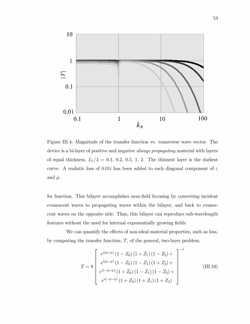
54
Figure III.4: Magnitude of the transfer function vs. transverse wave vector. The
device is a bi-layer of positive and negative always propagating material with layers
of equal thickness, L1/λ = 0.1, 0.2, 0.5, 1, 2. The thinnest layer is the darkest
curve. A realistic loss of 0.01i has been added to each diagonal component of ε
and µ.
fer function. This bilayer accomplishes near-field focusing by converting incident
evanescent waves to propagating waves within the bilayer, and back to evanes-
cent waves on the opposite side. Thus, this bilayer can reproduce sub-wavelength
features without the need for internal exponentially growing fields.
We can quantify the effects of non-ideal material properties, such as loss,
by computing the transfer function, T , of the general, two-layer problem.
T = 8
ei(φ+ψ) (1− Z0) (1 + Z1) (1− Z2)+ei(φ−ψ) (1− Z0) (1− Z1) (1 + Z2)+ei(−φ+ψ) (1 + Z0) (1− Z1) (1− Z2)+ei(−φ−ψ) (1 + Z0) (1 + Z1) (1 + Z2)
−1
(III.10)

55
where the impedances are defined as
Z0 =qz1µx1kz
, Z1 =µx1µx2
qz2qz1, Z2 = µx2
kzqz2. (III.11)
and the individual layer phase advance angles are defined as
φ ≡ qz1L1 ψ ≡ qz2L2.
L1 is the thickness of the first layer and L2 is the thickness of the second layer. For
ideal positive always propagating and negative always propagating layers of equal
thickness, the transfer function is unity for all incident plane waves. The transfer
function with some realistic loss added is shown in Fig III.4.
A proposed implementation is shown in Fig. III.5. The top and bottom
structures will focus S-polarized and P-polarized waves respectively. Combining
the two structures results in a bilayer that focuses both polarizations and is x-
y isotropic. The materials are formed from split ring resonators and wires with
numerically and experimentally confirmed effective material properties [2]. Each
split ring resonator orientation implements negative permeability along a single
axis, as does each wire orientation for negative permittivity.
III.F Conclusion
We have begun to explore the properties of media with indefinite ε and
µ tensors. Indefinite media are governed by hyperbolic dispersion relations, previ-
ously found only in much more exotic situations, such as relativistic moving media
[28]. Consideration of layered structures has led to useful and interesting reflection
and refraction behavior, including a new mechanism for sub-diffraction focusing.
We note that neither the analysis nor the fabrication of these media is compli-
cated, and thus anticipate other researchers will quickly assimilate the principles
and design structures with unique and technologically relevant properties.

56
Figure III.5: Split ring resonators are shown in black. Wires are shown in gray.
Upper device: layer one has split ring resonators oriented in the x direction and
wires in the y direction, and layer two has split ring resonators in the z direction.
Lower device: layer one has split ring resonators oriented in the y direction and
wires in the x direction, and layer two has wires in the z direction.

57
III.G Acknowledgement
We thank Claudio Parazzoli (PhantomWorks, Boeing) for motivating this
work. This work was supported by DARPA through grants from ONR (Contract
No. N00014-00-1-0632) and AFOSR (Contract No. 78535A/416250/440000) and
a grant from AFOSR (Contract Number F49620-01-1-0440).
This chapter, in full, has been submitted for publication to Physical Re-
view Letters, with authors D. R. Smith and D. Schurig.

Chapter IV
Sub-Diffraction Focusing Using
Bilayers of Indefinite Media
IV.A Abstract
We analyze a new type of near field focusing device that consists of a
bilayer of media with indefinite electromagnetic material property tensors. The
dispersion of the media supports propagating waves for any transverse wave vector
which results in a weaker dependence of spatial bandwidth on media lossiness.
IV.B Introduction
Pendry’s theoretical demonstration that a layer of negative index media
could focus near as well as far fields and operate as a “perfect” lens has generated
a lot of interest [6, 35, 36, 37, 38, 33, 7, 5, 39]. Here we discuss near field focusing
in a broader context, and employing bilayers of a new class of media that are
anisotropic [40]. The devices proposed here belong to a general class of bilayers
that have compensating layers; the phase advance (or decay) across one layer is
equal and opposite to the phase advance (or decay) across the other layer. Pendry’s
“perfect” lens is a special case of a compensating bilayer. In this case the negative
index media compensates for free space, and thus the device has the nice feature
58

59
that it possesses free space working distance. To be compensating, one layer must
have normal components of the wave vector and group velocity of the same sign
and the other layer must have normal components of opposite sign. This ensures
that energy moving across the bilayer has opposite evolution in one layer relative
to the other.
The device to be discussed in this letter is a compensating bilayer that
employs a particular class of media we refer to as always propagating [40]. The
most unusual property of this medium is that it supports propagating waves for
all transverse wave vectors. Even waves that are evanescent in free space, when
incident on this medium, are converted to propagating waves. There are two
sub-classes of always propagating media that together can satisfy the requirements
for a compensating bilayer. The main advantage of using this medium is less
sensitivity to material lossiness. Bilayers that do not use an always propagating
medium, such as the Pendry lens, must support large growing field solutions that
are very sensitive to material loss[33, 37, 7].
Always propagating media are anisotropic, and in fact have both positive
and negative principle components in the electromagnetic property tensors, ε and
µ. Because these tensors are neither positive nor negative definite, we refer to this
medium as an indefinite medium [40].
IV.C Dispersion
To simplify the following analysis, we assume a material whose anisotropic
permittivity and permeability tensors are simultaneously diagonalizable, having
the form
ε =
εx 0 0
0 εy 0
0 0 εz
µ =µx 0 0
0 µy 0
0 0 µz
.

60
Consider an electromagnetic wave with the polarization directed along the y-axis,
E = byei(kxx+kzz−ωt).From the electromagnetic wave equation, we find the following dispersion relation:
k2z = εyµxω2
c2− µxµzk2x,
where we consider the +z-axis to be the forward reference direction. The wave
vector has just one transverse component, kx. Using only real values of kx we
can expand any field distribution along the x direction using a Fourier series or
transform, so we will restrict our discussion to real valued kx.
The sign of k2z determines the nature of the plane wave solutions. Pos-
itive k2z corresponds to real valued kz and propagating solutions. Negative k2z
corresponds to imaginary kz and exponentially growing and decaying (evanescent)
solutions. For the devices discussed in this paper we will consider materials that
are always propagating, that is kz real for all values of kx. These materials satisfy
εyµx > 0 andµxµz< 0
This requires material property tensors that have principle values that are not all
of the same sign. The dispersion is hyperbolic [29] with asymtotes of slope, m,
defined at large kx by
m ≡¯∂kz∂kx
¯=
¯kzkx
¯=
s¯µxµz
¯(IV.1)
As will be seen below, this slope is directly observable in spatial electric field
intensity patterns. The constant frequency dispersion is shown in Fig. IV.1. Note
that for all values of kx there are real values of kz. Since this curve is a constant
frequency contour the group velocity, vg = ∇kω (k), must be normal to the curve.From the figure one can see that at large kx, vg will also be normal to k. There
are two types of always propagating material that correspond to the two possible
directions of the group velocity. The simplest tensor forms for these two types are
given in Eq. (IV.6).

61
Figure IV.1: Hyperbolic dispersion found in always propagating media (black).
The asymtotic behavior is also shown (white.) Two wave vectors are shown that
have the same transverse component, kx. Both possible group velocity directions
are shown for each wave vector. The normal (z) component of k and vg can be
either of the same sign or opposite sign.
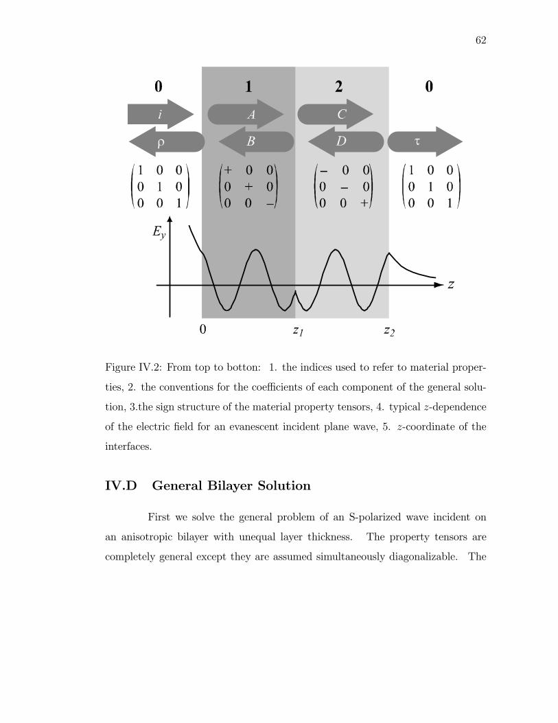
62
Figure IV.2: From top to botton: 1. the indices used to refer to material proper-
ties, 2. the conventions for the coefficients of each component of the general solu-
tion, 3.the sign structure of the material property tensors, 4. typical z-dependence
of the electric field for an evanescent incident plane wave, 5. z-coordinate of the
interfaces.
IV.D General Bilayer Solution
First we solve the general problem of an S-polarized wave incident on
an anisotropic bilayer with unequal layer thickness. The property tensors are
completely general except they are assumed simultaneously diagonalizable. The

63
general solution for the electric field with unknown coefficients is given by
Ey = ei(kxx−ωt)
eikzz + ρe−ikzz
Aeipzz +Be−ipzz
Ceiqzz +De−iqzz
τeikzz
z < 0
0 < z < z1
z1 < z < z2
z2 < z
The z-components of the wave vectors are
kz = ±qk20 − k2x (IV.2a)
pz = ±r
ε1yµ1xk20 −µ1xµ1zk2x (IV.2b)
qz = ±r
ε2yµ2xk20 −µ2xµ2zk2x (IV.2c)
where k0 = ω2/c2 and the material parameters are relative to free space. The
conventions for the material property subscripts and solution coefficients are shown
in Fig. IV.2. The general solution includes exponentials with both signs of pz and
qz so a choice of sign for these square roots is unnecessary. We choose the branch
of the square root for kz such that kz is either real and positive or imaginary and
positive. This ensures that the incident wave propagates toward the bilayer or
decays in the direction toward the bilayer (away from the source). The transverse
component (y) of the electric field is conserved across each of the three interfaces,
at z = 0, z = z1 and z = z2, yielding three equations. Similarly the transverse
component (x) of the magnetic field yields three more equations. The transverse
magnetic field component is given by
Hx = − 1ωei(kxx−ωt)
kz¡eikzz − ρe−ikzz
¢pzµ1x(Aeipzz −Be−ipzz)
qzµ2x(Ceiqzz −De−iqzz)kzτe
ikzz
z < 0
0 < z < z1
z1 < z < z2
z2 < z
The six boundary matching equations are solved for the six unknown coefficients:
ρ, A,B,C,D, τ . The transfer function from the front surface to the back surface

64
of the bilayer is given by the ratio of the transmitted electric field to the incident
electric field
T =Ey (z2)
Eyi (0)= τeikzz2
Inserting the value of τ from the solution of the system of six equations yields
T = 8
ei(φ+ψ) (1− Z0) (1 + Z1) (1− Z2)+ei(φ−ψ) (1− Z0) (1− Z1) (1 + Z2)+e−i(φ−ψ) (1 + Z0) (1− Z1) (1− Z2)+e−i(φ+ψ) (1 + Z0) (1 + Z1) (1 + Z2)
−1
(IV.3)
where the impedances are defined as
Z0 ≡ pzµ1xkz
Z1 ≡ µ1xqzµ2xpz
Z2 =µ2xkzqz
, (IV.4)
and the individual layer phase advance angles are defined as
φ ≡ pzz1 ψ ≡ qz (z2 − z1) . (IV.5)
To obtain a unit transfer function, T = 1, it is sufficient that
φ± ψ = 0 and 1∓ Z1 = 0.
These two conditions are equivalent to layer compensation as discussed above,
and the additional requirement of an impedance match between the layers.
IV.E Simplest Case
We examine the archtypical focusing bilayer. In this case (and all others
discussed in this paper), we will choose the ε and µ tensors equal to each other and
thus ensure that the focusing properties are independent of polarization. We also
choose these tensors to be x-y isotropic so that the focusing properties are indepen-
dent of the x-y orientation of the layers. This is the highest degree of symmetry

65
allowed for always propagating media. If we further choose unit magnitude for all
tensor components we have
ε1 = µ1 =
1 0 0
0 1 0
0 0 −1
ε2 = µ2 =
−1 0 0
0 −1 0
0 0 1
(IV.6)
In this case the layer thickness must be equal for focusing, z1 = z2 − z1 = d.
Plugging these values into Eq. (IV.2), (IV.3), (IV.4) and (IV.5), we find the
transfer function is unity for all incident plane waves, T = 1. The magnitude is
preserved and the phase advance across the bilayer is zero.
The internal field coefficients (A,B,C,D) are plotted in Fig. IV.3. Evanes-
cent incident waves (kx/k0 > 1) carry no energy, but on entering the bilayer are
converted to propagating waves. Since propagating waves do carry energy the
forward and backward coefficients must be equal; the standing wave ratio must be
and is unity.
Propagating incident waves, however, do transfer energy across the bi-
layer. We see in the figure that for propagating incident waves, (kx/k0 < 1),
the first layer, forward coefficient, |A|, is larger in magnitude than the backwardcoefficient, |B|. These rolls are reversed in the second layer, |D| > |C|. Whatwe have referred to as “forward” really means positive z-component of the wave
vector. This does not indicate the direction of energy flow which is given by the
group velocity. The z-component of the group velocity must be positive in both
layers to conserve energy across the interfaces. We can display the electric field
quite simply in the limit kx À k0.
Ey = ei(kxx−ωt)
e−kxz√2 cos [kxz + π/4]
√2 cos [kx (2d− z) + π/4]
e−kx(z−2d)
z < 0
0 < z < d
d < z < 2d
2d < z
we see that the internal field is indeed a standing wave, and is symmetric about
the center of the bilayer. This field pattern is shown in Fig. IV.2.

66
Figure IV.3: The magnitude of coefficients of the internal field components. For
values of kx > k0 (incident plane wave is evanescent) the forward and backward
components have equal magnitude. The magnitude approaches 1/√2 when kx À
k0.

67
IV.F Asymmetric Bilayers and Field Plots
We can relax the above symmetry to obtain some different behavior.
In the previous discussion the property tensor elements were all unit magnitude
leading to dispersion slope of one, as seen from Eq. (IV.1). We can introduce a
different slope, m, as follows
ε1 = µ1 =
m1 0 0
0 m1 0
0 0 −1/m1
ε2 = µ2 =
−m2 0 0
0 −m2 0
0 0 1/m2
Allowing the slope to differ in each layer we can still maintain a unit transfer
function, T = 1, if we adjust the thickness of the layers appropriately.
z2 − z1z1
=m1
m2
We have still maintained polarization independence and x-y isotropy. The internal
field for a bilayer with different slopes in each layer is shown in Fig. IV.4. The
incident field is a localized source composed of many kx components. This source
is equivalent to two narrow slits back illuminated by a uniform propagating plane
wave. The plane wave components interfere to form a field intensity pattern that
is localized in four beams, two for each slit. The beams diverge in the first layer
and converge in the second layer to reproduce the incident field pattern on the far
side. The plane waves that constructively interfere to form each beam have phase
fronts parallel to the beam, (i.e. the wave vector is perpendicular to the beam.)
The narrow slits yield a source which is dominated by large kx components. These
components lie well out on the asymtotes of the hyperbolic dispersion, so all of the
wave vectors point in just four directions, the four indicated in the plot. These

68
correspond to the positive and negative kx components in the source expansion
and the forward and backward components of the solution (A,B or C,D).
IV.G Lossy Media: Approximate Analytical Transfer Func-
tion
Lossy media is characterized by an imaginary component of the property
tensors. We will use a single parameter for the imaginary component of all the
principle elements of both ε and µ.
ε1 = µ1 =
m+ iγ 0 0
0 m+ iγ 0
0 0 −1/m+ iγ
ε2 = µ2 =
−m+ iγ 0 0
0 −m+ iγ 0
0 0 1/m+ iγ
For this analysis we will use layers of equal slope and thickness, z1 = z2 − z1 = d.Fig. IV.5 shows the effect of loss on the transfer function. Increasing loss limits the
kx bandwidth. We can obtain a simple analytical approximation for the transfer
function to see directly the trade-offs between bandwidth, slope, thickness and
loss. We will assume that the loss parameter is small compared to the real part
of the principle components of the material property tensors, γ ¿ 1/m,m. We
will also assume that kx À k0, limiting the range of validity of our approximate
transfer function to large kx. However, it will turn out that the approximate
transfer function will give a realistic value of one for small kx. In any case, we
usually wish to find the upper limit of the pass band which will occur at large kx
in most useful circumstances. If we evaluate the transfer function, Eq. (IV.3), to
zeroth order in γ for the impedance factors we obtain
T = sec (φ− ψ) .

69
Figure IV.4: Internal electric field intensity plot for a localized two slit source.
The four vector pairs in each layer indicate the only four orientations of internal
plane waves. Plane waves from positve kx components of the source are indicated
in white and negative in gray. The wave vectors are labeled with the solution
component to which they corresond. kA and kC have positve z-components and kB
and kD have negative z-components. The unmarked vector in each pair indicates
the direction of the group velocity for that plane wave direction. m1 = 1 and
m2 = 1/2.

70
Figure IV.5: The transfer function from the front surface to the back surface of
the bilayer. z1 = z2 − z1 = λ, m = 1/3 and ε00 = µ00 = .001, .002, .005, .01, .02,
.05, .1, from light to dark. For comparison, a single layer, isotropic near field lens
is shown dashed. The single layer has thickness, λ, and ε = µ = −1 + 0.001i.

71
If we then expand φ and ψ to first order, we obtain
T = sech£kxd
¡1 +m2
¢γ¤
This approximate transfer function has excellent agreement with the full expres-
sion, Eq. (IV.3), in the appropriate limits. In particular it accurately gives the
behavior at high kx values where the transfer function rolls off . The dependence
of bandwidth, ∆kx, on thickness, d, loss, γ, and slope, m, is given by
∆kxd¡1 +m2
¢γ ∼ 1 (IV.7)
Not surprisingly, larger bandwidth is obtained with thinner layers and smaller loss.
Less intuitive is the role of the slope, m; smaller slope gives larger bandwidth. In
Fig. IV.4 we observe that a smaller slope corresponds to beams that lie on a more
direct path through the layer. For fixed thickness, d, this means a shorter path.
One might suggest thatm = 0, with beams going straight through the layer, would
be the most desirable. However, our analysis is only valid formÀ γ. In addition,
since 1/m also appears as a principle component in the property tensors, there is
a practical limit to how small m can be. Arbitrarily large ε and µ components
are not realizable.
We note that Ramakrishnan and Pendry have proposed another device
that also has reduced sensitivity to loss compared to the single layer “perfect” lens
[34]. This device uses an infinite number of infinitesimally thin layers of isotropic,
negative index medium. We have found that this configuration gives the same
inverse relation between loss and bandwidth as Eq. (IV.7). This dependence is
markedly different from that of a single layer which has exponential dependence.
γ ∼ e−∆kxd
IV.H Conclusion
We have analyzed a new type of near field focusing device that consists
of a bilayer of always propagating media. This unusual media possesses indefinite

72
material property tensors. We have found the slope of the dispersion relation to
be a useful adjustable parameter that is directly observable in field intensity plots.
Internal standing waves are employed to transfer externally evanescent waves across
the device, and the dependence of spatial transfer function bandwidth on material
lossiness is much more favorable than in single layer, isotropic devices.
IV.I Acknowledgement
This chapter, in full, will be submitted for publication, with authors D.
Schurig and D. R. Smith.

Chapter V
Electromagnetic Spatial Filtering
Using Media with Negative
Properties
V.A Abstract
We show how bilayers of media with negative electromagnetic property
tensor elements can be used to construct low, high and band pass spatial filters.
These filters possess sharp adjustable roll offs and can operate in the near and far
field regimes to select specific spatial variation components or beam angles.
V.B Introduction
There has been a great deal of interest in the “perfect” lens[6, 35, 36, 37,
38, 33, 7, 5, 39]. Researchers have found that the parameter range for which the
“perfect” lens can focus near fields is quite limited[33, 37, 7]. In particular, it
has been found that the lens must be thin and the losses small to have a spatial
transfer function that operates significantly into the near field (evanescent) range.
Even with small losses a thick lens will have a transfer function that rolls off quite
steeply at the near/far field boundary. However, in the far field (propagating)
73

74
range the “perfect” lens is fairly robust, and a wide range of lens thickness and
material loss can be tolerated.
This article discusses the exploitation of this effect which can result in
a flat response for wave vectors in the propagating range and up to the evanes-
cent boundary followed by a strongly attenuated response. This is a desirable
characteristic of a spatial low pass filter. The “perfect” lens by itself would be of
limited usefulness because the filter cutoff is fixed at a specific wave vector, but it
is possible to tune this filter cutoff by employing compensating bilayers.
Compensating bilayers have the property that the phase advance (or de-
cay) across one layer is equal and opposite to the phase advance (or decay) across
the other layer. The “perfect” lens is a special case of a compensating bilayer.
In this case the negative index media compensates for free space, and thus the
device has the nice feature that it allows for free space working distance. To be
compensating, one layer must have normal components of the wave vector and
group velocity of the same sign and the other layer must have normal components
of opposite sign. This ensures that energy moving across the bilayer has opposite
evolution in one layer relative to the other.
Compensating bilayers can be composed of media with cutoffs that are
different from free space. The cutoff can be tuned to a value below the free space
cutoff, so the filter edge is in the propagating range. Then a bilayer can operate
as an angular selector. The cutoff can also be tuned to a value above the free
space cutoff to make a near field spatial filter.
Bilayers composed of isotropic media like the “perfect” lens can only
function as low pass filters, however another type of media, which we refer to as
anti-cutoff media, can be used to construct compensating bilayers that function as
high pass filters. Anti-cutoff media require anisotropic electromagnetic property
tensors that do not have principle components all of the same sign. These tensors
are neither positive nor negative definite, so we refer to these media as indefinite
media [40].

75
Band pass filters can also be realized as a four layer device composed of
two adjacent compensating bilayers. The high and low cutoffs can be adjusted
independently, and the two bilayers do not interfere with each other in the pass
band, where the reflection coefficient is small.
V.C Dispersion
To simplify the following analysis, we assume a material whose anisotropic
permittivity and permeability tensors are simultaneously diagonalizable, having
the form
ε =
εx 0 0
0 εy 0
0 0 εz
µ =µx 0 0
0 µy 0
0 0 µz
.Consider an electromagnetic wave with the polarization directed along the y-axis,
E = byei(kxx+kzz−ωt).From the electromagnetic wave equation, we find the following dispersion relation:
k2z = εyµxk20 −
µxµzk2x,
where k0 = ω/c and the material parameters are relative to free space. We consider
the +z-axis to be the forward reference direction. The wave vector has just one
transverse component, kx. Using only real values of kx we can expand any field
distribution along the x direction using a Fourier series or transform, so we will
restrict our discussion to real valued kx.
We will assume there is at most a small imaginary part to the material
property tensor components. In classifying the possible media behaviors we will
neglect this imaginary part and treat the components as real. Then k2z is real
and the sign of k2z determines the nature of the plane wave solutions. Positive k2z
corresponds to real valued kz and propagating solutions. Negative k2z corresponds
to imaginary kz and exponentially growing and decaying (evanescent) solutions.

76
Figure V.1: Dispersion curves for cutoff and anti-cutoff media for several different
values of the cutoff, kc. Solid lines indicate real valued kz, and dashed lines indicate
imaginary values. A wave vector, k, is shown, and both possible group velocity
directions associated with that wave vector.

77
When εyµz > 0 there is a value of kx for which k2z = 0. This is referred to as the
cutoff, kc, and is given bykck0=√εyµz.
kc separates propagating from evanescent solutions. For the devices discussed in
this paper we will consider the following types of media
cutoff εyµx > 0 and µx/µz > 0anti-cutoff εyµx < 0 and µx/µz < 0
Waves in a cutoff medium are propagating for kx < kc, and evanescent for kx >
kc. Examples of this medium class include free space, and any medium with ε
and µ tensors both positive or both negative definite. Anti-cutoff media require
indefinite material property tensors and have hyperbolic dispersion [29]. Waves in
anti-cutoff media are evanescent for kx < kc, and propagating for kx > kc. Fig.
V.1 shows both classes of dispersion, for several different values of the cutoff, kc.
There are two sub-types in each dispersion class. These two types are
distinguished by the two possible group velocity directions that are normal to
the dispersion curve. Since this curve is a constant frequency contour the group
velocity, vg = ∇kω (k), must be normal to the curve. One can switch types by
negating both the µ and ε tensors simultaneously.
V.D Transfer Matrix
First we solve the general problem of an S-polarized wave incident on
an anisotropic multi-layer structure. We only require a bilayer solution for low
and high pass filters, but band pass filters require four layers, so we will outline
the general multi-layer procedure. In a single layer, the general solution for the
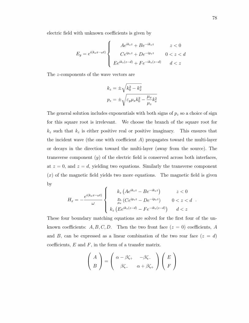
78
electric field with unknown coefficients is given by
Ey = ei(kxx−ωt)
Aeikzz +Be−ikzz
Ceipzz +De−ipzz
Eeikz(z−d) + Fe−ikz(z−d)
z < 0
0 < z < d
d < z
The z-components of the wave vectors are
kz = ±qk20 − k2x
pz = ±r
εyµxk20 −µxµzk2x
The general solution includes exponentials with both signs of pz so a choice of sign
for this square root is irrelevant. We choose the branch of the square root for
kz such that kz is either positive real or positive imaginary. This ensures that
the incident wave (the one with coefficient A) propagates toward the multi-layer
or decays in the direction toward the multi-layer (away from the source). The
transverse component (y) of the electric field is conserved across both interfaces,
at z = 0, and z = d, yielding two equations. Similarly the transverse component
(x) of the magnetic field yields two more equations. The magnetic field is given
by
Hx = −ei(kxx−ωt)
ω
kz¡Aeikzz −Be−ikzz¢
pzµx(Ceipzz −De−ipzz)
kz¡Eeikz(z−d) − Fe−ikz(z−d)¢
z < 0
0 < z < d
d < z
.
These four boundary matching equations are solved for the first four of the un-
known coefficients: A,B,C,D. Then the two front face (z = 0) coefficients, A
and B, can be expressed as a linear combination of the two rear face (z = d)
coefficients, E and F , in the form of a transfer matrix. A
B
=
α− βζ+ −βζ−βζ− α+ βζ+
E
F

79
where
α ≡ cos (pzd)β ≡ i sin (pzd)ζ± ≡ 1
2
µpzµxkz
± µxkzpz
¶We can then create a multi-layer structure by multiplying the transfer matrices of
the individual layers to form a combined transfer matrix. Each matrix transforms
the back surface coefficients to the front surface coefficients which, in turn, become
the back surface coefficients of the next layer.
M =M0M1...Mi...MN
We then impose our boundary condition and normalization. The incident wave
has unit magnitude, and there is no wave returning from infinity to the back face. 1
ρ
=M
τ
0
Solving, we find the reflection and transmission coefficient of the overall multi-layer
structure.
τ =1
M11
ρ =M21
M11
Since the transmitted wave coefficients are referred to the back face, the transmis-
sion coefficient is identical to the transfer function.
V.E Spatial Filters
We will use the following two basis matrices to represent all media used
for filter devices in this article.
σ0 =
1 0 0
0 1 0
0 0 1
σ1 =
1 0 0
0 1 0
0 0 −1

80
Figure V.2: Reflection and transmission coefficients versus incident angle for low,
high and band pass filters. For the high and low pass filters, the values for
θc ≡ sin−1 (kc/k0) are π/12, π/6, π/4, π/3 and 5π/12 going from dark to light
lines. The band pass filter has cutoffs, π/6 and π/3, with transmission shown
with a dark line and reflection shown with a light one. γ = 0.01 and k0d = 4π for
all filters except θc ≡ π/12 where k0d = 6π.
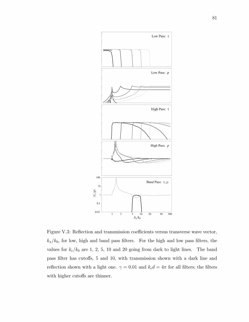
81
Figure V.3: Reflection and transmission coefficients versus transverse wave vector,
kx/k0, for low, high and band pass filters. For the high and low pass filters, the
values for kc/k0 are 1, 2, 5, 10 and 20 going from dark to light lines. The band
pass filter has cutoffs, 5 and 10, with transmission shown with a dark line and
reflection shown with a light one. γ = 0.01 and kcd = 4π for all filters; the filters
with higher cutoffs are thinner.

82
Figure V.4: Reflection and transmission of Gaussian beams incident on a band
pass filter. The band pass filter has θc = 24 and 58, kcd = 4π, and γ = 0.01.
The beams have width 10λ0 and incident angles 9, 34, and 69. The scale on the
transmission side is compressed to compensate for the attenuation of the beam.

83
Figure V.5: Low, high and band pass filtering of a square wave object. The square
wave has a fundamental period of λ0. The low pass filter has cutoff, kc/k0 = 5.
The band pass filter has cutoffs, kc/k0 = 5 and 20, and the high pass filter has
cutoff, kc/k0 = 20. γ = 0.01 and kcd = 4π for all three filters.

84
The first is just the identity matrix and the second is an indefinite matrix. Note
that they are both x-y isotropic. Though the solutions are computed above for
a specific orientation - where the plane of incidence is the x-z plane - the devices
discussed here will work equally well for a y-z plane of incidence, or any angle in
between.
Low pass filtering only requires isotropic media. We write the material
properties explicitly in terms of the cutoff, kc.
ε1 = µ1 =
µkck0+ iγ
¶σ0
ε2 = µ2 =
µ−kck0+ iγ
¶σ0
γ ¿ 1 is the parameter that introduces material loss. The cutoff, kc, determines
the upper limit of the pass band. This bilayer device has one layer of positive and
one layer of negative media. Note that ε = µ for both layers, so this device will be
polarization independent. We have included a small imaginary part, representing
material loss. Adjusting this loss parameter and the layer thickness controls the
filter roll off characteristics.
High pass filtering requires indefinite material property tensors.
ε1 = µ2 =kck0
σ1 + iγσ0
ε2 = µ1 = −kck0
σ1 + iγσ0
Here the cutoff, kc, determines the lower limit of the pass band. Note that ε ≈ −µfor both layers, so this device will not be polarization independent. Swapping
ε ↔ µ will effectively change the layer order. However, the layer order only
affects some subtle properties of the internal field and does not affect the overall
transmission or reflection properties, so this device will be externally polarization
independent.

85
Band pass filters are composed of four layers. A bilayer for the low pass
filtering and another bilayer for the high pass filtering. Since the second bilayer
reflects waves back into the first, one cannot rigorously compute the band pass
coefficients by multiplying two bilayer solutions together. A four layer transfer
matrix solution is required.
The transmission and reflection coefficient is shown for low, high and band
pass filters with various cutoffs in Figs. V.2 and V.3. Fig. V.2 shows filters with
cutoffs in the free space, propagating range, kc < k0. The independent variable is
given as an angle,
θ = sin−1kxk0,
since in this range the incident plane waves propagate in real directions. For
incident propagating waves, the reflection and transmission coefficients must, and
do obey
|ρ|2 + |τ |2 < 1
to conserve energy. Fig. V.3 shows filters with cutoffs in the free space, evanescent
range, kc > k0. The independent variable is given as, kx/k0. These filters can be
used to process near fields. In this range, transmission and reflection coefficients
need not be bound to values less than one since evanescent waves do not carry
energy. The upper kx roll off seen in the figure is undesirable for a high pass filter.
This roll off , discussed in detail elsewhere [41], is determined by the loss, γ, and
the thickness, d.
Fig. V.4 shows the field intensity pattern for several Gaussian beams
incident on a band pass filter with cutoffs in the propagating range. This multi-
layer structure transmits beams that are in a mid angle range and reflects beams
that are incident at small and large angles. This device is unusual in two ways.
Standard materials cannot reflect normally incident beams and transmit higher
angle ones. Also, though an upper critical angle is not unusual, it can only occur
when a beam is incident from a higher index media to a lower index media, and
not for a beam incident from free space, as it is in this case. The action of the

86
compensating layers also permits a greater transmittance with less distortion than
is possible with any single layer of normal materials. While it is possible to im-
plement an angular filter with a channeled, “mini-blinds” structure, such a device
could not be both translationally and rotationally invariant like the homogenous
implementation described here.
Fig. V.5 shows the effect of three different filters on an electromagnetic
spatial variation that has significant near field content. The spatial variation is
analogous to a diffraction grating back illuminated with a plane wave. The results
of low, high and band pass filtering are shown. The high pass filter shows the
edge detection properties of high pass filters. In this case, the edge information is
predominately in the near field components that would be lost in normal optical
components.
V.F Conclusion
We have shown how media with negative electromagnetic property ten-
sor elements can be used to construct high, low and band pass spatial filters with
cutoffs tunable both above and below the near/far field boundary. The far field
filters are particularly flexible and can be used either in transmission or reflec-
tion. We believe that these filters could find many uses in image processing and
communications applications.
V.G Acknowledgement
This chapter, in full, will be submitted for publication, with authors D.
Schurig and D. R. Smith.

87
Bibliography
[1] D. R. Smith et al., Phys. Rev. Lett. 84, 4184+ (2000).
[2] R. A. Shelby, D. R. Smith, and S. Schultz, Science 292, 79+ (2001).
[3] V. G. Veselago, Sov. Phys. Usp. 10, 509+ (1968).
[4] D. R. Smith and N. Kroll, Phys. Rev. Lett. 85, 3966+ (2000).
[5] P. M. Valanju, R. M. Walser, and A. P. Valanju, Phys. Rev. Lett. 88, 187401+(2002).
[6] J. B. Pendry, Phys. Rev. Lett. 85, 3966+ (2000).
[7] R. W. Ziolkowski and E. Heyman, Phys. Rev. E 6405, 056625+ (2001).
[8] M. Born and E. Wolf, in Principles of Optics (Cambridge University Press,Cambridge, UK, 1980), Chap. I.
[9] J. A. Kong, B. Wu, and Y. Zhang, Appl. Phys. Lett. 80, 2084+ (2002).
[10] M. Notomi, Phys. Rev. B 62, 10696+ (2000).
[11] B. Gralak, S. Enoch, and G. Tayeb, J. Opt. Soc. Am. A 17, 1012+ (2000).
[12] R. Ruppin, Physics Letters A 277, 61+ (2000).
[13] R. Ruppin, Journal of Physics: Condensed Matter 13, 1811+ (2001).
[14] P. Markos and C. M. Soukoulis, Physical Review E 65, 036622+ (2002).
[15] S. A. Tretyakov, Microwave and Optical Technology Letters 31, 163+ (2001).
[16] C. Caloz, C.-C. Chang, and T. Itoh, Journal of Applied Physics 90, 5483+(2001).
[17] E. Shamonina, V. A. Kalinin, K. H. Ringhofer, and L. Solymar, ElectronicsLetters 37, 1243+ (2001).
[18] Z. M. Zhang and C. J. Fu, Applied Physics Letters 80, 1097+ (2002).

88
[19] S. A. Ramakrishnan et al., J. Mod. Optics (2002).
[20] J. B. Pendry, A. J. Holden, D. Robbins, and W. J. Stewart, IEEE Transactionson Microwave Theory and Techniques 47, 2075+ (1999).
[21] J. B. Pendry, A. J. Holden, W. J. Stewart, and I. Youngs, Physical ReviewLetters 76, 4773+ (1996).
[22] D. R. Smith et al. (unpublished).
[23] S. John and T. Quang, Phys. Rev. Lett. 74, 3419+ (1995).
[24] A. F. Koenderink et al., Phys. Rev. Lett. 88, 143903/1 (2002).
[25] H. Kosaka et al., Phys. Rev. B 58, R10096 (1998).
[26] P. Halevi, A. A. Krokhin, and J. Arriaga, Phys. Rev. Lett. 82, 719+ (1999).
[27] L. D. Landau, E. M. Lifshitz, and L. P. Pitaevskii, in Electrodynamics ofContinuous Media (Pergamon Press, New York, 1984), Chap. X.
[28] J. A. Kong, Electromagnetic Wave Theory (Wiley-Interscience, New York,1990).
[29] I. V. Lindell, S. A. Tretyakov, K. I. Nikoskinen, and S. Ilvonen, Microwaveand Optical Technology Letters 31, 129+ (2001).
[30] These unusual classes of dispersion are not unknown in the context of electronsmoving in a periodic potential. When an electronic band structure has a saddlepoint the effective mass tensor is indefinite and analagous behavior is found.
[31] D. Sievenpiper et al., IEEE Transactions on Microwave Theory and Tech-niques 47, 2059+ (1999).
[32] K.-P. Ma, Y. Qian, and T. Itoh, IEEE Transactions on Microwave Theoryand Techniques 47, 1509+ (1999).
[33] D. Schurig et al. (unpublished).
[34] S. A. Ramakrishnan and J. B. Pendry (unpublished).
[35] D. R. Chowdhury, K. Bhattacharya, and A. Ghosh, Journal of Optics 29, 5+(2000).
[36] G. W. t’ Hooft, Physical Review Letters 87, 249701+ (2001).
[37] J. T. Shen and P. M. Platzman, Applied Physics Letters 80, 3286+ (2002).
[38] A. Lakhtakia, International Journal of Infrared and Millimeter Waves 23,339+ (2002).
[39] F. D. M. Haldane (unpublished).

89
[40] D. R. Smith and D. Schurig (unpublished).
[41] D. Schurig and D. R. Smith (unpublished).


![SOFT-FOCUSING IN ANISOTROPIC INDEFINITE MEDIA THROUGH ... In... · similar focusing to that seen in the negative index slab. Liu et al. [9] and Fang et al. [10] demonstrated this](https://static.fdocuments.in/doc/165x107/5eb549db9543f90e966a5ad7/soft-focusing-in-anisotropic-indefinite-media-through-in-similar-focusing.jpg)