PhD-Thesis

PhD Dissertation

International Doctorate School in Information andCommunication Technologies

DISI - University of Trento

QUERY ANSWERING OVER CONTEXTUALIZED

RDF/OWL KNOWLEDGE WITH EXPRESSIVE

BRIDGE RULES: DECIDABLE CLASSES

Mathew Joseph

Advisor: Dr. Luciano Serafini

Centre for Information Technology

Fondazione Bruno Kessler-IRST

April 2015

Defense Comittee

Prof. Alex BorgidaFaculty of Computer Science,Rutgers University, NJ, USA

Prof. Paolo BouquetDepartment of Information Science & Engineering (DISI),University of Trento, TN, Italy

Dr. Jerome EuzenatINRIA,Grenoble, Rhone Alpes, France

Prof. Enrico FranconiFaculty of Computer Science,Free University of Bozen-Bolzano, Italy

Abstract

In this thesis, we study the problem of reasoning and query answering over

contextualized knowledge in quad format augmented with expressive forall-

existential bridge rules. Such bridge rules contain conjunctions, existentially

quantified variables in the head, and are strictly more expressive than the bridge

rules considered so far in similar setting. A set of quads together with forall-

existential bridge rules is called a quad-system. We show that query answering

over quad-systems in their unrestricted form is undecidable, in general. We pro-

pose various subclasses of quad-systems, for which query answering is decid-

able. Context-acyclic quad-systems do not allow the context dependency graph

of the bridge rules to have cycles passing through triple-generating (value-

generating) contexts, and hence guarantees the chase (deductive closure) to

be finite. Csafe, msafe and safe classes of quad-systems restricts the structure

of descendance graph of Skolem blank nodes generated during chase process

to be directed acyclic graphs (DAGs) of bounded depth, and hence has finite

chases. RR and restricted RR quad-systems do not allow for the creation of

Skolem blank nodes, and hence restrict the chase to be of polynomial size.

Besides the undecidability result of unrestricted quad-systems, tight complex-

ity bounds has been established for each of the classes we have introduced.

We then compare the problems, (resp. classes,) we address (resp. derive) in

this thesis, for quad-systems with analogous problems (resp. classes) in the

realm of forall-existential rules. We show that the query answering problem

over quad-systems is polynomially equivalent to the query answering problem

over ternary forall-existential rules, and the technique of safety, we propose, is

strictly more expressive than existing well known techniques such joint acyclic-

ity and model maithful acyclicity, used for decidability guarantees, in the realm

of forall-existential rules.

Keywords[Contextualized RDF/OWL, Contextualized Knowledge Bases, Quads, QueryAnswering, Multi-Context Systems, Forall-Existential Rules, Datalog+-, De-scription Logics, Semantic Web, Knowledge Representation]

6

Acknowledgements

Firstly, I thank the almighty for extending all these gifts in this life. I express mygratitude to the members of the thesis defence committee, for the careful read-ing of the manuscript, for all the critics and comments that led me to improve thequality of this thesis. Also important is all the mentoring and personal advisesreceived from Prof. Gabriel Kuper over these years. Would like to remember allthe nostaligic memories spent with all the former and current members of theDKM, Shell group in FBK, namely Loris Bozzato, Francesco Corcoglionitti,Chiara Ghidini, Chiara di Francesco Marino, Marco Rospocher, Martin Ho-mola, Nahid Mahbub, Andrei Tamilin, Volha Bryl, Gaetano Calabrese, TahirKhan, Zolzaya Dashdorj, Giulio Petrucci, and Roberto Tiella (SE group). Alsomemories of the time spent at university of Bremen, where I did my internshipunder the guidance of Prof. Till Mossakowski, and time spent in close vicin-ity with Oliver Kutz, Christoph Lange in Spring 2012 was invaluable. Alsothe night bashes with my most lovable friends Matteo Aluigi, Gideon Njarko,Guido Sbrogio, Paolo Calanca, Aurora Sartori, Elisa Abetini, and Orlazzo Or-lazzi is unforgettable. Also, I gratefully acknowledge all of my friends fromindian community in Trento, Anil Kumar, Pradeep Warrier, Ajay tripathy, Man-ish Jain, Nainesh, Rupali Patel, Rohan, Deepa Fernandez, Soudip, Niyati RoyChowdhury, Tinku, Sajna Basheer, Swaytha Sasidharan, Lejo Joseph, Rahulwith whom we organized all the indian festivals, cooked and shared so manyrecipes. Also remember my friends Anna and Adam from Wroclaw, Christianand Lisa from Innsbruck who often visited me and made my days in Trento a“gem of my life”. Most and most importantly, I would like to thank my scien-tific guru, Luciano Serafini, for all the encouragement and scientific guidelines,for having been always open for discussions, personal advises, and for beingsuch a super cool advisor, over these years. Foremostly, I am deeply indepted

to my parents, especially my mother who passed away recently, whose over-whelming love, warmth, and advises have given me the strength to overcomethe thicks and thins of this life. I also acknowledge my sister and family for theimmense moral support in my downs.

8

Contents

1 Introduction 11.1 The Context . . . . . . . . . . . . . . . . . . . . . . . . . . . . 1

1.2 The Problem and Solution Overview . . . . . . . . . . . . . . . 1

1.2.1 Thesis Applications and Similar Problem Formulations . 8

1.2.2 Publications . . . . . . . . . . . . . . . . . . . . . . . . 14

1.3 Structure of the Thesis . . . . . . . . . . . . . . . . . . . . . . 15

2 Semantic Web Languages and Query Answering 172.1 Semantic Web Languages . . . . . . . . . . . . . . . . . . . . . 17

2.1.1 RDF Preliminaries . . . . . . . . . . . . . . . . . . . . 18

2.1.2 OWL Preliminaries . . . . . . . . . . . . . . . . . . . . 21

2.1.3 OWL 2 RL Profile . . . . . . . . . . . . . . . . . . . . 24

2.1.4 OWL 2 EL Profile . . . . . . . . . . . . . . . . . . . . 25

2.1.5 OWL-Horst Extension to RDF . . . . . . . . . . . . . . 26

2.1.6 Translations of OWL Statements to First Order LogicStatements . . . . . . . . . . . . . . . . . . . . . . . . 28

2.1.7 Forall-Existential (∀∃) Rules . . . . . . . . . . . . . . . 30

2.2 Query Answering over Ontologies . . . . . . . . . . . . . . . . 31

2.2.1 Chase of an Ontology . . . . . . . . . . . . . . . . . . . 33

2.2.2 Complexity Measures of Query Answering . . . . . . . 38

2.3 Computational Complexity Fundamentals . . . . . . . . . . . . 40

iii

3 Contextual Representation and Reasoning for Semantic Web: A Re-view on Existing Frameworks 453.1 Distributed Description Logics . . . . . . . . . . . . . . . . . . 46

3.2 E-connections . . . . . . . . . . . . . . . . . . . . . . . . . . . 49

3.3 Contextualized Knowledge Repository . . . . . . . . . . . . . . 54

3.4 Thesis Advancements . . . . . . . . . . . . . . . . . . . . . . . 58

3.4.1 Conjunctive Bridge Rules . . . . . . . . . . . . . . . . 58

3.4.2 Heterogeneous Bridge Rules . . . . . . . . . . . . . . . 59

3.4.3 Value Inventing Bridge Rules . . . . . . . . . . . . . . 60

3.4.4 Contextual Conjunctive Queries . . . . . . . . . . . . . 61

4 Query Answering over Quad-Systems and its Undecidability 634.1 Quad-Systems . . . . . . . . . . . . . . . . . . . . . . . . . . . 63

4.2 Query Answering on Quad-Systems . . . . . . . . . . . . . . . 67

4.2.1 Undecidability of Query Answering on Quad-Systems . 69

5 Context Acyclic Quad-Systems: Decidability via Acyclicity 735.1 Context Acyclic Quad-Systems: A Decidable Class . . . . . . . 77

5.2 Context Acyclic Quad-Systems: Computational Properties . . . 79

6 Csafe, Msafe, and Safe Quad-Systems: Restricting the DescendencyStructure of Skolem Blank-nodes 916.1 Csafe, Msafe, and Safe Quad-Systems: Decidable Classes . . . 96

6.2 Csafe, Msafe, and Safe Quad-Systems: Computational Properties 103

6.3 Procedure for Detecting Safe/Msafe/Csafe Quad-Systems . . . . 113

7 Range Restricted Quad-Systems 1217.1 Restricting to Range Restricted BRs . . . . . . . . . . . . . . . 121

7.2 Restricted RR Quad-Systems . . . . . . . . . . . . . . . . . . . 125

iv

8 Quad-Systems vs Forall-Existential rules 1278.1 Weak Acyclicity . . . . . . . . . . . . . . . . . . . . . . . . . . 1328.2 Joint Acyclicity . . . . . . . . . . . . . . . . . . . . . . . . . . 1368.3 Model Faithful Acyclicity (MFA) . . . . . . . . . . . . . . . . . 138

9 Related work 1419.1 Contexts and Distributed Logics . . . . . . . . . . . . . . . . . 1419.2 Temporal/Annotated RDF . . . . . . . . . . . . . . . . . . . . 1439.3 Description Logic Rules . . . . . . . . . . . . . . . . . . . . . 1449.4 ∀∃ rules, Tuple Generating Dependencies, Datalog+- rules . . . 1459.5 Data integration . . . . . . . . . . . . . . . . . . . . . . . . . . 1479.6 Distributed/Federated SPARQL Querying . . . . . . . . . . . . 148

10 Summary and Conclusion 149

Bibliography 153

A Appendix 167A.1 Appendix of Chapter 2 . . . . . . . . . . . . . . . . . . . . . . 167

A.1.1 RDF and RDFS Inference Rules . . . . . . . . . . . . . 167A.1.2 Ontology with only Infinite Models . . . . . . . . . . . 167

A.2 Appendix of Chapter 4 . . . . . . . . . . . . . . . . . . . . . . 169A.3 Appendix of Chapter 6 . . . . . . . . . . . . . . . . . . . . . . 175

v

List of Tables

1.1 Domain expansion inference rules of CKRRDF [75]. . . . . . . . 14

2.1 Semantics of OWL constructs . . . . . . . . . . . . . . . . . . 232.2 First order translation of DL concepts . . . . . . . . . . . . . . 292.3 First order translation of DL statements for DLs with simple roles 29

8.1 Edges induced in the dependency graph due to OWL-Horst in-ferencing . . . . . . . . . . . . . . . . . . . . . . . . . . . . . 135

10.1 Complexity info for various quad-system fragments . . . . . . . 150

A.1 RDF rules . . . . . . . . . . . . . . . . . . . . . . . . . . . . . 167A.2 RDFS rules . . . . . . . . . . . . . . . . . . . . . . . . . . . . 168

vii

List of Figures

1.1 Three different contexts resulting from three different viewpointson the same object . . . . . . . . . . . . . . . . . . . . . . . . 3

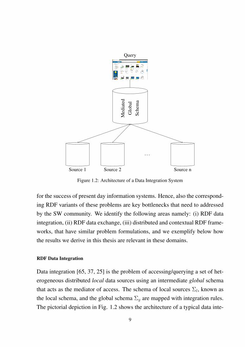
1.2 Architecture of a Data Integration System . . . . . . . . . . . . 9

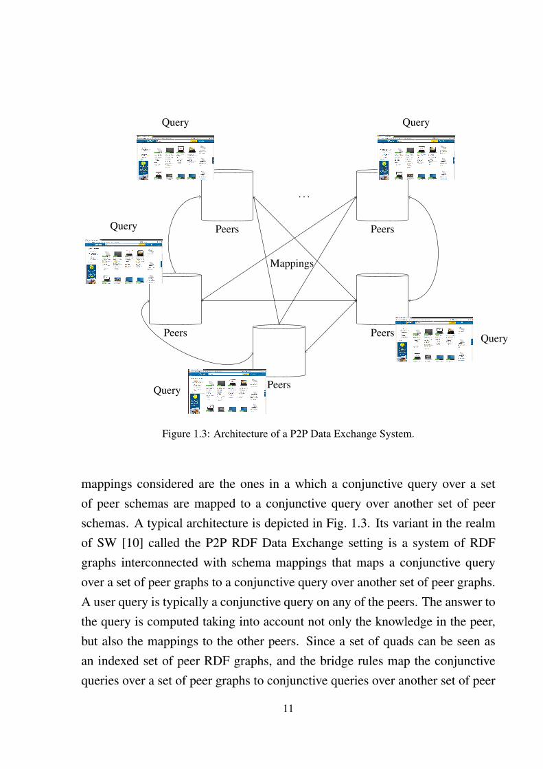
1.3 Architecture of a P2P Data Exchange System. . . . . . . . . . . 11

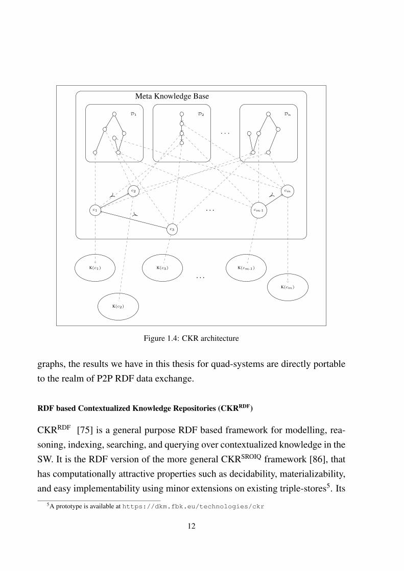
1.4 CKR architecture . . . . . . . . . . . . . . . . . . . . . . . . . 12

2.1 Visual rendering of a sample RDF graph . . . . . . . . . . . . . 19

2.2 Finite and infinite model of an EL ontology . . . . . . . . . . . 26

2.3 RDF graph translation of OWL ontology . . . . . . . . . . . . . 32

4.1 A CCQ over quad-system . . . . . . . . . . . . . . . . . . . . . 68

4.2 A sample CCQ: Intersecting objects in different contexts . . . . 68

5.1 Bridge rule: A mechanism for specifying propagation of knowl-edge between contexts. . . . . . . . . . . . . . . . . . . . . . . 77

5.2 Context dependency graph . . . . . . . . . . . . . . . . . . . . 78

5.3 Saturation of contexts . . . . . . . . . . . . . . . . . . . . . . . 80

6.1 Descendance graph of :b4 in Example 7. Note: n.d. labels arenot shown . . . . . . . . . . . . . . . . . . . . . . . . . . . . . 99

6.2 Descendance graph of Fig. 6.1 unraveled into a tree. Note: n.d.labels are not shown . . . . . . . . . . . . . . . . . . . . . . . . 105

8.1 Dependency graph of the quad-system in Example 7 of Chapter 6.136

ix

8.2 Context dependency graph of the quad-system in Example 7 ofChapter 6. . . . . . . . . . . . . . . . . . . . . . . . . . . . . . 136

10.1 Landscape of classes for quad-systems and ternary ∀∃ rules . . . 151

A.1 An infinite model . . . . . . . . . . . . . . . . . . . . . . . . . 168

x

Chapter 1

Introduction

1.1 The Context

In this thesis, we describe the challenges faced, techniques applied, and resultsobtained, in an attempt to extend the frontiers of query answering, representa-tion, and reasoning on contextually sensitive knowledge with particular focuson their applications in the realm of Semantic Web (SW) – the extension of theworld wide web that adds the power of logical reasoning leveraging knowledgerepresentation (KR) [18] languages with semantics such as resource descriptionframework (RDF) and web ontology language (OWL). With the proliferationof semantic knowledge on the web contributed from disparate users, pushingthe envelopes of contextual reasoning and query answering is the key to thegoal of successful realization of the SW. Keeping this goal in mind, duringthis endeavor we have applied techniques, tools and already developed theoriesfrom disciplines such as artificial intelligence, knowledge representation, anddatabases.

1.2 The Problem and Solution Overview

Businesses and organizations leveraging SW, its languages such as RDF andOWL, its interlinked constellation of ontologies, and exploiting semantic tech-

1

nologies to provide a richer set of services to their consumers are increasing,more than ever before. One of the main reasons for this widespread acceptanceof SW is its ‘open’ model. The model is called open as it seamlessly allowsanyone, anywhere in the world to freely publish knowledge artifacts, and allowweb portals/repositories to unrestrictedly open access points to their semanticdata. It is presumed that any knowledge contributor publish his/her perceptionabout a particular domain as an ontology in the SW, which is very much relativeto the contributor. Moreover, SW imposes no arbitration mechanism or stipu-lated qualifying criteria for the user provided content. Hence, the knowledgein the SW is referred to as ‘context-dependant’, as the truth value of any pieceof knowledge is often associated with an implicit context in which the piece ofknowledge is assumed to hold.

Example 1. Consider the triple (Bologna,rdf:type,Sausage) from theOntology available at link: http://athena.ics.forth.gr:9090/RDF/VRP/Examples/tap.rdf. Note that the truth value of this statement is rel-ative, and depends on the view point or socio-cultural background of its in-terpreter. Since for most people ‘Bologna’ is an Italian city, and for peoplewho hail from Italy or not aware of culinary jargons, the statement is absurd.Hence, unless one makes the context of the statement explicit, and is writtenas Cookery : (Bologna,rdf:type, Sausage) or UScuisine : (Bologna,rdf:type, Sausage).

As a result, a large number of initiatives have already been taken for extend-ing SW and its languages for the support for explication of contexts. One ofthe major outcomes of such initiatives is a knowledge format called quads thatextend the standard RDF triple with a fourth component which indicates thecontext in which the triple holds. A quad is a tuple c : (s, p, o), where (s, p, o)

is a standard RDF triple and c is the identifier of the context in which the tripleholds. As a result, more and more triple-stores are becoming quad-stores. Some

2

Front view (cfv)Side view (csv

)

Top view (ctv)cfv

csv

ctv

Figure 1.1: Three different contexts resulting from three different viewpoints on the same object

of the popular quad-stores are 4store1, Openlink Virtuoso 2, and some of the cur-rently popular triple-stores like Sesame3, Allegrograph4 internally keep track ofthe contexts of triples. Some of the recent initiatives in this direction have alsoextended existing formats like N-Triples to N-Quads [28], which the RDF 1.1has introduced as a W3C recommendation. The latest Billion triple challengedatasets have all been released in the N-Quads format. The following exampleexemplifies a situation in which quads can be handy to model multiple aspectsof the same world when viewed from different angles.

Example 2. Consider three knowledge creators viewing the same 3D object Afrom three different sides of the object as shown in Fig: 1.1. Since these per-sons are viewing the object from orthogonally different angles, their cognitiveperception of the object varies depending on the side from which the object isviewed. Suppose that the knowledge corresponding to these different percep-

1http://4store.org2http://virtuoso.openlinksw.com/rdf-quad-store/3http://www.openrdf.org/4http://www.franz.com/agraph/allegrograph/

3

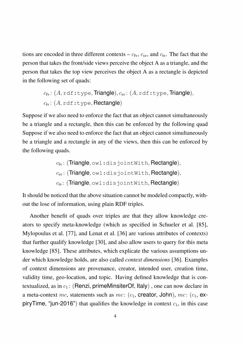
tions are encoded in three different contexts – cfv, csv, and ctv. The fact that theperson that takes the front/side views perceive the object A as a triangle, and theperson that takes the top view perceives the object A as a rectangle is depictedin the following set of quads:

cfv : (A,rdf:type,Triangle), csv : (A,rdf:type,Triangle),

ctv : (A,rdf:type,Rectangle)

Suppose if we also need to enforce the fact that an object cannot simultaneouslybe a triangle and a rectangle, then this can be enforced by the following quadSuppose if we also need to enforce the fact that an object cannot simultaneouslybe a triangle and a rectangle in any of the views, then this can be enforced bythe following quads.

cfv : (Triangle,owl:disjointWith,Rectangle),

csv : (Triangle,owl:disjointWith,Rectangle),

ctv : (Triangle,owl:disjointWith,Rectangle)

It should be noticed that the above situation cannot be modeled compactly, with-out the lose of information, using plain RDF triples.

Another benefit of quads over triples are that they allow knowledge cre-ators to specify meta-knowledge (which as specified in Schueler et al. [85],Mylopoulus et al. [77], and Lenat et al. [36] are various attributes of contexts)that further qualify knowledge [30], and also allow users to query for this metaknowledge [85]. These attributes, which explicate the various assumptions un-der which knowledge holds, are also called context dimensions [36]. Examplesof context dimensions are provenance, creator, intended user, creation time,validity time, geo-location, and topic. Having defined knowledge that is con-textualized, as in c1 : (Renzi, primeMinsiterOf, Italy) , one can now declare ina meta-context mc, statements such as mc : (c1, creator, John), mc : (c1, ex-piryTime, “jun-2016”) that qualifies the knowledge in context c1, in this case

4

its creator and expiry time. Another benefit of quads is the possibility of in-teresting ways for querying a contextualized knowledge base. For instance, ifcontext c1 contains knowledge about football world cup 2014 and context c2

about football euro cup 2012, then the query “who beat Italy in both world cup2014 and euro cup 2012” can be formalized as the conjunctive query:

c1: (x,beat, Italy) ∧ c2: (x,beat, Italy),

where x is a variable.From a reasoning point of view, since the contextual demarcation in a set

of quads allows for context-wise grouping and division of knowledge into de-coupled components that can simultaneously be fed to parallel reasoners, theapproach thus increases both scalability and efficiency enabling applications todo practical reasoning on the mammoth amount of knowledge in SW [17]. Be-sides the above flexibility, bridge rules [14] can be provided for inter-operatingthe knowledge in different contexts. Such rules are primarily of the form:

c : φ→ c′ : φ′ (1.1)

where φ, φ′ are both atomic concept (role) symbols, c, c′ are contexts. The se-mantics of such a rule is that if, for any ~a, φ(~a) holds in context c, then φ′(~a)

should hold in context c′, where~a is a unary/binary vector depending on whetherφ, φ′ are concept/role symbols.

Example 2 (Contd.). Going back to our 3D object example, suppose cactual bethe context that describes the object from an actual side-independent perspec-tive. Then the following fact “if an object is a triangle from both the front viewand the side view, then the object is actually a pyramid” can intuitively be spec-ified using the following bridge rule:

cfv : (x,rdf:type,Triangle) ∧ csv : (x,rdf:type,Triangle)→

cactual : (x,rdf:type,Pyramid)

5

Research Objectives of the Thesis Although bridge rules of the form (1.1) servethe purpose of specifying knowledge interoperability from a source context cto a target context c′, in many practical situations (a) there is the need of inter-operating multiple source contexts with multiple target contexts, for which thebridge rules of the form (1.1) are inadequate. Besides, (b) one would alsowant the ability of creating new values in target contexts for the bridge rules.Hence, more expressive bridge rules are required to address these aforemen-tioned issues. The main research focus of the thesis is the problem of (contex-tual) reasoning and query answering over contextualized RDF/OWL knowledge(generally, quads) in the presence of forall-existential bridge rules. We bringto the notice of the reader that although the contextual reasoning problem, tosome extent, has been touched by works such as Distributed Description Logics(DDL) [14], Klarman et al. [59], McCarthy et al. [74], and Distributed FirstOrder Logic (DFOL) [42] in the Description Logic (DL) [5] and first order logic(FOL) settings, the bridge rules we consider in this thesis are more expressive,with conjunctions and existential quantifiers in them, and satisfy requirements(a) and (b) mentioned above.

Overview of the Solution Approach From a computer science perspective, as withany problem, one of the first questions that we posed on a first rendezvous withour problem is that, “is the problem solvable at all?”. Meaning, can we devisealgorithms on a general purpose computer or a turing machine for solving theproblem. As we later show, query answering and reasoning over quad-systems(which are a set of quads plus forall-existential bridge rules) is undecidable.This means that there cannot exist an algorithm with soundness, completeness,and termination properties for the problem. Hence, one of the immediate ques-tions that arises is whether one can find large meaningful subclasses of the quad-systems for which the reasoning and query answering problem is decidable. Thebulk of this thesis describes and exemplifies such classes.

6

One of the first steps to be taken is to provide a semantics for interpretinga quad-system. The semantics should be broad enough to interpret arbitraryqueries from a commonly accepted query language, such as conjunctive queries.As we focus on the decision version of the problem, once a semantics is fixed,then the query answering problem is to decide for a given query, a vector offixed size, and a quad-system, whether the quad-system entails (w.r.t to thefixed semantics) the expression that results from substituting the vector on thevariables of the query. We now briefly glimpse through our solution approach.

We first formulate a basic semantics for interpreting and reasoning withknowledge in a quad-system. For this, we follow existing approaches such asDistributed Description Logics [14], CKR [86, 16], E-connections [64], andtwo-dimensional logic of contexts [59], to use a set of interpretation structuresas a model for contextualized knowledge. In this way, knowledge in each con-text is separately interpreted to a different interpretation structure. Also basedon the semantics provided, we derive procedures for conjunctive query answer-ing. For this, we formulate the notion of a distributed chase, which is an exten-sion of the standard chase [56, 1] that is widely used in the KR and DB settings,for similar purposes. The main contributions of this thesis work are:

1. We extend the standard RDF/OWL semantics to a context-based semanticsthat can be used for reasoning over contextualized RDF/OWL knowledge.Studying conjunctive query answering over quad-systems, we show thatthe entailment problem of conjunctive queries is undecidable for the mostgeneral class of quad-systems, called unrestricted quad-systems.

2. We define a class of quad-systems called context acyclic quad-systems, forwhich query answering is decidable and can be done by a forward chainingprocedure. The quad-systems in this class have the property that the de-pendency graph of the set of bridge rules do not have cycles going throughtriple generating contexts. We give both data and combined complexity of

7

conjunctive query entailment for the same.

3. We further extend the class of context acyclic to larger decidable classescalled csafe, msafe, and safe quad-systems, for which we give both dataand combined complexities of conjunctive query entailment. These classesare based on the constrained DAG structure of Skolem blank nodes gener-ated during the chase construction. We also provide decision proceduresto decide whether an input quad-system is safe (csafe, msafe) or not. Alsoin this case, a forward chaining procedure based on the restricted versionof standard chase is provided for checking entailment of queries.

4. Subsequently, we derive less expressive classes, RR and restricted RRquad-systems, for which no Skolem blank nodes are generated during thechase construction. This class is characterized by the property that anyquad-system in this class does not contain existentially quantified variablesin their bridge rules.

5. We also show that the class of unrestricted quad-systems is equivalent tothe class of ternary ∀∃ rule sets, which are the class of ∀∃ rule sets whosepredicates have arity less than or equal to three. We compare the derivedclasses of quad-systems with well known subclasses of ∀∃ rule sets, suchas weakly acylic, jointly acyclic and model faithful acyclic rule sets. Animportant result is that the technique of safety that we propose subsumesthese other techniques, in expressivity, and hence, can be used in the ∀∃settings to derive expressive recognizable classes.

1.2.1 Thesis Applications and Similar Problem Formulations

At the time when the computer science discipline is challenged with the prob-lem of managing the massive and continuous data generation rates, techniquesfor accessing, integrating, exchanging, and inferencing over this data is the key

8

Source 1 Source 2

. . .

Source n

Med

iate

dG

loba

lSc

hem

a

Query

Figure 1.2: Architecture of a Data Integration System

for the success of present day information systems. Hence, also the correspond-ing RDF variants of these problems are key bottlenecks that need to addressedby the SW community. We identify the following areas namely: (i) RDF dataintegration, (ii) RDF data exchange, (iii) distributed and contextual RDF frame-works, that have similar problem formulations, and we exemplify below howthe results we derive in this thesis are relevant in these domains.

RDF Data Integration

Data integration [65, 37, 25] is the problem of accessing/querying a set of het-erogeneous distributed local data sources using an intermediate global schemathat acts as the mediator of access. The schema of local sources Σl, known asthe local schema, and the global schema Σg are mapped with integration rules.The pictorial depiction in Fig. 1.2 shows the architecture of a typical data inte-

9

gration scenario. In the traditional version of the problem, both Σl and Σg aresets of relation symbols. A typical solution approach is to translate queries overΣg to queries over Σl that can be evaluated on the local sources. Yet another so-lution approach is to materialize the global schema so that queries can directlybe executed on it.

Off late the variant of the problem pertaining to the Semantic Web casehas drawn significant attention [26]. In this case, Σl is an (indexed) set ofRDF/OWL graphs, whose members represent the local sources and Σg is anindexed set of RDF/OWL graphs, whose members represent the global datasources. Furthermore, the typical architecture of the data integration can be ofone of the following three types: (i) Global as view (GAV) architecture, (ii) Lo-cal as view (LAV) architecture, and GLAV (Global and Local as view) architec-ture. In the GAV type, each global RDF graph is mapped on to a (conjunctive)query over the set of local RDF graphs. Whereas in the LAV variant, each localRDF graph is mapped on to a (conjunctive) query over the set of global RDFgraphs. In a GLAV setting, which is a generalization of both GAV and LAV,(conjunctive) queries over the set of local graphs are mapped on to (conjunc-tive) queries over the set of global RDF graphs. As a set of quads Q can be seenas an indexed set of RDF graphs indexed by the context identifiers in Q, thecorrespondence between quad-systems and GLAV RDF data integration lies inthe fact that both the integration rules and bridge rules are implications from aset of quad-patterns (called the body) to a another set of quad-patterns (calledthe head). Hence, we deem the outcomes of this thesis to be straightforwardlypropagatable to the problem of RDF data integration.

Peer-to-Peer RDF Data Exchange

The classical peer-to-peer (P2P) data exchange setting [40, 2] is a system ofrelational databases (called peers) interconnected using schema mappings thatspecify various dependency relations between the peer schemas. Typical schema

10

Peers

Peers

Peers

. . .

PeersPeers

QueryQuery

Query

Query

Query

Mappings

Figure 1.3: Architecture of a P2P Data Exchange System.

mappings considered are the ones in a which a conjunctive query over a setof peer schemas are mapped to a conjunctive query over another set of peerschemas. A typical architecture is depicted in Fig. 1.3. Its variant in the realmof SW [10] called the P2P RDF Data Exchange setting is a system of RDFgraphs interconnected with schema mappings that maps a conjunctive queryover a set of peer graphs to a conjunctive query over another set of peer graphs.A user query is typically a conjunctive query on any of the peers. The answer tothe query is computed taking into account not only the knowledge in the peer,but also the mappings to the other peers. Since a set of quads can be seen asan indexed set of peer RDF graphs, and the bridge rules map the conjunctivequeries over a set of peer graphs to conjunctive queries over another set of peer

11

Meta Knowledge Base

D1 D2

. . .

Dn

c1

c2

c3

. . . cm-1

cm

≺

�

≺

K(c1)

K(c2)

K(c3)

. . .K(cm-1)

K(cm)

Figure 1.4: CKR architecture

graphs, the results we have in this thesis for quad-systems are directly portableto the realm of P2P RDF data exchange.

RDF based Contextualized Knowledge Repositories (CKRRDF)

CKRRDF [75] is a general purpose RDF based framework for modelling, rea-soning, indexing, searching, and querying over contextualized knowledge in theSW. It is the RDF version of the more general CKRSROIQ framework [86], thathas computationally attractive properties such as decidability, materializability,and easy implementability using minor extensions on existing triple-stores5. Its

5A prototype is available at https://dkm.fbk.eu/technologies/ckr

12

main facet is the organization of contexts into hierarchies that allows to makeadditional inferences in individual contexts. This is quite intuitive as contextsrepresent real world domains, and real world domains can naturally be orderedinto hierarchies. Hence, the language of CKR contains a cover relation ≺ oncontexts, that is a strict partial order. In addition, contexts are also associatedwith context dimensions {Di = 〈Di,≺i〉}i=1...n, each of which is a strict poset,with a strict partial order ≺i over the set of values Di. Example of context di-mensions are time, topic, geolocations etc. The architecture of the CKRRDF isgiven in Fig. 1.4. Any knowledge statement should be defined w.r.t to a con-text, and hence belong to a context. Hence, in CKRRDF, the most atomic pieceof knowledge statement is a quad.

The main component of the CKR is the meta knowledge base cmk, which it-self is a context. It contains various definitions that relate other contexts to theirdimension values, statements about various dimensions Di, and the propertiesof their cover relation≺i. The strict partial order property of≺i can be imposedby the following bridge rules:

cmk : (x1,≺i, z1) ∧ cmk : (z1,≺i, x2)→ cmk : (x1,≺i, x2)

cmk : (x1,≺i, x1)→

where the latter BR is a a negative constraint that states the negation of its body.The above BRs are instantiated for ≺i, for i = 1 . . . n. Also the cover relationof contexts, ≺, is defined on top of the cover relation ≺i of the dimensions.

n∧i=1

[cmk : (c,Di, vi) ∧ cmk : (c′,Di, v′i) ∧ cmk : (vi,≺i, v′i)]→ cmk : (c,≺, c′)

cmk : (x1,≺, z1) ∧ cmk : (z1,≺, x2)→ cmk : (x1,≺, x2)

cmk : (x1,≺, x1)→

Note that the second and third of the above set of rules impose the strict partialorder on the context cover relation ≺. Each triple (s, p, o) in the object knowl-edge K(c) of context c is defined as a quad c : (s, p, o). Table 1.1 encodes the

13

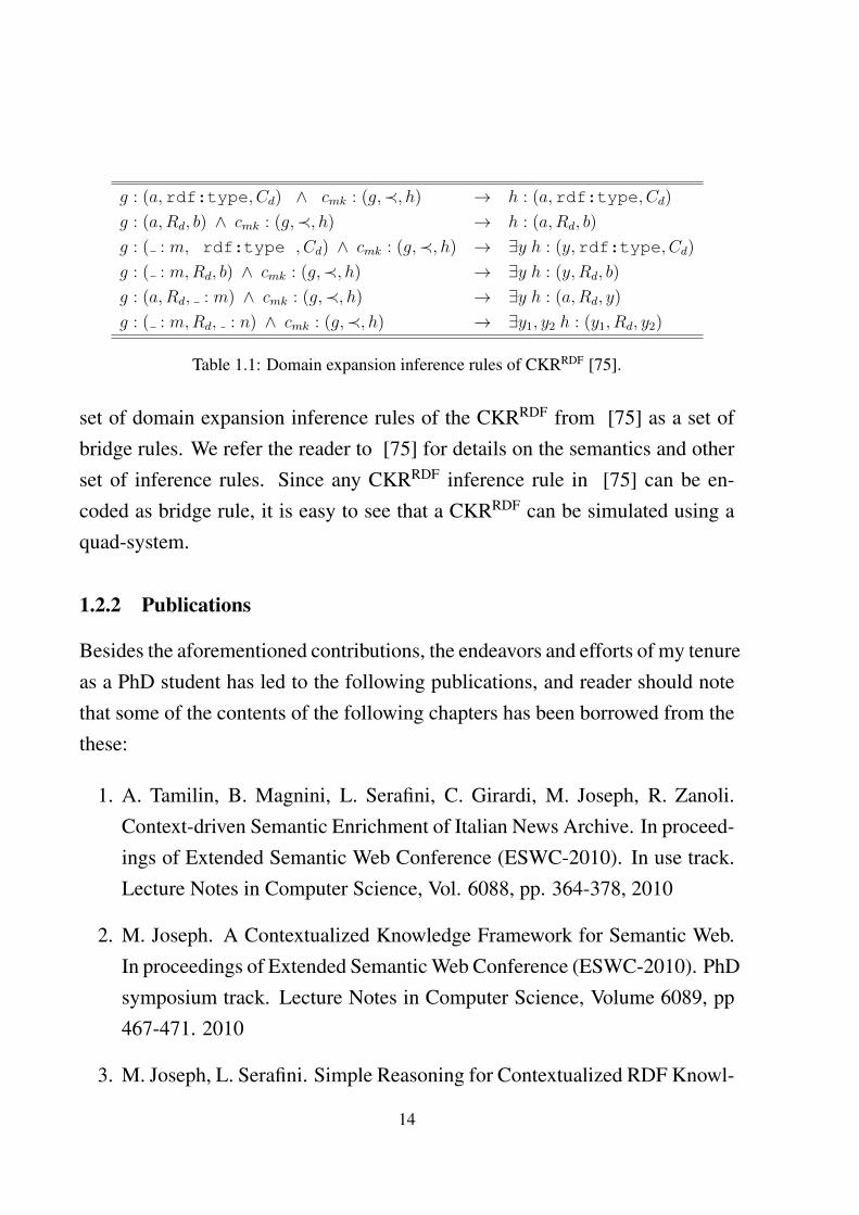
g : (a,rdf:type, Cd) ∧ cmk : (g,≺, h) → h : (a,rdf:type, Cd)

g : (a,Rd, b) ∧ cmk : (g,≺, h) → h : (a,Rd, b)

g : ( : m, rdf:type , Cd) ∧ cmk : (g,≺, h) → ∃y h : (y,rdf:type, Cd)

g : ( : m,Rd, b) ∧ cmk : (g,≺, h) → ∃y h : (y,Rd, b)

g : (a,Rd, : m) ∧ cmk : (g,≺, h) → ∃y h : (a,Rd, y)

g : ( : m,Rd, : n) ∧ cmk : (g,≺, h) → ∃y1, y2 h : (y1, Rd, y2)

Table 1.1: Domain expansion inference rules of CKRRDF [75].

set of domain expansion inference rules of the CKRRDF from [75] as a set ofbridge rules. We refer the reader to [75] for details on the semantics and otherset of inference rules. Since any CKRRDF inference rule in [75] can be en-coded as bridge rule, it is easy to see that a CKRRDF can be simulated using aquad-system.

1.2.2 Publications

Besides the aforementioned contributions, the endeavors and efforts of my tenureas a PhD student has led to the following publications, and reader should notethat some of the contents of the following chapters has been borrowed from thethese:

1. A. Tamilin, B. Magnini, L. Serafini, C. Girardi, M. Joseph, R. Zanoli.Context-driven Semantic Enrichment of Italian News Archive. In proceed-ings of Extended Semantic Web Conference (ESWC-2010). In use track.Lecture Notes in Computer Science, Vol. 6088, pp. 364-378, 2010

2. M. Joseph. A Contextualized Knowledge Framework for Semantic Web.In proceedings of Extended Semantic Web Conference (ESWC-2010). PhDsymposium track. Lecture Notes in Computer Science, Volume 6089, pp467-471. 2010

3. M. Joseph, L. Serafini. Simple Reasoning for Contextualized RDF Knowl-

14

edge. In Proceedings of Workshop on Modular Ontologies (WOMO-2011),Volume 230, IOS Press, Frontiers in Artificial Intelligence and Applica-tions. PP. 79-93. 2011

4. M. Joseph, G. Kuper, L. Serafini. Query Answering over ContextualizedRDF Knowledge with Forall-Existential Bridge Rules: Attaining Decid-ability using Acyclicity. In Proceedings of Italian Conference in Compu-tational Logic (CILC-2014). Volume 1195 of CEUR Workshop Proceed-ings, pages 210-224, CEUR-WS.org, 2014

5. M. Joseph, G. Kuper, L. Serafini. Query Answering over ContextualizedRDF/OWL Knowledge with Forall-Existential Bridge Rules: AttainingDecidability using Acyclicity. In Proceedings of International Conferencein Web Reasoning and Rule Systems (RR-2014). Springer Lecture Notesin Computer Science Volume 8741 pp. 60-75, 2014

6. M. Joseph, G. Kuper, T. Mossakowski, L. Serafini. Query Answeringover Contextualized RDF/OWL Knowledge with Forall-Existential BridgeRules: Decidable Finite Extension Classes. Semantic Web Journal (IOSPress). To Appear. 2015.

1.3 Structure of the Thesis

The thesis is structured as follows. In Chapter 2, we give a review of the state-of-the-art ontology languages relevant for the SW, glimpsing through languagessuch as RDF, OWL, and forall-existential rule fragment of first order logic. Wealso give an account on query answering over these languages, touching notionssuch as chase and its variants, and brief through the computational complexityfundamentals relevant for this thesis. In Chapter 3, we give a review on theexisting frameworks for contextual knowledge modelling relevant to the SW,

15

and then give an account on the shortcomings of these frameworks that moti-vates this thesis work and its contributions. In Chapter 4, we formally describethe main problem dealt by this thesis – The problem of query answering overcontextualized RDF knowledge with forall-existential bridge rules and its unde-cidability, introducing notions such as quad-graphs, bridge rules, quad-systems,and the problem of query answering on quad-systems and its undecidability.In Chapter 5, we describe a subclass of quad-systems for which the query an-swering problem is decidable. The class, which we call context acyclic quad-systems, ensures decidability by not allowing cyclic paths that involve blanknode generating contexts (TGCs) in the context dependency graph. Furtherin Chapter 6, we give more expressive classes of quad-systems namely csafe,msafe, and safe classes that strictly subsume the cacyclic quad-systems, basedon bounded depth DAG structure of Skolem blank nodes generated in the chase.For tractability reasoning, we subsequently in Chapter 7, derive less expressiveRR and restricted RR quad-systems, for which data complexity of query an-swering is tractable. Both these classes do not allow the generation of Skolemblank nodes in their chases. In Chapter 8, we compare the classes we derivedwith well known decidable classes in the realm of forall-existential rules. InChapter 9, we detail the related work relevant for this thesis and summarize theresults obtained in Chapter 10.

16

Chapter 2

Semantic Web Languages and QueryAnswering

In this chapter, we give an overview of SW concepts relevant to this thesis, in-troducing certain well known notations and parlances already existing in theliterature. We review some of the ubiquitous languages used for representingknowledge in the context of SW. We also discuss briefly the topic query answer-ing over knowledge defined using these languages. A few well known complex-ity classes relevant to the discussion in this thesis are concisely glimpsed.

2.1 Semantic Web Languages

SW languages are KR languages with particular emphasis on the representationand reasoning of knowledge and resources on the (world wide) web. Apart frombeing a formal logical language with semantics, the ideosyncratic feature ofsuch a language is the use of uniform resource identifiers (URI) for the constantsin the language. A URI specifies a resource by name in a particular namespace,and can be used to identify a resource without implying its location or how toaccess it. A URI can denote anything such as a person, place, or, in general,a logical or physical object in the universe or web. Though proposals exist forencoding uniquely identifying information of resources represented by URIs in

17

their syntax, currently available web standards are not adequate for this.

2.1.1 RDF Preliminaries

Let U be the set of uniform resource identifiers (URIs), B the set of blanknodes1, and L the set of literals. The set C = U ∪ B ∪ L are called the set of(RDF) constants. Any (s, p, o) ∈ C×C×C is called a generalized RDF triple(from now on, just triple). A generalized RDF graph (from now on, just graph)is defined as a set of triples. For any graph g, U(g),B(g),L(g), C(g) denoterespectively, the set of URIs, blank nodes, literals, constants in g. Some of thecommonly known syntaxes for serializing graphs are RDF/XML, RDF/JSON,N-Triples, Turtle, etc.

Example 1. The following is an example of a graph in Turtle syntax. The graphencodes information such as – the URI geonames:germany is related to the URIgeonames:argentina by the property :defeats, and also the former and latter areobjects of classes dbpedia:Champion and dbpedia:RunnerUp, respectively, bothof which in turn are objects of the meta class rdfs:Class.

@prefix rdf: <http://www.w3.org/1999/02/22-rdf-syntax-ns#>.

@prefix rdfs: <http://www.w3.org/2000/01/rdf-schema#>.

@prefix dbpedia: <http://dbpedia.org/resource#>.

@prefix geonames: <http://geonames.org/ontology#>.

@base: <http://mynamespace.org/ontology#>.

geonames:germany rdf:type dbpedia:Champion ;

:defeats geonames:argentina .

geonames:argentina rdf:type dbpedia:RunnerUp.

dbpedia:Champion rdf:type rdfs:Class.

dbpedia:RunnerUP rdf:type rdfs:Class.

1a.k.a labelled nulls

18

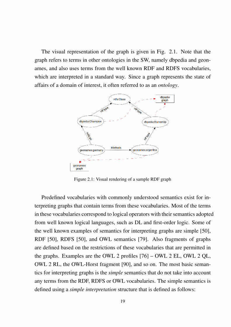
The visual representation of the graph is given in Fig. 2.1. Note that thegraph refers to terms in other ontologies in the SW, namely dbpedia and geon-ames, and also uses terms from the well known RDF and RDFS vocabularies,which are interpreted in a standard way. Since a graph represents the state ofaffairs of a domain of interest, it often referred to as an ontology.

Figure 2.1: Visual rendering of a sample RDF graph

Predefined vocabularies with commonly understood semantics exist for in-terpreting graphs that contain terms from these vocabularies. Most of the termsin these vocabularies correspond to logical operators with their semantics adoptedfrom well known logical languages, such as DL and first-order logic. Some ofthe well known examples of semantics for interpreting graphs are simple [50],RDF [50], RDFS [50], and OWL semantics [79]. Also fragments of graphsare defined based on the restrictions of these vocabularies that are permitted inthe graphs. Examples are the OWL 2 profiles [76] – OWL 2 EL, OWL 2 QL,OWL 2 RL, the OWL-Horst fragment [90], and so on. The most basic seman-tics for interpreting graphs is the simple semantics that do not take into accountany terms from the RDF, RDFS or OWL vocabularies. The simple semantics isdefined using a simple interpretation structure that is defined as follows:

19

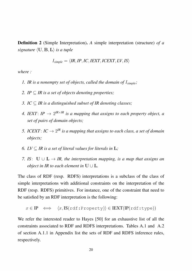
Definition 2 (Simple Interpretation). A simple interpretation (structure) of a

signature 〈U,B,L〉 is a tuple

Isimple = 〈IR, IP, IC, IEXT, ICEXT,LV, IS〉

where :

1. IR is a nonempty set of objects, called the domain of Isimple;

2. IP ⊆ IR is a set of objects denoting properties;

3. IC ⊆ IR is a distinguished subset of IR denoting classes;

4. IEXT : IP → 2IR×IR is a mapping that assigns to each property object, a

set of pairs of domain objects;

5. ICEXT : IC→ 2IR is a mapping that assigns to each class, a set of domain

objects;

6. LV ⊆ IR is a set of literal values for literals in L;

7. IS : U ∪ L → IR, the interpretation mapping, is a map that assigns an

object in IR to each element in U ∪ L.

The class of RDF (resp. RDFS) interpretations is a subclass of the class ofsimple interpretations with additional constraints on the interpretation of theRDF (resp. RDFS) primitives. For instance, one of the constraint that need tobe satisfied by an RDF interpretation is the following:

x ∈ IP ⇐⇒ 〈x, IS(rdf:Property)〉 ∈ IEXT(IP(rdf:type))

We refer the interested reader to Hayes [50] for an exhaustive list of all theconstraints associated to RDF and RDFS interpretations. Tables A.1 and A.2of section A.1.1 in Appendix list the sets of RDF and RDFS inference rules,respectively.

20

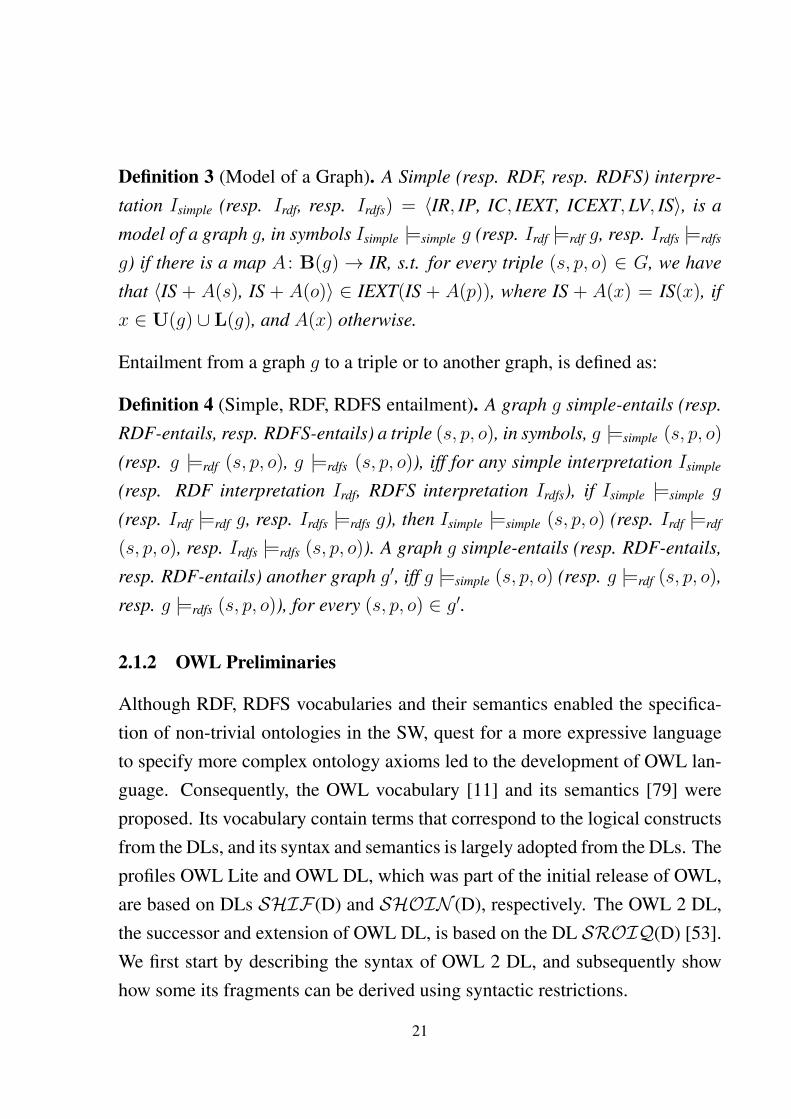
Definition 3 (Model of a Graph). A Simple (resp. RDF, resp. RDFS) interpre-

tation Isimple (resp. Irdf, resp. Irdfs) = 〈IR, IP, IC, IEXT, ICEXT,LV, IS〉, is a

model of a graph g, in symbols Isimple |=simple g (resp. Irdf |=rdf g, resp. Irdfs |=rdfs

g) if there is a map A : B(g)→ IR, s.t. for every triple (s, p, o) ∈ G, we have

that 〈IS + A(s), IS + A(o)〉 ∈ IEXT(IS + A(p)), where IS + A(x) = IS(x), if

x ∈ U(g) ∪ L(g), and A(x) otherwise.

Entailment from a graph g to a triple or to another graph, is defined as:

Definition 4 (Simple, RDF, RDFS entailment). A graph g simple-entails (resp.

RDF-entails, resp. RDFS-entails) a triple (s, p, o), in symbols, g |=simple (s, p, o)

(resp. g |=rdf (s, p, o), g |=rdfs (s, p, o)), iff for any simple interpretation Isimple

(resp. RDF interpretation Irdf, RDFS interpretation Irdfs), if Isimple |=simple g

(resp. Irdf |=rdf g, resp. Irdfs |=rdfs g), then Isimple |=simple (s, p, o) (resp. Irdf |=rdf

(s, p, o), resp. Irdfs |=rdfs (s, p, o)). A graph g simple-entails (resp. RDF-entails,

resp. RDF-entails) another graph g′, iff g |=simple (s, p, o) (resp. g |=rdf (s, p, o),

resp. g |=rdfs (s, p, o)), for every (s, p, o) ∈ g′.

2.1.2 OWL Preliminaries

Although RDF, RDFS vocabularies and their semantics enabled the specifica-tion of non-trivial ontologies in the SW, quest for a more expressive languageto specify more complex ontology axioms led to the development of OWL lan-guage. Consequently, the OWL vocabulary [11] and its semantics [79] wereproposed. Its vocabulary contain terms that correspond to the logical constructsfrom the DLs, and its syntax and semantics is largely adopted from the DLs. Theprofiles OWL Lite and OWL DL, which was part of the initial release of OWL,are based on DLs SHIF(D) and SHOIN (D), respectively. The OWL 2 DL,the successor and extension of OWL DL, is based on the DL SROIQ(D) [53].We first start by describing the syntax of OWL 2 DL, and subsequently showhow some its fragments can be derived using syntactic restrictions.

21

An OWL signature is given by the 4-tuple 〈ΣC , ΣP , ΣI , ΣL〉, where ΣC is aset of atomic concepts, ΣP is a set of atomic roles, ΣI , a set of individuals, andΣL, the set of literals. An OWL Concept C over an OWL signature Sig = 〈ΣC ,ΣP , ΣI , ΣL〉, is inductively defined as:

C := A | C u C | C t C | ¬C | ∃R.C | ∀R.C |

≥ nR.C | ≤ nR.C | ∃R.Self | {a1, a2, ..., am} | > | ⊥

where A ∈ ΣC , R is an OWL Role (see below) over signature Sig, a1, ..., am ∈ΣI , n is a natural number, > the top concept represents all the objects in thedomain, and ⊥ the bottom concept has no individuals. An OWL Role R overthe signature Sig is defined as:

R := P | R− | R ◦R ◦ ... ◦R | U

where P ∈ ΣP , U is the universal role and is equivalent to > × >. An OWLOntology O = 〈T ,R,A〉 over an OWL signature Sig, where T is a set ofstatements of the form C v D, where C,D are OWL Concepts over Sig, R isa set of statements of the form R v S or Disjoint(R, S) , where R, S are OWLRoles over Sig. Note that constructs such as Transitive(R), Symmetric(R),Reflexive(R), Irreflexive(R), Funtional(R) can be expressed as R◦R v R, R−

v R,> v ∃R.Self,∃R.Self v ⊥,> v≤ 1.R, respectively. OWL 2 DL [51]has further restrictions over concept, role constructors and assertions. It requiresthe role hierarchies to be regular, i.e. it does not permit cyclic hierarchies of theform R v R1, R1 v R2, . . . , Rn v R, and further constrains roles in cardinalityrestrictions to be simple2. A is a set of statements of the form:

C(a) | R(a, b)|¬P (a, b) | a = b | a 6= b

where C is an OWL Concept over Sig, P ∈ ΣP , R an OWL role over Sig, a isan individual over Sig, b an indivual or a literal over Sig.

2Simple roles are roles that are not implied by composition of other roles

22

Construct type Syntax SemanticsA ∈ ΣC AI ⊆ ∆I

> ∆I

⊥ ∅¬C ∆I \ CI

∃R.C {x|(x, y) ∈ RI&y ∈ CI}∀R.C {x|(x, y) ∈ RI implies y ∈ CI}

Concept ≥ nR.C {x|#{y|(x, y) ∈ RI&y ∈ CI} ≥ n}≤ nR.C {x|#{y|(x, y) ∈ RI&y ∈ CI} ≤ n}{a} {aI}

C uD CI ∩DI

C tD CI ∪DI

∃R.Self {x|(x, x) ∈ RI}P ∈ ΣP P I ⊆ ∆I ×∆I

R− {(y, x)|(x, y) ∈ RI}Role U ∆I ×∆I

¬R ∆I ×∆I \ RI

R ◦ S RI ◦ SI

Individual a ∈ ΣI aI ∈ ∆I

Plain Literal l ∈ ΣL lI = l ∈ ∆I

C v D CI ⊆ DI

R v S RI ⊆ SI

Assertions C(a) aI ∈ CI

R(a, b) (aI , bI ) ∈ RI

a = b aI = bI

a 6= b aI 6= bI

Table 2.1: Semantics of OWL constructs

Definition 5 (OWL Interpretation). An OWL Interpretation w.r.t. a signature

〈ΣC , ΣP , ΣI , ΣL〉 is a structure Iowl = (∆I , .I) where ∆I , called the domain of

Iowl. and .I is the valuation function s.t., for each A ∈ ΣC , AI ⊆ ∆I , for each

P ∈ ΣP , PI ⊆ ∆I ×∆I , for each a ∈ ΣI , a

I ∈ ∆I and for each l ∈ ΣL, lI =

l ∈ ∆I .

Definition 6 (Model of an OWL Ontology). An OWL Interpretation Iowl =

(∆I , .I) w.r.t. a signature 〈ΣC , ΣP , ΣI , ΣL〉 is said to be a model of an OWL

ontology O = 〈T ,R,A〉, in symbols Iowl |=owl O iff Iowl |=owl St, for every

assertion St ∈ T ∪R ∪A as per conditions in Table 2.1.

Definition 7 (OWL entailment). An OWL OntologyO, OWL-entails a statement

St, in symbols O |=owl St iff for any OWL model Iowl, if Iowl |=owl O, then

Iowl |=owl St. An OWL ontology O OWL-entails another OWL ontology O′, iff

O |=owl st, for any st ∈ O′.

Thanks to the popularity of the OWL language, a large number of graphs pub-lished in the SW extensively contain OWL vocabularies. But due to the high

23

computational complexity of reasoning with expressive OWL ontologies, webscale reasoning became impractical. The complexity of checking concept sat-isfaction with OWL 2 DL is 2NEXPTIME-hard, and no practical, sound, andcomplete algorithm is known yet for conjunctive query answering over OWLDL and OWL 2 DL. Consequently, less expressive profiles of OWL languagewas derived.

2.1.3 OWL 2 RL Profile

OWL 2 RL profile [76] is a part of the OWL 2 [51] standard that enables the useof a substantial part of the OWL vocabulary in an ontology, yet allows efficientreasoning and query answering. For simplicity, we exclude concrete-domains,data properties, and key assertions. Given the set of concept names ΣC , rolenames ΣP , and individual names ΣI , OWL 2 RL concepts are defined by thefollowing productions:

lc := A | {a} | lc u lc | lc t lc | ∃R.lc | ∃R.>

rc := A | ¬lc | rc u rc | ∀R.rc | ∃R.{a} | ≤ nR.lc | ≤ nR.>

mc := A | ∃P.{a} |mc umc

where A ∈ ΣC , a ∈ ΣI , R is an OWL 2 RL role (see below), and n = 0, 1.OWL 2 RL concept axioms are of the form:

LC v RC

where LC := lc | mc and RC := rc | mc. OWL 2 RL roles are given by theproduction

R := P | P−

where P ∈ ΣP . OWL 2 RL property axioms are of one of the following forms:

24

R v R | domain(R, rc) | range(R, rc) | disjoint(R,R)

| functional(R) | inversefunctional(R) | symmetric(R)

| asymmetric(R) | transitive(R) | irreflexive(R)

OWL 2 RL individual axioms are of the form C(a) or R(a, b) where a, b ∈ ΣI ,C is a OWL 2 RL concept of the form rc, R is an OWL 2 RL property. AnOWL 2 RL ontology O is a triple 〈T ,R,A〉 where T is a set of OWL 2RL concept axioms, R is a set of OWL 2 RL property axioms, A is a setof OWL 2 RL individual axioms. An OWL 2 RL graph is an OWL 2 RLontology translated to an RDF graph using the standard translation definedin OWL 2 Mapping to RDF graphs [80]. OWL 2 RL RDF rules [76] is apartial axiomatization of OWL 2 RL. These set of rules provides axiomati-zations for OWL constructs like owl:intersectionOf, owl:unionOf,owl:complementOf which are not provided by OWL-Horst. Although de-ductive closure w.r.t. these rules for any graph g can be computed in PTIME,Kroetzsch [61] showed that the set of rules are incomplete for the OWL 2 RLfragment of OWL for reasoning tasks such as computing subsumptions, whichis co-NP Hard.

2.1.4 OWL 2 EL Profile

The EL fragment of OWL 2 is intended for applications that demand a fairamount of terminological expressivity, yet require tractable reasoning servicesfor subsumption checking and instance checking. The description logic EL [4]is the foundation of OWL 2 EL fragment. For simplicity, we exclude concrete-domains, data properties, equality assertions and R-boxes. Given the set ofconcept names ΣC , role names ΣP , and individual names ΣI , EL concepts canbe described as follows:

C := A | C u C | ∃R.C | {a} | >| ⊥

25

a

Guard

shields

(a) A finite model

a

Guard

.

Guard

. . .shields shields

(b) An infinite model

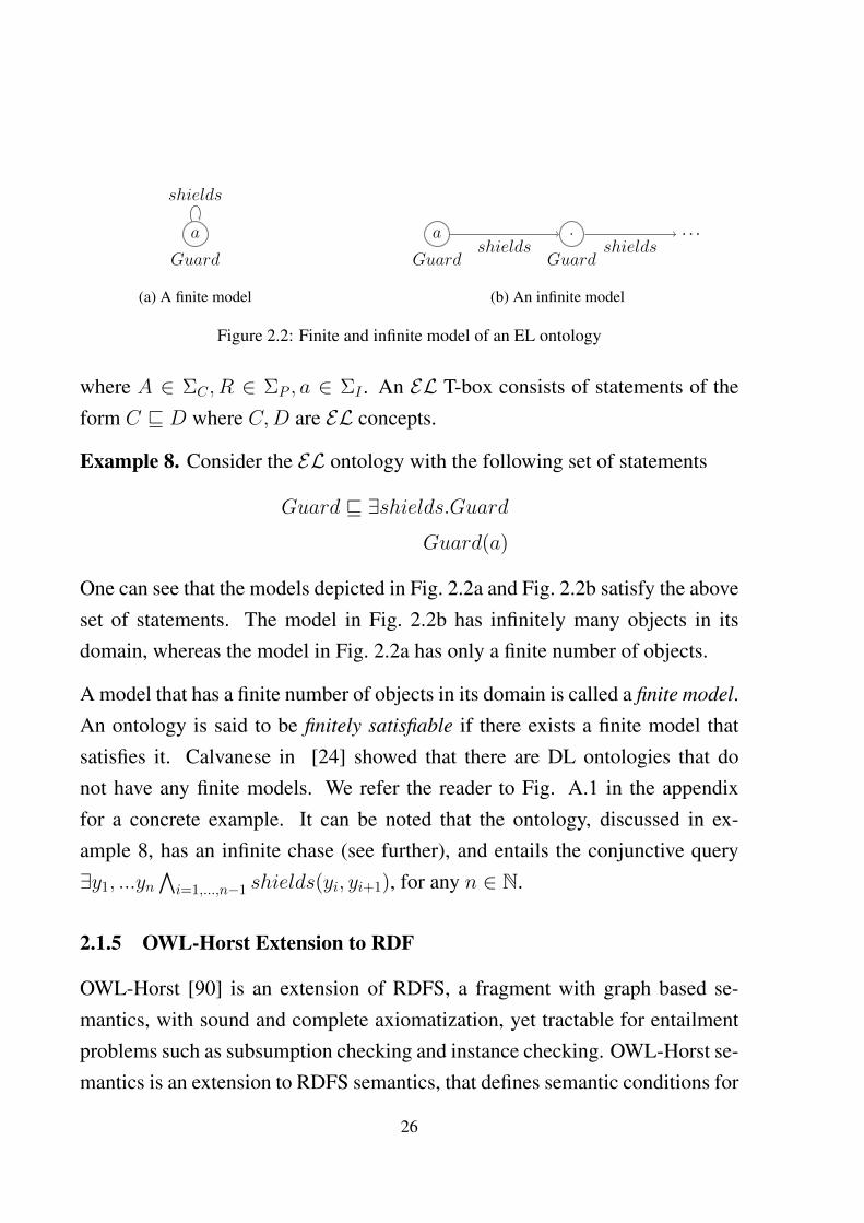
Figure 2.2: Finite and infinite model of an EL ontology

where A ∈ ΣC , R ∈ ΣP , a ∈ ΣI . An EL T-box consists of statements of theform C v D where C,D are EL concepts.

Example 8. Consider the EL ontology with the following set of statements

Guard v ∃shields.Guard

Guard(a)

One can see that the models depicted in Fig. 2.2a and Fig. 2.2b satisfy the aboveset of statements. The model in Fig. 2.2b has infinitely many objects in itsdomain, whereas the model in Fig. 2.2a has only a finite number of objects.

A model that has a finite number of objects in its domain is called a finite model.An ontology is said to be finitely satisfiable if there exists a finite model thatsatisfies it. Calvanese in [24] showed that there are DL ontologies that donot have any finite models. We refer the reader to Fig. A.1 in the appendixfor a concrete example. It can be noted that the ontology, discussed in ex-ample 8, has an infinite chase (see further), and entails the conjunctive query∃y1, ...yn

∧i=1,...,n−1 shields(yi, yi+1), for any n ∈ N.

2.1.5 OWL-Horst Extension to RDF

OWL-Horst [90] is an extension of RDFS, a fragment with graph based se-mantics, with sound and complete axiomatization, yet tractable for entailmentproblems such as subsumption checking and instance checking. OWL-Horst se-mantics is an extension to RDFS semantics, that defines semantic conditions for

26

a subset of terms in the OWL vocabulary. These include class assertions suchas OWL restrictions (universal, existential, value restrictions), disjointness ofclasses and properties, property assertions like symmetricity, transitivity, func-tionality, inverse relations of properties and assertions involving owl:sameAsand owl:differentFrom. Like RDF(S), any ontology serialized as a graphcan be interpreted using the OWL-Horst semantics. An OWL-Horst interpre-tation structure is an RDFS interpretation structure with additional semanticconstraints [90]. The class of OWL-Horst interpretation structures are hencea subset of the class of RDFS interpretation structures. OWL-Horst has a setof inference rules that are sound and complete w.r.t. its semantics, s.t. for anyOWL-Horst graph g, its deductive closure, owl-horst-closure(g), can be com-puted by repeatedly running the set of OWL-Horst inference rules on g until afix-point is reached, which is guaranteed to exist and is finite. OWL-Horst rea-soning for a graph can be characterized with the help of an OWL-Horst canon-

ical model, which is an OWL-Horst model that represents all the OWL-Horstmodels of a graph, and is defined as:

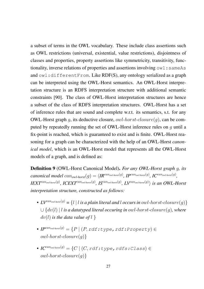
Definition 9 (OWL-Horst Canonical Model). For any OWL-Horst graph g, its

canonical model canowl-horst(g) = 〈IRcanowl-horst(g), IPcanowl-horst(g), ICcanowl-horst(g),

IEXTcanowl-horst(g), ICEXTcanowl-horst(g), IScanowl-horst(g), LVcanowl-horst(g)〉 is an OWL-Horst

interpretation structure, constructed as follows:

• LVcanowl-horst(g) = {l | l is a plain literal and l occurs in owl-horst-closure(g)}∪ {dv(l) | l is a datatyped literal occuring in owl-horst-closure(g), where

dv(l) is the data value of l }

• IPcanowl-horst(g) = {P | (P,rdf:type,rdf:Property) ∈owl-horst-closure(g)}

• ICcanowl-horst(g) = {C | (C,rdf:type,rdfs:Class) ∈owl-horst-closure(g)}

27

• IRcanowl-horst(g) = LVcanowl-horst(g) ∪ IPcanowl-horst(g) ∪ ICcanowl-horst(g) ∪ {a | (a,

rdf:type, rdfs:Resource ) ∈ owl-horst-closure(g)}

• IScanowl-horst(g) = {(a, a) | a is any URI, blank node or plain literal that

occurs in owl-horst-closure(g)} ∪ {(l, dv(l))|l is a datatyped literal oc-

curing in owl-horst-closure(g), whose data value is dv(l) }

• for every P ∈ IPcanowl-horst(g), IEXTcanowl-horst(g)(P ) = {(s, o) | (s, P, o) ∈owl-horst-closure(g)}

• for everyC ∈ ICcanowl-horst(g), ICEXTcanowl-horst(g)(C) = {a | (a,rdf:type, C)

∈ owl-horst-closure(g)}

Consistency as defined in [90], for an OWL-Horst graph, determines if thegraph has clashes or not. A clash, denoted by the symbol FALSE, can resultfrom invalid datatyped literals, or from simultaneous presence of conflictingstatements such as (a, owl:sameAs, b) and (a, owl:differentFrom, b).A graph g is said to be OWL-Horst inconsistent, if g |=owl-horst FALSE, andotherwise said to be OWL-Horst consistent. For any two OWL-Horst consistentgraphs g, h, the following are true:

• canowl-horst(g) |=owl-horst g

• canowl-horst(g) can be computed in PTIME

• g |=owl-horst h iff canowl-horst(g) |=simple h.

The proofs of these facts can be found in Horst [90].

2.1.6 Translations of OWL Statements to First Order Logic Statements

Note that any OWL statement (or an RDF statement) can be translated to a first-order logic sentence. The function Tx given in Table 2.2 defines the first-ordertranslation of common DL-constructs.

28

DL-construct Tx

A A(x)

∀R.C ∀y.R(x, y)→ Ty(C)

∃R.C ∃y.R(x, y) ∧ Ty(C)

¬C ¬Tx(C)

≥ nR.C ∃y1, ..., yn.R(x, y1) ∧ ... ∧ R(x, yn) ∧∧

i=1,...,n Tyi(C) ∧

∧1≤i6=j≤n yi 6= yj

≤ n− 1R.C ∃y1, ..., yn.R(x, y1) ∧ ... ∧ R(x, yn) ∧∧

i=1,...,n Tyi(C)→

∨1≤i6=j≤n yi = yj

∃R.self R(x, x)

p.s. y is a fresh variable, and R is an atomic role

Table 2.2: First order translation of DL concepts

C v D ∀x.Tx(C)→ Tx(D)

R v S ∀x, y.R(x, y)→ S(x, y)

C(a) C(a)

R(a, b) R(a, b)

Table 2.3: First order translation of DL statements for DLs with simple roles

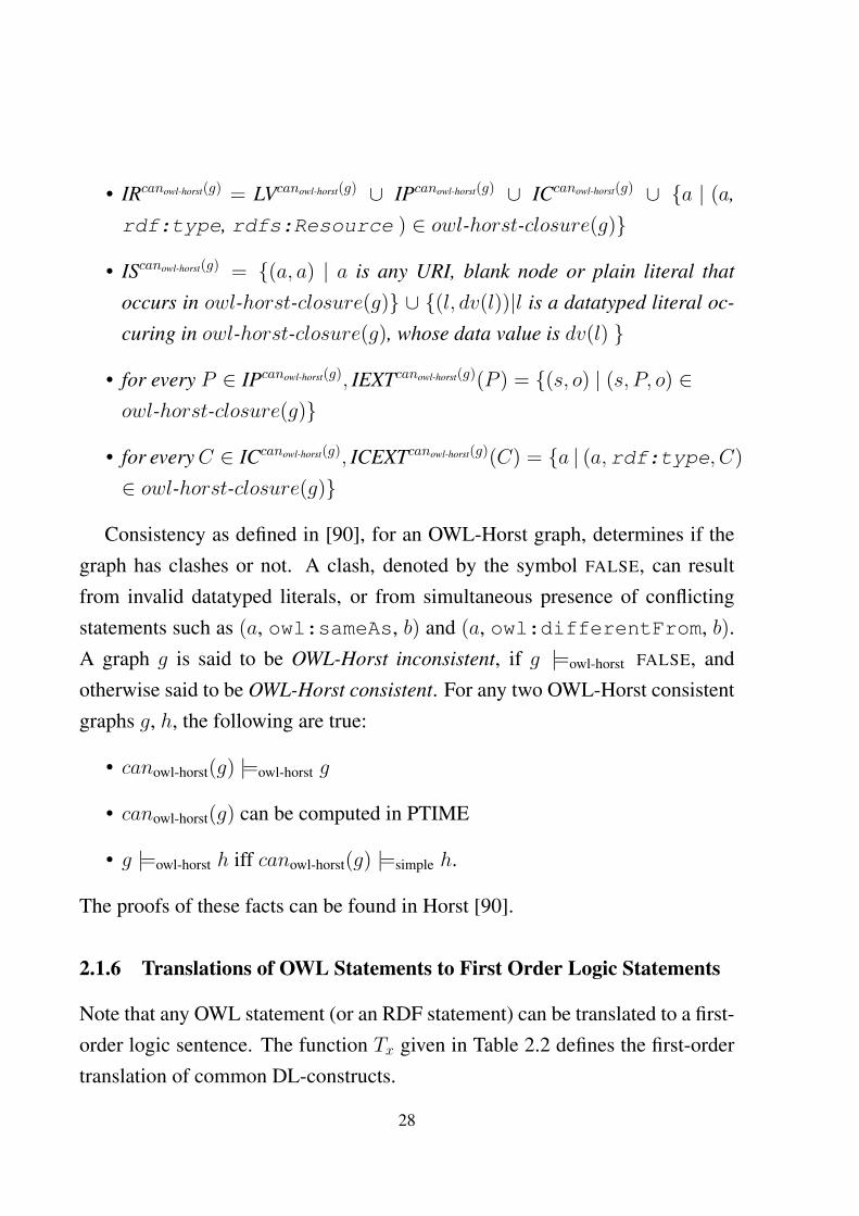
Example 10. consider the EL T-box statement

A u ∃R.B v ∃S.C uD

where A,B,C,D ∈ ΣC , R, S ∈ ΣP . Now using the translation given in table2.3, one can obtain:

∀x [A(x) ∧ ∃z(R(x, z) ∧B(z))→ ∃y (S(x, y) ∧ C(y)) ∧D(x)]

since y is free for A and y free for D, extending their scope results in

∀x [∃z(A(x) ∧R(x, z) ∧B(z))→ ∃y (S(x, y) ∧ C(y) ∧D(x))]

which can be written as

∀x [¬∃z(A(x) ∧R(x, z) ∧B(z)) ∨ ∃y (S(x, y) ∧ C(y) ∧D(x))]

which implies

∀x∀z [¬(A(x) ∧R(x, z) ∧B(z)) ∨ ∃y (S(x, y) ∧ C(y) ∧D(x))]

which can be written to the form described before:

∀x∀z [(A(x) ∧R(x, z) ∧B(z))→ ∃y (S(x, y) ∧ C(y) ∧D(x))]

Note that OWL profiles such as EL, QL, RL are fragments of a larger family ofDLs called Horn DLs [63]. Any Horn DL ontology has a unique chase, and canbe translated to a semantically equivalent set of forall-existential rules [32].

29

2.1.7 Forall-Existential (∀∃) Rules

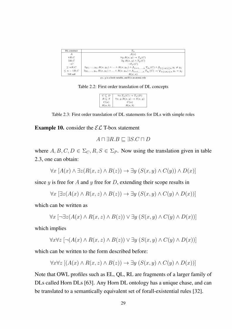
∀∃ rules (also known as Datalog+- rules [20] or tuple generating dependencies(tgds) [12]), a fragment of first order logic, is a popular language used for de-scribing ontologies in a rule based format. A field that is currently of extensiveresearch interest has given rise to large number of ∀∃ classes of varying compu-tational complexity. Besides, the RuleML initiative and its recently developedlanguage RuleLog3 is gaining popularity in the SW communities as a rule basedKR language, and has its foundations from ∀∃ rules. For any vector or sequence~x, we denote by ‖~x‖ the number of symbols in ~x, and by {~x} the set of symbolsin ~x. A ∀∃ rule is a first order formula of the form:

∀~x∀~z [p1(~x, ~z) ∧ ... ∧ pn(~x, ~z)→ ∃~y p′1(~x, ~y) ∧ ... ∧ p′m(~x, ~y)] (2.1)

where ~x, ~y, ~z are vectors of variables s.t. {~x}, {~y} and {~z} are pairwise disjoint,pi(~x, ~z), for 1 ≤ i ≤ n are predicate atoms whose variables are from ~x or ~z,p′1(~x, ~y), for 1 ≤ i ≤ m are predicate atoms whose variables are from ~x or~y. Sometimes, we write a ∀∃ rule r as φ(r)(~x, ~z) → ψ(r)(~x, ~y), or φ(~x, ~z)

→ ψ(~x, ~y), when r is implicit from the context. Also note φ(r)(~x, ~z) = φ(~x,~z) = {p1(~x, ~z), ..., pn(~x, ~z)}, ψ(~x, ~y)(r) = ψ(~x, ~y) = {p′1(~x, ~y), ... p′m(~x, ~y)}.A set of ∀∃ rules is called a ∀∃ rule set. Checking entailment over ∀∃ rulesets is undecidable, in general [12]. Various decidable subclasses with associ-ated entailment procedures have been derived lately. A few examples of thesesubclasses are the linear ∀∃ rules [56], (weakly) guarded rules [21], (weakly)frontier guarded rules [6], jointly frontier guarded rules [60], ‘sticky’ rules [23],and weakly acyclic rules [39, 34].

3http://ruleml.org/rif/rulelog/spec/Rulelog.html

30

2.2 Query Answering over Ontologies

Let V be the set of variables, any element of the set CV = V∪C is a term. Any(s, p, o) ∈ CV ×CV ×CV is called a triple pattern. A triple pattern t, whosevariables are elements of the vector ~x or ~y is written as t(~x, ~y). For any functionf : A→ B, the restriction of f to a set A′, is the mapping f |A′ from A′∩A toBs.t. f |A′(a) = f(a), for each a ∈ A∩A′. For any triple pattern t = (s, p, o) anda function µ from V to a set A, t[µ] denotes (µ′(s), µ′(p), µ′(o)), where µ′ is anextension of µ to C s.t. µ′|C is the identity function. For any set of triple patternsG, G[µ] denotes

⋃t∈G t[µ]. For any vector of constants ~a = 〈a1, . . . , a‖~a‖〉, and

vector of variables ~x of the same length, ~x/~a is the function µ s.t. µ(xi) = ai,for 1 ≤ i ≤ ‖~a‖. We use the notation t(~a, ~y) to denote t(~x, ~y)[~x/~a].

In this discussion, we limit ourselves to the class of Conjunctive queries

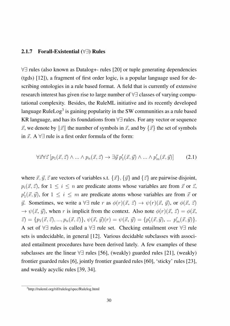
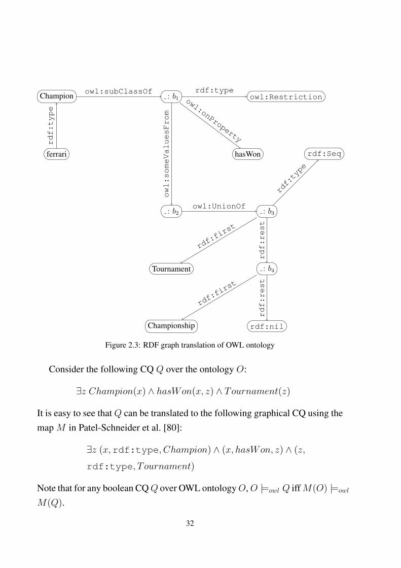
(CQ), which are also called select-project-join queries. It is well known thatmost of the queries that users pose to DBs/knowledge bases (KBs) are CQs. Theonly logical operators in CQs are conjunctions and existential quantifiers, andthey do not contain negations, universal quantification, or functional symbols.Since any OWL ontology serialized in a non-graphical syntax (for instance, infunctional style) can be translated using the standard map provided in Patel-Schneider et al.[80], and represented as a graph in RDF/XML syntax, and anyCQ over an OWL ontology can be translated to a graphical CQ (conjunct oftriple patterns) using the same map, we limit ourselves to graphical CQs.

Example 11. Consider an OWL ontology O whose statements in DL style syn-tax is as follows:

Champion v ∃ hasWon. Tournament t Championship

Champion(ferrari)

The mapping of O obtained by the standard OWL to RDF mapping M givenin Patel-Schneider et al. [80] is as shown in Fig 2.3. Note that the : b1, : b2,: b3, : b4 are auxilliary blank nodes introduced in the translation.

31

Champion

ferrari

: b1 owl:Restriction

hasWon

: b2 : b3

rdf:Seq

Tournament : b4

Championship rdf:nil

rdf:type

owl:subClassOf rdf:typeowl:onProperty

owl:someValuesFrom

owl:UnionOf

rdf:type

rdf:first

rdf:rest

rdf:first

rdf:rest

Figure 2.3: RDF graph translation of OWL ontology

Consider the following CQ Q over the ontology O:

∃z Champion(x) ∧ hasWon(x, z) ∧ Tournament(z)

It is easy to see that Q can be translated to the following graphical CQ using themap M in Patel-Schneider et al. [80]:

∃z (x,rdf:type, Champion) ∧ (x, hasWon, z) ∧ (z,

rdf:type, T ournament)

Note that for any boolean CQQ over OWL ontologyO,O |=owl Q iffM(O) |=owl

M(Q).

32

Definition 12 (Conjunctive query(CQ)). A CQ Q(~x) is an expression of the

form: ∃~y t1(~x, ~y) ∧ ... ∧tp(~x, ~y), where ti(~x, ~y) are triple patterns over vectors

of free variables ~x and quantified variables ~y, for i = 1, ..., p. A CQ is called a

boolean CQ if it does not have any free variables.

Let ~a be a vector such that ai ∈ U ∪ L and ‖~x‖ = ‖~a‖; for any query Q(~x),~x/~a in Q(~x) is denoted by Q(~a). For any CQ Q(~x) and a vector ~a, with ‖~x‖ =

‖~a‖, Q(~a) is boolean. A vector ~a is an answer for Q(~x) w.r.t. an interpretationI = 〈∆I , .I〉, if there exists an assignment µ from the set of existential variables{~y} to the domain ∆I , s.t. I |= ti(~a, ~y)[µ], for every ti(~a, ~y) ∈ Q(~a). Avector ~a is called a certain answer for Q(~x) w.r.t. a graph g iff I |= Q(~a), forevery model I of g. For any graph g, a CQ CQ(~x), and a vector ~a, the decisionproblem (DP) of checking if g |= CQ(~a) is called the CQ entailment problem.Complexity of CQ entailment problem is NP-complete for RDFS [82]. Whereascomplexity for CQ answering is still an open problem for OWL 1 DL and OWL2 DL [51], and no sound, complete algorithms are known yet for deciding CQentailment.

2.2.1 Chase of an Ontology

In the literature, query answering over an ontology is often done by computingthe chase [27, 56, 1] of an ontology. A chase of an ontology is a deductive clo-sure of the ontology, and the algorithm that computes the chase is often referredto as the chase algorithm. For any ontologyO, its chase chase(O) is a universal

model [35] of the ontology, i.e. chase(O) |= O and for any model I of O, thereexists a homomorphism h from chase(O) to I . Hence, for any boolean CQQ(), O |= Q() iff chase(O) |= Q(). In the following, we show how the chaseof an ontology can be constructed for a ∀∃ rules ontology. The technique canbe straightforwardly extended to DLs such as OWL 2 EL, OWL 2 QL and otherfragment of Horn DLs (DLs for which a unique Herbrand model exist). For

33

disjunctive ∀∃ rules (extension of ∀∃ rules with disjunctive heads) and DLs thatpermit disjunctions on the right hand side of subsumptions, Deutsch et al. [35]showed that a chase set [35, 70] can be devised for deciding CQ entailment.Various versions of chases, adequate for different scenarios, have been derivedfor ∀∃ rule sets. We now summarize each of these.

Oblivious chase For any ∀∃ rule r of the form ( 2.1), with slight abuse (Datalognotation) we write r as:

p1(~x, ~z), ..., pn(~x, ~z)→ p′1(~x, ~y), ..., p′m(~x, ~y) (2.2)

Let Bsk be a fresh set of blank nodes called Skolem blank nodes. For any ∀∃rule r of the form ( 2.2), and an assignment µ : {~x} ∪ {~z} → C, the functionapply(r, µ) is defined as follows:

apply(r, µ) = head(r)[µext(~y)]

where µext(~y) is an extension of µ s.t. µext(~y)(yi) is a distinct fresh Skolem blanknode from Bsk, for each yi ∈ {~y}. For any ∀∃ rule r of the form ( 2.2), a setof instances A, and an assignment µ : {~x} ∪ {~z} → C, the boolean functionOapplicable(r, µ, A) is defined as follows:

Oapplicable(r, µ, A) =

{True, if body(r)[µ] ⊆ A;

False, Otherwise;

For any ∀∃ rule set R, a set of instances A, let

OΣ(R,A) = {(r, µ)|Oapplicable(r, µ, A) = True}

LetOchase0(R) = {ψ(~x, ~y)|r =→ ψ(~x, ~y) ∈ R};

for i ∈ N,

Ochasei+1(R) = Ochasei(R) ∪⋃

(r,µ)∈OΣ(R,Ochasei(R))

apply(r, µ)

34

The oblivious chase of R, denoted Ochase(R), is given as:

Ochase(R) =⋃i∈N

Ochasei(R)

We say that two sets of instances A and B are equivalent, denoted A ≡ B,iff there exists homomorphisms h1 and h2 s.t. A[h1] ⊆ B and B[h2] ⊆ A.Intuitively, Ochasei(R) can be thought of as the state of Ochase(R) at the endof iteration i. In the oblivious case, the termination condition is given by:If ∃i s.t. Ochasei(R) ≡ Ochasei+1(R), then Ochase(R) = Ochasei(R);Hence, an algorithm that computes the oblivious chase, at each iteration, needsto take the overhead of checking equivalence of current chase state with theprevious chase state. Note that complexity of checking equivalence of two setsof instances is worst case exponential in the size of instances.

Skolem chase We now show how the Skolem chase given in works such as Mar-nette [69] and Cuenca Grau et al [32] is constructed. For any ∀∃ rule r of theform (2.1), the skolemization sk(r) is the result of replacing each yi ∈ {~y} witha globally unique Skolem function f ri , s.t. f ri : C‖~x‖→ Bsk. Intuitively, for ev-ery distinct vector ~a of constants, with ‖~a‖ = ‖~x‖, f ri (~a) is a fresh blank node,whose node id is a hash of ~a. Let ~f r = 〈f r1 , ..., f r‖~y‖〉 be a vector of distinctSkolem functions; For any ∀∃ rule r the form (2.1), with slight abuse we writeits skolemization sk(r) as follows:

p1(~x, ~z), ..., pn(~x, ~z)→ p′1(~x,~f r), ..., p′m(~x, ~f r) (2.3)

Moreover, any skolemized ∀∃ rule r of the form (2.3) can be replaced by thefollowing equivalent set of formulas, whose size is worst case quadratic w.r.tthe size of r:

{p1(~x, ~z), ..., pn(~x, ~z)→ p′1(~x,~f r), (2.4)

...,

p1(~x, ~z), ..., pn(~x, ~z)→ p′m(~x, ~f r)}

35

Note that each BR in the above set has exactly one predicate atom with optionalfunction symbols in the head. Also note that a ∀∃ rule without function symbolscan be replaced with a set of ∀∃ rules with single atom heads. Hence, w.l.o.g,we assume that any ∀∃ rule in a skolemized set sk(R) of ∀∃ rules is of the form(2.4).

For any set of instances A and a skolemized ∀∃ rule r of the form (2.4), theapplication of r on A, denoted by r(A), is given as:

r(A) =⋃

µ∈V→C

{p′1(~x,

~f r)[µ] | p1(~x, ~z)[µ] ∈ A, ..., pn(~x, ~z)[µ] ∈ A}

For any set of skolemized ∀∃ rules R, application of R on A is given by:

R(A) =⋃r∈R

r(A)

For any ∀∃ rule set R, generating BRs RF is the set of BRs in sk(R) withfunction symbols, and the non-generating BRs is the set RI = sk(R) \RF .Let

Schase0(R) = {ψ(~x, ~f)|r =→ ψ(~x, ~f) ∈ sk(R)};

for i ∈ N, Schasei+1(R) =

Schasei(R) ∪RI(Schasei(R)), if RI(Schasei(R)) 6⊆ Schasei(R);

Schasei(R) ∪RF (Schasei(R)), otherwise;

The Skolem chase of R, denoted Schase(R), is given as:

Schase(R) =⋃i∈N

Schasei(R)

Intuitively, Schasei(R) can be thought of as the state of Schase(R) at the end ofiteration i. In the Skolem case, the termination condition is simpler and is givenby: If ∃i s.t. Schasei(R) = Schasei+1(R), then Schase(R) = Schasei(R).Note that if the Skolem chase of an ontology terminates, then so does the re-stricted chase and the core chase of the ontology [32].

36

Core chase The core chase is a slight variant of the oblivious chase in which thecore of the chase results are computed at each iteration. For a set of instancesA, its core core(A) is a minimal subset of A that is equivalent to A [6]. Notethat multiple cores of a set of instances are (homomorphically) equivalent [35].Let

Cchase0(R) = core(Ochase0(R));

for i ∈ N,

Cchasei+1(R) = core(Cchasei(R) ∪⋃

(r,µ)∈OΣ(R,Cchasei(R))

apply(r, µ))

The core chase of R, denoted Cchase(R), is given as:

Cchase(R) =⋃i∈N

Cchasei(R)

Intuitively, Cchasei(R) can be thought of as the state of Cchase(R) at the endof iteration i. The termination condition is given by:If ∃i s.t. Cchasei(R) ≡ Cchasei+1(R), then Cchase(R) = Cchasei(R);An algorithm that computes the core chase, at each iteration, needs to takethe overhead of checking equivalence of current chase state with the previouschase state. Note that, for any rule set R, for each i ∈ N, Cchasei(R) =

core(Ochasei(R)).

Non-oblivious/Restricted chase The restricted chase (also called non-obliviouschase) given in Fagin et al. [39] is a version of the chase in which a redun-dancy check is performed before rule application. A rule is only applied, if therule application is not redundant, i.e. the application of the rule does not lead toan equivalent set.

Assume that there exists a strict linear order ≺ that linearly orders the setof all instance sets. Cali et al [21] gives one such order based on lexicographicorder of the constants. Also for any two rules r, r′ and assignments µ, µ′, let(r, µ) ≺ (r′, µ′) iff φ(r)[µ] ≺ φ(r′)[µ′].

37

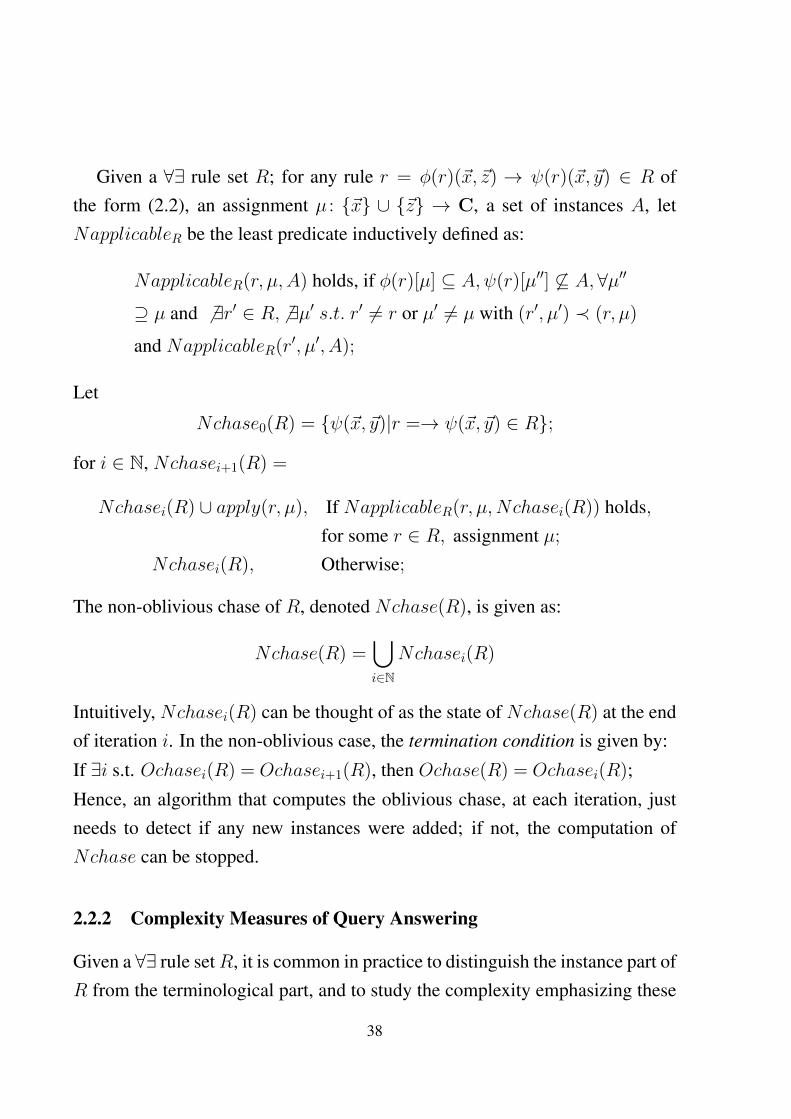
Given a ∀∃ rule set R; for any rule r = φ(r)(~x, ~z) → ψ(r)(~x, ~y) ∈ R ofthe form (2.2), an assignment µ : {~x} ∪ {~z} → C, a set of instances A, letNapplicableR be the least predicate inductively defined as:

NapplicableR(r, µ, A) holds, if φ(r)[µ] ⊆ A,ψ(r)[µ′′] 6⊆ A, ∀µ′′

⊇ µ and 6 ∃r′ ∈ R, 6 ∃µ′ s.t. r′ 6= r or µ′ 6= µ with (r′, µ′) ≺ (r, µ)

and NapplicableR(r′, µ′, A);

Let

Nchase0(R) = {ψ(~x, ~y)|r =→ ψ(~x, ~y) ∈ R};

for i ∈ N, Nchasei+1(R) =

Nchasei(R) ∪ apply(r, µ), If NapplicableR(r, µ,Nchasei(R)) holds,for some r ∈ R, assignment µ;

Nchasei(R), Otherwise;

The non-oblivious chase of R, denoted Nchase(R), is given as:

Nchase(R) =⋃i∈N

Nchasei(R)

Intuitively, Nchasei(R) can be thought of as the state of Nchase(R) at the endof iteration i. In the non-oblivious case, the termination condition is given by:

If ∃i s.t. Ochasei(R) = Ochasei+1(R), then Ochase(R) = Ochasei(R);

Hence, an algorithm that computes the oblivious chase, at each iteration, justneeds to detect if any new instances were added; if not, the computation ofNchase can be stopped.

2.2.2 Complexity Measures of Query Answering

Given a ∀∃ rule setR, it is common in practice to distinguish the instance part ofR from the terminological part, and to study the complexity emphasizing these

38

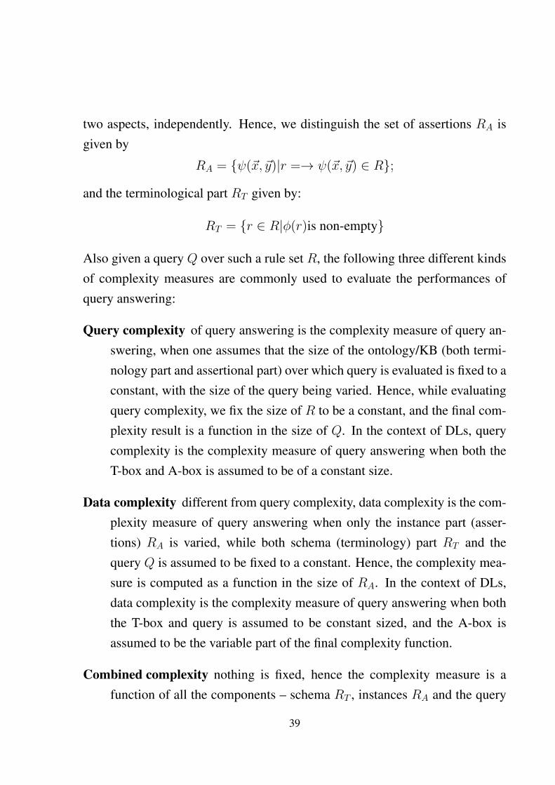
two aspects, independently. Hence, we distinguish the set of assertions RA isgiven by

RA = {ψ(~x, ~y)|r =→ ψ(~x, ~y) ∈ R};

and the terminological part RT given by:

RT = {r ∈ R|φ(r)is non-empty}

Also given a query Q over such a rule set R, the following three different kindsof complexity measures are commonly used to evaluate the performances ofquery answering:

Query complexity of query answering is the complexity measure of query an-swering, when one assumes that the size of the ontology/KB (both termi-nology part and assertional part) over which query is evaluated is fixed to aconstant, with the size of the query being varied. Hence, while evaluatingquery complexity, we fix the size of R to be a constant, and the final com-plexity result is a function in the size of Q. In the context of DLs, querycomplexity is the complexity measure of query answering when both theT-box and A-box is assumed to be of a constant size.

Data complexity different from query complexity, data complexity is the com-plexity measure of query answering when only the instance part (asser-tions) RA is varied, while both schema (terminology) part RT and thequery Q is assumed to be fixed to a constant. Hence, the complexity mea-sure is computed as a function in the size of RA. In the context of DLs,data complexity is the complexity measure of query answering when boththe T-box and query is assumed to be constant sized, and the A-box isassumed to be the variable part of the final complexity function.

Combined complexity nothing is fixed, hence the complexity measure is afunction of all the components – schema RT , instances RA and the query

39

Q. In case of DLs, all the components T-box, A-box and query are consid-ered to be variant while analyzing combined complexity.

2.3 Computational Complexity Fundamentals

In the following, we give an overview of basic notions of computational com-plexity, necessary for grasping the complexity intricacies of this thesis. For adetails on these topics, we refer the readers to books such as Goldreich [44] andArora et al. [3].

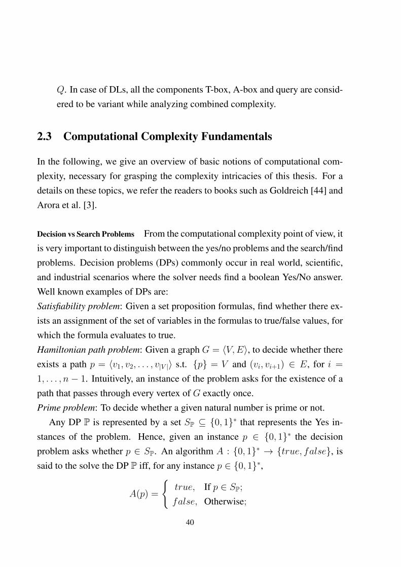
Decision vs Search Problems From the computational complexity point of view, itis very important to distinguish between the yes/no problems and the search/findproblems. Decision problems (DPs) commonly occur in real world, scientific,and industrial scenarios where the solver needs find a boolean Yes/No answer.Well known examples of DPs are:Satisfiability problem: Given a set proposition formulas, find whether there ex-ists an assignment of the set of variables in the formulas to true/false values, forwhich the formula evaluates to true.Hamiltonian path problem: Given a graph G = 〈V,E〉, to decide whether thereexists a path p = 〈v1, v2, . . . , v|V |〉 s.t. {p} = V and (vi, vi+1) ∈ E, for i =

1, . . . , n − 1. Intuitively, an instance of the problem asks for the existence of apath that passes through every vertex of G exactly once.Prime problem: To decide whether a given natural number is prime or not.

Any DP P is represented by a set SP ⊆ {0, 1}∗ that represents the Yes in-stances of the problem. Hence, given an instance p ∈ {0, 1}∗ the decisionproblem asks whether p ∈ SP. An algorithm A : {0, 1}∗ → {true, false}, issaid to the solve the DP P iff, for any instance p ∈ {0, 1}∗,

A(p) =

{true, If p ∈ SP;

false, Otherwise;

40

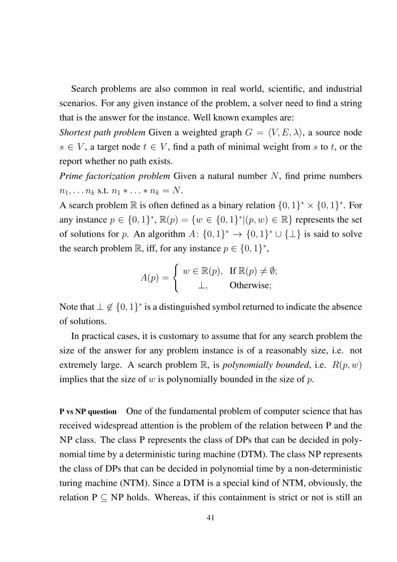
Search problems are also common in real world, scientific, and industrialscenarios. For any given instance of the problem, a solver need to find a stringthat is the answer for the instance. Well known examples are:

Shortest path problem Given a weighted graph G = 〈V,E, λ〉, a source nodes ∈ V , a target node t ∈ V , find a path of minimal weight from s to t, or thereport whether no path exists.

Prime factorization problem Given a natural number N , find prime numbersn1, . . . nk s.t. n1 ∗ . . . ∗ nk = N .

A search problem R is often defined as a binary relation {0, 1}∗ × {0, 1}∗. Forany instance p ∈ {0, 1}∗, R(p) = {w ∈ {0, 1}∗|(p, w) ∈ R} represents the setof solutions for p. An algorithm A : {0, 1}∗ → {0, 1}∗ ∪ {⊥} is said to solvethe search problem R, iff, for any instance p ∈ {0, 1}∗,

A(p) =

{w ∈ R(p), If R(p) 6= ∅;⊥, Otherwise;

Note that⊥ 6∈ {0, 1}∗ is a distinguished symbol returned to indicate the absenceof solutions.

In practical cases, it is customary to assume that for any search problem thesize of the answer for any problem instance is of a reasonably size, i.e. notextremely large. A search problem R, is polynomially bounded, i.e. R(p, w)

implies that the size of w is polynomially bounded in the size of p.

P vs NP question One of the fundamental problem of computer science that hasreceived widespread attention is the problem of the relation between P and theNP class. The class P represents the class of DPs that can be decided in poly-nomial time by a deterministic turing machine (DTM). The class NP representsthe class of DPs that can be decided in polynomial time by a non-deterministicturing machine (NTM). Since a DTM is a special kind of NTM, obviously, therelation P ⊆ NP holds. Whereas, if this containment is strict or not is still an

41

open problem, often referred to as the P vs NP question. According to an alter-nate equivalent definition of NP [44], the class NP refers to the class of decisionproblems for which there exists a polynomial time proof procedure. That is, forany DP P in NP, there exists a polynomial time procedure A, s.t. if p in the setof Yes instances of P, i.e. if p ∈ SP, then there exists a polynomial sized stringw, called the NP-proof s.t. A(p, w) = true. A DP P is in class P, iff there existsa polynomial time procedureA s.t. for any instance p, p is in the Yes instance ofP, i.e. p ∈ SP, iff A(p) = true. Hence, P vs NP question also put forwards thequestion of whether or not the existence of (reasonably sized) proofs adds to theefficiency in computation. The unsettled variations of the question arises alsowhen considering higher classes of computation, and give rise to: EXPTIME vsNEXPTIME, 2EXPTIME vs 2NEXPTIME, and so on.

Undecidability/Unsolvability of Problems A decision problem P is called decidableiff there exists an algorithm A that decides the membership in the set SP, i.e forany instance p ∈ {0, 1}∗

A(p) =

{true, If p ∈ SP;

false, Otherwise;

A problem in undecidable, iff it is not decidable. The set of inputs to functionscorresponds to the set N of natural numbers. Since any decision problem can beseen as a function that that an inputs a natural number, and returns 0 or 1. Thecardinality of set of problems correspond to the set of all (boolean) functions,N → {0, 1}, which is equal to 2N. Since any program has a description thatcan be seen as a natural number, The set of programs corresponds to the naturalnumbers. It is well known that 2N is strictly greater than N, the cardinality ofdecision problems are strictly higher than the cardinality of programs. Hence,there should be DPs for which there can not exist programs that decide them.

Example 13. An example of an undecidable problem is the halting problem.

42

The halting problem H is the following two argument function:

H(n1, n2) =

{true, If program n1 on input n2 halts;false, Otherwise;

where n1, n2 ∈ N. Cantor, the renowned computer scientist with a diagonaliza-tion argument showed that halting problem is undecidable.

Complexity Classes Below, we briefly overview some of the well known com-plexity classes, some of which are used henceforth. The following containmentrelation between classes are well known:

AC0 ( LOGSPACE ⊆ NLOGSPACE ⊆ PTIME ⊆ NP

⊆ EXPTIME ⊆ NEXPTIME ⊆ 2EXPTIME

Also the following strict containment relations are known:

PTIME ( EXPTIME ( 2EXPTIME

The class AC0 is based on the circuit model of complexity. A (decision)problem belongs to AC0 if it can be decided in constant time by a circuit that haspolynomial number of gates w.r.t the size of the input. An example of a problemthat is in AC0 from the DB/KR context is the data complexity of answering firstorder queries over relational DBs. The class LOGSPACE represents the class of(decision) problems that can be decided by a 2-tape DTM, that receives its inputstring on the read-only input tape, and uses only space of the read-write worktape that is at most logarithmic w.r.t to the input size. The class NLOGSPACE issimilar, except that a non-deterministic turing machine is assumed instead of adeterministic one. A typical problem that is in LOGSPACE (but not in AC0) isundirected-graph reachability, i.e. the problem of determining if a target nodeis reachable from a source node in an undirected graph. Similarly, a typicalproblem that is in NLOGSPACE is directed-graph reachability.

43

A problem is called hard for a class, if every other problem in the class isreducible to the problem in a reasonably small amount of time. Polynomialtime reductions and logspace reductions are the commonly considered ones. Aproblem is called complete for a class, if the problem is hard for the class andis also a member of the class. Well known problems that are complete for classNP, are the boolean satisfiability problem, graph homomorphism problem, andthree colorability problem of undirected graphs. Well known problem that iscomplete for class P is Horn-Sat, the satisfiability problem of propositional hornclauses.

44

Chapter 3

Contextual Representation and Reasoningfor Semantic Web: A Review on ExistingFrameworks

In this chapter, we review some of the well known existing frameworks, inthe SW area, for reasoning with contextualized knowledge. An attempt to for-malize contexts was done by McCarthy [55] in the realm of AI, as early as inthe 80s. The main solution proposed by McCarthy was to consider contextsas first-class objects, apart from standard logical primitives; his proposal con-sisted of a special predicate ist using which one could specify axioms such asist(c, ∀x.person(x) → smart(x)), to intuitively mean that “every person inthe scope of context c is smart”. Lifting rules were used to import/inter-operateaxioms between contexts. As pointed out by Guha et al. [45] and Bouquet etal. [81], the intricacy of these and the other mechanisms of contexts that existedin AI was not directly applicable for SW applications. As a result a numberof works appeared in the 2000s, particularly focusing on problems related tocontexts from the SW perspective. In the following, we review some of theimportant ones:

45

3.1 Distributed Description Logics

Distributed Description Logic (DDL) [14], proposed by Borgida and Serafini,was one of the pioneers among the frameworks for representation of contextual-ized knowledge in the SW setting. The original work, proposed as an extensionto description logics, was motivated to reason with a distributed set of infor-mation sources, s.t. each of these sources could assimilate knowledge from theother sources. In DDL each of these information source is a DL KB, and sincethe information sources model domains that can have possible interconnections,bridge rules and individual correspondences are provided for interoperability ofthe distributed KBs.

Given two DL languages Li and Lj, a bridge rule from i to j is an expressionof one of the following forms:

i : Av−→ j : B, called into-bridge rule

i : Aw−→ j : B, called onto-bridge rule

Intuitively, the into-bridge states that according to information source j, theobjects of type A in information source i are of type B in information sourcei. Whereas, an onto-bridge rule states that according to the information sourcej, every object of type B is also of type A in the information source i. Anindividual correspondence is an expression of the form:

i : a 7→ j : b

where a and b are instances of DL languages Li and Lj, respectively, and intu-itively means that according to information source j its object b is same as theobject a in information source i.

Definition 1. Given a set I of indices, let {Li}i∈I be a collection of DL lan-

guages. A distributed T-box T = 〈{Ti}i∈I ,B〉 consists of a set of ordinary DL

T-boxes {Ti}i∈I , and a set B = {Bij}i6=j∈I of bridge rules. For every k ∈ I , all

46

the assertions in Tk should be in the corresponding DL language Lk. And, for

every bridge rule i : A v−→ j : B or i : A w−→ j : B in Bij, the concepts A and

B must be in Li and Lj, respectively.

A distributed A-box A = 〈{Ai}i∈I ,C〉 consists of a a set of A-boxes {Ai}i∈I ,and a set C = {Cij}i6=j∈I of individual correspondences. For every k ∈ I , all

descriptions in Ak must be in the corresponding language Lk, and for every

correspondence of the form i : a 7→ j : b, the individuals a and b must be in

languages Li and Lj, respectively.

A DDL KB is a pair 〈T, A〉, consisting of a distributed T-box T and a dis-

tributed A-box A.

DDL semantics is defined on top of a distributed interpretation (structure),which is a set of local DL interpretation structures, one each for each individualinformation system, which are further connected by domain relation mappings.

Definition 2. A distributed interpretation structure I = 〈{Ii}i∈I , r〉 consists of

DL interpretation structures Ii = 〈∆Ii, ·Ii〉, and a set of relations r = {rij}i6=j∈I ,where rij ⊆ ∆i ×∆j.

Satisfaction of distributed T-box statements are defined as follows:

Definition 3. A distributed interpretation I = 〈{Ii}i∈I , r〉, d-satisfies (elements

of) a distributed T-box T = 〈{Ti}i∈I ,B〉 (written I |=d), is given as per the

following conditions:

• I |=d i : Av−→ j : B, iff rij(AIi) ⊆ BIj ,

• I |=d i : Aw−→ j : B, iff rij(AIi) ⊇ BIj ,

• I |=d i : A v B, iff Ii |=DL A v B,

• I |=d Ti, iff Ii |=DL Ti,

• I |=d T, iff I |=d Ti and I d-satisfies every bridge rule in B,

47

where i 6= j ∈ I and |=DL is the classical DL satisfaction relation.

Satisfaction of a distributed A-box is defined as follows:

Definition 4. A distributed interpretation I = {Ii}i∈I d-satisfies (elements of)

a distributed A-box A = 〈{Ai}i∈I ,C〉, is given as per the following conditions:

• I |=d i : a 7→ j : b, iff bIj ∈ rij(aIi),

• I |=d i : C(a), iff Ii |=DL C(a),

• I |=d i : P (a, b), iff Ii |=DL P (a, b),

• I |=d Ai, iff I |=d st, for every st ∈ Ai,

• I |=d A, iff I |=d Ai, for every i ∈ I , and I d-satisfies every individual

correspondence in C,

where i 6= j ∈ I and |=DL is the classical DL satisfaction relation.

A DDL KB KB d-entails DDL axiom st, iff every distributed model of KBsatisfies st. A DDL KB KB1 d-entails a DDL KB KB2, iff KB1 entails st, forevery st ∈ KB2.

Wide reach of DDL in SW community is manifested by numerous imple-mentation, application, and extension attempts. C-OWL by Bouquet et al. [15]proposes an extension of OWL language using the DDL semantics that enablesthe creation of ontologies with multiple local contexts. Also the authors showhow the hole interpretations, which are standard OWL interpretations in whichevery concept and role is empty, can be used to satisfy inconsistent contextsand prevent inconsistency propagation from a locally inconsistent context to alocally consistent context, in spite of the existence of mapping bridge rules. Theauthors also demonstrate how directionality of mappings can be achieved usinginto/onto bridge rules of DDL and the domain relations in the DDL semantics.DRAGO [87] is a robust extension of the Pellet DL reasoner [88] based on

48

Tableaux calculus that enables reasoning with DDL semantics over distributedontologies. Homola et al. [52] proposed an extension to DDL semantics withcompositionality property of subsumption axioms. Given

i : Cv−→ j : E and i : D v−→ j : F

then the compositionality constraint (which the plain DDL does not possess)ensures that

i : C �D v−→ j : E � F

where i, j are DL KBs, C,D are DL-concepts of language Li, E,F are DL-concepts of language Lj, � is any DL-Connective.

3.2 E-connections

E-connections [64] is a methodology for connecting multiple ontologies thatrepresents multiple contexts of a domain via the concept of ontology linking.These multiple ontologies could possibly be defined using multiple logical lan-guages. An example of an E-connections is a domain D1 of companies and lo-cations, connected to a domain D2 of people using the set of links E = {L,W},where L,W ⊆ D1 × D2. A pair (x, y) ∈ L, intuitively represents the factthat an individual y of D2 lives in a location x of D1, and a pair (x, y) ∈ W ,intuitively represents the fact that an individual y of D2 works in a company xin D1. The component domains are represented using the notion of an abstract

description system. Common language variants for describing systems such astemporal logics, spatial logics, description logics can be represented using anabstract description system.

Abstract Description System (ADS)

An abstract description language (ADL)L is determined by a countably infiniteset of set variables V , a countably infinite set of object variables X , a finite set

49

of relation symbols R, a finite set of function symbols F . For any R ∈ R andf ∈ F , let ar(R) and ar(f), denote the arity of R and f , respectively. Theterms tj of L are inductively built as follows:

tj := x | ¬t1 | t1 ∧ t2 | f(t1, ...tar(f))

where x ∈ V , f ∈ F . The term assertions of L are of the form t1 v t2, wheret1, t2 are terms, and the object assertions are of the form:

• R(a1, ..., aar(R)), for a1, ..., aar(R) ∈ X , R ∈ R;

• t(a), for a ∈ X and t a term.

The set of term assertions and object assertions together form the set of L-assertions.

The semantics of ADLs are defined via abstract description models. Givena ADL L = 〈V ,X ,R,F〉, an abstract description model (ADM) for L is astructure of the form:

M = 〈W,VM = {vM}v∈V ,XM = {aM}a∈X ,RM = {RM}R∈R,FM = {fM}f∈F〉,

where W is a non-empty set, vM ⊆ W , xM ∈ W , fM is function mappingar(f)-tuples 〈X1, ..., Xar(f)〉 of subsets of W to a subset of W , and the RM

are ar(R)-ary relations on W . The value tM ⊆ W of an L-term t is definedinductively as:

• (¬t)M = W \ tM,

• (t1 ∧ t2)M = tM1 ∩ tM2 ,

• (f(t1, ..., tar(f)))M = fM(tM1 , ..., t

Mar(f)).

The satisfaction relation M |= φ of an L-assertion φ is defined in the obviousway:

• M |= R(a1, ...aar(R), iff RM(aM1 , ..., aMar(R)),

50

• M |= t(a), iff aM ∈ tM,

• M |= t1 v t2, iff tM1 ⊆ tM2 ,

For a set γ of assertions, M |= γ iff M |= φ, for all φ ∈ γ.

Definition 5. An ADS is a pair 〈L,M〉, where L is an abstract description

language andM is a class of ADMs for L.

E-connections of Abstract Description Systems

Suppose we want to connect n ADSs S1, ...,Sn, Si = 〈Li,Mi〉 for 1 ≤ i ≤ n.In order to connect S1, ...,Sn, the following additional constructors are used:

1. a non-empty set of n-ary relational symbols

E = {Ej}j∈J ,

2. for 1 ≤ i ≤ n and each j ∈ J , function symbols 〈Ej〉i of arity n − 1 thatare distinct from functional symbols of S1, ...,Sn.

The elements of E are called link relations, (or links, for short) and the functionsymbols 〈Ej〉i, link operators.

The definition of E-connection CE(S1, ...,Sn) of S1, ...,Sn, following the def-inition of ADS, contains a set of terms of CE(S1, ...,Sn), assertions, and finally aclass of models and a satisfaction relation between these models and assertions.The set of CE(S1, ...,Sn)-terms is partitioned into n sets, each of which containsi-terms, for 1 ≤ i ≤ n. Intuitively, i-terms are the terms of Li enriched withnew function symbols 〈Ej〉i for each j ∈ J . They are defined inductively as:

• every set variable of Li is an i-term;

• the set of i-terms is closed under ∧,¬ and the function symbols of Li;

51

• if (t1, ..., ti−1, ti+1, ..., tn) is a sequence of k-terms tk for k 6= i, then

〈Ej〉i(t1, ..., ti−1, ti+1, ..., tn)

is an i-term, for every j ∈ J .

There are three types of assertions for CE(S1, ...,Sn). Two of these types arethe term assertions and the object assertions of component ADSs. Additionally,to be able to speak about the ingredients of E-connections, link relations, link

assertions are used. The set of assertions of CE(S1, ...,Sn) are defined as per thefollowing rules. For 1 ≤ i ≤ n,

• the i-term assertions are of the form t1 v t2, where both t1 and t2 arei-terms;

• the i-object assertions are of the form t(a) orR(a1, ..., aar(R)), where a anda1, ..., aar(R) are object variables of Li, t is an i-term, and R a relationalsymbols of Li;

• the link assertions are of the form Ej(a1, ...., an), where ai are object vari-ables of Li, 1 ≤ i ≤ n, and j ∈ J .

Taken together, the set of term assertions, object assertions and link asser-tions form the set of assertions of the E-connection CE(S1, ...,Sn). A finiteset of assertions is called a knowledge base of CE(S1, ...,Sn). The semantics ofCE(S1, ...,Sn) is defined using a structure of the form:

M = 〈{Mi}1≤i≤n, EM = {EMj }j∈J〉,

where Mi ∈ Mi, for 1 ≤ i ≤ n and EMj ⊆ (W1 × ... ×Wn), for each j ∈ J .

The extension tM of an i-term is defined inductively as per the following rules.For a set variable X and an object variable a of Li, XM = XMi and aM = aMi.For boolean and function symbols of Li:

• (¬t1)M = Wi \ tM1 , (t1 ∧ t2)M = tM1 ∩ tM2 ,

52

• (f(t1, ..., tar(f))M = fMi(tM1 , ..., t

Mar(f))

Now let ~ti = (t1, ..., ti−1, ti+1, ..., tn) be a sequence of j-terms tj, j 6= i. Then

(〈Ej〉i(~ti))M = {x ∈ Wi|∃l 6=ixl ∈ tMl .(x1, ..., xi−1, x, xi+1, ..., xn) ∈ EMj }

Finally the extension RM of a relational symbol R of Li is just RMi. The truthrelation |= between models M for CE(S1, ...,Sn) is defined in the obvious way:

• M |= t1 v t2 iff tM1 ⊆ tM2 ;

• M |= t(a) iff aM ∈ tM;

• M |= R(a1, ..., aar(R)) iff RM(aM1 , ..., aMar(R));

• M |= Ej(a1, ..., an) iff EMj (aM1 , ..., a

Mn ).

Example 6 (Description Logic-Spatial Logic). A description logic language L1

talks about a domain D1 of objects, and spatial logic language L2 talks about aspatial domain D2. An E-connection is a relation E ⊆ D1×D2 defined by tak-ing (x, y) ∈ E iff y belongs to the spatial extension of x – whenever x occupiessome space. Given a L1 concept, say university, the operator 〈E〉2(University)

provides us with the spatial extension of all universities. Conversely, given aspatial region say, Italy, 〈E〉1(Italy) provides us the concept comprising all theobjects, whose spatial extension has a non-empty intersection with Italy. So theconcept University u 〈E〉1(Italy) will then denote all the Italian universities.

Several extensions to E-connection frameworks have been proposed and im-plemented. One of the notable ones by Parsia et al. [78] extends the link prop-erties to those which support link properties that are transitive, or also holdbetween multiple pairs of ADSs/components. Also, the authors provide a deci-sion procedure based on Tableaux calculus for reasoning with E-connected DLsystems for expressive DLs such as SHIQ and SHOQ.

53

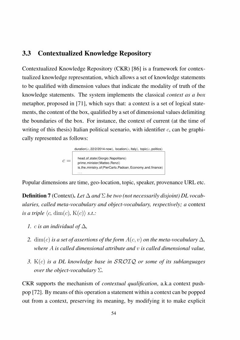
3.3 Contextualized Knowledge Repository

Contextualized Knowledge Repository (CKR) [86] is a framework for contex-tualized knowledge representation, which allows a set of knowledge statementsto be qualified with dimension values that indicate the modality of truth of theknowledge statements. The system implements the classical context as a box

metaphor, proposed in [71], which says that: a context is a set of logical state-ments, the content of the box, qualified by a set of dimensional values delimitingthe boundaries of the box. For instance, the context of current (at the time ofwriting of this thesis) Italian political scenario, with identifier c, can be graphi-cally represented as follows:

c =

duration(c, 22/2/2014-now), location(c, Italy), topic(c, politics)

head of state(Giorgio Napolitano)prime minister(Matteo Renzi)is the ministry of(PierCarlo Padoan,Economy and finance). . .

Popular dimensions are time, geo-location, topic, speaker, provenance URL etc.

Definition 7 (Context). Let ∆ and Σ be two (not necessarily disjoint) DL vocab-

ularies, called meta-vocabulary and object-vocabulary, respectively; a contextis a triple 〈c, dim(c), K(c)〉 s.t.:

1. c is an individual of ∆,

2. dim(c) is a set of assertions of the formA(c, v) on the meta-vocabulary ∆,

where A is called dimensional attribute and v is called dimensional value,

3. K(c) is a DL knowledge base in SROIQ or some of its sublanguages

over the object-vocabulary Σ.

CKR supports the mechanism of contextual qualification, a.k.a context push-pop [72]. By means of this operation a statement within a context can be poppedout from a context, preserving its meaning, by modifying it to make explicit

54

the contextual parameters. CKR imposes that for every class (resp. relational)symbol σ of the object-alphabet Σ and for every dimensional value d in therange of a meta-attribute A, the object alphabet contains a class (resp. relation)symbol denoted by σA=d. The set of all such concepts (roles) are called qualified

concepts (roles). For instance σ is equal to the concept President and Italy isa constant of the meta-alphabet in the range of the meta-attribute location, thenthe qualified concept Presidentlocation=Italy can be used to denote the object-class PresidentsOfTheItalianRepublic. Whenever it is clear from the context,the name of the attribute is skipped. So σItaly is written for σlocation=Italy. In thiscase σItaly a qualified class/role, σ is called the base class/role. A symbol isunqualified if it is not qualified.

Also the CKR framework, motivated by works such as [72, 67], supportsthe coverage relation among contexts. Intuitively, a context covers another, ifthe point of view of the former is broader than the point of view of the sec-ond. For instance, the context c1 of European politics, covers the context c2 ofthe Italian Economical Politics and that of European contemporary economicalpolitics. Coverage relation can be determined by formalizing a partial orderbetween the values of contextual attributes. For instance, by means of the meta-assertions covers(Italy,Europe), covers(Economical Politics,politics), wecould express that fact that Europe is wider than Italy, and that the topic ofPolitics includes also Economical Politics. These relations impose the desiredcoverage relation between c1 and c2. To represent coverage we require that themeta-vocabulary contains one special role coversA, for each attribute A ∈ A.

Definition 8 (Contextualized Knowledge Repository). Given a pair of meta-

/object-alphabets 〈∆, Σ〉, a contextualized knowledge repository (CKR) over

〈∆, Σ〉 is a pair K = 〈D, C〉, where

1. D is a DL KB on ∆ that contains:

(a) n distinct roles A = {A1, . . . , An} called dimensions (or dimensional

55

attributes);

(b) for every dimension A ∈ A a finite set DA of constant symbols called

the dimension values of A;

(c) For every context c ∈ C, every attribute A ∈ A, an assertion A(c, v),

with v ∈ DA;

(d) for every attribute A ∈ A, a role coversA;

2. D∆, the dimensional space of ∆, is the set of all full dimensional vectors

{dA1, . . . , dAn

}, dAi∈ DAi

, for each 1 ≤ i ≤ n;

3. the transitive closure of the relation {〈d, d′〉 | D |= coversA(d, d′)}, de-

noted by ≺A;

4. C is a set of contexts, s.t. for every 〈c, dim(c),K(c)〉 ∈ C, dim(c) =

{A(c, v) ∈ D}, K(c) is over Σ.

Notation: For brevity dim(c) = {A(c, dA)|A ∈ A} is alternatively denotedby {dA}A∈A. For every tuple d = {dA ∈ DA}A∈A and any subset B ⊆ A,dB = {dB}B∈B, i.e., the projection of d on the subset of attributes B. For anytuples d = {dA}A∈A and d′ = {d′A}A∈A, d ≺ d′ iff dA ≺A d′A, for all A ∈ A.Similarly dB ≺ d′B iff dB ≺B d′B, for all B ∈ B. For any pair dB and d′C, wedefine dB + d′C = dB ∪ {d′C |C 6∈ B}.

Definition 9 (Translation (.)+~dB). For any set of dimensions attributes dB, and

any complex concept X , (X)+dB is obtained by simultaneously applying the

following substitutions to the individuals (a), atomic concepts (A), and atomic

roles (R) that occur in X

(a)+dB → a A+dB

d′B′→ Ad′

B′+dBR+dB

d′B′→ Rd′

B′+dB

Intuitively, the operator (.)+dB makes explicit the contextual dimension valuesdB in a concept. For instance

(ProfessorItaly)+2010 = ProfessorItaly,2010 (ProfessorItaly)+France = ProfessorItaly

56

The semantics of a CKR is defined as follows:

Definition 10 (Model of a CKR). An interpretation of a contextualized knowl-

edge repository K = 〈D, C〉 over 〈∆, Σ〉 is a class of DL interpretations IC

= {Id}d∈D∆, Id = 〈∆d, ·Id〉, when the following conditions are satisfied: (a

denotes an individual, C an unqualified concept, R an unqualified role, and X

either an unqualified concept or a role)

1. ∆d ⊆ ∆e, if d ≺ e;

2. aId = aIe, for every individual symbol a ∈ Σ;

3. (>d)If ⊆ (>e)If , if d ≺ e;

4. (XdB)Ie = (XdB+e)

Ie;

5. (Xd)Ie = (Xd)Id, if d ≺ e;

6. (Cf)Id = (Cf)

Ie ∩∆d, if d ≺ e;

7. (Cf)Id ⊆ (>f)

Id;

8. (Rf)Id = (Rf)

Ie ∩∆2d, if d ≺ e;

9. (Rf)Id ⊆ (>f)

Id × (>f)Id;

10. Id |= K(C) if dim(C) = d, for every d ∈ D∆.

Reasoning in the CKR The main reasoning task considered in [86] for a CKRover 〈∆, Σ〉 is the decision problem of checking entailment of formulas overobject albabet Σ. Note that for such a reasoning task the reference context, w.r.twhich the object formula is considered, need to be explicated.

Definition 11 (d-entailment and d-satisfiability). Given a CKR K over 〈∆, Σ〉,with d ∈ D∆, any DL formula φ, we say that φ is d-entailed by K, in symbols

K |= d : φ, iff for every CKR model Id = 〈∆d, ·Id〉 of K, Id |=DL φ, where |=DL

is classical satisfaction relation between a DL model and a DL formula.

57

In [86], the authors give a set of inference rules in the spirit of natural deductioncalculus that is sound and complete w.r.t to the semantics described above. Eachsuch rule is of the form:

d : A v B D : d ≺ e

e : Ad v Bd

Intuitively the rule means that when A v B holds in context d and when d ≺ e

according to the meta knowledge, thenAd v Bd should hold in context e. Also,for a set of rules based on Tableaux calculus, we refer the reader to the workof Bozzato et al. An RDF formulation of the CKR, in which local semanticsfor each context is defined using an RDF(S) interpretation, is given in Serafiniet al. [75]. The authors provide sound and complete set of inference rules,using which a finite deductive closure can be computed in polynomial time.Recently, an extension of the CKR with the capability of defeasible reasoningwas provided by Bozzato et al. [16].

3.4 Thesis Advancements

In this section, we give an account on some of the novelties in this thesis w.r.t.to the existing contextual frameworks described in the previous sections – DDL,E-connections, and CKR. We describe the main merits below, and classify theminto the following headings.

3.4.1 Conjunctive Bridge Rules

As we noticed, there is a natural requirement to specify rules such as:

c1 : X1 u . . . u cn : Xnv−→ c′1 : X ′1 u . . . u c′m : X ′m (3.1)

where Xi, 1 ≤ i ≤ n, and X ′j, 1 ≤ j ≤ m are concepts (resp. role) symbols.Such a bridge rule establishes inclusion relation from intersection of n concepts(resp. roles) Xj in contexts cj to an intersection of m concepts (resp. roles)

58

X ′k in contexts c′k. Note that the bridge rules in the framework of quad-systems,which we introduce in this thesis, are adequate for such cases.

Though DDL employs bridge rules and individual correspondences to es-tablish relations between objects in the domain of two contexts, the relationestablished between objects is always a binary relation, given by the domainrelation rij that maps objects in the context ci to objects in the context cj. Alsoa DDL bridge rule establish an inclusion relation from a set of objects in contextci to a set of objects in context cj, and a DDL individual correspondence mapsan object in context ci to a set of objects in context cj, via the domain relationrij. Hence, a formula/rule that serves the purpose of the rule ( 3.1), cannot bespecified in DDL.

Also in an E-connection of n contexts, since a link relation E ⊆∆1 × . . . ×∆n relate the objects in the domain of the contexts, and the n−1-ary functionalsymbol 〈E〉i, given n − 1 concept symbols Ck of contexts ck, k 6= i, definesa concept in context ci, given by 〈E〉i(C1, . . . , Cn), one cannot mix symbolsfrom languages of different context in a single (subsumption) formula, as inc1 : C1 v c2 : C2. Hence, a formula/rule that serves the purpose of the rule( 3.1), cannot be specified.

Different from DDL and E-connections, the CKR framework does not havebridge rules. Hence, a formula/rule that serves the purpose of the rule ( 3.1),cannot be specified. Despite this, the reader should note that the conjunctivebridge rules of the form ( 3.1), where everyXi,X ′j are not roles, were supportedin Bao et al. [9] and a few early knowledge based systems such as Tropes [38]that allowed concepts in multiple source contexts to be related to a concept in adestination context.

3.4.2 Heterogeneous Bridge Rules

Also one might want to establish that the nodes of a cross contextual complexrole path are members of a certain concept in a context. For instance, if one

59

needs a rule like the following:

∀x1∀x2∀x3 ci : R(x1, x2) ∧ cj : R(x2, x3) ∧ ck : R(x1, x3)→ cl : C(x2),

or if one needs to form products of two concepts C1, C2 in two contexts c1, c2,respectively, as a role R in another context c3. Such a constraint can naturallybe established by a rule of the following form:

∀x1∀x2 c1 : C1(x1) ∧ c2 : C2(x2)→ c3 : R(x1, x2)

The framework of quad-system, introduced in the thesis, supports the specifica-tion of such bridge rules that simultaneously allow the occurrence of conceptsand roles.

Note that the above kind of bridge rules that allow simultaneous occurrenceof concepts and roles cannot be done in DDL, as a bridge rule in DDL can onlybe an inclusion mapping between a pair of concepts. Also in the frameworkof E-connections of n contexts, a link operator only allows to create a conceptterm Ci in a context ci, using concepts terms Ck, in other n − 1 contexts ck,k 6= i. There is no mechanism that allows the specification of a formula thatserves the purpose of aforementioned rules. Also, same is the case for CKR,which does not have the mechanism of bridge rules.

3.4.3 Value Inventing Bridge Rules

Another desirable feature for a contextual framework is the support for bridgerules that enable value/blank node invention. For instance, one would want tostate assertions such as:

c1 : C(a)→ ∃y c2 : C(y) (3.2)

which intuitively states that if an object denoted by a is of type C in context c1,then there exist an anonymous object o that is also of type C in context c2. Theframework of quad-system, supports the specification of such bridge rules with

60

existential quantifiers in the head, and hence a rule that serves the purpose of(3.2) can be specified. Note that DDL bridge rules does not support existentialquantification, and hence does not support value invention. Also, same is thecase for E-connections. Note that Package-based Description Logics (PDL) byBao et al. [9] and the CKR allows to import a concept C from a context d toa context c. After such an import to context c, one could use the qualifyingsyntax Cd in CKR (resp. d : C in PDL) to refer to a concept C in context d fromcontext c. Subsequently, Cd can be used like any other ordinary concept symbolin context c in order to refer to the extension of Cd in the domain of contextc. This allows one to state axioms such as C(a)→ ∃y Cd(y) in context c, andserves in a limited way the function of value-inventing bridge rules.

3.4.4 Contextual Conjunctive Queries

Suppose that a knowledge base K, contains two contexts c1 and c2, and thefollowing axioms in their A-boxes.

c1 : C1(a), c2 : C2(a)

where C1, C2 are concepts, and a is an individual. Suppose that Q(), a querythat spans multiple contexts, is given as:

∃y c1 : C1(y), c2 : C2(y)

One would expect K to entail Q(). Such queries that span multiple contexts,called contextual conjunctive queries, are described, in detail, later in this thesis.Note that according to the semantics of the framework of quad-systems, Q() isentailed by K. Same is the case for the CKR semantics. This is because inboth these frameworks, a constant a represents the same object irrespective ofthe context in which it occurs. This property is popularly coined by the KRand database community as the rigid constant property. A shortcoming, in thisrespect, of both DDL and E-connections is that, according to their semantics

61

Q() is not entailed by K. This is because, in both these frameworks, a in c1 anda in c2 are interpreted to arbitrary objects o1 and o2 in c1 and c2, respectively.Though individual correspondences (resp. link assertions) can be used to mapo1 to o2 and vice versa, using domain mapping relations r12 and r21 in DDL(link o1 and o2 in E-connections), there is no way by which one can establishthe fact that o1 and o2 are the same objects. This is undesirable in a typical SWscenario, where a is a URI and one would want a to represent the same object,irrespective of the context it appears.

62

Chapter 4

Query Answering over Quad-Systems andits Undecidability

In this chapter, we formally introduce notions such as quads, quad-systems,contextual queries, and the problem of query answering over quad-systems. Wethen establish the undecidability result of query answering.

4.1 Quad-Systems

For any sets A and B, A→ B denotes the set of all functions from set A to setB. A quad is a tuple of the form c : (s, p, o), where (s, p, o) is a triple and c is aURI1, called the context identifier that denotes the context of the RDF triple. Aquad-graph is defined as a set of quads. For any quad-graph Q and any contextidentifier c, we denote by graphQ(c) the set {(s, p, o)|c : (s, p, o) ∈ Q}. Wedenote by QC the quad-graph whose set of context identifiers is C. The set ofconstants occurring in QC , given as C(QC) = {c, s, p, o | c : (s, p, o) ∈ QC}.The set of URIs in QC is given by U(QC) = C(QC) ∩ U. The set of blanknodes B(QC) and the set of literals L(QC) are similarly defined. An expressionof the form c : (s, p, o), where (s, p, o) is a triple pattern, c a context identifier,

1Although, in general a context identifier can be a constant, for the ease of notation, we restrict them to be aURI

63

is called a quad pattern. A quad pattern q, whose variables are elements of thevector ~x or elements of the vector ~y is written as q(~x, ~y), and Q(~x, ~y) denotes aset of quad-patterns, whose variables are from ~x or ~y, and Q(~a, ~y) is written forQ(~x, ~y)[~x/~a]. For the sake of interoperating knowledge in different contexts,bridge rules need to be provided:

Bridge rules (BRs) Formally, a BR is of the form:

∀~x∀~z [c1: t1(~x, ~z) ∧ ... ∧ cn: tn(~x, ~z)

→ ∃~y c′1: t′1(~x, ~y) ∧ ... ∧ c′m: t′m(~x, ~y)] (4.1)

where c1, ..., cn, c′1, ..., c

′m are context identifiers, ~x, ~y, ~z are vectors of variables

s.t. {~x}, {~y}, and {~z} are pairwise disjoint. t1(~x, ~z), ..., tn(~x, ~z) are triplepatterns which do not contain blank-nodes, and whose set of variables are from~x or ~z. t′1(~x, ~y), ..., t′m(~x, ~y) are triple patterns, whose set of variables are from~x or ~y, and also does not contain blank-nodes. For any BR r of the form (4.1),body(r) is the set of quad patterns {c1: t1(~x, ~z),...,cn: tn(~x, ~z)}, and head(r)

is the set of quad patterns {c′1: t′1(~x, ~y), ... c′m: t′m(~x, ~y)}, and the frontier of r,fr(r) = {~x}. Occasionally, we also write the BR r above as body(r)(~x, ~z)→head(r)(~x, ~y). The set of terms in a BR r is:

CV(r) = {c, s, p, o | c : (s, p, o) ∈ body(r) ∪ head(r)}

The set of terms for a set of BRs R is CV(R) =⋃r∈RC

V(r). The URIs, blanknodes, literals, variables of a BR r (resp. set of BRs R) are similarly defined,and are denoted as U(r), B(r), L(r), V(r) (resp. U(R), B(R), L(R), V(R)),respectively.

Definition 1 (Quad-System). A quad-system QSC is defined as a pair 〈QC, R〉,where QC is a quad-graph, whose set of context identifiers is C, and R is a set

of BRs.

64

For any quad-system, QSC = 〈QC, R〉, the set of constants in QSC is given byC(QSC) = C(QC)∪C(R). The sets U(QSC), B(QSC), L(QSC), and V(QSC)

are similarly defined for any quad-system QSC . For any quad-graph QC (BR r),its symbol size ‖QC‖ (‖r‖) is the number of symbols required to print QC (r).Hence, ‖QC‖ ≈ 4∗ |QC|, where |QC| denotes the cardinality of the set QC . Notethat |QC| equals the number of quads in QC . For a BR r, ‖r‖ ≈ 4∗k, where k isthe number of quad-patterns in r. For a set of BRs R, ‖R‖ is given as Σr∈R‖r‖.For any quad-system QSC = 〈QC, R〉, its size ‖QSC‖ = ‖QC‖+ ‖R‖.

Semantics In order to provide a semantics for enabling reasoning over a quad-system, we need to use a local semantics for each context to interpret the knowl-edge pertaining to it. Since one of the goals of this thesis is to derive a decisionprocedure for query answering over quad-systems based on forward chaining,we consider the following desiderata for the choice of the local semantics andits deductive machinery:

• there exists a set LIR of inference rules and an operation lclosure() thatcomputes the deductive closure of a graph w.r.t to the local semantics usingthe inference rules in LIR,

• each inference rule in LIR is range restricted, i.e. non value-generating,

• given a finite graph as input, the lclosure() operation, terminates with afinite graph as output in polynomial time whose size is polynomial w.r.t.to the input set.

Some of the alternatives for the local semantics satisfying the above mentionedcriterion are Simple, RDF, RDFS [50], OWL-Horst [90] etc. Assuming that alocal semantics has been fixed, for any context c, we denote by Ic = 〈∆c, ·c〉 aninterpretation structure for the local semantics, where ∆c is the interpretationdomain, ·c the corresponding interpretation function. Also |=local denotes the

65

local satisfaction relation between a local interpretation structure and a graph.Given a quad graph QC , a distributed interpretation structure is an indexed setIC = {Ic}c∈C , where Ic is a local interpretation structure, for each c ∈ C. Wedefine the satisfaction relation |= between a distributed interpretation structureIC and a quad-system QSC as:

Definition 2 (Model of a Quad-System). A distributed interpretation structure

IC = {Ic}c∈C satisfies a quad-system QSC = 〈QC , R〉, in symbols IC |= QSC ,

iff all the following conditions are satisfied:

1. Ic |=local graphQC(c), for each c ∈ C;

2. aci = acj , for any a ∈ C, ci, cj ∈ C;

3. for each BR r ∈ R of the form (4.1) and for each σ ∈ V→ ∆C , where ∆C

=⋃c∈C ∆c, if

Ic1 |=local t1(~x, ~z)[σ], ..., Icn |=local tn(~x, ~z)[σ],

then there exists function σ′ ⊇ σ, s.t.

Ic′1 |=local t

′1(~x, ~y)[σ′], ..., Ic

′m |=local t

′m(~x, ~y)[σ′].

Condition 1 in the above definition ensures that for any model IC of a quad-graph, each Ic ∈ IC is a local model of the set of triples in context c. Condition2 ensures that any constant c is rigid, i.e. represents the same resource across aquad-graph, irrespective of the context in which it occurs. Condition 3 ensuresthat any model of a quad-system satisfies each BR in it. Any IC s.t. IC |= QSC

is said to be a model of QSC . A quad-system QSC is said to be consistent ifthere exists a model IC , s.t. IC |= QSC , and otherwise said to be inconsistent.For any quad-system QSC = 〈QC, R〉, it can be the case that graphQC(c) islocally consistent, i.e. there exists an Ic s.t. Ic |=local graphQC(c), for eachc ∈ C, whereas QSC is not consistent. This is because the set of BRs R addsmore knowledge to the quad-system, and restricts the set of models that satisfythe quad-system.

66

Definition 3 (Quad-system entailment). (a) A quad-system QSC entails a quad

c : (s, p, o), in symbols QSC |= c : (s, p, o), iff for any distributed interpretation

structure IC , if IC |= QSC then IC |= 〈{c : (s, p, o)}, ∅〉. (b) A quad-system

QSC entails a quad-graph Q′C′, in symbols QSC |= Q′C′ iff QSC |= c : (s, p, o)

for every c : (s, p, o) ∈ Q′C′. (c) A quad-system QSC entails a BR r iff for any

IC , if IC |= QSC then IC |= 〈∅, {r}〉. (d) For a set of BRs R, QSC |= R iff

QSC |= r, for every r ∈ R. (e) Finally, a quad-system QSC entails another

quad-system QS ′C′ = 〈Q′C′, R′〉, in symbols QSC |= QS ′C′ iff QSC |= Q′C′ and

QSC |= R′.We call the DPs corresponding to the entailment problems (EPs) in (a), (b), (c),(d), and (e) as quad EP, quad-graph EP, BR EP, BRs EP, and quad-system EP,respectively.

4.2 Query Answering on Quad-Systems

In the realm of quad-systems, the classical conjunctive queries or select-project-join queries are slightly extended to what we call Contextualized Conjunctive

Queries (CCQs). A CCQ CQ(~x) is an expression of the form:

∃~y q1(~x, ~y) ∧ ... ∧ qp(~x, ~y) (4.2)

where qi, for i = 1, ..., p are quad patterns over vectors of free variables ~x andquantified variables ~y. A CCQ is called a boolean CCQ if it does not have anyfree variables. With some abuse, we sometimes discard the logical symbols in aCCQ and consider it as a set of quad-patterns. For any CCQCQ(~x) and a vector~a of constants s.t. ‖~x‖ = ‖~a‖, CQ(~a) is boolean. A vector ~a is an answer fora CCQ CQ(~x) w.r.t. structure IC , in symbols IC |= CQ(~a), iff there existsassignment µ : {~y} → B s.t. IC |=

⋃i=1,...,p qi(~a, ~y)[µ]. A vector ~a is a certain

answer for a CCQ CQ(~x) over a quad-system QSC , iff IC |= CQ(~a), for everymodel IC of QSC . The problem of entailment of CCQs over quad-systems isdefined as follows:

67

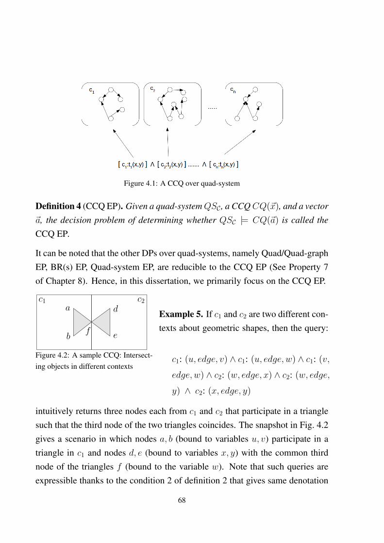
Figure 4.1: A CCQ over quad-system

Definition 4 (CCQ EP). Given a quad-systemQSC , a CCQCQ(~x), and a vector

~a, the decision problem of determining whether QSC |= CQ(~a) is called the

CCQ EP.

It can be noted that the other DPs over quad-systems, namely Quad/Quad-graphEP, BR(s) EP, Quad-system EP, are reducible to the CCQ EP (See Property 7of Chapter 8). Hence, in this dissertation, we primarily focus on the CCQ EP.

a

b

d

e

c1 c2

f

Figure 4.2: A sample CCQ: Intersect-ing objects in different contexts

Example 5. If c1 and c2 are two different con-texts about geometric shapes, then the query:

c1: (u, edge, v) ∧ c1: (u, edge, w) ∧ c1: (v,

edge, w) ∧ c2: (w, edge, x) ∧ c2: (w, edge,

y) ∧ c2: (x, edge, y)

intuitively returns three nodes each from c1 and c2 that participate in a trianglesuch that the third node of the two triangles coincides. The snapshot in Fig. 4.2gives a scenario in which nodes a, b (bound to variables u, v) participate in atriangle in c1 and nodes d, e (bound to variables x, y) with the common thirdnode of the triangles f (bound to the variable w). Note that such queries areexpressible thanks to the condition 2 of definition 2 that gives same denotation

68

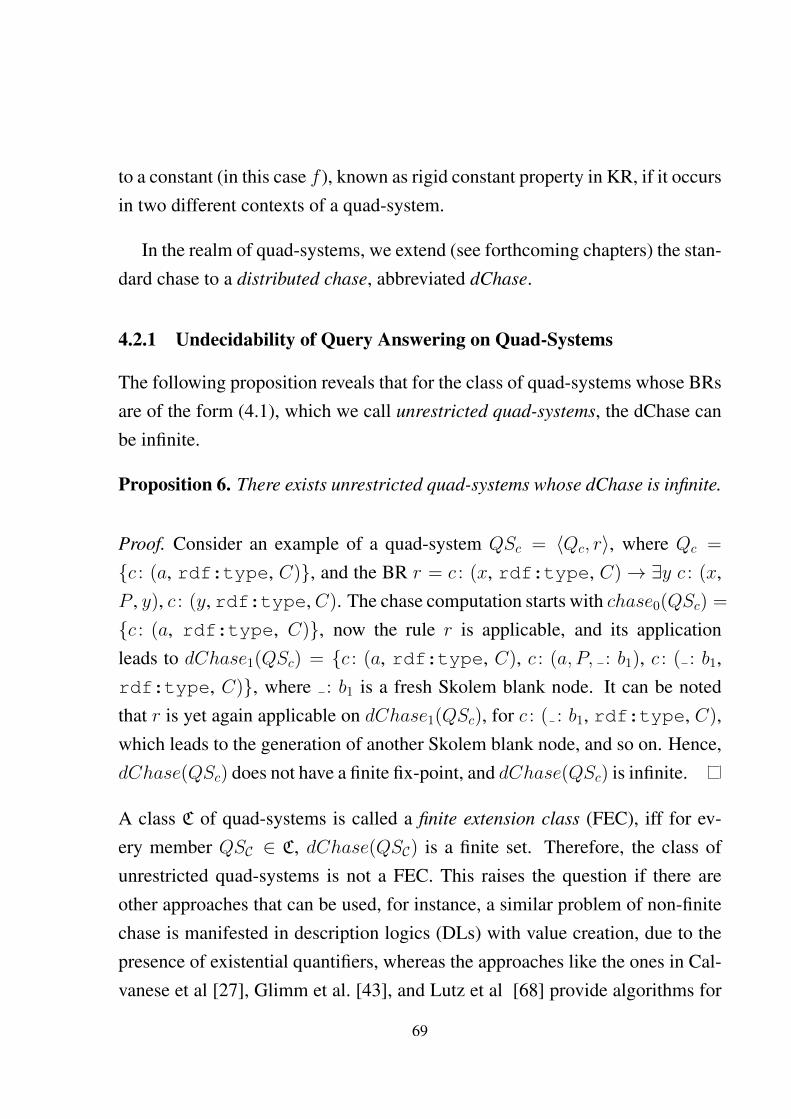
to a constant (in this case f ), known as rigid constant property in KR, if it occursin two different contexts of a quad-system.

In the realm of quad-systems, we extend (see forthcoming chapters) the stan-dard chase to a distributed chase, abbreviated dChase.

4.2.1 Undecidability of Query Answering on Quad-Systems

The following proposition reveals that for the class of quad-systems whose BRsare of the form (4.1), which we call unrestricted quad-systems, the dChase canbe infinite.

Proposition 6. There exists unrestricted quad-systems whose dChase is infinite.

Proof. Consider an example of a quad-system QSc = 〈Qc, r〉, where Qc =

{c : (a, rdf:type, C)}, and the BR r = c : (x, rdf:type, C)→ ∃y c : (x,P , y), c : (y, rdf:type,C). The chase computation starts with chase0(QSc) =

{c : (a, rdf:type, C)}, now the rule r is applicable, and its applicationleads to dChase1(QSc) = {c : (a, rdf:type, C), c : (a, P, : b1), c : ( : b1,rdf:type, C)}, where : b1 is a fresh Skolem blank node. It can be notedthat r is yet again applicable on dChase1(QSc), for c : ( : b1, rdf:type, C),which leads to the generation of another Skolem blank node, and so on. Hence,dChase(QSc) does not have a finite fix-point, and dChase(QSc) is infinite.

A class C of quad-systems is called a finite extension class (FEC), iff for ev-ery member QSC ∈ C, dChase(QSC) is a finite set. Therefore, the class ofunrestricted quad-systems is not a FEC. This raises the question if there areother approaches that can be used, for instance, a similar problem of non-finitechase is manifested in description logics (DLs) with value creation, due to thepresence of existential quantifiers, whereas the approaches like the ones in Cal-vanese et al [27], Glimm et al. [43], and Lutz et al [68] provide algorithms for

69

CQ entailment based on query rewriting. The theorem 7 below establishes thefact that the CCQ EP for unrestricted quad-systems is undecidable.

Theorem 7. The CCQ entailment problem over unrestricted quad-systems is

undecidable.

Proof. (sketch) We show that the well known undecidable problem of non-emptiness of intersection of languages generated by two context-free gram-mars (CFGs) is reducible to the CCQ entailment problem. Given two CFGs,G1 = 〈V1, T, S1, P1〉 and G2 = 〈V2, T, S2, P2〉, where V1, V2, with V1 ∩ V2 =

∅, are the set of variables, T such that T ∩ (V1 ∪ V2) = ∅ is the set of termi-nals. S1 ∈ V1 is the start symbol of G1, and P1 are the set of PRs of the formv → ~w, where v ∈ V , ~w is a sequence of the form w1...wn, where wi ∈ V1 ∪ T .Similarly s2, P2 is defined. Deciding whether the language generated by thegrammars L(G1) and L(G2) have non-empty intersection is known to be unde-cidable [48].

Given two CFGs G1 = 〈V1, T, S1, P1〉 and G2 = 〈V2, T, S2, P2〉, we encodegrammarsG1, G2 into a quad-systemQSc = 〈Qc, R〉, with only a single contextidentifier c. Each PR r = v → ~w ∈ P1 ∪P2, with ~w = w1w2w3..wn, is encodedas a BR of the form: c : (x1, w1, x2), c : (x2, w2, x3), ..., c : (xn, wn, xn+1) →c : (x1, v, xn+1), where x1, .., xn+1 are variables. For each terminal symbol ti ∈T , R contains a BR of the form: c : (x,rdf:type, C) → ∃y c : (x, ti, y),c : (y, rdf:type, C) and Qc is the singleton: { c : (a, rdf:type, C)}. Itcan be proven that:

QSc |= ∃y c : (a, S1, y) ∧ c : (a, S2, y)⇔ L(G1) ∩ L(G2) 6= ∅

We refer the reader to Appendix for the complete proof.

Having shown the undecidability results of query answering of unrestrictedquad-systems, the rest of the thesis focuses on defining subclasses of unre-stricted quad-systems for which query answering is decidable, and establishing

70

their relationships with similar classes in the realm of ∀∃ rules. While definingdecidable classes for quad-systems, one mainly has two fundamentally distinctoptions: (i) is to define notions that solely use the structure/properties of the BRpart, ignoring the quad-graph part, or (ii) to define notions that take into accountboth the BR and quad-graph part. The decidability notions which we define inChapter 6, namely safety, msafety, and csafety belong to type (ii), as these tech-niques takes into account the property of the dChase of a quad-system, whichis determined by both the quad-graph and BRs of the quad-system. Whereasthe ones which we define in chapters 5, 7, namely context acyclic, RR, and re-stricted RR quad-systems fall into type (i), as the properties of BRs alone areused. With an analogy between a set of BRs and a set of ∀∃ rules, and be-tween a quad-graph and a set of ∀∃ instances, the reader should note that suchdistinctions can also been made for the decidability notions realm of ∀∃ rulesets. Techniques such as Weak acyclicity [39], Joint acyclicity [60], and Acyclicgraph of rule dependencies [6] belong to type (ii), as these notions ignore theinstance part. Whereas techniques such as model faithful acyclicity [32] andmodel summarizing acyclicity [32] are of type (i) as both the rules and instancepart is considered.

71

Chapter 5

Context Acyclic Quad-Systems:Decidability via Acyclicity

In the previous chapter, we saw that dChase of unrestricted quad-systems isinfinite and query answering is undecidable, in general. In this chapter, we de-fine a class of quad-systems for which query entailment is decidable. The classis also recognizable [7, 66], i.e. there exists an algorithm that decides for agiven a quad-system whether the quad-system is a member of the class or not.The class has the property that dChase is finite for any member of the class, andhence algorithms based on forward chaining, for deciding query entailment, canstraightforwardly be implemented. It should be noted that the technique we pro-pose is reminiscent of the Weak acyclicity [39, 34] technique used in the realmof Datalog+-. Before we give the description of our class, we first adapt andreformulate the Skolem variant of the chase given in Marnette [69] and CuencaGrau et al [32] to the quad-system settings. We call the reformulated Skolemversion as the Skolem dChase (abbreviated SdChase). The reader should notethat the sources of this chapter has been taken from conference papers [57] and[58].

For any BR r of the form (4.1), the skolemization sk(r) is the result of re-placing each yi ∈ {~y} with a globally unique Skolem function f ri , s.t. f ri : C‖~x‖

→ Bsk. Intuitively, for every distinct vector ~a of constants, with ‖~a‖ = ‖~x‖,

73

f ri (~a) is a fresh blank node, whose node id is a hash of ~a. Let ~f r = 〈f r1 , ..., f r‖~y‖〉be a vector of distinct Skolem functions; for any BR r the form (4.1), with slightabuse we write its skolemization sk(r) as follows:

c1 : t1(~x, ~z), ..., cn : tn(~x, ~z)→ c′1 : t′1(~x,~f r), ..., c′m : t′m(~x, ~f r) (5.1)

Moreover, a skolemized BR r of the form (5.1) can be replaced by the followingequivalent set of formulas, whose symbol size is worst case quadratic w.r.t ‖r‖:

{c1 : t1(~x, ~z), ..., cn : tn(~x, ~z)→ c′1 : t′1(~x,~f r), (5.2)

...,

c1 : t1(~x, ~z), ..., cn : tn(~x, ~z)→ c′m : t′m(~x, ~f r)}

Note that each BR in the above set has exactly one quad pattern with optionalfunction symbols in the head. Also note that a BR without function symbols canbe replaced with a set of BRs with single quad-pattern heads. Hence, w.l.o.g,we assume that any BR in a skolemized set sk(R) of BRs is of the form (5.2).For any quad-graphQC and a skolemized BR r of the form (5.2), the application

of r on QC , denoted by r(QC), is given as:

r(QC) =⋃

µ∈V→C

{c′1 : t′1(~x,

~f r)[µ] | c1 : t1(~x, ~z)[µ] ∈ QC, ..., cn : tn(~x, ~z)[µ]

∈ QC

}For any set of skolemized BRsR, the application ofR onQC is given by: R(QC)

=⋃r∈R r(QC). For any quad-graph QC , we define:

lclosure(QC) =⋃c∈C

{c : (s, p, o) |(s, p, o) ∈ lclosure(graphQC(c))}

For any quad-system QSC = 〈QC, R〉, generating BRs RF is the set of BRsin sk(R) with function symbols, and the non-generating BRs is the set RI =

sk(R) \RF .Let SdChase0(QSC) = lclosure(QC); for i ∈ N, SdChasei+1(QSC) =

lclosure(SdChasei(QSC) ∪RI(SdChasei(QSC))), if RI(SdChasei(QSC))

6⊆ dChasei(QSC);

lclosure(SdChasei(QSC) ∪RF (SdChasei(QSC))), otherwise;

74

The Skolem dChase of QSC , denoted SdChase(QSC), is given as:

SdChase(QSC) =⋃i∈N

SdChasei(QSC)

Intuitively, SdChasei(QSC) can be thought of as the state of SdChase(QSC) atthe end of iteration i. It can be noted that, if there exists i s.t. SdChasei(QSC)= SdChasei+1(QSC), then SdChase(QSC) = SdChasei(QSC). An iterationi, s.t. SdChasei(QSC) is computed by the application of the set of (resp.non-)generating BRs RF (resp. RI) on SdChasei−1(QSC) is called a (resp.non-)generating iteration. A model IC of a quad-system QSC is called univer-

sal [35], iff the following holds: IC is a model of QSC , and for any model I ′C

there exists a homomorphism from IC to I ′C .

Theorem 1. For any consistent quad-system QSC , the following holds: (i)

SdChase(QSC) is a universal model of QSC .1, and (ii) for any boolean CCQ

CQ(),QSC |= CQ() iff there exists a map µ : V(CQ)→ C such that {CQ()}[µ]

⊆ SdChase(QSC).

An analog of the above theorem for DLs and Databases is stated and provedin [27]. Since the proof in [27] can easily be adapted to our case, we re-fer the reader to [27] for the proof. We call the sequence SdChase0(QSC),SdChase1(QSC), ..., the Skolem dChase sequence ofQSC . The following lemmashows that in a dChase sequence of a quad-system, the result of a single gen-erating iteration and a subsequent number of non-generating iterations causesonly an exponential blow up in size.

Lemma 2. For a quad-system QSC = 〈QC, R〉, the following holds: (i) if i ∈ Nis a generating iteration, then ‖SdChasei(QSC)‖ = O(‖SdChasei−1(QSC

)‖‖R‖), (ii) suppose i ∈ N is a generating iteration, and for any j ≥ 1,1Though SdChase(QSC) is not an interpretation in a strict model theoretic sense, one can easily create the

corresponding interpretation ISdChase(QSC) = {Ic = 〈∆c, .c〉}c∈C , s.t. for every c ∈ C, ∆c is equal to set ofconstants in graphSdChase(QSC)(c), and .c is s.t (s, p, o) ∈ graphSdChase(QSC)(c) iff (sc, oc) ∈ pc.

75

i + 1, ..., i + j are non-generating iterations, then ‖SdChasei+j(QSC)‖ =

O(‖SdChasei−1(QSC)‖‖R‖), (iii) for any iteration k, SdChasek(QSC) can be

computed in time O(‖SdChasek−1(QSC)‖‖R‖).

Proof. (Sketch) (i) R can be applied on SdChasei−1(QSC) by grounding R tothe set of constants in SdChasei−1(QSC), the number of such groundings is ofthe order O(‖SdChasei−1(QSC)‖‖R‖), ‖R(SdChasei−1(QSC))‖ = O(‖R‖ ∗‖SdChasei−1(QSC)‖‖R‖). Since lclosure only increases the size polynomially,‖SdChasei(QSC)‖ = O( ‖SdChasei−1( QSC)‖‖R‖).

(ii) From (i) we know that ‖R(SdChasei−1(QSC))‖=O(‖SdChasei−1(QSC

)‖‖R‖). Since, no new constant is introduced in any subsequent non-generatingiterations, and since any quad contains only four constants, the set of constantsin any subsequent dChase iteration is O(4 ∗ ‖SdChasei−1(QSC)‖‖R‖). Sinceonly these many constants can appear in positions c, s, p, o of any quad gen-erated in the subsequent iterations, the size of SdChasei+j(QSC) can only in-crease polynomially, which means that ‖SdChasei+j(QSC)‖ = O(‖SdCha-sei−1(QSC)‖‖R‖).

(iii) Since any dChase iteration k involves the following two operations:(a) lclosure(), and (b) computing R(SdChasek−1(QSC)). (a) can be done inPTIME w.r.t to its input. (b) can be done in the following manner: groundR to the set of constants in SdChasek−1(QSC); then for each grounding g,if body(g) ⊆ SdChasek−1(QSC), then add head(g) to R(SdChasek−1(QSC)).Since, the number of such groundings is of the orderO(‖SdChasek−1(QSC)‖‖R‖),and checking if each grounding is contained in SdChasek−1(QSC), can bedone in time polynomial in ‖SdChasek−1(QSC)‖, the time taken for (b) isO(‖SdChasek−1(QSC)‖‖R‖). Consequently, any iteration k can be done in timeO(‖SdChasek−1(QSC)‖‖R‖).

76

c1: t1(~x, ~z), c2: t2(~x, ~z)→ ∃~y c3: t3(~x, ~y), c4: t4(~x, ~y)

c1

c2

c3

c4

Figure 5.1: Bridge rule: A mechanism for specifying propagation of knowledge between con-texts.

5.1 Context Acyclic Quad-Systems: A Decidable Class

Before we actually introduce our subclass of unrestricted quad-systems, we in-troduce some necessary notations. Consider a BR r of the form: c1 : t1(~x, ~z),c2 : t2(~x, ~z)→ ∃~y c3 : t3(~x, ~y), c4 : t4(~x, ~y). Since such a rule triggers propaga-tion of knowledge in a quad-system, specifically triples from the source contextsc1, c2 to the target contexts c3, c4 in a quad-system. As shown in Fig. 5.1, wecan view a BR as a propagation rule across distinct compartments of knowl-edge, divided as contexts. For any BR of the form (4.1), each context in theset {c′1, ..., c′m} is said to depend on the set of contexts {c1, ..., cn}. In a quad-system QSC = 〈QC, R〉, for any r ∈ R, of the form (4.1), any context whoseidentifier is in the set {c | c : (s, p, o) ∈ head(r), s or p or o is an existentiallyquantified variable}, is called a triple generating context (TGC). One can ana-lyze the set of BRs in a quad-system QSC using a context dependency graph,which is a directed graph, whose nodes are context identifiers in C, s.t. the nodescorresponding to TGCs are marked with a ∗, and whose edges are constructedas follows: for each BR r of the form (4.1), there exists an edge from each cito c′j 6= ci, for each i = 1,. . . , n, j = 1,. . . , m, and for any c ∈ {c1, . . . , cn} ∩{c′1, . . . , c′m} there is an edge from c to c iff there exists c : (s, p, o) ∈ head(r),and s or p or o is an existentially quantified variable. A quad-system is saidto be context acyclic, iff its context dependency graph does not contain cyclesinvolving TGCs.

77

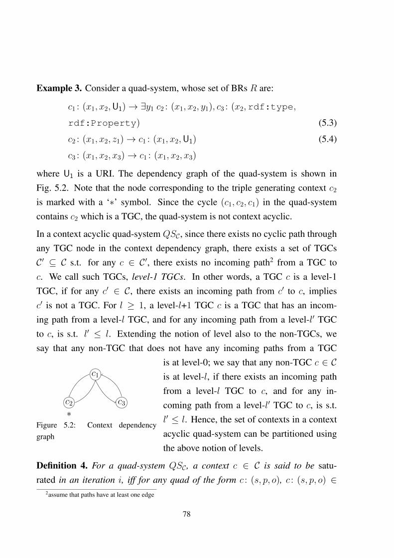
Example 3. Consider a quad-system, whose set of BRs R are:

c1 : (x1, x2,U1)→ ∃y1 c2 : (x1, x2, y1), c3 : (x2,rdf:type,

rdf:Property) (5.3)

c2 : (x1, x2, z1)→ c1 : (x1, x2,U1) (5.4)

c3 : (x1, x2, x3)→ c1 : (x1, x2, x3)

where U1 is a URI. The dependency graph of the quad-system is shown inFig. 5.2. Note that the node corresponding to the triple generating context c2

is marked with a ‘∗’ symbol. Since the cycle (c1, c2, c1) in the quad-systemcontains c2 which is a TGC, the quad-system is not context acyclic.

In a context acyclic quad-system QSC , since there exists no cyclic path throughany TGC node in the context dependency graph, there exists a set of TGCsC ′ ⊆ C s.t. for any c ∈ C ′, there exists no incoming path2 from a TGC toc. We call such TGCs, level-1 TGCs. In other words, a TGC c is a level-1TGC, if for any c′ ∈ C, there exists an incoming path from c′ to c, impliesc′ is not a TGC. For l ≥ 1, a level-l+1 TGC c is a TGC that has an incom-ing path from a level-l TGC, and for any incoming path from a level-l′ TGCto c, is s.t. l′ ≤ l. Extending the notion of level also to the non-TGCs, wesay that any non-TGC that does not have any incoming paths from a TGC

c1

c2

∗c3

Figure 5.2: Context dependencygraph

is at level-0; we say that any non-TGC c ∈ Cis at level-l, if there exists an incoming pathfrom a level-l TGC to c, and for any in-coming path from a level-l′ TGC to c, is s.t.l′ ≤ l. Hence, the set of contexts in a contextacyclic quad-system can be partitioned usingthe above notion of levels.

Definition 4. For a quad-system QSC , a context c ∈ C is said to be satu-rated in an iteration i, iff for any quad of the form c : (s, p, o), c : (s, p, o) ∈

2assume that paths have at least one edge

78

SdChase(QSC) implies c : (s, p, o) ∈ SdChasei(QSC).

Intuitively, context c is saturated in the SdChase iteration i, if no new quadof the form c : (s, p, o) will be generated in any SdChasek(QSC), for any k > i.

5.2 Context Acyclic Quad-Systems: Computational Proper-ties

In this section, we describe some essential computational properties of quad-system class we defined in the previous section. The following lemma gives therelation between the saturation of a context and the required number of SdChaseiterations, for a context acyclic quad-system.

Lemma 5. For any context acyclic quad-system, the following holds: (i) any

level-0 context is saturated before the first generating iteration, (ii) any level-1

TGC is saturated after the first generating iteration, (iii) any level-k context is

saturated before the k + 1th generating iteration.

Proof. Let QSC = 〈QC, R〉 be the quad-system, whose first generating iterationis i.

(i) for any level-0 context c, any BR r ∈ R, and any quad-pattern of the formc : (s, p, o), if c : (s, p, o) ∈ head(r), then for any c′ s.t. c′ : (s′, p′, o′) occurs inbody(r) implies that c′ is a level-0 context and r is a non-generating BR. Also,since c′ is a level-0 context, the same applies to c′. Hence, it turns out that onlynon-generating BRs can bring triples to any level-0 context. Since at the end ofiteration i−1, SdChasei−1(QSC) is closed w.r.t. the set of non-generating BRs(otherwise, by construction of SdChase, i would not be a generating iteration).This implies that c is saturated before the first generating iteration i.

(ii) for any level-1 TGC c, any BR r ∈ R, and any quad-pattern c : (s, p, o),if c : (s, p, o) ∈ head(r), then for any c′ s.t. c′ : (s′, p′, o′) occurs in body(r)

implies that c′ is a level-0 context (Otherwise level of c would be greater than

79

1). This means that only contexts from which triples get propagated to c arelevel-0 contexts. From (i) we know that all the level-0 contexts are saturatedbefore ith iteration, and since during the ith iteration RF is applied followed bythe lclosure() operation (RI need not be applied, since SdChasei−1(QSC) isclosed w.r.t. RI), c is saturated after iteration i, the 1st generating iteration.

(iii) can be obtained from generalization of (i) and (ii), and from the fact thatany level-k context can only have incoming paths from contexts whose levelsare less than or equal to k.

c1

∗

c4

c2

c3

∗

....

..

(a)

c1

∗

c4

c2

c3

∗

....

..

(b)

Figure 5.3: Saturation of contexts

Example 6. Consider the dependency graph in Fig. 5.3a, where .. indicates partof the graph that is not under the scope of our discussion. The TGCs nodes c1

and c3 are marked with a ∗. It can be seen that both c2 and c4 are level-0 contexts,since they do not have any incoming paths from TGCs. Since the only incomingpaths to context c1 are from c2 and c4, which are not TGCs, c1 is a level-1 TGC.Context c3 is a level-2 TGC, since it has an incoming path from the level-1 TGCc1, and has no incoming path from a TGC whose level is greater than 1. Sincethe level-0 contexts only have incoming paths from level-0 contexts and onlyappear on the head part of non-generating BRs, before first generating iteration,

80

all the level-0 TGCs becomes saturated, as the set of non-generating BRs RI

has been exhaustively applied. This situation is reflected in Fig. 5.3b, wherethe saturated nodes are shaded with gray. Note that after the first and secondgenerating iterations c1 and c3 also become saturated, respectively.

The following lemma shows that for context acyclic quad-systems, there ex-ists a finite bound on the size and computation time of its SdChase.

Lemma 7. For any context acyclic quad-system QSC = 〈QC, R〉, the following

holds: (i) the number of SdChase iterations is finite, (ii) size of the SdChase

‖SdChase(QSC)‖ = O(22‖QSC‖), (iii) computing SdChase(QSC) is in 2EXP-TIME, (iv) ifR and the set of schema triples inQC is fixed, then ‖SdChase(QSC)‖is a polynomial in ‖QSC‖, and computing SdChase(QSC) is in PTIME.

Proof. (i) Since QSC is context-acyclic, all the contexts can be partitioned ac-cording to their levels. Also, the number of levels k is s.t. k ≤ |C|. Hence,applying Lemma 2, before the k + 1th generating iteration all the contexts be-comes saturated, and k+1th generating iteration do not produce any new quads,terminating the SdChase computation process.

(ii) In the SdChase computation process, since by Lemma 2, any gener-ating iteration and a sequence of non-generating iterations can only increasethe SdChase size exponentially in ‖R‖, the size of the SdChase before k + 1

th generating iteration is O(‖dChase0(QSC)‖‖R‖k

), which can be written asO(‖QSC‖‖R‖

k

) (†). As seen in (i), there can only be |C| generating iterations,and a sequence of non-generating iterations. Hence, applying k = |C| to (†),and taking into account the fact that |C| ≤ ‖QSC‖, the size of the SdChase‖SdChase(QSC)‖ = O(22‖QSC‖).

(iii) Since in any SdChase iteration except the final one, at least one new quadshould be produced and the final SdChase can have at most O(22‖QSC‖) quads(by ii), the total number of iterations are bounded by O(22‖QSC‖) (†). Sincefrom Lemma 2, we know that for any iteration i, computing SdChasei(QSC) is

81

of the order O(‖SdChasei−1(QSC )‖‖R‖). Since, ‖SdChasei−1(QSC)‖ can atmost beO(22‖QSC‖), computing SdChasei( QSC) is of the orderO(2‖R‖∗2

‖QSC‖).Also since ‖R‖ ≤ ‖QSC‖, any iteration requires O(22‖QSC‖) time (‡). From (†)and (‡), we can conclude that the time required for computing SdChase is in2EXPTIME.

(iv) In (ii) we saw that the size of the SdChase before k+1th generating iter-ation is given byO(‖QSC‖‖R‖

k

) (�). Since by hypothesis ‖R‖ is a constant andalso the size of the dependency graph and the levels in it. Hence, the expression‖R‖k in (�) amounts to a constant z. Hence, ‖SdChase(QSC)‖=O(‖QSC‖z).Hence, the size of SdChase(QSC) is a polynomial in ‖QSC‖.

Also, since in any SdChase iteration except the final one, at least one quadshould be produced and the final SdChase can have at most O(‖QSC‖z) quads,the total number of iterations are bounded by O(‖QSC‖z) (†). Also fromLemma 2, we know that any SdChase iteration i, computing SdChasei(QSC)involves two steps: (a) computing R(SdChasei−1(QSC)), and (b) computinglclosure(), which can be done in PTIME in the size of its input. Since comput-ing R(SdChasei−1(QSC)) is of the order O(‖SdChasei−1(QSC)‖‖R‖), where|R| is a constant and ‖SdChasei−1(QSC)‖ is a polynomial is ‖QSC‖, each iter-ation can be done in time polynomial in ‖QSC‖ (‡). From (†) and (‡), it can beconcluded that SdChase can be computed in PTIME.

Lemma 8. For any context acyclic quad-system, the following holds: (i) data

complexity of CCQ entailment is in PTIME (ii) combined complexity of CCQ

entailment is in 2EXPTIME.

Proof. For a context acyclic quad-systemQSC = 〈QC, R〉, since SdChase(QSC)is finite, a boolean CCQ CQ() can naively be evaluated by grounding the setof constants in the chase to the variables in the CQ(), and then checking ifany of these groundings are contained in SdChase(QSC). The number of suchgroundings can at most be ‖SdChase(QSC)‖‖CQ()‖ (†).

82

(i) Since for data complexity, the size of the BRs ‖R‖, the set of schematriples, and ‖CQ()‖ is fixed to constant. From Lemma 7 (iv), we know thatunder the above mentioned settings the SdChase can be computed in PTIMEand is polynomial in the size of QSC . Since ‖CQ()‖ is fixed to a constant, andfrom (†), binding the set of constants in SdChase(QSC) on CQ() still givesa number of bindings that is worst case polynomial in the size of QSC . Sincemembership of these bindings can checked in the polynomially sized SdChasein PTIME, the time required for CCQ evaluation is in PTIME.

(ii) Since in this case ‖SdChase(QSC)‖ = O(22‖QSC‖) (‡), from (†) and (‡),binding the set of constants in SdChase(QSC) to variables in CQ() amountsto O(2‖CQ()‖∗2‖QSC‖) bindings. Since the size of SdChase is double exponentialin ‖QSC‖, checking the membership of each of these bindings can be done in2EXPTIME. Hence, the combined complexity is in 2EXPTIME.

Theorem 9. For any context acyclic quad-system, the following holds: (i) The

data complexity of CCQ entailment is PTIME-complete, (ii) The combined

complexity of CCQ entailment is 2EXPTIME-complete.

Proof. (i) (Membership) See Lemma 8 for the membership in PTIME.

(Hardness) Follows from the PTIME-hardness of data complexity of CCQentailment for Range Restricted quad-systems (Theorem 3 of Chapter 7), whichare contained in context acyclic quad-systems.

(ii) (Membership) See Lemma 8.

(Hardness) See the following heading.

2EXPTIME-Hardness of CCQ Entailment

In this subsection, we show that the combined complexity of the CCQ EP forcontext acyclic quad-systems is 2EXPTIME-hard. We show this by reductionof the word-problem of a 2EXPTIME deterministic turing machine (DTM) tothe CCQ EP. A DTM M is a tuple M = 〈Q,Σ,∆, q0, qA〉, where

83

• Q is a set of states,

• Σ is a finite alphabet that includes the blank symbol �,

• ∆: (Q× Σ)→ (Q× Σ× {+1,−1}) is the transition function,

• q0 ∈ Q is the initial state.

• qA ∈ Q is the accepting state.

W.l.o.g. we assume that there exists exactly one accepting state, which is alsoa halting state. A configuration is a word ~α ∈ Σ∗QΣ∗. A configuration ~α2 is asuccessor of the configuration ~α1, iff one of the following holds:

1. ~α1 = ~wlqσσr ~wr and ~α2 = ~wlσ′q′σr ~wr, if ∆(q, σ) = (q′, σ′, R), or

2. ~α1 = ~wlqσ and ~α2 = ~wlσ′q′�, if ∆(q, σ) = (q′, σ′, R), or

3. ~α1 = ~wlσlqσ ~wr and ~α2 = ~wlq′σlσ

′ ~wr, if ∆(q, σ) = (q′, σ′, L).

where q, q′ ∈ Q, σ, σ′, σl, σr ∈ Σ, and ~wl, ~wr ∈ Σ∗. Since number of con-figurations can at most be doubly exponential in the size of the input string,the number of tape cells traversed by the DTM tape head is also bounded dou-ble exponentially. A configuration ~c = ~wlq ~wr is an accepting configuration iffq = qA. A language L ⊆ Σ∗ is accepted by a 2EXPTIME bounded DTM M ,iff for every ~w ∈ L, M accepts ~w in time O(22‖~w‖

).

Simulating DTMs using Context Acyclic Quad-Systems

Consider a DTM M = 〈Q,Σ,∆, q0, qA〉, and a string ~w, with ‖~w‖ = m.Suppose that M terminates in 22n time, where n = mk, k is a constant. Inorder to simulate M , we construct a quad-system QSMC = 〈QM

C , R〉, whereC = {c0, c1, ..., cn}, whose various elements represents the constructs ofM . Wefollow the technique in works such as [23, 60] to iteratively generate a doubly

84

exponential number of objects that represent the cells of the tape of the DTM.Let QM

C be initialized with the following quads:

c0 : (k0,rdf:type, R), c0 : (k1,rdf:type, R),

c0 : (k0,rdf:type,min0), c0 : (k1,rdf:type,max0), c0 : (k0, succ0, k1)

Now for each pair of elements of typeR in ci, a Skolem blank-node is generatedin ci+1, and hence follows the recurrence relation r(m+1) = [r(m)]2, with seedr(0) = 2, which after n iterations yields 22n. In this way, a doubly exponentiallylong chain of elements is created in cn using the following set of rules:

ci : (x0,rdf:type, R), ci : (x1,rdf:type, R)→

∃y ci+1 : (x0, x1, y), ci+1 : (y,rdf:type, R)

The combination of the minimal element with the minimal element (elementsof type mini) in ci create the minimal element in ci+1, and similarly the com-bination of the maximal element with the maximal element (elements of typemaxi) in ci create the maximal element of ci+1:

ci+1 : (x0, x0, x1), ci : (x0,rdf:type,mini)→ ci+1 : (x1,rdf:type,mini+1)

ci+1 : (x0, x0, x1), ci : (x0,rdf:type,maxi)→ ci+1 : (x1,rdf:type,maxi+1)

The successor relation succi+1 is created in ci+1 using the following set of rules,using the well-known integer counting technique:

ci : (x1, succi, x2), ci+1 : (x0, x1, x3), ci+1 : (x0, x2, x4)→ ci+1 : (x3, succi+1, x4)

ci : (x1, succi, x2), ci+1 : (x1, x3, x5), ci+1 : (x2, x4, x6), ci : (x3,rdf:type,

maxi), ci : (x4,rdf:type,mini)→ ci+1 : (x5, succi+1, x6)

Each of the above set of rules are instantiated for 0 ≤ i < n, and in this wayafter n generating SdChase iterations, cn has doubly exponential number of

85

elements of type R, that are ordered linearly using the relation succn. By virtueof the first rule below, each of the objects representing the cells of the DTMare linearly ordered by the relation succ. Also the transitive closure of succ isdefined as the relation succt

cn : (x0, succn, x1)→ cn : (x0, succ, x1)

cn : (x0, succ, x1)→ cn : (x0, succt, x1)

cn : (x0, succt, x1), cn : (x1, succt, x2)→ cn : (x0, succt, x2)

Also using a similar construction, we can create a linearly ordered chain of adoubly exponential number of objects in cn that represents configurations ofM ,whose minimal element is of type conInit, and the linear order relation beingconSucc.

Various triple patterns that are used to encode the possible configurations,runs, and their relations in M are:

(x0, head, x1) denotes the fact that in configuration x0, the head of the DTM isat cell x1.

(x0, state, x1) denotes the fact that in configuration x0, the DTM is in state x1.

(x0, σ, x1) where σ ∈ Σ, denotes the fact that in configuration x0, the cell x1

contains σ.

(x0, succ, x1) denotes the linear order between cells of the tape.

(x0, succt, x1) denotes the transitive closure of succ.

(x0, conSucc, x1) to denote the fact that x1 is a successor configuration of x0.

(x0,rdf:type, Accept) denotes the fact that the configuration x0 is an ac-cepting configuration.

86

Since in our construction, each σ ∈ Σ is represented as a relation, we could con-strain that no two alphabets σ 6= σ′ are on the same cell in a given configurationusing the following axiom:

cn : (z1, σ, z2), cn : (z1, σ′, z2)→

for each σ 6= σ′ ∈ Σ. Note that the above BR has an empty head, is equivalentto asserting the negation of its body.

Initialization Suppose the initial configuration is q0 ~w�, where ~w = σ0...σn−1.We encode this in our quad-system QSMC using the following BRs:

cn : (x0,rdf:type, conInit), cn : (x1,rdf:type,minn)→ cn : (x0, head,

x1), cn : (x0, state, q0)

cn : (x0,rdf:type,minn) ∧n−1∧i=0

cn : (xi, succ, xi+1) ∧ cn : (xj,rdf:type,

conInit)→n−1∧i=0

cn : (xj, σi, xi) ∧ cn : (xj,�, xn)

cn : (xj,rdf:type, conInit), cn : (xj,�, x0), cn : (x0, succt, x1)→ cn : (xj,

�, x1)

The last BR copies the � to every succeeding cell in the initial configuration.

Transitions For every left transition ∆(q, σ) = (qj, σ′,−1), the following BR:

cn : (x0, head, xi), cn : (x0, σ, xi), cn : (x0, state, q), cn : (xj, succ, xi), cn : (x0,

conSucc, x1)→ cn : (x1, head, xj), cn : (x1, σ′, xi), cn : (x1, state, qj)

For every right transition ∆(q, σ) = (qj, σ′,+1), the following BR:

cn : (x0, head, xi), cn : (x0, σ, xi), cn : (x0, state, q), cn : (xi, succ, xj), cn : (x0,

conSucc, x1)→ cn : (x1, head, xj), cn : (x1, σ′, xi), cn : (x1, state, qj)

87

Inertia If in any configuration the head is at cell i of the tape, then in everysuccessor configuration, elements in preceding and following cells of i in thetape are retained. The following two BRs ensures this:

cn : (x0, head, xi), cn : (x0, conSucc, x1), cn : (xj, succt, xi), cn : (x0, σ, xj)

→ cn : (x1, σ, xj)

cn : (x0, head, xi), cn : (x0, conSucc, x1), cn : (xi, succt, xj), cn : (x0, σ, xj)

→ cn : (x1, σ, xj)

The rules above are instantiated for every σ ∈ Σ.

Acceptance Any configuration whose state is qA is accepting:

cn : (x0, state, qA)→ cn : (x0,rdf:type, Accept)

If a configuration of accepting type is reached, then it can be back propagatedto the initial configuration, using the following BR:

cn : (x0, conSucc, x1), cn : (x1,rdf:type, Accept)→ cn : (x0,rdf:type,

Accept)

Finally M accepts ~w iff the initial configuration is an accepting configuration.Let CQM be the CCQ: ∃y cn : (y, rdf:type, conInit), cn : (y, rdf:type,Accept). It can easily be verified thatQSMC |= CQM iff the initial configurationis an accepting configuration. In order to prove the soundness and completenessof our simulation, we prove the following claims:

Claim (1) The quad-systemQSMC in the aforementioned simulation is a contextacyclic quad-system

Since there is no edge from any cj to ci, for each 1 ≤ i < j ≤ n, the contextdependency graph for QSMC is acyclic, and hence QSMC is context acyclic.

Claim (2) QSMC |= CQM iff M accepts ~w.

88

Suppose that QSMC |= CQM , then by Theorem 1, there exists an assignmentµ : V(CQM) → C, with CQM [µ] ⊆ dChase(QSC). This implies that thereexists a constant o in C(SdChase(QSC)), with {cn : (o, rdf:type, Accept),cn : (o, rdf:type, conInit)} ⊆ SdChase(QSC . But thanks to the acceptanceaxioms it follows that there exists an constant o′ such that {cn : (o, conSucc,o1), cn : (o1, conSucc, o2), . . . , cn : (on, conSucc, o′)} ⊆ SdChase(QSC), andcn : (o′, rdf:type, Accept) ∈ SdChase(QSC). Also thanks to the initializa-tion axioms, it can be seen that o represents the initial configuration of M i.e.it represents the configuration in which the initial state is q0, and the left end ofthe read-write tape contains ~w followed by trailing �s, with the read-write headpositioned at the first cell of the tape. Also the transition axioms makes sure thatif cn : (o, conSucc, o′′) ∈ SdChase(QSC), then o′′ represents a successor con-figuration of o. That is, if o represents the configuration in which M is at stateq with read-write head at position pos of the tape that contains a letter σ ∈ Σ,and if ∆(q, σ) = (q′, σ′, D), then o′′ represents the configuration in which Mis at state q′, in which read-write head is at the position pos − 1/pos + 1 de-pending on whether D = −1/ + 1, and σ′ is at the position pos of the tape. Asa consequence of the above arguments, it follows that o′ represents an accept-ing configuration of M , i.e. a configuration in which the state is qA, the loneaccepting, halting state. This means that M accepts the string ~w.

For the converse, we briefly show that if QSMC 6|= CQM then M does notaccept ~w. Suppose that QSMC 6|= CQM , then by Theorem 1, for every assign-ment µ : V(CQM)→C, it should be the case that CQM [µ] 6⊆ SdChase(QSC).Thanks to the initialization axioms, we know that there exists a constant o ∈C(SdChase(QSC)) with cn : (o, rdf:type, conInit) ∈ SdChase(QSC). Weknow that o represents the initial configuration of M . Also by the initial con-struction axioms ofQSMC , we know that o is the initial element of a double expo-nential chain of objects that are linearly ordered by property symbol conSucc.From transition axioms we know that, if, for any o′′, cn : (o, conSucc, o′′) ∈

89

dChase(QSC), then o′′ represents a valid successor configuration of o, whichitself holds for o′′, and so on. This means that for none of the succeeding doubleexponential configurations of M , the accepting state qA holds. This means thatM does not reach an accepting configuration with string ~w, and hence rejects it.

Since we polynomially reduced the word problem of 2EXPTIME DTM,which is a 2EXPTIME-hard problem, to the CCQ EP over context acyclic quad-systems, it immediately follows that CCQ EP over context acyclic quad-systemsis 2EXPTIME-hard.

Reconsidering the quad-system in example 3, which is not context acyclic.Suppose that the contexts are enabled with RDFS inferencing, i.e lclosure() =

rdfsclosure(). During SdChase construction, since any application of rule (5.3)can only create a triple in c2 in which the Skolem blank node is in the objectposition, where as the application of rule (5.4), does not propagate constantsin object position to c1. Although at a first look, the SdChase might seem toterminate, but since the application of the following RDFS inference rule in c2:(s, p, o) → (o, rdf:type, rdfs:Resource), derives a quad of the formc2 : ( :b, rdf:type, rdfs:Resource), where :b is the Skolem blank-node created by the application of rule (5.3). Now by application of rule (5.4)leads to c1 : ( :b,rdf:type, U1). Since rule (5.3) is applicable on c1 : ( :b,rdf:type, U1), which again brings a new Skolem blank node to c2. Sincethis goes on indefinitely, the SdChase construction does not terminate. Hence,as seen above the notion of context acyclicity can alarm us about such infinitecases.

90

Chapter 6

Csafe, Msafe, and Safe Quad-Systems:Restricting the Descendency Structure ofSkolem Blank-nodes

In the preceding chapter, we introduced context acyclic quad-systems, a classfor which query answering is decidable. To briefly sum up, in context acyclicitytechnique a context dependency graph is used to model the propagation pathof constants across various contexts in the rules, and restricts the dependencygraph to be acyclic. One of the main drawback of context acyclicity is that itonly analyzes the BR part of a quad-system, and ignores the quad-graph part,producing a large number of false alarms. That is it so happens, for large num-ber of cases, that although context dependency graph is cyclic, the dChase isfinite. To compensate this drawback, in this chapter, we define more expressiveclasses of quad-systems, namely SAFE, MSAFE and CSAFE, that are FECs andfor which query entailment is decidable. Finiteness/Decidability is achieved byputting certain restrictions (explained below) on the blank nodes generated inthe dChase. Before we give the description of our class, we first adapt and refor-mulate the restricted variant of the chase given in Fagin et al. [39] (also callednon-oblivious chase) to the quad-system settings.

For a set of quad-patterns S and a set of terms T , we define the relation

91

T -connectedness between quad-patterns in S as the least relation with:

• q1 and q2 are T -connected, if CV(q1) ∩ CV(q2) ∩ T 6= ∅, for any twoquad-patterns q1, q2 ∈ S,

• if q1 and q2 are T -connected, and q2 and q3 are T -connected, then q1 andq3 are also T -connected, for any quad-patterns q1, q2, q3 ∈ S.

It can be noted that T -connectedness is an equivalence relation and partitions Sinto a set of T -components (similar notion is called a piece in Baget et al. [6]).Note that for two distinct T -components P1, P2 of S, CV(P1)∩CV(P2)∩T = ∅.For any BR r = body(r)(~x, ~z)→ head(r)(~x, ~y), suppose P1, P2, . . . , Pk are thepairwise distinct {~y}-components of head(r)(~x, ~y), then r can be replaced bythe semantically equivalent set of BRs {body(r)(~x, ~z)→ P1, . . . , body(r)(~x, ~z)

→ Pk} whose symbol size is worst case quadratic w.r.t. the symbol size of r.Hence, w.l.o.g. we assume that for any BR r, the set of quad-patterns head(r)

is a single component w.r.t. the set of existentially quantified variables in r.

Considering the fact that the local semantics for contexts are fixed a priori(for instance RDFS), both the number of rules in the set of local inference rulesLIR and the size of each rule in LIR can be assumed to be a constant. Note thateach local inference rule is range restricted and does not contain existentiallyquantified variables in its head. Any ir ∈ LIR is of the form:

∀~x∀~z [t1(~x, ~z) ∧ . . . ∧ tk(~x, ~z)→ t′1(~x)], (6.1)

where ti(~x, ~z), for i = 1, . . . , n are triple patterns, whose variables are from{~x} or {~z}, and t′1(~x) is a triple pattern, whose variables are from {~x}. Hence,for any quad-system QSC = 〈QC , R〉 in order to accomplish the effect of localinferencing in each context c ∈ C, for each ir ∈ LIR of the form (6.1), we couldaugment R with a BR irc of the form:

∀~x∀~z [c : t1(~x, ~z) ∧ . . . ∧ c : tk(~x, ~z)→ c : t′1(~x)]

92

Since ‖LIR‖ is a constant and the size of the augmentation is linear in |C|,w.l.o.g we assume that the set R contains a BR irc, for each ir ∈ LIR, c ∈ C.

For any BR r = body(r)(~x, ~z)→ head(r)(~x, ~y) and an assignment µ : {~x}∪ {~z} → C, the application of µ on r is defined as:

apply(r, µ) = head(r)[µext(~y)]

where µext(~y) ⊇ µ s.t. µext(~y)(yi) = : b is a fresh blank node from Bsk, for eachyi ∈ {~y}.

We assume that there exists an order ≺l (for instance, lexicographic order)on the set of constants. We extend ≺l to the set of quads s.t. for any twoquads c : (s, p, o) and c′ : (s′, p′, o′), c : (s, p, o) ≺l c′ : (s′, p′, o′), iff c ≺l c′, orc = c′, s ≺l s′, or c = c′, s = s′, p ≺l p′, or c = c′, s = s′, p = p′, o ≺l o′. It canbe noted that ≺l is a strict linear order over the set of all quads. For any finitequad-graph QC , the≺l-greatest quad of QC , denoted greatestQuad≺l

(QC), is thequad q ∈ QC s.t. q′ ≺l q, for every other q′ ∈ QC . Also, the order ≺q is definedover the set of finite quad-graphs as follows: for any two finite quad-graphs QC ,Q′C′,

QC ≺q Q′C′, if (i) QC ⊂ Q′C′;

QC ≺q Q′C′, if (i) does not hold and (ii) greatestQuad≺l(QC \ Q′C′) ≺l

greatestQuad≺l(Q′C′ \ QC);

QC 6≺q Q′C′, if both (i) and (ii) are not satisfied;

A relation R over a set A is called a strict linear order iff R is irreflexive,transitive, and R(a, b) or R(b, a) holds, for every distinct a, b ∈ A.

Property 1. LetQ be the set of all finite quad-graphs;≺q is a strict linear order

over Q.

Also, we now define in parallel the dChase of a quad-system QSC = 〈QC , R〉and the level of a quad in dChase ofQSC as follows: any quad inQC is of level 0.

93

The level of a set of quads is the largest among levels of quads in the set. Levelof any quad that results from the application of a BR r w.r.t. an assignment µ isone more than the level of the set body(r)[µ], if it has not already been assigneda level. Let ≺ be an ordering on the quad-graphs s.t. for any two quad-graphsQ′C′ and Q′′C′′ of the same level, Q′C′ ≺ Q′′C′′, iff Q′C′ ≺q Q′′C′′. For Q′C′ and Q′′C′′ ofdifferent levels,Q′C′ ≺ Q′′C′′, iff level ofQ′C′ is less than level ofQ′′C′′. It can easilybe seen that ≺ is a strict linear order over the set of quad-graphs. For any BRsr, r′ and assignments µ, µ′ over V(body(r)),V(body(r′)), respectively, (r, µ)≺(r′, µ′) iff body(r)[µ] ≺ body(r′)[µ′]. For any quad-graph Q′C′, a set of BRs R, aBR r ∈ R, an assignment µ ∈ V(body(r)) → C, let applicableR(r, µ,Q′C′) bethe least ternary predicate inductively defined as:

applicableR(r, µ,Q′C′) holds, if (a) body(r)[µ] ⊆ Q′C′, head(r)[µ′′] 6⊆ Q′C′,

∀µ′′ ⊇ µ, and (b) 6 ∃r′ ∈ R, 6 ∃µ′s.t. r′ 6= r or µ′ 6= µ with (r′, µ′) ≺ (r, µ)

and applicableR(r′, µ′, Q′C′);

For any quad-system QSC = 〈QC, R〉, letdChase0(QSC) = QC;dChasei+1(QSC) = dChasei(QSC)∪ apply(r, µ), if there exists r= body(r)(~x,

~z)→ head(r)(~x, ~y) ∈ R, assignment µ : {~x} ∪ {~z} →C s.t. applicableR(r, µ,dChasei(QSC));dChasei+1(QSC) = dChasei(QSC), otherwise; for any i ∈ N. The dChase

of QSC , noted dChase(QSC), is given as:

dChase(QSC) =⋃i∈N

dChasei(QSC)

Intuitively, dChasei(QSC) can be thought of as the state of dChase(QSC) atthe end of iteration i. It can be noted that, if there exists i s.t. dChasei(QSC)= dChasei+1(QSC), then dChase(QSC) = dChasei( QSC). A model IC of aquad-systemQSC is called universal [35], iff the following holds: IC is a modelof QSC , and for any model I ′C there exists a homomorphism from IC to I ′C .

94

Theorem 2. For any consistent quad-system QSC , the following holds: (i)

dChase(QSC) is a universal model of QSC .1, and (ii) for any boolean CCQ

CQ(),QSC |= CQ() iff there exists a map µ : V(CQ)→ C such that {CQ()}[µ]

⊆ dChase(QSC).

We call the sequence dChase0(QSC), dChase1(QSC), ..., the dChase se-

quence of QSC . The following lemma shows that in a dChase sequence of aquad-system, any dChase iteration can be performed in time exponential w.r.tthe size of the largest BR.

Lemma 3. For a quad-system QSC = 〈QC, R〉, for any i ∈ N+, the following

holds: (i) dChasei(QSC) can be computed in time O( |R| ∗ ‖dChasei−1(QSC

)‖rs), where rs = maxr∈R‖r‖, (ii) ‖dChasei(QSC)‖ =O(‖dChasei−1(QSC)‖+ ‖R‖).

Proof. (i) We can first find, if there exists an r ∈ R, assignment µ s.t. applicableR(r, µ, dChasei−1(QSC)) holds, in the following naive way: (1) bind theset of variables in all rules in R with the set of constants in dChasei−1(QSC).Let this set be called S. Note that |S| = O(|R| ∗ ‖dChasei−1(QSC )‖‖rs‖),where rs = maxr∈R‖r‖. Also, note that each of the binding in S is of the formbody(r)(~x, ~z)(µ)→ head(r)(~x, ~y)(µ′) (♥), where r ∈ R. (2) From the set S wefilter out every binding of the form (♥) in which ~x[µ] 6= ~x[µ′]. Let S ′ be the re-sulting set after the above filtering operation. (3) From the set S ′, we now filterout all the bindings of the form (♥) with head(r)(~x, ~y)(µ′)⊆ dChasei−1(QSC),with resulting set S ′′. (4) If S ′′ = ∅, then there no r ∈ R, assignment µs.t. applicableR(r, µ, dChasei−1(QSC)) is True. Otherwise if S ′′ 6= ∅, thennote that each binding of the form (♥) in S ′′ is s.t. condition (a) of the trueapplicableR(r, µ, dChasei−1(QSC)) is satisfied. Now, we can sort S ′′ w.r.t. ≺

1Though dChase(QSC) is not an interpretation in a strict model theoretic sense, one can easily create thecorresponding interpretation IdChase(QSC) = {Ic = 〈∆c, .c〉}c∈C , s.t. for every c ∈ C, ∆c is equal to set ofconstants in graphdChase(QSC)(c), and .c is s.t (s, p, o) ∈ graphdChase(QSC)(c) iff (sc, oc) ∈ pc.

95

and select the least binding b of the form (♥), so that condition (b) in True condi-tion of applicableR() is satisfied for b. It can easily be seen that applicableR(r,µ, dChasei−1(QSC)) holds for the r, µ extracted from b. Since the size ofeach binding is at most rs, the operations (1)-(4) can be performed in timeO(|R| ∗ ‖dChasei−1(QSC)‖rs). Since dChasei(QSC) = dChasei−1(QSC) ∪head(r)[µ], for r, µ with applicableR(r, µ, dChasei−1(QSC)), dChasei(QSC)can be computed in time O(‖dChasei−1(QSC )‖rs).

(ii) Trivially holds, since in the worst case dChasei(QSC) = dChasei−1(QSC)

∪ head(r)[µ], for r ∈ R.

Lemma 4. For any quad-systemQSC , If : b is a Skolem blank node in dChase(QSC),

generated by the application of assignment µ on r= body(r)(~x, ~z)→ head(r)(~x,

~y), with µext(~y)(yj) = : b, yj ∈ {~y}, then : b is unique for (r, yj, ~x[µext(~y)]).

Proof. By contradiction, suppose if : b is not unique for (r, yj, ~x[µext(~y)]), i.e.there exists : b′ 6= : b in dChase(QSC), with : b′ generated by r such that: b′ = µ′ext(~y)(yj) and ~x[µext(~y)] = ~x[µ′ext(~y)]. W.l.o.g. suppose : b was gen-

erated in an iteration l ∈ N and : b′ in an iteration m > l. This means thathead(r)(~x, ~y)[µext(~y)] ⊆ dChasel(QSC), and hence head(r)(~x, ~y)[µext(~y)] ⊆dChasem−1(QSC). Also, since µ|~x = µ′|~x, there ∃µ′′ ⊇ µ′ s.t. head(r)(~x, ~y)[µ′′]

⊆ dChasem−1(QSC). This means that (a) part of the function applicableR isfalse, for applicableR(r, µ′, dChasem−1(QSC)) to be true, and as a consequenceapplicableR(r, µ′, dChasem−1(QSC)) is false. Hence, our assumption that : b′

= yj[µ′ext(~y)] is false. Hence, : b is unique for (r, yj, ~x[µext(~y)]).

6.1 Csafe, Msafe, and Safe Quad-Systems: Decidable Classes

Recall that, for any quad-systemQSC , the set of blank-nodes B(dChase(QSC))

in its dChase(QSC) not only contains blank nodes present inQSC , i.e. B(QSC),but also contains Skolem blank nodes that are generated during the dChase con-struction process. Note that the following relation holds: Bsk(dChase(QSC))

96

= B(dChase(QSC)) \ B(QSC). We assume w.l.o.g. that for any set of BRs R,any BR in R has a unique rule identifier, and we often write ri for the BR in R,whose identifier is i.

Definition 5 (Origin RuleId/Vector). For any Skolem blank node : b, generated

in the dChase by the application of a BR ri = body(ri)(~x, ~z)→ head(ri)(~x, ~y)

using assignment µ : {~x}∪{~z} → C, i.e. : b = µext(~y)(yj), for some yj ∈ ~y, we

say that the origin ruleId of : b is i, denoted originRuleId( : b) = i. Moreover

~w = ~x[µ] is said to be the origin vector of : b, denoted originV ector( : b) =

~w.

As we saw in Lemma 4, any such Skolem blank node : b, generated in thedChase can uniquely be represented by the expression (i, j, ~w), where i is therule id, j is the identifier of the existentially quantified variable yj in ri sub-stituted by : b during the application of µ on ri. Also in the above case, wedenote relation between each constant k = µext(~y)(xh), xh ∈ {~x}, and : b withthe relation childOf. Moreover, since children of a Skolem blank node can beSkolem blank nodes, which themselves can have children, one can naturally de-fine relation descendantOf =childOf+ as the transitive closure of childOf. Notethat according to the above definition, ‘descendantOf’ is not reflexive. In addi-tion, we could keep track of the set of contexts in which a blank-node was firstgenerated, using the following notion:

Definition 6 (Origin-contexts). For any quad-system QSC and for any Skolem

blank node : b ∈Bsk(dChase(QSC)), the set of origin-contexts of : b is given

by originContexts( : b) = {c | ∃i. c:(s, p, o) ∈ dChasei(QSC), s = : b or p

= : b or o = : b, and @j < i with c′:(s′, p′, o′) ∈ dChasej(QSC), s′ = : b or

p′ = : b or o′ = : b, for any c′ ∈ C}.

Intuitively, origin-contexts for a Skolem blank node : b is the set of contexts inwhich triples containing : b are first generated, during the dChase construction.Note that there can be multiple contexts in which : b can simultaneously be

97

generated. By setting originRuleId(k) = n.d., (resp. originV ector(k) =

n.d., resp. originContexts(k) = n.d.,) where n.d. is an ad hoc constant, forevery k 6∈ Bsk(dChase(QSC)), we extend the definition of origin ruleId, (resp.origin vector, resp. origin-contexts) to all the constants in the dChase of a quad-system.

Example 7. Consider the quad-system 〈QC, R〉, where QC = {c1 : (a, b, c)}.Suppose R is the following set:

R =

c1 : (x11, x12, z1)→ c2 : (x11, x12, y1) (r1)

c2 : (a, z2, x22)→ c3 : (a, x22, y2) (r2)

c2 : (z3, b, x32)→ c3 : (b, x32, y3) (r3)

c3 : (a, z41, x41), c3 : (b, z42, x42)

→ c2 : (y4, x41, a), c2 : (y4, x42, b) (r4)

Suppose that for brevity quantifiers have been omitted, and variables of the formyi or yij are implicitly existentially quantified. Iterations during the dChaseconstruction are:

dChase0(QSC) = {c1:(a, b, c)}

dChase1(QSC) = {c1 : (a, b, c), c2 : (a, b, : b1)}

dChase2(QSC) = {c1:(a, b, c), c2 : (a, b, : b1), c3 : (a, : b1, : b2)}

dChase3(QSC) = {c1:(a, b, c), c2 : (a, b, : b1), c3 : (a, : b1, : b2),

c3 : (b, : b1, : b3)}

dChase4(QSC) = {c1:(a, b, c), c2 : (a, b, : b1), c3 : (a, : b1, : b2),

c3 : (b, : b1, : b3), c2 : ( : b4, : b2, a), c2 : ( : b4, : b3, b)}

dChase5(QSC) = dChase4(QSC),

Also note:originRuleId( : b1) = 1, originRuleId( : b2) = 2, originRuleId( : b3) =

3, originRuleId( : b4) = 4,

98

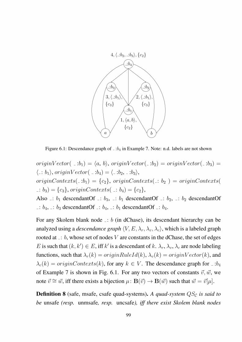
:b4

4, 〈 :b2, :b3〉, {c2}

:b3

3, 〈 :b1〉,{c3}

:b2

2, 〈 :b1〉,{c3}

:b1

1, 〈a, b〉,{c2}

a b

Figure 6.1: Descendance graph of :b4 in Example 7. Note: n.d. labels are not shown

originV ector( :b1) = 〈a, b〉, originV ector( :b2) = originV ector( :b3) =

〈 : b1〉, originV ector( :b4) = 〈 :b2, :b3〉,originContexts( :b1) = {c2}, originContexts( : b2 ) = originContexts(

: b3) = {c3}, originContexts( : b4) = {c2},Also : b1 descendantOf : b3, : b1 descendantOf : b2, : b2 descendantOf: b4, : b3 descendantOf : b4, : b1 descendantOf : b4.

For any Skolem blank node : b (in dChase), its descendant hierarchy can beanalyzed using a descendance graph 〈V,E, λr, λv, λc〉, which is a labeled graphrooted at : b, whose set of nodes V are constants in the dChase, the set of edgesE is such that (k, k′) ∈ E, iff k′ is a descendant of k. λr, λv, λc are node labelingfunctions, such that λr(k) = originRuleId(k), λv(k) = originV ector(k), andλc(k) = originContexts(k), for any k ∈ V . The descendance graph for :b4

of Example 7 is shown in Fig. 6.1. For any two vectors of constants ~v, ~w, wenote ~v ∼= ~w, iff there exists a bijection µ : B(~v)→ B(~w) such that ~w = ~v[µ].

Definition 8 (safe, msafe, csafe quad-systems). A quad-system QSC is said to

be unsafe (resp. unmsafe, resp. uncsafe), iff there exist Skolem blank nodes

99

: b 6= : b′ in dChase(QSC) such that : b is a descendant of : b′, with

originRuleId( : b) = originRuleId( : b′) and originV ector( : b) ∼=originV ector( : b′) (resp. originRuleId( : b) = originRuleId( : b′), resp.

originContexts( : b) = originContexts( : b′)). A quad-system is safe (resp.

msafe, resp. csafe) iff it is not unsafe (resp. unmsafe, resp. uncsafe).

Intuitively, safe, msafe and csafe quad-systems, does not allow repetitive gener-ation of Skolem blank-nodes with a certain set of attributes in its dChase. Thecontainment relation between the class of safe, msafe, and csafe quad-systemsare established by the following theorem:

Theorem 9. Let SAFE,MSAFE, and CSAFE denote the class of safe, msafe, and

csafe quad-systems, respectively, then the following holds:

CSAFE ⊂ MSAFE ⊂ SAFE

Proof. We first show MSAFE ⊆ SAFE, by showing the inverse inclusion of theircompliments, i.e. UNSAFE ⊆ UNMSAFE. Suppose a given quad-system QSC isunsafe, then by definition its dChase contains two distinct Skolem blank nodes: b, : b′ such that : b is a descendant of : b′, with originRuleId( : b) =

originRuleId( : b′) and originV ector( : b)∼= originV ector( : b′). But thisimplies that originRuleId( : b) = originRuleId( : b′). Hence, by definition,QSC is unmsafe. Hence UNSAFE ⊆ UNMSAFE (†).

Now, we show that CSAFE ⊆ MSAFE by showing UNMSAFE ⊆ UNCSAFE.Suppose a given quad-system QSC = 〈QC, R〉 is unmsafe, then by definition itsdChase contains two distinct Skolem blank nodes : b, : b′ such that : b is adescendant of : b′, with originRuleId( : b) = originRuleId( : b′). But thisimplies that there exists a BR ri = body(ri)(~x, ~z)→ head(ri)(~x, ~y), assignmentµ, (resp. µ′,) s.t. : b (resp. : b′) was generated in dChase(QSC) as result ofapplication of µ (resp. µ′) on ri. That is : b= yj[µ

ext(~y)], and : b′ = yk[µ′ext(~y)],

where yj, yk ∈ {~y}. We have the following two subcases (i) j = k, (ii) j 6= k.

100

Suppose (i) j = k, then it immediately follows that originContexts( : b) =

originContexts( : b′). Hence, QSC is uncsafe. Suppose (ii) j 6= k, then byconstruction of dChase, on application of µ′ to ri, along with : b′, there getsalso generated a Skolem blank node : b′′ = yj[µ

′ext(~y)], with yj ∈ {~y}. Since: b and : b′′ are generated by substitutions of the same variable yj ∈ {~y} of BRri, originContexts( : b) = originContexts( : b′′). Also since childOf( : b′)

= childOf( : b′′) = {~x[µ′ext(~y)]}, : b is a descendant of : b′′. Hence, by defini-tion, it holds that QSC is uncsafe. Hence UNMSAFE ⊆ UNCSAFE (‡).

From † and ‡, it follows that CSAFE ⊆ MSAFE ⊆ SAFE. To show that thecontainments are strict, consider the quad-system QSC in Example 7. By defi-nition, QSC is msafe, however uncsafe, as the Skolem blank nodes : b1, : b4,which have the same origin contexts are s.t. : b1 is a descendant of : b4.Hence, CSAFE ⊂ MSAFE. For MSAFE ⊂ SAFE, the following example shows aninstance of a quad-system that is unmsafe, yet is safe.

Example 10. Consider the quad-system QSC = 〈QC , R〉, where QC = {c1 : (a,b, c), c2 : (c, d, e)}, R is given by:

c1 : (x11, x12, x13), c2 : (x13, x14, z1)→ c3 : (y1, x11, x12), c4 : (x12,

x13, x14) (r1)

c3 : (x21, a, x22), c4 : (x22, x23, x24)→ c1 : (x21, a, x22), c2 : (x22,

x23, x24) (r2)

c3 : (x21, x22, a), c4 : (a, x23, x24)→ c1 : (x21, x22, a), c2 : (a, x23,

x24) (r3)

c3 : (x21, x22, x23), c4 : (x23, a, x24)→ c1 : (x21, x22, x23), c2 : (x23,

a, x24) (r4)

c3 : (x21, x22, x23), c4 : (x23, x24, a)→ c1 : (x21, x22, x23), c2 : (x23,

x24, a) (r5)

Note that for brevity quantifiers have been omitted, and variables of the form yi

101

or yij are implicitly existentially quantified. Iterations during dChase construc-tion are:

dChase0(QSC) = {c1:(a, b, c), c2:(c, d, e)}

dChase1(QSC) = dChase0(QSC) ∪ {c3 : ( : b1, a, b), c4 : (b, c, d)}

dChase2(QSC) = dChase1(QSC) ∪ {c1 : ( : b1, a, b), c2 : (b, c, d)}

dChase3(QSC) = dChase2(QSC) ∪ {c3 : ( : b2, : b1, a), c4 : (a, b, c)}

dChase4(QSC) = dChase3(QSC) ∪ {c1 : ( : b2, : b1, a), c2 : (a, b, c)}

dChase5(QSC) = dChase4(QSC) ∪ {c3 : ( : b3, : b2, : b1), c4 : ( : b1, a, b)}

dChase6(QSC) = dChase5(QSC) ∪ {c1 : ( : b3, : b2, : b1), c2 : ( : b1, a, b)}

dChase7(QSC) = dChase6(QSC) ∪ {c3 : ( : b4, : b3, : b2), c4 : ( : b2,

: b1, a)}


: b1, a)}


: b2, : b1)}

dChase(QSC) = dChase9(QSC)

It can be seen that : b1, : b2, : b3, : b4, : b5 form a descendant chain, since: bi descendantOf : bi+1, for each i = 1, . . . , 4. Also, originRuleId( : bi)

= originRuleId( : bi+1), for each i = 1, . . . , 4. Hence, it turns out that QSCis unmsafe. However, it can be seen that originV ector( : b1) = 〈a, b, c, d〉,originV ector( : b2) = 〈 : b1, a, b, c〉, originV ector( : b3) = 〈 : b2, : b1,a, b〉, originV ector( : b4) = 〈 : b3, : b2, : b1, a〉, originV ector( : b5) =

〈 : b4, : b3, : b2, : b1〉, and originV ector( : bi) 6∼= originV ector( : bj),for 1 ≤ i 6= j ≤ 5, and hence, by definition, QSC is safe with a terminatingdChase. It can be noticed that during each distinct application of r1, the vectorof constants bound to the vector of variables 〈x11, . . . , x14〉 are different w.r.t∼=.

102

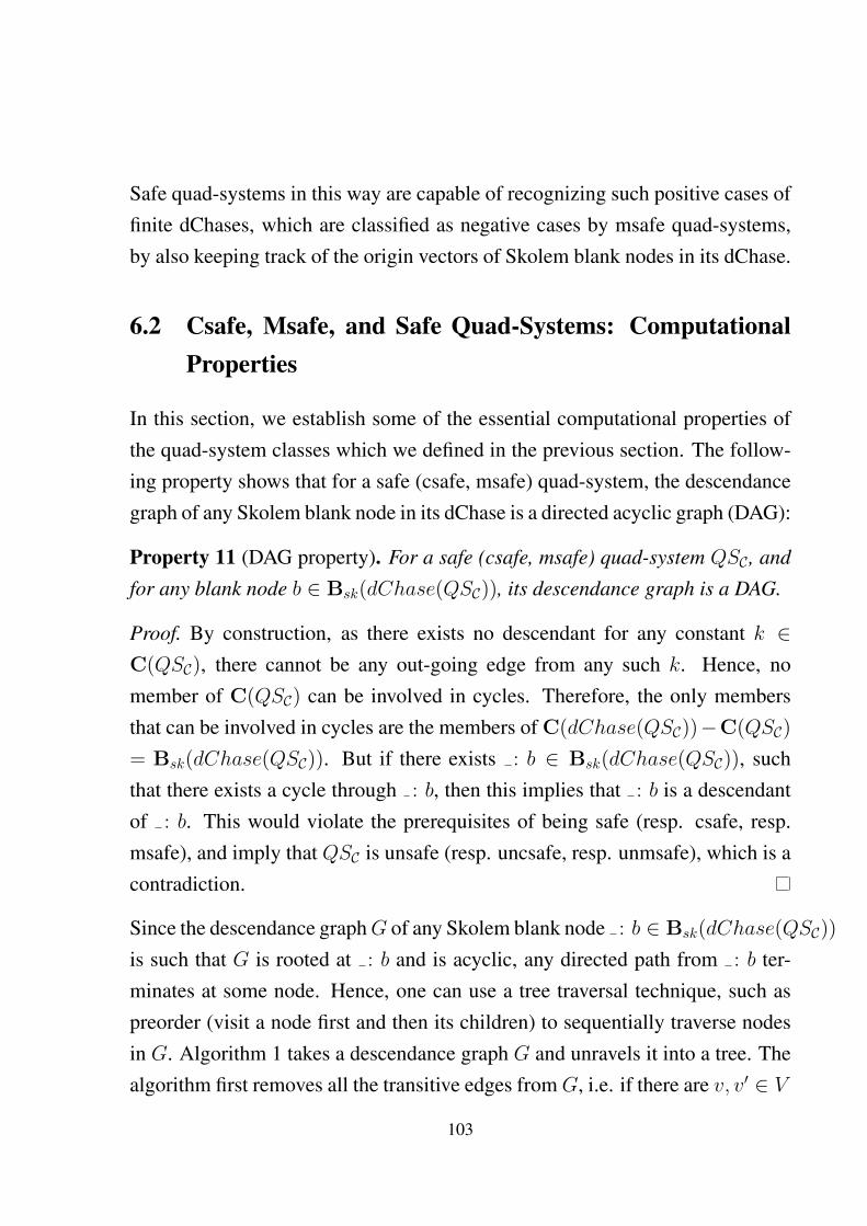
Safe quad-systems in this way are capable of recognizing such positive cases offinite dChases, which are classified as negative cases by msafe quad-systems,by also keeping track of the origin vectors of Skolem blank nodes in its dChase.

6.2 Csafe, Msafe, and Safe Quad-Systems: ComputationalProperties

In this section, we establish some of the essential computational properties ofthe quad-system classes which we defined in the previous section. The follow-ing property shows that for a safe (csafe, msafe) quad-system, the descendancegraph of any Skolem blank node in its dChase is a directed acyclic graph (DAG):

Property 11 (DAG property). For a safe (csafe, msafe) quad-system QSC , and

for any blank node b ∈ Bsk(dChase(QSC)), its descendance graph is a DAG.

Proof. By construction, as there exists no descendant for any constant k ∈C(QSC), there cannot be any out-going edge from any such k. Hence, nomember of C(QSC) can be involved in cycles. Therefore, the only membersthat can be involved in cycles are the members of C(dChase(QSC))−C(QSC)

= Bsk(dChase(QSC)). But if there exists : b ∈ Bsk(dChase(QSC)), suchthat there exists a cycle through : b, then this implies that : b is a descendantof : b. This would violate the prerequisites of being safe (resp. csafe, resp.msafe), and imply that QSC is unsafe (resp. uncsafe, resp. unmsafe), which is acontradiction.

Since the descendance graphG of any Skolem blank node : b ∈ Bsk(dChase(QSC))

is such that G is rooted at : b and is acyclic, any directed path from : b ter-minates at some node. Hence, one can use a tree traversal technique, such aspreorder (visit a node first and then its children) to sequentially traverse nodesin G. Algorithm 1 takes a descendance graph G and unravels it into a tree. Thealgorithm first removes all the transitive edges fromG, i.e. if there are v, v′ ∈ V

103

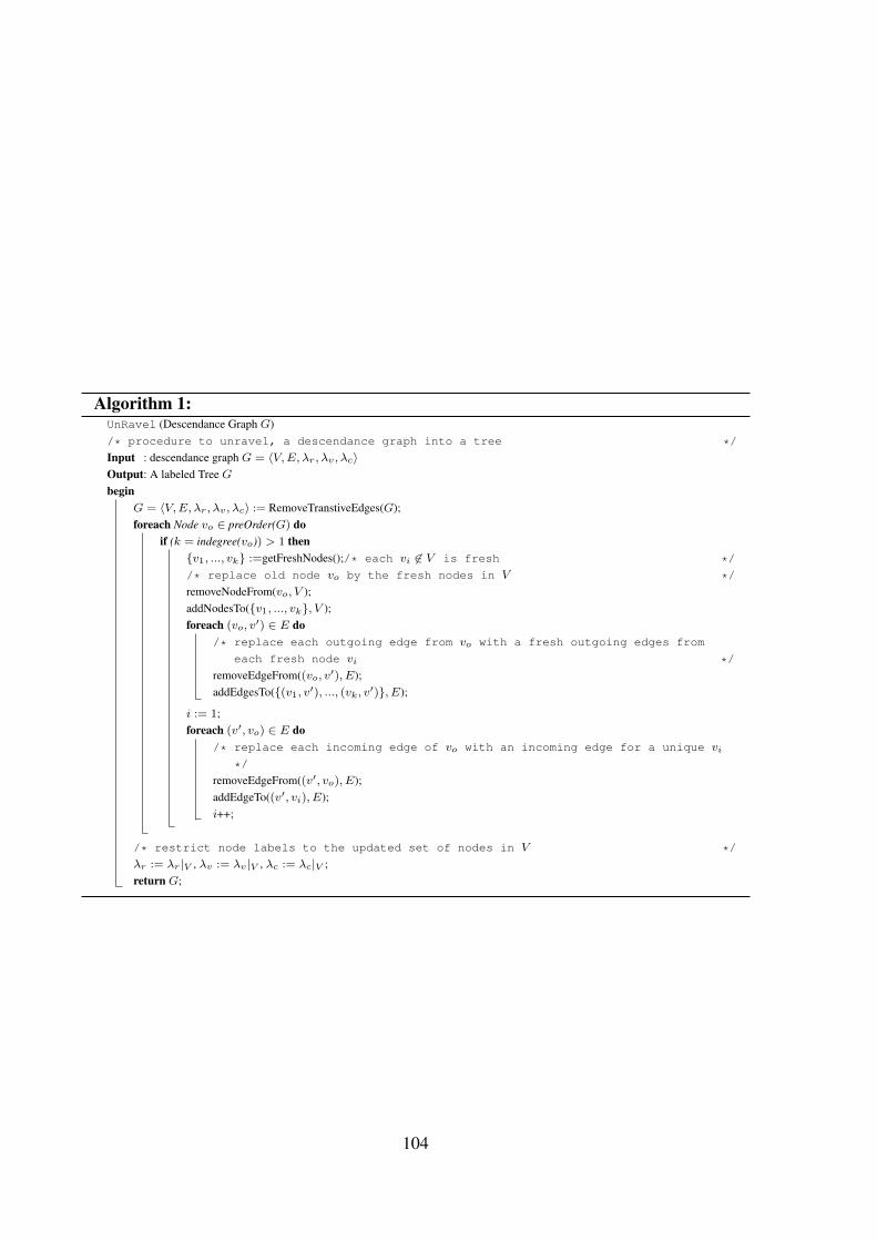
Algorithm 1:UnRavel (Descendance Graph G)/* procedure to unravel, a descendance graph into a tree */

Input : descendance graph G = 〈V,E, λr, λv , λc〉Output: A labeled Tree Gbegin

G = 〈V,E, λr, λv , λc〉 := RemoveTranstiveEdges(G);foreach Node vo ∈ preOrder(G) do

if (k = indegree(vo)) > 1 then{v1, ..., vk} :=getFreshNodes();/* each vi 6∈ V is fresh */

/* replace old node vo by the fresh nodes in V */

removeNodeFrom(vo, V );addNodesTo({v1, ..., vk}, V );foreach (vo, v′) ∈ E do

/* replace each outgoing edge from vo with a fresh outgoing edges from

each fresh node vi */

removeEdgeFrom((vo, v′), E);addEdgesTo({(v1, v′), ..., (vk, v

′)}, E);

i := 1;foreach (v′, vo) ∈ E do

/* replace each incoming edge of vo with an incoming edge for a unique vi

*/

removeEdgeFrom((v′, vo), E);addEdgeTo((v′, vi), E);i++;

/* restrict node labels to the updated set of nodes in V */

λr := λr|V , λv := λv |V , λc := λc|V ;return G;

104

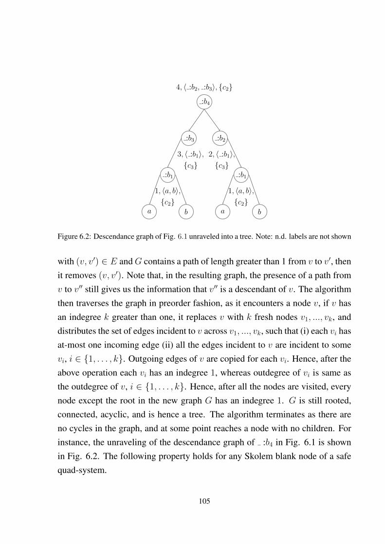
:b4

4, 〈 :b2, :b3〉, {c2}

:b3

3, 〈 :b1〉,{c3}

:b2

2, 〈 :b1〉,{c3}

:b1

1, 〈a, b〉,{c2}

:b1

1, 〈a, b〉,{c2}

a ba b

Figure 6.2: Descendance graph of Fig. 6.1 unraveled into a tree. Note: n.d. labels are not shown

with (v, v′) ∈ E andG contains a path of length greater than 1 from v to v′, thenit removes (v, v′). Note that, in the resulting graph, the presence of a path fromv to v′′ still gives us the information that v′′ is a descendant of v. The algorithmthen traverses the graph in preorder fashion, as it encounters a node v, if v hasan indegree k greater than one, it replaces v with k fresh nodes v1, ..., vk, anddistributes the set of edges incident to v across v1, ..., vk, such that (i) each vi hasat-most one incoming edge (ii) all the edges incident to v are incident to somevi, i ∈ {1, . . . , k}. Outgoing edges of v are copied for each vi. Hence, after theabove operation each vi has an indegree 1, whereas outdegree of vi is same asthe outdegree of v, i ∈ {1, . . . , k}. Hence, after all the nodes are visited, everynode except the root in the new graph G has an indegree 1. G is still rooted,connected, acyclic, and is hence a tree. The algorithm terminates as there areno cycles in the graph, and at some point reaches a node with no children. Forinstance, the unraveling of the descendance graph of :b4 in Fig. 6.1 is shownin Fig. 6.2. The following property holds for any Skolem blank node of a safequad-system.

105

Property 12. For a safe quad-system QSC = 〈QC, R〉, and any Skolem blank

node in dChase(QSC), the unraveling (Algorithm 1) of its descendance graph

results in a tree t = 〈V , E, λr, λv, λc〉 s.t.:

1. any leaf node of t is from the set C(QSC),

2. any non-leaf node of t is from the set Bsk( dChase(QSC)),

3. order(t) ≤ w, where w = maxr∈R|fr(r)|,

4. there cannot be a path between b 6= b′ ∈ V , with λr(b) = λr(b′) and

λv(b) ∼= λv(b′),

5. there cannot be a path between b 6= b′ ∈ V , with λr(b) = λr(b′), if QSC is

also msafe,

6. there cannot be a path between b 6= b′ ∈ V , with λc(b) = λc(b′), if QSC is

also csafe.

Proof. 1. Any node n in the descendance graph is such that n ∈ C(dChase(QSC)),and C(dChase( QSC)) = C(QSC) ] Bsk(dChase(QSC)). Since anymember m ∈ Bsk(dChase(QSC)) is generated from an application of aBR with an assignment µ such that its frontier variables are assigned byµ with a set of constants, m has at-least one child. But, since n is a leafnode, n ∈ C(QSC).

2. Since no member m ∈ C(QSC) can have descendants and any non-leafnode has children, m cannot be a non-leaf node. Hence, non-leaf nodesmust be from Bsk(dChase( QSC)).

3. The order of t is the maximal outdegree among the nodes of t, and outde-gree of a node is the number of children it has. Since any node in t withnon-zero outdegree is a Skolem blank-node : b generated by application

106

of an assignment µ to r = body(r)(~x, ~z)→ head(r)(~x, ~y) ∈ R, the num-ber of children : b has equals ‖~x‖. Hence the order of t is bounded byw.

4. Since any path from b to b′ implies that b′ is a descendant of b, it must bethe case that λr(b) 6= λr(b

′) or λv(b) 6∼= λv(b′), otherwise safety condition

would be violated.

5. Similar as above, immediate by definition.

6. Similar as above, immediate by definition.

The property above is exploited to show that there exists a finite bound in thedChase size and its computation time.

Lemma 13. For any safe/msafe/csafe quad-system QSC = 〈QC , R〉, the follow-

ing holds: (i) the dChase size ‖dChase(QSC)‖=O(22‖QSC‖), (ii) dChase(QSC)

can be computed in 2EXPTIME, (iii) if ‖R‖ and the set of schema triples in

QC is fixed to a constant, then ‖dChase(QSC)‖ is a polynomial in ‖QSC‖ and

can be computed in PTIME.

Proof. The proofs are provided for safe quad-systems, but since CSAFE⊂ MSAFE

⊂ SAFE and since we are giving upper bounds, they also propagate trivially tomsafe and csafe quad-systems.

(i) For any blank node in dChase(QSC), the size of its originVector is upperbounded by w = maxr∈R|fr(r)|. If S is the set of all origin vectors of blank-nodes in dChase(QSC), then cardinality of the set S ′ = S\ ∼= is upper boundedby (|U(QSC)| + |L(QSC)| + w)w, which means that |S ′| = O(2‖QSC‖). Also,since the set of origin ruleId labels, Rids, can at most be |R|, the cardinalityof the set Rids × S ′ = O(2‖QSC‖). For the descendance tree t of any Skolemblank node of dChase(QSC), since there cannot be paths in t between distinct band b′, such that originRuleId(b) = originRuleId(b′) and originV ector(b)∼=

107

originV ector(b′), the length of any such path is upper bounded by |Rids× S ′|= O(2‖QSC‖). However, it turns out that the above upper bound provided isloose, as there is the need of additional filter BRs to transform/back-propagatevectors of constants associated with Skolem blank nodes generated by repetitiveapplication of the same BR. For instance, consider the set of BRs in eg: 10.The BR r1 transforms the origin vector to a new vector each time during itsapplication. BRs r2 - r5 deals with back propagation of these vectors back toinput origin vectors of BR r1. Such filter BRs rule out the case of a BR beingapplied to a quad that contains a Skolem blank node that was generated usingthe same BR on an isomorphic origin vector, ensuring that the safety criteriafor Skolem blank-nodes generated is not violated. It turns out that the numberof such filter BRs required is polynomial w.r.t. to the number of descendantswith the same rule id, for a node in t. Hence, it turns out the depth of t ispolynomially bounded by ‖R‖. (Note that depth of t is bounded by |R| formsafe quad-systems. Also since, the set of origin context labels are bounded bythe set of existential variables inR, depth of t is bounded by ‖R‖ for csafe quad-systems.) Also order of the tree is bounded by w. Hence, any such tree can haveat most O(2‖QSC‖) leaf nodes, O(2‖QSC‖) inner nodes, and O(2‖QSC‖) nodes.Since each of the leaf nodes can only be from C(QSC) and each of the innernodes correspond to an existential variable in R, the number of such possibletrees are clearly bounded double exponentially in ‖QSC‖, hence bounds thenumber of Skolem blank nodes generated in the dChase.

(ii) From (i) ‖dChase(QSC)‖ is double exponential in ‖QSC‖, and sinceeach iteration add at-least one quad to its dChase, the number of iterations arebounded double exponentially in ‖QSC‖. Also, by Lemma 3 any iteration i

can be done in time O(‖dChasei−1(QSC)‖‖R‖). Hence, by using (i), we get‖dChasei−1(QSC)‖ = O(22‖QSC‖). Hence, we can infer that each iteration i canbe done in time O(2‖R‖∗2

‖QSC‖). Also since the number of iterations is at mostdouble exponential, computing dChase(QSC) is in 2EXPTIME.

108

(iii) Since ‖R‖ is fixed to a constant, the set of existential variables is alsoa constant. In this case, since the size of the frontier of any r ∈ R is also aconstant, the order and depth of any descendant tree t of a Skolem blank nodeis a constant. Hence, the number of (leaf) nodes of t is bounded by a constant.Also in this setting, the label of inner nodes of t, which correspond to existentialvariables, is also a constant, and the leaf nodes of t can only be a constantin C(QSC). Hence, the number of descendant trees and consequentially, thenumber of Skolem blank nodes generated is bounded by O(|C(QSC)|z), wherez is a constant. Hence, the set of constants generated in dChase(QSC) is apolynomial in ‖QSC‖, and so is ‖dChase(QSC)‖.

Since in any dChase iteration except the final one, at least one quad is added,and also since the final dChase can have at most O(‖QSC‖z) triples, the totalnumber of iterations are bounded byO(‖QSC‖z) (†). By Lemma 3, since any it-eration i can be computed in O(‖dChasei−1(QSC)‖‖R‖) time, and since ‖R‖ isa constant, the time required for each iteration is a polynomial in ‖dChasei−1(QSC)‖,which is at most a polynomial in ‖QSC‖. Hence, any dChase iteration can beperformed in polynomial time in size of QSC (‡). From (†) and (‡), it can beconcluded that dChase can be computed in PTIME.

Lemma 14. For any safe/msafe/csafe quad-system, the following holds: (i) data

complexity of CCQ entailment is in PTIME, (ii) combined complexity of CCQ

entailment is in 2EXPTIME.

Proof. Note that the proofs are provided for safe quad-systems, but since CSAFE

⊂ MSAFE ⊂ SAFE and since we are giving upper bounds, they also propagatetrivially to msafe and csafe quad-systems.

Given a safe quad-system QSC = 〈QC, R〉, since dChase(QSC) is finite, aboolean CCQ CQ() can naively be evaluated by binding the set of constantsin the dChase to the variables in the CQ(), and then checking if any of thesebindings are contained in dChase(QSC). The number of such bindings can atmost be ‖dChase(QSC)‖‖CQ()‖ (†).

109

(i) Since for data complexity, the size of the BRs ‖R‖, the set of schematriples, and ‖CQ()‖ is fixed to a constant. From Lemma 13 (iii), we know thatunder the above mentioned settings the dChase can be computed in PTIME andis polynomial in the size of QSC . Since ‖CQ()‖ is fixed to a constant, andfrom (†), binding the set of constants in dChase(QSC) on CQ() still gives anumber of bindings that is worst case polynomial in the size of ‖QSC‖. Sincemembership of these bindings can checked in the polynomially sized dChase inPTIME, the time required for CCQ entailment is in PTIME.

(ii) Since in this case ‖dChase(QSC)‖ = O(22‖QSC‖) (‡), from (†) and (‡),binding the set of constants in dChase(QSC) toCQ() amounts toO(2‖CQ()‖∗2‖QSC‖)

number of bindings. Since the dChase is double exponential in ‖QSC‖, check-ing the membership of each of these bindings can be done in 2EXPTIME.Hence, the combined complexity is in 2EXPTIME.

Theorem 15. For any safe/msafe/csafe quad-system, the following holds: (i)

The data complexity of CCQ entailment is PTIME-complete (ii) The combined

complexity of CCQ entailment is 2EXPTIME-complete.

Proof. (i)(Membership) See Lemma 14 for the membership in PTIME.(Hardness) Follows from the PTIME-hardness of data complexity of CCQ en-tailment for Range-Restricted quad-systems (Theorem 3 of Chapter 7), whichare contained in safe/msafe/csafe quad-systems.(ii) (Membership) See Lemma 14.(Hardness) Theorem 16 below shows that the class of context acyclic quad-systems is contained by the class of csafe quad-systems. Since we alreadyshowed that CCQ EP for context acyclic quad-systems is 2EXPTIME-hard, itfollows that CCQ EP is 2EXPTIME-hard for csafe/msafe/safe quad-systems.

The theorem below establishes the fact that the class of csafe quad-systemscontains the class of context acyclic quad-systems defined in the previous sec-

110

tion.

Theorem 16. For any quad-system QSC = 〈QC , R〉, if QSC is context acyclic,

then QSC is csafe.

Proof. We prove the contrapositive, i.e. if a quad-systemQSC is uncsafe, then itis not context acyclic. We, in order to prove the theorem, give a few supportingclaims:

1 If b ∈ C(dChase(QSC)) is a Skolem blank node, then any c∈ originContex-ts(b) is a TGC.

Since b is a Skolem blank node, there exists a BR r= body(r)(~x, ~z)→ head(r)(~x,~y) s.t. b = y[µext(~y)], for some y ∈ {~y}. Hence, any c ∈ originContexts( b)is s.t. c : (s, p, o) ∈ head(~x, ~y), and s or p or o is an existentially quantifiedvariable. This means that any c ∈ originContexts(b) is a TGC.

2 For any quad-system QSC , for any Skolem blank node b, and for any c 6∈originContexts(b), suppose there exists a quad c : (s, p, o) ∈ dChase(QSC),with s = b∨p = b∨o = b, then there exists a path from some ci ∈ originConte-xts(b) to c in the context dependency graph.

Since at any iteration of dChase construction when the Skolem blank node bis introduced in dChase(QSC), originContexts(b) are the only contexts thatcontain a triple in which b occurs. And since the only immediate way by whichb can propagate to any other context c′ 6∈ originContexts(b) in a subsequentiteration is by the application of a BR r ∈ R of the form (4.1), in which someci ∈ originContexts(b) occurs in body(r) and c′ occurs in head(r). Since forany such BR r, there exists an edge from each ci to each c′j, for i ∈ {1, ..., n},j = {1, ...,m} in the context dependency graph, there is a path from somec ∈ originContexts(b) to c′. The claim straightforwardly follows from thegeneralization of the above arguments.

111

For the claim below, we introduce the concept of the sub-distance. For anytwo blank nodes, their sub-distance is inductively defined as:

Definition 17. For any two blank nodes b, b′, sub-distance(b, b′) is defined in-

ductively as:

• sub-distance(b, b′) = 0, if b′ = b;

• sub-distance(b, b′) =∞, if b 6= b′ and b is not a descendant of b′;

• sub-distance(b, b′) = mint∈{~x[µ]}{ sub-distance(b, t)} + 1, if b′ was gener-

ated by application of µ on r = body(r)(~x, ~z)→ head(r)(~x, ~y), i.e. b′ =

yj[µext(~y)], for some yj ∈ {~y}, and b is a descendant of b′.

3 Suppose for any two distinct blank nodes b, b′ ∈ C(dChase(QSC)), if b is adescendant of b′, then there exists a path from c to c′ in the context dependencygraph, for some c ∈ originContexts(b), for every c′ ∈ originContexts(b′).

Suppose if b is a descendant of b′, then it should be the case that sub-distance(b,b′) ∈ N+. We prove this by induction on the value of sub-distance(b, b′).

Base case Suppose sub-distance(b, b′) = 1, that is there exists r = body(r)(~x,~z) → head(r)(~x, ~y) ∈ R, and an assignment µ, with applicableR(r, µ,dChasek(QSC)), b ∈ {~x[µ]}, and b′ is the result of application of µ onr. This means that b occurs in body(r)(~x, ~z)[µ] ⊆ dChasek(QSC), andconsequently there exists a context c with c : (s, p, o) ∈ body(r)(~x, ~z)[µ],with s = b or p = b or o = b, and c : (s, p, o) ∈ dChasek(QSC). Sup-pose c ∈ originContexts(b), then since by construction, there exists anedge from c to every context identifier c′ occuring in head(r), the basecase follows. Otherwise, if c 6∈ originContexts(b), then by Claim 2, itfollows that there exists a path in context dependency graph from somec′ ∈ originContexts(b) to c. Also since there exists an edge from c toevery context identifier c′ occuring in head(r), the base case follows.

112

Hypothesis Suppose sub-distance1 ≤ (b, b′) ≤ k, then there exists a path in thecontext dependency graph, from c to c′, for some c ∈ originContexts(b),for every c′ ∈ originContexts(b′).

Inductive step Suppose sub-distance(b, b′) = k + 1, then this implies thatthere exists a Skolem blank node b′′ s.t. sub-distance(b, b′′) = k and sub-distance(b′′, b′) = 1. From hypothesis it follows that there exists a pathin context dependency graph from some c ∈ originContexts(b) to everyc′′ ∈ originContexts(b′′), and there exists a path in context dependencygraph from some c′′ ∈ originContext(b′′) to every c′ ∈ originContexts(b′).This implies that there exists a path from some c ∈ originContexts(b) toevery c′ ∈ originContexts(b′). Hence, the Claim follows.

Suppose if QSC is uncsafe, then by definition, there exists Skolem blank nodesb, b′ in C(dChase(QSC)), s.t b is a descendant of b′ and originContexts(b)= originContexts(b′). By Claim 3, there exists a path in context dependencygraph from some c ∈ originContexts(b) to every c′ ∈ originContexts(b′).Since originContexts(b) = originContexts(b′), there exists a c ∈ originCo-ntexts(b) s.t. there exists a cycle from c to c it self. Since by Claim 1, ev-ery context in originContexts(b) = originContexts(b′) is a TGC, QSC , bydefinition, is not context acyclic.

6.3 Procedure for Detecting Safe/Msafe/Csafe Quad-Systems

In this subsection, we present a procedure for deciding whether a given quad-system is safe (resp. msafe, resp. csafe) or not. If the quad-system is safe (resp.msafe, resp. csafe), the result of the procedure is a safe dChase (resp. msafe

dChase, csafe dChase) that contains the standard dChase, and can be used forquery answering. Since the safety (resp. msafety, resp. csafety) property ofa quad-system is attributed to the dChase of the quad-system, the procedure

113

nevertheless performs the standard operations for computing the dChase, butalso generate quads that indicate origin ruleIds and origin vectors (resp. originruleIds, resp. origin-contexts) of each Skolem blank node generated. In eachiteration, a test for safety is performed, by checking the presence of Skolemblank-nodes that violate the safety (resp. msafety, resp. csafety) condition.In case a violation is detected, a distinguished quad is generated and the safe(resp. msafe, resp. csafe) dChase construction is aborted, prematurely. Onthe contrary, if there exists an iteration in which no new quad is generated, thesafe (resp. msafe, resp. csafe) dChase computation stops with a completed safe(resp. msafe, resp. csafe) dChase that contains the standard dChase. Since allthe additional quads produced for accounting information use a distinguishedcontext identifier cc 6∈ C, the computed safe (resp. msafe, resp. csafe) dChaseitself can be used for standard query answering. Before geting to the details ofthe procedure, we give a few necessary definitions.

Definition 18 (Context Scope). The context scope of a term t in a set of quad-

patterns Q, denoted by cScope(t, Q) is given as: cScope(t, Q) = {c | c : (s, p,

o) ∈ Q, s = t ∨ p = t ∨ o = t}.

For any quad-system QSC = 〈QC, R〉, let cc be an ad hoc context identifier suchthat cc 6∈ C, then for ri = body(ri)(~x, ~z) → head(ri)(~x, ~y) ∈ R, we definetransformations augS(ri), augM(ri), augC(ri) as follows:

augS(ri) = body(ri)(~x, ~z)→ head(ri)(~x, ~y) ∧ ∀yj ∈ {~y} [∧

xk∈{~x}

cc : (xk,

descendantOf, yj) ∧ cc : (yj, descendantOf, yj) ∧ cc : (yj, originRuleId,

i) ∧ cc : (yj, originVector, ~x)]

It should be noted that cc : (yj, originVector, ~x) is not a valid quad pattern, andis only used for notation brevity. In the actual implementation, vectors can bestored using an rdf container data structure such as rdf:List, rdf:Seq or

114

by typecasting it as a string.

augM(ri) = body(ri)(~x, ~z)→ head(ri)(~x, ~y) ∧ ∀yj ∈ {~y} [∧

xk∈{~x}

cc : (xk,

descendantOf, yj) ∧ cc : (yj, descendantOf, yj) ∧ cc : (yj, originRuleId, i)]

augC(ri) = body(ri)(~x, ~z)→ head(ri)(~x, ~y) ∧ ∀yj ∈ {~y} [∧

xk∈{~x}

cc : (xk,

descendantOf, yj) ∧ cc : (yj, descendantOf, yj) ∧∧

c∈cScope(yj ,head(ri))

cc : (yj,

originContext, c)]

Intuitively, the transformation augS/augM/augC on a BR ri, augments thehead part of ri with additional types of quad patterns, which are the following:

1. cc : (xk, descendantOf, yj), for every existentially quantified variable yj in~y and universally quantified variable xk ∈ {~x}. This is done because,during dChase computation any application of an assignment µ to ri suchthat ~x[µ] = ~a, resulting in the generation of a Skolem blank node : b =

µext(~y)(yj), any ai ∈ {~a} is a descendant of : b. Hence, due to theseadditional quad-patterns, quads of the form cc : (ai, descendantOf, : b)

are also produced, and in this way, keeps track of the descendants of anySkolem blank node produced.

2. cc : (yj, descendantOf, yj), in order to maintain also the reflexivity of ‘de-scendantOf’ relation.

3. cc : (yj, originContext, c), for every existentially quantified variable yj in{~y}, every c ∈ cScope( yj, head(ri)). This is done because during dChasecomputation, any application of an assignment µ on ri, such that ~x[µ] = ~a,resulting in the generation of a Skolem blank node : b = µext(~y)(yj), cis an origin context of : b. Hence due to these additional quad-patterns,

115

quads of the form cc : ( : b, originContext, c) is also produced. In this way,we keep track of the origin-contexts of any Skolem blank node produced.

4. cc : (yj, originVector, ~x), This is done because during the dChase compu-tation, for any application of an assignment µ on ri, such that ~x[µ] = ~a,resulting in the generation of a Skolem blank node : b = µext(~y)(yj), ~ais the origin vector of : b. Hence, due to these additional quad-patterns,quads of the form cc : ( : b, originVector, ~a) is also produced. In this way,we keep track of the origin vector of any Skolem blank node produced.

5. cc : (yj, originRuleId, i), for every existentially quantified variable yj in{~y}, inorder to keep track of the ruleId of the BR used to create any Skolemblank node.

It can be noticed that for any BR ri without existentially quantified variables,the transformations augS/augM/augC leaves ri unchanged. For any set ofBRs R, let

augS(R) (resp. augM(R), resp. augC(R)) =⋃ri∈R

augS(ri) (resp. augM(ri),

resp. augC(ri)) ∪ {cc : (x1, descendantOf, z1) ∧ cc : (z1, descendantOf, x2)→

cc : (x1, descendantOf, x2)}

The function unSafeTest (resp. unMSafeTest, resp. unCSafeTest) defined be-low, given a BR ri = body(ri)(~x, ~z)→ head(ri)(~x, ~y), an assignment µ, and aquad-graphQ checks, if application of µ on ri violates the safety (resp. msafety,resp. csafety) condition on Q.

unSafeTest(ri, µ,Q)=True iff ∃ : b, : b′ ∈ B, with all the following condi-tions being satisfied:

• : b ∈ {~x[µ]}, and

• cc : ( : b′, descendantOf, : b) ∈ Q, and

116

• cc : ( : b′, originRuleId, i) ∈ Q, and

• cc : ( : b′, originVector,~a) ∈ Q, and ~a ∼= ~x[µ].

Intuitively, unSafeTest returns True, if µ applied to ri will produce a freshSkolem blank node : b′′, whose child : b ∈ {~x[µ]}, and according to knowl-edge in Q, : b′ is a descendant of : b such that the origin ruleId of : b′ is i(which is also the origin ruleId of : b′′) and the origin vector of : b′ is isomor-phic to the origin vector of ~x[µ] (which is also the origin vector of : b′′). Thefunctions unMSafeTest and unCSafeTest are similarly defined as follows:unMSafeTest(ri, µ, Q)=True iff ∃ : b, : b′ ∈ B, with all the following condi-tions being satisfied:

• : b ∈ {~x[µ]}, and

• cc : ( : b′,descendantOf, : b) ∈ Q, and

• cc : ( : b′, originRuleId, i) ∈ Q.

unCSafeTest(ri, µ, Q)=True iff ∃ : b, : b′ ∈ B, ∃yj ∈ {~y}, with all the fol-lowing being satisfied:

• : b ∈ {~x[µ]}, and

• cc : ( : b′, descendantOf, : b) ∈ Q, and

• {c | cc : ( : b′, originContext, c) ∈ Q}= cScope( yj, head(ri)(~x, ~y))\{cc}.

For any BR ri and an assignment µ, the safe/msafe/csafe application of µ on riw.r.t. a quad-graph QC is defined as follows:

applysafe(ri, µ,QC) =

{unSafe, If unSafeTest(ri, µ,QC) = True;

apply(ri, µ), Otherwise;

applymsafe(ri, µ,QC) =

{unMSafe, If unMSafeTest(ri, µ,QC) = True;


117

applycsafe(ri, µ,QC) =

{unCSafe, If unCSafeTest(ri, µ,QC) = True;


where unSafe = cc : (unsafe, unsafe, unsafe) (resp. unMSafe = cc : (unmsafe,unmsafe, unmsafe), resp. unCSafe = cc : (uncsafe, uncsafe, uncsafe) is a dis-tinguished quad that is generated, if the prerequisites of safety (resp. msafety,resp. csafety) is violated. For any quad-system QSC = 〈QC, R〉, we define itssafe dChase dChasesafe(QSC) as follows:

dChasesafe0 (QSC) = QC;

dChasesafem+1(QSC) = dChasesafe

m (QSC)∪ applysafe( ri, µ, dChasesafem (QSC)),

if there exists ri ∈ augS(R), assignment µ such that applicableaugS(R)(ri, µ,dChasesafe

m (QSC));

dChasesafem+1(QSC) = dChasesafe

m (QSC), otherwise; for any m ∈ N.

dChasesafe(QSC) =⋃m∈N dChase

safem (QSC)

The termination condition for safe dChase computation can be implementedusing the following conditional: If there exists m such that

dChasesafem (QSC) = dChasesafe

m+1(QSC); then

dChasesafe(QSC) = dChasesafem (QSC).

Similarly, dChases dChasemsafe(QSC) and dChasecsafe( QSC) are defined formsafe and csafe quad-systems, respectively. We bring to the notice of the readerthat although application of any augS(r) (resp. augM(r), resp. augC(r)) pro-duces quad-patterns of the form cc : ( : b, descendantOf, : b), for any Skolemblank node : b generated, there is no raise of a false alarm in the unSafeTest(resp. unMSafeTest, resp. unCSafeTest). This is because unSafeTest (resp. un-MSafeTest, resp. unCSafeTest) on a BR r = body(r)(~x, ~z) → head(r)(~x, ~y)

and assignment µ checks if the application of µ of r with the fresh : b′′ assignedto a yi ∈ {~y} by µext(~y) would have a child : b 6= b′′ assigned to some xi ∈ {~x}by µ, such that there exists a quad of the form cc : ( : b′, descendantOf, : b)

in the safe (resp. msafe, resp. csafe) dChase constructed so far, and : b′′ and: b′ have the same origin ruleId and originVector (resp. originRuleId, resp.

118

originContexts). Note that in the above : b′ should also be distinct from : b′′,and hence rules out the case in which unSafeTest (resp. unMSafeTest, resp.unCSafeTest) returns True because of the detection of a blank node as a selfdescendant of itself.The following theorem shows that the procedure above described for detectingunsafe quad-systems is sound and complete:

Theorem 19. For any quad-system QSC = 〈QC, R〉, the quad unSafe (resp.

unMSafe, resp. unCSafe) ∈ dChasesafe(QSC) (resp. dChasemsafe(QSC), resp.

dChasecsafe(QSC)), iff QSC is unsafe (resp. unmsafe, resp. uncsafe).

It should be noted that for any quad-system QSC = 〈QC , R〉, dChasesafe(QSC)

(resp. dChasemsafe(QSC), resp. dChasecsafe(QSC)) is a finite set and hence theiterative procedure which we described earlier terminates, regardless of whetherQSC is safe (resp. msafe, resp. csafe) or not. This is because ifQSC is safe (resp.msafe, resp. csafe), then, as we have seen before, there exists a double expo-nential bound on number of quads in its dChase. Hence, there is an iterationin which no new quad is generated, which leads to stopping of computation.Otherwise, if QSC is unsafe (resp. msafe, resp. csafe), then from Theorem 19,we know that the quad unSafe (resp. unMSafe, resp. unCSafe) gets gener-ated in dChasesafe(QSC) (resp. dChasemsafe(QSC), resp. dChasecsafe(QSC))in not more than O(22‖QSC‖) iterations. This implies that there exists an it-eration m such that the quad unSafe (resp. unMSafe, resp. unCSafe) is indChasesafe

m (QSC) (resp. dChasemsafem (QSC), resp. dChasecsafe

m (QSC)). W.l.o.g,let m be the first such iteration. This means that there exists a BR ri ∈ R withhead head(ri)(~x, ~y), assignment µ such that applicableaugS(R)(ri, µ, dChas-esafem−1(QSC)) (resp. applicableaugM(R)(ri, µ, dChasemsafe

m−1 (QSC)), resp. applic-ableaugC(R)(ri, µ, dChasecsafe

m−1(QSC)) holds. By construction, since head(ri)[µext(~y)]

is not generated, and instead the quad unSafe (resp. unMSafe, resp. unCSafe)is generated, applicableaugS(R)(ri, µ, dChasesafe

m (QSC)) (resp. applicableaugM(R)(ri,µ, dChasemsafe

m (QSC)), resp. applicableaugC(R)( ri, µ, dChasecsafem (QSC)) holds

119

yet again. This means that the termination condition is satisfied at iterationm + 1, and hence computation stops. Note that regardless of whether a givenquad-system is safe (resp. msafe, resp. csafe) or not, the number of safe (resp.msafe, resp. csafe) dChase iterations is double exponentially bounded in thesize of the quad-system. Consequently, we derive the following theorem.

Theorem 20. Recognizing whether a quad-system is safe/ msafe/csafe is in

2EXPTIME.

Also notice that after running procedure described above, if the quad unSafe(resp. unMSafe, resp. unCSafe) is not generated, then its safe (resp. msafe,resp. csafe) dChase itself can be used for CCQ answering, as in such a casethe standard dChase is contained in safe (resp. msafe, resp. csafe) dChase, andall the quads generated for accounting information have the context identifiercc. Hence, for any safe (resp. msafe, resp. csafe) quad-system, for any booleanCCQ that does not contain quad patterns of the form cc : (s, p, o), the dChaseentails CCQ iff the safe (resp. msafe, resp. csafe) dChase entails CCQ.

A set of BRs R is said to be universally safe (resp. msafe, resp. csafe) iff,for any quad-graph QC , the quad-system 〈QC, R〉 is safe (resp. msafe, resp.csafe). For any set of BRs R, whose set of context identifiers is C, also letUR be the set of URIs that occur in the triple patterns of R plus an additionalad hoc blank node : bcrit, the critical quad-graph of R is defined as the set{c : (s, p, o)|c ∈ C, {s, p, o} ⊆ UR}. The following property illustrates how thecritical quad-graph of a set of BRs R can be used to determine, whether or notR is universally safe/msafe/csafe.

Property 21. A set of BRs R is universally safe (resp. msafe, resp. csafe) iff

〈QcritC , R〉 is safe (resp. msafe, resp. csafe), where Qcrit

C is the critical quad-

graph of R.

120

Chapter 7

Range Restricted Quad-Systems

In this chapter, we investigate the complexity of CCQ entailment over quad-systems, whose BRs do not have existentially quantified variables.

7.1 Restricting to Range Restricted BRs

Suppose if we prohibit the occurrence of existentially quantified variables fromthe BRs of the form (4.1), then the resulting BRs must be of the form:

c1 : t1(~x, ~z) ∧ ... ∧ cn : tn(~x, ~z)→ c′1 : t′1(~x) ∧ ... ∧ c′m : t′m(~x)

Note that any set of BRs R of the form above can be replaced by semanticallyequivalent set R′, such that each r ∈ R′ is the form:

c1 : t1(~x, ~z), ..., cn : tn(~x, ~z)→ c′1 : t′1(~x) (7.1)

Also ‖R′‖ is at most quadratic in ‖R‖, and hence, w.l.o.g, we assume that eachr ∈ R is of the form (7.1). Borrowing the parlance from the ∀∃ rules setting,where rules whose variables in the head part are contained in the variables in thebody part are called range restricted rules [6], we call such BRs range restricted

(RR) BRs. We call a quad-system whose BRs are all of RR-type, a RR quad-

system. Since there exists no existentially quantified variables in BRs of a RRquad-system, no Skolem blank nodes are produced during dChase computation.

121

Hence, there can be no violation of the context acyclicity condition in chapter5 and safety/msafety/csafety condition in chapter 6, and hence, the class of RRquad-systems are contained in the class of safe/msafe/csafe quad-systems, andis also a FEC. Of course, this containment is strict as any quad-system thatcontains a BR with an existential variable is not RR. Since one can determinewhether or not a given quad-system is RR or not by simply iterating through setof BRs and checking their syntax, the following holds:

Theorem 1. Recognizing whether a quad-system is RR can be done in linear

time.

In the following, we see that restricting to RR BRs, size of the dChase be-comes polynomial w.r.t. size of the input quad-system, and the complexity ofCCQ entailment further reduces compared to safe/msafe/csafe quad-systems.

Lemma 2. For any RR quad-system QSC = 〈QC, R〉, the following holds: (i)

‖dChase(QSC)‖ = O(‖QSC‖4) (ii) dChase(QSC) can be computed in EXP-TIME (iii) If ‖R‖ is fixed to be a constant, dChase(QSC) can be computed in

PTIME.

Proof. (i) Note that the number of constants in QSC is roughly equal to ‖QSC‖.As no existential variable occurs in any BR in a RR quad-systemQSC , the set ofconstants C(dChase(QSC)) is contained in C(QSC). Since each c : (s, p, o) ∈dChase(QSC) is such that c, s, p, o ∈ C(QSC), |dChase(QSC)| = O(|C(QSC

)|4). Hence ‖dChase(QSC)‖ = O(|C(QSC)|4) = O(‖QSC‖4).

(ii) Since from (i) |dChase(QSC)| = O(‖QSC‖4), and in each iteration ofthe dChase at least one new quad is added, the number of iterations cannotexceedO(‖QSC‖4). Since by Lemma 3, each iteration i of dChase computationrequires O(|R| ∗ ‖dChasei−1( QSC)‖rs) time, where rs = maxr∈R‖r‖, andrs ≤ ‖QSC‖, time required for each iteration is of the order O(2‖QSC‖) time.Although the number of iterations is a polynomial, each iteration requires an

122

exponential amount of time w.r.t ‖QSC‖. Hence time complexity of dChasecomputation is in EXPTIME.

(iii) As we know that the time taken for application of a BR R is O(‖dCha-sei−1(QSC)‖‖R‖). Since ‖R‖ is fixed to a constant, application of R can bedone in PTIME. Hence, each dChase iteration can be computed in PTIME. Alsosince the number of iterations is a polynomial in ‖QSC‖, computing dChase isin PTIME.

Theorem 3. Data complexity of CCQ entailment over RR quad-systems is PTIME-

complete.

Proof. (Membership) Follows from the membership in P of data complexityof CCQ entailment for safe quad-systems, whose expressivity subsumes theexpressivity of RR quad-systems (Theorem 15 of Chapter 6).

(Hardness) In order to prove P-hardness, we reduce a well known P-completeproblem, 3HornSat, i.e. the satisfiability of propositional Horn formulas withat most 3 literals. Note that a (propositional) Horn formula is a propositionalformula of the form:

P1 ∧ . . . ∧ Pn → Pn+1 (7.2)

where Pi, for 1 ≤ i ≤ n + 1, are either propositional variables or constants t,f , that represents true and false, respectively. Note that for any propositionalvariable P , the fact that “P holds” is represented by the formula t → P , and“P does not hold” is represented by the formula P → f . A 3Horn formula isa formula of the form (7.2), where 1 ≤ n ≤ 2. Note that any (set of) Hornformula(s) Φ can be transformed in polynomial time to a polynomially sized setΦ′ of 3Horn formulas, by introducing auxiliary propositional variables such thatΦ is satisfiable iff Φ′ is satisfiable. A pure 3Horn formula is a 3Horn formulaof the form (7.2), where n = 2. Any 3Horn formula φ that is not pure can betrivially converted to equivalent pure form by appending a ∧ t on the body part

123

of φ. For instance, P → Q, can be converted to P ∧ t→ Q. Hence, w.l.o.g. weassume that any set of 3Horn formulas is pure, and is of the form:

P1 ∧ P2 → P3 (7.3)

In the following, we reduce the satisfiability problem of pure 3Horn formulas toCCQ entailment problem over a quad-system whose set of schema triples, theset of BRs, and the CCQ CQ are all fixed.

For any set of pure Horn formulas Φ, we construct the quad-system QSC =

〈QC, R〉, where C = {ct, cf}. For any formula φ ∈ Φ of the form (7.3), QC con-tains a quad cf : (P1, P2, P3). In additionQC contains a quad ct : (t, rdf:type,T ). R is the singleton that contains only the following fixed BR:

ct : (x1,rdf:type, T ), ct : (x2,rdf:type, T ),

cf : (x1, x2, x3)→ ct : (x3,rdf:type, T )

Let the CQ be the fixed query ct : (f,rdf:type, T ).Now, it is easy to see that QSC |= CQ, iff Φ is not satisfiable.

Theorem 4. Combined complexity of CCQ entailment over RR quad-systems is

in EXPTIME.

Proof. (Membership) By Lemma 2, for any RR quad-system QSC , its dChasedChase(QSC) can be computed in EXPTIME. Also by Lemma 2, its dChasesize ‖dChase(QSC)‖ is a polynomial w.r.t to ‖QSC‖. A boolean CCQ CQ()

can naively be evaluated by grounding the set of constants in the dChase tothe variables in the CQ(), and then checking if any of these groundings arecontained in dChase(QSC). The number of such groundings can at most be‖dChase(QSC)‖‖CQ()‖ (†). Since ‖dChase(QSC)‖ is a polynomial in ‖QSC‖,there are an exponential number of groundings w.r.t ‖CQ()‖. Since contain-ment of each of these groundings can be checked in time polynomial w.r.t. thesize of dChase(QSC), and since ‖dChase(QSC)‖ is a polynomial w.r.t. ‖QSC‖,the time complexity of CCQ entailment is in EXPTIME.

124

Concerning the combined complexity of CCQ entailment of RR quad-systems,we leave the lower bounds open.

7.2 Restricted RR Quad-Systems

We call those quad-systems with BRs of form (7.1) with a fixed bound on n asrestricted RR quad-systems. They can be further classified as linear, quadratic,cubic,..., quad-systems, when n = 1, 2, 3, ..., respectively.

Theorem 5. Data complexity of CCQ entailment over restricted RR quad-systems

is P-complete.

Proof. The proof is same as in Theorem 3, since the size of BRs are fixed toconstant.

Theorem 6. Combined complexity of CCQ entailment over restricted RR quad-

systems is NP-complete.

Proof. Let the problem of deciding if QSC |= CQ() be called DP’.(Membership) for any QSC whose rules are of restricted RR-type, the size

of any r ∈ R is a constant. Hence, by Lemma 3, any dChase iteration canbe computed in PTIME. Since the number of iterations is also polynomial in‖QSC‖, dChase(QSC) can be computed in PTIME in the size of QSC anddChase(QSC) has a polynomial number of constants. Hence, we can guessan assignment µ for all the existential variables in CCQ CQ(), to the set ofconstants in dChase(QSC). Then, one can evaluate the CCQ, by checking ifc : (s, p, o) ∈ dChase(QSC), for each c : (s, p, o) ∈ CQ()[µ], which can bedone in timeO(‖CQ‖ ∗ ‖dChase(QSC)‖), and is hence is in non-deterministicPTIME, which implies that DP’ is in NP.

(Hardness) We show that DP’ is NP-hard, by reducing the well known NP-hard problem of 3-colorability to DP’. Given a graph G = 〈V , E〉, where V =

{v1, ..., vn} is the set of nodes, E ⊆ V ×V is the set of edges, the 3-colorability

125

problem is to decide if there exists a labeling function l : V → {r, b, g} thatassigns each v ∈ V to an element in {r, b, g} such that the condition: (v, v′) ∈E → l(v) 6= l(v′), for each (v, v′) ∈ E, is satisfied.

One can construct a quad-system QSc = 〈Qc, ∅〉, where graphQc(c) has the

following triples:{(r, edge, b), (r, edge, g), (b, edge, g), (b, edge, r), (g, edge, r), (g, edge, b)}

Let CQ be the boolean CCQ: ∃v1, ...., vn∧

(v,v′)∈E [ c : (v, edge, v′) ∧ c : (v′,edge, v)]. Then, it can be seen that G is 3-colorable, iff QSc |= CQ.

126

Chapter 8

Quad-Systems vs Forall-Existential rules

In this section, we formally compare the formalism of quad-systems with forall-existential (∀∃) rules. In the realm of ∀∃ rule sets, a conjunctive query (CQ) isan expression of the form:

∃~y p1(~x, ~y) ∧ ... ∧ pr(~x, ~y) (8.1)

where pi(~x, ~y), for 1 ≤ i ≤ r are predicate atoms over vectors ~x or ~y. A booleanCQ is defined as usual. The decision problem of whether, for a ∀∃ rule set Pand a CQ Q, if P |=fol Q is called the CQ EP, where |=fol is the standard firstorder logic entailment relation.

For any quad-graph QC = {c1 : (s1, p1, o1), . . . , cn : (sr, pr, or)}, let rQC bethe BR

→ ~∃yb1, . . . , ybq c1 : (s1, p1, o1)[µB] ∧ . . . ∧ cr : (sr, pr, or)[µB],

where { : b1, . . . , : bq} is the set of blank nodes in QC , and µB is the sub-stitution function { : bi → ybi}i=1,...,q that assigns each blank-node to a freshexistentially quantified variable. It can be noted that the quad-systems 〈QC, R〉and 〈∅, R ∪ {rQC}〉 are semantically equivalent. The following definition givesthe translation functions that will be necessary to establish the relation betweenquad-systems and ∀∃ rule sets.

127

Definition 1 (Translations τq, τr, τccq, τ ). The translation function τq from the set

of quad patterns to the set of ternary atoms is defined as: for any quad-pattern

c : (s, p, o), τq(c : (s, p, o)) = c(s, p, o).

The translation function τbr from the set of BRs to the set of ∀∃ rules is

defined as: for any BR r of the form (4.1):

τbr(r) = ∀~x∀~z [τq(c1 : t1(~x, ~z)) ∧ ... ∧ τq(cn : tn(~x, ~z))→

∃~y τq(c′1 : t′1(~x, ~y)) ∧ ... ∧ τq(c′m : t′m(~x, ~y))],

The translation function τ from the set of quad-systems to forall-existential

rule sets is defined as: for any quad-systemQSC = 〈QC, R〉, τ(QSC) = τbr(R)∪{τbr(rQC)}, where τbr(R) =

⋃r∈R τbr(r).

The translation function τccq from the set of boolean CCQs to the set of

boolean CQs is defined as: for any boolean CCQ CQ = ∃~y c1 : t1(~a, ~y) ∧ . . .∧cr : tr(~a, ~y), τccq(CQ) is:

∃~y τq(c1 : t1(~a, ~y)) ∧ . . . ∧ τq(cr : tr(~a, ~y)).

The following property gives the relation between CCQ entailment of unre-stricted quad-systems and standard first order CQ entailment of ∀∃ rule sets.

Property 2. For any quad-system QSC , CCQ CQ, QSC |= CQ iff τ(QSC) |=fol

τccq(CQ).

Proof. Notice that every context c ∈ C becomes a ternary predicate symbol inthe resulting translation. Also, τ(QSC) is a ∀∃ rule set, and for any CCQ CQ,τccq(CQ) is a CQ.

In order to construct the restricted chase for τ(QSC), suppose that ≺q is alsoextended to set of instances such that for any two quad-graphs QC , Q′C′, QC ≺qQ′C′ iff τq(QC) ≺q τq(Q′C′). Suppose ≺ is extended similarly to set of instances.Also assume that during the construction of standard chase chase(τ(QSC)) ofτ(QSC), for any application of a τbr(r) with existentially quantified variables,

128

with r ∈ R, suppose the Skolem blank nodes generated in chase(τ(QSC))

follow the same order as they are generated in dChase( QSC). Also let usextend the rule applicability function to the ∀∃ rules settings such that for any setof BRs R, for any r ∈ R, quad-graph Q′C′, assignment µ, applicableR(r, µ,Q′C′)

iff applicableτbr(R)(τbr(r), µ, τq(Q′C′)).Now it can be seen that dChase0(〈∅, R ∪ {rQC}〉) = ∅, chase0(τ(QSC))

= ∅, dChase1(QSC) = apply(rQC , µ∅), where µ∅ is the empty function, andchase1(τ(QSC)) = apply(τbr(rQC), µ∅), and so on. It is straightforward to seethat, for anym ∈ N, τq( dChasem(〈∅,R∪{rQC}〉)) = chasem(τ(QSC)). Conse-quently, τq(dChase(QSC)) = chase(τ(QSC)), and {CQ}[σ] ⊆ dChase(QSC)

iff {τccq( CQ)}[σ] ⊆ chase(τ(QSC)).Hence, applying Theorem 2 of Chapter 6 and the analogous theorem for ∀∃

rulesets from Deutch et al. [35], it follows that for any quad-systemQSC = 〈QC ,R〉 and a boolean CCQ CQ, QSC |= CQ iff τ(QSC) |=fol τccq(CQ).

Theorem 3. There exists a polynomial time translation function τ (resp. τccq)

from the set of unrestricted quad-systems (resp. CCQs) to the set of ∀∃ rule sets

(resp. CQs), such that for any unrestricted quad-system QSC and a CCQ CQ,

QSC |= CQ iff τ(QSC) |=fol τccq(CQ).

Proof. It is easy to see that τq, τbr, τ , and τccq in Definition 1 can be imple-mented using simple syntax transformation, by iterating through the respectivecomponents of a quad-system/CCQ, and the time complexity of these functionsare linear w.r.t their inputs.

Notice that for any CCQ CQ (resp. CQ Q), → CQ (resp. → Q) is a bridge(resp. ∀∃) rule, with an empty body. Also, since for any quad-graph QC , thetranslation function τbr defined above can directly be applied on rQC to obtain a∀∃ rule, the following theorem immediately follows:

Theorem 4. For quad-systems, the EPs: (i) quad EP, (ii) quad-graph EP, (iii)

BR EP, (iv) BRs EP, (v) Quad-System EP, and (vi) CCQ EP are polynomially

129

reducible to entailment of ∀∃ rule sets.

A ∀∃ rule set P is said to be a ternary ∀∃ rule set, iff all the predicate symbolsin the vocabulary of P are of arity less than or equal to three. P is a purely

ternary rule set, iff all the predicate symbols in the vocabulary P is of aritythree. Similarly, a (purely) ternary CQ is defined. The following property givesthe relation between the CQ entailment problem of ∀∃ rule sets and CCQ EP ofunrestricted quad-systems.

Theorem 5. There exists a polynomial time tranlation function ν (resp. νcq)

from ternary ∀∃ rule sets (resp. ternary CQs) to unrestricted quad-systems

(resp. CCQs) such that for any ternary ∀∃ rule set P and a ternary CQ Q, P|=fol CQ iff 〈∅, ν(P)〉 |= νcq(Q).

Proof. Note that the CQ EP of any ternary ∀∃ rule set P, whose set of predicatesymbols is P , and CQ Q over P , can polynomially reduced to the CQ EP of apurely ternary rule set P′ and purely ternary CQ Q′, by the following transfor-mation function χ. Let � be an adhoc fresh URI; χ is such that for any ternaryatom c(s, p, o), χ(c(s, p, o)) = c(s, p, o). For any binary atom c(s, p), χ(c(s, p))

= c(s, p,�), and for any unary atom c(s), χ(c(s)) = c(s,�,�). For any ∀∃rule r of the form (2.2),

χ(r) = ∀~x∀~z [χ(p1(~x, ~z)) ∧ . . . ∧ χ(pn(~x, ~z))

→ ∃~y χ(p′1(~x, ~y)) ∧ . . . ∧ χ(p′m(~x, ~y))]

And, for any ∀∃ rule set P, χ(P) =⋃r∈P χ(r). For any CQ Q, χ(Q) is similarly

defined. Note that for any ternary ∀∃ rule set P, ternary CQ Q, χ(P) (resp.χ(Q)) is purely ternary, and P |=fol Q iff χ(P) |=fol χ(Q).

Also, it can straightforwardly seen that τ−1br (χ(P)) (resp. τ−1

ccq (χ(Q))) is a setof BRs (resp. CCQ). Suppose, ν(P) is such that ν(P) = QSC = 〈∅, τ−1

br (χ(P))〉.Intuitively, C contains a context identifier c, for each predicate symbol c ∈P . Also suppose, νcq(Q) = τ−1

ccq (χ(Q)). Notice that νcq(Q) is CCQ. It can

130

straightforwardly seen that ν and νcq can be computed in polynomial time, andP |=fol Q iff ν(P) |= νcq(Q).

Thanks to Theorem 3 and Theorem 5, the following theorem immediately holds:

Theorem 6. The CCQ EP over quad-systems is polynomially equivalent to CQ

EP over ternary ∀∃ rule sets.

By virtue of the theorem above, we derive the following property:

Property 7. For quad-systems, the Quad EP, Quad-graph EP, BR(s) EP, and

Quad-system EP are polynomially reducible to CCQ EP.

Proof. The following claim is a folklore in the realm of ∀∃ rules.

Claim (1) The ∀∃ rule set EP is polynomially reducible to CQ EP.

Reducibility of ∀∃ rule EP to CQ EP is a folklore in the realm of ∀∃ rules. For aformal proof, we refer the reader to Baget et al. [6], where it is shown that the ∀∃rule EP is polynomially reducible to fact (a set of instances) EP, and fact EP areequivalent to CQ EP. Also, Cali et al [21] show that CQ containment problem,which is equivalent to ∀∃ rule EP, is reducible to CQ EP. Since a ∀∃ rule set is aset of ∀∃ rules, by using a series of oracle calls to a function that solves the ∀∃rule EP, we can define a function for deciding ∀∃ rule set entailment. Hence,the claim holds.

(a) Thanks to translation functions τ , τbr defined earlier, such that for anyquad-system QSC , quad-graph Q′C′, QSC |= Q′C′ iff τ(QSC) |=fol τbr(rQ′

C′), we

can infer that quad-graph EP is polynomially reducible to ∀∃ rule set EP. Ap-plying claim 1, it follows the quad-graph EP over quad-systems is polynomiallyreducible to CQ EP over ∀∃ rule sets. By Theorem 5, we can deduce that quad-graph EP is polynomially reducible to CCQ EP.

(b) By the translation functions τ and τbr, defined earlier, such that for anyquad-system QSC , a set of BRs R, QSC |= R iff τ(QSC) |=fol τbr(R), we can

131

infer that BRs EP is polynomially reducible to ∀∃ rule set EP. Similar to (a)above, we deduce that BRs EP is polynomially reducible to CCQ EP.

From (a) and (b), it follows that Quad-system EP is reducible to CCQ EP.

Having seen that the CCQ EP over quad-systems is polynomially equivalentto CQ EP over ternary ∀∃ rule sets, we now compare some of the well knowntechniques used to ensure decidability of CQ entailment in the ∀∃ rules settingsto the decidability techniques for quad-systems that we saw earlier in the pre-vious sections. Note that since all the quad-system classes we proposed in thispaper are FECs, for a judicious comparison, the ∀∃ rule classes to which wecompare are classes which have a finite chase property. We compare to the fol-lowing three well known classes: (i) Weakly Acyclic rule sets (WA), (ii) JointlyAcyclic rule sets (JA), and (iii) Model Faithful Acyclic ∀∃ rule sets (MFA). Thefollowing property is well known in the realm of ∀∃ rules:

Property 8. For the any ∀∃ rule set P, the following holds:

1. If P ∈ WA, then P ∈ JA (from [60]),

2. If P ∈ JA, then P ∈ MFA (from [32]),

3. WA ⊂ JA ⊂ MFA (from [60] and [32]).

Note that a description of few other ∀∃ rule classes that do not have the finitechase property, but still enjoy decidability of CQ entailment are given in therelated work.

8.1 Weak Acyclicity

Weak acyclicity [39, 34] is a popular technique used to detect whether a ∀∃ ruleset has a finite chase, thus ensuring decidability of query answering. The set WA

represents class of ternary ∀∃ rule sets that have the weak acyclicity property.

132

For any predicate atom p(t1, . . . , tn), an expression 〈p, i〉, for i = 1, . . . , n iscalled a position of p. In the above case, t1 is said to occur at position 〈p, 1〉,t2 at 〈p, 2〉, and so on. For a set of ∀∃ rules P, its dependency graph is a graphwhose nodes are positions of predicate atoms in P; for each r ∈ P of the form(2.2), and for any variable x occurring in position 〈p, i〉 in head of r:

1. if x is universally quantified and x occurs in the body of r at position〈p′, j〉, then there exists an edge from 〈p′, j〉 to 〈p, i〉

2. if x is existentially quantified, then for any universally quantified variablex′ occurring in the head of r, with x′ also occurring in the body of r atposition 〈p′, j〉, there exists a special edge from 〈p′, j〉 to 〈p, i〉.

P is called weakly acyclic, iff its dependency graph does not contain cycles go-ing through a special edge. For any ∀∃ rule set P, if P is WA, then its chase isfinite, and hence CQ EP is decidable. Note that the nodes in the dependencygraph that has incoming special edges corresponds to the positions of predi-cates where new values are created due to existential variables, and the normaledges capture the propagation of constants from one predicate position to an-other predicate position. In this way, absence of cycles involving special edgesensures that newly created Skolem blank nodes are not recursively used to cre-ate other new Skolem blank nodes in the same position, leading to terminationof chase computation.

Theorem 9. Let τ be the translation function from the set of unrestricted quad-

systems to the set of ternary ∀∃ rule sets, as defined in property 2, then, for any

quad-system QSC = 〈QC , R〉, the following holds: (i) if QSC is context acyclic,

then τ(QSC) is weakly acyclic; the converse may not hold, in general, (ii) if

local semantics of contexts is OWL-Horst or its derivative, i.e. OWL-Horst IRs

⊆ LIR, then QSC is context acyclic iff τ(QSC) is weakly acyclic.

Proof. (i) We prove the contrapositive, i.e. suppose τ(QSC) is not weaklyacyclic, then QSC is not context acyclic. By construction of dependency graph,

133

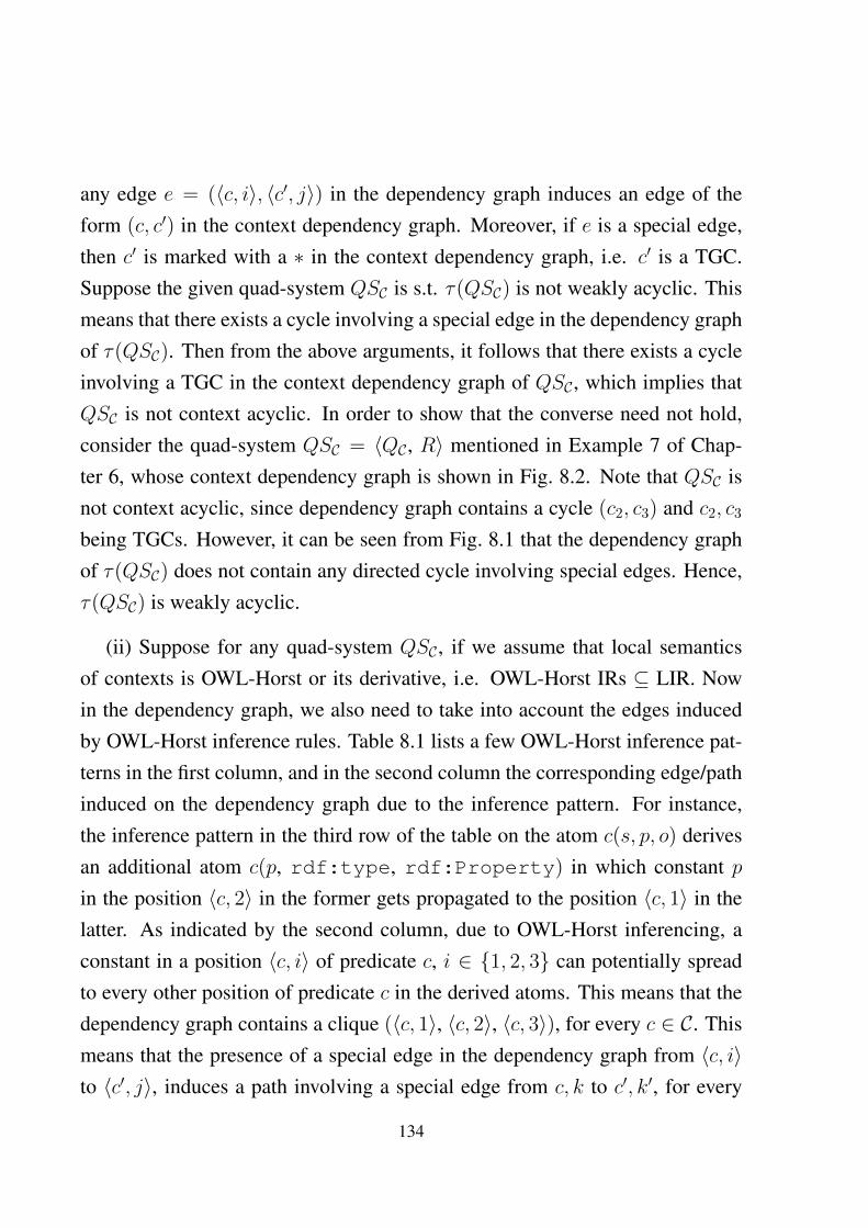
any edge e = (〈c, i〉, 〈c′, j〉) in the dependency graph induces an edge of theform (c, c′) in the context dependency graph. Moreover, if e is a special edge,then c′ is marked with a ∗ in the context dependency graph, i.e. c′ is a TGC.Suppose the given quad-system QSC is s.t. τ(QSC) is not weakly acyclic. Thismeans that there exists a cycle involving a special edge in the dependency graphof τ(QSC). Then from the above arguments, it follows that there exists a cycleinvolving a TGC in the context dependency graph of QSC , which implies thatQSC is not context acyclic. In order to show that the converse need not hold,consider the quad-system QSC = 〈QC , R〉 mentioned in Example 7 of Chap-ter 6, whose context dependency graph is shown in Fig. 8.2. Note that QSC isnot context acyclic, since dependency graph contains a cycle (c2, c3) and c2, c3

being TGCs. However, it can be seen from Fig. 8.1 that the dependency graphof τ(QSC) does not contain any directed cycle involving special edges. Hence,τ(QSC) is weakly acyclic.

(ii) Suppose for any quad-system QSC , if we assume that local semanticsof contexts is OWL-Horst or its derivative, i.e. OWL-Horst IRs ⊆ LIR. Nowin the dependency graph, we also need to take into account the edges inducedby OWL-Horst inference rules. Table 8.1 lists a few OWL-Horst inference pat-terns in the first column, and in the second column the corresponding edge/pathinduced on the dependency graph due to the inference pattern. For instance,the inference pattern in the third row of the table on the atom c(s, p, o) derivesan additional atom c(p, rdf:type, rdf:Property) in which constant pin the position 〈c, 2〉 in the former gets propagated to the position 〈c, 1〉 in thelatter. As indicated by the second column, due to OWL-Horst inferencing, aconstant in a position 〈c, i〉 of predicate c, i ∈ {1, 2, 3} can potentially spreadto every other position of predicate c in the derived atoms. This means that thedependency graph contains a clique (〈c, 1〉, 〈c, 2〉, 〈c, 3〉), for every c ∈ C. Thismeans that the presence of a special edge in the dependency graph from 〈c, i〉to 〈c′, j〉, induces a path involving a special edge from c, k to c′, k′, for every

134

OWL-Horst inference pattern Induced edgesc(x1,owl:equivalentProperty, z), c(x2, z, x3)→ c(x2, x1, x3) 〈c, 1〉 → 〈c, 2〉c(x,rdf:type,rdfs:Class)→ c(x,rdfs:subClassOf, x) 〈c, 1〉 → 〈c, 3〉c(z1, x, z2)→ c(x,rdf:type,rdf:Property) 〈c, 2〉 → 〈c, 1〉c(z1, x, z2)→ c(x,rdf:type,rdf:Property)→ c(x, 〈c, 2〉 → 〈c, 3〉rdfs:subPropertyOf, x)

c(z1, z2, x)→ c(x,rdf:type,rdfs:Resource) 〈c, 3〉 → 〈c, 1〉c(z,rdfs:subPropertyOf, x1), c(x2, z, x3)→ c(x2, x1, x3) 〈c, 3〉 → 〈c, 2〉

Table 8.1: Edges induced in the dependency graph due to OWL-Horst inferencing

k, k′ ∈ {1, 2, 3}. From these facts, suppose if a given quad-system QSC is notcontext acyclic, then by definition its context dependency graph contains a cyclethrough a TGC. Due to the above arguments, the dependency graph of τ(QSC)

should contain a cycle involving a special edge. This implies that QSC is notweakly acyclic. The converse follows from (i).

Example 10. Let us revisit the quad-system QSC = 〈QC , R〉 mentioned in Ex-ample 7 of Chapter 6, whose dependency graph is shown in Fig. 8.1. Note thatthe QSC is uncsafe, since its dChase contains a Skolem blank-node : b4, whichhas as descendant another Skolem blank node : b1, with the same origin con-text c2 (see Fig. 6.1). However, it can be seen from Fig. 8.1 that the dependencygraph of τ(QSC) does not contain any directed cycle involving special edges.Hence τ(QSC) is weakly acyclic.

It turns out that there exists no inclusion relationship between the classesWA and CSAFE in either directions, i.e. WA 6⊆ CSAFE (from example 10), andCSAFE 6⊆ WA (from the fact that WA ⊂ JA, and example 11 below). WhereasWA ⊂ MSAFE, since WA ⊂ MFA and MFA ≡ MSAFE (theorem 12).

135

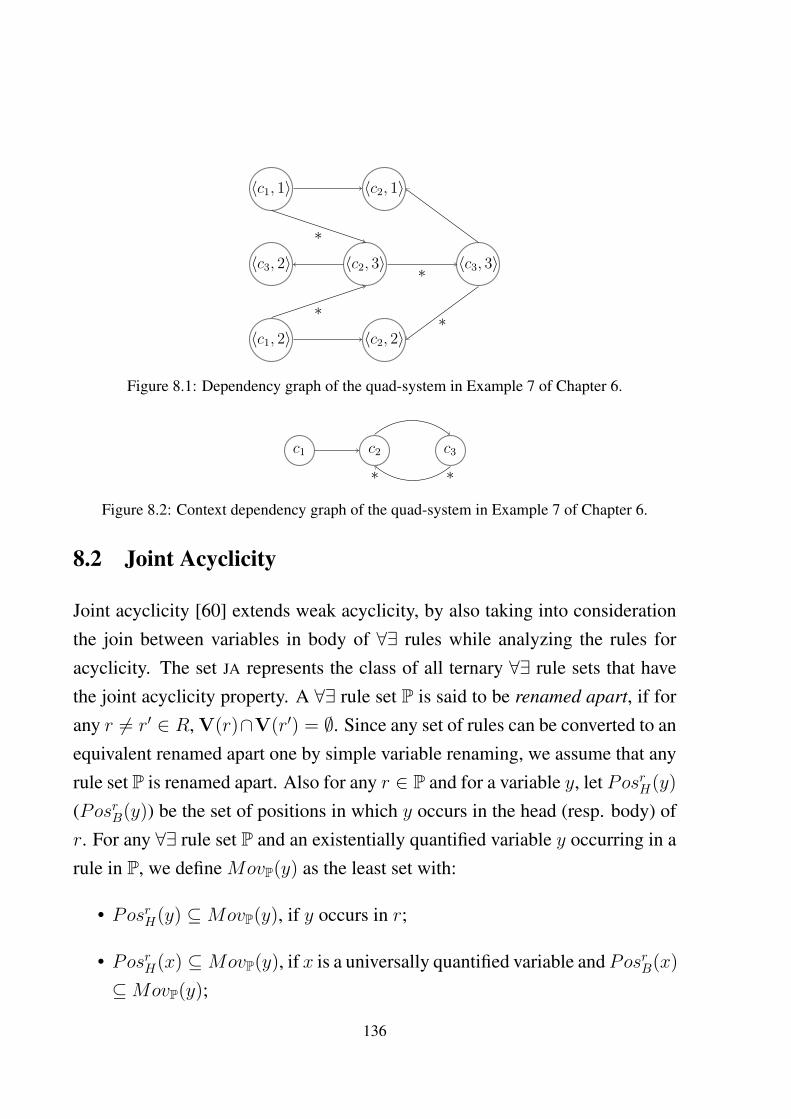
〈c1, 1〉

〈c1, 2〉

〈c2, 1〉

〈c2, 3〉

〈c2, 2〉

〈c3, 3〉〈c3, 2〉

∗

∗

∗

∗

Figure 8.1: Dependency graph of the quad-system in Example 7 of Chapter 6.

c1 c2

∗c3

∗

Figure 8.2: Context dependency graph of the quad-system in Example 7 of Chapter 6.

8.2 Joint Acyclicity

Joint acyclicity [60] extends weak acyclicity, by also taking into considerationthe join between variables in body of ∀∃ rules while analyzing the rules foracyclicity. The set JA represents the class of all ternary ∀∃ rule sets that havethe joint acyclicity property. A ∀∃ rule set P is said to be renamed apart, if forany r 6= r′ ∈ R, V(r)∩V(r′) = ∅. Since any set of rules can be converted to anequivalent renamed apart one by simple variable renaming, we assume that anyrule set P is renamed apart. Also for any r ∈ P and for a variable y, let PosrH(y)

(PosrB(y)) be the set of positions in which y occurs in the head (resp. body) ofr. For any ∀∃ rule set P and an existentially quantified variable y occurring in arule in P, we define MovP(y) as the least set with:

• PosrH(y) ⊆MovP(y), if y occurs in r;

• PosrH(x) ⊆MovP(y), if x is a universally quantified variable and PosrB(x)

⊆MovP(y);

136

for any r ∈ P. The existential dependency graph of a (renamed apart) set ofrules P is a graph whose nodes are the existentially quantified variables in P.There exists an edge from a variable y to y′, if there is a rule r ∈ P in whichy′ occurs and there exists a universally quantified variable x in the head (andbody) of r such that PosrB(x) ⊆MovP(y). A ∀∃ rule set P is jointly acyclic, iffits existential dependency graph is acyclic. Analyzing the containment relation-ships, it happens to be the case that JA 6⊆ CSAFE (since WA ⊂ JA, and eg. 10).Also example 11 shows us that CSAFE 6⊆ JA. However JA ⊂ MSAFE, since JA

⊂ MFA and MFA ≡ MSAFE (Theorem 12).

Example 11. Consider the quad-system QSC = 〈QC, R〉, where QC = {c1 : (a,b, c)}. Suppose R is the following set:

R =

c1 : (x11, x12, z1)→ c2 : (x11, x12, y1) (r1)

c1 : (x21, x22, z2), c2 : (x22, x21, x23)→ c3 : (x21, x22, x23) (r2)

c3 : (x31, x32, x33)→ c1 : (x33, x31, x32) (r3)

Iterations during the dChase construction are:

dChase0(QSC) = {c1:(a, b, c)}

dChase1(QSC) = {c1 : (a, b, c), c2 : (a, b, : b1)}

dChase(QSC) = dChase1(QSC)

Note that the lone Skolem blank node generated is : b1, which do not have anydescendants. Hence, by definition QSC is csafe (msafe/safe). Now analyzingthe BRs for joint acyclicity, we note that for the only existentially quantifiedvariable y1,MovR(y1) = {〈c2, 3〉, 〈c3, 3〉, 〈c1, 1〉}

Since the BR r1 in which y1 occurs contains the universally quantified variablex11 in head of r1 such that Posr1

B (x11) ⊆MovR(y1), there exists a cycle from y1

to y1 itself in the existential dependency graph of τ(QSC). Hence, by definitionτ(QSC) is not joint acyclic. Also since the class of weakly acyclic rules are

137

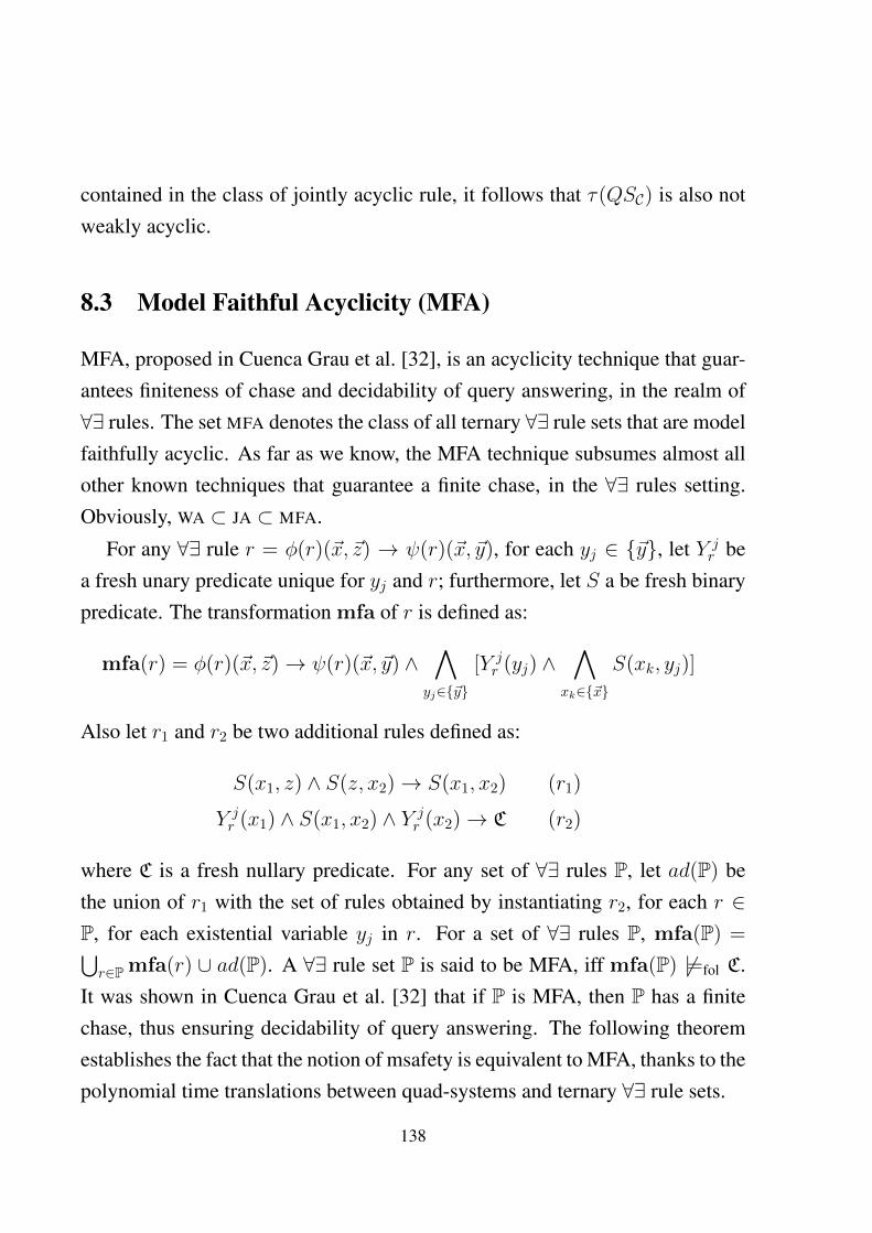
contained in the class of jointly acyclic rule, it follows that τ(QSC) is also notweakly acyclic.

8.3 Model Faithful Acyclicity (MFA)

MFA, proposed in Cuenca Grau et al. [32], is an acyclicity technique that guar-antees finiteness of chase and decidability of query answering, in the realm of∀∃ rules. The set MFA denotes the class of all ternary ∀∃ rule sets that are modelfaithfully acyclic. As far as we know, the MFA technique subsumes almost allother known techniques that guarantee a finite chase, in the ∀∃ rules setting.Obviously, WA ⊂ JA ⊂ MFA.

For any ∀∃ rule r = φ(r)(~x, ~z) → ψ(r)(~x, ~y), for each yj ∈ {~y}, let Y jr be

a fresh unary predicate unique for yj and r; furthermore, let S a be fresh binarypredicate. The transformation mfa of r is defined as:

mfa(r) = φ(r)(~x, ~z)→ ψ(r)(~x, ~y) ∧∧

yj∈{~y}

[Y jr (yj) ∧

∧xk∈{~x}

S(xk, yj)]

Also let r1 and r2 be two additional rules defined as:

S(x1, z) ∧ S(z, x2)→ S(x1, x2) (r1)

Y jr (x1) ∧ S(x1, x2) ∧ Y j

r (x2)→ C (r2)

where C is a fresh nullary predicate. For any set of ∀∃ rules P, let ad(P) bethe union of r1 with the set of rules obtained by instantiating r2, for each r ∈P, for each existential variable yj in r. For a set of ∀∃ rules P, mfa(P) =⋃r∈Pmfa(r) ∪ ad(P). A ∀∃ rule set P is said to be MFA, iff mfa(P) 6|=fol C.

It was shown in Cuenca Grau et al. [32] that if P is MFA, then P has a finitechase, thus ensuring decidability of query answering. The following theoremestablishes the fact that the notion of msafety is equivalent to MFA, thanks to thepolynomial time translations between quad-systems and ternary ∀∃ rule sets.

138

Theorem 12. Let τ be the translation function from the set of unrestricted quad-

systems to the set of ternary ∀∃ rule sets, as defined in Definition 1, then, for

any quad-system QSC = 〈QC , R〉, QSC is msafe iff τ(QSC) is MFA.

Proof. (outline) Recall that τ = 〈τq, τbr〉, where τq is the quad translation func-tion and τbr is the translation function from BRs to ∀∃ rules. Also, τ(QSC) =

τbr({rQC} ∪ R). Also, recall that for every blank node b in QC , the BR rQC

contains a corresponding existentially quantified variable yb. We already sawthat, for such a transformation, the following property holds: for any m ∈ N,τq(dChasem(QSC)) = chasem(τ(QSC)), and for any BR r ∈ R ∪ {rQC}, as-signment µ, applicableR∪{rQC}(r, µ, dChasem(QSC)) iff applicableτ(QSC)(τbr(r),µ, chasem(τ(QSC))). Also notice that for any two blank nodes : b1, : b2,S( : b1, : b2) ∈ chase(τ(QSC)), iff : b1 is a descendant of : b2 with respectto dChase(QSC). Hence, the relations S and descendantOf are identical.

Intuitively, MFA looks for cyclic creation of a Skolem blank-node whosedescendant is another Skolem blank-node that is generated by the same ruler = body(r)(~x, ~z) → head(r)(~x, ~y), by the same existential variable in yj ∈{~y} of r. Wheras, msafety looks only for generation of a Skolem blank-node: b′ whose descendant is another Skolem : b using the same rule r. Hence, ifτ(QSC) is not MFA, then QSC is not msafe, and consequently onlyIf part of thetheorem trivially holds.

(If part) Suppose QSC is unmsafe, and µ and µ′ are the assignments appliedon r ∈ R to create Skolem blank nodes : b and : b′, respectively, and suppose: b is a descendant of : b′ in the dChase(QSC). That is : b = µ(yj) and: b′ = µ′(yk), for yj, yk ∈ {~y} of r. Suppose j = k, then the prerequisite of

non-MFA is trivially satisfied. Suppose if j 6= k is the case, then there exists: b′′ in dChase(QSC) such that : b′′ = µ′(yj), since µ′ is applied on r andyj ∈ {~y}. This means that also in this case, the prerequisite of non-MFA issatisfied. As a consequence τ(QSC) is not MFA. Hence it follows that, QSC ismsafe iff τ(QSC) is MFA.

139

Let us revisit the quad-system QSC in Example 10 of Chapter 6, it can be easilyseen that τ(QSC) is not MFA. Recall that we have seen that QSC is safe but notmsafe. We consider the Theorem 12 to be of importance, as it not only estab-lishes the equivalence of MFA and msafety, but thanks to it and the translationτ , it can be deduced that the technique of safety, which we presented earlier,(strictly) extends the MFA technique. As far as we know, the MFA class of∀∃ rule sets is one of the most expressive class in the realm of ∀∃ rule setswhich allows a finite chase. Hence, the notion of safety that we propose canstraightforwardly be ported to ∀∃ settings. The main difference between MFAand safety is that MFA only looks for cyclic creation of two distinct Skolemblank-nodes : b, : b′ that are generated by the same rule r, by the same exis-tential variable in r. Whereas safety also takes into account the origin vectors~a and ~a′ used during rule application to create : b and : b′, respectively, andonly raises an alarm if ~a ∼= ~a′. Although, equivalence holds only between quad-systems and ternary ∀∃ rule sets, it can easily be noticed that the technique ofsafety can be applied to ∀∃ rule sets of arbitrary arity, and can be used to ex-tend currently established tools and systems that work on existing notions ofacyclicity such as WA, JA, or MFA.

140

Chapter 9

Related work

9.1 Contexts and Distributed Logics

Work on contexts gained its attention as early as in the 80s, as McCarthy [55]proposed context as a solution to the generality problem in AI. McCarthy inworks such as [55, 73] lists a few problems in his past efforts on formalizingcontexts, and proposed a general solution – represent contexts as first class ob-jects. After this, various studies about logics of contexts mainly in the fieldof KR were done by Guha [84], Distributed First Order Logics by Ghidini etal. [42] and Local Model Semantics by Giunchiglia et al. [41]. In his thesis [84],Guha implemented several of the existing ideas of McCarthy, and exemplfiedusing several realistic examples how context can be used to solve several reallife problems. Ghidini’s and Giunchiglia’s ideas were primarily grounded onthe “Context as a box” paradigm elaborated in Benerecetti et al. [71]. The“Context as a box” approach proposes the formalization of a context as a theoryplus a set of dimension-value pairs for a fixed set of contextual dimensions [36].Bao et.al. [8] extended the theory of McCarthy [74, 55] by providing a moreconcrete formalization using the built in predicate isin. A number of constructswere introduced for combining contexts (c1∧c2, c1∨c2 and ¬c) and for relatingcontexts (c1 ⇒ c2, and c1 → c2). Primarily in the above works, contexts wereformalized as a first order/propositional theory and bridge rules were provided

141

to inter-operate the various theories of contexts.

Some of the initial works on contexts relevant to SW were the ones like Dis-

tributed Description Logics (DDL) [14] by Borgida et al., Context-OWL [15] byBouquet et al., and the recent work of CKR [86, 75, 16] by Serafini and Bozzatoet al. These were mainly logics based on DLs, which formalized contexts asOWL KBs, whose semantics is given using a distributed interpretation structurewith additional semantic conditions that suits varying requirements. DDL andContext-OWL, provides a language for extending ontologies in DL/OWL withcontexts. Rather than a global/shared approach in which ontologies can exter-nally refer to other ontologies via import statement, the contextualized/localizedapproach in DDL/Context-OWL is to allow the co-existence of multiple local-ized OWL/DL theories, called contexts. A limited or controlled form of glob-alization is possible by the virtue of mappings via bridge rules. Mappings areprojections of local domain onto an external domain, and vice versa. The se-mantics using domain relations rij make it possible to have directional map-pings between a pair of contexts ci, cj, i.e. to have mappings from ci to cj thatdiffer from the mappings from cj to ci. Also, Context-OWL/DDL defines themechanism of a hole, an interpretation in which every concept (resp. role) ismapped to the universal set (resp. relation), in order to prohibit propagation ofinconsistencies from a context to another via mappings. Different from DDLand Context-OWL, the CKR allows to formalize the relation of coverage be-tween contexts, that establishes the inclusion relationship of their correspondingdomains. Also, in order to refer to concept/role symbols in foreign context, aconcept/role symbol can be qualified with a context identifier. The CKR seman-tics specifies how the extension of a qualified concept/role in a context inheritsthe objects of the same from its covered/covering contexts. Euzenat in [38]describes the Tropes taxonomy building framework, that enables the concep-tualization of objects in multiple viewpoints (similar to our contexts), also thesupport for conjunctive bridges allows to map a set of concepts in viewpoints

142

to a concept in another viewpoint. Harth et al. in [49] describe a detailed ar-chitecture of Yars, a semantic repository with a search/query engine that storesRDF data in the form of ((s, p, o), c) where (s, p, o) is an RDF triple in contextc. The architecture contains modules that includes the crawler, index managerand indexer, query processing and a query distribution module. The indexingmodule contains an keyword based indexer and a quad index that is distributedover multiple servers that also includes a context identifier as an index key.Compared to these works, the bridge rules we consider are much more expres-sive with conjunctions and existential variables that supports value/blank-nodecreation. Also, none of the above works are focused on the query answeringproblem, which is the main focus of this thesis work.

9.2 Temporal/Annotated RDF

Studies in extending standard RDF with dimensions such as time and annota-tions have already been accomplished. Gutierrez et al. in [46] tried to add atemporal extension to RDF and defines the notion of a ‘temporal rdf graph’, inwhich a triple is augmented to a quadruple of the form t : (s, p, o), where t isa time point. Also, the authors extend the standard conjunctive graph querieswith a temporal query language that supports temporal variables. A semanticsis provided for interpreting temporal RDF graphs, from which the notion oftemporal entailment of graphs and queries follows. The authors also provide asound and complete set of inference rules, and show that entailment of temporalgraphs does not yield extra computational complexity than standard RDF graphentailment.

Annotated extensions to RDF and querying annotated graphs have been stud-ied in Udrea et al. [92], Straccia [89], and Zimmerman et al. [93]. Unlikethe case of time, here the quadruple has the form: a : (s, p, o), where a isan annotation. In Udrea et al. [92], the authors assume that the annotation a

143

in the triple a : (s, p, o) is a member of a strict partial order, whereas Strac-cia [89], and Zimmerman et al. assume that a is taken from an annotationdomain that is an idempotent, commutative semi-ring, with the addition opera-tion, +, being >-annihilating, i.e. x + > = >, for all x in the annotation do-main. The use of such a structure for the annotation domain, allows the authorsto infer [2000 − 2002] : (a, rdfs:subClassOf, c) from [1999 − 2002] : (a,rdfs:subClassOf, b) and [2000 − 2005] : (b, rdfs:subClassOf, c),whereas Udrea et al. [92] do not support this type of inferencing. The authorsprovide semantics, inference rules/algorithms and a query language that allowsfor expressing temporal/annotated queries. While Udrea et al. [92] only sup-ports conjunctive type queries, Zimmerman et al. [93] supports full SPARQL1.0 and many features of SPARQL 1.1 such as grouping, ordering, nested queries,variable assignments, and built-in predicates on the annotation domain. The au-thors call their extended query language, AnQL. Also, the authors in [93] showhow their framework is suited for concrete real world cases, by illustrating howconcrete dimensions such as time, fuzziness, and provenance satisfy the prop-erties of an annotation domain, and exemplifies the applications of their frame-work on these domains. The authors also demonstrate the suitability of theirframework for RDF statements that have annotation from different domains (forinstance, time and fuzziness), and also show how AnQL querying can be doneon the combination of annotated and non-annotated data. Although these ap-proaches, in a way, address contexts by means of time and annotations, themain difference in our work is that we provide the means to specify expressivebridge rules for inter-operating the reasoning between the various contexts.

9.3 Description Logic Rules

Works on extending DL KBs with Datalog like rules was studied by Grosofet al. [13]. The authors in [13], propose a fragment of DL, called descrip-

144

tion horn logic (DHL), contained within the intersection of DLs and logic pro-grams [33]. The authors define a translation mechanism for translating an ar-bitrary DHL ontology to a function-free positive Horn logic program, and il-lustrate how the common reasoning DL problems such as instance checkingover classes/roles, subsumption checking/satisfiability of classes/roles can bereduced to atom entailment in logic programming. Related initiatives gave riseto SWRL[54], which is a formalism using which one can mix a DL ontologywith the Unary/Binary Datalog RuleML sublanguages of the Rule Markup Lan-guage, and hence enables Horn-like rules to be combined with an OWL KB.Since SWRL is undecidable in general, studies on computable sub-fragmentsgave rise to works like Description Logic Rules [62] and its extensions [29],where the authors deal with rules that can be totally internalized by a DL knowl-edge base, and hence if the DL considered is decidable, then also is a DL+rulesKB. The authors give various fragments of the rule bases like SROIQ rules,EL++ rules etc. and show that certain new constructs that are not expressible byplain DL can be expressed using rules although they are finally internalized intoDL KBs. Unlike in our scenario, these works consider only horn rules withoutexistential variables.

9.4 ∀∃ rules, Tuple Generating Dependencies, Datalog+- rules

Query answering over rules with universal-existential quantifiers in the contextof databases, where these rules are called Datalog+- rules/tuple generating de-pendencies (TGDs), was done by Beeri and Vardi [12] even in the early 80s,where the authors show that the query entailment problem, in general, is un-decidable. However, recently many classes of such rules have been identifiedfor which query answering is decidable. These classes (according to [6]) canbroadly be divided into the following three categories: (i) bounded treewidth

sets (BTS), (ii) finite unification sets (FUS), and (iii) finite extension sets (FES).

145

BTS contains the classes of ∀∃ rule sets, whose models have bounded treewidth.Some of the important classes of these sets are the linear ∀∃ rules [56], (weakly)guarded rules [21], (weakly) frontier guarded rules [6], and jointly frontierguarded rules [60]. BTS classes in general need not have a finite chase, andquery answering is done by exploiting the fact that the chase is tree shaped,whose nodes (which are sets of instances) start replicating (up to isomorphism)after a while. Hence, one could stop the computation of the chase, once it canbe made sure that any future iterations of chase can only produce nodes thatare isomorphic to existing nodes. A deterministic algorithm for deciding queryentailment for this class is provided in Thomazo et al. [91].

FUS classes include the class of ‘sticky’ rules [23, 22], atomic hypothesisrules in which the body of each rule contains only a single atom, and also theclass of linear ∀∃ rules. The approach used for query answering in FUS classesis to rewrite the input query w.r.t. to the ∀∃ rule sets to another query that canbe evaluated directly on the set of instances, s.t. the answers for the formerquery and latter query coincides. The approach is called the query rewriting ap-

proach. Compared to approaches proposed in this dissertation, these approachesdo not enjoy the finite chase property, and are hence not conducive to material-ization/forward chaining based query answering.

Unlike BTS and FUS, the FES classes are characterized by the finite chaseproperty, and hence are most related to the techniques proposed in our work.Some of the classes in this set employ termination guarantying checks called‘acyclicity tests’ that analyze the information flow between rules to check whethercyclic dependencies exists that can lead to infinite chase. Weak acyclicity [39,34], was one of the first such notions, and was extended to joint acyclicity [60]and super weak acyclicity [69]. The main approach used in these techniques isto exploit the structure of the rules and use a dependency graph that models thepropagation path of constants across various predicates in the rules, and restrict-ing the dependency graph to be acyclic. The main drawback of these approaches

146

is that they only analyze the schema/Tbox part of the rule sets, and ignore theinstance part, and hence produce a large number of false alarms, i.e. it is oftenthe case that although dependency graph is cyclic, the chase is finite. Recently,a more dynamic approach, called the MFA technique, that also takes into ac-count the instance part of the rule sets was proposed in Cuenca grau et al. [32],where existence of cyclic Skolem blank-node/constant generations in the chaseis detected by augmenting the rules with extra information that keeps track ofthe Skolem function used to generate each Skolem blank-node. As shown inChapter 8, our technique of safety subsumes the MFA technique, and supportsfor much more expressive rule sets, by also keeping track of the vectors used byrule bodies while Skolem blank-nodes are generated.

9.5 Data integration

Studies in query answering on integrated heterogeneous databases with expres-sive integration rules in the realm of data integration is primarily studied in thefollowing two settings: (i) Data exchange [39], in which there is typically asource database and target database that are connected with existential rules,and (ii) Peer-to-peer data management systems (PDMS) [47], where there arean arbitrary number of peers that are interconnected using existential rules.

It can be noted that the peer-to-peer extension of (i) given in works such as[40, 2] has a similar architecture as (ii). The variant of data exchange problemin the realm of SW, called the P2P RDF Data Exchange setting, as presented inBarcelo et al. [10] is a system of RDF graphs interconnected using ∀∃ rules. Auser query is typically a conjunctive query on any of the peers. The answer tothe query is computed taking into account not only the knowledge in the peer,but also the mappings to the other peers. The approach based on dependencygraphs, for instance, is used by Halevi et al. in the context of peer-peer datamanagement systems [47], and decidability is attained by not allowing any kind

147

of cycles in the peer topology. Whereas in the context of Data exchange, WA isused in [39, 34] to assure decidability, and the recent work by Marnette [69] em-ploys the super weak acyclicity (SWA) to ensure decidability. It was shown inCuenca Grau et al [32] that their MFA technique strictly subsumes both WA andSWA techniques in expressivity. Since we saw in Chapter 8 that our techniqueof safety subsumes the MFA technique and allows the representation of muchmore expressive rule sets, the safety technique can straightforwardly be em-ployed in the above mentioned systems with decidability guarantees for queryanswering.

9.6 Distributed/Federated SPARQL Querying

Support for SPARQL queries that span multiple graphs/datasets was alreadyprovided in SPARQL 1.0 [83] via FROM, FROM NAMED, and the GRAPHkeywords. This has been extended to SPARQL querying over federated datasources/graphs by Buil-Aranda et al [19] and SPARQL 1.1, where the authorsintroduce multiple constructs for SPARQL queries that span multiple endpoints,and gives an extension of the SPARQL algebra for the federated extension.Chekol in his PhD thesis [31] studied the containment of SPARQL 1.1 queriesin the presence of constraints expressed in RDFS and OWL-ALCH. Chekol re-duces the containment problem of SPARQL queries to the validity problem inµ-calculus by translating both queries and constraints to formulas in µ-calculus.Though these query languages are similar in a way to the CCQs that span multi-ple contexts, the main difference is the presence of expressive forall-existentialBRs in our work that can potentially cause non-termination. Also different fromthe above works, in our thesis work, we derive novel classes for which CCQ an-swering is decidable.

148

Chapter 10

Summary and Conclusion

In this thesis, we study the problem of query answering over contextualizedRDF knowledge in the presence of forall-existential bridge rules. We show thatthe problem, in general, is undecidable, and present a number of decidable sub-classes of quad-systems. Table 10.1 displays the complexity results of chasecomputation and query entailment for the various classes of quad-systems wehave derived. Fig. 10.1 graphically portrays the landscape of decidable classesthat we derived in this thesis work, along with the already existing classes in the∀∃ rules paradigm, namely the classes of model faithful acyclic rulesets (MFA),jointly acyclic rulesets (JA), and weakly acyclic rulesets (WA). There is a bidi-rectional edge between two nodes in the graph if there is an equivalence relationbetween classes represented by these nodes. Hence, there is a bidirectional edgebetween UNRESTRICTED QUAD-SYSTEMS and TERNARY ∀∃ RULES classes,and also a bidirectional edge between MSAFE and MFA. Also, note that a unidi-rectional edge/path exists between a node to another, if the class represented bythe former is contained in the class represented by the latter, and in case if thelatter is at a higher altitude then it signifies strict containment.

The class of context acyclic quad-systems do not allow cyclic dependenciesinvolving triple generating contexts. Classes csafe, msafe, and safe, ensure de-cidability by restricting the structure of Skolem blank-nodes generated in the

149

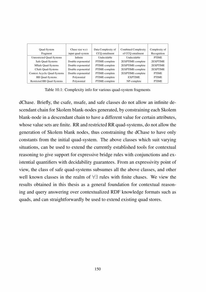
Quad-System Chase size w.r.t Data Complexity of Combined Complexity Complexity ofFragment input quad-system CCQ entailment of CCQ entailment Recognition

Unrestricted Quad-Systems Infinite Undecidable Undecidable PTIMESafe Quad-Systems Double exponential PTIME-complete 2EXPTIME-complete 2EXPTIME

MSafe Quad-Systems Double exponential PTIME-complete 2EXPTIME-complete 2EXPTIMECSafe Quad-Systems Double exponential PTIME-complete 2EXPTIME-complete 2EXPTIME

Context Acyclic Quad-Systems Double exponential PTIME-complete 2EXPTIME-complete PTIMERR Quad-Systems Polynomial PTIME-complete EXPTIME PTIME

Restricted RR Quad-Systems Polynomial PTIME-complete NP-complete PTIME

Table 10.1: Complexity info for various quad-system fragments

dChase. Briefly, the csafe, msafe, and safe classes do not allow an infinite de-scendant chain for Skolem blank-nodes generated, by constraining each Skolemblank-node in a descendant chain to have a different value for certain attributes,whose value sets are finite. RR and restricted RR quad-systems, do not allow thegeneration of Skolem blank nodes, thus constraining the dChase to have onlyconstants from the initial quad-system. The above classes which suit varyingsituations, can be used to extend the currently established tools for contextualreasoning to give support for expressive bridge rules with conjunctions and ex-istential quantifiers with decidability guarantees. From an expressivity point ofview, the class of safe quad-systems subsumes all the above classes, and otherwell known classes in the realm of ∀∃ rules with finite chases. We view theresults obtained in this thesis as a general foundation for contextual reason-ing and query answering over contextualized RDF knowledge formats such asquads, and can straightforwardly be used to extend existing quad stores.

150

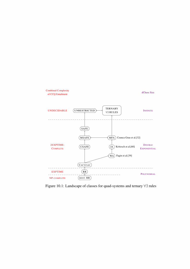
Combined Complexityof CCQ Entailment

dChase Size

UNRESTRICTEDUNDECIDABLE INFINITETERNARY∀∃ RULES

SAFE

MSAFE MFA Ceunca Grau et al.[32]

CSAFE JA Krotzsch et al.[60]

WA Fagin et al.[39]

CACYCLIC

2EXPTIME-COMPLETE

DOUBLE

EXPONENTIAL

RREXPTIMEPOLYNOMIAL

REST. RRNP-COMPLETE

Figure 10.1: Landscape of classes for quad-systems and ternary ∀∃ rules

Bibliography

[1] Abiteboul, S., Hull, R., Vianu, V.: Foundations of Databases. Addison-Wesley (1995)

[2] Arenas, M., Barcelo, P., Libkin, L., Murlak, F.: Relational andXML Data Exchange. Synthesis Lectures on Data Management, Mor-gan & Claypool Publishers (2010), http://dx.doi.org/10.2200/S00297ED1V01Y201008DTM008

[3] Arora, S., Barak, B.: Computational Complexity: A Modern Approach.Cambridge University Press, New York, NY, USA, 1st edn. (2009)

[4] Baader, F., Brandt, S., Lutz, C.: Pushing the EL envelope. In: Proceedingsof the 19th International Joint Conference on Artificial Intelligence IJCAI-05. Edinburgh, UK (2005)

[5] Baader, F., Calvanese, D., McGuinness, D.L., Nardi, D., Patel-Schneider,P.F. (eds.): The Description Logic Handbook: Theory, Implementation,and Applications. Cambridge University Press (2003)

[6] Baget, J.F., Leclere, M., Mugnier, M.L., Salvat, E.: On rules with existen-tial variables: Walking the decidability line. Artificial Intelligence 175(9-10), 1620–1654 (2011)

[7] Baget, J.F., Mugnier, M.L., Rudolph, S., Thomazo, M.: Walking the Com-plexity Lines for Generalized Guarded Existential Rules. In: IJCAI. pp.712–717 (2011)

153

[8] Bao, J., Tao, J., McGuinness, D.: Context Representation for the SemanticWeb. In: In Proceedings of the Web Science Conference 2010. Online athttp://www.websci10.org/ (2010)

[9] Bao, J., Voutsadakis, G., Slutzki, G., Honavar, V.: Package-based descrip-tion logics. In: Modular Ontologies, pp. 349–371 (2009)

[10] Barcelo, P., Perez, J., Reutter, J.: Schema Mappings and Data Exchangefor Graph Databases. In: Proceedings of the 16th International Conferenceon Database Theory. pp. 189–200. ICDT ’13, ACM, New York, NY, USA(2013), http://doi.acm.org/10.1145/2448496.2448520

[11] Bechhofer, S., van Harmelen, F., Hendler, J., Horrocks, I., McGuinness,D.L., Patel-Schneider, P.F., Stein, L.A.: OWL Web Ontology LanguageReference. Tech. rep., W3C, http://www.w3.org/TR/owl-ref/ (February2004)

[12] Beeri, C., Vardi, M.Y.: The Implication Problem for Data Dependencies.In: ICALP. pp. 73–85 (1981)

[13] Benjamin N. Grosof, Ian Horrocks, R.V.S.D.: Description logic programs:Combining logic programs with description logic. In: Gusztav Hencseyand Bebo White Editors, Proceedings of the Twelfth International WorldWide Web Conference (WWW). pp. 48–57. ACM (2003)

[14] Borgida, A., Serafini, L.: Distributed Description Logics: AssimilatingInformation from Peer Sources. J. Data Semantics 1, 153–184 (2003)

[15] Bouquet, P., Giunchiglia, F., van Harmelen, F., Serafini, L., Stucken-schmidt, H.: C-owl: Contextualizing ontologies. In: ISWC. pp. 164–179(2003)

154

[16] Bozzato, L., Eiter, T., Serafini, L.: Defeasibility in Contextual Reasoningwith CKR. In: Italian Conference in Computation Logic (CILC). pp. 132–146 (2014)

[17] Bozzato, L., Ghidini, C., Serafini, L.: Comparing contextual and flat rep-resentations of knowledge: A concrete case about football data. In: Pro-ceedings of the seventh international conference on Knowledge capture(K-CAP ’13), 9-16, ACM 2013

[18] Brachman, R.J., Levesque, H.J.: Knowledge Representationand Reasoning. Elsevier - Morgan Kaufmann (2004), http:

//www.elsevier.com/wps/find/bookdescription.cws_

home/702602/description

[19] Buil-Aranda, C., Arenas, M., Corcho, O., Polleres, A.: Federating queriesin sparql 1.1: Syntax, semantics and evaluation. Web Semant. 18(1), 1–17(Jan 2013), http://dx.doi.org/10.1016/j.websem.2012.

10.001

[20] Calı, A., Gottlob, G., Lukasiewicz, T., Marnette, B., Pieris, A.: Datalog+/-: A Family of Logical Knowledge Representation and Query Languagesfor New Applications. In: Logic in Computer Science (LICS), 2010 25thAnnual IEEE Symposium on. pp. 228 –242 (july 2010)

[21] Calı, A., Gottlob, G., Kifer, M.: Taming the Infinite Chase: Query Answer-ing under Expressive Relational Constraints. In: KR. pp. 70–80 (2008)

[22] Calı, A., Gottlob, G., Pieris, A.: Towards more expressive ontologylanguages: The query answering problem. In: in Artificial Intelligence,vol. 93, Elsevier. pp. 87–128 (2012)

[23] Calı, A., Gottlob, G., Pieris, A.: Query Answering under Non-guardedRules in Datalog+/-. In: RR. pp. 1–17 (2010)

155

[24] Calvanese, D.: Finite Model Reasoning in Description Logics. In: KR. pp.292–303 (1996)

[25] Calvanese, D., Damaggio, E., De Giacomo, G., Lenzerini, M., Rosati,R.: Semantic data integration in p2p systems. In: Aberer, K., Koubarakis,M., Kalogeraki, V. (eds.) Databases, Information Systems, and Peer-to-Peer Computing, Lecture Notes in Computer Science, vol. 2944, pp. 77–90. Springer Berlin Heidelberg (2004), http://dx.doi.org/10.1007/978-3-540-24629-9_7

[26] Calvanese, D., De Giacomo, G., Lembo, D., Lenzerini, M., Rosati,R., Ruzzi, M.: Using OWL in data integration. In: De Virgilio, R.,Giunchiglia, F., Tanca, L. (eds.) Semantic Web Information Management –a Model Based Perspective, chap. 17, pp. 397–424. Springer Verlag (2009)

[27] Calvanese, D., Giacomo, G., Lembo, D., Lenzerini, M., Rosati, R.:Tractable Reasoning and Efficient Query Answering in Description Log-ics: The DL-Lite Family. J. Autom. Reason. 39(3), 385–429 (Oct 2007),http://dx.doi.org/10.1007/s10817-007-9078-x

[28] Carothers, G.: RDF 1.1 N-Quads. Tech. rep., W3C Recommendation(February 2014), http://www.w3.org/TR/n-quads/

[29] Carral Martnez, D., Hitzler, P.: Extending description logic rules. In:Simperl, E., Cimiano, P., Polleres, A., Corcho, O., Presutti, V. (eds.)The Semantic Web: Research and Applications, Lecture Notes in Com-puter Science, vol. 7295, pp. 345–359. Springer Berlin Heidelberg (2012),http://dx.doi.org/10.1007/978-3-642-30284-8_30

[30] Carroll, J., Bizer, C., Hayes, P., Stickler, P.: Named graphs, provenanceand trust. In: Proc. of the 14th int.l. conf. on WWW. pp. 613–622. ACM,New York, NY, USA (2005)

156

[31] Chekol, M.W.: Static analysis of semantic web queries. Ph.D.thesis (2012), ftp://ftp.inrialpes.fr/pub/exmo/thesis/thesis-chekol.pdf

[32] Cuenca Grau, B., Horrocks, I., Krotzsch, M., Kupke, C., Magka, D.,Motik, B., Wang, Z.: Acyclicity Notions for Existential Rules and TheirApplication to Query Answering in Ontologies. In: Journal of ArtificialIntelligence Research (JAIR), vol. 47. pp. 741–808. AI Access Foundation(2013)

[33] Dantsin, E., Eiter, T., Gottlob, G., Voronkov, A.: Complexity andexpressive power of logic programming. Computing Surveys (CSUR33(3) (Sep 2001), http://portal.acm.org/citation.cfm?

id=502807.502810

[34] Deutsch, A., Tannen, V.: Reformulation of XML Queries and Constraints.In: In ICDT. pp. 225–241 (2003)

[35] Deutsch, A., Nash, A., Remmel, J.: The chase revisited. In: Proceed-ings of the twenty-seventh ACM SIGMOD-SIGACT-SIGART sympo-sium on Principles of database systems. pp. 149–158. PODS ’08, ACM,New York, NY, USA (2008), http://doi.acm.org/10.1145/

1376916.1376938

[36] D.Lenat: The Dimensions of Context Space. Tech. rep., CYCorp(1998), published online https://courses.csail.mit.edu/

6.803/pdf/lenat2.pdf

[37] Doan, A., Halevy, A.Y., Ives, Z.G.: Principles of Data Integration. MorganKaufmann (2012)

[38] Euzenat, J.: Brief overview of t-tree: The tropes taxonomy build-ing tool. Proc. 4th ASIS SIG/CR workshop on classification research

157

, Columbus (OH US), (rev. Philip Smith, Clare Beghtol, Raya Fidel,Barbara Kwasnik (eds), Advances in classification research 4, Infor-mation today 4(1) (1994), http://journals.lib.washington.edu/index.php/acro/article/view/12612

[39] Fagin, R., Kolaitis, P.G., Miller, R.J., Popa, L.: Data Exchange: Semanticsand Query Answering. In: Theoretical Computer Science. pp. 28(1):89–124 (2005)

[40] Fuxman, A., Kolaitis, P.G., Miller, R.J., Tan, W.C.: Peer Data Exchange.ACM Trans. Database Syst. 31(4), 1454–1498 (Dec 2006), http://doi.acm.org/10.1145/1189769.1189778

[41] Ghidini, C., Giunchiglia, F.: Local Models Semantics, or Contextual Rea-soning = Locality + Compatibility. Artificial Intelligence 127 (2001)

[42] Ghidini, C., Serafini, L.: Distributed first order logics. In: Frontiers OfCombining Systems 2, Studies in Logic and Computation. pp. 121–140.Research Studies Press (1998)

[43] Glimm, B., Lutz, C., Horrocks, I., Sattler, U.: Answering conjunctivequeries in the SHIQ description logic. In: Proceedings of the IJCAI’07.pp. 299–404. AAAI Press (2007)

[44] Goldreich, O.: Computational Complexity: A Conceptual Perspective.Cambridge University Press, New York, NY, USA, 1 edn. (2008)

[45] Guha, R., Mccool, R., Fikes, R.: Contexts for the semantic web. In: ISWC,volume 3298 of Lecture Notes in Computer Science. pp. 32–46. Springer(2004)

[46] Gutierrez, C., Hurtado, C.A., Vaisman, A.A.: Temporal RDF. In: ESWC.pp. 93–107 (2005)

158

[47] Halevy, A.Y., Ives, Z.G., Suciu, D., Tatarinov, I.: Schema Mediation inPeer Data Management Systems. In: In ICDE. pp. 505–516 (2003)

[48] Harrison, M.A.: Introduction to Formal Language Theory. Addison-Wesley Longman Publishing Co., Inc., Boston, MA, USA, 1st edn. (1978)

[49] Harth, A., Umbrich, J., Hogan, A., Decker, S.: YARS2: A federated repos-itory for querying graph structured data from the web. In: Proceedings ofthe ISWC/ASWC-2007 (2007)

[50] Hayes, P. (ed.): RDF Semantics. W3C Recommendation (Feb 2004),http://www.w3.org/TR/rdf-mt/

[51] Hitzler, P., Krotzsch, M., Parsia, B., Patel-Schneider, P.F., Rudolph, S.:OWL 2 Web Ontology Language Primer. W3C Recommendation, WorldWide Web Consortium (October 2009), http://www.w3.org/TR/owl2-primer/

[52] Homola, M., Serafini, L.: Augmenting Subsumption propogation in dis-tributed description logics. Applied Artificial Intelligence 24, 137–174(2010)

[53] Horrocks, I., Kutz, O., Sattler, U.: The Even More Irresistible SROIQ.In: Doherty, P., Mylopoulos, J., Welty, C.A. (eds.) KR. pp. 57–67. AAAI Press (2006), http://dblp.uni-trier.de/db/conf/kr/kr2006.html#HorrocksKS06

[54] Horrocks, I., Patel-Schneider, P.F., Boley, H., Tabet, S., Grosof, B., Dean,M.: SWRL: A Semantic Web Rule Language Combining OWL andRuleML. W3c member submission, World Wide Web Consortium (2004),http://www.w3.org/Submission/SWRL

[55] J.McCarthy: Generality in AI. Comm. of the ACM 30(12), 1029–1035(1987)

159

[56] Johnson, D.S., Klug, A.C.: Testing Containment of Conjunctive Queriesunder Functional and Inclusion Dependencies. J. Comput. Syst. Sci. 28(1),167–189 (1984)

[57] Joseph, M., Kuper, G., Serafini, L.: Query Answering over Contextual-ized RDF knowledge with Forall-Existential Bridge rules: Attaining De-cidability using Acyclicity. In: Italian Conference in Computation Logic(CILC-2014), Turin, Italy. pp. 210–224 (2014)

[58] Joseph, M., Kuper, G., Serafini, L.: Query Answering over ContextualizedRDF/OWL knowledge with Forall-Existential Bridge rules: Attaining De-cidability using Acyclicity. In: International Conference in Web Reasoningand Rule Systems (RR-2014), Athens, Greece (2014)

[59] Klarman, S., Gutierrez-Basulto, V.: Two-dimensional description logicsfor context-based semantic interoperability. In: Proceedings of AAAI-11(2011)

[60] Krotzsch, M., Rudolph, S.: Extending decidable existential rules by join-ing acyclicity and guardedness. In: Walsh, T. (ed.) Proceedings of the 22ndInternational Joint Conference on Artificial Intelligence (IJCAI’11). pp.963–968. AAAI Press/IJCAI (2011)

[61] Krotzsch, M.: The not-so-easy task of computing class subsumptions inOWL RL. In: Proceedings of the 11th International Semantic Web Con-ference. LNCS, Springer (2012)

[62] Krotzsch, M., Rudolph, S., Hitzler, P.: Description Logic Rules. In:Proceedings of the 18th European Conference on Artificial Intelligence(ECAI’08). pp. 80–84. IOS Press (2008)

160

[63] Krotzsch, M., Rudolph, S., Hitzler, P.: Complexities of horn descriptionlogics. ACM Trans. Comput. Log. 14(1), 2 (2013), http://doi.acm.org/10.1145/2422085.2422087

[64] Kutz, O., Lutz, C., Wolter, F., Zakharyaschev, M.: E-connections of ab-stract description systems. Artificial Intelligence 156(1), 1–73 (2004)

[65] Lenzerini, M.: Data integration: A theoretical perspective. In: Pro-ceedings of the Twenty-first ACM SIGMOD-SIGACT-SIGART Sympo-sium on Principles of Database Systems. pp. 233–246. PODS ’02, ACM,New York, NY, USA (2002), http://doi.acm.org/10.1145/

543613.543644

[66] Leone, N., Manna, M., Terracina, G., Veltri, P.: Efficiently ComputableDatalog Programs. International Conference in Knowledge Representationand Reasoning (KR 2012) (2012), http://www.aaai.org/ocs/index.php/KR/KR12/paper/view/4521

[67] L.Serafini, P.Bouquet: Comparing Formal Theories of Context in AI. Ar-tificial Intelligence 155, 41–67 (2004)

[68] Lutz, C., Toman, D., Wolter, F.: Conjunctive Query Answering in the De-scription Logic EL using a Relational Database System. In: Proceedingsof the 21st International Joint Conference on Artificial Intelligence (IJ-CAI09). AAAI Press (2009)

[69] Marnette, B.: Generalized Schema-Mappings: From Termination toTractability. In: Proceedings of the twenty-eighth ACM SIGMOD-SIGACT-SIGART Symposium on Principles of Database Systems. pp. 13–22. PODS ’09, ACM, New York, NY, USA (2009)

[70] Marnette, B., Geerts, F.: Static analysis of schema-mappings ensur-ing oblivious termination. In: Segoufin, L. (ed.) ICDT. pp. 183–195.

161

ACM International Conference Proceeding Series, ACM (2010),http://dblp.uni-trier.de/db/conf/icdt/icdt2010.

html#MarnetteG10

[71] M.Benerecetti, Bouquet, P., C.Ghidini: On the Dimensions of Context De-pendence. In: P.Bouquet, L.Serafini, R.H.Thomason (eds.) Perspectives onContexts, chap. 1, pp. 1–18. CSLI Lecture Notes, Center for the Study ofLanguage and Information/SRI (2007)

[72] M.Benerecetti, P.Bouquet, C.Ghidini: Contextual Reasoning Distilled. Ex-perimental and Theoretical AI 12(3), 279–305 (2000)

[73] Mccarthy, J.: A logical AI approach to context (1996), publishedonline http://www-formal.stanford.edu/jmc/logical/

logical.html

[74] McCarthy, J., Buvac, S., Costello, T., Fikes, R., Genesereth, M.,Giunchiglia, F.: Formalizing context (Expanded Notes) (1995)

[75] M.Joseph, L.Serafini: Simple reasoning for contextualized RDF knowl-edge. In: Proc. of Workshop on Modular Ontologies (WOMO-2011)(2011)

[76] Motik, B., Grau, B.C., Horrocks, I., Wu, Z., Fokoue, A., Lutz, C.: OWL 2Web Ontology Language – Profiles. Tech. rep., W3C (2009)

[77] Mylopoulos, J., Borgida, A., Jarke, M., Koubarakis, M.: Telos: Rep-resenting knowledge about information systems. Information Systems8(4), 325–362 (1990), http://www.cs.toronto.edu/˜nernst/papers/mylo-telos.pdf

[78] Parsia, B., Grau, B.C.: Generalized Link Properties for Expressiveepsilon-Connections of Description Logics. In: Veloso, M.M., Kambham-pati, S. (eds.) AAAI. pp. 657–662. AAAI Press / The MIT Press (2005)

162

[79] Patel-Schneider, P.F., Hayes, P., Horrocks, I.: OWL Web Ontol-ogy Language Semantics and Abstract Syntax Section 5. RDF-Compatible Model-Theoretic Semantics. Tech. rep., W3C (Dec 2004),http://www.w3.org/TR/owl-semantics/rdfs.html\

#built\_in\_vocabulary

[80] Patel-Schneider, P.F., Motik, B.: OWL 2 Web Ontology Language: Map-ping to RDF Graphs. World Wide Web Consortium, Working Draft WD-owl2-mapping-to-rdf-20081202 (December 2008)

[81] P.Bouquet, L.Serafini, H.Stoermer: Introducing Context into RDF Knowl-edge Bases. In: Proceedings the 2nd Italian Semantic Web Workshop(SWAP-2005). pp. 14–16 (2005)

[82] Perez, J., Arenas, M., Gutierrez, C.: Semantics and complexity of sparql.ACM Trans. Database Syst. 34, 16:1–16:45 (September 2009), http://doi.acm.org/10.1145/1567274.1567278

[83] Prud’hommeaux, E., Seaborne, A.: Sparql query language for rdf.W3c recommendation, W3C (Jan 2008), http://www.w3.org/TR/rdf-sparql-query/

[84] R.Guha: Contexts: a Formalization and some Applications. Ph.D. thesis,Stanford (1992)

[85] Schueler, B., Sizov, S., Staab, S., Tran, D.T.: Querying for meta knowl-edge. In: WWW ’08: Proceeding of the 17th international conferenceon World Wide Web. pp. 625–634. ACM, New York, NY, USA (2008),http://dx.doi.org/10.1145/1367497.1367582

[86] Serafini, L., Homola, M.: Contextualized Knowledge Repositories forthe Semantic Web. Web Semantics: Science, Services and Agents on the

163

World Wide Web (Special Issue on Reasoning with context in the SemanticWeb) (2012)

[87] Serafini, L., Tamilin, A.: DRAGO: Distributed Reasoning Architecture forthe Semantic Web. In: European Semantic Web Conference (ESWC). pp.361–376 (2005)

[88] Sirin, E., Parsia, B., Grau, B.C., Kalyanpur, A., Katz, Y.: Pellet: A Prac-tical OWL-DL Reasoner. Web Semant. 5(2), 51–53 (Jun 2007), http://dx.doi.org/10.1016/j.websem.2007.03.004

[89] Straccia, U., Lopes, N., Lukacsy, G., Polleres, A.: A general frame-work for representing and reasoning with annotated semantic web data.In: Proceedings of the 24th AAAI Conference on Artificial Intelli-gence (AAAI 2010), Special Track on Artificial Intelligence and theWeb (July 2010), http://www.polleres.net/publications/stra-etal-2010AAAI.pdf

[90] ter Horst, H.J.: Completeness, decidability and complexity of entail-ment for RDF Schema and a semantic extension involving the OWLvocabulary. Web Semantics: Science, Services and Agents on theWWW 3(2-3), 79–115 (2005), http://www.sciencedirect.

com/science/article/B758F-4H16P4Y-1/2/

d039e4784b224e95aafca856ecfb1edb, Selected Papers fromthe ISWC, 2004

[91] Thomazo, M., Baget, J.F., Mugnier, M.L., Rudolph, S.: A Generic Query-ing Algorithm for Greedy Sets of Existential Rules. In: KR’12: In-ternational Conference on Principles of Knowledge Representation andReasoning. pp. 096–106. Italie (2012), http://hal-lirmm.ccsd.cnrs.fr/lirmm-00763518

164

[92] Udrea, O., Recupero, D.R., Subrahmanian, V.S.: Annotated RDF. ACMTransactions on Computational Logic 11(2), 1–41 (2010)

[93] Zimmermann, A., Lopes, N., Polleres, A., Straccia, U.: A general frame-work for representing, reasoning and querying with annotated semanticweb data. Web Semantics 11, 72–95 (Mar 2012), http://dx.doi.org/10.1016/j.websem.2011.08.006

165

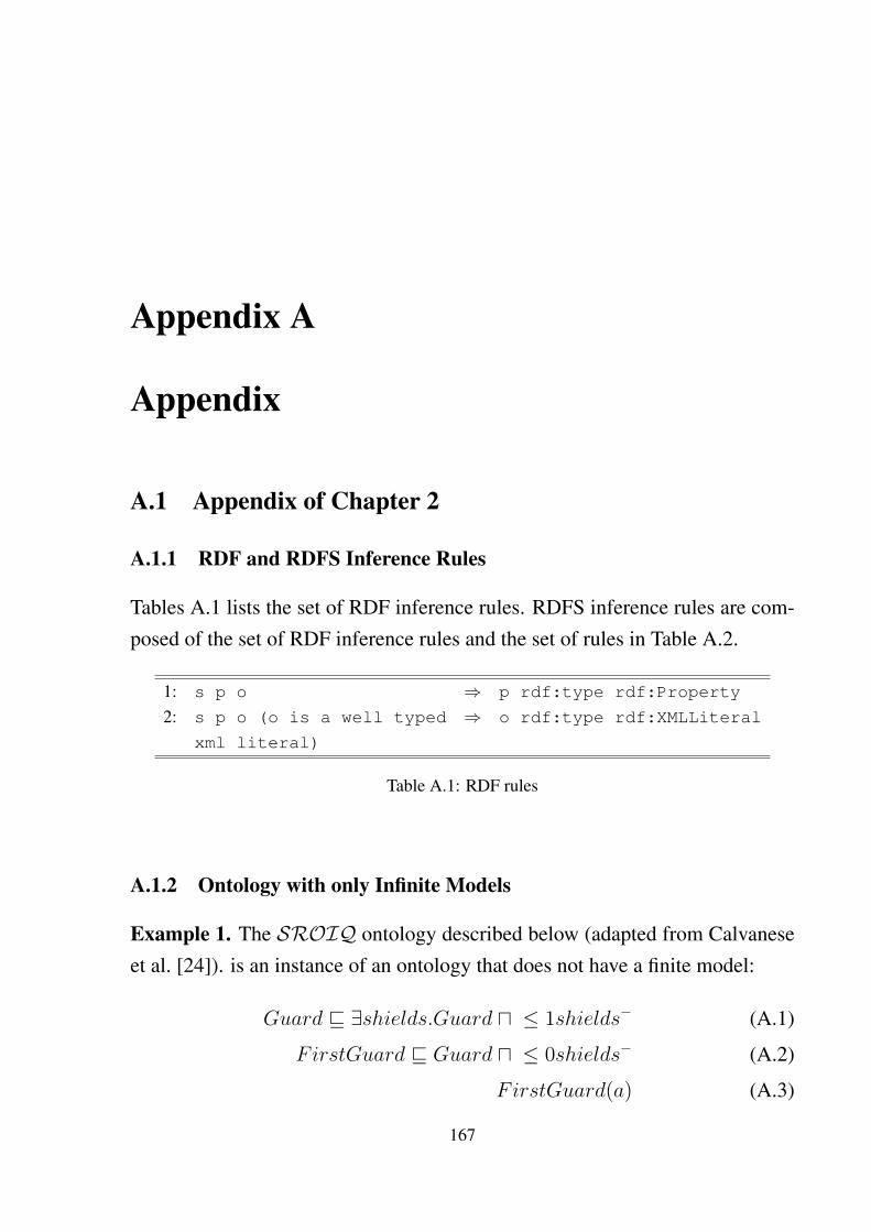
Appendix A

Appendix

A.1 Appendix of Chapter 2

A.1.1 RDF and RDFS Inference Rules

Tables A.1 lists the set of RDF inference rules. RDFS inference rules are com-posed of the set of RDF inference rules and the set of rules in Table A.2.

1: s p o ⇒ p rdf:type rdf:Property

2: s p o (o is a well typed ⇒ o rdf:type rdf:XMLLiteral

xml literal)

Table A.1: RDF rules

A.1.2 Ontology with only Infinite Models

Example 1. The SROIQ ontology described below (adapted from Calvaneseet al. [24]). is an instance of an ontology that does not have a finite model:

Guard v ∃shields.Guard u ≤ 1shields− (A.1)

FirstGuard v Guard u ≤ 0shields− (A.2)

FirstGuard(a) (A.3)

167

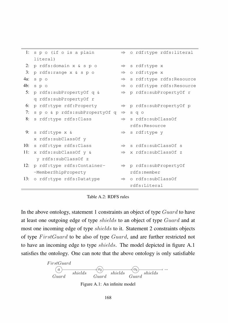
1: s p o (if o is a plain ⇒ o rdf:type rdfs:literal

literal)

2: p rdfs:domain x & s p o ⇒ s rdf:type x

3: p rdfs:range x & s p o ⇒ o rdf:type x

4a: s p o ⇒ s rdf:type rdfs:Resource

4b: s p o ⇒ o rdf:type rdfs:Resource

5: p rdfs:subPropertyOf q & ⇒ p rdfs:subPropertyOf r

q rdfs:subPropertyOf r

6: p rdf:type rdf:Property ⇒ p rdfs:subPropertyOf p

7: s p o & p rdfs:subPropertyOf q ⇒ s q o

8: s rdf:type rdfs:Class ⇒ s rdfs:subClassOf

rdfs:Resource

9: s rdf:type x & ⇒ s rdf:type y

x rdfs:subClassOf y

10: s rdf:type rdfs:Class ⇒ s rdfs:subClassOf s

11: x rdfs:subClassOf y & ⇒ x rdfs:subClassOf z

y rdfs:subClassOf z

12: p rdf:type rdfs:Container- ⇒ p rdfs:subPropertyOf

-MemberShipProperty rdfs:member

13: o rdf:type rdfs:Datatype ⇒ o rdfs:subClassOf

rdfs:Literal

Table A.2: RDFS rules

In the above ontology, statement 1 constraints an object of type Guard to haveat least one outgoing edge of type shields to an object of type Guard and atmost one incoming edge of type shields to it. Statement 2 constraints objectsof type FirstGuard to be also of type Guard, and are further restricted notto have an incoming edge to type shields. The model depicted in figure A.1satisfies the ontology. One can note that the above ontology is only satisfiable

a

Guard

F irstGuardo2

Guard

o3

Guard

...shields shields shields

Figure A.1: An infinite model

168

in models that have infinite domains, and is hence not finitely satisfiable. Theexample is a proof of existence of SROIQ ontologies that have only infinitesized models.


Proof of Property 1. Note that a strict linear order is a relation that is irreflexive,transitive, and linear.

Irreflexivity: By contradiction, suppose≺q is not irreflexive, then there existsQ ∈ Q such that Q ≺q Q holds. This means that neither of the conditions (i)and (ii) of ≺q definition holds for Q. Hence, due to condition (iii) Q 6≺q Q,which is a contradiction.

Linearity: Note that for any two distinct Q,Q′ ∈ Q, one of the followingholds: (a) Q ⊂ Q′, (b) Q′ ⊂ Q, or (c) Q \ Q′ and Q′ \ Q are non-empty anddisjoint. Suppose (a) is the case, then Q ≺q Q′ holds. Similarly, if (b) is thecase then Q′ ≺q Q holds. Otherwise if (c) is the case, then by condition (ii),either Q ≺q Q′ or Q′ ≺q Q should hold. Hence, ≺q is a linear order over Q.

Transitivity: Suppose there exists Q,Q′, Q′′ ∈ Q such that Q ≺q Q′ andQ′ ≺q Q′′. Then, one of the following four cases hold: (a) Q ≺q Q′ due to(i) and Q′ ≺q Q′′ due to (i), (b) Q ≺q Q′ due to (i) and Q′ ≺q Q′′ due to (ii),(c) Q ≺q Q′ due to (ii) and Q′ ≺q Q′′ due to (i), (d) Q ≺q Q′ due to (ii) andQ′ ≺q Q′′ due to (ii).

Suppose if (a) is the case, then trivially Q ⊂ Q′′, and hence by applying con-dition (i) Q ≺q Q′′. Otherwise if (b) is the case, then either (1) Q ⊂ Q′′ or (2)Q 6⊂ Q′′. Suppose, (1) is the case then, by (i) Q ≺q Q′′. Otherwise, if (2) is thecase, then since, Q ⊂ Q′, it cannot be the case that greatestQuad≺l

(Q′′ \Q) ≺lgreatestQuad≺l

(Q′′ \Q′), and it cannot be the case that greatestQuad≺l(Q′ \Q′′)

≺l greatestQuad≺l(Q\Q′′). Hence, it should be the case that greatestQuad≺l

(Q′′\Q′)�l greatestQuad≺l

(Q′′\Q) and greatestQuad≺l(Q\Q′′)≺l greatestQuad≺l

(Q′\

169

Q′′). But since, greatestQuad≺l(Q′ \Q′′)≺l greatestQuad≺l

(Q′′ \Q′), it followsthat greatestQuad≺l

(Q \ Q′′) ≺l greatestQuad≺l( Q′′ \ Q), and hence by con-

dition (ii), Q ≺q Q′′. Hence, if (b) is the case, then in both possible cases (1)or (2), it should be the case that Q ≺q Q′′. Otherwise if (c) is the case, thensimilar to the arguments in (b), by condition (i) or (ii), it can easily be seen thatQ ≺q Q′′.

Otherwise, if (d) is the case, then it must be the case that greatestQuad≺l(Q\

Q′)≺l greatestQuad≺l(Q′\Q) (†), and greatestQuad≺l

(Q′\Q′′)≺l greatestQua-d≺l

( Q′′ \Q′) (‡). Suppose by contradiction Q′′ ≺q Q, then one of the followingholds: (1) Q′′ ≺q Q by condition (i) or (2) Q′′ ≺q Q by condition (ii). Suppose,(1) is the case, then it should be the case that Q′′ ⊂ Q. Hence, it should not bethe case that greatestQuad≺l

( Q \Q′) ≺l greatestQuad≺l(Q′′ \Q′) and it should

not be the case that greatestQuad≺l(Q′\Q′′)≺l greatestQuad≺l

(Q′\Q). Hence,it should be the case that greatestQuad≺l

(Q′′ \ Q′) �l greatestQuad≺l(Q \ Q′)

(♥), and greatestQuad≺l( Q′ \ Q) �l greatestQuad≺l

(Q′ \ Q′′) (♠). Applying(‡) in (♥), we get greatestQuad≺l

(Q′ \ Q′′) ≺l greatestQuad≺l(Q \ Q′), and

applying (†) in (♠), we get greatestQuad≺l(Q\Q′)≺l greatestQuad≺l

(Q′\Q′′),which is a contradiction. Suppose if (2) is the case, then greatestQuad≺l

(Q′′ \Q) ≺l greatestQuad≺l

( Q \ Q′′). The last statement can also be written as:greatestQuad≺l

( Q′′ \ (Q ∩ Q′′)) ≺l greatestQuad≺l(Q \ (Q ∩ Q′′)). Using

Q ∩Q′ ∩Q′′ ⊆ Q ∩Q′, it follows that greatestQuad≺l(Q′′ \ (Q ∩Q′ ∩Q′′)) �l

greatestQuad≺l(Q\(Q∩Q′∩Q′′)) (♣). Also applying similar transformation in

(†) and (‡), we get greatestQuad≺l(Q \ (Q∩Q′∩Q′′))�l greatestQuad≺l

( Q′ \(Q∩Q′∩Q′′)), and greatestQuad≺l

(Q′\(Q∩Q′∩Q′′))�l greatestQuad≺l(Q′′\

(Q ∩ Q′ ∩ Q′′)). From which, it follows that greatestQuad≺l(Q \ (Q ∩ Q′ ∩

Q′′)) �l greatestQuad≺l(Q′′ \ (Q ∩ Q′ ∩ Q′′)). Using (♣) in the above, we get

greatestQuad≺l(Q \ (Q ∩Q′ ∩Q′′)) = greatestQuad≺l

(Q′ \ (Q ∩Q′ ∩Q′′)) =

greatestQuad≺l(Q′′ \ (Q∩Q′∩Q′′)), which is a contradiction. Hence, it should

be the case that Q ≺q Q′′.

170

Proof of Theorem 7. We show that the CCQ entailment problem is undecid-able for unrestricted quad-systems, by showing that the well known undecid-able problem of “non-emptiness of intersection of context-free grammars” isreducible to the CCQ entailment problem.

Given an alphabet Σ, string ~w is a sequence of symbols from Σ. A languageL is a subset of Σ∗, where Σ∗ is the set of all strings that can be constructed fromthe alphabet Σ, and also includes the empty string ε. Grammars are machineriesthat generate a particular language. A grammar G is a quadruple 〈V, T, S, P 〉,where V is the set of variables, T , the set of terminals, S ∈ V is the startsymbol, and P is a set of production rules (PR), in which each PR r ∈ P is ofthe form:

~w → ~w′

where ~w, ~w′ ∈ {T ∪ V }∗. Intuitively, application of a PR r of the form aboveon a string ~w1, replaces every occurrence of the sequence ~w in ~w1 with ~w′. PRsare applied starting from the start symbol S until it results in a string ~w, with~w ∈ Σ∗ or no more production rules can be applied on ~w. In the former case,we say that ~w ∈ L(G), the language generated by grammar G. For a detailedreview of grammars, we refer the reader to Harrison et al. [48]. A context-free

grammar (CFG) is a grammar, whose set of PRs P , have the following property:

Property 2. For a CFG, every PR is of the form v → ~w, where v ∈ V , ~w ∈{T ∪ V }∗.

Given two CFGs, G1 = 〈V1, T, S1, P1〉 and G2 = 〈V2, T, S2, P2〉, whereV1, V2, with V1 ∩ V2 = ∅, are the set of variables, T , such that T ∩ (V1 ∪ V2) =

∅, is the set of terminals. S1 ∈ V1 is the start symbol of G1, and P1 are the setof PRs of the form v → ~w, where v ∈ V , ~w is a sequence of the form w1...wn,where wi ∈ V1∪T . Similarly s2, P2 is defined. Deciding whether the languagesgenerated by the grammars L(G1) and L(G2) have a non-empty intersection isknown to be undecidable [48]. Since we can turing reduce the above problem

171

to the problem of non-emptiness checking of languages generated by two CFGsG′1 and G′2 s.t. ε 6∈ L(G′1) ∪ L(G′2), w.l.o.g we assume that both L(G1) andL(G2) does not contain the empty string ε.

Given two CFGs, G1 = 〈V1, T, S1, P1〉 and G2 = 〈V2, T, S2, P2〉, we encodegrammars G1, G2 into a quad-system of the form QSc = 〈Qc, R〉, with a singlecontext identifier c. Each PR r = v → ~w ∈ P1 ∪ P2, with ~w = w1w2w3..wn, isencoded as a BR of the form:

c : (x1, w1, x2), c : (x2, w2, x3), ..., c : (xn, wn, xn+1)→ c : (x1, v, xn+1) (A.4)

where x1, .., xn+1 are variables. W.l.o.g. we assume that the set of terminalsymbols T is equal to the set of terminal symbols occurring in P1 ∪ P2. Foreach terminal symbol ti ∈ T , R contains a BR of the form:

c : (x,rdf:type, C)→ ∃y c : (x, ti, y), c : (y,rdf:type, C) (A.5)

and Qc is the singleton with the quad:

c : (a,rdf:type, C)

We in the following show that:

QSc |= ∃y c : (a, S1, y) ∧ c : (a, S2, y)↔

L(G1) ∩ L(G2) 6= ∅ (A.6)

Claim (1) For any ~w = t1, ..., tp ∈ T ∗, there exists b1, ...bp, such that c : (a, t1, b1),c : (b1, t2, b2), ..., c : (bp−1, tp, bp), c : (bp,rdf:type, C) ∈ dChase(QSc).

We proceed by induction on the |~w|.

base case suppose if |~w| = 1, then ~w = ti, for some ti ∈ T . But by con-struction c : (a, rdf:type, C) ∈ dChase0(QSc), on which rules of theform (A.5) is applicable. Hence, there exists an i such that dChasei(QSc)contains c : (a, ti, bi), c : (bi,rdf:type, C), for each ti ∈ T . Hence, thebase case.

172

hypothesis for any ~w = t1...tp, if |~w| ≤ p′, then there exists b1, ..., bp, such thatc : (a, t1, b1), c : (b1, t2, b2), ..., c : (bp−1, tp, bp), c : (bp, rdf:type, C) ∈dChase(QSc).

inductive step suppose ~w = t1...tp+1, with |~w| ≤ p′+1. Since ~w can be writtenas ~w′tp+1, where ~w′ = t1...tp, and by hypothesis, there exists b1, ..., bp suchthat c : (a, t1, b1), c : (b1, t2, b2), ..., c : (bp−1, tp, bp), c : (bp,rdf:type, C)

∈ dChase(QSc). Also since rules of the form (A.5) are applicable onc : (bp, rdf:type, C), triples of the form c : (bp, ti, b

ip+1), c : (bip+1,

rdf:type, C) are produced, for each ti ∈ T . Since tp+1 ∈ T , the claimfollows.

For a grammar G = 〈V, T, S, P 〉, whose start symbol is S, and for any ~w ∈{V ∪T}∗, for some Vj ∈ V , we denote by Vj →i ~w, the fact that ~w was derivedfrom Vj by i production steps, i.e. there exists steps Vj → r1, ..., ri → ~w, whichlead to the production of ~w. For any ~w, ~w ∈ L(G), iff there exists an i such thatS →i ~w. For any Vj ∈ V , we use Vj →∗ ~w to denote the fact that there existsan arbitrary i, such that Vj →i ~w.

Claim (2) For any ~w = t1...tp ∈ {V ∪T}∗, and for any Vj ∈ V , if Vj →∗ ~w andthere exists b1, ..., bp+1, with c : (b1, t1, b2), ..., c : (bp, tp, bp+1) ∈ dChase(QSc),then c : (b1, Vj, bp+1) ∈ dChase(QSc).

We prove this by induction on the size of ~w.

base case Suppose |~w| = 1, then ~w = tk, for some tk ∈ T . If there exists b1, b2

such that c : (b1, tk, b2). But since there exists a PR Vj → tk, by transforma-tion given in (A.4), there exists a BR c : (x1, tk, x2)→ c : (x1, Vj, x2) ∈ R,which is applicable on c : (b1, tk, b2) and hence the quad c : (b1, Vj, b2) ∈dChase(QSc).

hypothesis For any ~w = t1...tp, with |~w| ≤ p′, and for any Vj ∈ V , if Vj →∗ ~wand there exists b1, ...bp, bp+1, such that c : (b1, t1, b2), ..., c : (bp, tp, bp+1) ∈

173

dChase(QSc), then c : (b1, Vj, bp+1) ∈ dChase(QSc).

inductive step Suppose if ~w = t1...tp+1, with |~w| ≤ p′ + 1, and Vj →i ~w, andthere exists b1, ...bp+1, bp+2, such that c : (b1, t1, b2), ..., c : (bp+1, tp+1, bp+2)

∈ dChase(Qc). Also, one of the following holds (i) i = 1, or (ii) i > 1.Suppose (i) is the case, then it is trivially the case that c : (b1, Vj, bp+2) ∈dChase(QSc). Suppose if (ii) is the case, one of the two sub cases holds(a) Vj →i−1 Vk, for some Vk ∈ V and Vk →1 ~w or (b) there exist aVk ∈ V , such that Vk →∗ tq+1...tq+l, with 2 ≤ l ≤ p, where Vj →∗

t1...tqVktp−l+1...tp+1. If (a) is the case, then trivially c : (b1, Vk, bq+2) ∈dChase(QSc), and since by construction there exists c : (x0, Vk, x1) →c : (x0, Vk+1, x1), ..., c : (x0, Vk+i, x1) → c : (x0, Vj, x1) ∈ R, c : (b1,Vj, bq+2) ∈ dChase( QSc). If (b) is the case, then since |tq+1 . . . tq+l| ≥2, |t1 . . . tqV2tp−l+1 . . . tp+1| ≤ p′. This implies that c : (b1, Vj, bp+2) ∈dChase(QSc).

Similarly, by construction of dChase(QSc), the following claim can straight-forwardly be shown to hold:

Claim (3) For any ~w = t1...tp ∈ {V ∪ T}∗, and for any Vj ∈ V , if thereexists b1, ..., bp, bp+1, with c : (b1, t1, b2), ..., c : (bp, tp, bp+1) ∈ dChase(QSc) andc : (b1, Vj, bp+1) ∈ dChase(QSc), then Vj →∗ ~w.

(a) For any ~w = t1 . . . tp ∈ T ∗, if ~w ∈ L(G1) ∩ L(G2), then by Claim 1,since there exists b1, . . . , bp, such that c : (a, t1, b1), . . . , c : (bp−1, tp, bp) ∈dChase(QSc). But since ~w ∈ L(G1) and ~w ∈ L(G2), S1 → ~w and S2 → ~w,and by claim 2, c : (a, S1, bp), c : (a, S2, bp) ∈ dChase(QSc), it follows thatdChase(QSc) |= ∃y c : (a, s1, y) ∧ c : (a, s2, y). Hence, by Theorem 2, QSc |=∃y c : (a, s1, y) ∧ c : (a, s2, y).(b) Suppose if QSc |= ∃y c : (a, S1, y) ∧ c : (a, S2, y), then applying Theo-rem 2, it follows that there exists bp such that c : (a, S1, bp), c : (a, S2, bp) ∈dChase(QSC). Then it must be the case that there exists ~w = t1 . . . tp ∈ T ∗, and

174

b1,. . . , bp such that c : (a, t1, b1), ..., c : (bp−1, tp, bp), c : (a, S1, bp), c : (a, S2, bp)∈ dChase(QSc). Then by claim 3, S1 →∗ ~w, S2 →∗ ~w. Hence, w ∈ L(G1) ∩L(G2).

By (a),(b) it follows that there exists ~w ∈ L(G1) ∩ L(G2) iff QSc |= ∃y c : (a,s1, y) ∧ c : (a, s2, y). As we have shown that the intersection of CFGs, whichis an undecidable problem, is reducible to the problem of query entailment onunrestricted quad-system, the latter is undecidable.


Theorem 19. We in the following show the case of dChasecsafe(QSC), i.e. unC-Safe ∈ dChasecsafe(QSC) iff QSC is uncsafe. The proof follows from Lemma3 and Lemma 4 below.

The proofs for the case of dChasesafe(QSC) and dChasemsafe(QSC) is simi-lar, and is omitted.

Lemma 3 (Soundness). For any quad-system QSC = 〈QC, R〉, if the quad unC-Safe ∈ dChasecsafe(QSC), then QSC is uncsafe.

Proof. Note that augC(R) =⋃r∈R augC(r) ∪ {brTR}, where brTR is the

range restricted BR cc : (x1, descendantOf, z), cc : (z, descendantOf, x2) →cc : (x1, descendantOf, x2). Also for each r ∈ R, body(r) = body(augC(r)),and for any c ∈ C, c : (s, p, o) ∈ head(r) iff c : (s, p, o) ∈ head(augC(r)).That is, head(r) = head(augC(r))(C), where head( r)(C) denotes the quad-patterns in head(r), whose context identifiers is in C. Also, head(augC(r))

= head(augC(r))(C) ∪ head(augC(r))(cc), and also the set of existentiallyquantified variables in head(augC(r))(cc) is contained in the set of existen-tially quantified variables in head(augC(r))(C) (†). We first prove the follow-ing claim:

175

Claim (0) For any quad-system QSC = 〈QC, R〉, let i be a csafe dChase itera-tion, let j be the number of csafe dChase iterations before i in which brTR wasapplied, then dChasei−j(QSC) = dChasecsafe

i (QSC)(C).

We approach the proof of the above claim by induction on i.

base case If i = 1, then dChasecsafe0 (QSC)(cc) = ∅ and dChasecsafe

0 (QSC)(C)= dChasecsafe

0 (QSC) = dChase0(QSC). Hence, it should be the case thatapplicableaugC(R)(brTR, µ, dChase

csafe0 ( QSC)) does not hold, for any µ.

Hence, applicableR( r, µ, dChase0(QSC)) iff applicableaugC(R)( augC(r),µ, dChasecsafe

0 (QSC)), for any r ∈ R, assignment µ. Also using (†), it fol-lows that dChase1(QSC) = dChasecsafe

1−0 (QSC)(C).

hypothesis for any i ≤ k, if i is a csafe dChase iteration, and j be the num-ber of csafe dChase iterations before i in which brTR was applied, thendChasei−j(QSC) = dChasecsafe

i (QSC)(C).

step case suppose i = k + 1, then one of the following three cases shouldhold: (a) applicableaugC(R)(r, µ, dChasecsafe

k (QSC)) does not hold for anyr ∈ augC(R), assignment µ, and dChasecsafe

k+1 (QSC) = dChasecsafek (QSC),

or (b) applicableaugC(R)( brTR, µ, dChasecsafek (QSC)) holds, for some as-

signment µ, or (c) applicableaugC(R)(r, µ, dChasecsafek (QSC)) holds, for

some r ∈ augC(R) \ {brTR}, for some assignment µ. If (a) is the case,then it should be the case that applicableR(r′, µ, dChasek−j(QSC)) doesnot hold, for any r′ ∈ R, assignment µ. As a result dChasek+1−j(QSC) =

dChasek−j(QSC), and hence, dChasek+1−j(QSC) = dChasecsafek+1 (QSC)(C).

If (b) is the case, then since dChasecsafek+1 (QSC)(C) = dChasecsafe

k (QSC)(C),dChasecsafe

k+1 (QSC)(C) = dChasek+1−j−1( QSC) = dChasek−j(QSC). If(c) is the case, then applicableR(r′, µ, dChasek−j(QSC)) should hold,where r = augC(r′) and head(r)(C) = head(r). Hence, it should be thecase that dChasecsafe

k+1 (QSC)(C) = dChasek+1−j(QSC).

176

The following claim, which straightforwardly follows from claim 0, shows thatany quad c : (s, p, o), with c ∈ C derived in csafe dChase, is also derived in itsstandard dChase. In this way, csafe dChase do not generate any unsound triplesin any context c ∈ C.

Claim (1) For any quad c : (s, p, o), with c ∈ C, if c : (s, p, o)∈ dChasecsafe(QSC),then c : (s, p, o) ∈ dChase(QSC).

The following claim shows that the set of origin context quads are also sound.

Claim (2) If there exists quad cc : (b, originContext, c) ∈ dChasecsafe(QSC),then c ∈ originContexts(b).

If cc : (b, originContext, c) ∈ dChasecsafe(QSC), there exists i ∈ N, such thatcc : (b, originContext, c) ∈ dChasecsafe

i ( QSC) and there exists no j < i withcc : (b, originContext, c) ∈ dChasecsafe

j (QSC). But if cc : (b, originContext,c) ∈ dChasecsafe

i (QSC) implies that there exists an augC(r) = body(~x, ~z) →head(~x, ~y) ∈ augC(R), with cc : (yj, originContext, c) ∈ head(~x, ~y), yj ∈ {~y},such that cc : (b, originContext, c) was generated due to application of an as-signment µ on augC(r), with b = yj[µ

ext(~y)]. This implies that there existsc : (s, p, o) ∈ head(~x, ~y), with s = yj or p = yj or o = yj, c ∈ C. Since ac-cording to our assumption, i is the first iteration in which cc : (b, originContext,c) is generated, it follows that i is the first iteration in which c : (s, p, o)[µext(~y)]

is also generated. Let k be the number of iterations before i in which brTRwas applied. By applying claim 0, it should be the case that c : (s, p, o)[µext(~y)]

∈ dChasei−k(QSC), and i− k should be the first such dChase iteration. Hence,c ∈ orginContexts(b).

In the following claim, we prove the soundness of the descendant quads gener-ated in a safe dChase.

Claim (3) For any two distinct blank nodes b, b′ in dChasecsafe(QSC), if cc :(b′, descendantOf, b) ∈ dChasecsafe(QSC) then b′ is a descendant of b.

177

Since any quad of the form cc : (b′, descendantOf, b) ∈ dChasecsafe(QSC) isnot an element of QC , and can only be introduced by an application of a BRr ∈ augC(R), any quad of the form cc : (b′, descendantOf, b) can only beintroduced, earliest in the first iteration of dChasecsafe(QSC). Suppose cc : (b′,descendantOf, b) ∈ dChasecsafe(QSC), then there exists an iteration i ≥ 1 suchthat cc : (b′, descendantOf, b) ∈ dChasecsafe

j (QSC), for any j ≥ i, and cc : (b′,descendantOf, b) 6∈ dChasecsafe

j′ (QSC), for any j′ < i. We apply induction on ifor the proof.

base case suppose cc:(b′, descendantOf, b) ∈ dChasecsafe1 ( QSC) and since b 6=

b′, then there exists a BR r ∈ augC(R), ∃µ such that applicableaugC(R)(r,µ, dChasecsafe

0 (QSC)), i.e. body(r)(~x, ~z)[µ]⊆ dChasecsafe0 (QSC) and cc : (b′,

descendantOf, b)∈ head(r)(~x, ~y)[µext(~y)]. Then by construction of augC(r),it follows that b = yj[µ

ext(~y)], for some yj ∈ {~y} and b′ = µ(xi), for somexi ∈ {~x}. Since dChase0(QSC) = dChasecsafe

0 (QSC), it follows using (†)that applicableR(r′, µ, dChase0(QSC)) holds, for r′ = body(r′)(~x, ~z) →head(r′)(~x, ~y), with augC(r′) = r. Hence, by construction, it follows thatb = yj[µ

ext(~y)] ∈ C(dChase1(QSC)), for yj ∈ {~y} and b′ = µ(xi), forxi ∈ {~x}. Hence b′ is a descendant of b (by definition).

hypothesis if cc : (b′, descendantOf, b) ∈ dChasecsafei ( QSC), for 1 ≤ i ≤ k,

then b′ is a descendant of b.

inductive step suppose cc : (b′, descendantOf, b) ∈ dChasecsafek+1 (QSC), then ei-

ther (i) cc : (b′, descendantOf, b) ∈ dChasecsafek (QSC) or (ii) cc : (b′, de-

scendantOf, b) 6∈ dChasecsafek (QSC). Suppose (i) is the case, then by

hypothesis, b′ is a descendant of b. If (ii) is the case, then either (a)cc : (b′, descendantOf, b) is the result of the application of a brTR ∈ augC(R)

on dChasecsafek (QSC) or (b) cc : (b′, descendantOf, b) is the result of the

application of a r ∈ augC(R) \ {brTR} on dChasecsafek (QSC). If (a) is

the case, then there exists a b′′ ∈ C(dChasecsafek (QSC)) such that cc : (b′,

178

descendantOf, b′′) ∈ dChasecsafek (QSC) and cc : (b′′, descendantOf, b) ∈

dChasecsafek (QSC). Hence, by hypothesis b′ is a descendantOf b′′ and b′′ is

a descendantOf b. Since ‘descendantOf’ relation is transitive, b′ is a de-scendantOf b. Otherwise if (b) is the case then similar to the argumentsused in the base case, it can easily be seen that b′ is a descendant of b.

Suppose if the quad unCSafe ∈ dChasecsafe(QSC), then this implies that thereexists an iteration i such that the function unCSafeTest on augC(r), with r =

body(r)(~x, ~z) → head(r)(~x, ~y) ∈ R, assignment µ, and dChasecsafei (QSC)

returns True. This implies that, there exists b, b′ ∈ B, yj ∈ {~y} such thatbody(r)(~x, ~z)[µ] ⊆ dChasecsafe

i (QSC), b ∈ {µ(~x)}, cc : (b′, descendantOf, b)∈ dChasecsafe

i (QSC) and {c | cc : (b′, originContext, c) ∈ dChasecsafei (QSC)} =

cScope(yj, head(r)(~x, ~y)). Suppose k be the number of csafe dChase iterationsbefore i, in which brTR was applied. Hence, by claim 0, dChasei−k−1(QSC) =

dChasecsafei−1 (QSC)(C), and consequently applicableR( r, µ, dChasei−k−1(QSC))

holds. Hence, as a result of µ being applied on r, there exists b′′ = yj[µext(~y)] ∈

B(dChasei−k(QSC))), with b∈ {µ(~x)}. Hence, by definition originContext(b′′)= cScope(yj, head(r)), and b is a descendantOf b′′. If b 6= b′, then by Claim2, b′ is a descendantOf b, otherwise b′ = b and hence b′ is a descendantOf b′′.Consequently, b′ is a descendantOf b′′. Also, applying claim 3, we get thatoriginContexts(b′) = originContexts(b′′), which means that prerequisites ofuncsafety is satisfied, and hence, QSC is uncsafe.

Lemma 4 (Completeness). For any quad-system, QSC = 〈QC, R〉, if QSC is

uncsafe then unCSafe ∈ dChasecsafe(QSC).

Proof. We first prove a few supporting claims in order to prove the theorem.

Claim (0) For any quad-system QSC = 〈QC , R〉, suppose unCSafe 6∈ dChas-ecsafe(QSC), then for any dChase iteration i, there exists a j ≥ 0 such thatdChasei(QSC) = dChasecsafe

i+j (QSC)(C).

We approach the proof by induction on i.

179

base case for i = 0, we know that dChase0(QSC) = dChasecsafe0 (QSC) = QC .

Hence, the base case trivially holds.

hypothesis for i ≤ k ∈ N, there exists j ≥ 0 such that dChasei(QSC) =

dChasecsafei+j (QSC)

step case for i = k + 1, one of the following holds: (a) dChasek+1(QSC) =

dChasek(QSC) or (b) dChasek+1(QSC) = dChasek(QSC) ∪ head(r)(~x,~y)[µext(~y)] and applicableR(r, µ, dChasek(QSC)) holds, for some r =

body(r)(~x, ~z) → head(r)(~x, ~y), assignment µ. If (a) is the case, thentrivially the claim holds. Otherwise, if (b) is the case, then let j ∈ Nbe such that dChasek( QSC) = dChasecsafe

k+j (QSC)(C). Let j′ ≥ j, l ∈N be such that applicableaugC(R)(brTR, µ, dChasecsafe

k+l (QSC)), for anyj′ ≥ l ≥ j, and applicableaugC(R)(brTR, µ, dChasecsafe

k+j′+1(QSC )) doesnot hold. By construction, it should be the case that applicable(r′, µ,dChasecsafe

k+j′+1(QSC)) holds, where r′ = augC( r). Also since no newSkolem blank node was introduced in any csafe dChase iteration k +

l, for any j ≤ l ≤ j′. It should be the case that head(r)[µext(~y)] =

head(r′)[µext(~y)](C). Since dChasecsafek+l (QSC)(C) = dChasek(QSC), for

any j ≤ l ≤ j′, and dChasecsafek+j′+1(QSC) = dChasecsafe

k+j′(QSC) ∪ head(r′

)[µext(~y)], dChasecsafek+j′+1(QSC)(C) = dChasek+1(QSC). Hence, the claim

follows.

The following claim, which straightforwardly follows from claim 0, shows that,for csafe quad-systems its standard dChase is contained in its safe dChase.

Claim (1) Suppose unCSafe 6∈ dChasecsafe(QSC), then dChase(QSC)⊆ dCha-secsafe(QSC).

Claim below shows that the generation of originContext quads in csafe dChaseis complete.

180

Claim (2) For any quad-system QSC , if unCSafe 6∈ dChasecsafe(QSC), thenfor any Skolem blank-node b generated in dChase(QSC), and for any c ∈ C,if c ∈ originContexts(b), then there exists a quad cc : (b, originContext, c) ∈dChasecsafe(QSC).

Since the only way a Skolem blank node b gets generated in any iteration i

of dChase(QSC) is by the application of a BR r ∈ R, i.e. when there ∃r =

body(r)(~x, ~z)→ head(r)(~x, ~y) ∈ R, assignment µ, such that applicableR(r, µ,dChasei−1(QSC)), and b= yj[µ

ext(~y)], for some yj ∈ {~y}, and dChasei(QSC) =

dChasei−1(QSC) ∪ head(r)(~x, ~y)[µext(~y)]. Also since c ∈ originContexts(b),it should be the case that c ∈ cScope(yj, head(r)). From claim 0, we know thatthere exists j ≥ 0, such that dChasei(QSC) = dChasecsafe

i+j (QSC)(C). W.l.o.g,assume that i + j is the first such csafe dChase iteration. Hence, it followsthat applicableaugC(R)(r

′, µ, dChasecsafei+j−1(QSC)), where r′ = augC(r). Since,

head(r) ⊆ head(r′), it should be the case that c ∈ cScope(yj, head(r′)).Hence, by construction of augC, cc : (yj, originContext, c) ∈ head(r′), andas a result of application of µ on r′ in iteration i + j, cc : (b, originContext, c)gets generated in dChasecsafe

i+j (QSC). Hence, the claim holds.

For the claim below, we introduce the concept of the sub-distance. For anytwo blank nodes, their sub-distance is inductively defined as:

Definition 5. For any two blank nodes b, b′, sub-distance(b, b′) is defined induc-

tively as:

• sub-distance(b, b′) = 0, if b′ = b;

• sub-distance(b, b′) =∞, if b 6= b′ and b is not a descendant of b′;

• sub-distance(b, b′) = mint∈{~x[µ]}{ sub-distance(b, t)} + 1, if b′ was gener-

ated by application of µ on r = body(r)(~x, ~z)→ head(r)(~x, ~y), i.e. b′ =

yj[µext(~y)], for some yj ∈ {~y}, and b is a descendant of b′.

181

Claim (3) For any quad-systemQSC = 〈QC ,R〉, if unCSafe 6∈ dChasecsafe(QSC),then for any two Skolem blank nodes b, b′ in dChase(QSC), if b is a descen-dant of b′ then there must be a quad of the form cc : (b, descendantOf, b′) ∈dChasecsafe(QSC).

Note by the definition of sub-distance that if b is a descendant of b′, then sub-distance(b, b′) ∈ N. Assuming unCSafe 6∈ dChasecsafe(QSC), and b is a de-scendant of b′, we approach the proof by induction on sub-distance(b, b′).

base case Suppose sub-distance(b, b′) = 1, then this implies that there ex-ists r = body(~x, ~z) → head(r)(~x, ~y), assignment µ such that b′ wasgenerated due to application of µ on r, i.e. b′ = yj[µ

ext(~y)], for someyj ∈ {~y}, and b ∈ {~x[µ]}. This implies that there exists a dChase itera-tion i such that applicableR(r, µ, dChasei(QSC)) and dChasei+1(QSC) =

dChasei(QSC) ∪ apply(r, µ). Since unCSafe 6∈ dChasecsafe(QSC), usingclaim 0, there exists k ≥ i such that dChasei(QSC) = dChasecsafe

k (QSC)(C).W.l.o.g., let k be the first such csafe dChase iteration. This means thatapplicableaugC(R)(r

′, µ, dChasecsafek (QSC)), where r′ = augC(r), and

dChasecsafek+1 = dChasecsafe

k (QSC) ∪ head(r′)[µext(~y)], and blank nodes b,b′ ∈ head(r′)[µext(~y)], b ∈ {~x[µ]}, b′ = yj[µ

ext(~y)]. By construction ofaugC(), since there exists a quad-pattern cc : (xl, descendantOf, yj) ∈head(r′), for any xl ∈ {~x}, yj ∈ {~y}, it follows that cc : (b, descendantOf,b′) ∈ dChasecsafe

k+1 (QSC).

hypothesis Suppose sub-distance(b, b′) ≤ k, k ∈ N, then cc : (b, descendantOf,b′) ∈ dChasecsafe(QSC).

inductive step Suppose sub-distance(b, b′) = k + 1, then there exists a b′′ 6= b,assignment µ, and BR r = body(r)(~x, ~z)→ head(r)(~x, ~y) ∈ R such thatb′ was generated due to the application of µ or r with b′′ ∈ {~x[µ]}, i.e. b′ =yj[µ

ext(~y)], for yj ∈ {~y}, and b is a descendant of b′′. This implies that sub-distance(b′′, b′) = 1, and sub-distance(b, b′′) = k, and hence by hypothesis

182

cc : (b, descendantOf, b′′) ∈ dChasecsafe(QSC), and cc : (b′′, descendantOf,b′) ∈ dChasecsafe(QSC). Hence, by construction of csafe dChase, cc : (b,descendantOf, b′) ∈ dChasecsafe( QSC).

Suppose QSC is uncsafe, then by definition, there exists a blank nodes b, b′ inBsk(dChase(QSC)), such that b is descendant of b′, and originContexts(b) =

originContexts(b′). By contradiction, if unCSafe 6∈ dChasecsafe(QSC), thenby claim 1, dChase(QSC) ⊆ dChasecsafe(QSC). Since by claim 2, for anyc ∈ originContexts(b), there exists quads of the form cc : (b, originContext,c) ∈ dChasecsafe(QSC) and for every c′ ∈ originContexts(b′), there existscc : (b′, originContext, c′) ∈ dChasecsafe(QSC). Since originContexts(b) =

originContexts(b′), it follows that the sets {c | cc : (b, originContext, c) ∈dChasecsafe(QSC)}, {c′ | cc : (b′, originContext, c′) ∈ dChasecsafe(QSC)} areequal. Also by claim 3, since b is a descendant of b′, there exists a quad ofthe form cc : (b, descendantOf, b′) in dChasecsafe(QSC). But, by constructionof dChasecsafe(QSC), it must be the case that there exists a blank node b′′ ∈Bsk(dChase

csafe(QSC)), r = body(r)(~x, ~z)→ head(r)(~x, ~y) ∈ augC(R), as-signment µ such that b′ was generated due to the application of µ on r, i.e. b′ =yj[µ

ext(~y)] with b′′ ∈ {~x[µ]}, and cc : (b, descendantOf, b′′) ∈ dChasecsafe(QSC).But, since {c | cc : (b, originContext, c) ∈ dChasecsafe(QSC)} = cScope(yj,head(ri)), the method unCSafeTest(r, µ, dChasecsafe

l (QSC)) should returnTrue, for some l ∈ N. Consequently, it must be the case that unCSafe ∈dChasecsafe(QSC), which is a contradiction to our assumption. Hence unCSafe∈ dChasecsafe(QSC), if dChase(QSC) is uncsafe.

Property 21. (Only If) By definition, R is universally safe (resp. msafe, respcsafe) iff 〈QC, R〉 is safe (resp. msafe, resp. csafe), for any quad-graph QC .Hence, 〈Qcrit

C , R〉 is safe (resp. msafe, resp. csafe).

(If part) We give the proof for the case of safe quad-systems. The proof forthe msafe and csafe case can be obtained by slight modification. In order to

183

show that if 〈QcritC , R〉 is safe, then R is universally safe, we prove the contra-

positive. That is we show that if there exists QC such that 〈QC , R〉 is unsafe,then QScritC = 〈Qcrit

C , R〉 is unsafe. Suppose, there exists such an unsafe quad-system QSC = 〈QC , R〉, we show how to incrementally construct a homomor-phism h from constants in dChase(QSC) to the constants in dChase(QScritC )

such that for any Skolem blank node : b in dChase(QSC), there exists a homo-morphism from descendance graph of : b to the descendance graph of h( : b)

in dChase(QScritC ). Suppose h is initialized as: for any constant c ∈ C(QSC),h(c) = : bcrit, if c ∈ C(QSC) \ C(QScritC ); and h(c) = c otherwise . It canbe noted that for any BR r = body(r)(~x, ~z)→ head(r)(~x, ~y) ∈ R, if body(r)[µ]

⊆ dChase0(QSC) then body(r)[µ][h] ⊆ dChase0(QScricC ). Now it follows that

for any i ∈ N, level(body(r)[µ]) = 0 if applicable(r, µ, dChasei(QSC)), thenthere exists j ≤ i such that applicable(r, h ◦ µ, dChasej(QScritC )). Let h beextended so that for any i ∈ N, for any Skolem blank node : b introducedin dChasei+1(QSC) while applying µ on r, for existential variable y ∈ {~y},let h( : b) be the blank node introduced in dChasej+1(QS

critC ), for the exis-

tential variable y while applying h ◦ µ on r. Hence, it follows that, for anyi ∈ N, applicableR(r, µ, dChasei(QSC)) implies there exists j ≤ i suchthat applicable(r, h ◦ µ, dChasej(QScritC )), for any r, µ. Also note that, forany Skolem blank node : b generated in dChasei(QSC), it can be noted thatλr( : b) = λr(h( : b)) and λc( : b) = λc(h( : b)) and λv( : b)[h] = λv(h( : b)).Hence, it follows that for any Skolem blank node : b in dChase(QSC), h is ahomomorphism from descendance graph of : b to the descendance graph ofh( : b) in dChase(QScritC . Hence, if there exists two Skolem blank nodes : b,: b′ in dChase(QSC), with : b′ a descendant of : b and originRuleId( : b)

= originRuleId( : b′) and originV ector( : b) ∼= originV ector( : b′), then itfollows that there exists h( : b), h( : b′) in dChase( QScritC ), with h( : b′) de-scendant of h( : b) and originRuleId(h( : b)) = originRuleId(h( : b′)) andoriginV ector(h( : b)) ∼= originV ector(h( : b′)). Hence, it follows from the

184

definition that QScriticC is unsafe.

185

PhD-Thesis

Documents

Transcript of PhD-Thesis