Department of Mathematical Sciences,Faculty of Science,University of Copenhagen, Denmark

PhD ThesisKim Petersen

The Mathematics of Charged Particlesinteracting with Electromagnetic Fields

This thesis has been submitted to the PhD School of The Faculty of Science,University of Copenhagen.

Kim Petersen,Department of Mathematical Sciences,University of Copenhagen,Universitetsparken 5,DK-2100 Copenhagen Ø,Denmark,kp@math.ku.dk

Thesis Advisor: Professor Jan Philip SolovejUniversity of Copenhagen

Assessment Committee: Professor Benjamin SchleinUniversity of Bonn

Professor Christian HainzlUniversity of Tübingen

Professor Bergfinnur Durhuus (Chairman)University of Copenhagen

Date of Submission: 30 November 2013

Date of Defense: 31 January 2014

c© 2013 by the author except for the paperKim Petersen and Jan Philip Solovej. Existence of Travelling Wave Solu-tions to the Maxwell-Pauli and Maxwell-Schrödinger Systems. Preprint2013.ISBN 978-87-7078-979-0

Contents

Acknowledgements ii

Summary iii

Abstract v

1 Introduction 1Energetic Stability of Matter . . . . . . . . . . . . . . . . . . . . . 3Dynamic Stability of Matter . . . . . . . . . . . . . . . . . . . . . 9Travelling Waves . . . . . . . . . . . . . . . . . . . . . . . . . . . 18

2 Overview of the Results 20Existence of a Unique Local Solution to the Many-body Maxwell-

Schrödinger Initial Value Problem . . . . . . . . . . . . . . . 20Existence of Travelling Wave Solutions to the Maxwell-Pauli and

Maxwell-Schrödinger Systems . . . . . . . . . . . . . . . . . 22

3 Conclusions and Perspectives 27

Bibliography 29

Annexes: Manuscripts 35Existence of a Unique Local Solution to the Many-body Maxwell-

Schrödinger Initial Value Problem . . . . . . . . . . . . . . . 35Existence of Travelling Wave Solutions to the Maxwell-Pauli and

Maxwell-Schrödinger Systems . . . . . . . . . . . . . . . . . 65

i

Acknowledgements

I would like to express my gratitude for having been given the opportunityto study the topics of this thesis – the past three-year period has been anexciting and educational time of my life.

Department of Mathematical Sciences at University of Copenhagen hasprovided a friendly work environment and it has been a pleasure to discussacademic as well as informal matters with my colleagues there.

In the fall of 2012, I visited Department of Mathematics, University ofCalifornia Berkeley, and here I was met with an impressive hospitality fromeverybody. It was a real privilege to experience this great university at closerange and especially to meet so many kind and skillful people that all mademy stay there a very pleasant one.

Large parts of this thesis are joint work with my PhD advisor, ProfessorJan Philip Solovej, to whom I am very grateful. He has time after timegiven me helpful advice and it has truly been inspiring to work with himthrough these years.

Finally, I would like to thank my family and friends – my parents, inparticular – for always giving me invaluable support.

ii

Summary

The mathematical problems treated in this thesis concern the dynamicsof charged quantum mechanical particles coupled with their classical self-generated electromagnetic field. This coupling suggests that we not only de-scribe the physical system by the Schrödinger equation of quantum mechan-ics but also by the Maxwell equations of classical electrodynamics. Throughthe years experiments have to a very large extent confirmed that each ofthese fundamental physical laws serves as an accurate description of reality,but the coupling of them raises some interesting mathematical questions –in this thesis we consider two of these questions.

Does the initial value problem associated with the coupled system ofequations at all have a mathematical solution? We interpret an affirm-ative answer as an explanation that macroscopic matter – consisting ofseveral charged particles – can exist and evolve in time (assuming thatnature strives to fulfill the Maxwell equations and the Schrödinger equa-tion). In [55], we prove the unique existence of a local in time solutionto the many-body Maxwell-Schrödinger initial value problem expressed inCoulomb gauge.

Of course the actual particle motions predicted by the coupled systemalso ought to correspond with our expectations. For instance we expect asingle charged particle to be able to travel in space at a constant velocity socertainly there ought to exist a solution to the coupled system describingthis kind of motion. In the joint work [56] with Jan Philip Solovej, we provethe existence of such travelling wave solutions to the one-body Maxwell-Schrödinger system and likewise to the related one-body Maxwell-Paulisystem – both of them expressed in Coulomb gauge. Finally, we prove thatthe effective mass of the particle equals it’s bare mass.

iii

Dansk oversættelseDe i denne afhandling behandlede matematiske problemstillinger drejer sigom dynamikken af ladede kvantemekaniske partikler koblet til deres klas-siske, selv-genererede elektromagnetiske felt. Denne kobling giver os grundtil ikke kun at beskrive det fysiske system ved hjælp af kvantemekanikkensSchrödingerligning, men også ved hjælp af den klassiske elektrodynamiksMaxwell-ligninger. Gennem tiderne har eksperimenter i meget høj grad be-kræftet, at hver af disse fundamentale fysiske love fungerer som en akkuratbeskrivelse af virkeligheden, men koblingen af dem foranlediger nogle inter-essante matematiske spørgsmål – i denne afhandling vil vi betragte to afdisse spørgsmål.

Har begyndelsesværdiproblemet hørende til det koblede ligningssystemoverhovedet en matematisk løsning? Vi fortolker et bekræftende svar somen forklaring på, at makroskopisk stof – bestående af adskillige partikler –kan eksistere og udvikle sig i tiden (under antagelse af, at naturen søgerat opfylde Maxwell-ligningerne og Schrödingerligningen). I [55] beviser viden entydige eksistens af en tidslokal løsning til mange-legeme Maxwell-Schrödinger begyndelsesværdiproblemet udtrykt i Coulomb gauge.

Naturligvis bør de af det koblede system forudsagte partikelbevægelserogså stemme overens med vore forventninger. Eksempelvis forventer vi, aten enkelt ladet partikel er i stand til at bevæge sig i rummet med konstanthastighed, så der bør helt bestemt findes en løsning til det koblede lignings-system, som beskriver denne type bevægelse. I samarbejdet [56] med JanPhilip Solovej beviser vi eksistensen af sådanne solitære bølge-løsninger tilen-partikel Maxwell-Schrödinger systemet og tilsvarende til det relateredeen-legeme Maxwell-Pauli system – begge udtrykt i Coulomb gauge. Endeligbeviser vi, at partiklens effektive masse er lig med dens bare masse.

iv

Abstract

In this thesis, we study the mathematics used to describe systems of chargedquantum mechanical particles coupled with their classical self-generatedelectromagnetic field. We prove the existence of a unique local in time solu-tion to the many-body Maxwell-Schrödinger initial value problem expressedin Coulomb gauge and we show that the one-body Maxwell-Schrödingersystem as well as the related one-body Maxwell-Pauli system both admittravelling wave solutions.

Dansk oversættelseI denne afhandling studerer vi den matematik, som benyttes til at beskrivesystemer af ladede kvantemekaniske partikler koblet til deres klassiske selv-genererede elektromagnetiske felt. Vi beviser den entydige eksistens af entidslokal løsning til mange-legeme Maxwell-Schrödinger begyndelsesværdi-problemet udtrykt i Coulomb gauge og vi viser, at en-legeme Maxwell-Schrödinger systemet samt det relaterede en-legeme Maxwell-Pauli systemhar solitære bølge-løsninger.

v

Introduction 1Why can matter exist in the form we observe around us every day? Mat-ter is made up of a wealth of charged particles that are all influenced byforces – some of them originating from the Coulomb interactions betweenthe particles and some of them originating from the electromagnetic fieldsinduced by the movement of the particles themselves – so it seems rather re-markable that this enormous system can settle into a stable state. Even themuch simpler question concerning stability of the hydrogen atom is quitecomplex – it can not be answered by means of classical electrodynamicsalone and in fact, the explanation of the hydrogen atom’s stability is one ofthe celebrated results of quantum mechanics. In this thesis we will considera quantum mechanical model for a system of N ∈ N nonrelativistic dynamicparticles with positive masses m1, . . . ,mN and nonzero charges Q1, . . . , QN .In addition, we think of M ∈ N0 infinitely heavy nuclei with atomic num-bers Z1, . . . , ZM and fixed distinct positions R1, . . . ,RM ∈ R3 as beingpresent in the system – the configuration of these nuclei will for notationalconvenience be denoted by R = (R1, . . . ,RM). Our main objective will beto investigate the coupling of such a system with some classical electromag-netic field (E,∇×A), where the electromagnetic potential is chosen so thatthe Coulomb gauge condition divA = 0 is satisfied. Suppose that each ofthe N dynamic particles have ν ∈ N internal (spin-)degrees of freedom sothat the possible quantum mechanical states of the system are described byvectors in

⊗N [L2(R3)]ν , a space that is naturally isomorphic to [L2(R3N)]νN

1

by the unitary operator U sending a given pure tensor product

ψ1 ⊗ · · · ⊗ ψN =

ψ11...ψν1

⊗ · · · ⊗

ψ1N...ψνN

into the [L2(R3N)]νN -function with components given by

Us(ψ1 ⊗ · · · ⊗ ψN)(x) = ψs11 (x1) · · ·ψsNN (xN)

for s = (s1, . . . , sN) ∈ 1, . . . , νN and x = (x1, . . . ,xN) ∈ R3N . Through-out this thesis we restrict our attention to the cases ν = 1 or ν = 2,corresponding to the situations where either all of the particles are spinlessor all of the particles have spin 1

2.

The total energy of the physical system is in Gaussian units describedby the (formal) operator

H(A,−PE

4π

)=

N∑

j=1

Tj[A] + VC + EEM[A,−c2PE], (1.1)

on the quantum mechanical state space, where P = 1 − ∇div∆−1 is theHelmholtz projection onto divergence free vector fields, Tj[A] denotes forj ∈ 1, . . . , N the kinetic energy of the j’th particle, the electromagneticfield energy EEM[A,−c2PE] is

EEM

[A,−c2PE] =

1

8π

∫

R3

(|∇ ×A(y)|2 + c2|PE(y)|2

)dy

and VC is the potential energy

VC(x1, . . . ,xN) =∑

1≤j<k≤N

QjQk

|xj − xk|+

N∑

j=1

M∑

k=1

QjZke

|xj −Rk|

+∑

1≤j<k≤M

ZjZke2

|Rj −Rk|.

Here, c, e > 0 denote the speed of light and the elementary charge. Thethree sums in the expression for VC represent the particle-particle, particle-nucleon and nucleon-nucleon Coulomb interactions. To specify the expres-sion for the kinetic energy operator let ~ > 0 be the reduced Planck constant

2

and let σ denote the 3-vector with the Pauli matrices

σ1 =

(0 11 0

), σ2 =

(0 −ii 0

)and σ3 =

(1 00 −1

)

as components. Then the operator Tj[A] is often chosen to be either themagnetic Laplacian 1

2mj

(i~∇xj +

QjcA(xj)

)2 or – if ν = 2 – the Pauli oper-

ator 12mj

(σ ·(i~∇xj +

QjcA(xj)

))2. The former choice describes the energyoriginating from the coupling between the magnetic field and the orbitalmotion of the particles, whereas the latter choice also takes the interactionsbetween the magnetic field and the spin of the particles into account, ascan be read off from the Lichnerowicz formula(σ ·(i~∇xj +

Qj

cA(xj)

))2=(i~∇xj +

Qj

cA(xj)

)2− ~Qj

cσ · ∇ ×A(xj).

(1.2)

The last term on the right hand side of (1.2) is often referred to as the Zee-man term. We will always describe allN dynamic particles by the same typeof kinetic energy so either we choose all of the operators T1[A], . . . ,TN [A]as magnetic Laplacians or else we choose them all as Pauli operators.

There are of course several different ways to formulate rigorous criteriaexpressing stability of the physical system described above. First, we con-sider an approach where stability is expressed as a condition on the totalenergy of the system – this notion of stability will therefore be called ener-getic stability. We will give a brief introduction to this concept below, butfor an in-depth and very educational discussion of energetic stability andrelated topics we refer the interested reader to [44].

Energetic Stability of MatterWhether or not the system is energetically stable – in the sense introducedbelow – turns out to be significally dependent on the statistics of the dy-namic particles involved in the model. Let us consider the physically rel-evant case where all of the N dynamic particles are (indistinguishable)electrons so that m1 = · · · = mN = m and Q1 = · · · = QN = −e forsome m > 0. The fermionic nature of the electrons is reflected in thePauli exclusion principle according to which the wave function ψ is totally

3

antisymmetric, meaning that

ψ(s1,...,sj ,...,sk,...,sN )(x1, . . . ,xj, . . . ,xk, . . . ,xN)

= −ψ(s1,...,sk,...,sj ,...,sN )(x1, . . . ,xk, . . . ,xj, . . . ,xN) (1.3)

for all j < k, (s1, . . . , sN) ∈ 1, . . . , νN and (x1, . . . ,xN) ∈ R3N . Forcomparison, boson wave functions have the property (1.3) with the minussign being absent. The square integrable, totally antisymmetric functionsform a closed subspace

∧N [L2(R3)]ν of⊗N [L2(R3)]ν – thereby

∧N [L2(R3)]ν

is itself a Hilbert space with the inner product inherited from⊗N [L2(R3)]ν .

Stability of the First KindThe principle of minimum energy says that in a closed system (with constantentropy) the internal energy will always decrease and approach the leastpossible value. This suggests a natural criterion for stability of a physicalsystem, namely boundedness from below of the total energy. We formalizethis idea in the following way. Given any (E,A) ∈ L2(R3;R3)×L4

loc(R3;R3)with ∇ × A ∈ L2(R3;R3) and divA ∈ L2

loc(R3;R) we realize (1.1) as asymmetric unbounded operator H

(A,−PE

4π

)in∧N [L2(R3)]ν with dense

domain [C∞0 (R3N)]νN ∩∧N [L2(R3)]ν . Suppose that the quantity

EMN (R) = inf

ψ∈[C∞0 (R3N )]νN∩∧N [L2(R3)]ν ,‖ψ‖∧N [L2]ν

=1

A∈L4loc(R

3;R3),∇×A∈L2(R3;R3),divA∈L2loc(R

3;R)E∈L2(R3;R3)

(ψ,H

(A,−PE

4π

)ψ)∧N [L2]ν

= infψ∈[C∞0 (R3N )]ν

N∩∧N [L2(R3)]ν ,‖ψ‖∧N [L2]ν=1

A∈L4loc(R

3;R3),∇×A∈L2(R3;R3),divA∈L2loc(R

3;R)

(ψ,H (A,0)ψ)∧N [L2]ν

is finite. This means that all of the operators H(A,−PE

4π

)are bounded

from below, uniformly in(A,−PE

4π

), whereby their Friedrichs extensions are

well defined and have the common lower bound EMN (R). Being selfadjoint

operators these extensions can serve as energy observables and with thisunderstanding we can interpret EM

N (R) as the least possible energy thesystem can achieve, no matter which electromagnetic field the particles arebeing exposed to. A system satisfying the condition EM

N (R) > −∞ for allvectors R = (R1, . . . ,RM) ∈ R3M with distinct coordinates is thus saidto be stable of the first kind and EM

N (R) is called the ground state energyassociated with the configuration R of the nuclei.

4

When the kinetic energies of the N particles are measured by meansof the magnetic Laplacian one can use the diamagnetic and Sobolev in-equalities to dominate the average potential energy (ψ, VCψ)⊗N [L2]ν by theaverage kinetic energy, thus obtaining stability of the first kind even if onesubtracts the nonnegative field energy term from the Hamiltonian. It turnsout that things change dramatically when spin-effects are taken into con-sideration by letting the Pauli operator represent the kinetic energies of theparticles. To see this let us consider the simple situation of one particle andone oppositely charged nucleus.

Example (Hydrogenic atom with Pauli kinetic energy). Consider asystem of N = 1 electron and M = 1 infinitely heavy nucleus fixed at theorigin R1 = 0 with atomic number Z1 = Z – such a system is called ahydrogenic atom. When the kinetic energy of the electron is measured bymeans of the Pauli operator the total energy of the electron-nucleus pair isdescribed by the unbounded operator

H(A,−PE

4π

)=

1

2m

(σ ·(i~∇− e

cA))2− Ze2

|x| + EEM[A,−c2PE]

in the Hilbert space [L2(R3)]2 with domain [C∞0 (R3)]2. Showing that thissystem is stable of the first kind is a matter of controlling −Ze2

|x| by the

two nonnegative terms 12m

(σ ·(i~∇− e

cA))2 and EEM[A,−c2PE]. For this

purpose the kinetic energy term is not particularly useful because unlikethe magnetic Laplacian the Pauli operator has zero modes, i.e. nontrivialstates with zero kinetic energy. Were it not for the presence of the fieldenergy term in the Hamiltonian this property of the Pauli operator wouldin fact imply instability of all hydrogenic atom-systems with Pauli kineticenergy – as will be apparent below the field energy term is strong enoughto stabilize the system in some (but not all) cases.

For an arbitrary normalized φ0 ∈ C2 introduce w = 〈φ0,σφ0〉C2 and set

(ψ,A)(x)

=

(1

π

1 + iσ · x(1 + x2)

32

φ0,3

(1 + x2)2((1− x2)w + 2(w · x)x+ 2w × x

)).

(1.4)

The pair (ψ,A) ∈ [C∞(R3)]2 × C∞(R3;R3) is a zero mode for the Pauli

5

operator in the sense that

σ · (i∇+A)ψ = 0

and ψ,∇ × A are both square integrable – in fact, (1.4) was the first ofthe Pauli operator’s zero modes that was discovered (see Loss and Yau[51]). We now scale and regularize the zero mode, i.e. for any ` ∈ N andsufficiently large n ∈ N we set

(ψ`,n,A`)(x) =

`

32χ(xn

)ψ(`x)

(∫R3

∣∣χ(y`n

)∣∣2|ψ(y)|2 dy) 1

2

,−~ce`A(`x)

,

where χ is any cut-off function with

χ(x)

= 1 if |x| ≤ 1

∈ [0, 1] if 1 < |x| < 2

= 0 if |x| ≥ 2

.

For any ` and large enough n the pair (ψ`,n,A`) ∈ [C∞0 (R3)]2×C∞(R3;R3)then satisfies ‖ψ`,n‖L2 = 1, ∇×A` ∈ L2(R3;R3) and

(ψ`,n,H

(A`,0

)ψ`,n

)L2 =

~2

2mn2

∫R3

∣∣∇χ(y`n

)∣∣2|ψ(y)|2 dy∫R3

∣∣χ(y`n

)∣∣2|ψ(y)|2 dy+`~2c2

e2EEM[A,0]

− `Ze2∫R3

1|y|∣∣χ(y`n

)∣∣2|ψ(y)|2 dy∫R3

∣∣χ(y`n

)∣∣2|ψ(y)|2 dy

−−−→n→∞

`(−Ze2

(ψ,

1

|x|ψ)L2

+~2c2

e2EEM[A,0]

),

so under the condition Zα2 > EEM[A,0]

(ψ, 1|x|ψ)L2

we can make(ψ`,n,H

(A`,0

)ψ`,n

)L2

arbitrarily negative by choosing ` and n appropriately large1. In otherwords, the hydrogenic atom with Pauli kinetic energy is unstable for largevalues of Zα2. Fröhlich, Lieb and Loss show in [24] that the critical value ofZα2 is Θ = inf EEM[A,0]

(ψ, 1|x|ψ)L2

, where the infimum is taken over all zero modes of

1α = e2

~c denotes the fine-structure constant. It is dimensionless and has a numericalvalue of approximately 1

137 . However, in the literature concerning energetic stability ofmatter α is often thought of as a parameter that can take any positive value.

6

the Pauli operator. This means that the system is stable for Zα2 < Θ andunstable for Zα2 > Θ. The authors also provide a positive lower bound onΘ explaining stability of the hydrogenic atom in more than all physicallyrelevant cases, but to determine the precise value of Θ is still an openproblem. Lieb and Loss study in [40] the N -electron atom with a singlenucleus fixed at the origin and prove that it’s ground state energy is finiteprovided that Zα

127 is sufficiently small.

Stability of the Second Kind

Let us return to the full many-body problem. Suppose that we do manageto show that the system is stable of the first kind, but suppose also thatit’s ground state energy decreases superlinearly as a function of the totalparticle number N + M . In principle, we would then be able to extractan arbitrarily large amount of energy simply by bringing together two suffi-ciently large objects – this property is certainly not in agreement with whatwe observe in our daily life. The system is said to be stable of the secondkind if the ground state energy decreases at most linearly as a function ofthe number of particles, i.e.

EMN (R) ≥ −C(N +M) (1.5)

for some constant C > 0 that is independent of the nuclear configurationR but might depend on the atomic numbers Z1, . . . , ZM of the nuclei. De-manding that C is independent of R corresponds to allowing the nuclei tomove around (but still neglecting their kinetic energies). For completenesswe mention that the inequality (1.5) can be used as an important step whenproving that the free energy per particle in an infinite system at fixed tem-perature and density has a thermodynamic limit, at least when A = 0 (see[36, 39]).

Dyson and Lenard [15, 37] were the first to prove stability of the secondkind in the case A = 0 and the result was later rederived – both by Feder-bush [17] as well as by Lieb and Thirring [47]. In the latter paper, systemswithout magnetic fields are proven to be stable of the second kind by anargument based on a new type of inequalities – now referred to as Lieb-Thirring inequalities. As noted earlier it is in this context essential that thedynamic particles are fermions – systems of bosonic dynamic particles areunstable of the second kind (even though they are stable of the first kind).

7

For electrically neutral systems of N bosons and M infinitely heavy nucleithe ground state energy has been shown [15, 5, 38] to behave like −KN 5

3

for some constant K > 0 and if the nuclei have finite positive masses theground state energy behaves like −K ′N 7

5 for some other constant K ′ > 0,as demonstrated in [14, 10, 46, 58].

Due to the diamagnetic inequality the inclusion of magnetic fields in themodel introduces no further complications to the stability question whenusing the magnetic Laplacian as the kinetic energy observable. When thekinetic energy is measured by the Pauli operator we can of course onlyexpect stability of the second kind to hold for sufficiently small values ofmaxZ1, . . . , ZMα2, as is apparent from the example above. However, asshown by Lieb and Loss’ treatment [40] of the one-electron molecule a boundon the fine-structure constant itself is also necessary to ensure stability. Thefull many-body stability problem with Pauli kinetic energy is solved by Fef-ferman in [19, 20] for Z1 = · · · = ZM = 1 and sufficiently small α. Finally,Lieb, Loss and Solovej prove in [43] that as long as maxZ1, . . . , ZMα2 andα are sufficiently small then any system of N fermions with Pauli kineticenergy interacting withM nuclei will be stable of the second kind. More pre-cisely, they show the existence of a constant C > 0, depending only on theatomic numbers of the nuclei, such that the estimate EM

N (R) ≥ −CN 13M

23

holds true for all R, provided that

maxZ1, . . . , ZMα2 ≤ 0.041 and α ≤ 0.06. (1.6)

Here, (1.6) easily covers all physically relevant cases. Interestingly, onealso finds the necessity of a bound on the fine-structure constant itself toensure stability in the analogous theory for relativistic systems. In orderto prove that such systems are stable it is necessary and sufficient thatmaxZ1, . . . , ZMα and α are small – this holds both in the absence ofmagnetic fields [11, 9, 18, 48], in the presence of magnetic fields (that areonly coupled to the orbital motion of the particles) [22, 42] and in the mod-ified Brown-Ravenhall model [45]. Let us finally mention that models withquantized electromagnetic fields have also been studied – see for instance[7, 21, 6, 41, 32].

8

Charge- andcurrent-densities

Electromagneticfield

HamiltonianState of the

charged particles

Maxwell equations

Schrödinger equation

Figure 1: When modelling a system of charged dynamic particles we thinkof the Schrödinger equation as being coupled to the Maxwell equations.

Dynamic Stability of Matter

We will study a completely different approach to the concept of stabilityfocusing on the dynamics of the particles instead of their total energy. Theidea of describing complex systems’ time evolution by simple fundamentallaws is a cornerstone in science. For instance we describe the evolution ofsystems in quantum mechanics by the Schrödinger equation and likewise wedescribe the evolution of systems in electrodynamics by the Maxwell equa-tions – the results of several experiments suggest that each of these equa-tions serve as accurate descriptions of reality. The matter system introducedabove is of both quantum mechanical and electrodynamical nature and thusit seems reasonable to model it’s dynamics by the Schrödinger equation andthe Maxwell equations. This leaves us with a nonlinear system of partialdifferential equations and as shown schematically in Figure 1 these equa-tions are genuinely coupled in the sense that the dependent variable of oneequation enters as an independent variable of the other. Considered froma mathematical point of view there is of course no guarantee whatsoeverthat this coupled system has a solution – we interpret the affirmative caseas an explanation that matter can at all exist and evolve in time (under theassumption that nature acts in accordance with the Schrödinger equationand the Maxwell equations).

9

From now on we consider the case with M = 0 infinitely heavy nucleiso in other words the system simply consists of N nonrelativistic dynamicparticles with charges Q1, . . . , QN and masses m1, . . . ,mN . In fact, settingM = 0 is no restriction since the model describing dynamic as well as staticparticles can be restored in a suitable large mass limit.

The many-body Maxwell-Schrödinger SystemWe first consider the particles as being spinless and describe their kineticenergies by the magnetic Laplacian. Then for any given

(A,−PE

4π

)with

divA = 0 we can express the quantum mechanical Hamiltonian of thesystem formally by

H(A,−PE

4π

)

=N∑

j=1

1

2mj

(i~∇xj +

Qj

cA(xj)

)2+

∑

1≤j<k≤N

QjQk

|xj − xk|+ EEM[A,−c2PE].

(1.7)

The associated many-body Maxwell-Schrödinger system in Coulomb gaugereads

A =4π

c

N∑

j=1

PJSj [ψ,A],

i~∂tψ =

(N∑

j=1

(i~∇xj +

QjcA(xj)

)2

2mj

+∑

1≤j<k≤N

QjQk

|xj − xk|+ EEM[A, ∂tA]

)ψ,

divA = 0,

(1.8)

where we now think of ψ(t) : R3N → C and A(t) : R3 → R3 as time-dependent functions. We have also set = 1

c2∂2t −∆ and for j ∈ 1, . . . , N

we have introduced the probability current density JSj [ψ,A](t) : R3 → R3

associated with the j’th particle that is given by

JSj [ψ,A](t)(xj)

= −Qj

mj

Re

∫

R3(N−1)

ψ(t)(x)(i~∇xj +

Qj

cA(t)(xj)

)ψ(t)(x) dx′j,

10

where x = (x1, . . . ,xN) and x′j = (x1, . . . ,xj−1,xj+1, . . . ,xN). As motiv-ated above we will say that matter is dynamically stable if there exists asolution to the Cauchy problem corresponding to (1.8), where the initialconditions are formulated in the form

ψ(0) = ψ0,A(0) = A0 and ∂tA(0) = A1 (1.9)

for some (ψ0,A0,A1) that is given beforehand. The main objective of thepaper [55] is to show this kind of dynamic stability of matter.

Objective 1 : Prove that for any sufficiently regular initial state(ψ0,A0,A1) with divA0 = divA1 = 0 there exists a unique local intime solution of appropriate regularity to (1.8)–(1.9).

Of course it would be desirable to prove that the solution exists globallyin time and that it depends continuously on the initial data, sometimesexpressed by saying that the many-body Maxwell-Schrödinger system isglobally well-posed. This is still an open problem. However, there are globalwell-posedness results for other formulations of the Maxwell-Schrödingersystem – we elaborate on this in Chapter 2. Before stating the preciseresult of [55] we give a (formal) motivation for the appearance of (1.8).

Derivation of the many-body Maxwell-Schrödinger System

In quantum mechanics one often derives the equations of motion directlyfrom the analogous classical equations of motion by a procedure calledquantization. Let us apply this procedure to the matter system introducedabove and thereby derive (1.7)–(1.8). As already mentioned, one can de-scribe systems of charged particles classically by the Maxwell equationsand in combination with the Lorentz force law these equations in principleallow us to calculate the time evolution of all forces influencing the sys-tem. However, the Maxwell-Lorentz coupling turns out to be ill-posed forpoint particles, as observed in [59]. In the outset, we will therefore considerthe Abraham model of charged particles, where the charge Qj of the j’thparticle is thought of as being smeared out on a small region of positivemeasure. At time t the charge- and current-densities associated with thej’th particle are thus represented by

ρR,j(t) : y 7→ QjχR(xj(t)− y) respectively JR,j(t) : y 7→ dxjdt

(t)ρR,j(t)(y),

11

where xj(t) denotes the location of the particle and χR can be written onthe form y 7→ 1

R3χ(yR

)for some R > 0 and some positive cut-off function

χ ∈ C∞0 (R3) satisfying∫R3 χ(y) dy = 1. It is instructive to think of the

charge Qj as being distributed throughout the ball of radius R, centered atxj(t) – our intention of studying genuine point particles will later lead us totake the limit R → 0+. Applying the Maxwell equations to the Abrahammodel tells us that the electromagnetic field (E,B) induced by the particlessatisfies

divB(t) = 0, (1.10)

∇×E(t) = −1

c∂tB(t), (1.11)

divE(t) = 4πN∑

j=1

ρR,j(t), (1.12)

∇×B(t) =1

c

(∂tE(t) + 4π

N∑

j=1

JR,j(t)), (1.13)

and the Lorentz force law reads

mjd2xjdt2

(t) = Qj

(1

c

dxjdt

(t)×B(t) +E(t))∗ χR(xj(t)) for j ∈ 1, . . . , N.

(1.14)

Here, (1.10)–(1.11) ensure that we can find an electromagnetic potentialcorresponding to (E,B), meaning a pair (V,A) of mappings V (t) : R3 → Rand A(t) : R3 → R3 satisfying

B(t) = ∇×A(t) and E(t) = −1

c∂tA(t)−∇V (t) (1.15)

at all times t. The potential is clearly not unique since(V − 1

c∂tη,A+∇η

)

also serves as an electromagnetic potential for any η(t) : R3 → R. Thisleaves us with freedom to choose a potential (V,A) fulfilling the Coulombgauge condition

divA(t) = 0

for all t.

12

We now formulate the classical equations of motion in a more conciseform, namely as the Euler-Lagrange equations associated with a certainLagrangian. For this purpose we choose Q0 = R3N × D1 × PL2 as con-figuration space, where D1 is the space of locally integrable functions thatvanish at infinity and have first order derivatives in L2. With Q1 denotingthe manifold domain R3N ×D1×PH1 of Q0 we then define the LagrangianLR on TQ0|Q1 ∼= Q1 ×Q0 by setting

LR

(x, V,A, x, V , A

)=

N∑

j=1

(1

2mjx

2j +

Qj

cxj ·A ∗ χR(xj)−QjV ∗ χR(xj)

)

+1

8π

∫

R3

(∣∣∣1cA(y) +∇V (y)

∣∣∣2

− |∇ ×A(y)|2)

dy,

where H1 is the usual Sobolev space of order 1. The corresponding Euler-Lagrange equations are indeed (1.12)–(1.14), but unfortunately the Lag-rangian formalism does not lend itself to the quantization process as ef-fectively as the Hamiltonian formalism does. To pass between these twoformalisms we introduce the fiber derivative FLR mapping from velocityphase space TQ0|Q1 to momentum phase space T ∗Q0|Q1 by the prescrip-tion

FLR(v)(w) =d

dtLR(v + tw)

∣∣∣t=0

for q ∈ Q1 and v, w ∈ TqQ0.

In coordinates, FLR can be expressed as

FLR(x, V,A, x, V , A)(x, V,A, x′, V ′, A′)

=N∑

j=1

x′j ·(mjxj +

Qj

cA ∗ χR(xj)

)+

∫

R3

A′(y) · A(y)

4πc2dy,

whereby the total energy ER : TQ0|Q1 3 v 7→(FLR(v)(v) −LR(v)

)∈ R

as a function of coordinates and velocities is given by

ER(x, V,A, x, V , A)=N∑

j=1

(1

2mjx

2j +QjV ∗ χR(xj)

)− 1

8π

∫

R3

|∇V (y)|2 dy

+1

8π

∫

R3

(∣∣∣1cA(y)

∣∣∣2

+ |∇ ×A(y)|2).

13

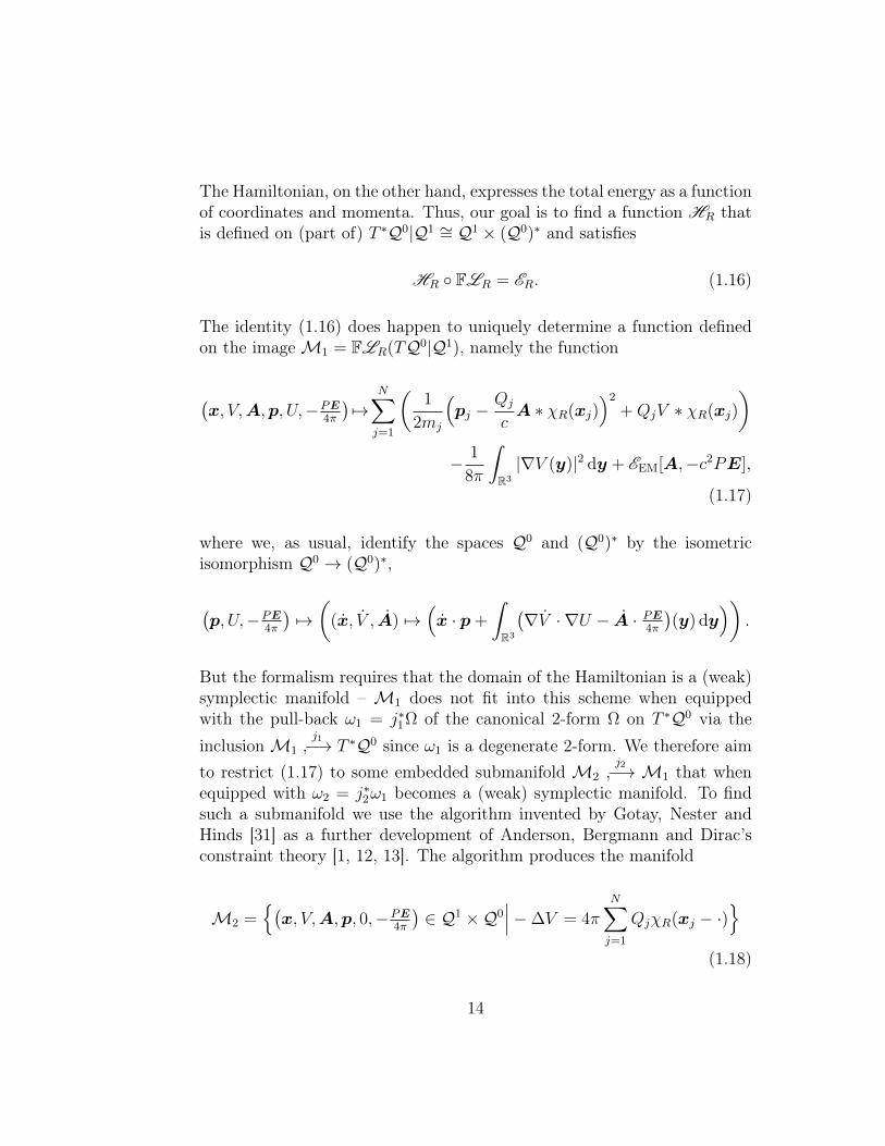
The Hamiltonian, on the other hand, expresses the total energy as a functionof coordinates and momenta. Thus, our goal is to find a function HR thatis defined on (part of) T ∗Q0|Q1 ∼= Q1 × (Q0)∗ and satisfies

HR FLR = ER. (1.16)

The identity (1.16) does happen to uniquely determine a function definedon the imageM1 = FLR(TQ0|Q1), namely the function

(x, V,A,p, U,−PE

4π

)7→

N∑

j=1

(1

2mj

(pj −

Qj

cA ∗ χR(xj)

)2+QjV ∗ χR(xj)

)

− 1

8π

∫

R3

|∇V (y)|2 dy + EEM[A,−c2PE],

(1.17)

where we, as usual, identify the spaces Q0 and (Q0)∗ by the isometricisomorphism Q0 → (Q0)∗,

(p, U,−PE

4π

)7→(

(x, V , A) 7→(x · p+

∫

R3

(∇V · ∇U − A · PE

4π

)(y) dy

)).

But the formalism requires that the domain of the Hamiltonian is a (weak)symplectic manifold – M1 does not fit into this scheme when equippedwith the pull-back ω1 = j∗1Ω of the canonical 2-form Ω on T ∗Q0 via theinclusionM1

j1−→ T ∗Q0 since ω1 is a degenerate 2-form. We therefore aim

to restrict (1.17) to some embedded submanifold M2

j2−→ M1 that when

equipped with ω2 = j∗2ω1 becomes a (weak) symplectic manifold. To findsuch a submanifold we use the algorithm invented by Gotay, Nester andHinds [31] as a further development of Anderson, Bergmann and Dirac’sconstraint theory [1, 12, 13]. The algorithm produces the manifold

M2 =(x, V,A,p, 0,−PE

4π

)∈ Q1 ×Q0

∣∣∣−∆V = 4πN∑

j=1

QjχR(xj − ·)

(1.18)

14

and restricting (1.17) to this manifold results in the function sending anelement

(x, V,A,p, 0,−PE

4π

)∈M2 into the number

N∑

j=1

1

2mj

(pj −

Qj

cA ∗ χR(xj)

)2+ EEM[A,−c2PE]

+N∑

j=1

N∑

k=1

QjQk

2

∫

R3

∫

R3

χR(xj − y)χR(xk − z)

|y − z| dy dz, (1.19)

where we have explicitly used that V is not an independent variable but isgiven uniquely in terms of x as the function z 7→∑N

j=1Qj

∫R3

χR(xj−y)|y−z| dy.

Due to this dependence of V on x we might as well identifyM2 with thespace R3N × PH1 × R3N × PL2 by the isomorphism

M2 3(x, V,A,p, 0,−PE

4π

)7→(x,A,p,−PE

4π

)∈ R3N × PH1 × R3N × PL2

and correspondingly let the Hamiltonian HR : R3N×PH1×R3N×PL2 → Rbe the function sending a given

(x,A,p,−PE

4π

)into the expression written

in (1.19).Having defined HR we will now take the point particle limit R → 0+.

The (j, k)’th term of the double sum in (1.19) represents the potentialenergy of particle j due to the Coulomb force exerted by particle k. Butin reality a given particle does not Coulomb interact with itself so it isreasonable to neglect the diagonal terms Q2

j

2R

∫R3

∫R3

χ(y)χ(z)|y−z| dy dz from the

Hamiltonian. The resulting function converges pointwise to

H0

(x,A,p,−PE

4π

)=

N∑

j=1

1

2mj

(pj −

Qj

cA(xj)

)2+

∑

1≤j<k≤N

QjQk

|xj − xk|+EEM[A,−c2PE],

(1.20)

at least ifA is continuous at x1, . . . ,xN . We are now in position to quantizethe charged particles in the model, which formally takes place by reinter-preting (1.20) as an (electromagnetic potential-dependent) operator on thequantum mechanical state space: For given

(A,−PE

4π

)∈ PH1×PL2 we thus

let the quantum mechanical Hamiltonian H(A,−PE

4π

)act as prescribed in

(1.20), where we perceive x = (x1, . . . ,xN) as the independent variableof functions belonging to the state space, we interpret A(xj), 1

|xj−xk| and

15

EEM[A,−c2PE] as multiplication operators acting on this space and we re-place pj by the differentiation operator −i~∇xj . The resulting Hamiltonianis exactly the one described in (1.7), where we under the Coulomb gaugecondition divA = 0 interpret the square

(i~∇xj +

QjcA(xj)

)2 as

(i~∇xj +

Qj

cA(xj)

)2= −~2∆xj + 2i

~Qj

cA(xj) · ∇xj +

Q2j

c2[A(xj)

]2

for j ∈ 1, . . . , N.Finally, to derive (1.8) we let ψ : R3N → C be a normalized state

and consider the average energy(A,−PE

4π

)7→(ψ,H

(A,−PE

4π

)ψ)L2 as a

classical Hamiltonian defined on the weak symplectic manifold PH1×PL2

equipped with the 2-form ω given by

ωm(m,A1,−PE1

4π,m,A2,−PE2

4π

)=

1

4π

∫

R3

(PE1 ·A2 − PE2 ·A1

)(y) dy

for m,(A1,−PE1

4π

),(A2,−PE2

4π

)∈ PH1 × PL2. The associated Hamilton

equations read

1

c2∂tA(t) = −PE(t) and − ∂tPE(t) = ∆A(t) +

4π

c

N∑

j=1

PJSj [ψ,A(t)].

(1.21)

Here, the electromagnetic field is regarded as a dynamic quantity, while thewave function ψ is considered to be fixed in time. However, according tothe postulates of quantum mechanics the state ψ is also expected to evolvein time, namely as governed by the Schrödinger equation

i~∂tψ(t) = H(A(t),−PE(t)

4π

)ψ(t). (1.22)

The system (1.8) can now be obtained by coupling (1.21) with (1.22) inthe sense that we replace the fixed ψ appearing in (1.21) with the time-dependent ψ(t) that is present in (1.22).

The many-body Maxwell-Pauli SystemIf all of the N particles have spin 1

2and we describe their kinetic energies by

means of the Pauli operator then the (electromagnetic potential-dependent)

16

Hamiltonian of the system is given by

H(A,−PE

4π

)=

N∑

j=1

(σ ·(i~∇xj +

QjcA(xj)

))2

2mj

+∑

1≤j<k≤N

QjQk

|xj − xk|+EEM[A,−c2PE]

and the corresponding many-body Maxwell-Pauli system expressed in Cou-lomb gauge reads

A =4π

c

N∑

j=1

PJPj [ψ,A],

i~∂tψ =

(N∑

j=1

(σ ·(i~∇xj +

QjcA(xj)

))2

2mj

+∑

1≤j<k≤N

QjQk

|xj − xk|

)ψ

+ EEM[A, ∂tA]ψ,

divA = 0.

(1.23)

Here, the `’th component of the current density JPj [ψ,A](t) : R3 → R3 is

for ` ∈ 1, 2, 3 given byJPj [ψ,A](t)

`(xj)

= −Qj

mj

∑

s∈1,2N

3∑

k=1

2∑

v=1

2∑

w=1

Re

∫

R3(N−1)

ψ(t)

(s1,...,sj ,...,sN )(x1, . . . ,xj, . . . ,xN)

· σ`sjwσkwv(i~∂xkj +

Qj

cAk(t)(xj)

)ψ(t)

(s1,...,v,...,sN )(x1, . . . ,xj, . . . ,xN) dx′j,

where xj = (x1j , x2j , x

3j), x′j = (x1, . . . ,xj−1,xj+1, . . . ,xN), σk =

(σkwv)2w,v=1

,A = (A1, A2, A3) and s = (s1, . . . , sN) for (j, k) ∈ 1, . . . , N × 1, 2, 3.

For simplicity let us consider the one-body Maxwell-Pauli system thatmodels a single spin-1

2particle of mass m > 0 and charge Q ∈ R \ 0

interacting with it’s self-generated electromagnetic field. By using the Lich-nerowicz formula (1.2) we can formulate this system in Coulomb gauge as

A =4π

cPJP[ψ,A],

i~∂tψ =

(1

2m

(i~∇+

Q

cA)2− ~Q

2mcσ · ∇ ×A+ EEM[A, ∂tA]

)ψ,

divA = 0

(1.24)

17

and the probability current density JP[ψ,A](t) : R3 → R3 reduces to

JP[ψ,A](t)(x) = −Qm

Re⟨ψ(t)(x),

(i~∇+

Q

cA)ψ(t)(x)

⟩C2

+~Q2m∇×

⟨ψ(t)(x),σψ(t)(x)

⟩C2 .

Note that this system only differs from the (N = 1)-case of (1.8) by thepresence of − ~Q

2mcσ ·∇×Aψ in (1.24) and the presence of ~Q

2m∇×

⟨ψ,σψ

⟩C2

in the expression for the probability current density. To our knowledge thewell-posedness of the Maxwell-Pauli system has not yet been studied byanyone, even in the simplest case N = 1. We have tried several differentapproaches to proving local in time existence of a solution to the Cauchyproblem associated with (1.24), but all of these methods seem to breakdown due to the presence of the two derivative-terms mentioned above.Instead, we have turned to the problem of proving existence of travellingwave solutions to the one-body Maxwell-Pauli (and Maxwell-Schrödinger)system, as explained in the following section.

Travelling WavesUntil now we have only considered whether the laws of quantum mechanicsand electrodynamics admit matter to exist and evolve in time. But inorder to give an appropriate description of reality these laws also oughtto predict particle motions that correspond with our expectations. Forinstance, we expect a single charged particle to be able to move in spaceat a constant velocity v ∈ R3, while still obeying the Maxwell equationsas well as the Schrödinger equation. Put another way, there should exist asolution (ψt,At) to the (N = 1)-case of (1.8) (or (1.24)) in the form

ψt(t)(x) = e−iωtψ(x− vt),At(t)(x) = A(x− vt), (1.25)

where (ψ,A) is defined on R3 and ω is a real number. Such a solution(ψt,At) is called a travelling wave solution for obvious reasons.

Objective 2 : Given any appropriate velocity v ∈ R3 prove that wecan find an ω ∈ R such that the pair (ψt,At) defined in (1.25) solvesthe (N = 1)-case of (1.8) (or (1.24)).

18

Under suitable conditions on the velocity v we manage to meet Objective2 in [56]. If the particle were uncharged it’s total energy would naturallybe given by 1

2m|v|2 as a function of the speed |v| of motion. But a particle

with nonzero charge has to drag it’s self-generated electromagnetic fieldalong with it – to what extent does this affect the dependence of the totalenergy on the speed |v|? We provide an answer to this question in [56].

19

Overview of the Results 2We will now state the precise results of the two papers contained in thisthesis. For a more indepth explanation of the notation we refer the readerto the Introduction.

Existence of a Unique Local Solution to theMany-body Maxwell-Schrödinger InitialValue ProblemThe many-body Maxwell-Schrödinger system, describing a system of Ncharged particles, reads

A =4π

c

N∑

j=1

PJj[ψ,A],

i~∂tψ =

(N∑

j=1

(i~∇xj +

QjcA(xj)

)2

2mj

+∑

1≤j<k≤N

QjQk

|xj − xk|+ EEM[A, ∂tA]

)ψ,

(2.1)

where A(t) : R3 → R3 is the magnetic vector potential expected to satisfythe Coulomb gauge condition divA(t) = 0 at all times, ψ(t) : R3N → C isthe quantum mechanical wave function and Jj[ψ,A](t) : R3 → R3 is theprobability current density

xj 7→(−Qj

mj

Re

∫

R3(N−1)

ψ(t)(x)(i~∇xj +

Qj

cA(t)(xj)

)ψ(t)(x) dx′j

)

20

associated with the j’th particle. It seems that well-posedness questionsconcerning this system have not yet been considered in the literature. Onthe other hand, several authors have studied the d-dimensional Maxwell-Schrödinger system

−∆dϕ−1

c∂tdivdA = 4πQ|ψ|2,

dA+∇d

(1

c∂tϕ+ divdA

)= −4π

c

Q

mRe(ψ(i~∇d +

Q

cA)ψ),

i~∂tψ =( 1

2m

(i~∇d +

Q

cA)2

+Qϕ)ψ,

(2.2)

where (ψ, ϕ,A)(t) : Rd → C × R × Rd, ∆d =∑d

k=1 ∂2xk, d = 1

c2∂2t − ∆d,

∇d = (∂x1 , . . . , ∂xd) and divdA =∑d

k=1 ∂xkAk. However, the known results

concerning (2.2) can not be directly applied to (2.1) due to the presence ofthe Coulomb singularities 1

|xj−xk| in (2.1). For d = 3 the system (2.2) canbe expressed in Coulomb gauge by

A =4π

cP(−Qm

Re(ψ(i~∇+

Q

cA)ψ))

i~∂tψ =( 1

2m

(i~∇+

Q

cA)2

+Q2(|x|−1 ∗ |ψ|2

))ψ,

(2.3)

which only deviates from the (N = 1)-case of (2.1) by the presence of theterm Q2

(|x|−1 ∗ |ψ|2

)ψ and the absence of the term EEM[A, ∂tA] on the

right hand side of (2.3)’s second equation. The term Q2(|x|−1 ∗ |ψ|2

)ψ

should definitely not be included in the equations of motion describing asingle charged particle so at least in this simple case (2.1) is evidently abetter description of reality than (2.3). Nakamitsu and Tsutsumi treat(2.2) expressed in Lorenz gauge in the paper [52], where they prove localwell-posedness of the system for all dimensions d and in the special casesd ∈ 1, 2 they even prove global well-posedness. The well-posedness theoryregarding (2.2) is developed further in the papers [27, 28, 29, 30, 33, 52, 53,54, 57, 61] and the research culminates with Bejenaru and Tataru [2] provingglobal well-posedness in the energy space of the three-dimensional version of(2.2) expressed in Coulomb gauge and with Wada [62] proving the analogousresult for the two-dimensional variant of (2.2) expressed in Lorenz gauge.Our main result concerning the many-body Maxwell-Schrödinger systemsays the following.

21

Theorem 1. Let (ψ0,A0,A1) ∈ H2(R3N)×H 32 (R3;R3)×H 1

2 (R3;R3) sat-isfy divA0 = divA1 = 0. Then there exist a T > 0 and a unique (ψ,A) inC([0, T ];H2(R3N)) ×

(C([0, T ];H

32 (R3;R3)) ∩ C1([0, T ];H

12 (R3;R3))

)that

solves (2.1), fulfills the condition divA(t) = 0 for all t ∈ [0, T ], and takesthe values

ψ(0) = ψ0,A(0) = A0 and ∂tA(0) = A1

at time t = 0.

To prove Theorem 1 we use the same strategy as in [53, 54]: We first intro-duce a solution mapping (ψ,A) 7→ (ξ,B) associated with the linearization

( + 1)B =4π

c

N∑

j=1

PJj[ψ,A] +A (2.4)

i~∂tξ =( N∑

j=1

1

2mj

(i~∇xj +

Qj

cA(xj)

)2+

∑

1≤j<k≤N

QjQk

|xj − xk|)ξ,

(2.5)

of (2.1) supplied with the initial conditions

ξ(0) = ψ0, B(0) = A0 and ∂tB(0) = A1.

Then we show that this mapping is a contraction on an appropriate completenormed space – this implies the desired result by the Banach fixed-pointtheorem. The solution operator corresponding to (2.5) is defined by meansof Kato’s result [34, 35] concerning Cauchy problems related to quite generallinear evolution equations – the required estimate on a certain norm of thisoperator is obtained by using Gronwall’s inequality. To treat the solution tothe linear Klein-Gordon equation (2.4) we use a known Strichartz estimate[4, 25, 26, 60].

Existence of Travelling Wave Solutions tothe Maxwell-Pauli and Maxwell-SchrödingerSystemsIn this paper that is joint work with Jan Philip Solovej, we prove the exist-ence of travelling wave solutions to the Maxwell-Schrödinger system (j = S)

22

provided that the velocity of the wave is not too large – we also prove theanalogous result for the Maxwell-Pauli system (j = P). These systems canbe formulated in Coulomb gauge as

At =4π

cPJj[ψt,At],

i~∂tψt =( 1

2m∇2j,At

+ EEM[At, ∂tAt])ψt

(2.6)

for j ∈ S,P, where ψt(t) : R3 → C2 denotes the spinor wave function, themagnetic vector potential At(t) : R3 → R3 should satisfy divAt(t) = 0 atall times t and we use the abbreviations

∇j,At =

i~∇+Q

cAt for j = S

σ ·(i~∇+

Q

cAt

)for j = P

as well as

Jj[ψt,At](t)(x) =

−Qm

Re⟨ψt(t)(x),∇S,Atψt(t)(x)

⟩C2 for j = S

−Qm

Re⟨ψt(t)(x),σ∇P,Atψt(t)(x)

⟩C2 for j = P

.

By a travelling wave – at velocity v ∈ R3 – we mean a pair (ψt,At) thatcan be written in the form

ψt(t)(x) = e−iωtψ(x− vt),At(t)(x) = A(x− vt)

for some real number ω and some time independent (ψ,A) : R3 → C2×R3.There are not that many known results concerning travelling wave solu-tions to the equations of motion for a single charged particle. Coclite andGeorgiev prove in [8] that the three-dimensional version of (2.2) expressedin Lorenz gauge has no nontrivial solutions (ψt,At, ϕt) in the form

ψt(t)(x) = e−iωtψ(x),

At(t)(x) = 0,

ϕt(t)(x) = ϕ(x)

23

and they also find that such solutions do exist when one adds to theSchrödinger equation a potential energy term originating from an attractiveCoulomb force. In the paper [3], Benci and Fortunato study the correspond-ing problem in a bounded space region and in [16], Esteban, Georgiev andSéré prove the existence of stationary solutions to the Maxwell-Dirac andKlein-Gordon-Dirac systems. Finally, we mention that Fröhlich, Jonssonand Lenzmann [23] show the existence of travelling solitary wave solutionsto an equation describing the dynamics of pseudo-relativistic boson stars inthe mean field limit – again under a smallness assumption on the speed ofthe wave. As mentioned above the system (2.6) serves as a better descrip-tion of a single charged particle than (2.2) – the existence of travelling wavesolutions to (2.6) has never been studied before. Let us formulate our maintheorem concerning the Maxwell-Schrödinger system. We remind the readerthat H1(R3;C2) denotes the usual Sobolev space of order 1 and D1(R3;R3)denotes the space of locally integrable maps R3 → R3 that vanish at infinityand have square integrable first derivatives.

Theorem 2. For all λ > 0 and v ∈ R3 with 0 < |v| < c there existω ∈ R and (ψ,A) ∈ H1(R3;C2) × D1(R3;R3) satisfying ‖ψ‖2L2 = λ anddivA = 0 such that (ψt,At)(t)(x) =

(e−iωtψ(x−vt),A(x−vt)

)solves the

(j = S)-case of (2.6).

Here, λ = 1 is the physically relevant case since ‖ψ‖2L2 should be interpretedas the total probability that the charged particle is located somewhere in R3.We see that the Maxwell-Schrödinger system admits charged particles (andtheir self-generated electromagnetic fields) to travel with nonzero speedsless than that of the light’s – this upper bound on the allowed speeds ofmotion is in agreement with the special theory of relativity so travellingwave solutions to (2.6) with |v| ≥ c do most likely not exist. However, wehave not proven this. Our main theorem about the Maxwell-Pauli systemsays the following – we let KS be the constant occurring in the Sobolevinequality ‖A‖L6 ≤ KS‖∇A‖L2 .

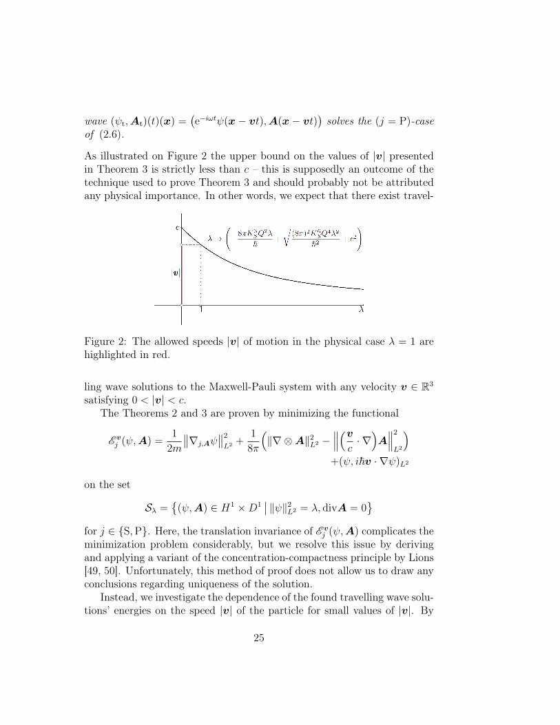
Theorem 3. Consider an arbitrary λ > 0 as well as some given velocityv ∈ R3 satisfying

0 < |v| < −8πK3SQ

2λ

~+

√(8π)2K6

SQ4λ2

~2+ c2.

Then there exist an ω ∈ R and a pair (ψ,A) ∈ H1(R3;C2) × D1(R3;R3)fulfilling the identities ‖ψ‖2L2 = λ and divA = 0 such that the travelling

24

wave (ψt,At)(t)(x) =(e−iωtψ(x− vt),A(x− vt)

)solves the (j = P)-case

of (2.6).

As illustrated on Figure 2 the upper bound on the values of |v| presentedin Theorem 3 is strictly less than c – this is supposedly an outcome of thetechnique used to prove Theorem 3 and should probably not be attributedany physical importance. In other words, we expect that there exist travel-

Figure 2: The allowed speeds |v| of motion in the physical case λ = 1 arehighlighted in red.

ling wave solutions to the Maxwell-Pauli system with any velocity v ∈ R3

satisfying 0 < |v| < c.The Theorems 2 and 3 are proven by minimizing the functional

E vj (ψ,A) =

1

2m

∥∥∇j,Aψ∥∥2L2 +

1

8π

(‖∇ ⊗A‖2L2 −

∥∥∥(vc· ∇)A∥∥∥2

L2

)

+(ψ, i~v · ∇ψ)L2

on the set

Sλ =

(ψ,A) ∈ H1 ×D1∣∣ ‖ψ‖2L2 = λ, divA = 0

for j ∈ S,P. Here, the translation invariance of E vj (ψ,A) complicates the

minimization problem considerably, but we resolve this issue by derivingand applying a variant of the concentration-compactness principle by Lions[49, 50]. Unfortunately, this method of proof does not allow us to draw anyconclusions regarding uniqueness of the solution.

Instead, we investigate the dependence of the found travelling wave solu-tions’ energies on the speed |v| of the particle for small values of |v|. By

25

the energy of a (sufficiently nice) solution (ψt,At) to (2.6) we here meanthe average

(ψt,Hj

(At,

∂tAt

4πc2

)ψt

)L2 of the energy observable given by

Hj

(A,−PE

4π

)=

1

2m∇2j,A + EEM[A,−c2PE].

For travelling wave solutions (ψt,At)(t)(x) =(e−iωtψ(x− vt),A(x− vt)

)

the energy takes the form

Ej(v, ψ,A) =1

2m‖∇j,Aψ‖2L2 +

1

8π

∫

R3

(|∇ ×A|2 +

∣∣∣(vc· ∇)A∣∣∣2)

dxλ.

We have found the following result concerning this energy function.

Theorem 4. Let j ∈ S,P and λ > 0 be arbitrary. Then there existuniversal constants θj, κj > 0 such that the inequality

∣∣∣Ej(v, ψ,A)− mv2

2λ∣∣∣ ≤ κj|v|3

holds for all velocities v ∈ R3 with 0 < |v| < θj and all minimizers (ψ,A)of E v

j on Sλ.

Thus, the energy of the charged particle essentially behaves as if the particlewere uncharged (for small velocities).

26

Conclusions andPerspectives 3

Let us now mention some interesting problems that are related to the onesstudied in this thesis and would be natural to pursue in further research.

Problem 1: Global well-posedness of themany-body Maxwell-Schrödinger System

In [55], we have shown local existence of a unique solution to the many-bodyMaxwell-Schrödinger initial value problem expressed in Coulomb gauge. Asis apparent from Theorem 1 the triple (ψ0,A0,A1) of initial data is requiredto belong to H2(R3N)×H 3

2 (R3;R3)×H 12 (R3;R3) and then as a function of

time the corresponding solution (ψ,A, ∂tA) will map continuously into thesame space. However, it would be desirable to derive the same result for aspace of less regularity, for instance H2(R3N)×H1(R3;R3)×L2(R3;R3) orH2(R3N) × D1(R3;R3) × L2(R3;R3). On another note, our intuition tellsus that changing the initial data a “little bit” should only imply a “small”change in the solution. It would be desirable to confirm this intuition byshowing that the solution depends continuously on the initial data. Finally,we would like to prove that the solution exists globally in time.

27

Problem 2: Well-posedness of theMaxwell-Pauli systemAs already mentioned, even proving the existence of a local solution to theone-body Maxwell-Pauli initial value problem is an open problem. Well-posedness of the Maxwell-Pauli system is an intriguing topic, especiallywhen seen in the light of the already known results concerning energeticstability. Remember that systems of charged particles with Pauli kineticenergy are only energetically stable under certain conditions on the fine-structure constant and on the atomic numbers of the nuclei. This raisessome interesting questions regarding the influence of these parameters onthe well-posedness of the Maxwell-Pauli system. Does global (or even local)well-posedness for instance fail to hold for large values of α? We do notknow.

Problem 3: Uniqueness of travelling wavesolutionsIn [56], we prove the existence of travelling wave solutions to the Maxwell-Schrödinger and Maxwell-Pauli systems, provided that the speed of thewave is not too large – this is done by minimizing some functional E v

j ona certain set. The solution produced by this method is clearly not uniquedue to translation invariance of E v

j , but it would be satisfactory to showuniqueness of the solution up to symmetries.

28

Bibliography

[1] James L. Anderson and Peter G. Bergmann. Constraints in covariantfield theories. Physical Rev. (2), 83:1018–1025, 1951.

[2] Ioan Bejenaru and Daniel Tataru. Global wellposedness in the en-ergy space for the Maxwell-Schrödinger system. Comm. Math. Phys.,288(1):145–198, 2009.

[3] Vieri Benci and Donato Fortunato. An eigenvalue problem for theSchrödinger-Maxwell equations. Topol. Methods Nonlinear Anal.,11(2):283–293, 1998.

[4] Philip Brenner. On space-time means and everywhere defined scat-tering operators for nonlinear Klein-Gordon equations. Math. Z.,186(3):383–391, 1984.

[5] David Brydges and Paul Federbush. A note on energy bounds for bosonmatter. J. Mathematical Phys., 17(12):2133–2134, 1976.

[6] Luca Bugliaro, Charles Fefferman, and Gian Michele Graf. A Lieb-Thirring bound for a magnetic Pauli Hamiltonian. II. Rev. Mat.Iberoamericana, 15(3):593–619, 1999.

[7] Luca Bugliaro, Jürg Fröhlich, and Gian Michele Graf. Stability ofquantum electrodynamics with nonrelativistic matter. Phys. Rev. Lett.,77:3494–3497, Oct 1996.

[8] Giuseppe Maria Coclite and Vladimir Georgiev. Solitary waves forMaxwell-Schrödinger equations. Electron. J. Differential Equations,pages No. 94, 31 pp. (electronic), 2004.

29

[9] Joseph G. Conlon. The ground state energy of a classical gas. Comm.Math. Phys., 94(4):439–458, 1984.

[10] Joseph G. Conlon, Elliott H. Lieb, and Horng-Tzer Yau. The N7/5 lawfor charged bosons. Comm. Math. Phys., 116(3):417–448, 1988.

[11] Ingrid Daubechies and Elliott H. Lieb. One-electron relativistic mo-lecules with Coulomb interaction. Comm. Math. Phys., 90(4):497–510,1983.

[12] P. A. M. Dirac. Generalized Hamiltonian dynamics. Canadian J.Math., 2:129–148, 1950.

[13] P. A. M. Dirac. Generalized Hamiltonian dynamics. Proc. Roy. Soc.London. Ser. A, 246:326–332, 1958.

[14] Freeman J. Dyson. Ground-state energy of a finite system of chargedparticles. J. Math. Phys., 8(8):1538–1545, 1967.

[15] Freeman J. Dyson and A. Lenard. Stability of matter. I. J. Math.Phys., 8(3):423–434, 1967.

[16] Maria J. Esteban, Vladimir Georgiev, and Eric Séré. Stationary solu-tions of the Maxwell-Dirac and the Klein-Gordon-Dirac equations.Calc. Var. Partial Differential Equations, 4(3):265–281, 1996.

[17] Paul Federbush. A new approach to the stability of matter problem. I,II. J. Mathematical Phys., 16:347–351; ibid. 16 (1975), 706–709, 1975.

[18] C. Fefferman and R. de la Llave. Relativistic stability of matter. I.Rev. Mat. Iberoamericana, 2(1-2):119–213, 1986.

[19] Charles Fefferman. Stability of Coulomb systems in a magnetic field.Proc. Nat. Acad. Sci. U.S.A., 92(11):5006–5007, 1995.

[20] Charles Fefferman. On electrons and nuclei in a magnetic field. Adv.Math., 124(1):100–153, 1996.

[21] Charles Fefferman, Jürg Fröhlich, and Gian Michele Graf. Stability ofultraviolet-cutoff quantum electrodynamics with non-relativistic mat-ter. Comm. Math. Phys., 190(2):309–330, 1997.

30

[22] Rupert L. Frank, Elliott H. Lieb, and Robert Seiringer. Stability ofrelativistic matter with magnetic fields for nuclear charges up to thecritical value. Comm. Math. Phys., 275(2):479–489, 2007.

[23] Jürg Fröhlich, B. Lars G. Jonsson, and Enno Lenzmann. Boson starsas solitary waves. Comm. Math. Phys., 274(1):1–30, 2007.

[24] Jürg Fröhlich, Elliott H. Lieb, and Michael Loss. Stability of Coulombsystems with magnetic fields. I. The one-electron atom. Comm. Math.Phys., 104(2):251–270, 1986.

[25] J. Ginibre and G. Velo. Time decay of finite energy solutions of the non-linear Klein-Gordon and Schrödinger equations. Ann. Inst. H. PoincaréPhys. Théor., 43(4):399–442, 1985.

[26] J. Ginibre and G. Velo. Generalized Strichartz inequalities for the waveequation. In Partial differential operators and mathematical physics(Holzhau, 1994), volume 78 of Oper. Theory Adv. Appl., pages 153–160. Birkhäuser, Basel, 1995.

[27] J. Ginibre and G. Velo. Long range scattering and modified waveoperators for the Maxwell-Schrödinger system. I. The case of vanishingasymptotic magnetic field. Comm. Math. Phys., 236(3):395–448, 2003.

[28] J. Ginibre and G. Velo. Long range scattering for the Maxwell-Schrödinger system with arbitrarily large asymptotic data. HokkaidoMath. J., 37(4):795–811, 2008.

[29] Jean Ginibre and Giorgio Velo. Long range scattering for theMaxwell-Schrödinger system with large magnetic field data and smallSchrödinger data. Publ. Res. Inst. Math. Sci., 42(2):421–459, 2006.

[30] Jean Ginibre and Giorgio Velo. Long range scattering and modifiedwave operators for the Maxwell-Schrödinger system. II. The generalcase. Ann. Henri Poincaré, 8(5):917–994, 2007.

[31] Mark J. Gotay, James M. Nester, and George Hinds. Presymplecticmanifolds and the Dirac-Bergmann theory of constraints. J. Math.Phys., 19(11):2388–2399, 1978.

31

[32] Marcel Griesemer and Christian Tix. Instability of a pseudo-relativisticmodel of matter with self-generated magnetic field. J. Math. Phys.,40(4):1780–1791, 1999.

[33] Yan Guo, Kuniaki Nakamitsu, and Walter Strauss. Global finite-energysolutions of the Maxwell-Schrödinger system. Comm. Math. Phys.,170(1):181–196, 1995.

[34] Tosio Kato. Linear evolution equations of “hyperbolic” type. J. Fac.Sci. Univ. Tokyo Sect. I, 17:241–258, 1970.

[35] Tosio Kato. Linear evolution equations of “hyperbolic” type. II. J.Math. Soc. Japan, 25:648–666, 1973.

[36] J. L. Lebowitz and Elliott H. Lieb. Existence of thermodynamics forreal matter with coulomb forces. Phys. Rev. Lett., 22:631–634, Mar1969.

[37] A. Lenard and Freeman J. Dyson. Stability of matter. II. J. Math.Phys., 9(5):698–711, 1968.

[38] Elliott H. Lieb. The N5/3 law for bosons. Phys. Lett. A, 70(2):71–73,1979.

[39] Elliott H. Lieb and Joel L. Lebowitz. The constitution of matter:Existence of thermodynamics for systems composed of electrons andnuclei. Advances in Math., 9:316–398, 1972.

[40] Elliott H. Lieb and Michael Loss. Stability of Coulomb systems withmagnetic fields. II. The many-electron atom and the one-electron mo-lecule. Comm. Math. Phys., 104(2):271–282, 1986.

[41] Elliott H. Lieb and Michael Loss. Stability of a model of relativisticquantum electrodynamics. Comm. Math. Phys., 228(3):561–588, 2002.

[42] Elliott H. Lieb, Michael Loss, and Heinz Siedentop. Stability of relativ-istic matter via Thomas-Fermi theory. Helv. Phys. Acta, 69(5-6):974–984, 1996. Papers honouring the 60th birthday of Klaus Hepp and ofWalter Hunziker, Part I (Zürich, 1995).

[43] Elliott H. Lieb, Michael Loss, and Jan Philip Solovej. Stability ofmatter in magnetic fields. Phys. Rev. Lett., 75(6):985–989, 1995.

32

[44] Elliott H. Lieb and Robert Seiringer. The stability of matter in quantummechanics. Cambridge University Press, Cambridge, 2010.

[45] Elliott H. Lieb, Heinz Siedentop, and Jan Philip Solovej. Stability andinstability of relativistic electrons in classical electromagnetic fields. J.Statist. Phys., 89(1-2):37–59, 1997. Dedicated to Bernard Jancovici.

[46] Elliott H. Lieb and Jan Philip Solovej. Ground state energy of the two-component charged Bose gas. Comm. Math. Phys., 252(1-3):485–534,2004.

[47] Elliott H. Lieb and Walter E. Thirring. Bound for the kinetic energyof fermions which proves the stability of matter. Phys. Rev. Lett.,35:687–689, Sep 1975.

[48] Elliott H. Lieb and Horng-Tzer Yau. The stability and instability ofrelativistic matter. Comm. Math. Phys., 118(2):177–213, 1988.

[49] P.-L. Lions. The concentration-compactness principle in the calculus ofvariations. The locally compact case. I. Ann. Inst. H. Poincaré Anal.Non Linéaire, 1(2):109–145, 1984.

[50] P.-L. Lions. The concentration-compactness principle in the calculus ofvariations. The locally compact case. II. Ann. Inst. H. Poincaré Anal.Non Linéaire, 1(4):223–283, 1984.

[51] Michael Loss and Horng-Tzer Yau. Stabilty of Coulomb systems withmagnetic fields. III. Zero energy bound states of the Pauli operator.Comm. Math. Phys., 104(2):283–290, 1986.

[52] Kuniaki Nakamitsu and Masayoshi Tsutsumi. The Cauchy prob-lem for the coupled Maxwell-Schrödinger equations. J. Math. Phys.,27(1):211–216, 1986.

[53] Makoto Nakamura and Takeshi Wada. Local well-posedness for theMaxwell-Schrödinger equation. Math. Ann., 332(3):565–604, 2005.

[54] Makoto Nakamura and Takeshi Wada. Global existence and unique-ness of solutions to the Maxwell-Schrödinger equations. Comm. Math.Phys., 276(2):315–339, 2007.

33

[55] Kim Petersen. Existence of a Unique Local Solution to the Many-bodyMaxwell-Schrödinger Initial Value Problem. Preprint 2013.

[56] Kim Petersen and Jan Philip Solovej. Existence of Travelling WaveSolutions to the Maxwell-Pauli and Maxwell-Schrödinger Systems.Preprint 2013.

[57] Akihiro Shimomura. Modified wave operators for Maxwell-Schrödingerequations in three space dimensions. Ann. Henri Poincaré, 4(4):661–683, 2003.

[58] Jan Philip Solovej. Upper bounds to the ground state energies of theone- and two-component charged Bose gases. Comm. Math. Phys.,266(3):797–818, 2006.

[59] Herbert Spohn. Dynamics of charged particles and their radiation field.Cambridge University Press, Cambridge, 2004.

[60] Robert S. Strichartz. Restrictions of Fourier transforms to quadraticsurfaces and decay of solutions of wave equations. Duke Math. J.,44(3):705–714, 1977.

[61] Yoshio Tsutsumi. Global existence and asymptotic behavior of solu-tions for the Maxwell-Schrödinger equations in three space dimensions.Comm. Math. Phys., 151(3):543–576, 1993.

[62] Takeshi Wada. Smoothing effects for Schrödinger equationswith electro-magnetic potentials and applications to the Maxwell-Schrödinger equations. J. Funct. Anal., 263(1):1–24, 2012.

34

Existence of a Unique Local Solutionto the Many-body

Maxwell-Schrödinger Initial ValueProblem

Kim Petersen

Department of Mathematical Sciences, University of Copenhagen,Universitetsparken 5, DK-2100 Copenhagen, Denmark, Email: kp@math.ku.dk

c© 2013 by the author

Abstract. We study the many-body problem of charged particlesinteracting with their self-generated electromagnetic field. We modelthe dynamics of the particles by the many-body Maxwell-Schrödingersystem, where the particles are treated quantum mechanically and theelectromagnetic field is a classical quantity. We prove the existence of aunique local in time solution to this nonlinear initial value problem usinga contraction mapping argument.

Mathematics Subject Classification 2010: 81V70, 35Q41, 35Q61

1 Introduction

The three-dimensional many-body Maxwell-Schrödinger system in Coulombgauge is a system of partial differential equations that models the dynamics ofseveral charged point particles interacting via their self-generated electromag-netic fields – in Gaussian units it reads

A =4π

c

N∑

j=1

PJj [ψ,A],

i~∂tψ =( N∑

j=1

1

2mj∇2j,A +

∑

1≤j<k≤N

QjQk|xj − xk|

+ EEM[A, ∂tA])ψ,

(1)

where ~ > 0 is the reduced Planck constant, c > 0 is the speed of light, N ∈ N isthe number of particles, m1, . . . ,mN > 0 are the particles’ respective masses,Q1, . . . , QN ∈ R are their charges, ψ(t) : R3N → C is the wave function,

35

A(t) : R3 → R3 is the vector potential, ∇j,A = i~∇xj +Qjc A(xj) is the

covariant derivative with respect toA acting on the j’th particle, = 1c2∂2t −∆

denotes the d’Alembertian, P = 1 − ∇div∆−1 is the Helmholtz projection,EEM[A, ∂tA](t) is the field energy

EEM[A, ∂tA](t) =1

8π

∫

R3

(|∇ ×A(t)(y)|2 +

∣∣∣1c∂tA(t)(y)

∣∣∣2)

dy

and Jj [ψ,A](t) denotes the j’th particle’s probability current density

Jj [ψ,A](t) : R3 3 xj 7→(−Qjmj

Re

∫

R3(N−1)

ψ(t)(x)∇j,Aψ(t)(x) dx′j)∈ R3

where x = (x1, . . . ,xN ) and x′j = (x1, . . . ,xj−1,xj+1, . . . ,xN ). That we havechosen Coulomb gauge means that the magnetic vector potential A shouldsatisfy

divA(t) = 0. (2)

As we will see later we might just as well study the system

A =4π

c

N∑

j=1

PJj [ψ,A],

i~∂tψ =( N∑

j=1

1

2mj∇2j,A +

∑

1≤j<k≤N

QjQk|xj − xk|

)ψ,

(3)

where the field energy-term EEM[A, ∂tA] is no longer present in the Schrödingerequation. In the literature the d-dimensional Maxwell-Schrödinger system of-ten refers to the coupled equations

−∆dϕ−1

c∂tdivdA = 4πQ|ψ|2,

dA+∇d(1

c∂tϕ+ divdA

)= −4π

c

Q

mRe(ψ(i~∇d +

Q

cA)ψ),

i~∂tψ =( 1

2m

(i~∇d +

Q

cA)2

+Qϕ)ψ,

(4)

with unknowns ψ(t) : Rd → C, A(t) : Rd → Rd, ϕ(t) : Rd → R and a hopefullyobvious notation. If d = 3 and A satisfies the Coulomb gauge-condition (2)the system (4) reads

A = P(−4π

c

Q

mRe(ψ(i~∇+

Q

cA)ψ)),

i~∂tψ =( 1

2m

(i~∇+

Q

cA)2

+Q2(|x|−1 ∗ |ψ|2

))ψ,

(5)

36

which only differs from the (N = 1)-case of (3) by the presence of the nonlinearterm Q2(|x|−1 ∗ |ψ|2)ψ in the Schrödinger equation. This term comes from theparticles’ Coulomb self-interactions. From a physical point of view it is wrongto include self-interactions in this context. In fact, the system (5) may beconsidered as a mean field approximation to the many-body description (3).In the (c→∞)-limit the second equation in (3) reduces to the standard many-body Coulomb problem

i~∂tψ =(−

N∑

j=1

~2

2mj∆xj +

∑

1≤j<k≤N

QjQk|xj − xk|

)ψ

which is the basis of almost all work done in quantum chemistry. On theother hand, the system (5) reduces in the (c → ∞)-limit to a mean fieldapproximation, which at best would be good in the large N limit. The system(4) has been studied (up to different choices of units) by several authors, bothwhen expressed in the Coulomb gauge [4, 12, 13, 14, 15, 17, 21, 22, 24, 28],the Lorenz gauge [17, 20, 21, 22, 29] and the temporal gauge [17, 21, 22]. In[20], Nakamitsu and Tsutsumi prove local well-posedness in sufficiently regularSobolev spaces of the d-dimensional Maxwell-Schrödinger initial value problem– for d ∈ 1, 2 they also show global existence of the solution. Tsutsumi showsin [28] that for d = 3 the problem has a global solution for a certain set offinal states (i.e. data given at t = +∞) and studies the asymptotic behavior ofsuch a solution. In [17], Guo, Nakamitsu and Strauss prove global solvabilityof the three-dimensional system in Coulomb gauge (but not uniqueness of thesolution) for initial data (ψ(0),A(0), ∂tA(0)) in the space of H1 × H1 × L2-functions satisfying divA(0) = div∂tA(0) = 0. Using techniques on which thearguments in the present paper are based, Nakamura and Wada [21] prove localwell-posedness of the three-dimensional problem in Sobolev spaces of sufficientregularity, expanding significantly on the previously known results – in [22]they even prove global existence of unique solutions. Bejenaru and Tataru [4]prove global well-posedness in the energy-space of the three-dimensional initialvalue problem and in the recent paper [29], Wada proves unique solvability inthe energy space of the two-dimensional analogue. The scattering theory for(5) has also been studied by several authors – see the papers by Tsutsumi [28],Shimomura [24] as well as Ginibre and Velo [12, 13, 14, 15]. It seems that thesolvability of the system (1) has not yet been studied and the known resultsconcerning (4) are not directly applicable to this system due to the presence ofthe Coulomb singularities 1

|xj−xk| in (1). The aim of this paper is to prove theunique existence of a local solution to (1) as expressed in the following maintheorem.

Theorem 1. For all (ψ0,A0,A1) ∈ H2(R3N ) × H32 (R3;R3) × H

12 (R3;R3)

with divA0 = divA1 = 0 there exist a number T > 0 and a unique solution(ψ,A) ∈ C([0, T ];H2(R3N ))×

(C([0, T ];H

32 (R3;R3))∩C1([0, T ];H

12 (R3;R3))

)

37

to (1) such that divA(t) = 0 for all t ∈ [0, T ] and the initial conditions

ψ(0) = ψ0,A(0) = A0 and ∂tA(0) = A1 (6)

are satisfied.

Remark 2. In this paper, we consider all of the charged particles as beingspinless. Let us just mention that by thinking of the particles as having spinand by including the interaction between this spin and the electromagneticfield in the kinetic energy operator we are led to another interesting systemof partial differential equations: The many-body Maxwell-Pauli system. Fornow, let us just write up the one-body Maxwell-Pauli system – in Coulombgauge it reads

A =4π

cPJ [ψ,A],

i~∂tψ =

(1

2m

(i~∇+

Q

cA)2− ~Q

2mcσ · ∇ ×A+ EEM[A, ∂tA]

)ψ,

(7)

where the probability current density J [ψ,A](t) : R3 → R3 is given by

J [ψ,A](t)(x) = −Qm

Re⟨ψ(t)(x),

(i~∇+

Q

cA)ψ(t)(x)

⟩C2

+~Q2m∇×

⟨ψ(t)(x),σψ(t)(x)

⟩C2

and σ is the vector with the Pauli matrices

σ1 =

(0 11 0

), σ2 =

(0 −ii 0

)and σ3 =

(1 00 −1

)

as components. The techniques used in this paper to treat the many-bodyMaxwell-Schrödinger system do not seem to be immediately adaptable to theMaxwell-Pauli system and so the existence of a local solution to the initialvalue problem corresponding to (7) is an open problem.

Remark 3. Suppose that m1 = · · · = mN and Q1 = · · · = QN so that the Nparticles are indistinguishable and consider an initial state ψ0 where either allof the particles are bosonic (s = 0) or all of the particles are fermionic (s = 1).If e`n : R3N → R3N is the coordinate exchange map given by

e`n(x1, . . . ,x`, . . . ,xn, . . . ,xN ) = (x1, . . . ,xn, . . . ,x`, . . . ,xN )

this means that ψ0 = (−1)sψ0 e`n for all `, n ∈ 1, . . . , N with ` < n.With (ψ,A) denoting the solution to (1)+(6) whose existence is established inTheorem 1 one can easily verify that t 7→

((−1)sψ(t)e`n,A(t)

)solves (1)+(6)

too. But then the uniqueness result of Theorem 1 implies that the identityψ(t) = (−1)sψ(t) e`n holds at all times t of existence so in other words theparticles will continue to obey the same particle statistics as they did in theinitial state.

38

The paper is organized as follows. We will end this introduction by estab-lishing some notation and in Section 2 we (formally) motivate the model (1).In Section 3 we take the first steps towards proving Theorem 1 – the basicstrategy for obtaining the existence part of the theorem will be to find a fixedpoint for the solution mapping associated with a certain linearization of themany-body Maxwell-Schrödinger system. The linear equations constitutingthis linearization are studied in Sections 4 and 5 – more specifically, the many-body Schrödinger equation is studied in Section 4 by means of a result by Kato[18, 19] and in Section 5 we recall a result developed by Brenner [5], Strichartz[27], Ginibre and Velo [10, 11] concerning the Klein-Gordon equation. Finally,we prove existence of the desired solution in Section 6 and the uniqueness partis proven in Section 7.

As can be seen from the statement of Theorem 1 the values of the timevariable will vary in some closed interval IT = [0, T ] where T > 0. For somegiven reflexive Banach space (X , ‖ · ‖X ) we will let C(IT ;X ) denote the spaceof continuous mappings IT → X and C1(IT ;X ) will denote the subspace ofmaps ψ ∈ C(IT ;X ) whose strong derivative

∂tψ(t) =

limh→0+

ψ(t+ h)− ψ(t)

hfor t = 0

limh→0

ψ(t+ h)− ψ(t)

hfor t ∈ (0, T )

limh→0−

ψ(t+ h)− ψ(t)

hfor t = T

is well defined and continuous everywhere in IT . For p ∈ [1,∞] we letLp(IT ;X ) denote the space of (equivalence classes of) strongly Lebesgue-measurable functions ψ : IT → X with the property that

‖ψ‖LpTX =

(∫

IT‖ψ(t)‖pX dt

) 1p if 1 ≤ p <∞

ess supt∈IT

‖ψ(t)‖X if p =∞

is finite. Equipping Lp(IT ;X ) with the norm ‖·‖LpTX results in a Banach space.Just as in the case where X = C any given ψ ∈ Lp(IT ;X ) can be identified withthe X -valued distribution that sends f ∈ C∞0 (IT ) into the Bochner integral∫IT ψ(t)f(t) dt ∈ X ; thus, it makes sense to consider the space W 1,p(IT ;X ) ofLp(IT ;X )-functions with distributional derivative ∂tψ in Lp(IT ;X ), which isa Banach space when endowed with the norm

‖ψ‖W 1,pT X

=(‖ψ‖2LpTX + ‖∂tψ‖2LpTX

) 12 .

For a nice introduction to the spacesW 1,p(IT ,X ) we refer to Section 1.4 in [3].Let us just mention one result that we will often use: For ψ ∈ Lp(IT ;X ) the

39

condition that ψ ∈W 1,p(IT ;X ) is equivalent to the existence of an absolutelycontinuous ψ0 : IT → X with strong derivative ∂tψ0 : t 7→ limh→0

ψ0(t+h)−ψ0(t)h

in Lp(IT ;X ) such that ψ(t) = ψ0(t) for almost all t ∈ IT . Moreover, theSobolev embedding W 1,p(IT ;X ) →p,T L

∞(IT ;X ) holds true. If (Y, ‖ · ‖Y) isanother Banach space we let (L(X ,Y), ‖ · ‖L(X ,Y)) denote the Banach spaceof bounded linear operators X → Y and set L(X ) = L(X ,X ). By A . B wemean that there exists a universal constant c > 0 such that A ≤ cB. Finally,we let p′ = p

p−1 denote the Hölder conjugate to a given p ∈ [1,∞] and set〈s〉 =

√1 + s2 for s ∈ R.

Acknowledgements

I would like to thank my advisor Professor Jan Philip Solovej for many helpfuldiscussions.

2 Motivation for the Model

As our starting point we use the Abraham model of charged particles. So forsome arbitrary R > 0 and some positive C∞0 -function χ with

∫R3 χ(x) dx = 1

we set χR : x 7→ 1R3χ

(xR

)and associate the smeared out charge distribution

ρR,j : x 7→ QjχR(xj − x) to the j’th particle – the corresponding Maxwellequations can be written as

divB(t) = 0, (8)

∇×E(t) = −1

c∂tB(t), (9)

divE(t) = 4πN∑

j=1

ρR,j(t), (10)

∇×B(t) =1

c

(∂tE(t) + 4π

N∑

j=1

dxjdt

(t)ρR,j(t)), (11)

and the Lorentz force law states that

mjd2xjdt2

(t) = Qj

(1

c

dxjdt

(t)×B(t) +E(t))∗ χR(xj(t)) for j ∈ 1, . . . , N,

(12)

where we interpret the coordinates of x = (x1, . . . ,xN ) ∈ R3N as the positionsof the N particles, B is the magnetic field and E denotes the electric field.The reason for smearing out the charges is that the coupled Maxwell-Lorentzsystem does not make sense in the point particle case as explained in [26].

Now, (8) ensures that B(t) : R3 → R3 can be written as the curl of somemagnetic vector potential A(t) : R3 → R3, whereby (9) allows us to write

40

−E(t) − 1c∂tA(t) : R3 → R3 as the gradient of some electric scalar potential

V : R3 → R. In other words,

B(t) = ∇×A(t) and E(t) = −1

c∂tA(t)−∇V (t). (13)

The choice of potentials is not unique – if (V,A) is an electromagnetic potentialcorresponding to the fields E and B then for any η(t) : R3 → R the pair(V − 1

c∂tη,A+∇η)will also serve as such a potential. This freedom of choice

allows us to demand that A satisfies the Coulomb gauge condition (2).To formulate the problem in the Lagrangian formalism we choose the

Hilbert manifold Q0 = R3N × D1 × PL2 as configuration space, where D1

is the space of locally integrable mappings that vanish at infinity and havesquare integrable first derivatives. Then the formulas (10)–(12) are the Euler-Lagrange equations associated with the Lagrangian

LR

(x, V,A, x, V , A

)=

N∑

j=1

(1

2mjx

2j +

Qjcxj ·A ∗ χR(xj)−QjV ∗ χR(xj)

)

+1

8π

∫

R3

(∣∣∣1cA(y) +∇V (y)

∣∣∣2− |∇ ×A(y)|2

)dy.

defined on the restricted tangent bundle TQ0|Q1 ∼= Q1×Q0, where Q1 denotesthe manifold domain R3N ×D1×PH1 of Q0. The associated energy functionis ER : TQ0|Q1 3 v 7→

(FLR(v)(v) −LR(v)

)∈ R, where the fiber derivative

FLR : TQ0|Q1 → T ∗Q0|Q1 is given by

FLR(v)(w) =d

dtLR(v + tw)

∣∣∣t=0

for q ∈ Q1 and v, w ∈ TqQ0.

With the intention of later passing to a quantum mechanical description ofthe charged particles we would like to define a Hamiltonian corresponding toLR – such a Hamiltonian expresses the energy in terms of coordinates andmomenta, in the sense that the identity

HR FLR = ER (14)

holds on some appropriate subset of TQ0|Q1 as we shall explain. The La-grangian LR is degenerate since it does not at all depend on V and so FLR

is not even locally invertible, but as can easily be verified (14) does definea mapping HR on all of the image M1 = FLR(TQ0|Q1) ⊂ T ∗Q0. Thepull-back ω1 = j∗1Ω to M1 of the canonical 2-form Ω on T ∗Q0 via the inclu-

sion M1j1−→ T ∗Q0 is degenerate and so (M1, ω1) is not a symplectic mani-

fold. To remedy this problem we can restrict FLR to the subset of elements(x, V,A, x, V , A) ∈ TQ0|Q1 satisfying Gauss’ law

−∆V (z) = 4πN∑

j=1

QjχR(xj − z),

41

meaning that V is the function z 7→ ∑Nj=1Qj

∫R3

χR(xj−y)|y−z| dy. The image

M2 of this set under the map FLR becomes a weak symplectic manifoldin the sense of [1] and this procedure is completely natural in the frameworkdevised by Gotay, Nester and Hinds [16] as a further development of Anderson,Bergmann and Dirac’s constraint theory [2, 7, 8] – see also [23]. IdentifyingM2 with R3N × PH1 × R3N × PL2 we can write the Hamiltonian HR as

HR

(x,A,p,−PE

4π

)

=N∑

j=1

1

2mj

(pj −

QjcA ∗ χR(xj)

)2+

1

8π

∫

R3N

(c2|PE(y)|2 + |∇ ×A(y)|2

)dy

+1

2

N∑

j=1

N∑

k=1

QjQk

∫

R3

∫

R3

χR(xj − y)χR(xk − z)

|y − z| dy dz. (15)

Now take the point particle-limit R → 0+ in the following (formal) sense:Consider the mapping HR acting as prescribed in (15) on the R-independentspace R3N ×PH1×R3N ×PL2. The first term on the right hand side of (15)represents the kinetic energy of the N particles, the second term is the energystored in the electromagnetic field and the double sum is the potential energyinduced by the Coulomb interactions between the N particles. In particular,the double sum’s diagonal term

Q2j

2R

∫R3

∫R3

χ(y)χ(z)|y−z| dy dz is the energy coming

from the j’th particle’s interaction with itself. We subtract this self-energyfrom HR and note that as R → 0+ the result converges pointwise to themapping

H0

(x,A,p,−PE

4π

)=

N∑

j=1

1

2mj

(pj −

QjcA(xj)

)2+

∑

1≤j<k≤N

QjQk|xj − xk|

+1

8π

∫

R3N

(c2|PE(y)|2 + |∇ ×A(y)|2

)dy,

provided A is continuous at the points x1, . . . ,xN . We now quantize thecharged particles in our model and obtain the Hamilton operator

H(A,−PE

4π

)=

N∑

j=1

1

2mj

(i~∇xj +

QjcA(xj)

)2+

∑

1≤j<k≤N

QjQk|xj − xk|

+1

8π

∫

R3N

(c2|PE(y)|2 + |∇ ×A(y)|2

)dy,

acting on a certain dense subspace of the Hilbert space L2(R3N ). Instead ofalso quantizing the fields A and −PE

4π we leave them as classical variables. Inthis spirit we will for a given (normalized) quantum state ψ : R3N → C of theparticles regard the average energy (A,−PE

4π ) 7→(ψ,H

(A,−PE

4π

)ψ)L2 as a

42

classical Hamiltonian defined on the weak symplectic manifold (PH1×PL2, ω)with

ωm(m,A1,−PE1

4π ,m,A2,−PE24π

)=

1

4π

∫

R3

(PE1 ·A2 − PE2 ·A1

)(y) dy

for m,(A1,−PE1

4π

),(A2,−PE2

4π

)∈ PH1 × PL2. The corresponding Hamilton

equations express that

1

c2∂tA(t) = −PE(t) and − ∂tPE(t) = ∆A(t) +

4π

c

N∑

j=1

PJj [ψ,A(t)]. (16)

In reality, we do of course not expect the quantum state of the charged particlesto be time independent – the time evolution of ψ is governed by the Schrödingerequation

i~∂tψ(t) = H(A(t),−PE(t)

4π

)ψ(t). (17)

We investigate the situation where the fixed time-independent state ψ ap-pearing in (16) is replaced by the time-dependent state ψ(t) satisfying theSchrödinger equation (17). (1) is precisely obtained by doing this coupling of(16) with (17).

3 Preliminaries

First, we collect some simple estimates that will be useful to us later.

Lemma 4. For all 1 ≤ j ≤ N , A ∈[L4(R3)

]3, B ∈ L2(R3), ψ ∈ L2(R3N )with ∆xjψ ∈ L2(R3N ), 0 < ε < 1 and 0 < δ < 1

2 we have

∥∥A(xj) · ∇xjψ∥∥L2 . ‖A‖L4

(ε−7‖ψ‖L2 + ε‖∆xjψ‖L2

)

‖B(xj)ψ‖L2 . ‖B‖L2

(ε−

3+2δ1−2δ ‖ψ‖L2 + ε‖∆xjψ‖L2

)∥∥∥∥

1

|xj − xk|ψ

∥∥∥∥L2

. ε−3+2δ1−2δ ‖ψ‖L2 + ε‖∆xjψ‖L2 for 1 ≤ j < k ≤ N

(18)

and for all 1 ≤ j ≤ N , A ∈[L4(R3)

]3, B ∈ L2(R3) and ψ ∈ L2(R3N ) theestimates

‖divxj (A(xj)ψ)‖H−2 . ‖A‖L4‖ψ‖L2 ,

‖B(xj)ψ‖H−2 . ‖B‖L2‖ψ‖L2 ,∥∥∥∥1

|xj − xk|ψ

∥∥∥∥H−2

. ‖ψ‖L2 for 1 ≤ j < k ≤ N(19)

43

hold true. Moreover, we have

∥∥Jj [ψ1,A1]− Jj [ψ2,A2]∥∥H1

.2∑

k=1

((1 + ‖Ak‖D1)‖ψk‖H2

)‖ψ1 − ψ2‖H2 + ‖ψ1‖H2‖ψ2‖H2‖A1 −A2‖D1

(20)

for any 1 ≤ j ≤ N and (ψ1,A1), (ψ2,A2) ∈ H2(R3N )×D1(R3).

Proof. For instance we can use Tonelli’s theorem, Hölder’s inequality, theSobolev embeddingH

34 → L4 as well as the Young inequalities p2

j ≤ 12ε2

+ ε2

2 p4j

and |pj |72 ≤ 1

8ε14+ 7ε2

8 p4j to obtain

‖A(xj) · ∇xjψ‖2L2 ≤∫

R3(N−1)

(∫

R3

|A(xj)|4 dxj

) 12(∫

R3

|∇xjψ(x)|4 dxj

) 12

dx′j

. ‖A‖2L4

∫

R3(N−1)

∫

R3

∣∣(1−∆)38∇ψj,x′j (xj)

∣∣2 dxj dx′j

. ‖A‖2L4

(ε−14‖ψ‖2L2 + ε2‖∆xjψ‖2L2

),

where we for x′j = (x1, . . . ,xj−1,xj+1, . . . ,xN ) ∈ R3(N−1) introduce the map-ping ψj,x

′j : xj 7→ ψ(x1, . . . ,xj−1,xj ,xj+1, . . . ,xN ) that for almost all vec-

tors x′j is contained in the Sobolev space H2(R3) and satisfies the identities

(1−∆)s2

[ψj,x

′j]

=[(1−∆xj )

s2ψ]j,x′j and ∂α

[ψj,x

′j]

= [∂αxjψ]j,x′j for any s ≤ 2

and any multi-index α with |α| ≤ 2. The other estimates in (18) follow analo-gously by using the Sobolev embedding H

32

+δ → L∞ instead of H34 → L4.

To prove the first inequality in (19) we first note that for ξ ∈ C∞0 ,

‖divxj (A(xj)ξ)‖H−2 ≤ (2π)3N3∑

k=1

sup‖η‖L2=1

∣∣∣(Ak(xj)F

−1[(1 + p2)−

12 η], ξ)L2

∣∣∣

. ‖A‖L4‖ξ‖L2 , (21)

where we use the Riesz-Fréchet theorem and the Sobolev embeddingH1 → L4.For a given ψ ∈ L2 we can therefore choose a sequence (ψn)n∈N of C∞0 -functionsconverging in L2 to ψ and use (21) to conclude that (divxj (A(xj)ψn))n∈N is aCauchy sequence in the Hilbert space H−2, whereby it must converge to somelimit in H−2. But this limit has to be divxj (A(xj)ψ) since the convergencedivxj (A(xj)ψn) −−−→

n→∞divxj (A(xj)ψ) holds in the space D ′ of distributions.

Thus, the first estimate of (19) is true and each of the remaining two inequal-ities follow by combining the Riesz-Fréchet theorem with the correspondingestimate in (18).

44

Finally, (20) is easy to derive from the general estimates

(∫

R3

∣∣∣∫

R3(N−1)

Ψ1(x)∇xjΨ2(x) dx′j∣∣∣2

dxj

) 12

. min‖(1−∆xj )

14 Ψ1‖L2‖∇xj ⊗∇xjΨ2‖L2 ,

‖(1−∆xj )34

+ δ2 Ψ1‖L2‖∇xjΨ2‖L2

and(∫

R3

∣∣∣∫

R3(N−1)

A(xj)Ψ1(x)Ψ2(x) dx′j∣∣∣2

dxj

) 12

. min‖A‖L6‖∇xjΨ1‖L2‖∇xjΨ2‖L2 , ‖A‖L2

2∏

k=1

‖(1−∆xj )34

+ δ2 Ψk‖L2

on mappings Ψ1,Ψ2 : R3N → C and A : R3 → C3 that follow for δ > 0 fromMinkowski’s integral inequality, the Sobolev embeddings D1 → L6, H

12 → L3,

H32

+δ → L∞ and Hölder’s inequality. By ∇xj ⊗ ∇xjΨ2 we here mean a 9-vector with the derivatives ∂xkj ∂x`jΨ2 as components (k, ` ∈ 1, 2, 3).

Remark 5. The lemma above allows us to clarify the exact meaning of asolution to (1). If for some given pair (ψ,A) ∈ C(IT , H2) × C

(IT ;H

32

)the

derivative ∂tA of A ∈ D ′(IT ;H

32

)is a continuous mapping IT → H

12 then by

boundedness of P : H1 → H1 and the estimates in Lemma 4 we have

c2(

∆A+4π

c

N∑

j=1

PJj [ψ,A])∈ C

(IT ;H−

12)

(22)

and

− i~

( N∑

j=1

1

2mj∇2j,Aψ +

∑

1≤j<k≤N

QjQk|xj − xk|

ψ + EEM[A, ∂tA]ψ)∈ C(IT ;L2).

(23)

A pair (ψ,A) ∈ C(IT ;H2)×(C(IT ;H

32

)∩C1

(IT ;H

12

))is said to solve (1) if

the second derivative ∂2tA of A ∈ D ′

(IT ;H

32

)equals (22) and the derivative

∂tψ of ψ ∈ D ′(IT ;H2) equals (23).

For any solution (ψ,A) ∈ C(IT ;H2) ×(C(IT ;H

32

)∩ C1

(IT ;H

12

))to (3)

the pair(e−

i~∫ t0 EEM[A,∂tA](s) dsψ,A

)will solve (1) – here, the field energy

EEM[A, ∂tA] is absolutely continuous IT → R because ∂tA and ∇ × A areboth absolutely continuous IT → H−

12 and continuous IT → H

12 . Conversely,

any (ψ,A) ∈ C(IT ;H2) ×(C(IT ;H

32

)∩ C1

(IT ;H

12

))solving (1) gives rise

45

to the solution(ei~∫ t0 EEM[A,∂tA](s) dsψ,A

)to (3). Therefore we can concen-

trate on uniquely solving the simplified initial value problem (3)+(6) insteadof (1)+(6).

It is noteworthy that for any solution (ψ,A) to the system (3) (or (1) forthat matter) the norm ‖ψ‖L2 : IT 3 t 7→ ‖ψ(t)‖L2 ∈ R will be a constantof the motion. The absolute continuity of ψ : IT → L2 implies namely that‖ψ‖2L2 is absolutely continuous and for almost all t ∈ IT

∂t‖ψ‖2L2(t) =2

~Im

ψ(t),

N∑

j=1

1

2mj∇2j,Aψ(t) +

∑

1≤j<k≤N

QjQk|xj − xk|

ψ(t)

L2

= 0.

(24)

So if the initial condition ψ0 is a unit vector in L2 then the wave function ψwill continue to be a unit vector in L2 at all later times of existence – this isconsistent with the quantum mechanical interpretation of |ψ(t)(x1, . . . ,xN )|2as the probability density at time t for finding particle 1 at x1, particle 2 atx2 etc.

Let us emphasize a final important consequence of Lemma 4 – namelythat for any choice of divergence free vector potential A ∈ L4(R3;R3) theformal operator acting on ψ on the right hand side of the second equation in(3) can be realized as a symmetric operator in L2(R3N ) with dense domainH2(R3N ). By the Kato-Rellich theorem the selfadjointness of the nonnegativeoperator −∑N

j=1~2

2mj∆xj : H2(R3N ) → L2(R3N ) and the estimates (18) even

imply that∑N

j=11

2mj∇2j,A +

∑1≤j<k≤N

QjQk|xj−xk| is selfadjoint on the domain

H2(R3N ) with a lower bound that goes like some power of 〈‖A‖L4〉.

4 The Many-Body Schrödinger Equation

We will eventually solve (3) by applying the Banach fixed-point theorem to thesolution operator of a certain linearization of (3). In this section we approachthe many-body Schrödinger equation

i~∂tξ =( N∑

j=1

1

2mj∇2j,A +

∑

1≤j<k≤N

QjQk|xj − xk|

)ξ (25)

by considering A as a fixed (time-dependent) vector potential. We supply (25)with the initial condition

ξ(τ) = ψ0, (26)

where τ ∈ IT and ψ0 are also fixed and thought of as given beforehand. Wewill show that this initial value problem is well-posed by applying the following

46

fundamental result by Kato concerning general linear evolution equations ofthe type

∂tξ + A(t)ξ = F(t),

ξ(τ) = ψ0

in a Banach space X .Theorem 6. [19, Theorem I] Suppose that

(i’) For all t ∈ IT the operator −A(t) generates a strongly continuous one-parameter semigroup [0,∞) 3 s 7→ exp

(−sA(t)

)∈ L(X ) and the family

A(t) | t ∈ IT is quasi-stable with stability index (M,β), in the sensethat

∥∥∥k∏

j=1

exp(−sjA(tj))∥∥∥L(X )

≤M exp( k∑

j=1

sjβ(tj))

for all k ∈ N, 0 ≤ t1 ≤ · · · ≤ tk ≤ T and s1, . . . , sk ∈ [0,∞), where M isa constant, β : IT → R is upper Lebesgue integrable and the product onthe left hand side is time-ordered so that a factor with larger tj stands tothe left of ones with smaller tj.

(ii’’’) There exists a Banach space Y, continuously and densely embedded inX , and a family S(t) | t ∈ IT of isomorphisms Y → X , such that

S(t)A(t)S(t)−1 = A(t) + B(t) for almost all t ∈ IT ,

where B maps into L(X ), B(·)x is strongly measurable (as an X -valuedmapping) for all x ∈ X and ‖B(·)‖L(X ) is upper Lebesgue integrable.Furthermore, there exists a function S defined almost everywhere on ITand mapping into L(Y,X ) such that S(·)y is strongly measurable forall y ∈ Y,

∥∥S(·)∥∥L(Y,X )

is upper Lebesgue integrable and S is a strong

indefinite integral of S.

(iii) For all t ∈ IT the domain of the operator A(t) in X contains Y andA : IT → L(Y,X ) is norm-continuous.

Then there exists a unique U defined on the triangle TT = (t, τ) ∈ I2T | t ≥ τ

with the following properties.

(a) U is strongly continuous TT → L(X ) with U (t, t) = 1 for all t ∈ IT ,

(b) U (t, τ)U (τ, s) = U (t, s) for all (t, τ, s) satisfying 0 ≤ s ≤ τ ≤ t ≤ T ,

(c) For all (t, τ) ∈ TT the inclusion U (t, τ)Y ⊂ Y holds and U is stronglycontinuous TT → L(Y),

47

(d) The strong partial derivatives ∂tU (t, τ)y = −A(t)U (t, τ)y as well as∂τU (t, τ)y = U (t, τ)A(τ)y exist in X for all (t, τ, y) ∈ TT × Y and∂tU , ∂τU : TT → L(Y,X ) are both strongly continuous.

Remark 7. If A satisfies the points (i’), (ii’’’) and (iii) then A′ = −A <with < : IT 3 t 7→ (T − t) ∈ IT will automatically fulfill (ii’’’) and (iii).This can easily be checked by choosing

(S′,B′, S′

)=(S,−B,−S

) < (with

a hopefully obvious notation) and using that for any Banach space Z thefunction f 7→ (−f <) not only conserves the property of strong measurabilityIT → Z, but it also maps L1(IT ;Z) isometrically onto itself. If A′ also happensto satisfy (i’) in the sense that −A′(t) generates a C0-semigroup for all t ∈ ITand the family A′(t) | t ∈ IT is quasi-stable with stability index (M,β <),then we can combine the evolution operators UA and UA′ – whose existenceare ensured by Theorem 6 – into a single evolution operator U defined in allpoints (t, τ) ∈ I2

T by setting

U (t, τ) =

UA(t, τ) for t ≥ τUA′(T − t, T − τ) for t < τ

.

This operator satisfies

(a’) U is strongly continuous I2T → L(X ) with U (t, t) = 1 for all t ∈ IT ,

(b’) U (t, τ)U (τ, s) = U (t, s) for all (t, τ, s) ∈ I3T ,

(c’) For all (t, τ) ∈ I2T the inclusion U (t, τ)Y ⊂ Y holds and U is strongly

continuous I2T → L(Y),

(d’) The strong partial derivatives ∂tU (t, τ)y = −A(t)U (t, τ)y as well as∂τU (t, τ)y = U (t, τ)A(τ)y exist in X for all (t, τ, y) ∈ I2

T × Y and∂tU , ∂τU : I2

T → L(Y,X ) are both strongly continuous.

Here, (b’) is the only point that does not follow immediately from the proper-ties listed in Theorem 6 of the individual operators UA and UA′ – however, itsuffices to prove the identities

UA(t0, τ0)UA′(T − τ0, T − t0) = UA′(T − τ0, T − t0)UA(t0, τ0) = 1 (27)

for all (t0, τ0) ∈ TT . To prove (27) note first that by [18, Proposition 4.4] theoperator A(t) (resp. A′(t)) in Y acting like A(t) (resp. A′(t)) on the domainy ∈ Y | A(t)y ∈ Y (resp. y ∈ Y | A′(t)y ∈ Y) is quasi-stable and the sec-ond coordinate of it’s stability index can be chosen to be β = β+M‖B(·)‖L(X )

(resp. β <). Without loss of generality we can here assume that β andβ are integrable IT → [0,∞) (otherwise replace them by integrable majo-rants). With the help of [19, Lemma A1] and the remark after [19, Lemma

48

A2] consider now a sequence(In1

T , . . . , InmnT )n∈N of partitions of the inter-

val IT into subintervals with supj∣∣InjT

∣∣ −−−→n→∞

0 and a corresponding sequence(tn1, . . . , tnmn

)n∈N with tnj ∈ InjT for n ∈ N and j ∈ 1, . . . ,mn such

that the Riemann step functions∑mn

j=1 β(tnj)1InjT

and∑mn

j=1 β(tnj)1InjT

ap-

proximate β respectively β, in L1(IT ) as well as pointwise almost everywhere.Then by the proof of [19, Theorem I] the operator UA(t, τ) is the strong limitin L(L2) (uniformly in (t, τ) ∈ TT ) of a sequence

(U n

A (t, τ))n∈N of operators

satisfying

• U nA (t, τ) = e−(t−τ)A(tnj) for t, τ ∈ InjT with t ≥ τ ,

• U nA (t, τ) = U n

A (t, s)U nA (s, τ) for t ≥ s ≥ τ .

But here the sequence(T − In1

T , . . . , T − InmnT )n∈N of partitions of IT sat-

isfies supj∣∣T − InjT

∣∣ −−−→n→∞

0 and the corresponding Riemann step functions∑mn

j=1(β <)(T − tnj

)1T−InjT

and∑mn

j=1

(β <

)(T − tnj

)1T−InjT

approximate

β < respectively β <, in L1(IT ) as well as pointwise almost everywhere.Consequently, UA′(T − τ, T − t) is also the strong limit in L(L2) (uniformly in(t, τ) ∈ TT ) of a sequence

(U n

A′(T − τ, T − t))n∈N satisfying

• U nA′(T − τ, T − t) = e(t−τ)A(tnj) for t, τ ∈ InjT with t ≥ τ ,

• U nA′(T − τ, T − t) = U n

A′(T − τ, T − s)U nA′(T − s, T − t) for t ≥ s ≥ τ .

Now, (27) follows immediately from the four properties of U nA and U n

A′ listedabove.

We now apply Theorem 6 to the problem (25)–(26).

Corollary 8. For all T > 0 and all A ∈W 1,1(IT ;L4(R3;R3)

)whose continu-

ous representative is divergence free at all times there exists a unique evolutionoperator UA defined on I2

T such that

(A) UA is strongly continuous I2T → L(L2) with UA(t, t) = 1 for t ∈ IT ,

(B) UA(t, τ)UA(τ, s) = UA(t, s) for all (t, τ, s) ∈ I3T ,

(C) UA(t, τ)H2 ⊂ H2 for (t, τ) ∈ I2T and UA : I2

T → L(H2) is stronglycontinuous,

(D) The strong partial derivatives ∂tUA(t, τ)ψ0 and ∂τUA(t, τ)ψ0 exist in L2

for all (t, τ) ∈ I2T and ψ0 ∈ H2 and are given by

i~∂tUA(t, τ)ψ0 =( N∑

j=1

1

2mj∇2j,A(t) +

∑

1≤j<k≤N

QjQk|xj − xk|

)UA(t, τ)ψ0

49

respectively

~∂τUA(t, τ)ψ0 = iUA(t, τ)( N∑

j=1

1

2mj∇2j,A(τ) +

∑

1≤j<k≤N

QjQk|xj − xk|

)ψ0.

Moreover, ∂tUA, ∂τUA : I2T → L(H2, L2) are strongly continuous.

Proof. Let A : IT → L4 denote (the absolutely continuous representativeof) a magnetic vector potential satisfying the hypotheses of the corollary andconsider it’s strong derivative ∂tA that is defined almost everywhere on IT andcontained in L1(IT ;L4). Our goal will be to apply Theorem 6 and Remark 7to the family of operators

A(t) =i

~

( N∑

j=1

1

2mj∇2j,A(t) +

∑

1≤j<k≤N

QjQk|xj − xk|

)

in X = L2(R3N

)with domain Y = H2

(R3N

). By Stone’s theorem the self-

adjointness of iA(t) implies that −A(t) generates a strongly continuous one-parameter group R 3 s 7→ exp

(−sA(t)

)∈ L(L2) of unitary operators for each

t ∈ IT . Thereby [0,∞) 3 s 7→ exp(−sA(t)

)and [0,∞) 3 s 7→ exp

(sA(T − t)

)

are strongly continuous one-parameter semigroups generated by −A(t) respec-tively A(T − t). Moreover, the unitarity of the operators exp

(−sA(t)

)for

t ∈ IT and s ∈ R ensures that both of the families A(t) | t ∈ IT and−A(T − t) | t ∈ IT are (quasi-)stable with the common stability index(1, 0). Thus, A and −A < both satisfy the point (i’) from Theorem 6.

The operator −iA(t) in L2 is selfadjoint and bounded from below, uni-formly in t, by some constant −M so by setting

S(t) = M + 1− iA(t) for t ∈ IT ,

we obtain a family of selfadjoint operators in L2 that all have lower bounds≥ 1 and thereby map their common domain H2 bijectively onto L2. Lemma4 even gives that S(t) is bounded, when considered as an operator from theHilbert space H2 to the Hilbert space L2, whereby it’s inverse must also bebounded according to the bounded inverse theorem. Consequently, S(t) isan isomorphism H2 → L2 and the identity S(t)A(t)S(t)−1 = A(t) holds byconstruction for all t ∈ IT . To show the final part of (ii’’’) we define

S(t) =N∑

j=1

Qj~mjc

∂tA(t)(xj) · ∇j,A(t)

as an L(H2, L2)-element for almost all points t ∈ IT – namely the points where∂tA is well-defined. Lemma 4 and the strong measurability IT → L4 of A and

50

∂tA allow us to conclude that S and S are strongly measurable IT → L(H2, L2)with the estimates

‖S(t)‖L(H2,L2) . 1 + ‖A(t)‖2L4 ,∥∥S(t)

∥∥L(H2,L2)

. ‖∂tA(t)‖L4(1 + ‖A(t)‖L4)

holding true for almost all t ∈ IT . Consequently, S and S are both Bochnerintegrable IT → L(H2, L2) – in fact, it follows from (30) that S is continuous.Given an arbitrary C∞0 (IT )-function g we now get

∫ T

0S(t)g(t) dt

=

N∑

j=1

Qjmjc~

(i~∫ T

0∂tA(t)g(t) dt(xj) · ∇xj +

Qjc

∫ T

0

(∂tA ·A

)(t)g(t) dt(xj)

)

= −∫ T

0S(t)g′(t) dt. (28)

where we use that A2 ∈W 1,1(IT ;L2(R3)

)with

∂tA2(t) = 2∂tA(t) ·A(t) for almost all t ∈ IT , (29)

which follows from approximating A in W 1,1(IT ;L4(R3;R3)

)by functions in

the form An : t 7→ ∑Mn

m=1 anmf

nm(t) with Mn ∈ N, an1 , . . . ,anMn ∈ L4(R3;R3)

and fn1 , . . . , fnMn ∈ C∞(IT ) for n ∈ N. We conclude from (28) that the functionS ∈W 1,1

(IT ,L(H2, L2)

)has S as it’s derivative, whereby (ii’’’) from Theorem

6 has been verified.Finally, we obtain from Lemma 4 that for all t, t′ ∈ IT

‖A(t)− A(t′)‖L(H2,L2) .(1 + ‖A(t) +A(t′)‖L4

)‖A(t)−A(t′)‖L4 (30)

so the continuity of A : IT → L4 implies that A : IT → L(H2, L2) is norm-continuous. Thus, also the point (iii) of Theorem 6 is satisfied.

Remark 9. Let ψ0 ∈ H2 and τ ∈ IT be given and set ξ(t) = UA(t, τ)ψ0 fort ∈ IT . Being strongly differentiable IT → L2 with continuous derivative thefunction ξ can be expressed as

ξ(t) = ξ(0) +

∫ t

0∂tξ(s) ds for all t ∈ IT ,

since the right hand side as a function of t is strongly differentiable in L2

with ∂tξ as it’s derivative by the mean value theorem. Thus, ξ is absolutelycontinuous IT → L2, which in turn means that ξ ∈W 1,1(IT ;L2) and that it’sdistributional derivative agrees with it’s strong derivative.

51

Remark 10. By the same argument as in (24) the mapping ξ(t) = UA(t, τ)ψ0

has a conserved L2-norm for any ψ0 ∈ H2 and τ ∈ IT . This together with thecontinuity of UA(t, τ) : L2 → L2 implies that the L2-norm of ξ(t) is in fact aconstant of the motion for all ψ0 ∈ L2 and τ ∈ IT .

Given a potential A ∈ W 1,1(IT ;L4(R3;R3)

)whose continuous representative

is divergence free at all times we can according to Corollary 8 apply UA(t, τ)to any L2-function ψ0 and thereby obtain another L2-function, even though weare only guaranteed that the result UA(t, τ)ψ0 actually solves (25) if ψ0 ∈ H2.However, by the estimates (19) the right hand side of (25) is in fact meaningful(as an H−2-element) when ξ(t) is merely an L2-function, provided that weinterpret ∇2

j,A(t)ξ(t) as the sum

−~2∆xjξ(t) + 2i~Qjc

divxj

(A(t)(xj)ξ(t)

)+Q2j

c2

[A(t)(xj)

]2ξ(t). (31)

A special case of the result below shows that for ψ0 ∈ L2 there can not beany other C(IT ;L2) ∩ W 1,1(IT ;H−2)-solutions to the initial value problem(25)–(26) than UA(t, τ)ψ0. In order to formulate this result we introduce for(t, τ) ∈ I2

T the linear operator H−2 → H−2 (that we will again call UA(t, τ))by setting

〈UA(t, τ)ξ, ζ〉H−2,H2 = 〈ξ,UA(τ, t)ζ〉H−2,H2

for ξ ∈ H−2 and ζ ∈ H2, where we remember that H−s is isometrically anti-isomorphic to the dual space (Hs)∗ of Hs by the mapping

H−s 3 ξ 7→(〈ξ, ·〉H−s,Hs : ζ 7→ 1

(2π)3

(〈p〉−sξ, 〈p〉sζ

)L2

)∈(Hs)∗.

Then UA(t, τ) is bounded with

‖UA(t, τ)‖L(H−2) ≤ ‖UA(τ, t)‖L(H2) ≤ sup(t′,τ ′)∈I2T

∥∥UA

(t′, τ ′

)∥∥L(H2)

, (32)

for (t, τ) ∈ I2T , where the right hand side is finite by the uniform boundedness

principle. Moreover, UA(t, τ) : H−2 → H−2 is an extension of the unitaryoperator UA(t, τ) : L2 → L2 in the sense that they agree on L2-functions.

Lemma 11. Let the continuous representative of A ∈ W 1,1(IT ;L4(R3;R3)

)

be divergence free at all times and consider some arbitrary f ∈ L1(IT ;H−2

).

Then if ξ ∈ C(IT ;L2)∩W 1,1(IT ;H−2

)satisfies the inhomogeneous many-body

Schrödinger equation

i~∂tξ =( N∑

j=1

1

2mj∇2j,A +

∑

1≤j<k≤N

QjQk|xj − xk|

)ξ + f

52

then

ξ(t) = UA(t, τ)ξ(τ)− i

~

∫ t

τUA(t, s)f(s) ds, (33)

for all (t, τ) ∈ I2T .

Proof. Given some t ∈ IT and ζ ∈ H2 the map 〈UA(t, ·)ξ(·), ζ⟩H−2,H2 is

absolutely continuous since ξ : IT → H−2, UA(·, t)ζ : IT → L2 are absolutelycontinuous (see Remark 9) and ξ : IT → L2, UA(·, t)ζ : IT → H2 are continu-ous. It’s derivative is well defined almost everywhere in IT and for almost alls ∈ IT∂s⟨UA(t, s)ξ(s), ζ

⟩H−2,H2 =

⟨∂sξ(s),UA(s, t)ζ

⟩H−2,H2 +

(ξ(s), ∂sUA(s, t)ζ

)L2

=i

~⟨UA(t, s)f(s), ζ

⟩H−2,H2 , (34)

where⟨(∑N

j=11

2mj∇2j,A(s) +

∑j<k

QjQk|xj−xk|

)ξ(s),UA(s, t)ζ

⟩H−2,H2 is seen to be

equal to(ξ(s),

(∑Nj=1

12mj∇2j,A(s) +

∑j<k

QjQk|xj−xk|

)UA(s, t)ζ

)L2 by approximat-

ing ξ(s) and UA(s, t)ζ in L2 respectively H2 by sequences of C∞0 -functionsand using the estimates (18) and (19). Thus,

〈ξ(t), ζ〉H−2,H2 = 〈UA(t, τ)ξ(τ), ζ〉H−2,H2 +i

~

∫ t

τ〈UA(t, s)f(s), ζ〉H−2,H2 ds

for all τ ∈ IT . Here, (32) and the assumption that f ∈ L1(IT , H−2) givethat UA(t, ·)f(·) is Bochner integrable IT → H−2, whereby we can use [30,Corollary V.5.2] to commute the integral with the bounded anti-linear operator〈·, ζ〉H−2,H2 : H−2 → C and obtain

⟨ξ(t)−UA(t, τ)ξ(τ) +

i

~

∫ t

τUA(t, s)f(s) ds, ζ

⟩H−2,H2

= 0

for all τ ∈ I, whereby the identity (33) follows.

As already mentioned in (32) the norms ‖UA(t, τ)‖L(H2) are uniformly boundedin (t, τ) ∈ I2

T . We will now find an explicit upper bound.

Lemma 12. Consider a vector potential A ∈ W 1,1(IT ;L4(R3;R3)

)whose

continuous representative is divergence free at all times. Then for all 0 < δ < 12

there exists a constant C > 0 (depending on c, ~, δ, N , m1, . . . ,mN andQ1, . . . , QN ) such that

‖UA(t, τ)‖L(H2) ≤ C〈‖A‖L∞T L4〉8

1−2δ exp(C

∫ t

τ〈‖A(s)‖L4〉‖∂tA(s)‖L4 ds

)

(35)

for all (t, τ) ∈ TT .

53

Proof. Given ψ0 ∈ H2 and τ ∈ IT we set ξ(·) = UA(·, τ)ψ0 ∈ C(IT ;H2) andnote that the time derivative

∂tξ = − i~

( N∑

j=1

1

2mj∇2j,A +

∑

1≤j<k≤N

QjQk|xj − xk|

)ξ

has the distributional derivative given by

∂2t ξ = − i

~

( N∑

j=1

1

2mj∇2j,A +

∑

1≤j<k≤N

QjQk|xj − xk|

)∂tξ −

i

~f (36)

where ∇2j,A is interpreted as in (31) and we introduce the L1(IT ;L2)-map

f(t) = iN∑

j=1

~Qjcmj

divxj

(∂tA(t)(xj)ξ(t)

)+

N∑

j=1

Q2j

c2mjA(t)(xj) · ∂tA(t)(xj)ξ(t).

This can be shown by approximating ξ in W 1,1(IT ;L2

(R3N

))by a sequence

of maps ξn : t 7→ ∑Mn

m=1 ξnmf

nm(t) with Mn ∈ N, ξn1 , . . . , ξnMn ∈ L2

(R3N

)and

fn1 , . . . , fnMn ∈ C∞(IT ) for n ∈ N. From (19) and (29) it follows for example

that∫ T

0divxj

(A(t)(xj)ξ(t)

)g′(t) dt = lim

n→∞

Mn∑

m=1

divxj

(∫ T

0A(t)(fnmg

′)(t) dt(xj)ξnm

)

= −∫ T

0divxj

(∂tA(t)(xj)ξ(t) +A(t)(xj)∂tξ(t)

)g(t) dt

and∫ T

0

[A(t)(xj)

]2ξ(t)g′(t) dt = lim

n→∞

Mn∑

m=1

∫ T

0

[A(t)

]2(fnmg

′)(t) dt(xj)ξnm

= −∫ T

0

[A(t)(xj)

]2∂tξ(t)g(t) dt− 2

∫ T

0A(t)(xj) · ∂tA(t)(xj)ξ(t)g(t) dt,

for all j ∈ 1, . . . , N and g ∈ C∞0 (IT ), where the limits are taken in H−2.From (18), (19), (36), Corollary 8 and Lemma 11 we get for all t ∈ IT that

∂tξ(t) = UA(t, τ)∂tξ(τ)− i

~

∫ t

τUA(t, s)f(s) ds.

By using (18) and Remark 10 we therefore get the existence of a constantK > 0 such that

‖ξ(t)‖H2

≤ K(〈‖A‖L∞T L4〉

81−2δ ‖ξ(τ)‖H2 +

∫ t

τ‖∂tA(s)‖L4〈‖A(s)‖L4〉‖ξ(s)‖H2 ds

)

for all t ∈ [τ, T ] so (35) holds by Gronwall’s inequality.

54

5 The Klein-Gordon Equation

Given σ ∈ R, (A0,A1) ∈ Hσ × Hσ−1 and F ∈ L1(IT ;Hσ−1

)define the

continuous function VF (·, 0)[A0,A1] : IT → Hσ by

VF (t, 0)[A0,A1] = s(t)A0 + s(t)A1 + c2

∫ t

0s(t− τ)F (τ) dτ, (37)

where the two linear operators s(t) = cos(c(1 − ∆)1/2t

): Hσ → Hσ and

s(t) = sin(c(1−∆)1/2t)

c(1−∆)1/2: Hσ−1 → Hσ are defined as Fourier multipliers for

t ∈ IT . Then VF (·, 0)[A0,A1] has the C(IT ;Hσ−1)-mapping

∂tVF (t, 0)[A0,A1] = c2(∆− 1)s(t)A0 + s(t)A1 + c2

∫ t

0s(t− τ)F (τ) dτ

as distributional first derivative and the L1(IT ;Hσ−2)-function

∂2t VF (t, 0)[A0,A1] = c2(∆− 1)VF (t, 0)[A0,A1] + c2F (t).

as distributional second derivative. In other words, VF (·, 0)[A0,A1] solves theKlein-Gordon equation

(+ 1)B = F (38)

with initial conditions

B(0) = A0 and ∂tB(0) = A1. (39)

As expressed below in Lemma 13 the function (37) can be shown to be aC(IT ;Hσ) ∩ C1(IT ;Hσ−1)-solution to the initial value problem (38)–(39) foreven more general choices of inhomogeneity F . We will need the accompanyingStrichartz estimate. The result is due to Brenner [5], Strichartz [27], Ginibreand Velo [10, 11], but is formulated on the basis of [21, Lemma 4.1].

Lemma 13. [21, Lemma 4.1] Let 0 ≤ 2qk

= 1 − 2rk< 1 for k ∈ 0, 1. Then

for σ ∈ R, (A0,A1) ∈ Hσ ×Hσ−1 and F ∈ Lq′1(IT ;W

σ−1+ 2q1,r′1)the function

B(t) = VF (·, 0)[A0,A1] in (37) is contained in C(IT ;Hσ)∩C1(IT ;Hσ−1) andthe Strichartz estimate

maxk∈0,1

‖∂ktB‖Lq0T W

σ−k− 2q0,r0. ‖(A0,A1)‖Hσ×Hσ−1 + ‖F ‖

Lq′1T W

σ−1+ 2q1,r′1

holds true.

6 The Contraction Argument

Let (ψ0,A0,A1) ∈ H2(R3N )×H 32 (R3;R3)×H 1

2 (R3;R3) satisfy the identitiesdivA0 = divA1 = 0 and consider for T,R1, R2 ∈ (0,∞) the mapping Φ sending

55

a pair (ψ,A) from the (T,R1, R2)-dependent space

ZT =

(ψ,A) ∈ L∞(IT ;H2)×(L∞(IT ;H1(R3;R3)

)∩W 1,4

(IT ;L4(R3;R3)

))∣∣the continuous representative IT → L4(R3;R3) of A is divergence freeat all times, ‖ψ‖L∞T H2 ≤ R1,max‖A‖L∞T H1 , ‖A‖W 1,4

T L4 ≤ R2

into the solution Φ(ψ,A) =(UA(·, 0)ψ0,V 4π

c

∑Nj=1 PJj [ψ,A]+A(·, 0)[A0,A1]

)to

the linearized system

i~∂tξ =( N∑

j=1

1

2mj∇2j,A +

∑

1≤j<k≤N

QjQk|xj − xk|

)ξ, (40)

(+ 1)B =4π

c

N∑

j=1

PJj [ψ,A] +A (41)

with initial data

ξ(0) = ψ0, B(0) = A0 and ∂tB(0) = A1,

where we observe that W 1,4(IT ;L4(R3;R3)

)→ W 1,1

(IT ;L4(R3;R3)

)and

PJj [ψ,A] ∈ L∞(IT ;H1(R3;R3)) for j ∈ 1, . . . , N by (20) and the bound-edness of the Helmholtz projection H1 → H1. Combining Corollary 8 withLemma 13 gives that Φ(ψ,A) ∈ C(IT ;H2)×

(C(IT ;H

32 ) ∩ C1(IT ;H

12 ))and

we observe directly from (37) that the second coordinate of Φ(ψ,A) must bedivergence free at all times, whereby a fixed point of Φ will have the desiredproperties. Our strategy will therefore be to invoke the Banach fixed-pointtheorem and for this we equip ZT with the metric d given by

d((ψ,A), (ψ′,A′)

)= max

‖ψ − ψ′‖L∞T L2 , ‖A−A′‖

L∞T H12, ‖A−A′‖L4

TL4

for (ψ,A), (ψ′,A′) ∈ ZT .Lemma 14. For all choices of positive numbers T , R1 and R2 the metricspace (ZT , d) is complete.

Proof. Let((ψn,An)

)n∈N be a Cauchy sequence in (ZT , d). Then (ψn)n∈N is a

Cauchy sequence in the Banach space L∞(IT ;L2) and (ψn)n∈N is furthermoreknown to be bounded by the constant R1 in the space L∞(IT ;H2) – a spacethat can be identified with the dual of the separable space L1(IT ;H−2) by theisometric anti-isomorphism

L∞(IT ;H2) 3 F 7→(G 7→

∫ T

0〈F (t), G(t)〉H2,H−2 dt

)∈(L1(IT ;H−2)

)∗

56

as expressed in [9, Theorem 8.18.3]. Therefore we can use the Banach-Alaoglutheorem to conclude that there exist ψ ∈ L∞(IT ;L2) and ψ∗ ∈ L∞(IT ;H2)such that

ψn −−−→n→∞

ψ in L∞(IT ;L2) and ψnkw∗−−−k→∞

ψ∗ in L∞(IT ;H2). (42)

For ϕ ∈ L2(IT ;L2) the sequence((ψnk , ϕ)L2L2

)k∈N then converges to both

of the numbers (ψ,ϕ)L2L2 and (ψ∗, ϕ)L2L2 so the functions ψ and ψ∗ mustbe identical. Likewise, (An)n∈N is bounded by the constant R2 in the dualL∞(IT ;H1) of the separable space L1(IT ;H−1) and in addition (An)n∈Nis a Cauchy sequence in each of the two Banach spaces L∞

(IT ;H

12

)and

L4(IT ;L4). Consequently, there exists an A ∈ L∞(IT , H1) ∩ L4(IT , L4) suchthat

An −−−→n→∞

A in L∞(IT ;H

12)and L4(IT ;L4),An′k

w∗−−−k→∞

A in L∞(IT ;H1).

(43)

Moreover, the boundedness of the sequence (∂tAn)n∈N in the reflexive spaceL4(IT ;L4) gives the existence of an A ∈ L4(IT ;L4) such that the weak con-vergence

∂tAn′′k−−−k→∞

A in L4(IT ;L4) (44)

holds. But for any k ∈ N, η ∈ L 43 (R3) and ϕ ∈ C∞0 (IT ) we then have

∫ T

0

∫

R3

An′′k(t)(x)η(x) dxϕ′(t) dt = −

∫ T

0

∫

R3

∂tAn′′k(t)(x)η(x) dxϕ(t) dt

whereby letting k →∞ and using (43)–(44) gives that A is the distributionaltime derivative of A. Concerning the divergence of A we observe that

∫ T

0‖divA(t)‖4W−1,4 dt ≤ ‖A−An‖4L4

TL4 −−−→n→∞

0

so divA(t) = div∂tA(t) = 0 for almost all t ∈ IT . For any t ∈ (0, T ] thecontinuous representative IT → L4(R3;R3) of A therefore satisfies

divA(t) = divA(t′) +

∫ t

t′div∂tA(s) ds = 0,

where we have chosen some time t′ ∈ [0, t] in which A takes a divergencefree value – the identity divA(0) = 0 then follows by using the continuityof IT 3 t 7→ divA(t) ∈ W−1,4(R3). Finally, [6, Propositions 3.5 and 3.13]concerning boundedness of weakly (respectively weak-∗) convergent sequencescombined with (42)–(44) give

‖ψ‖L∞T H2 ≤ R1 and max‖A‖L∞T H1 , ‖A‖W 1,4

T L4

≤ R2,

whereby we are in position to conclude that (ψ,A) is contained in ZT andthat d

((ψ,A), (ψn,An)

)−−−→n→∞

0.

57

Next, we investigate the properties of the mapping Φ.

Lemma 15. Given any (ψ0,A0,A1) ∈ H2(R3N )×H 32 (R3;R3)×H 1

2 (R3;R3)satisfying divA0 = divA1 = 0 and any R > 0 there exist R1, R2 ∈ (R,∞) andT† > 0 such that for all T ∈ (0, T†] the function Φ maps ZT into itself.

Proof. Let (ψ0,A0,A1) ∈ H2(R3N ) × H 32 (R3;R3) × H 1

2 (R3;R3) satisfy theidentities divA0 = divA1 = 0 and consider arbitrary positive constants T,R1

and R2. For any fixed pair (ψ,A) ∈ ZT we get from Lemma 12, the Sobolevembedding H

34 → L4, Lemma 13 and (20) that not only is Φ(ψ,A) = (ξ,B)

contained in C(IT ;H2)×(C(IT ;H

32 ) ∩ C1(IT ;H

12 ))as noted above, but we

also have B ∈W 1,4(IT , L4) with the two estimates

‖ξ‖L∞T H2 ≤ C〈R2〉8

1−2δ exp(CT

34 〈R2〉R2

)‖ψ0‖H2

and

max‖B‖

L∞T H32, ‖B‖L4

TL4 , ‖∂tB‖L4

TL4

≤ C(‖(A0,A1)‖

H32×H 1

2+ T (1 +R2)R2

1 + TR2

)

holding true for some constant C > 0 (depending on c, ~, N , m1, . . . ,mN andQ1, . . . , QN ). Given some (ψ0,A0,A1) ∈ H2(R3N )×H 3

2 (R3;R3)×H 12 (R3;R3)

with divA0 = divA1 = 0 and some positive number R we can therefore chooseR2 > max

2√

2C‖(A0,A1)‖H

32×H 1

2, R, R1 > max

2C〈R2〉

81−2δ ‖ψ0‖H2 , R

and T† = min

R2

2√

2C((1+R2)R21+R2)

,( log 2CR2〈R2〉

) 43to make sure that Φ maps ZT

into itself for any T ∈ (0, T†].

Finally, we show that by choosing T sufficiently small we can make Φ a con-traction on (ZT , d), which by the Banach fixed-point theorem guarantees theexistence of a unique fixed point for Φ.

Lemma 16. For any (ψ0,A0,A1) ∈ H2(R3N ) × H32 (R3;R3) × H

12 (R3;R3)

with divA0 = divA1 = 0 and any R ≥ 0 there exist R1, R2 ∈ (R,∞) andT∗ > 0 such that Φ is a contraction on

(ZT , d

)for all T ∈ (0, T∗].

Proof. Given R ≥ 0 and (ψ0,A0,A1) ∈ H2(R3N )×H 32 (R3;R3)×H 1

2 (R3;R3)satisfying divA0 = divA1 = 0 we use Lemma 15 to choose R1, R2 ∈ (R,∞)and T† > 0 such that Φ maps ZT into itself for any time span T ∈ (0, T†].Given an arbitrary such T ∈ (0, T†] we consider (ψ,A), (ψ′,A′) ∈ ZT andwrite Φ(ψ,A) = (ξ,B) as well as Φ(ψ′,A′) = (ξ′,B′). After introducingf ∈ C(IT ;L2) by setting

f(t) =N∑

j=1

1

2mj

(∇2j,A(t) −∇2

j,A′(t)

)ξ′(t) for t ∈ IT

58

we observe that ξ − ξ′ solves the initial value problem

i~∂t(ξ − ξ′) =( N∑

j=1

1

2mj∇2j,A +

∑

1≤j<k≤N

QjQk|xj − xk|

)(ξ − ξ′) + f

(ξ − ξ′)(0) = 0.

Combining this with Lemma 11 gives that (ξ − ξ′)(t) = − i~∫ t

0 UA(t, s)f(s) dsfor all t ∈ IT , whereby Remark 10, Lemma 4 and Hölder’s inequality help usobtain the estimate

‖ξ − ξ′‖L∞T L2 .∫ T

0(1 + ‖A(s) +A′(s)‖L4)‖A(s)−A′(s)‖L4‖ξ′(s)‖H2 ds

≤ R1

(T

34 + 2R2T

12)‖A−A′‖L4

TL4 . (45)

The map B − B′ = V 4πc

∑Nj=1 P (Jj [ψ,A]−Jj [ψ′,A′])(·, 0)[0,0] + VA−A′(·, 0)[0,0]

satisfies

max‖B −B′‖

L∞T H12, ‖B −B′‖L4

TL4

.N∑

j=1

∥∥P(Jj [ψ,A]− Jj [ψ′,A′]

)∥∥L

43T L

43

+ ‖A−A′‖L1TH− 1

2(46)

by Lemma 13. To estimate the first term on the right hand side of (46) wewrite

(Jj [ψ,A] − Jj [ψ′,A′]

)(t) for almost all t ∈ IT as a sum of the three

L43 -functions

g1j (t) : xj 7→

Qjmj

Re

∫

R3(N−1)

(ψ′ − ψ)(t)(x)∇j,A(t)ψ(t)(x) dx′j ,

g2j (t) : xj 7→

Q2j

mjc(A′ −A)(t)(xj)Re

∫

R3(N−1)

(ψ′ψ)(t)(x) dx′j

and

g3j (t) : xj 7→

−Qjmj

Re

∫

R3(N−1)

∇j,−A′(t)ψ′(t)(x)(ψ′ − ψ)(t)(x) dx′j

− Qj~mj∇xj Im

∫

R3(N−1)

[ψ′(ψ′ − ψ)

](t)(x) dx′j

. (47)

where the expression for the third function can also be written more compactlyas xj 7→ Qj

mjRe∫R3(N−1) ψ

′(t)(x)∇j,A′(t)(ψ′ − ψ)(t)(x) dx′j . However, in the

present context we prefer to express g3j in the form (47) since applying the

Helmholtz projection kills the last term in (47) and leaves us with a term withno derivatives applied to the difference (ψ′−ψ)(t). As in the proof of Lemma 4we can therefore use Minkowski’s integral inequality, the Sobolev embeddings

59

H34 → L4, H

32

+δ → L∞, boundedness of the Helmholtz projection L43 → L

43

and Hölder’s inequality to obtain that for almost all t ∈ IT ,∥∥P(Jj [ψ,A]− Jj [ψ′,A′]

)(t)∥∥L

43

. ‖g1j (t)‖L 4

3+ ‖g2

j (t)‖L 43

+∥∥∥xj 7→

∫∇j,−A′(t)ψ

′(t)(x)(ψ′ − ψ)(t)(x) dx′j

∥∥∥L

43

.

(1 + ‖A(t)‖L4)‖ψ(t)‖H2 + (1 + ‖A′(t)‖L4)‖ψ′(t)‖H2

‖(ψ′ − ψ)(t)‖L2

+ ‖ψ′(t)‖L2‖ψ(t)‖H2‖(A′ −A)(t)‖L4 .

and so∥∥P(Jj [ψ,A]− Jj [ψ′,A′]

)∥∥L

43L

43

. R1

(T

34 +R2T

12)‖ψ′ − ψ‖L∞T L2 +R2

1T12 ‖A′ −A‖L4

TL4 . (48)

From (45), (46) and (48) we realize that there exists a constant C > 0 suchthat

d(Φ(ψ,A),Φ(ψ′,A′)

)≤ C

(R1

(T

34 +R2T

12)

+R21T

12 + T

)d((ψ,A), (ψ′,A′)

)

so for small enough T the mapping Φ will be a contraction on (ZT , d).

The existence part of Theorem 1 has now been proven.

7 Uniqueness

We now turn our attention to the uniqueness question.

Lemma 17. Let (ψ0,A0,A1) ∈ H2(R3N ) × H 32 (R3;R3) × H 1

2 (R3;R3) withdivA0 = divA1 = 0 and T > 0 be given. Then if the pairs (ψ1,A1) and(ψ2,A2) belong to C(IT ;H2)×

(C(IT ;H

32

)∩C1

(IT ;H

12

)), solve (3)+(6) and

both of the vector fields A1, A2 are divergence free at all times in [0, T ] thenthere exists a T∗ ∈ (0, T ] such that (ψ1,A1) and (ψ2,A2) agree on the timeinterval [0, T∗].

Proof. For ` ∈ 1, 2 let (ψ`,A`) satisfy the hypotheses of the lemma andchoose with the help of Lemma 16 some radii

R1, R2 > max‖ψ`‖L∞T H2 , ‖A`‖L∞T H1 , ‖A`‖

W 1,4T L4

∣∣` ∈ 1, 2

and a time T∗ ∈ (0, T ] such that Φ is a contraction on ZT∗ . Then the vectorfield B = A`|IT∗ ∈ C

(IT∗ ;H

32

)∩C1

(IT∗ ;H

12

)solves the initial value problem

(41)+(39) on IT∗ with (ψ,A) =(ψ`|IT∗ ,A`|IT∗

)so by uniqueness of solutions

to the Klein-Gordon initial value problem [25, Theorem 3.2] we have

A`|IT∗ (t) = V 4πc

∑Nj=1 PJj [ψ`|IT∗ ,A

`|IT∗ ]+A`|IT∗(t, 0)[A0,A1]

60

for t ∈ IT∗ . We conclude that A1|IT∗ ,A2|IT∗ ∈ W 1,4(IT∗ ;L4(R3;R3)

)by

Lemma 13. Likewise, for ` ∈ 1, 2 the map ξ = ψ`|IT∗ ∈ C(IT∗ ;H2) solvesthe initial value problem (25)+(26) on IT∗ with A = A`|IT∗ so Lemma 11gives that

ψ`|IT∗ (t) = UA`|IT∗(t, 0)ψ0

for t ∈ IT∗ . Consequently,(ψ1|IT∗ ,A1|IT∗

)and

(ψ2|IT∗ ,A2|IT∗

)are both

fixed points for the contraction Φ : ZT∗ → ZT∗ , whereby we must have(ψ1|IT∗ ,A1|IT∗

)=(ψ2|IT∗ ,A2|IT∗

).

In fact, Lemma 17 holds true with T∗ = T .

Lemma 18. Given (ψ0,A0,A1) ∈ H2(R3N )×H 32 (R3;R3)×H 1

2 (R3;R3) withdivA0 = divA1 = 0 and T > 0 there exists at most one pair (ψ,A) in thespace C(IT ;H2)×

(C(IT ;H

32

)∩C1

(IT ;H

12

))that solves (3)+(6) and satisfies

divA(t) = 0 for all t ∈ IT .

Proof. For T > 0 and (ψ0,A0,A1) ∈ H2(R3N ) ×H 32 (R3;R3) ×H 1

2 (R3;R3)with divA0 = divA1 = 0 consider two solutions (ψ1,A1) and (ψ2,A2) to(3)+(6) that belong to C(IT ;H2) ×

(C(IT ;H

32

)∩ C1

(IT ;H

12

))and satisfy

divA1(t) = divA2(t) = 0 for all t ∈ IT . Then the continuity of the mappingsψ1, ψ2 : IT → H2, A1,A2 : IT → H

32 and ∂tA1, ∂tA

2 : IT → H12 gives that

the number

t0 = supt ∈ [0, T ]

∣∣ (ψ1,A1) = (ψ2,A2) on [0, t]

satisfies

(ψ1(t0),A1(t0), ∂tA1(t0)) = (ψ2(t0),A2(t0), ∂tA

2(t0)).

With the intention of reaching a contradiction we assume that t0 < T . Then for` ∈ 1, 2 the pair

(ψ`, A`

)∈ C(IT−t0 ;H2)×

(C(IT−t0 ;H

32

)∩C1

(IT−t0 ;H

12

))

given by(ψ`(t), A`(t)

)=(ψ`(t+ t0),A`(t+ t0)

)for t ∈ IT−t0

takes the initial values

ψ`(0) = ψ1(t0), A`(0) = A1(t0) and ∂tA`(0) = ∂tA1(t0)

and satisfies (3) on IT−t0 . Thus, Lemma 17 gives the existence of some timeT∗ ∈ (0, T − t0] such that

(ψ1, A1

)and

(ψ2, A2

)agree on [0, T∗], whereby

the pairs (ψ1,A1) and (ψ2,A2) agree on [t0, t0 + T∗]. This contradicts thedefinition of t0, whereby we can conclude that (ψ1,A1) and (ψ2,A2) agree onall of the interval IT .

61

References

[1] R. Abraham, J. E. Marsden, and T. Ratiu. Manifolds, tensor analysis,and applications, volume 75 of Applied Mathematical Sciences. Springer-Verlag, New York, second edition, 1988.

[2] James L. Anderson and Peter G. Bergmann. Constraints in covariant fieldtheories. Physical Rev. (2), 83:1018–1025, 1951.

[3] Viorel Barbu. Nonlinear differential equations of monotone types in Ba-nach spaces. Springer Monographs in Mathematics. Springer, New York,2010.

[4] Ioan Bejenaru and Daniel Tataru. Global wellposedness in the en-ergy space for the Maxwell-Schrödinger system. Comm. Math. Phys.,288(1):145–198, 2009.

[5] Philip Brenner. On space-time means and everywhere defined scatteringoperators for nonlinear Klein-Gordon equations. Math. Z., 186(3):383–391, 1984.

[6] Haim Brezis. Functional analysis, Sobolev spaces and partial differentialequations. Universitext. Springer, New York, 2011.

[7] P. A. M. Dirac. Generalized Hamiltonian dynamics. Canadian J. Math.,2:129–148, 1950.

[8] P. A. M. Dirac. Generalized Hamiltonian dynamics. Proc. Roy. Soc.London. Ser. A, 246:326–332, 1958.

[9] R. E. Edwards. Functional analysis. Dover Publications Inc., New York,1995. Theory and applications, Corrected reprint of the 1965 original.

[10] J. Ginibre and G. Velo. Time decay of finite energy solutions of the non-linear Klein-Gordon and Schrödinger equations. Ann. Inst. H. PoincaréPhys. Théor., 43(4):399–442, 1985.

[11] J. Ginibre and G. Velo. Generalized Strichartz inequalities for the waveequation. In Partial differential operators and mathematical physics(Holzhau, 1994), volume 78 of Oper. Theory Adv. Appl., pages 153–160.Birkhäuser, Basel, 1995.

[12] J. Ginibre and G. Velo. Long range scattering and modified wave operatorsfor the Maxwell-Schrödinger system. I. The case of vanishing asymptoticmagnetic field. Comm. Math. Phys., 236(3):395–448, 2003.

[13] J. Ginibre and G. Velo. Long range scattering for the Maxwell-Schrödingersystem with arbitrarily large asymptotic data. Hokkaido Math. J.,37(4):795–811, 2008.

62

[14] Jean Ginibre and Giorgio Velo. Long range scattering for the Maxwell-Schrödinger system with large magnetic field data and small Schrödingerdata. Publ. Res. Inst. Math. Sci., 42(2):421–459, 2006.

[15] Jean Ginibre and Giorgio Velo. Long range scattering and modified waveoperators for the Maxwell-Schrödinger system. II. The general case. Ann.Henri Poincaré, 8(5):917–994, 2007.

[16] Mark J. Gotay, James M. Nester, and George Hinds. Presymplectic man-ifolds and the Dirac-Bergmann theory of constraints. J. Math. Phys.,19(11):2388–2399, 1978.

[17] Yan Guo, Kuniaki Nakamitsu, and Walter Strauss. Global finite-energysolutions of the Maxwell-Schrödinger system. Comm. Math. Phys.,170(1):181–196, 1995.

[18] Tosio Kato. Linear evolution equations of “hyperbolic” type. J. Fac. Sci.Univ. Tokyo Sect. I, 17:241–258, 1970.

[19] Tosio Kato. Linear evolution equations of “hyperbolic” type. II. J. Math.Soc. Japan, 25:648–666, 1973.

[20] Kuniaki Nakamitsu and Masayoshi Tsutsumi. The Cauchy problem for thecoupled Maxwell-Schrödinger equations. J. Math. Phys., 27(1):211–216,1986.

[21] Makoto Nakamura and Takeshi Wada. Local well-posedness for theMaxwell-Schrödinger equation. Math. Ann., 332(3):565–604, 2005.

[22] Makoto Nakamura and Takeshi Wada. Global existence and uniquenessof solutions to the Maxwell-Schrödinger equations. Comm. Math. Phys.,276(2):315–339, 2007.

[23] Kim Petersen. The Mathematics of Charged Particles interacting withElectromagnetic Fields. 2013.

[24] Akihiro Shimomura. Modified wave operators for Maxwell-Schrödingerequations in three space dimensions. Ann. Henri Poincaré, 4(4):661–683,2003.

[25] Christopher D. Sogge. Lectures on nonlinear wave equations. Monographsin Analysis, II. International Press, Boston, MA, 1995.

[26] Herbert Spohn. Dynamics of charged particles and their radiation field.Cambridge University Press, Cambridge, 2004.

[27] Robert S. Strichartz. Restrictions of Fourier transforms to quadratic sur-faces and decay of solutions of wave equations. Duke Math. J., 44(3):705–714, 1977.

63

[28] Yoshio Tsutsumi. Global existence and asymptotic behavior of solutionsfor the Maxwell-Schrödinger equations in three space dimensions. Comm.Math. Phys., 151(3):543–576, 1993.

[29] Takeshi Wada. Smoothing effects for Schrödinger equations with electro-magnetic potentials and applications to the Maxwell-Schrödinger equa-tions. J. Funct. Anal., 263(1):1–24, 2012.

[30] Kôsaku Yosida. Functional analysis, volume 123 ofGrundlehren der Math-ematischen Wissenschaften [Fundamental Principles of Mathematical Sci-ences]. Springer-Verlag, Berlin, sixth edition, 1980.

64

Existence of Travelling WaveSolutions to the Maxwell-Pauli and

Maxwell-Schrödinger Systems

Kim Petersen and Jan Philip Solovej

Department of Mathematical Sciences, University of Copenhagen,Universitetsparken 5, DK-2100 Copenhagen, Denmark,Email adresses: kp@math.ku.dk and solovej@math.ku.dk

c© 2013 by the authors

Abstract. We study two mathematical descriptions of a charged par-ticle interacting with it’s self-generated electromagnetic field. The firstmodel is the one-body Maxwell-Schrödinger system where the interactionof the spin with the magnetic field is neglected and the second model isthe related one-body Maxwell-Pauli system where the spin-field interac-tion is included. We prove that there exist travelling wave solutions toboth of these systems provided that the speed |v| of the wave is not toolarge. Moreover, we observe that the energies of these solutions behavelike mv2

2 for small velocities of the particle, which may be interpreted assaying that the effective mass of the particle is the same as it’s bare mass.

Mathematics Subject Classification 2010: 35Q51, 35Q40, 35Q61

1 Introduction

Consider a single spin-12 particle of mass m > 0 and charge Q ∈ R \ 0 inter-

acting with it’s self-generated electromagnetic field – the Maxwell-Schrödingersystem in Coulomb gauge says1 that

At =4π

cPJS[ψt,At],

i~∂tψt =( 1

2m∇2

S,At+ EEM[At, ∂tAt]

)ψt,

divAt = 0.

(1)

1We use Gaussian units.

65

where ~ > 0 is the reduced Planck constant, ψt(t) : R3 → C2 is the quantummechanical wave function describing the particle, At(t) : R3 → R3 is theclassical magnetic vector potential induced by the particle, with c > 0 denotingthe speed of light we let ∇S,At = i~∇ + Q

cAt denote the covariant derivativewith respect to At, = 1

c2∂2t −∆ is the d’Alembertian, P = 1−∇div∆−1 is

the Helmholtz projection onto the solenoidal subspace of divergence free vectorfields, EEM[At, ∂tAt](t) is the energy

EEM[At, ∂tAt](t) =1

8π

∫

R3

(|∇ ×At(t)(y)|2 +

∣∣∣1c∂tAt(t)(y)

∣∣∣2)

dy

associated with the electromagnetic field and JS[ψt,At](t) : R3 → R3 denotesthe probability current density given by

JS[ψt,At](t)(x) = −Qm

Re⟨ψt(t)(x),∇S,Atψt(t)(x)

⟩.

Here, 〈·, ·〉 is the usual inner product in C2 and | · | denotes the norm inducedby this inner product. We will also study an alternative (more accurate)description of the physical system’s time evolution that takes the interactionsbetween the magnetic field and the quantum mechanical spin of the particleinto account. By letting σ denote the 3-vector with the Pauli matrices

σ1 =

(0 11 0

), σ2 =

(0 −ii 0

)and σ3 =

(1 00 −1

)

as components we can write the Maxwell-Pauli system in Coulomb gauge as

At =4π

cPJP[ψt,At],

i~∂tψt =( 1

2m∇2

P,At+ EEM[At, ∂tAt]

)ψt,

divAt = 0.

(2)

Here, ∇P,At is short for σ · ∇S,At whose square by definition is the Paulioperator – the Lichnerowicz formula says that this operator can alternativelybe expressed as

∇2P,At

= ∇2S,At− ~Q

cσ · ∇ ×At. (3)

The probability current density JP[ψt,At](t) : R3 → R3 is given by

JP[ψt,At](t)(x) = −Qm

Re⟨ψt(t)(x),σ∇P,Atψt(t)(x)

⟩.

66

In the literature, the Maxwell-Schrödinger system often refers to the fol-lowing equations in ψt(t) : R3 → C2, At(t) : R3 → R3 and ϕt(t) : R3 → R

−∆ϕt −1

c∂tdivAt = 4πQ|ψt|2,

At +∇(1

c∂tϕt + divAt

)=

4π

cJS[ψt,At],

i~∂tψt =( 1

2m∇2

S,At+Qϕt

)ψt.

(4)

This system approximates the quantum field equations for an electrodynamicalnonrelativistic many-body system. When expressed in Coulomb gauge it reads

At =4π

cPJS[ψt,At],

i~∂tψt =( 1

2m∇2

S,At+Q2

(|x|−1 ∗ |ψt|2

))ψt,

divAt = 0,

(5)

which only deviates from (1) by the absence of the term EEM[At, ∂tAt]ψt

(making no difference for the existence question studied in this paper) and bythe presence of Q2

(|x|−1 ∗ |ψt|2

)ψt on the right hand side of the Schrödinger

equation. The nonlinear term Q2(|x|−1 ∗ |ψt|2

)ψt should be perceived as a

mean field originating from the Coulomb interactions between the particlespresent in the many-body system – when the system only consists of a sin-gle particle there simply are no other particles to interact with and so (1)is a better decription than (5) of the one-body system. In [6], Coclite andGeorgiev observe that there do not exist any nontrivial solutions in the form(ψt,At, ϕt)(t)(x) = (e−iωtψ(x),0, ϕ(x)) to the system (4) expressed in Lorenzgauge – they also prove that such solutions do exist when one adds an attrac-tive potential of Coulomb type to the Schrödinger equation. The analogousproblem in a bounded space region has been studied by Benci and Fortunato[3]. Several authors have studied the existence of solitary solutions to othersystems than (1) and (2). For example Esteban, Georgiev and Séré [7] provethe existence of stationary solutions to the Maxwell-Dirac system in Lorenzgauge – in the same paper they also treat the Klein-Gordon-Dirac system. Theexistence of travelling wave solutions to a certain nonlinear equation describ-ing the dynamics of pseudo-relativistic boson stars in the mean field limit hasbeen proven by Fröhlich, Jonsson and Lenzmann [8] and also the existenceof solitary water waves has been studied extensively – let us mention the re-cent paper by Buffoni, Groves, Sun and Wahlén [5]. Finally, we mention thatthe well-posedness of the initial value problem associated with (4) expressedin different gauges has been subject to a lot of research – see [2, 9, 15, 16]and references therein. In [18], the unique existence of a local solution to themany-body Maxwell-Schrödinger initial value problem expressed in Coulomb

67

gauge is proven. For j ∈ S,P the aim of the present paper is to show that

At =4π

cPJj [ψt,At],

i~∂tψt =( 1

2m∇2j,At

+ EEM[At, ∂tAt])ψt,

divAt = 0

(6)

admits solutions (ψt,At) in the form

ψt(t)(x) = e−iωtψ(x− vt),At(t)(x) = A(x− vt), (7)

with ω ∈ R, v ∈ R3 and both of the functions ψ and A defined on R3. As timeevolves the shapes of these functions do not change – the initial states ψ and Aare simply translated in space with constant velocity v (and in case ω 6= 0 thephase of the wave function oscillates too). For this reason solutions in the form(7) are often called travelling waves. To formulate our main theorem ensuring

Figure 1: A travelling wave solution models the situation where a particletravels in space at a constant velocity v and it’s self-generated electromagneticfield travels along with it.

the existence of travelling wave solutions to (6) we let H1 denote the usualSobolev space of order 1 and introduce the space D1 of locally integrablefunctions A on R3 that have distributional first order derivatives in L2 andvanish at infinity, in the sense that the (Lebesgue-)measure of the set

x ∈ R3 | |A(x)| > t

is finite for all t > 0. The elements in the space D1 satisfy the Sobolevinequality ‖A‖L6 ≤ KS‖∇A‖L2 and by equipping D1 with the inner product(A,B) 7→ (∇A,∇B)L2 we obtain a Hilbert space in which C∞0 is a densesubspace. Also, for λ > 0 we define the quantities

Θλj,± =

±c if j = S,

−8πK3SQ

2λ~ ±

√(8π)2K6

SQ4λ2

~2 + c2 if j = P.

Our main theorem then asserts the following.

68

Theorem 1. For all j ∈ S,P, λ > 0 and v ∈ R3 with 0 < |v| < Θλj,+ there

exist ω ∈ R and functions (ψ,A) ∈ H1 ×D1 satisfying ‖ψ‖2L2 = λ such that(ψt,At)(t)(x) =

(e−iωtψ(x− vt),A(x− vt)

)solves (6).

Remark 2. In quantum mechanics the quantity ‖ψ‖2L2 is interpreted as thetotal probability of the particle being located somewhere in space. Thereforeλ = 1 is the physically interesting case.

We do not prove any uniqueness results concerning the travelling wave so-lutions, but in Theorem 18 we show that the energies of the solutions pro-duced by the proof of Theorem 1 behave like mv2

2 λ for small |v|, meaningthat the effective mass of the particle equals it’s bare mass. Here, the en-ergy of a (sufficiently nice) solution (ψt,At) to (6) refers to the inner product(ψt,Hj

(At,

∂tAt4πc2

)ψt

)L2 , where

Hj

(A,−PE

4π

)=

1

2m∇2j,A + EEM[A,−c2PE]. (8)

is the quantum mechanical (electromagnetic potential-dependent) Hamiltonianof the system. In [18, 17], we have motivated the expression for (8) in the casej = S. For any given normalized state ψ the Hamilton equations associatedwith the classical Hamiltonian

(A,−PE

4π

)7→(ψ,Hj

(A,−PE

4π

)ψ)L2 defined on

the symplectic manifold PH1 × PL2 say that

1

c2∂tAt(t) = −PEt(t) and − ∂tPEt(t) = ∆At(t) +

4π

cPJj [ψ,At(t)]. (9)

In light of (9)’s first equation it is natural to represent the energy of a given so-lution (ψt,At) by the average of Hj evaluated at the point

(At,

∂tAt4πc2

). Observe

also that the operator acting on the right hand side of (6)’s second equation isexactly Hj

(At,

∂tAt4πc2

)and that replacing ψ in (9) by the time-dependent wave

function ψt produces the first equation in (6). Note that the energy of anysolution (ψt,At) to (6) with ‖ψt‖L2 = 1 is a conserved quantity – in particular,the energy of a travelling wave solution as in theorem 1 is given by

Ej(v, ψ,A) =1

2m‖∇j,Aψ‖2L2 +

1

8π

∫

R3

(|∇ ×A|2 +

∣∣∣(vc· ∇)A∣∣∣2)

dxλ.

(10)

The paper is organized as follows: In Section 2 we show that Theorem 1can be proven by minimizing a certain functional. This functional is shownto be bounded from below under suitable conditions in Section 3, whereby itis meaningful to consider the functional’s infimum under those conditions. InSection 4 we investigate the properties of the infimum and in Section 5 theinfimum is shown to be attained by proving a variant of the concentration-compactness principle of Lions [12, 13]. Finally, in Section 6 we consider thebehavior of the physical system’s energy for small velocities of the particle.

69

Acknowledgements

JPS thanks Jakob Juul Stubgaard for discussions about the effective mass.

2 Formulation as a Variational Problem

As a natural step towards proving Theorem 1 we plug the travelling waveexpressions (7) into (6), resulting in the system of equations

( 1

c2(v · ∇)2 −∆

)A =

4π

cPJj [ψ,A],

−~(θ + iv · ∇)ψ =1

2m∇2j,Aψ,

divA = 0

(11)

on R3, where we have set θ = 1~EEM[A, (v · ∇)A] − ω. The existence of a

solution to (11) can be proven by finding a minimum point – or any other typeof stationary point for that matter – of the functional

E vj (ψ,A) =

1

2m

∥∥∇j,Aψ∥∥2

L2 +1

8π

(‖∇ ⊗A‖2L2 −

∥∥∥(vc· ∇)A∥∥∥

2

L2

)

+(ψ, i~v · ∇ψ

)L2 , (12)

on the set

Sλ =

(ψ,A) ∈ H1 ×D1∣∣ ‖ψ‖2L2 = λ,divA = 0

,

where ∇⊗A denotes a 9-vector with the first derivatives ∂xjAk as components(j, k ∈ 1, 2, 3). To prove this we will use the boundedness of P as an operatoron Lp for all p ∈ (1,∞), which follows from the Mikhlin multiplier theorem[14] since any function p 7→ pβ

p2 with |β| = 2 is contained in C∞(R3 \0) with∣∣∣∂α(pβp2

)∣∣∣ ≤ Cα,β

|p||α|

for any multi index α and all p ∈ R3 \ 0.Lemma 3. Let v ∈ R3, λ > 0 and j ∈ S,P be given. Then any minimizer(ψ,A) of E v

j on Sλ solves (11) for some θ ∈ R.

Proof. Suppose that E vj has a minimum point (ψ,A) on Sλ. Consider also

some function Ψ ∈ C∞0 as well as an arbitrary real valued C∞0 -vector fielda. Then Pa is divergence free and contained in D1 (in fact, in all positiveexponent Sobolev spaces), so the functions fΨ and ga given on an open intervalcontaining 0 by

fΨ : ε 7→ E vj

((ψ + εΨ)

√λ

‖ψ + εΨ‖L2

,A

)respectively ga : ε 7→ E v

j (ψ,A+ εPa)

70

have local minima at ε = 0. Now, set θ = −‖∇j,Aψ‖2L2+2m(ψ,i~v·∇ψ)L2

2m~λ and ob-serve that the mappings fΨ and ga are both differentiable at 0 with derivatives

dfΨ

dε(0) = 2Re

⟨ 1

2m∇2j,Aψ + ~θψ + i~v · ∇ψ,Ψ

⟩D ′

(13)

and

dgadε

(0)

=

∫

R3

(−1

cPa · Jj [ψ,A] +

1

4π

3∑

k=1

∂kPa · ∂kA−1

4πc2(v · ∇)Pa · (v · ∇)A

)dx

=⟨−1

cPJj [ψ,A]− 1

4π∆A+

1

4πc2(v · ∇)2A,a

⟩D ′. (14)

To obtain the expression fordgajdε (0) we have here used the fact that

∫

R3

(1− P )b · PK dx =

∫

R3

Pb · (1− P )K dx = 0

for any choice of fields b ∈ C∞0 and K ∈ Lp with p ∈ (1, 2]. Let us argue thatthe second of these identities holds true. For this purpose choose a sequence(Kn)n∈N of C∞0 -fields converging in Lp to (1− P )K. Then by the Hausdorff-Young inequality the sequence

(Kn

)n∈N will converge in L

pp−1 to the Fourier

transform F[(1− P )K

]of (1− P )K and so

(2π)3

∫

R3

Pb(x) · (1− P )K(x) dx

= limn→∞

(∫

R3

b(−p) · Kn(p) dp−∫

R3

(p · b(−p)

)(p · Kn(p)

)

p2dp

)

=

∫

R3

b(−p) ·F[(1− P )K

](p) dp−

∫

R3

(p · b(−p)

)(p ·F

[(1− P )K

](p))

p2dp

= 0,

where we use the Parseval-Plancherel formula and that b ∈ S . Thus, we haveestablished the identities (13) and (14) – since the functions fΨ, fiΨ and gahave local minima at ε = 0 we are in position to conclude that (ψ,A) solves(11).

We will finish this section by making two important observations concerningthe functional E v

j . First of all, it is sometimes useful to rewrite the expression(12) by using the Hermiticity of the Pauli matrices and the general matrixidentity

(σ · F )(σ ·G) = (F ·G)id2×2 + iσ · (F ×G) (15)

71

to obtain

E vj (ψ,A) =

1

2m

∥∥∇j,A+mcQ

vψ∥∥2

L2 −Q

c

(ψ,v ·Aψ

)L2 −

mv2

2λ

+1

8π

(‖∇ ⊗A‖2L2 −

∥∥∥(vc· ∇)A∥∥∥

2

L2

)(16)

for all (ψ,A) ∈ Sλ. Secondly, any element O in the rotation group SO(3)gives rise to the identity

E vj (ψ,A) = E Ov

j

(UO ψ O−1, O A O−1

)for (ψ,A) ∈ Sλ,

where UO is one of the two elements in the preimage of O under the doublecover SU(2)→ SO(3) defined by mapping U ∈ SU(2) to the matrix represen-tation with respect to the basis (σ1, σ2, σ3) of the endomorphismM 7→ UMU∗

on the space of Hermitean, traceless matrices. Hence, we can without loss ofgenerality think of v as pointing, say, in the x1-direction.

3 Boundedness from below

At this point we have defined our main goal, namely to minimize the functionalE vj on the set Sλ. In order for this task to even make sense E v

j of course has tobe bounded from below on Sλ. In special cases – e.g. for v = 0 – the questionabout boundedness from below is trivially answered affirmatively, but it turnsout that E v

j is not in general bounded from below on Sλ.

Proposition 4. For all j ∈ S,P, λ > 0 and v ∈ R3 with sufficiently largelength the functional E v

j is unbounded from below on Sλ. On the other handfor any j ∈ S,P, λ > 0 and v ∈ R3 with 0 < |v| < Θλ

j,+ the functional E vj

is bounded from below on Sλ.

Proof. Let j ∈ S,P, λ > 0 and v ∈ R3\0 be given. Choose arbitrary realfunctions (ψ0,A0) ∈ Sλ satisfying ‖(v ·∇)A0‖L2 > 0 and (ψ0,v ·A0ψ0)L2 > 0;if we think of v as pointing in the x1-direction we can set A0 = (∂2Ξ,−∂1Ξ, 0)for some standard cut-off function Ξ ∈ C∞0 and let the components of ψ0 besome other cut-off function with appropriate L2-norm which is supported onx ∈ R3

∣∣ ∂2Ξ(x) > 0. We will show that if |v| is so large that the quantity

c2‖∇ ⊗A0‖2L2 − v2∥∥( v|v| · ∇

)A0

∥∥2

L2 is negative then E vj can not be bounded

from below on Sλ. For this purpose define

ψvR(x) = R−

32 ei

mv~ ·xψ0

(xR

)and Aa

R(x) =ac

QA0

(xR

)(17)

72

for a,R > 0. Then (ψvR,A

aR) ∈ Sλ and by simply calculating each of the terms

on the right hand side of (16) we get

E vj (ψv

R,AaR) =

~2

2mR2‖∇ψ0‖2L2 +

a2

2m‖A0ψ0‖2L2 − a

(ψ0,v ·A0ψ0

)L2 −

mv2

2λ

+Ra2

8πQ2

(c2‖∇ ⊗A0‖2L2 − v2

∥∥∥( v|v| · ∇

)A0

∥∥∥2

L2

)

−~a1P(j)

2mR

∫

R3

〈ψ0(x),σ · ∇ ×A0(x)ψ0(x)〉dx;

(18)

Here, we explicitly use that ψ0 and A0 are chosen to be real. From (18) weclearly see that when |v| is as described above then for any a > 0 we have

limR→∞

E vj (ψv

R,AaR) = −∞

and consequently E vj is not bounded from below on Sλ in this case.

We now let j ∈ S,P, λ > 0 as well as v ∈ R3 with 0 < |v| < Θλj,+ be

arbitrary and consider as a first step the case where some given (ψ,A) ∈ Sλsatisfies

‖∇ ⊗A‖L2 < 16πKSc|Q|λ34|v|

c2 − v2‖ψ‖

12

L6 . (19)

The Lichnerowicz formula (3) and approximation of ψ in H1 by C∞0 -functionsmake it possible to write the quantity ‖∇j,A+mc

Qvψ‖2L2 appearing on the right

hand side of (16) as ‖∇S,A+mcQ

vψ‖2L2 − 1P(j)~Qc

∫R3

⟨ψ,σ · ∇ ×Aψ

⟩dx. By

using the diamagnetic inequality, the Hölder inequality, the Sobolev inequalityand (19) we therefore get

‖∇j,A+mcQ

vψ‖2L2 ≥ ~2‖∇|ψ|‖2L2 − 1P(j)~|Q|λ 1

4

c‖∇ ⊗A‖L2‖ψ‖

32

L6

≥ ~2

K2S

(Θλj,+ − |v|)(|v| −Θλ

j,−)

c2 − v2‖ψ‖2L6

In addition, we apply Young’s inequality for products(ab ≤ ap

p + bp′

p′ where1p + 1

p′ = 1)and Sobolev’s inequality to the term −Q

c (ψ,v ·Aψ)L2 and obtain

E vj (ψ,A) ≥ ~2

4mK2S

(Θλj,+ − |v|)(|v| −Θλ

j,−)

c2 − v2‖ψ‖2L6 +

1

8π

(1− v

2

c2

)‖∇ ⊗A‖2L2

−3K2S |Qv|

43m

13λ

4~23 c

43

(c2 − v2

(Θλj,+ − |v|)(|v| −Θλ

j,−)

) 13

‖∇ ⊗A‖43

L2 −mv2

2λ.

(20)

73

Another application of Young’s inequality for products reveals that

E vj (ψ,A) ≥ ~2

4mK2S

(Θλj,+ − |v|)(|v| −Θλ

j,−)

c2 − v2‖ψ‖2L6 +

1

16π

(1− v

2

c2

)‖∇ ⊗A‖2L2

−(4π)2K6SQ

4mλ3

~2

v4

(c2 − v2)(Θλj,+ − |v|)(|v| −Θλ

j,−)− mv2

2λ

(21)

so for pairs (ψ,A) ∈ Sλ satisfying (19) there is indeed a lower bound on thepossible values of E v

j (ψ,A). Consider now the scenario where the given pair(ψ,A) ∈ Sλ satisfies the inequality

‖∇ ⊗A‖L2 ≥ 16πKSc|Q|λ34|v|

c2 − v2‖ψ‖

12

L6 . (22)

In this case we simply use the nonnegativity of the kinetic energy term in (16)to get

E vj (ψ,A)≥−KS |Q||v|λ

34

c‖∇ ⊗A‖L2‖ψ‖

12

L6−mv2

2λ+

1

8π

(1− v

2

c2

)‖∇ ⊗A‖2L2

≥ 1

16π

(1− v

2

c2

)‖∇ ⊗A‖2L2 −

mv2

2λ (23)

where the assumption (22) is applied at the final step. Consequently, thevalues of E v

j (ψ,A) are bounded below by −mv2

2 for pairs (ψ,A) ∈ Sλ satisfying(22).

Remark 5. For j ∈ S,P, λ > 0, v ∈ R3 with 0 < |v| < Θλj,+ as well as

(ψ,A) ∈ Sλ we can bound the quantities ‖ψ‖L6 and ‖∇ ⊗A‖L2 from abovein terms of E v

j (ψ,A). More precisely, (21) and (23) give that

‖∇ ⊗A‖2L2 ≤28π3K6

Sc2Q4mλ3

~2

v4

(c2 − v2)2(Θλj,+ − |v|)(|v| −Θλ

j,−)

+16πc2

c2 − v2

(E vj (ψ,A) +

mv2

2λ). (24)

Moreover, if (ψ,A) satisfies (19) we obtain from (21) that

‖ψ‖2L6 ≤4mK2

S

~2

c2 − v2

(Θλj,+ − |v|)(|v| −Θλ

j,−)

(E vj (ψ,A) +

mv2

2λ)

+26π2K8

SQ4m2λ3

~4

v4

(Θλj,+ − |v|)2(|v| −Θλ

j,−)2(25)

and if (ψ,A) on the other hand satisfies (22) then by (23) we have

‖ψ‖L6 ≤ c2 − v2

16πK2SQ

2λ32v2

(E vj (ψ,A) +

mv2

2λ). (26)

74

By Proposition 4 it is impossible for the functional E vj to attain a minimum

on Sλ for sufficiently large values of |v|. Of course this does not rule out theexistence of solutions to (11), but the nonexistence of such solutions for large|v| would in fact be perfectly compatible with our understanding from thetheory of special relativity that a particle with rest mass can not travel fasterthan light. We therefore guess that the value Θλ

S,+ is optimal in the sense thatE v

S can not be shown to be bounded from below on Sλ for |v| > c. On theother hand, the value of Θλ

P,+ is not optimal.

4 Properties of the infimum

For any given v ∈ R3 consider the set

Λvj =

λ > 0 | |v| < Θλ

j,+

.

We have just seen that given v ∈ R3 with 0 < |v| < c and λ ∈ Λvj it makes

Figure 2: The set Λvj is an open interval since λ 7→ Θλ

j,+ is decreasing andcontinuous. In fact, Λv

S = (0,∞) regardless of the choice of v with |v| < c.

sense to define

Iλj = infE vj (ψ,A)

∣∣ (ψ,A) ∈ Sλ

and we aim to show that this infimum is attained. Imagine that the functionalE vj indeed does take the value Iλj in some point. It follows from the following

simple observation that for such a minimizing point (ψ,A) ∈ Sλ neither thewave function ψ nor the magnetic vector potential A can be identically equalto zero.

Lemma 6. Let j ∈ S,P and v ∈ R3 with 0 < |v| < c be given. Then

Iλj < −mv2

2λ

for any λ ∈ Λvj .

75

Proof. Choose the pair (ψ0,A0) ∈ Sλ as in the beginning of the proof ofProposition 4 and define (ψv

R,AaR) ∈ Sλ for R, a > 0 as prescribed in (17).

According to (18) we can let R take the specific value

Ra =

(2~Qa

√π

m‖∇ψ0‖L2

) 23 (c2‖∇ ⊗A0‖2L2 − ‖(v · ∇)A0‖2L2

)− 13 ,

and get

E vj (ψv

Ra ,AaRa) =

(~2

16π2Q4m

) 13 (c2‖∇ ⊗A0‖2L2 − ‖(v · ∇)A0‖2L2

) 23 ‖∇ψ0‖

23

L2a43

−(

1P(j)~(c2‖∇⊗A0‖2L2−‖(v·∇)A0‖2

L2 )

25m2Q2π‖∇ψ0‖2L2

) 13

∫

R3

〈ψ0,σ · ∇ ×A0ψ0〉dxa53

+ 12m‖A0ψ0‖2L2a

2 − (ψ0,v ·A0ψ0)L2a− mv2

2 λ.

Thus, E vj (ψv

Ra,Aa

Ra) can be extended to a continuously differentiable function

of a on the entire real line – moreover, the extension takes the value −mv2

2 λand has a negative derivative at a = 0. For sufficiently small a > 0 the valuesof E v

j (ψvRa,Aa

Ra) must therefore be strictly less than −mv2

2 λ.

In the following proposition we investigate Iλj ’s dependence on λ.

Lemma 7. Let j ∈ S,P and v ∈ R3 with 0 < |v| < c be given. Then

Isνj < sIνj (27)

for all ν ∈ Λvj and s > 1 with sν ∈ Λv

j . Moreover,

Iλj < Iµj + Iλ−µj (28)

for µ, λ ∈ Λvj with µ < λ.

Proof. Let ν ∈ Λvj and s > 1 with sν ∈ Λv

j be given and choose (by means ofLemma 6) some constant k ∈

(0,−mv2

2 ν − Iνj). Given a positive ε satisfying

ε < min

−

mv2

2ν − Iνj − k,

s− 1

s

k32~√(

c2 − v2)(

Θνj,+ − |v|

)(|v| −Θν

j,−)

332πK3

SQ2√mν

32v2

we can then choose a pair (ψ,A) ∈ Sν such that

E vj (ψ,A) ≤ Iνj + ε, (29)

which together with (20), (23) and the assumption ε < −mv2

2 ν − Iνj − k gives

‖∇ ⊗A‖2L2 >8k

32~c2

332K3

SQ2√mν

32v2

((Θνj,+ − |v|

)(|v| −Θν

j,−)

c2 − v2

) 12

. (30)

76

Then (29) and (30) imply that

Isνj ≤ E vj (√sψ,A)

= sE vj (ψ,A) +

1− s8π

(‖∇ ⊗A‖2L2 −

∥∥∥(vc· ∇)A∥∥∥

2

L2

)(31)

< sIνj + sε+ (1− s)k

32~√(

c2 − v2)(

Θνj,+ − |v|

)(|v| −Θν

j,−)

332πK3

SQ2√mν

32v2

< sIνj ,

proving that (27) indeed does hold true.This enables us to prove (28), so let µ, λ ∈ Λv

j with µ < λ be given. Ifµ > λ− µ is satisfied we can use (27) twice

(with (s, ν) =

(λµ , µ

)respectively

(s, ν) =( µλ−µ , λ− µ

))and obtain

Iλj = Iλµµ

j <λ

µIµj = Iµj +

λ− µµ

Iµ

λ−µ (λ−µ)

j < Iµj + Iλ−µj

and if on the other hand µ ≤ λ− µ we can likewise apply (27) to get

Iλj = Iλ

λ−µ (λ−µ)

j <λ

λ− µIλ−µj =

µ

λ− µIλ−µµµ

j + Iλ−µj ≤ Iµj + Iλ−µj ,

so (28) also holds true.

Remark 8. The strict subadditivity expressed in (28) implies that ν 7→ Iνj isstrictly decreasing on Λv

j since the term Iλ−µj is negative by Lemma 6.

As a consequence of Remark 8 the function ν 7→ Iνj has limits from the left aswell as from the right in all points of Λv

j . In fact, we can show the followingresult.

Lemma 9. Given j ∈ S,P and v ∈ R3 with 0 < |v| < c the mapping ν 7→ Iνjis continuous on Λv

j .

Proof. Let us begin by proving that ν 7→ Iνj is left continuous: Given ν ∈ Λvj ,

ε > 0 and 0 < s < 1 we choose (ψ,A) ∈ Sν such that E vj (ψ,A) ≤ Iνj + ε and

proceed just as in (31) to obtain

Isνj ≤ sIνj + sε+1− s8π

(‖∇ ⊗A‖2L2 −

∥∥∥(vc· ∇)A∥∥∥

2

L2

).

Letting s → 1− therefore gives lims→1− Isνj ≤ Iνj + ε and the fact that this

holds true for any ε > 0 implies that lims→1− Isνj ≤ Iνj . Since ν 7→ Iνj is

decreasing the opposite inequality also holds true, whereby

lims→1−

Isνj = Iνj .

77

To prove right continuity of ν 7→ Iνj we let ν ∈ Λvj , ε > 0 as well as

s > 1 with sν ∈ Λvj be arbitrary and choose a pair (ψ,A) ∈ Ssν such that

E vj (ψ,A) ≤ Isνj + ε. Then (24) and Lemma 6 give that

Isνj + ε ≥ sE vj

( ψ√s,A)

+1− s8π

(‖∇ ⊗A‖2L2 −

∥∥∥(vc· ∇)A∥∥∥

2

L2

)

≥ sIνj +2c2(1− s)c2 − v2

(ε+

(4π)2K6SQ

4m(sν)3v4

~2(c2 − v2)(Θsνj,+ − |v|)(|v| −Θsν

j,−)

),

whereby lims→1+ Isνj +ε ≥ Iνj . By letting ε→ 0+ we thus obtain the inequality

lims→1+ Isνj ≥ Iνj and the opposite inequality follows immediately from (27),

which leaves us in position to conclude that the identity

lims→1+

Isνj = Iνj

holds true.

5 Existence of a Minimizer

We will now consider a strategy that is frequently used for approaching min-imization problems such as ours – it is often called the direct method in thecalculus of variations and was introduced by Zaremba and Hilbert around theyear 1900. Here, one first considers a minimizing sequence for the functionalat hand.

Definition 10. Let j ∈ S,P, v ∈ R3 with 0 < |v| < c and λ ∈ Λvj be given.

By a minimizing sequence for E vj we mean a sequence of points (ψn,An) ∈ Sλ

such that(E vj (ψn,An)

)n∈N converges to Iλj in R.

The philosophy of the direct method in the calculus of variations is to firstargue that a given minimizing sequence must have a subsequence convergingweakly to some point (ψ,A) and then as a second step one hopes to show lowersemicontinuity properties of E v

j ensuring that the identity E vj (ψ,A) = Iλj holds

true. However, our specific functional E vj is translation invariant – meaning

that any translation τy : x 7→ (x + y) in space gives rise to the identityE vj (ψτy,Aτy) = E v

j (ψ,A). Thus, even if E vj indeed does have a minimizer,

there will exist lots of minimizing sequences whose ψ-part converges weaklyin L2 to the zero function and the possible limit of (any subsequence of) sucha minimizing sequence can clearly not serve as a minimizer for E v

j . In otherwords, we have to break the translation invariance in some way and to do thiswe will prove a variant of the concentration-compactness principle by Pierre-Louis Lions (see [12, 13]). We can not just apply the result of Lions to ourproblem since this result concerns a sequence of H1- (or L1-)functions ψnwhereas we are dealing with a sequence of Sλ-pairs (ψn,An). Let us begin by

78

proving the following simple – but important – lemma that provides us withsome control over any given minimizing sequence for E v

j .

Lemma 11. Let j ∈ S,P, v ∈ R3 with 0 < |v| < c as well as λ ∈ Λvj be

given and consider a minimizing sequence((ψn,An)

)n∈N ⊂ Sλ for E v

j . Then(ψn)n∈N is bounded in H1 and (An)n∈N is bounded in D1.

Proof. The sequence(E vj (ψn,An)

)n∈N is bounded (because it is convergent)

and therefore it follows from the estimates (24), (25) and (26) that (‖ψn‖L6)n∈Nand (‖∇⊗An‖L2)n∈N are also bounded. Moreover, the sequence (‖ψn‖L2)n∈N isconstant so all that remains to be shown is the boundedness of (‖∇ψn‖L2)n∈N.For this we expand the kinetic energy in the expression (12) for E v

j (ψn,An),use the nonnegativity of Q2

2mc2‖Anψn‖2L2 + 1

8π

(‖∇ ⊗An‖2L2 −

∥∥(vc · ∇

)An

∥∥2)

and apply Hölder’s as well as Sobolev’s inequalities to get

~2

2m‖∇ψn‖2L2 ≤ |E v

j (ψn,An)|+ KS~|Q|λ14

mc‖∇ψn‖L2‖∇ ⊗An‖L2‖ψn‖

12

L6

+~λ12 |v|‖∇ψn‖L2 + 1P(j)

~|Q|λ 14

2mc‖∇ ⊗An‖L2‖ψn‖

32

L6 . (32)

Here, we can use Young’s inequality for products to absorb the ‖∇ψn‖L2 ’s onthe right hand side of (32) into the left hand side of (32) and obtain an upperbound on ‖∇ψn‖2L2 .

Remark 12. From now on we will consider some fixed minimizing sequence((ψn,An)

)n∈N for E v

j . It follows from Lemma 11 that all of the terms appear-ing in the expressions (12) and (16) for E v

j (ψn,An) define bounded sequencesin R. We will let C denote a constant that majorizes each of the sequences(‖ψn‖H1)n∈N, (‖∇ ⊗An‖L2)n∈N and (‖∇j,An+mc

Qvψn‖L2)n∈N.

5.1 Breaking the Translation Invariance

We hope to find a sequence (yn)n∈N of points in R3 such that the direct methodin the calculus of variations can be applied to the translated minimizing se-quence

((ψn τyn ,An τyn)

)n∈N for E v

j . As an essential tool in our search forsuch a sequence we introduce for each n ∈ N the nondecreasing concentrationfunction Cn : (0,∞)→ (0, λ] given by

Cn(r) = supy∈R3

∫

B(y,r)|ψn(x)|2 dx for r > 0. (33)

Remember that we think of the ψ-variable as being a quantum particle’s wavefunction and so the physical interpretation of a large value of Cn(r) (comparedto λ) is that the quantum particle is likely to be localized in some ball ⊂ R3

with radius r. In this sense Cn expresses how concentrated the wave function is(see Figure 3). We summarize the most important properties of the functionsCn in the following lemma.

79

Figure 3: If Cn increases quickly to the value λ then it means that the corre-sponding wave function ψn is very concentrated around some point y in space,i.e. the quantum particle is with high probability positioned in close vicinityof y.

Lemma 13. Given λ > 0 let ψn ∈ H1 satisfy ‖ψn‖2L2 = λ and ‖∇ψn‖L2 ≤ Cfor all n ∈ N and define the function Cn : (0,∞)→ (0, λ] by (33). Then Cn isnondecreasing with the limits limr→0+ Cn(r) = 0 as well as limr→∞ Cn(r) = λholding true and by passing to a subsequence (Cn)n∈N converges pointwise tosome nondecreasing mapping C : (0,∞)→ [0, λ] with limr→0+ C (r) = 0.

Proof. For an arbitrary n ∈ N the mapping Cn : (0,∞)→ (0, λ] is obviouslynondecreasing and the identity limr→0+ Cn(r) = 0 holds true since

∫

B(y,r)|ψn(x)|2 dx ≤

(4

3πr3K3

SC3) 2

3 (34)

for all (r,y) ∈ (0,∞)×R3 by Hölder’s and Sobolev’s inequalities. Moreover, wehave limr→∞ Cn(r) = λ since Lebesgue’s theorem on dominated convergencegives that the difference

λ− Cn(r) ≤ λ−∫

B(0,r)|ψn(x)|2 dx =

∫

R3\B(0,r)|ψn(x)|2 dx

can be made arbitrarily small by choosing r sufficiently large. Helly’s selectionprinciple [10, Theorem 10.5] ensures the existence of a subsequence of (Cn)n∈Nconverging pointwise to some function C . The limit function C inherits thenondecreasingness from the Cn’s and (34) gives that limr→0+ C (r) = 0.

To simplify notation we will also denote the subsequence described in Lemma13 by (Cn)n∈N. It is apparent that C and the Cn-functions have almost iden-tical properties. But even though the lemma depicts limr→∞ Cn(r) as beingequal to λ it does not at all mention the value of the limit

µ := limr→∞

C (r), (35)

80

(a) µ = 0 (b) 0 < µ < λ (c) µ = λ

Figure 4: Examples of possible situations where µ = 0, 0 < µ < λ respectivelyµ = λ. Let us consider the behaviour of |ψn|2 in each of these cases as nincreases: In the (a)-case the wave function spreads out and diminishes, in thecase (b) it splits up into lumps that move further and further away from eachother whereas |ψn|2 approaches a specific probability distribution in a way thatconserves the total probability mass of the particle in the (c)-situation.

which is obviously well defined and contained in the interval [0, λ]. To deter-mine the value of µ we first turn to our physical intuition: Remember thatthe points (ψn,An) form a minimizing sequence and we hope to show weakconvergence (in some sense) of these points to a pair (ψ,A) minimizing E v

j .For a moment let us focus on the ψ-variable: It can be fruitful to think of ourquantum particle as being prepared in some initial state and as time evolveswe receive snapshots (corresponding to the sequence elements ψ1, ψ2, ψ3, . . .)of the system’s intermediate states that steadily approach the limiting stateψ, which has the least possible energy. Of the three scenarios illustrated onFigure 4 the possibility µ = λ seems to be the most reasonable from a physicalpoint of view and as we will see later the identity µ = λ does indeed hold true.We will basically prove this by ruling out the two other alternatives shown onFigure 4.

We begin by proving that it is impossible for µ to be equal to 0. This willbe done by first establishing the following lower bound on E v

j (ψn,An).

E vj (ψn,An) ≥ −Q2 v2

c2 − v2

∫

R3

∫

R3

|ψn(x)|2|ψn(y)|2|x− y| dx dy − mv2

2λ. (36)

This means that we can control E vj (ψn,An) by information on the wave func-

tions ψn alone – we remember from Figure 4(a) that the case µ = 0 wouldmorally correspond to the eventual disappearance of these wave functions. Soin that case we expect the first term on the right hand side of (36) to disappearin the large n limit. Our strategy will therefore be to show that the identityµ = 0 would violate the inequality in Lemma 6 stating that Iλj is strictly lessthan −mv2

2 .

Lemma 14. Let j ∈ S,P, v ∈ R3 with 0 < |v| < c as well as λ ∈ Λvj be

given and consider a minimizing sequence((ψn,An)

)n∈N ⊂ Sλ for E v

j . Definefor n ∈ N the concentration function Cn by (33) and let C be the pointwise

81

limit of (a subsequence of ) (Cn)n∈N. Then µ = limr→∞ C (r) is different from0.

Proof. The estimate (36) is actually quite rough because in the first steptowards obtaining it we simply dispense with the kinetic energy term on theright hand side of (16), resulting in

E vj (ψn,An) ≥ Gn(An)− mv2

2λ, (37)

where Gn : D1 → R is defined by

Gn(D) =1

8π

(1− v

2

c2

)‖∇ ⊗D‖2L2 −Q

v

c·∫

R3

D(x)|ψn(x)|2 dx.

This functional is bounded from below since applying the Sobolev and Hölderinequalities as well as optimizing in each of the variables

∥∥D1∥∥L6 ,∥∥D2

∥∥L6 and∥∥D3

∥∥L6 gives that for any D ∈ D1

Gn(D) ≥ 1

16π

(1− v

2

c2

)‖∇ ⊗D‖2L2 − 4πK3

SQ2Cλ

32

v2

c2 − v2(38)

so it seems straightforward to meet our intention of obtaining a lower bound onE vj (ψn,An) only depending on ψn – we can simply estimate the term Gn(An)

appearing on the right hand side of (37) by infD∈D1 Gn(D). Therefore itwill be worthwhile for us to spend some time studying the properties of thisinfimum.

We first show the existence of a minimizer Dn for Gn. This will be doneby the direct method in the calculus of variations so consider a minimizing se-quence for Gn, i.e. a sequence

(Dkn

)k∈N ofD1-functions such that

(Gn(Dkn

))k∈N

converges to infD∈D1 Gn(D). Then (38) together with the Sobolev inequalitygives that the sequence

(Dkn

)k∈N is bounded in the reflexive Banach space

L6 and in addition that(∇ ⊗ Dk

n

)k∈N is bounded in the Hilbert space L2.

Thereby the Banach-Alaoglu theorem guarantees the existence of a subse-quence of

(Dkn

)k∈N converging weakly in L6 to some Dn and by passing to yet

another subsequence,(∇⊗Dk

n

)k∈N converges weakly in L2 to some D′n. But

then we have Dkn −−−→

k→∞Dn and ∇⊗Dk

n −−−→k→∞

D′n in the distribution sense,

whereby we must have ∇⊗Dn = D′n. In other words, we have (after passingto a subsequence)

Dkn −−−

k→∞Dn in L6 and ∇⊗Dk

n −−−k→∞

∇⊗Dn in L2. (39)

That |ψn|2 ∈ L65 implies together with the first convergence in (39) that

limk→∞ v ·∫R3D

kn(x)|ψn(x)|2 dx is equal to v ·

∫R3Dn(x)|ψn(x)|2 dx and the

second convergence in (39) gives together with the weak lower semicontinuity

82

[11, Theorem 2.11] of ‖ · ‖L2 that the quantity lim infk→∞∥∥∇ ⊗Dk

n

∥∥2

L2 is atleast

∥∥∇⊗Dn

∥∥2

L2 . Thereby

infD∈D1

Gn(D) =1

8π

(1− v

2

c2

)lim infk→∞

∥∥∇⊗Dkn

∥∥2

L2 −Qv

c·∫

R3

Dn(x)|ψn(x)|2 dx

≥ Gn(Dn)

and so we must have infD∈D1 Gn(D) = Gn(Dn). Then the functional derivativeδGnδD must take the value 0 in the point Dn, which implies that Dn satisfies thePoisson equation

−∆Dn = 4πQcv

c2 − v2|ψn|2 (40)

in the distribution sense. The function on the right hand side is contained inL1 ∩ L3 and has gradient in L1 ∩ L 5

4 so according to Lemma 19 and Remark20 we must have

Dn(x) = Qcv

c2 − v2

∫

R3

|ψn(y)|2|x− y| dy

for almost every x ∈ R3. Consequently, we can continue the estimate (37) andget (36).

We now realize that for almost all y ∈ R3 and all choices of positivenumbers r and R satisfying r < R we have∫

R3

|ψn(x)|2|x− y| dx ≤ ‖ψn‖2L6

∥∥∥∥1B(0,r)1

| · |

∥∥∥∥L

32

+1

r‖1B(y,R)ψn‖2L2 +

1

R‖ψn‖2L2

≤(8π

3

) 23K2SC

2r +1

rCn(R) +

1

Rλ;

this is seen by splitting the integral on the left hand side into contributionsfrom B(y, r), B(y, R) \ B(y, r) and R3 \ B(y, R). Combining this with (36)gives

E vj (ψn,An) ≥ −Q2 v2

c2 − v2λ

((8π

3

) 23K2SC

2r +1

rCn(R) +

1

Rλ

)− mv2

2λ.

so sending n to infinity results in

Iλj ≥ −Q2 v2

c2 − v2λ

((8π

3

) 23K2SC

2r +1

rC (R) +

1

Rλ

)− mv2

2λ.

Under the assumption that µ = 0 we can therefore let R→∞ and get

Iλj ≥ −Q2 v2

c2 − v2λ(8π

3

) 23K2SC

2r − mv2

2λ,

which sets us in position to take the limit r → 0+ and obtain the inequalityIλj ≥ −mv2

2 λ, contradicting Lemma 6.

83

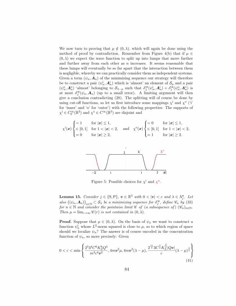
We now turn to proving that µ /∈ (0, λ), which will again be done using themethod of proof by contradiction. Remember from Figure 4(b) that if µ ∈(0, λ) we expect the wave function to split up into lumps that move furtherand further away from each other as n increases. It seems reasonable thatthese lumps will eventually be so far apart that the interaction between themis negligible, whereby we can practically consider them as independent systems.Given a term (ψn,An) of the minimizing sequence our strategy will thereforebe to construct a pair (ψi

n,Ain) which is ‘almost’ an element of Sµ and a pair

(ψon,A

on) ‘almost’ belonging to Sλ−µ such that E v

j (ψin,A

in) + E v

j (ψon,A

on) is

at most E vj (ψn,An) (up to a small error). A limiting argument will then

give a conclusion contradicting (28). The splitting will of course be done byusing cut-off functions, so let us first introduce some mappings χi and χo (‘i’for ‘inner’ and ‘o’ for ‘outer’) with the following properties: The supports ofχi ∈ C∞0 (R3) and χo ∈ C∞(R3) are disjoint and

χi(x)

= 1 for |x| ≤ 1,

∈ [0, 1] for 1 < |x| < 2,

= 0 for |x| ≥ 2,

and χo(x)

= 0 for |x| ≤ 1,

∈ [0, 1] for 1 < |x| < 2,

= 1 for |x| ≥ 2.

Figure 5: Possible choices for χi and χo.

Lemma 15. Consider j ∈ S,P, v ∈ R3 with 0 < |v| < c and λ ∈ Λvj . Let

also((ψn,An)

)n∈N ⊂ Sλ be a minimizing sequence for E v

j , define Cn by (33)for n ∈ N and consider the pointwise limit C of (a subsequence of ) (Cn)n∈N.Then µ = limr→∞ C (r) is not contained in (0, λ).

Proof. Suppose that µ ∈ (0, λ). On the basis of ψn we want to construct afunction ψi

n whose L2-norm squared is close to µ, so to which region of spaceshould we localize ψn? The answer is of course encoded in the concentrationfunction of ψn, so more precisely: Given

0 < ε < min

2534C6K6SQ

4

m3c4v2, 4mv2µ, 4mv2(λ− µ),

2114 3C

32K

32S |Qv|

c(λ− µ)

34

(41)

84

we choose (by the definition of µ) a number

R > max

2

32~√

λ

εm‖∇χ`‖L∞ ,

16C~λ12

εm‖∇χ`‖L∞

∣∣∣∣∣ ` ∈ i, o

∨ 2234K2SC

2Q2λ2v2

ε2√πc2

(max

∥∥∇χi∥∥L12 ,

∥∥∇χo∥∥L3

)2 (42)

such that µ− ε4/3c4/3

211/334/3C2K2S |Qv|4/3 < C (R). As a first step we will consider n’s

so large that

µ− ε43 c

43

2113 3

43C2K2

S |Qv|43

< Cn(R) < µ+ε

43 c

43

2113 3

43C2K2

S |Qv|43

. (43)

Here, the upper bound on Cn(R) is strictly speaking redundant, since we willlater obtain a better upper bound by considering even larger values of n – butalready at this point it is advantageous to think of Cn(R) as being close to µ.We should not just perceive Cn(R) as being an abstract supremum – it is infact the probability mass of the particle in the vicinity of some point in space.Because ψn ∈ L2 the continuous function y 7→

∫B(y,R) |ψn(x)|2 dx will namely

approach zero as |y| → ∞, whereby we can choose a point yn ∈ R3 such that

Cn(R) =

∫

B(yn,R)|ψn(x)|2 dx. (44)

So in the ball B(yn, R) we have found a ψn-lump whose probability mass isessentially µ. The other lumps are expected to move away as n increases, so forlarge n there should be a large area around B(yn, R) where ψn has essentiallyno probability mass. As a consequence we can construct the function ψo

n bycutting away the values of ψn on a ball centered at yn with quite a large radius.It turns out that we can in fact choose this radius on the form 2knR, wherethe sequence (kn)n∈N of integers satisfies

(I) kn →∞ for n→∞,

(II) Cn(2knR) ≤ µ+ ε4/3c4/3

211/334/3C2K2S |Qv|4/3 for all n ∈ N.

One can namely easily verify that the sequence of numbers

kn =

log2

sup C−1n

((0, µ+ ε4/3c4/3

211/334/3C2K2S |Qv|4/3

])

2R

has the desired properties, where b·c denotes the floor function and log2 denotesthe binary logarithm2. Thus, we will construct ψi

n and ψon by multiplication

2The floor function is x 7→ maxm ∈ Z | m ≤ x and the binary logarithm is x 7→ log(x)log(2)

,where log denotes the natural logarithm.

85

with the cut-off functions given by

χi,ψn (x) = χi

(x− ynR

)respectively χo,ψ

n (x) = χo( x− yn

2kn−1R

)

for x ∈ R3. Let us emphasize that we use the superscript ψ because thesefunctions will be used to cut the wave function ψ into the two pieces ψi

n andψon – later we will define corresponding cut-off functions χi,A

n and χo,An to cut

A into two pieces Ain and Ao

n.Let us now do this splitting of the An-field into Ai

n- and Aon-fields. We will

aim to make the cuts in the big gap between B(yn, 2R) and R3\B(yn, 2kn−1R),

where the functions ψin and ψo

n are guaranteed to vanish. So we decomposespace into the disjoint union R3 = B(yn, R) ∪

(⋃∞m=1Amn

), where

Amn =x ∈ R3

∣∣ 2m−1R ≤ |x− yn| < 2mR

for m ∈ N (see Figure 6).

Figure 6: The two-dimensional analogues of the spherical shells A0n,A1

n, . . ..

By point (I) from above we have kn ≥ 4 for n sufficiently large and for such n’sthere must exist a numbermn in the set 2, . . . , kn−2 such that the inequality∥∥1Amnn An

∥∥6

L6 ≤ (kn − 3)−1∥∥1A2

n∪···∪Akn−2n

An

∥∥6

L6 holds true, whereby we havefor n sufficiently large that∥∥1Amnn An

∥∥L6

< min 1

4‖∇χ`‖L3

(√C2 +

επc2

c2 + v2− C

),

1

2‖∇χ`‖L3

√επc2

c2 + v2

∣∣∣` ∈ i, o.

(45)

In this way we can control An on Amnn , so we will define Ain and Ao

n using thecut-off functions

χi,An (x) = χi

( x− yn2mn−1R

)and χo,A

n (x) = χo( x− yn

2mn−1R

).

More precisely, we will for ` ∈ i, o introduce the mapping u`n : R3 → R

86

Figure 7: The distance to yn is measured along the first axis.

given by

u`n(x) =1

4π

∫

R3

1

|x− y|div(χ`,An An

)(y) dy for almost every x ∈ R3

and define ψin, ψo

n, Ain and Ao

n by

ψ`n = eiQ~c u

`nχ`,ψn ψn and A`

n = χ`,An An +∇u`n.

We observe that div(χ`,An An

)= ∇χ`,An ·An is contained inH1 and has compact

support so from Lemma 19 we obtain that ψ`n ∈ H1, A`n ∈ D1 with divA`

n = 0and

∇u`n(x) = − 1

4π

∫

R3

x− y|x− y|3 div

(χ`,An An

)(y) dy for almost every x ∈ R3.

(46)

Moreover, ψin and ψo

n satisfy

max

∣∣∣∣µ−∫

R3

|ψin(x)|2 dx

∣∣∣∣ ,∣∣∣∣λ− µ−

∫

R3

|ψon(x)|2 dx

∣∣∣∣<

ε43 c

43

2113 3

43C2K2

S |Qv|43

.

(47)

which follows from (43), (II) as well as the estimates

Cn(R) ≤∫

R3

|ψin(x)|2 dx ≤

∫

B(yn,2R)|ψn(x)|2 dx ≤ Cn(2R) ≤ Cn(2knR)

and

Cn(R) ≤ λ−∫

R3

|ψon(x)|2 dx ≤

∫

B(yn,2knR)|ψn(x)|2 dx ≤ Cn(2knR).

In the motivational remarks made above Lemma 15 we mentioned the desireto construct ψ`n and A`

n in such a way that they ‘almost’ satisfy(ψin,A

in

)∈ Sµ

and(ψon,A

on

)∈ Sλ−µ. The precise meaning of this informal statement is that

the pairs(ψ`n,A

`n

)∈ H1 ×D1 have the properties divA`

n = 0 and (47).

87

The next step in our argument is to show that

E vj (ψn,An) ≥ E v

j (ψin,A

in) + E v

j (ψon,A

on)− ε. (48)

We begin by estimating the 12m‖∇j,An+mc

Qvψn‖2L2-term on the right hand side

of (16). For this we observe that χ`,An χ`,ψn = χ`,ψn , whereby we can rewrite

e−iQ~c u

`n∇j,A`

n+mcQ

vψ`n = ∇j,0χ`,ψn ψn + χ`,ψn ∇j,An+mc

Qvψn,

which allows us to apply (15), (42) and Remark 12 to obtain

‖∇j,A`n+mc

Qvψ

`n‖2L2

≤ ~2λ

R2‖∇χ`‖2L∞ + ‖χ`,ψn ∇j,An+mc

Qvψn‖2L2 +

2C~λ12

R‖∇χ`‖L∞

≤ ‖χ`,ψn ∇j,An+mcQ

vψn‖2L2 +εm

4.

and consequently1

2m‖∇j,An+mc

Qvψn‖2L2 ≥

1

2m

∑

`∈i,o‖∇j,A`

n+mcQ

vψ`n‖2L2 −

ε

4. (49)

To treat the term −Qc (ψn,v ·Anψn)L2 appearing on the right hand side of (16)

we establish two auxiliary estimates: The first estimate∣∣∣∫

R3

v ·An

(|ψn|2 − |ψi

n|2 − |ψon|2)

dx∣∣∣

≤ |v|‖An‖L6

∥∥∥∥√

1− (χi,ψn )2 − (χo,ψ

n )2ψn

∥∥∥∥12

L6

(∫

R3

(|ψn|2 − |ψi

n|2 − |ψon|2)

dx) 3

4

≤ εc

12|Q|follows from (47), Hölder’s and Sobolev’s inequalities. By choosing n largeenough we previously made sure that kn ≥ 4 and 2 ≤ mn ≤ kn − 2 whereby(46), the Hölder inequality and (42) yield the second auxiliary estimate∣∣∣∫

R3

v · ∇u`n|ψ`n|2 dx∣∣∣

≤ |v|4π

∫

R3

∫

Amnn

1

|x− y|2 |∇χ`,An (y)||An(y)| dy |ψ`n(x)|2 dx

≤

|v|4π

∥∥∥∥1B(0,(2+2mn )R)1

| · |

∥∥∥∥2

L83

‖∇χi,An ‖L12‖An‖L6‖ψi

n‖2L2 for ` = i

|v|4π

∥∥∥∥1R3\B(0,(2kn−1−2mn )R)

1

| · |

∥∥∥∥2

L4

‖∇χo,An ‖L3‖An‖L6‖ψo

n‖2L2 for ` = o

≤ 3|v|KSCλ

2π14R

12

max‖∇χi‖L12 , ‖∇χo‖L3

<εc

12|Q| .

88

By combining the two previous estimates with the identity χ`,An χ`,ψn = χ`,ψn weobtain

|(ψn,v ·Anψn)L2 − (ψin,v ·Ai

nψin)L2 − (ψo

n,v ·Aonψ

on)L2 |

=∣∣∣∫

R3

v ·An

(|ψn|2 − |ψi

n|2 − |ψon|2)

dx−∑

`∈i,o

∫

R3

v · ∇u`n|ψ`n|2 dx∣∣∣

<εc

4|Q| . (50)

Finally, we estimate the 18π

(‖∇⊗An‖2L2 −

∥∥(vc · ∇

)An

∥∥2

L2

)-term on the right

hand side of (16) by noting that

‖∇ ⊗An‖2L2 −∥∥∥(vc· ∇)An

∥∥∥2

L2

≥∑

`∈i,o

(‖χ`,An ∇⊗An‖2L2 −

∥∥∥χ`,An(vc· ∇)An

∥∥∥2

L2

)

≥∑

`∈i,o

(‖∇ ⊗A`

n‖2L2 −∥∥∥(vc· ∇)A`n

∥∥∥2

L2

− 2(

1 +v2

c2

)‖∇ ⊗A`

n‖L2

(‖∇χ`,An ⊗An‖L2 + ‖∇ ⊗∇u`n‖L2

)

− 2(

1 +v2

c2

)‖∇χ`,An ⊗An‖L2‖∇ ⊗∇u`n‖L2

),

(51)

where we at the second step use the identities

χ`,An ∇⊗An = ∇⊗A`n − (∇χ`,An ⊗An +∇⊗∇u`n), (52)

χ`,An

(vc· ∇)An =

(vc· ∇)A`n −

((vc· ∇)χ`,An An +

(vc· ∇)∇u`n

)

and the nonnegativity of(1− v2

c2

)(‖∇χ`,An ⊗An‖2 + ‖∇⊗∇u`n‖2L2). As can be

seen by approximating ∇u`n in D1 by C∞0 -functions, applying the Planchereltheorem and using the general vector identity |F |2|G|2 = |F ·G|2 + |F ×G|2we have ‖∇ ⊗ ∇u`n‖2L2 = ‖div∇u`n‖2L2 + ‖∇ × ∇u`n‖2L2 = ‖∇χ`,An · An‖2L2 .Consequently, ‖∇ ⊗ ∇u`n‖L2 and ‖∇χ`,An · An‖L2 have the common upperbound ‖∇χ`‖L3

∥∥1Amnn An

∥∥L6 that is small by (45). Moreover, ‖∇ ⊗A`

n‖L2 isaccording to (52) bounded from above by C + 2‖∇χ`‖L3

∥∥1Amnn An

∥∥L6 and so

we can use (45) to continue (51) and get

1

8π

(‖∇ ⊗An‖2L2 −

∥∥∥(vc· ∇)An

∥∥∥2

L2

)

≥∑

`∈i,o

1

8π

(‖∇ ⊗A`

n‖2L2 −∥∥∥(vc· ∇)A`n

∥∥∥2

L2

)− ε

4. (53)

89

Now, (48) is an immediate consequence of (49), (50), (53) and the inequality

max

∣∣∣∣µ−∫

R3

|ψin(x)|2 dx

∣∣∣∣ ,∣∣∣∣λ− µ−

∫

R3

|ψon(x)|2 dx

∣∣∣∣<

ε

4mv2(54)

that follows from (41) and (47).Finally, Remark 8 and (54) give

E vj (ψn,An) ≥ I‖ψ

in‖2L2

j + I‖ψon‖2L2

j − ε ≥ Iµ+ ε4mv2

j + Iλ−µ+ ε

4mv2

j − ε,

so letting n diverge to infinity produces the estimate

Iλj ≥ Iµ+ ε

4mv2

j + Iλ−µ+ ε

4mv2

j − ε.

By Lemma 9 we can therefore take the limit ε→ 0+ and obtain the inequalityIλj ≥ Iµj + Iλ−µj contradicting (28).

Combining the Lemmas 14 and 15 allows us to reach the conclusion thatlimr→∞ C (r) is equal to λ. This is exactly what we need to break the trans-lation invariance of our problem.

Proposition 16. Given j ∈ S,P, v ∈ R3 with 0 < |v| < c and λ ∈ Λvj

consider a minimizing sequence((ψn,An)

)n∈N ⊂ Sλ for E v

j . Then there existsa sequence (yn)n∈N of points in R3 with the following property: For every ε > 0there exists an R > 0 such that for all n ∈ N

∥∥1B(yn,R)ψn∥∥2

L2 ≥ λ− ε.

This property is sometimes expressed by saying that the maps x 7→ |ψn(x+yn)|2are tight.

Proof. Given ν > 0 we will first argue that it is possible to find an rν > 0such that

Cn(rν) > λ− ν for all n ∈ N. (55)

By the identity limr→∞ C (r) = λ we can namely consider a ρ > 0 such thatC (ρ) > λ− ν and then we can choose an N ∈ N such that Cn(ρ) > λ− ν forn > N , simply because limn→∞ Cn(ρ) = C (ρ). Finally, we can use the factthat limr→∞ Cn(r) = λ for each of the finitely many n’s in the set 1, . . . , Nto find a ρn > 0 satisfying Cn(ρn) > λ−ν. Then because Cn is a nondecreasingfunction the inequality (55) holds true with rν = maxρ, ρ1, . . . , ρN.

Now, the definition of Cn(rν) guarantees the existence of a sequence (yνn)n∈Nof points in R3 satisfying

∥∥1B(yνn,rν)ψn

∥∥2

L2 > λ− ν for all n ∈ N.

90

Figure 8: By setting R = rλ2 + 2rε we get that B(yεn, r

ε) ⊂ B(yn, R) becausethe balls B(yn, r

λ2 ) and B(yεn, r

ε) are guaranteed not to be disjoint.

Our aim will be to prove that by setting yn = yλ2n for n ∈ N we obtain a

sequence (yn)n∈N with properties as stated in the proposition. To achieve thisgoal consider an arbitrary ε in the interval

(0, λ2

). Then for every n ∈ N both of

the integrals∫B(yn,rλ/2) |ψn(x)|2 dx and

∫B(yεn,r

ε) |ψn(x)|2 dx must be strictlylarger than λ

2 , which together with the fact that∫R3 |ψn(x)|2 dx = λ gives that

the balls B(yn, rλ2 ) and B(yεn, r

ε) have a nonempty intersection. This enablesus to define R = r

λ2 + 2rε and thereby obtain∥∥1B(yn,R)ψn

∥∥2

L2 ≥∥∥1B(yεn,r

ε)ψn∥∥2

L2 > λ− ε,

for any n ∈ N, which is the desired result.

5.2 The Lower Semicontinuity Argument

We began by considering an arbitrary minimizing sequence((ψn,An)

)n∈N for

E vj . As we will see below our efforts in the previous section enable us to apply

the direct method in the calculus of variations to the sequence of translatedpairs

(ψ′n,A′n) = (ψn τyn ,An τyn),

where (yn)n∈N denotes the sequence whose existence is guaranteed in Propo-sition 16. Due to E v

j ’s translation invariance((ψ′n,A

′n))n∈N will namely be a

minimizing sequence for E vj and by Proposition 16 we have

∀ε > 0 ∃R > 0∀n ∈ N :∥∥1B(0,R)ψ

′n

∥∥2

L2 =∥∥1B(yn,R)ψn

∥∥2

L2 ≥ λ− ε. (56)

This enables us to show the existence of a minimizer for E vj on Sλ.

Theorem 17. For every choice of j ∈ S,P, v ∈ R3 with 0 < |v| < c andλ ∈ Λv

j there exists a pair (ψ,A) ∈ Sλ such that E vj (ψ,A) = Iλj .

91

Proof. According to Lemma 11 (together with the Sobolev inequality) thesequences (ψ′n)n∈N, (A′n)n∈N and (∇ ⊗ A′n)n∈N are bounded in the reflexiveBanach spaces H1, L6 respectively L2. Thus, the Banach-Alaoglu theoremgives the existence of functions ψ ∈ H1 and A ∈ L6 with square integrablederivatives such that (passing to subsequences)

ψ′n −−−n→∞ψ in H1, A′n −−−n→∞

A in L6 and ∂`A′n −−−n→∞

∂`A in L2 (57)

for ` ∈ 1, 2, 3. Observe that we can (after passing to yet another subse-quence) assume that

ψ′n −−−→n→∞ψ and A′n −−−→n→∞

A pointwise almost everywhere in R3 (58)

as a consequence of (57) and the result [11, Corollary 8.7] about weak conver-gence implying a.e. convergence of a subsequence.

The pair (ψ,A) is our candidate for a minimizer, so we begin by showingthat (ψ,A) ∈ Sλ. In this context the only nontrivial condition to check isthat the identity ‖ψ‖2L2 = λ holds true. The inequality ‖ψ‖2L2 ≤ λ followsimmediately from (57) and weak lower semicontinuity of the norm ‖ · ‖L2 (asexpressed in [11, Theorem 2.11]). To prove the opposite inequality we let ε > 0be given and use (56) to choose an R > 0 such that

∥∥1B(0,R)ψ′n

∥∥2

L2 ≥ λ− ε for all n ∈ N. (59)

By (57) and the Rellich-Kondrashov theorem [11, Theorem 8.6] the left handside of (59) converges to

∥∥1B(0,R)ψ∥∥2

L2 as n tends to infinity. Hence we have‖ψ‖2L2 ≥ λ− ε for any ε > 0 and consequently ‖ψ‖2L2 ≥ λ. Besides giving thedesired conclusion that (ψ,A) ∈ Sλ this also enables us to deduce that

ψ′n −−−→n→∞ψ in L2, (60)

simply because the recently gained knowledge that ‖ψ‖2L2 = ‖ψ′n‖2L2 = λ givestogether with (57) that

‖ψ − ψ′n‖2L2 = ‖ψ‖2L2 + ‖ψ′n‖2L2 − 2Re(ψ,ψ′n

)L2 −−−→

n→∞0.

Finally, we observe that by (58) the sequence ((A′n)`ψ′n)n∈N converges point-wise almost everywhere to A`ψ and by the Hölder inequality it is bounded byK

32SC

32λ

14 in L2 for each ` ∈ 1, 2, 3. We now use that a bounded sequence

of functions converging pointwise a.e. to some L2-limit also converges weaklyin L2 to the same limit – to prove the weak convergence it suffices namely totest against C∞0 -functions by [19, Theorem V.1.3] and thus the result followsfrom Egorov’s theorem [19, Section 0.3]. This yields

(A′n)`ψ′n −−−n→∞A`ψ in L2,

92

which together with (57) implies that

∇j,A′nψ′n −−−n→∞∇j,Aψ in L2. (61)

The remaining task to overcome is proving that Iλj = E vj (ψ,A) – or rather

that Iλj ≥ E vj (ψ,A) since the opposite inequality is trivially true. By super-

additivity of lim inf and (12) we get

Iλj ≥1

2mlim infn→∞

‖∇j,A′nψ′n‖2L2 + ~ lim infn→∞

(ψ′n, iv · ∇ψ′n)L2

+1

8πlim infn→∞

(‖∇ ⊗A′n‖2L2 −

∥∥∥(vc· ∇)A′n∥∥∥

2

L2

), (62)

so we will have to estimate each of the terms on the right hand side of (62).That

lim infn→∞

‖∇j,A′nψ′n‖2L2 ≥ ‖∇j,Aψ‖2L2 (63)

follows immediately from (61) and the weak lower semicontinuity of ‖ · ‖L2 .Using (60), (57) and Lemma 11 gives

∣∣(ψ′n, iv · ∇ψ′n)L2 − (ψ, iv · ∇ψ)L2

∣∣

≤ |v|C‖ψ′n − ψ‖L2 +3∑

`=1

|v`||(ψ, ∂`ψ′n − ∂`ψ)L2 |

−−−→n→∞

0

and therefore

lim infn→∞

(ψ′n, iv · ∇ψ′n)L2 = (ψ, iv · ∇ψ)L2 . (64)

To treat the last term on the right hand side of (62) we imagine that v pointsin the direction of the first axis, whereby the functional

H : D1 3 B 7→√‖∇ ⊗B‖2

L2 −∥∥∥(vc· ∇)B∥∥∥

2

L2∈ R

simply reduces to

H (B) =

∥∥∥∥∥∥∥

√1− v2

c2∂1

∂2

∂3

⊗B

∥∥∥∥∥∥∥L2

.

It is immediately apparent that H is a convex functional (by the triangleinequality) and H is continuous D1 → R since H (B) ≤ ‖∇ ⊗B‖L2 for all

93

B ∈ D1. Therefore we get from Mazur’s theorem [4, Corollary 3.9] that H isweakly lower semicontinuous, which together with (57) implies that

lim infn→∞

(‖∇ ⊗A′n‖2L2 −

∥∥∥(vc· ∇)A′n∥∥∥

2

L2

)≥ ‖∇⊗A‖2L2 −

∥∥∥(vc· ∇)A∥∥∥

2

L2,

(65)

since weak convergence of a sequence (fn)n∈N to some function f in the Hilbertspace D1 by the Riesz representation theorem is characterized by the limit(∇fn,∇g

)L2 −−−→

n→∞(∇f,∇g

)L2 holding true for every choice g ∈ D1. Finally,

combining (62), (63), (64) and (65) results in the inequality Iλj ≥ E vj (ψ,A).

Combining Theorem 17 with Lemma 3 now gives the main result.

6 Behavior of the Energy for small velocities of the Particle

In this final section we estimate the energy of our travelling wave solutions.The next Theorem 18 shows that to leading order for small |v| the energybehaves like mv2

2 λ. We interpret this as saying that there is no change ineffective mass due to the electromagnetic field.

Theorem 18. Let j ∈ S,P and λ > 0 be given. Then there exist θj , κj > 0(only depending on j, λ, ~, c,Q and m) such that

∣∣∣Ej(v, ψ,A)− mv2

2λ∣∣∣ ≤ κj |v|3

for any v ∈ R3 with 0 < |v| < θj and any minimizer (ψ,A) of E vj on Sλ.

Proof. Let j ∈ S,P, λ > 0 as well as v ∈ R3 with 0 < |v| < Θλj,+ be given

and consider an arbitrary minimizer (ψ,A) of E vj on Sλ. Then according to

Lemma 6 and (26) the pair (ψ,A) must satisfy (19). Thereby (24), (25) andLemma 6 give that

‖ψ‖2L6 ≤26π2K8

SQ4m2λ3

~4

v4

(Θλj,+ − |v|)2(|v| −Θλ

j,−)2

and

‖∇ ⊗A‖2L2 ≤28π3K6

Sc2Q4mλ3

~2

v4

(c2 − v2)2(Θλj,+ − |v|)(|v| −Θλ

j,−).

Using these estimates together with (16), Lemma 6, Hölder’s and Sobolev’sinequalities results in the inequality

‖∇j,A+mcQ

vψ‖2L2 ≤26π2K6

SQ4m2λ3

~2

v4(c2(1 +√

2)

+ v2(1−√

2))

(c2 − v2)2(Θλj,+ − |v|)(|v| −Θλ

j,−)

94

and so the desired result follows immediately from the identities

ES(v, ψ,A) =1

2m‖∇S,A+mc

Qvψ‖2L2 +

mv2

2λ− (ψ,v · ∇S,A+mc

Qvψ)L2

+1

8π

∫

R3

(∣∣∣(vc· ∇)A∣∣∣2

+ |∇ ×A|2)

dxλ

and

EP(v, ψ,A) =1

2m‖∇P,A+mc

Qvψ‖2L2 +

mv2

2λ− Re(σ · vψ,∇P,A+mc

Qvψ)L2

+1

8π

∫

R3

(∣∣∣(vc· ∇)A∣∣∣2

+ |∇ ×A|2)

dxλ.

A The Poisson Equation

Given some function f the corresponding Poisson equation reads

−∆u = f. (66)

Let us briefly recall the contents of [11, Theorem 6.21] and [11, Remark6.21(2)]: If

f ∈ L1loc(R3) and

∫

R3

|f(y)|1 + |y| dy <∞ (67)

then defining u : R3 → C by

u(x) =1

4π

∫

R3

1

|x− y|f(y) dy (68)

for almost every x ∈ R3 results in a locally integrable solution of (66). More-over, the distributional gradient ∇u can be identified with the function givenby

∇u(x) = − 1

4π

∫

R3

x− y|x− y|3 f(y) dy (69)

for almost every x ∈ R3. We will need the following result.

Lemma 19. If f ∈ L1 ∩ L3 and ∇f ∈ L1 ∩ L 54 then u defined by (68) is a

D1-function solving (66) in the distribution sense. Likewise, if f ∈ H1 hascompact support then u solves (66) and ∇u ∈ D1.

Proof. Verifying the condition (67) in each of the two scenarios outlined inthe statement of the lemma is an easy task, which is left for the reader – in thiscontext it is useful to note that y 7→ 1

1+|y| is e.g. an L6-function. Thus, the

95

function defined almost everywhere by (68) is indeed a solution of the Poissonequation in those two cases.

Suppose that f ∈ L1 ∩ L3 and ∇f ∈ L1 ∩ L 54 . Then we first show that u

vanishes at infinity: For this let N denote the null set on which the identities(68) and (69) do not hold true. Then for each sequence (xk)k∈N of elementsin R3 \ N with |xk| −−−→

k→∞∞ we have

|u(xk)| ≤1

4π

∥∥1B(xk,1)f∥∥L3

∥∥∥∥1B(0,1)

| · |

∥∥∥∥L

32

+1

4π

∥∥∥∥(1R3\B(xk,1)f)(·)|xk − · |

∥∥∥∥L1

−−−→k→∞

0,

where we split the integral involved in the expression for u(xk) into a contri-bution from B(xk, 1) as well as a contribution from R3 \ B(xk, 1) and treatthese by means of the Hölder inequality and Lebesgue’s dominated conver-gence theorem. In order to prove that ∇u is square integrable we use theHölder inequality and Tonelli’s theorem to get∫

R3

|∇u(x)|2 dx

≤ 1

8π2

∫

R3

(∫

B(x,1)

|f(y)||x− y|2 dy

)2dx+

1

8π2

∫

R3

(∫

R3\B(x,1)

|f(y)||x− y|2 dy

)2dx

≤ 1

8π2

∫

R3

∫

B(x,1)

|f(y)||x− y| 52

dy dx

∥∥∥∥1B(0,1)

| · |

∥∥∥∥32

L52

‖f‖110

L1‖f‖910

L3

+1

8π2

∫

R3

∫

R3\B(x,1)

|f(y)||x− y| 72

dy dx

∥∥∥∥1R3\B(0,1)

| · |

∥∥∥∥12

L72

‖f‖314

L3‖f‖1114

L1

≤ 1

8π2

∥∥∥∥1B(0,1)

| · |

∥∥∥∥4

L52

‖f‖1110

L1‖f‖910

L3 +1

8π2

∥∥∥∥1R3\B(0,1)

| · |

∥∥∥∥4

L72

‖f‖314

L3‖f‖2514

L1

and so we conclude that u ∈ D1.Assume now that f ∈ H1 has support in some ball B(0, rf ). Then for all

x ∈ R3 \ N with |x| > rf we have

|∇u(x)| ≤ 1

4π(|x| − rf )2

(4

3πr3

f

) 12 ‖f‖L2

whereby we deduce that ∇u vanishes at infinity. Combining the change ofvariables z = x−y with a naive differentiation under the integral sign in (69)suggests that

∂j∂ku(x) = − 1

4π

∫

R3

xk − yk|x− y|3∂jf(y) dy (70)

for j, k ∈ 1, 2, 3 and almost every x ∈ R3. Under the assumption that f hassquare integrable first derivatives and compact support, the right hand side of

96

(a) |x− y| < 3rf (b) |x− y| > rf

Figure 9: Estimates on the distance from x to any y ∈ suppf ⊂ B(0, rf ) inthe cases x ∈ B(0, 2rf ) respectively x ∈ R3 \ B(0, 2rf ). Both estimates followfrom the triangle inequality in R3.

(70) is indeed well defined almost everywhere in R3: The function y 7→ |∂jf(y)||x−y|2

(and thereby also y 7→ xk−yk|x−y|3∂jf(y)) must namely be integrable for almost all

x ∈ B(0, 2rf ), since Tonelli’s theorem, the Cauchy-Schwarz inequality and thebasic observation stated on Figure 9(a) give that

∫

B(0,2rf )

∫

B(0,rf )

|∂jf(y)||x− y|2 dy dx ≤

(4

3πr3

f

) 12

∥∥∥∥1B(0,3rf )1

| · |

∥∥∥∥2

L2

‖∂jf‖L2 . (71)

On the other hand y 7→ |∂jf(y)||x−y|2 is majorized by the integrable function |∂jf |

r2f

for all x ∈ R3 \ B(0, 2rf ), as shown on Figure 9(b). Thus, it makes sense toconsider the function given (a.e.) by the expression on the right hand sideof (70) – the identification of this function with the distribution ∂j∂ku thenfollows from a standard argument utilizing Fubini’s theorem (which is outlinedin the proof of [11, Theorem 6.21]). It just remains to be proven that thefunctions ∂j∂ku are square integrable – we first verify this square integrabilityon the ball B(0, 2rf ). This is done by using the Hölder inequality, the Jenseninequality and the Hardy-Littlewood-Sobolev inequality:

∫

B(0,2rf )|∂j∂ku(x)|2 dx

≤ 1

16π2

∫

B(0,2rf )

(∫

B(0,rf )

|∂jf(y)| 65|x− y| 94

dy) 10

9(∫ 1B(0,3rf )(x− y)

|x− y| 2710dy) 5

9‖∂jf‖23

L2dx

≤(

43πr

3f

) 19

16π2

∫

B(0,2rf )

∫

B(0,rf )

|∂jf(y)| 43|x− y| 52

dy dx

∥∥∥∥1B(0,3rf )1

| · |

∥∥∥∥32

L2710

‖∂jf‖23

L2

≤(

43πr

3f

) 19

8π2

(4

3π) 5

6((5

3

) 56

+(5

2

) 56)(4

3π(2rf )3

) 12

∥∥∥∥1B(0,3rf )1

| · |

∥∥∥∥32

L2710

‖∂jf‖2L2 .

97

Finally, the Cauchy-Schwarz inequality, Tonelli’s theorem and the observationon Figure 9(b) give

∫

R3\B(0,2rf )|∂j∂ku(x)|2 dx ≤ 1

16π2

(4

3πr3

f

)∥∥∥∥1R3\B(0,rf )1

| · |

∥∥∥∥4

L4

‖∂jf‖2L2 ,

whereby ∂j∂ku is also square integrable on R3 \ B(0, 2rf ). Consequently, ∇uis a D1-function.

Remark 20. Consider a locally integrable, harmonic function u with squareintegrable first derivatives. The harmonicity of ∇u ensures the existence ofvector fields pm on R3 with homogeneous harmonic polynomials of degree mas coordinates such that

∇u(x) =

∞∑

m=0

pm(x)

for all x ∈ R3 (see [1, Corollary 5.34 and Proposition 1.30]). The serieseven converges absolutely and uniformly on compact subsets of R3 so for anarbitrary given R > 0 we have the series representation ∇u =

∑∞m=0 pm in[

L2(B(0, R)

)]3. Integrating in polar coordinates and using the homogeneity ofthe functions pm as well as the spherical harmonic decomposition [1, Theorem5.12] of L2(∂B(0, 1)) now gives

∥∥1B(0,R)∇u∥∥2

L2 =∞∑

m=0

∞∑

`=0

∫ R

0rm+`+2 dr

(pm,p`

)L2(∂B(0,1))

=∞∑

m=0

R2m+3

2m+ 3‖pm‖2L2(∂B(0,1)). (72)

By Lebesgue’s dominated convergence theorem the left hand side of (72) con-verges to ‖∇u‖2L2 as R→∞ so the same must be true for the right hand side.But the right hand side simply can not converge as R→∞ unless pm ≡ 0 forall m ∈ N0 – so we conclude that ∇u ≡ 0. Therefore u is a constant function –consequently, the Poisson equation can at most have one solution in the spaceD1.

References

[1] Sheldon Axler, Paul Bourdon, and Wade Ramey. Harmonic functiontheory, volume 137 of Graduate Texts in Mathematics. Springer-Verlag,New York, second edition, 2001.

[2] Ioan Bejenaru and Daniel Tataru. Global wellposedness in the en-ergy space for the Maxwell-Schrödinger system. Comm. Math. Phys.,288(1):145–198, 2009.

98

[3] Vieri Benci and Donato Fortunato. An eigenvalue problem forthe Schrödinger-Maxwell equations. Topol. Methods Nonlinear Anal.,11(2):283–293, 1998.

[4] Haim Brezis. Functional analysis, Sobolev spaces and partial differentialequations. Universitext. Springer, New York, 2011.

[5] B. Buffoni, M. D. Groves, S. M. Sun, and E. Wahlén. Existence andconditional energetic stability of three-dimensional fully localised solitarygravity-capillary water waves. J. Differential Equations, 254(3):1006–1096, 2013.

[6] Giuseppe Maria Coclite and Vladimir Georgiev. Solitary waves forMaxwell-Schrödinger equations. Electron. J. Differential Equations, pagesNo. 94, 31 pp. (electronic), 2004.

[7] Maria J. Esteban, Vladimir Georgiev, and Eric Séré. Stationary solutionsof the Maxwell-Dirac and the Klein-Gordon-Dirac equations. Calc. Var.Partial Differential Equations, 4(3):265–281, 1996.

[8] Jürg Fröhlich, B. Lars G. Jonsson, and Enno Lenzmann. Boson stars assolitary waves. Comm. Math. Phys., 274(1):1–30, 2007.

[9] Yan Guo, Kuniaki Nakamitsu, and Walter Strauss. Global finite-energysolutions of the Maxwell-Schrödinger system. Comm. Math. Phys.,170(1):181–196, 1995.

[10] A. N. Kolmogorov and S. V. Fomin. Introductory real analysis. RevisedEnglish edition. Translated from the Russian and edited by Richard A.Silverman. Prentice-Hall Inc., Englewood Cliffs, N.Y., 1970.

[11] Elliott H. Lieb and Michael Loss. Analysis, volume 14 of Graduate Studiesin Mathematics. American Mathematical Society, Providence, RI, secondedition, 2001.

[12] P.-L. Lions. The concentration-compactness principle in the calculus ofvariations. The locally compact case. I. Ann. Inst. H. Poincaré Anal. NonLinéaire, 1(2):109–145, 1984.

[13] P.-L. Lions. The concentration-compactness principle in the calculus ofvariations. The locally compact case. II. Ann. Inst. H. Poincaré Anal.Non Linéaire, 1(4):223–283, 1984.

[14] S. G. Mihlin. On the multipliers of Fourier integrals. Dokl. Akad. NaukSSSR (N.S.), 109:701–703, 1956.

[15] Kuniaki Nakamitsu and Masayoshi Tsutsumi. The Cauchy problem for thecoupled Maxwell-Schrödinger equations. J. Math. Phys., 27(1):211–216,1986.

99

[16] Makoto Nakamura and Takeshi Wada. Global existence and uniquenessof solutions to the Maxwell-Schrödinger equations. Comm. Math. Phys.,276(2):315–339, 2007.

[17] Kim Petersen. The Mathematics of Charged Particles interacting withElectromagnetic Fields. 2013.

[18] Kim Petersen. Existence of a Unique Local Solution to the Many-bodyMaxwell-Schrödinger Initial Value Problem. Preprint 2013.

[19] Kôsaku Yosida. Functional analysis, volume 123 ofGrundlehren der Math-ematischen Wissenschaften [Fundamental Principles of Mathematical Sci-ences]. Springer-Verlag, Berlin, sixth edition, 1980.

100