Phased LSTM: Accelerating Recurrent NetworkTraining for Long or Event-based Sequences

Daniel Neil, Michael Pfeiffer, and Shih-Chii LiuInstitute of Neuroinformatics

University of Zurich and ETH ZurichZurich, Switzerland 8057

{dneil, pfeiffer, shih}@ini.uzh.ch

Abstract

Recurrent Neural Networks (RNNs) have become the state-of-the-art choice forextracting patterns from temporal sequences. However, current RNN models areill-suited to process irregularly sampled data triggered by events generated incontinuous time by sensors or other neurons. Such data can occur, for example,when the input comes from novel event-driven artificial sensors that generatesparse, asynchronous streams of events or from multiple conventional sensors withdifferent update intervals. In this work, we introduce the Phased LSTM model,which extends the LSTM unit by adding a new time gate. This gate is controlledby a parametrized oscillation with a frequency range that produces updates of thememory cell only during a small percentage of the cycle. Even with the sparseupdates imposed by the oscillation, the Phased LSTM network achieves fasterconvergence than regular LSTMs on tasks which require learning of long sequences.The model naturally integrates inputs from sensors of arbitrary sampling rates,thereby opening new areas of investigation for processing asynchronous sensoryevents that carry timing information. It also greatly improves the performance ofLSTMs in standard RNN applications, and does so with an order-of-magnitudefewer computes at runtime.

1 Introduction

Interest in recurrent neural networks (RNNs) has greatly increased in recent years, since largertraining databases, more powerful computing resources, and better training algorithms have enabledbreakthroughs in both processing and modeling of temporal sequences. Applications include speechrecognition [13], natural language processing [1, 20], and attention-based models for structuredprediction [5, 29]. RNNs are attractive because they equip neural networks with memories, andthe introduction of gating units such as LSTM and GRU [16, 6] has greatly helped in making thelearning of these networks manageable. RNNs are typically modeled as discrete-time dynamicalsystems, thereby implicitly assuming a constant sampling rate of input signals, which also becomesthe update frequency of recurrent and feed-forward units. Although early work such as [25, 10, 4]has realized the resulting limitations and suggested continuous-time dynamical systems approachestowards RNNs, the great majority of modern RNN implementations uses fixed time steps.

Although fixed time steps are perfectly suitable for many RNN applications, there are severalimportant scenarios in which constant update rates impose constraints that affect the precision andefficiency of RNNs. Many real-world tasks for autonomous vehicles or robots need to integrate inputfrom a variety of sensors, e.g. for vision, audition, distance measurements, or gyroscopes. Each sensormay have its own data sampling rate, and short time steps are necessary to deal with sensors withhigh sampling frequencies. However, this leads to an unnecessarily higher computational load and

30th Conference on Neural Information Processing Systems (NIPS 2016), Barcelona, Spain.

InputGate

it ot

ft

xt xt

xt

xt ct ht

Forget Gate

Output Gate

(a)

xt

InputGate

ct

it ot

ft

xtxt

xt

ht

Forget Gate

OutputGate

ct~

t

kt

t

kt

(b)

Figure 1: Model architecture. (a) Standard LSTM model. (b) Phased LSTM model, with time gate ktcontrolled by timestamp t. In the Phased LSTM formulation, the cell value ct and the hidden outputht can only be updated during an “open” phase; otherwise, the previous values are maintained.

power consumption so that all units in the network can be updated with one time step. An interestingnew application area is processing of event-based sensors, which are data-driven, and record stimuluschanges in the world with short latencies and accurate timing. Processing the asynchronous outputs ofsuch sensors with time-stepped models would require high update frequencies, thereby counteractingthe potential power savings of event-based sensors. And finally there is an interest coming fromcomputational neuroscience, since brains can be viewed loosely as very large RNNs. However,biological neurons communicate with spikes, and therefore perform asynchronous, event-triggeredupdates in continuous time. This work presents a novel RNN model which can process inputs sampledat asynchronous times and is described further in the following sections.

2 Model Description

Long short-term memory (LSTM) units [16] (Fig. 1(a)) are an important ingredient for modern deepRNN architectures. We first define their update equations in the commonly-used version from [12]:

it = σi(xtWxi + ht−1Whi + wci � ct−1 + bi) (1)ft = σf (xtWxf + ht−1Whf + wcf � ct−1 + bf ) (2)ct = ft � ct−1 + it � σc(xtWxc + ht−1Whc + bc) (3)ot = σo(xtWxo + ht−1Who + wco � ct + bo) (4)ht = ot � σh(ct) (5)

The main difference to classical RNNs is the use of the gating functions it, ft, ot, which representthe input, forget, and output gate at time t respectively. ct is the cell activation vector, whereas xtand ht represent the input feature vector and the hidden output vector respectively. The gates use thetypical sigmoidal nonlinearities σi, σf , σo and tanh nonlinearities σc, and σh with weight parametersWhi, Whf , Who, Wxi, Wxf , and Wxo, which connect the different inputs and gates with the memorycells and outputs, as well as biases bi, bf , and bo. The cell state ct itself is updated with a fraction ofthe previous cell state that is controlled by ft, and a new input state created from the element-wise(Hadamard) product, denoted by �, of it and the output of the cell state nonlinearity σc. Optionalpeephole [11] connection weights wci, wcf , wco further influence the operation of the input, forget,and output gates.

The Phased LSTM model extends the LSTM model by adding a new time gate, kt (Fig. 1(b)). Theopening and closing of this gate is controlled by an independent rhythmic oscillation specified bythree parameters; updates to the cell state ct and ht are permitted only when the gate is open. Thefirst parameter, τ , controls the real-time period of the oscillation. The second, ron, controls the ratioof the duration of the “open” phase to the full period. The third, s, controls the phase shift of theoscillation to each Phased LSTM cell. All parameters can be learned during the training process.Though other variants are possible, we propose here a particularly successful linearized formulation

2

t

Input tj-2

Layer 1

Layer 2

j-2

Input tj-1

Layer 1

Layer 2

j-1

Input tj

Layer 1

Layer 2

jOutputOutputOutput

... ... ...

closedopen

(a)

Input

kt O

penness

1 2 3 4Time

c t S

tate

(b)

Figure 2: Diagram of Phased LSTM behaviour. (a) Top: The rhythmic oscillations to the time gates of3 different neurons; the period τ and the phase shift s is shown for the lowest neuron. The parameterron is the ratio of the open period to the total period τ . Bottom: Note that in a multilayer scenario,the timestamp is distributed to all layers which are updated at the same time point. (b) Illustration ofPhased LSTM operation. A simple linearly increasing function is used as an input. The time gatekt of each neuron has a different τ , identical phase shift s, and an open ratio ron of 0.05. Note thatthe input (top panel) flows through the time gate kt (middle panel) to be held as the new cell state ct(bottom panel) only when kt is open.

of the time gate, with analogy to the rectified linear unit that propagates gradients well:

φt =(t− s) mod τ

τ, kt =

2φtron

, if φt <1

2ron

2− 2φtron

, if1

2ron < φt < ron

αφt, otherwise

(6)

φt is an auxiliary variable, which represents the phase inside the rhythmic cycle. The gate kt has threephases (see Fig. 2a): in the first two phases, the "openness" of the gate rises from 0 to 1 (first phase)and drops from 1 to 0 (second phase). During the third phase, the gate is closed and the previous cellstate is maintained. The leak with rate α is active in the closed phase, and plays a similar role as theleak in a parametric “leaky” rectified linear unit [15] by propagating important gradient informationeven when the gate is closed. Note that the linear slopes of kt during the open phases of the time gateallow effective transmission of error gradients.

In contrast to traditional RNNs, and even sparser variants of RNNs [19], updates in Phased LSTMcan optionally be performed at irregularly sampled time points tj . This allows the RNNs to work withevent-driven, asynchronously sampled input data. We use the shorthand notation cj = ctj for cellstates at time tj (analogously for other gates and units), and let cj−1 denote the state at the previousupdate time tj−1. We can then rewrite the regular LSTM cell update equations for cj and hj (fromEq. 3 and Eq. 5), using proposed cell updates cj and hj mediated by the time gate kj :

cj = fj � cj−1 + ij � σc(xjWxc + hj−1Whc + bc) (7)cj = kj � cj + (1− kj)� cj−1 (8)

hj = oj � σh(cj) (9)

hj = kj � hj + (1− kj)� hj−1 (10)

A schematic of Phased LSTM with its parameters can be found in Fig. 2a, accompanied by anillustration of the relationship between the time, the input, the time gate kt, and the state ct in Fig. 2b.

One key advantage of this Phased LSTM formulation lies in the rate of memory decay. For the simpletask of keeping an initial memory state c0 as long as possible without receiving additional inputs (i.e.ij = 0 at all time steps tj), a standard LSTM with a nearly fully-opened forget gate (i.e. fj = 1− ε)after n update steps would contain

cn = fn � cn−1 = (1− ε)� (fn−1 � cn−2) = . . . = (1− ε)n � c0 . (11)

3

16 18 20 22 24 26 28 30Time [ms]

−1.0

−0.5

0.0

0.5

1.0

(a)

16 18 20 22 24 26 28 30Time [ms]

−1.0

−0.5

0.0

0.5

1.0

(b)

16 18 20 22 24 26 28 30Time [ms]

−1.0

−0.5

0.0

0.5

1.0

(c)

Standardsampling

Highresolutionsampling

Async.sampling

50

60

70

80

90

100

Acc

ura

cy a

t 7

0 E

poch

s [%

]

Phased LSTMBN LSTMLSTM

(d)

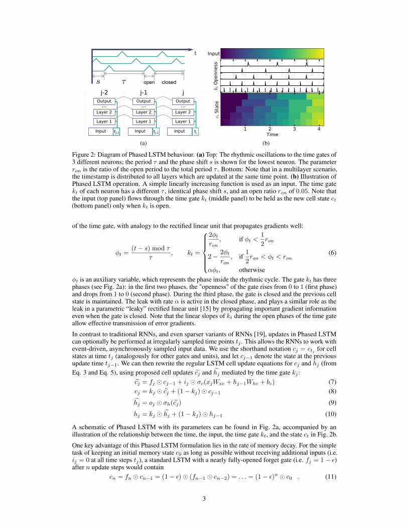
Figure 3: Frequency discrimination task. The network is trained to discriminate waves of differentfrequency sets (shown in blue and gray); every circle is an input point. (a) Standard condition: thedata is regularly sampled every 1 ms. (b) High resolution sampling condition: new input pointsare gathered every 0.1ms. (c) Asynchronous sampling condition: new input points are presented atintervals of 0.02 ms to 10 ms. (d) The accuracy of Phased LSTM under the three sampling conditionsis maintained, but the accuracy of the BN-LSTM and standard LSTM drops significantly in thesampling conditions (b) and (c). Error bars indicate standard deviation over 5 runs.

This means the memory for ε < 1 decays exponentially with every time step. Conversely, the PhasedLSTM state only decays during the open periods of the time gate, but maintains a perfect memoryduring its closed phase, i.e. cj = cj−∆ if kt = 0 for tj−∆ ≤ t ≤ tj . Thus, during a single oscillationperiod of length τ , the units only update during a duration of ron · τ , which will result in substantiallyfewer than n update steps. Because of this cyclic memory, Phased LSTM can have much longer andadjustable memory length via the parameter τ .

The oscillations impose sparse updates of the units, therefore substantially decreasing the total numberof updates during network operation. During training, this sparseness ensures that the gradient isrequired to backpropagate through fewer updating timesteps, allowing an undecayed gradient to bebackpropagated through time and allowing faster learning convergence. Similar to the shielding ofthe cell state ct (and its gradient) by the input gates and forget gates of the LSTM, the time gateprevents external inputs and time steps from dispersing and mixing the gradient of the cell state.

3 Results

In the following sections, we investigate the advantages of the Phased LSTM model in a varietyof scenarios that require either precise timing of updates or learning from a long sequence. For allthe results presented here, the networks were trained with Adam [18] set to default learning rateparameters, using Theano [2] with Lasagne [9]. Unless otherwise specified, the leak rate was set toα = 0.001 during training and α = 0 during test. The phase shift, s, for each neuron was uniformlychosen from the interval [0, τ ]. The parameters τ and s were learned during training, while the openratio ron was fixed at 0.05 and not adjusted during training, except in the first task to demonstratethat the model can train successfully while learning all parameters.

3.1 Frequency Discrimination Task

In this first experiment, the network is trained to distinguish two classes of sine waves from differentfrequency sets: those with a period in a target range T ∼ U(5, 6), and those outside the range, i.e.T ∼ {U(1, 5) ∪ U(6, 100)}, using U(a, b) for the uniform distribution on the interval (a, b). Thistask illustrates the advantages of Phased LSTM, since it involves a periodic stimulus and requiresfine timing discrimination. The inputs are presented as pairs 〈y, t〉, where y is the amplitude and tthe timestamp of the sample from the input sine wave.

Figure 3 illustrates the task: the blue curves must be separated from the lighter curves based onthe samples shown as circles. We evaluate three conditions for sampling the input signals: In thestandard condition (Fig. 3a), the sine waves are regularly sampled every 1 ms; in the oversampled

4

0 50 100 150 200 250 300Epoch

45

50

55

60

65

70

75

80

85

90

Acc

ura

cy [

%] Phased LSTM

BN LSTMLSTM

(a)

0 20 40 60 80 100Epoch

10-5

10-4

10-3

10-2

10-1

100

MSE

LSTMPLSTM (¿» eU(0; 2))PLSTM (¿» eU(2; 4))PLSTM (¿» eU(4; 6))PLSTM (¿» eU(6; 8))

(b)

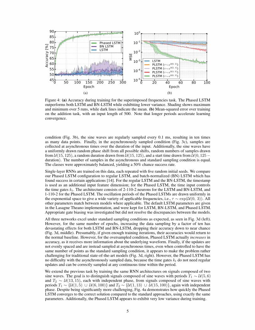
Figure 4: (a) Accuracy during training for the superimposed frequencies task. The Phased LSTMoutperforms both LSTM and BN-LSTM while exhibiting lower variance. Shading shows maximumand minimum over 5 runs, while dark lines indicate the mean. (b) Mean-squared error over trainingon the addition task, with an input length of 500. Note that longer periods accelerate learningconvergence.

condition (Fig. 3b), the sine waves are regularly sampled every 0.1 ms, resulting in ten timesas many data points. Finally, in the asynchronously sampled condition (Fig. 3c), samples arecollected at asynchronous times over the duration of the input. Additionally, the sine waves havea uniformly drawn random phase shift from all possible shifts, random numbers of samples drawnfrom U(15, 125), a random duration drawn from U(15, 125), and a start time drawn from U(0, 125−duration). The number of samples in the asynchronous and standard sampling condition is equal.The classes were approximately balanced, yielding a 50% chance success rate.

Single-layer RNNs are trained on this data, each repeated with five random initial seeds. We compareour Phased LSTM configuration to regular LSTM, and batch-normalized (BN) LSTM which hasfound success in certain applications [14]. For the regular LSTM and the BN-LSTM, the timestampis used as an additional input feature dimension; for the Phased LSTM, the time input controlsthe time gates kt. The architecture consists of 2-110-2 neurons for the LSTM and BN-LSTM, and1-110-2 for the Phased LSTM. The oscillation periods of the Phased LSTMs are drawn uniformly inthe exponential space to give a wide variety of applicable frequencies, i.e., τ ∼ exp(U(0, 3)). Allother parameters match between models where applicable. The default LSTM parameters are givenin the Lasagne Theano implementation, and were kept for LSTM, BN-LSTM, and Phased LSTM.Appropriate gate biasing was investigated but did not resolve the discrepancies between the models.

All three networks excel under standard sampling conditions as expected, as seen in Fig. 3d (left).However, for the same number of epochs, increasing the data sampling by a factor of ten hasdevastating effects for both LSTM and BN-LSTM, dropping their accuracy down to near chance(Fig. 3d, middle). Presumably, if given enough training iterations, their accuracies would return tothe normal baseline. However, for the oversampled condition, Phased LSTM actually increases inaccuracy, as it receives more information about the underlying waveform. Finally, if the updates arenot evenly spaced and are instead sampled at asynchronous times, even when controlled to have thesame number of points as the standard sampling condition, it appears to make the problem ratherchallenging for traditional state-of-the-art models (Fig. 3d, right). However, the Phased LSTM hasno difficulty with the asynchronously sampled data, because the time gates kt do not need regularupdates and can be correctly sampled at any continuous time within the period.

We extend the previous task by training the same RNN architectures on signals composed of twosine waves. The goal is to distinguish signals composed of sine waves with periods T1 ∼ U(5, 6)and T2 ∼ U(13, 15), each with independent phase, from signals composed of sine waves withperiods T1 ∼ {U(1, 5) ∪ U(6, 100)} and T2 ∼ {U(1, 13) ∪ U(15, 100)}, again with independentphase. Despite being significantly more challenging, Fig. 4a demonstrates how quickly the PhasedLSTM converges to the correct solution compared to the standard approaches, using exactly the sameparameters. Additionally, the Phased LSTM appears to exhibit very low variance during training.

5

12

3

(a) (b)

0

1×10

5

Time [us]

2

3

(c)

Figure 5: N-MNIST experiment. (a) Sketch of digit movement seen by the image sensor. (b)Frame-based representation of an ‘8’ digit from the N-MNIST dataset [24] obtained by integrating allinput spikes for each pixel. (c) Spatio-temporal representation of the digit, presented in three saccadesas in (a). Note that this representation shows the digit more clearly than the blurred frame-based one.

3.2 Adding Task

To investigate how introducing time gates helps learning when long memory is required, we revisitan original LSTM task called the adding task [16]. In this task, a sequence of random numbersis presented along with an indicator input stream. When there is a 0 in the indicator input stream,the presented value should be ignored; a 1 indicates that the value should be added. At the end ofpresentation the network produces a sum of all indicated values. Unlike the previous tasks, there is noinherent periodicity in the input, and it is one of the original tasks that LSTM was designed to solvewell. This would seem to work against the advantages of Phased LSTM, but using a longer period forthe time gate kt could allow more effective training as a unit opens only a for a few timesteps duringtraining.

In this task, a sequence of numbers (of length 490 to 510) was drawn from U(−0.5, 0.5). Twonumbers in this stream of numbers are marked for addition: one from the first 10% of numbers(drawn with uniform probability) and one in the last half (drawn with uniform probability), producinga model of a long and noisy stream of data with only few significant points. Importantly, this shouldchallenge the Phased LSTM model because there is no inherent periodicity and every timestep couldcontain the important marked points.

The same network architecture is used as before. The period τ was drawn uniformly in the expo-nential domain, comparing four sampling intervals exp(U(0, 2)), exp(U(2, 4)), exp(U(4, 6)), andexp(U(6, 8)). Note that despite different τ values, the total number of LSTM updates remains ap-proximately the same, since the overall sparseness is set by ron. However, a longer period τ providesa longer jump through the past timesteps for the gradient during backpropagation-through-time.

Moreover, we investigate whether the model can learn longer sequences more effectively when longerperiods are used. By varying the period τ , the results in Fig. 4b show longer τ accelerates training ofthe network to learn much longer sequences faster.

3.3 N-MNIST Event-Based Visual Recognition

To test performance on real-world asynchronously sampled data, we make use of the publicly-available N-MNIST [24] dataset for neuromorphic vision. The recordings come from an event-basedvision sensor that is sensitive to local temporal contrast changes [26]. An event is generated froma pixel when its local contrast change exceeds a threshold. Every event is encoded as a 4-tuple〈x, y, p, t〉 with position x, y of the pixel, a polarity bit p (indicating a contrast increase or decrease),and a timestamp t indicating the time when the event is generated. The recordings consist of eventsgenerated by the vision sensor while the sensor undergoes three saccadic movements facing a staticdigit from the MNIST dataset (Fig. 5a). An example of the event responses can be seen in Fig. 5c).

In previous work using event-based input data [21, 23], the timing information was sometimesremoved and instead a frame-based representation was generated by computing the pixel-wiseevent-rate over some time period (as shown in Fig. 5(b)). Note that the spatio-temporal surface of

6

Table 1: Accuracy on N-MNISTCNN BN-LSTM Phased LSTM (τ = 100ms)

Accuracy at Epoch 1 73.81% ± 3.5 40.87% ± 13.3 90.32% ± 2.3Train/test ρ = 0.75 95.02% ± 0.3 96.93% ± 0.12 97.28% ± 0.1Test with ρ = 0.4 90.67% ± 0.3 94.79% ± 0.03 95.11% ± 0.2Test with ρ = 1.0 94.99% ± 0.3 96.55% ± 0.63 97.27% ± 0.1LSTM Updates – 3153 per neuron 159 ± 2.8 per neuron

events in Fig. 5(c) reveals details of the digit much more clearly than in the blurred frame-basedrepresentation.The Phased LSTM allows us to operate directly on such spatio-temporal event streams.

Table 1 summarizes classification results for three different network types: a CNN trained on frame-based representations of N-MNIST digits and two RNNs, a BN-LSTM and a Phased LSTM, traineddirectly on the event streams. Regular LSTM is not shown, as it was found to perform worse. TheCNN was comprised of three alternating layers of 8 kernels of 5x5 convolution with a leaky ReLUnonlinearity and 2x2 max-pooling, which were then fully-connected to 256 neurons, and finally fully-connected to the 10 output classes. The event pixel address was used to produce a 40-dimensionalembedding via a learned embedding matrix [9], and combined with the polarity to produce the input.Therefore, the network architecture was 41-110-10 for the Phased LSTM and 42-110-10 for theBN-LSTM, with the time given as an extra input dimension to the BN-LSTM.

Table 1 shows that Phased LSTM trains faster than alternative models and achieves much higheraccuracy with a lower variance even within the first epoch of training. We further define a factor, ρ,which represents the probability that an event is included, i.e. ρ = 1.0 means all events are included.The RNN models are trained with ρ = 0.75, and again the Phased LSTM achieves slightly higherperformance than the BN-LSTM model. When testing with ρ = 0.4 (fewer events) and ρ = 1.0 (moreevents) without retraining, both RNN models perform well and greatly outperform the CNN. This isbecause the accumulated statistics of the frame-based input to the CNN change drastically when theoverall spike rates are altered. The Phased LSTM RNNs seem to have learned a stable spatio-temporalsurface on the input and are only slightly altered by sampling it more or less frequently.

Finally, as each neuron of the Phased LSTM only updates about 5% of the time, on average, 159updates are needed in comparison to the 3153 updates needed per neuron of the BN-LSTM, leadingto an approximate twenty-fold reduction in run time compute cost. It is also worth noting that theseresults form a new state-of-the-art accuracy for this dataset [24, 7].

3.4 Visual-Auditory Sensor Fusion for Lip Reading

Finally, we demonstrate the use of Phased LSTM on a task involving sensors with different samplingrates. Few RNN models ever attempt to merge sensors of different input frequencies, although thesampling rates can vary substantially. For this task, we use the GRID dataset [8]. This corpus containsvideo and audio of 30 speakers each uttering 1000 sentences composed of a fixed grammar and aconstrained vocabulary of 51 words. The data was randomly divided into a 90%/10% train-test set.An OpenCV [17] implementation of a face detector was used on the video stream to extract the facewhich was then resized to grayscale 48x48 pixels. The goal here is to obtain a model that can useaudio alone, video alone, or both inputs to robustly classify the sentence. However, since the audioalone is sufficient to achieve greater than 99% accuracy, sensor modalities were randomly masked tozero during training to encourage robustness towards sensory noise and loss.

The network architecture first separately processes video and audio data before merging them intwo RNN layers that receive both modalities. The video stream uses three alternating layers of 16kernels of 5x5 convolution and 2x2 subsampling to reduce the input of 1x48x48 to 16x2x2, which isthen used as the input to 110 recurrent units. The audio stream connects the 39-dimensional MFCCs(13 MFCCs with first and second derivatives) to 150 recurrent units. Both streams converge intothe Merged-1 layer with 250 recurrent units, and is connected to a second hidden layer with 250recurrent units named Merged-2. The output of the Merged-2 layer is fully-connected to 51 outputnodes, which represent the vocabulary of GRID. For the Phased LSTM network, all recurrent unitsare Phased LSTM units.

7

Time

MFCCs

Inputs

VideoFrames

220 260 300 340Time [ms]

Merged-2PLSTM

Merged-1PLSTM

VideoPLSTM

AudioPLSTM

kj O

penness

(a)

500 1500 2500Time [ms]

05

101520253035

MFC

C

(b)

10-2

10-1

Low

Res.

Loss

0 10 20 30 40 50Epoch

10-2

10-1

Hig

h R

es.

Loss

Phased LSTMBN LSTMLSTM

(c)

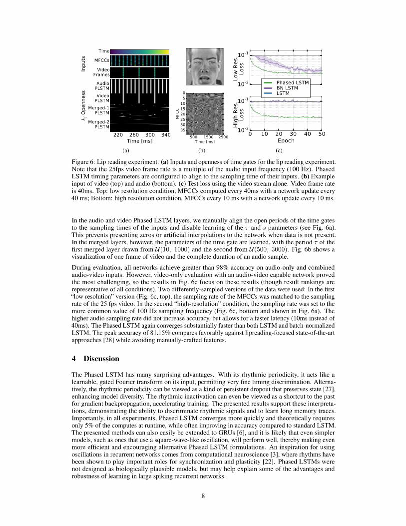
Figure 6: Lip reading experiment. (a) Inputs and openness of time gates for the lip reading experiment.Note that the 25fps video frame rate is a multiple of the audio input frequency (100 Hz). PhasedLSTM timing parameters are configured to align to the sampling time of their inputs. (b) Exampleinput of video (top) and audio (bottom). (c) Test loss using the video stream alone. Video frame rateis 40ms. Top: low resolution condition, MFCCs computed every 40ms with a network update every40 ms; Bottom: high resolution condition, MFCCs every 10 ms with a network update every 10 ms.

In the audio and video Phased LSTM layers, we manually align the open periods of the time gatesto the sampling times of the inputs and disable learning of the τ and s parameters (see Fig. 6a).This prevents presenting zeros or artificial interpolations to the network when data is not present.In the merged layers, however, the parameters of the time gate are learned, with the period τ of thefirst merged layer drawn from U(10, 1000) and the second from U(500, 3000). Fig. 6b shows avisualization of one frame of video and the complete duration of an audio sample.

During evaluation, all networks achieve greater than 98% accuracy on audio-only and combinedaudio-video inputs. However, video-only evaluation with an audio-video capable network provedthe most challenging, so the results in Fig. 6c focus on these results (though result rankings arerepresentative of all conditions). Two differently-sampled versions of the data were used: In the first“low resolution” version (Fig. 6c, top), the sampling rate of the MFCCs was matched to the samplingrate of the 25 fps video. In the second “high-resolution” condition, the sampling rate was set to themore common value of 100 Hz sampling frequency (Fig. 6c, bottom and shown in Fig. 6a). Thehigher audio sampling rate did not increase accuracy, but allows for a faster latency (10ms instead of40ms). The Phased LSTM again converges substantially faster than both LSTM and batch-normalizedLSTM. The peak accuracy of 81.15% compares favorably against lipreading-focused state-of-the-artapproaches [28] while avoiding manually-crafted features.

4 Discussion

The Phased LSTM has many surprising advantages. With its rhythmic periodicity, it acts like alearnable, gated Fourier transform on its input, permitting very fine timing discrimination. Alterna-tively, the rhythmic periodicity can be viewed as a kind of persistent dropout that preserves state [27],enhancing model diversity. The rhythmic inactivation can even be viewed as a shortcut to the pastfor gradient backpropagation, accelerating training. The presented results support these interpreta-tions, demonstrating the ability to discriminate rhythmic signals and to learn long memory traces.Importantly, in all experiments, Phased LSTM converges more quickly and theoretically requiresonly 5% of the computes at runtime, while often improving in accuracy compared to standard LSTM.The presented methods can also easily be extended to GRUs [6], and it is likely that even simplermodels, such as ones that use a square-wave-like oscillation, will perform well, thereby making evenmore efficient and encouraging alternative Phased LSTM formulations. An inspiration for usingoscillations in recurrent networks comes from computational neuroscience [3], where rhythms havebeen shown to play important roles for synchronization and plasticity [22]. Phased LSTMs werenot designed as biologically plausible models, but may help explain some of the advantages androbustness of learning in large spiking recurrent networks.

8

References[1] D. Bahdanau, K. Cho, and Y. Bengio. Neural machine translation by jointly learning to align and translate.

arXiv preprint arXiv:1409.0473, 2014.[2] J. Bergstra, O. Breuleux, F. Bastien, P. Lamblin, R. Pascanu, G. Desjardins, J. Turian, D. Warde-Farley,

and Y. Bengio. Theano: a CPU and GPU math expression compiler. In Proceedings of the Python forscientific computing conference (SciPy), volume 4, page 3, 2010.

[3] G. Buzsaki. Rhythms of the Brain. Oxford University Press, 2006.[4] G. Cauwenberghs. An analog VLSI recurrent neural network learning a continuous-time trajectory. IEEE

Transactions on Neural Networks, 7(2):346–361, 1996.[5] K. Cho, A. Courville, and Y. Bengio. Describing multimedia content using attention-based encoder-decoder

networks. IEEE Transactions on Multimedia, 17(11):1875–1886, 2015.[6] K. Cho, B. van Merrienboer, C. Gulcehre, F. Bougares, H. Schwenk, and Y. Bengio. Learning phrase repre-

sentations using RNN encoder-decoder for statistical machine translation. arXiv preprint arXiv:1406.1078,2014.

[7] G. K. Cohen, G. Orchard, S. H. Ieng, J. Tapson, R. B. Benosman, and A. van Schaik. Skimming digits:Neuromorphic classification of spike-encoded images. Frontiers in Neuroscience, 10(184), 2016.

[8] M. Cooke, J. Barker, S. Cunningham, and X. Shao. An audio-visual corpus for speech perception andautomatic speech recognition. The Journal of the Acoustical Society of America, 120(5):2421–2424, 2006.

[9] S. Dieleman et al. Lasagne: First release., Aug. 2015.[10] K.-I. Funahashi and Y. Nakamura. Approximation of dynamical systems by continuous time recurrent

neural networks. Neural Networks, 6(6):801–806, 1993.[11] F. A. Gers and J. Schmidhuber. Recurrent nets that time and count. In Neural Networks, 2000. IJCNN

2000, Proceedings of the IEEE-INNS-ENNS International Joint Conference on, volume 3, pages 189–194.IEEE, 2000.

[12] A. Graves. Generating sequences with recurrent neural networks. arXiv preprint arXiv:1308.0850, 2013.[13] A. Graves, A.-R. Mohamed, and G. Hinton. Speech recognition with deep recurrent neural networks.

In 2013 IEEE International Conference on Acoustics, Speech and Signal Processing (ICASSP), pages6645–6649, 2013.

[14] A. Hannun, C. Case, J. Casper, B. Catanzaro, G. Diamos, E. Elsen, R. Prenger, S. Satheesh, S. Sengupta,A. Coates, et al. Deep speech: Scaling up end-to-end speech recognition. arXiv preprint arXiv:1412.5567,2014.

[15] K. He, X. Zhang, S. Ren, and J. Sun. Delving deep into rectifiers: Surpassing human-level performance onimagenet classification. In The IEEE International Conference on Computer Vision (ICCV), 2015.

[16] S. Hochreiter and J. Schmidhuber. Long short-term memory. Neural Computation, 9(8):1735–1780, 1997.[17] Itseez. Open source computer vision library. https://github.com/itseez/opencv, 2015.[18] D. Kingma and J. Ba. Adam: A method for stochastic optimization. arXiv preprint arXiv:1412.6980, 2014.[19] J. Koutnik, K. Greff, F. Gomez, and J. Schmidhuber. A clockwork rnn. arXiv preprint arXiv:1402.3511,

2014.[20] T. Mikolov, M. Karafiát, L. Burget, J. Cernocky, and S. Khudanpur. Recurrent neural network based

language model. Interspeech, 2:3, 2010.[21] D. Neil and S.-C. Liu. Effective sensor fusion with event-based sensors and deep network architectures. In

IEEE Int. Symposium on Circuits and Systems (ISCAS), 2016.[22] B. Nessler, M. Pfeiffer, L. Buesing, and W. Maass. Bayesian computation emerges in generic cortical

microcircuits through spike-timing-dependent plasticity. PLoS Comput Biol, 9(4):e1003037, 2013.[23] P. O’Connor, D. Neil, S.-C. Liu, T. Delbruck, and M. Pfeiffer. Real-time classification and sensor fusion

with a spiking Deep Belief Network. Frontiers in Neuroscience, 7, 2013.[24] G. Orchard, A. Jayawant, G. Cohen, and N. Thakor. Converting static image datasets to spiking neuromor-

phic datasets using saccades. arXiv: 1507.07629, 2015.[25] B. A. Pearlmutter. Learning state space trajectories in recurrent neural networks. Neural Computation,

1(2):263–269, 1989.[26] C. Posch, T. Serrano-Gotarredona, B. Linares-Barranco, and T. Delbruck. Retinomorphic event-based

vision sensors: bioinspired cameras with spiking outputs. Proceedings of the IEEE, 102(10):1470–1484,2014.

[27] S. Semeniuta, A. Severyn, and E. Barth. Recurrent dropout without memory loss. arXiv, arXiv:1603.05118,2016.

[28] M. Wand, J. Koutník, and J. Schmidhuber. Lipreading with long short-term memory. arXiv preprintarXiv:1601.08188, 2016.

[29] K. Xu, J. Ba, R. Kiros, K. Cho, A. Courville, R. Salakhutdinov, R. Zemel, and Y. Bengio. Show, attendand tell: Neural image caption generation with visual attention. In International Conference on MachineLearning, 2015.

9