Phase unwrapping algorithms for radar interferometry...

586 J. Opt. Soc. Am. A/Vol. 15, No. 3 /March 1998 H. A. Zebker and Y. Lu

Phase unwrapping algorithms for radarinterferometry: residue-cut,

least-squares, and synthesis algorithms

Howard A. Zebker and Yanping Lu

Department of Geophysics, Stanford University, Stanford, California 94305-2215

Received May 5, 1997; accepted September 18, 1997; revised manuscript received October 9, 1997

The advent of interferometric synthetic aperature radar for geophysical studies has resulted in the need foraccurate, efficient methods of two-dimensional phase unwrapping. Inference of the lost integral number ofcycles in phase measurements is critical for three-pass surface deformation studies as well as topographic map-ping and can result in an order of magnitude increase in sensitivity for two-pass deformation analysis. Whilephase unwrapping algorithms have proliferated over the past ten years, two main approaches are currently inuse. Each is most useful only for certain restricted applications. All these algorithms begin with the mea-sured gradient of the phase field, which is subsequently integrated to recover the unwrapped phases. Theearliest approaches in interferometric applications incorporated residue identification and cuts to limit thepossible integration paths, while a second class using least-squares techniques was developed in the early1990’s. We compare the approaches and find that the residue-cut algorithms are quite accurate but do notproduce estimates in regions of moderate phase noise. The least-squares methods yield complete coverage butat the cost of distortion in the recovered phase field. A new synthesis approach, combining the cuts from thefirst class with a least-squares solution, offers greater spatial coverage with less distortion in many instances.© 1998 Optical Society of America [S0740-3232(98)01403-3]

OCIS codes: 280.0180, 280.6730, 120.3180.

1. INTRODUCTIONAlgorithms that relate individual phase measurementson a two-dimensional field, motivated largely by interestin interferometric synthetic aperture radar (SAR) tech-niques, have proliferated over the past ten years.1–4

These algorithms seek to infer the integral number ofcycles lost when a phase measurement is made from atwo-dimensional complex signal amplitude observation,which uniquely identifies only the phase value modulo 2p.We refer to such algorithms here as phase unwrapping, asdistinguished from the use of that term for reconstructionof signal amplitudes from frequency-domain phase data, acommon problem associated with one-dimensional signalprocessing.

We report here a comparison of several of the phase un-wrapping algorithms in more common use today andidentify and contrast the strengths and weaknesses ofeach. We also present a synthesis approach that com-bines some of the more effective features of the existingalgorithms and can extend the range of phase unwrap-ping situations amenable to automated solution. Ratherthan revolutionize present capabilities, these new algo-rithms represent another approach for phase unwrappingprocedures that aid in some situations where the existingalgorithms fare poorly. Because we (1) do not revieweach existing algorithm comprehensively, (2) do proposenew variations of the algorithms suited to particularstyles of input data, and (3) do not believe that the exist-ing set of approaches is the final word on phase unwrap-ping procedures, this article serves more as a progress re-

0740-3232/98/030586-13$10.00 ©

port rather than as a review of phase unwrappingprocedures.

The advent of interferometric SAR for geophysicalstudies, in particular, has resulted in the need for accu-rate, efficient methods of two-dimensional phase unwrap-ping. Radar methods for fast and precise measurementof topographic data,5,6 determination of centimeter-levelsurface deformation fields,7–9 and surface velocityfields10,11 all require that the relative phases over largeareas be known. Strictly speaking, each of these tech-niques requires, in addition, knowledge of the absolutephase values;12 however, in practice contextual clues orknown fiducial values (tie points) often permit geophysi-cal inference with only the relative phases, given that thephase field is unwrapped.

Although many insights into underlying surface pro-cesses may be obtained by visual inspection of the initial,wrapped radar interferogram,13,14 this unwrapping by eyemay be applied only to simple phase fields without signifi-cant and complicated structure. Moreover, automatedtopographic mapping approaches and the application ofthree-pass deformation algorithms are precluded by thenecessity of human interaction on a pixel-by-pixel levelwith the interferometric data. For instance, even asmall-area topographic map may contain millions ofmeter-spaced posts. Accuracy also drives the require-ment. In regions of finely spaced fringes, it may be diffi-cult to estimate the phase manually to better than a largefraction of a cycle accuracy, whereas performance of theradar system itself allows accuracies corresponding to

1998 Optical Society of America

H. A. Zebker and Y. Lu Vol. 15, No. 3 /March 1998/J. Opt. Soc. Am. A 587

perhaps 3 deg of phase.12,15 Requirements for futureradar system performance typically imply that theinterferogram phase can be determined to similar if notbetter levels.

All of the commonly used phase unwrapping algo-rithms relate the phase values by first differentiating thephase field and subsequently reintegrating, adding backthe missing integral cycles to obtain a more continuousresult. The many algorithms proposed for phase un-wrapping over the past few years fall into two basicclasses: (1) algorithms based on identification of resi-dues in the wrapped phase field and cuts, or ‘‘trees,’’ con-necting a group of residues to limit the integration paths,and (2) algorithms that derive a smooth field by integrat-ing the gradient of the observations subject to smoothnessconstraints as determined by least-squared-difference cri-teria. Least-squares algorithms may be weighted or un-weighted; that is, they may consider the closeness of fit asdependent on ancillary data for each measurement pointsuch as the radar brightness or correlation, giving greaterweight to those points deemed to be more accurate. Notethat weighted least-squares solutions need not be smoothor even continuous, if zero weights are assigned to somepoints in the phase data. This property will form the ba-sis of our proposed improvement on the traditionalweighted least-squares solution, consisting essentially ofa method to assign the zero weights that is dependent onphase observables.

Another solution, derived from a mathematical theoryutilizing a Green’s-function reconstruction,4 has recentlybeen shown to be equivalent to the least-squares solution,differing only in terms of computational efficiency.16

Other approaches in today’s literature use nested combi-nations of least-squares techniques17 and methods em-ploying measures of data integrity to guide unwrappingpaths,18 as well as several employing neural network or‘‘genetic’’ algorithms.19 However, these latter ap-proaches have not gained widespread acceptance and wewill not analyze them here. They may be useful, or evenoutperform the more common algorithms, for specializedsituations.

This paper is constructed as follows. First, we brieflyillustrate and summarize the phase unwrapping problemand describe the solution approaches of the two principalalgorithm classes. We also introduce a synthesis algo-rithm that combines features of both classes in a singlealgorithm. Next, we illustrate the performance of eachalgorithm in a variety of situations that differ in the char-acter of the phase field to be unwrapped. We conclude bystating that phase unwrapping remains a significant is-sue in interferometric SAR analysis and that the synthe-sis approach presented here contributes one more tech-nique that is to be added to the collection of algorithmsavailable for any given application.

2. PHASE UNWRAPPING: THE PROBLEMAND TWO SOLUTION APPROACHESIn interferometric SAR analysis, two radar images of thesame surface area are acquired and differenced in phase,forming a radar interferogram. This is usually imple-

mented by cross multiplying the complex reflectivity ateach point of one image by its corresponding conjugatevalue in the second image, so that the interferogram alsopreserves useful information about the signal amplitudes.

The complex signal amplitude reflected from each ra-dar resolution element in a single image consists of thevector sum of contributions from many individual scatter-ing elements within that resolution element. Becausethe size of the resolution element is typically many wave-lengths, randomness in the spatial distribution of thescatterers yields an approximately uniform phase distri-bution in the resultant coherent sum of the scatteredwaves. The phases, however random, are nonethelessdeterministic in that they are calculable from knowledgeof the precise locations of each scattering center. If thepair of images forming the radar interferogram are dupli-cates precisely regarding viewing geometry and antennapolarization, if receiver noise effects are minimal, and ifthe surface itself is unchanged between observations, thetwo images will be identical and the interferogram willexhibit zero phase everywhere.

On the other hand, if the viewing geometry is alteredwithin certain limits, the phase differences comprisingthe interferogram will vary across the terrain in a man-ner related to the surface topography.5,20 In addition, ifthe viewing geometry is unchanged but one region of thesurface itself is displaced spatially with respect to the restof the image, the pixels corresponding to that section willexhibit phase differences proportional to the line-of-sightcomponent of the displacement.7 Finally, if displace-ments are not coherent across each resolution elementbut instead randomize the positions of each scatterer withrespect to others inside the element, the pair of echoeswill be less well related and the coherence, or correlation,of the interferogram will decrease,21 resulting in a noisethat may mask the underlying phase signature.

The interferometric phase signatures vary relativelysmoothly from point to point in the interferogram andmay be inverted to recover surface topography, velocity,or displacement fields. However, the phase observablesare measured modulo 2p; that is, the integral number ofphase cycles on each measurement is lost. Consequently,if the surface displacement in a scene is greater than one-half radar wavelength and the resulting interferogramphase excursion is greater than one cycle, or if the combi-nation of interferometric baseline and surface topographyyields more than one fringe of topographic signature, theinterferogram cannot be uniquely inverted without a pro-cedure to recover the missing cycles. We refer to suchprocedures as phase unwrapping.

Phase unwrapping algorithms share a common initialapproach: the phase change, or gradient, from one pointto the next in an interferogram is computed and then in-tegrated to form a single, smoother phase function incor-porating the previously missing cycles. To date all algo-rithms applied to interferometric SAR have usedvariations of measured phase gradient integration proce-dures.

The first constraint on a phase unwrapping algorithmis that it produce consistent results; that is, the samephase field should be recovered independently of the di-rection and order chosen for the phase difference integra-


tion. The problem can be illustrated by the following setof measurements, corresponding to a four-by-four pixel in-terferogram array, each expressed in cycles:

0.2 0.0 0.8 0.00.4 0.2 0.2 0.40.6 0.8 0.8 0.60.8 0.8 0.8 0.8

We assume that the data are adequately sampled; to sat-isfy Nyquist we cannot have a jump of more than one-halfcycle from point to point. To unwrap these data, we canintegrate the top line across from left to right, adding in-tegral cycles to ensure that the jump from one point to thenext in all directions is less one-half cycle, and then inte-grate down each column. The result of this procedure is

0.2 0.0 20.2 0.00.4 0.2 0.2 0.40.6 20.2 20.2 0.60.8 20.2 20.2 0.8

Now, transpose the directions of integration. First un-wrap down the leftmost column and then across each row:

0.2 0.0 20.2 0.00.4 0.2 0.2 0.40.6 0.8 0.8 0.60.8 0.8 0.8 0.8

These results are different, and only one of these solu-tions at most can be correct. They differ in that four ofthe measurements are one cycle greater in the second in-stance than in the first. This inconsistency must beeliminated in any practical algorithm.

A little reflection leads to the conclusion that for a con-sistent result, any closed line integral in the phase fieldmust equal zero; that is, the phase along the path mustreturn to its starting value. Using this approach, the in-consistency in the above example can be traced to the ex-istence of residues in the measured phase field, regionsthat are self-inconsistent. Consider a short circularphase path extracted from the above example:

0.4 0.20.6 0.8

Integrating clockwise around the loop yields a net 21cycle instead of the zero sum required by consistency.We thus term this set of four phase measurements anegative phase residue, drawing on a mathematical anal-ogy with Cauchy integration in the complex plane. Infact any closed path on the phase field containing thisresidue will yield the same net 21 cycle unless the pathcontains additional residues. If the net charge withinthe integration paths is zero, the result will be consistent.Therefore it is the goal of the phase unwrapping proce-dure to eliminate potential integration paths enclosingunequal numbers of positive and negative residues. Theresidue-cut algorithms do this explicitly, whereas theleast-squares procedures described to date exhibit arti-

facts generated by the existence of the residues. Thesynthesis approach proposed here incorporates residueavoidance with the least-squares solution.

Residues derive from two sources in the radarmeasurements.1 The first is actual discontinuities in thedata. The fringe spacing may be so fine on certain topo-graphic slopes or from large interobservation displace-ment as to exceed the Nyquist criterion of half-cycle spac-ing. The second is noise in the data set, whether fromthermal and other noise sources or from decorrelation dueto baseline length and temporal change in the scene.20–22

Residues from whatever source require compensation inthe phase unwrapping procedure.

A. Residue-Cut Tree AlgorithmsThe initial residue-cut phase unwrapping procedure pro-posed by Goldstein et al.1 is implemented by first identi-fying the locations of all residues in an interferogram andthen connecting the residues with branch cuts to preventthe existence of integration paths that can encircle unbal-anced numbers of positive and negative residues. Be-cause of the terminology of branch cuts and the dendriticappearance of the complete set of cuts, the interconnec-tion of the residues was referred to as growing ‘‘trees’’ bythe authors.

The residue-cut algorithm of Goldstein et al., in com-mon use today, is a relatively conservative algorithm inthat it tends to grow rather dense networks of trees inresidue-rich regions. The algorithm initially connectsclosely spaced, oppositely charged, pairs of residues withcuts that prevent integration paths between them, help-ing to ensure consistency. If all permitted integrationpaths enclose equal numbers of positive and negativeresidues—that is, each tree connects the same number ofplus and minus charges and is in that sense uncharged—consistency is assured. Progressively longer trees arepermitted until all residues are connected to at least oneother residue and until the net charge on each tree iszero. Networks of small trees are used to prevent anysingle branch from becoming too long and isolating largesubareas from the rest of the image.

Specifically, the tree-growth algorithm of Goldsteinet al.1 consists of the following steps:

1. Residues are identified and marked as either posi-tive or negative.

2. The interferogram phase field is scanned system-atically until a residue is located.

3. From that residue, the surrounding area issearched until another residue is found. A cut is formedbetween the residues and the total charge is computed.

4. If the total charge along the tree is zero, the tree isconsidered complete and the systematic scan of step (2) iscontinued.

5. If the total charge is nonzero, the search continuesfor nearby residues. As each residue is encountered, it isconnected to the tree by means of a branch cut and thetotal charge is computed. Only when the total charge iszero is the tree considered complete and the step (2) scanallowed to proceed.

In the course of the search for residues, all residues, re-gardless of whether each has been previously assigned to


a tree, are added to the new tree. This yields the den-dritic appearance of the cuts and the nomenclature‘‘trees.’’

Finally, when a boundary of the scene is encountered, acut is drawn to the boundary and the tree is deemed com-plete and uncharged. This superconducting property ofthe edges prevents overly long trees from isolating largeareas of the image.

A consequence of the indiscriminate branch growth un-til charge neutrality is achieved for all trees, and all resi-dues are accounted for, is that in residue-rich regions,such as heavily laid over or very noisy regions, the treegrowth is so dense that the region is isolated from the re-mainder of the image and no unwrapped phase estimatecan be obtained. This conservative approach nearlyeliminates mistakes at the expense of providing an incom-plete unwrapping result.

An unpublished variant of this algorithm was devel-oped by Atsushi Hiramatsu at Caltech in the early 1990’s;nevertheless, the algorithm and code survive among thephase unwrapping underground. In the Atsushi ap-proach, residues are determined as before, but the treesare prevented from closing on themselves and thus a so-lution is forced at every point in the image. This solu-tion, although consistent and complete, is not alwayscorrect—the algorithm typically generates regional errorsin the noisy and laid over portions of the interferogramimage. In many situations the gain from complete un-wrapping solutions outweighs the cost of the errors, butthis must be determined on a case-by-case basis.

Another version of the residue-cut algorithm again be-gins with the method of Goldstein et al.1 but allows opera-tor interaction to edit the trees manually before phase in-tegration, thus permitting more integration paths thanthe conservative initial algorithm allows. In this mannerintegration paths may be opened up into areas that weretoo densely packed with residues to unwrap. Here againthe trade-off is for increased areal coverage at the ex-pense of possible errors, but the additional coverage anderrors may be precisely controlled by the skill of the op-erator in identifying appropriate trees to prune. How-ever, it transforms the procedure from a fully automatedone to one requiring intense operator interaction on eachinterferogram. For limited applications this may be ac-ceptable. (This editing approach was used by Zebkeret al.9 to maximize the unwrapped area in the analysis ofsurface deformation resulting from the Landers 1992earthquake.)

B. Least-Squares AlgorithmsThe second major approach to phase unwrapping in com-mon use today was presented by Ghiglia and Romero,2

who applied a mathematical formalism first developed byHunt23 to the radar interferometry phase unwrappingproblem. Hunt developed a matrix formulation suitablefor general phase reconstruction problems; Ghiglia andRomero found that a discrete cosine transform techniquepermits accurate and efficient least-squares inversioneven for the very large matrices encountered in the radarinterferometry special case. They examined both un-weighted and weighted least-squares solution procedures.In the least-squares methods, the vector gradient of the

phase field is determined and then integrated, subject tothe constraint of a smooth solution.

One major difference between the residue-cut andleast-squares solutions is that in the residue-cut ap-proach, only integral numbers of cycles are added to themeasurements to produce the result. In the least-squares approach, any value may be added to ensuresmoothness and continuity in the solution. Thus the spa-tial error distribution may differ between the approaches,and the relative merits of each method must be deter-mined, depending on the application.

The unweighted algorithm is implemented as follows.Consider a sampled wrapped phase function w i, j , evalu-ated at discrete points i, j corresponding to the row andcolumn locations, respectively, of a two-dimensional datamatrix. We want to determine a smooth, unwrappedphase function f i, j that minimizes the difference betweenthe gradients calculated from the wrapped phase and thepresumed smooth, unwrapped phase. Hunt23 shows thatthese may be related by a matrix-vector equation

s 5 Pf 1 n (1)

in which s is derived from the measured row and columnphase differences of w, P is a matrix containing 1’s, 21’s,and zeros describing row and column differencing opera-tions, f is the unwrapped phase field, and n is a vectorrepresenting measurement noise. The least-squares so-lution is the well-known

f 5 ~PTP!21PTs. (2)

Specifically, in the radar interferometry case we minimizethe function

(i50

M22

(j50

N21

~f i11, j 2 fi, j 2 Di, jx !2

1 (i50

M21

(j50

N22

~f i, j11 2 f i, j 2 D i, jy !2, (3)

where D i, jx and D i, j

y are the row differences and columndifferences of the wrapped phases, respectively. The rowand column differences are calculated from the wrappedphases as

D i, jx 5 w i11, j 2 wi, j ,

D i, jy 5 w i, j11 2 w i, j , (4)

with appropriate cycles added to ensure that 2p< D i, j

x ,D i, jy < p.

The least-squared-error solution is obtained by differ-entiating Eq. (3) with respect to f i, j and setting the re-sult equal to zero, so that

~f i11, j 2 2f i, j 1 f i21, j! 1 ~f i, j11 2 2f i, j 1 f i, j21!

5 ~D i, jx 2 D i21, j

x ! 1 ~Di, jy 2 Di, j21

y !. (5)

Equation (5), the unweighted case, is a discrete form ofPoisson’s equation and may be solved efficiently by usinga discrete cosine transform approach.2

Now, if some points in an interferogram are deemedmore reliable than others, for example, possessing higher


correlation, a weighted algorithm may be used. Includ-ing in Eq. (1) a matrix W of weights for each point yields

Ws 5 WPf 1 n. (6)

The resulting normal equations for the weighted least-squares problem are then expressed as

f 5 ~PTWTWP!21PTWTWs. (7)

Unfortunately, the weighted least-squares equation doesnot reduce to the same simple Poisson’s equation form,and thus the efficient discrete cosine algorithm cannot bedirectly applied. Ghiglia and Romero2 show, however,that several iterative approaches using repeated discretecosine transforms are yet relatively efficient at achievingan accurate solution. Following Ghiglia and Romero, weused conjugate gradient methods to solve Eq. (7) itera-tively. For the convergence criterion we chose

(all i, j

uf i, jk11 2 f i, j

k u2

(all i, j

uf i, jk11u2

< e,

where e is set equal to a conservative value of 10212,which for a single-precision computation ensures that weare limited by round-off errors.

The accuracy of the solution depends on the choice ofweights to apply to each point of the measured phase.Choosing the same value for all weights reduces the prob-lem to the unweighted solution. More typical choices arefunctions of the signal-to-noise ratio or the observed inter-ferometric correlation, both of which give greater empha-sis to the phase estimates deemed more reliable. Variousmethods for selecting weights are described by Pritt.17

All of the least-squares algorithms produce a continu-ous solution unless zero weights are assumed at somedata points. In fact this constraint is fundamental to theway the problem is framed. Thus we would expect thealgorithm to perform poorly in the presence of actual dis-continuities in the underlying phase field, as can bepresent if there is any layover or extreme foreshorteningin the radar image, unless the locations of the zeroweights are properly and carefully chosen. Weighted so-lutions derived from correlation or signal-to-noise mea-sures can lessen the errors by tying down the solution lessin the discontinuous areas; but some, albeit smaller,smoothness is assumed everywhere the weights are non-zero. If the continuity constraint is removed completelyin laid over regions but not in the remainder of the image,the weighted least-squares solution can minimally distortthe result. This will be the synthesis approach that wepresent in Section 3.

One advantage of the least-squares algorithms overresidue-cut algorithms is that results may be obtainedmore readily in the residue-rich regions, permitting useon noisy data that would have been difficult or impossibleto unwrap because of the dense tree network in the Gold-stein et al.1 algorithm. Although the Atsushi algorithmwould force unwrapping in the noisy regions, enoughphase unwrapping errors are often present to make thesedata nearly unusable. The least-squares method pro-

vides estimates in these regions that in many cases aremore accurate than those provided with the Atsushiresidue-cut algorithm.

Neither of the above least-squares algorithms explicitlyutilizes residue information. As we discussed above, theresidues are inherent in any measured data set and mustbe accounted for in the phase unwrapping procedure toensure consistency and minimize error in the final result.We will demonstrate in the next section that the existenceof residues in a phase field induces distortion in the least-squares solution unless they are compensated for. Thiscompensation forms the basis of a synthesis algorithmthat we will introduce below, which under some condi-tions permits more complete unwrapping than would bepossible with residue-cut algorithms yet less distortionthan is present under least-squares techniques.

C. Other Existing AlgorithmsAdditional algorithms proposed for interferometric SARphase unwrapping applications include Green’s-functionapproaches,4 multigrid algorithms,17 methods using esti-mates of data integrity to guide phase unwrappingpaths,18 and neural-network or genetic algorithms.19

The Green’s-function methods have recently been shownto be mathematically equivalent to least-squaressolutions,16 but they differ in claimed computational effi-ciency. Although it is beyond the scope of the present pa-per to consider these efficiency issues in detail, a compre-hensive study of them would be helpful for anyoneconsidering a large-scale application. The multigridmethods achieve an increase in efficiency with a nestedprocedure for evaluating phase fields on different sizescales, but the fundamental unwrapping considerationsare the same as described in the least-squares algorithmsdiscussed above. Data integrity algorithms unwrap pref-erentially towards regions of, say, high correlation, butwithout explicit reference to the residue locations. Thegenetic algorithms are random-path integration proce-dures with probabilistic quality metrics that seem to workwell on data with sparse residue distributions, but theyhave not received the widespread testing and applicationof the residue-cut or least-squares approaches. Thusthey have not yet been challenged by the variety of vexingphase unwrapping situations, occurring in actual dataanalysis, that the more common algorithms have con-fronted.

3. SYNTHESIS ALGORITHMIn this section we propose a new algorithm for phase un-wrapping designed to overcome limitations in both of theabove major approaches. As we shall illustrate below,the principal limitation of the residue-cut method is thatthe tree density may become so pronounced that large ar-eas of the scene cannot be unwrapped. In more extremecases the image is subdivided into small, unwrappable is-lands that we cannot relate to one another. Forcing theresidue-cut algorithm to unwrap the dense regions, as isdone in the Atsushi algorithm, leads to unpredictable andincorrect phase estimates in the dense areas that maypropagate long distances in the image.


The strength of the least-squares approach is thatphase values are obtained everywhere in the image. Butwe will observe below that errors in the least-squares so-lutions follow from the assumption that the unwrappedphase field is everywhere continuous. This will be seento induce distortions that tend to underestimate recov-ered phase slopes. The Goldstein et al.1 algorithm doesnot suffer from this problem, as the cuts in the surface en-able the integration to proceed without enforcing continu-ity at these sites. Adding this capability to the least-squares result greatly improves performance of theweighted least-squares approach, and it results in thesynthesis algorithm. In this sense the synthesis ap-proach is an application of least-squares-solution weights

defined by the residue-cut algorithm. The methods of so-lution, once the weights are determined, are identical tothose given in the least-squares discussion above.

We add the capability by first calculating the trees, us-ing either the Goldstein et al. or the Atsushi residue-cutalgorithm to calculate the surface cuts that define the in-tegration paths and then adopting zero as the weight forthe points that lie along the trees. If these points aregiven zero weight in the unwrapping algorithm, there isno constraint implying continuity at these points. Theremaining points are weighted according to their inter-ferometric correlation. Therefore solutions with true dis-continuities (layover) are permitted, as are solutions invery noisy areas where the traditional Goldstein et al. al-

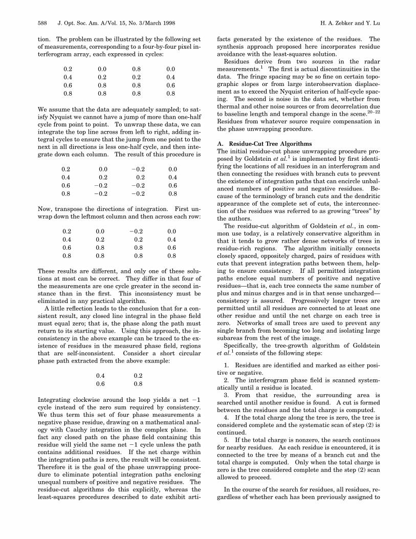
Fig. 1. Test data sets for algorithm intercomparison, in wrapped phase (raw interferogram) form. Two sets, (a) and (b), are simulateddata. One contains simple geometric shapes designed to illustrate the importance of residue distributions and proper tree locations, andone, derived from topographic data, includes layover and thermal noise. The box outlined in the lower left of the scene depicts addednoise. Actual data comprise two more scenes: (c) a very high signal-to-noise interferogram of a fairly flat area in Hawaii and (d) ruggedterrain in central California. Radar brightness appears as the intensity at each point and the phase as color, with one color cycle cor-responding to one fringe. (a) The simple geometrical target scene includes a pyramid structure that exhibits no phase discontinuities atits edges, a two-sided ramp structure that is continuous with the background on the left and right edges but discontinuous along the topand bottom, and a slanted wedge structure with exactly 2p phase change along its length. (b) The simulated topographic interferogramis most rugged in the upper left-hand corner, leading to significant layover in this area and less elsewhere. Scene (b) possesses a veryhigh fringe rate, scene (c) a moderate rate, and in scene (d) the background flat-Earth fringes have been removed.


Fig. 2. Phase errors after application of four unwrapping algorithms to the geometric-shape data set. (a) Results from the Goldsteinet al.1 residue-cut tree algorithm; only a one-cycle error on half of the wedge is generated. The rest of the image unwraps perfectly.Both the unweighted [(b)] and the weighted [(c)] least-squares algorithms exhibit large distortion fields associated with discontinuities atthe top and bottom of the ramp structure and from the half-wedge that showed the error in the tree case [(a)]. These results are iden-tical, as the weights assigned were unity everywhere (see text). The synthesis algorithm [(d)] produces the same result as the residue-cut algorithm here.

gorithm fails to return an answer. The mathematical de-scription of the algorithm is that of the individual partsdescribed in the sections above.

The accuracy of the synthesis algorithm, as in theleast-squares solution, depends on the appropriate choicefor the weights accorded each phase estimate. Zeroweight is assigned along the branch cuts of the residue-cut algorithm, and the remainder of the weights may beassigned according to correlation or signal strength aspreviously mentioned. We have found, though, that thegreatest gain in accuracy follows from the assignment ofthe zero weights on the cuts, and the other weights affectthe solution minimally.

It is also true that the synthesis algorithm will gener-ate errors if the branch cuts defining the zero weights areplaced in error. Unfortunately, no completely reliable al-gorithm for placing the weights has yet been demon-

strated. Simply balancing the number of positive andnegative residues along the cuts is an ambiguous methodof cut identification. The search for improved methods ofcut definition will have to continue if algorithms such asthose presented here are to be assuredly effective.

4. PERFORMANCE OF THE ALGORITHMSIn this section we illustrate the performance of the abovealgorithms in different phase unwrapping situations andcompose a table that summarizes the relative merits ofeach approach. We examine the accuracies achieved anderrors generated by several simple geometrical surfaceshapes, as well as interferograms generated by using to-pographic data and radar imaging geometries leading to


significant layover. We also inject noise into the simu-lated data to illustrate performance as a function ofsignal-to-noise level.

The performance of both phase unwrapping approacheshas been shown in the existing literature to be excellentin the case of high signal-to-noise ratio and continuous,adequately sampled underlying phase fields. In otherwords, these cases correspond to very low numbers ofresidues. We therefore skip the simple illustrations andproceed to cases in which the algorithms begin to fail.

We illustrate algorithms on several data sets, compris-ing simulated data, where we know the true unwrappedphase field, and also two sets of actual data where thetrue phases are unknown. In the former cases we calcu-late the errors explicitly, whereas for the latter we maystill examine the results visually and comment on algo-

rithm performance. The simulated data consist of twoscenes, one containing simple geometric shapes designedto illustrate the importance of residue distributions andproper tree locations and one derived from topographicdata. The topographic data scene has been used to con-struct a synthetic interferogram exhibiting layover, andthermal noise has been added in one region to demon-strate its deleterious affect. The real data also comprisetwo scenes, one a very high signal-to-noise interferogramof a fairly flat area in Hawaii acquired by NASA’s Space-borne Imaging Radar–C (SIR–C), which is straightfor-ward to unwrap by using all algorithms, and one of rug-ged terrain in Central California acquired by theEuropean Space Agency’s ERS–1 satellite. This seconddata set poses a challenge to all algorithms.

All four input interferograms are shown in wrapped

Fig. 3. Phase errors after application of four unwrapping algorithms to the synthetic topography data set. (a) Results from the Gold-stein et al.1 residue-cut tree algorithm. The algorithm fails to unwrap the heavily laid-over region in the upper-left and part of the noisyinset and also generates a few local one-cycle (2p) error regions. (b) The unweighted least-squares algorithm unwraps the image com-pletely but exhibits distortion associated with residues from layover and thermal noise. It also underestimates the overall slope of thescene from left to right. (c) The results from the weighted least-squares algorithm differs in detail but is similar. (d) The synthesisalgorithm produces a complete result much closer to the actual answer than the traditional least-squares approach, although errorsassociated with layover in the upper left and the noise in the box remain.


form in Fig. 1, where in each case we plot the radarbrightness as the intensity at each point and the phase ascolor. One color cycle corresponds to one fringe, so thatthe underlying fringe density may be compared. Thesimple geometrical target scene [Fig. 1(a)] includes apyramid structure that exhibits no phase discontinuitiesat its edges, a two-sided ramp structure that is continu-ous with the background on the left and right edges butdiscontinuous along the top and bottom, and a slantedwedge structure with exactly 2p phase change along itslength. We will see that this last target embodies an er-ror type that no existing algorithm can remove properly.

The simulated topographic interferogram [Fig. 1(b)] ismost rugged in the upper left-hand corner. We haveused an imaging geometry that generates significant lay-over in this area and less elsewhere. We have also addednoise to a box approximately one quarter the size of thescene so that we may compare performance in noisy andnoise-free regions—the box is visible and outlined in thelower left part of the image. For this image the signal-to-noise ratio in the box is 3 dB, and we examine the ef-fects of varying noise levels in a subsequent section below.The two actual data sets [Figs. 1(c) and 1(d)] are the Ha-waii and the California data, respectively, describedabove.

A. Error MagnitudesIn Fig. 2 we plot the phase errors after applying the fourunwrapping algorithms to the geometric-shape data set.Panel (a) shows the results from the Goldstein et al.1

residue-cut tree algorithm. The algorithm generatesonly a one-cycle error on half of the wedge, and the rest ofthe image unwraps perfectly. Since exactly 2p of phasechange occurs on the wedge, it is impossible to identifythe end that is continuous with the background in awrapped image. Consequently, no algorithm will resolvethis target properly. Similar structures are all too com-mon in real interferograms, so that there will always beimpossible unwrapping situations.

Both the unweighted [Fig. 2(b)] and the weighted [Fig.2(c)] least-squares algorithms generate large distortionfields emanating from discontinuities at the top and bot-tom of the ramp structure and from the half-wedge thatshowed the error in the tree case. These two algorithmsproduce identical results because the weights assignedwere unity everywhere. If appropriate weights had beenused, the results would have been superior in theweighted solution. These synthetic data are assumed tohave equal validity everywhere, leading to the choice ofunit weights in the weighted case. If data were known tobe on the edge of a discontinuity, reducing the weightshere would produce a less distorted result. This is whatthe synthesis algorithm is designed to do—identify pos-sible discontinuities and weight the least-squares solu-tion appropriately. The synthesis algorithm [Fig. 2(d)]produces the same result as the residue-cut algorithm forthis scene.

Figure 3 illustrates the difference between the un-wrapped estimates and the true phase values at eachpoint for the synthetic-topography data set. In this casealso we can calculate the actual error distribution, be-cause we know the original unwrapped solution. Again

panel (a) shows the results from the Goldstein et al.1

residue-cut tree algorithm. The algorithm fails to un-wrap the heavily laid-over region in the upper left andpart of the noisy inset and also generates a few local one-cycle (2p) error regions. The results are generally accu-rate, but incomplete, with the exceptions being a fewsmall parts of the laid-over and the noisy areas. The un-weighted least-squares algorithm [Fig. 3(b)] produces acomplete result but exhibits distortion associated withresidues generated by layover and thermal noise. It alsounderestimates the overall slope of the scene from left to

Fig. 4. Error signature of a dipole formed by a positive andnegative residue pair.

Table 1. Rms Errors from Four Algorithms

Region

RMS PhaseError (rad)

Goldsteinet al.1

UnweightedLeast-

Squares

WeightedLeast-

Squares Synthesis

Scene (a)Pyramid 0.000002a 0.000002a 0.000002a 0.000002a

Ramp 0.000002a 24.7 24.7 0.00002b

Wedge 1.07c 0.92c 0.92c 1.06c

Scene (b)Noise-free area

SNR: 1 0.827d 54.42 29.6 2.15SNR: 3 0.756d 22.05 17.3 2.15SNR: 10 0.744d 13.03 14.6 2.15SNR: 30 0.744d 12.74 14.5 2.15

Noisy areaSNR: 1 2.533d 35.01 200 2.57SNR: 3 1.282d 11.84 8.34 1.03SNR: 10 0.591d 4.48 6.14 0.32SNR: 30 0.543d 4.23 6.17 0.27

a Quantization noise only.b Errors along cuts only.c Half of wedge always one cycle (2p) off.d Includes only unwrapped area.


right. The results from the weighted least-squares [Fig.3(c)] differs in detail but is similar. Here we used thevalue of the interferogram correlation as the weight foreach point, and the correlation is assumed to be unity ev-erywhere except in the noise inset, where we calculate itfrom the signal-to-noise ratio following Zebker andVillasenor.21 The synthesis algorithm [Fig. 3(d)] pro-duces a complete result that is much closer to the actualanswer than with the traditional least-squares approach,although errors associated with layover in the upper leftand the noise in the box remain.

We calculate the root-mean-squared phase error forportions of these two synthetic data scenes and presentthe results for each of the four algorithms in Table 1. Forthe simple geometrical targets, we calculate the errorover the object itself plus a border around the object 30pixels in size so that the effect of discontinuities may becounted. For the synthetic topography scene, we calcu-late the errors in both the noise-free areas and the noiseregions independently. The noise-free areas are stillsubject to residues caused by layover. For the Goldstein

et al.1 case, we did not count the areas that did not un-wrap, so these numbers may be considered lower boundson the error.

We note that the Goldstein et al.1 algorithm performsquite well wherever it unwraps, with the single exceptionhere being the wedge feature. The wedge as chosen hereis ambiguous when shown in wrapped form, as it was de-vised to exhibit exactly one cycle of phase along its length.Thus when viewed as a wrapped data set, it appears con-tinuous at both ends against the background, whereas inreality only one end can be continuous. This situationcannot be unwrapped without prior knowledge as towhich end the discontinuity applies to, independent of thealgorithm chosen. In this particular case two residuesare found on the edges halfway along the target, leadingto a cut across the middle of the wedge. Thus half thewedge unwraps properly with this algorithm, and theother half is off by one cycle.

The least-squares approaches offer completeness of so-lution but at the cost of underestimating large-scaleslopes significantly. If we examine the error distribution

Fig. 5. Unwrapping of an easy scene, the Hawaii SIR-C data, by each of the four algorithms: (a) residue-cut trees, (b) unweightedleast-squares, (c) weighted least-squares, and (d) synthesis. All unwrap completely and get nearly the same result.


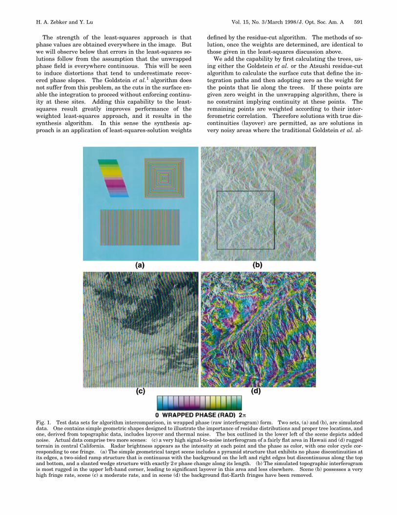
Fig. 6. Results of applying the four algorithms [(a) residue-cut trees, (b) unweighted least-squares, (c) weighted least-squares, and (d)synthesis] to a more difficult unwrapping problem, ERS-1 data over Parkfield, Calif. The residue-cut algorithm leaves significant gaps.Both of the least-squares algorithms produce subtly different results that significantly underestimate the tilt from upper left to lowerright in the scene. The synthesis algorithm gives a complete answer and recovers the global tilt accurately. There are undoubtedlyerrors of ;2p in magnitude in this solution, but they are not visible at this scale.

from the least-squares algorithm in greater detail, wenote that an interesting distortion pattern is producedfrom each pair of residues in the input image. Illus-trated in Fig. 4, the error signal radiates outward fromthe residue pair and is reminiscent of an electromagneticdipole pattern. The more-complex error fields found inthe more-complicated scenes are a combination of many ofthese individual dipole patterns. Therefore local discon-tinuities in the phase field generate residues and propa-gate errors throughout the image. These errors decaywith increasing distance from the residue dipole.

The weighted method outperformed the unweightedmethod for the noisy region in cases of high noise and isuseful if we know the location of the noisy area and setthe weighting value in this area to be relatively low. Forthose areas with discontinuities, the results are poor be-cause of the least-squares algorithm property to tend to

smooth out the solution to make it everywhere continu-ous. Therefore this method works poorly for the layoverregion. But if we know the location of jumps and we setthe weighting values equal to zero at those discontinui-ties, we can get a reasonably good solution. Once again,the shortcoming of the existing least-squares algorithm isin the choice of proper weights, not in any mathematicallimitations of the approach.

Other techniques for generating zero weights alongcuts have been examined. One approach is to thresholdthe correlation coefficients so that values below some cut-off are set equal to zero. This method works in laid-overregions, which tend to have low correlation. It will, how-ever, miss placing cuts along cliffs oriented perpendicularto the flight path, as well as areas where a phase discon-tinuity is a result of certain ground motions between in-terferometric observations. These cases are identified by


using the synthesis algorithm, which generates weightswithout any additional knowledge of the scene character-istics.

Figures 5 and 6 present the results of applying all fouralgorithms to the Hawaii (Fig. 5) and the California (Fig.6) data. The Hawaii data set unwraps well in all fourcases. But in the case of the California data, the Goldsteinet al.1 algorithm leaves significant gaps in coverage. Theunweighted and weighted least-squares algorithms givecomplete coverage but do not match the overall slope asseen in the Goldstein et al. result. Only the synthesis al-gorithm yields full coverage plus the correct image tilt.

B. Computational EfficiencyIn addition to accuracy, computation time is important forall applications requiring moderate to high throughput.In Table 2 we give the time required on our Hewlett–Packard 712 workstation for each of the four scenes, forthe Goldstein et al.1 unweighted least-squares, weightedleast-squares, and synthesis algorithms. The variationamong algorithms is quite large, ranging from 2.7 to1844.5 s. The synthesis algorithm is by far the least ef-ficient on synthetic data but is comparable to weightedleast-squares for real data. It is likely that optimizingthe convergence criterion could lead to a drastic reductionin execution time for the weighted least-squares and syn-thesis approaches.

Table 2. Computational Efficiencies of theAlgorithms

Scene

Execution Time (s)

Goldsteinet al.1

UnweightedLeast-

Squares

WeightedLeast-

Squares Synthesis

A. Geometricaltargets

12.9 19.7 19.7 1223.0

B. SynthetictopographySNR: 1 7.2 18.9 225.1 1337.1SNR: 3 5.2 19.0 224.5 1240.0SNR: 10 9.0 18.9 224.3 939.7SNR: 30 5.9 19.7 224.8 949.3

C. Hawaii 2.7 18.8 1844.5a 306.1D. California 3.2 18.8 231.8 211.7

a Hawaii scene converged with 10210 error after approximately 2 min.Continuing until 10212 required 30 min.

Table 3. Summary of Algorithm Intercomparisons

Algorithm Coverage Accuracy Efficiency

Goldstein et al. Limited Excellent FastUnweighted least-

squaresComplete Much distortion

if many residuesexist

Moderate

Weighted least-squares

Complete Can be better thanunweighted

Slow

Synthesis Complete Good/Excellent Slow

5. CONCLUSIONSTable 3 summarizes the comparison of the four algo-rithms that we examined in this paper: the Goldsteinet al.1 algorithm, the unweighted least-squares algo-rithm, the weighted least-squares algorithm, and the syn-thesis algorithm. The conservative Goldstein et al. algo-rithm is fast and gives accurate results where it canunwrap. Errors inherent in certain singular cases suchas the 2p wedge shown above are unwrapped in error byall algorithms. The algorithm is limited to areas of mod-erate residue density.

The unweighted least-squares algorithm also is reason-ably efficient but performs poorly in all but the most be-nign situations. A significant improvement is affordedby using weighted algorithms, although a large penalty incomputational time is incurred. Substituting weightedfor unweighted solutions would be a useful trade-off foranalysis of a very few interferograms.

A synthesis algorithm that combines the integrationpath isolation of the residue-cut methods with the betternoise-region performance of the least-squares algorithmsyields the greatest coverage with least error. However, itsuffers from the same computational complexity that af-fects the weighted least-squares algorithm. Nonethelessit remains the most accurate and complete method avail-able. Algorithm improvements, along with increases inthe speed of inexpensive computers, may in time amelio-rate this problem.

Phase unwrapping remains a significant issue in radarinterferometry. Particularly for cases involving largeamounts of data to be processed, the issue will requirefurther study. However, for scientific analysis of a lim-ited number of interferograms, the algorithms presentedhere may be usefully employed.

Correspondence should be sent to Howard A. Zebker,tel: 650-723-8067; fax: 650-725-7344; e-mail: [email protected].

REFERENCES1. R. M. Goldstein, H. A. Zebker, and C. Werner, ‘‘Satellite ra-

dar interferometry: two-dimensional phase unwrapping,’’Radio Sci. 23, 713–720 (1988).

2. D. C. Ghiglia and L. A. Romero, ‘‘Robust two-dimensionalweighted and unweighted phase unwrapping that uses fasttransforms and iterative methods, ’’ J. Opt. Soc. Am. A 11,107–117 (1994).

3. M. D. Pritt and J. S. Shipman, ‘‘Least-squares two-dimensional phase unwrapping using FFT’s,’’ IEEE Trans.Geosci. Remote Sens. 32, 706–708 (1994).

4. G. Fornaro, G. Franceschetti, and R. Lanari, ‘‘Interferomet-ric SAR phase unwrapping using Green’s formulation,’’IEEE Trans. Geosci. Remote Sens. 34, 720–727 (1996).

5. H. Zebker and R. Goldstein, ‘‘Topographic mapping from in-terferometric SAR observations,’’ J. Geophys. Res. 91,4993–4999 (1986).

6. H. A. Zebker, T. G. Farr, R. P. Salazar, and T. H. Dixon,‘‘Mapping the world’s topography using radar interferom-etry: the TOPSAT mission,’’ Proc. IEEE 82, 1774–1786(1994).

7. A. K. Gabriel, R. M. Goldstein, and H. A. Zebker, ‘‘Mappingsmall elevation changes over large areas: differential ra-dar interferometry, ’’ J. Geophys. Res. 94, 9183–9191(1989).

8. D. Massonnet, M. Rossi, C. Carmona, F. Adragna, G.


Peltzer, K. Feigl, and T. Rabaute, ‘‘The displacement field ofthe Landers earthquake mapped by radar interferometry,’’Nature (London) 364, 138–142 (1993).

9. H. A. Zebker, P. A. Rosen, R. M. Goldstein, A. Gabriel, andC. Werner, ‘‘On the derivation of coseismic displacementfields using differential radar interferometry: the Landersearthquake,’’ J. Geophys. Res. 99, 19617–19634 (1994).

10. R. M. Goldstein and H. A. Zebker, ‘‘Interferometric radarmeasurement of ocean surface currents,’’ Nature (London)328, 707–709 (1987).

11. R. M. Goldstein, H. Engelhardt, B. Kamb, and R. M.Frolich, ‘‘Satellite radar interferometry for monitoring icesheet motion: application to an Antarctic ice stream,’’ Sci-ence 262, 1525–1530 (1993).

12. S. N. Madsen, J. Martin, and H. A. Zebker, ‘‘Analysis andevaluation of the NASA/JPL TOPSAR interferometric SARsystem,’’ IEEE Trans. Geosci. Remote Sens. 33, 383–391(1995).

13. D. Massonnet, K. Feigl, M. Rossi, and F. Adragna, ‘‘Radarinterferometric mapping of deformation in the year afterthe Landers earthquake,’’ Nature (London) 369, 227–230(1994).

14. D. Massonnet and K. L. Feigl, ‘‘Discrimination of geophys-ical phenomena in satellite radar interferograms,’’ Geo-phys. Res. Lett. 22, 1537–1540 (1995).

15. H. A. Zebker, C. L. Werner, P. Rosen, and S. Hensley, ‘‘Ac-

curacy of topographic maps derived from ERS-1 radar in-terferometry,’’ IEEE Trans. Geosci. Remote Sens. 32, 823–836 (1994).

16. G. Fornaro, G. Franceschetti, R. Lanari, and E. Sansoti,‘‘Robust phase unwrapping techniques: a comparison,’’ J.Opt. Soc. Am. A 13, 2355–2366 (1996).

17. M. D. Pritt, ‘‘Phase unwrapping by means of multigrid tech-niques for interferometric SAR,’’ IEEE Trans. Geosci. Re-mote Sens. 34, 728–738 (1996).

18. D. J. Bone, ‘‘Fourier fringe analysis: the two-dimensionalphase unwrapping problem,’’ Appl. Opt. 30, 3627–32(1991).

19. A. Collaro, G. Franceschetti, F. Palmieri, and M. S. Fer-reiro, ‘‘Phase unwrapping by means of genetic algorithms,’’J. Opt. Soc. Am. A 15, 407–418 (1997).

20. E. Rodriguez and J. Martin, ‘‘Theory and design of inter-ferometric SARs,’’ Proc. IEEE 139, 147–159 (1992).

21. H. A. Zebker and J. Villasenor, ‘‘Decorrelation in interfero-metric radar echoes,’’ IEEE Trans. Geosci. Remote Sens.30, 950–959 (1992).

22. F. Li and R. M. Goldstein, ‘‘Studies of multi-baseline space-borne interferometric synthetic aperture radars,’’ IEEETrans. Geosci. Remote Sens. 28, 88–97 (1990).

23. B. R. Hunt, ‘‘Matrix formulation of the reconstruction ofphase values from phase differences,’’ J. Opt. Soc. Am. 69,393–399 (1979).

Phase unwrapping algorithms for radar interferometry...

Documents

Transcript of Phase unwrapping algorithms for radar interferometry...