Phase Retrieval via Wirtinger Flow: Theory and Algorithms

Emmanuel J. Candes∗ Xiaodong Li† Mahdi Soltanolkotabi‡

July 3, 2014; Revised January 2015

Abstract

We study the problem of recovering the phase from magnitude measurements; specifically, wewish to reconstruct a complex-valued signal x ∈ Cn about which we have phaseless samples of theform yr = ∣⟨ar,x⟩∣

2, r = 1, . . . ,m (knowledge of the phase of these samples would yield a linear

system). This paper develops a non-convex formulation of the phase retrieval problem as wellas a concrete solution algorithm. In a nutshell, this algorithm starts with a careful initializationobtained by means of a spectral method, and then refines this initial estimate by iterativelyapplying novel update rules, which have low computational complexity, much like in a gradientdescent scheme. The main contribution is that this algorithm is shown to rigorously allow theexact retrieval of phase information from a nearly minimal number of random measurements.Indeed, the sequence of successive iterates provably converges to the solution at a geometric rateso that the proposed scheme is efficient both in terms of computational and data resources. Intheory, a variation on this scheme leads to a near-linear time algorithm for a physically realizablemodel based on coded diffraction patterns. We illustrate the effectiveness of our methods withvarious experiments on image data. Underlying our analysis are insights for the analysis of non-convex optimization schemes that may have implications for computational problems beyondphase retrieval.

1 Introduction

We are interested in solving quadratic equations of the form

yr = ∣⟨ar,z⟩∣2 , r = 1,2, . . . ,m, (1.1)

where z ∈ Cn is the decision variable, ar ∈ Cn are known sampling vectors, and yr ∈ R are observedmeasurements. This problem is a general instance of a nonconvex quadratic program (QP). Noncon-vex QPs have been observed to occur frequently in science and engineering and, consequently, theirstudy is of importance. For example, a class of combinatorial optimization problems with Booleandecision variables may be cast as QPs [52, Section 4.3.1]. Focusing on the literature on physicalsciences, the problem (1.1) is generally referred to as the phase retrieval problem. To understandthis connection, recall that most detectors can only record the intensity of the light field and notits phase. Thus, when a small object is illuminated by a quasi-monochromatic wave, detectorsmeasure the magnitude of the diffracted light. In the far field, the diffraction pattern happens to

∗Departments of Mathematics and of Statistics, Stanford University, Stanford CA†Department of Statistics, The Wharton School, University of Pennsylvania, Philadelphia, PA‡Ming Hsieh Department of Electrical Engineering, University of Southern California, Los Angeles, CA

1

be the Fourier transform of the object of interest—this is called Fraunhofer diffraction—so that indiscrete space, (1.1) models the data aquisition mechanism in a coherent diffraction imaging setup;one can identify z with the object of interest, ar with complex sinusoids, and yr with the recordeddata. Hence, we can think of (1.1) as a generalized phase retrieval problem. As is well known, thephase retrieval problem arises in many areas of science and engineering such as X-ray crystallogra-phy [33,48], microscopy [47], astronomy [21], diffraction and array imaging [12,18], and optics [66].Other fields of application include acoustics [4, 5], blind channel estimation in wireless communi-cations [3, 58], interferometry [22], quantum mechanics [20, 59] and quantum information [35]. Werefer the reader to the tutorial paper [62] for a recent review of the theory and practice of phaseretrieval.

Because of the practical significance of the phase retrieval problem in imaging science, thecommunity has developed methods for recovering a signal x ∈ Cn from data of the form yr = ∣⟨ar,x⟩∣2

in the special case where one samples the (square) modulus of its Fourier transform. In this setup,the most widely used method is perhaps the error reduction algorithm and its generalizations,which were derived from the pioneering research of Gerchberg and Saxton [29] and Fienup [24,26].The Gerchberg-Saxton algorithm starts from a random initial estimate and proceeds by iterativelyapplying a pair of ‘projections’: at each iteration, the current guess is projected in data space sothat the magnitude of its frequency spectrum matches the observations; the signal is then projectedin signal space to conform to some a-priori knowledge about its structure. In a typical instance,our knowledge may be that the signal is real-valued, nonnegative and spatially limited. First,while error reduction methods often work well in practice, the algorithms seem to rely heavilyon a priori information about the signals, see [25, 27, 34, 60]. Second, since these algorithms canbe cast as alternating projections onto nonconvex sets [8] (the constraint in Fourier space is notconvex), fundamental mathematical questions concerning their convergence remain, for the mostpart, unresolved; we refer to Section 3.2 for further discussion.

On the theoretical side, several combinatorial optimization problems—optimization programswith discrete design variables which take on integer or Boolean values—can be cast as solvingquadratic equations or as minimizing a linear objective subject to quadratic inequalities. In theirmost general form these problems are known to be notoriously difficult (NP-hard) [52, Section 4.3].Nevertheless, many heuristics have been developed for addressing such problems.1 One popularheuristic is based on a class of convex relaxations known as Shor’s relaxations [52, Section 4.3.1]which can be solved using tractable semi-definite programming (SDP). For certain random models,some recent SDP relaxations such as PhaseLift [14] are known to provide exact solutions (up toglobal phase) to the generalized phase retrieval problem using a near minimal number of samplingvectors [16, 17]. While in principle SDP based relaxations offer tractable solutions, they becomecomputationally prohibitive as the dimension of the signal increases. Indeed, for a large number ofunknowns in the tens of thousands, say, the memory requirements are far out of reach of desktopcomputers so that these SDP relaxations are de facto impractical.

2 Algorithm: Wirtinger Flow

This paper introduces an approach to phase retrieval based on non-convex optimization as well asa solution algorithm, which has two components: (1) a careful initialization obtained by means of

1For a partial review of some of these heuristics as well as some recent theoretical advances in related problems werefer to our companion paper [16, Section 1.6] and references therein [7, 13,30,31,36,55,56,65].

2

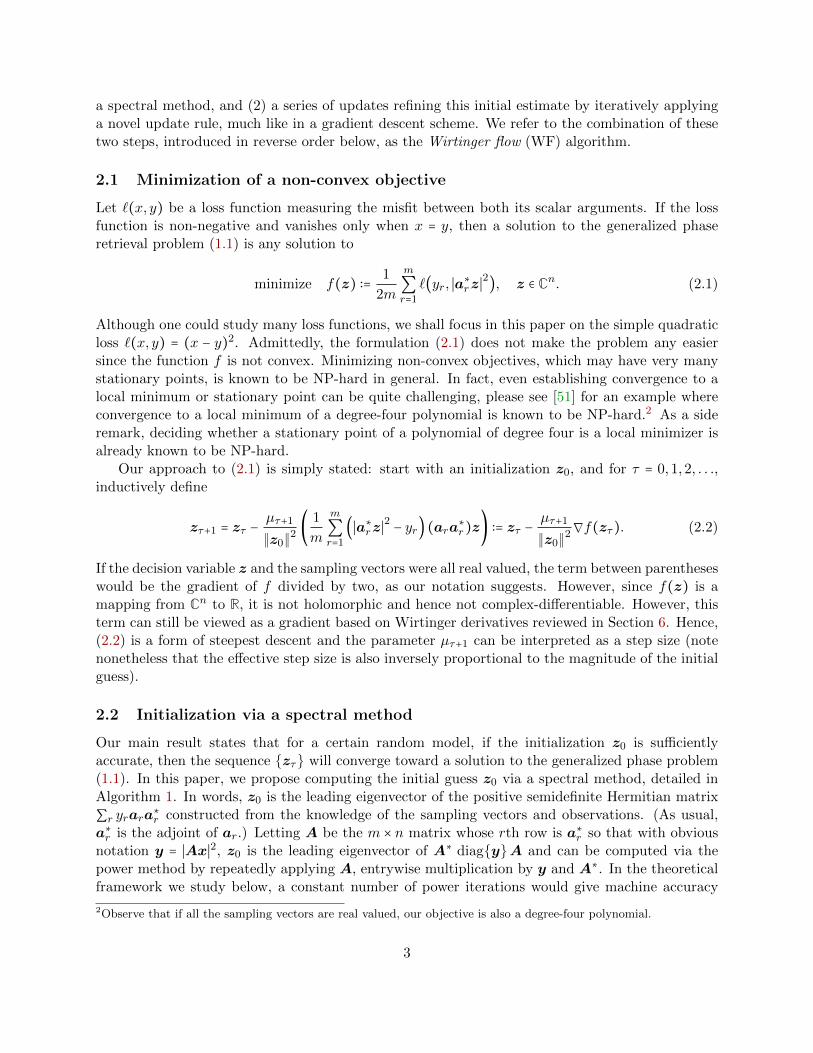
a spectral method, and (2) a series of updates refining this initial estimate by iteratively applyinga novel update rule, much like in a gradient descent scheme. We refer to the combination of thesetwo steps, introduced in reverse order below, as the Wirtinger flow (WF) algorithm.

2.1 Minimization of a non-convex objective

Let `(x, y) be a loss function measuring the misfit between both its scalar arguments. If the lossfunction is non-negative and vanishes only when x = y, then a solution to the generalized phaseretrieval problem (1.1) is any solution to

minimize f(z) ∶=1

2m

m

∑r=1

`(yr, ∣a∗rz∣

2), z ∈ Cn. (2.1)

Although one could study many loss functions, we shall focus in this paper on the simple quadraticloss `(x, y) = (x − y)2. Admittedly, the formulation (2.1) does not make the problem any easiersince the function f is not convex. Minimizing non-convex objectives, which may have very manystationary points, is known to be NP-hard in general. In fact, even establishing convergence to alocal minimum or stationary point can be quite challenging, please see [51] for an example whereconvergence to a local minimum of a degree-four polynomial is known to be NP-hard.2 As a sideremark, deciding whether a stationary point of a polynomial of degree four is a local minimizer isalready known to be NP-hard.

Our approach to (2.1) is simply stated: start with an initialization z0, and for τ = 0,1,2, . . .,inductively define

zτ+1 = zτ −µτ+1

∥z0∥2(

1

m

m

∑r=1

(∣a∗rz∣2− yr) (ara

∗r)z) ∶= zτ −

µτ+1

∥z0∥2∇f(zτ). (2.2)

If the decision variable z and the sampling vectors were all real valued, the term between parentheseswould be the gradient of f divided by two, as our notation suggests. However, since f(z) is amapping from Cn to R, it is not holomorphic and hence not complex-differentiable. However, thisterm can still be viewed as a gradient based on Wirtinger derivatives reviewed in Section 6. Hence,(2.2) is a form of steepest descent and the parameter µτ+1 can be interpreted as a step size (notenonetheless that the effective step size is also inversely proportional to the magnitude of the initialguess).

2.2 Initialization via a spectral method

Our main result states that for a certain random model, if the initialization z0 is sufficientlyaccurate, then the sequence {zτ} will converge toward a solution to the generalized phase problem(1.1). In this paper, we propose computing the initial guess z0 via a spectral method, detailed inAlgorithm 1. In words, z0 is the leading eigenvector of the positive semidefinite Hermitian matrix

∑r yrara∗r constructed from the knowledge of the sampling vectors and observations. (As usual,

a∗r is the adjoint of ar.) Letting A be the m × n matrix whose rth row is a∗r so that with obviousnotation y = ∣Ax∣2, z0 is the leading eigenvector of A∗ diag{y}A and can be computed via thepower method by repeatedly applying A, entrywise multiplication by y and A∗. In the theoreticalframework we study below, a constant number of power iterations would give machine accuracy

2Observe that if all the sampling vectors are real valued, our objective is also a degree-four polynomial.

3

because of an eigenvalue gap between the top two eigenvalues, please see Appendix B for additionalinformation.

Algorithm 1 Wirtinger Flow: Initialization

Input: Observations {yr} ∈ Rm.Set

λ2= n

∑r yr

∑r ∥ar∥2.

Set z0, normalized to ∥z0∥ = λ, to be the eigenvector corresponding to the largest eigenvalue of

Y =1

m

m

∑r=1

yrara∗r .

Output: Initial guess z0.

2.3 Wirtinger flow as a stochastic gradient scheme

We would like to motivate the Wirtinger flow algorithm and provide some insight as to why weexpect it to work in a model where the sampling vectors are random. First, we emphasize thatour statements in this section are heuristic in nature; as it will become clear in the proof Section7, a correct mathematical formalization of these ideas is far more complicated than our heuristicdevelopment here may suggest. Second, although our ideas are broadly applicable, it makes senseto begin understanding the algorithm in a setting where everything is real valued, and in which thevectors ar are i.i.d. N (0,I). Also without any loss in generality and to simplify exposition in thissection we shall assume ∥x∥ = 1.

Let x be a solution to (1.1) so that yr = ∣⟨ar,x⟩∣2, and consider the initialization step first. Inthe Gaussian model, a simple moment calculation gives

E [1

m

m

∑r=1

yrara∗r] = I + 2xx∗.

By the strong law of large numbers, the matrix Y in Algorithm 1 is equal to the right-hand sidein the limit of large samples. Since any leading eigenvector of I + 2xx∗ is of the form λx for somescalar λ ∈ R, we see that the intialization step would recover x perfectly, up to a global sign orphase factor, had we infinitely many samples. Indeed, the chosen normalization would guaranteethat the recovered signal is of the form ±x. As an aside, we would like to note that the top twoeigenvalues of I + 2xx∗ are well separated unless ∥x∥ is very small, and that their ratio is equalto 1 + 2∥x∥2. Now with a finite amount of data, the leading eigenvector of Y will of course not beperfectly correlated with x but we hope that it is sufficiently correlated to point us in the rightdirection.

We now turn our attention to the gradient-update (2.2) and define

F (z) = z∗(I −xx∗)z +3

4(∥z∥2

− 1)2,

where here and below, x is once again our planted solution. The first term ensures that thedirection of z matches the direction of x and the second term penalizes the deviation of the

4

Euclidean norm of z from that of x. Obviously, the minimizers of this function are ±x. Nowconsider the gradient scheme

zτ+1 = zτ −µτ+1

∥z0∥2∇F (zτ). (2.3)

In Section 7.9, we show that if min ∥z0 ±x∥ ≤ 1/8 ∥x∥, then {zτ} converges to x up to a globalsign. However, this is all ideal as we would need knowledge of x itself to compute the gradient ofF ; we simply cannot run this algorithm.

Consider now the WF update and assume for a moment that zτ is fixed and independent of thesampling vectors. We are well aware that this is a false assumption but nevertheless wish to exploresome of its consequences. In the Gaussian model, if z is independent of the sampling vectors, thena modification of Lemma 7.2 for real-valued z shows that E[∇f(z)] = ∇F (z) and, therefore,

E[zτ+1] = E[zτ ] −µτ+1

∥z0∥2

E[∇f(zτ)] ⇒ E[zτ+1] = zτ −µτ+1

∥z0∥2∇F (zτ).

Hence, the average WF update is the same as that in (2.3) so that we can interpret the Wirtingerflow algorithm as a stochastic gradient scheme in which we only get to observe an unbiased estimate∇f(z) of the “true” gradient ∇F (z).

Regarding WF as a stochastic gradient scheme helps us in choosing the learning parameter orstep size µτ . Lemma 7.7 asserts that

∥∇f(z) −∇F (z)∥2≤ ∥x∥

2⋅min ∥z ±x∥ (2.4)

holds with high probability. Looking at the right-hand side, this says that the uncertainty aboutthe gradient estimate depends on how far we are from the actual solution x. The further away,the larger the uncertainty or the noisier the estimate. This suggests that in the early iterationswe should use a small learning parameter as the noise is large since we are not yet close to thesolution. However, as the iterations count increases and we make progress, the size of the noise alsodecreases and we can pick larger values for the learning parameter. This heuristic together withexperimentation lead us to consider

µτ = min(1 − e−τ/τ0 , µmax) (2.5)

shown in Figure 1. Values of τ0 around 330 and of µmax around 0.4 worked well in our simulations.This makes sure that µτ is rather small at the beginning (e.g. µ1 ≈ 0.003 but quickly increases andreaches a maximum value of about 0.4 after 200 iterations or so.

3 Main Results

3.1 Exact phase retrieval via Wirtinger flow

Our main result establishes the correctness of the Wirtinger flow algorithm in the Gaussian modeldefined below. Later in Section 5, we shall also develop exact recovery results for a physicallyinspired diffraction model.

Definition 3.1 We say that the sampling vectors follow the Gaussian model if ar ∈ Cn i.i.d.∼ N (0,I/2)+

iN (0,I/2). In the real-valued case, they are i.i.d. N (0,I).

5

0 50 100 150 200 250 300

0

0.1

0.2

0.3

0.4

τµτ

Figure 1: Learning parameter µτ from (2.5) as a function of the iteration count τ ;here, τ0 ≈ 330 and µmax = 0.4.

We also need to define the distance to the solution set.

Definition 3.2 Let x ∈ Cn be any solution to the quadratic system (1.1) (the signal we wish torecover). For each z ∈ Cn, define

dist(z,x) = minφ∈[0,2π]

∥z − eiφx∥ .

Theorem 3.3 Let x be an arbitrary vector in Cn and y = ∣Ax∣2 ∈ Rm be m quadratic samples withm ≥ c0 ⋅ n logn, where c0 is a sufficiently large numerical constant. Then the Wirtinger flow initialestimate z0 normalized to have squared Euclidean norm equal to m−1

∑r yr,3 obeys

dist(z0,x) ≤1

8∥x∥ (3.1)

with probability at least 1− 10e−γn − 8/n2 (γ is a fixed positive numerical constant). Further, take aconstant learning parameter sequence, µτ = µ for all τ = 1,2, . . . and assume µ ≤ c1/n for some fixednumerical constant c1. Then there is an event of probability at least 1 − 13e−γn −me−1.5m − 8/n2,such that on this event, starting from any initial solution z0 obeying (3.1), we have

dist(zτ ,x) ≤1

8(1 −

µ

4)τ/2

⋅ ∥x∥ .

Clearly, one would need 2n quadratic measurements to have any hope of recovering x ∈ Cn. Itis also known that in our sampling model, the mapping z ↦ ∣Az∣2 is injective for m ≥ 4n [5] andthat this property holds for generic sampling vectors [19].4 Hence, the Wirtinger flow algorithmloses at most a logarithmic factor in the sampling complexity. In comparison, the SDP relaxationonly needs a sampling complexity proportional to n (no logarithmic factor) [15], and it is an openquestion whether Theorem 3.3 holds in this regime.

3The same results holds with the intialization from Algorithm 1 because ∑r ∥ar∥2≈ m ⋅ n with a standard deviation

of about the square root of this quantity.4It is not within the scope of this paper to explain the meaning of generic vectors and, instead, refer the interestedreader to [19].

6

Setting µ = c1/n yields ε accuracy in a relative sense, namely, dist(z,x) ≤ ε ∥x∥, in O(n log 1/ε)iterations. The computational work at each iteration is dominated by two matrix-vector productsof the form Az and A∗v, see Appendix B. It follows that the overall computational complexity ofthe WF algorithm is O(mn2 log 1/ε). Later in the paper, we will exhibit a modification to the WFalgorithm of mere theoretical interest, which also yields exact recovery under the same samplingcomplexity and an O(mn log 1/ε) computational complexity; that is to say, the computationalworkload is now just linear in the problem size.

3.2 Comparison with other non-convex schemes

We now pause to comment on a few other non-convex schemes in the literature. Other comparisonsmay be found in our companion paper [16].

Earlier, we discussed the Gerchberg-Saxton and Fienup algorithms. These formulations assumethat A is a Fourier transform and can be described as follows: suppose zτ is the current guess,then one computes the image of zτ through A and adjust its modulus so that it matches that ofthe observed data vector: with obvious notation,

vτ+1 = b⊙Azτ∣Azτ ∣

, (3.2)

where ⊙ is elementwise multiplication, and b = ∣Ax∣ so that b2r = yr for all r = 1, . . . ,m. Then

vτ+1 = arg minv∈Cn ∥vτ+1 −Av∥. (3.3)

(In the case of Fourier data, the step (3.2)–(3.3) essentially adjusts the modulus of the Fouriertransform of the current guess so that it fits the measured data.) Finally, if we know that thesolution belongs to a convex set C (as in the case where the signal is known to be real-valued,possibly non-negative and of finite support), then the next iterate is

zτ+1 = PC(vτ+1), (3.4)

where PC is the projection onto the convex set C. If no such information is available, then zτ+1 =

vτ+1. The first step (3.3) is not a projection onto a convex set and, therefore, it is in generalcompletely unclear whether the Gerchberg-Saxton algorithm actually converges. (And if it were toconverge, at what speed?) It is also unclear how the procedure should be initialized to yield accuratefinal estimates. This is in contrast to the Wirtinger flow algorithm, which in the Gaussian modelis shown to exhibit geometric convergence to the solution to the phase retrieval problem. Anotherbenefit is that the Wirtinger flow algorithm does not require solving a least-squares problem (3.3)at each iteration; each step enjoys a reduced computational complexity.

A recent contribution related to ours is the interesting paper [54], which proposes an alternatingminimization scheme named AltMinPhase for the general phase retrieval problem. AltMinPhaseis inspired by the Gerchberg-Saxton update (3.2)–(3.3) as well as other established alternatingprojection heuristics [26, 42, 43, 45, 46, 67]. We describe the algorithm in the setup of Theorem3.3 for which [54] gives theoretical guarantees. To begin with, AltMinPhase partitions the sam-pling vectors ar (the rows of the matrix A) and corresponding observations yr into B + 1 disjointblocks (y(0),A(0)), (y(1),A(1)), . . ., (y(B),A(B)) of roughly equal size. Hence, distinct blocks arestochastically independent from each other. The first block (y(0),A(0)) is used to compute aninitial estimate z0. After initialization, AltMinPhase goes through a series of iterations of the form

7

(3.2)–(3.3), however, with the key difference that each iteration uses a fresh set of sampling vectorsand observations: in details,

zτ+1 = arg minz∈Cn ∥vτ+1 −A(τ+1)z∥, vτ+1 = b⊙A(τ+1)zτ

∣A(τ+1)zτ ∣. (3.5)

As for the Gerchberg-Saxton algorithm, each iteration requires solving a least-squares problem.Now assume a real-valued Gaussian model as well as a real valued solution x ∈ Rn. The mainresult in [54] states that if the first block (y(0),A(0)) contains at least c ⋅n log3 n samples and eachconsecutive block contains at least c ⋅n logn samples—c here denotes a positive numerical constantwhose value may change at each occurence—then it is possible to initialize the algorithm via datafrom the first block in such a way that each consecutive iterate (3.5) decreases the error ∥zτ −x∥ by50%; naturally, all of this holds in a probabilistic sense. Hence, one can get ε accuracy in the senseintroduced earlier from a total of c ⋅ n logn ⋅ (log2 n + log 1/ε) samples. Whereas the Wirtinger flowalgorithm achieves arbitrary accuracy from just c ⋅ n logn samples, these theoretical results wouldrequire an infinite number of samples. This is, however, not the main point.

The main point is that in practice, it is not realistic to imagine (1) that we will divide thesamples in distinct blocks (how many blocks should we form a priori? of which sizes?) and (2) thatwe will use measured data only once. With respect to the latter, observe that the Gerchberg-Saxtonprocedure (3.2)–(3.3) uses all the samples at each iteration. This is the reason why AltMinPhase is oflittle practical value, and of theoretical interest only. As a matter of fact, its design and study seemmerely to stem from analytical considerations: since one uses an independent set of measurementsat each iteration, A(τ+1) and zτ are stochastically independent, a fact which considerably simplifiesthe convergence analysis. In stark contrast, the WF iterate uses all the samples at each iterationand thus introduces some dependencies, which makes for some delicate analysis. Overcomingthese difficulties is crucial because the community is preoccupied with convergence properties ofalgorithms one actually runs, like Gerchberg-Saxton (3.2)–(3.3), or would actually want to run.Interestingly, it may be possible to use some of the ideas developed in this paper to develop arigorous theory of convergence for algorithms in the style of Gerchberg-Saxton and Fienup, pleasesee [63].

In a recent paper [44], which appeared on the arXiv preprint server as the final version of thispaper was under preparation, the authors explore necessary and sufficient conditions for the globalconvergence of an alternative minimization scheme with generic sampling vectors. The issue isthat we do not know when these conditions hold. Further, even when the algorithm converges,it does not come with an explicit convergence rate so that is is not known whether the algorithmconverges in polynomial time. As before, some of our methods as well as those from our companionpaper [16] may have some bearing upon the analysis of this algorithm. Similarly, another class ofnonconvex algorithms that have recently been proposed in the literature are iterative algorithmsbased on Generalized Approximate Message Passing (GAMP), see [57] and [61] as well as [9,10,23]for some background literature on AMP. In [61], the authors demonstrate a favorable runtime foran algorithm of this nature. However, this does not come with any theoretical guarantees.

Moving away from the phase retrieval problem, we would like to mention some very interestingwork on the matrix completion problem using non-convex schemes by Montanari and coauthors[38–40], see also [2,6,32,37,41,49,50]. Although the problems and models are quite different, thereare some general similarities between the algorithm named OptSpace in [39] and ours. Indeed,OptSpace operates by computing an initial guess of the solution to a low-rank matrix completion

8

problem by means of a spectral method. It then sets up a nonconvex problem, and proposes aniterative algorithm for solving it. Under suitable assumptions, [39] demonstrates the correctness ofthis method in the sense that OptSpace will eventually converge to a low-rank solution, althoughit is not shown to converge in polynomial time.

4 Numerical Experiments

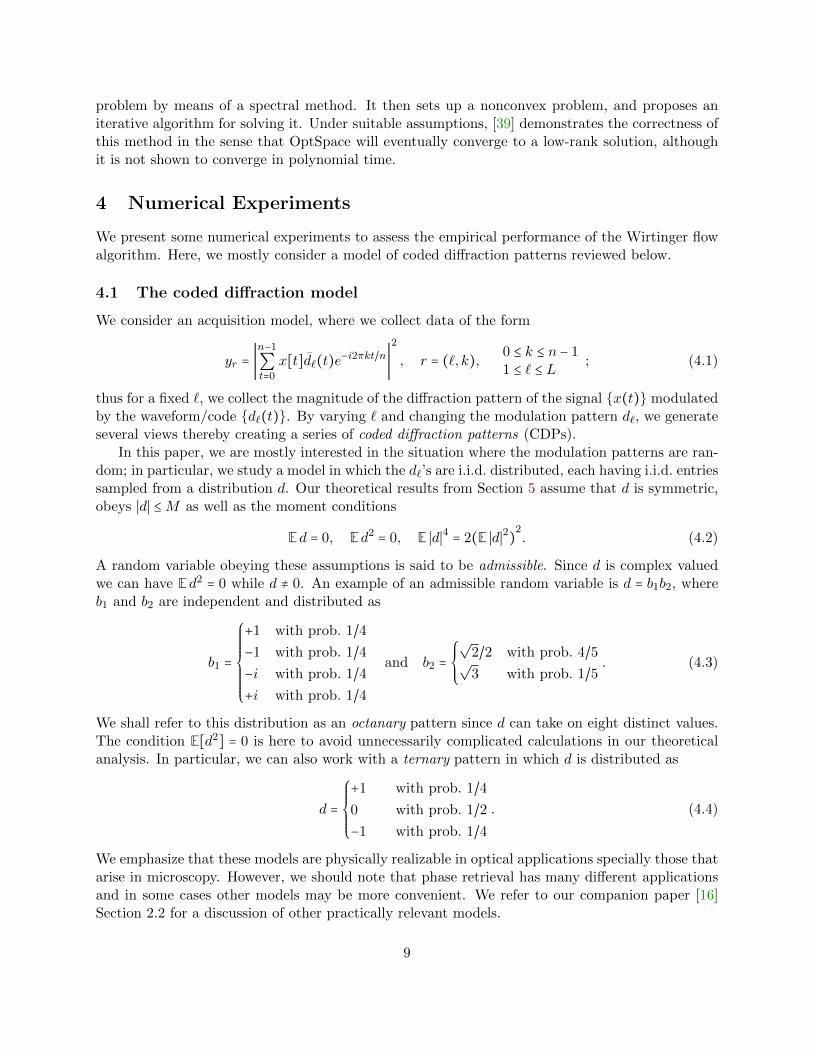
We present some numerical experiments to assess the empirical performance of the Wirtinger flowalgorithm. Here, we mostly consider a model of coded diffraction patterns reviewed below.

4.1 The coded diffraction model

We consider an acquisition model, where we collect data of the form

yr = ∣n−1

∑t=0

x[t]d`(t)e−i2πkt/n

∣

2

, r = (`, k),0 ≤ k ≤ n − 11 ≤ ` ≤ L

; (4.1)

thus for a fixed `, we collect the magnitude of the diffraction pattern of the signal {x(t)} modulatedby the waveform/code {d`(t)}. By varying ` and changing the modulation pattern d`, we generateseveral views thereby creating a series of coded diffraction patterns (CDPs).

In this paper, we are mostly interested in the situation where the modulation patterns are ran-dom; in particular, we study a model in which the d`’s are i.i.d. distributed, each having i.i.d. entriessampled from a distribution d. Our theoretical results from Section 5 assume that d is symmetric,obeys ∣d∣ ≤M as well as the moment conditions

Ed = 0, Ed2= 0, E ∣d∣4 = 2(E ∣d∣2)

2. (4.2)

A random variable obeying these assumptions is said to be admissible. Since d is complex valuedwe can have Ed2 = 0 while d ≠ 0. An example of an admissible random variable is d = b1b2, whereb1 and b2 are independent and distributed as

b1 =

⎧⎪⎪⎪⎪⎪⎪⎪⎨⎪⎪⎪⎪⎪⎪⎪⎩

+1 with prob. 1/4

−1 with prob. 1/4

−i with prob. 1/4

+i with prob. 1/4

and b2 =

⎧⎪⎪⎨⎪⎪⎩

√2/2 with prob. 4/5

√3 with prob. 1/5

. (4.3)

We shall refer to this distribution as an octanary pattern since d can take on eight distinct values.The condition E[d2] = 0 is here to avoid unnecessarily complicated calculations in our theoreticalanalysis. In particular, we can also work with a ternary pattern in which d is distributed as

d =

⎧⎪⎪⎪⎪⎨⎪⎪⎪⎪⎩

+1 with prob. 1/4

0 with prob. 1/2

−1 with prob. 1/4

. (4.4)

We emphasize that these models are physically realizable in optical applications specially those thatarise in microscopy. However, we should note that phase retrieval has many different applicationsand in some cases other models may be more convenient. We refer to our companion paper [16]Section 2.2 for a discussion of other practically relevant models.

9

4.2 The Gaussian and coded diffraction models

We begin by examining the performance of the Wirtinger flow algorithm for recovering randomsignals x ∈ Cn under the Gaussian and coded diffraction models. We are interested in signals oftwo different types:

• Random low-pass signals. Here, x is given by

x[t] =M/2∑

k=−(M/2−1)(Xk + iYk)e

2πi(k−1)(t−1)/n,

with M = n/8 and Xk and Yk are i.i.d. N (0,1).

• Random Gaussian signals. In this model, x ∈ Cn is a random complex Gaussian vector withi.i.d. entries of the form x[t] = X + iY with X and Y distributed as N (0,1); this can beexpressed as

x[t] =n/2∑

k=−(n/2−1)(Xk + iYk)e

2πi(k−1)(t−1)/n,

where Xk and Yk are are i.i.d. N (0,1/8) so that the low-pass model is a ‘bandlimited’ versionof this high-pass random model (variances are adjusted so that the expected signal power isthe same).

Below, we set n = 128, and generate one signal of each type which will be used in all the experiments.The initialization step of the Wirtinger flow algorithm is run by applying 50 iterations of the

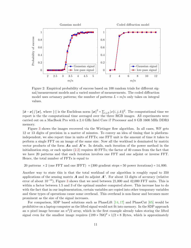
power method outlined in Algorithm 3 from Appendix B. In the iteration (2.2), we use the parametervalue µτ = min(1 − exp(−τ/τ0),0.2) where τ0 ≈ 330. We stop after 2,500 iterations, and report theempirical probability of success for the two different signal models. The empirical probability ofsucccess is an average over 100 trials, where in each instance, we generate new random samplingvectors according to the Gaussian or CDP models. We declare a trial successful if the relative errorof the reconstruction dist(x,x)/ ∥x∥ falls below 10−5.

Figure 2 shows that around 4.5n Gaussian phaseless measurements suffice for exact recoverywith high probability via the Wirtinger flow algorithm. We also see that about six octanary patternsare sufficient.

4.3 Performance on natural images

We move on to testing the Wirtinger flow algorithm on various images of different sizes; these arephotographs of the Naqsh-e Jahan Square in the central Iranian city of Esfahan, the Stanford mainquad, and the Milky Way galaxy. Since each photograph is in color, we run the WF algorithm oneach of the three RGB images that make up the photograph. Color images are viewed as n1×n2×3arrays, where the first two indices encode the pixel location, and the last the color band.

We generate L = 20 random octanary patterns and gather the coded diffraction patterns foreach color band using these 20 samples. As before, we run 50 iterations of the power method asthe initialization step. The updates use the sequence µτ = min(1 − exp(−τ/τ0),0.4) where τ0 ≈ 330as before. In all cases we run 300 iterations and record the relative recovery error as well as therunning time. If x and x are the original and recovered images, the relative error is equal to

10

2 2.5 3 3.5 4 4.5 5

0

0.2

0.4

0.6

0.8

1

m/n

Pro

bab

ilit

yof

succ

ess

Gaussian model

Gaussian signallow-pass signal

2 4 6 8 10 12

0

0.2

0.4

0.6

0.8

1

m/n

Coded diffraction model

Gaussian signallow-pass signal

Figure 2: Empirical probability of success based on 100 random trials for different sig-nal/measurement models and a varied number of measurements. The coded diffractionmodel uses octanary patterns; the number of patterns L =m/n only takes on integralvalues.

∥x −x∥ / ∥x∥, where ∥⋅∥ is the Euclidean norm ∥x∥2= ∑i,j,k ∣x(i, j, k)∣

2. The computational time wereport is the the computational time averaged over the three RGB images. All experiments werecarried out on a MacBook Pro with a 2.4 GHz Intel Core i7 Processor and 8 GB 1600 MHz DDR3memory.

Figure 3 shows the images recovered via the Wirtinger flow algorithm. In all cases, WF gets12 or 13 digits of precision in a matter of minutes. To convey an idea of timing that is platform-independent, we also report time in units of FFTs; one FFT unit is the amount of time it takes toperform a single FFT on an image of the same size. Now all the workload is dominated by matrixvector products of the form Az and A∗v. In details, each iteration of the power method in theinitialization step, or each update (2.2) requires 40 FFTs; the factor of 40 comes from the fact thatwe have 20 patterns and that each iteration involves one FFT and one adjoint or inverse FFT.Hence, the total number of FFTs is equal to

20 patterns × 2 (one FFT and one IFFT) × (300 gradient steps + 50 power iterations) = 14,000.

Another way to state this is that the total workload of our algorithm is roughly equal to 350applications of the sensing matrix A and its adjoint A∗. For about 13 digits of accuracy (relativeerror of about 10−13), Figure 3 shows that we need between 21,000 and 42,000 FFT units. This iswithin a factor between 1.5 and 3 of the optimal number computed above. This increase has to dowith the fact that in our implementation, certain variables are copied into other temporary variablesand these types of operations cause some overhead. This overhead is non-linear and becomes moreprominent as the size of the signal increases.

For comparison, SDP based solutions such as PhaseLift [14, 17] and PhaseCut [65] would beprohibitive on a laptop computer as the lifted signal would not fit into memory. In the SDP approachan n pixel image become an n2/2 array, which in the first example already takes storing the liftedsignal even for the smallest image requires (189 × 768)2 × 1/2 × 8 Bytes, which is approximately

11

85 GB of space. (For the image of the Milky Way, storage would be about 17 TB.) These largememory requirements prevent the application of full-blown SDP solvers on desktop computers.

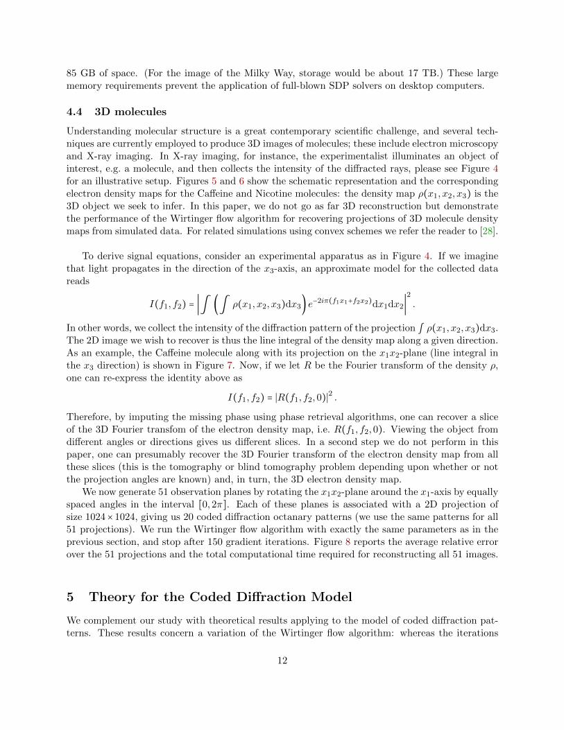
4.4 3D molecules

Understanding molecular structure is a great contemporary scientific challenge, and several tech-niques are currently employed to produce 3D images of molecules; these include electron microscopyand X-ray imaging. In X-ray imaging, for instance, the experimentalist illuminates an object ofinterest, e.g. a molecule, and then collects the intensity of the diffracted rays, please see Figure 4for an illustrative setup. Figures 5 and 6 show the schematic representation and the correspondingelectron density maps for the Caffeine and Nicotine molecules: the density map ρ(x1, x2, x3) is the3D object we seek to infer. In this paper, we do not go as far 3D reconstruction but demonstratethe performance of the Wirtinger flow algorithm for recovering projections of 3D molecule densitymaps from simulated data. For related simulations using convex schemes we refer the reader to [28].

To derive signal equations, consider an experimental apparatus as in Figure 4. If we imaginethat light propagates in the direction of the x3-axis, an approximate model for the collected datareads

I(f1, f2) = ∣∫ (∫ ρ(x1, x2, x3)dx3) e−2iπ(f1x1+f2x2)dx1dx2∣

2

.

In other words, we collect the intensity of the diffraction pattern of the projection ∫ ρ(x1, x2, x3)dx3.The 2D image we wish to recover is thus the line integral of the density map along a given direction.As an example, the Caffeine molecule along with its projection on the x1x2-plane (line integral inthe x3 direction) is shown in Figure 7. Now, if we let R be the Fourier transform of the density ρ,one can re-express the identity above as

I(f1, f2) = ∣R(f1, f2,0)∣2 .

Therefore, by imputing the missing phase using phase retrieval algorithms, one can recover a sliceof the 3D Fourier transfom of the electron density map, i.e. R(f1, f2,0). Viewing the object fromdifferent angles or directions gives us different slices. In a second step we do not perform in thispaper, one can presumably recover the 3D Fourier transform of the electron density map from allthese slices (this is the tomography or blind tomography problem depending upon whether or notthe projection angles are known) and, in turn, the 3D electron density map.

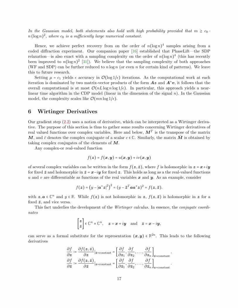
We now generate 51 observation planes by rotating the x1x2-plane around the x1-axis by equallyspaced angles in the interval [0,2π]. Each of these planes is associated with a 2D projection ofsize 1024× 1024, giving us 20 coded diffraction octanary patterns (we use the same patterns for all51 projections). We run the Wirtinger flow algorithm with exactly the same parameters as in theprevious section, and stop after 150 gradient iterations. Figure 8 reports the average relative errorover the 51 projections and the total computational time required for reconstructing all 51 images.

5 Theory for the Coded Diffraction Model

We complement our study with theoretical results applying to the model of coded diffraction pat-terns. These results concern a variation of the Wirtinger flow algorithm: whereas the iterations

12

(a) Naqsh-e Jahan Square, Esfahan. Image size is 189 × 768 pixels; timing is 61.4sec or about 21,200 FFT units. The relative error is 6.2 × 10−16.

(b) Stanford main quad. Image size is 320 × 1280 pixels; timing is 181.8120 sec orabout 20,700 FFT units. The relative error is 3.5 × 10−14.

(c) Milky way Galaxy. Image size is 1080 × 1920 pixels; timing is 1318.1 sec or41,900 FFT units. The relative error is 9.3 × 10−16.

Figure 3: Performance of the WF algorithm on three scenic images. Image size,computational time in seconds and in units of FFTs are reported, as well as the relativeerror after 300 WF iterations.

13

source

molecule

diffraction patterns

Figure 4: An illustrative setup of diffraction patterns.

(a) Schematic representation (b) Electron density map

Figure 5: Schematic representation and electron density map of the Caffeine molecule.

(a) Schematic representation (b) Electron density map

Figure 6: Schematic representation and electron density map of the Nicotine molecule.

14

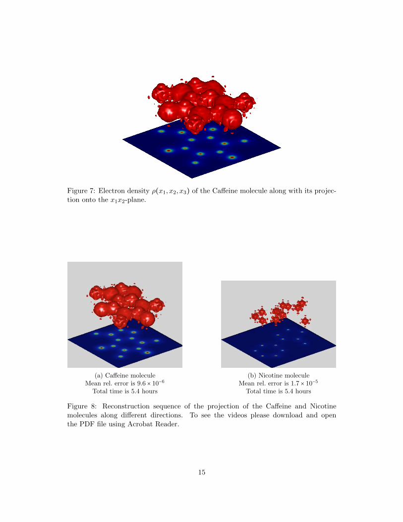
Figure 7: Electron density ρ(x1, x2, x3) of the Caffeine molecule along with its projec-tion onto the x1x2-plane.

(a) Caffeine moleculeMean rel. error is 9.6 × 10−6

Total time is 5.4 hours

(b) Nicotine moleculeMean rel. error is 1.7 × 10−5

Total time is 5.4 hours

Figure 8: Reconstruction sequence of the projection of the Caffeine and Nicotinemolecules along different directions. To see the videos please download and openthe PDF file using Acrobat Reader.

15

are exactly the same as (2.2), the initialization applies an iterative scheme which uses fresh setsof sample at each iteration. This is described in Algorithm 2. In the CDP model, the partition-ing assigns to the same group all the observations and sampling vectors corresponding to a givenrealization of the random code. This is equivalent to partitioning the random patterns into B + 1groups. As a result, sampling vectors in distinct groups are stochastically independent.

Algorithm 2 Initialization via resampled Wirtinger Flow

Input: Observations {yr} ∈ Rm and number of blocks B.Partition the observations and sampling vectors {yr}

mr=1 and {ar}

mr=1 into B + 1 groups of size

m′ = ⌊m/(B + 1)⌋. For each group b = 0,1, . . . ,B, set

f(z; b) =1

2m′

m′

∑r=1

(y(b)r − ∣⟨a(b)r ,z⟩∣

2)

2

,

where {a(b)r } are those sampling vectors belonging to the bth group (and likewise for {y

(b)r }).

Initialize u0 to be eigenvector corresponding to the largest eigenvalue of

Y =1

m′

m′

∑r=1

y(0)r a(0)r a(0)

r

∗

normalized as in Algorithm (1).Loop:for b = 0 to B − 1 do

ub+1 = ub −µ

∥u0∥2∇f(ub; b)

end forOutput: z0 = uB.

Theorem 5.1 Let x be an arbitrary vector in Cn and assume we collect L admissible coded diffrac-tion patterns with L ≥ c0 ⋅ (logn)4, where c0 is a sufficiently large numerical constant. Then theinitial solution z0 of Algorithm 25 obeys

dist(z0,x) ≤1

8√n

∥x∥ (5.1)

with probability at least 1 − (4L + 2)/n3. Further, take a constant learning parameter sequence,µτ = µ for all τ = 1,2, . . . and assume µ ≤ c1 for some fixed numerical constant c1. Then there is anevent of probability at least 1− (2L+ 1)/n3 − 1/n2, such that on this event, starting from any initialsolution z0 obeying (5.1), we have

dist(zτ ,x) ≤1

8√n

(1 −µ

3)τ/2

⋅ ∥x∥ . (5.2)

5We choose the number of partitions B in Algorithm 2 to obey B ≥ c1 logn for c1 a sufficiently large numericalconstant.

16

In the Gaussian model, both statements also hold with high probability provided that m ≥ c0 ⋅

n (logn)2, where c0 is a sufficiently large numerical constant.

Hence, we achieve perfect recovery from on the order of n(logn)4 samples arising from acoded diffraction experiment. Our companion paper [16] established that PhaseLift—the SDPrelaxation—is also exact with a sampling complexity on the order of n(logn)4 (this has recentlybeen improved to n(logn)2 [31]). We believe that the sampling complexity of both approaches(WF and SDP) can be further reduced to n logn (or even n for certain kind of patterns). We leavethis to future research.

Setting µ = c1 yields ε accuracy in O(log 1/ε) iterations. As the computational work at eachiteration is dominated by two matrix-vector products of the form Az and A∗v, it follows that theoverall computational is at most O(nL logn log 1/ε). In particular, this approach yields a near-linear time algorithm in the CDP model (linear in the dimension of the signal n). In the Gaussianmodel, the complexity scales like O(mn log 1/ε).

6 Wirtinger Derivatives

Our gradient step (2.2) uses a notion of derivative, which can be interpreted as a Wirtinger deriva-tive. The purpose of this section is thus to gather some results concerning Wirtinger derivatives ofreal valued functions over complex variables. Here and below, MT is the transpose of the matrixM , and c denotes the complex conjugate of a scalar c ∈ C. Similarly, the matrix M is obtained bytaking complex conjugates of the elements of M .

Any complex-or real-valued function

f(z) = f(x,y) = u(x,y) + iv(x,y)

of several complex variables can be written in the form f(z, z), where f is holomorphic in z = x+iyfor fixed z and holomorphic in z = x−iy for fixed z. This holds as long as a the real-valued functionsu and v are differentiable as functions of the real variables x and y. As an example, consider

f(z) = (y − ∣a∗z∣2)

2= (y − zTaa∗z)2

= f(z, z).

with z,a ∈ Cn and y ∈ R. While f(z) is not holomorphic in z, f(z, z) is holomorphic in z for afixed z, and vice versa.

This fact underlies the development of the Wirtinger calculus. In essence, the conjugate coordi-nates

[zz] ∈ Cn ×Cn, z = x + iy and z = x − iy,

can serve as a formal substitute for the representation (x,y) ∈ R2n. This leads to the followingderivatives

∂f

∂z∶=∂f(z, z)

∂z∣z=constant = [

∂f

∂z1,∂f

∂z2, . . . ,

∂f

∂zn]z=constant

,

∂f

∂z∶=∂f(z, z)

∂z∣z=constant = [

∂f

∂z1,∂f

∂z2, . . . ,

∂f

∂zn]z=constant

.

17

Our definitions follow standard notation from multivariate calculus so that derivatives are rowvectors and gradients are column vectors. In this new coordinate system the complex gradient isgiven by

∇cf = [∂f

∂z,∂f

∂z]

∗.

Similarly, we define

Hzz ∶=∂

∂z(∂f

∂z)

∗, Hzz ∶=

∂

∂z(∂f

∂z)

∗, Hzz ∶=

∂

∂z(∂f

∂z)

∗, Hzz ∶=

∂

∂z(∂f

∂z)

∗.

In this coordinate system the complex Hessian is given by

∇2f ∶= [

Hzz Hzz

Hzz Hzz] .

Given vectors z and ∆z ∈ Cn, we have defined the gradient and Hessian in a manner such thatTaylor’s approximation takes the form

f(z +∆z) ≈ f(z) + (∇cf(z))∗⎡⎢⎢⎢⎢⎣

∆z

∆z

⎤⎥⎥⎥⎥⎦

+1

2

⎡⎢⎢⎢⎢⎣

∆z

∆z

⎤⎥⎥⎥⎥⎦

∗

∇2f(z)

⎡⎢⎢⎢⎢⎣

∆z

∆z

⎤⎥⎥⎥⎥⎦

.

If we were to run gradient descent in this new coordinate system, the iterates would be

[zτ+1

zτ+1] = [

zτzτ

] − µ [(∂f/∂z)

∗∣z=zτ

(∂f/∂z)∗∣z=zτ

] (6.1)

Note that when f is a real-valued function (as in this paper) we have

∂f

∂z=∂f

∂z.

Therefore, the second set of updates in (6.1) is just the conjugate of the first. Thus, it is sufficientto keep track of the first update, namely,

zτ+1 = zτ − µ (∂f/∂z)∗ .

For real valued functions of complex variables, setting

∇f(z) = (∂f

∂z)

∗

gives the gradient update

zτ+1 = zτ − µ∇f(zτ).

The reader may wonder why we choose to work with conjugate coordinates as there are alterna-tives: in particular, we could view the complex variable z = x + iy ∈ Cn as a vector in R2n and justrun gradient descent in the x,y coordinate system. The main reason why conjugate coordinates areparticularly attractive is that expressions for derivatives become significantly simpler and resemblethose we obtain in the real case, where f ∶ Rn → R is a function of real variables.

18

7 Proofs

7.1 Preliminaries

We first note that in the CDP model with admissible CDPs ∥ar∥ ≤√

6n for all r = 1,2, . . . ,m,as in our CDP model ∣d∣ ≤

√3 <

√6. In the Gaussian model the measurements vectors also obey

∥ar∥ ≤√

6n for all r = 1,2, . . . ,m with probability at least 1 −me−1.5n. Throughout the proofs, weassume we are on this event without explicitly mentioning it each time.

Before we begin with the proofs we should mention that we will prove our result using theupdate

zτ+1 = zτ −µ

∥x∥2∇f(zτ), (7.1)

in lieu of the WF update

zτ+1 = zτ −µWF

∥z0∥2∇f(zτ). (7.2)

Since ∣∥z0∥2− ∥x∥

2∣ ≤ 1

64 ∥x∥2 holds with high probability as proven in Section 7.8, we have

∥z0∥2≥

63

64∥x∥

2. (7.3)

Therefore, the results for the update (7.1) automatically carry over to the WF update with a simplerescaling of the upper bound on the learning parameter. More precisely, if we prove that the update(7.1) converges to a global optimum as long as µ ≤ µ0, then the convergence of the WF update to aglobal optimum is guaranteed as long as µWF ≤ 63

64µ0. Also, the update in (7.1) is invariant to theEuclidean norm of x. Therefore, without loss of generality we will assume throughout the proofsthat ∥x∥ = 1.

We remind the reader that throughout x is a solution to our quadratic equations, i.e. obeysy = ∣Ax∣2 and that the sampling vectors are independent from x. Define

P ∶= {xeiφ ∶ φ ∈ [0,2π]}.

to be the set of all vectors that differ from the planted solution x only by a global phase factor.We also introduce the set of all points that are close to P ,

E(ε) ∶= {z ∈ Cn ∶ dist(z, P ) ≤ ε}, (7.4)

Finally for any vector z ∈ Cn we define the phase φ(z) as

φ(z) ∶= arg minφ∈[0,2π]

∥z − eiφx∥ ,

so that

dist(z,x) = ∥z − eiφ(z)x∥ .

19

7.2 Formulas for the complex gradient and Hessian

We gather some useful gradient and Hessian calculations that will be used repeatedly. Startingwith

f(z) =1

2m

m

∑r=1

(yr − zT (ara∗r)z)

2=

1

2m

m

∑r=1

(yr − zT (ara∗r)T z)

2,

we establish

(∂

∂zf(z))

T

=1

m

m

∑r=1

(zT (ara∗r)T z − yr) (ara

∗r)T z.

This gives

∇f(z) = (∂

∂zf(z))

∗=

1

m

m

∑r=1

(zT (ara∗r)z − yr) (ara

∗r)z.

For the second derivative, we write

Hzz =∂

∂z(∂

∂zf(z))

∗=

1

m

m

∑r=1

(2∣a∗rz∣2− yr)ara

∗r

and

Hzz =∂

∂z(∂

∂zf(z))

∗=

1

m

m

∑r=1

(a∗rz)2ara

Tr .

Therefore,

∇2f(z) =

1

m

m

∑r=1

[(2 ∣a∗rz∣

2− yr)ara

∗r (a∗rz)

2araTr

(a∗rz)2ara

∗r (2 ∣a∗rz∣

2− yr)ara

Tr

] .

7.3 Expectation and concentration

This section gathers some useful intermediate results whose proofs are deferred to Appendix A. Thefirst two lemmas establish the expectation of the Hessian, gradient and a related random variablein both the Gaussian and admissible CDP models.6

Lemma 7.1 Recall that x is a solution obeying ∥x∥ = 1, which is independent from the samplingvectors. Furthermore, assume the sampling vectors ar are distributed according to either the Gaus-sian or admissible CDP model. Then

E[∇2f(x)] = I2n +

3

2[xx] [x∗,xT ] −

1

2[x−x

] [x∗,−xT ].

Lemma 7.2 In the setup of Lemma 7.1, let z ∈ Cn be a fixed vector independent of the samplingvectors. We have

E[∇f(z)] = (I −xx∗)z + 2 (∥z∥2− 1)z.

The next lemma gathers some useful identities in the Gaussian model.

6In the CDP model the expectation is with respect to the random modulation pattern.

20

Lemma 7.3 Assume u,v ∈ Cn are fixed vectors obeying ∥u∥ = ∥v∥ = 1 which are independent ofthe sampling vectors. Furthermore, assume the measurement vectors ar are distributed accordingto the Gaussian model. Then

E [ (Re(u∗ara∗rv))

2] =

1

2+

3

2(Re(u∗v))2

−1

2(Im(u∗v))2 (7.5)

E [Re(u∗ara∗rv) ∣a

∗rv∣

2] =2 Re(u∗v) (7.6)

E [ ∣a∗rv∣2k

] =k!. (7.7)

The next lemma establishes the concentration of the Hessian around its mean for both theGaussian and the CDP model.

Lemma 7.4 In the setup of Lemma 7.1, assume the vectors ar are distributed according to eitherthe Gaussian or admissible CDP model with a sufficiently large number of measurements. Thismeans that the number of samples obeys m ≥ c(δ) ⋅ n logn in the Gaussian model and the numberof patterns obeys L ≥ c(δ) ⋅ log3 n in the CDP model. Then

∥∇2f(x) − E[∇

2f(x)]∥ ≤ δ, (7.8)

holds with probability at least 1 − 10e−γn − 8/n2 and 1 − (2L + 1)/n3 for the Gaussian and CDPmodels, respectively.

We will also make use of the two results below, which are corollaries of the three lemmas above.These corollaries are also proven in Appendix A.

Corollary 7.5 Suppose ∥∇2f(x) − E[∇2f(x)]∥ ≤ δ. Then for all h ∈ Cn obeying ∥h∥ = 1, we have

1

m

m

∑r=1

Re (h∗ara∗rx)

2=

1

4

m

∑r=1

[hh]

∗

∇2f(x) [

hh] ≤ (

1

2∥h∥

2+

3

2Re(x∗h)

2−

1

2Im(x∗h)

2) +

δ

2.

In the other direction,

1

m

m

∑r=1

Re (h∗ara∗rx)

2≥ (

1

2∥h∥

2+

3

2Re(x∗h)

2−

1

2Im(x∗h)

2) −

δ

2.

Corollary 7.6 Suppose ∥∇2f(x) − E[∇2f(x)]∥ ≤ δ. Then for all h ∈ Cn obeying ∥h∥ = 1, we have

1

m

m

∑r=1

∣a∗rx∣2∣a∗rh∣

2= h∗ (

1

m

m

∑r=1

∣a∗rx∣2ara

∗r)h ≥ (1 − δ) ∥h∥

2+ ∣h∗x∣

2≥ (1 − δ) ∥h∥

2 ,

and

1

m

m

∑r=1

∣a∗rx∣2∣a∗rh∣

2= h∗ (

1

m

m

∑r=1

∣a∗rx∣2ara

∗r)h ≤ (1 + δ) ∥h∥

2+ ∣h∗x∣

2≤ (2 + δ) ∥h∥

2 .

The next lemma establishes the concentration of the gradient around its mean for both Gaussianand admissible CDP models.

21

Lemma 7.7 In the setup of Lemma 7.4, let z ∈ Cn be a fixed vector independent of the samplingvectors obeying dist(z,x) ≤ 1

2 . Then

∥∇f(z) − E[∇f(z)]∥ ≤ δ ⋅ dist(z,x).

holds with probability at least 1− 20e−γm − 4m/n4 in the Gaussian model and 1− (4L+ 2)/n3 in theCDP model.

We finish with a result concerning the concentration of the sample covariance matrix.

Lemma 7.8 In the setup of Lemma 7.4,

∥In −m−1

m

∑r=1

ara∗r∥ ≤ δ,

holds with probability at least 1−2e−γm for the Gaussian model and 1−1/n2 in the CDP model. Onthis event,

(1 − δ) ∥h∥2≤

1

m

m

∑r=1

∣a∗rh∣2≤ (1 + δ) ∥h∥

2 for all h ∈ Cn. (7.9)

7.4 General convergence analysis

We will assume that the function f satisfies a regularity condition on E(ε), which essentially statesthat the gradient of the function is well behaved. We remind the reader that E(ε), as defined in(7.4), is the set of points that are close to the path of global minimizers.

Condition 7.9 (Regularity Condition) We say that the function f satisfies the regularity con-dition or RC(α,β, ε) if for all vectors z ∈ E(ε) we have

Re (⟨∇f(z),z −xeiφ(z)⟩) ≥1

αdist2

(z,x) +1

β∥∇f(z)∥2 . (7.10)

In the lemma below we show that as long as the regularity condition holds on E(ε) thenWirtinger Flow starting from an initial solution in E(ε) converges to a global optimizer at ageometric rate. Subsequent sections shall establish that this property holds.

Lemma 7.10 Assume that f obeys RC(α,β, ε) for all z ∈ E(ε). Furthermore, suppose z0 ∈ E, andassume 0 < µ ≤ 2/β. Consider the following update

zτ+1 = zτ − µ∇f(zτ).

Then for all τ we have zτ ∈ E(ε) and

dist2(zτ ,x) ≤ (1 −

2µ

α)τ

dist2(z0,x).

22

We note that for αβ < 4, (7.10) holds with the direction of the inequality reversed.7 Thus, ifRC(α,β, ε) holds, α and β must obey αβ ≥ 4. As a result, under the stated assumptions of Lemma7.10 above, the factor 1 − 2µ/α ≥ 1 − 4/(αβ) is non-negative.Proof The proof follows a structure similar to related results in the convex optimization literaturee.g. [53, Theorem 2.1.15]. However, unlike these classical results where the goal is often to proveconvergence to a unique global optimum, the objective function f does not have a unique globaloptimum. Indeed, in our problem, if x is solution, then eiφx is also solution. Hence, propermodification is required to prove convergence results.

We prove that if z ∈ E(ε) then for all 0 < µ ≤ 2/β

z+ = z − µ∇f(z)

obeys

dist2(z+,x) ≤ (1 −

2µ

α)dist2

(z,x). (7.11)

Therefore, if z ∈ E(ε) then we also have z+ ∈ E(ε). The lemma follows by inductively applying(7.11). Now simple algebraic manipulations together with the regularity condition (7.10) give

∥z+ −xeiφ(z)∥2= ∥z −xeiφ(z) − µ∇f(z)∥

2

= ∥z −xeiφ(z)∥2− 2µRe (⟨∇f(z), (z −xeiφ(z)) ⟩) + µ2

∥∇f(z)∥2

≤ ∥z −xeiφ(z)∥2− 2µ(

1

α∥z −xeiφ(z)∥

2+

1

β∥∇f(z)∥2

) + µ2∥∇f(z)∥2

=(1 −2µ

α)∥z −xeiφ(z)∥

2+ µ(µ −

2

β) ∥∇f(z)∥2

≤(1 −2µ

α)∥z −xeiφ(z)∥

2,

where the last line follows from µ ≤ 2/β. The definition of φ(z+) gives

∥z+ −xeiφ(z+)∥2≤ ∥z+ −xeiφ(z)∥

2,

which concludes the proof.

7.5 Proof of the regularity condition

For any z ∈ E(ε), we need to show that

Re (⟨∇f(z),z −xeiφ(z)⟩) ≥1

αdist2

(z,x) +1

β∥∇f(z)∥2 . (7.12)

We prove this with δ = 0.01 by establishing that our gradient satisfies the local smoothness andlocal curvature conditions defined below. Combining both these two properties gives (7.12).

7One can see this by applying Cauchy-Schwarz and calculating the determinant of the resulting quadratic form.

23

Condition 7.11 (Local Curvature Condition) We say that the function f satisfies the localcurvature condition or LCC(α, ε, δ) if for all vectors z ∈ E(ε),

Re (⟨∇f(z),z −xeiφ(z)⟩) ≥ (1

α+

(1 − δ)

4)dist2

(z,x) +1

10m

m

∑r=1

∣a∗r(z − eiφ(z)x)∣

4. (7.13)

This condition essentially states that the function curves sufficiently upwards (along most direc-tions) near the curve of global optimizers.

Condition 7.12 (Local Smoothness Condition) We say that the function f satisfies the localsmoothness condition or LSC(β, ε, δ) if for all vectors z ∈ E(ε) we have

∥∇f(z)∥2≤ β (

(1 − δ)

4dist2

(z,x) +1

10m

m

∑r=1

∣a∗r(z − eiφ(z)x)∣

4) . (7.14)

This condition essentially states that the gradient of the function is well behaved (the function doesnot vary too much) near the curve of global optimizers.

7.6 Proof of the local curvature condition

For any z ∈ E(ε), we want to prove the local curvature condition (7.13). Recall that

∇f(z) =1

m

m

∑r=1

(∣⟨ar,z⟩∣2− yr) (ara

∗r)z,

and define h ∶= e−iφ(z)z −x. To establish (7.13) it suffices to prove that

1

m

m

∑r=1

(2 Re(h∗ara∗rx)

2+ 3 Re(h∗ara

∗rx)∣a∗rh∣

2+ ∣a∗rh∣

4) − (1

10m

m

∑r=1

∣a∗rh∣4)

≥ (1

α+

(1 − δ)

4)∥h∥

2 , (7.15)

holds for all h satisfying Im(h∗x) = 0, ∥h∥2 ≤ ε. Equivalently, we only need to prove that for all hsatisfying Im(h∗x) = 0, ∥h∥2 = 1 and for all s with 0 ≤ s ≤ ε,

1

m

m

∑r=1

(2 Re(h∗ara∗rx)

2+ 3sRe(h∗ara

∗rx)∣a∗rh∣

2+

9

10s2

∣a∗rh∣4) ≥

1

α+

(1 − δ)

4. (7.16)

By Corollary 7.5, with high probability,

1

m

m

∑r=1

Re(h∗ara∗rx)

2≤

1 + δ

2+

3

2Re(x∗h)

2,

holds for all h obeying ∥h∥ = 1. Therefore, to establish the local curvature condition (7.13) itsuffices to show that

1

m

m

∑r=1

(5

2Re(h∗ara

∗rx)

2+ 3sRe(h∗ara

∗rx)∣a∗rh∣

2+

9

10s2

∣a∗rh∣4) ≥ (

1

α+

1

2)+

3

4Re(x∗h)

2. (7.17)

24

We will establish (7.17) for different measurement models and different values of ε. Below, it shallbe convenient to use the shorthand

Yr(h, s) ∶=5

2Re(h∗ara

∗rx)

2+ 3sRe(h∗ara

∗rx)∣a∗rh∣

2+

9

10s2

∣a∗rh∣4,

⟨Yr(h, s)⟩ ∶=1

m

m

∑r=1

Yr(h, s).

7.6.1 Proof of (7.17) with ε = 1/8√n in the Gaussian and CDP models

Set ε = 1/8√n. We show that with high probability, (7.17) holds for all h satisfying Im(h∗x) = 0,

∥h∥2 = 1, 0 ≤ s ≤ ε, δ ≤ 0.01, and α ≥ 30. First, note that by Cauchy-Schwarz inequality,

⟨Yr(h, s)⟩ ≥5

2m

m

∑r=1

Re(h∗ara∗rx)

2−

3s

m

¿ÁÁÀ

m

∑r=1

Re(h∗ara∗rx)2

¿ÁÁÀ

m

∑r=1

∣a∗rh∣4 +9

10

s2

m

m

∑r=1

∣a∗rh∣4

=⎛

⎝

¿ÁÁÀ 5

2m

m

∑r=1

Re(h∗ara∗rx)2 − s

¿ÁÁÀ 9

10m

m

∑r=1

∣a∗rh∣4⎞

⎠

2

≥5

4m

m

∑r=1

Re(h∗ara∗rx)

2−

9s2

10m

m

∑r=1

∣a∗rh∣4. (7.18)

The last inequality follows from (a − b)2 ≥ a2

2 − b2. By Corollary 7.5,

1

m

m

∑r=1

Re(h∗ara∗rx)

2≥

1 − δ

2+

3

2Re(x∗h)

2 (7.19)

holds with high probability for all h obeying ∥h∥ = 1. Furthermore, by applying Lemma 7.8,

1

m

m

∑r=1

∣a∗rh∣4≤ (max

r∥ar∥

2)(

1

m

m

∑r=1

∣a∗rh∣2) ≤ 6(1 + δ)n (7.20)

holds with high probability. Plugging (7.19) and (7.20) in (7.18) yields

⟨Yr(h, s)⟩ ≥15

8Re(x∗h)

2+

5

8(1 − δ) −

27

5s2

(1 + δ)n.

(7.17) follows by using α ≥ 30, ε = 18√n

and δ = 0.01.

7.6.2 Proof of (7.17) with ε = 1/8 in the Gaussian model

Set ε = 1/8. We show that with high probability, (7.17) holds for all h satisfying Im(h∗x) = 0,∥h∥2 = 1, 0 ≤ s ≤ ε, δ ≤ 2, and α ≥ 8. To this end, we first state a result about the tail of a sumof i.i.d. random variables. Below, Φ is the cumulative distribution function of a standard normalvariable.

Lemma 7.13 ( [11]) Suppose X1,X2, . . . ,Xm are i.i.d. real-valued random variables obeying Xr ≤

b for some nonrandom b > 0, EXr = 0, and EX2r = v

2. Setting σ2 =mmax(b2, v2),

P(X1 + . . . +Xm ≥ y) ≤ min(exp(−y2

2σ2) , c0 (1 −Φ(y/σ)))

where one can take c0 = 25.

25

To establish (7.17) we first prove it for a fixed h, and then use a covering argument. Observe that

Yr ∶= Yr(h, s) =⎛

⎝

√5

2Re(h∗ara

∗rx) +

√9

10s ∣a∗rh∣

2⎞

⎠

2

.

By Lemma 7.3,

E[Re(h∗ara∗rx)

2] =

1

2+

3

2(Re(x∗h))

2 and E[Re(h∗ara∗rx)∣a∗rh∣

2] = 2 Re(u∗v),

compare (7.5) and (7.6). Therefore, using s ≤ 18 ,

µr = EYr =5

4(1 + 3 Re(x∗h)

2) + 6sRe(x∗h) +

27

10s2

< 6.

Now define Xr = µr −Yr. First, since Yr ≥ 0, Xr ≤ µr < 6. Second, we bound EX2r using Lemma 7.3

and Holder’s inequality with s ≤ 1/8:

EX2r ≤ EY 2

r =25

4E[Re(h∗ara

∗rx)

4] +

81

100s4 E[∣a∗rh∣

8] +

27

2s2 E[Re(h∗ara

∗rx)

2∣a∗rh∣

4]

+ 15sE[Re(h∗ara∗rx)

3∣a∗rh∣

2] +

27

5s3 E[Re(h∗ara

∗rx) ∣a∗rh∣

6]

≤25

4

√

E[∣a∗rh∣8]E[∣a∗rx∣

8] +

81

100s4 E[∣a∗rh∣

8] +

27

2s2

√

E[∣a∗rh∣12]E[∣a∗rx∣

4]

+ 15s√

E[∣a∗rh∣10]E[∣a∗rx∣

6] +

27

5s3

√

E[∣a∗rh∣14]E[∣a∗rx∣

2]

< 20s4+ 543s3

+ 513s2+ 403s + 150

< 210.

We have all the elements to apply Lemma 7.13 with σ2 =mmax(92,210) = 210m and y =m/4:

P(mµ −m

∑r=1

Yr ≥m

4) ≤ e−3γm

with γ = 1/1260. Therefore, with probability at least 1 − e−3γm, we have

⟨Yr(h, s)⟩ ≥5

4(1 + 3 Re(x∗h)

2) + 6sRe(x∗h) + 2.7s2

−1

4

≥3

4+

1

16+

3

4Re(x∗h)

2+ 3 (Re(x∗h) + s)

2+ (

3

16−

3

10s2

)

≥3

4+

1

16+

3

4Re(x∗h)

2. (7.21)

provided that s ≤ 1/8. The inequality above holds for a fixed vector h and a fixed value s. To prove(7.17) for all s ≤ 1/8 and all h ∈ Cn with ∥h∥ = 1, define

pr(h, s) ∶=

√5

2Re(h∗ara

∗rx) +

√9

10s ∣a∗rh∣

2.

26

Using the fact that maxr ∥ar∥ ≤√

6n and s ≤ 1/8, we have ∣pr(h, s)∣ ≤ 2 ∣a∗rh∣ ∣a∗rx∣ + s ∣a∗rh∣2≤ 13n.

Moreover, for any u,v ∈ Cn obeying ∥u∥ = ∥v∥ = 1,

∣pr(u, s) − pr(v, s)∣ ≤RRRRRRRRRRR

√5

2Re ((u − v)∗ara

∗rx)

RRRRRRRRRRR

+

√9

10s (∣a∗ru∣ + ∣a∗rv∣) ∣a

∗r(u − v)∣ ≤

27

2n ∥u − v∥ .

Introduce

q(h, s) ∶=1

m

m

∑r=1

pr(h, s)2−

3

4Re(x∗h)

2= ⟨Yr(h, s)⟩ −

3

4Re(x∗h)

2.

For any u,v ∈ Cn obeying ∥u∥ = ∥v∥ = 1,

∣q(u, s) − q(v, s)∣ = ∣1

m

m

∑r=1

(pr(u, s) − pr(v, s))(pr(u, s) + pr(v, s)) −3

4Re(x∗(u − v))Re(x∗(u + v))∣

≤27n

2× 2 × 13n ∥u − v∥ +

3

2∥u − v∥

= (351n2+

3

2) ∥u − v∥ . (7.22)

Therefore, for any u,v ∈ Cn obeying ∥u∥ = ∥v∥ = 1 and ∥u − v∥ ≤ η ∶= 16000n2 , we have

q(v, s) ≥ q(u, s) −1

16. (7.23)

Let Nη be an η-net for the unit sphere of Cn with cardinality obeying ∣Nη ∣ ≤ (1 + 2η )

2n. Applying

(7.21) together with the union bound we conclude that for all u ∈ Nη and a fixed s

P(q(u, s) ≥3

4+

1

16) ≥ 1 − ∣Nη ∣e

−3γm

≥ 1 − (1 + 12000n2)ne−3γm

≥ 1 − e−2γm. (7.24)

The last line follows by choosing m such that m ≥ c ⋅n logn, where c is a sufficiently large constant.Now for any h on the unit sphere of Cn, there exists a vector u ∈ Nη such that ∥h −u∥ ≤ η. Bycombining (7.23) and (7.24), q(h, s) ≥ 3

4 holds with probability at least 1−e−2γm for all h with unitEuclidean norm and for a fixed s. Applying a similar covering number argument over s ≤ 1/8 wecan further conclude that for all h and s

q(h, s) ≥3

4+

1

16−

1

16>

5

8⇒ ⟨Yr(h, s)⟩ ≥ (

1

8+

1

2) +

3

4Re(x∗h)

2,

holds with probability at least 1 − eγn as long as m ≥ c ⋅ n logn. This concludes the proof of (7.17)with α ≥ 8.

7.7 Proof of the local smoothness condition

For any z ∈ E(ε), we want to prove (7.14), which is equivalent to proving that for all u ∈ Cn obeying∥u∥ = 1, we have

∣(∇f(z))∗u∣2≤ β (

(1 − δ)

4dist2

(z,x) +1

10m

m

∑r=1

∣a∗r(z − eiφ(z)x)∣

4) .

27

Recall that

∇f(z) =1

m

m

∑r=1

(∣⟨ar,z⟩∣2− yr) (ara

∗r)z

and define

g(h,w, s) =1

m

m

∑r=1

(2 Re(h∗ara∗rx)Re(w∗ara

∗rx) + s∣a∗rh∣

2 Re(w∗ara∗rx)

+ 2sRe(h∗ara∗rx)Re(w∗ara

∗rh) + s2

∣a∗rh∣2 Re(w∗ara

∗rh)).

Define h ∶= e−φ(z)z −x and w ∶= e−iφ(z)u, to establish (7.14) it suffices to prove that

∣g(h,w,1)∣2 ≤ β (1 − δ

4∥h∥

2+

1

10m

m

∑r=1

∣a∗rh∣4) . (7.25)

holds for all h and w satisfying Im(h∗x) = 0, ∥h∥ ≤ ε and ∥w∥ = 1. Equivalently, we only need toprove for all h and w satisfying Im(h∗x) = 0, ∥h∥ = ∥w∥ = 1 and ∀s ∶ 0 ≤ s ≤ ε,

∣g(h,w, s)∣2 ≤ β (1 − δ

4+

s2

10m

m

∑r=1

∣a∗rh∣4) . (7.26)

Note that since (a + b + c)2 ≤ 3(a2 + b2 + c2)

∣g(h,w, s)∣2 ≤RRRRRRRRRRR

1

m

m

∑r=1

(2∣h∗ar ∣∣w∗ar ∣∣a

∗rx∣

2+ 3s∣h∗ar ∣

2∣a∗rx∣∣w∗ar ∣ + s

2∣a∗rh∣

3∣w∗ar ∣)

RRRRRRRRRRR

2

≤ 3RRRRRRRRRRR

2

m

m

∑r=1

∣h∗ar ∣∣w∗ar ∣∣a

∗rx∣

2RRRRRRRRRRR

2

+ 3RRRRRRRRRRR

3s

m

m

∑r=1

∣h∗ar ∣2∣a∗rx∣∣w∗ar ∣

RRRRRRRRRRR

2

+ 3RRRRRRRRRRR

s2

m

m

∑r=1

∣a∗rh∣3∣w∗ar ∣

RRRRRRRRRRR

2

∶= 3(I1 + I2 + I3). (7.27)

We now bound each of the terms on the right-hand side. For the first term we use Cauchy-Schwarzand Corollary 7.6, which give

I1 ≤ (1

m

m

∑r=1

∣a∗rx∣2∣a∗rw∣

2)(

1

m

m

∑r=1

∣a∗rx∣2∣a∗rh∣

2) ≤ (2 + δ)2. (7.28)

Similarly, for the second term, we have

I2 ≤ (1

m

m

∑r=1

∣a∗rh∣4)(

1

m

m

∑r=1

∣a∗rw∣2∣a∗rx∣

2) ≤

2 + δ

m

m

∑r=1

∣a∗rh∣4. (7.29)

Finally, for the third term we use the Cauchy-Schwarz inequality together with Lemma 7.8 (in-equality) (7.9) to derive

I3 ≤ (1

m

m

∑r=1

∣a∗rh∣3

maxr

∥ar∥)

2

≤ 6n(1

m

m

∑r=1

∣a∗rh∣3)

2

≤ 6n(1

m

m

∑r=1

∣a∗rh∣4)(

m

∑r=1

∣a∗rh∣2)

≤6n(1 + δ)

m

m

∑r=1

∣a∗rh∣4. (7.30)

28

We now plug these inequalities into (7.27) and get

∣g(h,w, s)∣2 ≤ 12(2 + δ)2+

27s2(2 + δ)

m

m

∑r=1

∣a∗rh∣4+

18s4n(1 + δ)

m

m

∑r=1

∣a∗rh∣4

≤ β (1 − δ

4+

s2

10m

m

∑r=1

∣a∗rh∣4) , (7.31)

which completes the proof of (7.26) and, in turn, establishes the local smoothness condition in(7.14). However, the last line of (7.31) holds as long as

β ≥ max(48(2 + δ)2

1 − δ,270(2 + δ) + 180ε2n(1 + δ)) . (7.32)

In our theorems we use two different values of ε = 18√n

and ε = 18 . Using δ ≤ 0.01 in (7.32) we

conclude that the local smoothness condition (7.31) holds as long as

β ≥ 550 for ε = 1/(8√n),

β ≥ 3n + 550 for ε = 1/8.

7.8 Wirtinger flow initialization

In this section, we prove that the WF initialization obeys (3.1) from Theorem 3.3. Recall that

Y ∶=1

m

m

∑r=1

∣a∗rx∣2ara

∗r .

and that Lemma 7.4 gives

∥Y − (xx∗ + ∥x∥2 I)∥ ≤ δ ∶= 0.001.

Let z0 be the eigenvector corresponding to the top eigenvalue λ0 of Y obeying ∥z0∥ = 1. It is easyto see that

∣λ0 − (∣z∗0x∣2+ 1)∣ = ∣z∗0Y z0 − z∗0(xx

∗+ I)z0∣ = ∣z∗0 (Y − (xx∗ + I)) z0∣ ≤ ∥Y − (xx∗ + I)∥ ≤ δ.

Therefore,∣z∗0x∣

2≥ λ0 − 1 − δ.

Also, since λ0 is the top eigenvalue of Y , and ∥x∥ = 1, we have

λ0 ≥ x∗Y x = x∗ (Y − (I +xx∗))x + 2 ≥ 2 − δ.

Combining the above two inequalities together, we have

∣z∗0x∣2≥ 1 − 2δ ⇒ dist2

(z0,x) ≤ 2 − 2√

1 − 2δ <1

256⇒ dist(z0,x) ≤

1

16.

Recall that z0 = (

√1m ∑

mr=1 ∣a

∗rx∣2) z0. By Lemma 7.8, equation (7.9), with high probability we

have

∣∥z0∥2− 1∣ = ∣

1

m

m

∑r=1

∣a∗rx∣2− 1∣ ≤

31

256⇒ ∣∥z0∥ − 1∣ ≤

1

16.

Therefore, we have

dist(z0,x) ≤ ∥z0 − z0∥ + dist(z0,x) = ∣∥z0∥ − 1∣ + dist(z0,x) ≤1

8.

29

7.9 Initialization via resampled Wirtinger Flow

In this section, we prove that that the output of Algorithm 2 obeys (5.1) from Theorem 5.1.Introduce

F (z) =1

2z∗(I −xx∗)z + (∥z∥2

− 1)2.

By Lemma 7.2, if z ∈ Cn is a vector independent from the measurements, then

E∇f(z; b) = ∇F (z).

We prove that F obeys a regularization condition in E(1/8), namely,

Re (⟨∇F (z),z −xeiφ(z)⟩) ≥1

α′dist2

(z,x) +1

β′∥∇F (z)∥2 . (7.33)

Lemma 7.7 implies that for a fixed vector z,

Re (⟨∇f(z; b),z −xeiφ(z)⟩) =Re (⟨∇F (z),z −xeiφ(z)⟩) +Re (⟨∇f(z; b) −∇F (z),z −xeiφ(z)⟩)

≥Re (⟨∇F (z),z −xeiφ(z)⟩) − ∥∇f(z; b) −∇F (z)∥dist(z,x)

≥Re (⟨∇F (z),z −xeiφ(z)⟩) − δdist(z,x)2

≥(1

α′− δ)dist(z,x)

2+

1

β′∥∇F (z)∥2 , (7.34)

holds with high probability. The last inequality follows from (7.33). Applying Lemma 7.7, we alsohave

∥∇F (z)∥2≥

1

2∥∇f(z; b)∥2

− ∥∇f(z; b) −∇F (z)∥2≥

1

2∥∇f(z; b)∥2

− δ2dist(z,x)2.

Plugging the latter into (7.34) yields

Re (⟨∇f(z; b),z −xeiφ(z)⟩) ≥ (1

α′−δ2

β′− δ)dist2

(z,x) +1

2β′∥∇f(z; b)∥

∶=1

αdist2

(z,x) +1

β∥∇f(z; b)∥ .

Therefore, using the general convergence analysis of gradient descent discussed in Section 7.4 weconclude that for all µ ≤ µ0 ∶= 2/β,

dist2(ub+1,x) ≤ (1 −

2µ

α)dist2

(ub,x).

Finally,

B ≥ −logn

log (1 − 2µα)

Ô⇒ dist(uB,x) ≤ (1 −2µ

α)

B2

dist(u0,x) ≤ (1 −2µ

α)

B2 1

8≤

1

8√n.

30

It only remains to establish (7.33). First, without loss of generality, we can assume that φ(z) =0, which implies Re(z∗x) = ∣z∗x∣ and use ∥z −x∥ in lieu of dist(z,x). Set h ∶= z − x so thatIm(x∗h) = 0. This implies

∇F (z) = (I −xx∗)z + 2 (∥z∥2− 1)z

= (I −xx∗)(x +h) + 2 (∥x +h∥2− 1) (x +h)

= (I −xx∗)h + 2 (2 Re(x∗h) + ∥h∥2) (x +h)

= (1 + 4(x∗h) + 2 ∥h∥2)h + (3(x∗h) + 2 ∥h∥

2)x.

Therefore,

∥∇F (z)∥ ≤ 4 ∥h∥ + 6 ∥h∥2+ 2 ∥h∥

3≤ 5 ∥h∥ , (7.35)

where the last inequality is due to ∥h∥ ≤ ε ≤ 1/8. Furthermore,

Re (⟨∇F (z),z −x⟩) = Re (⟨(1 + 4(x∗h) + 2 ∥h∥2)h + (3(x∗h) + 2 ∥h∥

2)x,h⟩)

= ∥h∥2+ 2 ∥h∥

4+ 6 ∥h∥

2(x∗h) + 3 ∣x∗h∣

2≥

1

4∥h∥

2 , (7.36)

where the last inequality also holds because ∥h∥ ≤ ε ≤ 1/8. Finally, (7.35) and (7.36) imply

Re (⟨∇F (z),z −x⟩) ≥1

4∥h∥

2≥

1

8∥h∥

2+

1

200∥∇F (z)∥2

∶=1

α′∥h∥

2+

1

β′∥∇F (z)∥2 ,

where α′ = 8 and β′ = 200.

Acknowledgements

E. C. is partially supported by AFOSR under grant FA9550-09-1-0643 and by gift from the BroadcomFoundation. X. L. is supported by the Wharton Dean’s Fund for Post-Doctoral Research and by fundingfrom the National Institutes of Health. M. S. is supported by a Benchmark Stanford Graduate Fellowshipand AFOSR grant FA9550-09-1-0643. M. S. would like to thank Andrea Montanari for helpful discussionsand for the class [1] which inspired him to explore provable algorithms based on non-convex schemes. Hewould also like to thank Alexandre d’Aspremont, Fajwel Fogel and Filipe Maia for sharing some useful coderegarding 3D molecule reconstructions, Ben Recht for introducing him to reference [51], and Amit Singer forbringing the paper [44] to his attention.

References

[1] Stanford EE 378B: Inference, Estimation, and Information Processing.

[2] A. Agarwal, S. Negahban, and M. J. Wainwright. Fast global convergence of gradient methods forhigh-dimensional statistical recovery. The Annals of Statistics, 40(5):2452–2482, 2012.

[3] A. Ahmed, B. Recht, and J. Romberg. Blind deconvolution using convex programming. arXiv preprintarXiv:1211.5608, 2012.

[4] R. Balan. On signal reconstruction from its spectrogram. In Information Sciences and Systems (CISS),2010 44th Annual Conference on, pages 1–4. IEEE, 2010.

31

[5] R. Balan, P. Casazza, and D. Edidin. On signal reconstruction without phase. Applied and Computa-tional Harmonic Analysis, 20(3):345–356, 2006.

[6] L. Balzano and S. J. Wright. Local convergence of an algorithm for subspace identification from partialdata. arXiv preprint arXiv:1306.3391, 2013.

[7] A. S. Bandeira, J. Cahill, D. G. Mixon, and A. A. Nelson. Saving phase: Injectivity and stability forphase retrieval. arXiv preprint arXiv:1302.4618, 2013.

[8] H. H. Bauschke, P. L. Combettes, and D. R. Luke. Hybrid projection–reflection method for phaseretrieval. JOSA A, 20(6):1025–1034, 2003.

[9] M. Bayati and A. Montanari. The dynamics of message passing on dense graphs, with applications tocompressed sensing. Information Theory, IEEE Transactions on, 57(2):764–785, 2011.

[10] M. Bayati and A. Montanari. The LASSO risk for Gaussian matrices. Information Theory, IEEETransactions on, 58(4):1997–2017, 2012.

[11] V. Bentkus. An inequality for tail probabilities of martingales with differences bounded from one side.Journal of Theoretical Probability, 16(1):161–173, 2003.

[12] O. Bunk, A. Diaz, F. Pfeiffer, C. David, B. Schmitt, D. K. Satapathy, and J. F Veen. Diffractive imagingfor periodic samples: retrieving one-dimensional concentration profiles across microfluidic channels. ActaCrystallographica Section A: Foundations of Crystallography, 63(4):306–314, 2007.

[13] J. Cahill, P. G. Casazza, J. Peterson, and L. Woodland. Phase retrieval by projections.

[14] E. J. Candes, Y. C Eldar, T. Strohmer, and V. Voroninski. Phase retrieval via matrix completion.SIAM Journal on Imaging Sciences, 6(1):199–225, 2013.

[15] E. J. Candes and X. Li. Solving quadratic equations via phaselift when there are about as manyequations as unknowns. Foundations of Computational Mathematics, pages 1–10, 2012.

[16] E. J. Candes, X. Li, and M. Soltanolkotabi. Phase retrieval from coded diffraction patterns.arXiv:1310.3240, Preprint 2013.

[17] E. J. Candes, T. Strohmer, and V. Voroninski. Phaselift: Exact and stable signal recovery frommagnitude measurements via convex programming. Communications on Pure and Applied Mathematics,2012.

[18] A. Chai, M. Moscoso, and G. Papanicolaou. Array imaging using intensity-only measurements. InverseProblems, 27(1):015005, 2011.

[19] A. Conca, D. Edidin, M. Hering, and C. Vinzant. An algebraic characterization of injectivity in phaseretrieval. arXiv preprint arXiv:1312.0158, 2013.

[20] J. V. Corbett. The Pauli problem, state reconstruction and quantum-real numbers. Reports on Mathe-matical Physics, 57(1):53–68, 2006.

[21] J. C. Dainty and J. R. Fienup. Phase retrieval and image reconstruction for astronomy. Image Recovery:Theory and Application, ed. by H. Stark, Academic Press, San Diego, pages 231–275, 1987.

[22] L. Demanet and V. Jugnon. Convex recovery from interferometric measurements. arXiv preprintarXiv:1307.6864, 2013.

[23] D. L. Donoho, A. Maleki, and A. Montanari. Message-passing algorithms for compressed sensing.Proceedings of the National Academy of Sciences, 106(45):18914–18919, 2009.

[24] J. R. Fienup. Reconstruction of an object from the modulus of its Fourier transform. Optics letters,3(1):27–29, 1978.

32

[25] J. R. Fienup. Fine resolution imaging of space objects. Final Scientific Report, 1 Oct. 1979-31 Oct.1981 Environmental Research Inst. of Michigan, Ann Arbor. Radar and Optics Div., 1, 1982.

[26] J. R. Fienup. Phase retrieval algorithms: a comparison. Applied optics, 21(15):2758–2769, 1982.

[27] J. R. Fienup. Comments on “The reconstruction of a multidimensional sequence from the phase ormagnitude of its Fourier transform”. Acoustics, Speech and Signal Processing, IEEE Transactions on,31(3):738–739, 1983.

[28] F. Fogel, I. Waldspurger, and A. d’Aspremont. Phase retrieval for imaging problems. arXiv preprintarXiv:1304.7735, 2013.

[29] R. W. Gerchberg. A practical algorithm for the determination of phase from image and diffraction planepictures. Optik, 35:237, 1972.

[30] D. Gross, F. Krahmer, and R. Kueng. A partial derandomization of phaselift using spherical designs.arXiv preprint arXiv:1310.2267, 2013.

[31] D. Gross, F. Krahmer, and R. Kueng. Improved recovery guarantees for phase retrieval from codeddiffraction patterns. arXiv preprint arXiv:1402.6286, 2014.

[32] M. Hardt. On the provable convergence of alternating minimization for matrix completion. arXivpreprint arXiv:1312.0925, 2013.

[33] R. W. Harrison. Phase problem in crystallography. JOSA A, 10(5):1046–1055, 1993.

[34] M. H. Hayes. The reconstruction of a multidimensional sequence from the phase or magnitude of itsFourier transform. Acoustics, Speech and Signal Processing, IEEE Transactions on, 30(2):140–154,1982.

[35] T. Heinosaari, L. Mazzarella, and M. M. Wolf. Quantum tomography under prior information. Com-munications in Mathematical Physics, 318(2):355–374, 2013.

[36] K. Jaganathan, S. Oymak, and B. Hassibi. On robust phase retrieval for sparse signals. In Communi-cation, Control, and Computing (Allerton), 2012 50th Annual Allerton Conference on, pages 794–799.IEEE, 2012.

[37] P. Jain, P. Netrapalli, and S. Sanghavi. Low-rank matrix completion using alternating minimization. InProceedings of the 45th annual ACM symposium on Symposium on theory of computing, pages 665–674.ACM, 2013.

[38] R. H. Keshavan. Efficient algorithms for collaborative filtering. PhD thesis, Stanford University, 2012.

[39] R. H. Keshavan, A. Montanari, and S. Oh. Matrix completion from a few entries. Information Theory,IEEE Transactions on, 56(6):2980–2998, 2010.

[40] R. H. Keshavan, A. Montanari, and S. Oh. Matrix completion from noisy entries. The Journal ofMachine Learning Research, 99:2057–2078, 2010.

[41] K. Lee, Y. Wu, and Y. Bresler. Near optimal compressed sensing of sparse rank-one matrices via sparsepower factorization. arXiv preprint arXiv:1312.0525, 2013.

[42] S. Marchesini. Invited article: A unified evaluation of iterative projection algorithms for phase retrieval.Review of Scientific Instruments, 78(1):011301, 2007.

[43] S. Marchesini. Phase retrieval and saddle-point optimization. JOSA A, 24(10):3289–3296, 2007.

[44] S. Marchesini, Y. C. Tu, and H. Wu. Alternating projection, ptychographic imaging and phase syn-chronization. arXiv preprint arXiv:1402.0550, 2014.

[45] J. Miao, P. Charalambous, J. Kirz, and D. Sayre. Extending the methodology of x-ray crystallographyto allow imaging of micrometre-sized non-crystalline specimens. Nature, 400(6742):342–344, 1999.

33

[46] J. Miao, T. Ishikawa, B. Johnson, E. H. Anderson, B. Lai, and K. O. Hodgson. High resolution 3Dx-ray diffraction microscopy. Physical review letters, 89(8):088303, 2002.

[47] J. Miao, T. Ishikawa, Q. Shen, and T. Earnest. Extending x-ray crystallography to allow the imagingof noncrystalline materials, cells, and single protein complexes. Annu. Rev. Phys. Chem., 59:387–410,2008.

[48] R. P. Millane. Phase retrieval in crystallography and optics. JOSA A, 7(3):394–411, 1990.

[49] Y. Mroueh. Robust phase retrieval and super-resolution from one bit coded diffraction patterns. arXivpreprint arXiv:1402.2255, 2014.

[50] Y. Mroueh and L. Rosasco. Quantization and greed are good: One bit phase retrieval, robustness andgreedy refinements. arXiv preprint arXiv:1312.1830, 2013.

[51] K. G. Murty and S. N. Kabadi. Some NP-complete problems in quadratic and nonlinear programming.Mathematical programming, 39(2):117–129, 1987.

[52] A. Nemirovski. Lectures on modern convex optimization. In Society for Industrial and Applied Mathe-matics (SIAM). Citeseer, 2001.

[53] Y. Nesterov. Introductory lectures on convex optimization, volume 87 of Applied Optimization. KluwerAcademic Publishers, Boston, MA, 2004. A basic course.

[54] P. Netrapalli, P. Jain, and S. Sanghavi. Phase retrieval using alternating minimization. arXiv preprintarXiv:1306.0160, 2013.

[55] H. Ohlsson, A. Y. Yang, R. Dong, and S. S. Sastry. Compressive phase retrieval from squared outputmeasurements via semidefinite programming. arXiv preprint arXiv:1111.6323, 2011.

[56] S. Oymak, A. Jalali, M. Fazel, Y. C. Eldar, and B. Hassibi. Simultaneously structured models withapplication to sparse and low-rank matrices. arXiv preprint arXiv:1212.3753, 2012.

[57] S. Rangan. Generalized approximate message passing for estimation with random linear mixing. InInformation Theory Proceedings (ISIT), 2011 IEEE International Symposium on, pages 2168–2172.IEEE, 2011.

[58] J. Ranieri, A. Chebira, Y. M. Lu, and M. Vetterli. Phase retrieval for sparse signals: Uniquenessconditions. arXiv preprint arXiv:1308.3058, 2013.

[59] H. Reichenbach. Philosophic foundations of quantum mechanics. University of California Pr, 1965.

[60] J. L. C. Sanz, T. S. Huang, and T. Wu. A note on iterative Fourier transform phase reconstruction frommagnitude. Acoustics, Speech and Signal Processing, IEEE Transactions on, 32(6):1251–1254, 1984.

[61] P. Schniter and S. Rangan. Compressive phase retrieval via generalized approximate message passing. InCommunication, Control, and Computing (Allerton), 2012 50th Annual Allerton Conference on, pages815–822. IEEE, 2012.

[62] Y. Shechtman, Y. C. Eldar, O. Cohen, H. N. Chapman, J. Miao, and M. Segev. Phase retrieval withapplication to optical imaging. arXiv preprint arXiv:1402.7350, 2014.

[63] M. Soltanolkotabi. Algorithms and Theory for Clustering and Nonconvex Quadratic Programming.Stanford Ph.D. Dissertation, 2014.

[64] R. Vershynin. Introduction to the non-asymptotic analysis of random matrices, 2011. CambridgeUniversity Press, Y. C. Eldar and G. Kutyniok, editors, Compressed Sensing: Theory and Applications,2012.

[65] I. Waldspurger, A. d’Aspremont, and S. Mallat. Phase recovery, maxcut and complex semidefiniteprogramming. arXiv preprint arXiv:1206.0102, 2012.

34

[66] A. Walther. The question of phase retrieval in optics. Journal of Modern Optics, 10(1):41–49, 1963.

[67] G. Yang, B. Dong, B. Gu, J. Zhuang, and O. K. Ersoy. Gerchberg-Saxton and Yang-Gu algorithms forphase retrieval in a nonunitary transform system: a comparison. Applied optics, 33(2):209–218, 1994.

35

A Expectations and deviations

We provide here the proofs of our intermediate results. Throughout this section we use D ∈ Cn×n

to denote a diagonal random matrix with diagonal elements being i.i.d. samples from an admissibledistribution d (recall the definition (4.2) of an admissible random variable). For ease of exposition,we shall rewrite (4.1) in the form

yr = ∣n−1

∑t=0

x[t]d`(t)e−i2πkt/n

∣

2

= ∣f∗kD∗`x∣

2, r = (`, k),

0 ≤ k ≤ n − 11 ≤ ` ≤ L

,

where f∗k is the kth row of the n × n DFT matrix and D` is a diagonal matrix with the diagonalentries given by d`(0), d`(1), . . . , d`(n − 1). In our model, the matricces D` are i.i.d. copies of D.

A.1 Proof of Lemma 7.1

The proof for admissible coded diffraction patterns follows from Lemmas 3.1 and 3.2 in [16]. Forthe Gaussian model, it is a consequence of the two lemmas below, whose proofs are ommitted.

Lemma A.1 Suppose the sequence {ar} follows the Gaussiam model. Then for any fixed vectorx ∈ Cn,

E(1

m

m

∑r=1

∣a∗rx∣2ara

∗r) = xx∗ + ∥x∥

2 I.

Lemma A.2 Suppose the sequence {ar} follows the Gaussiam model. Then for any fixed vectorx ∈ Cn,

E(1

m

m

∑r=1

(a∗rx)2ara

∗r) = 2xxT .

A.2 Proof of Lemma 7.2

Recall that

∇f(z) =1

m

m

∑r=1

(∣⟨ar,z⟩∣2− yr) (ara

∗r)z =

1

m

m

∑r=1

(∣⟨ar,z⟩∣2− ∣⟨ar,x⟩∣

2) (ara

∗r)z.

Thus by applying Lemma 3.1 in [16] (for the CDP model) and Lemma A.1 above (for the Gaussianmodel) we have

E[∇f(z)] =1

mE [

m

∑r=1

(∣a∗rz∣2ara

∗rz − ∣a∗rx∣

2ara

∗rz)]

= (zz∗ + ∥z∥2 I)z − (xx∗ + I)z

= 2(∥z∥2− 1)z + (I −xx∗)z.

36

A.3 Proof of Lemma 7.3

Suppose a ∈ Cn ∼ N (0,I/2)+ iN (0,I/2). Since the law of a is invariant by unitary transformation,we may just as well take v = e1 and u = s1e

iφ1e1 + s2eiφ2e2, where s1, s2 are positive real numbers

obeying s21 + s

22 = 1. We have

E [ (Re(u∗aa∗v))2] =E[(Re(s1e

iφ1 ∣a1∣2+ s2e

iφ2a1a2))2] = 2s2

1 cos2(φ1) +

1

2s2

2

=1

2+

3

2s2

1 cos2(φ1) −

1

2s2

1 sin2(φ1) =

1

2+

3

2(Re(u∗v))

2−

1

2( Im(u∗v))

2.

and

E [ (Re(u∗aa∗v)) ∣a∗v∣2] =E[(Re(s1e

−iφ1 ∣a1∣2+ s2e

−iφ2 a1a2)) ∣a1∣2] = 2s1 cos(φ1) = 2 Re(u∗v).

The identity (7.7) follows from standard normal moment calculations.

A.4 Proof of Lemma 7.4

A.4.1 The CDP model

Write the Hessian as

Y ∶= ∇2f(x) =

1

nL

L

∑`=1

n

∑k=1

Wk(D`)

where

Wk(D) ∶= [D 00 D∗] [

Ak(D) Bk(D)

Bk(D) Ak(D)] [

D∗ 00 D

]

andAk(D) = ∣f∗kD

∗x∣2fkf

∗k , Bk(D) = (f∗kD

∗x)2fkf

Tk .

It is useful to recall that

EY = [I +xx∗ 2xxT

2xx∗ I + xxT] .

Now set

Y =1

nL

L

∑`=1

n

∑k=1

Wk(D`)1{∣f∗kD∗

`x∣≤

√2R logn},

where R is a positive scalar whose value will be determined shortly, and define the events

E1(R) = {∥Y − EY ∥ ≤ ε},

E2(R) = {Y = Y },

E3(R) =⋂k,`

{ ∣f∗kD∗`x∣ ≤

√2R logn},

E = {∥Y − EY ∥ ≤ ε}.

37

Note that E1 ∩ E2 ⊂ E. Also, if ∣f∗kD∗`x∣ ≤

√2R logn for all pairs (k, `), then Y = Y and thus

E3 ⊂ E2. Putting all of this together gives

P(Ec) ≤ P(Ec1⋃Ec2) ≤ P(Ec1) + P(Ec2) ≤ P(Ec1) + P(Ec3)

≤ P(Ec1) +L0

∑`=1

n

∑k=1

P(∣f∗kD∗`x∣ >

√2R logn). (A.1)

A slight modification to Lemma 3.9 in [16] gives P(Ec1) ≤ 1/n3 provided L ≥ c(R) log3 n for a suffi-ciently large numerical constant c(R). Since Hoeffding’s inequality yields P(∣f∗kD

∗`x∣ >

√2R logn) ≤

2n−R, we have

P(Ec) ≤ n−3+ 2(nL)n−R.

Setting R = 4 completes the proof.

A.4.2 The Gaussian model

By unitary invariance, we may take x = e1. Letting z(1), be the first coordinate of a vector z, toprove Lemma 7.4 for the Gaussian model it suffices to prove the two inequalities,

∥1

m

m

∑r=1

∣ar(1)∣2 ara

∗r − (I + e1e

T1 )∥ ≤

δ

4(A.2)

and

∥1

m

m

∑r=1

ar(1)2ara

Tr − 2e1e

T1 ∥ ≤

δ

4. (A.3)

For any ε > 0, there is a constant C > 0 with the property that m ≥ C ⋅ n implies

1

m

m

∑r=1

(∣ar(1)∣2− 1) ≤ ε,

1

m

m

∑r=1

(∣ar(1)∣4− 2) < ε,

1

m

m

∑r=1

∣ar(1)∣6< 10

with probability at least 1−3n−2; this is a consquence of Chebyshev’s inequality. Moreover a unionbound gives

max1≤r≤m

∣ar(1)∣ ≤√

10 logm

with probability at least 1−n−2. Denote by E0 the event on which the above inequalities hold. Weshow that there is another event E1 of high probability such that (A.2) and (A.3) hold on E0 ∩E1.Our proof strategy is similar to that of Theorem 39 in [64]. To prove (A.2), we will show that withhigh probability, for any y ∈ Cn obeying ∥y∥ = 1, we have

I0(y) ∶= ∣y∗ (1

m

m

∑r=1

∣ar(1)∣2 ara

∗r − (I + e1e

T1 ))y∣

= ∣1

m

m

∑r=1

∣ar(1)∣2∣a∗ry∣

2− (1 + ∣y(1)∣2)∣ ≤

δ

4. (A.4)

38

For this purpose, partition y in the form y = (y(1), y) with y ∈ Cn−1, and decompose the innerproduct as

∣a∗ry∣2= (∣ar(1)∣

2∣y(1)∣2 + 2 Re (a∗r yar(1)y(1)) + ∣a∗r y∣

2) .

This gives

I0(y) = ∣1

m

m

∑r=1

(∣ar(1)∣4− 2) ∣y(1)∣2 + 2 Re(

1

m

m

∑r=1

∣ar(1)∣2 ar(1)y(1) a

∗r y) +

1

m

m

∑r=1

∣ar(1)∣2∣a∗r y∣

2− ∥y∥2

∣ ,

which follows from ∣y(1)∣2 + ∥y∥2= 1 since y has unit norm. This gives

I0(y) ≤ ∣1

m

m

∑r=1

∣ar(1)∣2− 1∣ ∥y∥2

+ ∣1

m

m

∑r=1

∣ar(1)∣4− 2∣ ∣y(1)∣2

+ 2 ∣1

m

m

∑r=1

∣ar(1)∣2 ar(1)y(1) a

∗r y∣ + ∣

1

m

m

∑r=1

∣ar(1)∣2(∣a∗r y∣

2− ∥y∥2

)∣

≤ 2ε + 2 ∣1

m

m

∑r=1

∣ar(1)∣2 ar(1)y(1) a

∗r y∣ + ∣

1

m

m

∑r=1

∣ar(1)∣2(∣a∗r y∣

2− ∥y∥2

)∣ . (A.5)

We now turn our attention to the last two terms of (A.5). For the second term, the ordinaryHoeffding’s inequality (Proposition 10 in [64]) gives that for any constants δ0 and γ, there exists a

constant C(δ0, γ), such that for m ≥ C(δ0, γ)√

n (∑mr=1 ∣ar(1)∣

6),

∣1

m

m

∑r=1

(∣ar(1)∣2 ar(1)y(1))a

∗r y∣ ≤ δ0∣y(1)∣ ∥y∥ ≤ δ0

holds with probability at least 1 − 3e−2γn. To control the final term, we apply the Bernstein-typeinequality (Proposition 16 in [64]) to assert the following: for any positive constants δ0 and γ, there

exists a constant C(δ0, γ), such that for m ≥ C(δ0, γ)(√

n(∑mr=1 ∣ar(1)∣4) + nmaxmr=1 ∣ar(1)∣

2),

∣1

m

m

∑r=1

∣ar(1)∣2(∣a∗r y∣

2− ∥y∥2

)∣ ≤ δ0 ∥y∥2≤ δ0

holds with probability at least 1 − 2e−2γn.Therefore, for any unit norm vector y,

I0(y) ≤ 2ε + 2δ0 (A.6)

holds with probability at least 1 − 5e−2γn. By Lemma 5.4 in [64], we can bound the operator normvia an ε-net argument:

maxy∈Cn

I0(y) ≤ 2 maxy∈N

I0(y) ≤ 4ε + 4δ0,

where N is an 1/4-net of the unit sphere in Cn. By applying the union bound and choos-ing appropriate δ0, ε and γ, (A.2) holds with probability at least 1 − 5e−γn, as long as m ≥

C ′(√

n ∑mr=1 ∣ar(1)∣6+

√

n∑mr=1 ∣ar(1)∣4+ nmax1≤r≤m ∣ar(1)∣

2). On E0 this inequality follows from

39

m ≥ C ⋅ n logn provided C is sufficiently large. In conclusion, (A.2) holds with probability at least1 − 5e−γn − 4n−2.

The proof of (A.3) is similar. The only difference is that the random matrix is not Hermitian,so we work with

I0(u,v) = ∣u∗ (1

m

m

∑r=1

ar(1)2ara

Tr − 2e1e

T1 )v∣ ,

where u and v are unit vectors.

A.5 Proof of Corollary 7.5

It follows from ∥∇2f(x)−E[∇2f(x)]∥ ≤ δ that ∇2f(x) ⪯ E[∇2f(x)]+ δI. Therefore, using the factthat for any complex scalar c, Re(c)2 = 1

2 ∣c∣2 + 12 Re(c2), we have

1

m

m

∑r=1

Re(h∗ara∗rx)

2=

1

4

m

∑r=1

[hh]

∗

[∣a∗rx∣

2 ara∗r (a∗rx)2ara

Tr

(a∗rx)2ara∗r ∣a∗rx∣

2 araTr

] [hh]

⪯1

4[hh]

∗

(I2n +3

2[xx] [

xx]

∗

−1

2[x−x

] [x−x

]

∗

)[hh] +

δ

4[hh]

∗

[hh]

⪯(1

2∥h∥

2+

3

2Re(x∗h)

2−

1

2Im(x∗h)

2) +

δ

2.

The other inequality is established in a similar fashion.

A.6 Proof of Corollary 7.6

In the proof of Lemma 7.4, we established that with high probability,

∥1

m

m

∑r=1

∣a∗rx∣2ara

∗r − (xx∗ + ∥x∥

2 I) ∥ ≤ δ.

Therefore,

1

m

m

∑r=1

∣a∗rx∣2ara

∗r ⪰ (xx∗ + ∥x∥

2 I) − δI.

This concludes the proof of one side. The other side is similar.

A.7 Proof of Lemma 7.7

Note that

∥∇f(z) − E∇f(z)∥ = maxu∈Cn,∥u∥=1

⟨u,∇f(z) − E∇f(z)⟩

Therefore, to establish the concentration of ∇f(z) around its mean we proceed by bounding∣⟨u,∇f(z) − E∇f(z)⟩∣. From Section 7.2,

∇f(z) =1

m

m

∑r=1

(∣⟨ar,z⟩∣2− yr) (ara

∗r)z.

40

Define h ∶= e−φ(z)z −x and w ∶= e−iφ(z)u, we have

⟨u,∇f(z)⟩ =1

m

m

∑r=1

w∗((a∗rx)

2ara

Tr ) h +w∗

(∣a∗rx∣2ara

∗r)h

+ 2w∗(∣a∗rh∣

2ara

∗rh)x +w∗

((a∗rh)2ara

Tr ) x +w∗

(∣a∗rh∣2ara

∗r)h. (A.7)

By Lemma 7.2 we also have

w∗ E[∇f(z)] =w∗ (2xxT ) h +w∗ (xx∗ + ∥x∥2 I)h

+ 2w∗ (hh∗ + ∥h∥2 I)x +w∗ (2hhT ) x +w∗ (hh∗ + ∥h∥

2 I)h. (A.8)

Combining (A.7) and (A.8) together with the triangular inequality and Lemma 7.4 give

∣⟨u,∇f(z) − E[∇f(z)]∣ ≤ ∣w∗(

1

m

m

∑r=1

(a∗rx)2ara

Tr − 2xxT) h∣

+ ∣w∗(

1

m

m

∑r=1

∣a∗rx∣2ara

∗r − (xx∗ + ∥x∥

2 I))h∣

+ 2 ∣w∗(

1

m

m

∑r=1

∣a∗rh∣2ara

∗r − (hh∗ + ∥h∥

2 I))x∣

+ ∣w∗(

1

m

m

∑r=1

(a∗rh)2ara

Tr − 2hhT) x∣

+ ∣w∗(

1

m

m

∑r=1

∣a∗rh∣2ara

∗r − (hh∗ + ∥h∥

2 I))h∣ .

≤ ∥1

m

m

∑r=1

(a∗rx)2ara

Tr − 2xxT∥ ∥h∥ + ∥

1

m

m

∑r=1

∣a∗rx∣2ara

∗r − (xx∗ + ∥x∥

2 I)∥ ∥h∥

+ 2∥1

m

m

∑r=1

∣a∗rh∣2ara

∗r − (hh∗ + ∥h∥

2 I)∥ + ∥1

m

m

∑r=1

(a∗rh)2ara

Tr − 2hhT∥

+ ∥1

m

m

∑r=1

∣a∗rh∣2ara

∗r − (hh∗ + ∥h∥

2 I)∥ ∥h∥

≤ 3δ ∥h∥ (1 + ∥h∥)

≤9

2δ ∥h∥ .

A.8 Proof of Lemma 7.8

The result for the CDP model follows from Lemma 3.3 in [16]. For the Gaussian model, it is aconsequence of standard results, e.g. Theorem 5.39 in [64], concerning the deviation of the samplecovariance matrix from its mean.

B The Power Method

We use the power method (Algorithm 3) with a random initialization to compute the first eigen-vector of Y = Adiag{y}A∗. Since, each iteration of the power method asks to compute the

41

matrix-vector product

Y z =Adiag{y}A∗z,

we simply need to apply A and A∗ to an arbitrary vector. In the Gaussian model, this costs 2mnmultiplications while in the CDP model the cost is that of 2L n-point FFTs. We now turn ourattention to the number of iterations required to achieve a sufficiently accurate initialization.

Algorithm 3 Power Method

Input: Matrix Yv0 is a random vector on the unit sphere of Cn

for τ = 1 to T dovτ =

Y vτ−1∥Y vτ−1∥

end forOutput: z0 = vT

Standard results from numerical linear algebra show that after k iterations of the power method,the accuracy of the eigenvector is O(tan θ0(λ2/λ1)

k), where λ1 and λ2 are the top two eigenvaluesof the positive semidefinite matrix Y , and θ0 is the angle between the initial guess and the topeigenvector. Hence, we would need on the order of log(n/ε) / log(λ1/λ2) for ε accuracy. Under thestated assumptions, Lemma 7.4 bounds below the eigenvalue gap by a numerical constant so thatwe can see that few iterations of the power method would yield accurate estimates.

42