arX

iv:a

stro

-ph/

0406

390v

1 1

7 Ju

n 20

04

Submitted to ApJ 17 June 2004.Manuscript pages : 40, Figures: 13

Phase light curves for extrasolar Jupiters and Saturns

Ulyana A. Dyudina1,2, Penny D. Sackett2, Daniel D. R. Bayliss3

Research School of Astronomy and Astrophysics, Mount Stromlo Observatory, AustralianNational University, Cotter Road, Weston, ACT, 2611, Australia

Sara Seager

DTM, Carnegie Institute at Washington, DC , USA

Carolyn C. Porco

CICLOPS/Space Science Institute, Boulder, CO, USA

Henry B. Throop and Luke Dones

Southwest Research Institute,Boulder, CO, USA

ABSTRACT

We predict how a remote observer would see the brightness variations ofgiant planets similar to those in our Solar System as they orbit their centralstars. We model the geometry of Jupiter, Saturn and Saturn’s rings for varyingorbital and viewing parameters. Scattering properties for the planets and ringsat wavelenghts 0.6-0.7 microns are assumed to follow these observed by Pioneerand Voyager spacecraft, namely, planets are forward scattering and rings arebackward scattering. Images of the planet with or without rings are simulatedand used to calculate the disk-averaged luminosity varying along the orbit, thatis, a light curve is generated. We find that the different scattering properties ofJupiter and Saturn (without rings) make a substantial difference in the shapeof their light curves. Saturn-size rings increase the apparent luminosity of theplanet by a factor of 2-3 for a wide range of geometries, an effect that couldbe confused with a larger planet size. Rings produce asymmetric light curves

1NASA/Goddard Institute for Space Studies, 2880 Broadway, New York, NY, 10025, USA

2Planetary Science Institute, Australian National University, ACT, 0200, Australia

3Victoria University of Wellington, New Zealand

– 2 –

that are distinct from the light curve of the planet without rings, which couldresolve this confusion. If radial velocity data are available for the planet, theeffect of the ring on the light curve can be distinguished from effects due toorbital eccentricity. Non-ringed planets on eccentric orbits produce light curveswith maxima shifted relative to the position of the maximum planet’s phase.Given radial velocity data, the amount of the shift restricts the planet’s unknownorbital inclination and therefore its mass. Combination of radial velocity dataand a light curve for a non-ringed planet on an eccentric orbit can also be usedto constrain the surface scattering properties of the planet and thus describe theclouds covering the planet. To summarize our results for the detectability ofexoplanets in reflected light, we present a chart of light curve amplitudes of non-ringed planets for different eccentricities, inclinations, and the viewing azimuthalangles of the observer.

Subject headings: scattering; methods: data analysis; planets: rings; planets:Jupiter, Saturn;(stars:) planetary systems; cosmology: observations

1. Introduction

Modern space-based telescopes and instrumentation are now approaching the precisionat which reflected light from extrasolar planets can be detected directly (Jenkins & Doyle2003; Walker et al. 2003; Green et al. 2003; Hatzes 2003). Since 1995, meanwhile, morethan 100 extrasolar planets (or exoplanets) have been detected indirectly by measuring thereflex motion of their parent star along the line of site (radial velocity or Doppler method).One of these radial velocity planets, Gl876b, has been confirmed by measuring the parentstar motion on the sky (astrometry) (Benedict et al. 2002), and a second, HD209458b, bymeasuring the change in parent star brightness as the planet executes a transit of its host(transit photometry) (Charbonneau et al. 2000; Henry et al. 2000; Udalski et al. 2002a,b,2003). Three exoplanets have now been detected by transit photometry (Konacki et al. 2003,2004; Bouchy et al. 2004), and then confirmed with Doppler measurements. It is expectedthat in the next decade, as photometric techniques are improved both from the ground andin space, direct detection of the reflected light from exoplanets will not only prove useful inexpanding the number of exoplanets known, but also in detailing their characteristics.1

Reflected light from an exoplanet can be detected in two ways. First, with sufficientspatial resolution, direct imaging can resolve the planet and the star in space, and theprojection of its orbit traced as a function of time simultaneously with the measurement of

1Reviews and references on extrasolar planets and detection techniques can be found athttp://www.obspm.fr/encycl/encycl.html

– 3 –

the planet’s phases in reflected light. To be detected, the planets must be at large enoughorbital distances to be easily resolved from their parent star, and yet close enough thatthe reflected brightness, which decreases as inverse square of the orbital distance, is largeenough to be observed against the background in a reasonable amount of time. Even withcoronagraphic or nulling techniques to help block the light at the position of the star itself,success will require optical point spread functions with very low level scattering wings toobtain sufficient reduction of parent starlight at the position of the planet. Consequently,the first extrasolar planets to be detected directly in this way are likely to be giants orbitingrelatively nearby stars (tens of pc) at intermediate semi-major axes (1-5 AU) (Dekany et al.2004; Lardiere et al. 2003; Codona & Angel 2004; Trauger et al. 2003; Krist et al. 2003;Clampin et al. 2001), where the contrast between planet and scattered starlight is highenough and yet the total reflected light still measurable. Since direct imaging can yield boththe orbit and the luminosity of the planet simultaneously, it will be a robust detection methodthat will add greatly to our knowledge of planetary structure and evolution; Unfortunatelydirect exoplanet imaging from either the ground or space will not likely be available for adecade. In this paper, therefore, the applicability of our results to direct imaging is notdescribed in detail, although our light curves can be used for planning future observationsaimed at directly detecting spatially-resolved planets in reflected light.

The second method of detecting reflected light is precise, integrated photometry. Thistechnique searches for temporal variations in the combined parent star and exoplanet (re-flected) light curve as the planet changes phases during the orbit in the same way the Moonchanges phase, producing a“phase light curve.” The vast majority of the light comes fromthe star itself, but if the periodic variations can be extracted from the total light curve, theplanetary phase as a function of time can be deduced. Since the light from the parent starneed not be blocked, if the signal to noise is large enough, planets much closer to their parentstar can be detected then with spatially resolved imaging. Futhermore, in principle, moredistant planetary systems and planets at smaller physical orbital radii can be studied in thisway since the angular size of the point spread function does not present a limitation.

Ground-based based observations of known short-period exoplanets have used Dopplertomographic signal-analysis techniques to search for reflected light signatures in high-resolutionspectroscopy. A combined, high signal-to-noise spectrum of the star is shifted and subtractedfrom individual spectra taken at different times ( i.e., different phases of the exoplanet’s illu-mination). Since the planet contributes a different amount of reflected light to the combinedspectrum as a function of orbital phase, one expects a residual in the subtracted spectra at a(exoplanet) velocity position that varies in sinusoidally with phase. In every case attemptedto date, no signature of reflected light has been detected (Charbonneau et al. 1999; CollierCameron et al. 2002; Leigh et al. 2003a; Leigh et al. 2003b). However, because the orbitalphase is known from radial velocity measurements, the lack of detection constrains the greygeometric albedo p of the planet for an assumed phase curve, orbital inclination, and plan-etary radius. For the assumed parameters of τ Bootis b, HD 75289b, and the innermost

– 4 –

planet of υ And, observations non-detections seem to imply that p < 0.4 (Collier Cameronet al. 2002; Leigh et al. 2003a; Leigh et al. 2003b).

Current ground-based observations for reflected starlight from exoplanets are able toreach a precision of ∼10−5 (Leigh et al. 2003a,c), if the planetary reflection spectrum isfairly well known. Current and near-future space-based telescopes are capable of detectingvariations of the order 10−4−10−6 of the total star light (Jenkins & Doyle 2003; Green et al.2003), at the limit of what might be expected from the class of ”hot Jupiter” planets, i.e.,gas giants orbiting within 0.1 AU of their solar-type parent stars (Seager et al. 2000). Withthe advent of 30m-100m telescopes in the next 10-15 years, one might expect these limits toimprove by factors of 10 to 100.

The shape of the phase light curve depends on many parameters: the planet’s orbit,its geometry relative to the observer, the planet’s oblateness, the scattering properties ofthe planet’s surface, and the presence and geometry of rings. The amplitude of the lightcurve scales in a simple manner with planet’s size and its orbital distance. When planningobservations, it is important to understand the variety of shapes and amplitudes of thesephase light curves and the conditions under which they will be generated: this is the purposeof this paper. In particular, the effects of planet size, oblateness, rings, and “surface”scattering properties, which convey information about atmospheric structure and reflectingclouds, will be superimposed in observed light curves and may be indistinguishable from oneother, causing confusion or degeneracies in interpretation. We discuss these degeneracies andpossible ways to eliminate them through detailed light curve measurements or alternativeobservations.

The great interest in the potential of exoplanet detection through either reflected light,reflected phase light curves, or transits is demonstrated by a number of works published inthe last few years. Seager et al. (2000) modeled the atmospheric and cloud composition andsimulated the light curves for close-in giant planets with various cloud coverage. Sudarskyet al. (2003) modeled clouds and spectra for extrasolar planets at different distances from thestar. Barnes & Fortney (2003) modeled transit light curves for a planet with rings. Arnold& Schneider (2004) simulated light curves for planets with rings of different sizes, assum-ing planets with isotropically-scattering (Lambertian) surfaces and rings with isotropicallyscattering particles, and provide a discussion of the possibility of ring presence at differentstages of planetary system evolution.

Our model is the first to use the observed anisotropic scattering of Jupiter, Saturn, andSaturn’s rings. We find that anisotropic scattering yields light curves that are substantiallydifferent from those assuming Lambertian planets and rings, and thus is more likely to givean accurate description for extrasolar planets similar to Jupiter and Saturn. We do notmodel the spectral light curve dependence; our model produces light curves for averaged redvisible light (∼0.6-0.7µm ).

In Section 2 we describe our model. In Section 3 we present our light curves for non-

– 5 –

ringed exo-Saturn and exo-Jupiter planets on an edge-on circular orbit, for variously orientedoblate exo-Saturns, for a ringed planet (with Saturn-like scattering properities) at variouslyinclined circular orbits, and for both a non-ringed exo-Saturn and an exo-Jupiter on eccentricorbits. In Section 4, we discuss the uncertainties of our model and the detectability of thelight curves by modern and future instruments. Conclusions are presented in Section 5.

2. Model

We model the observed red brightness of an exo-Jupiter or exo-Saturn by tracing howlight rays from the central star are reflected by each position on the planet. We thenproduce images (maps with resolution of 16 to 200 pixels across, depending on the acceptableerror level) of the planet and its rings at different geometries. The light rays from the starilluminating the planet are assumed to be parallel, consistent with both star and planetbeing negligible in size compared to the star-planet distance. The reflected rays collected byobserver are assumed to be parallel, consistent with a remote observer. The model includesreflection from the planet and rings, and the rings’ transmission and shadows, but does notincorporate second order effects such as ring shine on the planet or planet shine on the rings.We account for planet’s oblateness in some of our simulations using the 10% oblateness ofSaturn as an example.

The red scattering properties in our model are the average properties integrated alongthe planet’s spectrum, weighted by the wavelength-dependent transmissivity of the Pioneerred filter, which is non-zero in the range 0.595-0.720µm . Our notation matches that of mostobservational papers on Saturn and Jupiter. For comparison of our results with those frommodels of Arnold & Schneider (2004), we list both our and their parameter names in Table1.

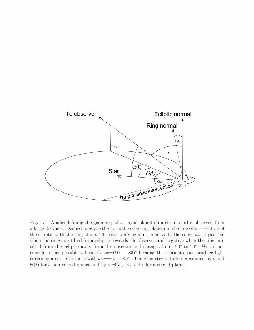
Figure 1 demonstrates the geometry fora ringed planet on a circular orbit defined bythe angles listed in Table 1. The only time-dependent parameters are the orbital angleΘ and phase angle α. For a non-ringed planet the star-planet-observer geometry is fullydetermined by two angles i and Θ (α is linked to i and Θ). For a ringed planet the geometryis determined by four angles: i, Θ, ωr and ǫ.

2.1. Reflecting properties of Jupiter, Saturn and rings

Figure 2 shows the scattered brightness, for a given geometry, derived from our modelfor the surfaces of Jupiter, Saturn, and its the rings in red wavelengths (0.6-0.7µm ). Notethe logarithmic scale of the ordinate and the large amplitudes of the phase functions. Thenormalized brightness I(α, µ0, µ)/(F ·µ0) of a point on the surface is plotted versus scatteringphase angle α. F · µ0 is the “ideal” reflected brightness of a white isotropically scattering

– 6 –

This work Arnold & Quantity UnitsSchneider 2004 (if any)

A,B Coefficients of the Backstorm lawa, a1 Semi-major axis of the planet’s orbit AUDP Planet-star distance kmE Eccentric anomaly (polar angle parameterization)e EccentricityF γ Intensity of a white Lambertian surfacea Wm−2sr−1

g1, g2, f Parameters of Henyey-Greenstein functionI Lp, IR, IT Intensity (or brightness, or radiance) of the surface Wm−2sr−1

Lps, Lpr

i i Inclination of the orbit (0◦: face-on, 90◦: edge-on) degreesLP Luminosity of the planetb Wsr−1

L∗ Luminosity of the starb Wsr−1

M Mean anomaly (time parameterization)p Full-disk albedob LP/(πR

2PF )

R Star’s magnitude in R bandRP rp Equatorial radius of the planet kmrpix Pixel size kmV Star’s magnitude in V bandα α Phase angle degreesǫ Planet’s obliquity degreesΘ φ = Θ− 90◦ Orbital angle (±180◦: min phase, 0◦: max phase) degreesµ0, µ µ0, µ Cosines of the incidence and emission angleω Argument of pericentre(90◦: observed from degrees

pericentre, -90◦: from apocentre)ωr Observer’s azimuth relative to the rings degrees

Table 1: Parameters used in modeling.

aF · (π steradians) is the incident stellar flux at the planet’s orbital distance (which is also sometimes calledF , but has Wm−2 units unlike our intensity F measured per unit solid angle).

bThe ‘red’ or ‘blue’ optical properties are the convolution of the planet’s (or ring’s or solar) spectrum withthe wavelength-dependent transmissivity of the Pioneer filter (which is nonzero between 0.595-0.720µm forred filter and 0.390-0.500µm for blue filter)

– 7 –

Star Θ(t)α(t)

To observer

i

Ring/ecliptic intersection

Ring normal

Ecliptic normal

∋r

Fig. 1.— Angles defining the geometry of a ringed planet on a circular orbit observed froma large distance. Dashed lines are the normal to the ring plane and the line of intersection ofthe ecliptic with the ring plane. The observer’s azimuth relative to the rings, ωr, is positivewhen the rings are tilted from ecliptic towards the observer and negative when the rings aretilted from the ecliptic away from the observer and changes from -90◦ to 90◦. We do notconsider other possible values of ωr=±(90 − 180)◦ because these orientations produce lightcurves symmetric to those with ωr=±(0− 90)◦. The geometry is fully determined by i andΘ(t) for a non-ringed planet and by i, Θ(t), ωr, and ǫ for a ringed planet.

– 8 –

Fig. 2.— Scattering phase functions for a Lambertian surface, Saturn, Jupiter, Saturn’srings (as used in our model), and the phase function for rings consisting of isotropicallyscattering particles used by Arnold & Schneider (2004). The phase functions are plotted fora single sample geometry: µ0 is fixed (the Sun is 2◦ above horizon), while the observer movesin the plane that includes the Sun and zenith. The wavelengths correspond to visible redlight (0.6-0.7µm ).

– 9 –

(Lambertian) surface, where µ0 is the cosine of the incidence angle measured from the localvertical. F · (π steradians) is a solar flux at the planet’s orbital distance. In our notation,α = 0◦ indicates backward scattering and α = 180◦ indicates forward scattering. Lambertianscattering with reflectivity 0.82 (matching Saturn’s full-disk albedo at opposition) is shownas a horizontal solid line for comparison. We also indicate, for the same ring opacity, albedoand geometry, the ring phase function used by Arnold & Schneider (2004), which assumesisotropically-scattering particles.

For Jupiter, we assume that the scattering phase function depends only on α. ForSaturn with rings, the scattering phase function depends on three angles: incidence (via µ0),emission (via µ), and phase (via α), and so cannot be described fully by the one-parameterfunction of α. Figure 2 shows reflected light only for the geometry in which the Sun is2◦ above the horizon (µ0=0.035) and the observer moves from the Sun’s location (α = 0◦)across the zenith toward the point on the horizon opposite to the Sun (α = 178◦). The smallamplitude for isotropically scattering rings in Fig. 2 is due to the very grazing illuminationchosen for this example. At less grazing illuminations, the amplitudes for isotropic rings andour rings are more similar.

2.1.1. Jupiter

For each point on Jupiter, the strong forward scattering of the reflecting clouds isrepresented by the two-term Henyey-Greenstein function P (g1, g2, f, α).

I(α, µ0, µ)/F = µ0 · P (g1, g2, f, α) (1)

P (g1, g2, f, α) = fPHG(g1, α) + (1− f)PHG(g2, α) (2)

The individual terms are Henyey-Greenstein functions representing forward and backwardscattering lobes, respectively.

PHG(g, α) = 2 ·(1− g2)

(1 + g2 + 2g · cosα)3/2, (3)

where α is the phase angle , f is the fraction of the forward versus backward scattering, andg is one of g1 or g2; g1 is positive and controls the sharpness of the forward scattering lobeand g2 is negative and controls the sharpness of the backscattering lobe. Note that we haverewritten PHG relative to common notation in which the scattering angle θ = 180◦−α is used;this reverses the sign in front of the 2g · cosα term. Unlike the common use of the Henyey-Greenstein function for single-particle scattering, in which the function is normalized over thesphere of solid angles around the particle, we use this function only as a convenient analyticalexpression to fit the measured scattering of Jupiter’s surface. In this case, the function isnot normalized over the hemisphere of solid angles above the surface. The spherical albedo(the ratio of reflected to incident light for the whole planet at appropriate wavelengths) is

– 10 –

imbedded in the scattering function, and is a rather complicated integral over the planet’ssurface that we do not calculate here.

Figure 3 shows our fit of the Henyey-Greenstain function, with g1 = 0.8, g2 = −0.38,and f = 0.9, to the data points from the Pioneers 10 and 11 images (Tomasko et al. 1978;Smith & Tomasko 1984). The values we have chosen for g1, g2, and f also reproduce thefull-disk albedos in the spectra observed by Karkoschka (1994) and Karkoschka (1998) at thewavelengths corresponding to the red passband of Pioneer. Pioneer images are taken withbroadband blue (0.390–0.500 µm ) and red (0.595–0.720 µm ) filters at different locations onJupiter. In particular, Tomasko et al. (1978) and Smith & Tomasko (1984) have indicatedtwo types of locations: the belts, usually seen as dark stripes on Jupiter (× symbols on theplot), and zones, usually seen as bright stripes on Jupiter (+ symbols on the plot). Therelative calibration between Pioneer 10 and Pioneer 11 data is not as well constrained as thecalibration within each data set.

Accepting the calibrations given in Tomasko et al. (1978) for Pioneer 10 and Smith &Tomasko (1984) for Pioneer 11, our model curve better represents the observations in thered filter (black data points) than in the blue. We assume here that this curve representsthe red wavelengths. The Pioneer 11 blue data at moderate α in Fig. 3 seem to be system-atically offset from the Pioneer 10 points, which may be a result of relative calibration error.Consequently, we do not model the blue wavelengths.

The vertical spread of the points in the same filter and at the same location is due mainlyto differences in emission and incidence angle between the points. This spread is not large,i.e., the reflectivity is not strongly dependent on incidence and emission angles for fixed αother than a 1/µ0 dependence, which is often labeled “Lambertian limb-darkening.” We note,however, that the Pioneer-measured phase angle dependence is strongly non-Lambertian,which has important consequences for the light curves we generate.

In addition to Pioneer data, images of Jupiter from a variety of angles were takenby Voyager, Galileo, and Cassini, though we are not aware of any other published dataof the scattering phase functions for the Jovian surface.2 Data for α >150◦ do not existbecause these directions would risk pointing spacecraft cameras too close to the Sun; thislimits the ability of the data to constrain the forward-scattering peak at α ∼180◦. Ourderived light curves are not severely affected by this uncertainty, however, since when theforward scattering is important, the observed crescent is small, and reflected light phasecurve undergoes its minimum.

2One of us, UD, plans to work on obtaining the spectral phase functions from Cassini nine-filter visibleimages in the immediate future.

– 11 –

Fig. 3.— Our fit of the Henyey-Greenstein function (solid line, g1 = 0.8, g2 = −0.38,f = 0.9) to the Pioneer 10 data (labeled P10) published as Tables IIa and IIb of Tomaskoet al. (1978), and Pioneer 11 data (labeled P11) published as Tables IIa and IIb of Smith& Tomasko (1984). The data represent belts (dark stripes) and zones (bright stripes) onJupiter observed with the red (0.595–0.720 µm ) and blue (0.390–0.500 µm ) filters.

– 12 –

2.1.2. Saturn

The scattering phase function and albedo of Saturn are represented by the Backstormlaw, which was used by Dones et al. (1993) to fit Saturn’s data.

I/F =A

µ

(

µ · µ0

µ+ µ0

)B

, (4)

where µ and µ0 are the cosines of emission and incident angles measured relative to thelocal vertical, respectively, and A and B are coefficients that depend on the phase angleα. The coefficients are fitted by Dones et al. (1993) to Pioneer 11 fitted phase functiontables, which were produced by the multiple scattering model of Tomasko & Doose (1984).We averaged the coefficients published by Dones et al. (1993) separately for zones and beltsthrough Pioneer’s blue and red filters.

Table 2 gives the resulting coefficients; Fig. 2 displays the red filter curve only.

Phase angle α 0◦ 30◦ 60◦ 90◦ 120◦ 150◦ 180◦a

A (red, 0.64 µm ) 1.69 1.59 1.45 1.34 1.37 2.23 3.09a

B (red, 0.64 µm ) 1.48 1.48 1.46 1.42 1.36 1.34 1.31a

A (blue, 0.44 µm ) 0.63 0.59 0.56 0.56 1.69 1.86 3.03a

B (blue, 0.44 µm ) 1.11 1.11 1.15 1.18 1.20 1.41 1.63a

Table 2: Coefficients for the Backstorm function for Saturn, averaged between belt and zonevalues published in Table V of Dones et al. (1993).

aThe coefficients at α=180◦ are not constrained by observations; and were estimated by linearly extrapolatingthe coefficients at 120◦ and 150◦

The Pioneer spacecraft did not observe Saturn at α > 150◦. Corresponding coefficientsin Dones et al. (1993) are given for α up to 150◦. To complete the phase curve, we extrapolatethe coefficients at 180◦ linearly from their values at 120◦ and 150◦. The phase curve given inFig. 2 corresponds to the case when the incidence angle is fixed at 88◦ (the Sun is 2◦ abovethe horizon, i.e., µ0=0.035) and the trajectory of the observer on the sky is in the planeincluding zenith and Sun’s location (µ is linearly dependent on α). This cross-section of thefitted three-parameter phase function is not as smooth as the Henyey-Greenstein functionfor Jupiter. For example, the dip at α = 90◦ is a result of the approximation by an analyticfunction rather than real observations.

Figure 4 demonstrates the difference between the blue and red phase functions forSaturn. The values for the blue curve are 1.5 − 2 times smaller, indicating that Saturn isdarker in blue wavelengths due to higher absorption by photochemical hazes.

– 13 –

Fig. 4.— Scattering phase functions for Saturn in red (0.595−0.720 µm ) and blue (0.390−0.500 µm ) passbands adopted from Dones et al. (1993).

– 14 –

The ring brightness in reflection (top-side) and transmission (bottom-side) is providedby a physical scattering model of the ring. This model calculates multiple scattering withinthe rings using a ray tracing code. The model ring is populated with macroscopic bodies of1m-size, with optical depth and albedo profiles chosen to match those of Dones et al. (1993).Note that Dones et al. (1993) found the amount of dust in the main rings to be too smallto contribute substantially to ring reflection. The model reproduces well the brightnessesobserved by Voyager 1 and 2. We use the code to predict ring brightness at geometries notobserved by Voyager. The opacity for each pixel is taken at the point on the rings thatprojects to the pixel’s center.

The ring brightness at each point is a function of three angles (α, µ, µ0), the opticaldepth, and the albedo. Due to data volume restrictions we have binned output in ratherlarge steps, which depend on parameter values. These steps are clearly seen in the ringphase function (dotted line) in Fig. 2. The phase function in Fig. 2 corresponds to thesame scattering geometry as the curves for Saturn shown in Fig. 4. The optical depth atthe sample point on the rings (1.7 times Saturn’s radii from the planet’s center) is 2.3, thealbedo of the ring particles is 0.56. The ring is observed from the illuminated side.

To produce light curves of the fiducial exoplanets that we model, images of the planetfor a set of locations along the orbit are generated.

For each image we integrate the total light coming from the planet and the rings (ifany) to obtain the full-disk (or geometric) albedo p(α).

p(α) =

∑

pixels I(µ, µ0, α) · r2pix/F

πR2P

, (5)

where rpix is the pixel size and RP is the planet’s radius. The full-disk albedo is the planet’sluminosity LP normalized by the reflected luminosity of a Lambertian disk with the planet’sradius at the planet’s orbital distance, illuminated and observed from the normal direction.

p ≡ LP/(πR2PF ) (6)

Generally, I, LP , F , and p depend on wavelength. However since we have integrated over thered passband, these values are weighted averages over the Pioneer filter at red wavelengths.

2.2. Eccentric Orbits

In addition to modeling light curves from ringed planets traveling in circular orbits, wealso model the light curves of non-ringed planets moving in eccentric orbits. Although mostof the planets in the Solar system orbit the Sun with low eccentricities, the extrasolar planetsdetected to date display a wide range of eccentricities3.

3Eccentricities of extrasolar planets are listed at http://exoplanets.org/almanacframe.html

– 15 –

Eccentric orbits differ from circular orbits in two main respects. First, the distancebetween the star and the planet varies according to the planet’s orbital position. As theplanet moves from its pericentre to its apocentre, its separation from its host star increases.Second, in an eccentric orbit, the planet does not move with a constant angular speed aroundthe star as it would in a circular orbit. The planet’s angular speed varies throughout theorbit, being a maximum at the pericentre and minimum at the apocentre.

To model the reflected light as a function of time, we calculate the angular position ofthe planet and the planet-star separation over a complete period using a solution to Kepler’sequation (in notation of Murray & Dermott (2001)):

M = E − e sinE (7)

where M is the mean anomaly (a parameterization of time), E is the eccentric anomaly (aparameterization of the polar angle) and e is the eccentricity. Kepler’s equation is transcen-dental in E and therefore cannot be solved directly. Since we need only one complete orbitto model a light curve, however, we are able to use the simple Newton-Ralpson method toobtain a numerical solution to Kepler’s equation. Applying the Newton-Ralpson method4 toEq. 7 we obtain the iterative solution:

Ei+1 = Ei −Ei − e sinEi −Mi

1− e cosEi

(8)

Using this iteration, we calculate the angular position and planet-star separation as functionsof time, and use this to model the amplitude of reflected light from the planet.

As can be seen in Fig. 5, the geometry of an ellipse introduces an additional parame-ter, in addition to inclination, in the observer’s azimuthal perspective of the system. Thisparameter is the argument of pericentre ω, which is the angle (in the planet’s orbital plane)between the ascending node line and pericentre (Murray & Dermott 2001). The referenceplane is formed by the observer’s line of site and its normal in the ecliptic plane, which isalso the accending node line. Viewing the system from the line of the pericentre (planet’ssmallest phase is at pericentre) would give argument of pericentre 90◦. Viewing the systemfrom the line of the apocentre (planet’s largest phase is at pericentre) would give argumentof pericentre −90◦.

3. Results

We modeled several geometries for the planetary system, i.e., different orbital eccen-tricities e for non-ringed planets, and different ring obliquities ǫ relative to the ecliptic for

4Application of Newton-Ralpson method to Kepler’s equation is described in Murray & Dermott (2001)

– 16 –

To observer

PericentreStar

Planet

Fig. 5.— The argument of pericentre, ω, is an additional angle needed to define geometryof a non-ringed planet on eccentric orbit.

ringed planets on circular orbits. For each of these cases we modeled a variety of observerlocations, i.e., different orbital inclinations i as seen by the observer, and different azimuthsω of the observer relative to the orbit’s pericentre or to the rings (ωr). In what follows,we compare light curves for these differing geometries, and discuss whether or not differentgeometric effects can be distinguished from one another from the characteristics of the lightcurve alone.

3.1. Jupiter versus a ringless Saturn

We first tested how light curves would differ for (ringless) exoplanets with the surfacereflection characteristics of Jupiter and Saturn. We modeled the planets for a variety of incli-nations, assuming circular orbits. Low-inclination orbits (close to face-on) produce smallerlight curve amplitudes because the planet appears to be at half-phase most of the time.The most prominent amplitudes, and the most prominent difference between Jupiter andSaturn reflectance properties, occurs for edge-on orbits, for which the phase changes fromcompletely “new moon” to completely “full moon”.

Figure 6 compares edge-on light curves for a ringless Saturn, Jupiter, and a Lambertianplanet. The luminosity of the planet is normalized by the incident stellar illumination toobtain the full-disk albedo p as described in equations (5) and (6). The planets are sphericaland have identical radii; the curves differ only because of the different surface scattering of

– 17 –

Fig. 6.— Comparison of light curves for a spherical Jupiter, a spherical Saturn , and aspherical Lambertian (isotropically scattering) planet, assuming the planets are ringless andhave the same radiiRP . The planets differ only in their surface scattering properties. Albedosare shown for visible red light (0.6-0.7µm ).

– 18 –

the three planets.

The full-disk albedo can be converted into the planet’s luminosity LP as a fraction ofstar’s luminosity L∗ for a planet of equatorial radius RP at an orbital distance DP .

LP/L∗ = (RP/DP )2· p (9)

For example, for Saturn at 1 AU, (RP/DP )2 ≈1.6×10−7. The abscissa of Fig. 6 indicates the

azimuthal angle of the planet in its orbital plane, or the orbital angle Θ (see Fig. 1), startingat minimum planet phase (Θ = −180◦). Note that only for edge-on inclinations does theminimum phase along the orbit correspond to a completely “new moon”. For orbits withlower inclinations, the minimum phase would be a crescent of a size between “new moon” and“half moon”. The corresponding maximum phase will be between the “full moon” and “halfmoon” at Θ = 0◦. For circular orbits, the plot can be transformed into a time-dependentlight curve simply by dividing Θ by 360◦ and multiplying by the planet’s orbital period.

Study of the spectral dependence of reflected light curves is beyond the scope of thispaper; we will address this is a future paper. We do note, however, that Fig. 3 indicatesthat at shorter wavelengths Jupiter is less forward scattering than at longer wavelengths.Also, Figs. 3 and 4 indicate that both Jupiter and Saturn are darker in blue than in red atobservational geometries close to back scattering (α ≈ 0◦).

The light curve for Jupiter peaks much more sharply at full phase (Θ ≈ 0◦) than thelight curves of Saturn or the Lambertian planet because of the sharp back-scattering peak inJupiter’s scattering phase function (α ≈ 0◦ in Fig. 2). Near zero phase (Θ ≈ ±180◦ in Fig.6), Jupiter is more luminous than the other two models due to the large forward scatteringfrom its surface (α ≈ 180◦ in Fig. 2).

Such differences in phase functions is commonly attributed to larger particle size for themain cloud deck on Jupiter. For example, Tomasko et al. (1978) suggest particle sizes largerthan 0.6 µm to explain the forward scattering.

3.2. Oblate Planets

Saturn’s equatorial radius is 10% larger than its polar radius. This 10% oblatenes ofSaturn (6% for Jupiter) makes the planet appear larger when looking from the pole thanwhen looking from the equator, which affects the light curves.

Figure 7 compares light curves for a spherical planet, a 10% oblate planet viewed fromits equator, and a 10% oblate planet viewed from 45◦ latitude. All three sample planetshave the same equatorial radius and scattering properties of Saturn. The light curves inare Fig. 7 are displayed for an edge-on orbit (i=90◦) of a planet rotating “on its side”(ǫ=90◦), because this geometry emphasize the effects of oblateness in the reflected light.The differences among the curves is created by differences in the observer’s azimuth relative

– 19 –

Fig. 7.— Comparison of light curves for a spherical and a 10% oblate planet with Saturn’ssurface properties. Planets have the same equatorial radii and are ringless. The orbit isobserved edge-on (i=90◦). The planets are rotating “on their side” (ǫ=90◦). Albedos shownare for visible red light (0.6-0.7µm ).

– 20 –

to the planet’s equator. (This angle is analogous to ωr but is measured with respect to theequatorial plane rather than the ring plane. The rings are in the equatorial plane for Saturnand thus the same ωr characterizes the observer’s azimuth.) Observing the planet from theequator decreases the cross-section of the planet and thus decreases the amplitude of thecurve. Observing the planet from the pole yields a curve indistinguishable from the solidcurve for a spherical planet; this is not shown in Fig. 7. Observing the planet from latitude45◦ produces a small asymmetry in the curve because on one side of the orbit the flatter(and larger in projection) pole is better illuminated than on the other side of the orbit. Thisasymmetry is small compared to the asymmetries produced by rings, as we discuss in thenext section.

3.3. Ring effects

The presence of rings has a large effect on the light curves of planets in reflected light.In order to describe the geometry of ringed planetary systems, two more parameters are re-quired; even assuming a fixed radial density distribution for the rings, the geometry becomessensitive to the ring obliquity ǫ (the angle between the ring and ecliptic planes), and to theazimuth of the observer relative to the rings ωr (see Fig. 5). Together with the variable or-bital inclination i, this produces the three-parameter space that we have sampled to explorepossible light curves for ringed exoplanets similar to Saturn.

Figure 8 shows an example light curve for i=55◦, ǫ=27◦ and ωr=25◦, which is a conve-nient geometry to demonstrate different ring effects in one light curve. The cartoon on theright of Fig. 8 displays images of Saturn at several positions on the orbit as it would appearto a remote observer. The plot on the left shows the light curve for the ringed planet (+symbols) compared to the curve for the same geometry for a ringless planet (solid curve).The ∼10% spread of the points in the ringed light curve is due partially to the large steps inthe ring reflection table (see Fig. 2) and should be treated as a model uncertainty. For a largefraction of the orbit, the ring presence increases the luminosity of the planet (Θ < −20◦)because the observer is able to view more reflecting surface. However for 0 < Θ < 100◦

the rings are not well illuminated and in fact shadow part of the planet, producing a lowerluminosity than for the non-ringed planet. More importantly, the ringed light curve is asym-metric, which makes it distinguishable from any light curves of a non-ringed planet on acircular orbit. Obviously, planets on eccentric orbits may produce asymmetric curves due tovariation in planet-star separation along the orbit. Light curves for non-ringed planets oneccentric orbits thus could be confused with those of ringed planets in the absence of radialvelocity data (see Section 3.4 for discussion).

The variety of light curves for a Saturn-like planet at different geometries is illustratedin Figure 9. In this figure, different ring’s obliquities are shown in each subplot as blackcurves. The solid black curve indicates an obliquity of ǫ=89◦ (that is, the planet is rotating

– 21 –

Fig. 8.— Effect of Saturn’s rings if observed at 35◦ above the orbital plane (i=55◦). Inthis example, Saturn’s ring’s obliquity is ǫ=27◦. The observer’s azimuth on the ecliptic isseparated from the intersection of the ring and ecliptic planes by ωr=25◦. The plot on theleft shows light curves for a ringless planet (solid curve) and for a ringed planet (crosses).Values of Θ are indicated next to each image. The brightness of the images in the cartoonis given in the units of I/F , as indicated on the nonlinear greyscale bar.

– 22 –

Fig. 9.— Light curves for Saturn for different geometries. Different ring obliquities ǫ areshown on each subplot as black curves. A curve for a spherical planet without rings is shownon each subplot in grey. Each column corresponds to a different orbital inclinations i. Eachrow corresponds to a different azimuth ωr of the observer relative to the rings.

– 23 –

on its side, and rings are located in the equatorial plane and are nearly perpendicular toecliptic). The dotted black curve is for ǫ=45◦, and the dashed black curve is for ǫ=1◦ (ringsare nearly in the ecliptic plane). Grey curves illustrate the same geometries for a non-ringedplanet.

Each subplot within Fig. 9 corresponds to a different observer geometry. In the leftcolumn, the orbit is observed edge-on (i=90◦); the middle column corresponds to an observer45◦ above the ecliptic (i=45◦); the right column shows the orbit observed face-on (i=0◦).Each row corresponds to different azimuths of the observer relative to the rings ωr. Thetop row illustrates geometries with ωr=90◦. At this azimuth, the rings are seen at themaximum possible opening, assuming all other geometric parameters (ring obliquity ǫ andorbital inclination i) are fixed. In lower rows, the observer’s azimuthal is rotated with respectto the orbital plane, resulting in a more grazing view of the rings. The bottom row is forωr=90◦, for which the rings are seen at the most grazing geometry possible for fixed ǫ and i.

Several lessons can be learned from Fig. 9. First, rings generally increase the amplitudeof the light curves by a factor of two to three. Recall that precise, but unresolved observationswill only be able to detect the variations on top of the large constant flux of the star. Anamplitude increase due to rings could be partially confused with effects of due to a largerplanet size or albedo. The ambiguity may be resolved spectrally because the spectrum ofrings should be rather flat, whereas the planetary atmosphere is expected to be dark at aset of prominent gaseous absorption bands.

The second lesson is that light curves for a ringed planet display two types of asymmetry.The first, and potentially easier to detect, asymmetry is the offset of the curve’s maximumrelative to Θ = 0◦, the maximum point for light curves of a ringless planet (marked byvertical lines in Fig. 9). This offset of the light curve maximum itself occurs in rather smallfraction of the plots. However, since the entire curve is asymmetric, the effect would bedetectable as an overall deviation from the simple symmetric curves likely to be used to fitthe first detections of reflected light. If radial velocity data exist for such a planet, the exacttiming of the Θ = 0◦ point and the eccentricity of the orbit would be measurable. In thiscase, a shifted maximum in the light curve would yield direct evidence of the rings whencompared to the asymmetry expected for any orbit eccentricity.

The offset of the light curve maximum due to rings is a strong photometric signature thatwas also noted in the ring simulation of Arnold & Schneider (2004) (as a φ−shift). We stresshere, however, that other processes may be capable of producing such a φ−shift. Similar,although probably smaller, shifts may be induced by seasonal brightness variation on theplanet. None of the giant planets in the Solar System have pronounced seasonal brightnessvariations, but extrasolar planets may display seasons, in which case the variations inducedby them may cause an offset of the brightness maximum. Offsets could also be produced bya global asymmetry of the brightness distribution over the planet. An example in the SolarSystem is the striped appearance of Jupiter. Jupiter’s brightness varies with latitude by as

– 24 –

much as 50% in broadband visible light (Smith & Tomasko 1984). A reasonable scenarioin which an extrasolar planet’s poles are brighter than its equator would cause the planetto appear globally brighter in winter and summer, and darker at mid-seasons, which couldinduce a φ−shift. Oblateness of a planet may also produce a small φ−shift (see Section 3.2).Again, spectroscopy may help to resolve the ambiguity between asymmetries caused by ringsand by processes on the planet surface.

Asymmetry is also apparent in the shape of the light curve, but resolving such detailwould require another order of magnitude in the instrument sensitivity. If this fine structureof the light curves could be measured, however, detection of rings would be possible withoutthe assistance of radial velocity data. The main source of uncertainty in ring detection froman asymmetric light curve is the possibility that the asymmetry is created by an eccentricorbit of the planet. The fine structure of the light curve for the planet on eccentric orbitwould be rather different than the structure for most of the curves for a ringed planet, as wediscuss in Section 3.4.

The third lesson that we can draw from Fig. 9 is that in the case of face-on orbits (rightcolumn), both radial velocity observations and precise photometry would give no signalfor a non-ringed planet. A ringed planet, however, typically produces a double brightnessmaximum, as the rings are illuminated first from the observer’s side and then from the backside during the orbit (dotted curve). At obliquity ǫ = 89◦ (solid curve), the rings are notvisible because the observer is nearly in the ring plane. The observer is also unable to see therings at ǫ = 1◦ (dashed curve) because the star always lies (nearly) in the ring plane. Theseextreme geometries are not typical for the random observations; more typical intermediategeometries (ǫ = 45◦, dotted curve) result in a double peak, which cannot be confused witha light curve for a non-ringed planet on a circular orbit. Only for rare geometries producingequal height of the two peaks, and in the absence of a detailed measurement of the curve’sshape, could these two maximums be confused with a curve for a planet with half the orbitalperiod. Generally, the maximums will differ in height, indicating that both maxima belongto a single orbit. Double maxima can be produced in eccentric orbits, but these exhibitlight curves with differing fine structure (see Section 3.4). We note, however, that a doublepeak may be generated by seasonal variations or by an uneven brightness distribution at theplanet’s surface. For example, a planet with bright poles rotating “on its side” (rotation axisparallel to ecliptic) whose orbit is observed face-on would exhibit two maxima in its lightcurve.

3.4. Effects due to eccentric orbits

One of the primary differences between extrasolar planets discovered to date and thosein the Solar System is the large range of orbital eccentricity displayed by exoplanets. As anexample of the effect eccentricity may have on the light curve of a planet in reflected light,

– 25 –

Figure 10 shows light curves for exoplanet HD 108147b, assuming the equatorial radius andatmospheric properties of Jupiter.

Fig. 10.— Light curves for the planet HD 108147b, assuming Jupiter’s equatorial radius andsurface scattering properties, and 10% oblateness. The argument of pericentre is ω = −41◦.The corresponding time of the maximum phase Θ = 0◦, shown by the vertical line, is ∼ 0.4days after pericentre (which defines time zero). Different orbital inclinations from face-onto edge-on orientations (i=1◦ to i=89◦, respectively) are shown by lines of varying greyness.An edge-on light curve for a planet with Jupiter’s radius but Saturn’s surface properties isshown as a dashed line.

Prescribing Jupiter’s scattering properties to such a close-in planet is a questionableassumption. HD 108147b must be much hotter than Jupiter and may not have clouds at allor may have dark silicate or iron clouds (Sudarsky et al. 2003). Nevertheless, if clouds arepresent on this planet, the scattering of properties of Jupiter may roughly approximate thephase function and yield an order of magnitude estimate of the planet’s brightness (or, more

– 26 –

correctly, an upper limit to the brightness, since Jupiter’s clouds are nearly white).

In Fig. 10, we assume the planet to be 10% oblate, as is Saturn. The planet’s luminosityLP is normalized by the star’s luminosity L∗, and is plotted versus time. We plot the lightcurve over one complete orbit, beginning at pericentre. The orbital parameters are thosedetermined for HD 108147b by precise radial velocity measurements (Pepe et al. 2002).We have chosen to model HD 108147b because of its high eccentricity (e = 0.498) andrelatively short semi-major axis (a = 0.104AU), which accentuates the effects of orbitaleccentricity. Since the inclination of the orbital plane is not determinable from radial velocitymeasurements, we display light curves for different inclinations between i=90◦ (edge-on) andi=0◦ (face-on). The azimuthal location of the pericentre relative to the observer can bederived from the radial velocity measurements. For this HD 108147b, the argument ofpericentre is ω = −41◦, which means that we are fortunate to be at the azimuth at whichthe fullest planet phase Θ = 0◦ is separated from pericentre by only 41◦. With such ageometry, the phase-induced and eccentricity-induced maxima on the light curve amplifyone another. As a result, the amplitude of the curve for the edge-on case is about 3.5×10−5,nearly five times larger than in the face-on case, where only orbital distance variation matters.Because planets with edge-on orbital inclinations are detected more easily via radial velocitymeasurements, the chances of seeing an edge-on planet with a large light curve amplitude infollow-up observations is rather high.

The light curves of Fig. 10 can be rescaled easily for a planet with the same orbitaleccentricity but different semi-major axis a1 by multiplying the luminosity by (a/a1)

2 andmultiplying the time axis by the ratio of the orbital periods (a1/a)

3/2.

In order to illustrate the importance of the argument of pericentre in determining thelight curves of a given system measured by the observer, Figure 11 shows model light curvesfor planet HD 108147b with the same parameters in assumed for Fig. 10, except that theargument of pericentre is now set to ω = 60◦, rather than the true ω = 319◦. This examplealso serves to demonstrate the key features of the light curves for eccentric orbits.

Light curves for orbits observed nearly edge-on (i ≈ 90◦) show a primary peak whenthe planet presents its full phase to the observer. The amplitude of the reflected lightat this peak is approximately LP/L∗=6.5 ×10−6. The amplitude of this primary peak isreduced considerably at lower inclinations, since the planet no longer exhibits full phase atthe maximum phase position. Additionally, the position of this peak moves towards thepericentre as the inclination is lowered.

The edge-on light curve also displays a secondary peak located close to pericentre.This peak is due to the increase in reflected light corresponding to the smaller planet-starseparation at pericentre. At lower inclinations, this secondary peak becomes the higher ofthe two peaks as the planet-star separation function dominates over the phase function. Inthe extreme case of i = 0◦, the phase function no longer affects the light curve (the planetdisplays a constant half phase), and the light curve is purely a function of the planet-star

– 27 –

Fig. 11.— Light curves for a planet with the orbit of HD 108147b, but with an argument ofpericentre ω = 60◦. The planet has the radius and surface scattering properties of Jupiter.The time corresponding to maximum phase is shown by the vertical line, and is ∼ 3.3 daysafter the pericentre. The orbital inclination changes from face-on to edge-on orientations(i=1◦ to i=89◦ respectively), as the line color changes from light grey to black. An edge-onlight curve for same planet, but with Saturn’s surface scattering is shown as a dashed line.

– 28 –

separation.

The i ≈ 90◦ and i = 75◦ light curves are complicated by the appearance of a sharptrough where the amplitude of reflected light is reduced almost to zero. This trough is dueto the planet showing no phase (“new moon”) at this point of its orbit, and is particularlysharp due to the planet’s high angular speed at this point in its orbit. The trough is notprominent in lower inclinations because the minimum phase of the planet is no longer closeto zero.

The double peaks are rather rare; for most values of ω they do not appear at any orbitalinclination. If the planet’s surface is not as forward-scattering as is Jupiter’s ( e.g., Saturn),the second peak is even less likely to appear. However, when the second peak is present, itis necessarily accompanied by the sharp trough immediately next to it. This feature makesthe double-peaked light curve of an eccentric orbit distinguishable from the double-peakedlight curve of a ringed planet, for which the two peaks are broad (see Section 3.3).

Single-peaked curves from eccentric orbits or ringed planets may be distinguished evenwithout radial velocity data because the curve is smooth in the eccentric case. Although bothringed planets and eccentric orbits may result in an asymmetric light curve, the complicatedshadowing of a ringed planet creates abrupt variations along the curve (see Fig. 9).

The location of the light curve maximum relative to the pericentre can yield importantconstraints on the geometry of the orbit and the cloud cover of the planet. First, the orbitalinclination is restricted by the amount of the temporal shift in the light curve maximumfrom pericentre. As the inclination increases, the maximum moves from pericentre (timezero in Figs. 10 and 11) toward the time of the maximum phase Θ = 0◦(the vertical line inFigs. 10 and 11). This shift is larger when the orbit is viewed from a position that placespericentre close to half-phase (ω ∼ 0◦or ω ∼ 180◦) rather than “new moon” (ω ∼ 90◦)or “full-moon” (ω ∼ −90◦) phases. Unlike the amplitude of the curve, which is also anindicator of inclination, the shift cannot be alternatively produced by altering the planet’ssize or albedo. However the shift can result from a different strength of backscattering atthe planet’s surface. An example of such ambiguity is the edge-on light curve for a planetwith Saturn’s scattering properties (dashed line in Fig. 11), which has a maximum wherea Jupiter’s curve of i ≈50◦ would have its maximum. The ambiguity may be resolved bycomparing the detailed shape of the curves.

Second, the curve’s maximum shift may also serve to restrict the surface propertiesof the planet. Although the shift can be confused with the effect of orbital inclination,a lower limit may be put on the strength of backward scattering for the planet’s surface.For each type of scattering surface, a maximum possible shift of the curve’s peak frompericentre towards Θ = 0◦ occurs in the face-on case (i = 0◦). If a larger shift is observed, itcan only be explained by a sharper backward scattering peak of the surface. Constrainingsurface properties in this way should be treated with caution, however, because of possiblecontamination by rings (we did not model both rings and eccentric orbits simultaneously),

– 29 –

large-scale bright patches on the planet’s surface, or seasonal variation of the cloud coverage.

Figure 12 illustrates the sensitivity of the shift to the inclination of the orbit (displayedalong the ordinate of each subplot) and different atmospheric scattering (each of the threecolumns of subplots). The right side of each subplot (ω = −90◦) corresponds to observationsfrom the apocentre side of the orbit. At such a position, the planet is observed at its fullestpossible phase (Θ = 0◦) at pericentre, and since the eccentricity-induced and phase-inducedmaxima in the light curve coincide at pericentre, the shift between the light curve maximumand pericentre is zero. The left side of each subplot (ω = 90◦) corresponds to observationsfrom the pericentre side of the orbit. Here the planet is observed at its smallest possiblephase (Θ = 180◦) at pericentre, so that the eccentricity-induced maximum is shifted fromthe phase-induced maximum by half the orbital period. The maximum of the combinedlight curve then has a complicated dependence on e, i and planet’s scattering properties. Inthe simple case of e = 0, the eccentricity-induced maximum does not exist, and the curve’smaximum is always at the fullest phase. In this case, the time of the maximum follows theobserver’s position ω, with the shift reaching half phase at ω = 90◦ (red at the left on alle = 0 plots).

If radial velocity data exist for the planet, then the orbital eccentricity e and argument ofpericentre ω are known, and the shift, indicated by the color coding in Fig. 12 is observable.The orbital inclination i (shown on the ordinate) is generally not known. Orbital inclinationis known for transiting planets (i ≈ 90◦), but is only very loosely constrained in the absenceof a transit to i < (90 − ∆)◦, where ∆ is a small angle depending on the planet’s size andplanetary system’s geometry.

Our method of constraining the orbital inclination i is achieved by matching a measuredtime shift value with those along the vertical line corresponding to the known ω on the plotwith the appropriate eccentricity, as measured by radial velocity techniques. For example,a planet with Jupiter’s scattering properties on an eccentric e=0.4 orbit, observed to havea temporal shift of 20% of the orbital period (green) by an observer with ω ≈45◦, wouldimply inclinations of 60–90◦. A shift of 10–15% of the orbital period (light blue) would meanorbital inclinations of 30–60◦, while shifts smaller than 10% (purple to black), would meaninclinations of 0–30◦. An ambiguity remains due to the unknown scattering properties of theplanet’s surface. Three examples of the scattering are shown in the three columns of Fig. 12:a strongly backward scattering Jupiter, a weaker backward scattering Saturn, and the lessrealistic extreme case of Lambertian surface. Back scattering stronger than that exhibitedby Jupiter may exist on extrasolar planets. We did not model this case, but expect thatsuch an extreme example would produce a column of plots to the left of the Jupiter column,following the trends back scattering increases from Lambertian on the right to Jupiter onthe left.

Examination of the columns for Jupiter, Saturn and Lambertian surfaces indicates that

– 30 –

Fig. 12.— Summary of the temporal shift of the light curve maximum from the pericentrefor eccentric orbits at different observational geometries for planets with Jupiter-like (leftcolumn), Saturn-like (middle column), and Lambertian scattering properties. Shifts aremeasured as a fraction of the orbital period. Each planet is assumed to be 10% oblate. Theeccentricity of the orbit increases from the top row of subplots to the bottom row. Viewinggeometry is described by the orbital inclination and argument of pericentre, plotted on theordinate and abscissa, respectively of each subplot.

– 31 –

in some cases, scattering properties may be inferred from observation of the temporal shiftin the reflected light. In some geometries a strong temporal shift may be observed at givene and ω. For example, if e = 0.4, ω=60◦, and the observed shift is 25% the orbital period,only the left plot corresponding to Jupiter-like scattering displays green anywhere along theω=60◦ vertical line; thus only strongly back scattering planet like Jupiter can be consistentwith the observation.

The contrast, or difference between the maximum and minimum amplitude of the lightcurve, gives a measure of the degree of variability that the planet’s reflected light displays.It is this variation that new generation space or ground-based photometers may be able todetect if they can achieve the required levels of precision. The largest contrast is observedfor edge-on, i = 90◦, orbits (see Fig. 11), while at lower inclinations the contrast is re-duced. However at very low inclinations approaching i=0◦, the contrast increases again asthe amplitude of reflected light at the pericentre increases. Since the contrast at i=0◦ ishigher than at mid inclinations, measuring reflected light may provide a method of detectingplanets with face-on orbits, so long as the planet’s orbit is highly eccentric. Reflected lightobservations would then complement other methods, such as radial velocity measurements,that are unable to detect planets orbiting with face-on orientations.

We plot the light curve contrast for all possible orbital orientations in Figs. 13. Notethat the backward scattering peak of Jupiter’s surface makes the planet much darker atlow inclinations than Saturn or Lambertian planet. These contour maps display the degreeof contrast for various orbital inclinations and arguments of pericentre at given eccentric-ities. At a given orientation, the more eccentric orbits show much higher contrast thancircular orbits, although the amount of contrast is strongly dependent both on inclinationand argument of pericentre. At high eccentricities, favorable geometries (such as i = 90◦

and ω = −90) can increase the contrast by approximately five times that of less favorableorientations.

4. Discussion

4.1. Uncertainties

Our model provides a rather accurate description of reflected light curves for Jupiterand Saturn. The largest uncertainties are due to the lack of observations at large phaseangles (forward scattering at α >150◦) for the surfaces of Jupiter, Saturn, and its rings.The extrapolations we have made to the phase functions could result in a factor of a fewerror in the brightness at these angles. Luckily, the luminosity of the planet at forward-scattering geometries is small because of the small area of the illuminated crescent at thosepositions. Consequently, this uncertainty does not influence the large amplitude featuresof our modeled light curves. The maxima of the highest-amplitude (edge-on) light curves,

– 32 –

Fig. 13.— Summary of light curve variability amplitudes, or contrast, for eccentric orbitsat different observational geometries for Jupiter (left column), Saturn (middle column),and Lambertian scattering properties with surface albedo 0.82 (right column). Planets areassumed to be 10% oblate.

– 33 –

which happen at opposition, can be constrained to within a few percent by high spectralresolution ground-based data for Saturn and Jupiter. In our study, the uncertainty of thesemaximum amplitudes is 10-20% because the brightness of a planet varies with wavelengthby about the same amount within the 0.6-0.7 µm spectral range (Karkoschka 1998).

Reflectivity of the rings may be in error by as much as 50% because many geometries,especially those for face-on ring illumination and face-on ring observation, are not constrainedby observations. Face-on illumination never happens for Saturn’s rings because of its 27◦

obliquity. Observations of the rings face-on are unavailable because all spacecraft visitingSaturn have had trajectories close to ecliptic. New observations by the Cassini spacecraft(arriving at Saturn in July 2004) will fill this gap in the data. Another source of the ringerror is the coarse grid in the tabulated ring scattering properties (see Section 2). Thisgrid-induced noise is usually below 30% of the ring’s luminosity.

Rings around close-in, short-period exoplanets may be unlikely because of tidal disrup-tion, and in any case can only consist of rock. (Saturn’s rings are 99% ice.) Ice rings are stableagainst evaporation outside ∼7 AU for solar-type stars (Mekler & Podolak 1994). Rockyring material would probably be several times darker than ice, but would remain backwardscattering for geometric reasons. Indeed, the rocks in Saturn’s rings behave as moonlets andare bright at backward-scattering full-phase geometry. Ring density for extrasolar planetsis difficult to predict. It is possible that rocky rings of extrasolar planets are massive andoptically thick. An example in the Solar System is Earth, which may have had massive ringswhile the Moon was forming. Furthermore, ring size for exoplanets may be very differentfrom Saturn’s rings, which would have a large effect on the ring luminosity. We do not modelvarious ring sizes here and refer the reader to the work of Arnold & Schneider (2004) whichinvestigates ring size effects. The optical depth of any rings around extrasolar planets mayalso differ substantially from that of the rings of Saturn. It is important to note that whena ring has an optical depth more than about 3-5, the brightness of illuminated side becomesinsensitive to further increases of optical depth. More than half of the area of Saturn’s ringshas an intermediate optical depth of 0.5-3, which can be considered neither optically thinnor optically thick. These optical depths cause the dark side of Saturn’s ring to be quitebright. If the rings of an extrasolar planet are denser than Saturn’s, the ring-induced lightcurves will be more asymmetric due to the difference between the dark and bright sides ofthe rings. If the rings are optically thin, some asymmetry due to shadows will remain, butthe light curve asymmetry due to the different sides of the ring will decrease. Since most ofSaturn’s rings are quite dense, the brightness of the illuminated side is nearly equal to the“saturated” brightness achieved at infinite optical depth. For this reason, we do not expectthat an increased optical depth in any extrasolar rings will result in a large increase overwhat we predict here in the brightness at the light curve maximum. The effects of differencesin ring size or ring particle albedo are likely to be more prominent.

Application of our model light curves for the bodies of Jupiter and Saturn to the bod-ies of close-in giant exoplanets, whose bright light curves will be the most observable, has

– 34 –

a number of complications related to chemistry. The clouds on these exoplanets are ex-pected to be composed of solid Fe, MgSiO3, Al2O3, and other condensates that are stableat high temperatures (Seager et al. 2000; Burrows & Sharp 1999), rather than the waterand ammonia ices seen in Solar System giants (Weidenschilling & Lewis 1973). This cloudsmay be darker and the corresponding light curve amplitudes may be several times smaller.For spherical particles, the scattering phase function depends on size of the particle com-pared to the wavelength of light, and on particle composition. Consequently, it is possiblethat forward and backward scattering maxima typical of Jupiter and Saturn could occur forcloud-covered exoplanets even if their cloud composition is different. Remarkably, the directspectral signature of ammonia or water ice particles is found in small weather patches thatcover only a few percents of Jupiter’s area (Simon-Miller et al. 2000; Baines et al. 2002).Most of the area is covered by clouds that exhibit no signature of ice on the surface of theparticles. This may be due to the coating of the condensate particles by photochemicallyproduced materials. Whether the photochemistry on extrasolar giant planets could alterthe surface of cloud particles is beyond the scope of this paper, but direct comparison ofclouds made of pure silicate on extrasolar planets, for example, with clouds made of pureammonia on Jupiter and Saturn is probably oversimplified. The most important parameterin determining the brightness of a planet is the presence or absence of clouds, which dependson poorly-known (even for Jupiter and Saturn) vertical atmospheric circulation. Detectionor non-detection of a light curve with the expected amplitudes would be most indicative ofsuch cloud presence.

4.2. Prospects for Detection by Modern Instruments

Short-period giant planets are the easiest targets for detection by precise (spatiallyunresolved) photometry because they are well-illuminated by the star. As discussed in thelast section, light curves for such planets may differ from the those we present here for Jupiterand Saturn because their hotter temperatures (and possibly different evolution as a result ofmigration) will alter the planet’s atmosphere and clouds and thus its scattering properties.

Nevertheless, our model light curves do provide a first-order approximation for a cloud-covered exoplanet and so we will discuss the model light curves of Jupiter and Saturn as ifthey were extrasolar planets placed at small orbital distances. In that case, our light curveamplitudes (Figs. 6 to 9) can be converted to measurable units of fractional luminosityLP/L∗ using Eq. 9. The ratio LP/L∗ depends inversely on the square of the planet’sorbital distance, and is independent of the star’s distance to the observer. Typical extrasolarplanets discovered to date have orbital distances (semi-major axes) between 0.3 and 3 AU,corresponding to conversion factors of 2.5×10−4 to 2.5×10−8 multiplying the order-of-unitylight curve amplitudes displayed in Figs. 6 to 9, assuming that the planet has a radius equalto that of Jupiter’s at 71400 km. For convenience, we have scaled amplitudes in Fig. 13 toa planet with a semi-major axis equal to 1 AU.

– 35 –

The ability of precise space-based photometers such as MOST and KEPLER to detectreflected light from extrasolar planets depends on the signal-to-noise (S/N) of the observa-tions, and thus the apparent brightness of the target parent star. Precisions approaching10−6 are expected for stars as bright as 6th magnitude or brighter in V band (V ≤ 6) withMOST (Green et al. 2003; Walker et al. 2003), and ∼ 67× 10−6 for stars as faint as R = 12in R-band5 with KEPLER (Jenkins & Doyle 2003; Koch et al. 2000; Jenkins et al. 2000;Remund et al. 2001) independent of magnitude. Within a fiducial survey volume of radius30pc, where a solar-type star would have V ≤ 7.2 and R ≤ 6.9, MOST and KEPLER wouldthus be able to provide measurements with precisions of ∼ 2× 10−6 and ∼ 6× 10−6, respec-tively, except where they are dominated by instrumental or stellar noise, which may decreasethe sensitivity by factors of five for the faintest objects. For short-period planets, the S/Nmay be increased by repeated observations over several orbits. On the other hand, planetswith periods longer than the order of several days may suffer more from confusion withfluctuations in stellar luminosity on the order of 10−5 (Jenkins & Doyle 2003). In summary,space-based photometers currently launched such as MOST (with no survey capability) andabout to be launched (KEPLER, a survey instrument), should be able to detect variationsin the total light received from stars within 30pc due to reflected light from orbiting planetsat the level of 10−5.

Direct, spatially-resolved imaging, of the sort that may be provided by future spaceinstruments or adaptive optics on Extremely Large Telescopes (ELT) from the ground (bothaided with coronagraphic or nulling techniques) may detect faint planets if they are suffi-ciently distant from the star to be separable from the angular size of the optical point spreadfunction (Dekany et al. 2004; Lardiere et al. 2003; Codona & Angel 2004; Trauger et al. 2003;Krist et al. 2003; Clampin et al. 2001).

For example, Lardiere et al. (2003) used detailed simulations of ideal adaptive opticssystems with different actuator pitches placed on ground-based ELT of various aperturesizes located in varying atmospheric conditions, to calculate the planet-to-star flux ratiothat would be required in order to reach a signal-to-noise of three (S/N = 3) in one night’sobservation (10 hour exposure). The planet-star flux ratio is related to, but could be slightlylarger than the contrast values of Fig. 13, which show only the varying portion of the planet’sbrightness compared to the (assumed) constant stellar brightness. Generally speaking, theyconclude that a 30m-diameter ELT on one of the best sites in the world ( e.g. Mauna Kea orin the Antarctic) could easily detect with S/N = 3 planets with brightness ratios as small as1× 10−9 over the range of projected planet-host star separations corresponding to 0.1− 1.0arcsec. These separations correspond to planets on orbits with semi-major axes from 1 to10 AU for systems 10pc distant from Earth (and about a factor of ten greater at 30pc).Such planets are more likely to have the temperatures of Saturn and Jupiter, and thus thescattering properties we have assumed here. We note that a ratios of 1× 10−9 is about 100

5We model wavelengths here that are more similar to the R passband than the V band.

– 36 –

times the bright, dark blue contrast levels shown in Fig. 13, indicating that most systemswe have considered would indeed be detectable even if they orbited 10 AU from their host.

Projected onto the sky plane, a planet is most separated from its host star near half-phase, i.e., at Θ ∼ ±90◦ (Figs. 6 to 9). At these points the planet is not at its maximumbrightness, but may still be detectable. Note too that Lambertian planets may underestimateamplitudes at half-phase of planets that scatter anisotropically (see Fig. 6). On the otherhand, rings may increase the luminosity by a factor of 2 − 3 or more if the rings are largerthan those of Saturn, increasing the chance of light curve detection, as would larger planets.Many technical challenges will have to be overcome before contrast levels of 1×10−9 becomedetectable. In this light, it is interesting to note that because planet size is not believed togrow substantially with planet mass above one Jupiter mass (Guillot et al. 1996), searchingfor the photometric signature of large rings of extrasolar planets (if they exist) may be aneasier task than searching for the planets themselves.

– 37 –

5. Conclusions

We have examined the effects of rings, realistic scattering properties ( i.e. those actuallymeasured for Saturn and Jupiter), viewing geometry, and orbit eccentricity on the charac-teristics of reflected light from extrasolar planets, and their combined planet-host star lightcurve. In particular, we have noted signatures of ringed planets, and have indicated cases inwhich planetary rings may be distinguished from, or confused with, other effects.

In the following table, we summarize signatures of planetary rings on the light curves oftheir extrasolar planets, and note differences between ring effects and those of a non-ringedplanet on an eccentric orbit, or planetary surface effects.

Signature Rings Eccentric orbit Alternative

Light curve amplitude increases increase larger albedoby factors 2− 3a depends on e or planet size

Double peak rare rare, sharp trough surface asymmetryb

smooth peaks near one peak or seasons

Large-scale asymmetry common common surface asymmetryb ,oblateness, or seasons

Fine light curve structure abrupt changes smooth

Shift of curve max often never for circular surface asymmetryb ,from Θ=0◦ orbit,calculable oblateness, seasons, or(with radial velocity data) for eccentric orbits back scatteringc

aFor Saturn-sized (relative to the planetary radius) rings.bPlanet-scale asymmetry of the brightness distribution, e.g., bright poles.cThe strengh of the back-scattering peak of the planetary phase function changes the shift of the curvemaximum relative to Θ = 0◦, which is known within the range defined by the possible phase functions (seeFig. 12).

Our studies of planets with Jupiter-like, Saturn-like and Lambertian scattering proper-ties on eccentric orbits hold the following messages for potential observers:

1. An anisotropically scattering planet is much fainter at half-phase (Θ=± 90◦) than isa Lambertian planet.

2. Anisotropically-scattering planets are also much fainter at low inclinations than areLambertian planets.

3. For many geometries, eccentricity of the orbit may increase light curve amplitude by alarge amount compared to a planet on a circular orbit with the same semi-major axis(see Fig. 13)

– 38 –

4. The timing of the lightcurve maximum with respect to pericentre may be used torestrict the orbital inclination and atmospheric back scattering properties for a largefraction of possible geometries (see Fig. 12)

In summary, rings, eccentric orbits, and atmospheric scattering properties of exoplanets maybe detected with future telescopes in the next decade or so by the effect they have on thelight curve of the planet’s reflected light, and these effects may often be distinguished fromone another by the shape of the observed light curve alone or with the aid of additionalradial velocity data.

Acknowledgements

We thank R.A. West for useful references on Jupiter’s scattering. The work begun atNASA GISS while U.D. was supported by Anthony D. Del Genio under the Cassini Project.

REFERENCES

Arnold, L. & Schneider, J. 2004, A&A, accepted

Baines, K. H., Carlson, R. W., & Kamp, L. W. 2002, Icarus, 159, 74

Barnes, J. W. & Fortney, J. J. 2003, Bull.–Am. Astron. Soc., 923

Benedict, G. F., McArthur, B. E., Forveille, T., Delfosse, X., Nelan, E., Butler, R. P.,Spiesman, W., Marcy, G., Goldman, B., Perrier, C., Jefferys, W. H., & Mayor, M.2002, ApJ, 581, L115

Bouchy, F., Pont, F., Santos, N., Melo, C., Mayor, M., Queloz, D., & Udry, S. 2004, A&A,submitted

Burrows, A. & Sharp, C. M. 1999, ApJ, 512, 843

Charbonneau, D., Brown, T. M., Latham, D. W., & Mayor, M. 2000, ApJ, 259, 45

Charbonneau, D., Noues, R., Korzennik, S., Nisenson, P., Jha, S., Vogt, S., & Kibrick, R. I.1999, ApJ, 522, 145

Clampin, M., Ford, H. C., Illingworth, G., Petro, L., & JPF Science Team. 2001, Bulletin ofthe American Astronomical Society, 33, 1356

Codona, J. L. & Angel, R. 2004, ApJ, 604, L117

Collier Cameron, A., Horne, K., Penny, A., & Leigh, C. 2002, MNRAS, 330, 187

– 39 –

Dekany, R., Stapelfeldt, K., Traub, W., Macintosh, B., Woolf, N., Colavita, M., Trauger, J.,& Ftaclas, C. 2004, RASP, submitted

Dones, L., Cuzzi, J., & Showalter, M. 1993, Icarus, 105, 184

Green, D., Mattews, J., Seager, S., & Kuschnig, R. 2003, ApJ, 590

Guillot, T., Burrows, A., Hubbard, W. B., Lunine, J. I., & Saumon, D. 1996, ApJ, 459,L35+

Hatzes, A. P. 2003, in ASP Conference Series, Vol. 294, Scientific Frontiers in Research onExtrasolar Planets, ed. D. Deming & S. Seager (San Francisco: ASP), 523–528

Henry, G. W., Marcy, G. W., Butler, R. P., & Vogt, S. S. 2000, ApJ, 529, L41

Jenkins, J., Witteborn, F., Koch, D., Dunham, E., Borucki, W., Updike, T. F., Skinner, M.,& Jordan, S. 2000, in (SPIE), 520

Jenkins, J. M. & Doyle, L. R. 2003, ApJ, 595, 429

Karkoschka, E. 1994, Icarus, 111, 174

Karkoschka, E. 1998, Icarus, 133, 134

Koch, D., Borucki, W., Dunham, E., Jenkins, J., Webster, L., & Witteborn, F. 2000, in(SPIE), 508

Konacki, M., Torres, G., Jha, S., & Sasselov, D. 2003, Nature, 421, 507

Konacki, M., Torres, G., Sasselov, D., Pietrzynski, G., Udalski, A., Jha, S., Ruiz, M., Gieren,W., & Minniti, D. 2004, ApJ Letters, 609, 37

Krist, J. E., Clampin, M., Petro, L., Woodruff, R. A., Ford, H. C., Illingworth, G. D.,& Ftaclas, C. 2003, in High-Contrast Imaging for Exo-Planet Detection. Edited byAlfred B. Schultz. Proceedings of the SPIE, Volume 4860, pp. 288-294 (2003)., 288–294

Lardiere, O., Salinari, P., Jolissaint, L., Carbillet, M., Riccardi, A., & Esposito, S. 2003, inSecond Backaskog Conference on ELTs (SPIE and ESO)

Leigh, C., Cameron, A. C., & Guillot, T. 2003c, MNRAS, 346, 890

Leigh, C., Cameron, A. C., Horne, K., Penny, A., & James, D. 2003b, MRNAS, 334, 1271

Leigh, C., Collier Cameron, A., Udry, S., Donati, J., Horne, K., James, D., & Penny, A.2003a, MNRAS, 346, L16

Mekler, Y. & Podolak, M. 1994, Planet. Space Sci., 42, 865

– 40 –

Murray, C. D. & Dermott, S. F. 2001, Solar System Dynamics (Cambridge University Press)

Pepe, F., Mayor, M., Galland, F., Naef, D., Queloz, D., Santos, N., Udry, S., & Burnet, M.2002, A & A, 388, 632

Remund, Q., Jordan, S., Updike, T., Jenkins, J., & Borucki, W. 2001, in (SPIE), 182

Seager, S., Whitney, B., & Sasselov, D. 2000, ApJ, 540, 504

Simon-Miller, A. A., Conrath, B. J., Gierasch, P. J., & Beebe, R. F. 2000, Icarus, 145, 454

Smith, P. H. & Tomasko, M. G. 1984, Icarus, 58, 35

Sudarsky, D., Burrows, A., & Hubeny, I. 2003, ApJ, 588, 1121

Tomasko, M. G. & Doose, L. R. 1984, Icarus, 58, 1

Tomasko, M. G., West, R. A., & Castillo, N. D. 1978, Icarus, 33, 558

Trauger, J., Hull, A., Backman, D., Brown, R. A., Burrows, A., Burrows, C., Ealey, M.,Ftaclas, C., Heap, S., Kasdin, J., Kuchner, M., Lindensmith, C., Lunine, J., Marcy,G., Sahai, R., Spergel, D., Stapelfeldt, K., Traub, W., &Woodgate, B. 2003, AmericanAstronomical Society Meeting, 203,

Udalski, A., Paczynski, B., Zebrun, K., Szymaski, M., Kubiak, M., Soszynski, I., Szewczyk,O., Wyrzykowski, L., & Pietrzynski, G. 2002a, Acta Astronomica, 52, 1

Udalski, A., Pietrzynski, G., Szymanski, M., Kubiak, M., Zebrun, K., Soszynski, I.,Szewczyk, O., & Wyrzykowski, L. 2003, Acta Astronomica, 53, 133

Udalski, A., Zebrun, K., Szymanski, M., Kubiak, M., Soszynski, I., Szewczyk, O.,Wyrzykowski, L., & Pietrzynski, G. 2002b, Acta Astronomica, 52, 115

Walker, G., Matthews, J., Kuschnig, R., Johnson, R., Rucinski, S., Pazder, J., Burley, G.,Walker, A., Skaret, K., Zee, R., Grocott, S., Carroll, K., Sinclair, P., Sturgeon, D., &Harron, J. 2003, PASP, 115, 1023

Weidenschilling, S. J. & Lewis, J. S. 1973, Icarus, 20, 465

This preprint was prepared with the AAS LATEX macros v5.2.