Pharmaceutical Supply Chain Networks

with Outsourcing Under Price and Quality Competition

Anna Nagurney1,2, Dong Li1, and Ladimer S. Nagurney3

1Department of Operations and Information Management

Isenberg School of Management

University of Massachusetts, Amherst, Massachusetts 01003

2School of Business, Economics and Law

University of Gothenburg, Gothenburg, Sweden

3 Department of Electrical and Computer Engineering

University of Hartford, West Hartford, CT 06117

January 2013; revised May 2013

International Transactions in Operational Research 20(6) (2013) pp 859-888.

Abstract: In this paper, we present a pharmaceutical supply chain network model with

outsourcing under price and quality competition, in both equilibrium and dynamic versions.

We consider a pharmaceutical firm that is engaged in determining the optimal pharmaceuti-

cal flows associated with its supply chain network activities in the form of manufacturing and

distribution. In addition to multimarket demand satisfaction, the pharmaceutical firm seeks

to minimize its total cost, with the associated function also capturing the firm’s weighted

disrepute cost caused by possible quality issues associated with the contractors. Simulta-

neously, the contractors, who compete with one another in a noncooperative manner in

prices a la Bertrand, and in quality, seek to secure manufacturing and distribution of the

pharmaceutical product from the pharmaceutical firm. This game theory model allows for

the determination of the optimal pharmaceutical product flows associated with the supply

chain in-house and outsourcing network activities and provides the pharmaceutical firm with

its optimal make-or-buy decisions and the optimal contractor-selections. We state the gov-

erning equilibrium conditions and derive the equivalent variational inequality formulation.

We then propose dynamic adjustment processes for the evolution of the product flows, the

quality levels, and the prices, along with stability analysis results. The algorithm yields a

discretization of the continuous-time adjustment processes. We present convergence results

and compute solutions to numerical examples to illustrate the generality and applicability

of the framework.

1

Keywords: outsourcing, pharmaceutical products, healthcare, supply chains, supply chain

networks, quality, competition, game theory, variational inequalities, dynamical systems

2

1. Introduction

Outsourcing is defined as the behavior of moving some of a firm’s responsibilities and/or

internal processes, such as product design or manufacturing, to a third party company

(Chase, Jacobs, and Aquilano (2004)). Outsourcing of manufacturing/production has long

been noted in operations and supply chain management in such industries as computer engi-

neering and manufacturing, financial analysis, fast fashion apparel, and pharmaceuticals (cf.

Austin, Hills, and Lim (2003), Nagurney and Yu (2011), and Hayes et al. (2005)). Evidence

indicates that, in the case of the pharmaceutical industry, outsourcing results in the reduc-

tion of companies’ overall costs (Garofolo and Garofolo (2010)), may increase operational

efficiency and agility (Klopack (2000) and John (2006)), and allows such firms to focus on

their core competitive advantages (Sink and Langley (1997)). In addition, outsourcing may

possibly bring benefits from supportive government policies (Zhou (2007)).

Due to the above noted benefits there is, currently, a tremendous shift from in-house

manufacturing towards outsourcing in US pharmaceutical companies. For example, Pfizer

has increased the outsourcing of its drug manufacturing to 17% from less than 10% (Wheel-

wright and Downey (2008)). In addition, some pharmaceutical firms outsource to multiple

contractors. For example, Bristol-Myers Squibb has had contracts with Celltrion Inc., a Ko-

rean company, and with Lonza Biologics, a Swiss company (Bristol-Myers Squibb (2005)). It

is estimated that the US market for outsourced pharmaceutical manufacturing is expanding

at the rate of 10% to 12% annually (Olson and Wu (2011)). Up to 40% of the drugs that

Americans take are now imported, and more than 80% of the active ingredients for drugs sold

in the United States are outsourced (Economy In Crisis (2010)). Moreover, pharmaceutical

companies are increasingly farming out activities other than production, such as research

and development activities (Higgins and Rodriguez (2006)).

However, the nation’s growing reliance on sometimes uninspected foreign pharmaceutical

suppliers has raised public and governmental awareness and concern, with outsourcing firms

being faced with quality-related risks (Helm (2006), Liu and Nagurney (2011a), and Liu and

Nagurney (2011b)). In 2006, Chinese-made cold medicine contained a toxic substance used

in antifreeze, which can cause death (Bogdanich and Hooker (2007)). In 2008, fake heparin

made by one Chinese manufacturer not only led to recalls of drugs in over ten European

countries (Payne (2008)), but also caused the deaths of 81 American citizens (The New York

Times (2011)). Given the growing volume of global outsourcing, quality issues in outsourced

products must be of paramount concern, especially since adulterated pharmaceuticals, which

are ingested, may negatively affect a patient’s recovery or may even result in loss of life.

3

Although the need for regulations for the quality control of overseas pharmaceuticals and

ingredients is urgent, due to the limited resources of the US Food and Drug Administration

(FDA) that are available for global oversight, pharmaceutical firms, as well as citizens, can-

not rely on the FDA to ensure the quality of outsourced pharmaceuticals (The New York

Times (2011)). At the same time, pharmaceutical firms are under increasing pressure from

consumers, the government, the medical insurance industry, and even the FDA, to reduce

the prices of their pharmaceuticals (Enyinda, Briggs, and Bachkar (2009)). Thus, phar-

maceutical companies must be prepared to adopt best practices aimed at safeguarding the

quality of their supply chain networks. A more comprehensive supply chain network model

that captures contractor selection, the minimization of the disrepute of the pharmaceutical

firm, as well as the competition among contractors, is an imperative.

In this paper, we develop a pharmaceutical supply chain network model utilizing a game

theory approach which takes into account the quality concerns in the context of global

outsourcing. This model captures the behaviors of the pharmaceutical firm and its potential

contractors with consideration of the transactions between them and the quality of the

outsourced pharmaceutical product. The objective of each contractor is to maximize its total

profit. The pharmaceutical firm seeks to minimize its total cost, which includes its weighted

disrepute cost, which is influenced by the quality of the product produced by its contractors

and the amount of product that is outsourced. The contractors compete with one another

by determining the prices that they charge the pharmaceutical firm for manufacturing and

delivering the product to the demand markets and the quality levels in order to maximize

their profits.

We now provide a review of the relevant literature. We first note that only a small

portion of the supply chain literature directly addresses and models the risk of quality and

safety issues associated with outsourcing. Kaya (2011) considered an outsourcing model in

which the supplier makes the quality decision and an in-house production model in which the

manufacturer decides on the quality. Kaya and Ozer (2009) employed vertical integration

in their three-stage decision model to determine how the original equipment manufacturer’s

pricing strategy affects quality risk. The above two papers both used an effort function

to capture the cost of quality in outsourcing. Balakrishnan, Mohan, and Seshadri (2008)

considered quality risk in outsourcing as a recent supply chain phenomenon of outsourcing

front-end business processes. In addition, Gray, Roth, and Tomlin (2008) proposed a metric

of quality risk based on real data from the drug industry and provided empirical evidence

that unobservability of quality risk causes the contract manufacturer to shirk on quality.

Obviously, in global manufacturing outsourcing, contractors do not only do production,

4

but also are responsible for the sourcing of raw materials and conducting quality-related

tasks such as inspections and incoming and outgoing quality control. They determine the

quality of the materials that they purchase as well as the standard of their manufacturing

activities. However, contract manufacturers may have less reason to be concerned with the

quality (Amaral, Billington, and Tsay (2006)), since they may not have the same priorities

as the original firms when making decisions about and trade-offs between cost and quality,

which may lead them to expend less effort to ensure high quality.

Hence, quality should be quantified and incorporated into the make-or-buy, as well as the

contractor-selection decision of pharmaceutical firms. If a contractor’s poor quality product

negatively affects the pharmaceutical firm’s reputation, then outsourcing to that contractor

will not be a wise choice.

Quality costs are defined as “costs incurred in ensuring and assuring quality as well as

the loss incurred when quality is not achieved” (ASQC (1971) and BS (1990)). There are a

variety of schemes by which quality costing can be implemented in organizations, as described

in Juran and Gryna (1988) and Feigenbaum (1991). Based on the literature of quality cost,

four categories of quality-related costs occur in the process of quality management, and are

widely applied in organizations (see, e.g., Crosby (1979), Harrington (1987), Plunkett and

Dale (1988), Juran and Gryna (1993), and Rapley, Prickett, and Elliot (1999)). They are

prevention costs, appraisal costs, internal failure costs, and external failure costs. Quality

cost is usually understood as the sum of the four categories of quality-related costs. Moreover,

it is widely believed that the functions of the four quality-related costs are convex functions

of the quality conformance level, which varies from a 0% defect-free level to a 100% defect-

free level (see, e.g., Juran and Gryna (1988), Campanella (1990), Feigenhaum (1983), Porter

and Rayner (1992), and Shank and Govindarajan (1994)).

The game theory supply chain network model developed in this paper is based on the

following assumptions:

1. The pharmaceutical firm may contract the manufacturing and the delivery tasks to the

contractors.

2. According to regulations (FDA (2002), U.S. Department of Health and Human Services,

CDER, FDA, and CBER (2009), and the European Commission Health and Consumers

Directorate (2010)) and the literature, before signing the contract, the pharmaceutical firm

should have reviewed and evaluated the contractors’ ability to perform the outsourcing tasks.

Therefore, the production/distribution costs and the quality cost information of the contrac-

tors are assumed to be known by the firm.

5

3. In addition to paying the contractors, the pharmaceutical firm also pays the transaction

cost and one category of the quality-related costs, the external failure costs. The transaction

cost is the “cost of making each contract” (cf. Coase (1937) and also Aubert, Rivard,

and Patry (1996)), which includes the costs of evaluating suppliers, negotiation costs, the

monitoring and the enforcement of the contract in order to ensure the quality (Picot (1991),

Franceschini (2003), Heshmati (2003), and Liu and Nagurney (2011a)). External failure

costs are the compensation costs incurred when customers are unsatisfied with the quality of

the products. The objective of the pharmaceutical firm is to minimize the total operational

costs and transaction costs, along with the weighted individual disrepute.

4. For the in-house supply chain activities, it is assumed that the pharmaceutical firm can

ensure a 100% perfect quality conformance level (see Schneiderman (1986) and Kaya (2011)).

5. The contractors, who produce for the same pharmaceutical firm, compete a la Bertrand

(cf. Bertrand (1838)) by determining their optimal prices and quality levels in order to

maximize their profits.

We develop both a static version of the model (at the equilibrium state) and also a

dynamic one using the theory of projected dynamical systems (cf. Nagurney and Zhang

(1996)). In our earlier research on pharmaceutical supply chain networks (cf. Masoumi, Yu,

and Nagurney (2012)), we focused on Cournot competition (cf. Cournot (1838)), where firms

selected their optimal product flows under perishability of the pharmaceutical product, and

we did not consider outsourcing. Moreover in that work, the underlying dynamics were not

identified. This paper adds to the growing literature on supply chain network equilibrium

problems introduced by Nagurney, Dong, and Zhang (2002) (see also Nagurney et al. (2002),

Dong, Zhang, and Nagurney (2004), Dong et al. (2005), and Cruz (2008)), with the inclusion

of contractor behavior, Bertrand competition in prices, as well as quality competition, and

dynamics.

This paper is organized as follows. In Section 2, we describe the decision-making behavior

of the pharmaceutical firm and the competing contractors. We then develop the game theory

model, state the equilibrium conditions, and derive the equivalent variational inequality

formulation. We assume that the demand for the pharmaceutical product is known at

the various demand markets since the pharmaceutical firm can be expected to have good

in-house forecasting abilities. Hence, we focus on cost minimization associated with the

pharmaceutical firm but profit maximization for the contractors who compete on prices and

quality.

In Section 3, we provide a dynamic version of the model through a description of the

6

underlying adjustment processes associated with the product flows, the quality levels, and

the contractor prices. We show that the projected dynamical system has stationary points

that coincide with the solutions for relevant corresponding the variational inequality problem.

We also provide stability analysis results.

In Section 4, we describe the algorithm, which yields closed form expressions, at each

iteration, for the contractor prices and the quality levels, with the product flows being

solved exactly using an equilibration algorithm. The algorithm provides a discrete-time

version of the continuous-time adjustment processes given in Section 3. We illustrate the

concepts through small examples, and include sensitivity analysis results. We then apply

the algorithm in Section 5 to demonstrate the modeling and computational framework on

larger examples. We explore the case of a disruption in the pharmaceutical supply chain

network and two cases focused on opportunity costs. We summarize our results and give our

conclusions in Section 6.

7

2. The Pharmaceutical Supply Chain Network Model with Outsourcing and

Price and Quality Competition

In this section, we develop the pharmaceutical supply chain network model with out-

sourcing and with price and quality competition among the contractors. We assume that

a pharmaceutical firm is involved in the processes of in-house manufacturing and distribu-

tion of a pharmaceutical product, and may also contract its manufacturing and distribution

activities to contractors, who may be located overseas. We seek to determine the optimal

product flows of the firm to its demand markets, along with the prices the contractors charge

the firm for production and distribution, and the quality levels of their products.

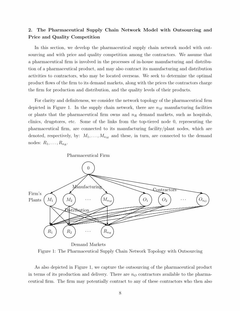
For clarity and definiteness, we consider the network topology of the pharmaceutical firm

depicted in Figure 1. In the supply chain network, there are nM manufacturing facilities

or plants that the pharmaceutical firm owns and nR demand markets, such as hospitals,

clinics, drugstores, etc. Some of the links from the top-tiered node 0, representing the

pharmaceutical firm, are connected to its manufacturing facility/plant nodes, which are

denoted, respectively, by: M1, . . . ,MnMand these, in turn, are connected to the demand

nodes: R1, . . . , RnR.

����Pharmaceutical Firm

0

���

���

�����

����

M1

Firm’s

Plants

?

����

R1

@@@@@R

PPPPPPPPPPPPPPPq

��

���

����

M2

Manufacturing

Distribution

?

����

R2

Demand Markets

��

���

HHHHHHHHHHj

· · ·

· · ·

@@@@@R

����MnM

?

����RnR

���������������)

�����������

PPPPPPPPPPPPPPPq

����

O1

��������������������

����������

XXXXXXXXXXXXXXXXXXXXz

����

O2

���������������)

· · ·

hhhhhhhhhhhhhhhhhhhhhhhhhhhhhhz

����OnO

Contractors

Figure 1: The Pharmaceutical Supply Chain Network Topology with Outsourcing

As also depicted in Figure 1, we capture the outsourcing of the pharmaceutical product

in terms of its production and delivery. There are nO contractors available to the pharma-

ceutical firm. The firm may potentially contract to any of these contractors who then also

8

distribute the outsourced product that they manufacture to the nR demand markets. The

first set of outsourcing links directly link the top-most node 0 to the nO contractor nodes,

O1, . . . , OnO, which correspond to their respective manufacturing activities, and the next set

of outsourcing links emanate from the contractor nodes to the demand markets and reflect

the delivery of the outsourced pharmaceutical product to the demand markets.

Let G = [N ,L] denote the graph consisting of nodes [N ] and directed links [L] as in

Figure 1. The top set of links consists of the manufacturing links, whether in-house or

outsourced (contracted), whereas the next set of links consists of the distribution links. For

simplicity, we let n = nM +nO denote the number of manufacturing plants, whether in-house

or belonging to the contractors. The notation for the model is given in Table 1. The vectors

are assumed to be column vectors. The optimal/equilibrium solution is denoted by “∗”.

Table 1: Notation for the Game Theoretic Supply Chain Network Model with OutsourcingNotation Definition

Qjk the nonnegative amount of pharmaceutical product produced at man-ufacturing plant j and delivered to demand market k.We group the {Qjk} elements into the vector Q ∈ RnnR

+ .dk the demand for the product at demand market k, assumed known

and fixed.

qj the nonnegative quality level of the pharmaceutical product producedby contractor j. We group the {qj} elements into the vector q ∈ RnO

+ .πjk the price charged by contractor j for producing and delivering a unit

of the product to k. We group the {πjk} elements for contractor jinto the vector πj ∈ RnR

+ and then group all such vectors for all thecontractors into the vector π ∈ RnOnR .

fj(∑nR

k=1 Qjk) the total production cost at manufacturing plant j; j = 1, . . . , nM

owned by the pharmaceutical firm.q′ the average quality level.

tcj(∑nR

k=1 QnM+j,k) the total transaction cost associated with the firm transacting withcontractor j; j = 1, . . . , nO.

cjk(Qjk) the total transportation cost associated with delivering the productmanufactured at j to k; j = 1, . . . , nM ; k = 1, . . . , nR.

scjk(Q, q) the total cost of contractor j; j = 1, . . . , nO, to produce and distributethe product to demand market k; k = 1, . . . , nR.

qcj(q) quality cost faced by contractor j; j = 1, . . . , nO.ocjk(πjk) the opportunity cost associated with pricing the product by contrac-

tor j; j = 1, . . . , nO and delivering it to k; k = 1, . . . , nR.dc(q′) the cost of disrepute, which corresponds to the external failure quality

cost.

9

2.1 The Behavior of the Pharmaceutical Firm

Since quality is a major issue in the pharmaceutical industry and, hence, it is the industry

selected to focus on in our model, we first discuss how we capture quality. We assume

that in-house activities can ensure a 100% perfect quality conformance level. The quality

conformance level of contractor j is denoted by qj, which varies from a 0% defect-free level

to a 100% defect-free level, such that

0 ≤ qj ≤ qU , j = 1, . . . , nO, (1)

where qU is the value representing perfect quality achieved by the pharmaceutical firm in its

in-house manufacturing.

The quality level associated with the product of the pharmaceutical firm is, hence, an

average quality level that is determined by the quality levels decided upon by the contractors

and the outsourced product amounts. Thus, the average quality level for the pharmaceutical

firm’s product, both in-house and outsourced, can be expressed as

q′ =∑n

j=nM+1

∑nR

k=1 Qjkqj−nM+ (

∑nM

j=1

∑nR

k=1 Qjk)qU∑nR

k=1 dk

. (2)

The pharmaceutical firm selects the product flows Q, whereas the contractors, who compete

with one another, select their respective quality level qj and price vector πj for contractor

j = 1, . . . , nO.

Since we are presenting a game theory model, we use terms from game theory.

The objective of the pharmaceutical firm is to maximize its utility (cf. (3) below), repre-

sented by minus its total costs that include the production costs, the transportation costs,

the payments to the contractors, the total transaction costs, along with the weighted cost

of disrepute, with the nonnegative term ω denoting the weight that the firm imposes on the

disrepute cost function. The firm’s utility function is denoted by U0 and, hence, the firm

seeks to

MaximizeQ U0(Q, q∗, π∗) = −nM∑j=1

fj(

nR∑k=1

Qjk)−nM∑j=1

nR∑k=1

cjk(Qjk)−nO∑j=1

nR∑k=1

π∗jkQnM+j,k

−nO∑j=1

tcj(

nR∑k=1

QnM+j,k)− ωdc(q′). (3)

subject to:n∑

j=1

Qjk = dk, k = 1, . . . , nR, (4)

10

Qjk ≥ 0, j = 1, . . . , n; k = 1, . . . , nR, (5)

with q′ in (3) as in (2).

Note that (3) is equivalent to minimizing the total costs. Also, according to (4) the

demand at each demand market must be satisfied. This is important since the firm is

dealing with pharmaceutical products. We assume that all the cost functions in (3) are

continuous, continuously differentiable, and convex. We define the feasible set K0 as follows:

K0 ≡ {Q|Q ∈ RnnR+ with (4) satisfied}. K0 is closed and convex. The following theorem is

immediate.

Theorem 1

The optimality conditions for the pharmaceutical firm, faced with (3) and subject to (4)

and (5), with q′ as in (2) embedded into dc(q′), and under the above imposed assumptions,

coincide with the solution of the following variational inequality (cf. Nagurney (1999) and

Bazaraa, Sherali, and Shetty (1993)): determine Q∗ ∈ K0

−n∑

h=1

nR∑l=1

∂U0(Q∗, q∗, π∗)

∂Qhl

× (Qhl −Q∗hl) ≥ 0, ∀Q ∈ K0, (6)

with notice that: for h = 1, . . . , nM ; l = 1, . . . , nR:

− ∂U0

∂Qhl

=

[∂fh(

∑nR

k=1 Qhk)

∂Qhl

+∂chl(Qhl)

∂Qhl

+ ω∂dc(q′)∂Qhl

]

=

[∂fh(

∑nR

k=1 Qhk)

∂Qhl

+∂chl(Qhl)

∂Qhl

+ ω∂dc(q′)

∂q′qU∑nR

k=1 dk

],

and for h = nM + 1, . . . , n; l = 1, . . . , nR:

− ∂U0

∂Qhl

=

[π∗h−nM ,l +

∂tch−nM(∑nR

k=1 Qhk)

∂Qhl

+ ω∂dc(q′)∂Qhl

]

=

[π∗h−nM ,l +

∂tch−nM(∑nR

k=1 Qhk)

∂Qhl

+ ω∂dc(q′)

∂q′q∗h∑nR

k=1 dk

].

2.2 The Behavior of the Contractors and Their Optimality Conditions

The objective of the contractors is profit maximization. Their revenues are obtained

from the purchasing activities of the pharmaceutical firm, while their costs are the costs of

production and distribution, the quality cost, and the opportunity cost. Opportunity cost is

defined as “the loss of potential gain from other alternatives when one alternative is chosen”

11

(New Oxford American Dictionary, 2010). In this model, the contractors’ opportunity costs

are functions of the prices charged, since, if the values are too low, they may not recover all

of their costs, whereas if they are too high, then the firm may select another contractor. In

our model, these are the only costs that depend on the prices that the contractors charge

the pharmaceutical firm and, hence, there is no double counting. We note that the concept

of opportunity cost (cf. Mankiw (2011)) is very relevant to both economics and operations

research. It has been emphasized in pharmaceutical firm competition by Grabowski and

Vernon (1990), Palmer and Raftery (1999), and Cockburn (2004). Gan and Litvinov (2003)

also constructed opportunity cost functions that are functions of prices as we consider here

(see Table 1) but in an energy application.

Interestingly, Leland (1979), inspired by the work of the Nobel laureate Akerlof (1970)

on quality, noted that drugs (pharmaceuticals) must satisfy federal safety standards and, in

his model, introduced opportunity costs that are functions of quality levels.

We emphasize that general opportunity cost functions include both explicit and implicit

costs (Mankiw (2011)) with the explicit opportunity costs requiring monetary payment, and

including possible anticipated regulatory costs, wage expenses, and the opportunity cost of

capital (see Porteus (1986)), etc. Implicit opportunity costs are those that do not require

payment, but to the decision-maker, still need to be monetized, for the purposes of decision-

making, and can include the time and effort put in (see Payne, Bettman, and Luce (1996)),

and the profit that the decision-maker could have earned, if he had made other choices

(Sandoval-Chavez and Beruvides (1998)).

Please note that, as presented in Table 1, scjk(Q, q), which is contractor j’s cost function

associated with producing and delivering the pharmaceutical firm’s product to demand mar-

ket k, only captures the cost of production and delivery. It depends on both the quantities

and the quality levels. However, qcj(q) is the cost associated with quality management, and

reflects the “cost incurred in ensuring and assuring quality as well as the loss incurred when

quality is not achieved,” and is over and above the cost of production and delivery activities.

As indicated in the Introduction, qcj(q) is a convex function in the quality levels. Thus,

scjk(Q, q) and qcj(q) are two entirely different costs, and they do not overlap.

Each contractor has, as its strategic variables, its quality level, and the prices that it

charges the pharmaceutical firm for production and distribution to the demand markets.

We denote the utility of each contractor j by Uj, with j = 1, . . . , nO, and note that it

12

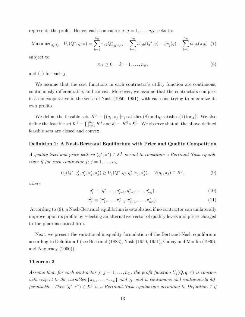
represents the profit. Hence, each contractor j; j = 1, . . . , nO seeks to:

Maximizeqj ,πjUj(Q

∗, q, π) =

nR∑k=1

πjkQ∗nM+j,k −

nR∑k=1

scjk(Q∗, q)− qcj(q)−

nR∑k=1

ocjk(πjk) (7)

subject to:

πjk ≥ 0, k = 1, . . . , nR, (8)

and (1) for each j.

We assume that the cost functions in each contractor’s utility function are continuous,

continuously differentiable, and convex. Moreover, we assume that the contractors compete

in a noncooperative in the sense of Nash (1950, 1951), with each one trying to maximize its

own profits.

We define the feasible sets Kj ≡ {(qj, πj)|πj satisfies (8) and qj satisfies (1) for j}. We also

define the feasible set K1 ≡∏nO

j=1 Kj and K ≡ K0×K1. We observe that all the above-defined

feasible sets are closed and convex.

Definition 1: A Nash-Bertrand Equilibrium with Price and Quality Competition

A quality level and price pattern (q∗, π∗) ∈ K1 is said to constitute a Bertrand-Nash equilib-

rium if for each contractor j; j = 1, . . . , nO

Uj(Q∗, q∗j , q

∗j , π

∗j , π

∗j ) ≥ Uj(Q

∗, qj, q∗j , πj, π∗j ), ∀(qj, πj) ∈ Kj, (9)

where

q∗j ≡ (q∗1, . . . , q∗j−1, q

∗j+1, . . . , q

∗nO

), (10)

π∗j ≡ (π∗1, . . . , π∗j−1, π

∗j+1, . . . , π

∗nO

). (11)

According to (9), a Nash-Bertrand equilibrium is established if no contractor can unilaterally

improve upon its profits by selecting an alternative vector of quality levels and prices charged

to the pharmaceutical firm.

Next, we present the variational inequality formulation of the Bertrand-Nash equilibrium

according to Definition 1 (see Bertrand (1883), Nash (1950, 1951), Gabay and Moulin (1980),

and Nagurney (2006)).

Theorem 2

Assume that, for each contractor j; j = 1, . . . , nO, the profit function Uj(Q, q, π) is concave

with respect to the variables {πj1, . . . , πjnR} and qj, and is continuous and continuously dif-

ferentiable. Then (q∗, π∗) ∈ K1 is a Bertrand-Nash equilibrium according to Definition 1 if

13

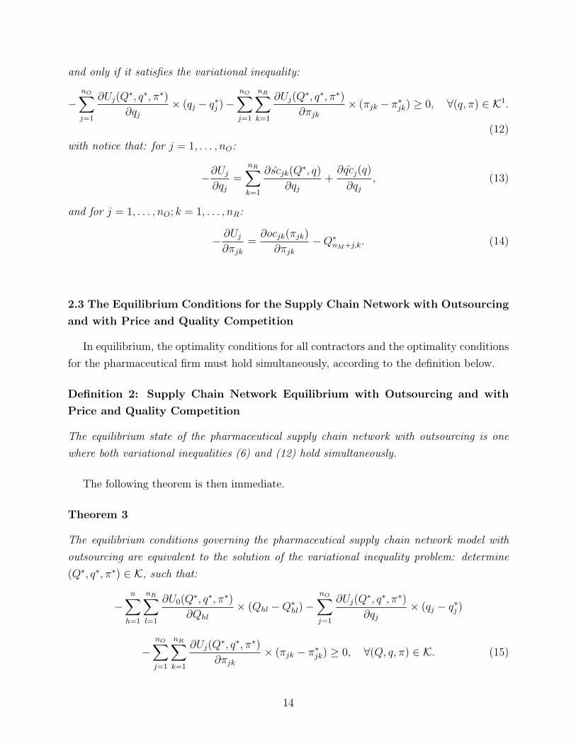
and only if it satisfies the variational inequality:

−nO∑j=1

∂Uj(Q∗, q∗, π∗)

∂qj

× (qj − q∗j )−nO∑j=1

nR∑k=1

∂Uj(Q∗, q∗, π∗)

∂πjk

× (πjk − π∗jk) ≥ 0, ∀(q, π) ∈ K1.

(12)

with notice that: for j = 1, . . . , nO:

−∂Uj

∂qj

=

nR∑k=1

∂scjk(Q∗, q)

∂qj

+∂qcj(q)

∂qj

, (13)

and for j = 1, . . . , nO; k = 1, . . . , nR:

− ∂Uj

∂πjk

=∂ocjk(πjk)

∂πjk

−Q∗nM+j,k. (14)

2.3 The Equilibrium Conditions for the Supply Chain Network with Outsourcing

and with Price and Quality Competition

In equilibrium, the optimality conditions for all contractors and the optimality conditions

for the pharmaceutical firm must hold simultaneously, according to the definition below.

Definition 2: Supply Chain Network Equilibrium with Outsourcing and with

Price and Quality Competition

The equilibrium state of the pharmaceutical supply chain network with outsourcing is one

where both variational inequalities (6) and (12) hold simultaneously.

The following theorem is then immediate.

Theorem 3

The equilibrium conditions governing the pharmaceutical supply chain network model with

outsourcing are equivalent to the solution of the variational inequality problem: determine

(Q∗, q∗, π∗) ∈ K, such that:

−n∑

h=1

nR∑l=1

∂U0(Q∗, q∗, π∗)

∂Qhl

× (Qhl −Q∗hl)−nO∑j=1

∂Uj(Q∗, q∗, π∗)

∂qj

× (qj − q∗j )

−nO∑j=1

nR∑k=1

∂Uj(Q∗, q∗, π∗)

∂πjk

× (πjk − π∗jk) ≥ 0, ∀(Q, q, π) ∈ K. (15)

14

We now put variational inequality (15) into standard form (cf. Nagurney (1999)): de-

termine X∗ ∈ K where X is a vector in RN , F (X) is a continuous function such that

F (X) : X 7→ K ⊂ RN , and

〈F (X∗), X −X∗〉 ≥ 0, ∀X ∈ K, (16)

where 〈·, ·〉 is the inner product in the N -dimensional Euclidean space, and K is closed and

convex. We define the vector X ≡ (Q, q, π). Also, here N = nnR + nO + nOnR. Note that

(16) may be rewritten as:

N∑i=1

Fi(X∗)× (Xi −X∗

i ) ≥ 0, ∀X ∈ K. (17)

The components of F are then as follows. The first nnR components of F are given

by: −∂U0(Q,q,π)∂Qhl

for h = 1, . . . , n; l = 1, . . . , nR; the next nO components of F are given

by: −∂Uj(Q,q,π)

∂qjfor j = 1, . . . , nO, and the subsequent nOnR components of F are given by:

−∂Uj(Q,q,π)

∂πjkwith j = 1, . . . , nO; k = 1, . . . , nR. Hence, (15) can be put into standard form

(16).

15

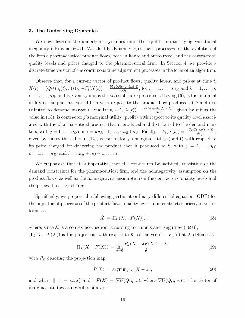
3. The Underlying Dynamics

We now describe the underlying dynamics until the equilibrium satisfying variational

inequality (15) is achieved. We identify dynamic adjustment processes for the evolution of

the firm’s pharmaceutical product flows, both in-house and outsourced, and the contractors’

quality levels and prices charged to the pharmaceutical firm. In Section 4, we provide a

discrete-time version of the continuous time adjustment processes in the form of an algorithm.

Observe that, for a current vector of product flows, quality levels, and prices at time t,

X(t) = (Q(t), q(t), π(t)), −Fi(X(t)) = ∂U0(Q(t),q(t),π(t))∂Qhl

, for i = 1, . . . , nnR and h = 1, . . . , n;

l = 1, . . . , nR, and is given by minus the value of the expressions following (6), is the marginal

utility of the pharmaceutical firm with respect to the product flow produced at h and dis-

tributed to demand market l. Similarly, −Fi(X(t)) =∂Uj(Q(t),q(t),π(t))

∂qj, given by minus the

value in (13), is contractor j’s marginal utility (profit) with respect to its quality level associ-

ated with the pharmaceutical product that it produced and distributed to the demand mar-

kets, with j = 1, . . . , nO and i = nnR+1, . . . , nnR+nO. Finally, −Fi(X(t)) =∂Uj(Q(t),q(t),π(t))

∂πjk,

given by minus the value in (14), is contractor j’s marginal utility (profit) with respect to

its price charged for delivering the product that it produced to k, with j = 1, . . . , nO;

k = 1, . . . , nR, and i = nnR + nO + 1, . . . , n.

We emphasize that it is imperative that the constraints be satisfied, consisting of the

demand constraints for the pharmaceutical firm, and the nonnegativity assumption on the

product flows, as well as the nonnegativity assumption on the contractors’ quality levels and

the prices that they charge.

Specifically, we propose the following pertinent ordinary differential equation (ODE) for

the adjustment processes of the product flows, quality levels, and contractor prices, in vector

form, as:

X = ΠK(X,−F (X)), (18)

where, since K is a convex polyhedron, according to Dupuis and Nagurney (1993),

ΠK(X,−F (X)) is the projection, with respect to K, of the vector −F (X) at X defined as

ΠK(X,−F (X)) = limδ→0

PK(X − δF (X))−X

δ(19)

with PK denoting the projection map:

P(X) = argminz∈K‖X − z‖, (20)

and where ‖ · ‖ = 〈x, x〉 and −F (X) = ∇U(Q, q, π), where ∇U(Q, q, π) is the vector of

marginal utilities as described above.

16

We now further interpret ODE (18) in the context of the supply chain network game

theory model with price and quality competition among the contractors. Observe that ODE

(18) guarantees that the product flows, quality levels, and the contractor prices are always

nonnegative and that the demand constraints (4) are also satisfied. If one were to consider,

instead, the ordinary differential equation: X = −F (X), or, equivalently, X = ∇U(X),

such an ODE would not ensure that X(t) ≥ 0, for all t ≥ 0, unless additional restrictive

assumptions were to be imposed. Moreover, it would not be guaranteed that the demand

at the demand markets would be satisfied and that the upper bound on the quality levels

would be met.

Recall now the definition of F (X) for the model, which captures the behavior of all

the decision-makers in the supply chain network with outsourcing and competition in an

integrated manner. The projected dynamical system (18) states that the rate of change of

the product flows, quality levels, and contractor prices is greatest when the pharmaceutical

firm’s and contractors’ marginal utilities are greatest. If the marginal utility of a contractor

with respect to its quality level is positive, then the contractor will increase its quality level;

if it is negative, then it will decrease the quality. Note that the quality levels will also never

be outside their upper bound. A similar adjustment behavior holds for the contractors in

terms of the prices that they charge, but without an upper bound on the prices. This type

of behavior is rational from an economic standpoint. Therefore, ODE (18) corresponds to

reasonable continuous adjustment processes for the supply chain network game theory model

with outsourcing and quality and price competition.

Although the use of the projection on the right-hand side of ODE (18) guarantees that the

underlying variables are always nonnegative, and that the other constraints are satisfied, it

also raises the question of existence of a solution to ODE (18), since this ODE is nonstandard

due to its discontinuous right-hand side. Dupuis and Nagurney (1993) constructed the

fundamental theory with regards to existence and uniqueness of projected dynamical systems

as defined by (18). We cite the following theorem from that paper. See also the book by

Nagurney and Zhang (1996). For a plethora of dynamic, multitiered supply chain network

models under Cournot competition, see the book by Nagurney (2006).

Theorem 4

X∗ solves the variational inequality problem (15), equivalently, (16), if and only if it is a

stationary point of the ODE (18), that is,

X = 0 = ΠK(X∗,−F (X∗)). (21)

17

This theorem provides the necessary and sufficient condition for a pattern X∗ = (Q∗, q∗, π∗)

to be an equilibrium, according to Definition 2, in that X∗ = (Q∗, q∗, π∗) is a stationary point

of the adjustment processes defined by ODE (18), that is, X∗ is the point at which X = 0.

3.1 Stability Under Monotonicity

We now turn to the questions as to whether and under what conditions does the adjust-

ment processes defined by ODE (21) approach an equilibrium? We first note that Lipschitz

continuity of F (X) (cf. Dupuis and Nagurney (1993) and Nagurney and Zhang (1996)) guar-

antees the existence of a unique solution to (22) below, where we have that X0(t) satisfies

ODE (18) with product flow, quality level, and price pattern (Q0, q0, π0). In other words,

X0(t) solves the initial value problem (IVP)

X = ΠK(X,−F (X)), X(0) = X0, (22)

with X0(0) = X0. For convenience, we sometimes write X0 · t for X0(t).

We present the following definitions of stability for these adjustment processes, which are

adaptations of those introduced in Zhang and Nagurney (1995). Hereafter, we use B(X, r)

to denote the open ball with radius r and center X.

Definition 3

An equilibrium product flow, quality level, and price pattern X∗ is stable, if for any ε > 0,

there exists a δ > 0, such that for all initial X ∈ B(X∗, δ) and all t ≥ 0

X(t) ∈ B(X∗, ε). (23)

The equilibrium point X∗ is unstable, if it is not stable.

Definition 4

An equilibrium product flow, quality level, and price pattern X∗ is asymptotically stable, if

it is stable and there exists a δ > 0 such that for all initial product flows, quality levels, and

prices X ∈ B(X∗, δ)

limt→∞

X(t) −→ X∗. (24)

18

Definition 5

An equilibrium product flow, quality level, and price pattern X∗ is globally exponentially

stable, if there exist constants b > 0 and µ > 0 such that

‖X0(t)−X∗‖ ≤ b‖X0 −X∗‖e−µt, ∀t ≥ 0, ∀X0 ∈ K. (25)

Definition 6

An equilibrium product flow, quality level, and price pattern X∗ is a global monotone attrac-

tor, if the Euclidean distance ‖X(t)−X∗‖ is nonincreasing in t for all X ∈ K.

Definition 7

An equilibrium X∗ is a strictly global monotone attractor, if ‖X(t) −X∗‖ is monotonically

decreasing to zero in t for all X ∈ K.

We now tackle the stability of the adjustment processes under various monotonicity con-

ditions.

Recall (cf. Nagurney (1999)) that F (X) is monotone if

〈F (X)− F (X∗), X −X∗〉 ≥ 0, ∀X, X∗ ∈ K. (26)

F (X) is strictly monotone if

〈F (X)− F (X∗), X −X∗〉 > 0, ∀X, X∗ ∈ K, X 6= X∗. (27)

F (X) is strongly monotone X∗, if there is an η > 0, such that

〈F (X)− F (X∗), X −X∗〉 ≥ η‖X −X∗‖2, ∀X, X∗ ∈ K. (28)

The monotonicity of a function F is closely related to the

positive-definiteness of its Jacobian ∇F (cf. Nagurney (1999)). Specifically, if ∇F is

positive-semidefinite, then F is monotone; if ∇F is positive-definite, then F is strictly

monotone; and, if ∇F is strongly positive-definite, in the sense that the symmetric part

of ∇F, (∇F T +∇F )/2, has only positive eigenvalues, then F is strongly monotone.

In the context of our supply chain network game theory model with outsourcing, where

F (X) is the vector of negative marginal utilities as follows (17), we note that if the utility

19

functions are twice differentiable and the Jacobian of the negative marginal utility functions

(or, equivalently, the negative of the Hessian matrix of the utility functions) for the integrated

model is positive-definite, then the corresponding F (X) is strictly monotone.

We now present an existence and uniqueness result, the proof of which follows from the

basic theory of variational inequalities (cf. Nagurney (1999)).

Theorem 5

Suppose that F is strongly monotone. Then there exists a unique solution to variational

inequality (16); equivalently, to variational inequality (15).

The following theorem summarizes the stability properties of the utility gradient pro-

cesses, under various monotonicity conditions on the marginal utilities.

Theorem 6

(i). If F (X) is monotone, then every supply chain network equilibrium, as defined in Defini-

tion 2, provided its existence, is a global monotone attractor for the utility gradient processes.

(ii). If F (X) is strictly monotone, then there exists at most one supply chain network equi-

librium. Furthermore, given existence, the unique equilibrium is a strictly global monotone

attractor for the utility gradient processes.

(iii). If F (X) is strongly monotone, then the unique supply chain network equilibrium, which

is guaranteed to exist, is also globally exponentially stable for the utility gradient processes.

Proof: The stability assertions follow from Theorems 3.5, 3.6, and 3.7 in Nagurney and

Zhang (1996), respectively. The uniqueness in (ii) is a classical variational inequality result,

whereas existence and uniqueness as in (iii) follows from Theorem 5. 2

20

4. The Algorithm

As mentioned in Section 3, the projected dynamical system yields continuous-time ad-

justment processes. However, for computational purposes, a discrete-time algorithm, which

serves as an approximation to the continuous-time trajectories is needed.

We now recall the Euler method, which is induced by the general iterative scheme of

Dupuis and Nagurney (1993). Specifically, iteration τ of the Euler method (see also Nagurney

and Zhang (1996)) is given by:

Xτ+1 = PK(Xτ − aτF (Xτ )), (29)

where PK is the projection on the feasible set K and F is the function that enters the

variational inequality problem (16).

As shown in Dupuis and Nagurney (1993) and Nagurney and Zhang (1996), for conver-

gence of the general iterative scheme, which induces the Euler method, the sequence {aτ}must satisfy:

∑∞τ=0 aτ = ∞, aτ > 0, aτ → 0, as τ →∞. Specific conditions for convergence

of this scheme as well as various applications to the solutions of other game theory models

can be found in Nagurney, Dupuis, and Zhang (1994), Nagurney, Takayama, and Zhang

(1995), Cruz (2008), Nagurney (2010), and Nagurney and Li (2012).

We emphasize that this is the first time that this algorithm is being adapted and ap-

plied for the solution of supply chain network game theory problems under Nash-Bertrand

competition and with outsourcing.

Note that, at each iteration τ , Xτ+1 in (29) is actually the solution to the strictly con-

vexquadratic programming problem given by:

Xτ+1 = MinimizeX∈K1

2〈X, X〉 − 〈Xτ − aτF (Xτ ), X〉. (30)

As for solving (30) in order to obtain the values of the product flows at each iteration

τ , we can apply the exact equilibration algorithm, originated by Dafermos and Sparrow

(1969) and applied to many different applications of networks with special structure (cf.

Nagurney (1999) and Nagurney and Zhang (1996)). See also Nagurney and Zhang (1997)

for an application to fixed demand traffic network equilibrium problems.

Furthermore, in light of the nice structure of the underlying feasible set K, we can ob-

tain the values for the quality variables explicitly according to the following closed form

21

expressions for contractor j; j = 1, . . . , nO:

qτ+1j = min{qU , max{0, qτ

j + aτ (−nR∑k=1

∂scjk(Qτ , qτ )

∂qj

−∂qcj(q

τ )

∂qj

)}}. (31)

Also, we have the following explicit formulae for the contractor prices: for j = 1, . . . , nO;

k = 1, . . . , nR:

πτ+1jk = max{0, πτ

jk + aτ (−∂ocjk(π

τjk)

∂πjk

+ QτnM+j,k)}. (32)

We now provide the convergence result. The proof is direct from Theorem 5.8 in Nagurney

and Zhang (1996).

Theorem 7

In the supply chain network model with outsourcing, let F (X) = −∇U(Q, q, π) be strongly

monotone. Also, assume that F is uniformly Lipschitz continuous. Then there exists a unique

equilibrium product flow, quality level, and price pattern (Q∗, q∗, π∗) ∈ K and any sequence

generated by the Euler method as given by (29) above, where {aτ} satisfies∑∞

τ=0 aτ = ∞,

aτ > 0, aτ → 0, as τ →∞ converges to (Q∗, q∗, π∗).

Note that convergence also holds if F (X) is monotone (cf. Theorem 8.6 in Nagurney and

Zhang (1996)) provided that the price iterates are bounded. We know that the product flow

iterates as well as the quality level iterates will be bounded due to the constraints. Clearly,

in practice, contractors cannot charge unbounded prices for production and delivery. Hence,

we can also expect the existence of a solution, given the continuity of the functions that

make up F (X), under less restrictive conditions that that of strong monotonicity.

4.1 An Illustrative Example, a Variant, and Sensitivity Analysis

We now provide a small example to clarify ideas, along with a variant, and also conduct a

sensitivity analysis exercise. The supply chain network consists of the pharmaceutical firm,

a single contractor, and a single demand market, as depicted in Figure 2.

The data are as follows. The firm’s production cost function is:

f1(Q11) = Q211 + Q11

and its total transportation cost function is:

c11(Q11) = .5Q211 + Q11.

22

����Pharmaceutical Firm

0

?����M1Firm’s Plant

?����R1

Demand Market

@@@@R����O1

����

Contractor

Figure 2: Supply Chain Network for an Illustrative Numerical Example

The firm’s transaction cost function associated with the contractor is given by:

tc1(Q21) = .05Q221 + Q21.

The demand for the pharmaceutical product at demand market R1 is 1,000 and qU is 100

and the weight ω is 1.

The contractor’s total cost of production and distribution function is:

sc11(Q21, q1) = Q21q1.

Its total quality cost function is given by:

qc1(q1) = 10(q1 − 100)2.

The contractor’s opportunity cost function is:

oc11(π11) = .5(π11 − 10)2.

The pharmaceutical firm’s cost of disrepute function is:

dc(q′) = 100− q′

where q′ (cf. (1)) is given by: Q21q1+Q111001000

.

We set the convergence tolerance to 10−3 so that the algorithm was deemed to have

converged when the absolute value of the difference between each product flow, each quality

level, and each price was less than or equal to 10−3. So, in effect, a stationary point had been

23

achieved. The Euler method was initialized with Q011 = Q0

21 = 500, q01 = 1, and π0

11 = 0.

The sequence {aτ} was set to: {1, 12, 1

2, 1

3, 1

3, 1

3, . . .}.

The Euler method converged in 87 iterations and yielded the following product flow,

quality level, and price pattern:

Q∗11 = 270.50, Q∗21 = 729.50, q∗1 = 63.52, π∗11 = 739.50.

The total cost incurred by the pharmaceutical firm is 677,128.65 with the contractor earning

a profit of 213,786.67. The value of q′ is 73.39.

The Jacobian matrix of F (X) = −∇U(Q, q, π), for this example, denoted by J(Q11, Q21,

q1, π11), is

J(Q11, Q21, q1, π11) =

3 0 0 00 .1 −.001 10 1 20 00 −1 0 1

.

This Jacobian matrix is positive-definite, and, hence, -∇U(Q, q, π) is strongly monotone

(see also Nagurney (1999)). Thus, both the existence and the uniqueness of the solution

to variational inequality (15) with respect to this example are guaranteed. Moreover, the

equilibrium solution, reported above, is globally exponentially stable.

We then constructed a variant of this example. The transportation cost function was

reduced by a factor of 10 so that it is now:

c11(Q11) = .05Q211 + .1Q11

with the remainder of the data as in the original example above. This could capture the

situation of the firm moving its production facility closer to the demand market.

The Euler method again required 87 iterations for convergence and yielded the following

equilibrium solution:

Q∗11 = 346.86, Q∗21 = 653.14, q∗1 = 67.34, π∗11 = 663.15.

The pharmaceutical firm’s total costs are now 581,840.07 and the contractor’s profits are

165,230.62. The value of q′ is now 78.67. The average quality increased, with the quantity of

the product produced by the firm having increased. Also, the price charged by the contractor

decreased but the quality level of its product increased.

For both the examples, the underlying constraints are satisfied, consisting of the demand

constraint, the nonnegativity constraints, as well as the upper bound on the contractor’s

quality level. In addition, the variational inequality for this problem is satisfied.

24

It is easy to verify that the Jacobian of F for the variant is positive-definite with the only

change in the Jacobian matrix above being that the 3 is replaced by 2.1.

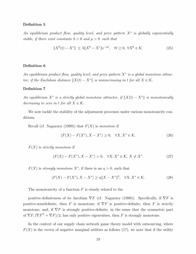
We then proceeded to conduct a sensitivity analysis exercise. We returned to the original

example and increased the demand for the pharmaceutical product at R1 in increments of

1,000. The results of the computations are reported in Figures 3, 4, and 5 for the equilibrium

product flows, the quality levels and the average quality q′, and, finally, the equilibrium

prices.

Figure 3: Equilibrium Product Flows as the Demand Increases for the Illustrative Example

25

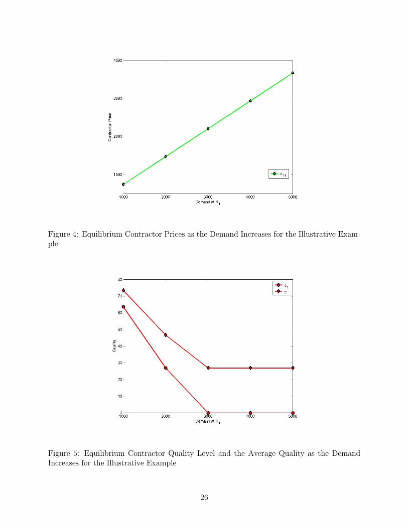
Figure 4: Equilibrium Contractor Prices as the Demand Increases for the Illustrative Exam-ple

Figure 5: Equilibrium Contractor Quality Level and the Average Quality as the DemandIncreases for the Illustrative Example

26

It is interesting to observe that, when the demand increased past a certain point, the

contractor’s equilibrium quality level decreased to zero and stayed at that level. Such unex-

pected insights may be obtained through a modeling and computational framework that we

have developed. Of course, the results in this subsection are based on constructed examples.

One may, of course, conduct other sensitivity analysis exercises and also utilize different

underlying cost functions in order to tailor the general framework to specific pharmaceutical

firms’ needs and situations.

5. Additional Numerical Examples

In this section, we applied the Euler method to compute solutions to examples that are

larger than those in the preceding section. We report all of the input data as well as the

output. The Euler method was initialized as in the illustrative example, except that the

initial product flows were equally distributed among the available options for each demand

market. We used the same convergence tolerance as previously.

Example 1 and Sensitivity Analysis

Example 1 consists of the topology given in Figure 6. There are two manufacturing plants

owned by the pharmaceutical firm and two possible contractors. The firm must satisfy the

demands for its pharmaceutical product at the two demand markets. The demand for the

pharmaceutical product at demand market R1 is 1,000 and it is 500 at demand market R2.

qU is 100 and the weight ω is 1.

����0

Pharmaceutical Firm

����

���

����Firm’s Plants M1

?

����R1

@@@R

���

����M2

?

����R2

Demand Markets

���

@@@R

����O1���������)

�������

HHHHHHj

����O2 Contractors������������9

���������)

Figure 6: Supply Chain Network Topology for Example 1

The production cost functions at the plants are:

f1(2∑

k=1

Q1k) = (Q11 + Q12)2 + 2(Q11 + Q12), f2(

2∑k=1

Q2k) = 1.5(Q21 + Q22)2 + 2(Q21 + Q22).

27

The total transportation cost functions are:

c11(Q11) = 1.5Q211 + 10Q11, c12(Q12) = 1Q2

12 + 25Q12,

c21(Q21) = 1Q221 + 5Q21, c22(Q22) = 2.5Q2

22 + 40Q22.

The transaction cost functions are:

tc1(Q31+Q32) = .5(Q31+Q32)2+.1(Q31+Q32), tc2(Q41+Q42) = .25(Q41+Q42)

2+.2(Q41+Q42).

The contractors’ total cost of production and distribution functions are:

sc11(Q31, q1) = Q31q1, sc12(Q32, q1) = Q32q1,

sc21(Q41, q2) = 2Q41q2, sc22(Q42, q2) = 2Q42q2.

Their total quality cost functions are given by:

qc1(q1) = 5(q1 − 100)2, qc2(q2) = 10(q1 − 100)2.

The contractors’ opportunity cost functions are:

oc11(π11) = .5(π11 − 10)2, oc12(π12) = (π12 − 10)2,

oc21(π21) = (π21 − 5)2, oc22(π22) = .5(π22 − 20)2.

The pharmaceutical firm’s cost of disrepute function is:

dc(q′) = 100− q′

where q′ (cf. (1)) is given by: Q31q1+Q32q1+Q41q2+Q42q2+Q11100+Q12100+Q21100+Q221001500

.

The Euler method converged in 153 iterations and yielded the following equilibrium so-

lution. The computed product flows are:

Q∗11 = 95.77, Q∗12 = 85.51, Q∗21 = 118.82, Q∗22 = 20.27,

Q∗31 = 213.59, Q∗32 = 224.59, Q∗41 = 571.83, Q∗42 = 169.63.

The computed quality levels of the contractors are:

q∗1 = 56.18, q∗2 = 25.85,

28

and the computed prices are:

π∗11 = 223.57, π∗12 = 122.30, π∗21 = 290.92, π∗22 = 189.61.

The total cost of the pharmaceutical firm is 610,643.26 and the profits of the contractors

are: 5,733.83 and 9,294.44.

The value of q′ is 50.55.

In order to investigate the stability of the computed equilibrium for Example 1 (and a

similar analysis holds for the subsequent examples), we constructed the Jacobian matrix

as follows. The Jacobian matrix of F (X) = −∇U(Q, q, π), for this example, denoted by

J(Q11, Q12, Q21, Q22, Q31, Q32, Q41, Q42, q1, q2, π11, π12, π21, π22), is

J(Q11, Q12, Q21, Q22, Q31, Q32, Q41, Q42, q1, q2, π11, π12, π21, π22)

=

5 2 0 0 0 0 0 0 0 0 0 0 0 02 4 0 0 0 0 0 0 0 0 0 0 0 00 0 5 3 0 0 0 0 0 0 0 0 0 00 0 3 8 0 0 0 0 0 0 0 0 0 00 0 0 0 1 1 0 0 −6.67× 10−4 0 1 0 0 00 0 0 0 1 1 0 0 −6.67× 10−4 0 0 1 0 00 0 0 0 0 0 0.5 0.5 0 −6.67× 10−4 0 0 1 00 0 0 0 0 0 0.5 0.5 0 −6.67× 10−4 0 0 0 10 0 0 0 0 0 0 0 10 0 0 0 0 00 0 0 0 0 0 2 2 0 20 0 0 0 00 0 0 0 −1 0 0 0 0 0 1 0 0 00 0 0 0 0 −1 0 0 0 0 0 2 0 00 0 0 0 0 0 −1 0 0 0 0 0 2 00 0 0 0 0 0 0 −1 0 0 0 0 0 1

.

This Jacobian matrix is positive-semidefinite. Hence, according to Theorem 6 we know

that, since F (X) is monotone, every supply chain network equilibrium, as defined in Defini-

tion 2, is a global monotone attractor for the utility gradient process.

Interestingly, in this example, the pharmaceutical firm pays relatively higher prices for

the products with a lower quality level from contractor O2. This happens because the firm’s

demand is fixed in each demand market, and, therefore, there is no pressure for quality

improvement from the demand side (as would be the case if te demands were elastic (cf.

Nagurney and Li (2012)). As reflected in the transaction costs with contractors O1 and O2,

the pharmaceutical firm is willing to pay higher prices to O2, despite a lower quality level.

We then conducted sensitivity analysis. In particular, we investigated the effect of in-

creases in the demands at both demand markets R1 and R2. The results for the new equi-

29

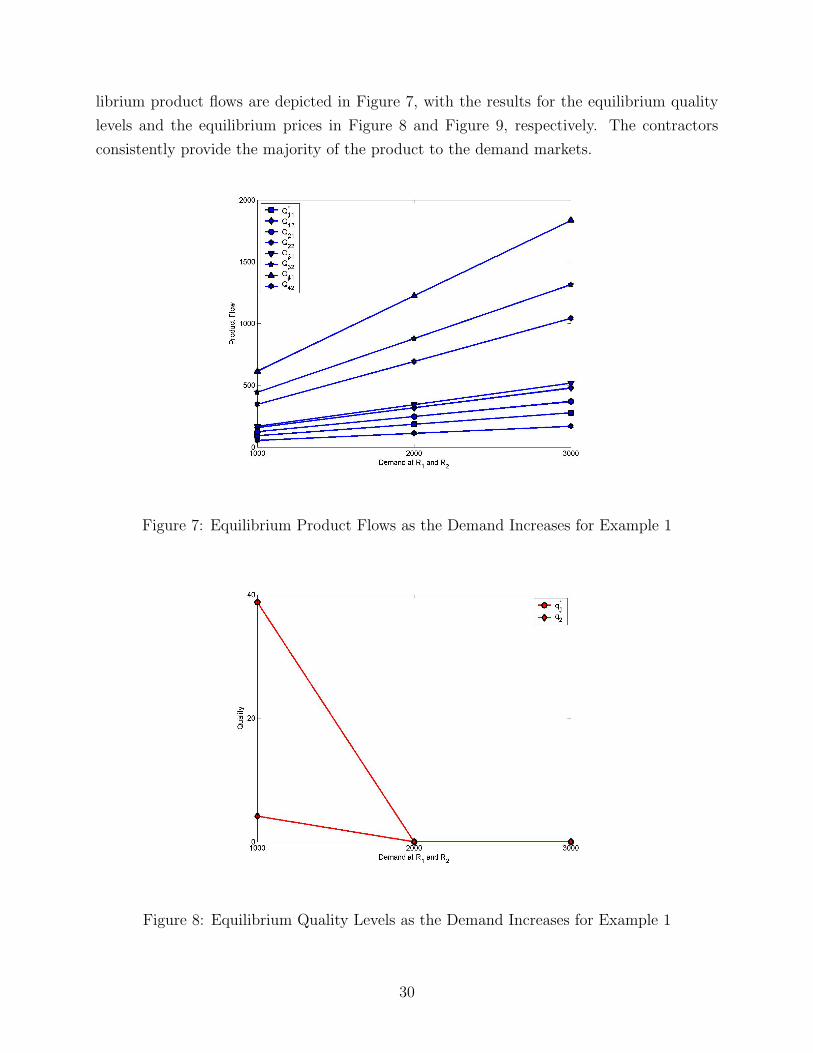
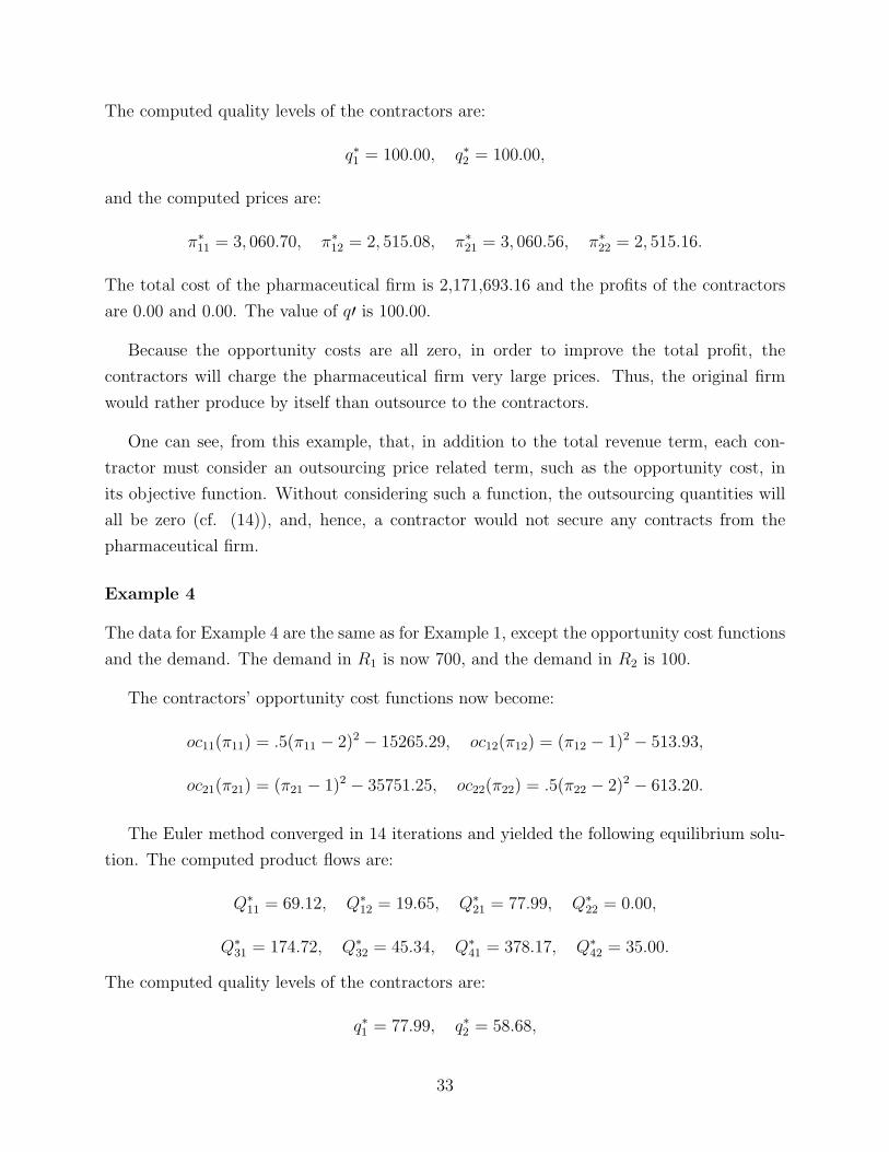
librium product flows are depicted in Figure 7, with the results for the equilibrium quality

levels and the equilibrium prices in Figure 8 and Figure 9, respectively. The contractors

consistently provide the majority of the product to the demand markets.

Figure 7: Equilibrium Product Flows as the Demand Increases for Example 1

Figure 8: Equilibrium Quality Levels as the Demand Increases for Example 1

30

Figure 9: Equilibrium Contractor Prices as the Demand Increases for Example 1

Observe from Figure 8 that as the demand increases the quality levels for both contractors

drops to zero.

Example 2

We then considered a disruption to the original supply chain in Example 1. No business

is immune from supply chain disruptions and, as noted by Purtell (2010), pharmaceuticals

are especially vulnerable since they are high-value, highly regulated products. Moreover,

pharmaceutical disruptions may not only increase costs but may also create health hazards

and expose the pharmaceutical companies to damage to their brands and reputations (see

also Nagurney, Yu, and Qiang (2011), Masoumi, Yu, and Nagurney (2012), and Qiang and

Nagurney (2012)).

Specifically, we considered the following disruption. The data are as in Example 1 but

contractor O2 is not able to provide any production and distribution services. This could

arise due to a natural disaster, adulteration in its production process, and/or an inability to

procure an ingredient. Hence, the topology of the disrupted supply chain network is as in

Figure 10.

The Euler method converged in 73 iterations and yielded the following new equilibrium

31

����0

Pharmaceutical Firm

���

����

����Firm’s Plants M1

?

����R1

@@@R

���

����M2

?

����R2

Demand Markets

���

@@@R

����O1���������)

��

��

���

Contractor

Figure 10: Supply Chain Network Topology for Example 2

solution. The computed product flows are:

Q∗11 = 218.06, Q∗12 = 141.79, Q∗21 = 260.20, Q∗22 = 25.96, Q∗31 = 521.74, Q∗32 = 332.25.

The computed quality level of the remaining contractor is:

q∗1 = 14.60,

and the computed prices are:

π∗11 = 531.74, π∗12 = 176.12.

With the decrease in competition among the contractors, since there is now only one,

rather than two, as in Example 1, the quality level of contractor O1 dropped, but the prices

that it charged increased. The new average quality level is q′=51.38. The total cost of the

pharmaceutical firm is now 1,123,226.62 whereas the profit of the first contractor is now

123,460.67, a sizable increase relative to that with competition as in Example 1.

Example 3

The data for Example 3 are the same as for Example 1, except that the opportunity cost

functions oc11, oc12, oc21, oc22 are all equal to 0.00.

The Euler method converged in 76 iterations and yielded the following equilibrium solu-

tion. The computed product flows are:

Q∗11 = 451.17, Q∗12 = 396.50, Q∗21 = 548.73, Q∗22 = 103.39,

Q∗31 = 0.00, Q∗32 = 0.00, Q∗41 = 0.00, Q∗42 = 0.00.

32

The computed quality levels of the contractors are:

q∗1 = 100.00, q∗2 = 100.00,

and the computed prices are:

π∗11 = 3, 060.70, π∗12 = 2, 515.08, π∗21 = 3, 060.56, π∗22 = 2, 515.16.

The total cost of the pharmaceutical firm is 2,171,693.16 and the profits of the contractors

are 0.00 and 0.00. The value of q′ is 100.00.

Because the opportunity costs are all zero, in order to improve the total profit, the

contractors will charge the pharmaceutical firm very large prices. Thus, the original firm

would rather produce by itself than outsource to the contractors.

One can see, from this example, that, in addition to the total revenue term, each con-

tractor must consider an outsourcing price related term, such as the opportunity cost, in

its objective function. Without considering such a function, the outsourcing quantities will

all be zero (cf. (14)), and, hence, a contractor would not secure any contracts from the

pharmaceutical firm.

Example 4

The data for Example 4 are the same as for Example 1, except the opportunity cost functions

and the demand. The demand in R1 is now 700, and the demand in R2 is 100.

The contractors’ opportunity cost functions now become:

oc11(π11) = .5(π11 − 2)2 − 15265.29, oc12(π12) = (π12 − 1)2 − 513.93,

oc21(π21) = (π21 − 1)2 − 35751.25, oc22(π22) = .5(π22 − 2)2 − 613.20.

The Euler method converged in 14 iterations and yielded the following equilibrium solu-

tion. The computed product flows are:

Q∗11 = 69.12, Q∗12 = 19.65, Q∗21 = 77.99, Q∗22 = 0.00,

Q∗31 = 174.72, Q∗32 = 45.34, Q∗41 = 378.17, Q∗42 = 35.00.

The computed quality levels of the contractors are:

q∗1 = 77.99, q∗2 = 58.68,

33

and the computed prices are:

π∗11 = 176.73, π∗12 = 23.67, π∗21 = 190.08, π∗22 = 37.02.

The total cost of the pharmaceutical firm is 204,701.28 and the profits of the contractors

are: 12,366.75 and 7,614.84. The incurred opportunity costs at the equilibrium prices are all

zero. Thus, in this example, the equilibrium prices that the contractors charge the firm are

such that they are able to adequately recover their costs, and secure contracts.

The value of q′ is 72.61.

6. Summary and Conclusions

The pharmaceutical industry is faced with numerous challenges driven by economic pres-

sures, coupled with the need to produce and deliver medicinal drugs, which may not only

assist in the health of consumers but may also be life-saving. Increasingly pharmaceuti-

cal firms have turned to outsourcing the production and delivery of their pharmaceutical

products.

In this paper, we developed a supply chain network game theory model, in both equi-

librium and dynamic versions, to capture contractor selection, based on the competition

among the contractors in the prices that they charge as well as the quality levels of the

pharmaceutical products that they produce. We introduced a disrepute cost associated with

the average quality at the demand markets. We assumed that the pharmaceutical firm is

cost-minimizing whereas the contractors are profit-maximizing.

We utilized variational inequality theory for the formulation of the governing Nash-

Bertrand equilibrium conditions and then revealed interesting dynamics associated with

the evolution of the firm’s product flows, and the contractors’ prices and quality levels. We

provided stability analysis results as well as an algorithm that can be interpreted as a dis-

cretization of the continuous-time adjustment processes. We illustrated the methodological

framework through a series of numerical examples for which we reported the complete in-

put and output data for transparency purposes. Our numerical studies included sensitivity

analysis results as well as a disruption to the supply chain network in that a contractor is

no longer available for production and distribution. We also discussed the scenario in which

the opportunity costs on the contractors’ side are identically equal to zero and the scenario

in which the opportunity costs at the equilibrium are all zero.

This paper is a contribution to the literature on outsourcing with a focus on quality with

an emphasis on the pharmaceutical industry which is a prime example of an industry where

34

the quality of a product is paramount. It also is an interesting application of game theory

and associated methodologies. The ideas in this paper may be adapted, with appropriate

modifications, to other industries.

Acknowledgments

This research was supported, in part, by the National Science Foundation (NSF) grant

CISE #1111276, for the NeTS: Large: Collaborative Research: Network Innovation Through

Choice project awarded to the University of Massachusetts Amherst. This support is grate-

fully acknowledged.

The authors also acknowledge the helpful comments and suggestions of the Editor and of

two anonymous reviewers on earlier versions of this paper.

References

Akerlof, G.A., 1970. ‘The market for lemons’: Quality uncertainty and the market mecha-

nism. The Quartery Journal of Economics 84(3), 488-500.

Amaral, J., Billington, C., Tsay, A., 2006. Safeguarding the promise of production outsourc-

ing. Interfaces 36(3), 220-233.

Aubert, B.A., Rivard, S., Patry, M., 1996. A transaction costs approach to outsourcing:

Some empirical evidence. Information and Management 30, 51-64.

Austin, W., Hills, M., Lim, E., 2003. Outsourcing of R&D: How worried should we be?

National Academies Government University Industry Research Roundtable, December.

ASQC (American Society for Quality Control), 1971. Quality Costs, What and How, 2nd

edition. Milwaukee, Wisconsin, ASQC Quality Press.

Balakrishnan, K., Mohan, U., Seshadri, S., 2008. Outsourcing of front-end business pro-

cesses: Quality, information, and customer contact. Journal of Operations Management 26

(6), 288-302.

Bazaraa, M.S., Sherali, H.D., Shetty, C.M., 1993. Nonlinear Programming: Theory and

Algorithms. John Wiley & Sons, New York.

Bertrand, J., 1883. Theorie mathematique de la richesse sociale. Journal des Savants,

499-508.

35

Bogdanich, W., Hooker, J., 2007. From China to Panama, a trail of poisoned medicine. The

New York Times, May 1, 6, 24, and 25.

Bristol-Myers Squibb, 2005. Bristol-Myers Squibb company signs manufacturing agreement

with Celltrion. available at: http://www.thefreelibrary.com/Bristol-Myers+Squibb+Compa

ny+Signs+Manufacturing+Agreement+With...-a0133423982; accessed January 11, 2013.

BS (British Standards) 6143: Part 2, 1990. Guide to determination and use of quality-related

costs. British Standards Institution, London, England.

Campanella, J., 1990. Principles of Quality Costs, 2nd edition. ASQC Quality Press, Mil-

waukee.

Chase, R.B., Jacobs, F.R., Aquilano, N.J., 2004. Operations Management for Competitive

Advantage, 10th edition. McGraw-Hill, Boston, Massachusetts.

Coase, R.H., 1937. The nature of the firm. Economica 4, 386-405.

Cockburn, I.M., 2004. The changing structure of the pharmaceutical industry. Health Affairs

23(1), 10-22.

Cournot, A.A., 1838. Researches into the Mathematical Principles of the Theory of Wealth,

English translation. MacMillan, London, England, 1897.

Crosby, P.B., 1979. Quality is Free. New York, McGraw-Hill.

Cruz, J.M., 2008. Dynamics of supply chain networks with corporate social responsibility

through integrated environmental decision-making. European Journal of Operational Re-

search 184, 1005-1031.

Dafermos, S.C., Sparrow, F.T., 1969. The traffic assignment problem for a general network.

Journal of Research of the National Bureau of Standards 73B, 91-118.

Dong, J., Zhang, D., Nagurney, A., 2004. A supply chain network equilibrium model with

random demands. European Journal of Operational Research 156, 194-212.

Dong, J., Zhang, D., Yan, H., Nagurney, A., 2005. Multitiered supply chain networks:

Multicriteria decision-making under uncertainty. Annals of Operations Research 135, 155-

178.

Dupuis, P., Nagurney, A., 1993. Dynamical systems and variational inequalities. Annals of

36

Operations Research 44, 9-42.

Economy In Crisis, 2010. U.S. Pharmaceutical outsourcing threat. available at:

http://economyincrisis.org/content/outsourcing-americas-medicine; accessed 8 September,

2011.

Enyinda, C.I., Briggs, C., Bachkar, K., 2009. Managing risk in pharmaceutical global supply

chain outsourcing: Applying analytic hierarchy process model. Paper Presented at the

American Society of Business and Behavioral Sciences, Las Vegas, Nevada, February 19-22.

European Commission Health and Consumers Directorate-General, 2010. The rules govern-

ing medicinal products in the European Union, Volume 4, Chapter 7.

FDA, 2002. FDA’s general CGMP regulations for human drugs. In: Codes of Federal

Regulations, parts 210 and 211.

Feigenbaum, A.V., 1991. Total Quality Control, 3rd edition. McGraw-Hill, New York.

Franceschini, F., Galetto, M., Pignatelli, A., Varetto, M., 2003. Outsourcing: Guidelines for

a structured approach. Benchmarking: An International Journal 10, 246-260.

Gabay, D., Moulin, H., 1980. On the uniqueness and stability of Nash equilibria in noncoop-

erative games. In: Bensoussan, A., Kleindorfer, P., Tapiero, C.S. (Eds.) Applied Stochastic

Control in Econometrics and Management Science, 271-294. Amsterdam, The Netherlands:

North-Holland.

Gan, D., Litvinov, E., 2003. Energy and reserve market designs with explicit consideration

to lost opportunity costs. IEEE Transactions on Power Systems 18(1), 53-59.

Garofolo, W., Garofolo, F., 2010. Global outsourcing. Bioanalysis 2, 149-152.

Grabowski, H., Vernon, J., 1990. A new look at the returns and risks to pharmaceutical

R&D. Management Science 36(7), 804-821.

Gray, J., Roth, A., Tomlin, B., 2008. Quality risk in contract manufacturing: Evidence from

the U.S. drug industry. Working paper.

Harrington, H.J., 1987. Poor-quality Cost. ASQC Quality Press, Milwaukee, Wisconsin.

Hayes, R., Pisano, G., Upton, D., Wheelwright, S., 2005. Operations, Strategy, and Tech-

nology: Pursuing the Competitive Edge. John Wiley & Sons, New York.

37

Helm, K.A., 2006. Outsourcing the fire of genius: The effects of patent infringement ju-

risprudence on pharmaceutical drug development. Fordham Intellectual Property Media &

Entertainment Law Journal 17, 153-206.

Heshmati, A., 2003. Productivity growth, efficiency and outsourcing in manufacturing and

service industries. Journal of Economic Surveys 17(1), 79-112.

Higgins, M.J., Rodriguez, D., 2006. The outsourcing of R&D through acquisitions in the

pharmaceutical industry. Journal of Financial Economics 80, 351-383.

John, S., 2006. Leadership and strategic change in outsourcing core competencies: Lessons

from the pharmaceutical industry. Human Systems Management 25(2), 35-143.

Juran, J.M., Gryna, F.M., 1988. Quality Control Handbook, 4th edition. McGraw-Hill, New

York.

Juran, J.M., Gryna, F.M., 1993. Quality Planing and Analysis, Singapore.

Kaya, O., 2011. Outsourcing vs. in-house production: A comparison of supply chain con-

tracts with effort dependent demand. Omega 39, 168-178.

Kaya, M., Ozer, O., 2009. Quality risk in outsourcing: Noncontractible product quality and

private quality cost information. Naval Research Logistics 56, 669-685.

Klopack, T.G, 2000. Strategic outsourcing: Balancing the risks and the benefits. Drug

Discovery Today 54, 157-160.

Leland, H.E., 1979. Quacks, lemons, and licensing: A theory of minimum qualiy standards.

Journal of Political Economy 87(6), 1328-1346.

Liu, Z., Nagurney, A., 2011a. Supply chain networks with global outsourcing and quick-

response production under demand and cost uncertainty. To appear in Annals of Operations

Research.

Liu, Z., Nagurney, A., 2011b. Supply chain outsourcing under exchange rate risk and com-

petition. Omega 39, 539-549.

Mankiw, G.N., 2011. Principles of Microeconomics, 6th edition. South-Western, Cengage

Learning, Mason, Ohip.

Masoumi, A.H., Yu, M., Nagurney, A., 2012. A supply chain generalized network oligopoly

38

model for pharmaceuticals under brand differentiation and perishability. Transportation

Research E 48, 762-780.

Nagurney, A., 1999. Network Economics: A Variational Inequality Approach. Kluwer Aca-

demic Publishers, Dordrecht, The Netherlands.

Nagurney, A., 2006. Supply Chain Network Economics: Dynamics of Prices, Flows, and

Profits. Edward Elgar Publishing, Cheltenham, England.

Nagurney, A., 2010. Formulation and analysis of horizontal mergers among oligopolistic firms

with insights into the merger paradox: A supply chain network perspective. Computational

Management Science 7, 377-410.

Nagurney, A., Dong, J., Zhang, D., 2002. A supply chain network equilibrium model. Trans-

portation Research E 38(5), 251-303.

Nagurney, A., Dupuis, P., Zhang, D., 1994. A dynamical systems approach for network

oligopolies and variational inequalities. Annals of Regional Science 28, 263-283.

Nagurney, A., Ke, K., Cruz, J., Hancock, K., Southworth, F., 2002. Dynamics of supply

chains: A multitiered (logistical/informational/financial) network perspective. Environment

& Planning B 29, 795-818.

Nagurney, A., Li, D., 2012. A dynamic network oligopoly model with transportation costs,

product differentiation, and quality competition. To appear in Computational Economics.

Nagurney, A., Takayama, T., Zhang, D., 1995. Massively parallel computation of spatial

price equilibrium problems as dynamical systems. Journal of Economic Dynamics and Con-

trol 18, 3-37.

Nagurney, A., Yu, M., 2011. Fashion supply chain management through cost and time

minimization from a network perspective.In: Choi, T.M. (Ed.) Fashion Supply Chain Man-

agement: Industry and Business Analysis, 1-20, Hershey, Pa, IGI Global.

Nagurney, A., Yu, M., Qiang, Q., 2011. Supply chain network design for critical needs with

outsourcing. Papers in Regional Science 90, 123-142.

Nagurney, A., Zhang, D., 1996. Projected Dynamical Systems and Variational Inequalities

with Applications. Kluwer Academic Publishers, Boston, Massachusetts.

Nagurney, A., Zhang, D., 1997. Projected dynamical systems in the formulation, stability

39

analysis, and computation of fixed-demand traffic network equilibria. Transportation Science

31(2), 147-158.

Nash, J.F., 1950. Equilibrium points in n-person games. Proceedings of the National

Academy of Sciences, USA 36, 48-49.

Nash, J.F., 1951. Noncooperative games. Annals of Mathematics 54, 286-298.

New Oxford American Dictionary, 2010. 3rd edition. Stevenson, A., Lindberg, C.A. (Eds.),

August 2010, Oxford University Press, England.

Olson, D., Wu, D., 2011. Risk management models for supply chain: A scenario analysis of

outsourcing to China. Supply Chain Management: An International Journal 16(6), 401-408.

Palmer, S., Raftery, J., 1999. Economics notes: Opportunity cost. BMJ: British Medical

Journal 318(7197), 1551.

Payne, P., 2008. Is pharma’s supply chain safe? Pharmaceutical Technology Europe 20(7),

15-16.

Payne, J.W., Bettman, J.R., Luce, M.F., 1996. When time is money: Decision behavior un-

der opportunity-cost time pressure. Organizational Behavior and Human Decision Processes

66(2), 131-152.

Porteus, E.L., 1986. Optimal lot sizing, process quality improvement and setup cost reduc-

tion. Operations Research 34(1), 137-144.

Picot, A., Reichwald, R., Wigand, R.T., 1996. Die Grenzenlose Unternehmung: Information,

Organisation und Management, 2nd Edition. Gabler, Wiesbaden.

Plunkett, J.J., Dale, B.G., 1988. Quality costs: A critique of some “economic cost of quality”

models. International Journal of Production Research 26, 1713-1726.

Porter, L.J., Rayner, P., 1992. Quality costing for total quality management. International

Journal of Production Economics 27, 69-81.

Purtell, D., 2010. A risk-based remedy for pharma supply chain security concerns. BSI

Group America Inc., Reston, Virginia.

Qiang, Q., Nagurney, A., 2012. A bi-criteria indicator to assess supply chain network perfor-

mance for critical needs under capacity and demand disruptions. Transportation Research

40

A 46(5), 801-812.

Rapley, C.W., Prickett, T.W., and Elliot, M.P., 1999. Quality costing: A study of manu-

facturing organizations. Part 1: Case studies and survey. Total Quality Management 10(1),

85-93.

Sandoval-Chavez, D.A., Beruvides, M.G., 1998. Using opportunity costs to determine the

cost of quality: A case study in a continuous-process industry. The Engineering Economist

43, 107.

Schneiderman, A.M., 1986. Optimum quality costs and zero defects. Quality Progress,

November, 28-31.

Shank, J.K., Govindarajan, V., 1994. Measuring the cost of quality: A strategic cost man-

agement perspective. Cost Management, Summer, 5-17.

Sink, H.L., Langley Jr., J.C., 1997. A managerial framework for the acquisition of third

party logistics services. Journal of Business Logistics 18(2), 163-189.

The New York Times, 2011. Deal in place for inspecting foreign drugs. available at:

http://www.nytimes.com/2011/08/13/science/13drug.html; accessed January 11, 2013.

U.S. Department of Health and Human Services, FDA (Food and Drug Administration),

CDER (Center for Drug Evaluation and Research), CBER (Center for Biologics Evaluation

and Research), 2009. Guidance for Industry: Q10 Pharmaceutical Quality System.

Wheelwright, S.M., Downey, W., 2008. Biopharmaceutical contract manufacturing: Recent

industry growth. Pharmaceutical Outsourcing 9(3), 16-21.

Yu, M., Nagurney, A., 2013. Competitive food supply chain networks with application to

fresh produce. European Journal of Operational Research 224(2), 273-282.

Zhang, D., Nagurney, A., 1995. On the stability of projected dynamical systems. Journal

of Optimization Theory and its Applications 85, 97-124.

Zhou, Y., 2007. Opportunities in biopharmaceutical outsourcing to China. BioProcess

International 5(1), 16-23.

41