Petri-Nets and Other Models

Summary

Petri-Net Models Definitions Modeling protocols using Petri-Nets Modeling Queueing Systems using Petri-Nets

Max-Plus Algebra

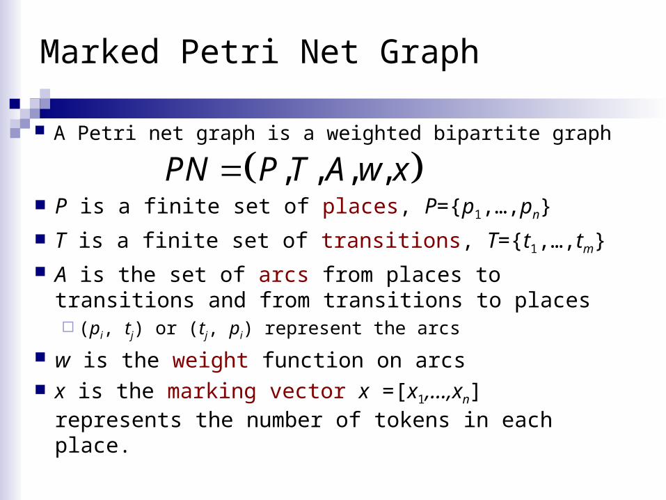
Marked Petri Net Graph

A Petri net graph is a weighted bipartite graph

, , , ,PN P T A w x P is a finite set of places, P={p1,…,pn}

T is a finite set of transitions, T={t1,…,tm}

A is the set of arcs from places to transitions and from transitions to places (pi, tj) or (tj, pi) represent the arcs

w is the weight function on arcs x is the marking vector x =[x1,…,xn] represents the

number of tokens in each place.

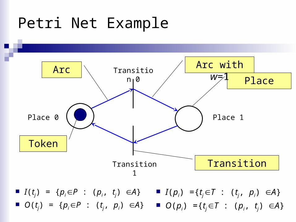
Petri Net Example

Place 0 Place 1

Transition 1

Transition 0

Place

Transition

Arc Arc with w=1

Token

I(tj) = {pi P : (pi, tj) A}

O(tj) = {pi P : (tj, pi) A}

I(pi) ={tj T : (tj, pi) A}

O(pi) ={tj T : (pi, tj) A}

Petri Net Marking

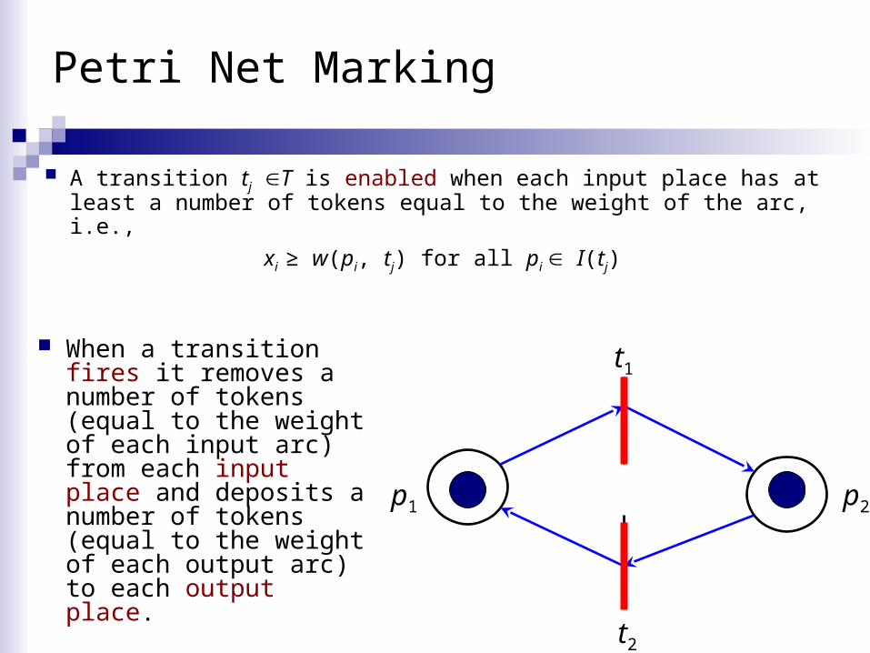
A transition tj T is enabled when each input place has at least a number of tokens equal to the weight of the arc, i.e.,

xi ≥ w(pi, tj) for all pi I(tj)

p1 p2

t2

t1 When a transition fires

it removes a number of tokens (equal to the weight of each input arc) from each input place and deposits a number of tokens (equal to the weight of each output arc) to each output place.

Petri Net Dynamics

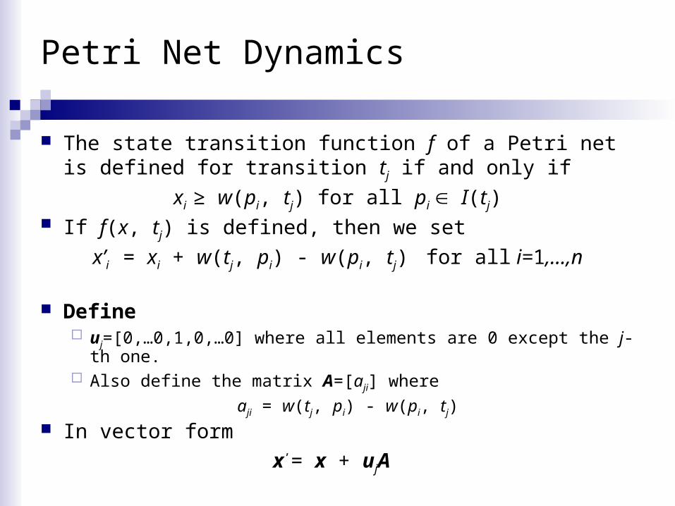
The state transition function f of a Petri net is defined for transition tj if and only if

xi ≥ w(pi, tj) for all pi I(tj) If f(x, tj) is defined, then we set

x’i = xi + w(tj, pi) - w(pi, tj) for all i=1,…,n

Define uj=[0,…0,1,0,…0] where all elements are 0 except the j-th one. Also define the matrix A=[aji] where

aji = w(tj, pi) - w(pi, tj) In vector form

x’= x + ujA

Example: Computer Basic Functions

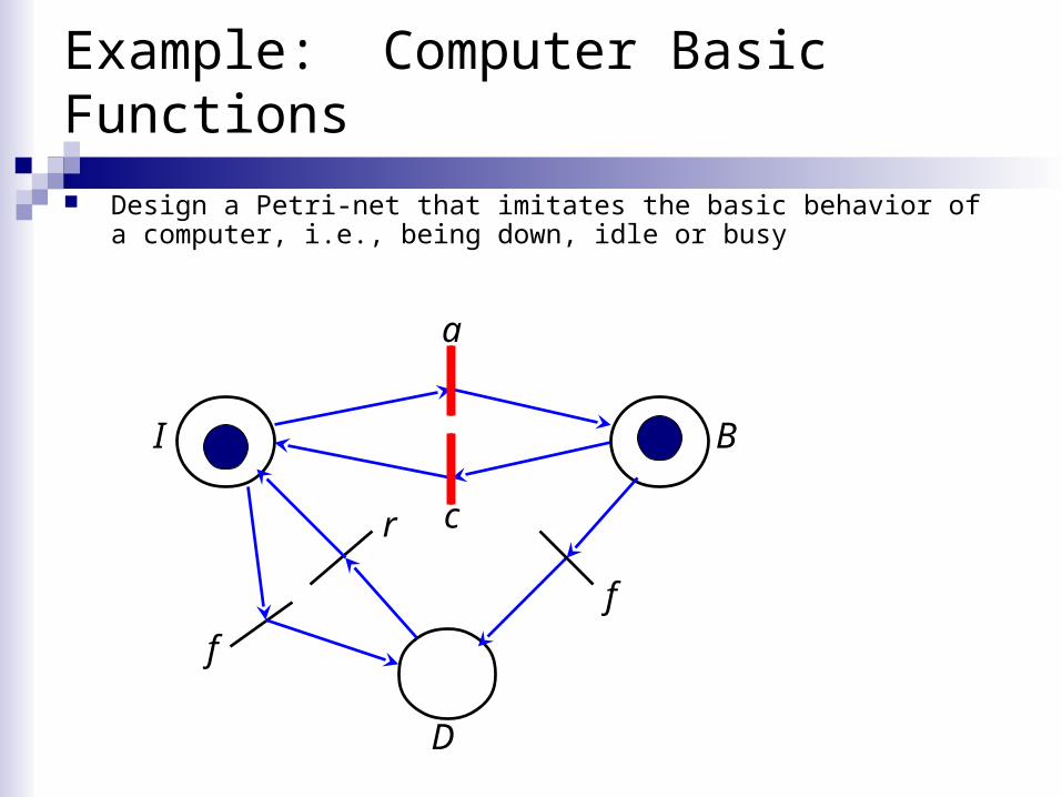
Design a Petri-net that imitates the basic behavior of a computer, i.e., being down, idle or busy

c

D

I B

f

r

a

f

Modeling Protocols Using Petri Nets (Stop and Wait Protocol)

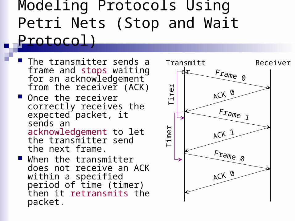
The transmitter sends a frame and stops waiting for an acknowledgement from the receiver (ACK)

Once the receiver correctly receives the expected packet, it sends an acknowledgement to let the transmitter send the next frame.

When the transmitter does not receive an ACK within a specified period of time (timer) then it retransmits the packet.

Tim

erT

imer

Transmitter ReceiverFrame 0

Frame 1

ACK 0

ACK 1

Frame 0

ACK 0

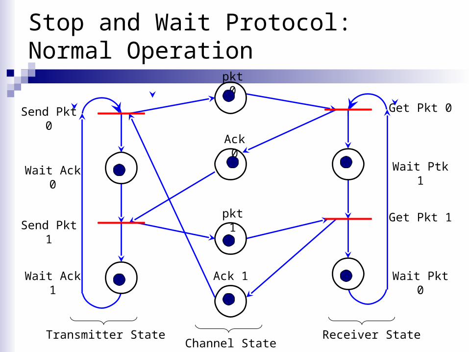
Stop and Wait Protocol: Normal Operation

Wait Ack 0

Wait Ack 1

Wait Ptk 1

Wait Pkt 0

Transmitter State Receiver StateChannel State

Ack 1

pkt 0

Ack 0

pkt 1

Send Pkt 0

Send Pkt 1

Get Pkt 0

Get Pkt 1

Stop and Wait Protocol: Normal Operation

Wait Ack 0

Wait Ack 1

Wait Ptk 1

Wait Pkt 0

Transmitter State Receiver StateChannel State

Ack 1

pkt 0

Ack 0

pkt 1

Send Pkt 0

Send Pkt 1

Get Pkt 0

Get Pkt 1

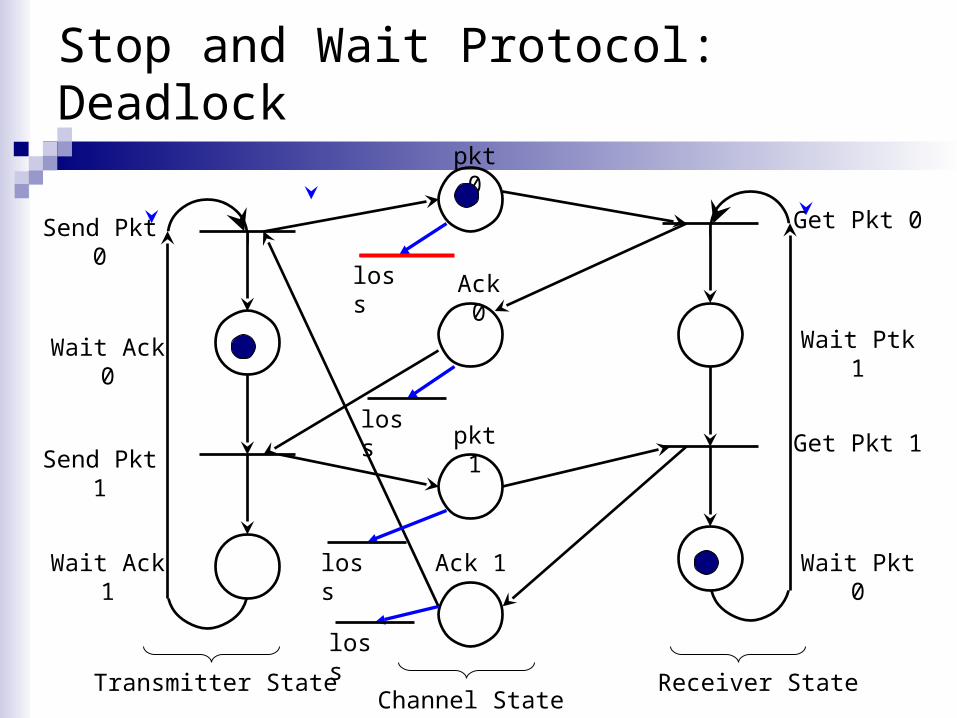
Stop and Wait Protocol: Deadlock

Wait Ack 0

Wait Ack 1

Wait Ptk 1

Wait Pkt 0

Transmitter State Receiver StateChannel State

Ack 1

pkt 0

Ack 0

pkt 1

Send Pkt 0

Send Pkt 1

Get Pkt 0

Get Pkt 1

loss

loss

loss

loss

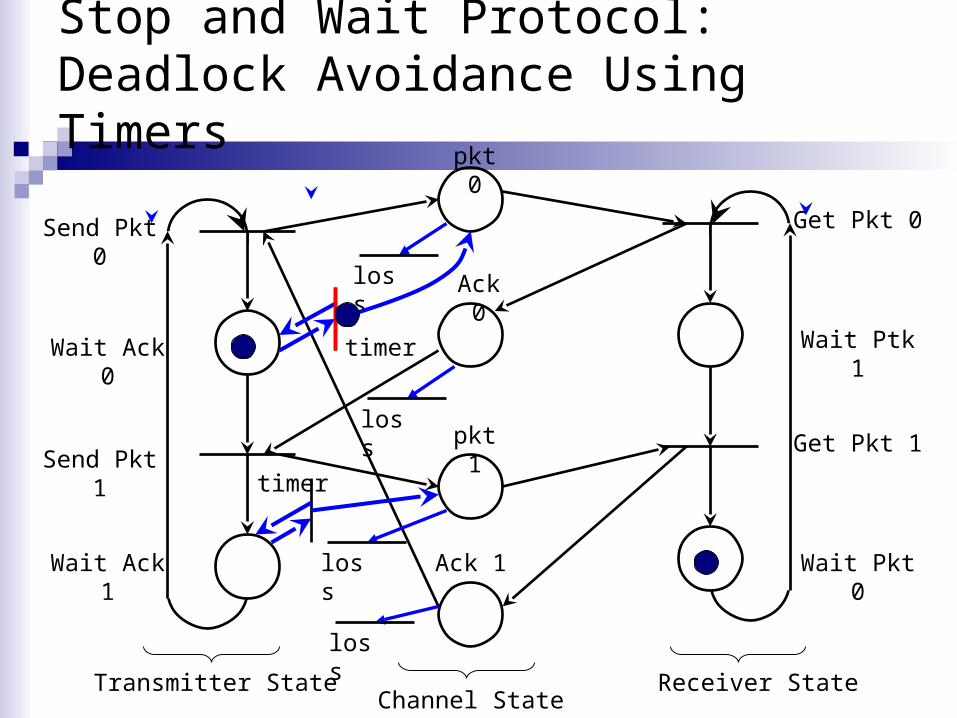
Stop and Wait Protocol: Deadlock Avoidance Using Timers

Wait Ack 0

Wait Ack 1

Wait Ptk 1

Wait Pkt 0

Transmitter State Receiver StateChannel State

Ack 1

pkt 0

Ack 0

pkt 1

Send Pkt 0

Send Pkt 1

Get Pkt 0

Get Pkt 1

loss

loss

loss

loss

timer

timer

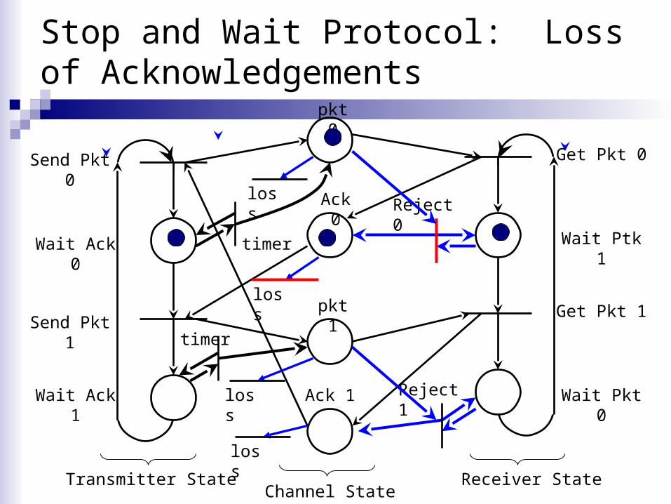
Stop and Wait Protocol: Loss of Acknowledgements

Wait Ack 0

Wait Ack 1

Wait Ptk 1

Wait Pkt 0

Transmitter State Receiver StateChannel State

Ack 1

pkt 0

Ack 0

pkt 1

Send Pkt 0

Send Pkt 1

Get Pkt 0

Get Pkt 1

loss

loss

loss

loss

timer

timer

Reject 0

Reject 1

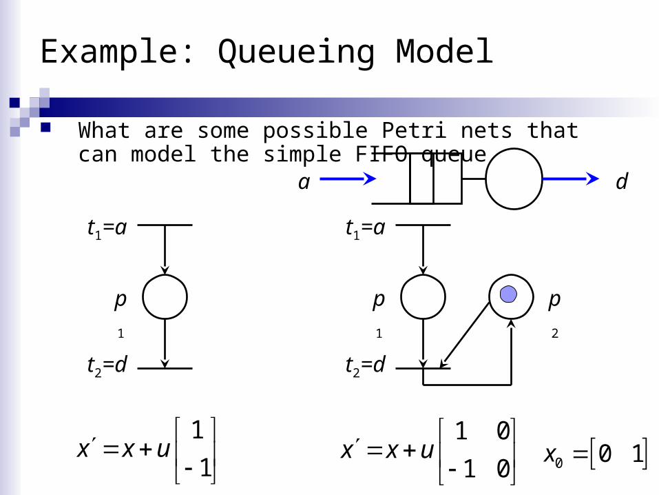
Example: Queueing Model

What are some possible Petri nets that can model the simple FIFO queue

a d

t1=a

p1

t2=d

1

1x x u

t1=a

p1

t2=d

1 0

1 0x x u

p2

0 0 1x

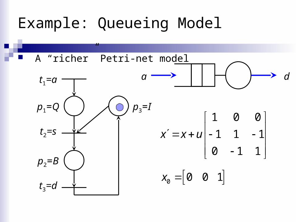
Example: Queueing Model

A “richer” Petri-net model

a dt1=a

p1=Q

t2=s

t3=d

1 0 0

1 1 1

0 1 1

x x u

p3=I

p2=B

0 0 0 1x

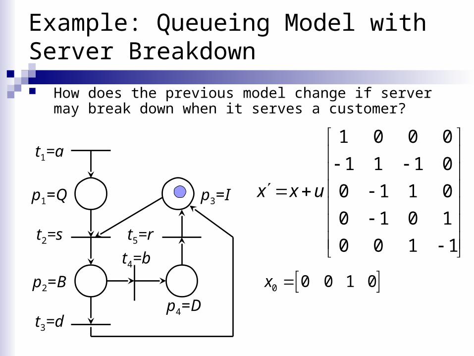
Example: Queueing Model with Server Breakdown

How does the previous model change if server may break down when it serves a customer?

t1=a

p1=Q

t2=s

t3=d

1 0 0 0

1 1 1 0

0 1 1 0

0 1 0 1

0 0 1 1

x x u

p3=I

p2=B 0 0 0 1 0x p4=D

t5=r

t4=b

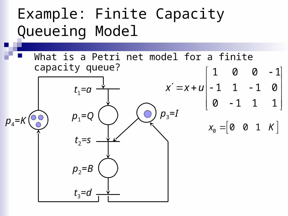
Example: Finite Capacity Queueing Model

What is a Petri net model for a finite capacity queue?

t1=a

p1=Q

t2=s

t3=d

1 0 0 1

1 1 1 0

0 1 1 1

x x u

p3=I

p2=B

0 0 0 1x Kp4=K

Other Petri Net Variations

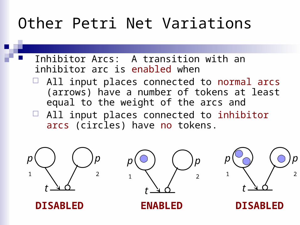
Inhibitor Arcs: A transition with an inhibitor arc is enabled when All input places connected to normal arcs (arrows)

have a number of tokens at least equal to the weight of the arcs and

All input places connected to inhibitor arcs (circles) have no tokens.

p1

t

p2 p1

t

p2p1

t

p2

DISABLED ENABLED DISABLED

Other Petri Net Variations

Colored Petri Nets In this case, tokens have various properties

associated with them. This can be an attribute or an entire data structure. For example, Priority Class Etc.

Timed Petri Net Graph

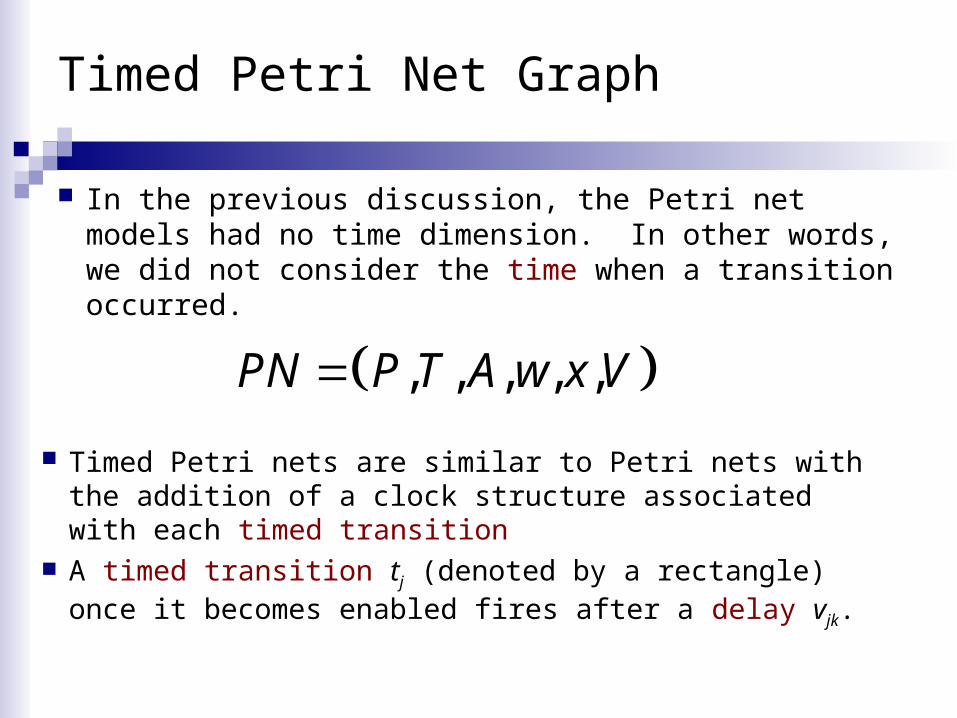
, , , , ,PN P T A w x V

Timed Petri nets are similar to Petri nets with the addition of a clock structure associated with each timed transition

A timed transition tj (denoted by a rectangle) once it becomes enabled fires after a delay vjk.

In the previous discussion, the Petri net models had no time dimension. In other words, we did not consider the time when a transition occurred.

Example: Timed Petri Net

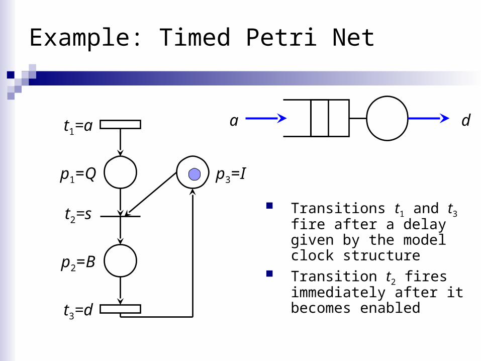
Transitions t1 and t3 fire after a delay given by the model clock structure

Transition t2 fires immediately after it becomes enabled

a d

p1=Q

t2=s

p3=I

p2=B

t1=a

t3=d

Petri Net Timing Dynamics

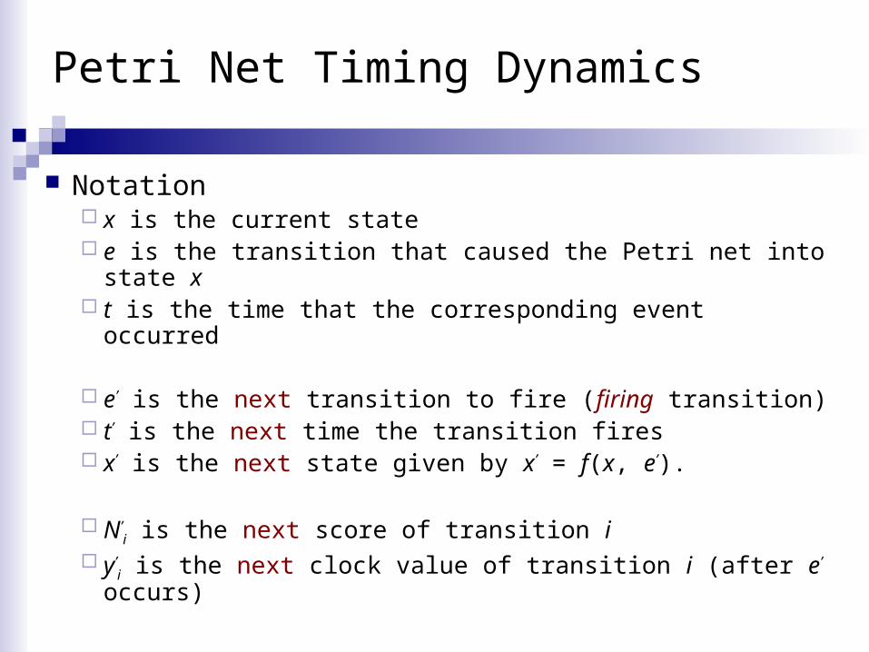
Notation x is the current state e is the transition that caused the Petri net into state x t is the time that the corresponding event occurred

e’ is the next transition to fire (firing transition) t’ is the next time the transition fires x’ is the next state given by x’ = f(x, e’).

N’i is the next score of transition i

y’i is the next clock value of transition i (after e’ occurs)

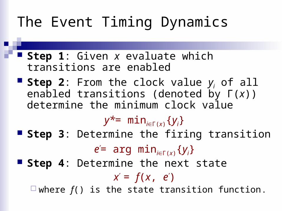
The Event Timing Dynamics

Step 1: Given x evaluate which transitions are enabled

Step 2: From the clock value yi of all enabled transitions (denoted by Γ(x)) determine the minimum clock value

y*= miniΓ(x){yi} Step 3: Determine the firing transition

e’= arg miniΓ(x){yi} Step 4: Determine the next state

x’ = f(x, e’) where f() is the state transition function.

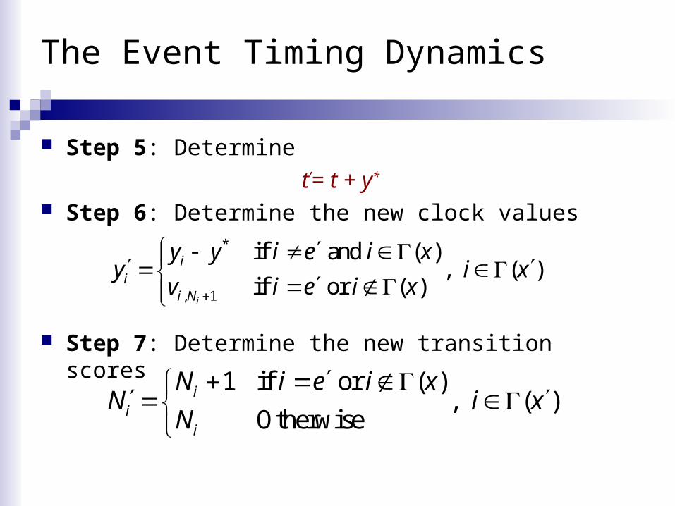
The Event Timing Dynamics

Step 5: Determine

t’= t + y*

Step 6: Determine the new clock values

Step 7: Determine the new transition scores

*

, 1

if and ( ), ( )

if or ( )i

ii

i N

y y i e i xy i x

v i e i x

1 if or ( ), ( )

Otherwisei

ii

N i e i xN i x

N

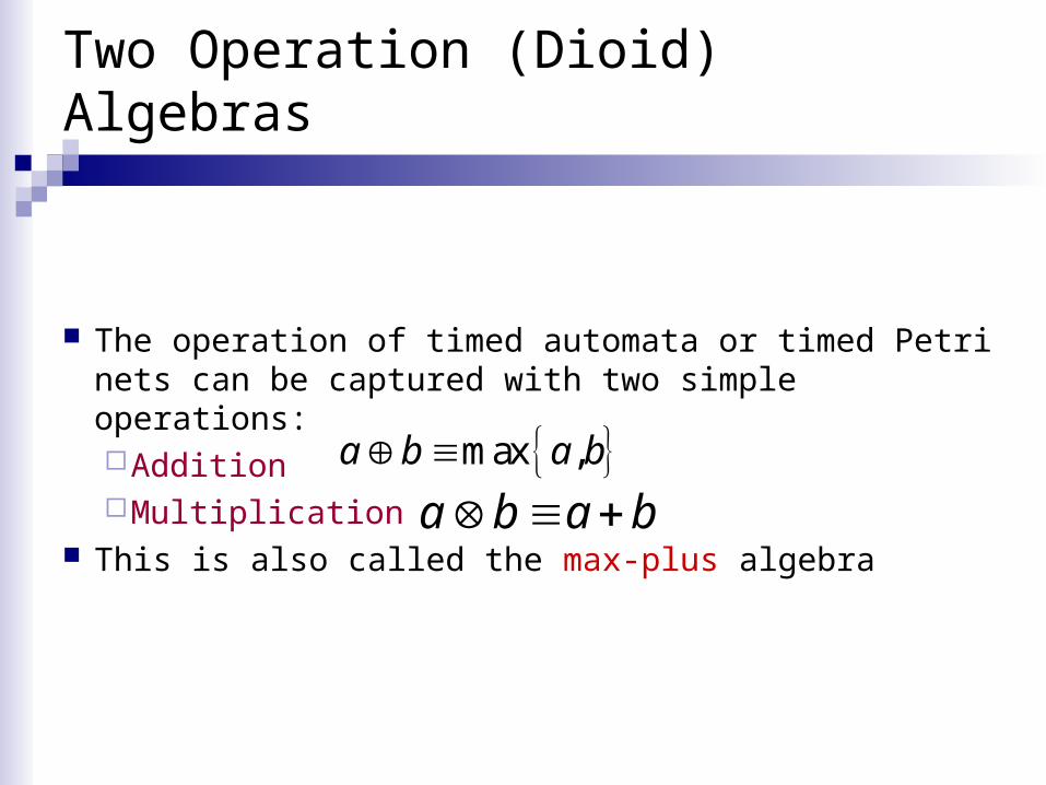
Two Operation (Dioid) Algebras

The operation of timed automata or timed Petri nets can be captured with two simple operations:AdditionMultiplication

This is also called the max-plus algebraa b a b

max ,a b a b

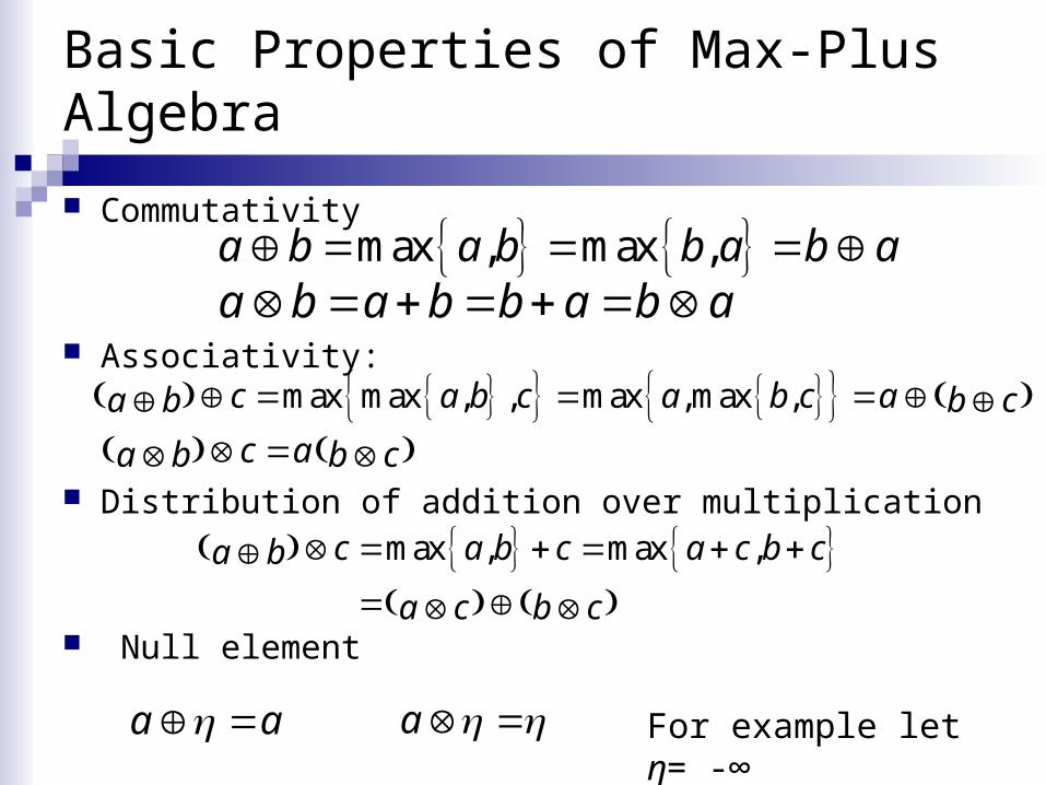
Basic Properties of Max-Plus Algebra

Commutativity

Associativity:

Distribution of addition over multiplication

Null element

max , max ,a b a b b a b a a b a b b a b a

max max , , max ,max ,c a b c a b c aa b b c c aa b b c

max , max ,c a b c a c b ca b

a c b c

a a a For example let η= -∞

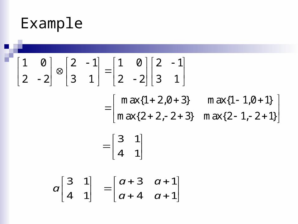
Example

max{1 2,0 3} max{1 1,0 1}

max{2 2, 2 3} max{2 1, 2 1}

1 0 2 1 1 0 2 1

2 2 3 1 2 2 3 1

3 1

4 1

3 1

4 1a

3 1

4 1

a a

a a

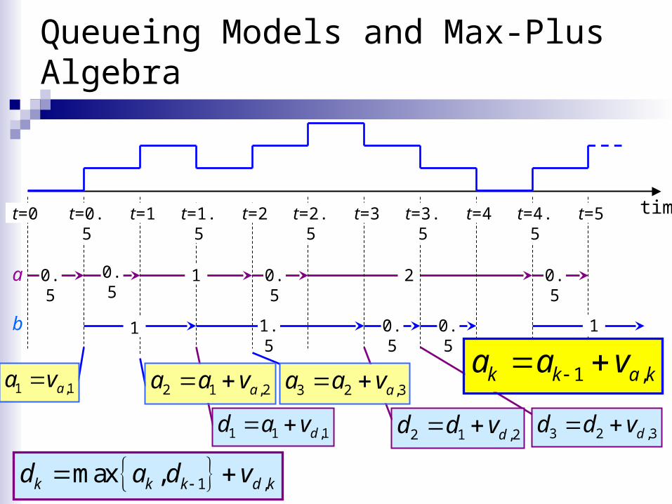
Queueing Models and Max-Plus Algebra

time

a

b

0.5 0.5

1 0.51.5

0.51 2

0.5

0.5

1

t=0 t=0.5 t=1 t=1.5 t=2 t=2.5 t=3 t=3.5 t=4 t=4.5 t=5

1 ,max ,k k k d kd a d v

3 2 ,3dd d v 2 1 ,2dd d v 1 1 ,1dd a v

1 ,k k a ka a v 3 2 ,3aa a v 2 1 ,2aa a v 1 ,1aa v

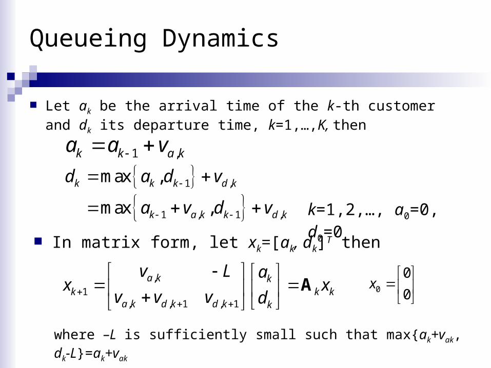
Queueing Dynamics

Let ak be the arrival time of the k-th customer and dk its departure time, k=1,…,K, then

1 ,

1 , 1 ,

max ,

max ,

k k k d k

k a k k d k

d a d v

a v d v

1 ,k k a ka a v

k=1,2,…, a0=0, d0=0

In matrix form, let xk=[ak, dk]T then

,1

, , 1 , 1

a k kk k k

a k d k d k k

v L ax x

v v v d

A 0

0

0x

where –L is sufficiently small such that max{ak+vak, dk-L}=ak+vak

Example

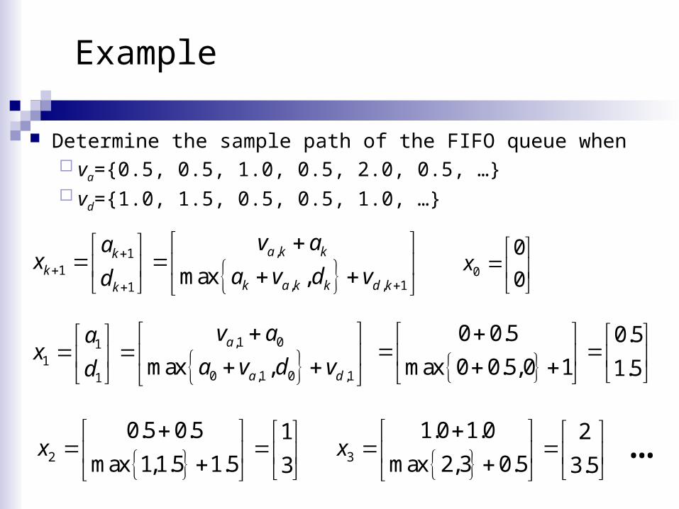
Determine the sample path of the FIFO queue when va={0.5, 0.5, 1.0, 0.5, 2.0, 0.5, …} vd={1.0, 1.5, 0.5, 0.5, 1.0, …}

,1

1, , 11

max ,a k kk

kk a k k d kk

v aax

a v d vd

0

0

0x

,1 01

10 ,1 0 ,11

max ,a

a d

v aax

a v d vd

0 0.5 0.5

max 0 0.5,0 1 1.5

2

0.5 0.5 1

max 1,1.5 1.5 3x

3

1.0 1.0 2

max 2,3 0.5 3.5x

…

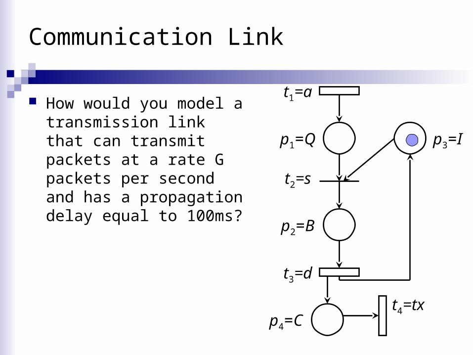
Communication Link

How would you model a transmission link that can transmit packets at a rate G packets per second and has a propagation delay equal to 100ms?

p1=Q

t2=s

p3=I

p2=B

t1=a

t3=d

p4=Ct4=tx