PETREL TIPS Structural Framework

Structural Framework

The Petrel structural framework allows interpretation data to be combined together to construct a

structural model. The structural framework functionality solves many of the problems posed by

complex fault relationships. The model then feeds construction of geocellular models, including stair-

step faults to handle complex geometries. Consequently, these tools improve both the time to model

and the quality of geocellular grids.

The creation of the models can be tightly linked to seismic interpretation, allowing models to be built

on the fly in a "Modeling While Interpreting" workflow. The objective here is to facilitate the creation of

structurally correct interpretation.

Fig 1. To the left, input data like fault interpretations and horizon interpretations. To the right, the

structural framework with faults and horizons.

The principal steps in creating a structural model are contained in three new processes:

Geometry definition, sets up the area of interest.

Fault framework modeling, grids up the faults and creates relationships between connected faults.

Horizon modeling, grids up the horizon data then applies geological rules.

Fig 2. Structural framework with zones.

Corner point gridding is enabled by three processes:

Structural gridding is a new process allowing the generation of a fully stair-stepped corner point grid

directly from the Structural Framework in a single process. This new process is discussed in more

detail in the Structural Gridding topic.

Fault model from structural framework which creates a set of pillar grid faults automatically connected

together and limited to the zone of interest

Stair-step faulting allows the addition of complex faults as IJK stair-step faults.

Fig. 3 The Processes pane with the new Structural framework and Corner point gridding processes in

red frames.

Geometry definition

Fault framework modeling

Fault framework while interpreting

Horizon modeling

Geometry definition

This process is used to define the geometry of the new structural framework by specifying its coverage, defining

the X- Y resolution and optionally the interval in Z (time or depth). The default X and Y coverage and resolution is

automatically adopted from a seismic survey , e.g., the same coverage and orientation as the seismic cube, if this

is available in the project. If multiple cubes are in the project, any cube lattice can be dropped in as a model grid

geometry setting. Other objects that have geometry can also be used, such as horizon and fault interpretation,

point sets and surfaces. The results will vary depending on whether or not the object is defined on a lattice. If it is

not, then the geometry will be set to cover the object with a default rotation and resolution.

A Coarsening factor can be used to create a geometry that honors the input grid extents but with multiples of the

grid increments. In this way seismic trace locations can be honored on the coarse grid. The input geometry can

be set to automatically coarsen, which will target the creation of geometries with less than 60,000 nodes. Petrel

can effectively handle much larger grids but modeling speed can decrease with large grids.

The geometry parameters can be used to edit the coverage by specifying the origin, width, height and rotation of

the lattice. The origin remains stationary when changing the width, height, and rotation. The other two endpoints

cannot be edited and are only shown for reference.

A polygon can be used to create a non-rectangular boundary for the model.

The Z extent of the geometry is normally not user-defined since it adapts to cover surfaces being modeled with

some marginal extension. If desired, this can be overridden with explicit Shallowest and Deepest Z values.

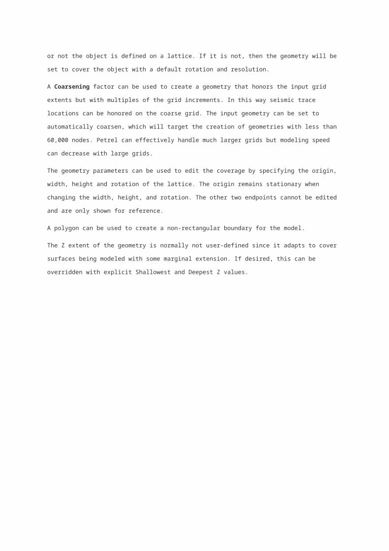
Fig. 1 The Define geometry process dialog

List of Parameters

Parameters and their definitions are listed below.

Parameter FunctionCreate new A new structural framework with the given name will be created.Edit existing

The currently active structural framework will be edited. The framework geometry will change, but any models contained in the framework must be updated by running the relevant processes.

Domain Determines if the structural framework will be in depth or time. It must have the same domain as the interpretation that is going to be used.

Get geometry from selected

Drop objects here and the dialog will attempt to extract a structural framework geometry from it.

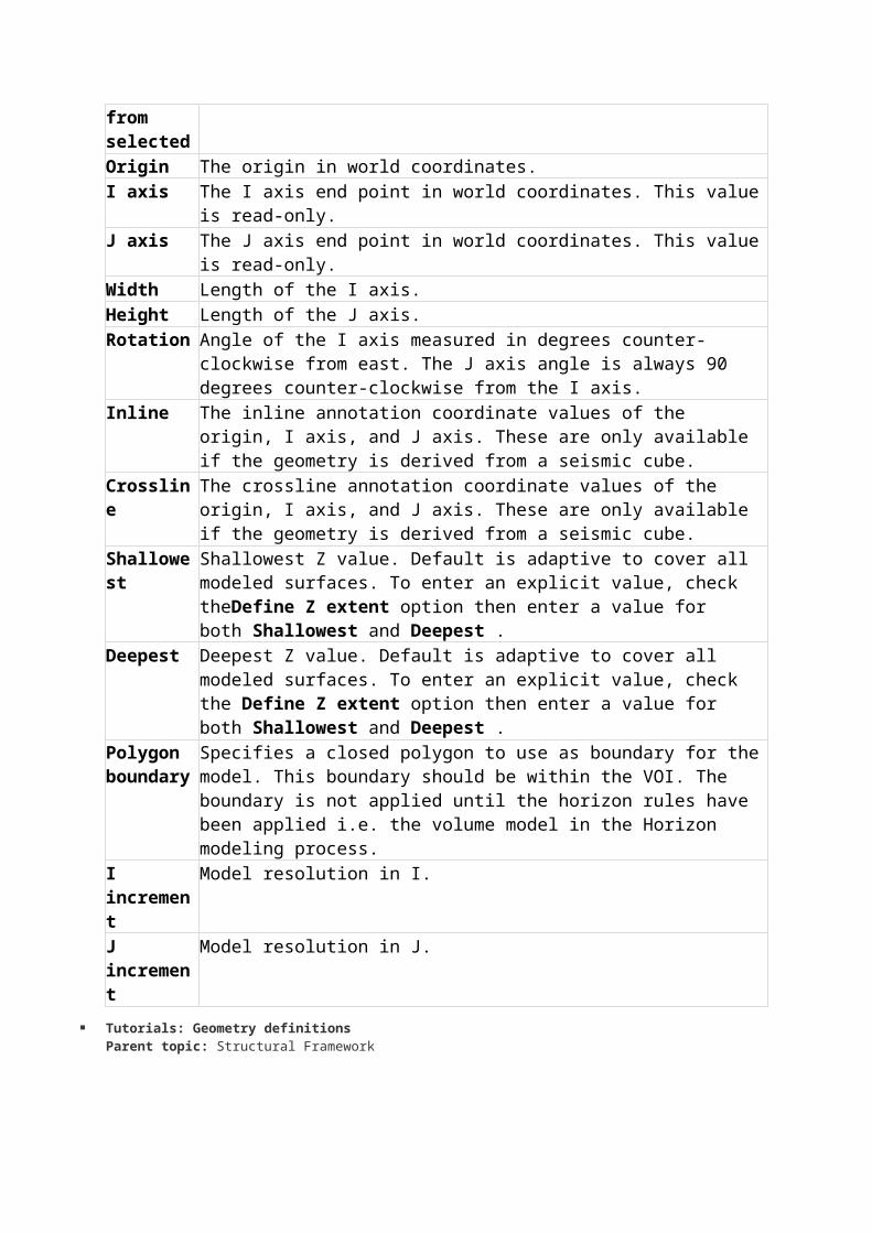
Origin The origin in world coordinates.I axis The I axis end point in world coordinates. This value is read-only.J axis The J axis end point in world coordinates. This value is read-only.Width Length of the I axis.

Height Length of the J axis.Rotation Angle of the I axis measured in degrees counter-clockwise from east. The J axis

angle is always 90 degrees counter-clockwise from the I axis.Inline The inline annotation coordinate values of the origin, I axis, and J axis. These

are only available if the geometry is derived from a seismic cube.Crossline The crossline annotation coordinate values of the origin, I axis, and J axis.

These are only available if the geometry is derived from a seismic cube.Shallowest Shallowest Z value. Default is adaptive to cover all modeled surfaces. To enter

an explicit value, check theDefine Z extent option then enter a value for both Shallowest and Deepest .

Deepest Deepest Z value. Default is adaptive to cover all modeled surfaces. To enter an explicit value, check the Define Z extent option then enter a value for both Shallowest and Deepest .

Polygon boundary

Specifies a closed polygon to use as boundary for the model. This boundary should be within the VOI. The boundary is not applied until the horizon rules have been applied i.e. the volume model in the Horizon modeling process.

I increment Model resolution in I.J increment Model resolution in J.

Tutorials: Geometry definitionsParent topic: Structural Framework

Tutorials: Geometry definitionsHow to define the volume of interest from 3D seismic (or other supported object)

1. In the Processes Pane open the Structural Framework> Define geometry process.

2. Select the 3D seismic to use to define the geometry.

3. Drop it on the blue arrow next to get geometry from selected.

How to define the vertical extent of the volume of interest


2. Check Z extents.

3. Enter Shallowest and Deepest values.

How to define the geometry using origin and angle values


2. Enter

a. Origin

b. Width and Height

c. Rotation

d. I increment and J increment

The values you enter will be automatically updated to ensure orthogonality. The origin is a stationary point. The I

axis endpoint is shifted in the I axis direction so that the extent is evenly divisible by the I increment. Similarly, the

J axis endpoint is shifted, first in the J axis direction so the extent is evenly divisible by the J increment. Then a

rotational shift about the origin is made so that all three points are exactly orthogonal.

How to coarsen the volume of interest (VOI)

When modeling horizons where no salt is present


2. Update the I increment and I increment.

When modeling salt, the model grid geometry mustbe identical to the grid geometry of input

interpretation data.

1. Create a Petrel Surface from your interpretation using the Make/edit surface process. You have full control over

the interpolation options. Define your coarse lattice and interpolate your data. Be sure to select Trend in

the Algorithm tab which is the preferred way to extrapolate salt data (how null interpretations are filled in).


3. Define your geometry using the same exact lattice as the one used in the Make/edit surface process.

4. Switch to the Structural Framework > Horizon modeling process.

5. Use this new Petrel Surface as your data set to model your horizon.Parent topic: Geometry definition

Fault framework modelingFaults are modeled from their inputs into individual smoothed surfaces. Each is bound by a tip loop which

represents the edge of the fault. This tip loop edge is computed from the input fault interpretation with an optional

amount of (user defined) extrapolation which allows each fault to be modeled at or beyond its initial interpretation.

When modeling faults, the Compute faults tab of the process dialog is used, which allows individual settings for

each fault to be modified. Note that the settings can be changed globally for all faults in the Settingstab.

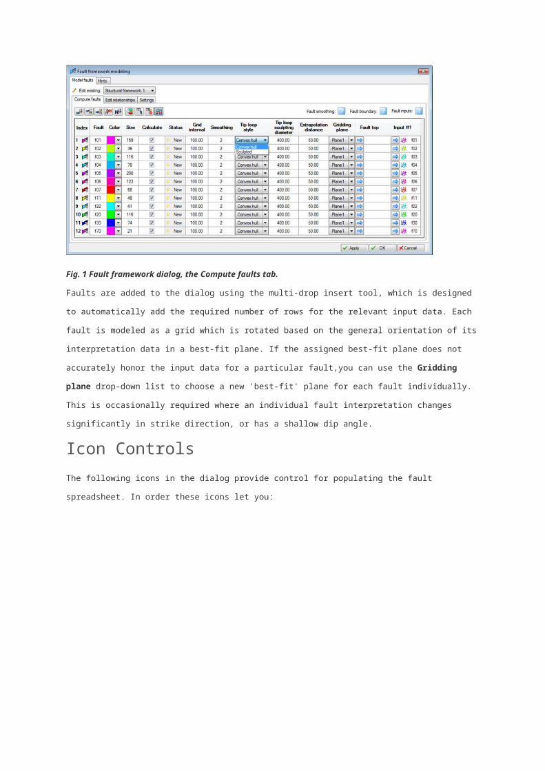
Fig. 1 Fault framework dialog, the Compute faults tab.

Faults are added to the dialog using the multi-drop insert tool, which is designed to automatically add the

required number of rows for the relevant input data. Each fault is modeled as a grid which is rotated based on the

general orientation of its interpretation data in a best-fit plane. If the assigned best-fit plane does not accurately

honor the input data for a particular fault,you can use the Gridding plane drop-down list to choose a new 'best-

fit' plane for each fault individually. This is occasionally required where an individual fault interpretation changes

significantly in strike direction, or has a shallow dip angle.

Icon Controls

The following icons in the dialog provide control for populating the fault spreadsheet. In order these icons let you:

Table Columns: Compute faults tabParameter FunctionIndex IdentifierFault Name of the fault as it will appear in the Faults folder of the corresponding

structural framework.Color Color used to display the faultSize Number of points in all Data Sets defining the fault.Calculate Select the faults to be calculated. By default, all faults are selected.Status The status will be New if not currently built into the model, otherwise, it will

be Done.Grid interval Specifies the resolution of the grid used to create the fault. It should be as high

as possible, while still respecting the data, as this will both speed up the processes and generally results in a cleaner model.

Smoothing Number of smoothing iterations applied. This will generally be used after the Grid interval to fine tune the result. It's better to have a large Grid interval and low Smoothing.

Tip loop style

Tip loops are the boundaries of the faults. There are two alternatives: Convex hull and Sculpted. Convex hull wraps the data with no indents whereas sculpted follows the data more closely.

Tip loop sculpting diameter

Controls the smoothness of a tip loop with sculpted tip loop style. A larger diameter will give a smoother result.

Extrapolation distance

Controls how far beyond the data the fault plane is extrapolated. Not available for sculpted tip loops.

Gridding plane

Faults are gridded in a best fit plane through the data. Normally the automatic selection of the principal plane gives a good result, but in some cases where the fault has a large curvature, you may have to override the default and manually try some different options.

Fault top Fault tops are used to correct the fault plane. The default influence radius is large so a single top will shift the fault plane perpendicular to the gridding plane of the fault. If no other data is present, the Fault tops will be treated as input data.

Input #1 Fault interpretation data used as input data while building the fault. Multiple input columns can be added.

When faults are created, the modeling engine will detect fault relationships and attempt to set a truncation rule

automatically. This is done by assessing the size of faults in a particular relationship, the largest fault is usually

assigned to be the 'Major' fault. All rules are displayed in the Edit relationships tab where they can be edited.

Major (truncating) and minor (truncated) faults can be swapped and the type of the truncation can be changed.

To reverse the truncation of a minor fault, change Above to Below or vice versa. Above or below is in relation to

the major fault and it is difficult to know which side is above and which is below without first applying a rule and

observing the results. Use this binary setting as a way to flip the truncation from what it was previously.

Fig. 2 The Fault framework dialog, the Edit relationship tab

Table columns: Edit relationships tabParameter FunctionFault pair The table lists fault pairs where the major fault is considering truncating the

minor faultVisible Option to visualize or hide the selected fault pairInput Option to visualize or hide the input (fault sticks) for the selected fault pairMajor fault The truncating faultMinor fault The truncated faultTruncation Above/below: determine which side of the major fault the minor fault is

truncated

Remove truncation: set to no truncation

Swap major-minor: change around the fault pair, i.e. swap major and minor

faults

Force truncation calculation: reapply the Petrel fault relationship logic to the

chosen fault pair.Verified Reminds the user that the relationship has been verified. Verifying has no effect

on the modelRecalculate all relationships

reapply the Petrel fault relationship logic to all fault pair

Editing of fault truncation relationships can also be carried out in the 3D window using the right mouse button

context-sensitive menu. This allows users to:

Display input data of the fault framework.

Show connected faults.

Alter fault extrapolation distance.

Swap major/minor fault truncation relationships.

Swap minor fault above/below truncation.

Remove minor fault truncation.

Remove all truncations on a fault.

Force (Auto calculate) fault truncation relationship between two faults.

Altering the Major/Minor Fault truncation relationships in the 3D window is achieved by selecting a fault pair. This

is done by initially activating one fault and then selecting (using the right mouse button) the other fault in the

desired pair. This action defined the fault pair that the operation will be carried out on. Once the fault pair is

selected, you may alter the relationship between them by swapping relationships. The image below outlines this

process where a major fault is highlighted (bold line highlighting the fault tip-loop) and then each fault truncation

can be altered, removed or recalculated by right clicking on each minor fault respectively.

Fig. 3 Fault context menu in 3D window

Fault grids are typically small in size and do not consume much memory or require much computation when

compared with horizon modeling. It is however good practice to have as large a grid interval as can be supported

while still honoring the input data.

Getting the fault relationships correct in a structural model is a critical first step. Accurate geologically sound fault

models will save time later in the workflow. It is very common that problems arising during horizon modeling are

due to faults not being correctly modeled and intersected.

Some tips to consider are:

Does the fault interpretation make good geological sense? Is this structurally feasible?

Does each minor fault have a solid intersection with its major fault? Does this fault-fault intersection continue

deeper into the earth model where it should? If this intersection breaks down with depth, horizons modeled at

those levels will show the two faults disconnected (not bifurcated). This may be okay if it reflects reality.

Are faults modeled to their true X,Y and Z extent within the model VOI? Sometimes faults are not fully

interpreted, leading to faults not modeled deep or shallow enough. Incomplete fault models can lead to degraded

horizon models.

Do faults extend beyond where they truly exist? Make sure any extrapolation is reasonable.

Starting out it is prudent to consider excluding some of your faults. For the ones you do model, make sure they

honor the input data and make geological sense. Often, it adds to overall modeling efficiency to start out with the

more important faults (the ones with large vertical throw) and subsequently add subordinate faults (usually ones

with smaller throw). Quite often, this method will expose many issues that will adversely affect horizon modeling

results. This can also give you a better understanding of how the workflow reacts to updating your model with

additional faults.

Fig. 4 Fault framework dialog, the Settings tab

Parameters FunctionGrid interval This controls the faults grid interval. It should normally be gridded with a

coarser interval then the horizons.Smoothing This controls the overall smoothness of fit to fault data expressed as the number

of smoothing passes. Set 0 for no smoothing and higher numbers of passes for increased smoothing.

Tip loop style

This controls the general shape of the tip loop.

Convex hull

SculptedTip loop sculpting diameter

This control varies the degree to which the tip loop is sculpted or shrink wrapped to fit the data. Only applied when the tip loop style is set to Sculpted. A small diameter results in more sculpting, while a large diameter results in less sculpting. An extremely large diameter produces a convex hull fit to the data. The effect is like a ball rolling around the edge of the data where a small diameter enables the ball to roll between data points with at least this distance of separation.

Extrapolation distance

This horizontal distance controls the distance the tip loop is extrapolated beyond the data.

Fault top influence radius

Controls how far a well top correction is spread out from the top. The correction is applied in the best fit plane of the fault. A large correction distance (default) will essentially move the fault perpendicular to the best fit plane.

Apply to all faults

This applies the selected settings to all faults.

Tutorial: Fault modelingParent topic: Structural Framework

Rate this listing

Tutorial: Fault modelingHow to model faults

1. In the Processes pane, open the Structural Framework > Fault framework modeling process.

2. Select the model you want to build/edit as the Active model

3. Select the Faults tab.

4. Inspect your faults and update the relevant information.

5. Build your Structural Framework by clicking either OK or Apply

How to model one fault with multiple data sets

1. In the Processes pane open the Structural Framework > Fault framework modeling process.



4. Click the Append a column in the table button . A new Data Set column is added at the end of the table.

5. Select your data in the Petrel Input tree and drop them in the new Data Set column for the appropriate fault.

6. Build your Structural Framework by clicking either OK or Apply

How to drop data for multiple faults

1. In the Processes Pane open the Structural Framework > Fault framework modeling process.



4. Click the Enable/disable multiple drop in the table button .

5. Add the appropriate number of rows in the table, one for each fault. Click the Set number of items in the table button , enter the number

of faults and click OK

6. In the Petrel Input pane, select the first fault interpretation to be dropped.

7. In the Faults tab, select where this first fault should be dropped. That fault and other subsequent ones will be populated with their

respective interpretation data.

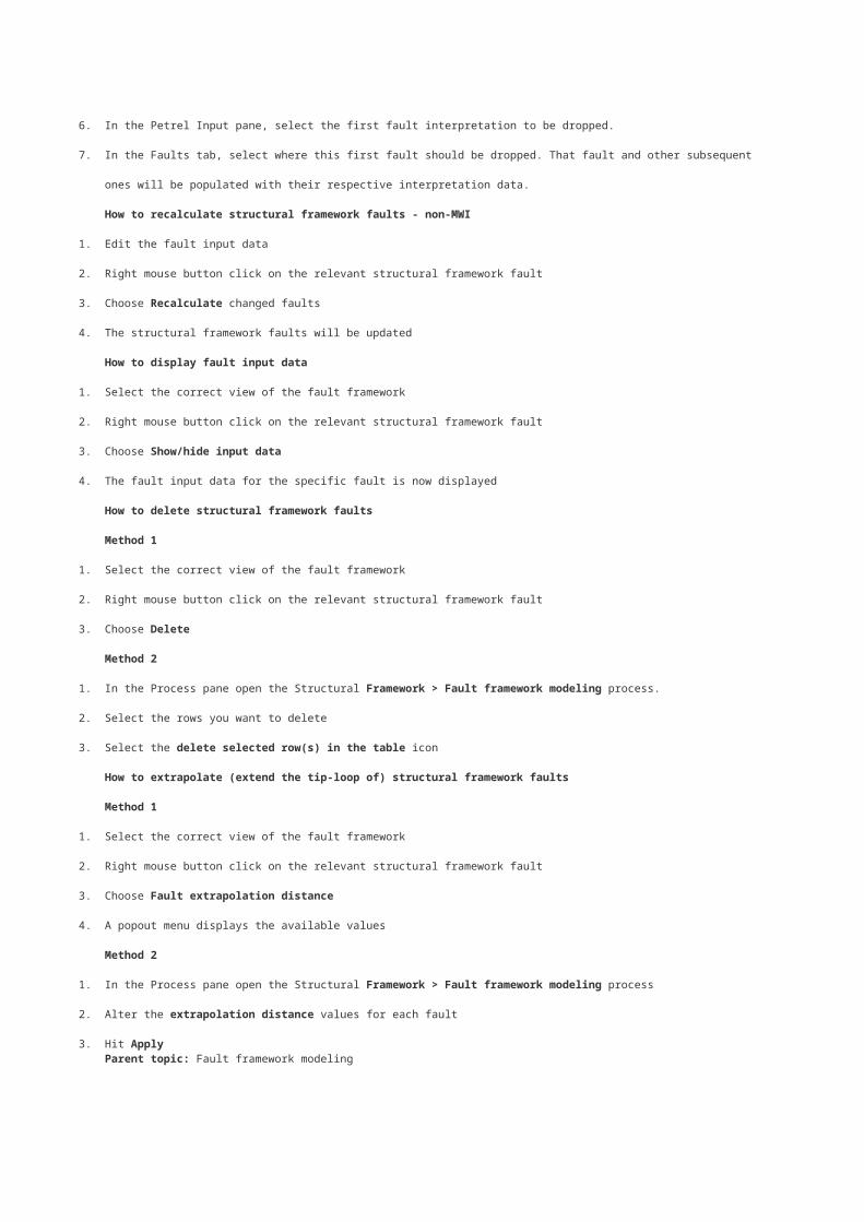
How to recalculate structural framework faults - non-MWI

1. Edit the fault input data

2. Right mouse button click on the relevant structural framework fault

3. Choose Recalculate changed faults

4. The structural framework faults will be updated

How to display fault input data

1. Select the correct view of the fault framework


3. Choose Show/hide input data

4. The fault input data for the specific fault is now displayed

How to delete structural framework faults

Method 1



3. Choose Delete

Method 2

1. In the Process pane open the Structural Framework > Fault framework modeling process.

2. Select the rows you want to delete

3. Select the delete selected row(s) in the table icon

How to extrapolate (extend the tip-loop of) structural framework faults

Method 1



3. Choose Fault extrapolation distance

4. A popout menu displays the available values

Method 2

1. In the Process pane open the Structural Framework > Fault framework modeling process

2. Alter the extrapolation distance values for each fault

3. Hit ApplyParent topic: Fault framework modeling

Fault framework while interpretingPetrel Structural framework delivers new functionality which allows rapid real-time creation of the structural framework during fault and

horizon interpretation and update of the framework by editing geophysical interpretation. Fault model from structural framework places

geophysical interpretation at the core of good model building by fully integrating with the seismic interpretation tool set. This allows

users to

Get it right the first time - Asset teams fix modeling problems in the context of seismic data.

Direct link between geophysical interpretation and geocellular modeling.

'On the fly' approach to fault relationships, horizons and model construction.

Improved QC speed and functionality.

Quick validation of varied seismic interpretation within the 'Petrel Unified Environment'.

Often geophysical interpretations are incompatible with geocellular modeling constraints and subsequently, due to modeling limitations,

interpretation needs to be edited to build a coherent geocellular model. This often happens without any reference to the original seismic.

Fault framework while interpreting fully-integrates geophysical interpretation as part of the core structural framework construction

process. Faults are automatically added to the fault framework as interpretation progresses and critical fault-fault relationships can be

interactively constructed at the time of interpretation. This verifies the fault-fault relationships by the geophysicist and removes the need

for later editing by geologists/modelers. During fault interpretation, the faults are gridded and intersected "on the fly" as new data is

added or changed. Horizons are gridded or re-gridded on demand as the interpretation is modified.

Fig 1. The "right mouse button" -menu on a fault interpretation folder.

How to use Fault framework while interpreting

Display preferred interpretation environment (3D/2D Interpretation window).

Display Seismic Data (2D/3D).

Insert New Interpretation Folder.

Insert a new fault in interpretation folder (use RMB context menu or interpretation manager).

Right click on the new interpretation folder and choose 'Fault framework while interpreting.

Use the Fault interpretation tool from Seismic Interpretation and start interpreting the fault in the 3D or 2D Interpretation window.

Fig 2. Fault framework while interpreting in a 3D window while displaying a time-slize and a cross-line.

'On-the-fly' computation of Fault-Fault Intersections

Parent topic: Structural Framework

Horizon modelingOnce the fault framework is completed, adding horizons is the next key workflow. Given horizon data, geologic relationships and

modeling parameters, the Horizon modeling process will first create horizons individually honoring the fault surfaces, and then apply

horizon truncation rules. Results are stored in the Petrel Models tab as collections ofHorizons and Zones under the named Structural

frameworks.

Along with interpretation data other kinds of input data can be used to model horizons.

Well tops are used to tie horizons to interpreted well points. Influence radius around well tops along with other horizon adjustment

settings are defined in Settings tab. Well tops, or any sparse data, can also be used without any other inputs using the conformal

modeling option.

Hard data is usually used to guide horizons along the fault surfaces or in thin fault blocks. It is really no different from any other input

data except that it is not filtered close to the faults.

Isochore is a zone thickness map. It can be used for a better pinch-out handling and control over the zone volumes. Isochores stack up

or down from the reference horizon when conformal modeling is chosen. If the isochores have a zero thickness area, then this should

be extrapolated to be negative to ensure clean horizon intersection lines.

Input field is a general input field for seismic interpretation, points or surfaces. Extra input columns can be added to accommodate

multiple inputs, this is often necessary for multi-Z inputs such as reverse faults. The data provided in the input field will be filtered out

around the faults.

Fig. 1 Horizon modeling dialog, the Compute horizons tab.

Horizons must be entered in their correct stratigraphic order. A typical layer-cake stratigraphy is the default option (Conformable),

unconformities, disconformities and salt interfaces must be designated so that horizon intersections are correctly modeled.

If surfaces intersect they are truncated according to their type (Horizon type option). Available types are listed in the table columns

below: The different Horizon type settings are applied by selecting the option "Apply geological rules and create zone model" in the

dialog window.

Fig. 2 Horizons are trimmed according to their type

When rules are applied to surfaces they are applied in correct stratigraphic surface order, e.g., starting with the oldest surface and

finishing with the youngest surface.

Surfaces with only sparse data may be guided by another surface, this is conformal modeling. Use the Conforms To column to select

another surface. The horizon will be shaped by that surface. This is done by first computing an isochore, then stacking that isochore

onto the reference (conformal) horizon to produce the final horizon model. When modeling all horizons, any horizon declared as a

conformal reference to another horizon is modeled first and then the conformal horizon is modeled.

Table Columns: Compute horizons -tab

ParameterFunctionIndex Index for horizons used for "Conform to" settingsHorizon Horizon name, automatically picked up from the Input #1 column. Names can be

edited in the Horizon column. Horizon names will appear in the Horizons folder of the corresponding structural framework.

Color Color used to display the horizon in Petrel windows.Calculate Select the horizons to be calculated. By default, all horizons are selected.Status The status will be New if not currently built into the model, otherwise, it will

be Done .Horizon type

Depositional - a sedimentary horizon usually 'moulded' by adjacent depositional

horizons. Where two depositional horizons meet, the younger is truncated to

onlap the older.

Erosional - unconformity which truncates older horizons. Parts of an older

horizon above the erosional surface are truncated. Younger horizons are ignored.

Base - unconformity which truncates younger horizons. Parts of a younger

horizon below the base surface are truncated. Older horizons are ignored.

Discontinuity - unconformity which truncates younger and older horizons (a

combination of erosion and base types). Younger horizons crossing a

discontinuity are truncated below the discontinuity; older horizons crossing a

discontinuity are truncated above the discontinuity. Truncations apply regardless

of surface type. Where two discontinuities meet, the younger is truncated to the

older.

Salt Top - a salt surface representing one or more local tops of salt.

Salt Base - a salt surface representing one or more local bases of salt.

Salt Cap - a salt surface representing one or more tops of salt where edges are

modeled vertically down from the cap. The salt base is either the VOI base or

another Salt Base surface if that surface is the next oldest in the table.

Salt Body - a triangulated mesh surface representing one or more salt bodies.

A Salt Body surface has already been modeled, whereas all other surface types

are internally modeled by the Structural framework dialog.Conforms to

Select a horizon this horizon conforms to:

None

Another horizonSmoothing

Number of smoothing iterations applied.

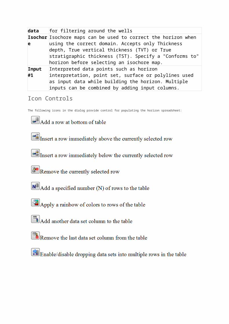
Well tops Well tops are used to correct the horizon as a post processing step.Hard data No different to other data except it is not subject for filtering around the wellsIsochore Isochore maps can be used to correct the horizon when using the correct domain.

Accepts only Thickness depth, True vertical thickness (TVT) or True stratigraphic thickness (TST). Specify a "Conforms to" horizon before selecting an isochore map.

Input #1 Interpreted data points such as horizon interpretation, point set, surface or polylines used as input data while building the horizon. Multiple inputs can be combined by adding input columns.

Icon Controls

The following icons in the dialog provide control for populating the horizon spreadsheet:

Fig. 4 Horizon modeling dialog, the Common settings tab.

List of parameters: Common settings tab

Parameter Function

Well adjustmentInfluence radius If the influence radius is not specified, the radius is set to infinity.

Petrel will calculate a residual surface (difference between the horizon before and after correction).

Correct at all cells penetrated by well accurate

Well report Iconize the residual surface

Iconize the residual points

Horizon Modelling QC OutputUnfaulted smooth surface

Creates an smoothed unfaulted surface from the horizon input data to identify the fault centreline location, this surface can be controlled using the coarsening and z-offset options under other settings

All points used (points outside the fault influence)

This creates two point sets which highlight the input data which was used to create the horizon in the structural framework and the data which was filtered away (around faults) based on the 'distance to fault' settings

Fault center lines Creates a polyline set of the intersection between the unfaulted smooth surface and faults in the structural framework

Problem locations Creates a point set which attempts to identify where problem locations are in the modelled structural framework horizon.

Other settingsCoarsening factor for the unfaulted horizon

The unfaulted grid is used to calculate the fault midline. The increment (grid cell size) of the initial unfaulted grid will be the (coarsening factor * increment) greater than the increment defined in the Geometry definition process. Recommended values are 1 to 5, where 1 is the same as the increment defined in the Geometry definition process.

Z offset of the unfaulted horizon

The horizon modeling process must first detect faults by intersecting a smooth surface with the faults for creating a initial centerline. The surface and resulting center lines can be viewed by using the iconize option.

Compute horizons in rectangular area defined by polygon

Polygon for temporarily reducing the area for horizon calculating.

Salt modeling technique

Clamshell salt modeling technique : Cause a zone to be created by fully extrapolating the salt surfaces to the extent of the model and then truncating the extrapolated surfaces against each other. All parts of the extrapolated Salt base which are above the Salt top will be deactivated, similarly, all parts of the extrapolated Salt top which are below Salt base will be deactivated. For a simple pair of top and base, this can be resemble to halves of a clam when closed, hence the name. Multiple top and base pairs can be used to model complex salt overhangs. All salt zub regions are merged into one single salt zone. Complex clamshell salt modeling technique : This option does no

extrapolation. It requires the input surfaces or interpretations to be modeled on the same grid as in the Geometry definition. Sparse interpretations are not recommended as the can result in very strange models containing empty columns. Each top and base pairs are filtered to ensure they are corresponding samples in both top and base. The surfaces are then truncated each other where they are defined by the same rule: deactivate base above top and deactivate top below base.

With horizons identified as Salt Top and Salt Base, there are two Salt modeling technique options in the Horizon modeling Common

settings tab: Clamshell and Complex Clamshell. These techniques merge all salt sub-regions into a single salt zone.

The Clamshell option will cause a salt zone to be created by fully extrapolating the salt surfaces to the extent of the model and then

truncating the extrapolated surfaces against each other. All parts of the extrapolated Salt base which are above the Salt top will be

deactivated; similarly, all parts of the extrapolated Salt top which are below the Salt base will be deactivated. For a simple pair of top

and base, this can resemble two halves of a clam when closed, hence the name. Multiple top & base pairs can be used to model

complex salt overhangs. All salt sub-regions are merged into a single salt zone.

The Complex Clamshell option does no extrapolation. It requires the input surfaces or interpretations to be modeled on the same grid

as the Define geometry grid. Sparse interpretations are not recommended as they can result in very strange models containing empty

columns. Each top and base pair is filtered to ensure there are corresponding samples in both the top and base. The surfaces are then

truncated against each other where they are defined with the same rule: deactivate base above top and deactivate top below base. This

approach helps remove bubbles. The precise filtering rules are as follows:

If a top pick is located above its corresponding base pick, then this salt interval will be considered valid and will be kept as it is.

If a top pick is located below its corresponding base pick, then this salt interval will be considered invalid and will be ignored. Basically,

the top pick is snapped onto its corresponding base.

If there are Interleaved top/base configuration and both salt intervals are considered valid, then the lowest top is dropped onto the

highest top and the highest base is dropped onto the lowest base.

If a top pick is determined to be a single top interpretation (no corresponding base), then a corresponding base will be created at the

base altitude of the volume of interest and from that point will be processed as any other top/base pair.

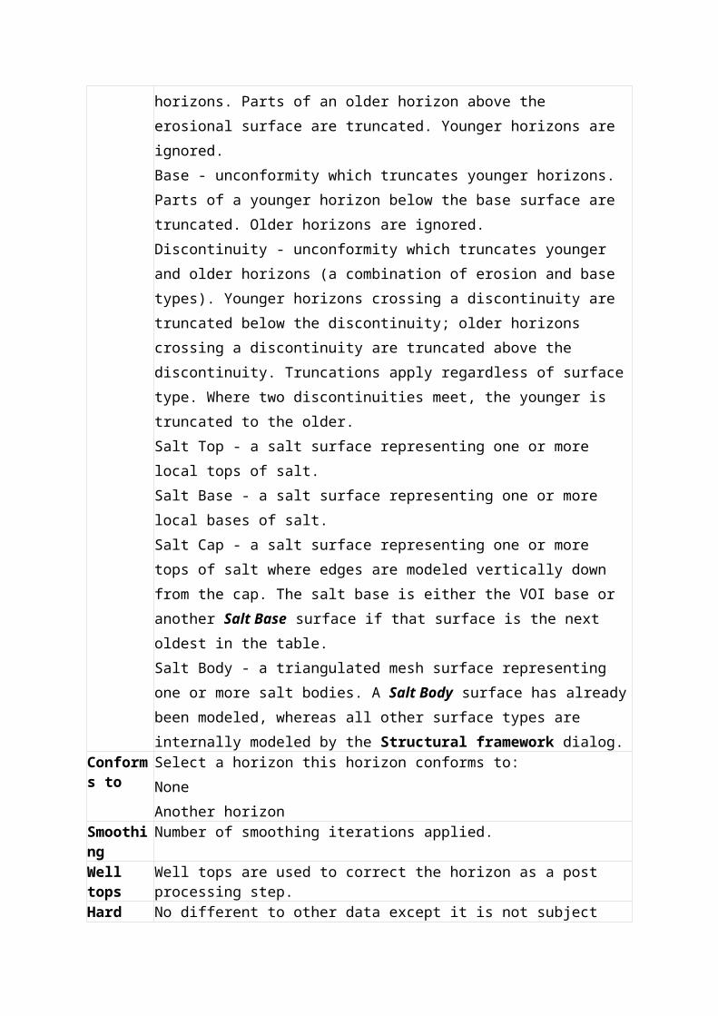
Fig. 5 Horizon modeling dialog, the Fault settings tab.

List of parameters: Fault settings tab

Parameter FunctionUse default Petrel will use default settings when this position is selected. Must be

deactivated for using other settings.Active fault If not active the faults will have no displacement for the horizonsDistance to fault

Input data that are closer than this distance (measured horizontally) to the fault are treated as uncertain and are not used in the interpolation algorithm. Petrel will then back-extrapolate into the fault plane.

Per side The extrapolation distances can be specified differently for the front and back sides of the fault. By using this selection, the different sides will be marked in the 3D window.

DisplacementMin/Max The fault displacement will be modeled from the input data as normal, but

where the offset is less than the minimum or greater than the maximum, it will be changed. For constant offset on the entire fault, simply set the minimum equal to the maximum. The displacement is measured vertically.

Allow hinge Allows faults to swap between reverse and normal displacement along its length. With this option selected, Petrel will create the offset according to the input data and then decide which side of the fault is downthrown.

Smoothing Smooth the fault displacement. Select this option to access the Number of iterations and/or Tolerance settings. Displacement smoothing is recommended, and should be used if min or max displacement is specified.

Number of iterations

Set number of smoothing iterations. Recommended values are 3-10.

Tolerance Make a smooth displacement with a maximum change (tolerance) pr. 100 horizontal units along the fault.

Horizon modeling tips

It is often more efficient to model horizon by horizon using the Calculate option to turn on/off individual horizon calculation.

It is good practice to first build horizons without applying horizon rules. It saves time but also allows control of horizon-horizon

intersections before they are clipped.

If a conformably modeled horizon is unacceptable, then choose the settings option Iconize all points used, this will produce a point set

which represents the input created by the system. Now use this directly in the Horizon modeling table to enable editing of the input data.

Use the fault center lines. Iconize the fault center lines when running the horizon modeling. Each fault will be split with a different color

at intersections. It is usually a good idea to study the center lines in the 2D window to find problem areas. Once a problem is identified,

observing the center lines in 3D, together with the faults and their intersections, will help find a solution to the issue.

Control the filtered data. Iconize filtered data to identify wrong sided data.

Adjust fault filtering. Filter distance can be adjusted on a fault by fault, horizon by horizon basis in the faults tab of horizon modeling.

However it is good practice to keep a small blanking distance and erase wrong sided data instead.

For faults that are not active, use the faults tab to disable them for a given horizon.

Fig 8. The Fault settings tab in the Horizon modeling process. The fault F3 is deactivated by deselcting the Active fault option.

Use local area calculations. To improve speed of interactive horizon work, set a temporary boundary in the area of interest.

Fig 9. The option Compute horizons in rectangular local area defined by polygon for performing local area calculations. This

option is located in the Common settings tab in the Horizon modeling process.

Apply Geological rules and create Zone Model

Horizon modeling can be split into two stages, initial horizon generation for QC and the final modeling stage, where correct geological

rules are applied to each model horizon. Applying correct geological rules ensures all model horizons are ordered and cut correctly and

knits each horizon to fault surfaces. This process creates a model with zones.

This option is toggled in the Horizon Modeling process and can be independently run from the horizons. Once all horizons have been

generated and have undergone QC, theCalculate checkboxes for each horizon row can be deselected. Toggle on the Apply

Geological Rules & Create Zone Model to finalize the rules on each model horizon.

You may choose to turn this option on as default, however once applied there is no option to see the intermediate horizon modeling

results and QC processes may prove difficult.

Fig 10. Initial Horizon modeling step prior to application of geological rules

Fig 11. Geological rules applied - all horizons now correctly eroded by top surface

Fig 12. Generated Zone model

Visualize a Structural Framework

All components of a Structural Framework (Horizons, Faults or Zones) are represented as triangle meshes. Their level of detail can be

adjusted to render only a fraction of the model.

Horizon modeling can create discontinuous meshes constituted of patches. You can visualize those patches independently using

random coloring. Some patches, referred to as unreal patches, were discarded during the modeling process, however, they can be

visualized for trouble shooting.

Free framework model memory

Large structural frameworks can occupy a lot of memory. The Free framework model memory frees all significant memory of a

structural framework, and is recommended if users want to work with more than one structural framework. This prevent keeping multiple

large models in memory.

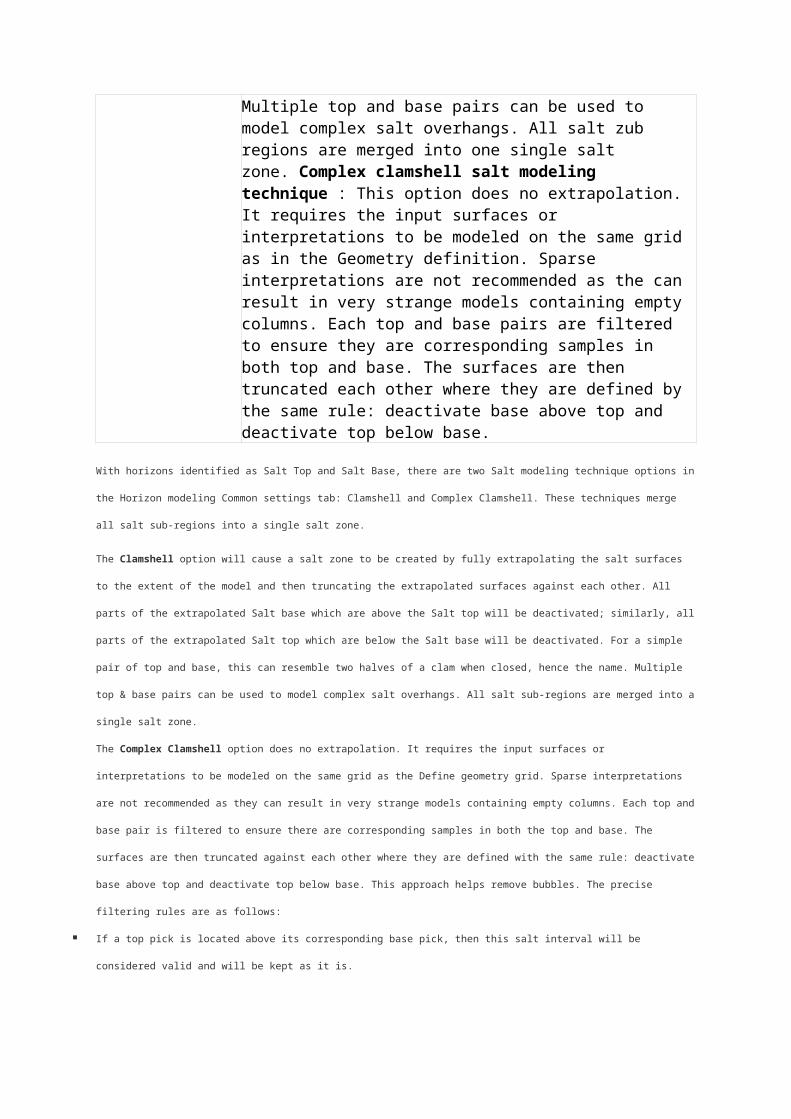
Fig 13. The Free framework model memory"option available from the Tools menu.

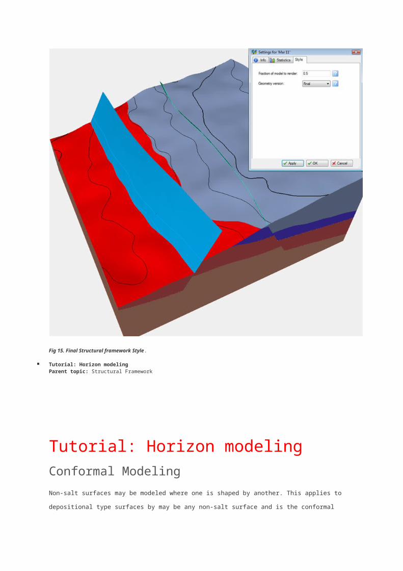
Initial vs Final Visualization

Once the application of geological rules has been carried out, you are able to toggle between the initial and final model stages.

1. Open the Models pane, find the Structural framework you want to render.

2. Right click on the Structural framework name, and bring up the Settings dialog.

3. Open the Style tab.

4. Change the dropdown menu 'Geometry Version' style

Fig 14. Initial Structural framework Style.

Fig 15. Final Structural framework Style.

Tutorial: Horizon modelingParent topic: Structural Framework

Tutorial: Horizon modelingConformal Modeling

Non-salt surfaces may be modeled where one is shaped by another. This applies to depositional type surfaces

by may be any non-salt surface and is the conformal modeling option. Use the Conforms To column to select

another surface. The horizon will be shaped by that surface. This is done by first computing an isochore then

stacking that isochore onto the reference (conformal) horizon to produce the final horizon model. When modeling

all horizons, any horizon declared as a conformal reference to another horizon is modeled first, then the

conformal horizon is modeled.

How to model horizons

1. In the Processes window open the Structural Framework > Horizon modeling process.

2. Select the model you want to build/edit as the Active model .

3. Select the Horizons tab.

4. Inspect your horizons and update the relevant information, especially the surface type and age order.

Depositional surfaces that are geometrically shallower than a deeper surface must be ordered correctly,

otherwise the shallower surface will not appear in the model.

5. Build your Structural Framework by clicking either OK or Apply .

Adding seismic horizon interpretation from the context menu

1. In the models tab, make sure the correct Structural framework is active (bold)

2. In the input tab, right mouse button click on the seismic horizon interpretation you want to add to the active

structural framework

3. Select add/update structural framework

4. New horizon will be calculated and displayed in active window

How to incrementally construct Structural Framework Horizons

Method 1:

1. Update the horizon input data

2. Right mouse button click on the structural framework horizon

3. Choose Regenerate

Method 2:

1. Define a polygon as the area of interest to construct the structural framework horizon

2. In the process window, open the Structural Framework > Horizon modeling process

3. Select the common settings tab

4. Toggle the compute horizons in rectangular local area defined by polygon option

5. Insert user defined polygon in new drop area

6. Structural framework horizons will now be computed only in this area

How to drop data for multiple horizons

1. In the Processes window open the Structural Framework > Horizon modeling process.

2. Select the model you want to build/edit as the Active model.

3. Select the Horizons tab.

4. Click the Enable/disable multiple drop in the table button.

5. Add the appropriate number of rows in the table, one for each horizon.

6. Click the Set number of items in the table button, enter the number of horizons to model and click OK.

7. In the Petrel Input tree select the first horizon interpretation to be dropped.

8. In the Horizons tab, select where this first horizon should be dropped. That horizon and other subsequent ones

will be populated with their respective interpretation data.

How to visualize a Structural Framework and its components

1. Optionally, open the Tools > Free memory in the Petrel menu bar.

2. Open the Models pane, and find the Structural framework you want to display and expand it.

3. Expand the Horizons, Faults or Zones folder.

Fig 1. Models tab view of a Structural framework.

4. Open a new Petrel 3D window.

5. Select the Structural framework element to display.

6. Optionally, when your visualization session is over, free Petrel memory again as large visualization data were

cached.

How to make edits after the Zone model has been applied

1. Open the Models pane, find the structural framework you want to work with

2. Right click on the Structural framework name, bring up the settings dialogue

3. Open the style tab - this will be set to Auto

4. Change the drop down menu to initial and hit apply

This will cause the structural framework to switch from its completed 'watertight' final geometry display to the 'initial' or editing mode.

Any edits made to the structural framework faults or horizons after the zone model has been applied (being displayed in the final geometry) will not be visualized.Please make sure that any editing is carried out in the Initial setting

How to change the Fraction of model to render


2. Right click on the Structural framework name, and bring up the Settings dialog.


Fig 2. The Style sub tab for the a Structural framework.

4. Update the Fraction of model to render, a value between 0.001 and 0.999.

5. Update your Structural framework display by clicking either Apply or OK.

6. If your Structural framework was displayed, it will be automatically updated.

How to display Patches and/or Unreal patches of a fault or horizon


2. Expand the Horizons and/or Faults folder.

3. Right click on the horizon or fault name you want to display, and bring up the Settings dialog.


Fig 3. Style Settings of a Horizon or Fault

5. Select/unselect Show patches and/or Show unreal patches.

6. Update your Structural framework display by clicking either Apply or OK.

7. If your Structural framework was displayed, it will be automatically updated.

1. In the models tab, right mouse button click on the structural framework horizon folder

2. Select Convert to surfaces

3. A new folder with computed horizon surfaces will be created in the input tab.

Converting structural framework multi-z horizons to regular Petrel surfaces (grids) will result in multiple

surfaces where a multi-z value exists. These surfaces will be contained in a new folder, in the input tab

Conversion to regular surfaces (grids) may result in some edge artifacts being created in association with

multi-z horizons


2. Select convert to fault polygons

3. A new folder with computed fault polygons will be created in the input tab.


2. Select Convert to triangle meshes

3. A new folder with computed triangle meshes will be created in the input tab


2. Select convert to points

3. A new folder with computed horizon points will be created in the input tab.

1. In the models tab, right mouse button click on the structural framework zones folder

2. Select convert zone tops to surfaces

3. A new folder with computed zone top surfaces will be created in the input tab.Parent topic: Horizon modeling

PETREL TIPS Structural Framework

Documents

Transcript of PETREL TIPS Structural Framework