Petra Seibert and Anne Philipp - univie.ac.at
1
The role of deposition in atmospheric transport of radionuclides Petra Seibert and Anne Philipp Department of Meteorology and Geophysics (IMGW), University of Vienna, Austria petra.seibert.@_univie.ac.at, http://imgw.univie.ac.at/, http://homepage.univie.ac.at/petra.seibert/ anne.philipp.@_univie.ac.at, http://imgw.univie.ac.at/forschung/tm/mitarbeiterinnen/philipp/ Link to IMGW, Theoretical Meteorology Group Introduction Current atmospheric transport modelling (ATM) at the CTBTO/IDC does not consider dry or wet deposition of radionuclides. While this is appropriate for noble gases, it is well known that particulate or particle-borne nuclides (and also gaseous iodine (I 2 , which is however not measured in the CTBT network) are subject to dry as well as wet deposition. It is mainly wet deposition which limits the atmospheric half-life of accumulation-mode aerosols in the midlatitude troposphere to a couple of days. As a part of the project flexRISK (http://flexrisk.boku.ac.at/) which studied the risk in Europe due to severe nuclear power plant (NPP) accidents, ATM calculations were carried out for all NPP sites in Europe and 2,788 cases in the years 1995 and 2000–2009. This gives a climatologically well representative sample. As both a noble gas and an aerosol species were tracked for 15 days, it is a good base to investigate the deviation between calculations with and without deposition. Transport calculations Model used: Lagrangian particle dispersion model FLEXPART v8 (http://flexpart.eu) Domain: Europe and surroundings, see Figure 1 Meteorological input data: ERA interim, horizontal resolution 0.75 ◦ , temporal resolution 3 h, all model levels. Duration of calculations: 15 days forward Number of calculations: 88 in the year 1995, further 2700 in the years 2000–2009 (spread evenly over seasons and time of the day), for all NPPs in Europe Species considered: noble gas (zero deposition), aerosol (deposition details see below) Release: Spread evenly between 0 and 50 m above ground level, duration 4 h. Unit release for both species, thus output concentration gives source-receptor sensitivity (SRS) Concentration output: coarse grid with 1 ◦ resolution (used here), fine grid over inner part of domain with 10 km resolution. Temporal resolution 3 h (values averaged over 3 h). 30 35 40 45 50 55 60 65 70 30 35 40 45 50 55 60 65 70 -10˚ -5˚ 0˚ 5˚ 10˚ 15˚ 20˚ 25˚ 30˚ 35˚ 40˚ 45˚ 50˚ -10˚ -5˚ 0˚ 5˚ 10˚ 15˚ 20˚ 25˚ 30˚ 35˚ 40˚ 45˚ 50˚ Almaraz Tihange Source location considered Figure 1 : FLEXPART output domain. Release (NPP) sites Tihange (Belgium, maritime climate) and Almaraz (Spain, Mediterranean climate) were used for the evaluations. Evaluation methods Main parameter: ratio r between the concentration in air of the aerosol species c P to that of the noble gas species c NG , which is a function of time: r(t)= c P (t) c NG (t) ≤ 1 (1) The removal of aerosols from the atmosphere can be approximately described by an exponential law. As the initial concentration of both species is identical, and as their transport is identical except for the deposition effect, we can write r(t) ≈ exp(-αt), T = α -1 (2) where α is an atmospheric removal constant and thus T the atmospheric residence time (reduction to 1/e ≈ 0.37). Percentiles and mean values of r as well as residence times were calculated. Deposition in FLEXPART Dry deposition The dry deposition velocity for particles is calculated with a resistance approach as v d (z)=[r a (z)+ r b + r a (z)r b v g ] -1 + v g (3) For details, see Stohl et al. (2005). Wet deposition Wet deposition in FLEXPART is calculated by applying a scavenging rate Λ to the mass of the species associated with each particle, at each time step m(t +Δt)= m(t) exp(-ΛΔt) with Λ= AI B (4) with I being the precipitation intensity in mm/h, and A, B being empirical constants. For full details, see again Stohl et al. (2005). Prior to version 8 (here: scheme A): Eq. 4 applied to the total column of air with (values chosen in flexRISK) A = 1 · 10 -4 , B = 0.8 (gives Λ old ). Versions ≥8 : new scheme which differentiates between sub-cloud scavenging (low efficiency) and in-cloud scavenging (high efficiency) (Eckhardt et al., 2008, here with fix by Seibert and Arnold (2013)) (here: scheme B): Eq. 4 for below-cloud scavenging with reduced constants, use A bc = 2 · 10 -6 , B bc = 0.62 to obtain Λ bc (index bc for below-cloud) Areas where clouds could not be properly diagnosed: apply schema A with Λ old In-cloud scavenging (index ic = in-cloud, H cloud height in m): Λ ic = A ic I B ic H where A ic = 1.25, B ic = 0.64 (5) Thus, for a cloud height of 10 km, the result is similar to Eq. 4 within the cloud, and below-cloud scavenging is reduced by a factor 100. However, if the diagnosed cloud height is much less, unreasonable high scavenging rates may result, as for numerical reasons, consistency between cloud height and precipitation rate is not guaranteed. Thus, modified schemes C–H were introduced and tested. Results – various tests 0 2 4 6 8 10 12 14 days 0.00 0.25 0.50 0.75 1.00 SRS AEROSOLS / NG solid lines: 1995, 2000-2009 (2788 cases); dashed lines: 1995 (88 cases) 5% 25% 50% 75% 95% 99% mean 1/e Tihange Figure 2 : Percentiles and means of the ratio r at Tihange, scheme A. Scheme A, Fig. 2: The aerosols are scavenged very rapidly, 1/e reached after 1.2 d on average (year 1995 is sufficiently representative). Therefore, various modified schemes were tested (Fig. 3): 0 2 4 6 8 10 12 14 days 0.00 0.25 0.50 0.75 1.00 SRS AEROSOLS / NG A B C D E F G H 1/e Tihange averages 1995 Figure 3 : Mean value of the ratio r at Tihange, schemes A–H. A Old scheme, just 1.2 d lifetime! B New scheme – even shorter lifetime! C New scheme, but in areas without diagnosed cloud, A = 1 · 10 -5 , B = 0.8. Only insignificant changes. ⇒ failure to diagnose clouds is very rare. D Limit Λ ic ≤ Λ old . Lifetime increases, but still below 2 d. E A ic = 0.125 (reduction by factor 10!). Surprisingly, only moderate increase of T to about 2 d. F Limit Λ ic ≤ 0.1Λ old . Big increase of T to 9 d. ⇒ Too thin clouds are a major problem. New lifetimes probably a bit too long. G Keep principle of scheme H, but double Λ old and A bc . ⇒ T =5 d, very reasonable! However, r falls off very quickly at the beginning (when dry deposition plays a more important role because plume is still near ground). H Like G, but no dry deposition. This leads to a slower decay of r until about day 4. T ≈9 d. ⇒ dry deposition is important, maybe a bit too strong. If that’s true, wet scavenging parameters could be moved up closer to original values while maintaining realistic residence times. Results – best scheme 0 2 4 6 8 10 12 14 days 0.10 0.20 0.30 0.40 0.50 0.60 0.70 0.80 0.90 1.00 1.00 SRS AEROSOLS / NG 1/e Tihange G Almaraz G Tihange H Almaraz A Tihange A Figure 4 : Mean values of the ratio r in logarithmic scale at Tihange (schemes A, G and H) and Almaraz (schemes A, G).The slope of the curves is proportional to the removal rate α(t). Scheme A is for comparison. Table 1 : Atmospheric residence times T (defined as 1/e-life, not half-life!) and removal rates in %/day are shown at specific transport times. The “total” column has two values: the first one is the time when the line in Fig.4 crosses 1/e, the second is a resultant value after from 0–15 d (or until plume left domain), as if one would connect the d=0 and d=15 values by a straight line in this diagram. Transport time 1d 5d 12 d total T (d) % T (d) % T (d) % T (d) % Almaraz G 6.4 15.5 12.2 8.2 29.2 3.4 14.0 14.5 6.9 Tihange G 2.8 35.7 11.3 8.8 12.3 8.1 5.2 8.7 11.5 Tihange H 5.4 18.7 15.8 6.3 15.8 6.3 11.6 12.9 7.8 Figure 4 and Table 1 allow a more quantitative view on the temporal change of α, and compare Tihange with Almaraz. At Tihange, α is stabilised after ca. 4 d at a value corresponding to T ≈12 d, after initially 3 d. Even without dry deposition (scheme H), removal rates are higher at the very beginning (T =5.4 d) than later (T ≈16 d). Maybe because then the particles spread into regions with less precipitation, or weather situations where they stay within the domain are more anticyclonic (less wind and less rain). Scheme G for Almaraz and scheme H for Tihange give very similar results. This is probably coincidence. Average wet scavenging should be lower at the dry site of Almaraz. The residence time at Almaraz (scheme G) is about 14 days. Due to the faster removal at the beginning, the actual residence time is better reproduced by the 1/e crossing time (first value under total in Table 1). It is about 5 d for Tihange and 12 d for Almaraz. Table 2 : Percentiles and mean of 1/α for scheme G (most realistic). This is the ratio of aerosol SRS (deposition ignored) to SRS (deposition included). Transport time 1d 5d 10 d 5th percentile 3.72 14.96 29.51 25th percentile 1.79 4.89 9.33 median 1.33 2.85 4.95 75th percentile 1.14 1.91 2.82 90th percentile 1.04 1.32 1.62 average 1.43 2.67 4.04 Table 2 shows that: already after 1 day, neglecting deposition leads to an average overprediction of the aerosol SRS by 40%; after 5 d, values are overpredicted by a factor of 2.67, which may vary (5th–95th percentile) between 1.32 and 15! Conclusions In general, the atmospheric lifetime of accumulation-mode aerosol (0.1–1 μm) is estimated to be on the order of 3–12 d (Warneck, 1988; Kristiansen et al., 2012). Standard FLEXPART wet deposition for aerosols is substantially too strong, with lifetimes of 1–4 d both in the old (pre-version 8) and new (V8+quick fix) scheme. Reasonable aerosol lifetimes were achieved by 1. reducing all the A parameters by about a factor 5, except for below-cloud scavenging (this very small value was doubled) 2. introducing a strict upper bound for the in-cloud scavenging ratio to prevent low cloud heights from amplifying this ratio in unreasonable ways With new scheme G, lifetimes are realistic with ≈5–10 d. Longer times appear at the drier Spanish site compared to the maritime site in Belgium. A significant decrease of removal rates during the transport time was found. It is related to dry deposition, possibly also other factors. The reason for the overestimation of wet scavenging is different in the old (A) and new (B) scheme: in A, the parameter A was too conservative while in B, clouds diagnosed as too shallow amplify Λ. More investigations on the variability of both dry and wet deposition and their causes in FLEXPART are desirable. Nevertheless, it is clear that totally neglecting dry and wet deposition leads to massive overprediction of SRS values for particulates after a few days, and in some cases even after a single day. References Eckhardt, S., H. Sodeman, A. Frank, P. Seibert, and G. Wotawa (2008), The Lagrangian particle dispersion model FLEXPART version 8.0. URL: http://flexpart.eu/downloads/26. Kristiansen, N. I., A. Stohl, and G. Wotawa (2012), Atmospheric removal times of the aerosol-bound radionuclides 137 Cs and 131 I measured after the fukushima dai-ichi nuclear accident – a constraint for air quality and climate models. Atmos. Chem. Phys. 12(22), 10759–10769. URL: http://www.atmos-chem-phys.net/12/10759/2012/. Seibert, P. and D. Arnold (2013), A quick fix for the wet deposition cloud mask in FLEXPART. URL: http://meetingorganizer.copernicus.org/EGU2013/ EGU2013-7922-1.pdf. Stohl, A., C. Forster, A. Frank, P. Seibert, and G. Wotawa (2005), Technical note: The Lagrangian particle dispersion model FLEXPART version 6.2. Atmos. Chem. Phys. 5, 2461–2474. URL: http://www.atmos-chem-phys.net/5/2461/2005/. Warneck, P. (1988), Chemistry of the Natural Atmosphere, vol. 41 of Inernational Geophysics Series. Acad. Press, San Diego.
Transcript of Petra Seibert and Anne Philipp - univie.ac.at
The role of deposition in atmospheric transport of radionuclides
Petra Seibert and Anne PhilippDepartment of Meteorology and Geophysics (IMGW), University of Vienna, Austria
petra.seibert.@_univie.ac.at, http://imgw.univie.ac.at/, http://homepage.univie.ac.at/petra.seibert/anne.philipp.@_univie.ac.at, http://imgw.univie.ac.at/forschung/tm/mitarbeiterinnen/philipp/
Link to IMGW,TheoreticalMeteorology Group
Introduction
Current atmospheric transport modelling (ATM) at theCTBTO/IDC does not consider dry or wet deposition ofradionuclides. While this is appropriate for noble gases, it iswell known that particulate or particle-borne nuclides (andalso gaseous iodine (I
2, which is however not measured in
the CTBT network) are subject to dry as well as wetdeposition. It is mainly wet deposition which limits theatmospheric half-life of accumulation-mode aerosols in themidlatitude troposphere to a couple of days.
As a part of the project flexRISK(http://flexrisk.boku.ac.at/) which studied the riskin Europe due to severe nuclear power plant (NPP)accidents, ATM calculations were carried out for all NPPsites in Europe and 2,788 cases in the years 1995 and2000–2009. This gives a climatologically well representativesample. As both a noble gas and an aerosol species weretracked for 15 days, it is a good base to investigate thedeviation between calculations with and without deposition.
Transport calculationsModel used: Lagrangian particle dispersion modelFLEXPART v8 (http://flexpart.eu)Domain: Europe and surroundings, see Figure 1Meteorological input data: ERA interim, horizontalresolution 0.75◦, temporal resolution 3 h, all model levels.Duration of calculations: 15 days forwardNumber of calculations: 88 in the year 1995, further 2700in the years 2000–2009 (spread evenly over seasons andtime of the day), for all NPPs in EuropeSpecies considered: noble gas (zero deposition), aerosol(deposition details see below)Release: Spread evenly between 0 and 50 m above groundlevel, duration 4 h.Unit release for both species, thus output concentrationgives source-receptor sensitivity (SRS)Concentration output: coarse grid with 1◦ resolution(used here), fine grid over inner part of domain with10 km resolution. Temporal resolution 3 h (valuesaveraged over 3 h).
30
35
40
45
50
55
60
65
70
30
35
40
45
50
55
60
65
70
−10˚ −5˚ 0˚ 5˚ 10˚ 15˚ 20˚ 25˚ 30˚ 35˚ 40˚ 45˚ 50˚
−10˚ −5˚ 0˚ 5˚ 10˚ 15˚ 20˚ 25˚ 30˚ 35˚ 40˚ 45˚ 50˚
Almaraz
Tihange
Source location considered
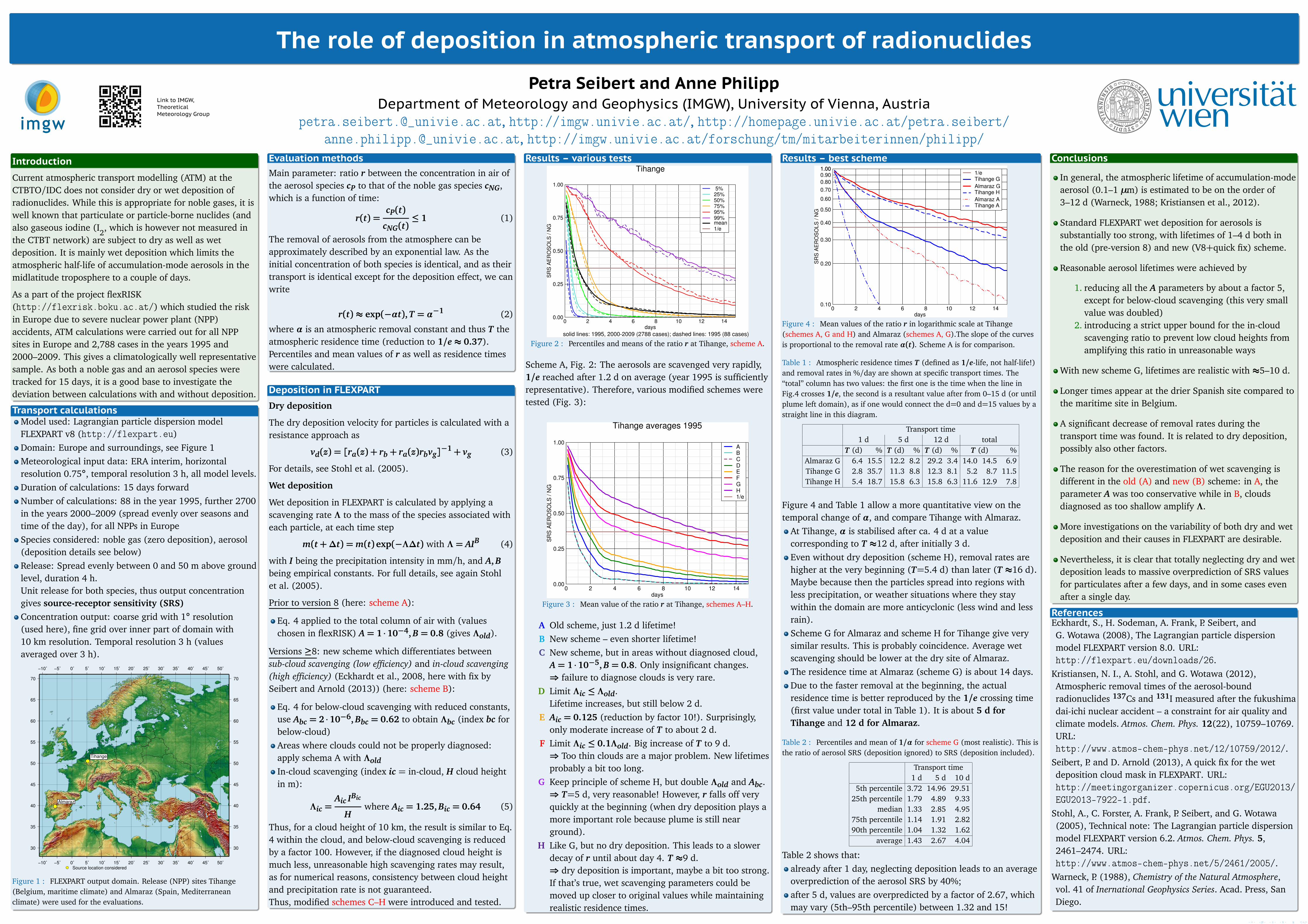
Figure 1 : FLEXPART output domain. Release (NPP) sites Tihange(Belgium, maritime climate) and Almaraz (Spain, Mediterraneanclimate) were used for the evaluations.
Evaluation methodsMain parameter: ratio r between the concentration in air ofthe aerosol species cP to that of the noble gas species cNG,which is a function of time:
r(t) =cP(t)
cNG(t)≤ 1 (1)
The removal of aerosols from the atmosphere can beapproximately described by an exponential law. As theinitial concentration of both species is identical, and as theirtransport is identical except for the deposition effect, we canwrite
r(t) ≈ exp(−αt),T = α−1 (2)
where α is an atmospheric removal constant and thus T theatmospheric residence time (reduction to 1/e ≈ 0.37).Percentiles and mean values of r as well as residence timeswere calculated.
Deposition in FLEXPART
Dry deposition
The dry deposition velocity for particles is calculated with aresistance approach as
vd(z) = [ra(z) + rb+ ra(z)rbvg]−1+ vg (3)
For details, see Stohl et al. (2005).
Wet deposition
Wet deposition in FLEXPART is calculated by applying ascavenging rate Λ to the mass of the species associated witheach particle, at each time step
m(t+∆t) =m(t)exp(−Λ∆t) with Λ = AIB (4)
with I being the precipitation intensity in mm/h, and A,Bbeing empirical constants. For full details, see again Stohlet al. (2005).
Prior to version 8 (here: scheme A):
Eq. 4 applied to the total column of air with (valueschosen in flexRISK) A = 1 ·10−4,B = 0.8 (gives Λold).
Versions ≥8: new scheme which differentiates betweensub-cloud scavenging (low efficiency) and in-cloud scavenging(high efficiency) (Eckhardt et al., 2008, here with fix bySeibert and Arnold (2013)) (here: scheme B):
Eq. 4 for below-cloud scavenging with reduced constants,use Abc = 2 ·10−6,Bbc = 0.62 to obtain Λbc (index bc forbelow-cloud)Areas where clouds could not be properly diagnosed:apply schema A with ΛoldIn-cloud scavenging (index ic = in-cloud, H cloud heightin m):
Λic =Aic IBic
Hwhere Aic = 1.25,Bic = 0.64 (5)
Thus, for a cloud height of 10 km, the result is similar to Eq.4 within the cloud, and below-cloud scavenging is reducedby a factor 100. However, if the diagnosed cloud height ismuch less, unreasonable high scavenging rates may result,as for numerical reasons, consistency between cloud heightand precipitation rate is not guaranteed.Thus, modified schemes C–H were introduced and tested.
Results – various tests
0 2 4 6 8 10 12 14days
0.00
0.25
0.50
0.75
1.00
SR
S A
ER
OS
OLS
/ N
G
solid lines: 1995, 2000-2009 (2788 cases); dashed lines: 1995 (88 cases)
5%25%50%75%95%99%mean1/e
Tihange
Figure 2 : Percentiles and means of the ratio r at Tihange, scheme A.
Scheme A, Fig. 2: The aerosols are scavenged very rapidly,1/e reached after 1.2 d on average (year 1995 is sufficientlyrepresentative). Therefore, various modified schemes weretested (Fig. 3):
0 2 4 6 8 10 12 14days
0.00
0.25
0.50
0.75
1.00
SR
S A
ER
OS
OLS
/ N
G
ABCDEFGH1/e
Tihange averages 1995
Figure 3 : Mean value of the ratio r at Tihange, schemes A–H.
A Old scheme, just 1.2 d lifetime!B New scheme – even shorter lifetime!C New scheme, but in areas without diagnosed cloud,
A = 1 ·10−5,B = 0.8. Only insignificant changes.⇒ failure to diagnose clouds is very rare.
D Limit Λic ≤ Λold.Lifetime increases, but still below 2 d.
E Aic = 0.125 (reduction by factor 10!). Surprisingly,only moderate increase of T to about 2 d.
F Limit Λic ≤ 0.1Λold. Big increase of T to 9 d.⇒ Too thin clouds are a major problem. New lifetimesprobably a bit too long.
G Keep principle of scheme H, but double Λold and Abc.⇒ T=5 d, very reasonable! However, r falls off veryquickly at the beginning (when dry deposition plays amore important role because plume is still nearground).
H Like G, but no dry deposition. This leads to a slowerdecay of r until about day 4. T ≈9 d.⇒ dry deposition is important, maybe a bit too strong.If that’s true, wet scavenging parameters could bemoved up closer to original values while maintainingrealistic residence times.
Results – best scheme
0 2 4 6 8 10 12 14days
0.10
0.20
0.30
0.40
0.50
0.60
0.70
0.80
0.901.001.00
SR
S A
ER
OS
OL
S /
NG
1/eTihange G
Almaraz GTihange H
Almaraz ATihange A
Averages 1995
Figure 4 : Mean values of the ratio r in logarithmic scale at Tihange(schemes A, G and H) and Almaraz (schemes A, G).The slope of the curvesis proportional to the removal rate α(t). Scheme A is for comparison.
Table 1 : Atmospheric residence times T (defined as 1/e-life, not half-life!)and removal rates in %/day are shown at specific transport times. The“total” column has two values: the first one is the time when the line inFig.4 crosses 1/e, the second is a resultant value after from 0–15 d (or untilplume left domain), as if one would connect the d=0 and d=15 values by astraight line in this diagram.
Transport time1 d 5 d 12 d total
T (d) % T (d) % T (d) % T (d) %Almaraz G 6.4 15.5 12.2 8.2 29.2 3.4 14.0 14.5 6.9Tihange G 2.8 35.7 11.3 8.8 12.3 8.1 5.2 8.7 11.5Tihange H 5.4 18.7 15.8 6.3 15.8 6.3 11.6 12.9 7.8
Figure 4 and Table 1 allow a more quantitative view on thetemporal change of α, and compare Tihange with Almaraz.
At Tihange, α is stabilised after ca. 4 d at a valuecorresponding to T ≈12 d, after initially 3 d.Even without dry deposition (scheme H), removal rates arehigher at the very beginning (T=5.4 d) than later (T ≈16 d).Maybe because then the particles spread into regions withless precipitation, or weather situations where they staywithin the domain are more anticyclonic (less wind and lessrain).Scheme G for Almaraz and scheme H for Tihange give verysimilar results. This is probably coincidence. Average wetscavenging should be lower at the dry site of Almaraz.The residence time at Almaraz (scheme G) is about 14 days.Due to the faster removal at the beginning, the actualresidence time is better reproduced by the 1/e crossing time(first value under total in Table 1). It is about 5 d forTihange and 12 d for Almaraz.
Table 2 : Percentiles and mean of 1/α for scheme G (most realistic). This isthe ratio of aerosol SRS (deposition ignored) to SRS (deposition included).
Transport time1 d 5 d 10 d
5th percentile 3.72 14.96 29.5125th percentile 1.79 4.89 9.33
median 1.33 2.85 4.9575th percentile 1.14 1.91 2.8290th percentile 1.04 1.32 1.62
average 1.43 2.67 4.04
Table 2 shows that:already after 1 day, neglecting deposition leads to an averageoverprediction of the aerosol SRS by 40%;after 5 d, values are overpredicted by a factor of 2.67, whichmay vary (5th–95th percentile) between 1.32 and 15!
Conclusions
In general, the atmospheric lifetime of accumulation-modeaerosol (0.1–1 µm) is estimated to be on the order of3–12 d (Warneck, 1988; Kristiansen et al., 2012).
Standard FLEXPART wet deposition for aerosols issubstantially too strong, with lifetimes of 1–4 d both inthe old (pre-version 8) and new (V8+quick fix) scheme.
Reasonable aerosol lifetimes were achieved by
1. reducing all the A parameters by about a factor 5,except for below-cloud scavenging (this very smallvalue was doubled)
2. introducing a strict upper bound for the in-cloudscavenging ratio to prevent low cloud heights fromamplifying this ratio in unreasonable ways
With new scheme G, lifetimes are realistic with ≈5–10 d.
Longer times appear at the drier Spanish site compared tothe maritime site in Belgium.
A significant decrease of removal rates during thetransport time was found. It is related to dry deposition,possibly also other factors.
The reason for the overestimation of wet scavenging isdifferent in the old (A) and new (B) scheme: in A, theparameter A was too conservative while in B, cloudsdiagnosed as too shallow amplify Λ.
More investigations on the variability of both dry and wetdeposition and their causes in FLEXPART are desirable.
Nevertheless, it is clear that totally neglecting dry and wetdeposition leads to massive overprediction of SRS valuesfor particulates after a few days, and in some cases evenafter a single day.
ReferencesEckhardt, S., H. Sodeman, A. Frank, P. Seibert, andG. Wotawa (2008), The Lagrangian particle dispersionmodel FLEXPART version 8.0. URL:http://flexpart.eu/downloads/26.
Kristiansen, N. I., A. Stohl, and G. Wotawa (2012),Atmospheric removal times of the aerosol-boundradionuclides 137Cs and 131I measured after the fukushimadai-ichi nuclear accident – a constraint for air quality andclimate models. Atmos. Chem. Phys. 12(22), 10759–10769.URL:http://www.atmos-chem-phys.net/12/10759/2012/.
Seibert, P. and D. Arnold (2013), A quick fix for the wetdeposition cloud mask in FLEXPART. URL:http://meetingorganizer.copernicus.org/EGU2013/EGU2013-7922-1.pdf.
Stohl, A., C. Forster, A. Frank, P. Seibert, and G. Wotawa(2005), Technical note: The Lagrangian particle dispersionmodel FLEXPART version 6.2. Atmos. Chem. Phys. 5,2461–2474. URL:http://www.atmos-chem-phys.net/5/2461/2005/.
Warneck, P. (1988), Chemistry of the Natural Atmosphere,vol. 41 of Inernational Geophysics Series. Acad. Press, SanDiego.