PETE 603

Lecture Session #30

Thursday, 7/29/10

30.2 Accuracy of Solutions

• Material Balance Error• Nonlinear Error• Instability Error• Truncation Error• Roundoff Error• Numerical Dispersion• Grid Orientation

30.3 Material Balance Error

tq + B

SV -

B

SV = MBE Local o

ji,o

opn

o

op1+n

ji,

1n

1 ijo

o

o

p1n

o

op

ijtq

B

SV

B

SVCum.MBE

o

• Over a single timestep

• Over entire simulation

30.4 Material Balance ErrorCauses of material balance error:

- non-conservative equation formulation

- error in solution of nonlinear equations

(Newton-Raphson)

- error in matrix solutions

- roundoff errors (numerical precision)

- data errors (negative compressibilities)

- program bugs

30.5 Nonlinear Error

Interpolating PVT functions linearly is a source of error.

Data points in PVT table

Pressure

PVT quantity

True PVT data

30.6 Nonlinear Error

• Nonlinear errors are especially a problem near the bubblepoint due to discontinuity in total compressibility.

• Chord slopes in IMPES

• Solutions:– take smaller timesteps– iterate on chord slope (IMPES)

ni

nif

np

np ppcVV 11 1

30.7 Instability Error

Sw

TimeIf a simulation run becomes unstable erroneous saturations will occur.

30.8 Instability Error

• Caused by taking timesteps which are too large in an IMPES method.

• Solution:– Take smaller timesteps– Use fully implicit method

30.9 Truncation Error

x - x

f(x) - )x+f(x= (x)f O

.... + (x)f

3!x

- (x)f 2!x

- x

f(x) - x)+f(x= (x)f

2

Truncating the Taylor series expansions is a source of error.

The size of this error depends on the grid size and the timestep.

30.10 Truncation Error1,000

800

600

400

2000 20 40 60 80

PR

ES

SU

RE

(X

= 1

00 l

l ),

psi

a

TIME, days

DELT

10 days

5 days

1.25 days

0.15 days

Refining the grid and/or reducing the timestep reduces the truncation error.

30.11 Numerical Dispersion

Numerical dispersion causes fluid fronts to arrive sooner than they should. Fronts that should be sharp become smeared.

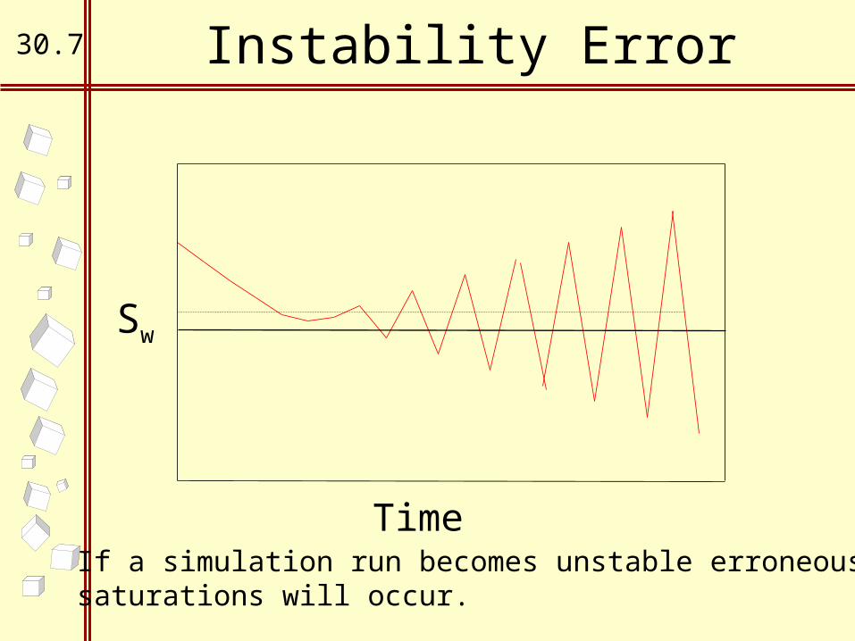
30.12 Numerical Dispersion

• Solution:– Use smaller gridblocks– Upstream relative permeabilities also help

minimize numerical dispersion.• Multipoint upstream sometimes used in tracer

studies

– Use pseudorelative permeabilities (pseudofunctions)

– Choose timestep wisely in IMPES (maximum stable timestep)

30.13 Numerical Dispersion

• Do we want to remove numerical dispersion altogether?

• Buckley-Leverett flow does not apply for many field cases.– Capillary pressure spreads out fluid front,

especially in low permeability reservoirs.– Permeability heterogeneity smears fluid

front (fingering).

• Some numerical dispersion may be acceptable.

30.14 Grid Orientation

The orientation of the grid with respect to the well locations can influence the simulation results.

Fluid moves preferentially along the grid lines. If the red dot represented a water injector, the water would break through fastest in the diagonal grid (right) - even if the grid dimensions were the same.

30.15 Grid Orientation• To overcome the grid orientation effect a different form of the finite-difference method can be used.

• The usual method is called the “five-point” approach.

• The “nine-point” approach to the flow equations removes the grid orientation effect, however more computational work is required.

• The “Control Volume Finite Element” approach often uses triangular gridblocks (full permeability tensor required).

30.16 Grid Orientation

30.17 Grid Orientation

30.18 Data Modification - 5 spot

Injector

ProducerProducer

ProducerProducer

30.19 Data Modification - 5 spot

Simulator: Quarter 5-spot

30.20 Data Modification - 5 spot

ky

kx

2

2

Data Modification: Quarter 5-spot

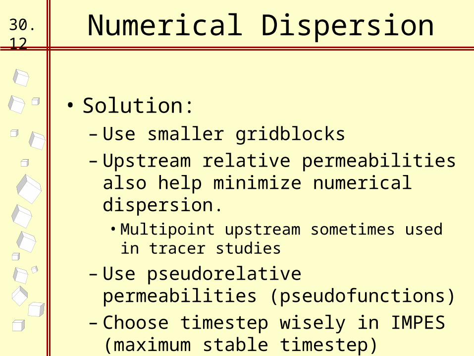
30.21 Data Modification - 5 spot

Final Result: Quarter 5-spot