Frank TsungViktor K. Decyk

Weiming AnXinlu Xu

Diana Amorim (IST)

Warren Mori (PI)

Petascale Particle-in-Cell Simulation of Laser Plasma Interactions in High Energy Density Plasmas on Blue

Waters

Summary and Outline OUTLINE/SUMMARY

· Overview of the project· Particle-in-cell method · OSIRIS

· Application of OSIRIS to plasma based accelerators:· QuickPIC simulations of positron experiments @ SLAC· LWFA’s in the self-modulated regime @ Livermore National

Laboratory

· Higher (2 & 3) dimension simulations of LPI’s relevant to laser fusion· Suppression of SRS with an external magnetic field· Controlling LPI’s by frequency bandwidth.· Estimates of large scale LPI simulations (& justify the need for

new numerical techniques and new algorithms and exascale supercomputers)

· Code Developments to reduce simulation time and to move toward exa-scale.· Quasi-3D OSIRIS for LWFA and single-speckle LPI

simulations on blue waters· code development efforts for GPU’s and Intel PHI’s.· PICKSC Center @ UCLA , which provides a resource for

anyone interested in learning about PIC

Profile of OSIRIS + Introduction to PIC

• The particle-in-cell method treats plasma as a collection of computer particles. The interactions does not scale as N2 due to the fact the particle quantities are deposited on a grids and the interactions are calculated on the grids only. Because (# of particles) >> (# of grids), the timing is dominated by the particle calculations and scales as N (orbit calculation + current & charge deposition).

• The code spends over 90 % of execution time in only 4 routines

• These routines correspond to less than 2 % of the code, optimization and porting is fairly straightforward, although not always trivial.

PIC algorithm

Δt

Integration of equations of motion, moving particles

Interpolation

Integration of Field Equations on the grid

Fi → ui → xi

Jj →( E , B )j

( E , B )j → Fi

Current

Deposition

(x,u)j → Jj

Field interpolation

42.9% time, 290 lines

Current deposition

35.3% time, 609 lines

Particle du/dt

9.3% time, 216 lines

Particle dx/dt

5.3% time, 139 lines

code features

· Scalability to ~ 1.6 M cores (on sequoia) and achieved sustained speed of > 2.2PetaFLOPS on Blue Waters

· SIMD hardware optimized· Parallel I/O· Dynamic Load Balancing· QED module· Particle merging· OpenMP/MPI parallelism· CUDA/Xeon Phi branches

osiris framework· Massivelly Parallel, Fully Relativistic

Particle-in-Cell (PIC) Code · Visualization and Data Analysis

Infrastructure· Developed by the osiris.consortium

⇒ UCLA + IST

Ricardo Fonseca: ricardo.fonseca@tecnico.ulisboa.ptFrank Tsung: tsung@physics.ucla.eduhttp://epp.tecnico.ulisboa.pt/ http://plasmasim.physics.ucla.edu/

O i ir ss3.0

Laser Wake Field Accelerator(LWFA, SMLWFA) A single short-pulse of photons

Plasma Wake Field Accelerator(PWFA) A high energy electron bunch

Livingston Curve for Accelerators --- Why plasmas?

Drive beamTrailing beam

The Livingston curve traces the history of electron accelerators from Lawrence’s cyclotron to present day technology.

When energies from plasma based accelerators are plotted in the same curve, it shows the exciting trend that within a few years it is will surpass conventional accelerators in terms of energy.

FACET is a new facility to provide high-energy, high peak current e- & e+ beams for PWFA experiments at SLAC.

FACET— Plasma based accelerator experiments @ LCLS (linac coherent light source)

Facility for Advanced aCcelerator Experimental Tests

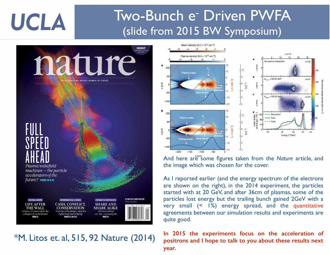
Two-Bunch e- Driven PWFA(slide from 2015 BW Symposium)

*M. Litos et. al, 515, 92 Nature (2014)

And here are some figures taken from the Nature article, and the image which was chosen for the cover.

As I reported earlier (and the energy spectrum of the electrons are shown on the right), in the 2014 experiment, the particles started with at 20 GeV, and after 36cm of plasmas, some of the particles lost energy but the trailing bunch gained 2GeV with a very small (< 1%) energy spread, and the quantitative agreements between our simulation results and experiments are quite good.

In 2015 the experiments focus on the acceleration of positrons and I hope to talk to you about these results next year.

So what about positrons?

Positrons beams produce wakes which are very different than those produced by electron beams (because the plasma is not made of anti-matter). On top is a possible plasma based collider using plasmas. On the left is nonlinear plasma wave generated by electrons. On the right you see nonlinear plasma wave generated by positrons. And as you can see the wake structures are very different.

For an electron beam, the beam pushes away all of the nearby electrons, forming a spherical wake which is called a “bubble”. On the other hand, positrons will pull in all of the nearby electrons, forming a very different looking wake. The theory for plasma wakes due to a positron beam is not well developed and Blue Water simulations play a very important role in giving us insights to these experiments using positron beams.

Acceleration of positrons @ SLAC

Experiments produced beams with very low energy spread (as low as 1.8% to 4% and 6% in the plots shown above). In 1.3 meters, the positrons gained 3-10GeV’s, varying from shot to shot (compared to .1GeV/meter inside a conventional accelerator).

QuickPIC simulations revealed the physics of the low energy spread seen in experiments. On the right the 2D electron density and the axial accelerating field are plotted. On the left is a snapshot from our QuickPIC simulation, showing electron phase space (lower left) and densities + accelerating field on axis + densities (upper left) QuickPIC simulation showed that, the trailing bunch flattens the wake, producing a uniform field that accelerates the trailing electrons uniformly.*S. Corde et. al, 524, 442 Nature(2015).

F. S. Tsung, Blue Waters 2016

TITAN current experiment @ LLNL

Massively parallel PIC code OSIRIS used for thorough and high resolution investigation of 3D effects in the support of the laser wakefield accelerator exp. @ LLNL

➡The laser produces ~200 MeV electrons, but it is useful in producing directional (forward-going), hard X-rays

➡ using the 150J and 1ps long Titan laser infrastructure available at LLNL

➡ 3D effects (shown below)

➡This work is ongoing and we will share more results with you at next year’s BW symposium

Rad

iatio

n em

itted

by

e- s

Ener

gy s

pect

rum

of r

adia

tion

To benchmark the experiment 3D simulations taking (30 billion grids, 1 trillion particles) up to

460 800 core-hours were required

3D effects have impact on final radiation

That shows X-rays featuresPl

asm

a w

ake

of e

- s plasma e-s

laser beamenergetic electron orbits

Laser Plasma Interactions

Laser Plasma Interactions in IFE

NIFNational Ignition Facility

IFE (inertial fusion energy) uses lasers to compress fusion pellets to fusion conditions. The goal of these experiments is to extract more fusion energy from the fuel than the input energy of the laser. In this case, the excitation of plasma waves via LPI (laser plasma interactions) is detrimental to the experiment in 2 ways.

Laser light can be scattered backward toward the source and cannot reach the target

LPI produces hot electrons which heats the target, making it harder to compress.

The LPI problem is very challenging because it spans many orders of magnitude in lengthscale & lengthscale

The spatial scale spans from < 1 micron (which is the laser wavelength) to mille-meters (which is the length of the plasma).

The temporal scale spans from a femto-second(which is the laser period) to nano-seconds (which is the duration of the fusion pulse). A typical PIC simulation spans ~10ps.

Lengthscales

speckle width1μm

Inner Beam Path (>1mm)

laser wavelength (350nm)

10μm

speckle length

100μm 1mm

Timescales

LPI growth time

1fs 1ps 1ns

NIF pulse (20ns)

Final laserspike (1ns)

non-linear interactions(wave/wave, wave particle,and multiple speckles) ~10ps

Laser period (1fs)

Performing a typical 1D OSIRIS Simulation Using NIF parameters

• Currently, experimentalists @ NIF can re-construct plasma conditions (such as density and temperature) using a hydro code. Using this “plasma map”, we can perform a series of 1D OSIRIS simulations, each taking ~100 CPU hours.

• 1D OSIRIS Simulations can predict:

• Spectrum of backscattered lights (which can be compared against experiments)

• spectrum of energetic electrons (shown below) • energy partition, i.e., how the incident laser energy is converted to

• transmitted light • backscattered light • energetic electrons

Ilaser = 2 – 8 x 1014 W/cm2

λlaser = 351nm, Te = 2.75 keV, Ti = 1 keV, Z=1,tmax up to 20 psLength = 1.5 mmDensity profiles from NIFhydro simulations

14 million particles~100 CPU hours per run~1 hr on modest size

supercomputer

I0=4e14,Greenprofile

Due to backscatter

Due to LDI of backscatter

I0=8e14,Redprofile

DuetoLDIofresca;er

Duetoresca;erofini=alSRS

Laser direction

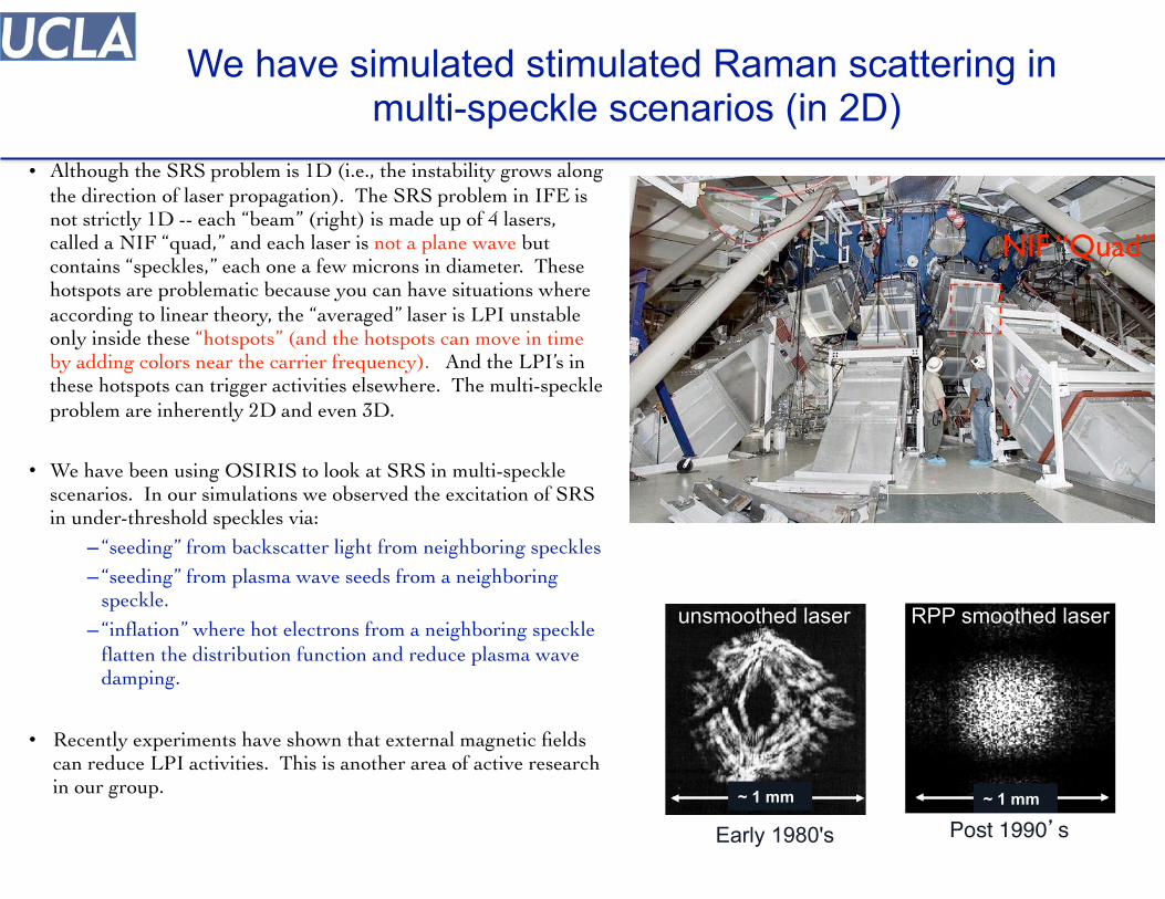
We have simulated stimulated Raman scattering in multi-speckle scenarios (in 2D)

NIF “Quad”

• Although the SRS problem is 1D (i.e., the instability grows along the direction of laser propagation). The SRS problem in IFE is not strictly 1D -- each “beam” (right) is made up of 4 lasers, called a NIF “quad,” and each laser is not a plane wave but contains “speckles,” each one a few microns in diameter. These hotspots are problematic because you can have situations where according to linear theory, the “averaged” laser is LPI unstable only inside these “hotspots” (and the hotspots can move in time by adding colors near the carrier frequency). And the LPI’s in these hotspots can trigger activities elsewhere. The multi-speckle problem are inherently 2D and even 3D.

• We have been using OSIRIS to look at SRS in multi-speckle scenarios. In our simulations we observed the excitation of SRS in under-threshold speckles via:

– “seeding” from backscatter light from neighboring speckles– “seeding” from plasma wave seeds from a neighboring

speckle.– “inflation” where hot electrons from a neighboring speckle

flatten the distribution function and reduce plasma wave damping.

• Recently experiments have shown that external magnetic fields can reduce LPI activities. This is another area of active research in our group.

| Los Alamos National Laboratory |

July 2013 | UNCLASSIFIED | 19 Operated by Los Alamos National Security, LLC for the U.S. Department of Energy's NNSA

Beam smoothing in the 80ʼs – 90ʼs introduced additional control for LPI by modulating the laser beam structure

Early 1980's

unsmoothed laser

~ 1 mm

RPP smoothed laser

~ 1 mm

Post 1990�s"

SSD effects on SRS in exploding foils

• Pioneering expts RPP – Kato et al., PRL (1984)"• Pioneering expts & theory ISI – Obenschain et al., PRL (1989)"• Detailed expts & theory on Nova show role of hot spots" and self-focusing in LPI growth (SSD)"

"- Rose & DuBois PRL (1994)""- Berger et al. PRL (1995)""- Moody et al. PoP (1995)""- Montgomery et al. PoP (1996)""- MacGowan et al. PoP (1996)"

Montgomery et al. PoP (1996)"

F. S. Tsung, Blue Waters 2016

Control of TPD/HFHI instability by adding > THz bandwidth

Laser Profile Transmitted Light

Continuous <20

300fs, 25%DC 43.8

300fs, 50%DC 50.7

One technique to “smooth” the laser profile is to add frequency bandwidth to the laser so the speckle pattern changes over time. This has the effects of smoothing the laser profile in a time-averaged sense and reduce hydrodynamical instabilities. We have begun to look at the effects of temporal bandwidths on laser plasma instabilities.

In simulations where the inverse temporal bandwidth is comparable to the growth time of the instability, simulations showed that:

1. The plasma wave activity and the interaction region is much smaller with the addition of the temporal bandwidth, and

2. most of the light is transmitted during the linear phase of the instability, which leads to more of the lights going past the quarter critical layer and reaching the fusion target. In simulations without bandwidth, only ~20% of the light makes it to the target, and about 50% of the light makes it to the target when a 3THz bandwidth is present.

Tim

e

z (laser prop. direction)

nc/4

14

PIC simulations of 3D LPI’s is still a challenge, and requires exa-scale supercomputers, this will require code developments in both new numerical methods and new codes for new hardwares

2D multi-speckle along NIF beam path 3D, 1 speckles 3D, multi-speckle along

NIF beam path

Speckle scale 50 x 8 1 x 1 x 1 10 x 10 x 5

Size (microns) 150 x 1500 9 x 9 x 120 28 x 28 x 900

Grids 9,000 x 134,000 500 x 500 x 11,000 1,700 x 1,700 x 80,000

Particles 300 billion 300 billion 22 trillion

Steps 470,000 (15 ps) 540,000 (5 ps) 540,000 (15 ps)

Memory Usage* 7 TB 6 TB 1.6 PB

CPU-Hours 8 million 13 million 1 billion (2 months on the full BW)

2D Cylindrical OSIRIS with Azimuthal Modal Decomposition (Ref: Davidson et al, JCP 281, 1063

(2015))• LPI’s with a single laser speckle (and the 3D LWFA problem) , the incident laser and the

excited plasma waves are mostly cylindrically symmetric. We would like to take advantage of this property but lasers are not polarized in or (but rather in or ), so a simple (r,z) code is insufficient.

• Following Lifschitz et. al*, we developed the ability to model plasmas in 3D using cylindrical coordinates (r,z,φ) by introducing a Fourier decomposition in the φ (azimuthal angle) dimension

• This representation, and the identity:

means that we can represent a linearly polarized laser with one additional mode. This decomposition enables us to study 3D physics for a variety of problems described here at a great saving (i.e., at a cost of running several 2D simulations).

We have extended this work of Lifschitz et al to enforce charge conservation in the current deposition, thereby eliminating the need to solve Poisson’s equation.

The 3D field values (E, B, J) are decomposed into azimuthal modes (Em, Bm, Jm), each one

is a function of (r,z)

Ex

= Er

cos(�) + E�

sin(�) Ey = �Er sin(�) + E� cos(�)

rx

y

*Lifschitz et al, JCP 228, 1803 (2008).

�

Comparison Between 3D & 2D Hybrid(electron density)

0 800ξ [c/ω ]0

0

400

x [c

/ω ] 0

n/n c

0

0.01

3D 2D hybrid

0

400

r [c/

ω ] 0

1mm

0 800ξ [c/ω ]0

0 800ξ [c/ω ]0

0

400

x [c

/ω ] 0

9mm

n/n c

0

0.01

0

400

r [c/

ω ] 0

0 800ξ [c/ω ]0

We have applied the hybrid algorithm to some of the problems described here. We have benchmarked this code against some of our published 3D results. In this case, a plasma based accelerator with a laser driver.

As shown on the right, the 2D “hybrid” code agrees very well with previous 3D simulations, recovering the wake structure and also self-trapping physics in the equivalent 3D simulations. at a saving of 1-2 orders of magnitude. (25,000 “2015” CPU hours in 3D and 1,250 hours using 2D hybrid)

In addition to new numerical methods, we are also adapting our PIC codes to new hardwares, such as GPU’s and multi-core CPU’s

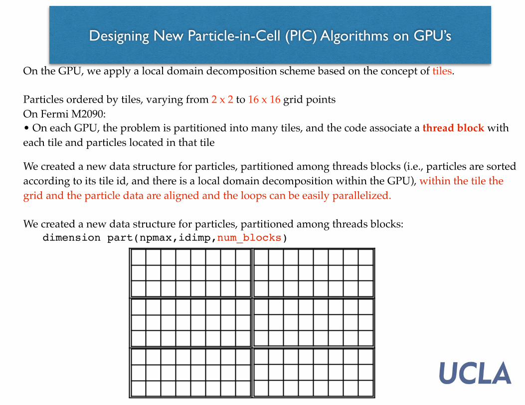
On the GPU, we apply a local domain decomposition scheme based on the concept of tiles.

Particles ordered by tiles, varying from 2 x 2 to 16 x 16 grid pointsOn Fermi M2090:• On each GPU, the problem is partitioned into many tiles, and the code associate a thread block with each tile and particles located in that tile We created a new data structure for particles, partitioned among threads blocks (i.e., particles are sorted according to its tile id, and there is a local domain decomposition within the GPU), within the tile the grid and the particle data are aligned and the loops can be easily parallelized.

We created a new data structure for particles, partitioned among threads blocks:

dimension part(npmax,idimp,num_blocks)

Designing New Particle-in-Cell (PIC) Algorithms on GPU’s

Porting PIC codes to GPU’s (continued)

Designing New Particle-in-Cell (PIC) Algorithms:

Maintaining Particle Order

Three steps:1. Particle Push creates a list of particles which are leaving a tile 2. Using list, each thread places outgoing particles into an ordered buffer it controls3. Using lists, each tile copies incoming particles from buffers into particle array

A “particle manager” is needed to maintain the data alignment. This is done every timestep.• Less than a full sort, low overhead if particles already in correct tile• Essentially message-passing, except buffer contains multiple destinations

In the end, the particle array belonging to a tile has no gaps• Particles are moved to any existing holes created by departing particles• If holes still remain, they are filled with particles from the end of the array

GPU Particle Reordering

GPU Buffer

GPU Tiles

GPU Tiles

GPU Tiles

Particles bufferedin Direction Order

21

53

6

4

7 8

1 234 5678

5

2

8

4

1

7

3

6

Evaluating New Particle-in-Cell (PIC) Algorithms on GPU: Electromagnetic Case2-1/2D EM Benchmark with 2048x2048 grid, 150,994,944 particles, 36 particles/celloptimal block size = 128, optimal tile size = 16x16

GPU algorithm also implemented in OpenMPHot Plasma results with dt = 0.04, c/vth = 10, relativistic CPU:Intel i7 GPU:Fermi M2090 OpenMP(12 CPUs)Push 66.5 ns. 0.426 ns. 5.645 ns.Deposit 36.7 ns. 0.918 ns. 3.362 ns.Reorder 0.4 ns. 0.698 ns. 0.056 ns.Total Particle 103.6 ns. 2.042 ns. 9.062 ns (11.4x speedup).

The time reported is per particle/time step.The total particle speedup on the Fermi M2090 was 51x compared to 1 Intel i7 core.

Field solver takes an additional 10% on GPU, 11% on CPU.

OK, so how about multiple CPU/GPU’s?

Evaluating New Particle-in-Cell (PIC) Algorithms on GPU: Electrostatic Case2D ES Benchmark with 2048x2048 grid, 150,994,944 particles, 36 particles/celloptimal block size = 128, optimal tile size = 16x16. Single precision. Fermi M2090 GPU

Hot Plasma results with dt = 0.1 CPU:Intel i7 1 GPU 24 GPUs 108 GPUsPush 22.1 ns. 0.327 ns. 13.4 ps. 3.46 ps.Deposit 8.5 ns. 0.233 ns. 11.0 ps. 2.60 ps.Reorder 0.4 ns. 0.442 ns. 19.7 ps. 5.21 ps.Total Particle 31.0 ns. 1.004 ns. 49.9 ps. 13.10 ps.

The time reported is per particle/time step.The total particle speedup on the 108 Fermi M2090s compared to 1 GPU was 77x (>70% efficient),

We feel that we can improve on the current efficiency. Currently, field solver (which uses FFT) takes an additional 5% on 1 GPU, 45% on 2 GPUs, and 73% on 108 GPUs. And we believe the efficiency should be higher for PIC codes with a finite-difference solver.

We are also working on a Intel Phi version!

here are available at the UCLA PICKSC web-site

http://picksc.idre.ucla.edu/

MPI Send Buffer

GPU-MPI Particle Reordering

GPU Buffer

GPU Tiles

MPI Recv Buffer

GPU 1

GPU 2

GPU Tiles

UCLA Particle-in-Cell and Kinetic Simulation Software Center (PICKSC), NSF funded center whose Goal is to provide and document parallel Particle-in-Cell (PIC) and other kinetic codes.

http://picksc.idre.ucla.edu/github: UCLA Plasma Simulation Group (currently closed)

Planned activities• Provide parallel skeleton codes for various PIC codes on traditional and new hardware systems.• Provide MPI-based production PIC codes that will run on desktop computers, mid-size clusters, and the largest parallel computers in the world.• Provide key components for constructing new parallel production PIC codes for electrostatic, electromagnetic, and other codes.• Provide interactive codes for teaching of important and difficult plasma physics concepts• Facilitate benchmarking of kinetic codes by the physics community, not only for performance, but also to compare the physics approximations used• Documentation of best and worst practices for code writing, which are often unpublished and get repeatedly rediscovered. • Provide some services for customizing software for specific purposes (based on our existing codes) Key components and codes will be made available through standard open source licenses and as an open-source community resource, contributions from others are welcome.

Summary and Outline OUTLINE/SUMMARY

· Overview of the project· Particle-in-cell method · OSIRIS

· Application of OSIRIS to plasma based accelerators:· QuickPIC simulations of positron experiments @ SLAC· LWFA’s in the self-modulated regime

· Higher (2 & 3) dimension simulations of LPI’s relevant to laser fusion· Suppression of SRS with an external magnetic field· Controlling LPI’s by frequency bandwidth.· Estimates of large scale LPI simulations (& justify the need for

new numerical techniques and new algorithms and exascale supercomputers)

· Code Developments to reduce simulation time and to move toward exa-scale.· Quasi-3D OSIRIS for LWFA and single-speckle LPI

simulations on blue waters· code development efforts for GPU’s and Intel PHI’s.· PICKSC Center @ UCLA , which provides a resource for

anyone interested in learning about PIC

Special Thanks to the Blue Waters team for its continuing technical support and its seemingly unlimited computer time!

F. S. Tsung, Blue Waters 2016

Control of TPD/HFHI instability by adding > THz bandwidth

Laser Profile Transmitted Light

Continuous <20

300fs, 25%DC 43.8

300fs, 50%DC 50.7

One technique to “smooth” the laser profile is to add frequency bandwidth to the laser so the speckle pattern changes over time. This has the effects of smoothing the laser profile in a time-averaged sense and reduce hydrodynamical instabilities. We have begun to look at the effects of temporal bandwidths on laser plasma instabilities.

In simulations where the inverse temporal bandwidth is comparable to the growth time of the instability, simulations showed that:

1. The plasma wave activity and the interaction region is much smaller with the addition of the temporal bandwidth, and

2. most of the light is transmitted during the linear phase of the instability, which leads to more of the lights going past the quarter critical layer and reaching the fusion target. In simulations without bandwidth, only ~20% of the light makes it to the target, and about 50% of the light makes it to the target when a 3THz bandwidth is present.

Tim

e

z (laser prop. direction)

nc/4

25