
Perturbing the boundary conditions of the generator of a cosine family
17
Semigroup Forum (2012) 85:58–74 DOI 10.1007/s00233-011-9361-3 RESEARCH ARTICLE Perturbing the boundary conditions of the generator of a cosine family Edgardo Alvarez-Pardo Received: 19 July 2011 / Accepted: 22 November 2011 / Published online: 7 December 2011 © Springer Science+Business Media, LLC 2011 Abstract Let A be a densely defined, closed linear operator (which we shall call maximal operator) with domain D(A) on a Banach space X and consider closed lin- ear operators L : D(A) → ∂X and : D(A) → ∂X (where ∂X is another Banach space called boundary space). Putting conditions on L and , we show that the sec- ond order abstract Cauchy problem for the operator A with A u = Au and domain D(A ) := {u ∈ D(A) : Lu = u} is well-posed and thus it generates a cosine opera- tor function on the Banach space X. Keywords Cosine functions · Abstract Cauchy problems · General boundary conditions · Analytic C 0 -semigroups 1 Introduction Given a closed and densely defined linear operator (A, D(A)) (which we shall call maximal operator) defined on a Banach space X and the closed linear operators L : D(A) → ∂X and : D(A) → ∂X where ∂X is another Banach space called boundary space, we consider the second order abstract Cauchy problem for the op- erator A with domain given by D(A ) := {u ∈ D(A) : Lu = u} and defined by A u := Au. That is, for u 0 and u 1 in X we consider the problem u (t) =: A u(t), t ∈ R, u(0) = u 0 , u (0) = u 1 (1.1) Communicated by Jerome A. Goldstein. E. Alvarez-Pardo ( ) Facultad de Ciencias Básicas, Universidad Tecnológica de Bolivar, Cartagena, Colombia e-mail: [email protected] E. Alvarez-Pardo e-mail: [email protected]
Transcript of Perturbing the boundary conditions of the generator of a cosine family
Semigroup Forum (2012) 85:58–74DOI 10.1007/s00233-011-9361-3
R E S E A R C H A RT I C L E
Perturbing the boundary conditions of the generatorof a cosine family
Edgardo Alvarez-Pardo
Received: 19 July 2011 / Accepted: 22 November 2011 / Published online: 7 December 2011© Springer Science+Business Media, LLC 2011
Abstract Let A be a densely defined, closed linear operator (which we shall callmaximal operator) with domain D(A) on a Banach space X and consider closed lin-ear operators L : D(A) → ∂X and � : D(A) → ∂X (where ∂X is another Banachspace called boundary space). Putting conditions on L and �, we show that the sec-ond order abstract Cauchy problem for the operator A� with A�u = Au and domainD(A�) := {u ∈ D(A) : Lu = �u} is well-posed and thus it generates a cosine opera-tor function on the Banach space X.
Keywords Cosine functions · Abstract Cauchy problems · General boundaryconditions · Analytic C0-semigroups
1 Introduction
Given a closed and densely defined linear operator (A,D(A)) (which we shall callmaximal operator) defined on a Banach space X and the closed linear operatorsL : D(A) → ∂X and � : D(A) → ∂X where ∂X is another Banach space calledboundary space, we consider the second order abstract Cauchy problem for the op-erator A� with domain given by D(A�) := {u ∈ D(A) : Lu = �u} and defined byA�u := Au. That is, for u0 and u1 in X we consider the problem{
u′′(t) =: A�u(t), t ∈ R,
u(0) = u0, u′(0) = u1(1.1)
Communicated by Jerome A. Goldstein.
E. Alvarez-Pardo (�)Facultad de Ciencias Básicas, Universidad Tecnológica de Bolivar, Cartagena, Colombiae-mail: [email protected]
E. Alvarez-Pardoe-mail: [email protected]
Perturbing the boundary conditions of the generator of a cosine family 59
If we assume that the problem is well-posed for � ≡ 0, i.e., the problem{u′′(t) =: A0u(t), t ∈ R,
u(0) = u0, u′(0) = u1(1.2)
is well-posed, then the following problem arises. For which conditions on L and �
is the problem well-posed again?For the first order abstract Cauchy problem, Greiner and Kuhn made a complete
study (generation of C0-semigroup and holomorphy) and they obtained useful results,e.g., [5, 6]. In the first paper, Greiner used the Dirichlet operator and similarity tech-niques to prove generation results. The other paper treats about the analytic case. Thistime, the relationship between interpolation theory and semigroups was fundamentalin order to obtain the outcomes.
Later, Nickel proved the same generation results by using the theory of operatormatrices. Also, this author has been used the method of dynamical systems as analternative tool to prove some of this results.
For the second order problem, related cases of this problem have been investigatedby Keyantuo and Warma in [8, 9], Chill (and the preceding authors) in [3], Bátkai andEngel in [2], Xiao and Liang in [14] among others.
Greiner and Kuhn used the semigroup theory to prove the wellposedness of thefirst abstract Cauchy problem corresponding to the operator A�. The aim of thispaper is to obtain the analogous results corresponding to the second order abstractCauchy problem by using cosine operator functions.
This paper is organized as follows. In Sect. 2, we give some definitions and fun-damental results related with semigroups, cosine operator functions and perturbationtheory. In Sect. 3, we state and prove the main theorems concerning to (1.2) takingdifferent phase spaces V0 corresponding to the problem that involves A0. In Sect. 4,we present the approach of dynamical systems and multiplicative perturbation forobtain generation theorems. In Sect. 5, we give some examples and remarks.
2 Preliminaries
Definition 2.1 Let X be a Banach space. A strongly continuous function C : R →L(X) is called a cosine operator function if it satisfies the D’Alembert functionalequation:
(1) C(t + s) + C(t − s) = 2C(t)C(s) for all s, t ∈ R,(2) C(0) = IX .
As for the case of C0-semigroups, it is possible to associate to any cosine operatorfunction a unique generator in the following way.
Definition 2.2 Consider a cosine operator function (C(t))t∈R on a Banach space X.Then the generator of C(t) is given by
Ax := limt→0
2
t2
(C(t)x − x
), D(A) :=
{x ∈ X : lim
t→0
2
t2
(C(t)x − x
)exists
}.
60 E. Alvarez-Pardo
To every cosine operator function (C(t))t∈R is associated another strongly con-tinuous family operators (S(t))t∈R which is called sine operator function, and it isdefined as follows.
Definition 2.3 Let (C(t))t∈R be a cosine operator function on a Banach space X.Then we define the associated sine operator function (S(t))t∈R by
S(t)x :=∫ t
0C(s)xds, t ∈ R, x ∈ X.
In the fundamental paper [10], J. Kisynski studied the relationship between cosinefunctions and strongly continuous groups of operators. He obtained the followingtheorem.
Theorem 2.4 (Kisynski) Let X be a Banach space, and let A be a closed linearoperator on X. Then the following assertions are equivalent:
(i) The operator A is the generator of a cosine family (C(t))t∈R.(ii) There exists a Banach space V such that D(A) ↪→ V ↪→ X (where D(A) is
equipped with the graph norm) and such that the operator
A =(
0 I
A 0
)
with domain D(A) × V generates a strongly continuous semigroup in V × X. TheBanach space V is called the Kisynski space and is uniquely determined by (ii). Thespace V × X is called the phase space associated with (C(t))t∈R.
Sometimes, we put (C(t,A))t∈R to specify that the generator of the family(C(t))t∈R is the operator A.
The following result appears in [11, Lemma 2.4].
Lemma 2.5 Let V1,V2,X1,X2 be Banach spaces with V1 ↪→ X1 and V2 ↪→ X2 andlet U be an isomorphism from V1 onto V2 and from X1 onto X2. Then an operatorA generates a cosine operator function with associated phase space V1 × X1 if andonly if UAU−1 generates a cosine operator function with phase space V2 × X2. Inthis case, there holds
UC(t,A)U−1 = C(t,UAU−1), t ∈ R.
In analogy with semigroups, we present the next perturbation results. The first oneappears in [1, Corollary 3.14.13].
Lemma 2.6 Let A be a generator of a cosine operator function with associated phasespace V ×X. Then A+B generates a cosine operator function with associated phasespace V × Xas well, provided B is an operator that is either bounded from [D(A)]to V, or bounded from V to X.

Perturbing the boundary conditions of the generator of a cosine family 61
Other result about perturbation theory for cosine functions is due to A. Rhandi.
Lemma 2.7 Let A be a generator of a cosine operator function (C(t,A))t∈R withassociated sine function (S(t,A))t∈R. If B is such that D(A) ⊂ D(B) and moreovert0 > 0 can be chosen such that
∫ t0
0‖BS(s,A)f ‖ds ≤ q‖f ‖, for all f ∈ D(A),
then also A+B generates a cosine operator function, and the associated phase spacecoincides with the phase space of A.
3 Main results
Throughout this section we consider the following.
3.1 Framework
(1) X,Y, ∂X are Banach spaces;(2) A : D(A) ⊂ X → X is a closed, densely defined linear operator (the “maximal
operator”);(3) L : [D(A)] → ∂X is linear and bounded, (here [D(A)] is the Banach space D(A)
with the graph norm ‖x‖D(A) := ‖x‖X + ‖Ax‖X); L is a surjective operator;(4) the restriction A0 := A |ker(L) generates a cosine operator function on X0 with
phase space V0 × X0 where X0 := D(A0)‖·‖X ;
(5) Y ↪→ X with Y‖·‖X = X. V0 ↪→ Y with dense embedding;
(6) D(A�) ↪→ Y with dense embedding.
3.2 The Dirichlet operator
The assumptions in the framework imply the following decomposition.
Lemma 3.1 Suppose that λ2 ∈ ρ(A0). Then D(A) = D(A0) ⊕ ker(λ2 − A). More-over, L |ker(λ2−A) is an isomorphism from ker(λ2 − A) onto ∂X.
Proof Every x ∈ D(A0) ∩ ker(λ2 − A), x �= 0 (if any) is an eigenvector of A0 corre-sponding to the eigenvalue λ2. Thus λ2 ∈ ρ(A0) implies D(A0)∩ ker(λ2 −A) = {0}.Moreover, λ2 ∈ ρ(A0) means that for every x ∈ D(A) there exists x1 ∈ D(A0) suchthat (λ2 − A)x = (λ2 − A0)x1; indeed, since the operator (λ2 − A0) is bijective,for each element (λ2 − A)x ∈ X there exists an element x1 ∈ D(A0) such that(λ2 − A)x = (λ2 − A0)x1. Thus we have x = x1 + (x − x1) where x1 ∈ D(A0) and(x − x1) ∈ ker(λ2 − A). The assertion concerning L |ker(λ2−A) follows from the factthat L is surjective and D(A0) = ker(L) by definition. �
62 E. Alvarez-Pardo
We recall the definition of the Dirichlet map. For λ2 ∈ ρ(A0), the restrictionL |ker(λ2−A) has an inverse Dλ2 : ∂X → ker(λ2 − A). That is
Dλ2 := (L |ker(λ2−A))−1,
(λ2 − A
)Dλ2 = 0, LDλ2 = I∂X. (3.1)
Note that Dλ2L is the projection of D(A) onto ker(λ2 − A) along D(A0). As a con-sequence of (3.1) we have the following result.
Lemma 3.2 Let x ∈ ∂X and λ2 ∈ ρ(A0). Then the problem{Au = λ2u
Lu = x(3.2)
admits a unique solution u := Dλ2x.
The next result shows in particular that the mapping λ �→ Dλ2 is analytic.
Lemma 3.3 Let λ2,μ2 ∈ ρ(A0). Then
Dλ2 − Dμ2 = −(λ2 − μ2)R(
λ2,A0)Dμ2 (3.3)
and
R(μ2,A0
)Dλ2 = R
(λ2,A0
)Dμ2 .
Proof Since (μ2 − A)Dμ2 = (λ2 − A)Dλ2 = 0, we have that
(λ2 − μ2)Dμ2 = λ2Dμ2 − λ2Dλ2 + ADλ2 − ADμ2
= (λ2 − A
)(Dμ2 − Dλ2)
= (λ2 − A0
)(Dμ2 − Dλ2),
where we have used that (Dμ2 − Dλ2)(∂X) ⊂ D(A0). Thus,
(λ2 − μ2)R(
λ2,A0)Dμ2 = Dμ2 − Dλ2;
and we have shown (3.3). Multiplying both sides by R(μ2,A0) and applying theresolvent identity we get the second equation in the lemma. �
The next lemma gives the relation between D(A�) and D(A0). This result will bevery important to obtain our main theorems. The proof is a simple modification of [5,Lemma 1.4].
Lemma 3.4 Suppose that λ2 ∈ ρ(A0) and f ∈ X. Then f ∈ D(A�) if and only if(I − Dλ2�)f ∈ D(A0) and we have(
λ2 − A�
)f = (
λ2 − A0)(I − Dλ2�)f.
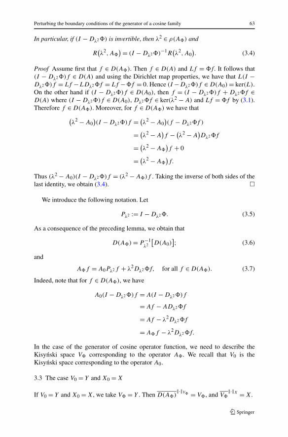
Perturbing the boundary conditions of the generator of a cosine family 63
In particular, if (I − Dλ2�) is invertible, then λ2 ∈ ρ(A�) and
R(λ2,A�
) = (I − Dλ2�)−1R(λ2,A0
). (3.4)
Proof Assume first that f ∈ D(A�). Then f ∈ D(A) and Lf = �f. It follows that(I − Dλ2�)f ∈ D(A) and using the Dirichlet map properties, we have that L(I −Dλ2�)f = Lf −LDλ2�f = Lf −�f = 0. Hence (I −Dλ2�)f ∈ D(A0) = ker(L).
On the other hand if (I − Dλ2�)f ∈ D(A0), then f = (I − Dλ2�)f + Dλ2�f ∈D(A) where (I − Dλ2�)f ∈ D(A0), Dλ2�f ∈ ker(λ2 − A) and Lf = �f by (3.1).Therefore f ∈ D(A�). Moreover, for f ∈ D(A�) we have that(
λ2 − A0)(I − Dλ2�)f = (
λ2 − A0)(f − Dλ2�f )
= (λ2 − A
)f − (
λ2 − A)Dλ2�f
= (λ2 − A�
)f + 0
= (λ2 − A�
)f.
Thus (λ2 − A0)(I − Dλ2�)f = (λ2 − A�)f . Taking the inverse of both sides of thelast identity, we obtain (3.4). �
We introduce the following notation. Let
Pλ2 := I − Dλ2�. (3.5)
As a consequence of the preceding lemma, we obtain that
D(A�) = P −1λ2
[D(A0)
]; (3.6)
and
A�f = A0Pλ2f + λ2Dλ2�f, for all f ∈ D(A�). (3.7)
Indeed, note that for f ∈ D(A�), we have
A0(I − Dλ2�)f = A(I − Dλ2�)f
= Af − ADλ2�f
= Af − λ2Dλ2�f
= A�f − λ2Dλ2�f.
In the case of the generator of cosine operator function, we need to describe theKisynski space V� corresponding to the operator A�. We recall that V0 is theKisynski space corresponding to the operator A0.
3.3 The case V0 = Y and X0 = X
If V0 = Y and X0 = X, we take V� = Y . Then D(A�)‖·‖V� = V�, and V�
‖·‖X = X.
64 E. Alvarez-Pardo
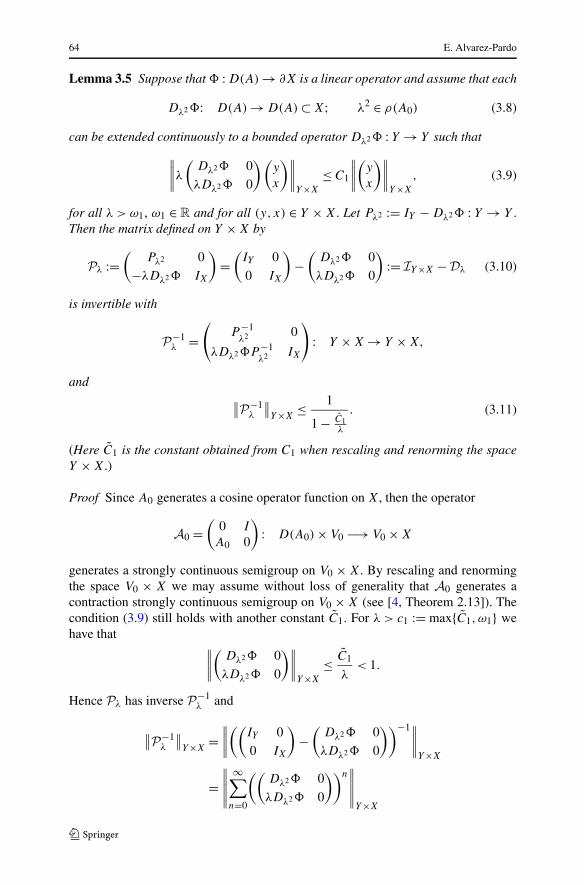
Lemma 3.5 Suppose that � : D(A) → ∂X is a linear operator and assume that each
Dλ2�: D(A) → D(A) ⊂ X; λ2 ∈ ρ(A0) (3.8)
can be extended continuously to a bounded operator Dλ2� : Y → Y such that∥∥∥∥λ
(Dλ2� 0
λDλ2� 0
)(y
x
)∥∥∥∥Y×X
≤ C1
∥∥∥∥(
y
x
)∥∥∥∥Y×X
, (3.9)
for all λ > ω1, ω1 ∈ R and for all (y, x) ∈ Y × X. Let Pλ2 := IY − Dλ2� : Y → Y .Then the matrix defined on Y × X by
Pλ :=(
Pλ2 0
−λDλ2� IX
)=
(IY 0
0 IX
)−
(Dλ2� 0
λDλ2� 0
):= IY×X − Dλ (3.10)
is invertible with
P −1λ =
(P −1
λ2 0
λDλ2�P −1λ2 IX
): Y × X → Y × X,
and ∥∥P −1λ
∥∥Y×X
≤ 1
1 − C1λ
. (3.11)
(Here C1 is the constant obtained from C1 when rescaling and renorming the spaceY × X.)
Proof Since A0 generates a cosine operator function on X, then the operator
A0 =(
0 I
A0 0
): D(A0) × V0 −→ V0 × X
generates a strongly continuous semigroup on V0 × X. By rescaling and renormingthe space V0 × X we may assume without loss of generality that A0 generates acontraction strongly continuous semigroup on V0 × X (see [4, Theorem 2.13]). Thecondition (3.9) still holds with another constant C1. For λ > c1 := max{C1,ω1} wehave that ∥∥∥∥
(Dλ2� 0
λDλ2� 0
)∥∥∥∥Y×X
≤ C1
λ< 1.
Hence Pλ has inverse P −1λ and
∥∥P −1λ
∥∥Y×X
=∥∥∥∥((
IY 0
0 IX
)−
(Dλ2� 0
λDλ2� 0
))−1∥∥∥∥Y×X
=∥∥∥∥∥
∞∑n=0
((Dλ2� 0
λDλ2� 0
))n∥∥∥∥∥
Y×X

Perturbing the boundary conditions of the generator of a cosine family 65
≤∞∑
n=0
∥∥∥∥(
Dλ2� 0
λDλ2� 0
)∥∥∥∥n
Y×X
≤ 1
1 − C1λ
.
Thus for λ sufficiently large
∥∥P −1λ
∥∥Y×X
≤ 1
1 − C1λ
. (3.12)
On the other hand, it can be verified that
P −1λ =
(P −1
λ2 0
λDλ2�P −1λ2 IX
): Y × X → Y × X.
Therefore the conclusion of the lemma follows. �
The next theorem is the first main result of this section.
Theorem 3.6 Suppose that the hypothesis in Lemma 3.5 hold. If V0 = Y and theoperator (A0,D(A0)) generates a cosine operator function with phase space V0 ×X,then the operator (A�,D(A�)) also generates a cosine operator function with thesame phase space V� × X where V� = Y .
Proof Let
A� =(
0 IY
A� 0
): D(A�) × Y −→ Y × X, Pλ :=
(Pλ2 0
−λDλ2� IX
).
Note that A� = A0 when � = 0. Then for f ∈ D(A�), and g ∈ Y , we have
(λ − A0)Pλ
(f
g
)=
(λ −IY
−A0 λ
)(Pλ2 0
−λDλ2� I
)(f
g
)
=(
λ −IY
−A0 λ
)(Pλ2f
−λDλ2�f + g
)
=(
λPλ2f + λDλ2�f − IY g
−A0Pλ2f − λ2Dλ2�f + λg
)
=(
λf − g
−A�f + λg
)
=(
λ −IY
−A� λ
)(f
g
)
= (λ − A�)
(f
g
),
66 E. Alvarez-Pardo
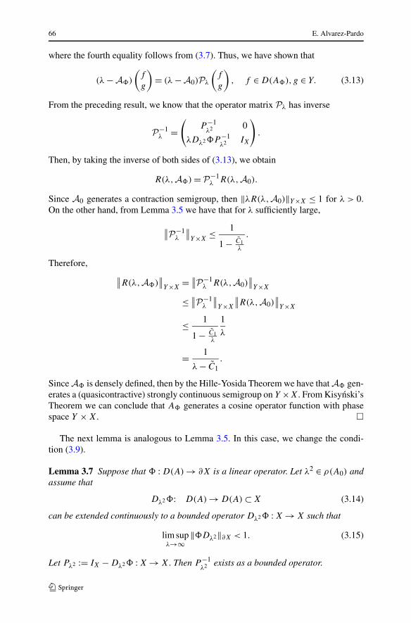
where the fourth equality follows from (3.7). Thus, we have shown that
(λ − A�)
(f
g
)= (λ − A0)Pλ
(f
g
), f ∈ D(A�),g ∈ Y. (3.13)
From the preceding result, we know that the operator matrix Pλ has inverse
P −1λ =
(P −1
λ2 0
λDλ2�P −1λ2 IX
).
Then, by taking the inverse of both sides of (3.13), we obtain
R(λ, A�) = P −1λ R(λ, A0).
Since A0 generates a contraction semigroup, then ‖λR(λ, A0)‖Y×X ≤ 1 for λ > 0.On the other hand, from Lemma 3.5 we have that for λ sufficiently large,
∥∥P −1λ
∥∥Y×X
≤ 1
1 − C1λ
.
Therefore, ∥∥R(λ, A�)∥∥
Y×X= ∥∥P −1
λ R(λ, A0)∥∥
Y×X
≤ ∥∥P −1λ
∥∥Y×X
∥∥R(λ, A0)∥∥
Y×X
≤ 1
1 − C1λ
1
λ
= 1
λ − C1.
Since A� is densely defined, then by the Hille-Yosida Theorem we have that A� gen-erates a (quasicontractive) strongly continuous semigroup on Y ×X. From Kisynski’sTheorem we can conclude that A� generates a cosine operator function with phasespace Y × X. �
The next lemma is analogous to Lemma 3.5. In this case, we change the condi-tion (3.9).
Lemma 3.7 Suppose that � : D(A) → ∂X is a linear operator. Let λ2 ∈ ρ(A0) andassume that
Dλ2�: D(A) → D(A) ⊂ X (3.14)
can be extended continuously to a bounded operator Dλ2� : X → X such that
lim supλ→∞
‖�Dλ2‖∂X < 1. (3.15)
Let Pλ2 := IX − Dλ2� : X → X. Then P −1λ2 exists as a bounded operator.
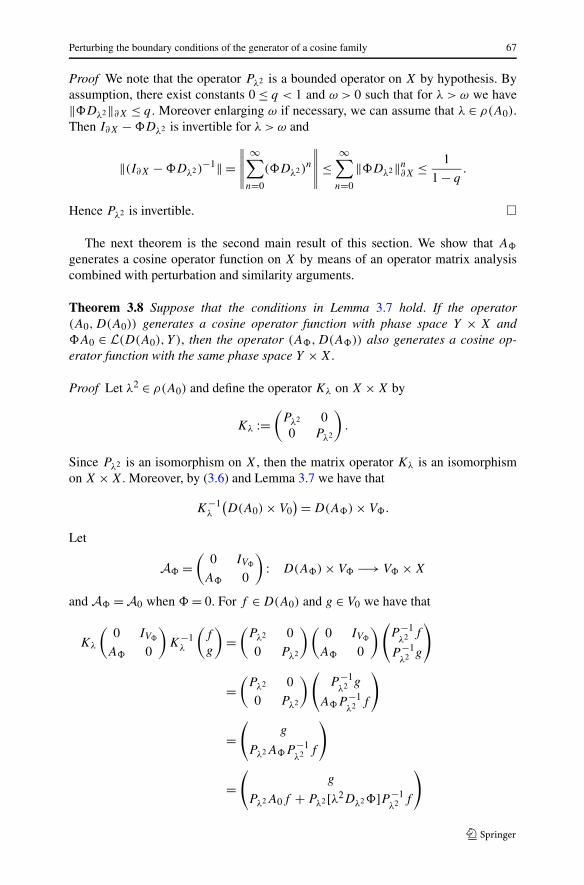
Perturbing the boundary conditions of the generator of a cosine family 67
Proof We note that the operator Pλ2 is a bounded operator on X by hypothesis. Byassumption, there exist constants 0 ≤ q < 1 and ω > 0 such that for λ > ω we have‖�Dλ2‖∂X ≤ q . Moreover enlarging ω if necessary, we can assume that λ ∈ ρ(A0).Then I∂X − �Dλ2 is invertible for λ > ω and
‖(I∂X − �Dλ2)−1‖ =
∥∥∥∥∥∞∑
n=0
(�Dλ2)n
∥∥∥∥∥ ≤∞∑
n=0
‖�Dλ2‖n∂X ≤ 1
1 − q.
Hence Pλ2 is invertible. �
The next theorem is the second main result of this section. We show that A�
generates a cosine operator function on X by means of an operator matrix analysiscombined with perturbation and similarity arguments.
Theorem 3.8 Suppose that the conditions in Lemma 3.7 hold. If the operator(A0,D(A0)) generates a cosine operator function with phase space Y × X and�A0 ∈ L(D(A0), Y ), then the operator (A�,D(A�)) also generates a cosine op-erator function with the same phase space Y × X.
Proof Let λ2 ∈ ρ(A0) and define the operator Kλ on X × X by
Kλ :=(
Pλ2 00 Pλ2
).
Since Pλ2 is an isomorphism on X, then the matrix operator Kλ is an isomorphismon X × X. Moreover, by (3.6) and Lemma 3.7 we have that
K−1λ
(D(A0) × V0
) = D(A�) × V�.
Let
A� =(
0 IV�
A� 0
): D(A�) × V� −→ V� × X
and A� = A0 when � = 0. For f ∈ D(A0) and g ∈ V0 we have that
Kλ
(0 IV�
A� 0
)K−1
λ
(f
g
)=
(Pλ2 0
0 Pλ2
)(0 IV�
A� 0
)(P −1
λ2 f
P −1λ2 g
)
=(
Pλ2 0
0 Pλ2
)(P −1
λ2 g
A�P −1λ2 f
)
=(
g
Pλ2A�P −1λ2 f
)
=(
g
Pλ2A0f + Pλ2 [λ2Dλ2�]P −1λ2 f
)
68 E. Alvarez-Pardo
=(
g
A0f + Dλ2�(λ2 − A0)f
)
=(
0 IV0
A0 0
)(f
g
)+
(0 0
Dλ2�(λ2 − A0) 0
)(f
g
).
Hence, we have shown that KλA�K−1λ = A0 + B, where B := ( 0 0
Dλ2�(λ2−A0) 0
).
Since �A0 ∈ L(D(A0), Y ), then the operator B := Dλ2�(λ2 − A0) ∈ L(D(A0), Y ).
Therefore, the operator matrix B ∈ L(D(A0) × Y). Since A0 generates a C0-semigroup on V0 ×X, then A0 + B also generates a C0-semigroup on V0 ×X; henceKλA�K−1
λ also generates a C0-semi-group on P −1λ2 (V0 × X) = V� × X. �
3.4 The Case V0 = Xα := (X,D(A0))0α,∞ and X0 = X
In this next section, we will analyze the case when the space Y is replaced bythe real interpolation space Xα = (X,D(A0))
0α,∞ with 0 < α ≤ 1
2 . Recall from [7,Lemma 3.6] that
(X,D(A0)
)0α,∞ =
{x ∈ X : lim
t→0t−2α
(C0(t)x − x
) = 0}
and
‖x‖α := sup0<t≤1
t−2α‖C0(t)x − x‖X,
where C0(t) is the cosine family generated by A0.First of all, we recall some results related to the estimate of the resolvent R(λ2,A0)
considered as operator from Xα to Xβ . Let λ2 ∈ ρ(A0). By using λ2 instead λ in [6,Lemmas 2.2, 2.3, 2.4], we obtain the following three lemmas.
Lemma 3.9 Let α ∈ (0, 12 ). The following assertions are equivalent.
(a) limλ→∞ λ2α‖Dλ2z‖α = 0 for all z ∈ ∂X;(b) D(A) ⊂ Xα and the inclusion is continuous;(c) ker(μ2 − A) ⊂ Xα for some μ2 ∈ ρ(A0).
If α,β ∈ [0, 12 ], then the operator R(λ2,A0) is considered as an operator from Xα
to Xβ and we denote its norm by ‖R(λ2,A0)‖αβ .
Lemma 3.10 The following assertions hold:
(a) If 0 ≤ α ≤ β ≤ 12 then ‖R(λ2,A0)‖α
β = O(λ2β−2α−2) for λ → ∞;
(b) If 0 ≤ β ≤ α < 12 then ‖λ2R(λ2,A0) − I‖α
β = O(λ2β−2α) for λ → ∞.
Lemma 3.11 Assume that 0 ≤ α ≤ β ≤ 12 and D(A) ⊂ Xα . Let λ2 ∈ ρ(A0). Then
the norm of the Dirichlet map Dλ2 considered as mapping from ∂X in Xβ satisfies
‖Dλ2‖β = O(λ2(β−α)
), for λ → ∞. (3.16)
Perturbing the boundary conditions of the generator of a cosine family 69
We present now a version of Lemma 3.5 for the space Xα for 0 < α ≤ 12 . For this,
we require that � is a compact operator.
Lemma 3.12 Let λ2 ∈ ρ(A0) and � : Xα → ∂X be a compact operator. Then‖λDλ2�‖α
α = O(1) if α = 12 ; and if 0 < α < 1
2 we have ‖Dλ2�‖αα → 0 as λ → ∞. In
particular, the operator Pλ2 := IXα − Dλ2� is invertible for λ large.
Proof For simplicity we assume that 0 ∈ ρ(A0). By taking α = β in part (b) ofLemma 3.10 we have that ‖λ2R(λ2,A0) − I‖α
α = O(1) for λ sufficiently large. Letx ∈ D(A0). Using Lemma 3.11, we get that∥∥(
λ2R(λ2,A0
) − I)x∥∥
α= ∥∥(
λ2R(λ2,A0
) − I)A−1
0 A0x∥∥
α
≤ ∥∥(λ2R
(λ2,A0
) − I)A−1
0
∥∥0α‖A0x‖X
= ∥∥R(λ2,A0
)∥∥0α‖A0x‖X = O
(λ2α−2).
Since D(A0) is dense in Xα , we conclude that∥∥(λ2R
(λ2,A0
) − I)x∥∥
α= O
(λ2α−2), for all x ∈ Xα. (3.17)
Let z ∈ ∂X. Then by (3.3) we obtain that
‖Dλ2z‖ = ∥∥(λ2R
(λ2,A0
) − I)D0z
∥∥α
= O(λ2α−2).
We consider two cases. First, suppose that α = 12 . It follows from the preceding
equation that ‖λDλ2z‖αα = O(1). Since � is compact, we have that ‖λDλ2�‖α
α =O(1) for λ sufficiently large. Next, let 0 < α < 1
2 . From (3.17) we obtain that(λ2R(λ2,A0) − I ) → 0 as λ → ∞ in the topology of uniform convergence on com-pact subsets of Xα . Since bounded linear operators map relatively compact sets ontorelatively compact ones, we have
‖Dλ2z‖ = ∥∥(λ2R
(λ2,A0
) − I)D0z
∥∥α
→ 0,
for z in relatively compact sets. Since � is assumed to be compact, it follows that
‖Dλ2�z‖ = ∥∥(λ2R
(λ2,A0
) − I)D0�z
∥∥α
→ 0,
on the unit ball of Xα as λ → ∞. This means that ‖Dλ2�‖αα → 0 as λ → ∞. Hence
IXα − Dλ2� is invertible for λ large. �
The following lemma is similar to the Lemma 3.5. In this case, the compactnessof � plays an important role for the applications.
Lemma 3.13 Let λ2 ∈ ρ(A0) and � : X 12
→ ∂X be a compact operator. Assume that
‖λ2Dλ2�y‖X ≤ K‖y‖X 12
for some K > 0 and for λ sufficiently large. Then
∥∥∥∥λ
(Dλ2� 0
λDλ2� 0
)(y
x
)∥∥∥∥X 1
2×X
≤ C
∥∥∥∥(
y
x
)∥∥∥∥X 1
2×X
(3.18)
70 E. Alvarez-Pardo
for all (y, x) ∈ X 12× X. Moreover, for Pλ2 := IX 1
2− Dλ2� : X 1
2→ X 1
2we have that
the matrix defined on X 12× X
Pλ :=(
Pλ2 0
−λDλ2� IX
)=
(IX 1
20
0 IX
)−
(Dλ2� 0
λDλ2� 0
):= IX 1
2×X − Dλ (3.19)
is invertible with
P −1λ =
(P −1
λ2 0
λDλ2�P −1λ2 IX
): X 1
2× X → X 1
2× X,
and ∥∥P −1λ
∥∥X 1
2×X
≤ 1
1 − C1λ
(3.20)
(Here C1 is the constant obtained from C1 when rescaling and renorming the spaceX 1
2× X.)
Proof Since � is compact, the preceding result gives that ‖λDλ2�‖1212
= O(1) for
λ sufficiently large. Then there exists C1 such that ‖λDλ2�y‖ 12
≤ C1‖y‖ 12. On the
other hand, by hypothesis we have that ‖λ2Dλ2�y‖X ≤ K‖y‖X 12
. In summary,
‖λDλ2�y‖ 12
≤ C1‖y‖ 12
and ‖λ2Dλ2�y‖X ≤ K‖y‖X 12
(3.21)
for all y ∈ X 12
and λ sufficiently large. Thus by (3.21) we obtain that
∥∥∥∥λ
(Dλ2� 0
λDλ2� 0
)(y
x
)∥∥∥∥X 1
2×X
=∥∥∥∥λ
(Dλ2�y
λDλ2�y
)∥∥∥∥X 1
2×X
= ‖λDλ2�y‖ 12+ ‖λ2Dλ2�y‖X
≤ C1‖y‖ 12+ K‖y‖ 1
2
≤ C‖y‖ 12
≤ C‖y‖ 12+ C‖x‖X
= C
∥∥∥∥(
y
x
)∥∥∥∥X 1
2×X
;
for λ sufficiently large. The remaining of the proof can be obtained easily by makinga simple modification of the proof of the Lemma 3.5 �
The next theorem is analogous to Theorem 3.6. The proof is essentially the sameand is therefore omitted. One has to change only the phase space.
Perturbing the boundary conditions of the generator of a cosine family 71
Theorem 3.14 Assume the hypothesis in the Lemma 3.13. If V0 = X 12
and the opera-
tor (A0,D(A0)) generates a cosine operator function with phase space V0 ×X, thenthe operator (A�,D(A�)) also generates a cosine operator function with the samephase space V� × X where V� = X 1
2.
Remark 3.15 For 0 < α < 12 we know from Lemma 3.12 that ‖Dλ2�‖α
α → 0 asλ → ∞. But this could imply that the resolvent of A� goes to zero rapidly; which isa contradiction. Thus � compact is not very good in this case. However, we obtainsimilar results to the Lemma 3.5 and Theorem 3.6 if we replace Y by Xα in theirstatements.
4 Multiplicative perturbation
In this section we obtain an abstract generation result by using multiplicative pertur-bations. This kind of results has been developed by Piskarev and Shaw in [13].
Throughout this section we consider the following framework.
(1) X,Y, ∂X are three Banach spaces;(2) A : D(A) ⊂ X → X is closed, densely defined linear operator (the “maximal
operator”);
(3) D(A) ⊂ Y ↪→ X, D(A)‖·‖Y = Y, and Y
‖·‖X = X;(4) L : [D(A)] → ∂X a linear surjective operator (here [D(A)] is a Banach space
with the graph norm);(5) V0 is a Banach space such that V0 ↪→ Y ;(6) L can be extended continuously to Y with ker(L) = V0;(7) the restriction A0 := A |ker(L) generates a cosine function operator on X with
phase space V0 × X;(8)
(AL
) : [D(A)]L → X × ∂X is closed. Here [D(A)]L is a Banach space with thenorm ‖u‖[D(A)]L := ‖u‖X + ‖Au‖X + ‖Lu‖∂X .
The following lemma is a direct consequence of multiplicative perturbation ofcosine functions results.
Lemma 4.1 Let A0 generates a cosine operator function with associated phasespace V0 × X. Let ε > 0 be sufficiently small. Assume that
‖Dλ‖L(∂X,X) = O(|λ|−ε
), |λ| → ∞, Reλ > 0 (4.1)
and ∫ 1
0‖�A0S(s,A0)f ‖∂X ds ≤ M‖f ‖X (4.2)
holds for all f ∈ D(A0) and some M > 0. Then A0 − Dλ�A0 = (I − Dλ�)A0 =:PλA0 generates a cosine operator function with associated phase space V0 × X.
72 E. Alvarez-Pardo
Proof Combining (4.1) and (4.2) we obtain that∫ 1
0‖Dλ�A0S(s,A0)f ‖∂Xds ≤ q‖f ‖X, for all f ∈ D(A0),
and some q < 1. By taking R := I − Dλ� and B := R − I = −Dλ� in [13, Theo-rem 2.6] the conclusion of the lemma follows. �
Remark 4.2 The assumption on the decay of the norm of the Dirichlet operator thatappears in (4.1) is in particular satisfied whenever D(A) is contained in any complexinterpolation space Xε := [D(A0,X)]ε , 0 < ε < 1, cf. [6, Lemma 2.4]. Such interpo-lation spaces are well defined, since in particular A0 generates an analytic semigroup.
Theorem 4.3 Assume the general assumptions of the framework. Let � : X → ∂X
be a bounded operator and suppose that the conditions (4.1) and (4.2) hold. Then(A�,D(A�)) generates a cosine operator function.
Proof Let λ ∈ ρ(A0). By Lemma 4.1 we have that ((I − Dλ�)A0,D(A0)) =(PλA0,D(A0)) generates a cosine operator function. By [5, Lemma 1.4] note that
D(A�) = {f ∈ X : (I − Dλ�)f ∈ D(A0)
}.
We claim that D(A�) is dense in X. Indeed, since the operator Pλ := I − Dλ� isbounded on X and (A0,D(A0)) generates a cosine operator function, and by hypoth-esis (PλA0,D(A0)) also generates a cosine operator function; then, from [1] bothgenerate analytic semigroups, thus from the proof of [12, Theorem 4.4] we have thatD(A�) is dense in X. Now,
A0(I − Dλ�)f = A(I − Dλ�)f
= Af − ADλ�f
= Af − λDλ�f
= A�f − λDλ�f,
therefore
A�f = A0(I − Dλ�)f + λDλ�f = A0Pλf + λDλ�f,
for all f ∈ D(A�). Finally, since PλA0 generates a cosine operator function, thenfrom [13, Proposition 2.1] we have that A0Pλ also generates a cosine operator func-tion. On the other hand, observe that λDλ� is bounded on X, so by [4, Theorem 8.5]we have that A� generates a cosine operator function. �
5 Examples and closing remarks
In the following section we discuss some applications and remarks of the previousresults. As an application of the first theorem, we give some generation result for a

Perturbing the boundary conditions of the generator of a cosine family 73
realization of the Laplace operator with nonlocal Wentzell boundary conditions onC[0,1].
Example 5.1 Let Au = �u = u′′;D(A) = C2[0,1];Y := C1[0,1];X := C[0,1],∂X = C
2;� : C1[0,1] → C2;L : C2[0,1] → C
2 defined by
�u :=(
β0u′(0) + γ0u(0) + σ1u(1)
β1u′(1) + γ1u(1) + σ0u(0)
); Lu :=
(α0u
′′(0)
α1u′′(1)
),
where αi,βi, γi, σi ∈ C and αi �= 0 for all i = 0,1. Note that ker(L) = {u ∈ C2[0,1] :u′′(0) = u′′(1) = 0} and A0u = Au = u′′. Thus A0 = �W is the Laplace operatorwith Wentzell boundary conditions on C[0,1]. It is known that this operator gener-ates a cosine operator function with phase space C1[0,1]) × C[0,1] (see [2]). TheLaplacian with non local Wentzell-Robin boundary conditions on C[0,1] is definedby D(ANW,∞) := {u ∈ C2[0,1] : αiu
′′(i) + βiu′(i) + γiu(i) + σ1−iu(1 − i) = 0, i =
0,1}; ANWu := u′′.Then (A�,D(A�)) = (�NW,∞,D(�NW,∞)). Observe that for u ∈ C1[0,1] we
have
‖�u‖C2 = M1(∣∣u(0)
∣∣ + ∣∣u(1)∣∣) + M2
(∣∣u′(0)∣∣ + ∣∣u′(1)
∣∣) ≤ M3‖u‖C1[0,1]; (5.1)
where M1 := max{|γ0 +σ0|, |γ1 +σ1|}, M2 := max{|β0|, |β1|} and M3 := max{2M1,
2M2}. Let (DW)λ2 be the Dirichlet operator corresponding to the operator A0 = �W .Solving the system that appears in the Lemma 3.2 one obtains that
(DW)λ2(a, b)(x) = b sinhλx + a sinhλ(1 − x)
λ2 sinhλ, (a, b) ∈ C
2, x ∈ [0,1]
for λ > 0. The inequality (3.9) follows from the maximum principle. Hence from thepreceding theorem, we obtain that the operator �NW,∞ generates a cosine operatorfunction on C[0,1] with phase space C1[0,1] × C[0,1].
Remark 5.2 Theorem 3.6 cannot be applied to A0 = �N, the Laplacian with Neu-mann boundary conditions on Lp(0,1) because the estimate ‖λDλ2�‖X ≤ C doesnot hold.
Example 5.3 Let X := Lp(0,1), Y := W 1,p(0,1) and D(A) := W 2,p(0,1). Considerthe Laplace operator �u := u′′. We define the linear operators � : Lp(0,1) → C
2,L : W 2,p(0,1) → C
2 by
�u :=(∫ 1
0 k(0, y)u(y)dy∫ 10 k(1, y)u(y)dy
); Lu :=
(u′(0)
u′(1)
),
where k := (k(0, ·), k(1, ·)) : [0,1] → C is twice differentiable. Since ker(L) = {u ∈W 2,p(0,1) : u′(0) = u′(1) = 0} and A0u = Au = u′′ then A0 = �N is the Laplaceoperator with Neumann boundary conditions on Lp(0,1). Then A0 generates a cosineoperator function on Lp(0,1) with phase space W 1,p(0,1) × Lp(0,1) (see [8]).
74 E. Alvarez-Pardo
On the other hand, integration by parts gives
‖�A0u‖ =∥∥∥∥∥(∫ 1
0 k(0, y)u′′(y)dy∫ 10 k(1, y)u′′(y)dy
)∥∥∥∥∥C2
≤ M‖u′‖L1(0,1) ≤ ‖u‖W 1,p(0,1);
u ∈ D(A0).
Now, the Dirichlet operator corresponding to the Laplacian with Neumann boundaryconditions is given by
(DN)λ2(a, b)(x) = b coshλx − a coshλ(1 − x)
λ sinhλ, (a, b) ∈ C
2, x ∈ [0,1].
Then, it can be verified that limλ→∞ ‖�Dλ2‖ = 0 < 1.Since � ∈ L(X, ∂X), then Dλ2� is continuous from X to ∂X. Hence, all the
hypothesis in Lemma 3.7 and Theorem 3.8 hold. Thus the operator A� := u′′ withdomain D(A�) := {u ∈ W 2,p(0,1) : u′(i) = ∫ 1
0 k(i, y)u(y)dy; i = 0,1} generates acosine operator function on X with phase space W 1,p(0,1) × Lp(0,1).
Acknowledgements The author wish to express their gratitude to V. Keyantuo, C. Lizama andM. Warma for valuable suggestions concerning the preparation of this manuscript.
References
1. Arendt, W., Batty, C., Hieber, M., Neubrander, F.: Vector-Valued Laplace Transforms and CauchyProblems. Birkhäuser, Basel (2001)
2. Bátkai, A., Engel, K.-J.: Abstract wave equations with generalized Wentzell boundary conditions.J. Differ. Equ. 207, 1–20 (2004)
3. Chill, R., Keyantuo, V., Warma, M.: Generation a cosine families on Lp(0,1) by elliptic operatorswith Robin boundary conditions. In: Functional Analysis and Evolutions Equations, Günter LumerVolume, pp. 113–130 (2007)
4. Goldstein, J.: Semigroups of Linear Operators and Applications. Oxford University Press, New York(1985)
5. Greiner, G.: Perturbing the boundary conditions of a generator. Houst. J. Math. 13, 213–229 (1987)6. Greiner, G., Kuhn, K.: Linear and semilinear boundary conditions: the analytic case. In: Lecture Notes
in Pure and Applied Mathematics, vol. 135, pp. 193–211 (1991)7. Hoppe, R.: Interpolation of cosine operator functions. Ann. Mat. Pura Appl. 136, 183–212 (1984)8. Keyantuo, V., Warma, M.: The wave equation on Lp spaces. Semigroup Forum 71, 73–92 (2005)9. Keyantuo, V., Warma, M.: The wave equation with Wentzell-Robin boundary conditions on Lp
spaces. J. Differ. Equ. 229, 680–697 (2006)10. Kisynski, J.: On cosine operator functions and one-parameter groups operators. Stud. Math. 44, 93–
105 (1969)11. Mugnolo, D.: Operator matrices as generators of cosine operator functions. Integral Equ. Oper. Theory
54, 441–464 (2006)12. Nickel, G.: A new look at boundary perturbations of generators. Electron. J. Differ. Equ. 95, 1–14
(2004)13. Piskarev, S., Shaw, S.-Y.: Perturbation and comparison of cosine operator functions. Semigroup Fo-
rum 51, 225–246 (1995)14. Xiao, T.-J., Liang, J.: Second order differential operators with Feller-Wentzell type boundary condi-
tions. J. Funct. Anal. 254, 1467–1486 (2008)


