
Perturbation Theory for Evaluation Algorithms of ...€¦ · Perturbation Theory for Evaluation...
39
mathematics of computation volume 37, number 156 OCTOBER 1981 Perturbation Theory for Evaluation Algorithms of Arithmetic Expressions By F. Stummel Abstract. The paper presents the theoretical foundation of a forward error analysis of numerical algorithms under data perturbations, rounding error in arithmetic floating-point operations, and approximations in 'built-in' functions. The error analysis is based on the linearization method that has been proposed by many authors in various forms. Fundamen- tal tools of the forward error analysis are systems of linear absolute and relative a priori and a posteriori error equations and associated condition numbers constituting optimal bounds of possible accumulated or total errors. Derivations, representations, and properties of these condition numbers are studied in detail. The condition numbers enable simple general, quantitative definitions of numerical stability, backward analysis, well- and ill-conditioning of a problem and an algorithm. The well-known illustration of algorithms and their linear error equations by graphs is extended to a method of deriving condition numbers and associated bounds. For many algorithms the associated condition numbers can be de- termined analytically a priori and be computed numerically a posteriori. The theoretical results of the paper have been applied to a series of concrete algorithms, including Gaussian elimination, and have proved to be very effective means of both a priori and a posteriori error analysis. Introduction. Evaluation algorithms are defined by finite sequences F = iF0, . . . , Fn) of input operations, evaluations of 'built-in' functions, and arithmetic operations for determining sequences u = (m0, . . . , u„) of input data, intermediate and final results in the form (1) u, = F,iu), t = 0, . . ., n. It is presupposed in the following that F0 is a constant function and the function values Ftix) depend on x0, . . . , x,_x but not on x„ . . . , xn for t = 1, . . ., n. Under perturbations, an evaluation algorithm yields approximations t>, of u, that can be written in the form (2) vt - (1 + e,)F,iv), t = 0,...,n. The so-called local errors e, are the relative errors of the data input, function evaluation, or rounding in the arithmetic floating-point operation in step t of the algorithm. We shall assume that the local errors are bounded by \e,\ < ytt\ for / = 0, . . . , n, where y, are suitable nonnegative weights and 17 is an accuracy constant. Received June 12, 1979; revised November 26, 1979 and August 27, 1980. 1980 Mathematics Subject Classification. Primary 65G05. Key words and phrases. Rounding error analysis, evaluation algorithms, a priori and a posteriori error estimates, condition numbers, linear error equations, graphs. © 1981 American Mathematical Society 0025-S718/81/0000-0164/$10.75 435 License or copyright restrictions may apply to redistribution; see http://www.ams.org/journal-terms-of-use
Transcript of Perturbation Theory for Evaluation Algorithms of ...€¦ · Perturbation Theory for Evaluation...

mathematics of computationvolume 37, number 156OCTOBER 1981
Perturbation Theory for Evaluation Algorithms
of Arithmetic Expressions
By F. Stummel
Abstract. The paper presents the theoretical foundation of a forward error analysis of
numerical algorithms under data perturbations, rounding error in arithmetic floating-point
operations, and approximations in 'built-in' functions. The error analysis is based on the
linearization method that has been proposed by many authors in various forms. Fundamen-
tal tools of the forward error analysis are systems of linear absolute and relative a priori and
a posteriori error equations and associated condition numbers constituting optimal bounds
of possible accumulated or total errors. Derivations, representations, and properties of these
condition numbers are studied in detail. The condition numbers enable simple general,
quantitative definitions of numerical stability, backward analysis, well- and ill-conditioning
of a problem and an algorithm. The well-known illustration of algorithms and their linear
error equations by graphs is extended to a method of deriving condition numbers and
associated bounds. For many algorithms the associated condition numbers can be de-
termined analytically a priori and be computed numerically a posteriori. The theoretical
results of the paper have been applied to a series of concrete algorithms, including Gaussian
elimination, and have proved to be very effective means of both a priori and a posteriori
error analysis.
Introduction. Evaluation algorithms are defined by finite sequences F =
iF0, . . . , Fn) of input operations, evaluations of 'built-in' functions, and arithmetic
operations for determining sequences u = (m0, . . . , u„) of input data, intermediate
and final results in the form
(1) u, = F,iu), t = 0, . . ., n.
It is presupposed in the following that F0 is a constant function and the function
values Ftix) depend on x0, . . . , x,_x but not on x„ . . . , xn for t = 1, . . ., n.
Under perturbations, an evaluation algorithm yields approximations t>, of u, that
can be written in the form
(2) vt - (1 + e,)F,iv), t = 0,...,n.
The so-called local errors e, are the relative errors of the data input, function
evaluation, or rounding in the arithmetic floating-point operation in step t of the
algorithm. We shall assume that the local errors are bounded by \e,\ < ytt\ for
/ = 0, . . . , n, where y, are suitable nonnegative weights and 17 is an accuracy
constant.
Received June 12, 1979; revised November 26, 1979 and August 27, 1980.
1980 Mathematics Subject Classification. Primary 65G05.
Key words and phrases. Rounding error analysis, evaluation algorithms, a priori and a posteriori error
estimates, condition numbers, linear error equations, graphs.
© 1981 American Mathematical Society
0025-S718/81/0000-0164/$10.75
435
License or copyright restrictions may apply to redistribution; see http://www.ams.org/journal-terms-of-use

436 F. STUMMEL
In vector notation, (1), (2) may be written u = Fiu), v = Fiv) + d, using the
residual vector d with the components dt = -v,e¡ and e't = -ejil + et). By intro-
ducing the mapping A = / — F, (1), (2) become
(3) Au = 0, Av = d.
Thus, the error analysis of an evaluation algorithm is a perturbation theory of the
functional equation Au = 0 with respect to perturbations of the right-hand side. By
Taylor's formula at the point u, the absolute a priori error Au = v — u satisfies the
relation iA'u)Au + R = d, where R is a remainder term of order 0(||Au||2).
Neglecting terms of second order in ||Au|| and tj gives iA'u)Au = Jue, where
Ju = diag(w0, .. ., u„). In the a posteriori error analysis, one uses Taylor's formula
at the point v and obtains the relation iA'v)Av = Jve' for the error Av = u — v.
The solutions s of the associated systems of linear error equations
(4) iA'u)s = Jue, or iA'v)s = Jve',
then yield approximations of the absolute errors Au or Av. Correspondingly,
approximations r of the relative errors Pu = J~xAu or Pv = J~xAv are obtained
from the systems of linear error equations
(5) J-\A'u)Jur = e, or J;\A'v)Jj = e'.
The procedure, described above, is analogous to the derivation of difference
approximations of a differential equation; the role of truncation errors is played by
remainder terms 0(||Au||2), 0(tj2) here. Note that the linear error equations can
also be derived simply from the exact error equations in Section 1.1 by neglecting
terms of second order in the errors and replacing the absolute and relative errors of
u, v by s and r.
The subject of the paper is a study of the structure of the mapping A and its
Fréchet-derivative A'w, the derivation and proof of error representations of the
form
(6) Aw, - s, + 0,(t,2), Pw, = r, + 0,iv2),
where s, r are the solutions of (4), (5), and associated optimal error estimates
(7) |Aw,| < <7,t, + O/t,2), |/V,| < p,7, + 0,(ij2),
a detailed analysis of the remainder terms in (6), (7) and of the properties of the
optimal constants o„ pt. In (6), (7), one chooses w = u in an a priori and w = v in
an a posteriori error analysis. The components st, r, of s, r are linear forms in the
local errors e = (e0, . . . , en), and the bounds a,n, p,n are associated norms,
specified by the error distribution, \et\ < y,t\, of these linear forms. The constants
a,, p, are the weighted absolute and relative, a priori and a posteriori condition
numbers.
Particular attention is paid in the following to the simultaneous treatment of
absolute and relative, a priori and a posteriori errors as well as to readily accessible
presentations of the coefficients and inhomogeneous terms of the associated error
equations, of condition numbers, weights, and so on, in all four cases. For, in
applications to concrete examples it is seen that for some algorithms the systems of
linear absolute error equations, for others the systems of linear relative error
equations, are easier to handle. The general theoretical rounding error analysis of
License or copyright restrictions may apply to redistribution; see http://www.ams.org/journal-terms-of-use

EVALUATION ALGORITHMS OF ARITHMETIC EXPRESSIONS 437
numerical algorithms uses a priori error representations. In many examples, condi-
tion numbers can be computed numerically a posteriori, that is, together with the
intermediate and final results of the algorithm.
By a suitable choice of the weights in the local error distribution, the behavior of
the algorithm can be studied under data perturbations only, assuming exact
'built-in' functions and arithmetic operations, as well as under rounding errors in
the arithmetic operations and 'built-in' functions only, assuming exact data. The
associated absolute and relative condition numbers are denoted by o,D, aR and pf,
p,R. The data condition numbers of are absolute asymptotic conditions, in the
sense of Rice [15], of ut viewed as a function of the data and thus independent of
the algorithm (see Section 2.1). By Wilkinson [25, 1.36], a problem is said to be
ill-conditioned if small relative errors of the input data can induce great relative
errors of the solution u, of the algorithm. This effect can be formulated quantita-
tively in our terms by ptD » 1. Wilkinson's backward analysis describes the
behavior of the algorithm under rounding errors in the arithmetic operations by
data perturbations. Our results in Section 2.1 show that o,R/o,D = pR /p,° is a
measure for the magnitude of those data perturbations which are necessary and
sufficient in order to represent perturbations by rounding errors in the arithmetic
operations. Bauer's concept (see [4], [5]) of a well-conditioned algorithm for the
computation of u, can be specified by the requirement that pR/p,D is not much
greater than one.
Also, a well-conditioned algorithm can produce numerical results such that not
even the first digit is significant. This happens when the problem is ill-conditioned
and the accuracy tj is too low. The least number of significant digits in a computed
result can be determined by our relative condition numbers p, and the associated
notion of numerical stability. Let data perturbations and rounding errors, within a
given distribution of local errors, be bounded by the accuracy tj0. Then the result v,
is computed under all these perturbations within the relative error bound tj, if the
stability inequality p, < ~qx/-q0 holds. This result follows immediately from (7) for
tj = tj0. For example, choosing tj, = \ and tj0 < l/(2p,) guarantees that at least the
first digit in the computed result v, is accurate in the sense of relative errors. It is
always assumed that remainder terms of the form 0(tj2) are negligible against the
terms of first order in tj.
Evaluation algorithms and their systems of linear error equations may be
illustrated by graphs constituting detailed complete flow diagrams of the functional
dependences between the data, intermediate and final results, as well as exhibiting
the paths of error propagation and the associated error effects along these paths. It
seems that this tool is found for the first time in the book of McCracken-Dorn [11]
who attribute the idea to H. M. King. In essentially the same form Bauer [5],
Brown [7], Linnainmaa [10], and others use graphs in their error analyses. The
matrix elements of the solution operators iA'w)'x, J~xiA'wyxJw can be read from
the weighted graph. In addition, Section 2.3 provides graph theoretic means for
determining condition numbers and associated bounds. For instance, when the
graph of the algorithm is a tree, condition numbers are obtained recurrently by
simple formulae having the same form as those of the condition numbers of the
simplest algorithms in Section 1.1.
License or copyright restrictions may apply to redistribution; see http://www.ams.org/journal-terms-of-use

438 F. STUMMEL
Note that the concepts of condition numbers used, for example, by Wilkinson
[25], Bauer [5], or the well-known condition numbers of matrices, are defined
differently and have other meanings. In the rounding error analysis of a fixed-point
arithmetic, Henrici [8, 16.4] states a system of linear equations for the exact errors
Awr Also the optimality of error bounds, obtained in this way, is observed there.
Linnainmaa [10] studies Taylor expansions of the total errors A«, with respect to
the local errors e0, . . . , e„. In particular, two algorithms for computing the coeffi-
cient matrices of the terms of first and second order in the expansions of the total
errors are presented. We can interpret the first algorithm as a procedure to
compute the rows of the inverse matrix (/I'm)-1 from the matrix F'iu) (see Section
1.3). This algorithm has been described by Larson-Sameh [9] in a somewhat
different context. Bauer [5], Brown [7], and Larson-Sameh [9] use relative or
logarithmic derivatives for obtaining representations of the total relative errors Put.
This method yields first-order approximations of the errors that coincide with the
solutions r, of the system of linear relative a priori error equations (5).
Another way of deriving a priori error representations and estimates of the kind
described above starts from an analysis of the perturbed results t>, viewed as
functions of the local errors e = (e0, . . ., e„). Let v, = G,ie), then u, = G,(0) and,
by Taylor expansion,
(8) Au, = G,'i0)e + 6>,(tj2).
From (4), (6) with w = u, and (8) it follows that s, = G/(0)e for all local errors e
and
(9) 67(0) = ptt(A'u)-%
where pr, denotes the orthogonal projection onto the rth coordinate axis. The
absolute a priori condition numbers thus permit the representation
(10) a, = lim - sup \G,ie) - G,(0)| = ¿i-> + rj tj |e|<yT) ¿=0
dG,yk-
Babuska's stability constants A in [1], [2] are defined in the form of the first
equation in (10). Miller's papers [12], [13] use condition numbers of the kind
defined by the second equation in (10). The associated stability constants 1 +
aR/atD are denoted by Í in [1], [2]. Miller [12], [13] and Miller-Spooner [14] use the
notation p and co, for oR/a,D. When the error analysis is applied to concrete
algorithms, the functional dependence G, of vt on the local errors is, in general,
very complex, so that this approach is limited to small algorithms.
Although the total number of operations, and thus the order of the associated
matrices A'w, becomes very large for many important algorithms, the matrices A'w
are very sparse and highly structured. The directed graph of the functional
dependences of an algorithm and the directed graph of an associated linear system
of error equations are identical. Thus the structure of the system of linear error
equations is, necessarily, related to that of the algorithm. This fact might be the
deeper reason why for many important algorithms, including Gaussian ehmination
of systems of linear algebraic equations, explicit analytical representations of the
solutions of the systems of linear error equations and of the associated condition
numbers can be determined.
License or copyright restrictions may apply to redistribution; see http://www.ams.org/journal-terms-of-use

EVALUATION ALGORITHMS OF ARITHMETIC EXPRESSIONS 439
In a series of papers, surveyed in Section 3, the present error analysis has been
applied to concrete numerical algorithms. The error estimates have been tested by
numerous numerical examples. All these examples have confirmed that the condi-
tion numbers clearly and concisely yield crucial information about the numerical
behavior of the algorithms. The a posteriori condition numbers have proved to be
reliable measures of the magnitude of possible errors.
1. Elements of Error Propagation. The first chapter introduces basic concepts of
the perturbation theory for numerical algorithms. Starting points are representa-
tions and estimates of the errors in elementary arithmetic operations, +, —, X, /,
and 'built-in' functions occurring in the floating-point arithmetic of computers. In
particular, condition numbers are defined for the simplest algorithms, consisting of
the input of one or two operands followed by an arithmetic operation or function
evaluation. It will be seen in Section 2.3 that these condition numbers are also used
in determining condition numbers or associated bounds for general algorithms. In
Section 1.2 the class of algorithms for evaluating arithmetic expressions is defined
and the general form of perturbed algorithms specified in view of typical rounding
error analyses. Further, the general error equations for the solutions of the
perturbed algorithms are derived, and associated estimates for the remainder terms
of Taylor's formula are established. By neglecting remainder terms in the general
error equations, linear error equations arise whose solutions approximate the
absolute and relative a priori and a posteriori errors being of interest. The
algorithm (A) determines uniquely a mapping A in R"+1. It will be shown in
Section 1.3 that the linear error equations are defined by the Fréchet-derivative A'
of A. The solutions of the linear absolute error equations are obtained by means of
the solution operators L = iA'w)'x, and of the relative error equations by L =
J~xiA'w)~xJw. This is in correspondence with the use of so-called relative or
logarithmic derivatives (see Bauer [5], Brown [7]).
1.1. Error Estimates for the Simplest Numerical Algorithms. Given two numbers a,
b and arbitrary approximations a', b' of a, b, the following absolute and relative a
priori and a posteriori errors are defined:
(1)a priori
a posteriori
absolute
Aa = a' — a
Aa' = a — a'
relative
Pa =a — a
Pa' =a — a
In the relative error analysis it will always be assumed that denominators are
different from zero. Let us first state representations of the absolute and relative a
priori errors
(2) A(a ° b) = a' ° V - a ° b, Pia ° b) =a' ° b' — a ° b
a ° b = +, -, X, /,
of sums, differences, products, and quotients under perturbations of the operands
a, b. It is well known that
License or copyright restrictions may apply to redistribution; see http://www.ams.org/journal-terms-of-use

440 F. STUMMEL
A(a ± b) = Aa ± Ab, Pia ± b) = - Pa ± - Pb,c c
(3) Aiab) = bAa + aAb + AaAb, Piab) = Pa + Pb + PaPb,
«<•">' - 7TTa*(a" - !**)■ «•/« - T^ •
where c = a ± b. The numerical computation of a ° b first requires input or
computing of the operands a, b carried out, in general, approximately. The
arithmetic floating-point operations are then applied to approximations of a, b.
Input of a, b gives, for instance, a' = fl(a), b' = fl(6). By fl is meant a function
mapping the real numbers into A/-digit floating-point numbers. Let g denote the
base of the number representation. The floating-point arithmetic thus computes the
approximations
(4) v = fl(a' ° b') = (1 + e)ia' ° b'), \e\ < tj,
of the exact results u = a ° b where ° = + , —, X, / (see Wilkinson [25]). The
floating-point accuracy constant tj is, for example, ¿g~N+x when fl is symmetric
rounding, and g'N+ ' when fl denotes chopping off the mantissae to N digits. Now
A« = v — u = (1 + e)ia' ° b' - a ° b) + e(a ° b),
so that the absolute and relative a priori errors of v have the representations
(5) A« = (1 + e)A(a ° b) + ue, Pu = (1 + e)Pia ° b) + e.
Inserting the above expressions for A(a ° b), Pia ° b) in (3) yields the absolute and
relative a priori error equations.
Analogous representations hold for the absolute and relative a posteriori errors
A(a' ° b') = a ° b — a' ° b',
(6) ,, ,n fl.i-a'oi'/>(a'oA')= -;- , ° = +, -, X, /.
a ° b
They are obtained by interchanging a, b and a', b' in (3). Let us further introduce
the notation
(7) *'=~TT7 l'*-*
Then, evidently,
(8) e + e' + ee' = 0, (1 + e)(l + e') = 1.
Using (4), one has
vAv = u — v = a ° b — a' ° b' — eiá ° b'), a' ° b' =
1 + e'
The absolute and relative a posteriori errors of the approximation v of u can
therefore be written in the form
(9) Av = A(a' o b') + ve', Pv = (1 + e')/V ° V) + e'.
From (3), (9) we obtain absolute and relative a posteriori error equations. Note that
the representation of relative a priori errors turns into that of relative a posteriori
errors when a, b, e, u are interchanged by a', b', e', v.
License or copyright restrictions may apply to redistribution; see http://www.ams.org/journal-terms-of-use

EVALUATION ALGORITHMS OF ARITHMETIC EXPRESSIONS 441
(10)
Next let a real function / of a single variable be given, twice continuously
differentiable in its open domain of definition. Under perturbations of the argu-
ment a, the induced approximations f(a') of fia) have the absolute and relative a
priori errors
/ f\a,a,a'] \Afia) = \l+Jlna) iAajfia)Aa,
using the Hermite generalized divided differences
(11) f[a, a, a'} = f(f/"(a + ¿(a' - a)) ds} dt.
It is presupposed that f\a) and, in the case of relative errors, a and fia) are
different from zero. The above representations are valid for all pairs a, a' such that
the line segment aa' belongs to the domain of definition of/.
In the numerical evaluation of real functions, instead of u = fia) an approxima-
tion of / at a neighboring point a' of a is computed. Let v denote this approxima-
tion. Then
(12) v - (1 + e)j%a'), e = V ~ ffa'> ifia') * 0).
It can be assumed, for example, that elementary 'built-in' functions are computed
by
(13) v = fl(/(a')).
In this case,
(14) e-fí(y)y~y, y=fia'), |«| <,.
In line with (5), (9), one finds the error equations
Au = (1 + e)Afia) + ue, Pu - (1 + e)Pfia) + e,
K ' Av = Afia') + ve', Pv = (1 + e')Pfia') + e',
for the approximations v of u = fia), where e is specified by (12) and herewith e'
by (7). Inserting the representations (10) of Afia) and Pfia) into (15) leads to the
absolute and relative a priori error equations of numerical evaluations of /. Inter-
changing a, ä in (10) and inserting the resulting representations of Afia'), Pfia')
into (15) yields the associated absolute and relative a posteriori error equations.
Again, the relative a priori error equations change to the a posteriori error
equations, and vice versa, when a, e, u are interchanged by a', e', u'.
The simplest numerical algorithms consist of the input of a or a, b followed by
the computation of fia) or a ° b for ° = + , —, X, /. From the above error
equations we can readily deduce associated error estimates. For this purpose, let us
assume that the relative errors Pa, Pb, e+, e_, ... of the input data and arithmetic
floating-point operations +, —, . . . are bounded by
(16) \Pa\ < PaTj, \Pb\ < Patj, \e\ < yrj.
License or copyright restrictions may apply to redistribution; see http://www.ams.org/journal-terms-of-use

442 F. STUMMEL
The absolute errors Aa, Ab then satisfy the estimates
(17) |Aa| < <TaTj, |A6| < a¿Tj, oa = \a\pa, ab = \b\pb.
The constants pa, pb and aa, ob are the relative and absolute a priori condition
numbers of the data a, b. They permit adjusting the bounds to the magnitude of
possible errors of the data approximations a', V. When a, b are results of a
previous numerical computation, in general a', b' have larger errors than input
errors of magnitude tj. Constants pa, pb, oa, ob may be zero when input data are
exact or unperturbed. The weight y can be set equal to zero if the floating-point
operation is performed exactly, for instance, when a loss of significant figures
occurs in subtractions. The error equations (3), (5), (10), (15) entail the absolute and
relative a priori error estimates
(18) |Au| < (1 + 0(t,))otj, \Pu\<il + 0(tj))ptj,
using the following absolute and relative a priori condition numbers of arithmetic
operations and function evaluations:
+ ,-: o = aa + ab + \u\y,
X : o = \b\oa + \a\ob + \u\y,
(19)
P =
a = W\°a + ob + My,
Pa +
P = Pa + Pb + Y>
P = Pa + Pb + Y,
Pb + Y,
a = \f'ia)\aa + \u\y, P =afia)
fia) Pa + y-
Note that always p = a/\u\, u = a ° b for ° = + ,-,X,/ or u = fia). The above
estimates require for divisions that pfcTj < # < 1, and for function evaluations that
\f[a, a, a']\/\f'ia)\ < jt.Let us assume that the a posteriori errors Pa', Pb', e' and Aa', Ab' satisfy
estimates corresponding to (16), (17). From (3), (6), (9), (10), (15) the absolute and
relative a posteriori error estimates
(20) |Ao| < (1 + 0(tj)H, \Pv\ < (1 + G(t,))ptj
follow, where a, p denote the absolute and relative a posteriori condition numbers
(21) /
a = °a + °b + My,
° = \b'\oa + \a'\°b + My,
<>b + My,
p = Pa + Pb + Y,
1a = W\aa +
P = Pa + Pb + Y,
P = Pa + Pb + Y,
a - l/'(«')k + |t>|y, p =./(*') Pa + Y-
Now p = (1 + 0(rj))o/|t>|, v = fl(a' ° ¿>') or v = fl(/(a')). It is always assumed in
the present paper that tj and O(tj) are small compared to 1. The quantities a', b', v
are floating-point numbers, so that a posteriori condition numbers can be com-
puted numerically together with the result v.
The above estimates (18) are sharp or optimal for the class of all perturbations
defined by (16). When pa, pb, y and the data a, b are so chosen that
(22) Pa = sgn(-^)paTj, />6 = sgn|-jp6Tj, e = yrj,
License or copyright restrictions may apply to redistribution; see http://www.ams.org/journal-terms-of-use

EVALUATION ALGORITHMS OF ARITHMETIC EXPRESSIONS 443
the relative a priori error of the sum u = a + b becomes
(23) Pu - (1 + yrj)(| ^ \pa + - p^T, + yrj,
that is, pi) < Pu < (1 + yrj)pTj. Analogous statements are true for the other arith-
metic operations and function evaluations, as well as for a posteriori error esti-
mates.
1.2. Evaluation Algorithms and General Representations of Errors. The evaluation
of arithmetic expressions by a computer is carried out in a series of elementary
steps: input of numbers, arithmetic operations +, —,x,/ and evaluations of
elementary 'built-in' functions y, In, exp, sin, cos, .... In this section a class of
finite algorithms for evaluating general arithmetic expressions is defined analo-
gously to typical computer programs. As a rule, data have to be read into the
storage first. From these data a sequence of intermediate and final results is
computed stepwise. In doing so, further data may be read in. We assume that data,
intermediate, and final results are stored in places having the addresses
0, 1, 2, . . ., n. In each step of the computation all previously computed results are
available for further computations. An evaluation algorithm is thus defined by a
constant function F0, representing the input of a number, and a finite sequence of
real functions F„ having suitable domains of definition def Ft in R', in the form
(A) u0 = F0, u, = F,(u0, . . . , u,_,), t=l,...,n.
The functions Ft specify how the next value is computed from the data and
intermediate results u0, . . . , u,_, in storage places 0, . . . , t — 1. In view of the
further study it is expedient to use vector notation such that
u = (u0, . . . , u„), v = (ü0, ...,€„), x = (x0, ..., x„),... <=Rn+x.
The functions Ft are then defined by
(1) Foix) = Fo> F,ix) = F,ix0,. ..,x,_x), t=l,...,n,
for all x £ R"+1 with the property that (x0, . . . , x,_x) belongs to def Fr
The class (F) of admissible functions Ft is composed of three subclasses (F0),
(Fl),(F2)by
F, G (F) = (FO) u (Fl) U (F2), / = 0.n.
(F0) Input operations are represented by constant functions Ft on all of Rn+1. In
the floating-point arithmetic of a computer input operations are carried out in the
form
ñiF,ix)) = (1 + e,)F,ix).
The relative errors e, of these approximations are bounded, for instance, by
\et\ < tj, where tj denotes the floating-point accuracy constant defined in Section
1.1.
(Fl) 'Built-in' functions. Functions in this class are defined by
Ft(x) - f,(xj),
using indices j, E {0,..., t — 1} and elementary, 'built-in', functions
/, £ { V, In, exp, sin, cos, . . . }.
License or copyright restrictions may apply to redistribution; see http://www.ams.org/journal-terms-of-use
444 F. STUMMEL
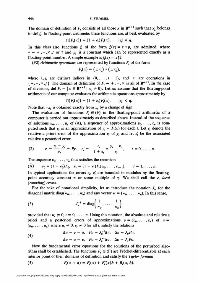
The domain of definition of F, consists of all those x in Rn+1 such that x, belongs
to def/,. In floating-point arithmetic these functions are, at best, evaluated by
fl(F,(*)) = (1 + e,)F,ix), \e,\ < tj.
In this class also functions /, of the form /(z) = z ° p, are admitted, where
° = + , — ,x,l or f and p, is a constant which can be represented exactly as a
floating-point number. A simple example is/,(z) = z\2.
(F2) Arithmetic operations are represented by functions F, of the form
F,(*)-(±^)°(±*t),
where i„j, are distinct indices in {0, . . . , t — I), and ° are operations in
{ + ,-,X,/}. The domain of definition of Ft = + ,-,X is all of Rn+1. In the case
of divisions, def Ft = {x E Rn+1 | x,, ¥= 0). Let us assume that the floating-point
arithmetic of our computer evaluates the arithmetic operations approximately by
ñ(Ft(x)) = (1 + et)F,ix), \e,\ < tj.
Note that -x¡ is obtained exactly from x¡ by a change of sign.
The evaluation of functions Ft E (F) in the floating-point arithmetic of a
computer is carried out approximately as described above. Instead of the sequence
of solutions Uq, .. . ,un of (A), a sequence of approximations t>0, .. ., v„ is com-
puted such that v, is an approximation of y, = F,iv) for each t. Let e, denote the
relative a priori error of the approximation v, of v, and let e't be the associated
relative a posteriori error,
n\ v> ~ y> o, » e< y< ~ v> . n(2) ,, = __=/>„ '<--TTlt-—> t=0,...,n.
The sequence v0, . . . ,vn thus satisfies the recursion
(Â) v0 = (1 + e0)F0, v, = (1 + e,)F,(u„, . . ., v,_x), t = 1, . . . , n.
In typical applications the errors e,, e't are bounded in modulus by the floating-
point accuracy constant tj or some multiple of tj. We shall call the et local
irounding) errors.
For the sake of notational simplicity, let us introduce the notation Jw for the
diagonal matrix diag(w0, . . ., wn) and any vector w = (wq, . . ., wn). In this sense,
(3) •/"' = diagl —,...,—),\w0 wj
provided that wt ¥= 0, t = 0, . . . , n. Using this notation, the absolute and relative a
priori and a posteriori errors of approximations v = (t>0, . . . , v„) of u =
(u0, . . . , u„), where u, ¥= 0, v, ¥= 0 for all t, satisfy the relations
Au = v - u, Pu = J~xAu, Au = JuPu,(4)
Av = u - v, Pv = Jv xAv, Av = JvPv.
Now the fundamental error equations for the solutions of the perturbed algo-
rithm shall be established. The functions Ft E (F) are Fréchet-differentiable at each
interior point of their domains of definition and satisfy the Taylor formula
(5) Fix + h) = F,ix) + Ft'ix)h + Ä,(x, h).
License or copyright restrictions may apply to redistribution; see http://www.ams.org/journal-terms-of-use

EVALUATION ALGORITHMS OF ARITHMETIC EXPRESSIONS 445
The gradients F/(x) of Ft have the form
I dF dF \
because Ft depends on x0, . . . , x,_x only. Input operations Ft E (FO) are constant
functions so that
(7) F¡ix) = 0, R,ix;h) = 0.
For elementary functions F,ix) = fixj) one obtains, from 1.1.(10) with a = x,, a' =
x'j = Xj + hj, the representation
(8) Ft'ix)h = f'iXj)hj, R,ix; h) = /[*,, xp x¡]h2,
where it is assumed that the line segment x,xj belongs to def/. Additions and
subtractions F,(x) = x¡ ± Xj give
(9) Ft'(x)h - h, ± hj, R,ix;h) = 0.
For multiplications F,(x) = x,x, it is seen from 1.1(3) that
(10) F,'ix)h = Xjh, + x,hj, R,ix;h) = h,hj.
In the case of divisions one finally has
(11) Ft'ix)h = -h,..- 4h,, R,ix;h) = -+ F'tix)h,X¡ XT X:
J Aj J
provided that x ^ 0, x'j ̂ 0.
The next theorem constitutes the basis for subsequent error estimates. It shows
that the remainder term of the Taylor formula can be estimated locally uniformly
in suitable neighborhoods of u.
(12) Let the solution u of the algorithm (A) be an interior point of def Ft and ut =£ 0
for all t. Then there exist positive constants k,, £, such that uniformly for all x, h in
(0 <Z, < £„ t = 0, . . . , n,
the joins x, x + h belong to def F't, the components x, do not vanish, and the
remainder terms satisfy the estimates
(Ü) R,(x;h)F,ix)
< Kt[max\PXj\) , t = 0,...,n,j<i
where Pxj = hj/xj.
Proof, (i) As u is an interior point of def F, for all t, there are positive constants
£,° < 2/3 such that all x in the neighborhood \x, — u,|/|u,| < £,°, / = 0, . . ., n, of
u belong to def F[ for all t. Consider first those indices t such that Ft E (Fl), that
is, Ftix) = ftiXj). Then u¡ is an interior point of def/, and there are positive
constants £,x < £,° such that all x, satisfying \xJt — «,;|/|«¿| < Z¡! Del°n8 to def/„
where /, is twice continuously differentiable. Since /,(«,-) = «, ¥= 0, £x may be
chosen so small that also /(x, ) ^= 0 for xy- in this neighborhood. For all indices
k ¥=j, and F, E (Fl) put |¿ = ¿°. Finally let ¿, = |4" for r = 0,.. . , n.
(ii) By virtue of the condition £, < i£,0, t = 0, . . . , n, the line segments x, x + A
belong to def F¡ for all r = 0, . . . , n, whenever x, h is in the neighborhood (12i) of
License or copyright restrictions may apply to redistribution; see http://www.ams.org/journal-terms-of-use

446 F. STUMMEL
u, 0. Since £, < 1, x, ¥= 0 for all t. For input operations, additions and subtractions,
(12ii) holds trivially with k, = 0. In view of (10), the remainder term estimate then
holds for multiplications with k, = 1. In the case of divisions one has
1
F(x)R,ix;h) =
1
1 + PXjÍPX¡ - PXj)PXj, i = i„j =jr
Now £k <2èk < y for all k, and consequently
§«,.1^*1 =
Hence the estimate (12ii) is true for k, = 4. Finally, consider those t such that
F, E (Fl), that is, F,(x) = /,(*)). The estimate (12ii) then follows from (8) and
1.1(11) using the constants
_21
k, = -r maxXJ
l/,(*,)lthe maxima being taken over all Xj, z} such that
max\f,"izj)\,
UJ<%,
uj<Uj, f=Jr D
Applying Taylor's formula to the solutions x = u, x + h = v of the algorithm
(A) and its perturbation (A) gives
(13) F,(o) = F,iu) + F/(m)Au + R,iu; Au),
where h = v — u = Au, and thus
t>, - (1 + e,)(u, + F/(«)A«i + Ä,(u;Au)}.
The absolute a priori errors Au, = v, — u, therefore satisfy the system of equations
(14) Au0 = u0e0, Au, - F,'(u)Au = u,e, + 7;, t = 1, . . . , n,
and the relative a priori errors Put = (u, - u,)/u, the system
(15) />u0 = e0, Pu,-F;iu)JuPu = e, + — T„ t = 1, . . . , n,u, u,
using the remainder terms
(16) T, = e,F/(u)A« + (1 + e,)F,(u;Au).
Similarly, the Taylor formula can be applied for x = v, x + h = u and h = u —
v = Au. Then
F,(«) = F,(c) + F;(o)Ao + /?,(«; Ac).
From (A), (A), and (2) it is seen that F,iu) = u, and
F(t>) = (l + e>„ 1- T- < =v, F,iv) v,' "' 1 + e,-
Hence the absolute a posteriori errors Av, = u, — v, satisfy the equations
(17) Av0=v0e'0, Av, - F,'iv)Av = v,e¡ + R,iv;Av), t = 1, . . . , n.
By (2), e,' denotes the relative a posteriori error of the approximation v, of F,{v).
Dividing both sides of (17) by v, yields the equations
(18) Pv0 = e'0, Pv,-F;iv)JvPv = e't + - R,iv; Av), t = 1, . . . , n,
License or copyright restrictions may apply to redistribution; see http://www.ams.org/journal-terms-of-use
EVALUATION ALGORITHMS OF ARITHMETIC EXPRESSIONS 447
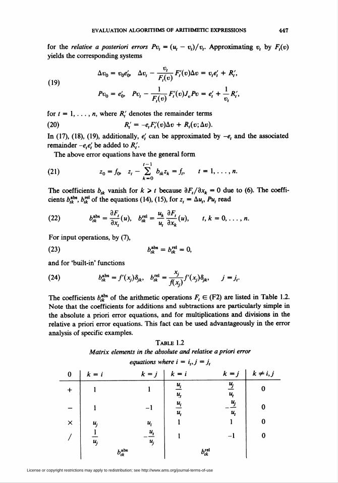
for the relative a posteriori errors Pv, = (u, — v,)/vr Approximating v, by F,(u)
yields the corresponding systems
(19)
AvQ = v0e'0, Av, - -j-F;iv)Av - v,e', + R,',*AV)
Pv0 = e'0, Pv, - -~^ F,'iv)JvPv = e¡ + i R,',
for t = 1, . . . , n, where R,' denotes the remainder terms
(20) R,'=-e,F,'iv)Av +R,iv;Av).
In (17), (18), (19), additionally, e¡ can be approximated by -e, and the associated
remainder -e,e', be added to R¡.
The above error equations have the general form
(21)
t-i
z0 = /o> zr — Zi ^rfczfc = //> * = »,*=0
,n.
The coefficients 6,* vanish for k > t because dF,/dxk = 0 due to (6). The coeffi-
cients bf^, bjk of the equations (14), (15), for z, = Au,, Pu, read
(22)dF,
dx.br («), 6,ï' = ^^(«), t,k = 0,...,n.
For input operations, by (7),
(23)
and for 'built-in' functions
(24)
u, dxk
tabs trel _ A
¿4bs = /'(x,)6}„ ¿»^ = jpjfixj)**, J -Jr
The coefficients ¿>,^bs of the arithmetic operations F, E (F2) are listed in Table 1.2.
Note that the coefficients for additions and subtractions are particularly simple in
the absolute a priori error equations, and for multiplications and divisions in the
relative a priori error equations. This fact can be used advantageously in the error
analysis of specific examples.
Table 1.2
Matrix elements in the absolute and relative a priori error
equations where i = i„j = /,
0 k = i
1
1
k=j k = i k=j
UJ
uj
x
/
uj
uj
k ¥= i,j
0
0
0
0UJ
bttrel°tk
License or copyright restrictions may apply to redistribution; see http://www.ams.org/journal-terms-of-use

448 F. STUMMEL
The representation of the matrix elements in Table 1.2 is so chosen that it also
yields easily computable coefficients of a posteriori error equations. These are
obtained by replacing u,, u,, u, by the solutions v¡, tu, v, of the perturbed algorithm
(Ä). In this way, the absolute a posteriori error equations for additions, subtrac-
tions, and multiplications are given the coefficients
3F(25) ¿-i» = _!(„), k = 0,...,n,
and for divisions F,(u) = vjvj,
(26) «-g«, t** «r-j^ng«.The relative a posteriori error equations for additions and subtractions take on the
form (18), that is, (21) has the coefficients
(27) ¿;ei = ^Íg(ü); fc-0,...,/i,
whereas for multiplications and divisions the form (19) is obtained such that the
coefficients in (21) become
(28) b--wM{v)- *-*••••*
An error estimate for the solutions of these modified a posteriori error equations will
be given in Theorem 2.2(15).
1.3. The Linear Error Equations. Fundamental notions of the perturbation theory
for evaluation algorithms are the associated mappings F and A = / — F in Rn+1
that will be introduced now. The functions F0, . . ., F„, specifying the algorithm
(A), constitute the vector-valued mapping
(1) Fix) = (F0(x), . . . , F„ix))
for all x E Rn+1 such that x E def F, for all t. The solution u = (uq, . . . , u„) of the
algorithm (A) may thus be viewed as fixed point of F,
(2) u = Fiu).
Let v = (u0, . . . , v„) denote the solution of the perturbed algorithm (A). By
inserting v into (2), the associated residual d = v — F(u) is determined. In view of
1.2.(A), obviously,
(3) d, = e,F,iv) = -e',v„ t = 0, . . ., n,
that is, d = -Jce'.
The algorithm (A) defines uniquely the mapping
(4) Ax = x - Fix) = iA0x, . . . , A„x),
having the components
Atyx = *o ~ F), A,x = xt - FÀX)> t = 1, . . . ,n,
for x E def A = def F The solution u of the unperturbed algorithm (A) is, by (2),
a solution of the functional equation
(5) Au = 0,
License or copyright restrictions may apply to redistribution; see http://www.ams.org/journal-terms-of-use

EVALUATION ALGORITHMS OF ARITHMETIC EXPRESSIONS 449
and the solution v of the perturbed algorithm (A) satisfies the equation
(6) Av = d,
using the residual vector (3). In this way, the error analysis of the perturbed
algorithm becomes a perturbation theory of the mapping A in a neighborhood of u.
From Section 1.2 it follows that the mappings F, A are Fréchet-diff erentiable at
each interior point of their domain of definition. The derivative F'(x) of F is
represented by the matrix
(7) n*>-(!r<*))\dXk l,,k-0,...,n
and the associated remainder term by
(8) RFix;h) = F\x + h) - Fix) - F\x)h = (Jtf*;A)),-o...., „,
where R, denotes the remainder terms of the Taylor formula 1.2(5). Hereby also the
mapping A is differentiable at all interior points of def A = def F, where
(9) A'x = / - F\x), x E def F,
and
(10) RAix;h) = Aix + h) - Ax - (A'x)h = -RFix;h).
The derivative A'u is called the derivative of the algorithm (A) and correspondingly
A'v the derivative of the perturbed algorithm (A). From the representation 1.2(6) of
the gradients F/(x) it is seen that the matrix of A'x is lower triangular and its
diagonal elements are equal to 1. Consequently,
(11) A'x is a bijective linear mapping of'R"+1 for each x E def A' = def F'.
Using these mappings, the absolute and relative a priori error equations 1.2(14),
(15) may be written in the concise form
(12) iA'u)Au = Jue + T, iA'u)ieX Pu = e + J~XT.
Analogously, the absolute and relative a posteriori error equations 1.2(17), (18)
read
(13) iA'v)Av = Jve' + R, iA'v)TeX Pv = e' + JVXR,
where
(14) iA'u\eX = J-\A'u)Ju, iA'v)nX = J;\A'v)Jv.
We shall see in Section 2.1 that the remainder terms R, T are of second order in e
as long as the local errors are bounded by \e,\ < e, \e',\ < e, and e is sufficiently
small. Hence neglecting the remainder term T in (12) yields the associated linear a
priori error equations
(15) (A'u)s-Jue, iA'u)nXr = e.
Similarly, by neglecting R in (13), the linear a posteriori error equations
(16) iA'v)s = Jve', iA'v)reX r = e'
are found. We shall prove in Chapter 2 that the solutions s, r of (15) approximate
the a priori errors Au, Pu and the solutions s, r of (16) approximate the a posteriori
errors Av, Pv.
License or copyright restrictions may apply to redistribution; see http://www.ams.org/journal-terms-of-use

450 F. STUMMEL
The eight linear systems (12), (13), (15), (16) have, by (9), (14), the general form
(17) z-Bz=f
using the mappings
B
(18) a priori
a posteriori
absolute
F'iu)
F'iv)
relative
JuF'i»)JU
Jv-lF'iv)Jv
Explicit expressions for elements b,k of the associated matrices of these mappings B
have been listed already in Table 1.2. The solutions z in (12), (13) are given by
(19) a priori
a posteriori
absolute
Au
Av
relative
Pu
Pv
The right-hand sides of the linear error equations (15), (16) read
(20) a priori
a posteriori
absolute
J..e
J„e'
relative
As we have stated above, A'u, A'v and thus iA'u)nX, iA'v)nX are bijective linear
mappings. In order to simplify notation in the further study, the associated inverse
operators are called solution operators and are denoted by L. The solutions of the
above eight linear systems are then written
(21) z = Lf, L = il- B)~x.
In the case of the a priori error equations,
(22) Labs = (il'«)-1, LnX = iA'u)-¿u
and, consequently,
(23)Labs = J..LnXJ. LnX = JjxLahsJ,
Correspondingly, for the associated a posteriori error equations
(24)
whence
(25)
Labs = (A'v)-1, LnX = (A'vYÀi,
Labs = J.,LnXJ, ucl = y,r'Labs/„.
The representation L = (/ — B) ' immediately yields the relations
(26) L = BL + / = LB + I.
Componentwise, the first relation reads
/-i
Ltk = 2 b„L,k + Slk,l-k
k = 0,...,t,(27)
because
(28) bik = 0, i < k, L* = 0, i < k.
A recurrence of this type for computing the entries of the matrix L is found in
Henrici [8, (16-19)]. From the second relation in (26) one obtains
(29) L„ — 1, L,k — ¿j L,¡b¡k,l-k + l
k = 0,. . . ,t - 1.
License or copyright restrictions may apply to redistribution; see http://www.ams.org/journal-terms-of-use

EVALUATION ALGORITHMS OF ARITHMETIC EXPRESSIONS 451
Using the row vectors
Lt = iLtk)k-o,...,»» b, = ib,k)k_0.„, 8, = (S,0, . . . , S,„),
we can write L = LB + / in the form
(30) L, = 2 LA + 8,./=i
Now, put
W- S Lt,b, + S„ 7 = 0,...,/.r«/+t
From (28), (29) it is seen that
L$ = 2 Vfc " L,k> j <k,k = 0,...,t-l,l=k+\
thus, in particular, Ltj = Lfp. Consequently, the row L, of the matrix L can be
computed recurrently from
(31) L<'> = 8„ L</-V = ¡fJ) + L<j)bj, j = t,...,l,
and
(32) L, = Lf\
This is the algorithm (T) of Linnainmaa [10] applied to the computation of the row
L, of the matrix L from the rows of the matrix B. The same algorithm has been
proposed by Larson-Sameh [9] in a somewhat different setting.
2. Condition Numbers, Error Estimates, Graphs. In Sections 2.1, 2.2 it will be
shown that the solutions s, r of the linear a priori and a posteriori error equations
yield approximations of the a priori errors Au, Pu and a posteriori errors Aü, Pv.
Simultaneously, estimates of these errors will be obtained. A fundamental tool of
the error analysis is the notion of condition number. The error approximations s„ r,
are linear forms in the local errors specifying the perturbations of the algorithm.
Our condition numbers are norms of these linear forms with respect to suitably
chosen weighted maximum norms over the space of local errors. Therefore condi-
tion numbers are optimal bounds of the error approximations s,, r, for all local
errors in the considered distribution. Consequently, also the associated estimates of
the errors Au, Pu and Au, Pv are optimal if terms 0,(e) are neglected against 1. In
addition, Section 2.2 demonstrates that the solutions of the linear a posteriori error
equations are approximations of the associated solutions of the a priori error
equations and thus the a posteriori condition numbers approximations of the a
priori condition numbers. Moreover, it will be shown that, using solutions of the
linear a posteriori error equations, approximations of about double precision can
be computed.
Each algorithm and its uniquely associated system of linear error equations
determines a graph, defined in Section 2.3. Graphs constitute useful means of the
error analysis, particularly also for deriving condition numbers of the algorithm.
For example, if the graph is a tree, the condition numbers can be determined a
priori and be computed a posteriori by simple recursion formulae. In all cases,
bounds for condition numbers and hence for error estimates can recursively be
obtained and computed a posteriori. For examples we refer to Stummel [17]—[23].
License or copyright restrictions may apply to redistribution; see http://www.ams.org/journal-terms-of-use

452 F. STUMMEL
2.1. A Priori Condition Numbers and Error Estimates. In the preceding sections
the general linear error equations have been established for the class of algorithms
considered here. Using the associated solution operators L = (/ — B)~x, the solu-
tions z of these linear systems have the form z = Lf. Due to 1.2(6), 1.3(18), the
mappings B are represented by lower-triangular matrices with zeros as diagonal
elements. Consequently, the matrices of the solution operators are lower triangular
with all diagonal elements equal to 1. By Lik are meant the (n + l)2 elements of the
matrix of L. Then
(-1
(1) z, =/, + 2 L,Jk, t = 0,...,n,k-0
as
L„ = 1, L,k = 0, t <k.
For each / the right-hand side of (1) is a linear form L, over Rn+1. Evidently,
(2) L, = pr, L,
where pr, is the projection onto the tin coordinate axis. The solutions s„ r, of the
linear a priori error equations 1.3(15) then have the representation
(3) s, = LabV„e, r, = L,rele.
Of fundamental importance in the following are the associated absolute and
relative a priori condition numbers
(4) a,1 = 2 |l£X|, ft1 = 2 14*1, t = 0,...,n.k=0 k=0
From L„ = 1 it follows that
(5) p¿ = 1, p,1 > 1.
By virtue of 1.3(23),
(6) Labs/„ = JuLnl,
thus
(7) s, = u,r„ oj = |u,|p/.
Using the above condition numbers, the solutions s,, r, satisfy the inequalities
(8) |j,| < 0-,'e, \r,\ < pxe,
for all \ek\ < e, k = 0, . . . , n. These estimates are sharp or optimal because the
bounds o,xe, p,xe are attained for the local error distributions
(9) e^ = e sga(láX), cf-esgnW), k = 0,. . ., n.
By these means we are now in the position to establish error estimates for the
approximations s, r of the a priori errors Au, Pu. By 1.3(12), (15), (22), obviously,
(10) Au, - s, = L,abT, Pu, - r, = L^-'F
whence, using (4),
(11) |Au, — st\ < oj maxU-
\Pu, — r,\ < p,1 maxj«
-U
License or copyright restrictions may apply to redistribution; see http://www.ams.org/journal-terms-of-use
EVALUATION ALGORITHMS OF ARITHMETIC EXPRESSIONS 453
n.
,n.
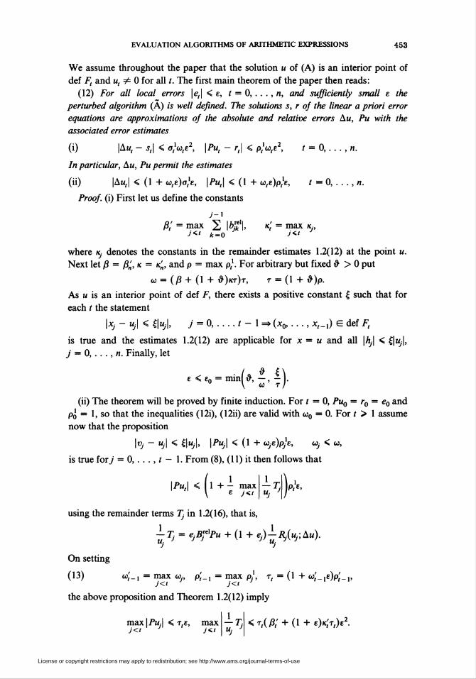
We assume throughout the paper that the solution u of (A) is an interior point of
def F, and u, =£ 0 for all t. The first main theorem of the paper then reads:
(12) For all local errors \e,\ < e, t = 0, . . . , n, and sufficiently small e the
perturbed algorithm (A) is well defined. The solutions s, r of the linear a priori error
equations are approximations of the absolute and relative errors Au, Pu with the
associated error estimates
(i) |Au, - s,| < o-,'co,e2, \Pu, - r,\ < p,'co,e2, / = 0, . .
In particular, Au, Pu permit the estimates
(ii) |Au,| < (1 + w,e)o,xe, \Pu,\ < (1 + u,e)p,xe, t = 0,
Proof (i) First let us define the constants
y-i
2 .J« k=0
where k¡ denotes the constants in the remainder estimates 1.2(12) at the point u.
Next let ß = ß'n, k = k'„, and p = max p,1. For arbitrary but fixed # > 0 put
w = iß + (1 + #)kt)t, T = (l + #)p.
As u is an interior point of def F, there exists a positive constant £ such that for
each t the statement
\xj - Uj\ < %|, j = 0,-t - 1 => (x0, . . ., x,_x) E def F,
is true and the estimates 1.2(12) are applicable for x = u and all |/i,| < £|u,|,
/ — 0,..., n. Finally, let
ft' = max 2 !/#, k, = max k ,/« y
e < £0 = minI ' w' t/'
(ii) The theorem will be proved by finite induction. For / = 0, Pu0 = r0 = e0 and
p¿ = 1, so that the inequalities (12i), (12ii) are valid with w0 = 0. For t > 1 assume
now that the proposition
\vj - Uj\ < i\uj\, IPu,I < (1 + u>je)pxe, w,- < co,
is true for/ = 0, . . . , t — 1. From (8), (11) it then follows that
\Pu,\ < ( 1 + - max — T )pxe,\ « J« "j J J
using the remainder terms Tj in 1.2(16), that is,
-Tj = ejBfPu +il +ej)-RjiUj; Au)
On setting
(13) w;_! = max co,., p',_x = max pj, t, = il + u',_xe)p',_x,
the above proposition and Theorem 1.2(12) imply
max | Pu | < t,£, maxj« j<t Il J
<r,iß; + il + e)K',T,)e2
License or copyright restrictions may apply to redistribution; see http://www.ams.org/journal-terms-of-use

454 F. STUMMEL
Consequently,
1 2< Í0,£: ,max
j<t-Tju Jj
where co, = t,(/3,' + (1 + e)k',t,), t = I, . . . , n. Finally, the above proposition en-
tails co,'_i < to, t, < (1 + coe)p < t. Thus to, < ( ß + (1 + #)kt)t = to and
= |Pu,| < (1 + u,e)p}e < te < £
for all e < £0. Hence the above proposition is true also for/ = t and consequently
for all / = 0, . . . , n. The estimates of the remainder terms TJu„ proved above,
immediately yield the error estimates (12i), (12ii). □
The above theorem guarantees that the solutions s, r of the linear error equations
are equal to the a priori errors Au, Pu save for terms of second order in £,
(14) Au, = s, + 0,ie2), Pu, = r, + 0,(e2).
On this basis, error estimates can be derived regarding specific distributions of the
local errors. Let us assume that
(15) \e,\ < y,?), t = 0, . . .,n,
where y0, ■ ■ ■ , y„ are appropriate nonnegative weights. Theorem (12) applies to this
specific distribution of local errors in choosing e = max y,Tj. However, the solutions
of the linear error equations can be estimated finer by
(16) \s,\ = \L?sjue\ < a,Tj, |r,| = |L,rele| < p,Tj,
using the weighted absolute and relative a priori condition numbers
(17) a, = 2 l¿AlY*, P, = 2 1^'lY*, / = 0,. . . , n.k=0 k=0
In cases, for example, when F, is an input operation of a floating-point number
represented exactly in the computer, the associated y, may be set equal to zero.
When a subtraction F, is performed with loss of significant figures but without
rounding error, we may put y, =0. If a built-in function F, = /, is evaluated in
lower precision than the arithmetic operations are, the associated y, may be chosen
suitably greater than 1. In particular, the behavior of the algorithm under data
perturbations only and under rounding errors in the 'built-in' functions and
arithmetic operations only can be analyzed. For this purpose, to a given sequence
of weights (y,) of the local error distribution, put
(18i) Y,° = y„ F, E(F0); y,R = y„ F, £ (Fl) U (F2);
and y,D, y,R = 0 else for / = 0, . . . , n. The sequences of weights {y,D), (y,Ä) specify,
by (17), weighted absolute and relative data condition numbers of, p,D and rounding
condition numbers o,R, p,R. In this way, the decompositions
(18ii) Y.-Y^ + Y,* o, = a,D + a,R, ft - pf> + p*
are obtained. The following corollary states error estimates using weighted condi-
tion numbers.
(19) Let any nontrivial sequence of weights y0, . . . , yn be given. For every sequence
of local errors in the distribution (15) and sufficiently small e = yrj the solutions of the
License or copyright restrictions may apply to redistribution; see http://www.ams.org/journal-terms-of-use
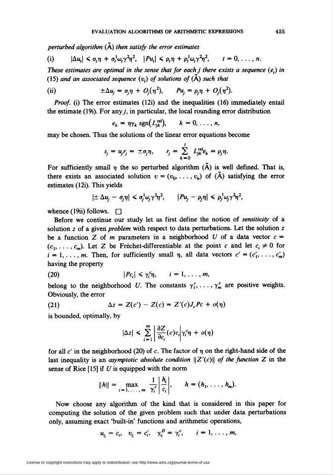
EVALUATION ALGORITHMS OF ARITHMETIC EXPRESSIONS 455
perturbed algorithm (A) then satisfy the error estimates
(i) |Au,| < o,Tj + o,xio,y\2, \Pu,\ < p,Tj + p/to^V, t = 0, . . . , n.
These estimates are optimal in the sense that for eachj there exists a sequence (t?,) in
(15) and an associated sequence (u,) of solutions of (A) such that
(ii) ±Auy = Oj-q + Ojin2), Puj = fti, + 0,(tj2).
Proof, if) The error estimates (12i) and the inequalities (16) immediately entail
the estimate (19i). For any/, in particular, the local rounding error distribution
«* - vrtk sefl(LJk)> k=0,...,n,
may be chosen. Thus the solutions of the linear error equations become
t
Sj = UjTj = ±OjH, Tj = 2 Lßfck = PjV-k-0
For sufficiently small tj the so perturbed algorithm (A) is well defined. That is,
there exists an associated solution u = (u0,.. . ,vn) of (A) satisfying the error
estimates (12i). This yields
|± Au,. - o,tj| < cr/to^Y, \Puj - p,Tj| < p^yV.
whence (19ii) follows. □
Before we continue our study let us first define the notion of sensitivity of a
solution z of a given problem with respect to data perturbations. Let the solution z
be a function Z of m parameters in a neighborhood ¿7 of a data vector c =
(c„ . . . , cm). Let Z be Frechet-differentiable at the point c and let c, =£ 0 for
i = 1, . . . , m. Then, for sufficiently small tj, all data vectors c' = (c\, . . . , c'm)
having the property
(20) |Fc,| < y,% i = l,...,m,
belong to the neighborhood U. The constants Y*» • ■ • » Y« are positive weights.
Obviously, the error
(21) Az = Zic') - Zic) = Z\c)JcPc + o(tj)
is bounded, optimally, by
3Z.|Az| < 2
6V(C)C'y,cTj + o(tj)
for all c' in the neighborhood (20) of c. The factor of tj on the right-hand side of the
last inequality is an asymptotic absolute condition ||Z'(c)|| of the function Z in the
sense of Rice [15] if U is equipped with the norm
c,\\h\\ = max —
(-1, ...,m y,h = (A„ . . . , hj.
Now choose any algorithm of the kind that is considered in this paper for
computing the solution of the given problem such that under data perturbations
only, assuming exact 'built-in' functions and arithmetic operations,
u, = c„ u, = c'¡, y,f = y,c, /'=!,..., m,
License or copyright restrictions may apply to redistribution; see http://www.ams.org/journal-terms-of-use

456 F. STUMMEL
y,D = 0 f or / £ {/,, . . . , tm), and Zic) = u,, Zic') = v, for all c' in the neighbor-
hood (20) of c. Thus, on the one hand (21) holds and on the other hand, by (3),
(14),
Au, = L,absV° + 0,(tj2),
where e,D = Pc¡, e,D = 0 for t £ {r„ . . ., tm). Consequently,
L^JueD = Z'ic)JcPc + o(tj)
for all Pc, = e,D in (20). From this relation one readily concludes that the coeffi-
cients of the two linear forms coincide and, consequently,
(22) of = 2 \V>k\ykD = 2k = 0 i=l
azTcSc)c>y;
This result shows that the value of o,D is independent of the special evaluation
algorithm and a measure of the data sensitivity of the solution of the given
problem.
The well-known backward analysis represents perturbations of the algorithm
under rounding errors by means of data perturbations. This procedure may now be
specified quantitatively as follows. Error distributions (15) with the weights (y,Ä)
and accuracy constant tj = t\R induce perturbations of function evaluations and
arithmetic operations only, the data remain unperturbed. By Theorem (12) and
(16), (17), the absolute errors (Am,)* = v,R — u, of the sequence (u,*) of solutions of
the so perturbed algorithm satisfy the relations
(Au,)* = s,R + 0,(V2), \s,R\ < a,V
For any index/ such that of ¥^ 0 choose the data accuracy
„R „*j Pj
(23) tjd = —-r¡R =—¿t]R.Oj Pj
Under data perturbations only, the associated linear forms Lf*JueD then have the
closed intervals
[-0-/V +ofvD] =[-o,%, +ay%]
as their range. Hence, sf belongs to this range and there exists a sequence eD of
local errors in \e,D\ < y,Dr¡D such that sR = Lf°&JueD = sf. By virtue of Theorem
(12), using this sequence eD of local errors and the accuracy constant r\D, there
exists a sequence (u,D) of solutions of the algorithm under data perturbations only
such that (Au,)° = s,D + G,(tj¿). It follows from the above that t)0 is the least
constant such that the absolute error (Au,)fl = vf — u} gives the representation
(Am,-)* = (Am,-)d + Ojir\R) for arbitrary local rounding errors e,R in \eR\ < y/^rj*.
Consequently, the constant oR/'of = pf/pf measures the stability of the algo-
rithm for computing m, in the sense of Wilkinson's backward error analysis [25,
1-39].
An algorithm is called by Bauer [4], [5] well-conditioned (German: gutartig) if the
influence of rounding errors in the arithmetic operations is at most of the same
order of magnitude as the influence of data perturbations whose magnitude
License or copyright restrictions may apply to redistribution; see http://www.ams.org/journal-terms-of-use

EVALUATION ALGORITHMS OF ARITHMETIC EXPRESSIONS 457
corresponds to rounding errors. Thus the computation of u, by the algorithm (A) is
well-conditioned if the estimates
(24) a* < ßof, p,R < ßpf
hold where the constant ß is not much greater than 1.
Example 1. The product algorithm
(25) "o=*o, ut = b,u,_x, t=l,...,n,
for the computation of un = II"=0 b, possesses the condition numbers
(26) p,D = t + 1, p,R = t.
Hence p,R < p,D, so that this algorithm is well-conditioned. □
Example 2. The summation algorithm
(27) u0=c0, m, = m,_, + c„ t = 1, . . . , n,
for the computation of the sequence of partial sums u, = 2'^_0 ck, t = 0, . . ., n,
has the condition numbers
(28) o-,° = 2 14 o-* = 2 14y-0 7=1
In the case of nonnegative terms it follows that
(29) p,D=l, PR = ^íuj<t.utj=\
Consequently, the summation algorithm for the computation of un is well-
conditioned if and only if pR is not much greater than 1, so that the relative error
Pun is bounded by a low multiple of the floating-point accuracy constant tj. This
condition is not true in many cases. A well-known concrete example is the
summation of c, = « for/ = 0, . . ., n. In this case
(30) u, = it+l)h, P,R=J^\-{> t=l,...,n.
For
h = .555, « = 200, m„ = 111.555, pR = 101,
in 3-digit decimal floating point u„ = 133, Pu„ = .192, is computed. Here tj =
5.-03, p,frj = .505, so that this bound overestimates the error only by a factor of
2.63. D2.2. A Posteriori Condition Numbers and Error Estimates. In many examples the
condition numbers of the algorithm or appropriate bounds can be computed from
the data and intermediate results arising during the computation. For this purpose
the a posteriori condition numbers are needed, being specified by the sequence of
solutions v0, . . . ,v„ of the perturbed algorithm (A). The linear a posteriori error
equations 1.3(16) yield, together with the solution operators 1.3(24), the approxima-
tions
(1) s, = L^Je', r, = Ufe',
License or copyright restrictions may apply to redistribution; see http://www.ams.org/journal-terms-of-use

458 F. STUMMEL
of the a posteriori errors Au,, Pv,. The associated weighted a posteriori condition
numbers
(2) 2 \L$\\yk, p, = 2 \L]k\ykk=0 fc-0
are optimal bounds in the estimates
(3) |s,| < a,Tj', |r,| < p,Tj'
for all local relative a posteriori errors \e'k\ < y^Tj', k = 0, ...,«. In view of 1.3(25),
(4) s, = v,r„ o, = |o,|ft.
The aim of the following investigation is to compare the solutions of the linear a
priori and a posteriori error equations as well as the a priori and a posteriori
condition numbers. For distinctness the upper index i indicates a priori terms from
Section 2.1 and the upper index 0 a posteriori terms defined above. In addition, the
nonweighted a priori condition numbers
(5) *»' - 2 \LÍk«kl P/=TTT> ' = 0, ,",k = 0
are used in error estimates, V denoting the absolute a priori solution operator
(A'u)-1.
The first lemma is basic for the following. It shows that the derivatives F',A' =
I — F' are Lipschitz continuous at u.
(6) There exist constants f, such that for all local errors \ek\ < e, k ■» 0,..., n, and
sufficiently small e the following inequalities are valid:
(i)
t-\
2* = 0
uk(dF dF, \<?, rnax\Puk\,
k<tt =0,
Proof, if) For those t for which F, is an input operation, dF,/dxk = 0, so that the
above inequality holds trivially with f, = 0. For additions and subtractions F„ the
partial derivatives dF,/dxk are constant and equal to 0, +1, -1 for each k. Hence
for these / the left side in (6i) vanishes, and the inequality is true too with f, = 0.
(ii) Next consider the indices t such that F, is a multiplication. As is readily seen,
now
r-i
2* = 0
dF, dF,
u, \dxk 3x,= \I\\ + \Pu,
whence (6i) follows using the constant f, = 2.
(iii) By virtue of Theorem 2.1(12), there exists an e, such that for all e < e, the
solutions u, of the perturbed algorithm (A) are in the neighborhoods defined by
1.2(121). In particular, then |Pu,| < j for all t. One easily verifies the estimate
k = 0
U« (dF'í \ dF> ( \\ 2\Puj\ \Puj - Pu¡\
|1 + Puj\ \l+PUj\
for divisions F,(x) = xi/x,. As |Pu,| <\, the denominators are bounded from
below by \ and \. Thus the inequality (61) holds in this case with f, = 7.5.
License or copyright restrictions may apply to redistribution; see http://www.ams.org/journal-terms-of-use

EVALUATION ALGORITHMS OF ARITHMETIC EXPRESSIONS 459
(iv) In function evaluations F,(x) = /,(*,), i = /'„ finally,
k = 0
"k / 9F , s 3F,— -5— iv) ~ ~5-~iuu, \ dxk dxk
u2
/,(»,)rr/ZV,)/5",
vw(- being some intermediate point of the line segment u¡v¡. By Theorem 1.2(12), the
join uv belongs to the domain of definition of F'. The right-hand side of the last
equation is bounded by 2k,|Pm,|, using the constants k, of Theorem 1.2(12).
Consequently, (6i) is true for f, = 2k,. □
By the above lemma, we can now estimate the distance between the a priori and
a posteriori solution operators
(7) V = (A'u)-\ L° = iA'v)-1.
(8) There exists a constant p such that for all local errors \ek\ < e, k = 0, . . . , n,
and sufficiently small e the associated solution operators suffice the following estimates
t
(O 2 14° - ¿ilkl <°,V. t = 0,...,n.k=o
Proof, (i) As is readily verified, the difference of the solution operators has the
representation
l° - v = -//(/+ cyxc,
where C = iA'v - A'u)V = (F(") - F'iv))V. This implies
(9) (L° - V)JU = -L'JM + D)lD,
using the notation
D = jfCJu = JfiF'iu) - F'iv))VJu.
Let us further denote by Ja the diagonal matrix diag(a¿, . . . , an'). In the maximum
absolute row sum norm then
(10) WJfL'JJ = max -1 ¿ \L¡kuk\ = 1.' o, k = o
The matrix D is bounded in this norm by
«*/3F, 3F \|fl|| < ||/-»(F'(«) - F'(ü))yj| = max 2
' A;=0a|.
From Lemma (6) we infer the further estimate
(11) \\D\\ < fp max|Pu,|, f = max f„ p = max p,1.« r »
Now choose any constant & in 0 < & < 1 and put
/ & tr \t = (1 + #)p, e < minlE,, —, -r— I,
Theorem 2.1(12) then guarantees that
max|PM,| < (1 + (¿e)pe < te.
License or copyright restrictions may apply to redistribution; see http://www.ams.org/journal-terms-of-use

460 F. STUMMEL
The above estimate (11) hereby yields \\D\\ < fpre < d < 1. Finally (9), (10), (11)
entail the estimate
\D\\\JfiL0 - L'yjl < < I*,
\-\\D\
using the constant fi = fpr/(l — #), and thence the asserted inequality (8i). □
Having made these preparations, we are in the position to prove the comparison
theorem. By s', r' are meant the solutions of the linear a priori error equations
1.3(15), and by s°, r° the solutions of the linear a posteriori error equations 1.3(16).
Further, a,', p,' denote the weighted a priori condition numbers 2.1(17) and a,0, p°
the a posteriori condition numbers (2).
(12) For all local errors \ek\ < yki), k = 0, . . . , n, and sufficiently small tj the
approximations of the absolute and relative a priori and a posteriori errors satisfy the
relations
0) ,o = _s/ + 0,(t,2), r° = -r¡ + 0,(tj2),
and the associated weighted condition numbers the relations
(ii) a,0 = a,' + <9,(tj), p,° = p/ + 0,(tj).
Proof, (i) The solutions of the linear absolute a priori and a posteriori error
equations have the representations s' = L'Jue, s° = L°Jve'. Thus,
s,' + s? = Ll(Ju - Jv)e + L',Jvie + <?') + (L,° - L¡)Jve'.
The first term on the right side is bounded by
\L,Vu - JM < 2 \L,kukPukek\ < a/||Pu||Tj,*=o
using the maximum norm for Pu. By virtue of 1.1(8), ek + e'k = -eke'k. For
\ek\ < ykt) it follows that
141- 1 + e.
ykV
i<
mYTJ, maxy*, y =
1 - Y"
Therefore, the second term on the right side suffices
\LJJv(e + e')\ < 2k=0
L>k—eke'kuk
<0,'(l + ||Pu||)y'T,2.
By virtue of Lemma (8) for e = yrj, the third term can finally be estimated by
|(I° - L¡)Jve'\ < 2*=o
o*(Ll-L¡k)uk^-e' < a,'uy(l + ||Pw||)y'T,2
On choosing e as small as in the proof of Lemma (8), we have \\Pu\\ < re and
||Pm|| < j. The above appraisals then entail |j/ + s,°| < (0,'<j> + o,V)tj2, using the
constants
<#> = Ty + j y', «i'=3/XYY'.
(ii) The solutions r', r° of the linear relative a priori and a posteriori error
equations permit the representation
1 Í s,' + sf0 _r' + r =i, -r i,
1 + Pu,+ r\Pu,
License or copyright restrictions may apply to redistribution; see http://www.ams.org/journal-terms-of-use

EVALUATION ALGORITHMS OF ARITHMETIC EXPRESSIONS 461
For yrj = e < e,, again |Pu,| < re and \Pu,\ < j. Using the above estimates for
s,' + s,° and 2.1(16), thus
l\r¡ + r?\ < (pi* + p,xt)V2 + p¡Tm2.
(iii) The weighted absolute condition numbers satisfy the relations
|k/-°,°l< t \L;kuk - L^vk\y k=o
< 2 \L;kukPuk\ + 2 |(i£ - L'tk)vk\.k=0 k=0
The first term on the right side can be estimated by
2 \L,'kukPuk\ < al\\Pu\\ < otryt,.k=0
Using Lemma (8), the second term possesses the upper bound
2 |(U - UkO + Puk)\ < 0X1 + || ah).k=0
Hence, for e = yrj < e„ the above yields
I»/ - 0,°| < o,xxn, x = (t + 5/i)y.
(iv) Finally, the difference of the weighted relative a priori and a posteriori
condition numbers is bounded by
i Í w - «,°i
Together with the estimate for |o,' - 0,°| this entails
fk'-ftl < pirn + plvm- DIn computing a posteriori condition numbers or solutions of linear a posteriori
error equations, Table 1.2 yields modified coefficients. The modified relative a
posteriori error equations f — Br = e' for approximations f of Pv are defined by
matrix elements b,k of 5 of the form 1.2(27), (28),
(13) F = +,-: i.-|^(.); *.-X./: 4=^|^),
whereas the elements 6,Ä of the unmodified relative a posteriori error equations
r - Br = e', by 1.3(18), read
We limit the further study to the four arithmetic operations +, -, x, / and
establish the theorem
(15) 77ie approximations r„ r, of the relative a posteriori errors Pv, satisfy, for
sufficiently small e = yrj, the relations
(0 r,= r,+ 0,(tj2),
and the associated weighted relative a posteriori condition numbers the relations
(ii) ft - (1 + 0,ir,))p„ / = !,...,«.
License or copyright restrictions may apply to redistribution; see http://www.ams.org/journal-terms-of-use
462 F. STUMMEL
Proof, (i) The two equations for r, r immediately imply the representation
f -r = LAB?, L = iA'vfrli, AB = B -B.
When Fk = + , —, Abkl — 0, whereas for Fk = X , / we obtain
^hi " b\, - bkl = -e'kbkl
because Fkiv)/vk = I + e'k. The above leads to the estimate
\r, - r,\ < tj' 2 m?\yk 2 IVVI < 2T,'p/max|ry.|k=0 1=0 J<'
Fk=X,/
because \bu\ = 1 exactly twice and zero else for Fk = X , /. Further, the last
inequality yields
maxlr.l < p'rj' + 2Tj'p,'max|//|,7« Jo
using the constants p,' = max,^, p,, tj' = tj/(1 - yrj). Hence
, , °-'max r. <— .VI - 1-2^'
as far as 2p,'Tj' < 1. Inserting this expression into the above inequality for r, — r,,
we obtain
IS rl < 2P'P< W2
and thus the assertion (15i) is proved,
(ii) Next, using appropriate constants \p„
\F,\ < kl + Pf^TJ2, \r,\ < \r,\ + p,\p,n2.
The associated weighted relative a posteriori condition numbers p„ p„ permit the
estimate \r,\ < p,r¡', \r,\ < p,Tj', for all local errors \ek\ < y^rj where y = max yk and
tj' as above. By means of the local errors
h = -Y*1 sgn(L,^), ek = -y^T, sgn(L]f),
we finally conclude
P< <- P> L I P< <- P' L I
1 + yrj 1 - yrj1 + yrj 1 — yrj
hereby proving (15ii). □
By Theorems (12) and (15), we have established the a posteriori error representa-
tion
(16) »,~r, + 0,(tj2),
where r is the solution of the modified linear relative a posteriori error equations.
Solving this relation for u, yields
u, - o,(l + r, + G,(tj2)).
Hence
(17) u,' = o,(l + r,)
License or copyright restrictions may apply to redistribution; see http://www.ams.org/journal-terms-of-use

EVALUATION ALGORITHMS OF ARITHMETIC EXPRESSIONS 463
is an approximation of u, having the relative error (u, — v',)/v', = 0,(tj2). Conse-
quently, v', approximates u, within about double precision. The sequence of
solutions m0, .. ., un of the algorithm (A) may thus be computed in about double
precision from the approximations u, and the solutions r, of the modified linear a
posteriori error equations, both computed in single precision. We call this proce-
dure extrapolation to double precision. The a posteriori coefficients b,k are readily
computed from the data and intermediate results in performing the algorithm. If
the local errors e, are available numerically, the solutions r, of the linear a
posteriori error equations and the extrapolated approximations v¡ can be computed
together with u,.
Table 2.2
Extrapolation to double precision in Cramer's rule
t u, v, e, -f, X103
0 a 0.455 1.00-03 1.00
1 b 0.111 -1.00-03 -1.00
2 c 0.273 1.00-03 1.00
3 d 0.778 2.86-04 0.29
4 / 0.404 -1.00-04 -0.105 g 0.566 6.07-04 0.61
6 ad 0.354 2.82-05 1.317 be 0.0303 -9.90-05 -0.10
8 df 0.314 -9.93-04 -0.819 bg 0.0628 -4.14-04 -0.81
10 ag 0.258 1.83-03 3.44
11 cf 0.110 -2.65-03 -1.7512 D0 0.324 9.27-04 2.36
13 £>, 0.251 -7.96-04 -1.60
14 D2 0.148 0 7.29
15 x 0.775 3.98-04 -3.56 * ~ * = 3.57-03,x
16 v 0.457 4.59-04 5.39 Zl^Z = 540_03v
x = 0.7 ..., x' = 0.775, x" m 0.777 769, *" ~ * = -1.13-05,x
v = 0.45 . . . , y' - 0.457, y" = 0.454 550, y" ~y = 1.00-05.
Example. Two linear equations in two unknowns,
(18) ax + by = /, ex + dy = g,
have, by Cramer's rule, the solution
D\ D2x=n' y=n> (A)*0),u0 u0
License or copyright restrictions may apply to redistribution; see http://www.ams.org/journal-terms-of-use

464 F. STUMMEL
using the determinants
A> =
Consider the numerical example
5 1(19)
P>i =
40
Z>2 =
llJC + 9>, = 99'
3_ 7 5611 ^ 99'
having the solution x = 7/9, v = 5/11. Table 2.2 lists the approximations v, in
solving Cramer's rule using 3-digit decimal floating-point arithmetic, the associated
local rounding errors e, of input and arithmetic operations, and the approximations
r, of the relative a posteriori errors described above. The numerical results show
that the extrapolated results x", y" approximate x, y essentially within double
precision.
2.3. Associated Graphs. In typical applications of the perturbation theory, the
number n of steps and thus of equations in the systems 1.3(15), (16), (17) often
becomes very large. However, the matrices ib,k) of the linear error equations are
sparse; for input operations, F, is constant and b,k = 0 for all k; 'built-in' functions
F, give b,k = 0 for all k ¥^j,; for arithmetic operations F, E (F2), b,k = 0 for all
k ¥= i„j,. Hence the linear error equations have the form of inhomogeneous linear
recursions of zeroth, first and second order with variable coefficients. In general,
however, these equations have a complex structure because z, is not obtained from
z,_x, z,_2 but from z,, z,. This structure can be illustrated by the associated graph
(see McCracken-Dorn [11], Bauer [5]): each t is assigned a point in R2, called node,
and nodes k are connected to the node t by means of a path kt if the coefficient or
weight b,k, that is, dF,iu)/dxk or dF,iv)/dxk can be nonzero. In addition, every path
kt is labelled by its associated weight b,k. By convention, labels 1 may be omitted.
By these means linear error equations can simply be read from the graph of the
algorithm. Figure 2.3 shows the building blocks of the graphs.
The graphs in Figure 2.3 may as well be viewed as graphs of the simplest
numerical algorithms analyzed in Section 1.1. For instance, let
(1) m0 = a, ux = b, m2 = m, ° m0,
using an arithmetic operation ° E{+, -, X, /}. In floating-point arithmetic, this
algorithm is realized by
(2) u0 = fl(a), u, = fl(6), u2 = fl(u, » u0).
The associated linear absolute and relative a priori and a posteriori error equations
and their graphs then have the form shown in Figure 2.3, where / = 0,/ = 1, t = 2,
and r0 = e0 = Pa, rx = ex = Pb.
Graphs constitute important means in the study of solutions of linear systems
(3) Bz =f<=>z, - 2 b,kzk =f„ t = 0, . . . n,k = 0
with sparse matrices, as we will explain now. The matrix B is lower triangular and
its diagonal elements are zero. Thus B is nilpotent and Bn+X = 0. The solutions z
of the linear system may then be represented by the finite Neumann series
(4) z = (/-Jf?ri/=2 B'f-1 = 0
License or copyright restrictions may apply to redistribution; see http://www.ams.org/journal-terms-of-use

EVALUATION ALGORITHMS OF ARITHMETIC EXPRESSIONS 465
i ■© -j -0
u.i
f'(u.)
u - f(u.) f
0-rr^r f'(u.)f(u.) i
0s. = u.e., s. = u.e.
i i i J J J
r. = e., r. - e.i i J J
st = f'(u.)s. -utet
u.
r = ^7^-x f'(u.)r + et f(u.) ii t
s =s.+s.+uet i J t t
u. u.i i
r = — r. + —*• r. + et u i ut j t
s » s. - s. + u et i J t t
u. u.
r = — r. - -J- r. + et ut i ufc j t
s » u.s. + u.s. + u et J i i J t r
r = r. + r. + et i .1 t
V®
ut - u./u.V 0
1st = TT7 si * uT sj + utet
j J
r = r. - r. + et i j t
Figure 2.3
Building blocks of the graphs of linear absolute is,, weights bfl? left of the
path) and relative (r„ weights b]k right of the path) a priori error equations.
The associated a posteriori error equations are obtained by replacing
up Uj, u„ e, by u„ u,., u„ e',.
License or copyright restrictions may apply to redistribution; see http://www.ams.org/journal-terms-of-use
466 F. STUMMEL
The powers of B have the elements
/?° = (¿y, Bx = ibik),
(5) b> = m, bip = 2 • •k, = 0
2 bik*,=o
^2*, t, A: = 0,. . . , n,
for / = 2, . . ., n. As ¿>,fc = 0 for i < k, matrix elements b$ can be different from
zero only if the condition
(6) i > k, > k,_x > ■ ■ ■ > k2 > kx > 0
holds, and therefore
(7) b\£ = 0 for i < k + I
and all / = 1, 2,... . Correspondingly, the components z, of the solution vector z
of (3) possess the representation
(8) z, = LJ = f,+ 2 2 b%% t = 0,...,n.1=1 k=0
In this way, explicit representations of the components L, of the solution operator
L have been obtained. Interchanging the order of summation gives
(9) ,/ = /<,, lj= 2 W*-/«+ 2(2 »ípU,A: = 0 fc=0\/-l /
f « 1, .... B.
Consequently, the matrix elements of the solution operators L = (/ — B) x have
the representation
(10)*•-!. A*" 2 MP, A: = 0-, r - 1 ;
/-iL,* = 0, fc - t + 1.n.
The basis of our further investigations is the explicit representation
/-i í-i ,-i
(H)
z, = LJ = f,+ 2 b,kifk¡+ 2 2 b,kbk]k¡fki +*,=0 k2-0 k,=0
t-l
+ 2*,-0
Í-1
2 btk¡*,=o
bkjctfkl,
ensuing immediately from (5), (8). A sequence of paths kxk2, .. . , k,t of the graph
is a path of length I from the node kx to the node t. We call the associated product
btk, ' ' ' bkikl the error effect and the term b,k¡ • • • bk]k¡fki the error contribution
along this path at the node t. The error effect is simply the product of all weights
along the path. On the right side of (11), evidently, only those terms of the sum can
be nonzero which belong to a path of the graph, all other terms vanish. In view of
(6), necessarily t > k, > - ■ ■ > k2 > kx for every path in the graph. The /-fold sum
in (11) is the sum of the error contributions at the node r along all paths of length /.
The node t itself is assigned the path or loop of length zero and the error effect 1.
The representation (11) may thus be read as follows
(12) The solution z, = LJ of the linear error equations is the sum of the error
contributions along all paths in the graph ending at the node t.
License or copyright restrictions may apply to redistribution; see http://www.ams.org/journal-terms-of-use

EVALUATION ALGORITHMS OF ARITHMETIC EXPRESSIONS 467
On setting especially
/*> = i80k, ...,«*), k = 0,...,n,
as inhomogeneous terms, the associated solutions z, — LJ*® become the matrix
elements L,k of the solution operators L = (/ - B)~x. In particular,
(13) L,k = 2 b$ = b,k+ 2 b,kbk2k +i=i
t-i
2k, = 0
/-I
+ 2k,=0
2 btkifc2-0
"k,k
is the total error effect associated to all paths from the node k to the node t (see
Bauer [5, p. 88]).
Now let us consider our condition numbers in this context. The weighted
absolute and relative a priori and a posteriori condition numbers 2.1(17), 2.2(2)
have the general form
(14)
where
(15)
k=0
a priori
a posteriori
absolute relative
a priori
P, a posteriori
absolute
klY*
I»*|Y*
relative
Y*
Y*
and L,k denotes the matrix elements of the associated solution operators 1.3(22),
(24). The condition numbers are thus weighted sums of the absolute values of the
total error effects. It is readily seen from (14) that
(16) A, = max \Lj\, t = 0,...,n.max | V|,\fk\ <«*
k = 0.n
The maximum is attained forfk = ak sgn L,k, k = 0, . . . , n.
The condition numbers can be computed easily if, for instance, all matrix
elements L,k are nonnegative. This is the case, in particular, if the elements b,k are
nonnegative. Then / — B is a so-called A/-matrix. Under the assumption L,k > 0,
(17) \ = 2 Ltkak = L,a> t =0, . . .,n,k = 0
where a = (oq, . . . , a„). That is, the vector X = (A,,, . . . , \,) of condition numbers
is a solution of the linear system X — BX = a and, consequently, can be obtained
recursively from
t-i
(18) Xq = a0, A, = 2 b,kXk + a„ t = 1, . . ., n.k=0
In the general case, where the weights b,k have arbitrary signs, at least bounds
can be determined for the solutions z, = LJ and thus for the corresponding
condition numbers A,. The above results immediately yield the theorem:
(19) 77te recursion
t-\
(i) H = «o, P» = 2 \btk\Pk + a„k=0
t = 1, . .., n,
License or copyright restrictions may apply to redistribution; see http://www.ams.org/journal-terms-of-use

468 F. STUMMEL
generates a sequence in,) of bounds having the property
(ii) kl = 14/1 < «,» \ < p»,for allf = (/0, ...,/„) such that \fk\ < ak, k = 0, . . ., n.
When an algorithm is built up of input operations and additions only, the
coefficients b,k of the hnear absolute error equations consist, according to Table
1.2, of zeros and ones, that is, B is a binary matrix. The same is true for the hnear
relative error equations when the algorithm consists of input operations and
multiplications only. For a binary matrix B, one readily sees from (13) that
(20) L,k = Number of paths from k to /.
The explicit representations of solution operators and associated condition
numbers become very simple when the graph of the algorithm is a tree. In these
graphs there exists to each k < t exactly one path kxk2, ..., kst from k = kx to t,
where the length s of the path depends on the pair k, t. Now the total error effects
are simply
(21) L„ = 1, L,k = 2 6g> = b,K- ■ ■ bkJc,i=\
and the associated condition numbers have the form
t-i
(22) Xo = ao, X, = 2 1**1 ■ ■ • \bk2k\<*k + «rk=0
In this case, the sequence (X,) is the solution of the recursion formulae
r-1
(23) Xo = a0, X, = 2 \blk\h + «*> ' - 1.«•k=0
For, this system has the form of the linear error equations with coefficients \blk\
and inhomogeneous terms a, instead of b,k,fr According to (11), (21), the solution
of the linear system (23) has just the representation (22) because the associated
graph is identical with the graph of the linear error equations of the algorithm and
thus also a tree.
Note the interesting fact that the condition numbers (18), (23) are obtained in the
same way as those of the elementary operations in Section 1.1. For example, on
setting in 1.1(19)
a = u,., b = Uj, u = u„ y = y„
and using bff*, b,Tk from Table 1.2, the condition numbers X, = o/, p,' in (18), (23)
are specified as o, p in 1.1(19). The a posteriori condition numbers X, = o,°, p,° are
obtained as o, p in 1.1(21). Also the bounds (19) are computed in this way.
When the graph of the algorithm is a tree and, additionally, B a binary matrix,
there exists for each node k < t exactly one path to the node t and the associated
error effects are equal to 1. From (21) we then infer
(24) L,k = 1, k < t,
and from (22) the condition numbers
JL(25) X,= 2 «*> r = 0, ...,«.
¿t=o
License or copyright restrictions may apply to redistribution; see http://www.ams.org/journal-terms-of-use

EVALUATION ALGORITHMS OF ARITHMETIC EXPRESSIONS 469
In view of the above, the numerical stability of evaluation algorithms for the
condition numbers (18), (23) and the bounds (19) becomes of interest. The
following, last theorem serves to answer this question. Note that /„/, denote the
indices of the two operands in the arithmetic operations F,iu) = u^ ° u,;.
(26) Let the algorithm (A) possess the following properties: (a) all input data,
intermediate, and final results u0, . . . , u„ are positive numbers; (b) the algorithm
consists only of input operations, additions, multiplications, and divisions. Then the
recursion
r, = y„ F, E (FO),
(0 t0 = Yo> T, = max(T4, Tj) + y„ F, = +,
Tr " Ti, + Tj, + Y„ F = X, /,
determines a sequence of bounds for the relative a priori condition numbers of the
algorithm, that is,
(ii) p, < t„ t = 0, . . . , n.
Proof. The proposition is proved by finite induction with respect to t. For t = 0,
p0 = y0 = t0. Now assume that pk < rk for k = 0,.. ., t — 1. When F, is an input
operation, p, = y, = t,. When F, is an addition, the solution of the linear relative a
priori error equations satisfies the estimate
«,lOl + Y,i?, t = i„j=j,.V,\ < r,\ +
By assumption, \r¡\ < t,tj, |/)| < t,tj. As u„ u,, u, are positive, |m,| + |u,| = |m,|, so
that
>T, + t,. + y, < max(<r,., t,) + y, = t,.
ate
kl < kl + loi + Y, < T, + o + Y, = T,.
Finally, F, = x ,/ leads to the estimate
J_V
In this way, |r,| < t,tj for all \ek\ < ykr\, k = 0, . . ., n, and by induction for all
t = 0, . . . , n. In addition, from (16) for /, = e,/i), Vff = r,/Tj one concludes
X = Pi < Tr □Having determined the above sequence of bounds (t,), to each addition F, = +
an index m, E {/„/,) can be assigned such that
(27) t^ = max(^, t,;).
Let us further introduce the matrix ( ß,k) with the elements
ß,k = 0, F,E (FO),
(28) A*-***' F,= +,
ß,k = Skii + 8kji, F,-X,/,
for A:, / = 0, . . ., n. Obviously, ( ßtk) is a binary matrix and the sequence of bounds
(t,) is the solution of the linear system
,-i
(29) t, - 2 ß^k "Y,. t = 0, . . ., n.k = 0
License or copyright restrictions may apply to redistribution; see http://www.ams.org/journal-terms-of-use

470 F. STUMMEL
The graph of this system is obtained from the graph of the associated algorithm
(A), named in Theorem (26), if to each node t such that F, = + of the two paths
i,t, j,t only m,t is kept and the other deleted. Denote by Ntk the number of paths
in this reduced graph from k to t. Then, by (20), the following estimate and
representation is established
(30) Pt < Y, + 2 K,kyk = t„k=0
t = 0,...,n.
3. A Survey of Examples and Applications. This section briefly surveys some
typical examples and applications of the above error analysis.
3.1. The paper [18], in particular, studies the class of elementary one-step
algorithms
(1) u0 = a, u, = b,o,u,_x + c„ t = l,...,n,
where o, E {Nop, X, /, \}. Special cases are the well-known algorithms for com-
puting partial products (o, = X , a = ¿>0, c, = 0), partial sums (o, = Nop, a = Cq,
b, = 1), solutions of inhomogeneous bidiagonal systems of linear equations (o, =
X ), Homer's scheme for the evaluation of Taylor polynomials (o, = X , a = Cq,
b, = z), Newton polynomials (o, = X , a = c0, b, = z — z„_,) and finite continued
fractions (<?, =/). The graph of the algorithm (1) is a tree so that by virtue of
2.3(23) the condition numbers can be determined recursively. For in-
stance, the relative a priori condition numbers p, of computing u, from (1) satisfy
the recursion
(2) Po = Yo, P, =b,o,u,_x
(p,-i + Y,* + Y,°) +Y,c + y,+
for t = 1, . . ., n. In addition, the paper [18] analyzes some further elementary
algorithms and contains many numerical examples illustrating the error analysis.
3.2. The papers [16, Sections 4.3, 4.4], [19] deal with difference schemes
(1) ul=uk (/ = 0),
and the Neville-Aitken algorithm
Uj. = ui - ui i
(2),o _
»k (' = 0),x - XL
ui = .1-1
\t-l
x - xk
Xl. Xl. _*k-l>
k = i, . . . , m, i = 1, . . . , m. The graphs of these algorithms are no longer tree-like
but constitute an important tool in deriving the linear error equations and associa-
ted condition numbers. It is shown that also for the above algorithms the condition
numbers can be obtained from simple recursion formulae. For difference schemes
of a smooth function on equidistant meshes, using the condition numbers, a lower
bound for the step-widths is obtained, called "critical step-width", which guaran-
tees that at least the leading digit of the /nth order difference is significant. It is
proved that Romberg extrapolations ixk = x0/4k) are strongly stable. Further the
condition numbers of the extrapolation algorithm (2) are determined for the
systems of nodal points xk = x0/ik + I)2, xk = x0/ik + 1) and applied to numeri-
cal examples.
License or copyright restrictions may apply to redistribution; see http://www.ams.org/journal-terms-of-use

EVALUATION ALGORITHMS OF ARITHMETIC EXPRESSIONS 471
3.3. The paper [17] establishes the error analysis of numerically solving two hnear
equations in two unknowns,
(1) ax + by = /, ex + dy = g.
The relative data and rounding condition numbers of computing the solutions x, y
by Cramer's rule and Gaussian ehmination are determined. Two important results
of the paper read: for a nonsingular linear system Cramer's rule is always
well-conditioned or backward stable,
d* P*(2) % < 2.5, % < 2.5;
Px Py
Gaussian elimination is backward stable, and
(3) 4 < 175> 4 < 2>Px Py
provided that the system is properly pivoted such that |6c| < \ad\. The algorithms
are analyzed further with respect to the behavior of the residuals of the computed
solutions. It is shown that Gaussian ehmination is, additionally, well-conditioned in
this sense whereas Cramer's rule is not. It is proved that the relative condition
numbers, the stability constants (2), (3), and the above pivotal strategy are
invariant under scaling of the linear system.
3.4. In [20], [21], [22] the forward error analysis of Gaussian elimination and
two-sided elimination of tridiagonal hnear systems is presented. Both explicit
representations and recursions of the absolute a priori data and rounding condition
numbers of, oR of the solutions x¡, i = 1,. .., n, are derived. In addition, residual
condition numbers if, tf,j = L • • •, n, are determined. When the tridiagonal
coefficient matrix is an M-matrix or positive definite, Theorem [21, 2.3(21)] ensures
both the backward stability and the residual stability of Gaussian ehmination
without pivoting for computing the solutions x¡ and proves the stability estimates
R R
(1) -^<4, ^<4, i,j=l,...,n.0. T-' 7
The paper [22] contains the corresponding forward error analysis of two-sided
elimination. For every two-sided elimination-regular tridiagonal linear system, the
computation of the solutions x, by two-sided elimination is well-conditioned or
backward stable and
oR(2) -¡- < 5.5, i = 1, . . . , n.
°¡
Babuska has proved the estimate o¡R/o¡D < 9 in [2], using a backward error
analysis. For the case n = 3, Miller [12] has shown numerically that o2/o2 is
about 5.5 so that our estimate (2) seems to be sharp for n > 3. The general results
of the forward error analysis are tested and illustrated by numerical examples in
[20], [21], [22].
License or copyright restrictions may apply to redistribution; see http://www.ams.org/journal-terms-of-use

472 F. STUMMEL
3.4. A forthcoming paper develops the error analysis of Gaussian elimination
t tœl t+\ t it tk
°ik = «ft» aik = aik-— >
<t
i = t + I, . . ., m, k = t + I, . . ., n, t = I, . . . , m — I, for arbitrary rectangular
matrices A = (%)/_i,...,m;k=i„ such that a[, =£ 0, t = 1, . . . , m — 1. The
associated system of linear absolute a priori error equations reads
(2) 4 "/*, 4+' = 4 +Pit+ls!k + ql+xs',+prxqrxs,', + f,'fx,
where
„»+i _ a>< „t+i - a'kPi-, ' Ik , >
fxk are the absolute errors of the coefficients aik, and
/* = 4*,» - PÜWt-lt-täk + <ft), t = 2,..., m.
An explicit representation of the solution 4 m terms of the f'ik is obtained that
immediately yields associated condition numbers o,'k.
The error analysis of this important algorithm is applied to forward elimination
of a system of m linear equations with n — m right-hand sides, back substitution or
solving a triangular system of linear equations, solving an inhomogeneous hnear
system, and computing the inverse of a nonsingular square matrix.
This forward error analysis differs significantly from Wilkinson's backward error
analysis. Forward error analysis compares the numerical results obtained under
data perturbations or rounding errors of a floating-point arithmetic directly with
the exact results and establishes optimal bounds of the possible errors, whereas
backward error analysis primarily estimates the residuals of approximate solutions
and subsequently obtains error estimates of solution vectors in suitable norms by
means of condition numbers of the coefficient matrix. This procedure may over-
estimate the actual error considerably. Moreover, the forward error analysis uses a
'finer topology': the error estimates bound the components of the error vectors and
do not use norms; the condition numbers and stability constants depend on the
solutions and thus yield pointwise, not uniform, estimates. Finally, our stability
constants and relative data and rounding condition numbers are invariant with
respect to scaling of the linear system.
Acknowledgement. The author acknowledges valuable comments of the referees.
Fachbereich Mathematik
University of Frankfurt
Robert-Mayer Strasse 10
D-6000 Frankfurt, West Germany
1. I. Babuska, Numerical Stability in Numerical Analysis, Proc. IFIP-Congress 1968, Amsterdam,
North-Holland, Amsterdam, 1969, pp. 11-23.
2. I. Babuska, "Numerical stability in problems of linear algebra," SIAM J. Nutner. Anal., v. 9,
1972, pp. 53-77.3.1. Babuska, M. Prager & E. Vitasek, Numerical Processes in Differential Equations, Wiley, New
York, 1966.
4. F. L. Bauer, "Genauigkeitsfragen bei der Lösung linearer Gleichungssysteme," Z. Angew. Math.
Mech., v. 46, 1966, pp. 409-421.
License or copyright restrictions may apply to redistribution; see http://www.ams.org/journal-terms-of-use

EVALUATION ALGORITHMS OF ARITHMETIC EXPRESSIONS 473
5. F. L. Bauer, "Computational graphs and rounding error," SIAMJ. Numer. Anal., v. 11, 1974, pp.
87-96.6. F. L. Bauer et al., Moderne Rechenanlagen, Chap. 3, Teubner, Stuttgart, 1964.
7. W. S. Brown, A Realistic Model of Floating-Point Computation, Proc. Sympos. Mathematical
Software III, Madison, 1977 (J. R. Rice, Ed.), Academic Press, New York, 1977, pp. 343-360.8. P. Henrici, Elements of Numerical Analysis, Chap. 16, Wiley, New York, 1964.
9. J. Larson & A. Sameh, "Efficient calculation of the effects of roundoff errors," ACM Trans.
Math. Software, v. 4, 1978, pp. 228-236.10. S. Linnainmaa, "Taylor expansion of the accumulated rounding error," BIT, v. 16, 1976, pp.
146-160.11. D. D. McCracken & W. S. Dorn, Numerical Methods and Fortran Programming, Wiley, New
York, 1964.12. W. Miller, "Software for roundoff analysis," ACM Trans. Math. Software, v. 1, 1975, pp.
108-128.13. W. Miller, "Computer search for numerical instability," J. Assoc. Comput. Mach., v. 22, 1975, pp.
512-521.14. W. Miller & D. Spooner, "Software for roundoff analysis, II," ACM Trans. Math. Software, v. 4,
1978, pp. 369-387.15. J. R. Rice, "A theory of condition," SIAMJ. Numer. Anal., v. 3, 1966, pp. 287-310.16. F. Stummel, Fehleranalyse numerischer Algorithmen, Lecture Notes, Univ. of Frankfurt, 1978.
17. F. Stummel, "Rounding errors in numerical solutions of two linear equations in two unknowns,"
Preprint, 1980.18. F. Stummel, Rounding Error Analysis of Elementary Numerical Algorithms, Proc. Conf. Funda-
mentals of Numerical Computation, Berlin 1979 (G. Alefeld & R. D. Grigorieff, Eds.), Computing,
Suppl. 2, 1980, pp. 169-195.19. F. Stummel, "Rounding error anlaysis of difference and extrapolation schemes." (To appear.)
20. F. Stummel, Rounding Error in Gaussian Elimination of Tridiagonal Linear Systems, Survey of
Results, Proc. Internat. Sympos. 'Interval Mathematics 1980', Freiburg (K. Nickel, Ed.), Academic
Press, New York, 1980, pp. 223-245.21. F. Stummel, "Rounding error in Gaussian elimination of tridiagonal linear systems. I," SI A M J.
Numer. Anal. (Submitted.)
22. F. Stummel, "Rounding error in Gaussian elimination of tridiagonal linear systems. II," Linear
Algebra Appl. (Submitted.)
23. F. Stummel, "Forward error analysis of Gaussian elimination." (To appear.)
24. M. Ttenari, "On some topological properties of numerical algorithms," BIT, v. 12, 1972, pp.
409-433.25. J. H. Wilkinson, Rounding Errors in Algebraic Processes, Prentice-Hall, Englewood Cliffs, N.J.,
1963.
License or copyright restrictions may apply to redistribution; see http://www.ams.org/journal-terms-of-use


