Perturbation Methods for the Numerical Analysis of DSGE ...mu2166/1st_order/Perturbation Methods...
38
Perturbation Methods for the Numerical Analysis of DSGE Models: Lecture Notes Stephanie Schmitt-Groh´ e and Mart´ ın Uribe 1 Columbia University January 2009 Incomplete 1 E-mail: [email protected].
Transcript of Perturbation Methods for the Numerical Analysis of DSGE ...mu2166/1st_order/Perturbation Methods...

Perturbation Methods for the Numerical Analysis
of DSGE Models: Lecture Notes
Stephanie Schmitt-Grohe and Martın Uribe1
Columbia University
January 2009
Incomplete
1E-mail: [email protected].

ii
Contents
1 Perturbation Methods: An Introduction 1
2 Linear Perturbation Methods 5
2.1 Example economy: The neoclassical growth model . . . . . . 52.2 Exercises . . . . . . . . . . . . . . . . . . . . . . . . . . . . . 6
2.3 Policy Function: the general case . . . . . . . . . . . . . . . . 82.3.1 An alternative procedure: The Schur Decomposition
Method . . . . . . . . . . . . . . . . . . . . . . . . . . 112.4 Local Existence and Uniqueness of Equilibrium . . . . . . . . 13
2.5 Second Moments . . . . . . . . . . . . . . . . . . . . . . . . . 142.6 Impulse Response Functions . . . . . . . . . . . . . . . . . . . 16
2.7 Matlab Code For Linear Perturbation Methods . . . . . . . . 172.8 Exercises . . . . . . . . . . . . . . . . . . . . . . . . . . . . . 17
3 Second-Order Perturbation Methods 19
3.1 Finding the second-order approximation . . . . . . . . . . . . 20
3.2 Implementing Second-Order Methods . . . . . . . . . . . . . . 233.2.1 Computing the derivatives of f . . . . . . . . . . . . . 23
3.2.2 Which steady state to approximate around . . . . . . 233.2.3 How to construct second-order accurate time series . . 24
3.2.4 How to compute unconditional first moments . . . . . 253.3 Second-order accurate welfare approximations . . . . . . . . . 26
3.4 Exercises . . . . . . . . . . . . . . . . . . . . . . . . . . . . . 28
4 N-th Perturbation Methods 31
5 References 33
iii

iv CONTENTS
Chapter 1
Perturbation Methods: An
Introduction
The equilibrium conditions of a wide variety of dynamic stochastic generalequilibrium models can be written in the form of a nonlinear stochasticvector difference equation
Etf(yt+1, yt, xt+1, xt) = 0, (1.1)
where Et denotes the mathematical expectations operator conditional oninformation available at time t. The vector xt denotes predetermined (or
state) variables and the vector yt denotes nonpredetermined (or control)variables. The initial value of the state vector x0 is an initial condition for
the economy. (Beyond the initial condition, the complete set of equilibriumconditions also includes a terminal condition, like a no-Ponzi game con-straint. We omit such a constraint here because in the lectures we focus on
approximating stationary solutions.) The state vector xt can be partitionedas xt = [x1
t ; x2t ]′. The vector x1
t consists of endogenous predetermined state
variables and the vector x2t of exogenous state variables. Specifically, we
assume that x2t follows the exogenous stochastic process given by
x2t+1 = h(x2
t , σ) + ησεt+1,
where both the vector x2t and the innovation εt are of order nε × 1.1 The
vector εt is assumed to have a bounded support and to be independentlyand identically distributed, with mean zero and variance/covariance matrix
1It is straightforward to accommodate the case in which the size of the innovationsvector εt is different from that of x2
t .
1
2 Stephanie Schmitt-Grohe
I . The eigenvalues of the Jacobian of the function h with respect to its firstargument evaluated at the non-stochastic steady state are assumed to lie
within the unit circle.The solution to models belonging to the class given in equation (1.1) is
of the form:
yt = g(xt) (1.2)
andxt+1 = h(xt) + ησεt+1. (1.3)
The vector xt of predetermined variables is of size nx × 1 and the vector yt
of nonpredetermined variables is of size ny ×1. We define n = nx +ny . Thefunction f then maps Rny × Rny × Rnx × Rnx into Rn.
The matrix η is of order nx × nε and is given by
η =
[
∅η
]
.
The shape of the functions h and g will in general depend on the amount
of uncertainty in the economy. The key idea of perturbation methods is tointerpret the solution to the model as a function of the state vector xt andof the parameter σ scaling the amount of uncertainty in the economy, that
is,
yt = g(xt, σ) (1.4)
andxt+1 = h(xt, σ) + ησεt+1, (1.5)
where the function g maps Rnx × R+ into Rny and the function h mapsRnx × R+ into Rnx .
Given this interpretation, a perturbation methods finds a local approx-
imation of the functions g and h. By a local approximation, we mean anapproximation that is valid in the neighborhood of a particular point (x, σ).
Taking a Taylor series approximation of the functions g and h around thepoint (x, σ) = (x, σ) we have (for the moment to keep the notation simple,
let’s assume that nx=ny=1)
g(x, σ) = g(x, σ) + gx(x, σ)(x − x) + gσ(x, σ)(σ − σ)
+1
2gxx(x, σ)(x − x)2 + gxσ(x, σ)(x − x)(σ − σ)
+1
2gσσ(x, σ)(σ − σ)2 + . . .
Perturbation Methods, Chapter 1 3
h(x, σ) = h(x, σ) + hx(x, σ)(x− x) + hσ(x, σ)(σ − σ)
+1
2hxx(x, σ)(x− x)2
+hxσ(x, σ)(x− x)(σ − σ)
+1
2hσσ(x, σ)(σ − σ)2 + . . . ,
The unknowns of an nth order expansion are the n-th order derivatives of
the functions g and h evaluated at the point (x, σ).To identify these derivatives, substitute the proposed solution given by
equations (1.4) and (1.5) into equation (1.1), and define
F (x, σ) ≡ Etf(g(h(x, σ)+ ησε′, σ), g(x, σ), h(x, σ)+ ησε′, x) (1.6)
= 0.
Here we are dropping time subscripts. We use a prime to indicate variables
dated in period t + 1.Because F (x, σ) must be equal to zero for any possible values of x and
σ, it must be the case that the derivatives of any order of F must also be
equal to zero. Formally,
Fxkσj (x, σ) = 0 ∀x, σ, j, k, (1.7)
where Fxkσj (x, σ) denotes the derivative of F with respect to x taken k timesand with respect to σ taken j times.
As will become clear below, a particularly convenient point to approxi-
mate the functions g and h around is the non-stochastic steady state, xt = xand σ = 0. We define the non-stochastic steady state as vectors (x, y) such
thatf(y, y, x, x) = 0.
It is clear that y = g(x, 0) and x = h(x, 0). To see this, note that if σ = 0,
then Etf = f . The reason why the steady state is a particularly convenientpoint is that in most cases it is possible to solve for the steady state. With
the steady state values in hand, one can then find the derivatives of thefunction F .
In principle, however, one can approximate the functions g and h aroundany arbitrary point (xt, σ) provided one can find the derivatives of F (x, σ)
evaluated at that point. For example, Dedola, Schmitt-Grohe, and Uribe(2002) approximates the functions g and h around a point xt 6= x and σ = 0.This approach is useful in cases where one can find the exact determinis-
tic solution of a model but needs to resort to approximation techniques tocharacterize the solution to the stochastic economy.

4 Stephanie Schmitt-Grohe
In what follows we will show how to use the derivatives Fxkσj (x, σ) toidentify the derivatives of the functions g and h. In chapter 2 we show how
to find the first derivatives of g and h with respect to x and σ. Findingthe first order approximation involves solving a system of equations that isquadratic in the first derivatives of h and g. We then show in chapter 3
how to find the second-order derivatives of the functions h and g. This stepinvolves solving systems of linear equations. In this sense, it is easier to find
the second-order terms than it is to find the first order terms. In fact, giventhe n-th order derivatives of h and g, the (n+1)-th order derivatives can
be obtained by solving a linear system of equations. At least conceptuallyit is easy to envision how to compute, say a 5-th order approximation. In
practice this has not been done for anything but very simple models with atmost 2 or 3 state variables. The reason is that the system of linear equations
that must be solved in such a case becomes quite large and the setup of suchsystem can become challenging.

Chapter 2
Linear Perturbation
Methods
In this lecture, we explain in detail how to solve for linear approximations tothe policy function h and g. In addition, we show how to use the solution to
compute second moments and impulse response functions. Throughout, wewill use a simple real business cycle economy to illustrate how to implement
the method. We will review this model next.
2.1 Example economy: The neoclassical growth
model
For simplicity, we will assume that labor is supplied inelastically.1 House-holds are assumed to have the following preferences over a single consump-
tion good, ct,
maxE0
∞∑
t=0
βt c1−γt
1− γ0 < β < 1, γ > 0, and γ 6= 1.
Here β denotes the discount factor and γ is a parameter measuring theinverse of intertemporal rate of substitution. The period-by-period budget
constraint of the household is given by
Atkαt = ct + kt+1 − (1− δ)kt, (2.1)
1This simplification and others that we will introduce along the way mainly serveto keep the exposition short but are fairly inconsequential for the ease with which thecomputational method exposited here can be implemented.
5
6 Stephanie Schmitt-Grohe
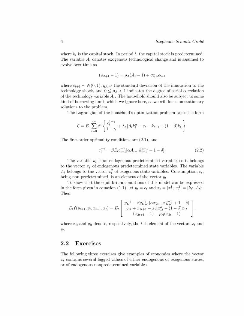
where kt is the capital stock. In period t, the capital stock is predetermined.The variable At denotes exogenous technological change and is assumed to
evolve over time as
(At+1 − 1) = ρA(At − 1) + σηAεt+1
where εt+1 ∼ N (0, 1), ηA is the standard deviation of the innovation to thetechnology shock, and 0 ≤ ρA < 1 indicates the degree of serial correlation
of the technology variable At. The household should also be subject to somekind of borrowing limit, which we ignore here, as we will focus on stationarysolutions to the problem.
The Lagrangian of the household’s optimization problem takes the form
L = E0
∞∑
t=0
βt
{
c1−γt
1 − γ+ λt [Atk
αt − ct − kt+1 + (1− δ)kt]
}
.
The first-order optimality conditions are (2.1), and
c−γt = βEtc
−γt+1[αAt+1k
α−1t+1 + 1 − δ]. (2.2)
The variable kt is an endogenous predetermined variable, so it belongsto the vector x1
t of endogenous predetermined state variables. The variable
At belongs to the vector x2t of exogenous state variables. Consumption, ct,
being non-predetermined, is an element of the vector yt.
To show that the equilibrium conditions of this model can be expressedin the form given in equation (1.1), let yt = ct and xt = [x1
t ; x2t ] = [kt; At]
′.
Then
Etf(yt+1, yt, xt+1, xt) = Et
y−γ1t − βy−γ
1t+1[αx2t+1xα−11t+1 + 1− δ]
y1t + x1t+1 − x2txα1t − (1 − δ)x1t
(x2t+1 − 1)− ρA(x2t − 1)
,
where xit and yit denote, respectively, the i-th element of the vectors xt and
yt.
2.2 Exercises
The following three exercises give examples of economies where the vector
xt contains several lagged values of either endogenous or exogenous states,or of endogenous nonpredetermined variables.

Perturbation Methods, Chapter 2 7
1. Exogenous process with arbitrary AR structure: Suppose that thetechnology shock process instead of following an AR(1) would follow
and AR(l) process with l > 1.2 Show how to write the problem in theform given in equation (1.1). First consider the case l = 2, and thenshow the general case for a finite l.
2. Time-to-Build: Suppose that the production of capital is subject togestation lags. Specifically, in order to build s units of capital available
in period t + J the household has to invest s/J units of goods for Jconsecutive periods starting in period t. The evolution of the capital
stocks is then given by
kt+J = (1 − δ)kt+J−1 + st. (2.3)
Investment in each period is equal to the sum of investments in eachproject initiated in the past J−1 periods including the current period:
it = J−1
J−1∑
i=0
st−i (2.4)
given k0, s−i, i = 0, 1, . . . , J − 1,
where st−i denotes the number of investment projects initiated in pe-riod t − i that will be productive in period t − i + J .
Show how to write the equilibrium conditions that is like the economy
described in the text but for the assumption of time to build. Thenshow how the complete set of equilibrium conditions can be expressed
in the form given in equation (1.1).
3. Habit Formation: Consider a preference specification featuring habitformation. Specifically, assume that instead of deriving utility from
consumption, ct, households derive utility from an object ht given by
ht = ct − θst−1
where st−1 denotes the stock of habit in consumption, which is assumedto evolve over time according to the following law of motion
st = ρst−1 + (1− ρ)ct.
2An autoregressive process of order l, or AR(l), is given by: Xt = A1Xt−1 +A2Xt−2 +. . . + AlXt−l + σεt, where the matrices Ai for i = 1, 2, . . . , l are of size n × n where n isthe length of the vector Xt.
8 Stephanie Schmitt-Grohe
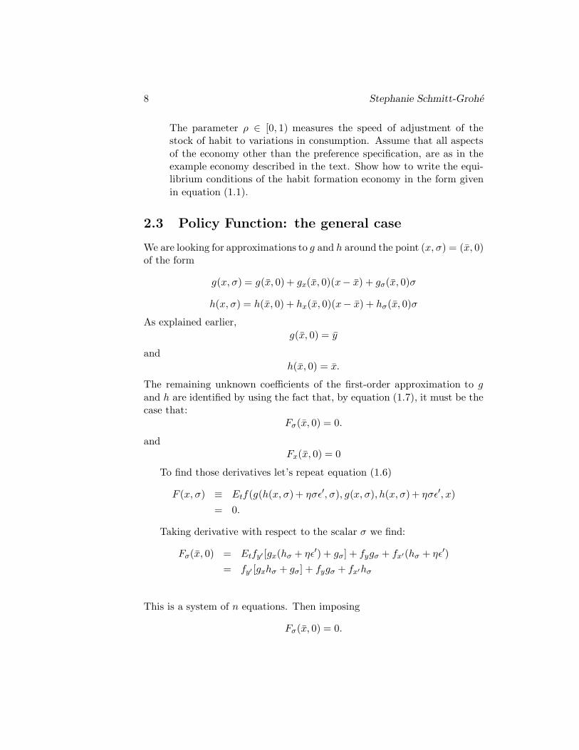
The parameter ρ ∈ [0, 1) measures the speed of adjustment of thestock of habit to variations in consumption. Assume that all aspects
of the economy other than the preference specification, are as in theexample economy described in the text. Show how to write the equi-librium conditions of the habit formation economy in the form given
in equation (1.1).
2.3 Policy Function: the general case
We are looking for approximations to g and h around the point (x, σ) = (x, 0)of the form
g(x, σ) = g(x, 0) + gx(x, 0)(x− x) + gσ(x, 0)σ
h(x, σ) = h(x, 0) + hx(x, 0)(x− x) + hσ(x, 0)σ
As explained earlier,
g(x, 0) = y
and
h(x, 0) = x.
The remaining unknown coefficients of the first-order approximation to g
and h are identified by using the fact that, by equation (1.7), it must be thecase that:
Fσ(x, 0) = 0.
andFx(x, 0) = 0
To find those derivatives let’s repeat equation (1.6)
F (x, σ) ≡ Etf(g(h(x, σ)+ ησε′, σ), g(x, σ), h(x, σ)+ ησε′, x)
= 0.
Taking derivative with respect to the scalar σ we find:
Fσ(x, 0) = Etfy′ [gx(hσ + ηε′) + gσ] + fygσ + fx′(hσ + ηε′)
= fy′ [gxhσ + gσ] + fygσ + fx′hσ
This is a system of n equations. Then imposing
Fσ(x, 0) = 0.
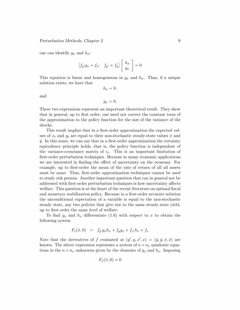
Perturbation Methods, Chapter 2 9
one can identify gσ and hσ :
[
fy′gx + fx′ fy′ + fy
]
[
hσ
gσ
]
= 0
This equation is linear and homogeneous in gσ and hσ . Thus, if a uniquesolution exists, we have that
hσ = 0.
andgσ = 0.
These two expressions represent an important theoretical result. They show
that in general, up to first order, one need not correct the constant term ofthe approximation to the policy function for the size of the variance of the
shocks.This result implies that in a first-order approximation the expected val-
ues of xt and yt are equal to their non-stochastic steady-state values x andy. In this sense, we can say that in a first-order approximation the certainty
equivalence principle holds, that is, the policy function is independent ofthe variance-covariance matrix of εt. This is an important limitation of
first-order perturbation techniques. Because in many economic applicationswe are interested in finding the effect of uncertainty on the economy. Forexample, up to first-order the mean of the rate of return of all all assets
must be same. Thus, first-order approximation techniques cannot be usedto study risk premia. Another important question that can in general not be
addressed with first-order perturbation techniques is how uncertainty affectswelfare. This question is at the heart of the recent literature on optimal fiscal
and monetary stabilization policy. Because in a first-order accurate solutionthe unconditional expectation of a variable is equal to the non-stochastic
steady state, any two policies that give rise to the same steady state yield,up to first-order the same level of welfare.
To find gx and hx differentiate (1.6) with respect to x to obtain thefollowing system
Fx(x, 0) = fy′gxhx + fygx + fx′hx + fx
Note that the derivatives of f evaluated at (y′, y, x′, x) = (y, y, x, x) areknown. The above expression represents a system of n×nx quadratic equa-
tions in the n×nx unknowns given by the elements of gx and hx. Imposing
Fx(x, 0) = 0

10 Stephanie Schmitt-Grohe
the above expression can be written as:
[fx′ fy′ ]
[
I
gx
]
hx = −[fx fy]
[
I
gx
]
Let A = [fx′ fy′ ] and B = −[fx fy]. Note that both A and B are known.
We thus have the following system of n × nx equations:
A
[
Igx
]
hx = B
[
Igx
]
(2.5)
Also, let P the matrix of eigenvectors of the matrix hx such that
hxP = PΛ,
where Λ is diagonal. (The matlab command eig.m produces such a decom-
position). Finally, let
Z ≡
[
I
gx
]
P.
Then the above expression can be written as:
AZΛ = BZ,
We can then map the above problem into a generalized eigenvalue prob-lem. For given n × n matrices A and B, there exists a matrix V and a
diagonal matrix D such that (using the matlab command [V,D]=eig(B,A)):
A[V1 V2]
[
D11 ∅∅ D22
]
= B[V1 V2]
Assume, without of loss of generality, that all the eigenvalues of D11 havemodulus less than unity. Then we have:
Λ = D11
[
Igx
]
P = V1 =
[
V11
V12
]
So that
hx = V11D11V−111
and
gx = V12V−111
Perturbation Methods, Chapter 2 11
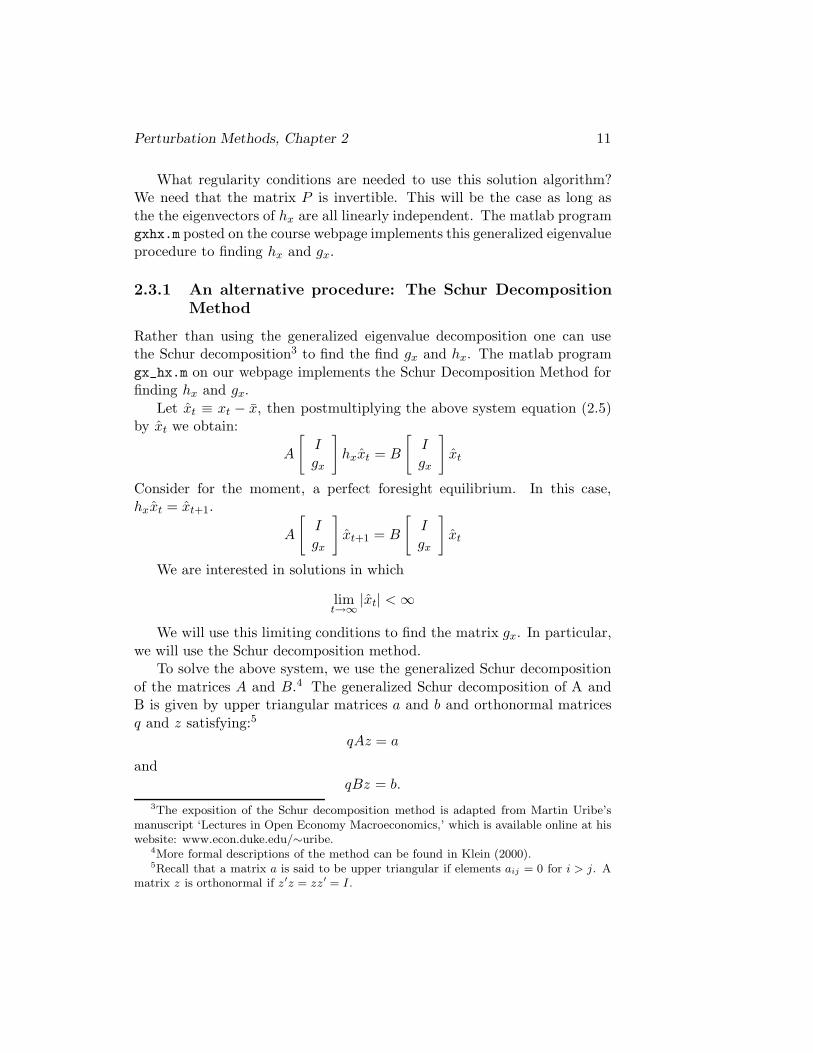
What regularity conditions are needed to use this solution algorithm?We need that the matrix P is invertible. This will be the case as long as
the the eigenvectors of hx are all linearly independent. The matlab programgxhx.m posted on the course webpage implements this generalized eigenvalueprocedure to finding hx and gx.
2.3.1 An alternative procedure: The Schur Decomposition
Method
Rather than using the generalized eigenvalue decomposition one can usethe Schur decomposition3 to find the find gx and hx. The matlab program
gx_hx.m on our webpage implements the Schur Decomposition Method forfinding hx and gx.
Let xt ≡ xt − x, then postmultiplying the above system equation (2.5)by xt we obtain:
A
[
I
gx
]
hxxt = B
[
I
gx
]
xt
Consider for the moment, a perfect foresight equilibrium. In this case,hxxt = xt+1.
A
[
I
gx
]
xt+1 = B
[
I
gx
]
xt
We are interested in solutions in which
limt→∞
|xt| < ∞
We will use this limiting conditions to find the matrix gx. In particular,
we will use the Schur decomposition method.To solve the above system, we use the generalized Schur decomposition
of the matrices A and B.4 The generalized Schur decomposition of A andB is given by upper triangular matrices a and b and orthonormal matrices
q and z satisfying:5
qAz = a
and
qBz = b.
3The exposition of the Schur decomposition method is adapted from Martin Uribe’smanuscript ‘Lectures in Open Economy Macroeconomics,’ which is available online at hiswebsite: www.econ.duke.edu/∼uribe.
4More formal descriptions of the method can be found in Klein (2000).5Recall that a matrix a is said to be upper triangular if elements aij = 0 for i > j. A
matrix z is orthonormal if z′z = zz′ = I .
12 Stephanie Schmitt-Grohe
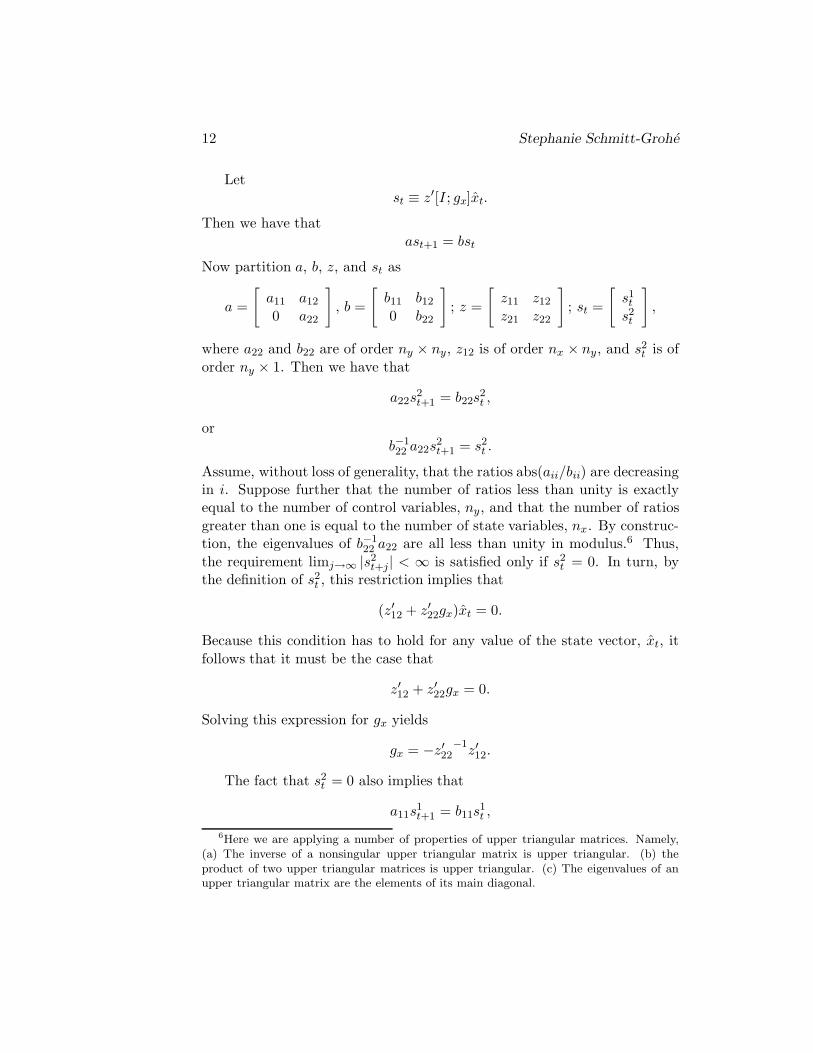
Letst ≡ z′[I ; gx]xt.
Then we have that
ast+1 = bst
Now partition a, b, z, and st as
a =
[
a11 a12
0 a22
]
, b =
[
b11 b12
0 b22
]
; z =
[
z11 z12
z21 z22
]
; st =
[
s1t
s2t
]
,
where a22 and b22 are of order ny × ny, z12 is of order nx × ny, and s2t is of
order ny × 1. Then we have that
a22s2t+1 = b22s
2t ,
orb−122
a22s2t+1 = s2
t .
Assume, without loss of generality, that the ratios abs(aii/bii) are decreasingin i. Suppose further that the number of ratios less than unity is exactlyequal to the number of control variables, ny, and that the number of ratios
greater than one is equal to the number of state variables, nx. By construc-tion, the eigenvalues of b−1
22a22 are all less than unity in modulus.6 Thus,
the requirement limj→∞ |s2t+j| < ∞ is satisfied only if s2
t = 0. In turn, bythe definition of s2
t , this restriction implies that
(z′12 + z′22gx)xt = 0.
Because this condition has to hold for any value of the state vector, xt, it
follows that it must be the case that
z′12 + z′22gx = 0.
Solving this expression for gx yields
gx = −z′22
−1z′12.
The fact that s2t = 0 also implies that
a11s1t+1 = b11s
1t ,
6Here we are applying a number of properties of upper triangular matrices. Namely,(a) The inverse of a nonsingular upper triangular matrix is upper triangular. (b) theproduct of two upper triangular matrices is upper triangular. (c) The eigenvalues of anupper triangular matrix are the elements of its main diagonal.
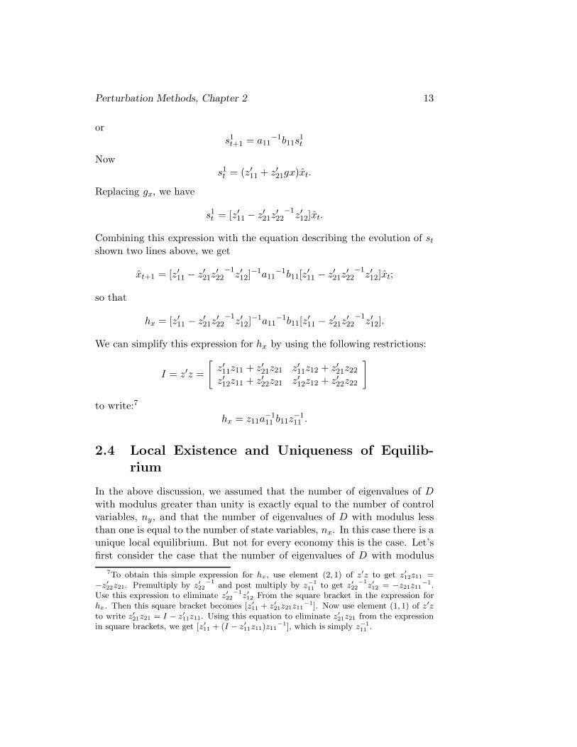
Perturbation Methods, Chapter 2 13
or
s1t+1 = a11
−1b11s1t
Now
s1t = (z′11 + z′21gx)xt.
Replacing gx, we have
s1t = [z′11 − z′21z
′
22
−1z′12]xt.
Combining this expression with the equation describing the evolution of st
shown two lines above, we get
xt+1 = [z′11 − z′21z′
22
−1z′12]
−1a11−1b11[z
′
11 − z′21z′
22
−1z′12]xt;
so that
hx = [z′11 − z′21z′
22
−1z′12]
−1a11−1b11[z
′
11 − z′21z′
22
−1z′12].
We can simplify this expression for hx by using the following restrictions:
I = z′z =
[
z′11z11 + z′21z21 z′11z12 + z′21z22
z′12z11 + z′22z21 z′12z12 + z′22z22
]
to write:7
hx = z11a−111 b11z
−111 .
2.4 Local Existence and Uniqueness of Equilib-
rium
In the above discussion, we assumed that the number of eigenvalues of D
with modulus greater than unity is exactly equal to the number of controlvariables, ny, and that the number of eigenvalues of D with modulus less
than one is equal to the number of state variables, nx. In this case there is aunique local equilibrium. But not for every economy this is the case. Let’s
first consider the case that the number of eigenvalues of D with modulus
7To obtain this simple expression for hx, use element (2, 1) of z′z to get z′
12z11 =−z′
22z21. Premultiply by z′
22
−1and post multiply by z−1
11to get z′
22
−1z′
12 = −z21z11−1.
Use this expression to eliminate z′
22
−1z′
12 From the square bracket in the expression forhx. Then this square bracket becomes [z′
11 + z′
21z21z11−1]. Now use element (1, 1) of z′z
to write z′
21z21 = I − z′
11z11. Using this equation to eliminate z′
21z21 from the expressionin square brackets, we get [z′
11 + (I − z′
11z11)z11−1], which is simply z−1
11.
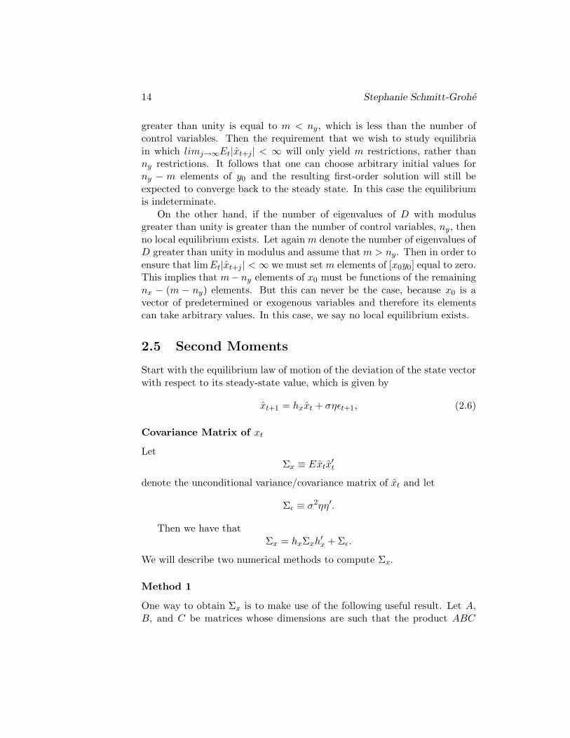
14 Stephanie Schmitt-Grohe
greater than unity is equal to m < ny, which is less than the number ofcontrol variables. Then the requirement that we wish to study equilibria
in which limj→∞Et|xt+j| < ∞ will only yield m restrictions, rather thanny restrictions. It follows that one can choose arbitrary initial values forny − m elements of y0 and the resulting first-order solution will still be
expected to converge back to the steady state. In this case the equilibriumis indeterminate.
On the other hand, if the number of eigenvalues of D with modulusgreater than unity is greater than the number of control variables, ny, then
no local equilibrium exists. Let again m denote the number of eigenvalues ofD greater than unity in modulus and assume that m > ny. Then in order to
ensure that limEt|xt+j| < ∞ we must set m elements of [x0y0] equal to zero.This implies that m− ny elements of x0 must be functions of the remaining
nx − (m − ny) elements. But this can never be the case, because x0 is avector of predetermined or exogenous variables and therefore its elementscan take arbitrary values. In this case, we say no local equilibrium exists.
2.5 Second Moments
Start with the equilibrium law of motion of the deviation of the state vector
with respect to its steady-state value, which is given by
xt+1 = hxxt + σηεt+1, (2.6)
Covariance Matrix of xt
Let
Σx ≡ Extx′
t
denote the unconditional variance/covariance matrix of xt and let
Σε ≡ σ2ηη′.
Then we have that
Σx = hxΣxh′
x + Σε.
We will describe two numerical methods to compute Σx.
Method 1
One way to obtain Σx is to make use of the following useful result. Let A,B, and C be matrices whose dimensions are such that the product ABC
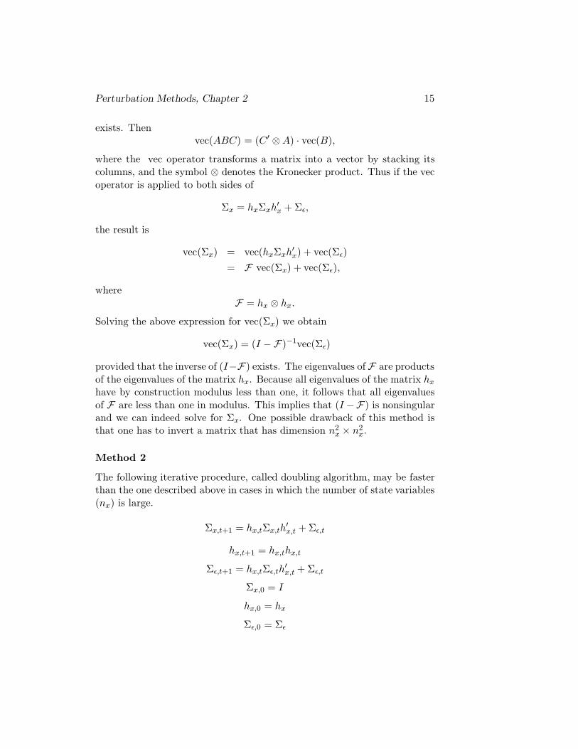
Perturbation Methods, Chapter 2 15
exists. Thenvec(ABC) = (C′ ⊗ A) · vec(B),
where the vec operator transforms a matrix into a vector by stacking itscolumns, and the symbol ⊗ denotes the Kronecker product. Thus if the vec
operator is applied to both sides of
Σx = hxΣxh′
x + Σε,
the result is
vec(Σx) = vec(hxΣxh′
x) + vec(Σε)
= F vec(Σx) + vec(Σε),
where
F = hx ⊗ hx.
Solving the above expression for vec(Σx) we obtain
vec(Σx) = (I − F )−1vec(Σε)
provided that the inverse of (I−F ) exists. The eigenvalues of F are products
of the eigenvalues of the matrix hx. Because all eigenvalues of the matrix hx
have by construction modulus less than one, it follows that all eigenvalues
of F are less than one in modulus. This implies that (I −F ) is nonsingularand we can indeed solve for Σx. One possible drawback of this method isthat one has to invert a matrix that has dimension n2
x × n2x.
Method 2
The following iterative procedure, called doubling algorithm, may be fasterthan the one described above in cases in which the number of state variables
(nx) is large.
Σx,t+1 = hx,tΣx,th′
x,t + Σε,t
hx,t+1 = hx,thx,t
Σε,t+1 = hx,tΣε,th′
x,t + Σε,t
Σx,0 = I
hx,0 = hx
Σε,0 = Σε

16 Stephanie Schmitt-Grohe
Other second moments
Once the covariance matrix of the state vector, xt has been computed, it
is easy to find other second moments of interest. Consider for instance thecovariance matrix Extx
′
t−j for j > 0. Let µt = σηεt.
Extx′
t−j = E[hjxxt−j +
j−1∑
k=0
hkxµt−k]x′
t−j
= hjxExt−jx
′
t−j
= hjxΣx
Similarly, consider the variance covariance matrix of linear combinations of
the state vector xt. For instance, the co-state, or control vector yt is givenby yt = y + gx(xt − x), which we can write as: yt = gxxt. Then
Eyty′
t = Egxxtx′
tg′
x
= gx[Extx′
t]g′
x
= gxΣxg′x
and, more generally,
Eyty′
t−j = gx[Extx′
t−j]g′
x
= gxhjxΣxg′x,
for j ≥ 0.
2.6 Impulse Response Functions
The impulse response to a variable, say zt in period t + j to an impulse inperiod t is defined as:
IR(zt+j) ≡ Etzt+j − Et−1zt+j
The impulse response function traces the expected behavior of the systemfrom period t on given information available in period t, relative to what
was expected at time t − 1. Using the law of motion Etxt+1 = hxxt for thestate vector, letting x denote the innovation to the state vector in period 0,
that is, x = ησε0, and applying the law of iterated expectations we get thatthe impulse response of the state vector in period t is given by
IR(xt) ≡ E0xt − E−1xt = htx[x0 − E−1x0] = ht
x[ησε0] = htxx; t ≥ 0.
The response of the vector of controls yt is given by
IR(yt) = gxhtxx.

Perturbation Methods, Chapter 2 17
2.7 Matlab Code For Linear Perturbation Meth-
ods
Martin Uribe and I have written a suite of programs that are posted onwww.columbia.edu/~mu2166. The program gxhx.m computes the matrices
gx and hx using the generalized eigenvalue method. The program mom.mcomputes second moments. The program ir.m computes impulse response
functions.There are a number of other programs out there to compute the ma-
trices gx and hx. For example, Paul Klein of the University of West-ern Ontario has written Matlab programs that compute the matrices hx
and gx given A, B, and nx, using the Schur decomposition methods that
we also discussed in the lecture notes (but not in class). To use this al-ternative method one needs to use a set of programs consisting of three
files, solab.m, qzswitch.m, and qzdiv.m, which are available on Paul Klein’swebsite, http://www.ssc.uwo.ca/economics/faculty/klein/. The programs
qzswitch.m and qzdiv.m were created by Chris Sims of Princeton Univer-sity. The files qzswitch.m and qzdiv.m are needed to arrive at a Schur
decomposition in which the ratios abs(aii/bii) are decreasing in i. The pro-gram solab.m, then uses the matrices a and b to find the matrices gx and
hx.
2.8 Exercises
The following exercises ask you to apply first-order perturbation methodsto numerically analyze the real business cycle model.
1. How does depreciation affect the response of consumption to a positivetechnology shock? Plot the initial response of consumption to a one
percent increase in At as a function of δ. Consider values of δ between0 and 1. Give intuition for your findings. (Use the set of programs forthe neoclassical growth model that are posted on our Second-Order
Approximation website.)
2. How does the persistence of the technology shock affect the response ofhours? Use the neoclassical growth model we studied earlier. However,
now assume that labor supply is endogenous. In particular, the utilityfunction now is given by
u(c, h) =[c(1− ht)
ξ]1−γ − 1
1 − γ
18 Stephanie Schmitt-Grohe
and that the production function is Cobb Douglas in capital and hours.To calibrate this economy impose that in steady state households
spend 20 percent of their time working (hss = 0.2) and that the laborshare in value added is 70 percent (1 − α) = 0.7. Assume that therate of depreciation is 10 percent per year. Find the steady state of
the economy and the parameter value for ξ. Then plot the initial re-sponse of hours to a one percent increase in the technology shock as a
function of the serial correlation coefficient ρA. Provide intuition foryour findings.
3. How does the value of the Frisch elasticity of labor supply affect (a)
the volatility of hours relative to that of output; (b) the correlationbetween hours and output; (c) the correlation between hours and laborproductivity; (d) the correlation between output and labor productiv-
ity;

Chapter 3
Second-Order Perturbation
Methods
Most models used in modern macroeconomics are too complex to allow forexact solutions. For this reason, researchers have appealed to numerical
approximation techniques. One popular and widely used approximationtechnique that we studied in the previous lecture is a first-order perturba-
tion method delivering a linear approximation to the policy function. Onereason for the popularity of first-order perturbation techniques is that they
do not suffer from the ’curse of dimensionality.’ That is, problems with alarge number of state variables can be handled without much computational
demands. Because models that are successful in accounting for many aspectsof observed business cycles are bound to be large, this advantage of perturba-tion techniques is of particular importance for policy evaluation. However,
first-order approximation techniques suffer from serious limitations whenapplied to welfare evaluation. The problem is that when welfare is evalu-
ated using a first-order approximation to the equilibrium laws of motion ofendogenous variables, some second- and higher-order terms of the equilib-
rium welfare function are omitted while others are included. Consequently,the resulting criterion is inaccurate to order two or higher. This inaccuracy
may result in spurious welfare rankings. For instance, in a recent paperJinill Kim and Sunghyun Kim show that in a simple two-agent economy, a
welfare comparison based on an evaluation of the utility function using alinear approximation to the policy function may yield the erroneous resultthat welfare is higher under autarky than under full risk sharing. Similarly,
Tesar (1995) reports that the welfare gains from risksharing a negative insome cases. Again this erroneous finding is due to the fact that she uses
19

20 Stephanie Schmitt-Grohe
first order approximations to the decision rules. If welfare were directly ap-proximated to first order then, as we saw in the previous class, all policies
that imply the same non-stochastic steady state will give rise to the samelevel of welfare up to first-order. So, for example, the welfare gains fromrisk sharing should be zero.
In general, to be able to measure welfare gains from different stabiliza-tion policies or from different risk sharing arrangements requires a correct
second-order approximation of the equilibrium welfare function, which inturn requires a second-order approximation to the policy function. This is
what we will study in this chapter. First, we derive an accurate second-orderapproximation to the solution of discrete-time rational expectations models
whose equilibrium conditions can be expressed as in equation (1.1).
In today’s lecture we will show that for any model belonging to this
general class, the coefficients on the terms linear and quadratic in the statevector in a second-order expansion of the decision rule are independent of the
volatility of the exogenous shocks. In other words, these coefficients must bethe same in the stochastic and the deterministic versions of the model. Thus,
up to second order, the presence of uncertainty affects only the constant termof the decision rules. But the fact that only the constant term is affected by
the presence of uncertainty is by no means inconsequential. For it impliesthat up to second order the unconditional mean of endogenous variablescan in general be significantly different from their non-stochastic steady
state values. Thus, second-order approximation methods can in principlecapture important effects of uncertainty on, for example, average rate of
return differentials across assets with different risk characteristics or on theaverage level of consumer welfare. An additional advantage of higher-order
perturbation methods is that like their first-order counterparts, they do notsuffer from the curse of dimensionality. This is because given the first-order
approximation to the policy function, finding the coefficients of a second-order approximation simply entails solving a system of linear equations.
3.1 Finding the second-order approximation
The second-order approximations to g and h around the point (x, σ) = (x, 0)are of the form
[g(x, σ)]i = [g(x, 0)]i + [gx(x, 0)]ia[(x− x)]a + [gσ(x, 0)]i[σ]
+1
2[gxx(x, 0)]iab[(x − x)]a[(x − x)]b
Perturbation Methods, Chapter 3 21
+1
2[gxσ(x, 0)]ia[(x − x)]a[σ]
+1
2[gσx(x, 0)]ia[(x − x)]a[σ]
+1
2[gσσ(x, 0)]i[σ][σ]
[h(x, σ)]j = [h(x, 0)]j + [hx(x, 0)]ja[(x− x)]a + [hσ(x, 0)]j[σ]
+1
2[hxx(x, 0)]jab[(x − x)]a[(x − x)]b
+1
2[hxσ(x, 0)]ja[(x− x)]a[σ]
+1
2[hσx(x, 0)]ja[(x− x)]a[σ]
+1
2[hσσ(x, 0)]j[σ][σ],
where i = 1, . . . , ny, a, b = 1, . . . , nx, and j = 1, . . . , nx.Here we are using a notation suggested by Collard and Juillard (2001a).
So, for example, [fy′ ]iα is the (i, α) element of the derivative of f with re-
spect to y′. The derivative of f with respect to y′ is an n × ny matrix.
Therefore, [fy′ ]iα is the element of this matrix located at the intersection
of the i-th row and α-th column. Also, for example, [fy′ ]iα[gx]
αβ [hx]βj =
∑ny
α=1
∑nx
β=1
∂f i
∂y′α∂gα
∂xβ∂hβ
∂xj .
The unknowns of this expansion are [gxx]iab, [gxσ]ia, [gσx]ia, [gσσ]i, [hxx]jab,
[hxσ]ja, [hσx]ja, [hσσ ]j, where we have omitted the argument (x, 0). These
coefficients can be identified by taking the derivative of F (x, σ) with respectto x and σ twice and evaluating them at (x, σ) = (x, 0). By the arguments
provided earlier, these derivatives must be zero. Specifically, we use Fxx(x, 0)to identify gxx(x, 0) and hxx(x, 0). That is,1
[Fxx(x, 0)]ijk =(
[fy′y′ ]iαγ [gx]
γδ [hx]δk + [fy′y]
iαγ [gx]
γk + [fy′x′ ]iαδ[hx]
δk + [fy′x]iαk
)
[gx]αβ [hx]
βj
+[fy′ ]iα[gxx]
αβδ[hx]δk[hx]βj
+[fy′ ]iα[gx]αβ [hxx]βjk
+(
[fyy′ ]iαγ[gx]γδ [hx]
δk + [fyy]
iαγ [gx]
γk + [fyx′ ]iαδ[hx]δk + [fyx]iαk
)
[gx]αj
+[fy]iα[gxx]
αjk
1At this point, an additional word about notation is in order. Take for example theexpression [fy′y′ ]iαγ. Note that fy′y′ is a three dimensional array with n rows, ny columns,and ny pages. Then [fy′y′]iαγ denotes the element of fy′y′ located at the intersection ofrow i, column α and page γ.
22 Stephanie Schmitt-Grohe
+(
[fx′y′ ]iβγ[gx]γδ [hx]δk + [fx′y]
iβγ [gx]
γk + [fx′x′ ]iβδ[hx]δk + [fx′x]iβk
)
[hx]βj
+[fx′ ]iβ[hxx]βjk
+[fxy′ ]ijγ [gx]
γδ [hx]
δk + [fxy]
ijγ [gx]γk + [fxx′ ]ijδ[hx]
δk + [fxx]ijk
= 0; i = 1, . . .n, j, k, β, δ = 1, . . .nx; α, γ = 1, . . .ny.
Since we know the derivatives of f as well as the first derivatives of g and hevaluated at (y′, y, x′, x) = (y, y, x, x), it follows that the above expression
represents a system of n × nx × nx linear equations in the n × nx × nx
unknowns given by the elements of gxx and hxx.
Similarly, gσσ and hσσ can be obtained by solving the linear systemFσσ(x, 0) = 0. More explicitly,
[Fσσ(x, 0)]i = [fy′ ]iα[gx]
αβ [hσσ]β
+[fy′y′ ]iαγ [gx]
γδ [η]δξ[gx]
αβ [η]βφ[I ]φξ
+[fy′x′ ]iαδ[η]δξ[gx]αβ [η]βφ[I ]φξ
+[fy′ ]iα[gxx]
αβδ[η]δξ[η]βφ[I ]φξ
+[fy′ ]iα[gσσ]α (3.1)
+[fy]iα[gσσ]α
+[fx′ ]iβ [hσσ]β
+[fx′y′ ]iβγ [gx]
γδ [η]δξ[η]βφ[I ]φξ
+[fx′x′ ]iβδ[η]δξ[η]βφ[I ]φξ= 0; i = 1, . . . , n; α, γ = 1, . . . , ny; β, δ = 1, . . . , nx; φ, ξ = 1, . . . , nε.
This is a system of n linear equations in the n unknowns given by the
elements of gσσ and hσσ .Finally, we show that the cross derivatives gxσ and hxσ are equal to zero
when evaluated at (x, 0). We write the system Fσx(x, 0) = 0 taking into
account that all terms containing either gσ or hσ are zero at (x, 0). Thenwe have,
[Fσx(x, 0)]ij = [fy′ ]iα[gx]
αβ [hσx]βj + [fy′ ]
iα[gσx]
αγ [hx]γj + [fy]
iα[gσx]
αj + [fx′ ]iβ[hσx]βj
= 0; i = 1, . . .n; α = 1, . . . , ny; β, γ, j = 1, . . . , nx. (3.2)
This is a system of n × nx equations in the n × nx unknowns given by theelements of gσx and hσx. But clearly, the system is homogeneous in the
unknowns. Thus, if a unique solution exists, it is given by
gσx = 0

Perturbation Methods, Chapter 3 23
andhσx = 0.
These equations represent an important theoretical result. They show that
in general, up to second-order, the coefficients of the policy function on theterms that are linear in the state vector do not depend on the size of the
variance of the underlying shocks.This result implies that the second-order approximation to the policy
function of a stochastic model belonging to the general class given in equa-
tion (1.1) differs from that of its non-stochastic counterpart only in a con-stant term given by 1
2gσσσ2 for the control vector yt and by 1
2hσσσ2 for the
state vector xt.As we stressed above what is simple about finding the second order terms
of the functions g and h that it only involves linear operations. This suggeststhat one can postulate the problem in matrix form. This is what is done,
numerically, in the programs gxx hxx.m and gss hss.m.
3.2 Implementing Second-Order Methods
3.2.1 Computing the derivatives of f
Computing the derivatives of f , particulary, second derivatives, can be
daunting task. It is almost impossible to do this by hand for any but themost simple of models. And most of us would get lost in algebra mistakes.
So clearly one must resort to the computer for finding those derivates. Hereone has two options. One is to try to find the numerical derivatives. But
this is not the way we approach the problem in Schmitt-Grohe and Uribe(JEDC 2004). We instead make use of the capabilities of symbolic math soft-
ware. The particular one we use is the MATLAB Toolbox Symbolic Math.Symbolic Math can handle analytical derivatives. We wrote programs, thatcompute the analytical derivatives of f and evaluate them at the steady
state. The program anal deriv.m computes analyltical derivatives of f andthe program num eval.m evaluates the analytical derivatives of f . You can
check these programs out on the Second-Order Approximation website.
3.2.2 Which steady state to approximate around
In general, the second-order method exposited here can be used to computewelfare in the neighborhood of an arbitrary steady state.
However, in a monetary or fiscal policy stabilization problem, the steadystate of the economy depends on the assumed policy. Suppose we wish

24 Stephanie Schmitt-Grohe
to evaluate the welfare consequences of alternative monetary stabilizationpolicies with the objective to pick the best of those. In such an exercise one
can, in principle, freely pick the steady state level of inflation around whichthe economy should be stabilized. For example, one could study the case inwhich inflation is stablized around, say 5 percent of inflation per year. But if,
in the particular model studied the optimal inflation rate in the steady stateis, say 0 percent per year, such a research strategy, may lead to the following
problem. The benevolent policy maker may want to use stabilization policyto get the mean of inflation down, that is down from 5 percent to something
closer to 0 percent. And the welfare gains from influencing the mean may belarger than stabilizing the economy around the deterministic steady state.
For this reason, the accuracy of the approximation may be poor. Therefore,if one uses second-order approximation methods to find the best among a
class of suboptimal policies, one should approximate the economy aroundthe Ramsey steady state.
In other contexts, that is when one is not using the second-order approx-
imation to find the best constrained policy, the perturbation method can beapplied successfully to any arbitrary non-stochastic steady state. Say, if we
want to characterize risk premia, then the accuracy of the second-order per-turbation method should be independent of the Ramsey optimality of the
point around which the solution is approximated.
3.2.3 How to construct second-order accurate time series
Suppose one wishes to simulate a time series path of the approximate solu-
tion for xt and yt. One possibility of proceeding is to start with an initialvalue of the state, say x0, and then to use the second-order approximation
to the function h iteratively to produce a time path. That is, iterate on:(Assume w.l.g. that the steady state value of x is zero.)
xi1 = hi
xx0 + x′
0hixxx0 + σηiε1.
In this way one can obtain time series for xt and yt conditional upon a partic-ular value of x0. This procedure is second-order accurate, but it introduces
some higher-order terms into the expansion. These extra higher order-termsdo not in general increase accuracy of the approximation as they do not cor-
respoind to higer-order coefficients in a Taylor expansion. In practise theyoften lead to explosive time paths for xt. To see what goes wrong let (this
example is taken from Kim, Kim, Schaumburg, and Sims)
xt+1 = ρxt + αx2t + εt+1; 0 < ρ < 1
Perturbation Methods, Chapter 3 25
Note that this system has two steady states. One at x = 0 and the other atx = (1− ρ)/α. Linearizing ths system around x = x yields:
xt+1 = ρxt + εt+1
Given the assumpmtion that ρ < 1, this system is sstable in the neigh-
borhood of x = 0. But the sysstem is unstable in the neighborhood ofx = (1− ρ)/α. Thus, once xt > (1− ρ)/α, the system will diverge.
Therefore, one should choose among the second-order accurate expan-sions the o ne that implies stability. A stable solution can be obtained by
‘PRUNING’ (a term coined by Chris Sims) out the the extraneous higher-order terms in each iteration by computing the projections of the second-
order terms based on a first-order expansions. LLet xf
t be the first-order iterate of xt given some x0., that is , xf0 = x0,
and let xst be the second-order iterate of xt given x0 and set xs
0 = 0. Then
definexf
t+1= hxxf
t + σηεt+1
and
xist+1 = hi
xxst +
1
2xf ′
t hixxxf
t +1
2+ hi
σσσ2
The program simu 2nd.m posted on our Second Order website constructs
such time series.
3.2.4 How to compute unconditional first moments
First note that the variance of either xt or yt are correct to second-order
accuracy when computed from the first-order approximation alone. (Thatis, you can use the program mom.m to find the second-oder accurate second-moments.) Then, suppose that the unconditional expectation of xt exists,
we can approximate this from its law of motion (assume without loss ofgenerality that xSS = 0:
xit+1 ≈ hi
xxt +1
2x′
thixxxt +
1
2hi
σσσ2 + σηiεt+1
Note that eh scalarx′
thixxxt = x′
t ⊗ x′
tvec(hixx)
and that Ex′
t ⊗ x′
t = vec(Σx)′. We then have that :
Ex′
thixxxt = Ex′
t ⊗ x′
tvec(hixx)
= (vec(Σx))′vec(hi
xx)

26 Stephanie Schmitt-Grohe
It follows that
Ext+1 = hxExt +
vec(h1xx)
′
vec(h2xx)
′
. . .
vec(hnxxx)′
vec(Σx)/2 +1
2hσσσ2
Ext = (I − hx)−1
vec(h1xx)
′
vec(h2xx)
′
. . .vec(hnx
xx)′
vec(Σx)/2 +1
2hσσσ2
The program unconditional means.m computes unconditioanl means.
3.3 Second-order accurate welfare approximations
Suppose we wish to evaluate the welfare consequences of alternative mon-
etary policy arrangements. How should welfare be measured? Welfare isdefined as the present dicounted value of lifetime utility. One could mea-sure this either using the conditional expectation of lifetime utility or the
unconditional expection:
Conditional Welfare Measures
Let Vt denote the time t value of the present disounted value of lifetimeutility. For example, in the case of the economy desribed in section 2.1
above we have:
Vt ≡ Et
∞∑
j=0
βjU(ct+j)
What we are looking for is a second-order accurate approximation to
Vt. At first instinct one may think that one way to obtain Vt is to find asecond-order accurate time series for ct and then just use the sample mean
of say 1000 simulated paths for∑T
t=0 βtU(ct) for some rather large T . Thisway of proceeding is however unneccarily cumbersome and may introduce
some errors stemming from the fact that one uses a sample path. Insteadthe way to proceed is to write Vt recursively as:
Vt = U(ct) + βEtVt+1
Then add this expression the vector valued function f and make Vt anelement of the vector of endogenous non-predetermined variables yt. In this

Perturbation Methods, Chapter 3 27
way, once one has computed second-order approximations to the function g,one has the second-order approximation of Vt in hand. The idea is that we
can express Vt as some non-linear function of the state vector xt and of thescalar parameter σ, that is,
Vt = gV (xt, σ)
where, here the function gV is just one element of the function g that we
introduced earlier. It maps Rnx ×R+ into R. And by making Vt one row off , we can obtain the second-order accurate approximation to the function
gV .
Clearly, the level of welfare will depend on the initial state being consid-ered, that is, on the value of the state vector xt. Depending on the particularquestion one would like to address, one may consider a number of relevant
initial values for xt and average over those to obtain an average value ofconditional welfare levels.
Welfare cost measures
Often in comparing alternative policies that are consistent with the same
non-stochastic steady state equilibrium, one would like to put the welfaredifferences into perspective. Saying that the welfare of policy A is, say, 255.3,
and that associated with policy B is, say 248.7, only tells us that policyA welfare dominates policy B. But often we are interested in asking howmuch better policy A is than policy B. One way of quantifying these welfare
differences is to ask what percentage of the consumption stream associatedwith policy A, households are willing to give to be as well off, under policy
A as under policy B. Let cAt the contingent plan for consumption associated
with policy A and cBt the contingent plan for consumption associated with
policy B. We can then implicitly define the welfare cost of adoptiong policyB rather than policy A as the value of λ such that
V Bt = Et
∞∑
t=0
βtU(cAt (1− λ))
Suppose the utility function is of the form:
U(c) =c1−γ
1 − γ
with 0 < γ < 1
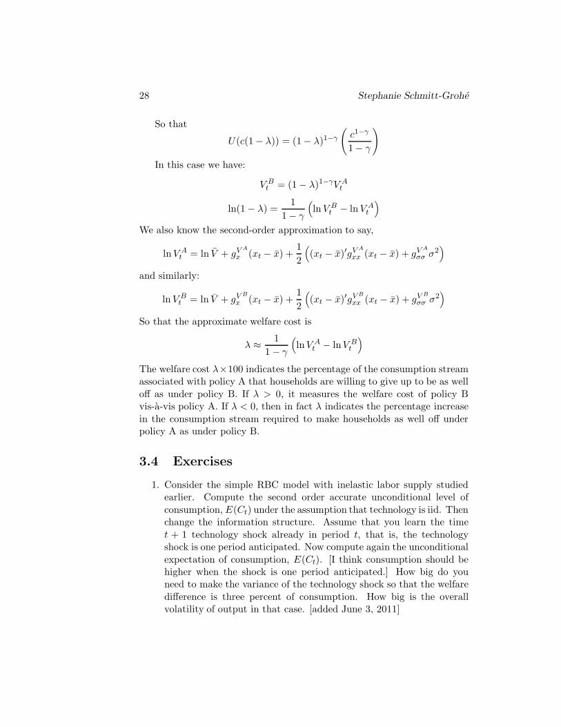
28 Stephanie Schmitt-Grohe
So that
U(c(1− λ)) = (1− λ)1−γ
(
c1−γ
1− γ
)
In this case we have:
V Bt = (1− λ)1−γV A
t
ln(1− λ) =1
1− γ
(
ln V Bt − ln V A
t
)
We also know the second-order approximation to say,
ln V At = ln V + gV A
x (xt − x) +1
2
(
(xt − x)′gV A
xx (xt − x) + gV A
σσ σ2)
and similarly:
ln V Bt = ln V + gV B
x (xt − x) +1
2
(
(xt − x)′gV B
xx (xt − x) + gV B
σσ σ2)
So that the approximate welfare cost is
λ ≈1
1 − γ
(
lnV At − lnV B
t
)
The welfare cost λ×100 indicates the percentage of the consumption streamassociated with policy A that households are willing to give up to be as well
off as under policy B. If λ > 0, it measures the welfare cost of policy Bvis-a-vis policy A. If λ < 0, then in fact λ indicates the percentage increase
in the consumption stream required to make households as well off underpolicy A as under policy B.
3.4 Exercises
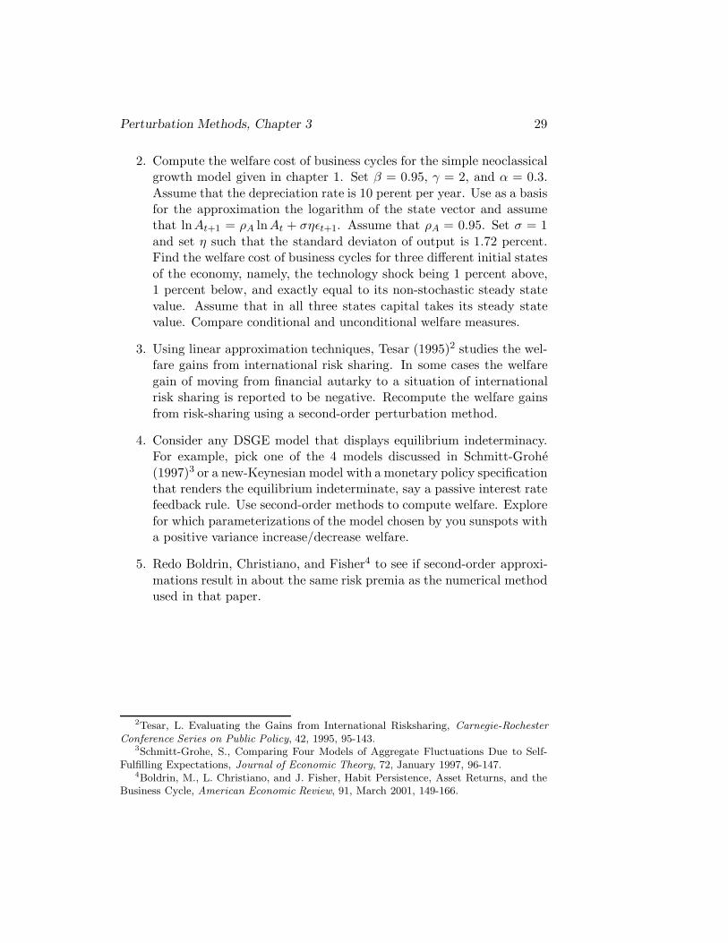
1. Consider the simple RBC model with inelastic labor supply studiedearlier. Compute the second order accurate unconditional level of
consumption, E(Ct) under the assumption that technology is iid. Thenchange the information structure. Assume that you learn the time
t + 1 technology shock already in period t, that is, the technologyshock is one period anticipated. Now compute again the unconditional
expectation of consumption, E(Ct). [I think consumption should behigher when the shock is one period anticipated.] How big do youneed to make the variance of the technology shock so that the welfare
difference is three percent of consumption. How big is the overallvolatility of output in that case. [added June 3, 2011]
Perturbation Methods, Chapter 3 29
2. Compute the welfare cost of business cycles for the simple neoclassicalgrowth model given in chapter 1. Set β = 0.95, γ = 2, and α = 0.3.
Assume that the depreciation rate is 10 perent per year. Use as a basisfor the approximation the logarithm of the state vector and assumethat lnAt+1 = ρA lnAt + σηεt+1. Assume that ρA = 0.95. Set σ = 1
and set η such that the standard deviaton of output is 1.72 percent.Find the welfare cost of business cycles for three different initial states
of the economy, namely, the technology shock being 1 percent above,1 percent below, and exactly equal to its non-stochastic steady state
value. Assume that in all three states capital takes its steady statevalue. Compare conditional and unconditional welfare measures.
3. Using linear approximation techniques, Tesar (1995)2 studies the wel-fare gains from international risk sharing. In some cases the welfare
gain of moving from financial autarky to a situation of internationalrisk sharing is reported to be negative. Recompute the welfare gains
from risk-sharing using a second-order perturbation method.
4. Consider any DSGE model that displays equilibrium indeterminacy.For example, pick one of the 4 models discussed in Schmitt-Grohe
(1997)3 or a new-Keynesian model with a monetary policy specificationthat renders the equilibrium indeterminate, say a passive interest ratefeedback rule. Use second-order methods to compute welfare. Explore
for which parameterizations of the model chosen by you sunspots witha positive variance increase/decrease welfare.
5. Redo Boldrin, Christiano, and Fisher4 to see if second-order approxi-
mations result in about the same risk premia as the numerical methodused in that paper.
2Tesar, L. Evaluating the Gains from International Risksharing, Carnegie-Rochester
Conference Series on Public Policy, 42, 1995, 95-143.3Schmitt-Grohe, S., Comparing Four Models of Aggregate Fluctuations Due to Self-
Fulfilling Expectations, Journal of Economic Theory, 72, January 1997, 96-147.4Boldrin, M., L. Christiano, and J. Fisher, Habit Persistence, Asset Returns, and the
Business Cycle, American Economic Review, 91, March 2001, 149-166.

30 Stephanie Schmitt-Grohe

Chapter 4
N-th Perturbation Methods
It is straightforward to apply the method described thus far to finding higherthan second-order approximations to the policy function. For example, given
the first- and second-order terms of the Taylor expansions of h and g, thethird-order terms can be identified by solving a linear system of equations.
More generally, one can construct sequentially the nth-order approximationof the policy function by solving a linear system of equations whose (known)
coefficients are the lower-order terms and the derivatives up to order n of fevaluated at (y′, y, x′, x) = (y, y, x, x).
To be completed.
31

32 Stephanie Schmitt-Grohe
Chapter 5
References
Benigno, Pierpaolo and Michael Woodford, “Inflation Stabilization andWelfare: The Case of a Distorted Steady State,” NBER Working Paper
No. 10838, October 2004 .
Blanchard, Olivier and Charles Kahn, “The solution of Linear DifferenceModels under Rational Expectations,” Econometrica 45, July 1985,1305-1311.
Collard, Fabrice, and Michel Juillard, “Accuracy of Stochastic Perturbation
Methods: The Case of Asset Pricing Models,” Journal of Economic
Dynamics and Control 25, 2001, 979-999.
Collard, Fabrice, and Michel Juillard, “Perturbation Methods for RationalExpectations Models,” Manuscript. Paris: CEPREMAP, February
2001.
Fleming, W. H., “Stochastic Control for Small Noise Intensities,” SIAM
Journal of Control 9, 1971, 473-517.
Jin, He-Hui and Kenneth L. Judd, “Perturbation Methods For GeneralDynamic Stochastic Models,” manuscript Stanford University, 2002.
Judd, Kenneth, Numerical Methods in Economics, Cambridge, MA, MITPress, 1998.
Kim, Jinill and Sunghyun Henry Kim, “Spurious Welfare Reversals in Inter-national Business Cycle Models,” Journal of International Economics
60, 2003, 471-500.
Kim, J., Kim, S., Ernst Schaumburg, and Christopher A. Sims, “Calculating
and Using Second-Order Accurate Solutions of Discrete-Time DynamicEquilibrium Models,” mimeo, Princeton University, June 19, 2003.
33
34 Stephanie Schmitt-Grohe
King, R.G., C.L. Plosser and S.T. Rebelo, “Production, Growth and Busi-ness Cycles I: The Basic Neoclassical Model,” Journal of Monetary
Economics 21, 1988, 191-232.
Klein, Paul, “Using the Generalized Schur Form to Solve a MultivariateLinear Rational Expectations Model,” Journal of Economic Dynamics
and Control 24, 2000, 1405-1423.
Kydland, Finn and Edward Prescott, “Time to Build and Aggregate Fluc-
tuations,” Econometrica 50, November 1982, 1345-1370.
Sims, Christopher, “Solving Linear Rational Expectations Models,” Com-
putational Economics 20, October 2002, 1-20.
Sims, Christopher, “Second Order Accurate Solution of Discrete Time Dy-namic Equilibrium Models,” Manuscript. Princeton: Princeton Univer-
sity, December 2000b.
Tesar, Linda L., “Evaluating the Gains from International Risksharing,”
Carnegie-Rochester Conference Series on Public Policy 42, 1995, 95-143.
Woodford, Michael, “Inflation Stabilization and Welfare,” Manuscript.
Princeton: Princeton University, June 1999.