Persistent Organic Pollutants (POPs) in the European...

Persistent Organic Pollutants (POPs) in the European Atmosphere:

An Updated Overview

J. Castro-Jiménez, S. J. Eisenreich, and I.Vives

Institute for Environment and Sustainability

2007

EUR 22876 EN

ii

Editors J. Castro-Jiménez, S. J. Eisenreich, and I.Vives

Contributing Authors

T. Bidleman, E. Brorstrom Lunden, J. Baker, K. Breivik, J. Castro-Jiménez, J. Dachs, S. J. Eisenreich, J. Grimalt, R. Hites, I. Holubeck, K. Hornbuckle,

K. Jones, G. Mariani, M. McLachlan, D. Muir, E. Stephanou, D. Swackhamer, G. Umlauf, B. L. van Drooge, M. Vighi, I. Vives,

and F. Wania

iii

The mission of the Institute for Environment and Sustainability is to provide scientific-technical support to the European Union’s Policies for the protection and sustainable development of the European and global environment.

European Commission Joint Research Centre Institute for Environment and Sustainability Contact information Address:Via E. Fermi 1, TP 290 E-mail: [email protected] Tel.: +39-0332-786070 Fax: +39-0332-786351 http://ies.jrc.ec.europa.eu http://www.jrc.ec.europa.eu Legal Notice Neither the European Commission nor any person acting on behalf of the Commission is responsible for the use which might be made of this publication. A great deal of additional information on the European Union is available on the Internet. It can be accessed through the Europa server http://europa.eu.int EUR 22876 EN ISSN 1018-5593 Luxembourg: Office for Official Publications of the European Communities © European Communities, 2007 Reproduction is authorised provided the source is acknowledged Printed in Italy

iv

Persistent Organic Pollutants (POPs) in the European Atmosphere:

An Updated Overview

Editors J. Castro-Jiménez, S. J. Eisenreich, and I.Vives

Contributing Authors

T. Bidleman, E. Brorstrom Lunden, J. Baker, K. Breivik, J. Castro-Jiménez, J. Dachs, S. J. Eisenreich, J. Grimalt, R. Hites, I. Holubeck, K. Hornbuckle,

K. Jones, G. Mariani, M. McLachlan, D. Muir, E. Stephanou, D. Swackhamer, G. Umlauf, B. L. van Drooge, M. Vighi, I. Vives

and F. Wania.

v

CONTENTS

1. INTRODUCTION……………………………………………………………………………1 2. CONTRIBUTIONS 2.1. Sources of POPs to the European atmosphere-an initial evaluation of available emission

data. K. Breivik et al…………………………………………………………………………….4

2.2. Contemporary sources of DDTs in North American air. T. Bidleman et al…………………………………………………………………………12

2.3. Organic compounds-specific tracers of aerosol sources and tropospheric reactions. J.E. Baker and B.S. Crimmins……………………………………………………………21

2.4. Atmospheric concentrations in air and deposition fluxes of POPs in Northern Europe, trends and seasonal and spatial variations. E. Brorström-Lundén et al……………………………………………………………….25

2.5. POPs air studies in Central and Southeastern Europe (RECETOX Activities) Holoubeck and J. Klánová………………………………………….……………………33

2.6. The North American Great Lakes’ Integrated Atmospheric Deposition Network. R.Hites……………………………………………………………………………………41

2.7. Atmospheric deposition of POPs in Eastern North America: Major questions derived from the NJ Atmospheric and Deposition (+ research) Network. S. J. Eisenreich et al……………………………………………………………………...48

2.8. Atmospheric deposition of persistent organic pollutants to the oceans; influence of spatio-temporal variability of depositional fluxes on atmospheric residence times and Long Range Transport. J. Dachs et al……………………………………………………………………………..56

2.9. Mass budget and dynamics of polychlorinated biphenyls in the Eastern Mediterranean. E. G. Stephanou et al.........................................................................................................57

2.10. Some thoughts on measuring atmospheric deposition of POPs. M. McLachlan……………………………………………………………………………61

2.11. Measuring and interpreting POP air concentration gradients along environmental transects. F. Wania………………………………………………………………………………….66

2.12. Passive air sampling for persistent organic pollutants: The state of the art. K. Jones et al……………………………………………………………………………..67

2.13. Tracing atmospheric deposition of POPs in aquatic ecosystems: Lake Maggiore case study. First results on PCDD/Fs. J. Castro-Jiménez et al…………………………………………………………………...72

vi

2.14. Industrial and consumer products in the Great Lakes: The role of the atmosphere. K.C. Hornbuckle et al…………………………………………………………………….81

2.15. Persistent organohalogens and current use pesticides in remote lake waters, sediments and icecaps. D.C.G. Muir et al………………………………………………………………………...88

2.16. The role of high mountains in the global transport of persistent organic pollutants. M. Vighi et al……………………………………………………………………………..96

2.17. Atmospheric semivolatile organochlorine compounds in high mountains sites of the Northern hemisphere. J. O. Grimalt and B. L. van Drooge…………………………………………………….102

2.18. The connection between atmospheric POPs and food webs. D. L. Swackhamer………………………………………………………………………108

2.19. Which factors govern bioaccumulation of POPs in remote aquatic ecosystems? I. Vives…………………………………………………………………………………..112

2.20. Visualizing the air to leaf transfer and within leaf movement and distribution of phenanthrene: Further studies utilizing two-photon excitation microscopy. K. Jones et al……………………………………………………………………………117

3. Annex I. List of participant in the workshop………………………………………………...122

1

INTRODUCTION The industrial revolution and the resultant technological society have led to a continuous production and emission of new toxic substances causing gradual and widely diffuse adverse effects to the entire planet usually known as Global Environmental Changes. Climate change, ozone depletion and global distribution of persistent organic pollutants (POPs) are, among other, important examples of detriment of global environmental quality. POPs are a group of chemicals which share some specific characteristics, such as hidrofobicity, bioaccumulation potential, toxicity and persistence that make them of high international concern. Due to their semivolatility, POPs present a widespread distribution being able to reach remote locations and areas after traveling long distances in the atmosphere where they have never been produced nor used. Different chemical families are considered as POPs, such as polychlorinated biphenyls (PCBs), a wide spectrum of organochlorine pesticides (OCPs), polychlorinated dibenzo-p-dioxins and dibenzofurans (PCDD/Fs), polycyclic aromatic hydrocarbons (PAHs), and, polychlorinated naphthalenes (PCNs). In addition, some emerging contaminants are currently considered as candidate POPs, like the polybrominated diphenyl ethers (PBDEs) and the perfluorinated compounds (PFCs). POPs exist in the atmosphere as gases and bound to particles depending on their physico-chemical properties. For instance, most measurements are dominated by the gas-phase concentrations for PCBs, whereas airborne PCDD/Fs are mainly associated to particles. This affinity to gas or particulate phase is of relevant importance in the processes of POP atmospheric global transport and degradation (mode of transport and exposure to primary or secondary photo-oxidation may be different). POPs are delivered to aquatic and terrestrial ecosystems by atmospheric deposition, air-water interchanges and direct discharges. The general hydrophobic nature of POPs results in high affinity to organic matter and biota tissues. Consequently, organisms and sediments become final “sinks” of POPs due to the low metabolic activity for these compounds and their slow degradation processes in the environment. A number of national and international actions have been promoted to reduce or ban their production and control their emissions to the environment. At a global scale, the UNEP Stockholm Convention adopted in May 2001 aims to reduce and eliminate emissions of selected POPs into the environment. In addition, it contemplates a Global Monitoring Programme as an instrument to assure its implementation. In the Artic region (eight circumpolar countries) the Artic Monitoring and Assessment Programme (AMAP) is measuring atmospheric concentrations of POPs since it was established in 1991 (Figure 1). At a European scale a big effort is being carried out combining the update of existing monitoring programmes with the generation of new legislations. Such is the case of the largest monitoring network across Europe gathering concentrations of POPs in air and deposition (the Cooperative Programme for Monitoring and Evaluation of the Long-range Transmission of Air Pollutants in Europe, EMEP). This monitoring network operates under the UNECE Convection on Long-range Transboundary Air Pollution (CLRTAP) that was recently extended by a protocol on POPs. The EMEP network officially started to monitor POPs in 1999 but only a few sites are currently active within the network. On the political side, the brand new European legislation on chemicals, REACH (Registration, Evaluation and Authorization of Chemicals) will regulate the production of chemicals at a European scale. In addition, other POPs monitoring programmes exist at regional or national

2

scales (eg. TOMPS in UK, NJADN in New Jersey-US, CBADS in Chesapeake Bay-US) and a large number of “independent” sites measuring atmospheric concentrations of POPs are spread out in the European geography. Considering such a scenario it seems obvious that a strong effort in harmonization and communication of results and monitoring and research strategies needs to be achieved. A step to facilitate this needed interaction was the workshop on “Persistent Organic Pollutants (POPs) in the European Atmosphere – Concentration, Deposition and Sources in Europe –“ organized by the European Commission Joint Research Center held in October 17-19th, 2005 in Stresa (Italy). It was one of the objectives of the workshop to gather top experts from Europe and North America to share their expertise on POP monitoring and research in the atmospheric compartment in order to evaluate their current status in Europe. Invited experts (Annex I) develop their professional activities either in the existing POPs monitoring networks or in research institutions closely linked to POPs research. Other objectives of the workshop were to explore future research lines on the topic and to establish links with the existing science and new policies in Europe regarding chemicals. Twenty oral communications were presented covering the following key issues on POPs:

• Emission database: knowledge and reliability • Atmospheric monitoring programmes in Europe and North America: current status

(Figure 1) and future schemes based on actual experiences • State of the art in sampling strategies • Atmospheric processes, global transport mechanisms and deposition behavior • The role of the POP atmospheric inputs into terrestrial and aquatic ecosystems • Research open questions and needs

In this report a compilation of the extended abstracts submitted by the participants is presented, whereas the working result output of the workshop will be submitted as an article to a peer-reviewed scientific journal. The Organizing Committee thanks to all participants from the workshop for their fruitful contributions. This EU report is a direct reflection of their expertise. POPs Workshop organizing Committee: Dr. J.Castro Jiménez Prof. S.J. Eisenreich Dr. I. Vives

3

Figure 1. Existing POPs monitoring programs in Europe and North America.

TOMPS

CBADS

NJADN

POPs-EMEP

AMAP

IADN

EMEP (Co-operative programme for monitoring and evaluation of the long range transmission of air pollutants in Europe), AMAP (Arctic Monitoring and Assessment Programme), TOMPS (Toxic Organic Micropollutants)

network , IADN (Integrated Atmospheric Deposition Network), NJADN (New Jersey Atmospheric Deposition Network), CBADS (Chesapeake Bay Atmospheric Deposition Study)

4

CONTRIBUTIONS

SOURCES OF POPS TO THE EUROPEAN ATMOSPHERE – AN INITIAL EVALUATION OF AVAILABLE EMISSION DATA

Knut Breivik1, Vigdis Vestreng2, Olga Rozovskaya3, Jozef M. Pacyna1

1 Chemical Co-ordinating Centre (CCC), Norwegian Institute for Air Research (NILU), P.O.

Box 100, NO-2027 Kjeller, Norway 2 Meteorological Synthesizing Centre – West (MSC/W), Norwegian Meteorological Institute,

P.O. Box 43, Blindern, NO-0313 Oslo, Norway 3 Meteorological Synthesizing Centre – East (MSC/E), Leningradsky prospekt 16/2, 125040

Moscow, Russia

Introduction

Due to their long-range transport potential and harmful effects on man and wildlife, international agreements are now coming into to effect to reduce further environmental exposure of Persistent Organic Pollutants (POPs). One such international agreement is the Stockholm Convention on POPs1. The Stockholm Convention entered into force in May last year (151 signatories and 107 parties as of September 12, 2005). Another international agreement is the 1979 Geneva Convention on long-range transboundary air pollution (LRTAP), which has 49 parties2. The LRTAP convention has been extended by the 1998 Aarhus protocol on Persistent Organic Pollutants (POPs), which entered into force by the end of 2003 (24 ratifications as of September 12, 2005). Following their entry into force, officially reported emission inventories by parties are increasingly needed (a) to understand and predict source-receptor relationships for such contaminants, as well as (b) to develop sound emission reduction strategies. The key objectives of this initial evaluation have been: (i) To identify specific data needs and requirements regarding emission data for POPs by

key users of such information (policy-makers, scientists). (ii) To compare and contrast policy-driven (official emission data) and research-driven (so-

called expert inventories) emission estimates in terms of key features and selected outputs.

(iii) To assess temporal trends in relative source contribution for selected POPs on the basis official emission data.

(iv) To evaluate if officially submitted data currently include the necessary features and information for source-receptor relationships to be predicted and understood.

We emphasise that the discussion around official emission data in this paper solely relates to the information submitted by parties to the European Monitoring and Evaluation Programme (EMEP) under the UNECE LRTAP convention3.

Results and Discussion

Policy and science-oriented features

5

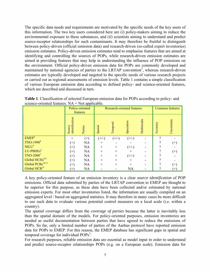
The specific data needs and requirements are motivated by the specific needs of the key users of this information. The two key users considered here are (i) policy-makers aiming to reduce the environmental exposure to these substances, and (ii) scientists aiming to understand and predict source-receptor relationships for such contaminants. It may therefore be fruitful to distinguish between policy-driven (official emission data) and research-driven (so-called expert inventories) emission estimates. Policy-driven emission estimates tend to emphasise features that are aimed at identifying and controlling the sources of POPs, while research-driven emission estimates are aimed at providing features that may help in understanding the influence of POP emissions on the environment. Official policy-driven emission data for POPs are commonly developed and maintained by national agencies of parties to the LRTAP convention3, whereas research-driven estimates are typically developed and targeted to the specific needs of various research projects or carried out as regional assessments of emission levels. Table 1 contains a simple classification of various European emission data according to defined policy- and science-oriented features, which are described and discussed in turn. Table 1. Classification of selected European emission data for POPs according to policy- and science-oriented features. NA = Not applicable.

Policy-oriented features

Research-oriented features Common features

Sour

ce

iden

tific

atio

n

Parti

es

Spat

ial

Tem

pora

l

Spec

iatio

n

Mul

timed

ia

Acc

urac

y

Unc

erta

inty

EMEP3 + (+) (+/-) (+/-) (+/-) - ? - TNO-19904 (+) NA + - - - ? (+) NILU5 (+) NA + + (+/-) - ? - LU-PBDEs6 (+) NA + + + - ? (+) TNO-20007 (+) NA + + (+/-) - ? - Global HCHs8,9 (+) NA + + + - ? - Global PCBs10,11 (+) NA + + + - ? (+) Global HCB12 (+) NA - - NA - ? (+) A key policy-oriented feature of an emission inventory is a clear source identification of POP emissions. Official data submitted by parties of the LRTAP convention to EMEP are thought to be superior for this purpose, as these data have been collected and/or estimated by national emission experts. For most other inventories listed, the information are usually compiled on an aggregated level / based on aggregated statistics. It may therefore in many cases be more difficult to use such data to evaluate various potential control measures on a local scale (i.e. within a country). The spatial coverage differs from the coverage of parties because the latter is inevitably less than the spatial domain of the models. For policy-oriented purposes, emission inventories are needed as useful documentation between parties that have agreed to reduce the emissions of POPs. So far, only a limited number of parties of the Aarhus protocol have reported emission data for POPs to EMEP. For this reason, the EMEP database has significant gaps in spatial and temporal coverage for individual POPs3. For research purposes, reliable emission data are essential as model input in order to understand and predict source-receptor relationships POPs (e.g. on a European scale). Emission data for

6

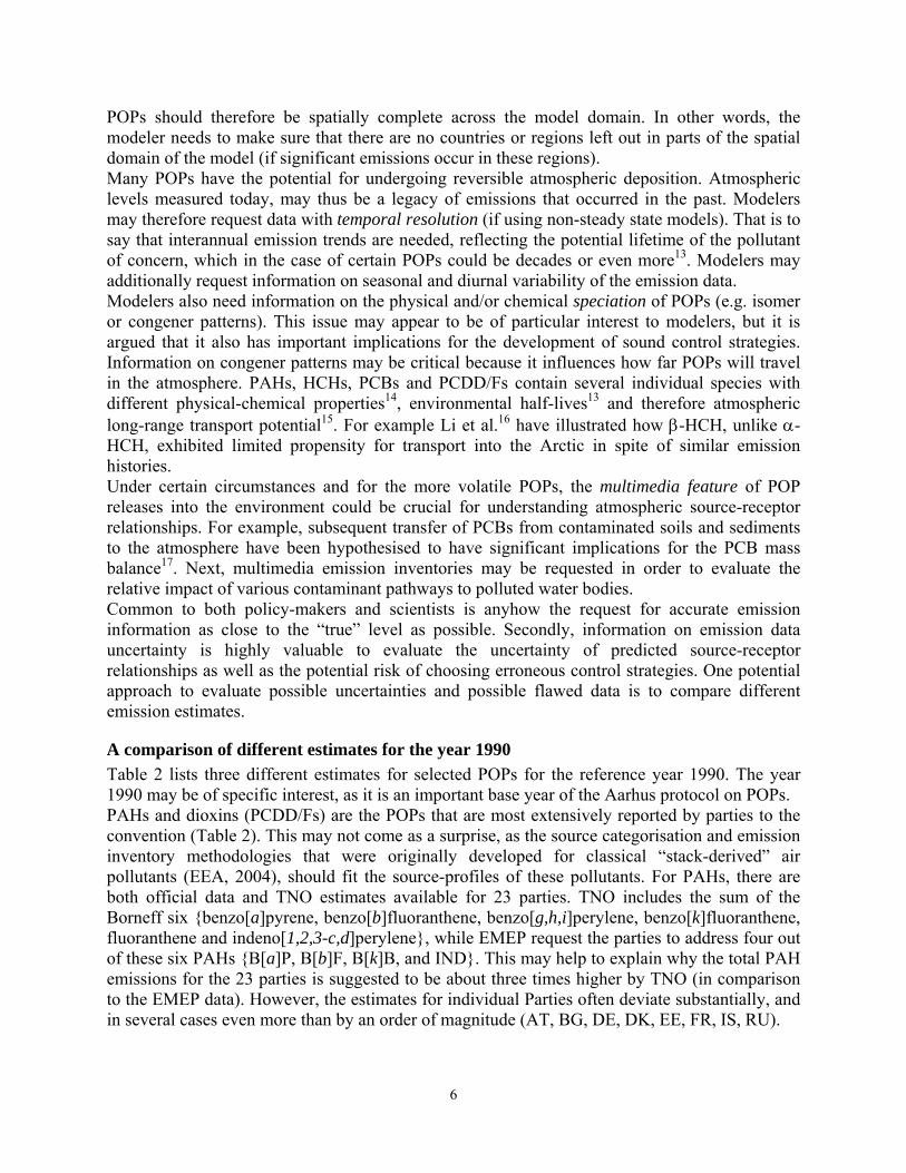
POPs should therefore be spatially complete across the model domain. In other words, the modeler needs to make sure that there are no countries or regions left out in parts of the spatial domain of the model (if significant emissions occur in these regions). Many POPs have the potential for undergoing reversible atmospheric deposition. Atmospheric levels measured today, may thus be a legacy of emissions that occurred in the past. Modelers may therefore request data with temporal resolution (if using non-steady state models). That is to say that interannual emission trends are needed, reflecting the potential lifetime of the pollutant of concern, which in the case of certain POPs could be decades or even more13. Modelers may additionally request information on seasonal and diurnal variability of the emission data. Modelers also need information on the physical and/or chemical speciation of POPs (e.g. isomer or congener patterns). This issue may appear to be of particular interest to modelers, but it is argued that it also has important implications for the development of sound control strategies. Information on congener patterns may be critical because it influences how far POPs will travel in the atmosphere. PAHs, HCHs, PCBs and PCDD/Fs contain several individual species with different physical-chemical properties14, environmental half-lives13 and therefore atmospheric long-range transport potential15. For example Li et al.16 have illustrated how β-HCH, unlike α-HCH, exhibited limited propensity for transport into the Arctic in spite of similar emission histories. Under certain circumstances and for the more volatile POPs, the multimedia feature of POP releases into the environment could be crucial for understanding atmospheric source-receptor relationships. For example, subsequent transfer of PCBs from contaminated soils and sediments to the atmosphere have been hypothesised to have significant implications for the PCB mass balance17. Next, multimedia emission inventories may be requested in order to evaluate the relative impact of various contaminant pathways to polluted water bodies. Common to both policy-makers and scientists is anyhow the request for accurate emission information as close to the “true” level as possible. Secondly, information on emission data uncertainty is highly valuable to evaluate the uncertainty of predicted source-receptor relationships as well as the potential risk of choosing erroneous control strategies. One potential approach to evaluate possible uncertainties and possible flawed data is to compare different emission estimates.

A comparison of different estimates for the year 1990 Table 2 lists three different estimates for selected POPs for the reference year 1990. The year 1990 may be of specific interest, as it is an important base year of the Aarhus protocol on POPs. PAHs and dioxins (PCDD/Fs) are the POPs that are most extensively reported by parties to the convention (Table 2). This may not come as a surprise, as the source categorisation and emission inventory methodologies that were originally developed for classical “stack-derived” air pollutants (EEA, 2004), should fit the source-profiles of these pollutants. For PAHs, there are both official data and TNO estimates available for 23 parties. TNO includes the sum of the Borneff six {benzo[a]pyrene, benzo[b]fluoranthene, benzo[g,h,i]perylene, benzo[k]fluoranthene, fluoranthene and indeno[1,2,3-c,d]perylene}, while EMEP request the parties to address four out of these six PAHs {B[a]P, B[b]F, B[k]B, and IND}. This may help to explain why the total PAH emissions for the 23 parties is suggested to be about three times higher by TNO (in comparison to the EMEP data). However, the estimates for individual Parties often deviate substantially, and in several cases even more than by an order of magnitude (AT, BG, DE, DK, EE, FR, IS, RU).

7

As an unintentional by-product of combustion, emissions of PCDD/Fs are also expected to take place in all countries. 26 parties report emissions higher than zero. For the total of emissions from these parties, the EMEP data shows the highest sum. Large discrepancies (more than 100%) between the official data and one or both independent estimates are evident for BG, CZ, DK, FI, HR, HU, IS, NO, SE, SK. The primary atmospheric emissions of PCBs may either be a result of (i) past intentional production, use and disposal of intentionally produced PCBs, or (ii) the unwanted formation of PCBs as a result of de-novo synthesis in various combustion processes11. Only 11 parties have submitted official emission data (greater than zero) for 1990. For the total emissions of PCBs from 11 parties, it can be seen that the EMEP estimates are about half of the TNO estimates. Table 2. Comparison of estimated national total emissions in 1990 (Units: PAHs in tonnes/year, PCDD/Fs in g I-TEQ/year; HCB and PCBs in kg/year)3.

PAHs PCBs HCB PCDD/Fs TNO EMEP TNO EMEP TNO NILU EMEP TNO EMEP NILU

AM NE X NE X NE NE X NE X NE AT 243.4 17.5 1319 NE 1 81 93 85 161 142 BA 47.8 X 128 X 20 NE X 9 X NE BE 818.0 199.4 5202 NE 213 73 18 616 624 520 BG 55.0 677.3 317 258 0 400 544 154 554 67 BY 191.0 X 600 X 0 570 X 106 X 107 CA NE 667.4 NE X NE NE 88.9 NE 436 NE CH 96.0 X 1644 X 4 59 0 242 242 242 CS 171.7 X 435 X 50 NE X 112 X NE CY 0.2 X 44 X 0 NE X 1 1 [5] NE CZ 259.2 751.6 1995 773 70 NE X 224 1252 216 DE[1] 419.8 0.7 42956 43579 86 1700 86 1196 1196 1623 DK 76.7 7.0 988 NA 103 130 NA 71 0 77 EE 28.3 0.3 179 X 0 87 X 18 X 15 ES 520.6 176.5 8536 0 1176 1200 6647 134 182 300 FI 104.4 15.8 2620 X 0 130 X 53 30 188 FR 3478.7 43.6 19520 88 11 1300 1649 1636 1765 1229 GB 1437.0 224.1 3453 7138 1240 550 3515 881 1232 974 GR 152.7 X 251 X 0 200 X 25 X 155 HR 54.0 15.1 132 X 30 NE 0.3 13 179 NE HU 192.4 132.0 129 135 4538 430 0.3 167 157 76 IE 73.7 X 62 X 0 47 X 44 X 17 IS 6.4 0.1 47 X 0 7 NE 0.6 10 0.2 IT 693.6 91.9 5825 X 406 840 X 583 443 873 LT 52.3 X 220 X 0 210 X 23 X 24 LU[2] 6.2 X 119 X 0 3 X 28 40 58 LV 38.4 X 162 X 0 160 X 14 X 13 MC NE <0.1 NE <1 NE NA X NE 2.4 NE MD 58.1 6.2 268 X 0 140 X 23 X 18 MK 21.7 X 82 X 0 NE X 4.9 X NE NL[3] 183.6 1707 251 0 0 93 0 505 743 373 NO 140.2 14.5 384 X 1 45 X 39 130 45 PL 372.0 159.2 2372 2425 0 1300 62 359 529 425 PT 137.7 X 523 X 0 160 X 17 X 40 RO 723.3 X 516 X 53 970 X 1500 X 129 RU 3146.0 18.3 10202 X 1 12000 1.6 1412 991 1849 SE[4] 282.0 38.8 1935 NE 3 160 NE 84 53 282 SI 50.5 23.5 71 357 0 NE 0 6.0 8.6 NE SK 310.0 41.9 1334 164 30 NE X 43 189 75 UA 1136.8 X 3736 X 0 2600 X 877 X 925 US NE 15642 NE 102 NE NE 1450 NE 234 NE Total 15779 20672 118557 55019 8036 25645 14156 11306 11378 11077 Count 37 26 37 11 19 29 13 37 26 31 For country codes see: www.emep.int/grid/country_numbers.txt X = No reporting, NA = Not Applicable, NE = Not Estimated, [1] Data for PAHs and PCBs refer to data for 1985-1990 submitted by the country, [2] 1993 data submitted by the country, [3] 1993 data submitted by the country, [4] 1987/1991 data submitted by the country, [5] EB.AIR/GE.1/2003/6.corr. For the data presented TNO, the following colour codes have been used: Black: data submitted by the country Red: data estimated by TNO, not approved by the country Black: subdivision of country (sub)total based on TNO estimates, not approved by the country Red: summation of country data and TNO data not approved by country

http://www.emep.int/grid/country_numbers.txt

8

Again, difference in compounds included within the group of PCBs is an issue that may help to explain deviations between these two estimates. The TNO estimates address total PCBs (i.e. the sum of 209 different compounds) when dealing with leakage or evaporation - or the sum of six frequently reported congeners (PCB-28, PCB-52, PCB-101, PCB-118, PCB-153 and PCB-180). For the official data, the actual composition of the PCB emissions referred to is not known. Hexachlorbenzene (HCB) has been used as a fungicide and is known as an impurity in other pesticides as well as a by-product from the production of chlorinated solvents. There may also be unintended formation and emissions of HCB from various industrial processes involving chlorine12. 13 parties report emissions of HCB in 1990 being greater than zero. The TNO estimate is a bit more than half of the sum of official data, whilst the NILU data is about 1.5 times the sum of official submissions. Again, there are substantial deviations between the official data and independent estimates by NILU and TNO. NILU suggests that the emissions in Russia were about three orders of magnitude higher than the data submitted to EMEP. NILU also suggests higher emissions than the other estimates for CH, DE, NL and PL, whilst TNO suggest higher emissions for HU as compared to the other inventories.

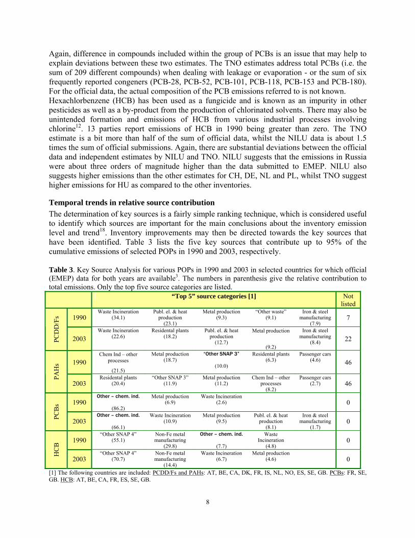
Temporal trends in relative source contribution The determination of key sources is a fairly simple ranking technique, which is considered useful to identify which sources are important for the main conclusions about the inventory emission level and trend18. Inventory improvements may then be directed towards the key sources that have been identified. Table 3 lists the five key sources that contribute up to 95% of the cumulative emissions of selected POPs in 1990 and 2003, respectively. Table 3. Key Source Analysis for various POPs in 1990 and 2003 in selected countries for which official (EMEP) data for both years are available3. The numbers in parenthesis give the relative contribution to total emissions. Only the top five source categories are listed.

“Top 5” source categories [1] Not listed

1990 Waste Incineration

(34.1) Publ. el. & heat

production (23.1)

Metal production (9.3)

“Other waste” (9.1)

Iron & steel manufacturing

(7.9) 7

PCD

D/F

s

2003 Waste Incineration

(22.6) Residental plants

(18.2) Publ. el. & heat

production (12.7)

Metal production

(9.2)


(8.4) 22

1990 Chem Ind – other

processes

(21.5)


“Other SNAP 3”

(10.0)

Residental plants (6.3)

Passenger cars (4.6) 46

PAH

s

2003 Residental plants

(20.4) “Other SNAP 3”

(11.9) Metal production

(11.2) Chem Ind – other

processes (8.2)

Passenger cars (2.7) 46

1990 Other – chem. ind.

(86.2)


Waste Incineration (2.6)

0

PCB

s

2003 Other – chem. ind.

(66.1)



Publ. el. & heat production

(8.1)


(1.7) 0

1990 “Other SNAP 4”

(55.1) Non-Fe metal manufacturing

(29.8)

Other – chem. ind.

(7.7)

Waste Incineration

(4.8)

0

HC

B

2003 “Other SNAP 4”

(70.7) Non-Fe metal manufacturing

(14.4)



0

[1] The following countries are included: PCDD/Fs and PAHs: AT, BE, CA, DK, FR, IS, NL, NO, ES, SE, GB. PCBs: FR, SE, GB. HCB: AT, BE, CA, FR, ES, SE, GB.

9

For simplicity, only the top 5 source categories are listed for those pollutants that have more than five source categories contributing to 95% of the total emissions. Please observe that the number of countries is limited. This is because we only included parties for which data in NFR (Nomenclature for Reporting) format3 are available. The years 1990 and 2003 were considered to evaluate potential temporal changes in the key sources. Waste incineration has been, and still is, recognised as the most important source category for emissions of PCDD/Fs19. As recognised for Belarus, it should also be recognised that waste incineration may not necessarily be the key source of dioxins for any country20. The relative importance of dioxin emissions from residential plants is also increasing in recent years (see also Lee et al.21). Still, there is a particular concern for PCDD/Fs if all relevant sources have been included in the inventory (i.e. completeness). It is therefore worth emphasising that a key source analysis does not consider the risk for incomplete coverage of the true key sources. The dioxin emissions from the open burning of household waste have received considerable attention22. However, reliable estimates of the relative importance of such emissions are considered difficult because of the lack of reliable activity data and emission factors related to open burning. For PAHs, various other processes in the chemical industries and metal production where the two key sources in 1990. At that time, other sources contributed 10%, or less. Nowadays, residential plants are suggested to be the key sources of PAHs. The result thus mirrors PCDD/Fs with respect to the relative increase in residential plant emissions from 1990 to 2003. For PCBs, only five source categories are addressed. Other processes in the chemical industries are attributed as the key source in both years. According to the explanatory notes from United Kingdom (which is one out of three parties reporting emissions of PCBs in NFR format), this source category accounts for emissions from capacitors, fragmentisers and transformers. As for the dioxins, there is a general concern if all true sources of PCBs are known11,21. Only a limited number of sources are also recognised for HCB. The key source is attributed to “Other” (includes agrochemical and pesticide use). The frequent assignment of POP emissions to “other” source categories as well as the limited number of sources listed, serve to illustrate that the official reporting scheme (originally developed for classical air pollutants) may be considered less suitable when applied to industrial chemicals and pesticides.

Closing remarks While strong efforts have been made to improve emission inventories needed for research on ozone depletion, climate change and acid deposition, inventories for POPs have for many years been considered unreliable and inaccurate23,24. A number of studies have highlighted that emission data are frequently the most uncertain input that determines the overall uncertainty of model predictions for POPs25-27. In fact, it has been claimed in several reviews that the emissions of POPs remains the least understood part of the overall distribution and fate of these chemicals in the environment25,28,29. Complete and accurate official emission data should anyhow be the preferred choice of emission information. This is because the national experts are expected to know the detailed characteristics in their respective countries concerning use of various pesticides, industrial chemicals and fuels, industrial processes and abatement technologies, which are controlling the emission levels of various toxic compounds. Furthermore, official emission data is the only emission information that seems suitable as documentation in international negotiations between parties that have agreed to reduce their emissions. Finally, official estimates also seem most

10

suitable when evaluating further emission reductions. In summary, official emission data are considered superior for the purpose of supporting decision-making processes at the national and international level. However, lack of information on spatial, temporal, speciation and multimedia features may obstruct the applicability for use by modelers. For this reason, modelers may still have to rely on research-driven estimates, which are typically targeted to meet the specific objectives of various individual research projects30. The overall goal of many research-driven estimates is typically a desire to present the “big picture” of emissions of individual POP substances in quantitative terms. We hope that future studies on emission inventories of POPs will recognise and address the emission inventory features that are needed for both scientific and regulatory purposes. Further development of official emission data with respect to the research-oriented features seems to be the way to proceed.

Acknowledgements

The EMEP programme is gratefully acknowledged for financial support.

References

1. The Stockholm Convention on Persistent Organic Pollutants. www.pops.int 2. The 1979 Geneva Convention on Long-Range Transboundary Air Pollution. www.unece.org/env 3. Vestreng V., Breivik K., Adams M., Wagner A., Goodwin J., Rozovskaya O. and Pacyna J.M. 2005.

Inventory Review 2005. Emission Data reported to LRTAP Convention and NEC Directive. Initial review for HMs and POPs. EMEP Technical Report MSC-W 1/2005. 114 pp. ISSN 0804-2446. see also webdab.emep.int

4. Berdowski J.J.M., Baas J., Bloos J.P.J., Visschedijk A.J.H. and Zandveld P.Y.J., 1997. The European Emission Inventory of Heavy Metals and Persistent Organic Pollutants. Umweltforschungsplan des Bundesministers für Umwelt, Naturschutz und Reaktorsicherheit. Luftreinhaltung. Forschungsbericht 104 02 672/03. TNO, Apeldoorn, The Netherlands.

5. Pacyna J.M., Breivik K., Münch J. and Fudala, J. (2003). Atmos. Environ. 37: S119-S131. 6. Prevedouros K., Jones K.C. and Sweetman A.J. (2004) Environ. Sci. Technol. 38: 3224-3221. 7. Denier van der Gon H.A.C., van het Bolscher M., Visschedijk A.J.H. and Zandveld, P.Y.J. (2005).

Study to the effectiveness of the UNECE Persistent Organic Pollutants Protocol and cost of possible additional measures. Phase 1. Estimation of emission reduction results from the implementation of the POP Protocol. TNO-report B&O-A R 2005/194. TNO, Apeldoorn, The Netherlands.

8. Li Y.-F., Scholtz M.T. and van Heyst B.J. (2000). J. Geophys. Res. 105 (D5): 6621-6632. 9. Li Y.-F., Scholtz M.T. and van Heyst B.J. (2003). Environ. Sci. Technol. 37: 3493-3498. 10. Breivik K., Sweetman A., Pacyna J.M. and Jones, K.C. (2002). Sci. Total. Environ. 290: 181-198. 11. Breivik K., Sweetman A., Pacyna J.M. and Jones, K.C. (2002). Sci. Total. Environ. 290: 199-224. 12. Bailey R.E. (2001). Chemosphere 43: 167-182. 13. Sinkkonen S. and Paasivirta, J. (2000). Chemosphere 40: 943-949. 14. Mackay D., Shiu W.-Y. and Ma K.-C. 1999. Physical-chemical properties and environmental fate

handbook. Chapman&Hall / CRCnetBASE. CD-rom. ISBN 0-8493-9757-X. 15. Beyer A., Mackay D., Matthies M., Wania F. and Webster E. (2000). Environ. Sci. Technol. 34: 699-

703. 16. Li Y.-F., Macdonald R.W., Jantunen L.M.M., Harner T., Bidleman T.F., Strachan W.M.J. (2002) Sci.

Total. Environ. 291: 229-246. 17. Chiranzelli J.R., Scrudato R.J. and Wunderlich M.L. (1997) Environ. Sci. Technol. 30: 1797-1804.

http://www.pops.int/

http://www.unece.org/env

11

18. Rypdal K. and Flugsrud, K. (2001). Environ. Sci. Policy 4: 117-135. 19. McKay G. (2002). Chem. Eng. J. 86: 343-368. 20. Kakareka S.V. (2002). Atmos. Environ. 36: 1407-1419. 21. Lee R.G.M., Coleman P., Jones J.L., Jones K.C. and Lohmann R. (2005). Environ. Sci. Technol. 39:

1436-1447. 22. Lemieux P.M., Lutes C.C., Abbott J.A., Aldous K.M. (2000). Environ. Sci. Technol. 34: 377-384. 23. Graedel T.E., Bates T.S., Bouwman A.F., Cunnold D., Dignon J., Fung I., Jacob D.J., Lamb B.K.,

Logan J.A., Marland G., Middleton P., Pacyna J.M., Placet M. and Veldt C. (1993) Global Biogeochem. Cycles 7: 1-26.

24. Pacyna J.M. and Graedel T.E. (1995). Ann. Rev. Energy Environ. 20: 265-300. 25. Vallack H.W., Bakker D.J., Brand I., Broström-Lunden E., Brouwer A., Bull K.R., Gough C.,

Guardans R., Holoubek I., Jansson B., Koch R., Kuylenstierna J., Lecloux A., Mackay D., McCutcheon P., Mocarelli P. and Taalman R.D.F. (1998) Environ. Toxicol. Pharmacol. 6: 143-175.

26. Cohen M.D., Draxler R.R., Artz R., Commoner B., Bartlett P., Cooney P., Couchot K., Dickar A., Eisl H., Hill C., Quigley J., Rosenthal J.E., Niemi D., Ratte D., Deslauriers M., Laurin, M., Mathewson-Brake L. and McDonald J. (2002). Environ. Sci. Technol. 36: 4831-4845.

27. Malanichev A., Mantseva E., Shatalov V., Strukov B. and Vulykh N. (2004). Environ. Pollut. 128, 279-289.

28. Wania F. and Mackay D. (1996) Environ. Sci. Technol. 30: 390A-396A. 29. Jones K.C. and de Voogt P. (1999). Environ. Pollut. 100: 209-221. Breivik K., Alcock R., Li Y.-F., Bailey R.E., Fiedler H. and Pacyna J.M. (2004). Environ. Pollut. 128: 3-1

12

CONTEMPORARY SOURCES OF DDTs IN NORTH AMERICAN AIR

Terry F. Bidleman1, Fiona Wong2, Henry A. Alegria3, Perihan Kurt-Karakus4, Kevin C. Jones4

1. Centre for Atmospheric Research Experiments, Environment Canada, 6248 Eighth Line, Egbert, ON, L0L 1N0, Canada

2. Environment Canada, 4905 Dufferin St., Downsview, ON, M3H 5T4, Canada 3. Chemistry Department, California Lutheran University, Thousand Oaks, CA, 91360, U.S.A.

4. Environmental Science Department, Lancaster University, Lancaster, LA1 4YQ, UK

Introduction DDT is among the 12 persistent organic pollutants (POPs) to be eliminated worldwide under the Stockholm Convention (UNEP, 2001). However, due to threats from malaria and other vector-borne diseases, DDT is still used in many tropical and subtropical regions. DDT use for vector disease control is permitted under the Stockholm Convention in accordance with World Health Organization (WHO) guidelines. The position of WHO is that there will be a continued role for DDT in combating malaria, and that restrictions on DDT use for public health purposes should be accompanied by technical and financial measures to ensure that malaria control is maintained by alternative methods. Although DDT has been deregistered in Canada and the U.S. for decades, residues are still found in soil, air and precipitation. An open question is whether the DDTs found in atmospheric samples are due to long-range transport from countries where DDT is currently used, emissions from "legacy" residues in soils or both. The issue was raised 20 years ago in a classic paper by Robert Rapaport and coworkers, "New" DDT in North America -- Atmospheric Deposition1. The authors analysed cores from peat bogs collected in the Great Lakes region and eastern Canada for DDT residues to determine historical loadings and modern deposition in the early 1980s. They noted that, while total DDT residues (ΣDDT) peaked in the mid- to late-1960s, deposition in the late 1970s and early 1980s continued at a lower level and declined more slowly. Moreover, the composition of ΣDDT in recent peat layers was marked by a high proportion of "fresh" DDT (p,p'-DDT and o,p'-DDT) in comparison to stable DDT degradation products (DDDs and DDEs). These observations led the authors to suggest that DDT was undergoing air transport from Mexico and Central America, nearly a decade after its 1972 deregistration in the United States. Contemporary levels of ΣDDT in the atmosphere of southern Mexico exceed average ambient air concentrations in the U.S. and Canada by an order of magnitude or more2-4. These measurements were made between 2000-2004, coincident and just after Mexico officially stopped using DDT for vector control. Some portion of this DDT may be influencing air concentrations in other parts of the continent, but there are other potential sources of DDT and other chlorinated pesticides to be considered: air transport across the Pacific Ocean from Asia5,6 and emission of soil residues from past usage in the U.S. and Canada7-12. The availability of air data from Mexico, where DDT has been recently used, provides an opportunity for comparisons with the U.S. and Canada. Objectives of the study are to: a) set bounds on proportions of DDT residues that are expected from emission of legacy residues, b)

13

compare these limits with the proportions found in ambient air to determine if "new" DDT is present.

Experimental Sampling and analysis of DDT and other organochlorine pesticides in the ambient air of southern Mexico were carried out as described2,3. Briefly, air samples were collected with a glass fiber filter - polyurethane foam (GFF-PUF) cartridge. After extraction and cleanup, the pesticides were determined by capillary GC - electron capture negative ion mass spectrometry, using isotopically labeled pesticides as recovery surrogates.

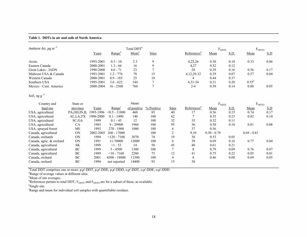
Levels of DDTs in the ambient air and soil of the U.S. and Canada were obtained from literature reports (Table 1). Some air data were from long-term surveys involving regular high volume air sampling over one or more years, or deployment of passive air samplers to integrate air concentrations over a full year. Other data were from short-term campaigns using active or passive samplers. Soil residue data collected since 1985 were from agricultural fields in British Columbia and Saskatchewan, Canada, California and the southern and midwestern U.S. states, Canadian orchards in British Columbia and Ontario, and forests in Maine which had been sprayed with DDT in the past.

Comparisons of DDT compound profiles in soil and overlying air were made at multiple sites in British Columbia8, the southern U.S.A.7 and at one Ontario farm9 by collecting air samples in close proximity to the soil (5-40 cm), using a GFF to exclude soil dust followed by a PUF plug to trap vapour-phase compounds. Fractionation of the DDTs between soil and air was predicted by assuming that compound volatility is directly related to the liquid-phase vapour pressure (VP) and inversely related to the octanol-air partition coefficient (KOA), e.g.

(p,p'-DDT/p,p'-DDE)air = (p,p'-DDT/p,p'-DDE)soil x VPDDT/VPDDE (1)

(p,p'-DDT/p,p'-DDE)air = (p,p'-DDT/p,p'-DDE)soil x KOA,DDE/KOA,DDT (2)

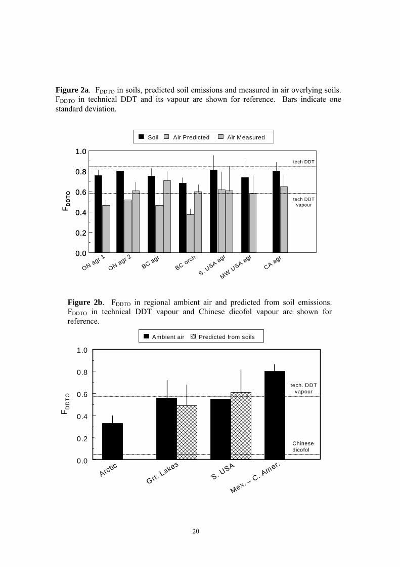
and similar relationships for p,p'-DDT/o,p'-DDT. VP and KOA values as functions of temperature were taken from Hinckley et al.13 and Shoeib and Harner14. DDT proportions were expressed as fractional values, FDDTE = p,p'-DDT/(p,p'-DDT + p,p'-DDE) and FDDTO = p,p'-DDT/(p,p'-DDT + o,p'-DDT), since fractions are preferred to ratios for statistical purposes15. Fractions = 0.5 corresponds to ratios = 1. The means and standard deviations in Figures 1 and 2 refer to the regional distributions of site-averaged FDDT, not to individual samples.

Results and Discussion Chemical markers for source identification

As mentioned above, DDT is degraded in soils to the stable products DDE and DDD. The ratio of p,p'-DDT/p,p'-DDE is often used as a rough gauge of residue age; a high ratio implies inputs from current use of DDT while a low ratio suggests old residues1. There are no generally accepted limits for "high" and "low" ratios and how these related to "new" and "old" DDT.

Another potential source of DDT residues is the pesticide dicofol, which is manufactured from DDT. The dicofol made in China is contaminated with DDT residues that are especially high in o,p'-DDT and the p,p'-DDT/o,p'-DDT ratio is useful for identifying "dicofol-type" DDT contamination16.

14

The two enantiomers of o,p'-DDT are often degraded in soil at different rates and volatilization of nonracemic o,p'-DDT is a tracer of soil emissions. A problem is that o,p'-DDT degradation in soils is ambivalent; residues in soil show preferential degradation of the (+) enantiomer, the (–) enantiomer or neither (racemic residues) with about equal frequency. This is the case in agricultural soils7,12,17,18, and also in background soils collected in a global survey19. Nonracemic o,p'-DDT has been used to trace emissions at specific fields7,12, and it has been noted that o,p'-DDT residues in ambient air from the Great Lakes region showed greater deviation from racemicity than air samples from the southern U.S.A. and Mexico4.

Proportions of DDT compounds

Figure 1a shows FDDTE and FDDTO in soils from the regions in Table 1 and the predicted fractions in air due to soil emissions. The fractionation relationships (eq 1) and (eq 2) were tested at experimental sites in the southern U.S.A., British Columbia and Ontario by collecting paired soil and air samples, as described above. FDDTE in the overlying air was accurately predicted by relative VP (eq 1) but greatly overestimated using the KOA relationship (eq 2). The average predicted/measured FDDTE was 1.00 ± 0.42 (eq 1) compared to 2.91 ± 1.78 (eq 2). The disparity was less for FDDTO, predicted/measured was 0.82 ± 0.16 (eq 1) and 1.00 ± 0.16 (eq 2).

p,p'-DDT and p,p'-DDE

Regional averages of FDDTE in soils of Canada and the U.S.A. ranged from 0.32 − 0.79 , and the predicted regional averages of FDDTE in air from soil emissions (eq 1) ranged from 0.07 − 0.36 (Table 1, Figure 1a). The overall average FDDTE in soil emissions from all regions averaged 0.19 ± 0.10. Regional averages of FDDTE in ambient air of the U.S.A. and Canada (including the Arctic) varied from 0.29 − 0.44 (Figure 1b), and the overall average of 0.32 ± 0.19 was higher than predicted from soil emissions. This might signify "new" DDT input from long-range transport, e.g. from Mexico - Central America where the mean FDDTE in ambient air was 0.59 ± 0.14 (Table 1, Figure 1b). On the other hand, the available soil residue data is rather sparse, and it is possible that there are emissions from soils which have not been included in the literature survey in Table 1. FDDTE in soils varies greatly due to soil management practices and microbial activity, which is responsible for DDT metabolism11,20,21. For example, some soils in the southwestern U.S.A. have an unusually high proportion of p,p'-DDT, which has been explained by lack of microbial activity21. These are not included in Table 1 because the authors only reported "DDT" and "DDE" and not the individual p,p'- and o,p'-species.

The Integrated Atmospheric Deposition Network, operated jointly by Environment Canada and the U.S. Environmental Protection Agency, is an especially rich source of air data for the DDTs. FDDTE was correlated to total DDT concentrations in air samples collected by the U.S. network at five Great Lakes sites from 1990-2000. The regression for 1119 points showed a significant correlation (p = 0.0035), but the r2 value was only 0.0076, indicating that the relationship explained less than 1% of the total variance. A similar analysis of 512 data points from two Canadian Great Lakes stations showed no significant correlation (p = 0.33). Thus, it is not likely that high concentrations of total DDT in Great Lakes air can be explained by transport of recently used DDT.

Considering transport across the Pacific, the FDDTE in air samples collected at Taihu Lake, China22 ranged from 0.24 − 0.52. FDDTE values calculated from air concentrations measured at Tagish, Yukon, Canada in 1993-94 averaged 0.06 when air transport was from India and 0.16 when transport was from eastern Asia5. Transport events from western North America resulted

15

in lower air concentrations, but higher FDDTE ranging from 0.11 − 0.21 in winter and 0.57 - 0.74 in summer5.

p,p'-DDT and o,p'-DDT

The database for o,p'-DDT is smaller than for p,p'-DDE. FDDTO in soils ranged from 0.69 - 0.81 and averaged 0.76 ± 0.05 (Table 1, Figure 2a). FDDTO = 0.84 in technical DDT, using the "typical" composition 77.1% p,p'-DDT, 14.9% o,p'-DDT, 4% p,p'-DDT given by World Health Organization (WHO)23. FDDTO in predicted soil emissions (eq 1) ranged from 0.38 - 0.61 (mean = 0.51 ± 08) (Figure 2a). The expected FDDTO in technical DDT vapour is 0.58. Similar FDDTO values were found in ambient air of the Great Lakes - midwestern U.S.A. and the southern U.S.A. (0.55 - 0.57, Table 1, Figure 2b). The proximity of ambient air to technical DDT vapour is probably not the result of current DDT usage, but rather because FDDTO values in soils are rather similar to the technical DDT composition. FDDTO in ambient air of Mexico - Central America is 0.80 ± 0.05 (Table 1, Figure 2b). This is much higher than in technical DDT vapour, and cannot be explained by vapourization of technical DDT having the WHO composition. Other technical DDT compositional information summarized by Metcalf24 show widely varying percentages of p,p'-DDT (48-80%) and o,p'-DDT (11-29%). Improved information on the composition of DDT products used in Canada, the U.S.A. and Mexico would be helpful.

The question of possible "dicofol-type" DDT contamination can be addressed by examining FDDTO. The average percentages of the two DDT isomers in Chinese dicofol products are 1.7% p,p'-DDT and 11.4% o,p'-DDT16. This results in FDDTO = 0.13 for dicofol and a predicted FDDTO = 0.04 for the vapour (eq 1). The much higher FDDTO values in ambient air, similar to predicted soil emissions (Figure 2b), virtually rules out contributions of "dicofol type" DDT to ambient air in the southern U.S.A. and Great Lakes region. This is reasonable, since the dicofol sold in Canada and the U.S.A. must have less than 0.1% DDT residues. The o,p'-DDT isomer has not been reported in air samples from western Canada, so the possibility of transpacific transport cannot be assessed at this time. Summary and the Path Forward The above assessment indicates that emission of legacy residues in Canadian and U.S.A. soils can support FDDTE = 0.19 ± 0.10 in air. Until better information is available, it is suggested that this result can be used as a guideline against which to judge possible new DDT inputs. Ambient air samples from most regions of Canada and the U.S.A. show higher FDDTE = 0.32 ± 0.19, which might indicate contributions other than soil emissions. FDDTE = 0.59 ± 0.14 in the air of southern Mexico - Central America, and the residue composition at some sites suggests fresh DDT usage. Examination of FDDTO values suggests no contribution of "dicofol-type" DDT contamination to the southern U.S.A. and the Great Lakes.

These conclusions are tentative, and depend greatly on the accuracy of the soil emission predictions. The latter are limited by lack of representative soil residue data which cover the regions of interest, and a rudimentary understanding of the soil-air exchange process. DDT residues in North American soils vary by several orders of magnitude (Table 1), and while FDDTE and FDDTO are far less variable, soils with high residues are likely to control atmospheric concentrations and DDT compound proportions. Regarding soil-air exchange, it is unknown why FDDTE predictions using KOA are less accurate than with VP, whereas FDDTO is reasonably well predicted using either property. Emission predictions using KOA or VP alone do not account

16

for the variability in types of soil organic matter. Aging of pesticides in soil reduces their bioavailability42,43, but it is not known if the same sequestering process by soils also limits volatilisation.

Steps toward a better understanding of DDT sources in North America are to: a) Obtain air concentration data from Mexico across the entire country. Current campaigns cover only the southern region. b) Collect regionally representative soil residue data in Canada, the U.S.A. and Mexico, and c) Improve understanding of the soil-air exchange process. References 1. Rapaport, R., Urban, N., Capel, P., Baker, J., Looney, B., Eisenreich, S., Gorham, E. (1985).

Chemosphere 14: 1167-1173.

2. Alegria, H., Bidleman, T., Salvador Figueroa, M. (2005). Environ. Pollut., in press.

3. Alegria, H., Wong, F., Bidleman, T., Salvador Figueroa, M., Gold Bouchot, G., Waliszewski, S., Ceja Moreno, V., Infanzon, R. (2005). In: Vazquez Botello, A., Rendón von Osten, J., Agraz Hernández. C., Gold Bouchot, G., eds . Golfo de México, Contaminación e Impacto Ambiental: Diagnóstico y Tendencia, Universidad Autónoma de Campeche, Mexico, in press.

4. Shen, L., Wania, F., Lei, Y., Teixeira, C., Muir, D., Bidleman, T. (2005). Environ. Sci. Technol. 39: 409-420.

5. Bailey, R., Barrie, L., Halsall, C., Fellin, P., Muir, D. (2000). J. Geophys. Res. 105: 11805-11811.

6. Killin, R., Simonich, S., Jaffe, D., DeForest, C., Wilson, G. (2004). J. Geophys. Res. 109: D23S15.

7. Bidleman, T., Leone, A. (2004). Environ. Pollut. 128: 49-57

8. Bidleman, T., Leone, A., Wong, F., Van Vliet, L., Szeto, S., Ripley, B. (2005). Environ. Toxicol. Chem., submitted.

9. Kurt-Karakus, P., Bidleman, T., Staebler, R., Jones, K. (2005). in preparation.

10. Meijer, S., Shoeib, M., Jantunen, L., Jones, K., Harner, T. (2003). Environ. Sci. Technol. 33: 1292-1299.

11. Spencer, W., Singh, G., Taylor, C., LeMert, R., Cliath, M., Farmer, W. (1996). J. Environ. Qual. 25: 815-821.

12. Leone, A., Amato, S., Falconer, R. (2001). Environ. Sci. Technol. 35: 4592-4596.

13. Hinckley, D., Bidleman, T., Foreman, W., Tuschall, J. (1990). J. Chem. Eng. Data 35: 232-237.

14. Shoeib, M., Harner, T. (2002). Environ. Toxicol. Chem. 21: 984-990.

15. Ulrich, E., Helsel, D., Foreman, W. (2003). Chemosphere 53: 531-538.

16. Qiu, X., Zhu, T., Yao, B., Hu, J., Hu, S. (2005). Environ. Sci. Technol. 39: 4385-4390.

17. Aigner, E., Leone, A., Falconer, R. (1998). Environ. Sci. Technol. 32: 1162-1168.

18. Wiberg, K., Harner, T., Wideman, J., Bidleman, T. (2001). Chemosphere 45: 843-848.

19. Kurt-Karakus, P., Bidleman, T., Jones, K. (2005). Environ. Sci. Technol., in press.

20. Boul, H., Garnham, M., Hucker, D., Baird, D., Alsiable, J. (1994). Environ. Sci. Technol. 28: 1397-1402.

21. Hitch, R., Day, H. (1992). Bull. Environ. Contam. Toxicol. 48: 259-264.

17

22. Qiu, X., Zhu, T., Li, J., Pan, H., Li, Q., Miao, G., Gong, J. (2004). Environ. Sci. Technol. 38: 1368-1374.

23. World Health Organization (1989). Environmental Health Criteria for DDT and its Derivatives, Environmental Aspects. ISBN 92-4-154283-7. World Health Organization, Geneva, Switzerland.

24. Metcalf, R. (1955). Organic Insecticides, Their Chemistry and Mode of Action. Interscience Publishers, NY.

25. Hung, H., Halsall, C., Blanchard, P., Li, H., Fellin, P., Stern G., Rosenberg, B. (2002). Environ. Sci. Technol. 36: 862-868.

26. Hung, H., Blanchard, P., Halsall, C., Bidleman, T., Stern, G., Fellin, P., Muir, D., Barrie, L., Jantunen, L., Helm, P., Ma, J., Konoplev, A. (2005). Temporal and spatial variabilities of atmospheric POPs in the Canadian Arctic: results from a decade of monitoring. Sci. Total Environ. 342: 119-144.

27. Aulagnier, F., Poissant, L. (2005). Environ. Sci. Technol. 39: 2960-2967.

28. Integrated Atmospheric Deposition Network (IADN) data base, Environment Canada.

29. Harner, T., Shoeib, M., Diamond, M., Stern, G., Rosenberg, G. (2004). Environ. Sci. Technol. 38: 4474-4483.

30. Motelay-Massei, A., Harner, T., Shoeib, M., Diamond, M., Stern, G., Rosenberg, B. (2005). Environ. Sci. Technol. 39: 5763-5773.

31. Hoh, E., Hites, R.A. (2004). Environ. Sci. Technol.38: 4187-4194.

32. Coupe, R., Manning, M., Foreman, W., Goolsby, D., Majewski, M. (2000). Sci. Tot. Environ. 248: 227-240.

33. Jantunen, L., Bidleman, T., Harner, T., Parkhurst, W. (2000). Environ. Sci. Technol. 34: 5097-5105.

34. Park, J-S., Wade, T., Sweet, S. (2001). Atmos. Environ. 35: 3315-3324.

35. Kannan, K., Battula, S., Loganathan, B., Hong, C-S., Lam, W., Villeneuve, D., Sajwan, K., Giesy, J., Aldous, K. (2003). Arch. Environ. Contam. Toxicol. 45: 30-36.

36. Mischke, T., Brunetti, K., Acosta, V., Weaver, D., Brown, M. (1985). Agricultural Sources of DDT Residues in California's Environment. California Department of Food and Agriculture, Sacramento, CA.

37. Dimond, J., Owen, R. (1996). Environ. Pollut. 92: 227-230.

38. Harris, M., Wilson, L., Elliot, J., Bishop, C., Tomlin, A., Henning, K. (2000). Arch. Environ. Contam. Toxicol. 39: 205-220.

39. Webber, M., Wang, C. (1995). Can. J. Soil Sci. 75: 513-524.

40. Bailey, P., Waite, D., Quinnette-Abbott, L., Ripley, B. (2004). Can. J. Soil Sci. 85: 265-271

41. Szeto, S., Price, P. (1991). J. Agric. Food Chem. 39: 1679-1684.

42. Alexander, M. (2000). Environ. Sci. Technol. 34: 4259-4265.

43. Gevao, B., Jones, K., Semple, K., Craven, A., Burauel, P. (2003). Environ. Sci. Technol. 37: 138A-144A.

18

Ambient Air, pg m -3

Years Rangeb Meanc Sites Referencesd Mean S.D. Mean S.D

Arctic 1993-2001 0.3 - 10 3.3 9 4,25,26 0.30 0.10 0.33 0.06Eastern Canada 2000-2001 1.3 - 66 16 9 4,27 0.32 0.12Great Lakes - IADN 1990-2000 4.6 - 71 23 7 28 0.29 0.16 0.56 0.17Midwest USA & Canada 1993-2001 1.2 - 776 78 15 4,12,29-32 0.29 0.07 0.57 0.04Western Canada 2000-2001 0.9 - 185 25 10 4 0.44 0.37Southern USA 1995-2001 3.6 - 622 144 7 4,31-34 0.31 0.20 0.55e

Mexico - Cent. America 2000-2004 16 - 2300 760 7 2-4 0.59 0.14 0.80 0.05

Soil, ng g -1

Country and State or Meanf

land use province Years Rangef of positive % Positive Sites Referencesd Mean S.D. Mean S.DUSA, agricultural PA,OH,IN,IL 1995-1996 <0.5 - 11800 460 85 40 17 0.56 0.15 0.74 0.17USA, agricultural AL,LA,TX 1996-2000 0.1 - 1490 140 100 62 7 0.35 0.23 0.82 0.14USA, agricultural SC,GA 1999 0.1 - 45 12 100 32 35 0.32 0.11USA, agricultural CA 1985 8 - 29900 1960 100 95 36 0.50 0.18 0.81 0.08USA, sprayed forest ME 1993 270 - 1900 1000 100 6 37 0.56Canada, agricultural ON 2002-2005 260 - 17000 100 2 9,10 0.50 - 0.79 0.69 - 0.81Canada, orchards ON 1994 <120 - 7100 3070 74 19 38 0.53 0.05Canada, agric. & orchard ON 1991 11-70000 12000 100 6 39 0.69 0.16 0.77 0.04Canada, agricultural SK 1999 <1 - 53 14 50 45 40 0.61 0.21Canada, agricultural BC 1999 5 - 4500 1300 100 7 8 0.79 0.09 0.76 0.07Canada, agricultural BC 1989 <10 - 7160 2280 75 12 41 0.75 0.22 0.85 0.01Canada, orchard BC 2001 4300 - 18000 11300 100 4 8 0.46 0.08 0.69 0.05Canada, orchard BC 1994 not reported 14400 93 15 38

aTotal DDT comprises one or more: p,p'-DDT, p,p'-DDE, p,p'-DDD, o,p'-DDT, o,p'-DDE, o,p'-DDDbRange of average values at different sites.cMean of site averages.dReferences pertain to total DDT; FDDTE and FDDTO are for a subset of these, as available.eSingle site.fRange and mean for individual soil samples with quantifiable residues.

Table 1. DDTs in air and soils of North America

Total DDTa

FDDTE FDDTO

FDDTE FDDTO

19

F D

DTE

Arctic

E. Canada

Grt. Lake

s

W. Canada

S. USA

Average

Mex - C. A

mer.0.0

0.2

0.4

0.6

0.8

Ambient air Predicted from soils

tech. DDTvapour

F DD

TE

Arctic

E. Canada

Grt. Lake

s

W. Canada

S. USA

Average

Mex - C. A

mer.0.0

0.2

0.4

0.6

0.8


tech. DDTvapour

Figure 1a. FDDTE in soils, predicted soil emissions and measured in air overlying soils. FDDTE in technical DDT and its vapour are shown for reference. Bars indicate one standard deviation

Figure 1b. FDDTE in regional ambient air and predicted from soil emissions.

ON agr 2

ON orchSK ag

r

S. USA ag

r 1MW U

SA agr

Soil Air Predicted Air Measured

BC agr

BC orch

1BC or

ch 2

ME fores

tS. U

SA agr 2

CA agr

tech.DDT vapour

0.0

0.2

0.4

0.6

0.8

1.0

F DD

TE

0.0

0.2

0.4

0.6

0.8

1.0

F DD

TE

tech.DDT

ON agr 1

20

Figure 2a. FDDTO in soils, predicted soil emissions and measured in air overlying soils. FDDTO in technical DDT and its vapour are shown for reference. Bars indicate one standard deviation.

Figure 2b. FDDTO in regional ambient air and predicted from soil emissions. FDDTO in technical DDT vapour and Chinese dicofol vapour are shown for reference.

Arctic0.0

0.2

0.4

0.6

0.8

1.0


Grt. Lakes

S. USA

Mex. – C. Amer.

F DD

TO

tech. DDTvapour

Chinesedicofol

ON agr 2BC agr

S. USA agr

MW USA agr

CA agr

Soil Air Predicted Air Measured

BC orch0.0

0.2

0.4

0.6

0.8

1.0

F DD

TO

0.0

0.2

0.4

0.6

0.8

1.0

F DD

TO

tech DDT

tech DDTvapour

ON agr 1

21

ORGANIC COMPOUND-SPECIFIC TRACERS OF AEROSOL SOURCES AND TROPOSPHERIC REACTIONS

Joel E. Baker and Bernard S. Crimmins

University of Maryland Chesapeake Biological Laboratory, P.O. Box 38, 1 Williams

Street, Solomons, Maryland USA 20688 Introduction Transport and deposition of a wide range of chemical contaminants impact coastal water quality throughout the world. In our work, we have quantified atmospheric depositional loadings of persistent organic pollutants (PCBs, PAHs, and pesticides), metals, mercury, and the nutrient nitrogen to the Chesapeake Bay estuary. During the past decade, environmental agencies in the United States have started to include atmospheric deposition loadings into water quality regulations, recognizing the linkage between chemicals emitted to the atmosphere and subsequent water quality impacts. For several classes of highly bioaccumulative POPs, such as PCBs, atmospheric depositional loads alone are large enough to impair U.S. coastal waters. Managing this issue requires both quantifying the magnitude and relative importance of atmospheric deposition as well as determining the sources of these atmospheric contaminants. Sources include both the classical point (power generation, waste incineration, domestic heating) and non-point (transportation) sources, but also consideration of those POPs produced through secondary reactions in the atmosphere. The purpose of this paper is to review the tools available to estimate the sources of persistent organic pollutants in urban, rural, and global atmospheres. These techniques include compound-specific tracers and multivariate statistical techniques. Examples of each from our recent work in North America and the Indian Ocean are presented. Materials and Methods 1. Improving analytical sensitivity for enhanced temporal resolution. The most common analytical tool to quantify and identify organics in the atmosphere is gas chromatography/mass spectrometry (GC/MS). Sample extracts are generally concentrated to >100 L and only 2 L or less of that extract is applied to the column using conventional inlets (hot splitless and cool on-column). For semi-volatile compounds (i.e. PAHs and nitro-PAHs) concentrating extracts below this volume may increase losses of the more volatile components. Therefore 98% of the analyte mass extracted is not introduced into the chromatographic system. With the advent of large volume injection techniques, the widely used hot splitless injection technique can be modified to load a greater portion of an extract (from 2 L to 100s of L). The commercial availability of Programmed Temperature Vaporization (PTV, Gerstel) inlet has made this injector attractive for trace level analysis. Other large volume techniques, such as cool on-column injection with solvent vent (SVE-COC) may be quickly degraded by system fouling from complex sample extracts (see Grob and Biedermann1 for review). Like the splitless injector, the PTV incorporates a glass sleeve that traps nonvolatile contaminants, keeping them from degrading the capillary column. Enhanced temporal resolution of air toxics such as PAHs and NPAHs is critical to understanding their sources and behavior in the ambient atmosphere. We present a large volume injection technique for the quantification of both classes of compounds2. The programmed temperature vaporization large-volume injection techniques has similar

22

precision as the standard hot splitless injection, while enhancing the sensitivity per mass injected up to 5-fold for PAHs. The methods were verified using microgram quantities of Standard Reference Materials. 2. Use of compound-specific tracers of primary and secondary aerosols. Nitro-substituted polycyclic aromatic hydrocarbons (NPAHs) are of concern in the urban atmosphere due to their direct mutagenic properties. This class of contaminants has primary and secondary sources with specific isomeric compositions3. Numerous chamber studies have elucidated the formation products and mechanisms of secondary NPAHs under a variety of conditions. During the Baltimore PM.2.5 Supersite intensives (spring summer and winter 2002-2003), bulk and size-resolved aerosol was collected and analyzed for NPAHs and parent polycyclic aromatic hydrocarbons (PAHs), hopanes and n-alkanes. Co-located measurements of elemental and organic carbon as well as NOx, O3 and PM2.5 were also performed. Six hour integrated bulk aerosol and 12 and 24 hr size resolved PAH and NPAH measurements are employed to assess the dominant sources of primary and secondary NPAHs to the Baltimore atmosphere. As an additional demonstration, the PAH composition of ambient aerosols collected over the Indian Ocean were determined during the INDOEX campaigns4. Use of the sensitive PTV-based analytical techniques described below allowed accurate quantification of PAHs at very low levels on relatively small samples. Here we explored the ratios of individual PAHs to elemental and organic carbon as tracers of combustion sources. The specific objective was to determine the relative importance of biomass and fossil fuel combustion as aerosols sources in the northern Indian Ocean atmosphere. 3. Application of multivariate statistical techniques. Understanding the contributions of the various emission sources is critical to appropriately managing POP levels in the environment. A wide variety of multivariate techniques are available to interpret the chemical fingerprint of ambient air. When the chemical composition of emission sources are known and the chemicals are conserved in the atmosphere, relatively simple mass balance approaches can be used to estimate the relative importance of source types at a given location. When source types are not known (or not distinct), as is often the case with organic chemicals, inverse techniques that derive source profiles from varying fingerprints observed in ambient air are used. The sources of PAHs to ambient air in Baltimore, MD were determined by using three source apportionment methods5. Concentrations of 42 PAHs measured in ambient air every ninth day for over one year at an urban location in Baltimore, MD were analyzed using Principal Component Analysis with Multiple Linear Regression, UNMIX, and Positive Matrix Factorization. Determining the source apportionment through multiple techniques mitigates weaknesses in individual methods and strengthens the overlapping conclusions. Results and Discussion 1. Improving analytical sensitivity for enhanced temporal resolution. This study compares two analytical methods to measure nitro-substituted and parent polycyclic aromatic hydrocarbons (NPAH and PAH, respectively) in ambient air utilizing large volume injection gas chromatography/mass spectrometry (GC/MS). Using a programmed temperature vaporization injector (PTV) in solvent vent mode, the two methods were optimized using standard solutions. The precision of the PTV was comparable to hot splitless injection for PAHs, exhibiting a percent relative standard deviation (%RSD) consistently below 8% for 100 pg injections. The %RSD for NPAHs were consistently

23

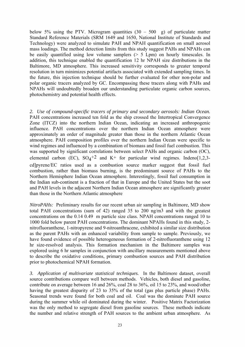
below 5% using the PTV. Microgram quantities (30 – 500 g) of particulate matter Standard Reference Materials (SRM 1649 and 1650, National Institute of Standards and Technology) were analyzed to simulate PAH and NPAH quantification on small aerosol mass loadings. The method detection limits from this study suggest PAHs and NPAHs can be easily quantified using low volume samplers (> 5 Lpm) on hourly timescales. In addition, this technique enabled the quantification 12 hr NPAH size distributions in the Baltimore, MD atmosphere. This increased sensitivity corresponds to greater temporal resolution in turn minimizes potential artifacts associated with extended sampling times. In the future, this injection technique should be further evaluated for other non-polar and polar organic tracers analyzed by GC. Encompassing these tracers along with PAHs and NPAHs will undoubtedly broaden our understanding particulate organic carbon sources, photochemistry and potential health effects. 2. Use of compound-specific tracers of primary and secondary aerosols: Indian Ocean. PAH concentrations increased ten fold as the ship crossed the Intertropical Convergence Zone (ITCZ) into the northern Indian Ocean, indicating an increased anthropogenic influence. PAH concentrations over the northern Indian Ocean atmosphere were approximately an order of magnitude greater than those in the northern Atlantic Ocean atmosphere. PAH composition profiles over the northern Indian Ocean were specific to wind regimes and influenced by a combination of biomass and fossil fuel combustion. This was supported by significant correlations between select PAHs and organic carbon (OC), elemental carbon (EC), SO4+2 and K+ for particular wind regimes. Indeno[1,2,3-cd]pyrene/EC ratios used as a combustion source marker suggest that fossil fuel combustion, rather than biomass burning, is the predominant source of PAHs to the Northern Hemisphere Indian Ocean atmosphere. Interestingly, fossil fuel consumption in the Indian sub-continent is a fraction of that in Europe and the United States but the soot and PAH levels in the adjacent Northern Indian Ocean atmosphere are significantly greater than those in the Northern Atlantic atmosphere NitroPAHs: Preliminary results for our recent urban air sampling in Baltimore, MD show total PAH concentrations (sum of 42) ranged 35 to 200 ng/m3 and with the greatest concentrations on the 0.14 0.49 m particle size class. NPAH concentrations ranged 10 to 1000 fold below parent PAH concentrations. The dominant NPAHs found in this study, 2-nitrofluoranthene, 1-nitropyrene and 9-nitroanthracene, exhibited a similar size distribution as the parent PAHs with an enhanced variability from sample to sample. Previously, we have found evidence of possible heterogeneous formation of 2-nitrofluoranthene using 12 hr size-resolved analysis. This formation mechanism in the Baltimore samples was explored using 6 hr samples in conjunction with ancillary measurements mentioned above to describe the oxidative conditions, primary combustion sources and PAH distribution prior to photochemical NPAH formation. 3. Application of multivariate statistical techniques. In the Baltimore dataset, overall source contributions compare well between methods. Vehicles, both diesel and gasoline, contribute on average between 16 and 26%, coal 28 to 36%, oil 15 to 23%, and wood/other having the greatest disparity of 23 to 35% of the total (gas plus particle phase) PAHs. Seasonal trends were found for both coal and oil. Coal was the dominate PAH source during the summer while oil dominated during the winter. Positive Matrix Factorization was the only method to segregate diesel from gasoline sources. These methods indicate the number and relative strength of PAH sources to the ambient urban atmosphere. As

24

with all source apportionment techniques, these methods require the user to objectively interpret the resulting source profiles. References 1. Grob, K. and Biedermann, M. (1996) Vaporizing systems for large volume injection or on-

line transfer into gas chromatography: classification, critical remarks and suggestions. Journal of Chromatography A, 750, 11-23.

2. Crimmins, B.S. and J.E. Baker. Measurement of aerosol PAH and nitro-PAH

concentrations in ambient urban air with hourly resolution, submitted to Atmos. Environ. 3. Bamford, H.A. and J.E. Baker (2003) Sources and concentrations of nitro-PAHs in urban

and sub-urban atmospheres of Maryland. Atmos. Environ., 37 (15): 2077-2091. 4. Crimmins, B.S., R.R. Dickerson, B.G. Doddridge and J.E. Baker (2004) Particulate

polycyclic aromatic hydrocarbons (PAHs) in the Atlantic and Indian Ocean atmospheres during INDOEX and AEROSOLs99: Continental sources to the marine atmosphere. J. Geophys. Res. Atmos., 109(D5), doi:10.1029/2003JD004192.

5. Larsen, R.K. and J.E. Baker (2003) Source apportionment of polycyclic aromatic

hydrocarbons in the urban atmosphere: a comparison of three methods. Environ. Sci. Technol., 37, 1873-1881.

25

ATMOSPHERIC CONCENTRATIONS IN AIR AND DEPOSITION FLUXES OF POPs IN NORTHERN EUROPE, TRENDS AND SEASONAL AND SPATIAL

VARIATIONS.

Eva Brorström-Lundén, Katarina Strömberg, Anna Palm Cousins and Jeanette Andersson Swedish Environmental Research Institute, IVL, P.O. Box 5302, 40014 Göteborg, Sweden Introduction Persistent organic pollutants (POPs) are subject to long-distance transport and are likely to bioaccumulate and may thus pose a risk to humans and wildlife in aquatic and terrestrial ecosystems both far from and close to source areas (UNEP 1998). The importance of atmospheric transport and deposition as a pathway for POPs to the Nordic environment as well as to the Arctic areas has been shown by different measurement activities and by model exercises (Stern et al., 1997, Harner et al., 1998, Hung et al., 2001, Kallenborn et al., 2002, Shatalov & Malachinev, 2000, UNEP 2002). In order to assess the importance of atmospheric transport and to quantify the regional atmospheric cycling of POPs, measurements are carried out. A further aim with measurements is to obtain information in order to develop a policy to reduce this pollution (emission control). In Sweden, measurements of selected POPs were included in the Swedish Monitoring Programme for Air Pollutants during 1995 at one station at the Swedish west coast. In 1996, a monitoring programme for POPs started at a station in a sub-arctic area. The monitoring program includes different classes of substances, such as polycyclic aromatic hydrocarbons (PAHs), polychlorinated biphenyls (PCBs), hexachlorocyclohexanes (HCHs). Measurements of brominated flame retardants (PBDEs) were added to the monitoring programme at the Swedish West Coast in 2001 and in Pallas in 2003. All the above mentioned substances are frequently present in the atmosphere and are of varying origin, i.e. they are emitted to the environment via industrial processes, combustion, end-use of products or agricultural use. In addition to the regular monitoring program, screening studies are carried out in Sweden. The aim with these studies is to investigate the presence and concentration levels of selected chemicals and to provide information about important transport pathways of the substance in the environment, e.g. atmospheric transport. The results of a screening may lead to the inclusion of new chemicals in the regular monitoring programs. Recently, a screening study of endosulfane and mirex was carried out and results are partly presented here. In this paper, the results from the measurements of POPs in air and deposition carried out between 1995 and 2004 at will be presented. Previously published data from the Swedish West Coast 1989-1994 have also been included in order to obtain a longer time-series. Seasonal and temporal trends will be discussed, as well as spatial variation in a European perspective. Results from screening studies will also be presented. The data summarised

26

and presented in here can also be found in the Swedish EPA’s database for air pollutants hosted by IVL (www.ivl.se). Material and Methods

The measurements of POPs have been carried out at two sites: Råö, which is an EMEP station (Co-operative Programme for Monitoring and Evaluation of the Long-Range Transmission of Air Pollutants in Europe) at the Swedish west coast (previously Rörvik) and Pallas, a monitoring station within AMAP (the Arctic Monitoring Assessment Programme). The sampling at Pallas is operated by the Finnish Meteorological Institute (FMI) and the measurements are performed in co-operation between Sweden and Finland. The sampling program includes parallel sampling of POPs in air and deposition with a frequency of one week per month and the sampling is undertaken simultaneously at the two sites. However in order to adopt the recommendations from EMEP, the sampling programme at Råö was extended in 2001 to weekly sampling in air and monthly sampling of deposition. POPs in air are collected using a high volume air sampler (HVS). A glass fiber filter is used for trapping the particles followed by an adsorbent of polyurethane foam (PUF) for collecting compounds in the gas phase. Both wet and dry deposition is collected using an open sampler (bulk sampler). This sampler consists of a 1 m2 Teflon coated surface with 10cm high edges. The bottom declines slightly to a central opening where a cassette with an adsorbent of PUF is attached. The deposition sample includes both compounds in the precipitation and compounds deposited to the collection surface of the sampler. Both the precipitation and the deposited particles are included in the analysis. At Pallas, a modified sampler is used for collection of POPs in the snow. The sampling and analytical methods are described elsewhere (Brorström-Lundén et al., 1995). Results and Discussion Atmospheric concentrations PAH and PCB The measured air concentrations of PAHs (sum 16) and PCBs (sum 7) at Råö and Pallas during the sampling occasions 1996 -2004 are summarised in figure 1. The data is illustrated using "box whisker plots". The boundary of the box indicates the 25th and 75th percentiles and the line within the box marks the median. Whiskers (error bars) above and below the box indicate the 90th and 10th percentiles. In addition, the average (red line) and outlying points are shown.

http://www.ivl.se/

27

The concentrations of PAH, PCB and HCH at

Figure 1. The atmospheric concentrations of PAHs and PCBs

The atmospheric concentrations of PAHs and PCBs have declined at the Swedish West Coast since 1989 (Brorström-Lundén, 1994). Since 1996, however, the concentrations of PAH and PCB at both Råö and Pallas seem to have leveled off and now remain on a fairly constant level (figure 1). The PAH concentrations were significantly lower in the north of Finland compared to the atmosphere of the Swedish West Coast, while the concentrations of PCBs at Pallas were somewhat lower or similar to those in southern Scandinavia. Figure 2 shows the seasonal variations at the Swedish West Coast during 2003 for two selected substances: Benzo(a)pyrene and PCB153.

Pallas air

Year

1994 1996 1998 2000 2002 2004 2006

pg/m

3

0

5

10

15

20

25

30

Sum 7 PCB

Råö air

Year

1996 1998 2000 2002 2004

ng/m

3

0

2

4

6

8

10

12

14

16

18

Sum PAH

Pallas

Year

1994 1996 1998 2000 2002 2004 2006

ng/m

3

0

1

2

3

4

Sum PAH

Råö air

Year

1994 1996 1998 2000 2002 2004 2006

/3

0

20

40

60

80

Sum 7 PCB

28

Figure 2. Atmospheric concentrations of Benzo(a) pyrene and PCB 153 at Råö. A seasonal variation in the atmospheric concentrations of PAHs was observed, with the highest concentrations during the winter periods. The concentrations also varied with the origin of air masses. The atmospheric concentrations of PCBs also varied with season and to some extent with the origin of air masses. The significant increase in atmospheric concentrations of PCBs during the warmer periods indicates that re-emission of PCBs back to the atmosphere takes place. This observation supports the theory of global fractionation of POPs (Wania and Mackay, 1996). Occasionally, elevated concentrations of both PAHs and PCBs were observed, which is exemplified with BaP and PCB 153 in figure 2. HCH The annual average concentrations of hexachlorocyclohexanes in the atmosphere are shown in Figure 3. Figure 3. Atmospheric concentrations of HCHs at Råö and Pallas (annual average concentrations). The atmospheric concentrations of both alpha- and gamma-HCH have decreased significantly at the Swedish West Coast since 1989 (Brorström-Lundén et al., 1994). The concentrations seem to decrease also in the time period 1996-2004 (figure 3). The concentrations of alpha-HCH are lower at the Swedish West Coast while the g-HCH concentrations are higher in at the west coast than in northern Finland. Like for PCBs, there was an increase in air concentrations during the spring and summer periods also for the HCHs. This is likely to be due to the consumption of the pesticides in southern countries, reaching Scandinavia via long-range atmospheric transport.

0.00

0.10

0.20

0.30

0.40

0.50

0.60

0.70

RA 01

RA 04

RA 07

RA 10

RA 13

RA 16

RA 19

RA 22

RA 25

RA 28

RA 31

RA 34

RA 37

RA 40

RA 43

RA 46

RA 49

Benso(a)pyrene ng/m32003

0.00

2.00

4.00

6.00

8.00

10.00

12.00

RA01

RA04

RA07

RA10

RA13

RA16

RA19

RA22

RA25

RA28

RA31

RA34

RA37

RA40

RA43

RA46

RA49

RA52

PCB 1532003pg/m3

0

10

20

30

40

50

60

1996

1998

2000

2002

2004

1996

1998

2000

2002

2004

g-HCHa-HCH

pg/m3

Råö Pallas

Yearly average of HCHs

29

PBDE The atmospheric concentrations of BDEs 47, 99 and 100 in 2003 and 2004 at the Pallas sampling station are shown in Figure 4.

Figure 4. Atmospheric concentrations of PBDEs at Pallas

A seasonal variation in atmospheric concentrations of PBDEs was observed at Pallas (Figure 4), with the highest concentrations in the summer. This was more obvious in 2004 than in 2003. The concentrations of PBDEs were similar at Råö as in Pallas, however the seasonal variation at the West Coast was less pronounced and an increase in concentrations during summer was found only during 2001. Endosulfan During 2004, endosulfan was included in a Swedish screening study and air was sampled both at Råö and Pallas. The results from these measurements are shown in Fugure 5.

JanJan

MayMay

Aug Aug

NovNov

Jan May

Aug Dec

Con

cent

ratio

n (p

g/m

3 )

0

2

4

6

8

10

12

14

16

18

20α-endosulfan β-endosulfan endosulfan sulphate α-HCHγ-HCH

Råö Pallas

0.00

0.50

1.00

1.50

2.00

2.50

3.00

jan-03

mar-03

maj-03

jul-03

sep-0

3

nov-0

3feb

-04ap

r-04jun

-04

sep-0

4ok

t-04

dec-0

4

PBDE-99PBDE-100PBDE 47

pg/m3

Pallas

30

Figure 5. Concentration of α-endosulfan, β-endosulfan and endosulfan sulphate, as compared to the HCH-levels at Råö and Pallas. At Råö, the endosulfan samples were taken over a whole month, whereas the HCH samples are two-week-samples, thus the graph shows two values for HCHs each month, but only one value for endosulfan. Figure from Palm Cousins et al. (2005). The concentrations of α-endosulfan at Råö were in the same range as both α-HCH and γ-HCH and showed a similar pattern of seasonal variation with higher concentration during the spring - summer, which may reflect the use of pesticides (endosulfan) in southern Europe (Figure 5). The concentrations of α-endosulfan at Pallas were lower compared to Råö, especially during the spring and summer periods, but very similar to the measured concentrations of γ-HCH (Palm Cousins et al., 2005).

Deposition fluxes

PAH and PCB The deposition fluxes of PAHs and PCBs are summarised in figure 6.

Figure 6. Deposition fluxes of PAH and PCB at Råö and Pallas between 1994 and 2003. The deposition fluxes at Råö were generally slightly higher or in the same order of magnitude as in Pallas. The greatest amounts of PAHs, and PCBs at the Swedish west coast were deposited in connection with high precipitation. The deposition fluxes are affected by long-distance sources and to some extent by local sources. The importance of long-range transport for the occurrence of POPs at remote sites is evidenced by the relatively high deposition fluxes of these pollutants also in Pallas. HCH and PBDE The deposition fluxes of γ-HCH were higher at the west coast compared to Pallas, whereas the deposition fluxes of α-HCH were similar in the south and north. The deposition of PBDEs was significantly higher in Pallas compared to Råö. Conclusions The atmospheric concentrations of POPs at the Swedish West Coast have declined since 1989, however, the concentrations of PAH, PCB and HCH at Rörvik and Pallas seem to have leveled off since about 1996 and remain on a fairly constant level.

0

0.05

0.1

0.15

0.2

0.25

0.3

0.35

0.4

0.45

1994

1996

1998

2000

2002

2004

1997

1999

2001

2003

Sum PAHug/m2 dayDeposition fluxes

Råö Pallas

0

0.5

1

1.5

2

2.5

1994

1996

1998

2000

2002

2004

1997

1999

2001

2003

Sum PCBng/m2 day Deposition fluxes

Råö Pallas

31

The PAH concentrations are significantly higher in the south of Scandinavia than in the north, whereas the concentrations of PCB, HCH and PBDEs are of similar order of magnitude in the north of Finland or even higher than the Swedish West Coast, which provides strong evidence for long-range transport of these compounds. The deposition measurements at Rörvik and Pallas show that significant amounts of POPs are deposited and the importance of long-range transport for the occurrence of POPs at remote sites is evidenced by the relatively high deposition fluxes of these pollutants also at Pallas.

The data in this report will be further evaluated.

Acknowledgements

The measurements at Rörvik are financed by the Swedish EPA and in Pallas by Swedish EPA together with the Norrbotten County

References

Brorström-Lundén E. 1995. Measurements of Semivolatile Organic Compounds in Air and Deposition. Ph.D thesis April 1995 Department of Analytical and Marine Chemistry University of Göteborg. Brorström-Lundén E., Lindskog A and Mowrer J. 1994. Concentrations and Fluxes of Organic Compounds in the Atmosphere of the Swedish west coast. Atmos. Environ. 28, 36053615 Harner T., Kylin H., Bidleman T. F., Halsall C., Strachan W. M. J., Barrie L. A., Fellin P. 1998. Polychlorinated Napthtalenes and Coplanar Polychlorinated Biphenyls in Arctic Air. Environmental Science and Technology 32, 3257-3265 Hung H., Halsall C.J., Blanchard P., Li H.H., Fellin P., Stern G., Rosenberg B. 2001. Are PCBs in the Canadian Arctic Atmosphere Declining? Evidence from 5 years of Monitoring. Environmental Science and Technology 35, 1303-1311 Kallenborn R, Blanchard P., Hung H., Muir D., Olafsdottir K., Brorström-Lundén E., Leppanen S. Manø S. (2002) Trends and levels of persistent organic contaminants in the Arctic atmosphere Pesentation at the AMAP-Symposium in Rovaniemi 1-4.10.2002. Palm Cousins A., Remberger M., Andersson J., Kaj L., Strömberg K., Ekheden Y., Dusan B., Cato I., Brorström-Lundén E. 2005. Results from the Swedish National Screening Programme 2004 Subreport 5: Mirex and Endosulfan. IVL report, B1641 Shatalov V., Malanichev A. 2000. Investigation and assessment of POP transboundary transport and accumulation in different media. Part II. MSCE-E EMEP Report 4/2000 Stern G. A., Halsall C. J., Barrie L. A., Muir D. C. G., Fellin P., Rosenberg B., Rovinsky F. YA., Kononov E. YA., Pastuhov B. 1997. Polychlorinated Biphenyls in Arctic Air. 1. Temporal and Spatial Trends: 1992-1994. UNEP 1998. Document UNEP/POPS/INC.1/6. 30 April 1998

32

UNEP 2002. Regionally Based Assessment of Persistent Toxic Substances. Europe Regional Report., UNEP Chemicals, Switzerland, December 2002 Wania F., Mackay D. 1996. Tracking the distribution of persistent organic pollutants. Environmental Science and Technology 30. 390A-396A

33

POPs AIR STUDIES IN CENTRAL AND SOUTHEASTERN EUROPE (RECETOX ACTIVITIES)

Ivan Holoubek, Jana Klánová

RECETOX – TOCOEN & Associates (RECETOX, Masaryk University Brno + TOCOEN,

s.r.o., Brno), Czech Republic

EUROPEAN REGIONAL BACKGROUND MONITORING OF POPS (the Results from Long-term Integrated Monitoring, Košetice Observatory, CR, 1988 – 2005) Introduction Persistent organic pollutants (POPs) in all environmental matrices are monitored in the area of Košetice observatory (professional observatory of Czech Hydrometeorological Institute located in south Bohemia) since the 1988. Observatory is developed as EMEP regional background monitoring site in the Central Europe. Observatory is included among regional background stations under both international (GAW, EMEP) and national programmes. The monitoring of POPs is performed on the base of integrated monitoring approach1. The regional and global nature of the processes makes international efforts to generate comparable measurements the only basis on which further knowledge on the pools and fluxes can rest. Only a few POPs had been measured at a few sites. The overall aim of integrated monitoring was originally to determine and predict the state and change of terrestrial and freshwater ecosystems in a long-term perspective with respect to the impact of air pollutants including persistent organics (IM EMEP). Integrated monitoring of ecosystems means physical, chemical and biological measurements over time of different ecosystem compartments simultaneously at the same location. A small catchment (or other hydrological well defined area), such as in integrated monitoring site, is large enough to encompass all the interacting components: atmosphere and vegetation, plants and soils, bedrock and groundwater, brook or lake, and surrounding land. Methods The regional background monitoring of POPs is a part of two research projects of RECETOX. The first is a Project TOCOEN (Toxic Organic Compounds in the Environment) (which started in 1988) and project INCHEMBIOL (Interactions among the chemicals, environment and biological systems and their consequences on the global, regional and local scales) (realized from 2004). This POPs monitoring at Košetice is a part of long-term co-operation between Czech Hydrometeorological Institute and RECETOX – TOCOEN & Associates. The philosophy is based on the main approaches of EMEP strategy in field of POPs measurements2.

In present time, the POPs monitoring programme at Košetice observatory has been carried out on a regular basis for already 17 years – a unique achievement globally. The sampling procedure, analytical determination and QA/QC are based on the recommendations of the EMEP. Pollutants are described in Table 1 and basic details of sampling procedures in Tables 2 and 3.

34

Table 1: Model pollutants

PAHs (16 by US EPA) PCBs seven indicator congener, IUPAC number 28, 52, 101, 118, 153, 138, 180

Hexachlorobenzene (HCB), pentachlorobenzene (PeBZs) α,β, γ,δ-Hexachlorocyclohexanes (HCHs)

DDT, DDE, DDD Table 2: The basic characteristics of ambient air and wet deposition sampling

Ambient air Wet deposition Sampler High volume Collection vessel

operated manually Conditions of sampling

Recommended flow and volume: 20-25 m3.h-1 and 500 m3 per samples

Sampling area: 0.75 m2

Phases Gas and particles Sorbents Glass or quartz filter and solid

adsorbent trap (polyurethane foam) Silica

Frequency of sampling

24 hours measurements one per week (Wednesday, 08.00 – Thursday, 08.00)

After every event

Extraction Soxhlet extraction LLE Analysis PAHs, OCPs, PCBs: GC-MSD

Table 3: The basic characteristics of surface waters, sediments, soils and plants sampling

Surface waters

Sediments Soils Plants

Sampling sampling bottle

humus, mosses, needles

Sampling volume 1 l Sampling procedure: Manual of ICP IM

Sampling layer 0-10 cm 0-10 cm Collection period once per year Extraction LLE Soxhlet extraction Analysis – GC-MSD

PAHs, OCPs, PCBs

Results and discussion Trends in the development of the medians of regional background concentrations of the mentioned pollutants are shown in the graphs in Figures 1 (PAHs, PCBs, DDTs, HCHs and HCB) and document the slightly decreasing tendency of monitored pollutants on a regional level but with respect to the local situation. The increase of the ambient air concentrations of PAHs reflects the return of coal combustion in local heating systems as a result of the economic situation. Changes in the annual medians of PCBs and OCPs reflect the results of floods in the CR (1997 and 2002). The PAHs concentrations identified follow characteristic course prompted by the higher occurrence of these compounds in winter when they are produced by various combustion processes. PCBs and OCPs concentrations display a totally different profile in which no such “seasonality” has been identified. These compounds are present in the atmosphere today due to their volatilisation from soil and sediments, i.e. as secondary inputs from old

35

deposits, and also due to a long-range atmospheric transport from regions in which they are still used. PCBs occurrence remains at the level of the European background. From the PCBs pictures we can see the decreasing tendency during this period. Predominance of degradation metabolites of DDT (DDE and DDD) was observed (the same trend exists in all environmental samples from this observatory)3. This predominance reflected old loads – input from old usage and environmental accumulation of DDT rather than long-range transport from regions where the compound is still in use4. Figure 1: Trends in the development of medians of regional background concentrations of PAHs, PCBs, DDTs, HCHs and HCB in ambient air, observatory Košetice, 1996-2004 [ng.m-3]

Air (Aerosol + Gas Phase), Σ PAHs medians, Košetice, CR

0

5

10

15

20

25

1996 1997 1998 1999 2000 2001 2002 2003 2004

Years

ng.m

(-3)

Air (Aerosol + Gas Phase), Σ PCBs medians, Košetice, CR

0

0,05

0,1

0,15

0,2

1996 1997 1998 1999 2000 2001 2002 2003 2004

Years

[ng.

m(-

3)]

Air (Gas phase + Aerosol), Σ DDTs medians, Košetice, CR

0

0,01

0,02

0,03

0,04

0,05

0,06

1996 1997 1998 1999 2000 2001 2002 2003 2004

Years

[ng.

m(-

3)]

Air (Gas Phase + Aerosol), Σ HCHs medians, Košetice, CR

0

0,02

0,04

0,06

0,08

0,1

0,12

1996 1997 1998 1999 2000 2001 2002 2003 2004

Years

[ng.

m(-

3)]

Air (Gas Phase + Aerosol), HCB medians, Košetice, CR

0

0,05

0,1

0,15

0,2

0,25

1996 1997 1998 1999 2000 2001 2002 2003 2004

Years

[ng.

m(-

3)]

Conclusions Long-term monitoring of POPs in observatory Košetice is a useful tool for the study of environmental processes and temporal and spatial trends of these compounds. The decreasing trends of environmental levels of POPs in the region of Central Europe were/are observed. The results of this monitoring are useful base for validation of distribution models (in co-operation with EMEP MSC East, Moscow, Russia).

36

SUBREGIONAL AND LOCAL MONITORING AND RESEARCH PROJECTS (CZECH REPUBLIC, BALKAN COUNTRIES) (1993-2005) ACTIVE SAMPLING CAMPAIGNS1,5

RECETOX was/is performed few other active sampling campaigns in few regions in the Czech Republic and in the countries of former Yugoslavia. Czech Republic

- RECETOX study area - region Zlin, eastern Moravia, measurements of POPs (PAHs, PCBs, OCPs, PCDDs/Fs) + VOCs - HMs, 1993-2005 - few days or week sampling campaigns per year - 5-8 sampling sites + soils (10-30 sampling sites) + sediments (round 15 sites)

- Episodic campaigns - Beroun - small industrial town near to Prague - 2002 - 3 one week sampling campaigns - PAHs, PCBs, OCPs, PCDDs/Fs

- National monitoring of PAHs realized by Czech Hydrometeorological Institute - 20 sampling sites, every week + similar by State Institute of Health

Former Yugoslavia The first systematic ambient air sampling campaigns for POPs analyses were performed in Croatia, Serbia, Bosnia and Herzegovina5. Data will be useful contribution not only to this project, but also for ongoing national POPs inventories as a part of implementation of Stockholm convention. High volume air sampling in 25 selected sites in Croatia, Serbia, Bosnia and Herzegovina jeopardized by destruction of natural resources, infrastructure, and enterprises was performed in the first two years of the project. Air sampling and analysis were performed by RECETOX and sampling sites were selected in co-operation with the partners. The concentrations of PCB congeners, OCPs and PAHs in the gaseous and particulate phases of the air samples were determined. During the ambient air sampling campaign, samples of surface soil were collected close to the site of the atmospheric sample collectors. RECETOX has participated on the 5th EU Framework Programme - project APOPSBAL (EU Project ICA2-CT2002-10007 “Assessment of the selected POPs in the atmosphere and water ecosystems from the waste generated by warfare in the area of formal Yugoslavia”) and 3 sampling campaigns with using of active samplers were realized:

- 2002 - Zadar, Croatia - 4 sampling sites in Zadar + 1 in Zavizan - 1 700 m a.s.l. - background observatory, 1 week campaigns, 24 hrs sampling period

- 2002, 2003 - Serbia - Kragujevac, Pancevo, Novi Sad - total 9 sampling sites, usually 3 days sampling campaigns on every site, 24 hrs sampling period

- 2004 - Bosna and Herzegovina - Sarajevo, Tuzla - sampling sites in every town, one week sampling campaigns, 24 hrs sampling period AIR PASSIVE SAMPLING6-10 RECETOX performed during last two years a lot of research work in the field of application of passive air samplers, which were focused on the determination of conditions affected the sampling process (sampling volume, effects of wind, temperature, construction of sampler), determination of local conditions on sampling and study of temporal and spatial variations of POPs in selected sites of the Czech Republic and countries of former Yugoslavia (Croatia, Serbia, Bosnia). In the comparison with other groups, RECETOX has now very broad set of data from application of passive samplers

37

(round 60 sampling sites with sampling duration from 5 months to 2 years and using of 28 days sampling frequency). The aim of one study6 was to investigate the potential of passive air sampling devices to assess the influence of local sources on the quality of surrounding environment. It was focused on the sensitivity of this technique to the seasonal and spatial variations in the ambient air concentrations of persistent organic compounds (POPs). Passive air samplers were employed for the purpose of two case studies in the Czech Republic. DEZA Valašske Meziříčí, a coal tar and mixed tar oils processing plant, and Spolana Neratovice, a chemical factory with the history of high production of organochlorine pesticides (OCPs), were selected as the point sources of PAHs, and OCPs, respectively. Ten sampling sites in different distances and directions from each point source were selected and they have been monitored for six months. Polyurethane foam filters in sampling devices were replaced every 28 days during the campaign lasting from January to July 2004. Levels of PCBs, OCPs and PAHs were determined for all sampling sites and sampling periods. The study brought useful data about the air concentrations of POPs in the investigated regions. More important, it provided information on the transport and fate of POPs in the vicinity of local sources of contamination useful for the estimation of their influence. Very good capability of passive samplers to reflect temporal and spatial fluctuation in concentrations of persistent organic pollutants in the ambient air was confirmed which makes them applicable for monitoring on the local scale. It was demonstrated previously7-10 that passive air samplers using PUF filters are suitable to study vapor-phase air concentrations of some types of POPs, particularly more volatile compounds from the group of polycyclic aromatic hydrocarbons, polychlorinated biphenyls and organochlorine pesticides, and they were successfully applied as a tool for POPs monitoring on the global and regional levels. The RECETOX study suggests they are sensitive enough to mirror even small-scale differences, which makes them capable of monitoring of spatial, seasonal and temporal variations. Passive samplers can be used for point sources evaluation in the scale of several square kilometers or even less - from the local plants to diffusive emissions from transportations or household incinerators - as well as for evaluation of diffusive emissions from secondary sources. While not being sensitive to short time accidental releases passive air samplers are suitable for measurements of long-term average concentrations at various levels. On the other hand, this sensitivity to local effects can lead to some limitations toward its application in large-scale monitoring. Sampling site selection seems to be crucial for the success of such projects since small-scale variability in each region can exceed the continental variability. To develop a monitoring network, the local conditions must be evaluated very carefully since only detail characterization of potential local effects for every sampling site can assure the successful selection of sites for larger (regional or global) scale monitoring. Very good capability of passive air samplers to reflect temporal and spatial fluctuation in concentrations of persistent organic pollutants in the ambient air was confirmed in this study. While this sensitivity makes them suitable for the monitoring of local sources, it also needs to be considered when designing large scale monitoring networks. The aim of the second RECETOX study11 was to investigate the capability of passive air sampling technique to be employed in the evaluation of direct genotoxicity of ambient air samples. Genotoxic effects of the total extracts from the polyurethane foam filters exposed for 28 days during the regional passive air sampling campaign were investigated.

38

Twenty sampling sites were selected in Brno city on the area of approximately 20x20 km in October and November 2004. Brno is the second largest city of the Czech Republic, highly industrialized with approximately 370 000 of permanent inhabitants. The levels of polycyclic aromatic hydrocarbons, polychlorinated biphenyls, and chlorinated pesticides were determined in all samples. In a parallel arrangement a fraction of each extract was assayed in the bacterial genotoxicity test using the Escherichia coli sulA::lacZ. Complete dose-response relationships of the air extracts were determined. Results of this study indicate not only a very good capability of the passive air samplers to reflect the spatial fluctuation in concentrations of persistent organic pollutants in the ambient air but the feasibility of using this method for the direct genotoxic potential assessment. The integration of the passive air sampling technique with the genotoxicological analysis may provide an effective tool for the air monitoring on various scales and for the screening of the genotoxic potential of ambient air samples which can be used for exposure assessment as a part of human health risk assessment. Application of passive samplers in APOPSBAL Project Third year of APOPSBAL project, a passive air sampling method was used12-14. The aim of the APOPSBAL project was to map the situation with the POPs contamination of former Yugoslavian countries, find possible hotspots, evaluate the risks, and suggest suitable remediation activities. The application of passive samplers was a suitable tool for the realisation of this approach. Determination of the polychlorinated biphenyls, organochlorinated pesticides, and polyaromatic hydrocarbons in the atmosphere was performed. In order to better compare data from different sampling events, to collect the samples from remote places, as well as to gain more information about the spatial and temporal distribution of POPs, additional passive air sampling (PAS) campaign was organized in Croatia, Serbia, Bosnia, Herzegovina, and Kosovo in 2004. PUF based passive samplers were employed at 34 sampling sites for 5 consecutive periods of 28 days. The network was based on the results of previous high volume ambient air sampling campaigns. Industrial, residential, as well as background areas were included. Some background sites were added to the list of locations to learn more about spatial variations, as well as several sites where active air sampling proved to be difficult to organize (Kosovo, Western Slavonia). Additional twenty sampling sites in the Czech Republic served as a reference region, including the background observatory Košetice serving as EMEP observatory 10.

Results of the passive air sampling campaign were in very good agreement with the previous high volume measurements. The samples of the top soil layer were taken close to all passive air sampling sites.

Results of the passive air sampling campaign were in very good agreement with the previous high volume measurements. Decreasing trend in the levels of PCB and OCP contamination from July to December corresponds with decreasing temperature and indicates enhanced evaporation from secondary sources during the warm season. PCB congener pattern was investigated as well. Again, passive and active samplings gained very similar information about the congener distribution. The samples of the soil top layer were taken close to all passive air sampling sites. Significant correlation between both, the PCBs levels in the atmosphere and in the soil surface, and between the congener distribution in the air and soil, was found.

Also new types of pollutants for example short chains chlorinated paraffins were/are determined in the ambient air samples from active and passive samplers as well15,16.

39

POPs IN SOIL - VOLATILISATION RECETOX has a relatively good set of results concerning to POPs soil contamination which are applicable for the study of volatilization and air/soil exchange. The contents of POPs - PAHs, OCPs (DDTs HCHs, HCB, driens, toxaphen), PCBs and PCDDs/Fs from round 200 sampling sites are available17. The results concerning to soil contamination by POPs in the countries of former Yugoslavia was mentioned above. One new special study, concerning to air/soil and air/plants exchange in the area of former OCP producer well known Spolana Neratovice is now realized by RECETOX18. Acknowledgement The research reported here was supported was supported by EU Project ICA2-CT2002-10007 “Assessment of the selected POPs in the atmosphere and water ecosystems from the waste generated by warfare in the area of formal Yugoslavia”, EUDG Centre of Excellence EVK1-CT-2002-80012, and Ministry of Education of the Czech Republic Project MSM 0021622412 INCHEMBIOL. References [1] Holoubek, I.: Monitoring, modelling and information system for persistent organic pollutants.

In: Prastacos, P., Cortés, U., de Leon, J. L. D., Murillo, M. (Eds.): e-Environment: Progress and Challenges. Research on Computing Science. Vol. 11, 117-134, IPN CIC Mexico, 2004. ISBN: 970-36-0215-0, ISSN: 1665-9899.

[2] Holoubek, I., Ansorgová, A., Kohoutek, J., Kořínek, P., Holoubková, I. (2000): The regional background monitoring of POPs (PAHs, PCBs, OCPs) in the Czech Republic. Organohal. Compounds. 46, 387-390

[3] Holoubek, I., Ansorgova, A., Shatalov, V., Dutchak, S., Kohoutek, J. (2001): Regional background monitoring of PBT compounds. The comparison of the results from measurements and monitoring. Environ. Sci. Pollut. Res. 8, 201-211 (2001).

[4] Holoubek, I., Klanová, J., Kohoutek, J. (2005): Regional background monitoring of POPs – the results from long-term integrated monitoring, Kosetice observatory, CR, 1988 - 2005. Organohl. Compounds

[5] Picer, M., Picer, N., Holoubek, I., Klanova, J., Kobasic, V.H. (2004): Chlorinated hydrocarbons in the atmosphere and surface soil in the areas of the city of Zadar and Mt. Velebit Croatia. Fresenius Environ. Bull., 3(8), 712-718.

[6] Klánová, J., Kohoutek, J., Hamplová, L., Urbanová, P., Holoubek, I.: Passive air sampler as a tool for long-term air pollution monitoring: Part 1. Performance assessment for seasonal and spatial variations. Environ. Pollut. (submitted)

[7] Harner, T., Shoeib, M., Diamond, M., Stern, G., Rosenberg, B. (2004): Using passive air samplers to assess urban - Rural trends for persistent organic pollutants. 1. Polychlorinated biphenyls and organochlorine pesticides. Environ. Sci. Technol. 38, 4474-4483.

[8] Jaward, F. M., Farrar, N. J., Harner, T., Sweetman, A. J., Jones, K. C. (2004): Passive air sampling of PCBs, PBDEs, and organochlorine pesticides across Europe. Environ. Sci. Technol. 38, 34-41.

[9] Jaward, F. M., Farrar, N. J., Harner, T., Sweetman, A. J., Jones, K. C. (2004): Passive air sampling of polycyclic aromatic hydrocarbons and polychlorinated naphthalenes across Europe. Environ. Toxicol. Chem. 23, 1355-1364.

[10] Jaward, F. M., Meijer, S. N., Steinnes, E., Thomas, G. O., Jones, K. C. (2004): Further studies on the latitudinal and temporal trends of persistent organic pollutants in Norwegian and UK background air. Environ. Sci. Technol. 38, 2523-2530.

40

[11] Čupr, P., Klánová, J., Bartoš, T., Flégrová, Y., Kohoutek, J., Holoubek, J.: Passive air sampler as a tool for long-term air pollution monitoring: Part 2. Air genotoxic potency screening assessment. Environ. Pollut. (submitted)

[12] Klánová, J., Holoubek, I., Kohoutek, J. (2005): POPs contamination of Balkan countries as a consequences of war damages: passive air sampling network. Organohal. Compounds

[13] Klánová, J., Holoubek, J., Kohoutek, J., Kostrhounová, R.: POPs contamination of atmosphere and soils in former Yugoslavian countries as a result of Balkan wars (submitted ES&T)

[14] Klánová, J., Holoubek, I., Kohoutek, J., Kostrhounová, R.: Passive air sampling network in Central and Southern Europe as a tool for a study of POPs contamination of Western Balkan countries as a consequences of war damages (submitted ES&T)

[15] Přibylová, P.: Determination of short chain chlorinated paraffins in environmental samples. PhD Thesis, RECETOX, Masaryk University, Brno, CR, September 2005.

[16] Přibylová, P., Klánová, J., Holoubek, I.: Contamination of the ambient air in Western Balkan countries by short and medium chain chlorinated paraffins (in preparation)

[17] Holoubek, I., Hofman, J., Sáňka, M., Vácha, R., Zbíral, J., Klánová, J., Jech, L., Ocelka, T. (2003): Spatial and temporal trends in persistent organic pollutants soil contamination in the Czech Republic. Organohal. Compds., 62, 460-463.

[18] Holoubek, I., Čupr, P., Jech, L., Ocelka, T., Kužílek, V., Vácha, R., Škarek, M., Matoušek, J., Kočan, A (2003): PCDDs/Fs contamination of the surroundings of Spolana Neratovice before and after floods 2002. Organohal. Compds., 61, 353-356.

41

THE NORTH AMERICAN GREAT LAKES’ INTEGRATED ATMOSPHERIC DEPOSITION NETWORK

Ronald A. Hites

School of Public and Environmental Affairs, Indiana University, Bloomington, IN 47405

The Great Lakes basin is home to 18% of the world’s freshwater supply and more than 10% of the United States and 25% of the Canadian populations (1). Economic activity in the region accounts for approximately 18% of the combined gross domestic products of the United States and Canada (2, 3). These facts alone make the environmental health of the Great Lakes important, and indeed, the Great Lakes have been the focus of early, classic water pollution studies. Starting in the late 1980’s, as point sources were brought under control, suspicions were raised that toxic substances were entering the lakes by deposition from the atmosphere. This would mean that, along with sources inside the basin, airborne pollutants from outside of the Great Lakes basin were a source of contaminants to the lakes (4). To study the scope of this problem, a workshop was held in 1986. Sponsored by the International Joint Commission, it produced a document (5) confirming that atmospheric deposition was a major source of contamination to the Great Lakes. This report led to Annex 15 in the 1987 revisions to the Great Lakes Water Quality Agreement of 1978 (6). This annex called for the creation of a network to measure the atmospheric concentrations of toxic substances near the Great Lakes. As a result, the Integrated Atmospheric Deposition Network (IADN) was created in 1990. Over its 15-year lifetime, IADN has determined that the Great Lakes have indeed been threatened by the deposition of many airborne toxic pollutants. However, these same long-term measurements indicate that this threat has diminished for many of these substances as regulations restricting their use take effect. IADN is a joint venture of Environment Canada and the United States Environmental Protection Agency’s Great Lakes National Program Office. IADN consists of a system of five master monitoring stations located on each of the five Great Lakes and several satellite stations (see Figure 1). IADN collects gas- and particle-phase air samples every 12 days for 24 hours at all master and at some satellite sites using high volume air samplers. Precipitation samples are taken during every rain or snow event and composited every 28 days (every 14 days at the Canadian sites) using wet-only precipitation samplers. Meteorological data such as air temperature and wind speed and direction are also collected at the sites and averaged on an hourly basis. IADN now measures 17 polycyclic aromatic hydrocarbons (PAHs), 22 organochlorine pesticides (those that are both banned and in-use), 56 polychlorinated biphenyls (PCBs), and 15 polybrominated diphenyl ethers. Chemical analysis is done by gas chromatographic mass spectrometry, gas chromatography with electron capture detection, and liquid chromatography with fluorescent detection. IADN features extensive quality assurance/quality control (QA/QC) procedures. These include laboratory and field blanks and duplicates, matrix spike experiments, and round-robin studies (7). Details on the sampling and analytical procedures can be found on the IADN website at http://www.smc-msc.ec.gc.ca/iadn/resources/resources_e.html. This abstract presents some of IADN’s current results and provides Internet links so that the interested reader can obtain more details. The actual data are also available to the scientific community by way of the IADN

http://www.smc-msc.ec.gc.ca/iadn/resources/resources_e.html

http://www.smc-msc.ec.gc.ca/iadn/resources/resources_e.html

42

web site’s data request form, which is at http://www.msc.ec.gc.ca/ iadn/data/form/form_e.html.

1.

Figure 1. Map of IADN sites. Master stations are the main sites in the network, and they were the first to be established for each lake. IADN added (and removed) satellite stations throughout the project to augment the master stations.

Temporal Trends One of the goals of IADN is to determine if the concentrations of toxic organic compounds are changing as a function of time in air and precipitation collected near the Great Lakes. Understanding these temporal trends is important both scientifically and politically, because trends can help researchers determine if and how fast the atmospheric concentrations are decreasing and provide clues about the sources of a chemical to the environment. Temporal trends can also help policy makers determine if their bans or restrictions on the use of a given chemical are working and how long it will take before these chemicals are eliminated from the environment. The use of many of the chemicals measured by IADN has either been banned or heavily restricted. One such chemical is α-hexachlorocyclohexane (α-HCH), which was a component (about 60% by weight) of technical HCH. This latter material was a mixture of five isomers of HCH, and it was used as a broad-spectrum insecticide starting in 1942. The use of technical HCH has since been banned, restricted, or de-registered in 70 countries, including the United States and Canada, where all registrations of this product were cancelled in 1978. Thus, by examining the temporal trend of α-HCH at each of the Great Lakes, we can determine if this ban on technical HCH has been effective. Figure 2 shows the gas-phase, annual-average concentrations of α-HCH from each IADN master station beginning in 1991. It is apparent from Figure 2 that there has been a dramatic decline in α-HCH concentrations in the air near each lake in the past 14 years. If the total loss rate of a given compound from the atmosphere is proportional to the amount of that compound in the atmosphere at any moment, then one would expect that the concentrations should follow a first-order rate law, Ct = C0 e-kt, where Ct is the atmospheric

http://www.msc.ec.gc.ca/ iadn/data/form/form_e.html

http://www.msc.ec.gc.ca/ iadn/data/form/form_e.html

43

concentration at time t, and k is a first order rate constant. We fitted the average annual concentration of all sites for each year in Figure 2 to this equation and obtained a rate constant of 0.17 yr-1 for the basin (see the line in Figure 2), which gives an overall environmental half-life of approximately 4 years for α-HCH in the air near the Great Lakes. In other words, we expect that the atmospheric concentrations of α-HCH near the Great Lakes will decrease by a factor of two every 4 years. Assuming first-order kinetics and minimal future inputs, we can use this temporal information to estimate a virtual elimination date (8) for α-HCH. This is the time when we will no longer be able to detect this compound in the atmosphere. Using the data in Figure 2 and a minimally detectable concentration of 0.1 pg/m3, this date works out to be about the year 2040, an indication that these compounds will be with us until well after most of us retire.

19911992

19931994

19951996

19971998

19992000

20012002

20032004

Con

cent

ratio

n (p

g/m

3 )

0

100

200

300

400

Lake SuperiorLake MichiganLake ErieLake HuronLake OntarioOverall trend

Figure 2. Annual average atmospheric gas-phase α-HCH concentrations in pg/m3 at each IADN master station from 1991 to 2004. Data for Lakes Huron and Ontario are not yet available for 2004. The Canadian concentrations were increased by a factor of 3.1 to compensate for analyte breakthrough on the collection media. Error bars are the standard error of each average.

Other banned pesticides and PCBs follow similar declining concentration patterns, but the virtual elimination dates differ for each substance (8-17). In contrast, PAHs are still being released into the atmosphere, mainly as the byproducts of fossil fuel combustion, and as a result, PAHs do not show declining concentration trends and generally have maintained their levels in the Great Lakes atmosphere over time. Spatial Trends Another goal of IADN is to determine the spatial trends of atmospheric pollutants in the Great Lakes basin. This analysis can help to determine where problems remain for certain substances and how the physical differences in the lakes and areas surrounding each lake affect atmospheric pollution levels. PCBs provide a good example of this approach. IADN data show that the total PCB concentrations at Chicago have been about an order of magnitude higher than at all of the other sites. PCBs were used in a wide array of industrial applications from 1930 to 1976, when their use was banned in the United States. Because their use was concentrated in urban areas, we expected to find Chicago’s PCB levels to be higher than those at IADN’s other sites, which are remote from major

44

population centers. Our second urban site, Cleveland, shows the second highest annual average total PCB concentrations. Not all of these remote sites, however, are immune to urban influences. For example, the IADN site at Sturgeon Point, near eastern Lake Erie, consistently has the third highest total PCB annual average, while the PCB concentrations for the other sites tend to be similar to one another. Sturgeon Point, although considered a remote sampling site, is located approximately 20 km southwest of Buffalo, NY, a relatively large urban center. Thus, even at this distance, there is an “urban effect” on the PCB concentrations at Sturgeon Point. Our studies of particle-phase PAH concentrations at Sturgeon Point have also shown that the PAH levels there were higher than at the other master stations (16). In fact, detailed analysis indicated that, when the winds blew from Buffalo toward the Sturgeon Point site, the PAH concentrations at this site were especially elevated (16). We can infer from these findings that Buffalo, NY is a source of PAH to the Sturgeon Point location, as it was for PCBs. Clearly, PAHs and PCBs are largely urban pollutants, which can travel tens of kilometers through the atmosphere. It is important to note, however, that increased urban concentrations are not found for all pollutants. For example, pesticide concentrations tend to be similar between remote and urban sites, presumably because the use of such chemicals was (or is) mainly agricultural. Nonetheless, the relative lack of urban sites in IADN represents a gap in our spatial understanding of air toxics around the basin, and for this reason, we added Cleveland, Ohio, in 2003. We have recently implemented a probabilistic model, called the potential source contribution function (PSCF), to estimate atmospheric source regions of PAHs, chlorinated pesticides, and PCBs to the Great Lakes (17). This model allows us to map each compound’s source region on a 0.5˚ × 0.5˚ latitude/longitude grid centered over the Great Lakes basin. PCBs primarily have urban sources, the strengths of which vary. Like PCBs, PAH show a strong urban signature, but these compounds also seem to come from rural sites. The source regions of PAH become less distinct as the molecular weight of the compound increases. Since reactivity increases with PAH size, this diminishing trend may be an indication that atmospheric degradation plays a large role in PAH transport. The pesticides have the strongest source regions and are typically transported the farthest, often from areas distant from the Great Lakes basin. Loadings IADN also determines loadings of these toxic compounds to the Great Lakes to fulfill another goal of the network. In this context, “loadings” means an estimate of the amount of a substance being deposited to the waters of the Great Lakes from the atmosphere minus the amount of that substance being volatilized or released from the water to the atmosphere. To make these estimates, IADN calculates wet deposition, dry deposition, gas absorption, and volatilization of the various substances using IADN atmospheric concentration data collected each year and using water concentration data for the Great Lakes measured by other researchers. Loadings estimates have been published for data from 1991-2000 in two-year increments (18-23). We have recently calculated a Great Lakes system-wide loading estimate by summing the total deposition for each substance across all five lakes (when available) for each year (24). Figure 3 shows these total regional loadings for total HCHs and for total PCBs. As

45

previously mentioned, α-HCH is a banned pesticide, while γ-HCH is currently in use only in the U.S., although its use is heavily restricted. Figure 3 shows that the total deposition of α- and γ-HCH into the Great Lakes has greatly decreased since 1992. On the other hand, region-wide loading estimates for in-use chemicals, such as PAHs and metals, show no real declining trend. These in-use chemicals continue to have many anthropogenic sources, allowing them directly to enter the atmosphere, which transports them to the Great Lakes, where they deposit.

19911992

19931994

19951996

19971998

19992000

2001

Tota

l dep

ositi

on (k

g/yr

)

-8000

-6000

-4000

-2000

0

2000

4000

6000total HCHstotal PCBsHCH trendPCB trend

Figure 3. Annual loadings for total HCHs (sum of the α and γ isomers) and total PCBs into or out of the five Great Lakes collectively. Loadings are presented as total deposition in kg/year. Total deposition is the sum of wet and dry deposition and gas absorption, minus volatilization. Negative total depositions indicate that, overall, the lakes are volatilizing the compound into the atmosphere. The two curves indicate general trends in the HCH and the PCB loadings.

PCB loadings to the Great Lakes as a function of time are also shown in Figure 3. In this case, we find that the waters of the Great Lakes have been volatilizing PCBs into the atmosphere for at least 9 years (this is the meaning of negative loadings) and that the rate of volatilization has generally decreased with time. Clearly, when PCBs had been in use in the 1960s, there were substantial inputs of these compounds into the lakes. Now that PCBs have been banned and the atmospheric concentrations have decreased, the air-water equilibrium has shifted, and the water is releasing its stores of PCBs back into the atmosphere. As indicated by the two curves in Figure 3, the deposition of HCHs into the lakes and the evaporation of PCBs from the lakes seem to be approaching zero. Because these compounds are relatively volatile and have little or no dry or wet deposition into the lakes, we know that the total deposition shown in Figure 3 is driven almost entirely by air-water exchange. This observation suggests that air-water partitioning, at least for these compounds, is approaching equilibrium. These findings, along with other IADN studies, suggest that the restrictions on the use of PCBs and of other chlorinated pesticides have helped to reduce their levels in the Great Lakes atmosphere and water, providing a healthier ecosystem for all inhabitants of the basin.

46

Summary The information presented here provides only a few examples of the work IADN has done to achieve its goals. Temporal trend studies have established that the concentrations of some banned substances continue to decrease over time at varying rates, while those chemicals that remain in-use show little indication of diminishing. Spatial trend studies have aided IADN scientists in localizing pollutant inputs into the Great Lakes and are guiding the placement of future measurement sites. The loadings estimates themselves are the culmination of the IADN data, and these estimates present much-needed insights to the contribution of the atmosphere to the pollution in the Great Lakes, but more work is still needed to understand fully these processes. IADN data represent the best, continuous, long-term data set for studying the behavior of pollutants in the Great Lakes’ atmosphere, and these data have become an important tool for those doing research on the Great Lakes. Over the past four years alone, 30-40 researchers or research groups, ranging from universities to government agencies, have requested IADN data to use in models, to compare to their findings, or to augment their own data. Despite the usefulness of the current data, IADN must continue to grow and change to stay apace with emerging concerns in the region. To learn more about IADN or the network’s data availability, please visit our website at http://www.smc-msc.ec.gc.ca/iadn/index_e.html . Further details on research stemming from IADN measurements and a list of publications are available at this site. Acknowledgements I thank Ilora Basu and the rest of Team IADN for all of their hard work on this project. The Great Lakes National Program Office of the U.S. Environmental Protection Agency supports IADN at Indiana University through Grant No. GL995656-05 (Melissa Hulting, Project Director). This abstract is an updated version of a paper previously published in Environmental Science and Technology (24); Dr. Stephanie S. Buehler co-authored this earlier paper. References

(1) United States Environmental Protection Agency and the Government of Canada, The Great Lakes: An Environmental Atlas and Resource Book, Third Edition; Great Lakes National Program Office: Chicago, IL, 1995. (2) United States Department of Commerce Bureau of Economic Analysis Home Page. http://www.bea.doc.gov (accessed July 2001). (3) Statistic's Canada Home Page. http://www.statcan.ca (accessed July 2001). (4) Hoff, R. M.; Brice, K. A.; Halsall, C. J. Environ. Sci. Technol. 1998, 32, 1793-1798. (5) Strachan, W. M. J.; Eisenreich, S. J. Mass Balance of Toxic Chemicals in the Great Lakes: The Role of Atmospheric Deposition; International Joint Commission: Windsor, ON Canada, 1988. (6) Great Lakes Water Quality Agreement of 1978, as amended 1987. International Joint Commission, United States and Canada, 1994. (7) Basu, I.; Arnold, K. Quality Assurance Report for the Integrated Atmospheric Deposition Network (IADN) 2002; Indiana University, Bloomington, IN, 2003. (8) Cortes, D. R.; Basu, I.; Sweet, C. W.; Brice, K. A.; Hoff, R. M.; Hites, R. A. Environ. Sci. Technol. 1998, 32, 1920-1927. (9) Hillery, B. R.; Basu, I.; Sweet, C. W.; Hites, R. A. Environ. Sci. Technol. 1997, 31, 1811-1816.

http://www.smc-msc.ec.gc.ca/iadn/index_e.html

47

(10)Simcik, M. F.; Basu, I.; Sweet, C. W.; Hites, R. A. Environ. Sci. Technol. 1999, 33, 1991-1995. (11)Simcik, M. F.; Hoff, R. M.; Strachan, W. M. J.; Sweet, C. W.; Basu, I.; Hites, R. A. Environ. Sci. Technol. 2000, 34, 361-367. (12)Cortes, D. R.; Hites, R. A. Environ. Sci. Technol. 2000, 34, 2826-2829. (13)Carlson, D. L.; Basu, I.; Hites, R. A. Environ. Sci. Technol. 2004, 38, 5290-5296. (14)Buehler, S. S.; Basu, I.; Hites, R. A. Environ. Sci. Technol. 2004, 38, 414-422.

(15)Buehler, S. S.; Basu, I.; Hites, R. A. Environ. Sci. Technol. 2002, 36, 5051-5056.

(16)Cortes, D. R.; Basu, I.; Sweet, C. W.; Hites, R. A. Environ. Sci. Technol. 2000, 34, 356-360. (17)Hafner, W. D.; Hites, R. A. Environ. Sci. Technol. 2003, 37, 3764-3773. (18)Hoff, R. M. J. Great Lakes Res. 1994, 20, 229-239. (19)Hoff, R. M.; Strachan, W. M. J.; Sweet, C. W.; Chan, C. H.; Shackleton, M.; Bidleman, T. F.; Brice, K. A.; Burniston, D. A.; Cussion, S.; Gatz, D. F.; Harlin, K.; Schroeder, W. H. Atmos. Environ. 1996, 30, 3505-3527. (20)Hillery, B. R.; Simcik, M. F.; Basu, I.; Hoff, R. M.; Strachan, W. M. J.; Burniston, D.; Chan, C. H.; Brice, K.; Sweet, C. W.; Hites, R. A. Environ. Sci. Technol. 1998, 32, 2216-2221. (21)Galarneau, E.; Audette, C. V.; Bandemehr, A.; Basu, I.; Bidleman, T. F.; Brice, K. A.; Burniston, D. A.; Chan, C. H.; Froude, F.; Hites, R. A.; Hulting, M. L.; Neilson, M.; Orr, D.; Simcik, M. F.; Strachan, W. M.; Hoff, R. M. Atmospheric Deposition of Toxic Substances to the Great Lakes: IADN Results to 1996; United States Environmental Protection Agency and Environment Canada: Chicago, IL and Toronto, ON, 2000. (22)Buehler, S.; Hafner, W.; Basu, I.; Audette, C. V.; Brice, K. A.; Chan, C. H.; Froude, F.; Galarneau, E.; Hulting, M. L.; Jantunen, L.; Neilson, M.; Puckett, K.; Hites, R. A. Atmospheric Deposition of Toxic Substances to the Great Lakes: IADN Results Through 1998; United States Environmental Protection Agency and Environment Canada: Chicago, IL and Toronto, ON, 2001. (23)Blanchard, P.; Audette, C. V.; Hulting, M. L.; Basu, I.; Brice, K. A.; Chan, C. H.; Dryfhout-Clark, H.; Froude, Hites, R. A.; Neilson, M. Atmospheric Deposition of Toxic Substances to the Great Lakes: IADN Results Through 2000; United States Environmental Protection Agency and Environment Canada: Chicago, IL and Toronto, ON, 2003. (24)Buehler, S. S.; Hites, R. A. Environ. Sci. Technol. 2002, 36, 354A-359A.

48

ATMOSPHERIC DEPOSITION OF POPs IN EASTERN NORTH AMERICA: MAJOR QUESTIONS DERIVED FROM THE NJ ATMOSPHERIC AND

DEPOSITION (+ RESEARCH) NETWORK

Steven J. Eisenreich1, L. Totten2 and J. Reinfelder2

1European Chemicals Bureau, Joint Research Centre Ispra, Institute for Health and Consumer Protection, European Commission, Ispra, Italy 21020

2Department of Environmental Sciences, Rutgers University, New Brunswick, NJ 08901 USA

1 The New Jersey Atmospheric Deposition Network was a collaborative environmental research and monitoring effort funded by the State of New Jersey, the US EPA, the Hudson River Foundation and the US NOAA. The objectives of the project were to quantify current concentrations and deposition fluxes of atmospheric chemicals and assess their spatial and seasonal trends. The evaluation of the potential impact of atmospheric deposition to terrestrial and aquatic ecosystems and the identification of local and regional sources of atmospheric contaminants were also implicit goals. Ultimately the results provide a baseline against which future measurements can be evaluated. Initiated in 1997, the NJADN was greatly expanded in 1998 to include nine (9) fully implemented sites around the region. In 2001 monitoring was expanded to include a bigger part of the Delaware River Estuary. Over the project the concentrations and deposition fluxes of 116 organic compounds representing PAHs, PCBs, and organochlorine pesticides, particulate organic and elemental carbon (EC) in PM2.5 aerosol, 21 inorganic analytes including Hg, several trace elements, N, and P.

1 Project Contributors: P. Brunciak (deceased), C.L. Gigliotti, E.D. Nelson, D.A. Van Ry, R. Gioia, J.H. Offenberg, J. Dachs, T.R. Glenn IV, Y. Koelliker; J.E. Baker.

Figure 1. Site locations of the NJADN in the mid-Atlantic region of North America.

49

ΣPCBs: The organic compounds examined in the project derive from combustion processes (PAHs), the remobilization of chemicals from historical uses in urban-industrial centers (PCBs), and from past agriculural practices (DDTs) and chemicals used today in restricted mode (chlordanes). Over the region encompassing forested, coastal and suburban environments, gas-phase ΣPCB concentrations were relatively uniform by season at 150 – 220 pg m-3. The highest concentrations of ΣPCBs were observed at urban sites such as Camden, NJ (near Philadelphia) at 3250 pg m-3; and at Jersey City, NJ (opposite New York City) at 1260 pg m-3. The spatial distribution suggests that the direct recognizable influence of urban areas on atmospheric PCB concentrations extends less than 40 kms, or a decrease in concentreation down gradient of about 6% per km. Atmospheric fluxes of Σ PCBs, consisting of wet deposition, dry particle deposition, and gas absorption into water bodies, ranged from 7 to 340 ug ug m-2yr-1 with dramaticially increased depsotion near urban centers. In the Hudson River Estaury and NY Bight, depostional ΣPCB fluxes are at least 2 to 20 times those estimated for Chesapeake Bay and Lake Michigan. Inputs of ΣPCBs to the HR Estaury from the upstream river flow and wastewater traement plants are about 8-18 times greater than the atmospheric inputs, and volatilization of PCBs from the estuary contributes significantly to the atmospheric burden away from the estuary.

Figure 2. Distribution of atmospheric sampling and monitoring instrumentation at NJADN sites at (above) the Jersey City site across the Hudson River from Manhattan/NYC (urban), and (lower) the New Brunswick master station (suburban)

50

Table 1. ΣPCB deposition at the nine sites of the NJADN. from Totten et al., 2004.

Figure 3. ΣPCBs Atmospheric deposition by homologue in the mid-Atlantic region. from Totten et al., 2004.

PAHs: Gas phase and particle phase combined concentrations of 36 PAHs (Σ36PAH) in the study region ranged from 4.5 to 118 ng m-3 and 0.05 and 172 ng m-3, respectively. Precipitation concentrations (VWM) of the Σ36PAH ranged from 13 to 16,000 ng L-1. PAH concentrations varied spatially across the state with the highest concentrations occurring in the most heavily urbanized and industrial areas. PAH patterns or profiles were statistically similar at all sampling sites indicating the mix of sources is relatively constant in the region and/or processing of the compounds is similar. Increased emissions of PAHs attributed to elevated fossil fuel use in winter resulted inelevated particle phase PAH concentrations at most sites. Annual average total atmospheric deposition of the Σ36PAH rangedfrom 540 to 7300 ug m-2yr-1. Gas absorption into regional waters represents the single largest component of total atmospheric deposition (55 to 92%). Dry particle and wet depostion of Σ36PAH contributed 4 to 31% and 3 to 16% of the total, respectively.

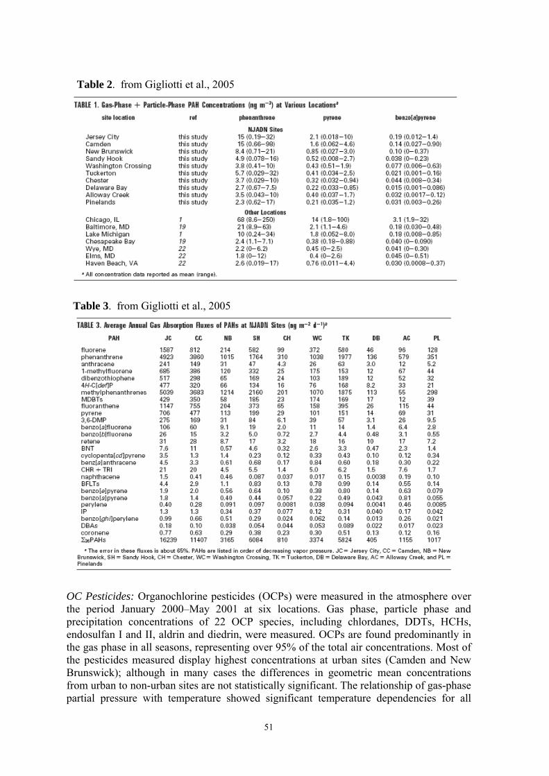
51

OC Pesticides: Organochlorine pesticides (OCPs) were measured in the atmosphere over the period January 2000–May 2001 at six locations. Gas phase, particle phase and precipitation concentrations of 22 OCP species, including chlordanes, DDTs, HCHs, endosulfan I and II, aldrin and diedrin, were measured. OCPs are found predominantly in the gas phase in all seasons, representing over 95% of the total air concentrations. Most of the pesticides measured display highest concentrations at urban sites (Camden and New Brunswick); although in many cases the differences in geometric mean concentrations from urban to non-urban sites are not statistically significant. The relationship of gas-phase partial pressure with temperature showed significant temperature dependencies for all

Table 3. from Gigliotti et al., 2005

Table 2. from Gigliotti et al., 2005

52

OCPs, except aldrin (i.e., decreasing concentrations with decreasing temperature). Atmospheric depositional fluxes (gas absorption into water +dry particle deposition + wet deposition) to the Hudson River Estuary of selected OCPs were estimated. Atmospheric concentrations of dieldrin, aldrin and the HCHs are similar to those measured by the Integrated Atmospheric Deposition Network (IADN) in the Great Lake Region. In contrast, concentrations of DDTs, chlordanes and heptachlor are higher in the Mid-Atlantic compared to the Great Lakes, suggesting a mix of local sources (recycling) and long range transport from the southern US and beyond.

Table 4. from Gioia et al., 2005

Table 5. from Gioia et al., 2005

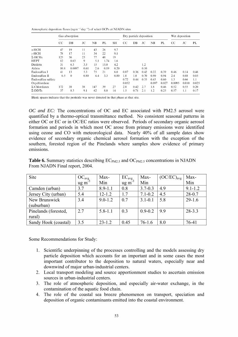
53

OC and EC: The concentrations of OC and EC associated with PM2.5 aerosol were quantified by a thermo-optical transmittance method. No consistent seasonal patterns in either OC or EC or in OC/EC ratios were observed. Periods of secondary organic aerosol formation and periods in which most OC arose from primary emissions were identified using ozone and CO with meteorological data. Nearly 40% of all sample dates show evidence of secondary organic chemical aerosol formation with the exception of the southern, forested region of the Pinelands where samples show evidence of primary emissions. Table 6. Summary statistics describing ECPM2.5 and OCPM2.5 concentrations in NJADN From NJADN Final report, 2004. Site OCavg

ug m-3 Max-Min

ECavg ug m-3

Max-Min

(OC/EC)avg Max-Min

Camden (urban) 3.7 8.9-1.1 0.8 3.7-0.3 4.9 9.1-1.2 Jersey City (urban) 5.4 12-1.2 1.7 7.1-0.2 4.5 28-0.7 New Brunswick (suburban)

3.4 9.0-1.2 0.7 3.1-0.1 5.8 29-1.6

Pinelands (forested, rural)

2.7 5.8-1.1 0.3 0.9-0.2 9.9 28-3.3

Sandy Hook (coastal) 3.5 23-1.2 0.45 76-1.6 8.0 76-41 Some Recommendations for Study:

1. Scientific underpinning of the processes controlling and the models assessing dry particle deposition which accounts for an important and in some cases the most important contributor to the deposition to natural waters, especially near and downwind of major urban-industrial centers.

2. Local transport modeling and source apportionment studies to ascertain emission sources in urban-industrial centers.

3. The role of atmospheric deposition, and especially air-water exchange, in the contamination of the aquatic food chain.

4. The role of the coastal sea breeze phenomenon on transport, speciation and deposition of organic contaminants emitted into the coastal environment.

54

5. Improved methodologies to assess magnitude of air – water exchange of organic compounds.

6. Focused studies on the evaluation of watershed retention of organic contaminants, especially of atmospheric origin.

7. Source apportionment of atmospheric organic compounds to evaluate sources to air, and sources to water.

8. Role of deposition versus atmospheric reactions in the removal of atmospheric organic compounds.

NJADN References Brunciak P. A., J. Dachs, T. P. Franz, C. L. Gigliotti, E. D. Nelson, B. J. Turpin, and S. J. Eisenreich. Polychlorinated Biphenyls and Particulate Organic/Elemental Carbon in the Chesapeake Bay Atmosphere. Atmos. Environ., 2001, 35, 5663-5677. Dachs, J., R. Lohmann, W. A. Ockenden, L. Méjanelle, S. J. Eisenreich and K.C. Jones. Oceanic biogeochemical controls on global dynamics of persistent organic pollutants. Environ. Sci. Tech, 2002, 36 (20), 4229 –4237. Dachs, J.; T. R. Glenn; C. L. Gigliotti; P. Brunciak; E. D. Nelson; T. P. Franz; S. J. Eisenreich. Occurrence and diurnal variability of PAHs in the Baltimore and adjacent Chesapeake Bay atmosphere. Atmos. Environ., 2002, 36/14, 2281-2295. Dachs, J.; S.J. Eisenreich. Adsorption Onto Aerosol Soot Carbon Dominates Gas-Particle Partitioning of PAHs. Environ. Sci. Tech., 2000, 34, 3690-3697. Dachs, J.; S.J. Eisenreich; J.E. Baker; F.-C. Ko; J.D. Jeremiason. Coupling of phytoplankton uptake and air-water exchange of persistent organic pollutants. Environ. Sci. Tech., 1999, 33(20), 3653-3660. Dachs, J.; S.J. Eisenreich; R.M. Hoff. Influence of eutrophication on air-water exchange, vertical fluxes and phytoplankton concentrations of POPs. Environ. Sci. Tech. 2000, 34(6), 1095-1102. Eisenreich, S.J.; P.A. Brunciak; J. Dachs; T. Glenn; C. Lavorgna; E.D. Nelson; L.A. Totten; D. Van Ry. "Persistent organic pollutants in the coastal atmosphere of the Mid-Atlantic states - USA. In Persistent Bioaccumlative Toxic Chemicals: I. Fate and Exposure, R. Lipnick, J.L.M. Hermens, K.C. Jones, D. Muir (Eds.), ACS Symposium Book Series # 772: Washington, D.C., 2000, 28-57 Gigliotti, C.; J. Dachs; E.D. Nelson; P.C. Brunciak; S.J. Eisenreich. Temporal and Spatial Trends of Polycyclic Aromatic Hydrocarbons in the New Jersey/Hudson River Estuary Coastal Atmosphere. Environ. Sci. Tech., 2000, 34, 3547-3554. Gigliotti, C.L. ; Totten, L.A.;. J. H. Offenberg, Jordi Dachs, J. R. Reinfelder, E. Nelson, T. R. Glen IV, S. J. Eisenreich. Atmospheric Concentrations and Deposition of PAHs to the Hudson River Estuary. Environ. Sci. Tech., 2005. 39, 5550-5559. Gigliotti, C.L.; Totten, L.; Brunciak, P.A.; J. Dachs; E.D. Nelson; R. Lohmann; S.J. Eisenreich.. Air-Water Exchange of PAHs in the NY-NJ Harbor Estuary. Environ. Toxic. Chem., 2002, 21, No. 2, 235–244. Gioia, R., J.H. Offenberg, C.L. Gigliotti, L.A. Totten, S.Du, and S.J. Eisenreich. Atmospheric concentrations and fluxes of organochlorine pesticides in the US Mid-Atlantic region. Atmospheric. Environment, 2005. 39, 2309-2322. Koelliker, Y.; L. A. Totten; C. L. Gigliotti; H. Offenberg; J. R. Reinfelder; Y. Zhang; S. J.

55

Eisenreich. Water, Air and Soil Poll. Atmospheric wet deposition of total phosphorus in New Jersey. Water, Air and Soil Pollution, 2004, 154: 139–150. Lee, C.H.; C.L. Gigliotti, J. H. Offenberg, S. J. Eisenreich; B. J. Turpin. Sources of polycyclic aromatic hydrocarbons to the Hudson River Airshed. Atmos. Environment. 2004, 38 (2004) 5971–5981. Lohmann, R., P.A. Brunciak, J. Dachs, C. L. Gigliotti, Eric Nelson, D. Van Ry2, T. Glenn, S. J. Eisenreich, J. L. Jones and K. C. Jones. Processes controlling duirnal variations of PCDD/Fs in the New Jersey coastal atmosphere. Atmos Environ., 2003, 37, 959-969. Lohmann, R.; E.D Nelson; S.J. Eisenreich.; K.C. Jones. Evidence for dynamic air - water exchange of PCDD/Fs: A Study in the Raritan Bay/Hudson River Estuary, USA. Environ. Sci. Tech.,34, 2000, 34(15); 3086-3093. Nelson E.D.;. S.J. Eisenreich Trends and dynamics of chlordanes in the coastal atmosphere of the Mid-Atlantic United States. Organohalogen Compounds, 1999, 41, 391-394. Offenberg, J.H.; E. D. Nelson, C. L. Gigliotti, S. J. Eisenreich. Chlordanes in Mid-Atlantic Atmosphere: NJADN 1997- 1999, Environ. Sci. Tech., 2004. 38, 3488-3497. Reinfedler, J.; L. Totten; S.J. Eisenreich. The New Jersey Atmopsheric Atmospheric Deposition Network. Final Rpt. To the NJ Department of Environmental Protection. 2004, 174 pp. Totten, L.A., G. Stenchikov, C. L. Gigliotti, N. Lahoti, S. J. Eisenreich. Measurement and Modeling of Urban Atmospheric PCB Concentrations On A Small (8 Km) Spatial Scale. Atmospheric Environment, 2005, In review. Totten, L.A.; C. L. Gigliotti, D. A. VanRy, J. H. Offenberg, E. D. Nelson; Dachs, J. R. Reinfelder, and S. J. Eisenreich. Atmospheric Concentrations and Deposition of PCBs to the Hudson River Estuary. Environ. Sci. Tech., 2004, 38, 2568-2573. Totten, L.A.; P. A. Brunciak; C. L. Gigliotti; J. Dachs; T. R. Glenn; E.D. Nelson; S.J. Eisenreich. Dynamic Air-Water Exchange of Polychlorinated Biphenyls in the New York-New Jersey Harbor Estuary. Environ. Sci. Technol., 2001. 35 (19), 3834 -3840, 2001. Totten, L.A.; S.J. Eisenreich Evidence for OH Radical Attack on PCBs During Tropospheric Transport. Organohalogen Compounds, 1999, 43, 353-357. Totten, L.A.; S.J. Eisenreich; P. C. Brunciak. Evidence For Destruction of PCBs by OH Radical In Urban Atmospheres. Chemosphere., 2002, 47, 735–746. Van Ry, D. A.; C. L. Gigliotti; T. R. Glenn; IV, E. D. Nelson; L. A. Totten; S. J. Eisenreich. Wet deposition of polychlorinated biphenyls in urban and background areas of the Mid-Atlantic States. Environ. Sci. Tech, 2002, 36(15); 3201-3209. Van Ry, D. A.; Dachs, J.; Gigliotti, C. L.; Brunciak, P.; Nelson, E. D.and S.J. Eisenreich. Atmospheric seasonal trends and environmental fate of alkylphenols in the lower Hudson River Estuary. Environ. Sci. Tech.,2000, 34 (12), 2410 -2417. Yan, S; J. Dachs, C-W. Fan, J. Reinfelder, S. J. Eisenreich. Air-Water Exchange Controls Phytoplankton Concentrations of Polychlorinated Biphenyls in Impacted Estuaries. Environ. Sci. Tech., 2005. In Review

56

ATMOSPHERIC DEPOSITION OF PERSISTENT ORGANIC POLLUTANTS TO THE OCEANS; INFLUENCE OF SPATIO-TEMPORAL VARIABILITY OF DEPOSITIONAL FLUXES ON ATMOSPHERIC RESIDENCE TIMES AND

LONG RANGE TRANSPORT.

Jordi Dachs1, Elena Jurado1, Steven J. Eisenreich2 and Kevin Jones2

1 Department of Environmental Chemistry. IIQAB-CSIC, Barcelona, Catalunya, Spain.

2 Joint Research Centre, Ispra, Italy. 3 Department of Environmental Science. Lancaster University, Lancaster, UK.

Wet and dry deposition fluxes of polychlorinated biphenyls and polychlorinated dibenzo-p-dioxins and furans to the European seas and global Ocean have been estimated by combining meteorological satellite data and measured atmospheric field concentrations. They are then compared to other atmospheric depositional mechanisms on the European and global scale. The atmospheric deposition fluxes are estimated with state of the art methods including contaminant adsorption onto raindrops and enhancement of dry gaseous diffusive fluxes due to the turbulence caused by the rain. Both, wet and dry deposition estimates show a high spatial and seasonal variability, with maxima located in the Intertropical Convergence Zone (ITCZ) and in low temperature regions for the wet deposition fluxes, and in high productivity regions for the absorption fluxes. For example, average wet deposition fluxes estimated for the Atlantic Ocean in this study are 110 ng m-2 y-1 and 45 ng m-2 y-1 for ΣPCB and ΣPCDD/Fs, respectively, one order of magnitude lower than net air-water diffusive exchange. Model validation using available coastal data measurements shows good agreement that falls within a factor of 2-3 in most cases. In the present paper, in addition to give the deposition estimates for the European seas, an assessment of the influence of the important spatial and temporal variability on atmospheric transport and residence times is given.

57

MASS BUDGET AND DYNAMICS OF POLYCHLORINATED BIPHENYLS IN THE EASTERN MEDITERRANEAN SEA

Manolis Mandalakis, Maria Apostolaki and Euripides G. Stephanou

Environmental Chemical Processes Laboratory (ECPL), Department of Chemistry,

University of Crete, GR-71409 Heraklion, Greece Introduction Even though the production of polychlorinated biphenyls (PCBs) was banned two decades ago, they are still released into the atmosphere by primary and secondary emission sources. Atmospheric PCBs tend to partition between the gas and particulate phase of the atmosphere1 and they are transported away from the release sources through the movement of air masses. Several studies have shown that atmospheric transport and deposition is a major mechanism by which PCBs and other semi-volatile organic compounds may enter the aquatic ecosystems2 and contribute to biota contamination. In the aquatic environment, these compounds can be dissolved in the water phase or associated with particles depending on their hydrophobicity and organic carbon-water partition coefficients. Particle-bound PCBs are subsequently removed from the water column by vertical transport of sinking particles3. The objectives of the current study, were i) to assess the dry particle deposition and the settling flux of PCBs in the atmosphere and the water column of the eastern Mediterranean, respectively and ii) to synthesize the results of the present and previous studies in order to construct a mass balance which will describe the behavior of PCBs in this region. Materials and Methods Particle dry deposition samples (twelve samples) for PCB analysis were collected from the marine background sampling station of Finokalia (35o 20' N, 25o 40' E; Island of Crete, Greece) between April 2000 and October 2001. Samples were collected by using a stainless steel funnel (42 cm of diameter) connected directly to an amber glass bottle. Prior to sampling, both the funnel and the bottle were thoroughly rinsed with HPLC quality grade acetone and then with Milli-Q water. Settling particles within the water column were sampled from May to October 2001. Sediments traps were deployed at three different depths (186, 1426, 2837 m) in southern Ionian Sea (35o 10' N, 20o 51' E). Fifty-four PCB congeners (corresponding to 41 chromatographic peaks) were quantified during this study. More information about the analysis and detection of PCBs has been reported in previous studies4.

Results and Discussion For all three sediment traps, the total mass flux exhibited a clear seasonal variation with the maximum values occurring during spring and summer and the lowest ones during autumn and winter months. At the upper sediment trap (186 m water depth), the mass flux ranged between 8 and 220 mg m-2 day-1, with an average value of 48 ± 65 mg m-2 day-1. Although similar values were observed at 1426 (4 to 300 mg m-2 day-1) and 2837 m water depth (6 to 259 mg m-2 day-1), the flux at the upper sediment trap was relatively higher throughout the spring. The concentration of ΣPCB in settling solids varied between 3.3 and 19.0 ng g-1 (dry weight; dw) with an average value of 7.0 ± 5.5 ng g-1 dw. For all sediment traps, the levels of PCBs were generally higher during summer than spring samples. Congeners 18, 8+5,

58

28, 31 and 20+33 were the most abundant and the concentration of each one ranged between 0.2 and 1.8 ng g-1 dw. For both sampling periods and especially during summer, the concentration of PCBs exhibited a decline with depth in the water column. In particular, the concentration of ΣPCB at the upper sediment trap ranged from 5.0 to 19.0 ng g-1 dw and it was substantially higher than those observed at the middle (4.5 to 7.4 ng g-1 dw) and near-bottom sediment trap (3.3 to 5.8 ng g-1 dw). For all depths, tetra- and tri-chlorinated congeners dominated the PCB pattern and accounted for 38 ± 5% and 22% ± 5% of the total PCB, respectively. For all traps deployed, the derived depositional flux of ΣPCB varied between 0.18 and 1.04 ng m-2 day-

1, with the upper and near-bottom sediment traps providing the highest and the lowest values, respectively. The arithmetic average flux of PCBs was 0.63 ± 0.34 ng m-2 day-1, while the corresponding time-weighted average flux approached 0.45 ng m-2 day-1. The estimated annual settling flux of PCBs below the euphotic zone (186 m water depth) approached 214 ng m-2 yr-1, while the corresponding fluxes at 1426 and 2837 m were 87 and 81 ng m-2 yr-1, respectively. By taking into account the surface area of the eastern Mediterranean Sea (1.65 million km2), it was roughly estimated that the annual load of PCBs under the euphotic zone should be around 350 kg, while only 40% of that amount (about 135 kg) will finally reach deeper waters. The dry deposition flux of PCBs was determined for each one of the twelve sampling periods. The flux of ΣPCB ranged from 0.1 to 1.1 ng m-2 day-1 with an average value of 0.5 ± 0.3 ng m-2 day-1. In consistence with the sediment traps samples collected from southern Ionian Sea and analyzed in the current study, PCBs 28, 31, 18 and 33+20 were also the predominant congeners in dry deposition samples. Tri- plus tetra-chlorobiphenyls constituted 50 to 70% of the total PCB mass, while congeners having seven or eight chlorines provided the minimum contributions (about 2% each). The average pattern of PCB homologues in dry particle deposition was very well correlated (R2>0.97, p<0.001) with the corresponding pattern in the sediment traps and those previously observed in precipitation samples5 and the atmospheric particulate matter1. Wet deposition of PCBs is a process that has been poorly studied in the broader region of Mediterranean Sea. Recent results have been presented for the coastal background sampling station of Finokalia in the eastern part of the Mediterranean5. The concentration of ΣPCB in precipitation samples (particles plus dissolved phase) collected from Finokalia ranged between 1.0 and 3.6 ng l-1, with an average value of 1.9 ± 0.9 ng l-1. The volume-weighted mean (VWM) concentration of ΣPCB was 1.8 ± 0.4 ng l-1. Tri- plus tetrachlorinated congeners accounted for 61% of total PCBs measured in rainwater, while the sum of hepta- and octachlorinated biphenyls accounted for less than 10%. Based on the precipitation rate and the VWM concentration of PCBs in rainwater the estimated annual wet deposition flux of PCBs should approach 820 ng m-2 yr-1. By taking into account the total surface area of eastern Mediterranean basin, the total load of PCBs in this area should be ca. 1.3 t yr-1. Diffusive gas exchange across the air-sea interface (volatilization/absorption) has been recognized as an import process for the delivery or the removal of PCBs from natural waters. In order to estimate the net vapor flux of PCBs (volatilization minus absorption) in the eastern Mediterranean Sea a modified two-film, gas exchange model was applied7. The atmospheric concentrations of gaseous PCBs have been monitored at the sampling station of Finokalia and these results have been previously reported1. The presence of PCBs in seawater of the Mediterranean basin has also been investigated6. The average values calculated from these results were subsequently used in our model. The concentrations of individual PCBs in the gas phase provided a significant correlation with the corresponding

59

concentrations in the dissolved phase of seawaters (R2=0.63, p<0.001). The fluxes of all individual congeners were positive (net volatilization) and ranged from +0.5 to +157 ng m-

2 yr-1. By summing up the fluxes of the congeners (18 chromatographic peaks) whose concentrations were available in both seawater and air, the flux of PCBs was +940 ng m-2 yr-1. Since, these congeners normally account for about 58% of ΣPCB (54 congeners) measured in different types of samples from the region of eastern Mediterranean (e.g. aerosols1, precipitation5, dry deposition and sediment trap samples, the gas-exchange flux of ΣPCB should approach +1600 ng m-2 yr-1. By considering the surface area of the eastern Mediterranean Sea, we estimated that the annual evaporation of PCBs should be 1550 to 3140 kg yr-1.

Based on laboratory-derived rate constants7, Anderson and Hites suggested that the reaction with OH radicals should be the major permanent loss process of PCBs from the atmosphere. Some field measurements provided evidence for the occurrence of this reaction under real tropospheric conditions8. In the present study, the destruction of PCBs was assessed for each of the four seasons by using a one-box approach. Our results showed that the destruction of total PCBs (54 congeners) should be about 8 times higher in the summer (3300 kg) than in the winter (400 kg), while similar amounts of PCBs should be destructed during spring (1700 kg) and fall (1250 kg). Regardless of the season, the congeners having 2 to 4 chlorines accounted for 86% of the total destruction, with trichlorinated congeners exhibiting the highest contribution (about 40%) to this process. The estimated annual destruction of PCBs in the atmosphere overlying the eastern Mediterranean Sea should approach 6650 kg yr-1 and this loss process is remarkably higher than the corresponding fluxes of dry and wet deposition. The potential losses from particles were predicted based on the volatility of individual PCB congeners9 and the concentrations in the gas-phase were back-corrected. Even after that adjustment, the calculated OH sink of total PCBs remained consistently high (6300 kg yr-1), though lower than our initial estimate. The mass balance is completed by assembling all of the fluxes estimated in the previously. The estimated pools of all PCBs in the atmosphere were clearly much lower than those in surface seawaters, and that was especially evident for the more chlorinated congeners. The atmospheric burden of ΣPCB approached 160 kg, while the corresponding burden in the euphotic zone should range between 46 and 84 t. Particle-bound PCBs accounted for only 1% of the atmospheric pool, though about 97% of these chemicals in the euphotic zone should be associated with suspended particles. The atmospheric input of PCBs in the eastern Mediterranean Sea through dry and wet deposition was estimated to be 0.3 and 1.3 t yr-1, respectively. The total atmospheric input estimated in the present study (1.6 t yr-1) is about 8 times lower that the input previously reported for the western part of the Mediterranean (24 t yr-1)2. The volatilization flux of ΣPCB from the eastern Mediterranean Sea due to air-sea exchange should be between 1.5 and 3.1 t yr-1 and overall it should offset the input from wet and dry deposition (1.3 plus 0.3 t yr-1). By considering the upper limit of this flux, it is more likely that, overall, the eastern Mediterranean Sea acts as a net source of PCBs to the atmosphere (volatilization minus wet and dry deposition) mainly due to the higher evaporation fluxes of the less chlorinated congeners (such as PCB 18 and 52). However, the opposite situation was apparent for some individual congeners such as PCB 28, 70, 110 and 180, whose evaporation fluxes were relatively lower than their inputs through atmospheric deposition. In addition, PCBs are removed from the euphotic zone with a settling flux of 350 kg yr-1. Assuming steady-state conditions for the surface waters, an additional inflow of PCBs should be required. The discharge of urban and industrial sewage, riverine input and the transport of more polluted surface waters from western to

60

eastern Mediterranean could justify such an inflow. The estimated destruction of ΣPCB by OH radicals (6.6 t yr-1) was approximately four times higher than the export flux due to atmospheric deposition (wet plus dry deposition). By subtracting inflows (volatilization) from outflows (destruction and deposition), a net decrease of 5.1 to 6.7 t yr-1 is predicted for ΣPCB, implying that the whole burden of these chemicals should be vanished from the atmosphere in 9 to 11 days. It was demonstrated that the destruction by OH radicals is of major importance for the fate of PCBs in this region but further research effort is required to better understand and evaluate the precise magnitude of this loss process. In addition, our calculations for the air-sea exchange of PCBs indicated that this process may also play an important role. More accurate estimates for the air-sea exchange flux of PCBs should further improve our knowledge regarding the mobility of these contaminants between the atmospheric and aquatic compartments.

Acknowledgments The Ministry of Education of Greece (EPEAEK Program) is acknowledged for financial support. References 1. Mandalakis M. and Stephanou E. G. (2002) J. Geophys. Res. 107: doi:10.1029/2001JD001566. 2. Tolosa I., Readman J. W., Fowler S. W., Villeneuve J. P., Dachs J., Bayona J. M. and

Albaiges J. (1997) Deep-Sea Res. II 44: 907–928. 3. Dachs, J., R. Lohmann, W. A. Ockenden, L. Méjanelle, S. J. Eisenreich, and K. C. Jones (2002)

Environ. Sci. Technol. 36: 4229-4237. 4. Mandalakis, M., Tsapakis M. and Stephanou E. G. (2001) J. Chromatogr. A 925: 183–196. 5. Mandalakis, M., and Stephanou E. G. (2004) Environ. Sci. Technol. 38: 3011–3018. 6. Schulz-Bull D. E., Petrick G., Johannsen H. and J. C. Duinker (1997) Croat. Chem. Acta 70:

309–321. 7. Anderson P. and Hites R. (1996), Environ. Sci. Technol. 30: 1756–1763. 8. Mandalakis M., Berresheim H. and Stephanou E. G. (2003) Environ. Sci. Technol. 37: 542–547. 9. Mandalakis M. and Stephanou E. G. (2002) Environ. Toxicol. Chem. 21: 2270–2275.

61

SOME THOUGHTS ON MEASURING ATMOSPHERIC DEPOSITION OF POPs

Michael S. McLachlan

Department of Applied Environmental Science, Stockholm University, Sweden

Introduction

Atmospheric deposition is a key vector for many POPs entering terrestrial and aquatic ecosystems. Consequently, it is valuable to be able to measure the atmospheric deposition of POPs to different surfaces. Over the past decades researchers have invested considerable effort in this challenge. This paper offers some perspectives on the capabilities and limitations of available methods based largely on the author’s experience.

Forms of Atmospheric Deposition

POPs can be deposited to surfaces in 4 physical forms: dissolved in a liquid, sorbed in a solid, adsorbed to a surface, or as a gas.

Deposition of dissolved chemical occurs in rain, whereby chemical in the atmosphere dissolves in raindrops and is advected to the receptor surface. This process depends on the POP levels in the atmosphere, the partitioning coefficient between rainwater and the gas phase, and the precipitation rate.

Many POPs sorb in atmospheric aerosols. POPs sorbed in this way are deposited when the aerosols are deposited. This can occur in two ways, either wet through scavenging of aerosols by rain or snow, or dry. Wet deposition via particle scavenging depends on the cloud dynamics (in cloud scavenging, fall height, droplet size, precipitation rate) as well as the particle size distribution of the aerosol-bound POPs. There are 3 mechanisms of dry deposition of atmospheric aerosols that depend largely on aerosol size: diffusion (small particles), impaction/interception (middle-size particles), and sedimentation (large particles). The magnitude of the dry deposition flux of the POPs depends on their particle size distribution as well as on micrometeorological conditions such as turbulence and, for the first two mechanisms, the surface properties.

POPs can also sorb to the surface of aerosols and be deposited with them. This mechanism becomes important when the specific surface area of the aerosol is high such as for snow or for fine fog droplets.

Gaseous deposition occurs when a POP molecule diffuses through the atmospheric boundary layer to a surface and is sorbed there. The inverse process, namely desorption of a molecule from a surface and diffusion through the boundary layer to the atmosphere, is called volatilization. The net gaseous exchange is the difference between the gaseous deposition and the volatilization. The direction of the net gaseous exchange is from the phase (i.e. surface or atmosphere) with higher chemical potential (or fugacity) to the phase in which it is lower. The rate of exchange can be described using Fick’s Law and is determined by the magnitude of the fugacity gradient, the surface area through which exchange is occurring, and mass transfer coefficients describing the resistance to diffusive transport in the different phases involved.

The relative importance of the different forms of deposition depends on the partitioning properties of the POP (1,2). A high particle/gas partition coefficient will increase the relative

62

importance of particle bound deposition, and a low Henry’s Law Constant will increase the relative importance of deposition of dissolved chemical. Identifying the principle deposition mechanism(s) is necessary in order to select appropriate methods for measuring atmospheric deposition.

Measuring Atmospheric Deposition

The following discussion focuses on the possibilities of measuring total atmospheric deposition. This challenge is assessed from the perspective of the different forms of deposition, but the discussion does not address issues of trying to separately quantify different forms of deposition.

a) Dissolved Chemical The atmospheric deposition of dissolved POPs is comparatively simple to quantify. It is a matter of collecting the rain and analyzing it for the chemical. The one fundamental problem that can arise is that it may be difficult to properly collect the vertical rain flux at exposed, windy locations. There are of course other issues of a general nature that pertain to sampling POPs, such as avoiding sample contamination, sorptive losses in the sampling system, and sample conservation. These challenges are in general quite manageable compared to some of the difficulties posed by other forms of deposition (see below).

b) Sorbed Chemical – Precipitation Scavenging of Aerosols Quantifying the atmospheric deposition of POPs associated with scavenged aerosols is comparable to sampling dissolved POPs (see above); one must simply collect the vertical flux of the precipitation and analyze it. One difference is that the aerosols will tend to stick to the surfaces of the samplers. Care must be taken to ensure that these aerosols are not lost again during the sampling period, that this part of the sample is also conserved adequately (e.g. the POPs are not subject to photodegradation on the surface of the sampler), and that the aerosols adhering to surfaces are included in the final sample that is extracted.

c) Sorbed Chemical – Dry Deposition The discussion of sampling dry deposition of aerosols must consider the mechanism of deposition. Deposition by sedimentation has similarities with precipitation scavenging of aerosols. In particular, the deposition flux is independent of the properties of the surface. This means that a surrogate surface such as a bulk deposition sampler can give a representative measure of the deposition flux to the surface. Note that problems with sample conservation can be larger, since large, dry aerosols are subject to blow out from samplers. However, these problems are manageable, at least under central European conditions. A study of the sampling artifacts associated with a glass bulk deposition sampler indicated that the loss of aerosol-associated PCDD/Fs from the sampler over a 1 month sampling period was negligible (3). Indeed, efforts to immediately conserve the sample led to other undesirable artifacts.

Dry deposition via impaction/interception and diffusion are, on the other hand, strongly dependent on the nature of the surface. This means that a surrogate surface is highly unlikely to give a good representation of the deposition flux by this mechanism, particularly over a wide range of environmental conditions. This poses a fundamental obstacle to measuring this component of the deposition flux of POPs.

Fortunately, measurements indicate that under conditions in central Europe this flux is not important. In a study of sampler characteristics it was found that >95 % of the bulk

63

deposition of PCDD/Fs was associated with wet deposition or dry sedimentation, while <5 % was associated with other mechanisms such as particle impaction/interception or diffusion (3). In another study, calculations of deposition rates based on measurements of the particle size distribution of PAHs and PCDD/Fs indicated that <20% would be associated with dry deposition of particles <4.05 μm (4). A third study showed that even for forest canopies, which are very effective at scavenging aerosols, dry deposition via these mechanisms accounted for just 40-60 % of the total deposition of 5-ring PAHs and higher chlorinated PCDD/Fs (5). Taken together, this is strong evidence that these forms of dry deposition need not be measured when assessing the atmospheric deposition of POPs in Europe, with the exception of forested ecosystems for which there are alternatives (see below). However, one should be aware there may be areas in Europe where factors such as a dry climate and remoteness from particle sources (i.e. comparatively few large aerosols in the atmosphere) converge to make these forms of deposition important.

d) Adsorbed Chemical Comparatively little is known about sampling the deposition of POPs adsorbed to surfaces. While fog is known to contain high levels of some POPs, many forms of fog do not deposit on surfaces, and quantifying the quantity that is deposited is difficult. Orographic fog is the one form that has the potential to be a meaningful deposition vector. Fog water is typically sampled by sucking air through a vertical or tilted screen where the fog droplets coalesce to larger drops and then run down the screen to be collected in a jar. This method has the potential for seriously underestimating the POP levels in the fog since the adsorptive surface area of the fog droplets is reduced by orders of magnitude while the exposure to air is very high, so that chemical volatilization during sampling is likely.

Deposition of chemical adsorbed to snow has been postulated to be an important form of deposition for some POPs in cold climates (6). However, the behavior of POPs in snow is just beginning to be explored, and there is little experience with sampling methods. Migration of chemical within the snow following deposition may have to be considered. In addition, it can be anticipated that any reduction of snow surface area during sampling will result in undersampling of the POPs. Consequently, careful sampling coupled with melting and extraction in sealed containers (7) is likely necessary.

e) Gaseous Chemical Gaseous deposition is the least tractable of the different forms of POP deposition, largely because it is dependent on surface properties in addition to chemical and meteorological properties, and because it is a bidirectional process. Different approaches are available to attempt to quantify this flux.

Perhaps the most common approach is to determine the diffusion gradient between the atmosphere and the surface phase, and to calculate the flux using an estimated mass transfer coefficient. The diffusion gradient is determined by measuring the concentrations in the two phases (e.g. the gaseous concentration in the atmosphere and the freely dissolved concentration in a water body) and then converting them into comparable units using equilibrium partition coefficients (e.g. the Henry’s Law Constant in the example above). This approach is fraught with challenges, which begin with developing sampling methods that permit separation of e.g. the gaseous and freely dissolved fractions from the total POP concentration in the atmosphere and the water body respectively. This sampling problematic and the difficulties of ultra-trace analysis of POPs in the environment result in measurements with a comparatively high level of uncertainty (typically >20%). To this comes the uncertainty in the equilibrium partition coefficient(s), which can be even larger.

64

This can lead to a fundamental problem, namely in calculating the difference between two uncertain numbers. If the diffusion gradient is very strong in one direction, i.e. if one of the two numbers (i.e. fugacities or chemical potentials) is much larger than the other, then a reasonable estimate of the gaseous exchange flux may be possible. However, if the numbers are similar (i.e. the system is close to a partitioning equilibrium), then their uncertainty may render it impossible to make statistically valid conclusions about the direction of the net gaseous exchange of the POP, let alone the flux (8).

A second major limitation of the diffusion gradient method lies in the limited temporal resolution in the measured POP concentration, a consequence of the costly sampling and analysis procedures. POP concentrations in the atmosphere vary widely on a time scale of hours or days, while sampling is often intermittent or integrates over periods of a week or even longer. Other variables in the mass transfer equation such as temperature, wind speed, or aerosol concentration also vary widely over short time scales, and in many cases these variables are correlated with the variation in atmospheric concentrations. If this variability is not taken into account and long-term averages are used instead, serious errors can result, particularly if the system is close to a partitioning equilibrium. For instance, even if the long term average air concentration indicates that a POP in an air/water system was at equilibrium (no net gaseous exchange), it could be that short periods of high atmospheric concentration of the POP coupled with low temperatures and high winds actually resulted in considerable gaseous deposition during this interval, and that this deposition was not compensated during the longer periods of low atmospheric concentrations, high temperatures, and low winds.

Another approach to measuring net gaseous exchange of POPs is to employ micrometeorological techniques. Eddy correlation techniques are used to measure fluxes of trace gases to and from surfaces. However, these techniques require the determination of POP concentrations in air with a high temporal resolution (hours or less) and a high precision. Due to the large volumes needed for POP analysis in air and the comparatively poor precision of the methods, this approach has not been widely pursued. In addition, the deposition fluxes cannot be readily extrapolated over large areas.

Relaxed eddy accumulation is an alternative technique, whereby a rapidly switching valve diverts air to one of two samplers, depending on whether the air package is moving up or down at that moment. This method has rapidly gained broad acceptance in measuring trace gas fluxes, but it has, to my knowledge, not yet been applied to POPs.

A third approach to measuring net atmospheric deposition of POPs including net gaseous exchange is to measure a flux or a change of inventory in the receptor phase. In the case of aquatic ecosystems, the sedimentation rate can be measured. However, as the enormous experience in study ocean carbon fluxes has shown, there are difficulties in quantifying sedimentation fluxes. In addition, knowledge of other possible contributors to the POP sedimentation flux such as non-atmospheric inputs of POPs or sediment resuspension is required. Nevertheless, this may be the only feasible approach for estimating atmospheric deposition in some cases, and it has an advantage in that it places the atmospheric flux in the context of the other fluxes affecting levels in the aquatic environment.

In the terrestrial environment, measuring the change of inventory in soils may be used to estimate net atmospheric deposition (sediments can conceivably be used in the aquatic environment in a similar way). However, this requires a good knowledge of loss processes in the soil (erosion, leaching, degradation, etc.). Furthermore, it can frequently only be

65

applied over long time scales due to the slow rates of change in the POP inventory and the limited precision of trace analytical methods for POPs.

Forested ecosystems offer an interesting alternative. There, gaseous deposition occurs mainly to the forest canopy. However, only a small fraction of the deposition is stored there for longer periods; the remainder is transported to the forest floor with leaf fall or via erosion of cuticle and bark particles. Hence gaseous deposition is essentially transformed into particulate deposition, which can be sampled using bulk deposition samplers as outlined above (5). Thus, sampling bulk deposition under forest canopies is perhaps the best method for long term monitoring of atmospheric deposition of semivolatile POPs, albeit with a time resolution of a year or more.

Summary

If a POP is deposited primarily in dissolved form, the flux can be quantified comparatively easily. The same is true if the deposited POPs are largely sorbed in aerosols, although more care must be taken. Problems may arise if the sorbed chemical is photochemically labile, or under unusual conditions in which dry deposition of small particles is the predominant mechanism. Little can be said at this point about chemicals that are primarily deposited when adsorbed to surfaces. For POPs that are deposited mainly as gases, fundamental problems still exist. Reasonable estimates of net gaseous exchange may be obtained if there is a strong thermodynamic disequilibrium between the atmosphere and the surface, but not if the system is close to equilibrium. Forest ecosystems are a notable exception, as the net gaseous deposition is captured in bulk deposition measurements below the canopy.

References

1. Mackay D., Paterson S., Schroeder W.H. (1986) Environ. Sci. Technol. 20: 810-816. 2. Lei Y.D., Wania F. (2004) Atmos. Environ. 38: 3557-3571. 3. Horstmann M., McLachlan M.S. (1997) Atmos. Environ. 31: 2977-2982. 4. Kaupp H., McLachlan M.S. (1999) Atmos. Environ. 33: 85-95. 5. Horstmann M., McLachlan M.S. (1998) Atmos. Environ. 32, 1799-1809. 6. Daly G., Wania F. (2004) Environ. Sci. Technol. 38: 4176-4186. 7. Gustafsson Ö., Andersson P., Axelman J., Bucheli T.D., Kömp P., McLachlan, M.S., Sobek

A., Thörngren J.-O. (2005) Sci. Total Environ. 342: 261-279. 8. Bruhn R., Lakaschus S., McLachlan M.S. (2003) Atmos. Environ. 37: 3445-3454.

66

MEASURING AND INTERPRETING POP AIR CONCENTRATION GRADIENTS ALONG ENVIRONMENTAL TRANSECTS

Frank Wania

University of Toronto at Scarborough, Department of Physical and Environmental

Sciences, 1265 Military Trail, Toronto, ON, Canada.

The development of novel passive air sampling techniques has made it possible to measure long term averaged air concentrations of persistent organic pollutants at numerous locations simultaneously, thus providing the capability for the mapping of the spatial variability of such concentrations. Using an XAD-based passive sampling technique we measured air concentration gradients of organochlorine pesticides and polychlorinated biphenyls along a number of environmental transects on the continental, national and regional scale. A focus of the latter is on elevation gradients under different climatic conditions. The recorded changes in the absolute POP concentrations, in the relative abundance of different POPs, and in the enantiomeric composition of chiral POPs, can be interpreted to yield information on (1) sources of POPs to the atmosphere, (2) the relative mobility and persistence of POPs in the atmosphere, and (3) the distribution and accumulation behaviour of POPs along environmental gradients. This interpretation is greatly facilitated if the air concentration measurements are paired with measurements of POPs in surface compartments and combined with multimedia fate model simulations. This will be illustrated using examples from North America, the Canadian Rocky Mountains and Costa Rica.

67

PASSIVE AIR SAMPLING FOR PERSISTENT ORGANIC POLLUTANTS: THE STATE OF THE ART

Kevin C. Jones (1), Tom Harner (2), Michael Bartkow (3), Ivan Holoubek (4), Jana Klanova (4), Frank Wania (5), Rosalinda Gioia (1), Claudia Moeckel (1), Andrew J.

Sweetman (1) and Gan Zhang (6)

(1) Environmental Science Department and Lancaster Environment Centre, Lancaster University, Lancaster, LA1 4YQ, United Kingdom

(2) Meteorological Service of Canada, Environment Canada, 4905 Dufferin Street, Toronto, Ontario, Canada M3H 5T4.

(3) National Research Centre for Environmental Toxicology (ENTOX), University of Queensland, Coopers Plains, Queensland, 4108, Australia.

(4) RECETOX - Research Centre for Environmental Chemistry and Ecotoxicology, Masaryk University, Kamenice 3/126, 625 00 Brno, Czech Republic

(5) Department of Physical and Environmental Sciences, University of Toronto at Scarborough, 1265 Military Trail, Toronto, Ontario, Canada, M1C 1A4.

(6) Guangzhou Institute of Geochemistry, Chinese Academy of Sciences, Guangzhou 510640, China.

The context – why develop passive air sampling techniques for POPs? ‘Persistent organic pollutants’ (POPs) is a generic term, encompassing many organic contaminant classes, including polynuclear aromatic hydrocarbons (PAHs), polychlorinated dibenzo-p-dioxins and –furans (PCDD/Fs), polychlorinated biphenyls (PCBs), and several other industrial and agricultural chemicals. Concerns about POPs centre around their persistence, bioaccumulation and sub-chronic toxicity potential, and propensity to undergo long-range atmospheric transport (LRAT). National and international controls on the production and use of POPs have been (or are being) introduced, notably through the Stockholm Convention (SC) administered with the UN Environment Programme (UNEP) and the LRTAP Protocol of the United Nations Economic Commission for Europe (UNECE). The role of the atmosphere in supplying POPs to terrestrial and aquatic foodchains, and in their global re-cycling is of key importance. This may follow emissions from obvious and strong point sources (e.g. PCDD/Fs from poorly operated incinerators), or from diffusive primary (e.g. PAHs from numerous combustion sources such as vehicles, domestic heating etc) and secondary sources (e.g. ‘old’ pesticides emitted from soils). This has focussed international regulation on reducing emissions to air (1, 2), and risk assessment/modelling efforts on their ambient distribution (3). Air monitoring for POPs has conventionally been conducted at a very limited number of sites using ‘active’ or high volume air samplers. These are expensive, require electricity and a trained operator. For example, in the United Kingdom, the Toxic Organics Micro-Pollutants (TOMPs) air monitoring network operated on behalf of the UK Department of the Environment, Food and Rural Affairs (Defra) uses only 6 such sites nationally, while other pollutants – such as NOx and ozone – are routinely sampled at tens-hundreds of locations nationally/regionally, using much cheaper sampling technologies, such as passive diffusion tubes. Regulatory and other developments mean there will be a pressing need to obtain more POPs data for air, in a much more routine and cost-effective way, to ensure compliance. This provides the incentive to develop new and cheaper passive air sampler (PAS) options.

68

Some major developments, driving the development of PAS for POPs are:

a. Under the SC, signatory countries must conduct source inventories, identify ongoing sources, and provide environmental monitoring evidence that ambient levels of POPs are declining. Developing countries, in particular, require cost effective and simple approaches that can operate in the absence of power. Generally, they lack the money to buy equipment (both sampling and analytical), to build the laboratories, to train their personnel, to finance the regular monitoring campaigns. PAS offer the opportunity to solve several of these problems, in the short-term. Such inexpensive and easy-to-handle devices also offer the option of shipping samplers and filters for exposure, and returning the filters for final analysis. In addition, a ‘Global Monitoring Network’ is being designed, with the objective of establishing baseline trends at global background sites (see 4, 5);

b. In the EU, an air quality standard is to be adopted for PAHs, because of health concerns over the carcinogenic properties of this compound class (6). There has been much discussion over the limit to be adopted, because of concerns over exceedances, even in rural areas where coal/wood are used for space heating, or near roadsides. Air quality standards for 1,4-butadiene have also been proposed, and limits for POPs may follow in the future. Once an air quality standard is adopted, there will be the requirement for local authorities to test for compliance.

c. Attention is focusing on occupational and indoor exposure to airborne POPs, because this can be an important source to workers and the general public. PAS can be used to unobtrusively sample indoor air, helping to identify sources/hotspots.

d. National Environment Agencies increasingly need to identify ‘less obvious’ diffusive sources of POPs, as they seek to further reduce emissions, now that more obvious primary sources have been/are becoming better controlled. PAS can be used to conduct ‘screening/reconnaissance surveys’, and are sensitive to site-/source-specific compound fingerprinting. They can therefore be used to help identify sources, and be used to help direct/target cost-effective active air sampling campaigns.

e. There is considerable interest in mapping the ambient distribution of POPs, to support national/international air monitoring networks, and to yield input data for regional distribution models. Studies have been conducted to demonstrate the feasibility of such ‘national’ or ‘continental scale’ measurement/modeling programmes, by preparing and supplying PAS to be deployed simultaneously across large areas – even at the continental and global scale (7-9). The samplers are then ‘harvested’, sealed and returned to the laboratory for analysis, data interpretation and modeling.

f. Besides their obvious usefulness for monitoring, mapping and source identification, PAS can also serve as tools in scientific investigations, by for example recording changes in atmospheric POP concentration and composition along environmental gradients (e.g. urban – rural; latitudinal; altitudinal; chiral signatures).

g. Passive air sampling techniques are particularly suited to complement and serve in the evaluation of compartmental multimedia fate and transport models, such as those exemplified by the fugacity approach (10). Like these models, PAS are specifically designed, and therefore most appropriate, for persistent organic

69

chemicals (11), and tend to provide information on the long term average conditions in the atmosphere and ignore variability on a shorter time scale. Passive samplers have not yet reached a stage of maturity, which would allow the measurement of volumetric air concentrations with an accuracy approaching that of pumped samplers. The progress towards quantitative calibration notwithstanding, the strength of PAS lies in their ability to provide compositional information, such as parent/metabolite ratios, chiral signatures (8, 9) and congener compositions of complex mixtures, such as the PCBs (12). As long as the chemicals being compared are not approaching equilibrium between sampler material and atmospheric gas phase, even changes in PAS uptake kinetics with wind speed - as has been observed for some sampler designs - will not affect the relative abundance of isomers, enantiomers and congeners. Incidentally, multimedia fate and transport models are also much better suited to predict compositional and relative information than absolute concentrations, because the latter depend on knowledge of the absolute emission rate, which for POPs is hardly ever known with high precision or accuracy (11).

What approaches can be used? As just indicated, there are considerable incentives to develop passive air sampling techniques. These should be simple to use, cheap, versatile and capable of being deployed in many locations concurrently. Passive samplers can be designed and calibrated, to allow reliable estimates of air concentrations to be made, or to allow semi-quantitative comparisons of the levels and patterns of POPs. Several designs are possible and – indeed – desirable. For example, it would be useful to have samplers to integrate ambient concentrations over time scales as short as hours/days or as long as weeks/months/years. The shorter timescales facilitate studies of contaminant dispersal, fluxes and transport processes and can provide data for dispersion/transport modeling. Longer timescales would allow source/sink regions to be identified and underlying trends in ambient levels to be investigated. Workers in the field have therefore been involved in development/deployment of a ‘suite’ of passive sampling designs and tools. The type, design and deployment can be varied. The principles behind PAS for POPs have been discussed in some detail elsewhere (e.g. 13, 14). However, in brief, gas phase compounds partition into the sampling medium during an uptake phase and – if the exposure time is long enough – approach equilibrium, which is in turn a function of temperature. Depending on the deployment conditions, the uptake rate may be affected by wind speed (i.e. air-side resistance can limit uptake rates). Samplers are therefore deployed in chambers to buffer the flow of air (to normalise uptake rates for PAS deployed in different locations and protect from compound photodegradation), and isotopically labeled (i.e. non-native) permeation reference compounds (PRCs) can be added to the PAS, so that loss (itself a function of wind speed) can be measured and used as a correction factor. Furthermore, the capacity and time to equilibrium can be varied by the choice of sampler type, storage medium and size. The total capacity of the sampler at equilibrium also differs between compounds; chemicals with higher equilibrium partition coefficients will take longer to reach equilibrium. For many POPs, the atmospheric burden is predominantly in the gas phase – in which case the general principles described above apply. However, some POPs are almost exclusively present on aerosols at ambient temperatures; this is a potential confounding factor since ultrafine particles (<100s nm) move through the atmosphere much like gases, and adhere

70

to/become trapped by the sampler. The theory of these issues has been addressed in our various publications and the necessary uptake and calibration studies performed against the conventional Hi-Vol active samplers. Sampling can therefore be conducted in the kinetic or equilibrium sampling mode, and – through knowledge of the uptake rates, equilibrium partition coefficients (and their temperature correction factors, and the ambient conditions - air concentrations can be derived/estimated from the measured mass of a given POP on the PAS. Future improvements and needs Often PAS are used in applications where information on the relative amounts or patterns of POPs is obtained, which can highlight spatial patterns and trends. This can be an extremely useful output and worthy goal. However, if PAS are to find favour as a ‘routine monitoring tool’, they will need to be used to derive an estimate of the ‘true’ air concentration, within a certain known tolerance, in a reproducible and sensitive way. Currently, PAS techniques are generally believed to enable estimates of the ‘true concentration’ within a factor of 2-3. Workers in the field are therefore currently focusing on:

a. better understanding sampler performance (e.g. reproducibility, robustness, ability to operate under different environmental conditions, calibration against active samplers);

b. better understanding of the influence of environmental variables (i.e. wind speed, temperature, humidity; influence of particle-bound POPs; photodegradation/ stability of compounds);

c. optimization of sampler design, deployment device/housing design, sample location/frequency etc.

d. best practice for preparation, pre-cleaning, PRC spiking amd loss correction, etc. Once these studies have reached fruition, clear recommendations can be given, to help those planning monitoring or research programmes, where passive sampling brings benefits. As we have seen in other fields, such as the now routine monitoring of gaseous pollutants with diffusion tubes, PAS can then be used widely and with confidence – to address the research, monitoring and regulatory challenges ahead. References 1. UNECE (1998) Protocol on Persistent Organic Pollutants under the 1979 Convention on

Long-Range Transboundary Air Pollution; United Nations Economic Commission for Europe (ECE/EB.Air/60).

2. UNEP (1998) Preparation of an Internationally Legally Binding Instrument for Implementing International Action on Certain Persistent Organic Pollutants; United Nations Environment Programme, UNEP/POPs/Inc.1/6.

3. Klecka, G., Boethling, B., Franklin, J., Graham, G., Grady, L., Howard, P., Kannan, K., Larson, R., Mackay, D., Muir, D. and van de Meent, K. (2000). Evaluation of persistence and long-range transport of organic chemicals in the environment. SETAC Special Publication Series. Pensacola, Fl., USA.

4. United Nations Environment Programme UNEP (2003). Proceedings UNEP Workshop to Develop a Global POPs Monitoring Programme to Support the Effectiveness Evaluation of the Stockholm Convention. Geneva, Switzerland, 24-27 March 2003.

5. Harner, T., Pozo Gallardo, K., Gouin, T., Macdonald, A-M., Hung, H., Cainey, J. and Peters, A. (2006). Global pilot study for persistent organic pollutants (POPs) using PUF disk passive air samplers. Environmental Pollution (in press).

71

6. European Commission (2001) Ambient air pollution by polycyclic aromatic hydrocarbons (PAH). Position paper; Luxembourg, Luxembourg.

7. Jaward, F. M., Farrar, N. J., Harner, T., Sweetman, A. J., Jones, K. C. (2004a) Passive air sampling of PCBs, PBDEs, and organochlorine pesticides across Europe. Environmental Science and Technology 38, 34-41.

8. Shen, L., Wania, F., Lei, Y.D., Teixeira, C., Muir, D.C.G. and Bidleman, T.F., 2005. Atmospheric distribution and long-range transport behaviour of organochlorine pesticides in North America. Environmental Science and Technology 39, 409-420.

9. Shen, L., Wania, F., Lei, Y.D., Teixeira, C., Muir, D.C.G., and Bidleman, T.F. (2004) Hexachlorocyclohexanes in the North American atmosphere. Environmental Science and Technology 38, 965-975.

10. Mackay, D. (2001). Multimedia Environmental Models: The Fugacity Approach. Chelsea, MI: Lewis Publishers.

11. Wania, F. and Mackay, D. (1999). The evolution of mass balance models of persistent organic pollutant fate in the environment. Environmental Pollution 100, 223-240.

12. Ockenden, W. A., Sweetman, A., Prest, H. F., Steinnes, E. and Jones, K. C. (1998). Toward an understanding of the global atmospheric distribution of persistent organic pollutants: the use of semi-permeable membrane devices as time integrated passive samplers. Environ. Sci. Technol. 32: 2795-2803.

13. Ockenden, W. A., Jaward, F. M. and Jones, K. C. (2001). Atmospheric sampling of persistent organic pollutants: needs, applications and advances in passive air sampling techniques. TheScientificWorld, 1, 557-575.

14. Shoeib, M., Harner, T. (2002) Characterisation and comparison of three passive air samplers for persistent organic pollutants. Environment Science and Technology, 36, 4142-4151.

72

TRACING ATMOSPHERIC DEPOSITION OF POPs IN AQUATIC SYSTEMS: LAKE MAGGIORE CASE STUDY. FIRST RESULTS ON PCDD/Fs.

J. Castro-Jiménez1, E. Canuti1, E.H. Christoph1, S.J. Eisenreich2, G. Hanke1, G. Mariani1

H. Skejo1, and G. Umlauf1

1 Institute for Environment and Sustainability, TP 290. 2 Institute for Health and Consumer

Protection, TP 582. European Commission, Ispra, Italy 21020. Introduction Polychlorinated dibenzo-p-dioxins and dibenzofurans (PCDD/ Fs) enter the environment primarily as a result of anthropogenic activities. Many of the congeners bioaccumulate and are considered potent toxicants capable of producing a wide spectrum of adverse health effects in biota and humans such as immunotoxicity, chloracne, carcinogenicity, reproductive and developmental toxicity, disruption of the endocrine system, induction of enzymes, and anti-estrogenic effects1. As a chemical class, they occur as byproducts of chemical manufacturing and incineration processes1-3. Emissions from incineration of medical, municipal, and chemical wastes and certain facilities in central Europe4 provide the major source of PCDD/F to the environment. PCDD/Fs are delivered to lake systems by atmospheric emission and transport followed by deposition, direct and indirect discharges, and riverine inputs. Polychlorinated dioxins and furans (PCDD/Fs) for example are characterized by low aqueous solubilities and vapor pressures, and resistance to extensive chemical and biological transformation. Their general hydrophobic nature results in high partition coefficients to abiotic and biotic particles. PCDD/Fs exist in the atmosphere as gases and particles although most measurements are dominated by the aerosol concentrations, especially the black carbon (BC) fraction. Once delivered to the water column, the primary removal processes are adsorption to or partitioning into particles and subsequent settling and accumulation in bottom sediments. The sorptive properties are largely controlled by the organic carbon (OC) content of particles, although BC may also play a role. Thus hydrophobic organic contaminants (HOCs) will follow the path of the average clay-size particles and be focused into the more quiescent, depositional basins of the lake. Experience from the Laurentian Great Lakes shows that residence times for HOCs are about 2-4 times the fine-particle residence times of ~ 1 year. Once delivered to the bottom sediments, contaminant and particle burial is slowed by the effects of resuspension and mixing of surface sediments by aquatic organisms. Several studies have focused on the atmospheric transport, reactivity and deposition of these compounds but relatively few on their in-lake behavior. In this work, we provide preliminary information on the delivery and accumulation of PCDD/Fs as recorded in sediments from the Lake Maggiore (LM), the second largest lake in Italy (Figure 1).

73

Our strategy was to obtain surface sediment from areas near riverine inputs and in the depositional basins, settling material in sediment traps at one site and preliminary air, aerosol and rain profiles. Similarity in isomer profiles in atmospheric aerosol, rain, water column settling matter and bottom sediment point to an important if not dominant contribution from atmospheric deposition to LM, especially derived from aerosol-bound PCDD/Fs. Later high resolution sediment cores will be analyzed to provide a spatial and temporal view of organic contaminant loading to the lake. Materials and Methods Sampling Sediment (bottom and settling material), air and precipitation samples were taken in the LM area. Sampling locations are depicted in Figure 2. Ambient air: The air sample was taken at the Joint Research Centre (JRC) EMEP Ispra Site5. A weekly sample was collected using a high volume sampler (Echo PUF Hi volume sampler, TCR Tecora, Milano, Italy). A total volume of 845 Nm3 was obtained. Previously cleaned glass fiber filter (GFF) of 102 mm diameter and polyurethane foam (PUF) of 65 mm diameter and 75 mm length were used for the retention of the studied compounds.

Location 194 m above s.lLength 66 km (IT +SZ)Width max. 10 kmWidth med. 3.9 kmArea 212.5 km²Volume 37.5 km³Coastline 170 kmMax. depth 370 mMedium depth 176 m

Location 194 m above s.lLength 66 km (IT +SZ)Width max. 10 kmWidth med. 3.9 kmArea 212.5 km²Volume 37.5 km³Coastline 170 kmMax. depth 370 mMedium depth 176 m

Figure 1. Lake Maggiore (Northern Italy)

74

Particulate phase (filter) and gas phase (PUF) were analyzed separated. PM10 data were also obtained from the JRC EMEP Ispra Site. Wet deposition: A device holding three glass funnels of 188 mm diameter each was used for the precipitation collection. A PUF of 18 mm diameter and 100 mm length was placed in each neck funnel. Precipitation was estimated by gravimetric method. Sediment sampling: Sediment surface grab samples where taken with a Ponar Grab sampler from a boat in the estuary zone of rivers flowing into LM and in the area of the deployed sediment trap. The sampled sediment depth was 5 – 10 cm. Supernatant water was decanted, sediment was frozen and freeze dried (Lio5P, 5 Pascal, Trezzano, Italy). Material > 2 mm was removed by sieving. Sample storage at – 30 °C. An amount of 40 g was processed. Sampling of settling material: The sediment trap (JRC central workshop), stainless steel, diameter 50 cm, 150 cm cylinder with funnel end and 250 ml glass sample container, was deployed at 30 m water depth, 3 m above the sediment, using an acoustic release unit 7986 LRT (Sonardyne, Yateley, UK). The trap was deployed on 17 Dec 04 and recovered on 19 April 05. Sample dry weight was 15.75 g. The sample was centrifuged, frozen, freeze dried and stored at – 30 °C until extraction. An amount of 5 g was processed. Analytical determinations: Samples were extracted with n-hexane/acetone (220/30) by soxhlet for 48 h after spiking with internal standards (16 13C-labelled 2,3,7,8-chlorine-substituited congeners- 400 pg each, except OCDD/OCDF with 800 pg each). Extract purification was executed with an automated clean-up system (Power-Prep P6, from Fluid Management Systems (FMS) Inc., Watertown, MA, USA) after treatment with conc. H2SO4 (the latter was done only for sediments and settling material). Analysis of PCDD/Fs was based on isotope dilution using HRGC-HRMS (high resolution gas chromatography – high resolution mass spectrometry) for quantification. The GC (HP-6890, Hewlett Packard, Waldbronn, Germany), was coupled with a VG Autospec Ultima mass spectrometer (Micromass, Manchester, UK) operating in EI-mode at 34 eV with a resolution of >10000. The samples were analyzed on a 60 m capillary column with 0.25 mm i.d. and 0.25 µm film (BP-DXN, SGE, Victoria, Australia). The applied methodology follows USEPA method 16136. For QA/QC a sediment sample of the 9th international intercalibration study (Bert v. Bavel) has been analyzed in parallel.

75

Code Date Type Location Depth (m)LMMS003 02 Feb 2005 bottom sediment Intra, river San Bernardino 17LMMS004 02 Feb 2005 bottom sediment Verbania, river Toce 8LMMS008 02 Feb 2005 bottom sediment Ispra, river Acquanera 2LMMS021 11 Mar 2005 bottom sediment Ticino outlet 13.5-18LMMS022 11 Mar 2005 bottom sediment Ticino outlet, close to bridge 8.3LMMS023 14 Apr 2005 bottom sediment Ispra bay, 10 m distance from sediment trap 30Sediment trap 17 Dec 2004 -19 Apr 2005 setting material Ispra bay 27

EMEP Station 22-30 Mar 2005 air JRC-Ispra EMEP siteEMEP Station 22-30 Mar 2005 wet deposition JRC-Ispra EMEP site

Figure 2. Sampling locations at Lake Maggiore area

Results and Discussion Gas and particle phase PCDD/F concentrations in air of 24 WHO-TEQ fg/m3 (gas + particle phase, Table 1) as well as the congener patterns (Figure 4) obtained were in agreement with those typically reported for rural areas7-8. It was observed that TEQ concentrations in both particle and gas phase were similar but the lower chlorinated compounds were more abundant in gas phase while the high chlorinated ones were dominant in particle phase (Table 1, Figure 3). The distribution of the tetra- and penta-chlorinated dibenzodioxins/-furans in particular are operationally defined by the applied sample collection technique and hence concentrations measured and TEQ values calculated for particle and gas phases in actual samples are an approximation.

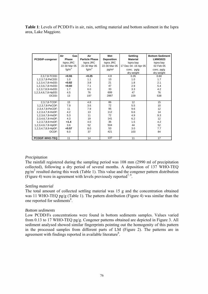
76

Table 1: Levels of PCDD/Fs in air, rain, settling material and bottom sediment in the Ispra area, Lake Maggiore.

PCDD/F-congenerAir Gas

PhaseAir

Particle PhaseWet

DepositionSettling Material

Bottom Sediment LMMS023

Ispra JRC Ispra JRC Ispra JRC Ispra bay Ispra bay22-30 Mar 05 22-30 Mar 05 22-30 Mar 05 17 Dec 04 -19 Apr 05 02 Feb 05

fg/m3 fg/m3 pg/m² conc. pg/g conc. pg/g dry weight dry weight

2,3,7,8-TCDD: <0.55 <0.25 4.8 0.35 0.601,2,3,7,8-PeCDD: 1.0 1.1 13 1.0 1.71,2,3,4,7,8-HxDD: <0.82 3.8 21 1.8 2.11,2,3,6,7,8-HxDD: <0.60 7.1 47 2.9 5.41,2,3,7,8,9-HxDD: 1.7 6.0 33 3.3 4.2

1,2,3,4,6,7,8-HpDD: 4.5 76 699 47 76OCDD: 13 197 2887 229 538

2,3,7,8-TCDF: 15 4.8 86 12 151,2,3,7,8-PeCDF: 7.9 3.6 72 5.5 102,3,4,7,8-PeCDF: 11 7.9 95 9.6 121,2,3,4,7,8-HxDF: 4.2 13 112 6.6 141,2,3,6,7,8-HxDF: 5.3 11 72 4.9 9.32,3,4,6,7,8-HxDF: 4.3 19 141 6.2 121,2,3,7,8,9-HxDF: <1.4 4.0 36 1.5 4.2

1,2,3,4,6,7,8-HpDF: 3.6 52 504 44 521,2,3,4,7,8,9-HpDF: <0.57 8.0 53 3.0 7.7

OCDF: 6.0 37 421 103 84

PCDD/F-WHO-TEQ 11 14 137 11 17 Precipitation The rainfall registered during the sampling period was 108 mm (2990 ml of precipitation collected), following a dry period of several months. A deposition of 137 WHO-TEQ pg/m2 resulted during this week (Table 1). This value and the congener pattern distribution (Figure 4) were in agreement with levels previously reported7, 9. Settling material The total amount of collected settling material was 15 g and the concentration obtained was 11 WHO-TEQ pg/g (Table 1). The pattern distribution (Figure 4) was similar than the one reported for sediments8. Bottom sediments Low PCDD/Fs concentrations were found in bottom sediments samples. Values varied from 0.13 to 17 WHO-TEQ pg/g. Congener patterns obtained are depicted in Figure 3. All sediment analysed showed similar fingerprints pointing out the homogenity of this pattern in the processed samples from different parts of LM (Figure 2). The patterns are in agreement with findings reported in available literature8.

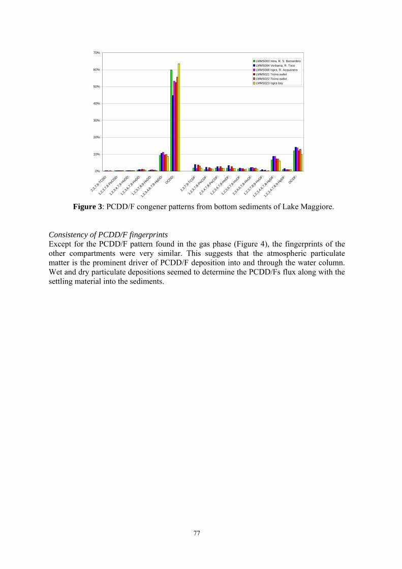
77

0%

10%

20%

30%

40%

50%

60%

70%

2,3,7,

8-TCDD:

1,2,3,

7,8-P

eCDD:

1,2,3,

4,7,8-

HxDD:

1,2,3,

6,7,8-

HxDD:

1,2,3,

7,8,9-

HxDD:

1,2,3,

4,6,7,

8-HpD

D:

OCDD:

2,3,7,

8-TCDF:

1,2,3,

7,8-P

eCDF:

2,3,4,

7,8-P

eCDF:

1,2,3,

4,7,8-

HxDF:

1,2,3,

6,7,8-

HxDF:

2,3,4,

6,7,8-

HxDF:

1,2,3,

7,8,9-

HxDF:

1,2,3,

4,6,7,

8-HpD

F:

1,2,3,

4,7,8,

9-HpD

F:

OCDF:

LMMS003 Intra, R. S. BernardinoLMMS004 Verbania, R. ToceLMMS008 Ispra, R. AcquaneraLMMS021 Ticino outletLMMS022 Ticino outletLMMS023 Ispra bay

Figure 3: PCDD/F congener patterns from bottom sediments of Lake Maggiore.

Consistency of PCDD/F fingerprints Except for the PCDD/F pattern found in the gas phase (Figure 4), the fingerprints of the other compartments were very similar. This suggests that the atmospheric particulate matter is the prominent driver of PCDD/F deposition into and through the water column. Wet and dry particulate depositions seemed to determine the PCDD/Fs flux along with the settling material into the sediments.

78

Figure 4: PCDD/F congener patterns of the deposition chain into Lake Maggiore. The fact that the PCDD/F patterns of particulate matter and sediments in LM showed a typical atmospheric long range transport signal8, demonstrated a minor impact from local sources. PCDD/F fluxes into LM during 22-30 March 2005 at Ispra bay In order to check the hypothesis that the sedimentation of PCDD/Fs into LM is mainly driven by the atmosphere, we present a comparison of the related fluxes into and through the water column, estimated on the basis of the concentration data presented in Table 1. Dry particulate matter flux into the water column was estimated on the basis of atmospheric particulate matter concentration (TSP) in Ispra air (average of 65 µg/m3 during 22-30 March 2005)5 and the related PCDD/Fs data, assuming a deposition velocity of 0.2 cm/s10-11. Wet deposition was calculated from the amount of PCDD/Fs measured in the rain sampler. The flux of settling material (SM) and the related PCDD/F flux through the water column were estimated from the sediment trap data during that time. Finally, the flux into the bottom sediment was approximated from the grab sample representing an area of 0.015 m2 and a depth of 10 cm. Assuming a sedimentation rate at the Ispra bay ranging between 0.25 – 0.5 cm per year12-13, the sediment sample would represent a sedimentation record of 20 to 40 years. Resulting fluxes are summarized in Table 2.

2,3,7,8-TCDD:

1,2,3,7,8-PeCDD:

1,2,3,4,7,8-HxD

D:

1,2,3,6,7,8-HxD

D:

1,2,3,7,8,9-HxD

D:

1,2,3,4,6,7,8-H

pDD:

OCDD:

2,3,7,8-TCDF:

1,2,3,7,8-PeCDF:

2,3,4,7,8-PeCDF:

1,2,3,4,7,8-HxD

F:

1,2,3,6,7,8-HxD

F:

2,3,4,6,7,8-HxD

F:

1,2,3,7,8,9-HxD

F:

1,2,3,4,6,7,8-H

pDF:

1,2,3,4,7,8,9-H

pDF:

OCDF:

Particle Phase

Precipitation

Settling material

Bottom sediment

Gas phase

79

Table 2: Estimate of weekly fluxes into Lake Maggiore.

Type of flux Particle deposition Wet deposition Settling material Bottom

sediment 22-30 Mar 05 22-30 Mar 05 17 Dec 04-19 Apr 05 2 Feb 05

TSP/SM/Sediment 77 mg/m2 n.d. 4.5 g/m2 7.5-15 g/m2

PCDD/Fs (WHO-TEQ) 17 pg/m2 136 pg/m2 50 pg/m2 125-250pg/m2

The PCDD/F data for dry particulate fluxes and wet deposition into LM match fairly well the PCDD/F flux of settling material taking into account, that we are comparing the weekly averages of atmospheric deposition fluxes of the last week of March 2005 with a settling material flux measured between December 04 and April 05. The flux estimate into the bottom sediment of Ispra bay is higher compared to the flux of settling material. This may be explained by the fact that the bottom sediment sample represents the whole annual cycle of sedimentation, including the atmospheric inputs during the rainy winter season, where PCDD/F and particulate matter concentrations and the related fluxes are higher than during the period in March 2005 where the data on ambient air and settling material were acquired. Despite the preliminary character of the data presented, the PCDD/Fs fingerprints and the related flux estimates suggested a prominent role of atmospheric deposition in the accumulation of PCDD/Fs in LM sediments. Acknowledgements We thank Wolfgang Mehl and Friedrich Lagler for the help with the recovery of the sediment trap.

References 1. Safe S. (1991) Environ. Carcinog. Ecotoxicol. Rev. 9: 261-302. 2. Harrad S.J. and Jones K.C. (1992) Sci. Total Environ. 126: 89-107. 3. Bruzy L.P. and Hites, R.A (1996). Environ. Sci. Technol. 30: 1797-1804. 4. U.S. EPA (1994) Health Assessment Document for 2,3,7,8-Tetrachloro-Dioxin (TCDD) and Related Compounds; United States Environmental Protection Agency: Washington, DC. 5. European Commission Joint Research Centre. European Monitoring and Evaluation Program (EMEP) Ispra Site (http://carbodat.ei.jrc.it/ccu/main.cfm). 6. Umlauf G., Bidoglio G., Christoph E.H., Kampheus J., Krüger F., Landmann D., Schulz AJ, Schwartz R., Severin K., Stachel B. and Stehr, D. The Situation of PCDD/Fs and Dioxin-like PCBs after the Flooding of River Elbe and Mulde in 2002, Acta Hydrochimica and Hydrobiologica, in press April 2005. 7. Lohmann R. and Jones K.C. (1998) Sci. Total Environ. 219 : 53-81. 8. Hagenmeier H., Lindig C. and She J. (1994) Chemosphere. 29: 2163-2174. 9. Guerzoni S., Rossini P., Molinaroli E., Rampazo G. and Raccanelli S. (2004) Chemosphere 54: 1309-1317. 10. Hillery B.R., Simcik M.F., Basu I., Hoff R.M., Strachan W.J.M., Burniston D., Chan C.H., Brice K.A., Sweet C.W. and Hites R.A. (1998) Sci. Total Environ. 32: 2216-2221. 11. Miller S.M., Green M.L., DePinto J.V. and Hornbuckle K.C. (2001) Sci. Total Environ. 35: 278-285. 12. Marchetto A., Guilizzoni P. and Lami A. Commissione Internazionale per la protezione delle acque italo-svizzere. Monitoraggio della presenza del DDT e di altri contaminati nell’ecosistema Lago Maggiore. Rapporto annuale Aprile 2003-Marzo 2004, 12.

http://carbodat.ei.jrc.it/ccu/main.cfm

80

13. Marchetto A., Guilizzoni P. and Lami, A. Commissione Internazionale per la protezione delle acque italo-svizzere. Monitoraggio della presenza del DDT e di altri contaminati nell’ecosistema Lago Maggiore. Rapporto annuale Aprile 2001-2002, 8.

81

INDUSTRIAL AND CONSUMER PRODUCTS IN THE GREAT LAKES: THE ROLE OF THE ATMOSPHERE

Keri C. Hornbuckle1, Aaron Peck2, Bryan Boulanger3, Carolyn Persoon1

1 Department of Civil and Environmental Engineering, University of Iowa, Iowa City, Iowa 52242, USA

2 National Institute of Standards and Technology, Hollings Marine Laboratory, 331 Fort Johnson Road, Charleston, South Carolina 29412 USA

3 U. S. Environmental Protection Agency, National Risk Management Research Laboratory, MS421, 26W Martin Luther King Drive, Cincinnati, Ohio 45268 USA

Introduction The presence of consumer, industrial, and agricultural products in natural systems is well known. Unfortunately the source of these chemicals is not often well understood. Source determination is difficult because of lack of data for an ecosystem, or inappropriate assumptions about the magnitudes and trends in current inputs. Atmospheric inputs, for example, are often ignored as major sources to surface waters and terrestrial systems. For some chemicals, the lack of field data completely prevents a correct evaluation of the importance of atmospheric pathways. For other compounds, the data is available, but the modeling effort is inconsistent or incomplete. It is therefore common that the atmospheric pathway is underestimated, especially for surface waters close to industrial areas. The presence of three organic compound groups in the Great Lakes of North America illustrates this point: polychlorinated biphenyls (PCBs); synthetic musk fragrances; and perfluorinated surfactants. Here, we compare these three compound groups using the structure of that classic environmental engineering tool, the mass balance model. PCBs are present in the environment of the Great Lakes as a result of historical use and discharge of PCBs from many different industries within the Great Lakes basin, including packing plants, paper mills, tanneries, machine shops, and foundries. These industries expanded in the Great Lakes at the same time PCB use expanded: between the 1930s and the mid 1970s. At this time, PCBs were common additives to oil and other substances to prevent breakdown and maintain viscosity (ATSDR, 2000). New use of PCB was discontinued in the mid-1970s and all production ceased by 1979. Since then, PCBs have been removed from active use although they are still found in high concentrations in waste disposal sites and in reservoirs of old stockpiles throughout the Great Lakes Basin. PCBs are a valuable comparison group for all persistent organic pollutants because we understand their environmental cycling and production history quite well. We are also well aware of their harmful impacts on humans and animals. Unfortunately, control of PCBs still suffers from lack of information about their current sources. Synthetic musk fragrances include nitroaromatics, polycyclics, and macrocyclic compounds. The most widely used fragrances are highly persistent and appear to exhibit low-level toxicity to aquatic organisms. Synthetic musks are fragrance additives used in soaps, perfumes, cosmetics, air fresheners, laundry detergents, and shampoos. These products are ubiquitous in the aquatic environment due to disposal of musk-containing products via water systems and incomplete removal by sewage treatment (Eschke, 2004; Peck and Hornbuckle, 2004). The musk fragrances with the highest volume of use are the

82

polycyclic musks, of which two compounds, AHTN (Tonalide®, 7-acetyl-1,1,3,4,4,6-hexamethyl-1,2,3,4-tetrahydronaphthalene) and HHCB (Galaxolide®, 1,3,4,6,7,8-hexahydro-4,6,6,7,8-hexamethylcyclopenta-γ-2-benzopyran), represented 95% of total polycyclic musk production in 1996 (Rimkus, 1999). AHTN and HHCB have been detected in human breast milk and adipose tissue (Rimkus and Wolf, 1996; Liebl et al., 2000; Zehringer and Herrmann, 2001), fish, mussels, shrimp, and otters (Leonards and deBoer, 2004). Perfluorinated compounds have recently been recognized as harmful environmental contaminants and some have been removed from the market or are undergoing regulatory review. These compounds are related to the production and use of many useful products including surface protectants, fabric treatments, and polytetrafluoroethylene (PTFE). Like the synthetic musk fragrances, the production and use information for this group of compounds is proprietary and essentially unavailable to the public. Two classes of perfluorinated organic compounds are of concern due to their widespread presence in human blood and natural systems (Giesy and Kannan, 2001; Hansen et al., 2002; Kannan et al., 2002a; Kannan et al., 2002b; Moody et al., 2002; Hoff et al., 2003; Olsen et al., 2003; Taniyasu et al., 2003a; Taniyasu et al., 2003b). The perfluorinated sulfonamides and their degradation products were produced by 3M Company in the United States as surface protectants for upholstery, carpets, and fabrics. The compounds were removed from the market in 2001 after their major degradation product, perfluorooctane sulfonate (PFOS) was found in human and animal blood worldwide. A second class of concern is the fluorinated telomers (Stock et al., 2004). These linear long chain alcohols are associated with the production, use, and distribution of surface protectants used on cooking materials as well as fabrics and carpets. These compounds are produced primarily by DuPont in the United States using a process called telemerization, hence their name. The widespread commercial and industrial usage of both classes has led to the accumulation of PFOS and perfluorooctanoic acid (PFOA) in the blood and tissues of animals and humans. However, the cause of this accumulation is not well understood, because there is very little information pertaining to sources of these compounds to the environment. Results aqnd discussion We have used the mass balance approach to illustrate the relative importance of sources of persistent organic compounds to the Great Lakes. The general mass balance equation we have applied is:

( )ACkCQAH

CkQC

dtdC

V WolWoutA

olW +−⎟

⎠

⎞⎜⎝

⎛+= ∑∑

Equation (1) where Cw is the

concentration of the compound in lake water, C is the concentration of water in a tributary or other discharge with flowrate Q, kol is the overall mass transfer coefficient, CA is the average gas-phase concentration over the lake, H the Henry’s Law Constant, A is the surface area of the lake, Cw is the water concentration, and Qw is the flow of water from the lake. For the set of compounds described here, the water concentration is nearly equal to the dissolved phase concentration in the Great Lakes. This is because of the very low suspended sediment concentrations in the Great Lakes and very low concentration of high molecular weight PCBs in the Great Lakes water column. PCBs originally entered Lakes Michigan, Erie and Ontario though local discharges from contaminated tributaries, wastewater effluents, and industrial runoff (Hornbuckle et al., in

83

press). After the ban from production and later from any new uses, the direct discharge of PCBs to the Great Lakes declined. More than 20 year after the ban, a large proportion of PCBs now enter the Great Lakes from nonpoint sources. Figure 1 represents the current understanding of all sources and losses of PCBs in Lake Michigan (U.S. Environmental Protection Agency, 2005). The mass budget was constructed after a large sampling effort that included air, water, sediment, and biota sampling throughout the lake. It is now evident that the atmosphere is the largest source of PCBs to Lake Michigan, with the majority through gas exchange. Atmospheric deposition (gas, dry particle, and wet deposition) is larger than inputs from resuspension of contaminated sediments and larger than inputs from direct discharge and contaminated tributaries. The tributary load is only about 380 kg and that includes the Fox River discharge to Green Bay. A significant portion of the PCBs discharged by the Fox River are retained or volatilized from Green Bay and never reach Lake Michigan (U.S. Environmental Protection Agency, 2005). Resuspension of contaminated sediments is an important source of PCBs to the water, but still not as large as gross atmospheric deposition. Although not considered as part of the annual mass budget, a field study of resuspension after major storms concluded that annual wintertime storms contribute as much as 400 kg of PCBs per event (Hornbuckle et al., 2004). There may be more than one major event each year, but a large fraction of that mass may immediately return to the lake floor.

Figure 1. Mass budget of inputs and losses of PCBs measured or modeled in Lake Michigan. From (U.S. Environmental Protection Agency, 2005). The importance of the atmospheric pathway is easily misjudged. For example, sediment export from contaminated tributaries as a source of PCBs to Lake Michigan is often cited as a justification for dredging (Reible and Riley, 2004). However, atmospheric releases from highly contaminated tributaries and harbors may be a larger net source of PCBs to the open lake than is the corresponding direct discharge. In Milwaukee, for example, atmospheric sources contribute about 150 kg each year to the open waters of Lake Michigan. The Milwaukee River, on the other hand, contributes only about 12 kg annually (U.S. Environmental Protection Agency, 2005; Wethington and Hornbuckle, 2005).

As are PCBs, synthetic musk fragrances are ubiquitous in the environment. In fact, two of the most commonly found polycyclic musk fragrances have been reported in virtually every environmental matrix. In Lakes Michigan and Ontario, the concentrations of AHTN (Tonalide®, 7-acetyl-1,1,3,4,4,6-hexamethyl-1,2,3,4-tetrahydronaphthalene) and HHCB (Galaxolide®, 1,3,4,6,7,8-hexahydro-4,6,6,7,8-hexamethylcyclopenta-γ-2-benzopyran) exceed the concentrations of PCBs (sum of all measured congeners) in water and in air.

84

Synthetic musk fragrances are widely found in air. Air concentrations are highest in urban locations, such as Milwaukee, WI (Peck and Hornbuckle, 2004) and Cedar Rapids, IA (Peck and Hornbuckle, In review). Urban concentrations of HHCB and AHTN are on the order of 1-5 ng/m3 and background terrestrial concentrations are about an order of magnitude less. This is similar to the range of total PCBs found in the same regions. In rural air, the concentrations and frequency of detection of the synthetic musk fragrances are comparable to (and often greater than) gas-phase pesticide concentrations (Kallenborn et al., 1999). The concentrations measured at the suburban locations in Iowa City, IA and over Lakes Erie, Ontario, and Michigan were generally intermediate of those measured at the rural and urban locations.

A mass budget analysis of synthetic musk fragrances in Lake Michigan revealed that direct discharges from wastewater treatment effluents dominate sources of these compounds to Lake Michigan (Figure 2). Atmospheric inputs were negligible by comparison. On the other hand, volatilization of synthetic musk fragrances represents an important loss mechanism for the lake. Loss via volatilization to the atmosphere is of the same order of magnitude as discharge to the downstream lake (Huron) for most musks and much greater than discharge for AHMI (Phantolide® , 6-acetyl-1,1,2,3,3,5-hexamethyldihydroindene). The mass budget analysis may explain why atmospheric concentrations of synthetic musk fragrances over Lakes Michigan, Erie, and Ontario are higher than expected for a remote region. We hypothesize that that is due to volatilization of the compounds from the waters of the Great Lakes. In terrestrial regions, like rural Iowa and Norway(Kallenborn et al., 1999), fragrances are captured by surface soils and vegetation and volatilization at a much lower rate than over water.

HHCB AHTN0.000.010.020.03

MK MX ADBI AHMI ATII0.0000.0010.0020.0030.004

Atmospheric Deposition (kg/day)

HHCB AHTN01234

MK MX ADBI AHMI ATII0.00.20.40.60.8

WWTP Discharge (kg/day)

HHCB AHTN0.0

0.5

1.0

Outflow (kg/day)

HHCB AHTN0.0

0.2

0.4

0.6

MK MX ADBI AHMI ATII01234

Volatilization (kg/day)

MK MX ADBI AHMI ATII0.00

0.04

0.08

0.12

0.00001 0.00006

Figure 2. Mass budget of inputs and losses of seven synthetic musk fragrances measured or modeled in Lake Michigan. From (Peck and Hornbuckle, 2004). Perfluorinated compounds have been found in most environmental matrices in which they have been tested. Concentrations of the end products, PFOS and PFOA, exceed concentrations of PCBs and synthetic fragrances in some matrices. For example, in Lakes Erie and Ontario the concentrations of PFOS and PFOA ranged from 21 to 70 ng/L and 27 to 50 ng/L, respectively. This is about two orders of magnitude higher than total PCBs (0.1 to 0.5 ng/L in open waters of the Great Lakes) and about ten times higher than the

85

fragrances HHCB and AHTN. The source of the compounds was examined by through a series of field sampling expeditions in the Great Lakes and subsequent modeling of potential sources(Boulanger et al., 2005a). Wastewater effluents appear to the major source of perfluorinated compounds currently entering the Great Lakes. For Lake Ontario, discharge from Lake Erie is a second major source of the compounds. Deposition fluxes from gas exchange or dry particles were measurable above analytical detection limits but were negligible compared to wastewater and upstream discharge. Volatilization is also a negligible loss mechanism relative to downstream export to the St. Lawrence River. Another input mechanism, deposition in rain, was not evaluated in our study, but has a potential to be an important source, especially near production facilities that use PFOA. The source of perflorinated compounds to the wastewater is not clear, especially for PFOS. PFOS was not a reported component of the 3M product but considered a degradation or metabolic byproduct of its parent monomer, N-EtFOSE (N-ethyl perfluorooctane sulfonamidoethanol). We hypothesized that PFOS is present in wastewater due to decay of N-EtFOSE. Through a series of microcosm studies using local wastewater mixed liquor, we found that while N-EtFOSE does decay in wastewater, it does not produce PFOS at a rate that could explain the presence of PFOS in wastewater (Boulanger et al., 2005b) . Our second hypothesis was that PFOS and other compounds measured in Great Lakes water originated from consumer products directly, particularly the 3M product that was removed from the market in 2000: Scotchgard. Analysis of an archived can of Scotchgard indicated the presence of PFOS, PFOA and all the remaining compounds in our analytical method. We concluded that the presence of PFOS in the Great Lakes can at least partly be explained by the use and subsequent disposal of the consumer product.

Figure 3. Mass budget of inputs and losses of eight perfluorinated surfactants measured or modeled in Lake Ontario. From (Boulanger et al., 2005a).

86

References ATSDR (2000). Toxicological profile for polychlorinated biphenyls (PCBs), U.S. Department of

Health and Human Services, Agency for Toxic Substances and Disease Registry, Atlanta GA. 948 pp.

Boulanger, B, Peck, AM, Schnoor, JL and Hornbuckle, KC (2005a). Mass budget of perfluorooctane surfactant in Lake Ontario. Environmental Science & Technology 39 (1): 74-79.

Boulanger, B, Vargo, JD, Schnoor, JL and Hornbuckle, KC (2005b). Evaluation of perfluorooctane surfactants in a wastewater treatment system and in a commercial surface protection product. Environmental Science & Technology 39 (15): 5524-5530.

Eschke, H-D (2004). Synthetic musks in different water matrices. In Synthetic Musk Fragrances in the Environment, G. G. Rimkus, Ed. New York, Springer-Verlag, pp 17-28.

Giesy, JP and Kannan, K (2001). Global Distribution of Perfluorooctane Sulfonate in Wildlife. Environmental Science & Technology 35 (7): 1339-1342.

Hansen, KJ, Johnson, HO, Eldridge, JS, Butenhoff, JL and Dick, LA (2002). Quantitative Characterization of Trace Levels of PFOS and PFOA in the Tennessee River. Environmental Science & Technology 36 (8): 1681-1685.

Hoff, PT, Van de Vijver, K, Van Dongen, W, Esmans, EL, Blust, R and De Coen, WM (2003). Perfluorooctane Sulfonic Acid in Bib (Trisopterus luscus) and Plaice (Pleuronectes platessa) from the Western Scheldt and the Belgian North Sea: Distribution and Biochemical Effects. Environmental Toxicology and Chemistry 22 (3): 608-614.

Hornbuckle, KC, Carlson, DL, Swackhamer, DL, Baker, JE and Eisenreich, SJ (in press). PCBs in the Great Lakes. In Persistent Organic Pollutants in the Great Lakes, R. A. Hites, Ed. Heidelberg, Springer-Verlag, pp.

Hornbuckle, KC, Smith, GL, Miller, SM, Eadie, BJ and Lansing, MB (2004). Magnitude and origin of polychlorinated biphenyl (PCB) and dichlorodiphenyltrichloroethane (DDT) compounds resuspended in southern Lake Michigan. J. Geophysical Res.-Oceans 109: Art. No. C05017 MAY 18.

Kallenborn, R, Gatermann, R, Planting, S, Rimkus, GG, Lund, M, Schlabach, M and Burkow, IC (1999). Gas chromatographic determination of synthetic musk compounds in Norwegian air samples. Journal of Chromatography A 846 (1-2): 295-306.

Kannan, K, Choi, JW, Iseki, N, Senthilkumar, K, Kim, DH, Masunaga, S and Giesy, JP (2002a). Concentrations of Perfluorinated Acids in Livers of Birds from Japan and Korea. Chemosphere 49 (3): 225-231.

Kannan, K, Corsolini, S, Falandysz, J, Oehme, G, Focardi, S and Giesy, JP (2002b). Perfluorooctanesulfonate and Related Fluorinated Hydrocarbons in Marine Mammals, Fishes, and Birds from Coasts of the Baltic and the Mediterranean Seas. Environmental Science & Technology 36 (15): 3210-3216.

Leonards, PEG and deBoer, J (2004). Synthetic musks in fish and other aquatic organisms. In Synthetic Musk Fragrances in the Environment, G. G. Rimkus, Ed. New York, Springer-Verlag, pp 49-84.

Liebl, B, Mayer, R, Ommer, S, Sonnichsen, C and Koletzko, B (2000). Transition of nitro musks and polycyclic musks into human milk. Short and Long Term Effects of Breast Feeding on Child Health 478: 289-305.

Moody, CA, Martin, JW, Kwan, WC, Muir, DCG and Mabury, SA (2002). Monitoring Perfluorinated Surfactants in Biota and Surface Water Samples Following an Accidental Release of Fire-Fighting Foam into Etobicoke Creek. Environmental Science & Technology 36 (4): 545-551.

Olsen, GW, Hansen, KJ, Stevenson, LA, Burris, JM and Mandel, JH (2003). Human Donor Liver and Serum Concentrations of Perfluorooctanesulfonate and Other Perfluorochemicals. Environmental Science & Technology 37 (5): 888-891.

Peck, AM and Hornbuckle, KC (2004). Synthetic musk fragrances in Lake Michigan. Environmental Science & Technology 38 (2): 367-372.

87

Peck, AM and Hornbuckle, KC (In review). Synthetic Musk Fragrances in Urban and Rural Air of North America.

Reible, DD and Riley, K (2004). TOSC Review of Indiana Harbor and Canal Dredging and Disposal Alternatives Analysis. Conducted at the request of the Grand Calumet Task Force and Citizens for a Clean Environment, Technical Outreach Services for Communities (TOSC) Program, Michigan State University, East Lansing, MI. 23 pp.

Rimkus, GG (1999). Polycyclic musk fragrances in the aquatic environment. Toxicology Letters 111 (1-2): 37-56.

Rimkus, GG and Wolf, M (1996). Polycyclic musk fragrances in human adipose tissue and human milk. Chemosphere 33 (10): 2033-43.

Stock, NL, Lau, FK, Ellis, DA, Martin, JW, Muir, DCG and Mabury, SA (2004). Perfluorinated Telomer Alcohols and Sulfonamides in the North American Troposphere. Environmental Science & Technology 38 (4): 991-996.

Taniyasu, S, Kannan, K, Horii, Y, Hanari, N and Yamashita, N (2003a). A Survey of Perfluorooctane Sulfonate and Related Compounds in Water, Fish, Birds, and Humans from Japan. Environmental Science & Technology 37 (12): 2634-2639.

Taniyasu, S, Kannan, K, Horii, Y, Hanari, N and Yamashita, N (2003b). A survey of perfluorooctane sulfonate and related perfluorinated organic compounds in water, fish, birds, and humans from Japan. Environmental Science & Technology 37 (12): 2634-2639.

U.S. Environmental Protection Agency (2005). Lake Michigan Mass Balance Study Loadings Report. pp.

Wethington, DM and Hornbuckle, KC (2005). Milwaukee, WI, as a source of atmospheric PCBs to Lake Michigan. Environmental Science & Technology 39 (1): 57-63.

Zehringer, M and Herrmann, A (2001). Analysis of polychlorinated biphenyls, pyrethroid insecticides and fragrances in human milk using a laminar cup liner in the GC injector. European Food Research and Technology 212 (2): 247-251.

88

PERSISTENT ORGANOHALOGENS AND CURRENT USE PESTICIDES IN REMOTE LAKE WATERS, SEDIMENTS AND ICECAPS

D.C.G. Muir1, C. A. Teixeira1, M. Alaee1, and M. Hermanson2

1National Water Research Institute, Environment Canada, Burlington, ON, Canada

2Department of Chemistry, University of Pennsylvania, Philadelphia, PA 19104, USA Introduction Recent regional and global protocols on persistent organic pollutants (POPs) have included criteria for identification of these substances such as “are prone to long-range trans-boundary atmospheric transport (LRAT) and deposition” 1 and “Monitoring data showing that long-range environmental transport of the chemical, with the potential for transfer to a receiving environment, may have occurred via air, water, or migratory species”2. Studies demonstrating LRAT and deposition for organic chemicals other than the 12 on the UNEP POPs list or the 4 additional substances/chemical groups listed by UNECE (polyaromatic hydrocarbons (PAHs), hexachlorocyclohexanes (HCH), hexabromobiphenyl, and chlordecone) are very limited. For example, routine air-monitoring in the Canadian Arctic includes essentially only the 10 UNEP POPs plus PAHs, and current use pesticides endosulfan and lindane 3. This is also the case for air measurements by the Integrated Atmospheric Deposition Network (IADN) in the Great Lakes 4. In the European Arctic the analyte list is shorter and does not include endosulfan 3. Measurements of atmospheric transport to the Antarctic are also limited to a suite of POPs 5. A recent, ongoing, global survey of air using passive air samples (GAPS) is focusing on the same suite although PBDEs will be added 6. A lot has been learned about global environmental fate, persistence and transport of semi-volatile organics from studies on PCBs, chlorobenzenes and HCH isomers, however, a much broader array of chemicals needs to be examined if we are to fully understand the fate of the semi-volatile chemicals in commerce. A recent categorization of 11,300 chemicals in commerce 7 revealed that 37% of the chemicals had predicted air-water partition coefficients (log KAW) >-5 and <-1 i.e. high LRAT potential if persistent in the atmosphere 8 and about 24% of the latter group (930 substances) had predicted atmospheric oxidation half-life of >1 day 7. Current use pesticides (CUPs) share many physical-chemical properties with organics on the various “existing chemicals” lists except that, unlike most commercial chemicals, their basic phys-chemical properties are known, as is their use area and application time. While use of a few organochlorine (OC) insecticides (lindane, endosulfan) continues, the pesticides that are currently in widest use tend to have much greater polarity and water solubility than legacy OCs and are more biodegradable. CUPs which can still possess considerable persistence, include herbicides such as the triazines (atrazine) and the acetanilides (alachlor, metolachlor), organophosphate (OP) insecticides (chlorpyrifos, diazinon, disulfoton), as well as fungicides (chlorothalonil). CUPs have generally been measured in regional programs within a few hundred kms of sources areas 9. At least 80 CUPs have been detected in precipitation and 30 in air in studies in Europe, mainly in France, Germany, the Netherlands and the UK 9. In North America, investigation of CUPs has been more limited. The IADN program has included selected herbicides such as atrazine in precipitation but not air 4. LRAT of CUPs from California’s central valley to the Sierra Nevada has been well documented 10, 11. Regional atmospheric transport of triazine and acetanilide herbicides used in corn production was also apparent from

89

measurements of these herbicides in precipitation in the US Midwest 12, in remote, non-agricultural, locations on Isle Royale in Lake Superior 13 and in northwestern Ontario14. Although precipitation, gas and particle phase measurements are needed to fully understand and quantify LRAT and deposition of CUPs and POPs, measurements of these media are not always available, particularly in remote areas. This is because samplers require reliable electrical power, protected sites away from local sources, and trained personnel. While PAS are a viable alternative for air measurements more work is needed on their performance with CUPs having high polarity; they have mainly been used with POPs 15. Organics that are carried on atmospheric particles may not be efficiently sampled passively. Other media such as lake waters, sediments and ice cores can be used as substitutes for both particle-borne and polar compounds to obtain a preliminary assessment of presence in important environmental compartments and, in some cases, good estimates of current deposition. This is the focus of this paper. Methods Lake waters: Water was collected from 39 lakes in Canada and nearby northern US States for determination of selected CUPs (Figure 1). Approximately 34 of 39 lakes had no agricultural activity within 10 km and most were 100’s of kilometers from agricultural areas. Muir et al. 16, 17 list the names, geographical coordinates and surface area of the study lakes. Samples were collected mid-summer from July 1999 to July 2003. Large volume lake water samples (19 L or 100 L) collected from the top 1 m, in duplicate, excluding surface layers, using pre-cleaned stainless steel containers (19L). The water was shipped to the laboratory (30 of 40 locations) or extracted on site (10 locations) by pumping water through XAD-2 resin columns. The columns were prepared in a clean room (positively pressured HEPA™ and carbon filtered air) using XAD-2 that had been thoroughly cleaned by Soxhlet extraction 16. Ten lakes in Ontario were studied in more detail by monthly collection of waters from epilimnion and hypolimnion from May through July 2003 17. Sediments: Sediment cores (10 cm or 6.5 cm diameter) from lakes along a south to north transect in Canada and nearby northern US States for determination of POPs and brominated diphenyl ethers 18. Cores were sliced either at 0.5 cm intervals (Arctic lakes) or 1 cm intervals (those south of 55oN)18. In the laboratory, wet sediments were centrifuged to remove excess water. Moisture content was determined on a subsample prior to centrifugation. The wet sediment was mixed with a drying agent and extracted on a accelerated solvent extractor (Dionex Instruments, Oakville ON) using dichloromethane. The extract was subsequently treated to remove sulfur and chromatographed on an activated silica column to separate PCBs from PBDEs. Sediment cores were dated using the Pb210 technique and slices dated to pre-1900 were extracted and used as blanks for PBDE analysis. Glacial ice: Samples were obtained from a 118-m ice core collected from the summit of Austfonna icecap (79.48°N, 24°E, 740 m above sea level) in Svalbard. Austfonna is the largest Eurasian polar ice cap located in arctic Norway, where pesticides were never produced and likely were never used (Figure 1) Characteristics of the core are discussed by Isaksson et al. 20. The estimated accumulation rate is ~0.5 m (H2O equivalent) yr-1 and the melt index is 40-67%, suggesting that the summer melt penetrates no more than 5 years of the near-surface snow and firn 21. Samples from the upper 40 m dating from 1943 ± 5 yrs to 1998 were used for analysis and lower depths were used as blanks; no blank corrected values appeared below 40 m depth. Ice core segments making up a sample were placed in a stainless steel can and melted to a final temperature not >5°C. CUPs were separated

90

from melted ice by pumping 200-250 mL/min through Teflon-walled extraction columns filled with XAD-2 resin as described for water22. GC-MS analysis: CUPs in lake water and glacial ice extracts were quantified by gas chromatography (GC)-low resolution mass spectrometry (electron ionization mode and negative chemical ionization mode) using an Agilent 6890 GC and 5973 mass selective detector (Agilent Technologies, Palo Alto CA). CUPs were quantified using authentic external standards. Quality assurance steps included pre-spiking with deuterated fenitrothion and atrazine to measure breakthrough, and the analysis of field blanks (XAD columns shipped to the laboratory where extractions were carried out and returned with sample columns) 16. PBDEs in sediment extracts were determined by GC-high-resolution MS in electron impact mode following the method of Luross et al. 19. Results and Discussion CUPs in lake waters: Surface waters were analysed for as many as 45 CUPs by GC-MS. These 45 were chemicals in wide use in Ontario and the Great Lakes region 23, 24. Nine CUPs were consistently detected including corn herbicides atrazine and its degradation product, DEA, metolachlor, alachlor and dacthal, the fungicide chlorothalonil, the organophosphate insecticides chlorpyrifos, disulfoton and diazinon and the OC insecticide endosulfan (Table 1, Figure 2). Agreement between duplicate samples was acceptable for all nine CUPs (<30% relative % differences). By far the most prominent pesticide was atrazine, which was present at elevated concentrations (mean 81 ng/L) in 5 lakes that receive agricultural runoff in northern New York State and southern Ontario. Atrazine and DEA were also readily detectable in remote lakes in the mid-latitudes (mean = 7.2 ng/L) and in some sub-Arctic and Arctic lakes (7 of 15) but at levels approaching detection limits (Table 1, Figure 2). The prominence of atrazine in remote mid-latitude lakes reflects its continued widespread annual use in corn production 23, 24. Table 1. Mean and range of concentrations and frequency (Fr) of detection of current use pesticides in lake surface waters (ng/L). Lakes are categorized as having agricultural inputs or remote lakes in mid-latitudes, sub-Arctic and Arctic locations. CUP Agricultural inputs Remote lakes 40-50 oN Remote lakes 50-60 oN Arctic lakes >70 oN N 5 20 8 7 Mean min max Fr Mean min max Fr Mean min max Fr Mean min max Fr Desethyl-atrazine 24.9 6.87 56.6 5 2.56 0.07 6.55 20 0.48 <0.01 1.56 4 0.07 <0.01 0.49 1 Atrazine 56.1 1.32 128 5 4.65 0.16 20.1 20 0.59 <0.01 2.68 3 0.08 <0.01 0.45 2 Total Atraz 81.0 13.9 184 5 7.21 0.23 26.7 20 1.07 <0.01 4.21 5 0.18 <0.01 0.61 2 Alachlor 0.69 <0.01 1.48 3 0.62 <0.01 4.25 13 0.17 <0.01 0.53 3 0.01 <0.01 0.06 2 Chlorpyrifos 0.41 0.05 1.03 5 0.50 <0.01 2.87 14 <0.01 <0.01 <0.01 0 0.23 <0.01 1.60 2 Chlorthalonil 0.20 <0.01 0.58 4 0.34 <0.01 5.35 12 0.10 <0.01 0.77 1 0.41 <0.01 2.80 4 Dacthal 0.15 0.05 0.27 5 0.08 0.02 0.26 20 0.05 0.03 0.11 8 0.03 0.01 0.07 7 Diazinon 1.23 <0.01 2.83 4 2.06 <0.01 9.70 17 2.77 <0.01 5.24 6 0.63 <0.01 1.96 3 Disulfoton 0.37 <0.01 1.15 3 0.70 <0.01 4.95 16 1.20 <0.01 3.00 5 0.03 <0.01 0.10 2 α-endosulfan 0.09 0.05 0.13 2 0.05 0.00 0.13 10 - - - 0.001 0.001 0.001 1 Endosulfan-SO4 0.06 0.06 0.07 2 0.13 0.04 0.22 8 - - - <0.001 <0.01 <0.01 0 Metolachlor 9.57 4.34 22.5 5 1.10 0.15 4.47 20 0.62 <0.01 1.36 7 0.42 <0.01 1.13 5 Pendimethalin 0.52 <0.01 1.42 2 0.09 <0.01 0.56 9 <0.01 <0.01 <0.01 0 1.07 <0.01 7.51 1

The acetanilide herbicides, metolachlor and alachlor were also prominent in the lakes receiving agricultural runoff and in mid-latitude remote lakes (Table 1, Figure 2). Metolachlor was also detectable in 12 of 15 sub-Arctic and Arctic lakes. Metolachlor

91

continues to be used in large quantities in the US mid-west and in southern Ontario, while alachlor is used solely in the US. The OP insecticides chlorpyrifos, diazinon and disulfoton were detected in lakes receiving agricultural inputs as well as in remote lakes. Concentrations ranged widely and, unlike the herbicides, there was no distinct difference between lakes receiving agricultural inputs and other mid-latitude lakes. Also prominent in a few lakes was the fungicide chlorothalonil, which is widely used in the Great Lakes region as a fungicide. It was present at sub ng/L concentrations in Ontario lakes, however, its highest concentration (2.8 ng/L) was in a meltwater pond on Ward Hunt Island in the Canadian high arctic. Dacthal, a minor use herbicide used on specialty vegetable crops 23, 24 was detectable in all 39 lakes at sub ng/L concentrations. Endosulfan was determined in only 13 lakes (by use of GC-NIMS) and was detected in all samples. Endosulfan sulfate was also present at similar and sometimes higher concentrations than α−endosulfan, while β−endosulfan was generally not detectable. Sediment cores: Decabromodiphenyl ether (BDE 209) was detectable in recent sediments from all lakes investigated in Ontario and Québec and in northern New York State, but was near or at detection limits in cores collected north of 55oN (Table 2). BDE 209 was detected only in recent slices of all cores including Lake Ontario which, unlike the other lakes, likely receives direct

Table 2. Sediment core locations, sedimentation rates and concentrations of BDE209

Lake Location Collection Date

Latitude Longitude Average Sedimentation g m-2 yr-1

ΣPCB (pg/g dw)

BDE 209 (pg/g dw)

AX-AJ Nunavut (Arctic) 1998 80°00'N 87°00'W 110 4,400 75 Romulus Nunavut (Arctic) 2000 79°54'N 85°06'W 780 3,500 <100 Char Nunavut (Arctic) 1997 74°40'N 94°50'W 100 2,400 42 B2-1 Northern Québec 2000 57o45'N 76o10'W 150 1,700 <100 Dasserat Western Québec 2000 48°16'N 79°26'W 120 6,100 561 Opeongo Eastern Ontario 1998 45°22'N 78°22'W 120 9,800 8180 Connery Pond Upper NY State 2001 44º20’N 73º45’W 150 3,500 1147 Lake Ontario Ontario/NY State 1998 43o26’N 79o24’W 500 250,000 112,000

inputs of BDE 209 from municipal waste treatment effluents and other urban sources. Both Lake Opeongo and Connery Pond are situated in State parks and would likely have received BDE 209 inputs only from atmospheric deposition although inputs from use of boats and other equipment on the lake cannot be ruled out. The three high Arctic lakes had much lower fluxes of BDE 209 consistent with their remote locations. Romulus Lake had a very high sedimentation rate compared to the other Arctic lakes (Table 2) which may explain the non-detectable levels of PBDEs in this core. Unlike BDE 209, PCBs did not show as distinct a decline with latitude, reflecting their transport mainly in the gas phase while BDE 209 is likely to be on particles 15. CUPs in the Austfonna ice-core: Historical concentration profiles of 37 compounds were investigated in the ice core samples from Austfonna. Nine compounds were analyzed but not detected, including the DDT group, endrin, endosulfan-sulfate, chlorthalonil, pirimphos methyl, and oxons of chlorpyrifos and diazinon. Twenty compounds were observed in discontinuous

92

layers and include eight OCs (aldrin, α-endosulfan, β-endosulfan, endrin aldehyde, heptachlor, heptachlor epoxide, α-HCH, γ-HCH), seven OPs (dacthal, dimethoate, disulfoton, ethion, fonofos, guthion, and imidan), four herbicides and degradation products (alachlor, desethylatrazine, hexazinone and pendimethalin), and a fungicide (flutriafol). Eight compounds with continuous profiles in the core were OPs chlorpyrifos, terbufos, diazinon, methyl parathion, and fenitrothion, OC inisecticides methoxychlor and dieldrin, and metolachlor (Figure 3). Conclusions Our findings of CUPs and BDE 209 in regions far from their use are confirmed by several other studies of remote lakes in North America and Greenland and of Russian icecaps 13, 25,

26. Siskiwit Lake, an isolated lake on Isle Royale in Lake Superior had average annual atrazine concentrations ranging from 11-16 ng/L in surface water sampled in 1991-1993 13 similar to our remote, mid-latitude lakes in Ontario. A previous study of CUPs in snow from Russian icecaps found higher OCs and similar concentrations of several OP insecticides and acetanilide herbicides 26. The fact that OP insecticides were found in water of remote lakes and glacial ice suggests that a much wider range of chemicals can be transported to remote regions than predicted based on atmospheric reaction rates. Periods of low OH radical concentrations and limited precipitation could allow otherwise reactive chemicals to be transported long distances 16. Low temperatures may preserve them particularly in icecaps and cold, oligotrophic lakes. Similarly transport during dry periods may explain the presence of BDE 209, which is associated with air-borne particles and possibly protected from photolysis or reactions with OH radical. References 1. UNECE, 1998. Convention on Long-range Transboundary Air Pollution, Aarhus Protocol on

Persistent Organic Pollutants (POPs) United Nations Economic Commission for Europe: Geneva, Switzerland. 49.

2. UNEP, 2001. Final Act of the Conference of Plenipotentiaries on The Stockholm Convention On Persistent Organic Pollutants. United Nations Environment Program: Geneva, Switzerland. 44.

3. de Wit, C.A., A.T. Fisk, K.E. Hobbs, D.C.G. Muir, G.W. Gabrielsen, R. Kallenborn, M.M. Krahn, R.J. Norstrom, and J.U. Skaare, 2004. AMAP Assessment 2002: Persistent Organic Pollutants in the Arctic. . Arctic Monitoring and Assessment Programme (AMAP): Oslo. 310 pp.

4. Integrated Atmospheric Deposition Network, 2004. Background document. in http://www.msc-smc.ec.gc.ca/iadn/overview/background_e.html, Environment Canada, Meteorological Service of Canada: Toronto, ON.

5. Dickhut, R., A. Cincinelli, M. Cochran, and H.W. Ducklow, 2005. Atmospheric Concentrations and Air-Water Flux of Organochlorine Pesticides along the Western Antarctic Peninsula. Environ. Sci. Technol. 39: 465-470.

6. Gallardo, K.P., T. Harner, F. Wania, D.C.G. Muir, L.A. Barrie, and K.C. Jones, 2005. Global Atmospheric Passive Sampling (GAPS) Study. Organohalogen Cmpds.

7. Environment Canada, 2005. Categorization and Screening of the Domestic Substances List. Path forward towards ecological prioritization of substances for assessment. Ottawa, ON. 18.

8. Fenner, K., M. Scheringer, M. MacLeod, M. Matthies, T. McKone, M. Stroebe, A. Beyer, M. Bonnell, A.C. Le Gall, J. Klasmeier, D. Mackay, D. van de Meent, D. Pennington, B. Scharenberg, N. Suzuki, and F. Wania, 2005. Comparing Estimates of Persistence and Long-Range Transport Potential among Multimedia Models Environ. Sci. Technol. 39: 1932-1942.

93

9. van Dijk, H.F.G. and R. Guicherit, 1999. Atmospheric Dispersion of Current-Use Pesticides: A Review of the Evidence from Monitoring Studies Water Air Soil Poll. 115: 21-70

10. Zabik, J.M. and J.N. Seiber, 1993. Atmospheric transport of organophosphate pesticides from California's Central Valley to the Sierra Nevada mountains. J. Environ. Qual. 22: 80-90.

11. McConnell, L.L., J.S. LeNoir, S. Datta, and J.N. Seiber, 1998. Wet deposition of current-use pesticides in the Sierra Nevada mountain range, California, USA. Environ. Toxicol. Chem. 17: 1908-1916.

12. Goolsby, D.A., E.M. Thurman, M.L. Pomes, M.T. Meyer, and W.A. Battaglin, 1997. Herbicides and their metabolites in rainfall: Origin, transport, and deposition patterns across the midwestern and northeastern United States, 1990-1991. Environ. Sci. Technol. 31: 1325-1333.

13. Thurman, E.M. and A.E. Cromwell, 2000. Atmospheric transport, deposition and fate of triazine herbicides and their metabolites in pristine areas at Isle Royale National Park. Environ. Sci. Technol. 34: 3079-3085.

14. Rawn, D.F., T.H.J. Halldorson, and D.C.G. Muir, 1998. Atmospheric Transport and Deposition, an Additional Input Pathway for Atrazine to Surface Waters in Triazine Herbicides: Risk Assessment, ACS Books: Washington, DC. 158-176.

15. Wania, F. and C.B. Dugani, 2003. Assessing the long-range transport potential of polybrominated diphenyl ethers: A comparison of four multimedia models. Environmental Toxicology and Chemistry. 22: 1252-1261.

16. Muir, D.C.G., C. Teixeira, and F. Wania, 2004. Empirical and modeling evidence of regional atmospheric transport of current-use pesticides. Environ. Toxicol. Chem. 23: 2421-2432.

17. Muir, D., C. Teixeira, X. Wang, and C.H. Chan, Spatial/Temporal trends of current use pesticides in surface waters and precipitation in Ontario. 2004, National Water Research Institute: Burlington, ON. p. 9.

18. Muir, D. , M. Douglas, R. Pienitz, W. Vincent, F. Wania. 2002. Sources, Long Range Transport and Impacts of New and Old POPs Inferred from Date lake Sediment Cores and Lake waters. TSRI Project #206 Final Report, Health Canada, Ottawa. 56pp.

19. Luross, J.M., M. Alaee, D.B. Sergeant, C.M. Cannon, D.M. Whittle, K.R. Solomon, and D.C.G. Muir, 2002. Spatial distribution of polybrominated diphenyl ethers and polybrominated biphenyls in lake trout from the Laurentian Great Lakes. Chemosphere. 46: 665-672.

20. Isaksson, E., M.H. Hermanson, S. Hicks, M. Igarashi, K. Kamiyama, J. Moore, H. Motoyama, D.C.G. Muir, V. Pohjola, R. Vaikmäe, R.S.W. van de Wal, and O. Watanabe, 2003. Ice cores from Svalbard - useful archives of past climate and pollution history. Phys. Chem. Earth. 28: 1217-1228.

21. Tarussov, A., 1995. The Arctic from Svalbard to Severnaya Zemlya: climatic reconstructions from ice cores. in Climate Since A. D. 1500, R.S. Bradley and P.D. Jones, Editors, Routledge: London, UK. 505-516.

22. Hermanson, M.H., E. Isaksson, C. Teixeira, D.C.G. Muir, K. Compher, Y.-F. Li, M. Igarashi, and K. Kamiyama, 2005. Current-use and legacy pesticide history in the Austfonna Ice Cap, Svalbard, Norway. Environ. Sci. Technol. In press.

23. McGee, B., H. Berges, and K. Callow, 2004. Survey of Pesticide Use in Ontario, 2003, Guelph, ON: Ontario Ministry of Agriculture and Food. 22.

24. NCFAP, 2001. National pesticide use database. http://www.ncfap.org/ database/summary/default.asp.: Washington, DC.

25. Malmquist, C., R. Bindler, I. Marrenberg, B. Van Bavel, E. Karlsson, N.J. Anderson, and M. Tysklind, 2003. Time trends of selected persistent organic pollutants in lake sediments from Greenland. Environ. Sci. Technol. 37: 4319-4324.

26. Boyd-Boland, A.A., S. Magdic, and J.B. Pawliszyn, 1996. Simultaneous determination of 60 pesticides in water using solid-phase microextraction and gas chromatography-mass spectrometry. Analyst. 121: 929-938.

http://www.ncfap.org/

94

Lake water - remote

0 1000 km

Lake water - agricultural area Sediment cores

70oN 80oN

60oN

50oN

40oN

USA

USA

Greenland Svalbard

Austfonna 80oN

70oN

Alaska

Yukon

Northwest Territories

Nunavut

Glacial Ice core

Canada

0 500 kmNorway

40 50 60 70 800.01

0.1

1

10

100 desethylatrazine atrazine

40 50 60 70 800.01

0.1

1

10 disulfoton

40 50 60 70 800.01

0.1

1

10 diazinon

40 50 60 70 80

0.01

0.1

1dacthal

40 50 60 70 800.01

0.1

1

10chlorpyrifos

40 50 60 70 800.001

0.01

0.1

1a-endosulfan

Latitude

Con

cent

ratio

n (n

g/L)

Figure 1. Location of lake waters and the glacial ice core that were analysed for current use pesticides and the sediment cores that were analysed for PCBs and PBDEs Figure 2. Concentrations versus latitude for six CUPs in lake surface waters. Non-detects were assigned a value of 0.01 ng/L except for α-endosulfan (MDL = 5 x 10-4 ng/L) and dacthal (MDL = 5 x 10-3 ng/L)

95

Figure 3. Concentration trends of five OP insecticides, two OC insecticides and the herbicide metolachlor in an ice-core from the Austfonna ice cap (Svalbard)

0

10

20

30

Chlorpyrifos

Dep

th, m

0

10

20

30

Terbufos

0

10

20

30

Diazinon

0

Concentration, ng/L

Fenitrothion

0 5 10 15 20 25 30 35

10

20

30

40

Methoxychlor- 1992

- 1998

- 1986- 1979- 1972- 1964- 1957

- 1992

- 1998

- 1986

- 1979- 1972- 1964- 1957

- 1992

- 1998

- 1986- 1979- 1972- 1964- 1957- 1953

- 1953

- 1953

Dieldrin

Methyl Parathion- 1992- 1986- 1979- 1972- 1964- 1957

0 4 102 86

- 1953

- 1998

Metolachlor

96

THE ROLE OF HIGH MOUNTAINS IN THE GLOBAL TRANSPORT OF

PERSISTENT ORGANIC POLLUTANTS

Marco Vighi, Antonio Finizio, Sara Villa

Department of Environmental Sciences, University of Milano Bicocca, Piazza della Scienza 1, 21126 Milano, Italy

Introduction Due to their properties, POPs are ubiquitous and have been detected even in remote regions far from emission sites, since the late sixties1, 2. The major transport compartment for POPs is the atmosphere3, 4 and transport patterns have been described as a function of physical-chemical properties and partition mechanisms5, 6. The migration of POPs to the poles was recognised in the 1980s as the consequence of evaporation, especially in hot climates, and deposition in cold environments7. The role of Polar Regions as “cold condensers” for Persistent Organic Pollutants (POPs) has been extensively studied during the past decades. High mountains can also be considered as “remote cold areas”, free from direct contamination, but relatively close to emission areas. The role of mountains as cold condensers was first hypothesized in the early 1990s 8 but there is still a significant gap in our knowledge on the transport, deposition and behaviour of POPs in the high mountain environment9. The few data available from the Canadian Rocky Mountains show that, with increasing altitude, organochlorine pesticides in snow can increase by factors of 10 to 10010. A number of studies in European upland regions have measured concentrations of these chemicals in snow, upland lakes and glacier ice11-13. The potential of POPs to reach relatively high concentrations in mountain environments, as well as their biomagnification potential, raise the possibility of detrimental effects to upland ecosystems. Higher trophic levels in mountains may be at risk from neurobehavioral, and immuno-deficient effects due to exposure to these contaminants. Furthermore, glaciers may contribute significantly to POPs contamination of sub-alpine aquatic environments14, but the effects are largely unknown. Moreover, glacier contribution could be increased by ice-melting due to global warming15. In this frame, a SETAC Workshop on “The Role of High Mountains in the Global Transport of Persistent Organic Pollutants” was held in Milano 1-3 July 2004. The Workshop was organised into four sessions, broadly covering the following areas:

1) The role of high mountain areas as cold condensers for POPs 2) The dynamics and distribution of persistent organic pollutants in snow and ice 3) Understanding and modelling local and global transport patterns of POPs by

studying high mountains 4) The risk to mountain ecosystems through exposure to POPs.

Some of the major conclusions and outcomes of the workshop will be presented below. The role of high mountains as cold condensers for POPs

The potential of high-altitude ecosystems as “cold-traps” for POPs, as well as for current used pesticides (CUPs) is documented by research projects developed in many mountain areas of the world, such as Canadian and US Rocky Mountains, Himalaya, Alps, Andes9,

13, 16, 17.

97

However, the effectiveness of mountains as cold condenser is depending on various factors:

1. Local meteorological factors, such as precipitation rate and type (rain, snow), wind direction, humidity, temperature etc.

2. Orographic structure. More specifically, the role of spatial gradients has been underlined as a key factor for understanding the behaviour of chemicals in high mountains. More studies are needed to specify the role of altitude at the different latitudes

3. Proximity to potential sources/ densely populated areas 4. Geological and vegetational formations (e.g., altitude, surface type, vegetation

association).

Today, more information on atmospheric transport and fate of POPs in Polar Regions is available compared with high-alpine environments. Although certain similarities between polar and high-altitude environments exist, the scientific knowledge derived from polar research should not be automatically translated to high-mountainous regions without additional experimental research. In general, the substantial lack of data on “cold trapping properties”, deposition patterns and environmental distribution of POPs in tropical high-mountainous regions is stated. Thus, research priorities should be given to studies in tropical high mountainous regions.

In contrast to latitudinal atmospheric long-range transport, the altitudinal transport into high mountains can take place over relative short distances from potential sources into the pristine alpine environments. Thus, relatively “short living” compounds, not suitable for latitudinal long-range transport, may be found in high altitude environments. This was confirmed by first findings of current used pesticides (CUPs) in the US mountains9. Also atmospheric particle-mediated transport of chemicals (such as that of PAHs) is possible and meaningful in the mountains, while it is generally considered not relevant on a latitudinal gradient. Therefore, for the monitoring of POPs in alpine environments, new priority criteria for the selection of target analytes must be selected, including also chemicals with lower half-lives than conventional POPs.

The dynamics and distribution of persistent organic pollutants in snow and ice

In recent years, there has been a significant development in our understanding of air-snow partitioning, including the role of crystal morphology (specific surface area), and the partition coefficient between the snow crystal interface and air (Kia)18. From preliminary studies, we know that snow pack and ice are heterogeneous media, and considerable exchange of POPs takes place between snow and air during snow pack maturation and firnification. Photolytic transformation in snow can dramatically affect chemical composition of pollutants19. Vertical distributions of contaminants in snow pack reflect variations in deposition, and are significantly modified by post-depositional processes20. In spite of these advances, considerable gaps exist in our understanding the fate of POPs in snow. For example, the role of wind-pumping on air-surface exchange has not yet been studied, though models suggest that it affects the snow-air exchange. There was some debate over which partitioning descriptor (Kia, Henry’s Law, vapour pressure, or other) is most relevant to air-snow exchange. Other serious knowledge gaps are the extent of photolytic reactions of POPs in snow packs, as well as the influence of bacterial

98

degradation of POPs in snow. There is a need for detailed snow-air partitioning studies where physical (snow crystal surface area, wind pumping) and chemical measurements are closely monitored. There should also be a closer examination, through laboratory and field studies, of photoproducts and their role in POP degradation. Glacial ice may provide a wealth of spatial and temporal information on POPs. An advantage of glacial ice is its high temporal resolution. With annual accumulation often > 3 meters, we can use glacial ice to resolve short-term seasonal patterns17. Glacial profiles can be dated using well-established methods. Nevertheless, the reliability of mountain glacial profiles for historical reconstructions of POPs is controversial. POP deposition and storage in glaciers, and its post-depositional behaviour might be modified by physical and climatic factors, and therefore be unrelated to the historical record. An effort to establish conditions for the reliability of glacial profiles as archives is needed. In addition to the snow-air partitioning studies described above, this could also include a comparison of glacial horizons with other archives, like lake sediment cores. The use of chemical ratios may serve to indicate enrichment/loss during chemical accumulation in ice compared to accumulation in other media such as lake sediments. Chemical ratios could therefore provide a useful tool to indicate post-depositional processes that are specific to snow and ice. Suitable chemicals may be metabolites and isomers or congeners of the same chemical family. Finally, there is the need for large-scale spatial analysis. Remote sensing techniques may be explored to estimate snow characteristics over a broad scale. This might involve establishing whether snow density may approximate other snow characteristics like specific surface area.

Understanding and modelling local and global transport patterns of POPs by studying high mountains

Like the Arctic, occurrence of POPs in remote mountain areas provides evidence of atmospheric transport. However mountain regions differ from the Arctic in that the sources are considerably closer. Thus, chemicals with atmospheric lifetimes too short to allow transport to the Polar Regions may well reach the mountains of temperate latitudes. To effectively use mountain sites for monitoring atmospheric transport, it is necessary to carefully consider the complicated airflow patterns created by the mountains and the fact that mountains act as barriers to transport by affecting wind and precipitation patterns. It is unclear whether cold condensation as well as deposition and revolatilization processes may alter long-range transport pathways of POPs. A question arose as to whether mountains prevent or retard transport to Polar Regions through mechanisms similar to the "forest filter effect". This might occur through POPs deposition to the forests on the mountains, with subsequent accumulation in forest soils21, or by cold condensation in the physical environment (snow, ice). However, deposition of POPs in snowfall is accompanied by extensive revolatilization and photodegradation. As a result, accumulation of POPs above the tree line may be a transient phenomenon, especially in areas where seasonal melting takes place. Matters of discussion are the different reservoirs which accumulate POPs in mountains and which are the most suitable for monitoring. Soils and lake sediments are good choices.

99

Soils are the ultimate terrestrial sink and provide integration over long time. The possible effect of differential metabolism of POPs in soils with varying temperature and acidity needs to be considered when comparing regions. Vegetation was considered problematic for monitoring because of the differences in accumulation among species. Nonetheless, vegetation is at the base of the food chain and forests are the major source of organic carbon transfer to soils. For these reasons it is essential to include vegetation in a monitoring program, but more thought and discussion needs to be put into which species to use. Problems related to glacier ice have been highlighted in the previous section. The quantitative aspects of POPs cycling in mountains and the effect on long-range transport require additional study through measurements and modelling. It would be helpful to carry out mass balance studies of POPs in mountains to determine how much chemical is accumulated and released on a seasonal basis. When combined with monitoring programs and process studies, models can greatly enhance our understanding of POPs accumulation and release and extend out knowledge far beyond the capability of direct measurements. The three synergic approaches of monitoring, modelling and process studies are vital to research on POPs in mountainous regions. The following summary of findings and recommendations can be made: • Mountains would provide suitable locations for monitoring activities to assess both

regional and global contamination of POPs. • Due to the colder temperatures and local meteorology, mountains in temperate regions

appear to accumulate less persistent chemicals (i.e. CUPs) that are subject to local/regional atmospheric transport only. Additional monitoring studies are required to validate this statement.

• Suitable mountain ‘reservoirs’, required for monitoring purposes, may include soils, lake sediments and vegetation. Care is required before a suitable ‘generic’ medium is selected.

• There is a lack of modelling studies that incorporate mountainous areas in the assessment of global chemical fate. Mountains may serve to retard chemical movement on a hemispheric or global scale and therefore warrant further investigation. Local/small-scale chemical fate models are required that account for the complex meteorology/topography associated with mountains. The latter are particularly relevant for mountainous regions that are close to emission areas.

The risk to mountain ecosystems through exposure to POPs

There is evidence for a potentially high exposure to POPs in mountain terrestrial and aquatic ecosystems14, 22, 23, although information for a quantitative assessment of exposure is largely lacking. There is the need for a better assessment of the real exposure due to deposition patterns, cold trapping, ice melting, accumulation in soil, etc. From this perspective, the functioning of mountain environments should be better understood and described. Harmful effects of POPs cannot be only evaluated on the basis of traditional toxicity approaches. Environmental quality objectives for POPs must take into account several aspects such as endocrine disruption, effects on immune systems, mutagenic effects, etc.

100

As POPs can bioaccumulate and biomagnify, this will produce harm in particular for the high rings of the aquatic and terrestrial food chain. Early life stages of terrestrial vertebrates are often highly endangered due to accumulation in eggs and in milk. Mountain ecosystems are very specific and often based on specialised food chains. The structure of biological communities is characterised by low biodiversity, which may lead to lower stability and higher vulnerability in comparison with more complex communities. Populations of cold ecosystems are usually characterised by high seasonal variability in their activity. Chemical stresses may be enhanced during seasonal phases of higher metabolic activity. In addition, many fish species reproduce in mountain rivers, so sensitive early life stages can be exposed to pollutants accumulated in these ecosystems. The environmental characteristics of remote ecosystems are relatively stable and less subject to external stresses; therefore populations may have developed lower adaptation and resistance systems. Homeostatic capabilities can be less effective than in more variable ecosystems. The hypothesis for a higher sensitivity to toxic chemicals is reasonable, but there is a lack for experimental evidence. More information on the effects of POPs is available from the work performed in the Arctic ecosystem. There are some similarities (e.g. seasonality, short food chain, specialized predators etc.), although trophic chains are often substantially different. In the frame of the growing concern on the protection of cold ecosystems, high mountain regions are often overlooked. In conclusion, in the mountain environment an ecosystem response to POP exposure is expected. Nevertheless the type and extent of this response is largely unknown. Deeper knowledge on some key issues for a sound risk assessment of POPs in mountains is needed:

• quantitative assessment of POP exposure in terrestrial and aquatic mountain ecosystems;

• characterisation of species sensitivity and population and community responses; • assessment of Predicted No Effect Concentrations (PNECs), specific for these

vulnerable biological communities; • assessment of the present health status of population and communities in the mountain

environment. Acknowledgements This paper is a synthesis of the position paper developed in conclusion of the workshop held in Milano. Besides the authors of the present paper, contributors of the original position paper where: Ricardo Barra, Terry Bidleman, Jules Blais, Antonio Di Guardo, Joan Grimalt, Crispin Halsall, Roland Kallenborn.

References

1. Sladen W.J.L., Menzie C.M. and Reichel W.L. (1966) Nature 210: 670-673 2. Tanabe S., Kawano M., Hidaka H. and Tatsukawa R. (1982) Journal of the Oceanographical

Society of Japan 38: 137-148.

101

3. Risebrough R.W., Walker W., Schmidt T.T., de Lappe B.W.E and Connors C.W. (1976) Nature 264: 738-739

4. Atlas E. and Giam C.S. (1981) Science 211: 163-165 5. Risebrough R.W. (1990) in: Long Range Transport of Pesticides (Kurtz D.A., Ed.), Lewis

Publishers, Chelsea, Michigan. 6. Wania F. and Mackay D. (1993) Ambio 22: 10-18 7. Wania F. and Mackay D. (1996) Environ. Sci. Technol. 30: 390-396 8. Calamari D., Bacci E., Focardi S., Gaggi C., Morosini M. and Vighi M. (1991) Environ. Sci.

Technol. 25: 1489-1495 9. Daly G. and Wania F. (2005) Environ. Sci. Technol. 39: 5-10. 10. Blais J.M., Schindler D.W., Muir D.K.G., Kimpe L.E., Donald D.B. and Rosenberg B.

(1998) Nature 395: 585-588 11. Grimalt J.O., Fernandez P., Berdie L., Vilanova R.M., Catalan J., Psenner R., Hofer R.,

Appleby P.G., Rosseland B.O., Lien L., Massabuau J.C. and Battarbee R.W. (2001) Environ Sci Technol. 35: 2690-2697.

12. Carrera G., Fernandez P., Vilanova R. and Grimalt J.O. (2001) Atmospheric Environment 35: 245-254

13. Villa S., Vighi M., Maggi G., Finizio A. and Bolzaccchini E. (2003) J. Atmos. Chem. 46: 295-311.

14. Blais J.M., Schindler D.W., Sharp M., Braekevelt E., Lafreniere M., McDonald K., Muir D.C.G. and Strachan W. M. J. (2001) Limnol. Oceanogr. 46: 2019-2031.

15. Finizio A., Di Guardo A. and Cartmale L. (1998) Environmental Monitoring and Assessment 49: 327-336

16 Barra R., Popp P., Quiroz R., Treutler H., Araneda A, Bauer C. and Urrutia R. (2005) Ecotoxicol. Environ. Saf.( in press).

17 Villa S., Negrelli C., Maggi V., Finizio A., and Vighi M. (2005) Ecotoxicol. Environ. Saf.( in press).

18 Herbert B., Villa S., and Halsall C. (2005) Ecotoxicol. Environ. Saf. (in press). 19 Klan P. and Holubeck I. (2002) Chemosphere 46:1201-1210 20 Finizio A., Villa S., Raffaele F. and Vighi M. (2005) Ecotoxicol. Environ. Saf. (in press). 21 Nizzetto L., Cassani C. and Di Guardo A. (2005) Ecotoxicol. Environ. Saf. (in press). 22 Blais J.M., Schindler D.W., Muir D.C.G., Sharp M., Donald D., Lafreniere M., Braekevelt E.

and Strachan W. M. J. (2001) Ambio 30: 410-415. 23 Villa S., Negrelli C., Finizio A., Flora O. and Vighi M. (2005) Ecotoxicol. Environ. Saf. (in

press).

102

ATMOSPHERIC SEMIVOLATILE ORGANOCHLORINE COMPOUNDS IN HIGH MOUNTAIN SITES OF THE NORTHERN HEMISPHERE

Joan O. Grimalt and Barend L. van Drooge

Department of Environmental Chemistry, Institute of Chemical and Environmental

Research (ICER-CSIC), Jordi Girona 18, 08034 Barcelona, Catalonia, Spain

Introduction Studies in the past decade have shown the presence of organochlorine compounds in considerable amounts in atmospheric deposition, soils, lake waters, sediments, and fish from European (1-3), African (4) and North American (5, 6) high mountain sites. These areas are situated above the local tree line, far away from pollution sources or direct impact of human activity, and receive the pollutants resistant to chemical and photochemical degradation during long-range atmospheric transport (LRAT) (7).

Several semi-volatile organochlorine compounds (SOC) are included in this group of compounds resistant to degradation during LRAT. Between the thirties and eighties these compounds were produced and used in large quantities for agricultural and industrial purposes in the mid- and low latitudes of the Northern Hemisphere (8). Due to their toxic effects in wildlife and humans, the production and use most SOC compounds, like DDTs, hexachlorobenzene (HCB), polychlorobiphenyls (PCB) and technical hexachlorocyclohexane (HCH; including the α, β and δ isomers besides the active γ isomer), were severely restricted or prohibited which resulted in strong emission decreases, e.g. in the order of 90% for PCB (8). However, nowadays some amounts are still incorporated into the environment as consequence of accidental release and/or their presence in products or equipment of current use (8) and they may cause deleterious effects (9, 10). Other SOC, such as pure γ-HCH, are restricted to uses in non aerial applications such as soil and seed treatment, veterinarian and human insecticide, indoor, etc. (11) and others, e.g. endosulfan, are still used in agriculture.

The occurrence of these pollutants in high mountain areas requires a better understanding on the mechanisms involved in their atmospheric transport. For this purpose, atmospheric gas and particulate phase samples were collected in the Central Pyrenees (Catalonia, Spain), in the High Tatras (Republic of Slovakia) and in Teide (Canary Islands, Spain) (Figure 1). Air in the Central Pyrenees was sampled near the lake Estany Redon (42°38´33.5´Ń; 0°46´12.7´É; 2240 m), in the High Tatras it was sampled near the lake Skalnaté Pleso (49º06´36´Ń; 20º08´24´É; 1778 m) and in Teide in the Izaña Atmospheric Observatory (IZO), situated at 2367 m (28º18'N, 16º29'W), which is representative of background free tropospheric conditions. In this last site samples at 47 m, within the mixing layer, were collected for comparison.

A summary of the atmospheric SOC data is given in Table 1. Most of these compounds were predominantly found in the gas phase, which is in agreement with their atmospheric partitioning reported in other studies (11-13). HCB is the most predominant gas phase SOC at all sample sites, followed by γ-HCH, α-HCH, 4,4´-DDE, the individual PCB congeners, namely #18, #28, #52, #101, #110 and #149, and endosulfans. 4,4´-DDT was

103

only found in the samples from Tenerife. γ-HCH is the most predominant SOC in the particulate phase of the high mountain sites, followed by 4,4´-DDE, α-HCH, endosulfans and the less volatile PCBs.

Figure 1. Map showing the high mountain sites considered in the study.

The HCB concentration at Skalnaté Pleso is significantly higher than at Estany Redon and Izaña. These levels were relatively constant throughout the entire sampling period indicating that the amounts of this compound arriving to both sites are relatively constant. The observed concentrations are in the same range as those found in the free-troposphere at Bermuda 51 pg m-3 (14). They are lower than those at Spitsbergen or Lake Baikal, 205 pg m-3 and 190 pg m-3, respectively (15-16).

The measured PCB congener profiles in the air particulate fraction from the European sites are very similar showing a rather homogeneous congener distribution except for PCB#18 and #28 that are present in much lower abundance (Figure 2). In Izaña a higher variability is observed. The gas phase PCB congener distributions are less uniform being predominated by PCB#52 and #101 in Skalnate Pleso and Redon Lake and PCB#18 and PCB#28 at Izaña. In all cases, the relative abundance of the more volatile congeners is higher than in the particulate phase. No major differences in terms of congener distributions are observed between the two altitudes of the Teide stations. The less volatile compounds, such as PCB#149, #118, #153, #138 and #180, are less abundant in the gas than in the particulate phases. These results are consistent with previously reported gas-particulate phase distributions (17).

Izaña (2367

Redon (2367

Skalnate Pleso(2367 m)

104

Table 1. Atmospheric concentrations (pg/m3) of the main SOC in the mountain areas of study (mean values and lower and upper levels). Mean values of other locations are given for reference.

Location and sampling dates HCB α HCH γ HCH 4,4’-DDE 4,4’-DDT α endosulfan β endosulfan ΣPCB Reference

Estany Redona

(2000-2002) 49 (36-98)

<LOD 8 (2-25)

0.3 (LOD-1.9) 22 (5-91)

1.9 (0.4-10.1) 3.3 (0.9-12)

0.3 (0.2-0.6) <LOD 2.3 (0.8-6)

0.4 (0.2-0.6) 0.7 (0.4-1.3)

0.2 (0.1-0.3) 34 (16-70)b

5.5 (3.5-8.8)b This study

Skalnaté Plesoa (2001-2002)

85 (62-119)

<LOD 15 (34-7)

0.2 (0.1-0.5) 30 (11-86)

0.8 (0.3-2.2) 5 (2-12)

0.8 (0.5-1.2) <LOD 7 (1.3-42)

0.3 (0.1-0.8) 2.3 (0.5-7)

0.3 (0.2-0.5) 38 (23-64)b

4.0 (2.9-5)b

Tenerife 2367 md (1999-2000)

51 (23-110) 0.4 (<0.03-3.7)

6 (1.3-19) 0.4 (<0.12-2.1)

11 (1.6-37) 1.0 (<0.15-9.1)

4.2 (1.1-6.9 0.4 (<0.20-1.6)

1 (<0.80-3) 0.3 (<0.08-3.1) 67 (37-110)b

3.8 (<1.4-8.0)b This study

Tenerife 47 md (1999-2000)

72 (69-79) <0.12

22 (19-25) 0.6 (0.4-0.9)

26 (18-31) 1.5 (0.9-2.8)

22 (11-29) 2.2 (2.1-2.5)

10 (6.6-14) 1.1 (<0.08-1.9) 160 (140-190)b

15 (15-17)b This study

OTHER LOCATIONS

(gas + particles)

North Atlantic (1989-1990) 200 66 3 4 290c (20)

Bermuda 3000 md (1986) 98 300 16 160c (14)

Bermuda 500 md (1986) 89 120 43 330c (14)

Spitsbergen (1992) 205 140 32 13b (15)

Spitsbergen (1993) 92 77 14 0.29 0.26 (39)

Alert (1993-1994) 56 60 11 0.45 0.14 4.2e (21)

Tagish (1993-1994) 48 79 12 0.53 0.19 7.0e (21)

Dunai (1993) 55 40 9.8 0.36 0.14 3.0e (21)

Eastern Arctic Ocean (1996) 37 17 (22)

Lake Baikal (1991) 190 490 105 8 8 89b (16)

Swedish west coast (1996) 40b (19)

Rural UK (1992-1999) 38b (18)

Senga Bay (1997-1998) 11 9.4 25 <LOD 12 24 (23) atop: gas phase; bottom: particulate phase. bsum of PCB18, 28, 52, 101, 110, 149, 118, 153, 138, 180. cno data on individual congeners. dmeters above sea level. etotal endosulfans

105

The gas phase PCB concentrations are very similar in the two European sites (geometric means of the sum of all analyzed congeners 34 pg·m-3 and 38 pg·m-3 at Estany Redo and Skalnaté Pleso, respectively). PCB#52 and #101 are the most abundant congeners. PCB#18 shows slightly higher concentrations at Estany Redon. The concentrations found in this study are in the same range as those found in temperate areas such as Stoke Ferry, High Muffles or Hazelrigg (UK) (35-46 pg m-3

(18)) or in the Swedish West Coast (40 pg m-3 (19)). However, they are higher than those found in at high latitudes, e.g. Pallas (Findland), 11 pg m-3 (not published) and Svalbard, 10 pg m-3 (16). The concentrations in Teide are higher than these values and a strong difference is observed between the mixing zone and the free troposphere.

Similar gas phase concentrations of 4,4’-DDE are found in the high altitude stations, with means of 3.3-5 pg m-3. They are in the same range as those in remote areas of the Northern Atlantic or in the free troposphere (Tenerife), 3 pg m-3 and 4 pg m-3, respectively (20). Again, they are higher than those reported in Arctic sites such as Alert (Canada), 0.1-0.21 pg m-3 or Alesund (Europe), 0.29-1.9 pg m-3 (21). In all atmospheric samples, 4,4’-DDE is detected while 4,4’-DDT is below LOD in the European sites.

Figure 2. Distributions of the more concentrated PCB congeners in high mountain air samples from different sites.

0

10

20

30

40

50

18 28 52 101 110 149 118 153 138 18005

101520253035

18 28 52 101 110 149 118 153 138 180

0

5

10

15

20

25

30

18 28 52 101 110 149 118 153 138 1800

5

10

15

20

25

30

18 28 52 101 110 149 118 153 138 180

0

5

10

15

20

25

18 28 52 10 110 149 118 153 138 1801010

5

10

15

20

25

30

18 28 52 101 110 149 118 153 138 180

0

5

10

15

20

25

30

18 28 52 101 110 149 118 153 138 180

Gas phase Particulate phase

Hig

hTa

tras

Pyer

nees

Teid

e(2

367

m)

Teid

e(7

7 m

)

106

HCHs are predominantly found in the gas phase (Table 1). γ-HCH is the isomer with highest individual concentration in all cases. The mean values for the entire sampling periods were between 11 pg m-3 and 30 pg m-3. These values are similar to those found in the atmosphere of the Northern Atlantic and Spitsbergen, 11-66 pg m-3 (14, 15, 20) or in the Arctic Ocean (22). α-HCH was found at concentrations between 6 pg m-3 and 22 pg m-3, being lower than those found in the Arctic Ocean (37 pg m-3; 22) in Spitsbergen (140 pg m-3; 15) or in Bermuda (120-300 pg m-3; 14). The observed α/(α+γ) gas phase average ratios 0.27 ± 0.13 reflect direct inputs of the γ- isomer that is still used for agriculture purposes. HCH mixtures from remote marine sites are dominated by the α- isomer resulting in α/(α+γ) ratios higher than 0.5.

The α-endosulfan/(α-endosulfan+β-endosulfan) ratio observed in the samples from Estany Redon and Skalnaté Pleso, 0.73 ± 0.12 and 0.76 ± 0.11, respectively, are very similar to the ratios of technical endosulfan used in agriculture. Skalnaté Pleso shows significantly higher gas phase concentrations of endosulfans than Estany Redon, with geometric means of 7 pg m-3 and 2.3 pg m-3 respectively (ANOVA, p<0.05). They are mainly present in the gas phase (Table 1) as observed in previous studies (23). α-endosulfan levels are in the same range as the concentrations found in remote sites such as the Arctic, 0.04-3.4 pg m-3 (21) or Senga Bay, 0-61 pg m-3 (22)

References (1) Carrera, G.; Fernandez, P.; Grimalt, J.O.; Ventura, M.; Camarero, L.; Catalan, J.;

Nickus, U.; Thies, H.; Psenner, R. Environ. Sci. Technol. 2002, 36, 2581-2588.

(2) Vilanova, R.; Fernandez, P.; Martinez, C.; Grimalt, J.O. J. Environ. Qual. 2001, 30, 1286-1295.

(3) Grimalt, J. O.; Fernandez, P.; Berdie, L.; Vilanova, R.M.; Catalan, J.; Psenner, R.; Hofer, R.; Appleby, P.G.; Rosseland, B.O.; Lien, L.; Massabuau, L.C.; Batterbee, R.W. Environ. Sci. Technol. 2001, 35, 2690-2697.

(4) Ribes, S.; van Drooge, B.; Dachs, J.; Gustafsson, O.; Grimalt, J.O. Environ. Sci. Technol. 2003, 37, 2675-2680.

(5) Blais, J.M.; Schindler, D.W.; Muir, D.C.G., Kimpe, L.E.; Donald, D.B.; Rosenberg, B. Nature 1998, 395, 585-588.

(6) Davidson, D.A.; Wilkinson, A.C.; Blais, J.M.; Kimpe, L.E.; McDonald, K.M.; Schindler, D.W. Environ. Sci. Technol. 2003, 37, 209-215.

(7) Wania, F.; Mackay, D. Environ. Sci. Technol. 1996, 30, 390- 396.

(8) Breivik, K.; Sweetman, A.; Pacyna, J.M.; Jones, K.C. Sci. Total Environ. 2002, 290, 199-224.

(9) Vreugdenhil, H. J. I.; Slijper, F.M.E.; Mulder, P.G.H.; Weisglas-Kuperus, N. Environ. Health Perspec. 2002, 110, 593-598.

(10) Porta, M.; Malats, N.; Jariod, M.; Grimalt, J.O.; Rifà, J.; Carrato, A.; Guarner, L.; Santiago-Silva, M.; Corominas, J.M.; Andreu, M.; Real, F.X. Lancet 1999, 354, 2125-2129.

(11) Bidleman, T. F. Environ. Sci. Technol. 1988, 22, 361-367.

(12) Duinker, J. C.; Bouchertall, F. Environ. Sci. Technol. 1989, 23, 57-62.

(13) Sanusi, A.; Millet, M.; Mirabel, P.; Wortham, H. Atmos. Environ. 1999, 33, 4941-4951.

107

(14) Knap, A. H.; Binkley, K.S. Atmos. Environ. 1991, 25, 1507-1516.

(15) Manchester-Neesvig, J. B.; Andren, A.W. Environ. Sci. Technol. 1989, 23, 1138-1148.

(16) Oehme, M.; Haugen, J.E.; Schlabach, M. Sci. Total Environ. 1995, 160/161, 139-152.

(17) Pankow, J. F. Atmos. Environ. 1987, 21, 2275-2283.

(18) www.aeat.co.uk/netcen/airqual/ .

(19) Brörström-Lundén, E.; Lindshog, A.; Mowrer, M. Atmos. Environ. 1994, 28, 3605-3615.

(20) Iwata, H.; Tanabe, S.; Sakal, N.; Tatsukawa, R. Environ. Sci. Technol. 1993, 27, 1080-1098.

(21) Halsall, C. J.; Bailey, R.; Stern, G.A.; Barrie, L.A.; Fellin, P.; Muir, D.C.G.; Rosenberg, B.; Rovinsky, F.Y.; Kononov, E.Y.; Pastukhov, B. Environ. Pol. 1998, 102, 51-62.

(22) Lee, R.G.M.; Jones, K.C. Environ. Sci. Technol. 1999, 33, 705-712.

(23) Burgoyne, T. W.; Hites, R.A. Environ. Sci, Technol. 1993, 27, 910-914.

(24) Oehme, M.; Haugen, J.-E.; Schlabach, M. Environ. Sci. Technol. 1996, 30, 2294-2304.

108

THE CONNECTION BETWEEN ATMOSPHERIC POPs AND FOODWEBS

Deborah L. Swackhamer

Environmental Health Sciences and Water Resources Center, MMC 807, University of Minnesota, Minneapolis, MN, 55455, USA

Introduction The objective of this paper is to demonstrate that trace levels of certain persistent organic pollutants (POPs) that occur in the atmosphere can cause significant and harmful impacts on ecological and human health via their movement through and processing by aquatic systems. The subset of POPs that are persistent, bioaccumulative, and toxic (PBTs) are the focus of this discussion. Most of the PBTs of concern (see Table 1) are “legacy” chemicals, having been manufactured in large quantities for many decades with ample time to contaminate aquatic systems throughout the globe, including the oceans. The concerns regarding these PBTs, despite their trace concentrations in air, is that the resulting concentrations in aquatic biota has been demonstrated to cause numerous adverse toxicological effects and at multiple levels of biological organization, including populations. Examples of this include the impacts on colonial nesting birds in the North American Great Lakes and coastal California from PCBs and DDT1, 2, the impacts on lake trout reproduction in the Great Lakes due to PCDD/Fs and PCBs3, the decimation of mink populations in the Great Lakes basin due to PCBs4, endocrine effects in beluga whales in the St. Lawrence River due to a number of organochlorines5, and the studies documenting behavioral and developmental deficits in children exposed in utero to these PBTs from their mother’s consumption of contaminated fish.6-14 More recent research has suggested associations of PCB exposure and neurological, immunological, thyroid, and endocrine effects in adults.15-

18 Table 1. PBTs with strong atmospheric-aquatic food web connection PCBs dieldrin DDT/DDE/DDD PCDD/Fs hexachlorobenzene PBDEs Toxaphene chlordanes Methyl mercury HCHs nonachlors From Air to Foodwebs Although most of them are now banned in most industrialized countries, there is still an adequate global reservoir that results in significant but trace level atmospheric concentrations. These chemicals are semi-volatile, and their inputs into aquatic systems are driven largely by air-water exchange. Both gas adsorption and volatilization are important processes, and the net exchange can be the most important loading pathway of these PBTs to aquatic systems. Once dissolved in water due to gas exchange, the contaminants are available to sorb to particles, particularly organic-rich particles. In large open water systems, the dominant organic-rich particles are phytoplankton and bacteria. These represent the base of the pelagic food web, and are consumed by higher order trophic levels as they are biomagnified up the food web.19 Methyl mercury binds to proteins rather than sorbing to organic matter, and is biomagnified to top predators by an analogous mechanism. The uptake to organisms is much faster than the depuration rate, leading

109

to greater concentrations at each step of the food web. Concentrations of PBTs in top predator fish are generally 106 – 108 times greater than water concentrations. It is this enhancement that leads to the high exposures of PBTs to fish-eating birds, fish-eating wildlife, and humans. In fact, it is well documented that the dominant exposure route for PBTs to humans in North America and Western Europe is fish consumption. Figure 1 depicts a generalized air-aquatic system and resulting exposures for PBTs to humans from fish. Figure 1. A generalized air-water-plankton-fish environmental system, depicting biomagnification and annual exposure of PBTs to humans for a compound in air at trace levels. Factors Influencing Fish Concentrations Concentrations of PBTs in fish that might be consumed by wildlife and humans are influenced both by chemical properties as well as physical and biological properties of the aquatic system. Thus two different chemicals may bioaccumulate differently in the same system, and the same chemical may have different concentrations in top predator fish in two different systems. The chemical properties that affect bioaccumulation and thus ultimately exposure are (1) the Henry’s Law coefficient, H; (2) the octanol-water partition coefficient, Kow; and (3) the potential for metabolism by a given organism. The Henry’s Law coefficient controls the degree to which temperature changes in the aquatic system affect volatilization and gas adsorption, thus impacting the dissolved contaminant concentration that is available for uptake by phytoplankton and bacteria. The Kow of a contaminant controls the degree to which a contaminant biomagnifies, with biomagnification the greatest for those compounds with 105 > Kow > 108. While all of the contaminants listed in Table 1 are somewhat resistant to degradation, they can be metabolized to different degrees. Many of the PCB and PCDD/F congeners can be metabolized by zooplankton and fish, resulting in a different fingerprint or composition of contaminants in top predators compared to lower trophic levels. This is demonstrated clearly for PCBs in Figure 2. Note that the air vapor, dissolved water,

1 ng/m3

0.1 ng/L

100 ng/g

2000 ng/g

7.3 ng

73 ng

2 x 107 ng

110

and phytoplankton have similar compositions of PCB congeners, but there is an enhancement of the more chlorinated congeners as one moves up the food web. The less-chlorinated congeners are more easily metabolized, are less hydrophobic, and have shorter depuration times. Unfortunately, there can also be an enhancement of the more toxic congeners in this process. 20 Figure 2. Changes in PCB congener patterns among environmental compartments and across different trophic levels.

The properties of the aquatic system that impact contaminant concentrations include (1) temperature, and (2) trophic status. Lower temperatures can enhance gas adsorption and limit volatilization. Eutrophic systems will have greater phytoplankton mass and growth, causing growth dilution of contaminants and prevent contaminants from reaching complete equilibrium between phytoplankton and water.21 Greater productivity also results in less efficient movement of fixed carbon into the food web, with settling of non-grazed algae to the bottom sediments. All of these processes lead to lower concentrations in phytoplankton in eutrophic systems compared to oligotrophic systems (other things being equal). For example, the concentrations of toxaphene in water and fish in Lake Superior are greater than those in the other Great Lakes, due to a combination of lower temperatures and its extremely low phytoplankton productivity. 22, 23 In marine coastal regions, increased atmospheric deposition of nutrients can increase phytoplankton production, and affect trace contaminant dynamics in return.24 Furthermore, plankton blooms can draw down the dissolved phase and shift the air-water exchange out of equilibrium. This can result in enhanced gas absorption and increase the flux from air to water.25, 26 Until global atmospheric concentrations of PBTs decline substantially, exposures of PBTs to wildlife and humans from fish consumption will continue to cause adverse effects. Unlimited consumption of fish in the Great Lakes will not be advised for several decades into the future, based on estimates of PCB declines in air and the connection to fish. International controls and global bans of these PBTs are warranted

111

and necessary for the protection of human and ecological health throughout our planet. References 1. Fry D.M. and Toone K.C. (1981) Science. 213: 922-924. 2. Fry D.M. (1996) Comments on Toxicology. 5(4-5): 401-414. 3. Cook P.M., Robbins J.A., Endicott D.D., Lodge K.B., Guiney P.D., Walker M.K.,

Zabel E.W., and Peterson R.E. (2003) Environ. Sci. Technol. 37(17): 3864-3877. 4. Aulerich R., Ringer R., and Saronoff J. (1986) Arch. Environ. Contam. Toxicol.. 15:

393-399. 5. Martineau D., Lagace A., Beland P., Higgins E., Armstrong S., and Shugart L.R.

(1988) Journal of Comparative Pathology. 98: 287-311. 6. Jacobson J.L., Jacobson S.W., and Humphrey H.E.B. (1990) Neurotoxicology and

Teratology. 12: 319-326. 7. Jacobson J.L., Jacobson S.W., and Humphrey H.E.B. (1990) J. Pediatrics. 116: 38-

45. 8. Jacobson J.L. and Jacobson S.W. (1996) New England Journal of Medicine. 335:

783-789. 9. Jacobson J.L. and Jacobson S.W. (1993) J. Great Lakes Res.. 19(4): 776-783. 10. Jacobson J.L. and Jacobson S.W. Developmental effects of PCBs in the fish eater

cohort studies. in PCBs, Recent Advances in Environmental Toxicology and Health Effects. 2001: Unversity Press of Kentucky, Lexington, KY.

11. Stewart P.W., Reihman J., Lonky E.I., Darvill T.J., and Pagano J. (2003) Neurotoxicology and Teratology. 25(1): 11-22.

12. Grandjean P., et al. (2001) Neurotoxicology and Teratology. 23(4): 305-317. 13. Walkowiak J., Wiener J.-A., Fastabend A., Heinzow B., Kramer U., Schmidt E.,

Steingruber H.-J., Wundram S., and Winneke G. (2001) The Lancet. 358(9293): 1602-1607.

14. Patandin S., Lanting C.I., Mulder P.G.H., Boersma E.R., Sauer P.J.J., and Weisglas-Kuperus N. (1999) Journal of Pediatrics. 134(1): 33-41.

15. Seegal R.F., Bemis J.C., and Okoniewski R.J. (1998) Organohalogen Compounds. 37(Toxicology, Endocrine Disruption, Metabolism and Kinetics): 1-4.

16. Tryphonas H. (1995) Environ. Health Perspect. Supplements. 103 Suppl. 9(Suppl. 9): 35-46.

17. Persky V., et al. (2001) Environ. Health Perspect.. 109(12): 1275-1283. 18. Karmaus W., Huang S., and Cameron L. (2002) Journal of Occupational and

Environmental Medicine / American College of Occupational and Environmental Medicine. 44(1): 8-13.

19. Connell D.W. (1990), Bioaccumulation of Xenobiotic Compounds. CRC Press. 20. Trowbridge A.G. and Swackhamer D.L. (2002) Environ. Toxicol. Chem.. 21(2): 334-

341. 21. Skoglund R.S., Stange K., and Swackhamer D.L. (1996) Environ. Sci. Technol..

30(7): 2113-2120. 22. Swackhamer D.L., Schottler S., and Pearson R.F. (1999) Environ. Sci. Technol.. 33:

3864-3872. 23. Glassmeyer S.T., De Vault D.S., and Hites R.A. (2000) Environ. Sci. Technol.. 34(9):

1851-1855. 24. Swackhamer D., Paerl H.W., Eisenreich Steven J., Hurley J.P., Hornbuckle K.,

McLachlan M., Mount D., Muir Derek C.G., and Schindler D. 2004, Impacts of Atmospheric Pollutants on Aquatic Systems, Issues in Ecology. p. 1-26.

25. Dachs J., Eisenreich S.J., and Hoff R.M. (2000) Environ. Sci. Technol.. 34(6): 1095-1102.

26. Dachs J., Eisenreich S.J., Baker J.E., Ko F.-C., and Jeremiason J.D. (1999) Environ. Sci. Technol.. 33(20): 3653-3660.

112

WHICH FACTORS GOVERN BIOACCUMULATION OF PERSISTENT ORGANIC POLLUTANTS IN REMOTE AQUATIC ECOSYSTEMS?

Ingrid Vives

Institute of Environmental and Chemical Research, CSIC, Barcelona, Spain

Present address: Institute of Environment and Sustainability, JRC, Ispra, Italy

Persistent organic pollutants (POPs) are global environmental contaminants. Most of them were synthesised for pest control in agriculture and to benefit human development. However, later it was discovered that these compounds are toxic, resistant to degradation and bioaccumulative. In addition, they are atmospherically transported to remote zones of the planet due to their semivolatility 1 and there, they are incorporated into biogeochemical cycles and trophic chains 2. The mentioned physicochemical properties have allowed POPs to be trapped in cold areas, such as high mountain lakes, and consequently affect these remote ecosystems and their organisms, including fish 3-6. The accumulation of POPs in fish tissues may result from direct water intake (bioconcentration) and/or from prey ingestion (biomagnification). The POP analyses of trout tissues and trophic chain organisms from European Alpine lakes and Arctic lakes of Greenland (figure 1) have broaden the knowledge about the impact of POPs in these fragile ecosystems.

Figure 1. Overview of the sampling sites in mountain ranges or remote areas.

Organochlorine compounds Organochlorine compound concentrations in high mountain lake fish, such as polychlorobiphenyls (PCBs), hexachlorocyclohexanes (HCHs), hexachlorobenzene (HCB) and DDTs, are in the same order of magnitude as what is found in other European high mountain lakes and in fish from low altitude freshwater systems 3, 7-9. Age of the fish and altitude of the lake are two independent factors that favour the increase of organochlorine accumulation in the organism 10, 11 (figure 2 and 3)

113

Figure 2. Dependence of the concentrations of the organochlorine compounds (ng g-

1) from age (years) of fish from Lake Redo (Pyrenees). Source: 11 The high chlorinated PCBs (eg. PCB 153) were the predominant congeners in fish tissues, and the highest concentrations were found in the Tatra Mountain (Slovakia), Pyrenees (Spain) and Rila Mountains (Bulgary). The same picture was observed for DDTs, and there was a clear link between pp’-DDE and PCB concentrations in muscle.

114

Figure 3. Distribution of European lake averaged muscle concentrations of selected

organochlorine compounds vs lake altitude and reciprocal of temperature. Source: 10 Polycyclic Aromatic Hydrocarbons (PAHs) On the other hand, the metabolisation of PAHs gives uniform PAH concentrations in all fish that does not correspond to the different geographical atmospheric inputs of these compounds. PAHs were also analysed in the liver of trout from 61 fish distributed among eight lakes encompassing Greenland, the Pyrenees, Alps, Scotland, Norway, Rila and the Tatra Mountains. The observed relative distribution of PAHs was quite uniform in all fish, being dominated by phenanthrene followed by fluorene, fluoranthene and pyrene (figure 4). The mean concentrations of total PAH were distributed over a narrow interval encompassing between 8.8 ng/g ww in Fallbekktjenn, Norway and 44 ng/g ww in Rotfels, Alps. Within this high uniformity, biological factors, for example, age and condition, cannot explain the differences in concentration between lakes 12. Likewise, the concentration differences cannot be explained in terms of known PAH lake inputs as obtained from sediment data. PAH are therefore highly metabolised upon incorporation into fish. This result is consistent with the high concentrations of hydroxy-PAH in fish bile.

115

Figure 4. Average PAH relative distribution in liver from fish from European

mountain lakes Polybrominated diphenyl ethers (PBDEs) In addition, the detection of PBDEs, flame retardant compounds more recently synthesised, is described for the first time in biological tissues of organisms living in high mountain lakes 13. The study confirms the capacity of these bromine compounds to have a global environmental behaviour and dynamics similar to PCBs. The major BDE congeners in studied fish were BDE-47 and -99, followed by BDE-100, BDE-153, BDE-154 and BDE-28. These compounds were found in all the samples examined. Their average concentrations [110-1300 and 69-730 pg/g (ww) in liver and muscle or 2400-40 000 and 2900- 41 000 pg/g lipid weight (lw), respectively, where in the lower range when compared with those of fish from other less remote locations. The highest levels of PBDEs in liver and muscle are found in Lochnagar, Scotland: 11 000 and 1200 pg/g (ww), respectively (366 000 and 177 000 pg/g lw, respectively). Male specimens exhibited higher PBDE concentrations in liver than female. The concentrations of most PBDEs in liver were correlated with fish age (p< 0.01). The higher levels of PBDE in liver and muscle found in Lochnagar 13, could be explained by proximity to local pollution sources since these compounds are still actively used in UK. Conclusions The present study has demonstrated the capacity of several POPs to travel long distances and be trapped in remote and cold environments of Europe as the high mountain lakes. Organisms living in those lakes, they are not only facing extreme physico-chemical conditions but they are as well incorporating man-made products into their body tissue that can result in a toxic effect. It has been proven that the bioaccumulation of these studied compounds is highly dependent on lake temperature, age and sex of the fish. References 1. Wania, F. & Mackay, D. Tracking the distribution of persistent organic pollutants.

Environmental Science and Technology 30, 390A-396A (1996).

116

2. de Voogt, P. & Brinkman, U. in Halogenated biphenyls, naphtalenes, dibenzodioxins and related products (eds. Kimbrough & Jensen) 3-45 (Elsevier Science Pblishers B.V. (Biomedical division), 1989).

3. Grimalt, J. et al. Selective trapping of organochlorine compounds in mountain lakes of temperate areas. Environmental Science and Technology 35, 2690-2697 (2001).

4. Rosseland, B. et al. The ecophysiology and ecotoxicology of fishes as a tool for monitoring and management strategy of high mountain lakes and lakes and rivers in acidified areas. Zoology 190, 90-100 (1999).

5. Vilanova, R., Fernández, P. & Grimalt, J. Polychorinated biphenyl partitioning in the waters of a remote mountain lake. The Science of the Total Environment 279, 51-62 (2001).

6. Vilanova, R., Fernández, P., Martínez, C. & Grimalt, J. Polycyclic aromatic hydrocarbons in remote mountain lake waters. Water Research 35, 3916-3926 (2001).

7. Andersson, Ö. et al. Spatial differences and temporal trends of organochlorine compounds in biota from the Northwestern Hemisphere. Archives of Environmental Contamination and Toxicology 17, 755-765 (1988).

8. Leiker, T., Rostad, C., Barnes, C. & Pereira, W. A reconnaissance study of halogenated organic compounds in catfish from the lower Mississippi river and its major tributaries. Chemosphere 23, 817-829 (1991).

9. Swackhamer, D. & Hites, R. Occurrence and bioaccumulation of organochlorine compounds in fishes from Siskiwit lake, Isle Royale, Lake Superior. Environ. Sci. Technol. 22, 543-548 (1988).

10. Vives, I., Grimalt, J. O., Catalan, J., Rosseland, B. O. & Battarbee, R. W. Influence of Altitude and Age in the Accumulation of Organochlorine Compounds in Fish from High Mountain Lakes. Environmental Science and Technology 38, 690 (2004).

11. Vives, I., Grimalt, J. O., Ventura, M., Catalan, J. & Rosseland, B. O. Age dependence of the accumulation of organochlorine pollutants in brown trout (Salmo trutta) from a remote high mountain lake (Redo? Pyrenees). Environmental Pollution 133, 343 (2005).

12. Vives, I., Grimalt, J. O., Fernandez, P. & Rosseland, B. Polycyclic aromatic hydrocarbons in fish from remote and high mountain lakes in Europe and Greenland. Science of the Total Environment 324, 67 (2004).

13. Vives, I. et al. Polybromodiphenyl Ether Flame Retardants in Fish from Lakes in European High Mountains and Greenland. Environmental Science and Technology 38, 2338-2344 (2004).

117

VISUALISING THE AIR TO LEAF TRANSFER AND WITHIN LEAF MOVEMENT AND DISTRIBUTION OF PHENANTHRENE:

FURTHER STUDIES UTILISING TWO-PHOTON EXCITATION MICROSCOPY

Edward Wild, John Dent, Gareth O. Thomas and Kevin C. Jones

Departments of Environmental and Biological Sciences,

Lancaster University, Lancaster, LA1 4YQ, UK.

Introduction Vegetation plays a key role in the environmental fate and cycling of many semi-volatile organic chemicals (SVOCs) and pesticides, scavenging them from the atmosphere, storing and processing them and transferring them into other environmental compartments. Whilst associated with vegetation SVOCs may be subject to various environmental fates, including: photolysis; cellular metabolism; seasonal uptake and storage; movement into terrestrial food chains; and transport into the soil following leaf senescence. Their fate will be influenced by their location within the plant and the pathway by which they travelled to get there. For example, compounds stored in the near-surface cuticle may be more likely to undergo re-volatilisation, photodegradation and cuticular shedding, while compounds which have reached the inner cells may be more readily metabolised. It is therefore important to identify exactly how these chemicals enter vegetation and where they become stored within it, in order to understand their potential fate within the environment as a whole. This is currently an issue of considerable uncertainty. Plant leaves are structurally complex and the way chemicals reach them, move through them and become stored/processed by them will affect their environmental fate. Our existing knowledge of these issues has often relied on inference, because the traditional methods used to study the uptake and compartmentalisation of organic chemicals within leaves involve destructive analysis of the leaf or leaf parts, through the extraction of intact cuticles or cuticular waxes, 14C uptake studies and adsorption/desorption experiments. These approaches often cannot definitively differentiate between or separate compartments of the living plants. Recently, however, we reported the development and use of a new technique utilising two-photon excitation microscopy (TPEM) and plant and chemical autofluorescence to visualise the in situ uptake, movement, storage and degradation of organic chemicals within unmodified living plants (1-3). The technique allows the direct visualisation of organic chemicals within whole living plants, in real time and at the cellular level. This study extends the application of this pioneering technique to visualise the uptake, accumulation and compartmentalisation of phenanthrene by the leaves of maize (a C4 monocotyledon) and spinach (a C3 dicotyledon) when grown within a contaminated atmosphere over a 12 day period. Phenanthrene was chosen because it is the most abundant PAH in the air and vegetation and has good fluorescence properties suited to TPEM. Phenanthrene has comparable volatility and environmental persistence to other environmentally relevant SVOCs. Materials and methods Maize (Zea mays) and spinach (Spinacia oleracea) plants were grown hydroponically within a chamber containing elevated levels of vapour phase phenanthrene for 1-12 days. Plants of either species were added to the chamber only after leaves 3-4 had developed. Plants were grown within the chamber for 1-12 days, and analysed using

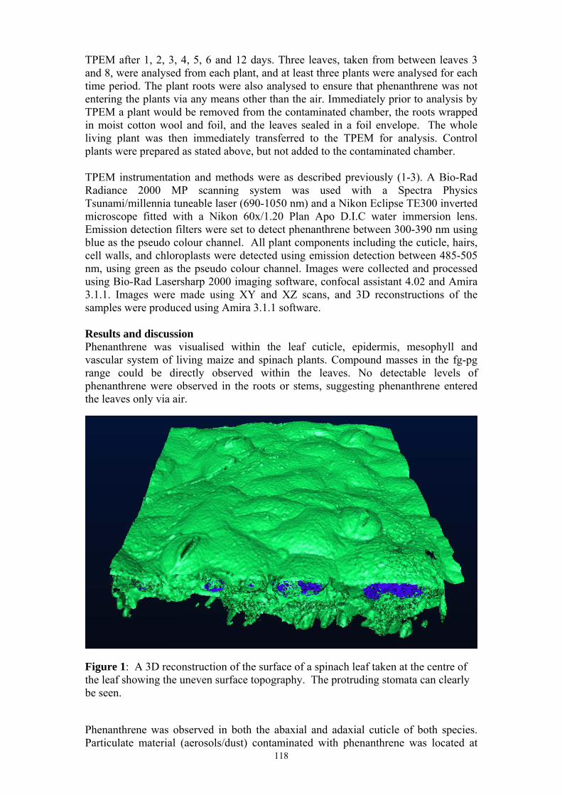
118

TPEM after 1, 2, 3, 4, 5, 6 and 12 days. Three leaves, taken from between leaves 3 and 8, were analysed from each plant, and at least three plants were analysed for each time period. The plant roots were also analysed to ensure that phenanthrene was not entering the plants via any means other than the air. Immediately prior to analysis by TPEM a plant would be removed from the contaminated chamber, the roots wrapped in moist cotton wool and foil, and the leaves sealed in a foil envelope. The whole living plant was then immediately transferred to the TPEM for analysis. Control plants were prepared as stated above, but not added to the contaminated chamber. TPEM instrumentation and methods were as described previously (1-3). A Bio-Rad Radiance 2000 MP scanning system was used with a Spectra Physics Tsunami/millennia tuneable laser (690-1050 nm) and a Nikon Eclipse TE300 inverted microscope fitted with a Nikon 60x/1.20 Plan Apo D.I.C water immersion lens. Emission detection filters were set to detect phenanthrene between 300-390 nm using blue as the pseudo colour channel. All plant components including the cuticle, hairs, cell walls, and chloroplasts were detected using emission detection between 485-505 nm, using green as the pseudo colour channel. Images were collected and processed using Bio-Rad Lasersharp 2000 imaging software, confocal assistant 4.02 and Amira 3.1.1. Images were made using XY and XZ scans, and 3D reconstructions of the samples were produced using Amira 3.1.1 software. Results and discussion Phenanthrene was visualised within the leaf cuticle, epidermis, mesophyll and vascular system of living maize and spinach plants. Compound masses in the fg-pg range could be directly observed within the leaves. No detectable levels of phenanthrene were observed in the roots or stems, suggesting phenanthrene entered the leaves only via air.

Figure 1: A 3D reconstruction of the surface of a spinach leaf taken at the centre of the leaf showing the uneven surface topography. The protruding stomata can clearly be seen. Phenanthrene was observed in both the abaxial and adaxial cuticle of both species. Particulate material (aerosols/dust) contaminated with phenanthrene was located at

119

the surface of the cuticle and became encapsulated within the cuticular waxes. Over time, diffuse areas of phenanthrene formed within the adjacent cuticle. However, most (>95%) of the phenanthrene reaching the leaves arrived via gas phase transfer. Phenanthrene was found within the wax plugs of stomata of both species and on the external surface of the stomatal pore, but not on the internal surface, or within the sub-stomatal cavity. Phenanthrene diffused through the cuticles of both species in 24-48 h, entering the epidermis to reside predominantly within the cell walls of maize (indicative of apoplastic transport) and the cellular cytoplasm of spinach (indicative of symplastic transport). Phenanthrene accumulated within the spinach cytoplasm where it concentrated into the vacuoles of the epidermal cells. Less than 10% of phenanthrene entered the cytoplasm of the maize cells. Phenanthrene entered the internal mesophyll of both species, and was found within the mesophyll cell walls, at the surface of the chloroplasts and within the cellular cytoplasm. Phenanthrene was observed within the xylem of maize following 12 days exposure. The cuticle and epidermis at the edges of spinach leaves had a systematically higher concentration of phenanthrene than the cuticle and epidermal cells at the centre of the leaf.

a b

c Figure 2: Phenanthrene within the epidermal cell walls of maize 25 μm depth (a) and epidermal cell cytoplasm and vacuoles of spinach (b-c). Organelles are shown as distinct green circles. Phenanthrene shows a diffuse distribution within the cytoplasm, concentrating within the cellular vacuole after 144 h. (b) XY image within the epidermal cell depth 26 μm, (c) XZ image through the leaf. The intense blue areas show phenanthrene concentrated within the cell vacuoles. During the 12 day uptake period, phenanthrene was observed within 9 distinct compartments as represented in Figure 3. These were: 1. sorbed to particulate matter; 2. within the cuticle; 3. within the stomatal plug; 4. within the cuticular plug; 5. within the maize cell walls; 6. within the spinach cytoplasm and 7. vacuole; 8. within the

120

mesophyll and 9. within the maize xylem. This has important implications for understanding the fate of these chemicals within plants, and for modelling the role that vegetation plays in the global cycling of these chemicals.

a.

b. Figure 3: Schematic diagrams showing the locations where phenanthrene was visualised within leaves of spinach (left of the Figure) and spinach (right) after 12 days exposure to an atmosphere contaminated with phenanthrene. Greater detail of the apoplastic and symplastic flow is shown in b. It is often assumed that persistent and lipophilic compounds just partition into plant lipids, notably the cuticle. Plant leaf models are usually structured as having one- or two-compartments with respect to such compounds. However, the uptake storage and accumulation of phenanthrene from the atmosphere to leaves of maize and spinach was not restricted to the cuticle. In fact, the results even suggested that the epidermis and mesophyll of these species displayed a greater capacity for chemical storage and accumulation than the cuticle.

121

Two compartment models generally consider a small and rapidly responding surface compartment which interacts directly with the atmosphere, and a larger (slow responding) internal storage reservoir. Indeed, experimental observations in which contaminated leaves are brought into contact with clean air and their depuration monitored have shown an initial very rapid clearance, followed by much slower (and then sometimes negligible) losses. The data obtained here generally support this notion, with the cuticle (surface compartment) filling rapidly to reach a steady state within 24-48 h in both species. Subsequent, longer-term uptake supplied the epidermis and mesophyll of maize and spinach. Presumably, the ‘internal compartment’ may incorporate the apoplast of the leaf, comprising the cell walls and intracellular spaces, or the symplast of the leaf, comprising of the internal cellular cytoplasm and vacuoles of the leaf. This study suggests that the internal (slow) reservoir of the leaf incorporates the epidermis, mesophyll and vascular system of the leaf and can be further divided into the apoplast and symplast. The apoplast includes the cell walls and intercellular spaces of the leaf and does not represent a significant volume of the leaf, while the symplast incorporates the cellular cytoplasm and vacuoles of the leaf - a large leaf volume. As Figure 3b shows, the two species studied showed very different phenanthrene distribution between these compartments. In maize, it was observed to move through and accumulate within the apoplast, while in spinach it predominantly entered the symplast. These observations may indicate different ‘internal reservoirs’, depending on species, which may have important implications for routes and rates of movement, storage location and capacity, and overall fate within the leaf. Phenanthrene travelled more rapidly and further into the maize leaf through the apoplast than in the spinach leaf through the symplast. If the same amount of compound is taken into leaves with an apoplastic or symplastic internal reservoir, it will presumably move a greater distance into the leaf with the apoplastic reservoir, because the apoplastic reservoir requires only a small amount of chemical to ‘fill’ a large volume of the leaf whilst the symplastic reservoir will require a relatively large amount of chemical to ‘fill’ a small volume of the leaf. This may help explain why phenanthrene was observed to move more rapidly into the maize mesophyll than spinach, and reached the vascular tissues in maize and not spinach. These observations highlight the importance of species differences in the uptake and storage of organic chemicals. Acknowledgements

We are grateful to the UK Natural Environment Research Council (NERC) for provision of a PhD studentship (NER/S/A2002/10394) to EW.

References 1. Wild, E., Dent, J., Barber, J.L., Thomas, G.O., Jones, K.C (2004). Environ. Sci. Technol.

38: 4195-4199. 2. Wild, E., Dent, J., Thomas, G.O., Jones, K.C. (2005) Environ. Sci. Technol. 39, 268-273. 3. Wild, E., Dent, J., Thomas, G.O., and Jones, K.C. (2005) Environ. Sci. Technol. 39,

3695-3702.

122

Annex I. List of participants.

Workshop on Persistent Organic Pollutants (POPs) in the European Atmosphere: Concentrations, Deposition and Sources in Europe

Stresa, Hotel La Palma

17/10/2005 - 19/10/2005

Speakers

KNUT BREIVIK Norwegian Institute for Air Research (NILU) P.O. Box 100 N - 2027 Kjeller Tel. :+4763898000 fax: +4763898050 E-mail: [email protected] TERRY BIDLEMAN Environment Canada Centre for Atmospheric Research Experiments 6248 CND - L0L 1N0 Egbert, Ontario Tel. :1-705-458-3322 fax: 1-705-458- E -mail: [email protected] JOEL BAKER University of Maryland Chesapeake Biological Laboratory USA - 20688 Solomons, Maryland Tel. :01-410-326-7205 fax: 01-410-326-7341 E-mail: [email protected]

EVA BRORSTRÖM LUNDEN IVL Swedish Environmental Research Institute Ltd. P.O. Box 47086 S - 40258 GÖTEBORG Tel. :+46 31 725 6200 fax: +46 31 725 6290 E-mail: [email protected] IVAN HOLOUBEK Masaryk University Kamenice CZ - 625 00 Brno tel. :+420 549 491 475 fax: +420 549 492 840 e mail: [email protected] RONALD HITES Indiana University SPEA 410 H USA - 47405 Bloomington Tel. :812-855-0193 fax: 812-855-1076 E-mail: [email protected]

mailto:[email protected]






123

STEVEN J. EISENREICH Toxicology and Chemical Substances and European Chemicals Bureau (ECB) European Commission Joint Research Centre (JRC) Institute for Health and Consumer Protection TP 582, I-21020 Ispra (VA) Italy Tel: +39-0332-78-9037 (office) Tel: +39-0332-78 97 25 (secretary) Fax: +39-0332-78 9963 Email: [email protected] JORDI DACHS CSIC Jordi Girona 18-26 E - 08034 Barcelona Tel. :+34-93-4006118 E-mail: [email protected] EURIPIDES STEPHANOU University of Crete, Environmental Chemical Processes Laboratory Knossos GR - 71409 Heraklion Tel. :+302810393628 fax: +302810393678 E-mail: [email protected] MICHAEL McLACHLAN Stockholm University Krossbacken 35 S - S--18770 Tääby Tel. :+46 8 674 7228 E- mail: [email protected] FRANK WANIA UNIVERSITY OF TORONTO AT SCARBOROUGH Department of Pysical and Environmental Sciences CND - M5R1P1 Toronto Tel. :416-287-7225 E- mail: [email protected] KEVIN JONES Lancaster University Environmental Science Department Lancaster, LA1 4 UK - LA1 4YQ Lancaster Tel. :44-1524-593972 E-mail: [email protected] JAVIER CASTRO JIMENËZ Inland and Marine Waters Unit Institute for Environment and Sustainability European Commission - Joint Research Centre (JRC) Via Enrico Fermi, 1 21020 Ispra (VA), Italy, TP 290 Tel: 0039-0332-786070 FAX: 0039-0332-786351 E-mail: [email protected] KERI HORNBUCKLE University of Iowa 4105 SC Department of Civil and Environmental Eng USA - 52242 Iowa City Tel. :319 384 0789 fax: 319 335 5660 E-mail: [email protected]









124

DEREK MUIR Environment Canada 867 Lakeshore Road CND - L7R 4A6 Burlington tel. :905-319-6921 e mail: [email protected] MARCO VIGHI Università degli Studi di Milano Bicocca Dip. di Scienze dell'Ambiente e del Territorio (DISAT) Piazza della Scienza 1 - 20126 Milano - Italy Tel: +39 02 6448 2741 Fax: +39 02 6448 2795 e-mail: [email protected] JOAN GRIMALT IIQAB-CSIC Jordi Girona E - 08034 Barcelona Tel. :+34934006122 fax: +34932045904 E-mail: [email protected] DEBORAH SWACKHAMER University of Minnesota Mayo Mail Code #807, 420 Delaware St SE USA - 55455 Minneapolis Tel. :612-626-0435 fax: 612-626-4837 E-mail: [email protected] INGRID VIVES RUBIO Inland and Marine Water Unit Institute of Environment and Sustainability (IES) European Commission - Joint Research Center Via Enrico Fermi, 1, TP 290 21020 Ispra (VA) Italy Tel. +39 0332 786639 Fax. +39 0332 786351 Email. [email protected] Other participants GABRIELE SCHOENING European Environment Agency Kongens Nytorv DK-1050 Copenhagen K Tel:+4533367265 Fax:+4533367151 E-mail: [email protected] GUNTHER UMLAUF Institute for Environment and Sustainability T.P. 290 European Commission – Joint Research Centre Via Fermi I-21020 Ispra (VA) Italy Tel.: 0039-0332-786040 Fax: 0039-0332-786351 E-mail: [email protected] JOSE MANUEL ZALDIVAR COMENGES European Commission, Joint Research Centre Institute for Environment and Sustainability, TP 272 21020 Ispra (VA), Italy tel.+39-0332-789202 fax +39-0332-785807 E-mail: [email protected]









125

SIBYLLE DUERI Inland and Marine Waters Unit Institute for Environment and Sustainability European Commission - Joint Research Centre (JRC) Via Enrico Fermi, 1 21020 Ispra (VA), Italy, TP 290 Tel: 0039-0332-786455 FAX: 0039-0332-785807 E-mail: [email protected] GENEVIEVE DEVILLER Inland and Marine Waters Unit Institute for Environment and Sustainability European Commission - Joint Research Centre (JRC) Via Enrico Fermi, 1 21020 Ispra (VA), Italy, TP 300 Tel.: ++39-0332-786692| Fax: ++39-0332-785212 E-mail: [email protected] BAREND VAN DROOGE ICER-CSIC Jordi Girona E - 08034 Barcelona Tel. :0034933258173 E-mail: [email protected] JAN WOLLGAST Inland and Marine Waters Unit Institute for Environment and Sustainability European Commission – Joint Research Centre (JRC) Via Enrico Fermi, 1 21020 Ispra (VA), Italy, TP 290 Tel.: ++39-0332-789096 Fax: ++39-0332-786351 E-mail: [email protected] MARIA HELENA ALVES MACIEL Inland and Marine Waters Unit Institute for Environment and Sustainability European Commission - Joint Research Centre (JRC) Via Enrico Fermi, 1 21020 Ispra (VA), Italy, TP 272 Tel: 0039-0332-789391 FAX: 0039-0332-789328 E-mail: [email protected] GIULIO MARIANI Inland and Marine Waters Unit Institute for Environment and Sustainability European Commission – Joint Research Centre (JRC) Via Enrico Fermi, 1 21020 Ispra (VA), Italy, TP 290 Tel.: ++39-0332-785522 Fax: ++39-0332-786351 E-mail: [email protected] ROBERT LOOS European Commission - DG Joint Research Centre Institute for Environment and Sustainability Inland and Marine Waters Unit Via E. Fermi, TP 290, Ispra (VA), I-21020, Italy Phone: +39 0332 786407 Fax: +39 0332 786351 E-mail: [email protected]








126

GEORG HANKE Inland and Marine Waters Unit Institute for Environment and Sustainability European Commission – Joint Research Centre (JRC) Via Enrico Fermi, 1 21020 Ispra (VA), Italy, TP 300 Tel.: ++39-0332-785586 Fax: ++39-0332-785212 E-mail: [email protected] MICHELA GHIANI Joint Research Centre IES-Inland and Marine Waters Unit Via E. Fermi, 1 - 21020 Ispra (VA) ITALY TP290 Phone: +39 0332 789282 Fax: +39 0332 786351 e-mail: [email protected]



127

European Commission

EUR 22876 EN – Joint Research Centre, Institute for the Environment and Sustainability Title: Persistent Organic Pollutants (POPs) in the European Atmosphere: An Updated Overview Editors: J. Castro-Jiménez, S. J. Eisenreich, and I.Vives Contributing Authors: T. Bidleman, E. Brorstrom Lunden, J. Baker, K. Breivik, J. Castro-Jiménez, J. Dachs, S. J. Eisenreich, J. Grimalt, R. Hites, I. Holubeck, K. Hornbuckle, K. Jones, G. Mariani, M. McLachlan, D. Muir, E. Stephanou, D. Swackhamer, G. Umlauf, B. L. van Drooge, M. Vighi, I. Vives, and F. Wania Luxembourg: Office for Official Publications of the European Communities 2007 – 126 pp. – 21 x 29.7 cm EUR - Scientific and Technical Research series; ISSN 1018-5593 Abstract POPs are a group of chemicals which share some specific characteristics that make them of high international concern. Due to their semivolatility, POPs present a widespread distribution being able to reach remote locations and areas after traveling long distances in the atmosphere where they have never been produced nor used. Different chemical families are considered as POPs, such as PCBs, OCPs, PCDD/Fs, PAHs, and, PCNs. In addition, some emerging contaminants are currently considered as candidate POPs, like PBDEs and PFCs. POPs exist in the atmosphere as gases and bound to particles depending on their physico-chemical properties. This affinity to gas or particulate phase is of relevant importance in the processes of POP atmospheric global transport and degradation. POPs are delivered to aquatic and terrestrial ecosystems by atmospheric deposition, air-water interchanges and direct discharges. The general hydrophobic nature of POPs results in high affinity to organic matter and biota tissues. Consequently, organisms and sediments become final “sinks” of POPs, due to the low metabolic activity for these compounds and their slow degradation processes in the environment. A number of national and international actions have been promoted to reduce or ban their production and control their emissions to the environment. The UNEP Stockholm Convention adopted in May 2001. The Artic Monitoring and Assessment Programme (AMAP) is measuring atmospheric concentrations of POPs in the artic region since it was established in 1991. At a European scale a big effort is being carried out combining the update of existing monitoring programmes with the generation of new legislations. Such is the case of the largest monitoring network across Europe gathering concentrations of POPs in air and deposition (EMEP). On the political side, the brand new European legislation on chemicals, REACH, will regulate the production of chemicals at a European scale. In addition, other POPs monitoring programmes exist at regional or national scales and a large number of “independent” sites measuring atmospheric concentrations of POPs are spread out in the European geography. Considering such a scenario it seems obvious that a strong effort in harmonization and communication of results and monitoring and research strategies needs to be achieved. A step to facilitate this needed interaction was the workshop on “Persistent Organic Pollutants (POPs) in the European Atmosphere – Concentration, Deposition and Sources in Europe –“ organized by the European Commission Joint Research Center held in October 17-19th, 2005 in Stresa (Italy). It was one of the objectives of the workshop to gather top experts from Europe and North America to share their expertise on POP monitoring and research in the atmospheric compartment in order to evaluate their current status in Europe. Invited experts develop their professional activities either in the existing POPs monitoring networks or in research institutions closely linked to POPs research (Annex I). Other objectives of the workshop were to

128

explore future research lines on the topic and to establish links with the existing science and new policies in Europe regarding chemicals. Twenty oral communications were presented covering relevant key issues on POPs: In this report a compilation of the extended abstracts submitted by the participants is presented, whereas the working result output of the workshop will be submitted as an article to a peer-reviewed scientific journal.

129

The mission of the JRC is to provide customer-driven scientific and technical support for the conception, development, implementation and monitoring of EU policies. As a service of the European Commission, the JRC functions as a reference centre of science and technology for the Union. Close to the policy-making process, it serves the common interest of the Member States, while being independent of special interests, whether private or national.

Persistent Organic Pollutants (POPs) in the European...

Documents

Transcript of Persistent Organic Pollutants (POPs) in the European...