Persistence of Business Cycles in MultisectorRBC Models∗

Jess BenhabibDepartment of EconomicsNew York University

Roberto PerliDivision of Monetary AffairsFederal Reserve Board

Plutarchos SakellarisDepartment of Economics

Athens University of Economics and Business

August 24, 2005

Abstract

In this paper we explore whether the changing composition of out-put in response to technology shocks can play a significant role in thepropagation of shocks over time. For this purpose we study two mul-tisector RBC models, with two and three sectors. We find that, whilethe two sectors model requires a high intertemporal elasticity of sub-stitution of consumption to match the various dynamic properties ofU.S. macroeconomic data, the three sector model has a strong prop-agation mechanism under conventional parameterizations, as long asthe factor intensities in the three sectors are different enough.

Key Words: Real Business Cycles, PersistenceJEL Classification: E00, E3, O40.

∗Address for correspondence: Jess Benhabib, Dept. of Economics, New York University,New York, NY 10003. We would like to thank Susanto Basu, Michele Boldrin and RichardRogerson for helpful comments and discussions. Technical support from the C. V. StarrCenter for Applied Economics is gratefully acknowledged.

1

1 Introduction

Over the past several years, attention has been drawn to the fact that stan-dard one sector, stochastic optimal growth models–the paradigm of RBCtheory–do not have a strong enough endogenous mechanism to propagateshocks over time. As a consequence, these models are not capable of gener-ating persistent business cycles.1 The purpose of this paper is to show thatmultisector models have a potentially strong propagation mechanism whichdoes not rely upon any extra features.We identify the presence of a strong propagation mechanism with a

hump—shaped impulse response of output growth, i.e., with the presenceof a strong trend—reverting component; with an autocorrelation function ofoutput growth which is significantly positive for at least three lags, as itseems to be in the U.S. data; and with a power spectrum of output growthwhich has a peak at business cycle frequencies, again as it is the case inthe U.S. data.2 Cogley and Nason, [11], have shown that the standard RBCmodel has a monotonically decreasing impulse response function of output toa non—permanent shock, an autocorrelation function of output growth whichis always very close to zero and possibly negative, and a flat spectrum ofoutput growth.Several modeling strategies are known to mitigate the problem: quadratic

adjustment costs to capital and labor, as in Cogley and Nason, [11]; variablefactor utilization rates, as in Burnside and Eichenbaum, [10]; variable factorutilization rates within an efficiency wages framework, as in Beaudry andDevereaux, [5]; the embedding of a search—theoretic approach to the labormarket within an otherwise standard RBC model, as in Andolfatto, [1]; habitformation in leisure coupled with increasing returns to scale, as in Wen, [18];home production with enough productive externalities to generate multipleequilibria, as in Perli, [15]; sector-specific externalities, as in Benhabib andFarmer, [8]; the addition of a human capital sector with low elasticity of

1This fact was pointed out, for example, by Cogley and Nason, [11], and Rotembergand Woodford, [17].

2We follow the same definition of propagation mechanism given in Cogley and Nason,[11]; as consequence we feed strongly autocorrelated shocks to our models. Alternatively,we could have looked at the autocorrelation and spectra of levels, rather than growth rates,and have fed white noise shocks to the models. This is the approach taken by Beaudryand Devereaux, [5].

2

substitution between raw labor and human capital, as in Perli and Sakellaris,[16]; and human capital with variable factor utilization rates, as in DeJonget al., [12].All the previous papers essentially try to break the post-impact inverse

relationship between consumption and labor of a non—permanent shock.3

While in the period of impact consumption, labor and output may all movein the same direction, after the impact the intratemporal marginal efficiencycondition, which has to be satisfied in any one sector RBC model, forcesconsumption and labor to move in opposite directions. Since consumptiontypically continues to increase after a positive shock, labor decreases forcingoutput to decrease as well, unless capital responds extremely strongly.4 Thepapers mentioned above that rely on adjustment costs or variable factorutilization rates or search, [11], [10], [5], [1], [12], introduce a delay in theresponse of labor to the technology shock, whereas the other papers, [18], [15],[16], [8], try to modify the working of the intratemporal marginal efficiencycondition, to allow consumption and labor to move in the same direction fora few periods after impact.In a more recent paper, Gali [13] decomposes the shocks into a technol-

ogy and non—technology component. Using VARs he demonstates that, inresponse to a technology shock, hours may decline on impact and in factinduce a negative correlation between productivity and hours. Indeed, in re-sponse to a technology shock, “the initial increase in labor productivity andthe (smaller) increase in output is reflected in a short-lived, though persis-tent (and significant), decline in hours.”5 Gali suggests that this is compatiblewith a model of sticky prices, so that an increase in productivity does notlead to a sufficient rise in output and sales, and therefore must be reflectedin a curtailment of hours. Basu, Fernald and Kimball [4], in a model of firmswith quasi-fixed inputs and variable capacity utilization, also find that inresponse to a technology shock input use and the output of non-residentialinvestment decline, and argue that this provides evidence in favor of stickyprice models.In this paper we pursue a different strategy: instead of adding extra fea-

3We assume in what follows that the shocks are always strongly autocorrelated, but donot contain a unit root.

4For a detailed discussion of this problem see Perli, [15], and Perli and Sakellaris, [16],who, in turn, build on the early paper by Barro and King, [2].

5See Gali [13], p. 259, and Figure 3, p. 262.

3

tures to a one sector model, we explore the propagation behavior of twomulti—sector models. Our idea is that looking at the composition of outputmay also help understanding the way shocks are propagated in the economy.While in one sector models output is defined simply as the output of a singleproduction function, in multi-sector models output is the result of the com-position of consumption and investment goods, i.e., Yt = Ct +

Pni=1 pitXit.

Thinking in terms of impulse response functions, it is clear that output candisplay a hump—shaped pattern in response to a shock even if neither the con-sumption good nor the investment goods have a hump—shaped response, or ifonly one of them has it. In the case of a two sector model, for example, outputcould have the appropriate impulse response if, after the impact of a posi-tive shock, consumption increases more than what investment decreases. Inparticular, we confine our attention to a one—capital—good, two—sector modeland a two—capital—goods, three—sector model. We show that the latter hasa strong endogenous propagation mechanism for a wide range of empiricallyplausible parameters, as long as the three sectors have sufficiently differentfactor intensities. The one—capital—good, two—sector model, on the otherhand, requires the strong additional assumption of a very low intertemporalelasticity of substitution of consumption to generate artificial data with thesame dynamic properties as the real U.S. data. It is nonetheless useful toexamine the behavior of this model since it is easier to grasp the intuitionbehind the persistence results within its simpler structure. In particular, weshow that composition effects not only can produce the hump-shaped impulseresponses observed in the data, but also can explain the impulse responsesgenerated by Gali, [13], and “the fact that the bulk of the joint variation inemployment and productivity arising from a technology shock takes place onimpact, with both variables moving in opposite directions."6

The paper is organized as follows: the next section discusses the one—capital—good, two—sector model; section 3 discusses the two—capital—goods,three—sector model; and section 4 concludes.

6See Gali, [13], p. 259.

4

2 A Two—Sector Model

In this section we consider a standard model with a single capital good andtwo sectors, consumption and investment. The representative agent chooseshow to allocate capital and labor across the two sectors in order to maxi-mize the discounted sum of each period utilities, subject to the productionconstraints in the two sectors and the law of motion of capital and of thetechnologies. Formally:

maxKCt ,LCt ,LIt

E0Xt

ρt∙C1−σt

1− σ+ θ

(1− LCt − LIt)1−γ

1− γ

¸subject to:

Ct = qCzCtKαCtL

1−αCt

Xt = qXzXtKβXtL1−βXt

Kt+1 = (1− δ)Kt +Xt

zCt+1 = zξCtet

zXt+1 = zζXtut

Kt = KCt +KXt

To solve this problem, we substitute the produciton function for Ct into theutility function; the first order conditions with respect to KC , LC , and LI

are, respectively:

MUCt ·MPKCt = ρE∂vt+1∂Kt+1

·MPKXt (1)

MUCt ·MPLCt = MULCt (2)

MULXt = ρE∂vt+1∂Kt+1

·MPLXt (3)

where MPw and MUw denote the marginal product and marginal utility,respectively, of variable w and vt+1 is the value function at time t + 1. Tofind an expression for E(∂vt+1/∂Kt+1) consider that:

∂vt∂Kt

= ρE∂vt+1∂Kt+1

(1− δ +MPKXt) (4)

5

From (1):

ρE∂vt+1∂Kt+1

=MUCt ·MPKCt

MPKXt

and therefore, substituting into (4) and updating one period :

E∂vt+1∂Kt+1

=MUCt+1 ·MPKCt+1

MPKXt+1

· ¡1− δ +MPKXt+1

¢(5)

The model has to be solved numerically; to this end, we use a log—linearization around the steady state. We can thus write the system asfollows: ⎛⎜⎜⎝

bKt+1bLCt+1bzCt+1bzXt+1

⎞⎟⎟⎠ = J ·

⎛⎜⎜⎝bKtbLCtbzCtbzXt

⎞⎟⎟⎠+Q ·µ

etut

¶(6)

where J is the Jacobian matrix and bw indicates the percentage deviationof variable w from its steady state. All other variables can be expressed as(approximately) linear functions of total capital, labor in the consumptionsector, and the two shocks. System (6) can be simulated numerically; ofcourse, an appropriate value of bLC must be chosen at any point in time as afunction of bK, bzC and bzX since the model has a unique equilibrium.Once we simulate artificial time series for all the variables we must com-

pute output. One way to do it is to write:

Yt = Ct + ptXt

where pt is the price of the investment good in terms of the consumptiongood. We can obtain pt from the static first order conditions of the firmswith respect to capital, MPKCt = rt, and ptMPKXt = rt. Dividing one bythe other we get:

pt =MPKCt

MPKXt

i.e., the price of the investment good is equal to the ratio of the mar-ginal product of capital in the two sectors. The same relation could havebeen obtained using the first order conditions with respect to labor. Output

6

computed in this way would correspond to “nominal” output, since currentprices are used. Alternatively, one could use Yt = Ct + p ∗ Xt, where p∗ isthe steady state value of the price level and also the starting point in oursimulation. This would correspond to “real output”, expressed in terms ofprices at time zero.

2.1 Calibration and Results

We calibrate some of the parameters in a standard way, and we choose theremaining ones so that the model exhibits a degree of persistence of theshocks compatible with what we observe in the U.S. data. We then askthe question of whether the latter values are plausible or not in view of theavailable empirical evidence.We set the depreciation of capital, δ, to 0.025 and the discount factor,

ρ, to 0.9898, since we want to simulate quarterly data. Moreover, as it isstandard in the RBC literature, we assume that the utility function is linearin leisure, i.e., we set γ = 0. We then set θ = 1.51 so that, in the steadystate, the number of hours worked is 1/3 of the total time available. Finally,we assume that the shocks to both sectors are highly persistent; in particularwe set ξ = ζ = 0.95.We choose the remaining parameters, α, β, and σ, in order for the model

to have a significant endogenous propagation mechanism. We provide anintuition for two cases under which endogenous persistence arises. As notedin the introduction, persistence can arise in this model due to changes in thecomposition of output. Note that we say that we have persistence when theimpulse response of output is “hump shaped”, i..e., when output increaseswhen a positive, non permanent shock first hits the economy, and contin-ues to increase for a few periods after that. Since output is composed ofconsumption and investment, this can happen if both variables continue toincrease after the impact of the shock; but it can also happen if one of thetwo variables increases more than the other decreases. Below we present acase in which the latter possibility occurs.Suppose that both sectors are subject to the same technology shocks, i.e.,

that et and ut are identical.7 Assume that a positive, persistent shock hits

7The same results that we report below hold also for different innovations, as long asthey are strongly positively correlated.

7

both sectors. If households like to smooth consumption, we will typicallyobserve that both consumption and investment increase at impact, and thendecrease monotonically; this clearly is not going to generate any persistencein output. Things could be different, however, if households are not too con-cerned about consumption smoothing, i.e., if the utility of consumption islinear or close to linear. If that is the case, the higher interest rate inducedby the positive shock provides a strong incentive for households to substitutefuture consumption for present consumption; indeed, with very little curva-ture of the utility function, households reduce consumption at date zero, theperiod of impact. Conversely, investment strongly increases–more so thanconsumption declines–so output increases at date zero. In the periods afterthe shocks have hit the economy, however, households will start consumingmore (the consumption they deferred at date zero), and investment will startdeclining. Given its low intertemporal elasticity of substitution, and giventhe high elasticity of the labor supply that we assume (γ = 0), consumptionactually increases faster than investment decreases, and therefore outputkeeps increasing. Eventually, both consumption and investment will go backto their steady states, and so output has to start decreasing and go back toits steady state after a few periods. But, since at least initially C increasesfaster than pX decreases, output has a hump—shaped impulse response andtherefore the model has a strong endogenous propagation mechanism.The first restriction that we have to impose to our remaining parameters,

therefore, is that σ has to be low; we choose σ = 0.07, the higher value thatgives the desired persistence result. Note, moreover, that we can not have alow labor supply elasticity: if γ is high, total labor is practically constant, andthe only movements in labor that we see are between the two sectors. Theseintersectoral movements are simply not sufficient to push up consumptionenough to generate noticeable persistence; we need some extra labor goingto the consumption sector from leisure after the impact of the shock. A linearutility of leisure is standard in RBC models. We view an almost linear utilityof consumption however as a significant difficulty for the model above, andwill address and correct it in the three—sector model in the next section.Those on σ and γ are the only restrictions that we need in order to

achieve persistence. We want, however, to calibrate the model so that notonly persistence, but also other statistics are in line with what we observe inthe data. For example, if the factor intensities are identical in the two sectors,

8

consumption remains below the steady state for several periods after impact;this has the unpleasant implication of making consumption weakly correlatedwith output, or even countercyclical, depending on parameter values.8 Theproblem can be easily corrected assuming that the investment sector is morecapital intensive than the consumption sector, i.e., that β > α. In particularwe choose α = 0.2 and β = 0.4, although the same results below would beobtained with many other different combinations; what matters is the ratio ofthe two capital shares. In this way, after impact, labor will tend to move backfaster to the consumption sector, which is labor intensive, and consumptionoutput will respond more strongly and rapidly to the inflow of labor. Withthis calibration consumption is below its steady state only for the period ofimpact, which implies a much higher correlation with output.

Y C X L KStandard Deviation 1.00 0.94 4.52 0.93 0.41

(1.00) (0.49) (2.82) (0.86) (0.34)Correlation with Output 1.00 0.72 0.66 0.99 0.44

(1.00) (0.76) (0.96) (0.86) (0.14)AR(1) Coefficient 0.75 0.76 0.66 0.75 0.97

(0.90) (0.84) (0.76) (0.90) (0.96)Table 2.1 (U.S. Data in parenthesis)

The standard RBC set of statistics for several variables is in Table 2.1.We see that the model performs more or less like other RBC models, i.e., itcaptures several “static” aspects of the U.S. business cycle quite well. Thebiggest problem, however, is that consumption is almost twice as volatile asin the U.S. data; this was obviously to be expected, given the extremely highintertemporal elasticity of substitution of consumption that we assumed.

The performance of the model in terms of persistence is shown in figures1—3. The impulse response function of output is shown in figure 1; withrespect to the impulse response of U.S. output, we see that Y takes too long

8If the factor intensities are equal in the two sectors, and the shocks are the same, themodel is equivalent to a one—sector model. The one—sector model, therefore, can exhibitpersistence if the utility of consumption is very flat. The problem is not only that thisassumption is quite unrealistic; standard RBC statistics are also quite off the mark in thatcase.

9

Figure 1: Impulse Response

10

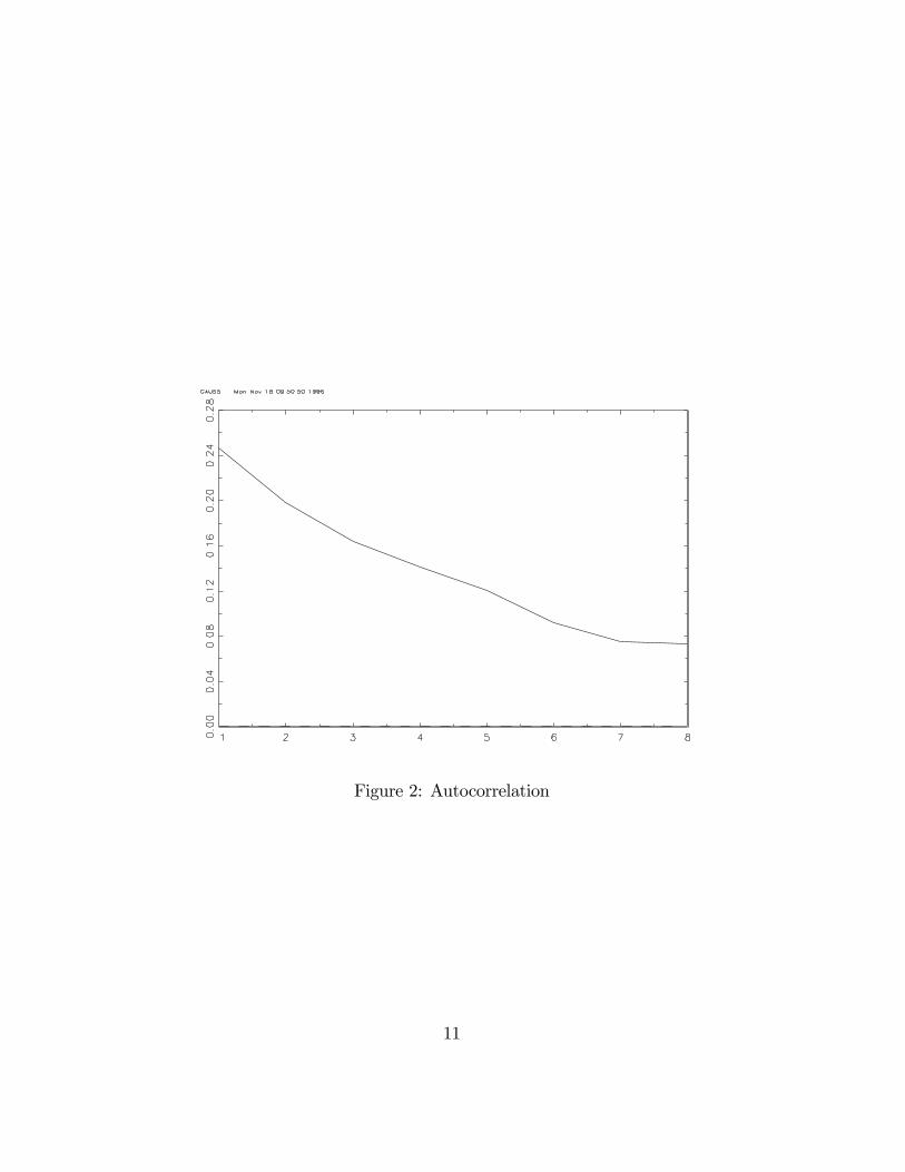
Figure 2: Autocorrelation

11

Figure 3: Power spectrum of output growth: two—sector model

12

to go back to its steady state, a sign that our model has too much, rather thantoo little persistence. Figure 2 shows the first ten lags of the autocorrelationfunction of output growth; they are all positive, which is another sign of toomuch persistence relative to the U.S. data. Finally, figure 3 shows the powerspectrum of output growth; the presence of a peak is clear, although it occursat frequencies slightly lower than the typical business cycle frequencies; thisagain says that the model has too much persistence.While with the parameterization above we are able to obtain a degree

of persistence comparable to, and actually higher than, what is observedin the U.S. data, we have the problem that the intertemporal elasticity ofsubstitution of consumption has to be too high. In the next section we showthat a three—sector model can produce the same level of persistence with amore conventional logarithmic utility of consumption.

3 A Three—Sector Model

In the previous section we showed that a two sector model can generate per-sistence of technology shocks comparable to what we observe in the U.S. dataif consumption increases faster than investment decreases for a few periodsafter the impact of a positive technology shock. This required, however, avery high intertemporal elasticity of substitution of consumption. The ideaof this section is to have a second investment good to absorb some of the roleplayed by consumption in the two sector model. Here we assume a conven-tional intertemporal elasticity of substitution of consumption equal to one,and we introduce a second investment sector, which we denominate W. Themodel therefore has one consumption good and two capital goods. Even ifhere consumption does not react very strongly to technology shocks, as itappears to be the case in the U.S. data, the two investment goods are gen-erating persistence according to a mechanism similar to that described insection 2.The working of the three—sector model is standard: as in the previous sec-

tion, the representative agent chooses how to allocate capital and labor acrossthe three sectors in order to maximize the discounted sum of each period’sutilities, subject to the production constraints in the three sectors, the lawsof motion of the capital stocks, and the laws of motion of the technologies.Formally:

13

maxKCt ,LCt ,LIt

E0Xt

ρt∙C1−σt

1− σ+ θ

(1− LCt − LIt)1−γ

1− γ

¸subject to:

Ct = qCzCtLα0CtKα1

XCtK1−α0−α1

WCt

Xt = qXzXtLβ0XtK

β1XXt

K1−β0−β1WXt

Wt = qWzWtLγ0WtK

γ1XWt

K1−γ0−γ1WWt

KXt+1 = (1− δ)KXt +Xt

KWt+1 = (1− δ)KWt +Wt

zCt+1 = zξCtet

zXt+1 = zζXtut

zWt+1 = zηWtvt

KXt = KXCt +KXXt +KXYt

KWt = KWCt +KWXt +KWWt

Total real output is again defined as Yt = Ct + pXtXt + pWtWt, where pXand pW are the prices of the two capital goods in terms of the consumptiongood, and are computed in the same way as with the two—sector model; totalinvestment is It = pXtXt + pWtWt. The representative agent chooses howmuch to work and how much capital to use in the three sectors; total capitalis just the sum of the capital stocks used in the individual sectors. The firstorder conditions of this problem can be written as:

14

MUCt ·MPLCt = MULCt

MULXt = ρE∂vt+1∂KXt+1

·MPLxt

MULWt = ρE∂vt+1∂KWt+1

·MPLWt

MUCt ·MPKXCt = ρE∂vt+1∂KWt+1

·MPKXWt

ρE∂vt+1∂KXt+1

·MPKXXt = ρE∂vt+1∂KWt+1

·MPKXWt

MUCt ·MPKWCt = ρE∂vt+1∂KWt+1

·MPKWWt

ρE∂vt+1∂KXt+1

·MPKWXt = ρE∂vt+1∂KWt+1

·MPKWWt

where the two derivatives of the value function next period are given by:

E∂vt+1∂KXt+1

=MULXt+1

MPLXt+1

· ¡1− δ +MPKXXt+1

¢E

∂vt+1∂KWt+1

=MUCt+1 ·MPKWCt+1

MPKWWt+1

· ¡1− δ +MPKWWt+1

¢Like the two—sector model, this model cannot be solved analytically. We

solve it numerically using the same technique as above, i.e., we linearizethe Euler equations around the steady state. Since we have now two statevariables (the two capital stocks) plus three shocks, the resulting linearizeddynamical system consists of seven difference equations in seven variables(the two states, two controls, and the three shocks):⎛⎜⎜⎜⎜⎜⎜⎜⎜⎜⎝

bKXt+1bKWt+1bLXt+1bLWt+1bzCt+1bzXt+1bzWt+1

⎞⎟⎟⎟⎟⎟⎟⎟⎟⎟⎠= J ·

⎛⎜⎜⎜⎜⎜⎜⎜⎜⎜⎝

bKXtbKWtbLXtbLWtbzCtbzXtbzWt

⎞⎟⎟⎟⎟⎟⎟⎟⎟⎟⎠+Q ·

⎛⎝ etutvt

⎞⎠

15

All the other choice variables can be expressed in terms of the above variablesusing the first order conditions. Appropriate values of bLXt and bLWt have tobe chosen in every period to make sure that the transversality conditionsare satisfied, i.e., to make sure that the dynamics takes always place on thestable branch of the saddle point.

3.1 Calibration and Results

The model is calibrated using the same strategy as in the previous section, Inparticular, we set the depreciation of capital, δ, to 0.025, the discount factor,ρ, to 0.9898, and the inverse of the labor supply elasticity, γ, to zero.We setθ = 1.73, so that, again, total hours worked in the steady state are 1/3 ofthe total time available. Unlike the previous case we also set σ = 1, whichimplies that the utility is logarithmic in consumption, a standard featureof RBC models. We further assume that the shocks to all three sector arehighly persistent, ξ = ζ = η = 0.95, and identical.The factor shares are set in order to get the desired persistence and ac-

ceptable results in terms of other types of statistics. As it turns out, there areseveral combinations of parameter values that yield relatively good results.One such case involves assuming that the consumption sector is relativelylabor intensive, and that the investment sector W is relatively more capital—W intensive than the investment sector X. For example figures 4, 5 and 6and Table 3.1 below were obtained with the following parameters: α0 = 0.58,α1 = 0.32; β0 = 0.56, β1 = 0.24; γ0 = 0.39, γ1 = 0.12.

Y C I L KStandard Deviation 1.00 0.70 3.23 1.22 0.65

(1.00) (0.49) (2.82) (0.86) (0.34)Correlation with Output 1.00 0.34 0.88 0.74 0.29

(1.00) (0.76) (0.96) (0.86) (0.14)AR(1) Coefficient 0.93 0.93 0.85 0.82 0.75

(0.90) (0.84) (0.76) (0.90) (0.96)Table 3.1 (U.S. Data in parenthesis)

As one can see in figure 4, the impulse response function to a singleaggregate technology shock hitting all three sectors simultaneously is clearly

16

Figure 4: Impulse Response

17

Figure 5: Autocorrelation

18

Figure 6: Power spectrum of output growth: three— sector model

19

hump—shaped and the autocorrelation function of output growth in figure 5is always positive for the first 10 lags, a sign that, like in the previous section,we have too much, rather than too little, persistence. The results of Table3.1 are similar to those in Table 2.1 for the two—sector model, with somedifferences in the properties of consumption. As was to be expected, C isnow less volatile than before, since σ is smaller; the reduction in consumptionvolatility, however, came at the expense of an increased labor volatility. Inaddition, consumption is now only mildly procyclical.The reason why we have persistence for the plausible parameter values we

chose has again to do with the changing composition of output. When a pos-itive shock hits all three sectors with the same intensity at date zero, we seeagain that consumption still slightly decreases, but very little in percentageterms. The two investment goods, however, respond much more strongly;in particular X increases and W decreases. Since X increases more thanwhat the combined decrease in C and W , the impulse response of output tothe shock is positive at date zero. Note that here consumption decreases atimpact even if its intertemporal elasticity of substitution is not high as inthe two—sectors model; this happens because the response of the investmentgoods to the shock is very pronounced; the resulting higher real interest rateprovides an incentive to postpone consumption which is so strong that it over-comes households’ natural predisposition for sonsumption smoothing. Afterthe impact of the shock, we see that consumption and the second investmentgood, W , start increasing, while X starts decreasing. Again, the key hereis that W and C increase more than X decreases, and therefore total out-put continues to increase. This lasts for several periods, and consequentlyoutput has the pronounced hump that is the characteristic of persistence.Note that we are exploiting the same effects that yielded persistence in thetwo—sector model when the investment sector was relatively capital intensive.Only, here we do not need a high intertemporal elasticity of substitution ofconsumption, thanks to the extra reallocation of resources across the twoinvestment sectors. In other words, here one of the two investment sectors,W in particular, plays part of the role that was played by consumption inthe two—sector model.For this mechanism to work, investment goodW must be countercyclical

(or a lagging, rather than a leading, sector), and very volatile. Empirically itseems more plausible that the output of an investment sector, rather than the

20

output of the consumption sector, is more volatile than output and counter-cyclical .9 The fact that investment goodW is countercyclical (its correlationwith output is -0.41) does not of course mean that total investment is alsocountercyclical. Since the other investment good, X, is strongly procyclical,total investment is indeed procyclical, as shown in table 3.1.The particular parameter values that we chose are not the only ones that

give persistence. Simulations show that there is a wide region in the para-meter space that yields results equivalent to those shown above. This regionis characterized by the fact that the factor intensities in the three sectorshave to be sufficiently different. If the they are too close to each other, con-sumption will be countercyclical consumption. Unlike the two sector model,it is also possible that some parametrizations lead to a negative response ofoutput to the shocks; this happens when the decline in the production ofgood W is too strong.Another interesting feature of this model is its ability to magnify ex-

tremely small shocks. To generate artificial time series for output that havethe same variance of the real U.S. output we need shocks in each sector witha standard deviation of only 0.00023. Altogether, the three shocks have astandard deviation which is about 10 times smaller than what is requiredby other standard one—sector RBC models. Although we do not pursue thisargument here any further, multisector models seem therefore to be inter-esting not only for their intrinsic propagation mechanism, but also for theiramplification mechanism.We now turn to a slightly different calibration of our three-sector model

to explore the results on the negative impact response of labor hours totechnology shocks, obtained by Gali, [13] and by Basu, Fernald and Kimball[4]. The instantenous utility function is specified as above, but now we setσ = γ = 1, implying that the labor supply elasticity is also equal to 1. Weset the quarterly discount factor to ρ = 0.99 and the quaterly depreciationrate to δ = 0.025. Technology is specified as before, with the persistenceparameters for the shocks set as ξ = ζ = η = 0.95 and the standard deviationof the innovations to the normally distributed, zero mean sectoral technologyshocks to 0.0039. The Cobb-Douglas exponents for the production functionsare α0 = 0.10, α1 = 0.80; β0 = 0.97, β1 = 0.02; γ0 = 0.74, γ1 = 0.06. This

9One could interpret the output of the W sector as human capital, making its counter-cyclicality more natural.

21

specification for technology represents a strong curvature in the productionpossibility frontier, reflected in the significant differences of the Cobb-Douglasexponents across sectors10 and implies that it is quite costly to reallocatefactors across sectors.The calibration results for the model are in Table 3.2. While the match

is reasonable, consumption is too smooth relative to output, and aggregateinvestment (aggregated through relative prices) is less volatile than in thedata, although the individual sectoral components of investment and outputcould be more volatile.

Y C I LStandard Deviation 1.00 0.50 2.20 0.79

(1.00) (0.49) (2.82) (0.86)Correlation with Output 1.00 0.56 0.96 0.84

(1.00) (0.76) (0.96) (0.86)AR(1) Coefficient 0.96 0.99 0.95 0.93

(0.90) (0.84) (0.76) (0.90)Table 3.2 (U.S. Data in parenthesis)

We now turn to the impulse response functions, again with an aggregativetechnology shock hitting all three sectors simultaneously, and depicted infigure 7. As suggested by Gali [13] labor hours exhibit a pronounced declineat the impact of the technological shock, while output, consumption andinvestment exhibit the standard hump-shaped response. Note that, as inGali [13] and Basu, Fernald and Kimball [4], hours initially fall below thesteady state level, but overshoot the steady state and then converge backto the steady state level from above. Of course output and investment arevalues aggregated by contemporaneous relative prices, so sectoral "physical"output levels may not all be procyclical. Nevertheless the multisector modelgenerates the impulse responses in the data, with a negative response oflabor hours to technology shocks through compositional effects, but withoutinvoking sticky prices.Finally, we should note that our multisector approach has a close con-

nection to the recent works of Beaudry and Portier, [6] and [7], who proposeto study the impulse responses and the procyclicality of output variables in

10A specification similar in spirit would postulate significant adjustment costs in thereallocation of factors accross sectors. Such a specification prevents the excessive volatilityof factor movements and therefore of sectoral outputs. For an adjustment cost treatmentsee Huffman and Wynne [14].

22

Figure 7: Impulse Responses: Output, Consumption, Investment and Labor

23

response to news about future but not contemporaneous shocks. In such asetup, the output expansion cannot rely on the increased capacity providedby a contemporaneous technology shock, so it must either be driven by astrong and positive labor supply response, or a countercyclical sector likehome production, or complementarities and externalities in production. Thelatter has been explored by Benhabib and Nishimura ([9]) in a three sectormodel, where the positive news are represented by sunspots and thereforeoperate under full rational expectations11. The precise conditions on disag-gregated technology that will permit business cycle fluctuations consistentwith macroeconomic data in response to non-technology shocks will requirefurther work and analysis.

4 Conclusion

In this paper we presented two multisector real business cycle models and ex-plored their implications for the propagation of shocks over time. We foundthat both models, and the three—sector, two—capital—goods model in partic-ular, are able to generate artificial data with the same degree of persistenceobserved in the U.S. data. The models are also able to match several otherkey business cycle statistics to a degree similar to other standard one sectormodels. The message that we think is coming out clearly from our analysis isthat compositional effects play a significant role in the dynamic properties ofaggregate economic variables. In particular, sectoral reallocations of produc-tive factors in response to productivity shocks may be one of the fundamentalreasons why we see shocks that have persistent effects on U.S. output.

References

[1] D. Andofatto: Business Cycles and Labor Market Search. AmericanEconomic Review, vol. 86 no. 1, pp. 112—132, 1996.

11As argued in Basu and Fernald [3] however, obtaining estimates of returns to scaleand the size of external effects in the context of a multi-sector model subject to factorreallocations and compositional effects raises many difficulties and complications.

24

[2] R. Barro and R. King: Time-Separable Preferences and Intertempo-ral Substitution Models of Business Cycles. Quarterly Journal of Eco-nomics, pp. 817-839, 1984.

[3] Basu, N. and Fernald, J.: Returns to Scale in U.S. Production: Es-timates and Implications, Journal of Political Economy, vol. 105, pp.249-283, 1997.

[4] Basu, N., Fernald, J. and M. Kimball: Are Technology ImprovementsContractionary? NBER working paper 10592, NBER, Cambridge, 2004.

[5] P. Beaudry and M. Devereux: Towards an Endogenous PropagationTheory of Business Cycles. Manuscript, University of British Columbia,1995.

[6] P. Beaudry & F. Portier: An Exploration into Pigou’s Theory of Cycles, Journal of Monetary Economics, vol. 51, pp. 1183-1216, 2004.

[7] P. Beaudry and F. Portier: When Can Changes in Expectations CauseBusiness Cycle Fluctuations in Neo-Classical Settings?, NBER WorkingPapers 10776, National Bureau of Economic Research, Inc.,2004.

[8] J. Benhabib and R. Farmer: Indeterminacy and Sector-Specific Exter-nalities. Journal of Monetary Economics, vol. 37, pp. 421-443, 1996.

[9] J. Benhabib and K. Nishimura: Indeterminacy and Constant Returns,Journal of Economic Theory, 81 pp. 58-96, 1998.

[10] C. Burnside and M. Eichenbaum: Factor Hoarding and the Propagationof Business Cycle Shocks. NBER working paper no. 4675, 1994.

[11] T. Cogley and J.M. Nason: Output Dynamics in Real Business CycleModels. American Economic Review, vol. 85 no. 3, pp. 492—511, 1995.

[12] D. DeJong, B. Ingram, Y. Wen, and C. Whiteman: Cyclical Implicationsof the Variable Utilization of Physical and Human Capital. Manuscript,University of Iowa, 1996.

[13] J. Gali: Technology, Employment, and the Business Cycle: Do Tech-nology Shocks Explain Aggregate Fluctuations? American EconomicReview, vol. 89 no. 1. pp. 249—271, 1999.

25

[14] Huffman, G. W. and Wynne, M. A.,“The Role of Intertemporal Ad-justment Costs in a Multi-Sector Economy,” Journal of Monetary Eco-nomics, Volume 43, Issue 2 , April 1999, pp. 317-350 .

[15] R. Perli: Indeterminacy, Home Production and the Business Cycle: ACalibrated Analysis. Journal of Monetary Economics, vol. 41, pp. 105-25, 1998.

[16] R. Perli and P. Sakellaris: Human Capital Formation and Business CyclePersistence. Journal of Monetary Economics, vol. 42), pp. 67-92, 1998.

[17] J. Rotemberg and M. Woodford: Real— Business—Cycle models and theforecastable movements in output, hours and consumption. AmericanEconomic Review, Vol. 86 no. 1, pp. 71—89, 1996.

[18] Y. Wen: Can a Real Business Cycle Model Pass the Watson Test? Jour-nal of Monetary Economics, vol. 42, pp. 185—203, 1998.

26