PERMIX A Platform for Multiscale...

PERMIX

A Platform for Multiscale Modelling

Hossein Talebi

Institute of Structural Mechanics (ISM)

Bauhaus University–Weimar, 2012

TABLE OF CONTENTS

CHAPTER 1 Manual . . . . . . . . . . . . . . . . . . . . . . . . . . . . . . . . . . . 1

1.1 Introduction . . . . . . . . . . . . . . . . . . . . . . . . . . . . . . . . . . . 1

1.1.1 What is PERMIX . . . . . . . . . . . . . . . . . . . . . . . . . . . . . 1

1.1.2 Citing PERMIX . . . . . . . . . . . . . . . . . . . . . . . . . . . . . . 1

1.1.3 Features . . . . . . . . . . . . . . . . . . . . . . . . . . . . . . . . . . 1

1.2 Acknowledgement of the External Libraries, Codes and References . . . . . 2

1.3 Getting Started . . . . . . . . . . . . . . . . . . . . . . . . . . . . . . . . . . 4

1.3.1 Building PERMIX . . . . . . . . . . . . . . . . . . . . . . . . . . . . . 4

1.3.2 Preliminaries . . . . . . . . . . . . . . . . . . . . . . . . . . . . . . . . 4

1.3.3 Running PERMIX . . . . . . . . . . . . . . . . . . . . . . . . . . . . . 7

1.3.4 Command-line Options . . . . . . . . . . . . . . . . . . . . . . . . . . 7

1.3.5 Viewing Results . . . . . . . . . . . . . . . . . . . . . . . . . . . . . . 7

1.3.6 Jump Start Tutorial . . . . . . . . . . . . . . . . . . . . . . . . . . . . 8

CHAPTER 2 PERMIX Scripting Commands . . . . . . . . . . . . . . . . . . . . . 12

2.1 $end permix input . . . . . . . . . . . . . . . . . . . . . . . . . . . . . . . . 12

2.2 $include . . . . . . . . . . . . . . . . . . . . . . . . . . . . . . . . . . . . . . 12

CHAPTER 3 Keywords . . . . . . . . . . . . . . . . . . . . . . . . . . . . . . . . . 13

3.1 *ANALYSIS . . . . . . . . . . . . . . . . . . . . . . . . . . . . . . . . . . . 13

3.2 *CURVE . . . . . . . . . . . . . . . . . . . . . . . . . . . . . . . . . . . . . 16

3.3 *DUMP . . . . . . . . . . . . . . . . . . . . . . . . . . . . . . . . . . . . . . 17

3.4 *FIX . . . . . . . . . . . . . . . . . . . . . . . . . . . . . . . . . . . . . . . . 18

3.4.1 Cload . . . . . . . . . . . . . . . . . . . . . . . . . . . . . . . . . . . . 18

3.4.2 Dsload . . . . . . . . . . . . . . . . . . . . . . . . . . . . . . . . . . . 18

3.4.3 Dload . . . . . . . . . . . . . . . . . . . . . . . . . . . . . . . . . . . . 19

3.4.4 spc . . . . . . . . . . . . . . . . . . . . . . . . . . . . . . . . . . . . . 19

3.4.5 prescribedbc . . . . . . . . . . . . . . . . . . . . . . . . . . . . . . . . 20

3.4.6 velocity set . . . . . . . . . . . . . . . . . . . . . . . . . . . . . . . . . 20

3.4.7 crack propagation . . . . . . . . . . . . . . . . . . . . . . . . . . . . . 21

3.4.8 microanalysis . . . . . . . . . . . . . . . . . . . . . . . . . . . . . . . 21

3.5 *COMPUTE . . . . . . . . . . . . . . . . . . . . . . . . . . . . . . . . . . . 22

3.5.1 homogen val . . . . . . . . . . . . . . . . . . . . . . . . . . . . . . . . 22

3.5.2 nodalhvar . . . . . . . . . . . . . . . . . . . . . . . . . . . . . . . . . 22

3.6 *ELEMENT . . . . . . . . . . . . . . . . . . . . . . . . . . . . . . . . . . . 23

i

3.7 *ELEMENT MODIFY . . . . . . . . . . . . . . . . . . . . . . . . . . . . . . 24

3.8 *INITIAL CONDITION . . . . . . . . . . . . . . . . . . . . . . . . . . . . . 24

3.8.1 crack enrichment . . . . . . . . . . . . . . . . . . . . . . . . . . . . . 24

3.8.2 extra element . . . . . . . . . . . . . . . . . . . . . . . . . . . . . . . 25

3.9 *INTERACTION . . . . . . . . . . . . . . . . . . . . . . . . . . . . . . . . . 25

3.9.1 bdm adaptive . . . . . . . . . . . . . . . . . . . . . . . . . . . . . . . 25

3.10 *MATERIAL . . . . . . . . . . . . . . . . . . . . . . . . . . . . . . . . . . . 26

3.10.1 linearelastic . . . . . . . . . . . . . . . . . . . . . . . . . . . . . . . . 26

3.10.2 hyperelastic pd . . . . . . . . . . . . . . . . . . . . . . . . . . . . . . 27

3.10.3 lemaitre damage . . . . . . . . . . . . . . . . . . . . . . . . . . . . . . 27

3.10.4 neo Hookean incomp . . . . . . . . . . . . . . . . . . . . . . . . . . . 28

3.10.5 cohesive . . . . . . . . . . . . . . . . . . . . . . . . . . . . . . . . . . 28

3.10.6 mfesq . . . . . . . . . . . . . . . . . . . . . . . . . . . . . . . . . . . . 28

3.10.7 CB LAMMPS . . . . . . . . . . . . . . . . . . . . . . . . . . . . . . . 29

3.11 *NODE . . . . . . . . . . . . . . . . . . . . . . . . . . . . . . . . . . . . . . 30

3.11.1 NODAL FIELD . . . . . . . . . . . . . . . . . . . . . . . . . . . . . . 30

3.12 *PART ABAQUS . . . . . . . . . . . . . . . . . . . . . . . . . . . . . . . . 31

3.13 *PART FEM . . . . . . . . . . . . . . . . . . . . . . . . . . . . . . . . . . . 31

3.14 *PART ANSYS . . . . . . . . . . . . . . . . . . . . . . . . . . . . . . . . . . 32

3.15 *SET . . . . . . . . . . . . . . . . . . . . . . . . . . . . . . . . . . . . . . . 32

3.16 *SURFACE . . . . . . . . . . . . . . . . . . . . . . . . . . . . . . . . . . . . 33

3.17 *SECTION . . . . . . . . . . . . . . . . . . . . . . . . . . . . . . . . . . . . 34

3.18 *SOLVER . . . . . . . . . . . . . . . . . . . . . . . . . . . . . . . . . . . . . 35

3.18.1 BASIC . . . . . . . . . . . . . . . . . . . . . . . . . . . . . . . . . . . 35

3.18.2 MUMPS . . . . . . . . . . . . . . . . . . . . . . . . . . . . . . . . . . 35

3.18.3 MKL . . . . . . . . . . . . . . . . . . . . . . . . . . . . . . . . . . . . 35

3.18.4 MKL iter . . . . . . . . . . . . . . . . . . . . . . . . . . . . . . . . . . 36

3.19 *UNCOMPUTE . . . . . . . . . . . . . . . . . . . . . . . . . . . . . . . . . 36

3.20 *UNFIX . . . . . . . . . . . . . . . . . . . . . . . . . . . . . . . . . . . . . . 36

3.21 *UNDUMP . . . . . . . . . . . . . . . . . . . . . . . . . . . . . . . . . . . . 36

CHAPTER 4 Developers Guide . . . . . . . . . . . . . . . . . . . . . . . . . . . . . 37

4.1 Adding a Compute . . . . . . . . . . . . . . . . . . . . . . . . . . . . . . . 37

4.2 Adding a Step . . . . . . . . . . . . . . . . . . . . . . . . . . . . . . . . . . 39

4.3 Adding an Element . . . . . . . . . . . . . . . . . . . . . . . . . . . . . . . 41

4.3.1 General Comments . . . . . . . . . . . . . . . . . . . . . . . . . . . . 41

4.3.2 element index class . . . . . . . . . . . . . . . . . . . . . . . . . . . . 42

4.3.3 Procedures for Element types . . . . . . . . . . . . . . . . . . . . . . . 43

ii

List of Figures

1.1 The initial mesh of the jump start tutorial . . . . . . . . . . . . . . . . . . . 8

iii

List of Tables

3.1 A list of all PERMIX keywords . . . . . . . . . . . . . . . . . . . . . . . . . 14

v

Chapter 1

Manual

1.1 Introduction

1.1.1 What is PERMIX

PERMIX is a software platform to perform multiscale modelling of solids using advanced

numerical methods. The core of PERMIX itself, is a Finite Element code written in

Fortran using a modern style based on the Fortran 2003 standard. The style guarantees

efficient and at the same time extendible code. PERMIX also has many interfaces to

open-source and commercial packages to conduct many tasks such as equation solvers,

finite element packages, molecular dynamic packages etc.

1.1.2 Citing PERMIX

If you are using PERMIX, please cite the following paper:

H. Talebi, M. Silani, S.P.A Bordas, P. Kerfriden, T. Rabczuk, A Computational Library

for Multiscale Modelling of Material Failure, Computer Methods in Applied Mechanics

and Engineering, 2012.

1.1.3 Features

The most important features of PERMIX are listed below:

� Fully extensible, object oriented Fortran 2003 compliant

Many features of the Fortran 2003 standard such as derived data types, type ex-

tension, abstract data types, generic procedures, type bound procedures are used to

make a flexible and doable code.

� MPI parallel molecular dynamics with 3 potentials (LJ, EAM, MEAM )

This is based on WARP which is an older version of LAMMPS. To easily understand

and work with molecular dynamics/mechanics with effective potentials

1

� Interface to several linear equation solvers (MKL, MUMPS, PSBLAS,

SPARSKIT)

� An F03 interface for LAMMPS (C++ version)

This is coupled to ABAQUS too. All the LAMMPS classes are accessible through

the F2003 interface and this is used to concurrently couple LAMMPS to PERMIX

for Extended Bridging Domain Method (XBDM).

� Two and three dimensional Extended Finite Elements (XFEM) with proper

post-processing for the solid elements

PERMIX supports a generic implementation of the XFEM for crack problems which

can be easily extended to interface problems with weak coupling.

� Explicit Dynamic Solver

In the explicit dynamic solver, the atomistic, LAMMPS and finite element parts can

participate in the time integration.

� Nonlinear Static Solver with line searches

� OpenMP parallel of major element types

� Can handle Large Deformations

The large deformation formulation covers also the XFEM elements.

� Coupling FE-XFEM and XFEM-MD in terms of Arlequin Method (Mul-

tiscale Coupling) in Dynamics

� Several material models, boundary conditions and loading types

� Input file is close to Abaqus therefore Abaqus can be used for pre-processing

� Tecplot, GMSH and Paraview output for post-processing

This can be easily extended for other formats.

� Can handle semi-concurrent multiscale (FE2 type) methods

� Interface to Tetgen (C++), Triagulate (2D triangulation) and GEOM-

PACK (fortran 90) for computational geometry tasks The triangulation

methods are needed especially for the XFEM and setting up integration points and

post-processing tasks.

1.2 Acknowledgement of the External Libraries, Codes and Ref-

erences

Although the implementation of PERMIX is done from scratch, the wheel has not been

reinvented for many smaller tasks. The solution of system of linear equations, trian-

gulation, input design and finite element library etc. are implemented according to

2

many large scale external libraries, smaller stand alone programs, user manuals, pa-

pers and books of course. Most of the open source external libraries are placed in the

verb+$PERMIX_HOME/externals. These external libraries are based on GNU or GPL li-

cense and distribution of the source codes or compiled libraries are permitted from the

source institutions or people. There are also many smaller codes in C or Fortran directly

or indirectly used in PERMIX. We gratefully acknowledge the use of these software. Below

is the list of these software, books and manuals.

� TetGen: A Quality Tetrahedral Mesh Generator and a 3D Delaunay Tri-

angulator

http://wias-berlin.de/software/tetgen/

The corresponding manuscript can be found in [?]

� Triangle: A Two-Dimensional Quality Mesh Generator and Delaunay Tri-

angulator. http://www.cs.cmu.edu/~quake/triangle.html

� METIS - Serial Graph Partitioning and Fill-reducing Matrix Ordering

http://glaros.dtc.umn.edu/gkhome/metis/metis/overview

The reference paper on METIS is [?]: A Fast and Highly Quality Multilevel Scheme

for Partitioning Irregular Graphs. George Karypis and Vipin Kumar. SIAM Journal

on Scientific Computing, Vol. 20, No. 1, pp. 359392, 1999.

� MUMPS: a MUltifrontal Massively Parallel sparse direct Solver

http://graal.ens-lyon.fr/MUMPS/

The corresponding manuscripts can be found in [?, ?]

� GMSH: a three-dimensional finite element mesh generator with built-in

pre- and post-processing facilities

http://geuz.org/gmsh/


� SPARSKIT: A basic tool-kit for sparse matrix computations

http://www-users.cs.umn.edu/~saad/software/SPARSKIT/

� LAMMPS: Molecular Dynamics Simulator

http://lammps.sandia.gov/


� PSBLAS: Parallel Sparse Basic Linear Algebra Subroutines

http://www.ce.uniroma2.it/psblas/


3

� FLagSHyP: Finite element LArGe Strain HYperelasticity Plasticity Pro-

gram

http://www.flagshyp.com/

The FLagSHyP program is used for a reference for its large deformation materials

and solver. The corresponding book can be found in [?]

1.3 Getting Started

Here we explain how to build and run PERMIX on various platforms.

1.3.1 Building PERMIX

Currently PERMIX supports two methods of building. The first one is a simple non-

trivial Makefile system in Linux and the second is a Project file for CodeBlocks in Win-

dows/Linux to build the executable file. There are several external libraries that can be

attached to PERMIX to do special task such as the solution of system of linear equation.

However, the basic package in serial mode works independent; therefore building is easy.

1.3.2 Preliminaries

To build PERMIX, you need a Fortran compiler supporting the Fortran 2003 standard, a C

and a C++ compiler. All of these are provided by the GCC compilers (C/C++/Fortran)

which are freely available on many platforms. Refer to

(http://gcc.gnu.org/wiki/GFortran/) for installation of the GCC compilers. Intel

Compilers are also known to work with PERMIX. In theory, you can use any other

commercial compiler such as PGI, IBM etc. However, we have not tested them so far.

We do not recommend mixing compilers from different vendors to compile and link the

external libraries to PERMIX.

Linux

GCC compilers can be installed in almost all Linux distributions. To test if you have the

compilers, simply type

gcc -v

gfortran -v

which gives you the version of GCC installed on you system. You need to have GCC 4.6

and higher to compile PERMIX. Go the $PERMIX_HOME/src folder and type:

make minimal_serial

4

This will compile the basic PERMIX packages without any external library. The exe-

cutable file will be in the $PERMIX_HOME/bin.

Linux - Ubuntu 11.1 x64 and higher

Now we would like to compile PERMIX in Ubuntu v11.1 or higher and attach some ex-

ternal libraries. The most important external library is MUMPS plus all its requirements

which is already distributed in Ubuntu. Below is the list of all packages that you need to

install in Ubuntu (all commands should be done with root account).

� apt-get install subversion gfortran g++ cmake

� apt-get install openmpi-common openmpi-doc openmpi-bin openmpi-checkpoint libopenmpi-

dev

� apt-get install libblas-dev liblapack-dev

� apt-get install libitsol-dev libitsol1 libsparskit-dev libsparskit2.0

� apt-get install libmumps-dev libmumps-4.9.2

Please note, MUMPS can be other version in other Ubuntu versions.

Since PERMIX uses metis5.0.2 and Ubuntu 11.1 and even 12.04 use older versions,

you need to download metis and parmetis. Then, unzip the metis and parmetis zip files

in the

$PERMIX_HOME/externals/Parmetis

and

$PERMIX_HOME/externals/metis

repectively. Finally, you need to compile metis and parmetis. After compiling these two,

you will get libpartmetis.a and libmetis.a .

Copy these into the

$PERMIX_HOME/externals/lib_all_gcc_ubuntu .

After installing the libraries required for Ubuntu, you can type make ubuntu in the

$PERMIX_HOME/src folder.

MacOS Mountain Lion

The MacOS compilation is supported by ”Vinh Phu Nguyen” from Cardiff University.

This is to compile and run PERMIX on MacOS Mountain Lion using the parallel

version of the MUMPS solver. The pre-compiled libraries are saved in the

externals/lib_MacOS_MLion_GCC4.8 folder. Therefore one can skip the instruction to

compile scalapack and MUMPS libraries. However, interested user can follow the below

instructions to compile them again for other purposes.

5

1. Install the latest GNU compilers by simply following the steps here

https://sites.google.com/site/dwhipp/tutorials/mac_compilers#mlion

2. Install the OpenMPI library. Again great instruction can be found here

https://sites.google.com/site/dwhipp/tutorials/installing-open-mpi-on-mac-os-x

3. Install SCALAPACK using the following link

http://www.netlib.org/scalapack/

and download the ScaLAPACK Installer [for Linux] which greatly simplifies the in-

stallation process. In the folder containing scalapack, type in the terminal

python setup.py –prefix=/Users/vpnguyen/code/scalapack/ –blaslib=”-framework

veclib”

where BLAS lib available in MAC is used.

4. Install MUMPS.The source code can be found at

http://graal.ens-lyon.fr/MUMPS/

There is a file Makefile.inc MUMPS stored in the externals/lib_MacOS_MLion_GCC4.8

folder which can be renames to Makefile.inc to compile MUMPS.

5. Finally, compile PERMIX using by:

make macos_mlion

Windows, Linux compilation Using Codeblocks in Serial Mode

In Windows or Linux, after installing the GCC compilers, download Codeblocks with

Fortran plugin from http://darmar.vgtu.lt/. Then copy all the files from

$PERMIX_HOME/CBproj/Multiplat-PERMIX

to the $PERMIX_HOME/ and open multiplat-permix.cbp file with Codeblocks. Select

the correct target for compiling (WIN64-DBG-SRL-GCC) for Windows 64bit and Debug

mode with the MinGW compilers. All the necessary external libraries are compiled pre-

viously with the corresponding compiler and put in the external folder. Hit the Compile

button on top. If Codeblocks is set up properly, PERMIX will be compiled with and the

executable will be in the $PERMIX_HOME/bin folder again.

6

1.3.3 Running PERMIX

PERMIX can accept a Text file as an input job. This input file contains all the information

about the model such as Nodes, Elements, Loading, Atomistic Simulation input etc. To

run the job input, one need to do it from a Terminal (in Linux) or a command prompt in

Windows.

Suppose our $PERMIX_HOME directory is /data/permix/trunk in Linux. Then, in the

terminal one can do something like:

./permix_minimal_serial job=../examples/lin_2d/linec_2d.prx

where ../examples/lin_2d/linec_2d.prx denotes the path to job file.

This is in case that our executable file is permix_minimal_serial. The executable file

name depends on the Makefile which is used to build PERMIX.

1.3.4 Command-line Options

From the command prompt the following options are possible:

� --help

which prints the command line options.

� job= <path to the job file>

which sends a text input as a job to PERMIX.

� permix_verification

which runs all the verification tests for PERMIX. After, building PERMIX, this is

one way to test if everything works correctly.

� permix_verification_test1

which runs only the verification number 1.

If no command input is sent to PERMIX, it will run verification test1.

Example:

/data/permix/trunk/bin$ ./permix_minimal_serial permix_verification_test2

1.3.5 Viewing Results

Currently PERMIX does not offer any visualization for the results by itself. However the

result files can be dumped to disk in different format such as GMSH or TECPLOT. The

output files can then be viewed in the proper software. The type of output can be set in

the *DUMP keyword in the input file.

7

X

Y

0 0.5 1 1.5 2 2.5 3 3.5 4 4.5

-0.5

0

0.5

1

1.5

2

2.5

3

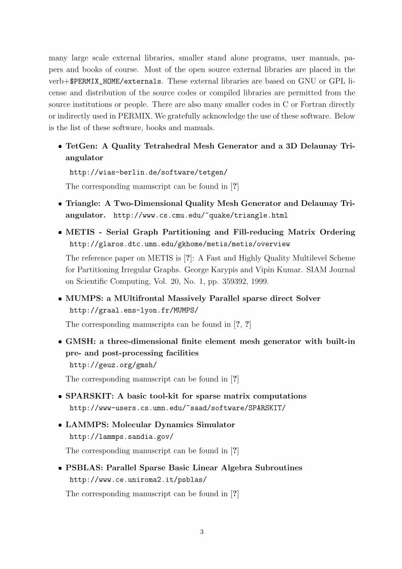
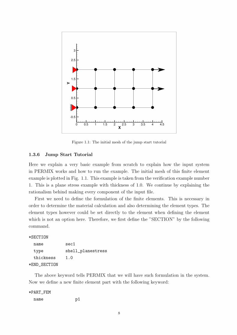
Figure 1.1: The initial mesh of the jump start tutorial

1.3.6 Jump Start Tutorial

Here we explain a very basic example from scratch to explain how the input system

in PERMIX works and how to run the example. The initial mesh of this finite element

example is plotted in Fig. 1.1. This example is taken from the verification example number

1. This is a plane stress example with thickness of 1.0. We continue by explaining the

rationalism behind making every component of the input file.

First we need to define the formulation of the finite elements. This is necessary in

order to determine the material calculation and also determining the element types. The

element types however could be set directly to the element when defining the element

which is not an option here. Therefore, we first define the ”SECTION” by the following

command.

*SECTION

name sec1

type shell_planestress

thickness 1.0

*END_SECTION

The above keyword tells PERMIX that we will have such formulation in the system.

Now we define a new finite element part with the following keyword:

*PART_FEM

name p1

8

section sec1

*END_PART_FEM

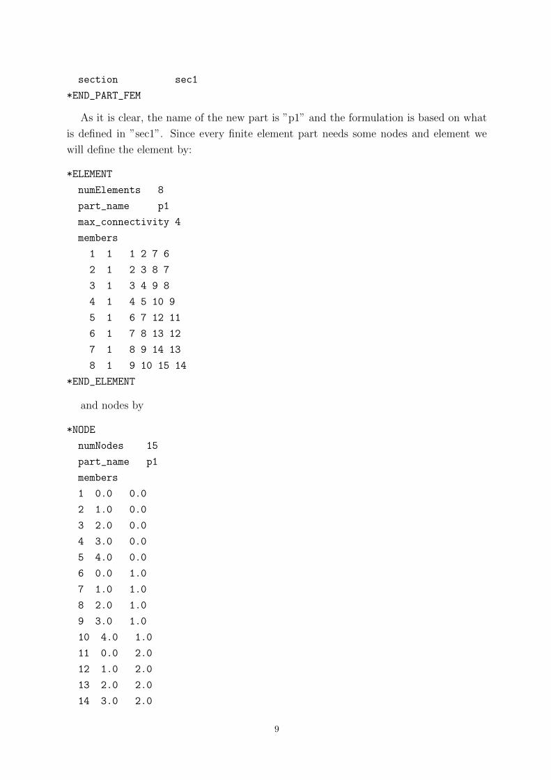
As it is clear, the name of the new part is ”p1” and the formulation is based on what

is defined in ”sec1”. Since every finite element part needs some nodes and element we

will define the element by:

*ELEMENT

numElements 8

part_name p1

max_connectivity 4

members

1 1 1 2 7 6

2 1 2 3 8 7

3 1 3 4 9 8

4 1 4 5 10 9

5 1 6 7 12 11

6 1 7 8 13 12

7 1 8 9 14 13

8 1 9 10 15 14

*END_ELEMENT

and nodes by

*NODE

numNodes 15

part_name p1

members

1 0.0 0.0

2 1.0 0.0

3 2.0 0.0

4 3.0 0.0

5 4.0 0.0

6 0.0 1.0

7 1.0 1.0

8 2.0 1.0

9 3.0 1.0

10 4.0 1.0

11 0.0 2.0

12 1.0 2.0

13 2.0 2.0

14 3.0 2.0

9

15 4.0 2.0

*END_NODE

We could define the nodes and element in a separate file in case of many number

of elements and nodes. As it can be seen from the element description, we assign the

elements to the defined finite element part, ”p1”. Also, here we have not defined the

element type. In this case PERMIX will decide for the element based on the section type

and number nodes. The element type, material number etc. can be later on changed with

the ”ELEMENT MODIFY” command.

To define the material properties, we use something like the following keyword. Every

material model should have a name and a unique ”matid”. In the element description,

the ”matid” is given.

*MATERIAL

name mat01

matid 1

type linearelastic

props 26.0 0.3

*END_MATERIAL

We will continue by defining some loading and boundary conditions. Before doing this,

we need to define some sets.

*SET

part_name p1

name set1

type nset

members

1 6 11

*END_SET

*SET

part_name p1

name set2

type nset

members

1

*END_SET

Here we have defined two sets and we would like to fix the nodes as clear from the figure.

The boundary conditions are defined by fixes and in case of fixed boundary condition, it

is defined by ”spc” style of fixes.

10

*FIX

style spc

name fxset1

set_name set1

dof 1

*END_FIX

*FIX

style spc

name fxs22

set_name set2

dof 2

*END_FIX

After defining some more boundary conditions and loading, we would like to define a

disk output since PERMIX will not output anything by default.

*DUMP

name dump1

filename linearelastic2d.plt

format tecplot

*END_DUMP

The above keyword will define a disk output (in PERMIX it is called dump) with the

Tecplot format. One can define as many output as necessary with repeating the dump

keyword and changing the dump name.

11

Chapter 2

PERMIX Scripting Commands

The PERMIX input file can have two type of commands. The first type is to ask something

from PERMIX as a utility. For example, we would like to include another file into the

current input file. The second type is the PERMIX input data for the actual analysis

such as the finite element nodes and elements. The first type can be also called a sort

of scripting. The scripting commands of PERMIX are really limited. The intention

is that the complex commands are to be implemented in Fortran (easily possible) or a

proper scripting language (not yet available) when PERMIX is compiled as a library. The

PERMIX scripting commands start with a $ and they are limited to one line only.

2.1 $end permix input

When this command is written in any line of the input file, PERIX ignores the rest of the

file.

2.2 $include

$include /djhs/sdjh/anyfile.lkj

This command will include the file /djhs/sdjh/anyfile.lkj at the place of occur-

rence. The file will NOT physically copied anywhere. It is just treated as another input

file. Therefore, this command inside the PERMIX Keywords will not work. The include

commands can be also used in an included file and PERMIX will read all in proper order.

Please refer to VERIF2 for an example.

12

Chapter 3

Keywords

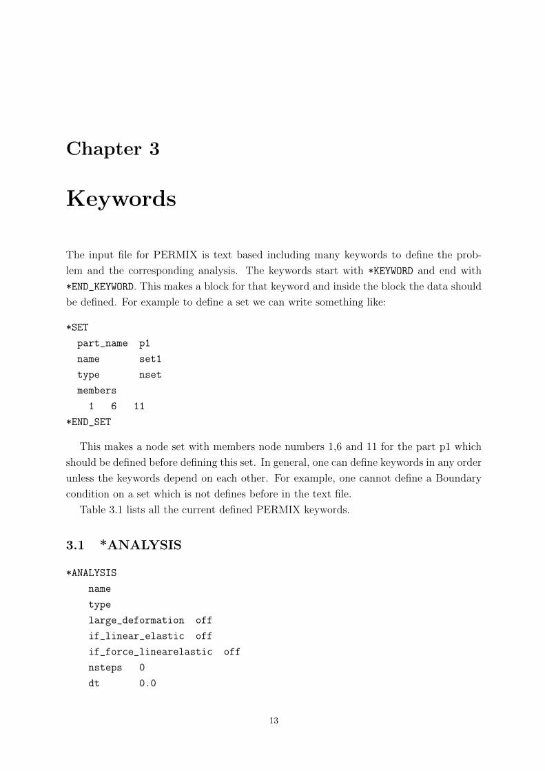
The input file for PERMIX is text based including many keywords to define the prob-

lem and the corresponding analysis. The keywords start with *KEYWORD and end with

*END_KEYWORD. This makes a block for that keyword and inside the block the data should

be defined. For example to define a set we can write something like:

*SET

part_name p1

name set1

type nset

members

1 6 11

*END_SET

This makes a node set with members node numbers 1,6 and 11 for the part p1 which

should be defined before defining this set. In general, one can define keywords in any order

unless the keywords depend on each other. For example, one cannot define a Boundary

condition on a set which is not defines before in the text file.

Table 3.1 lists all the current defined PERMIX keywords.

3.1 *ANALYSIS

*ANALYSIS

name

type

large_deformation off

if_linear_elastic off

if_force_linearelastic off

nsteps 0

dt 0.0

13

Table 3.1: A list of all PERMIX keywords

ANALYSIS Defines a step of analysis like explicit dynamics or linear elastic.

*BOUNDARY The is replaced by FIX

*COMPUTE Defines a compute on the system such as homogenized stress.

*CURVE Defines a curve based on x and y values.

*ELEMENT Defines elements of a finite element part.

*ELEMENT_MODIFY Modifies the element properties of a finite element part which are

already defined.

*FIX Defines a fix such as a boundary condition or a load.

*INITIAL_CONDITION Defines an initial condition such as a pre-crack.

*INTERACTION Defines an interaction between two parts such as an Arlequin cou-

pling between two parts.

*LOAD The is replaced by *FIX

*MATERIAL Defines a material model for the system.

*NODE Defines nodes of a finite element part.

*MATRIX_CONTROL Determines types of the matrices used; For example lumped mass

or full matrix for an explicit analysis.

*PART_ATOM Defines an atomistic part (based on the Warp code).

*PART_ATOM_MODIFY Modifies and atomistic part by sending more commands.

*PART_FEM Defines a new finite element part.

*PART_LAMMPS Defines a new LAMMPS part.

*PART_LAMMPS_MODIFY Modifies an already defined LAMMPS part.

*PART_GMSH Defines a GMSH part

*PART_ABAQUS Defines an Abaqus part.

*SECTION Defines a section which sets a formulation of a finite element part.

*SET Defines a set of nodes or elements or in general a list of entities.

*SURFACE Defines a surface based on a finite element mesh.

*SOLVER Sets the linear equation solver for the current analysis.

*TOOL Defines a tool such as converting some file type to another.

*UNFIX Deletes a Fix.

*UNIVERSE Modifies the general PERMIX object such as the logfile name etc.

14

tol_f 10.0e-6

tol_u 10.0e-3

max_iter 25

units si

time_step_fac 0.9

nsteps 0

max_iter 30

run_step on

*END_ANALYSIS

Description

� name Chooses a name for this analysis.

� type Defines the type of analysis; currently the analysis types are ”linear elastic”,

”explicit dynamics” and ”nonlinear bonet”.

� run step Values can be ”on” or ”off”. When the Analysis keyword is sent to PER-

MIX, based on the analysis type, PERMIX will invoke the particular analysis driver.

This is often the case. However, sometimes the analysis driver will be run from some

other part of the code (say in a multiscale FE2 analysis). The ”off” value will stop

PERMIX from invoking the analysis driver routine.

� large deformation: Values can be ”on” or ”off” which turns on or off the large

deformation formulation.

� if linear elastic: Performs a linear elastic calculation in the nonlinear solver (New-

ton iteration will be converged in one iteration).

� if force linearelastic: Forces PERMIX to use the default linear elastic solver.

� auto timestepping: Values can be ”on” or ”off” which during the explicit dynamic

analysis, the time step can be determined by PERMIX.

� end time: Defines end time or maximum load step of an analysis.

� time step fac: Scales the time step with this value.

� nsteps: Defines the number of time steps or load steps in the analysis.

� dt: Defines the time step of the solution in case the automatic time stepping is off.

Also, in case of nonlinear bonet analysis, it will serve as the load step.

� tol f The residual force tolerance of the convergence of the nonlinear bonet analysis.

� tol u The displacement tolerance of the convergence of the nonlinear bonet analysis.

� max iter Maximum number of Newton iterations for the nonlinear bonet analysis.

15

� units Sets the units of the analysis. The possible options can be ”lj”, ”real”, ”metal”,

”si”, ”cgs” and ”electron”.

Setting the units is especially important in the multiscale analysis where all the

components of the model should work with the same unit styles. The units styles in

PERMIX are similar to that of LAMMPS.

For style si, these are the units:

mass = kilograms

distance = meters

time = seconds

energy = Joules

velocity = meters/second

force = Newtons

torque = Newton−meters

temperature = degreesK

pressure = Pascals

dynamicviscosity = Pascal ∗ secondcharge = Coulombs

dipole = Coulombs ∗meters

electricfield = volts/meter

density = kilograms/meterdim

3.2 *CURVE

*CURVE

name

values

*END_CURVE

Defines a curve which can be used for different purposes such as applying boundary

conditions. During applying the boundary conditions for example, the value can be in-

terpolated from a curve

Description

� name Give the curve a name which should be unique for every curve.

� values Below this sub-keyword, the x and y values of the curve can be listed.

16

3.3 *DUMP

*DUMP

name

nthstep 0

filename

format

custom_style

custom_style_add

*END_DUMP

Defines a disk output of all variables of parts including the finite element, atomistic

and LAMMPS parts.

Description

� name Give the dump a name which should be unique for every dump.

� nthstep Every nth number of steps PERMIX will write a disk output.

� filename The file name and path for the output file.

� format The format of the output. Currently the possible values are ”gmsh” or

”tecplot” or ”paraview”.

� custom style By default, PERMIX will write some values such as element connec-

tivities and nodes and displacements etc. If the users intends to write only some

specific variables this optional command is used. Possible values for custom style

dumping are:

” X Y Z UN1X UN1Y UN1Z ELEMENT TYPE epsXX epsYY epsZZ epsXY epsXZ

epsYZ sigXX sigYY sigZZ sigXY sigXZ sigYZ P Damage Alpha ReactX ReactY Re-

actZ pe/atom stress/atom centro/atom ELEMENT STATUS ELEMENT MATID

Proc ORIGID ”.

The default written values are:” X Y Z UN1X UN1Y UN1Z ELEMENT TYPE

epsXX epsYY epsZZ epsXY epsXZ epsYZ sigXX sigYY sigZZ sigXY sigXZ sigYZ P

”.

� custom style add Unlike the custom style command, this command adds the vari-

ables to the default style. So all the variables declared here will be written to the

disk, along with the default variables.

17

3.4 *FIX

Fixes are methods of defining boundary conditions or loading or some other opera-

tions which need to have access over all the variables of the parts. Every fix must

have a name and a style. Currently the styles are ”spc”, ”Cload”, ”Dload”, ”Dsload”,

”crack propagation”, ”prescribedbc” and ”velocity set”.

3.4.1 Cload

Defines concentrated loads on the finite element parts which are applied directly to the

nodes.

*FIX

name

style Cload

set_name

dof

value

*END_FIX

Description

� part fem name The name of the finite element part that this fix applies.

� set name The node set which the force applies to.

� dof The degree of freedom the the force applies to.

� value The values of the force.

3.4.2 Dsload

Applied a distributed load (traction, pressure) to a surface defined by the SURFACE

command.

*FIX

name

style Dsload

surface_name

dof

value

traction

*END_FIX

Description

18

� surface name The finite element surface name which the distributed load applies

to.

� value The value of the pressure.

� traction The values of the traction load. In case traction and pressure load are both

active, then the it will give an error.

� Follower Values can be ”off” or ”on”. In large deformation the distributed loads

can rotate with the deformation.

3.4.3 Dload

Applies a body load to the finite element set such as a gravity load.

*FIX

name

style Dload

set_name

dof

value

*END_FIX

Description

� part name The name of the finite element part that this fix applies.

� set name The finite element set that the body load applies to.

� value The vector of values in x, y and z direction to aply the body load.

3.4.4 spc

Defines a fixed boundary conditions on a set of nodes of a finite element part.

*FIX

name

style spc

set_name

dof

*END_FIX

Description


� set name The node set which the boundary condition applies to.

� dof The degree of freedom the the boundary condition applies to.

19

3.4.5 prescribedbc

Applies prescribed displacements on set of nodes of a finite element part.

*FIX

name

style prescribedbc

set_name

dof

value

*END_FIX

Description


� set name The node set which the boundary condition applies to.

� dof The degree of freedom the the boundary condition applies to.

� value The prescibed value of the node set.

3.4.6 velocity set

Changes the velocity of set of nodes. By default, it will set the velocity by the value given;

however when ”sum yes” added, the velocity will be added to the existing velocity.

*FIX

name

style velocity_set

set_name

dof

value

if_bc

birth_time

death_time

curve_name

*END_FIX

Description

� set name The node set which the velocity set applies to.

� dof The degree of freedom the the velocity applies to.

� value The velocity value of the node set.

20

� curve name The name of the curve which the velocity value can be interpolated.

If a curve name is defined, then the ”value” sub-keyword will be neglected.

� birth time The fix will be applied from this time. This time overrides everything

else.

� death time The fix will NOT be applied after this time. This time overrides every-

thing else.

� if bc If yes then this fix acts as a boundary condition and the forces become zero in

the DOFs where it is applied. The default value is yes.

3.4.7 crack propagation

Activates the crack propagation on a finite element part.

*FIX

name

style crack_propagation

part_fem_name

*END_FIX

Description


The crack propagation criterion is based on the first the Element stability checks

and might be the material stability check. For example, for a linear elastic material,

an element stability is subroutine is called. Then inside that subroutine, the material

stability is checked for a point in the middle of the element. The crack propagation is

currently experimental and needs more stabilization.

3.4.8 microanalysis

This fix does different types of microstructure analysis. One is to find the grains (oper-

ation find grains) which finds the grains based on the material that is assigned to every

element. This fix primarily written for the OOF2 software and it completes its outcome

by identifying the grains which can be later used to give different orientation to them.

*FIX

style microanalysis

name mymicro1

part_fem_name p1

operation find_grains

*END_FIX

21

Description


� operation The type of the operation that is expected from this fix. The operations

can be find grains as explained above.

3.5 *COMPUTE

Computes are method of computing some parameter from the model. The computes

will not change the status of the simulation and only attempt to computed the intended

property. The current defined compute styles can be ”homogen val” and ”mcouplerr”.

3.5.1 homogen val

*COMPUTE

name

style homogen_val

part_fem_name

*END_COMPUTE

Description

� part fem name The name of the finite element part that the homogenized variable

is supposed to be computed.

3.5.2 nodalhvar

*COMPUTE

name

style nodalhvar

part_fem_name

*END_COMPUTE

Description

� part fem name The name of the finite element part.

This compute, calculates the nodal value of the history variables such as stresses.

The names of values computed here are for example ”C nodalsigXX”, ”C nodalsigYY”,

”C nodalsigZZ”, ”C nodalsigXY”, ”C nodalepsXZ”, ”C nodalHuvar26” and so on. Nearly

all the history variables can be interpolated to the nodes. In order to dump these values

on disk, one needs to first define this compute and afterwards define a dump with custom

variables and put any of the mentioned variables names to write in the output file.

22

3.6 *ELEMENT

Defines element connectivities of a finite element part (part fem). The part fem should

have already been defined in the input file.

*ELEMENT

part_name

numElements

format

max_connectivity

etype

members_gmsh_tag

members

*END_ELEMENT

Description

� part name The name of the corresponding finite element part

� numElements The number of elements provided

� format The format of the element input. This tells PERMIX the meaning of num-

bers at every row of the element reader. Two formats are possible: ”lsdyna”, which

is default and ”abaqus”. In ”lsdyna” format every row of the members will be:

#element_id #material_id #nodid_1 #nodid_2 #nodid_3 ...

In ”abaqus” format, every element row is:

#element_id #nodid_1 #nodid_2 #nodid_3 ...

� max connectivity defines maximum number of nodes per element.

� etype: defines the element type. If not defined, the element type will be determined

according to the section assigned to this finite element part.

� members: From this line below the element connectivities are listed. The members

can be also read from an external text file. To do this, after ”members”, the ”txtfile”

keyword following with the path to the text file containing the element connectivities

should be provided.

� members gmsh tag: This will extract the elements from a GMSH part.

members_gmsh_tag pgmsh_name 87

will get the elements with the tag 87 from the pgmsh_name GMSH part.

23

3.7 *ELEMENT MODIFY

After the definition of the element, if the user intends to modify certain property of the

a set of elements ELEMENT MODIFY keyword can be used.

*ELEMENT_MODIFY

part_name

matid

type #can be set_etype, set_material

etype

set_name

*END_ELEMENT_MODIFY

Description


� etype: defines the element type. If not defined, the element type will be determined

according to the section assigned to this finite element part.

� type: This determines the type of modification of the element and can be ”set etype”

or ”set material” which change the element type or the material id.

� set name: Defines the name of the set for which the change of property applies.

� matid: The new material id for the set of elements.

3.8 *INITIAL CONDITION

Initial conditions are methods of defining a type of initial condition. The possible initial

conditions are ”crack enrichment”, ”extra element” and ”initial strain”.

3.8.1 crack enrichment

Defines a crack enrichment by level sets defined by element number and the local node

number. The crack enrichment is applied as XFEM enrichment to the element. This type

of enrichment will be finally replaced by applying ”extra element” which offer a better

method of implementation.

*INITIAL_CONDITION

name

style crack_enrichment

part_name

tip_enrichment

members

*END_INITIAL_CONDITION

24

� part name The name of the part that the initial condition is applied to.

� tip enrichment Can get the values of ”on” or ”off”. If on, then the tip enrichment

is activated in XFEM. This option is not active in 3D.

� members The level set values for nodes of the particular elements.

� shifted basis Can get the values of ”yes” or ”no”. If yes, then the XFEM formula-

tion will be based on the shifted basis. Refer to the corresponding paper on shifted

basis XFEM elements. The shifted basis does not work for explicit dynamics because

of the special mass lumping technique.

3.8.2 extra element

The extra element style of initial condition, defined extra properties for elements. Some

elements accept the extra properties other than their nodes, element connectivities and

material number. For example, the SXL type elements accept enrichment (level set values)

to put an XFEM crack inside the element. The extra element in this case is a more

generic version of defining enriched elements. This type of defining extra information can

be extended to other types of elements too.

*INITIAL_CONDITION

name

style extra_element

members


� part fem name The name of the finite element part that the initial condition is

applied to.

3.9 *INTERACTION

Interactions define method of interaction between two parts. The parts can be finite

elements, atomistic or LAMMPS.

3.9.1 bdm adaptive

Based on the Arlequin method (Bridging Domain Method when atomistic coupled to

finite elements) the bdm adaptive style is defined.

*INITIAL_CONDITION

name

style bdm_adaptive

active_atom_region

25

adap_check_nthstep

adaptive_refine_size

adap_method

part_fem

part_fem_fine

part_atom

part_lammps


Description

� part fem The name of the finite element part for the coarse scale

� active atom region The region of the coarse scale which should be modelled by

the fine scale.

� part fem fine The name of the finite element part for the fine scale

� part atom The name of the atomistic part for the fine atomistic scale

� part lammps The name of the LAMMPS part for the fine atomistic scale

� adap method The adaptivity method, if not set, the adaptivity method is not

checked.

� adap check nthstep Every nth step the model is checked if the adaptivity criterion

is fulfilled.

� adaptive refine size the size of the coarse scale region which is converted to fine

scale calculation.

3.10 *MATERIAL

This keyword is used to define different material models assigned often to finite ele-

ment parts. Currently the defined material models are ”linearelastic”, ”hyperelastic pd”,

”lemaitre damage” , ”neo Hookean incomp” ,”cohesive”, ”mfesq” and ”CB LAMMPS”.

3.10.1 linearelastic

Defines a linear elastic constitutive material model.

*MATERIAL

name

style linearelastic

props

*END_MATERIAL

26

Description

� props The properties of the linear elastic material. the first parameter is the Young’s

Modulus, the socond is the Poisons ratio, third is the density of forth is the maximum

principle stress at failure.

3.10.2 hyperelastic pd

This is a hyperelastic material law in principle directions.

*MATERIAL

name

style hyperelastic_pd

props

*END_MATERIAL

Description

� props

3.10.3 lemaitre damage

This is the Lemaitre damage model which is suitable mostly for concretes. The quasi-

brittle crack propagations can be also modelled in concrete using this material.

*MATERIAL

name

style lemaitre_damage

props

*END_MATERIAL

Description The values after the ”props” keywords have the following meaning:

� Young’s Modulus

� Poisson’s ration

� density

� A

� B

� Initial strain at onset of damage

The stability check of this material model is based on the loss of ellipticity.

27

3.10.4 neo Hookean incomp

This is a hyperelastic material model and it is incompressible.

*MATERIAL

name

style neo_Hookean_incomp

props

*END_MATERIAL

Description The props values are:

� density

� shear modulus

� kappa

3.10.5 cohesive

This material defines the cohesive behaviour of a crack. It is basically used to compute

the cohesive crack forces with respect to crack opening.

*MATERIAL

name

style cohesive

max_delta

max_stress

*END_MATERIAL

3.10.6 mfesq

This material model is a multiscale material. When defined, at every point a rectangu-

lar RVE (representative volume element) full finite element system is defined and first

order homogenization method is used to compute the average strain and stiffness at the

integration points.

*MATERIAL

name

style mfesq

RVE_file

set_boundary

setp_up

set_down

set_left

28

set_right

*END_MATERIAL

Description

� RVE file: The path to the full model of the RVE file. The RVE finite must contain

a node set of all boundary nodes.

� set boundary: The string name of the set which contains the boundary nodes

� setp up: For the basic homogenization technique without periodic boundary condi-

tions, the above keywords are enough. The setp up and other similar keywords are

used to give the names of the nodes sets of the RVE at every edge of the rectangular

RVE.

3.10.7 CB LAMMPS

This material model is used to replicate the material law with the Cauchy–Born assump-

tion. The Cauchy–Born assumption homogenizes the material properties from atomistic

lattice. This case, at every integration point, we will have a full atomistic lattice with the

properties given by the ” str command”.

*MATERIAL

name mat01

matid 1

style CB_LAMMPS

str_command # 2d LJ crack simulation

str_command log log.lammps_mat_CB

str_command dimension 2

str_command boundary s s p

str_command units lj

*END_MATERIAL

Description

� str command Sends a command to the atomistic model generated by LAMMPS.

These commands must define a lattice and create the atoms. Also, atomistic poten-

tial, units, etc.

In order to use this material model, the LAMMPS packages must have been attached

to PERMIX. The Cauchy-Born method implemented in PERMIX is not temperature

dependant. In general, this method has many restrictions and careful checking of the

input parameters is needed.

29

3.11 *NODE

Defines the nodal coordinates of a finite element part (part fem). The part fem should

have already been defined in the input file.

*NODE

part_name

numNodes

members_gmsh_tag

members

*END_NODE

Description


� numNodes The number of nodes provided

� members: From this line below the nodes are listed. The members can be also

read from an external text file. To do this, after ”members”, the ”txtfile” keyword

following with the path to the text file containing the nodal coordinates should be

provided.

The style of one row of the Nodes should be like this:

#node_id #X_coordinate #Y_coordinate #Z_coordinate

� members gmsh: This will extract the nodes from a GMSH part.

members_gmsh pgmsh_name

will get the nodes from the pgmsh_name GMSH part.

3.11.1 NODAL FIELD

Defines a nodal field in two ways. 1) By element number and its corresponding node id

or simply by node ids. In the former case, the values will be unified so every node has a

unique value. In the second case, one of the values of element or local nodes should be

zero.

The example of nodal field values can be level sets, temperature and so forth.

*NODAL_FIELD

name

members

*END_NODAL_FIELD

� members The nodal field values for nodes of the particular elements.

30

3.12 *PART ABAQUS

Defines a new Abaqus part.

*PART_ABAQUS

name abaqustest

permix_output Job-1.prx

inp_file ../examples/abaqus-interface/Job-1.inp

*END_PART_ABAQUS

Description

� name Chooses a name for this part

� permix output A file name output in case a PERMIX input file is needed to gen-

erate from the Abaqus input

� use part abaqus given a part abaqus name, PERMIX will convert the abaqus input

to PERMIX part fem.

Currently, this command is useful to convert an Abaqus input file to PERMIX input

file or directly create a part fem is PERMIX from and Abaqus INP file.

3.13 *PART FEM

Defines a new finite element part.

*PART_FEM

name

section

use_part_abaqus

*END_PART_FEM

Description


� section Chooses a section for this part. The section should have already been

defined.

� use part abaqus given a part abaqus name, PERMIX will convert the abaqus input

to PERMIX part fem.

� abaqus part instance: In Abaqus INP files, there can be many instances. Every

Abaqus Instance in PERMIX can be considered as a Finite Element part. Therefore,

when a new finite element part in PERMIX is made from Abaqus, the corresponding

Abaqus instance name must be provided.

31

3.14 *PART ANSYS

Defines an ANSYS part, which is currently bunch of utility routines to convert files.

*PART_ANSYS

name

permix_output

ansys_cdb

write_elements_in_Abaqus

write_nodes_in_Abaqus

write_nodes_in_ANSYS_CDB

write_elements_in_ANSYS_CDB

*END_PART_ANSYS

Description


� ansys cdb Inputs the ANSYS cdb file, given the file name.

� write nodes in ANSYS CDBWrites nodes in the ANSYS nblock format given a

file name.

� write elements in ANSYS CDB Writes the elements in the ANSYS eblock for-

mat.

� write nodes in Abaqus Writes nodes in the Abaqus format given a file name.

� write elements in Abaqus Writes elements in the Abaqus format given a file

name.

3.15 *SET

*SET

name

type

part_name

members

members_generate

members_gmsh_tag

*END_SET

Description

� name: the name of the set

32

� type: the type of the set can be eset or nset for element and node set respectively.

� part name: the name of the part that this set belong to.

� members: on the next line, the members are listed.

� members generate: This will generate the members if there can be an implied

loop. For example

members_generate 3,10,2

will generate 3,5,7,9 as the members of the set.

� members gmsh tag: This will extract the members from a GMSH part.

members_gmsh_tag pgmsh_name 87

will get the nodes with the tag 87 from the pgmsh_name GMSH part.

� members: on the next line, the members are listed. For every member, there is

a line with two numbers. First number corresponds to the element id, and second

corresponds to the local surface id of that element.

When a set name is not given, a part name should be given so the surface can be

related to a finite element part.

3.16 *SURFACE

*SURFACE

set_name

type

surfaceid

part_name

name

members

Description

� name: the name of the surface

� set name: the element set which contains the list of the element where one of their

surfaces is selected.

� surfaceid The ID of the surface of the element.

33

3.17 *SECTION

The se

*SECTION

name

thickness

type

*END_SECTION

Description

� name: The name of the section

� thickness: In case of planestress or shell formulation, defines the thickness of the

elements.

� type: The type of the section. This type will help PERMIX to determine the element

type and compute the material properties. The section types are defined below.

The section type can be:

� shell planestrain: The plane strain shell element (can be 3 node triangular or 4

node quadrilateral with full integration.

� shell planestress: The plane stress shell element (can be 3 node triangular or 4

node quadrilateral with full integration.

� shell planestrain fast: Same implementation of the plane strain element with

faster implementation.

� shell planestress fast

� shell planestrain fast omp The OpenMP parallel version of the plane strain fast

element.

� shell planestress fast omp

� solid: Solid 8 node hex or 4 node tetrahedral element with full integration.

� solid fast A faster implementation of the solid element.

� solid fast omp

� solid omp

� shell planestrain omp

� shell planestress omp

Often, the section type plus the number of nodes of an element dictate the element

type and how the material constitutive law is computed.

34

3.18 *SOLVER

Chooses the solver and its corresponding parameters for the current solution of system

of equations. The styles that the solver can take are ”MUMPS”, ”PSBLAS3”, ”MKL”,

”MKL iter”, ”BASIC” and ”SPARSKIT”.

3.18.1 BASIC

Chooses the BASIC solver implemented in PERMIX to solve the system of equations.

This is a very basic direct sparse solver to solve very small system of linear equations.

When no other solver is attached to PERMIX, this solver is used. Please note using this

solver is not recommended. However, basic verification examples can be passed with this

solver.

*SOLVER

type BASIC

memory_const

*END_SOLVER

Description

� memory const This parameter is used to increase the internal memory for this

solver.

3.18.2 MUMPS

Chooses the MUMPS solver http://graal.ens-lyon.fr/MUMPS/ which is a parallel

direct sparse solver.

*SOLVER

type MUMPS

*END_SOLVER

3.18.3 MKL

When available, this option uses the Intel MKL direct solver to solve the system of

equations. The intel MKL is parallel for shared memory systems. Therefore in the

multicore systems, the CPU can be used efficiently.

*SOLVER

type MKL

*END_SOLVER

35

3.18.4 MKL iter

When available, this option uses the Intel MKL iterative solver to solve the system of

equations. The Intel MKL is parallel for shared memory systems. Therefore in the

multicore systems, the CPU can be used efficiently. The iterative MKL solver is useful

when a big model is running on a shared memory system.

*SOLVER

type MKL_iter

*END_SOLVER

Description

3.19 *UNCOMPUTE

Deletes a defined compute.

*UNCOMPUTE

name

*END_UNCOMPUTE

Description

� name The name of the compute to delete.

3.20 *UNFIX

Deletes a defined fix.

*UNFIX

name

*END_FIX

Description

� name The name of the fix to delete.

3.21 *UNDUMP

Deletes a defined dump.

*UNDUMP

name

*END_UNDUMP

Description

� name The name of the dump to delete.

36

Chapter 4

Developers Guide

PERMIX has a simple but effective object oriented style which utilizes the very capabil-

ities of the modern Fortran language for rapid and doable development of the numerical

methods. We begin by demonstrating the addition of most common classes and via these

examples more details of the program will be shown. In the documentation folder, we

provide these examples. The developer has to follow the description of these examples to

add a new capability to PERMIX.

4.1 Adding a Compute

Here we will show step by step addition of a new compute style. Also, we will show how

to access different data on the finite element parts. In order to understand this section,

one needs to follow the example Fortran file in:

/PERMIXHOME/documentation/usermanual/developer/compute/compute testc class.f90

Suppose we would like to add a new compute style names testc. Therefore the naming

convention of PERMIX recommends us to choose:

� testc : as the style name of our new compute

� compute_testc_class : as the Fortran module for the new compute class

� ty_compute_testc : as the new compute class name

In order to define a new compute, the newly defined derived data type (like a class in

C++) should inherit its properties from the base class of the the compute. The name of

the compute base class is ty_compute_base. Therefore, we will do the following steps:

� Add the new Fortran file (compute_testc_class.f90). As one can realize, the name

of the Fortran file is the same as the Fortran module name. Although this is not

necessary, it will ease the dependency analysis of the Fortran modules and it will

remove some confusions.

� Inside the new file, generate the Fortran module compute_testc_class

37

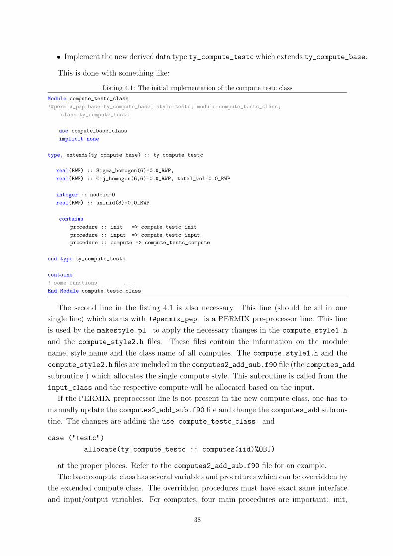
� Implement the new derived data type ty_compute_testc which extends ty_compute_base.

This is done with something like:

Listing 4.1: The initial implementation of the compute testc class

Module compute_testc_class

!#permix_pep base=ty_compute_base; style=testc; module=compute_testc_class;

class=ty_compute_testc

use compute_base_class

implicit none

type, extends(ty_compute_base) :: ty_compute_testc

real(RWP) :: Sigma_homogen(6)=0.0_RWP,

real(RWP) :: Cij_homogen(6,6)=0.0_RWP, total_vol=0.0_RWP

integer :: nodeid=0

real(RWP) :: un_nid(3)=0.0_RWP

contains

procedure :: init => compute_testc_init

procedure :: input => compute_testc_input

procedure :: compute => compute_testc_compute

end type ty_compute_testc

contains

! some functions ....

End Module compute_testc_class

The second line in the listing 4.1 is also necessary. This line (should be all in one

single line) which starts with !#permix_pep is a PERMIX pre-processor line. This line

is used by the makestyle.pl to apply the necessary changes in the compute_style1.h

and the compute_style2.h files. These files contain the information on the module

name, style name and the class name of all computes. The compute_style1.h and the

compute_style2.h files are included in the computes2_add_sub.f90 file (the computes_add

subroutine ) which allocates the single compute style. This subroutine is called from the

input_class and the respective compute will be allocated based on the input.

If the PERMIX preprocessor line is not present in the new compute class, one has to

manually update the computes2_add_sub.f90 file and change the computes_add subrou-

tine. The changes are adding the use compute_testc_class and

case ("testc")

allocate(ty_compute_testc :: computes(iid)%OBJ)

at the proper places. Refer to the computes2_add_sub.f90 file for an example.

The base compute class has several variables and procedures which can be overridden by

the extended compute class. The overridden procedures must have exact same interface

and input/output variables. For computes, four main procedures are important: init,

38

input, setup and compute. The init and input procedures are called directly after the

object allocation at the input time. After calling init, the input procedure will be called

and the input keyword is passed to this subroutine. All of these are done automatically.

We clarify with an example. Please refer to the linearelastic.prx file in the compute

documentation folder. This file is the same example as presented in the jump start section

with an additional compute keyword.

After the definition of the finite element part, ”p1” in the input file, now would like to

for example, show the element connectivities of the ”p1” on the screen using our newly

developed compute. Thus, we add this keyword to the input file:

*COMPUTE

name myfirstcompute

style testc

part_fem_name p1

*END_COMPUTE

When the input_class reaches this keyword, it will call the computes_add subroutine.

This subroutine will allocate polymorphic compute variable with a ty_compute_testc

style and calls compute_testc_init subroutine. One can do all the initialization in the

init subroutine. Next, computes_add subroutine will call the compute_testc_input sub-

routine and passes the keywords (from *COMPUTE to *END_COMPUTE) to compute_testc_input

subroutine. In this subroutine the keywords are being analysed. For example, we can de-

fine a new sub-keyword in the compute_testc class to read the name of a finite element

part and based on the name, associate the pointer part_fem to this finite element part.

The setup procedure will be called before the actual analysis starts. If a procedure

is not overridden in the extended derived data type, the original procedure from the

base class will be executed. In our case, we did not define the setup procedure there-

fore the computes_setup from the compute base class will be called. The execution

of the ”compute” procedure is usually done at the end of the step when an output is

requested. In our linear elastic example, the compute_testc_compute subroutine will

be called after the solution of the equations. Please refer to extensive comments in the

compute_testc_class.f90 file for various usage of PERMIX data structure.

4.2 Adding a Step

Steps classes are used to perform a single analysis step on the parts. For example, a

step can be a linear elastic or explicit dynamic analysis. The steps are relatively easy to

implement and they have access to all parts, computes and fixes. The analysis_class

will determine the properties of the steps. For example, what is the load increment for a

nonlinear static solution or the end time for the explicit dynamic step.

39

The step_base_class is the base class for defining the step. Similar to computes, the

derived data types of new steps should inherit the properties of the base step class. To

give an example, we have provided and example in the test_step_class.f90 file which

is both in the source codes and documentation.

In order to add the new test_step_class we created the new file with lines below

(refer to the source code in PERMIX sources or the source code in manual for the complete

working file).

Listing 4.2: The initial implementation of test step class

Module test_step_class

use step_base_class

implicit none

type,extends(ty_step_base) :: ty_test_step

contains

procedure :: execute => test_step_execute

procedure :: setup => test_step_setup

end type ty_test_step

contains

! some functions ....

End Module test_step_class

After adding the new step class, the step allocation routine must be changed similar

to the compute allocation. This is done in the step_add.f90 file and the step_add2

subroutine. As in listing 4.3, two places must be modified to add the new step.

Listing 4.3: Modifications to add a new step class

use test_step_class ,gugu6=>step_add2

...

case ("test_step"); allocate(ty_linear_elastic :: step)

After modification of the step_add2 subroutine, no more change is necessary and the

step will be called automatically when invoking this in the input:

*ANALYSIS

type test_step

name test_new_step

*END_ANALYSIS

Every step has two important procedures 1)setup 2) execute. The setup procedure will

do some preliminary tasks such as allocation of matrices, initial setup of computes and

fixes an so on. In the execution phase the problem will be solved. The newly test step

class implement a linear elastic step and every line is explained in detail.

40

Remark 1: The step classes are created at the time of run and destroyed after they

finish.

Remark 2: Although the step classes have access to all parts, one can implement a

new step class which acts on one part only with some assumptions. However, the current

implemented analysis steps acting on all relevant parts while this is not necessary for

general.

Remark 3: In the setup phase of the steps, two important issues must be addressed:

1) which vectors and matrices must be allocated 2) what matrices and vectors should

be computed at the element level. For example, for a linear elastic analysis we need to

allocate the stiffness matrix, external force vector and displacement vector. We also need

to tell the element calculator to compute the initial stiffness. The external forces will be

computed in the fixes and the solution is done in the step class where it calls the PERMIX

solver.

4.3 Adding an Element

4.3.1 General Comments

Adding a new finite element can be the trickiest task in PERMIX. This is because elements

are dependant on several other classes such as section_class and analysis_class and

others. Elements in PERMIX also have a base class similar to computes. In the ele-

ment base class FEM_element_base_class all the element types are defined as constant

numbers (enum in Fortran). Therefore every element type has a unique number assigned

to it. Also, the elements types can be recognized according to their section type. For

example if we define a part fem with section type ”solid”, and we define no element type

during element definition (the *Element keyword ), PERMIX will automatically assign

the element type to ”FEM V8N” element type for eight node elements or ”FEM V4N”

for four node tetrahedral elements.

As a result, one often needs to define the section types and number of nodes which

corresponds to a certain element type. The section type is also important to compute

the material properties. The definition of the element type constants and section type

correspondence to the element types is in the FEM_element_base_class.f90 file. In the

same file the abstract data types for elements can be seen.

Another point is the ability of the element to compute different properties. For ex-

ample, one element can compute the mass matrix and the other cannot. Or an element

can compute traction loads while the other one is not able to. This is called the ele-

ment capability in PERMIX and in the element base class, the logical variables such as

if_f_internal and if_boundary_pressure tell the user of the element if the element

41

is able to compute the internal forces or boundary pressure receptively. For full list of

element capability definition refer to the source code of the base element class.

Image we would like to do a linear elastic analysis as in the file linear_elastic_class.f90

is doing the task in two steps 1) setup of the analysis 2) execution of the step. In the

setup step, the command

analysis%needed_matrices%inital_stiffness=.true.

will ask all the elements defined for this solution to compute the initial stiffness of the

system. The needed_matrices subclass defines what matrices and vectors are needed to

be computed at the element level. At the element level these needed matrices are cross

checked versus the element capabilities and an error is sent to output in case the element

cannot compute what is needed.

Before any computation (stiffness matrix computation) at the element level, the ele-

ment type must run the element%setup routine to initialize many variables in the element.

For example, the element%nnode which tells the number of nodes for this element will

be set to 4 for a four node quadilateral element. There can be many tasks to do in the

element setup phase which depends on the implementation of the element. For example,

we can allocate some variables needed to compute the stiffness such as the B matrix and

so on.

The element%setup is a full setup which often depends on the input that means some of

the variables cannot be clear until the user defines the element, the section type for exam-

ple. However, many variables can be defined by default such as number of nodes or num-

ber of gauss points per element. Therefore, PERMIX defines a element%setup_minimal

routine which defines these initial data.

4.3.2 element index class

For efficiency reasons, to compute different matrices and vectors on the element level,

PERMIX computes the properties with one element type at a time. For example, when

the our mesh comprises of both triangular and quadilateral meshes, PERMIX indexes all

the triangular elements into a list and the element calculation is done for this list. Then

it moves to the next element type. The element_index_class is a class which takes care

the element indexing according to the element type.

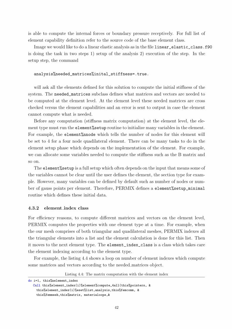
For example, the listing 4.4 shows a loop on number of element indexes which compute

some matrices and vectors according to the needed matrices object.

Listing 4.4: The matrix computation with the element index

do i=1, this%nelement_index

Call this%element_index(i)%element%compute_4all(this%pointers, &

this%element_index(i)%eset%list,analysis,this%femcomm, &

this%femmesh,this%matrix, materialoops,&

42

this%hisvars,err_code,error_message)

enddo

In the listing 4.4, this refers to a part fem object. We have then this%nelement_index

number of element types defined in this part fem and the list of the elements with one

type is stored in the this%element_index(i)%eset%list as a vector of integer numbers.

To compute different loadings and fixes same strategy can be exploited to compute the

properties. Therefore, the fixes also can have an element index object separately.

In the element_index2_class.f90 file, there is also a separate variable defined which

contains all the element defined in PERMIX and all the elements have done the basic

setup procedure of the elements. This variable is called all_elements and is accessible

in most of the PERMIX classes. For example to get the number of dimensions for the

element type FEM A4N we can simply write

Listing 4.5: Access to number of dimension of an element

ndime=all_elements(FEM_A4N)%OBJ%ndime

This provides a generic way to access to element properties. Although, this is slow and

prevent vectorization, it might be useful in many situations.

4.3.3 Procedures for Element types

When called from the step classes, every element has two important procedures: ”com-

pute 4all: and ”compute 4one”. The ”compute 4all” procedure will get the finite element

mesh and compute the need matrices and saves the results in the matrix object of every

finite element part. Teh ”compute 4all” procedure, will call the ”compute 4one” routine

which computes the values for one element and sends per element data back to the ”com-

pute 4all”. Then ”compute 4all” will assemble the local vectors and matrices into global

ones.

43

PERMIX A Platform for Multiscale...

Documents

Transcript of PERMIX A Platform for Multiscale...