Biogeosciences Discuss., 3, 1809–1858, 2006www.biogeosciences-discuss.net/3/1809/2006/© Author(s) 2006. This work is licensedunder a Creative Commons License.

BiogeosciencesDiscussions

Biogeosciences Discussions is the access reviewed discussion forum of Biogeosciences

Quantifying biologically and physicallyinduced flow and tracer dynamics inpermeable sedimentsF. J. R. Meysman1, O. S. Galaktionov1, P. L. M. Cook2,*, F. Janssen2, M. Huettel3,and J. J. Middelburg1

1Centre for Estuarine and Marine Ecology (CEME), The Netherlands Institute of Ecology(NIOO-KNAW), Korringaweg 7, 4401 NT Yerseke, The Netherlands2Max Planck Institute for Marine Microbiology, Celsiusstr. 1, Bremen, 28359, Germany3Department of Oceanography, Florida State University, Tallahassee, FL 32306-4320, USA*now at: CSIRO Land and Water, 120 Meiers Rd Indooroopilly, 4075, Qld, Australia

Received: 20 November 2006 – Accepted: 24 November 2006 – Published: 8 December 2006

Correspondence to: F. J. R. Meysman (f.meysman@ nioo.knaw.nl)

1809

Abstract

Insight in the biogeochemistry and ecology of sandy sediments crucially depends ona quantitative description of pore water flow and the associated transport of varioussolutes and particles. Here, we compare and analyse existing models of tracer dynam-ics in permeable sediments. We show that all models can be derived from a generic5

backbone, consisting of the same flow and tracer equations. The principal differencebetween model applications concerns the geometry of the sediment-water interfaceand the pressure conditions that are specified along this boundary. We illustrate thiscommonality with four different case studies. These include biologically and physicallyinduced pore water flows, as well as simplified laboratory set-ups versus more com-10

plex field-like conditions: [1] lugworm bio-irrigation in laboratory set-up, [2] interactionof bio-irrigation and groundwater seepage on a tidal flat, [3] pore water flow inducedby rotational stirring in benthic chambers, and [4] pore water flow induced by unidi-rectional flow over a ripple sequence. To illustrate the potential of the generic modelapproach, the same two example simulations are performed in all four cases: (a) the15

time-dependent spreading of an inert tracer in the pore water, and (b) the computationof the steady-state distribution of oxygen in the sediment. Overall, our model compar-ison indicates that model development is promising, but within an early stage. Clearchallenges remain in terms of model development, model validation, and model imple-mentation.20

1 Introduction

Sandy sediments make up a substantial part of coastal and shelf areas worldwide, andconsequently, they form an important interface between the aquatic environment andthe earth surface (Huettel and Webster, 2001). A prominent characteristic of sandysediments is their high permeability, which allows pressure gradients to force a flow25

through the pore spaces. This pore water flow forms an effective transport mechanism

1810

for various abiotic components, like solutes (Webb and Theodor, 1968) and fine clayparticles (Huettel et al., 1996), but also acts as a vector for biological particles, suchas bacteria and algae (Rush and Huettel, 2000). Previous studies have shown thatadvective transport exerts a major control on sediment biogeochemistry (e.g. Forsteret al., 1996; Shum and Sundby, 1996), microbial ecology (e.g. de Beer et al., 2005),5

and solute exchange across the sediment-water interface (e.g. Huettel et al., 1998).Therefore, our understanding of the biogeochemistry and ecology of sandy sedimentscrucially depends on a quantitative description of pore water flow and the associatedtransport of various solutes and particles.

The pressure gradients that drive pore water flow in sandy sediments are gener-10

ated by physical and biological factors. Physically driven pore water flow may resultfrom wave action leading to oscillatory pressure fields and currents (Riedl et al., 1972;Precht and Huettel, 2003) or from unidirectional bottom currents interacting with thetopography of the sediment-water interface (Thibodeaux and Boyle, 1987). This bot-tom topography may have a pure physical origin, such as sand ripples induced by15

currents, or can be created by biology, such as the pits and sediment mounds of vari-ous benthic organisms, like mud shrimp, lugworms and rays (Huettel and Gust, 1992b;Ziebis et al., 1996). Yet, pore water flow may also be directly induced by burrowingorganisms, a process typically referred to as bio-irrigation (Aller, 2001; Meysman etal., 2006a). To sustain an aerobic metabolism, benthic fauna flush their burrow struc-20

tures with oxygen-rich water from the overlying water column (Gust and Harrison, 1981;Webb and Eyre, 2004). In sandy sediments, water may be actively pumped across theburrow wall, thus generating pore water flows in the sediment surrounding the burrow(Foster-Smith, 1978; Meysman et al., 2005). Such advective bio-irrigation significantlyalters the flux, consumption and distribution of various solutes within the pore water25

(Timmermann et al., 2002; Meysman et al., 2006a, b).In order to interpret field data and biogeochemical process rates, the flow pattern

within the sediment needs to be well constrained, regardless of whether it is inducedby a physical or biological mechanism. Unfortunately, the in situ characterization of

1811

advective transport in sandy sediments is challenging for a number of reasons. Firstly,the flow pattern is three-dimensional, while pore pressure and tracer concentrationsare typically assessed by point measurements. Even with novel tracer imaging tech-niques, based on arrays of point measurements, it remains very difficult to constrainthe flow pattern (Precht and Huettel, 2004; Reimers et al., 2004). A second problem5

is that tracer measurements cannot be performed without inflicting a significant distur-bance to the sediment. The insertion of electrodes, planar optodes, benthic chambersor other measuring devices into sandy sediment implies that artificial obstacles are in-troduced for the pore water flow and/or that the overlying currents are disturbed. Sucha change in boundary conditions might drastically alter the flow pattern within the sed-10

iment. Thirdly, the pressure fields that induce pore water flow in sandy sediments arevery dynamic by nature. Key physical forcings such as sediment topography, wavesand currents can vary dramatically over short time scales (Wheatcroft, 1994; Li andAmos, 1999). A similar variability also characterizes biologically-induced flow, wherebio-irrigating organisms may change their position and adapt their pumping rate over15

time scales of minutes to days (Kristensen, 2001). Obtaining representative measure-ments under all likely combinations of these forcings is virtually impossible.

Given these difficulties associated with experimental methods, mathematical model-ing could provide a valuable and complementary tool to quantify in-situ flow patternsin sandy sediments and assess their biogeochemical effects (Meysman et al., 2005).20

Models could be used to interpret tracer data obtained from experiments, to assesspotential distortions introduced by measuring devices, or to examine complex field-likeconditions that cannot be reproduced in the laboratory. A number of model studies havebeen performed to assess flow patterns in sandy sediments, including wave-inducedadvection below sand ripples (Shum, 1992), unidirectional flow over triangular ripples25

(Savant et al., 1987; Elliott and Brooks, 1997a; Bayani Cardenas and Wilson, 2006),pore water flow in stirred benthic chambers (Khalili et al., 1997; Cook et al., 2006),and irrigational flows induced by organisms (Meile et al., 2003; Meysman et al., 2005,2006a, b). These applications clearly demonstrate the potential of numerical modeling

1812

to further our understanding of advective transport in sandy sediments. Yet, on thewhole, model development is still within an early stage, and models are far from be-ing used as a routine tool in biogeochemical studies of sandy environments. In orderto achieve this, model research should address several aspects. Firstly, most modelstend to focus on the hydrodynamics, predicting pressure fields and flow patterns within5

the sediment. But it is very difficult to measure pore pressures and velocities in thenatural environment, so these hydrodynamic variables must be indirectly constrainedfrom tracer experiments. To date, only a few models have actually coupled pore waterflow models to reactive transport models that simulate tracer behavior and sedimentgeochemistry (Meysman et al., 2006a, b; Cook et al., 2006). Secondly, there is a need10

for comparison and integration of the existing model approaches. Models have beendeveloped to study specific mechanisms of advection. The associated model formula-tions differ in the software that is used, the approximations incorporated, the boundaryconditions implemented, and even in the basic model equations (e.g. Darcy versusBrinkman formulation; see discussion below). These differences make cross-system15

comparisons difficult. Therefore, it would be valuable to apply a single model approachto different mechanisms of advective flow. Thirdly, the validation of models is still withina preliminary stage. To gain confidence in a model’s performance, model results shouldbe thoroughly and extensively compared with experimental data obtained for differenttracers under a wide range of boundary conditions.20

To increase the confidence and generality of sandy sediment models has been a ma-jor focus within two recent EU-supported research projects, termed COSA (COastalSAnds as biocatalytic filters; Huettel et al., 2006) and NAME (Nitrate from Aquifersand influences on the carbon cycling in Marine Ecosystems; Postma et al., 2005). Toachieve this, a three-step procedure was envisioned. [a] Process models are devel-25

oped for a small-scale laboratory benchmark set-up, simulating the pore water flowand the resulting reactive transport. [b] In these simplified set-ups, tracer experimentsare carried out under well-controlled conditions, and performance of the process modelis validated against these data. [c] When the process model successfully reproduces

1813

the benchmark set-up, it can be subsequently extrapolated to simulate flow patternsand tracer dynamics in more complex field conditions. The implementation of this (am-bitious) scheme is in various stages of progress for different mechanisms of pore waterflow. Here, we illustrate the current state of model development, validation and appli-cation for these different situations, reviewing past work as well as providing directions5

for future research. To emphasize the commonality between approaches, we apply ageneric modeling procedure to four different types of advective transport: [1] lugwormbio-irrigation in laboratory set-up, [2] interaction of bio-irrigation and groundwater seep-age on a tidal flat, [3] pore water flows in stirred benthic chambers, and [4] pore waterflows induced by unidirectional flow over a sequence of ripples (see overview in Fig. 1).10

These case studies include both biologically and physically induced pore water flows,as well as simplified laboratory set-ups versus more complex field-like conditions.

2 Model development: a generic approach for pore water flow and reactivetransport

In all four model applications, we used the same software and we followed the same15

procedure to quantify flow patterns and tracer dynamics. This generic modeling ap-proach consists of two parts. In a first step, the pressure and velocity fields within thepore water are described by a “flow model”. In the development of this “flow model”, thekey aspects are the justification of the approximations in the momentum equation, theproper delineation of the model domain, and the selection of the appropriate boundary20

conditions at the boundaries of this model domain. In a second step, the computedvelocity field is used as an input for a reactive transport model, which describes theevolution of certain tracer concentrations in the pore water. All model development andsimulations are performed using finite element package COMSOL Multiphysics™ 3.2a.The scripts of the various models are publicly available, and can be downloaded from25

http://www.nioo.knaw.nl/ppages/ogalaktionov/. These model scripts allow the user toadjust model domain geometry, as well as sediment and tracer properties.

1814

2.1 Simplification of the momentum equation

The starting point for model development is the specification of momentum balancefor the pore water. Existing flow models however differ in the level of detail that isincorporated in such a momentum balance. Khalili et al. (1999) proposed the Darcy-Brinkman-Forchheimer (DBF) equation as the most “complete” momentum balance5

ρ[

1φ

∂v d

∂t+

1φ

(v d · ∇) v d

]= −∇p + ρg∇z + µ∇2v d − µ

kv d − ρ

Cf√k‖v d ‖ v d (1)

where k denotes the permeability, µ the dynamic viscosity of the pore water, µ theeffective viscosity, ρ the pore water density, Cf a dimensionless drag coefficient, g thegravitational acceleration, and z the vertical coordinate. The Darcy velocity v d is re-lated to the actual velocity of pore water as v d=φv , where φ is the porosity. In the10

DBF equation, the total acceleration (left hand side) balances the forces due to pres-sure, gravitation, viscous shear stress (Brinkman), linear drag (Darcy), and non-lineardrag (Forchheimer). The DBF Eq. (1) has the advantage of generality, but may alsoengender needless complexity. In this review, we exclusively focus on sands, that is,permeable sediments with a grain diameter less than 2 mm (thus excluding gravels).15

For sandy sediments, the DBF Eq. (1) can be substantially simplified. Numerical exper-iments by Khalili et al. (1997) showed that the acceleration and Forcheimer terms arenegligibly small in sands. These two terms only become important when pore veloci-ties are really high, like in highly-permeable gravel beds. Accordingly, the momentumbalance for sandy sediments readily simplifies to20

− ∇p + ρg∇z + µ∇2v d − µkv d = 0 (2)

This so-called Darcy-Brinkman equation forms the basis for the benthic chamber modelof Khalili et al. (1997, 1999). However, one issue is whether the Brinkman term is reallyneeded in the momentum equation. Khalili et al. (1999) argued that it should be in-cluded to accurately describe advective transport. The Brinkman term is however only25

1815

important in a transition layer between the overlying water and the sediment, wherethe velocity profile exhibits strong curvature (∇2

v d large). So, the question whether ornot to retain the Brinkman term crucially depends on the thickness δ of this transitionlayer. Goharzadeh et al. (2005) investigated δ-values for grain sizes from 1 to 7 mm,and found that δ roughly equals the grain size diameter. In other words, in sands with5

a median grain size less than 2 mm, the transition layer is small compared to the scaleof the advective flow induced by waves, ripples and bio-irrigation, which is on the orderof centimeters to decimeters. Accordingly, for practical modeling applications in sandysediments, the Brinkman and other non-Darcian terms can be justifiably discarded.

2.2 Flow model10

From the viewpoint of the overlying water, the neglect of the small Brinkman transitionlayer implies that the sediment is regarded as a solid body, and a no-slip boundarycondition applies at the sediment-water interface. From the viewpoint of the sediment,it implies that the momentum balance (1) simply reduces to Darcy’s law

v d = −kµ

(∇p − ρg∇z) (3)15

Equation (3) has been used in most models of sandy sediment advection (Savant etal., 1987; Brooks et al., 1997a; Meysman et al., 2005; Bayani Cardenas and Wilson,2006), and is also the starting point of all model development here. We assume thatthe pore water is incompressible and that the tracer concentration does not affect thedensity ρ. Then, introducing the effective pressure pe=p−ρgz as the excess pressure20

over the hydrostatic pressure, one can substitute Darcy’s law (3) into the continuityequation ∇ · v d=0, to finally obtain

∇ ·(−kη∇pe

)= 0 (4)

If one assumes that the sediment is homogeneous, and so the permeability, poros-ity, and pore water viscosity remain uniform over the model domain, expression (4)25

1816

reduces to the classical Laplace equation

∇2pe = 0 (5)

Appropriate boundary conditions are needed to compute the pressure distribution andthe associated pore water velocity field from Eqs. (5) and (3). These boundary condi-tions differ between individual models and are discussed below.5

2.3 Reactive transport model

Once the pore water velocity v is computed, it can be substituted in the mass conserva-tion equation for a solute tracer in the pore water (Bear and Bachmat, 1991; Boudreau,1997; Meysman et al., 2006)

∂Cs

∂t+ ∇ · (−D · ∇Cs + vCs) − R = 0 (6)10

where Cs denotes the tracer concentration, D denotes the hydrodynamic dispersiontensor and R represents the overall production rate due to chemical reactions (whereconsumption processes are accounted for as negative production). The hydrodynamicdispersion tensor can be decomposed as D=Dmol+Dmech, representing the effects ofboth molecular diffusion and mechanical dispersion (Oelkers, 1996). The part due to15

molecular diffusion is written as (Meysman et al., 2006)

Dmol = (1 − 2 lnφ)−1 DmolI (7)

where Dmol is the molecular diffusion coefficient, Iis the unit tensor, and the multiplier(1 − 2 lnφ)−1 forms the correction for tortuosity (Boudreau, 1996). The mechanicaldispersion tensor Dmech is given the classical form (Freeze and Cherry, 1979; Lichtner,20

1996)

Dmech = DT I +

1

‖v ‖2(DL − DT ) v v T (8)

1817

The quantities DT and DL are the transversal (perpendicular to the flow) and longi-tudinal (in the direction of the flow) dispersion coefficients, which are expressed as

functions of grain-scale Peclet number P e ≡ dp‖v ‖/Dmol where dp stands for the

median particle size (Oelkers, 1996).

DT = Dmol0.5 {P e}1.2 (9)5

DL = Dmol0.015 {P e}1.1 (10)

The formulas (9) and (10) are valid for Peclet numbers in the range 1÷100, whichapplies to the models presented here (this was verified a posteriori).

2.4 Implementation and numerical solution

In the simulations presented here, we assume that environmental parameters (poros-10

ity, permeability, diffusion coefficients) do not vary over the model domain, primarilyto facilitate the comparison between models. Spatial heterogeneity can be importantunder natural conditions (e.g. the permeability in a sand ripple can be markedly differ-ent from the sediment below), yet its importance for flow patterns and tracer exchangehas hardly been addressed, and hence, this is clear topic for future research. Further-15

more, we assume that changes in the tracer concentration do not significantly influ-ence the pore water properties (density, viscosity). This is a realistic assumption thatsignificantly simplifies the simulations, as the flow model becomes decoupled from thereactive transport model. Accordingly, the flow model is solved first, and subsequently,the resulting flow field is imported into the reactive transport model. The flow model20

is implemented using the “Darcy’s Law” mode in the Chemical Engineering Moduleof COMSOL Multiphysics 3.2a. The reactive transport model is implemented usingthe “Convection and Diffusion” mode of the same Chemical Engineering Module. Allmodel parameters can be adjusted in corresponding script files (M-files). These filescan be executed via the MATLAB interface of COMSOL, or they can be run using the25

1818

newly developed COMSOL Scripts™ package. The usage of scripting allows an easyadjustment of model constants and geometrical parameters.

3 Generic modeling approach: four case studies

In the previous section, we presented a generic approach to describe flow and tracerdynamics in permeable sediments. We now apply this method to four different case5

studies. Each of these four models applies the same set of model equations: theLaplace Eq. (5) for the flow and the reactive-transport Eq. (6) for the tracer dynamics.Moreover, each of the four models incorporates a similar model domain: either theisolated sediment core that is used in laboratory incubations, or some representativesediment compartment in the field. In all cases, the lower and lateral sides of the model10

domain are considered as closed. Therefore, the principal difference between the fourmodels becomes the interaction between the overlying water and the sediment: themodels will differ in the geometry of the sediment-water interface and the boundaryconditions that are specified along this interface. In the next paragraphs, we provide arationale for the development of each model, and a detailed discussion of the boundary15

conditions at the sediment-water interface.

3.1 Bio-irrigation in a laboratory incubation set-up: model [1]

Our case study of biological flow focuses on the advective bio-irrigation induced by thelugworm Arenicola marina. Lugworms are abundant in coastal sandy areas worldwide,and are dominant bio-irrigators in these systems (Riisgard and Banta, 1998). They20

inject burrow water at depth, which causes an upward percolation of pore water andseepage across the sediment-water interface (Timmermann et al., 2002; Meysman etal., 2005). Because of their strong irrigational effects, lugworms are frequently usedin studies of advective bio-irrigation (Foster-Smith, 1978; Riisgard et al., 1996). Model[1] describes the laboratory incubation set-up (Fig. 1a) that is commonly used to study25

1819

lugworm bio-irrigation. Model [1] was proposed in Meysman et al. (2006a) to analyzelugworm incubation experiments with inert tracers. In a follow-up study on model com-plexity, model [1] was compared to a range of simpler and more complex bio-irrigationmodels (Meysman et al., 2006b).

3.1.1 Problem outline5

Lugworms pump overlying water into their J-shaped burrows, which is then dischargedinto the sediment, across the walls of a so-called “injection pocket” at the end of theburrow. The burrow walls essentially form an extension of the sediment-water inter-face. So when modeling lugworm bio-irrigation, a key issue is the representation ofthe internal structure of the lugworm burrow. This problem was recently investigated in10

detail by Meysman et al. (2006b), where 3-D models of the J-shaped burrow and thesurrounding sediment were compared to simplified 2-D and 1-D versions. The basicconclusion was that to a good approximation, the actual geometry of the burrow canbe ignored when modeling the pore water flow. This is because the walls of the burroware impermeable to flow, with the exception of the injection pocket. The burrow thus15

acts as an impenetrable obstacle to the flow, and because the burrow is small, thisonly causes a small distortion of the flow pattern. So, it suffices to model the injec-tion pocket where the burrow water is actually pumped into the surrounding sediment(Meysman et al., 2006a, b). Adopting a spherical (radial-symmetric) injection pocket,one can introduce a substantial model simplification (Fig. 2a). Physically, the model20

domain remains 3-D, but mathematically, it can be described by a radial-symmetric 2-Dmodel that incorporates two variables (the depth z and the distance r from the centralsymmetry axis).

3.1.2 Model domain and boundary conditions

The sediment domain is a cylinder of radius Rs and height Hs. The injection pocket25

is represented as a spherical void of radius Rb located at the domain’s symmetry axis

1820

at depth Hb. A triangular unstructured mesh was used to discretize the model domainwith a higher resolution near the injection pocket (Fig. 2a). At the lateral sides and thebottom of the incubation core the no-flow condition is adopted. The actual sediment-water interface consists of two parts: the flat sediment surface and the surface of theinjection pocket. At the sediment surface, the excess pressure is constant and set to5

zero, which allows the pore water to leave the sediment domain. Along the surface ofthe injection pocket the lugworm’s pumping activity imposes a constant excess pres-sure pip

e . However, no data are available on pipe as this parameter is difficult to access

experimentally. Instead, the lugworm’s pumping rate Q is usually reported, which mustmatch the discharge of water across the surface of the injection pocket. When the size10

of the injection pocket is small compared to both the burrow depth Hb and the sedimentcore radius Rs, one can directly impose a uniform flux ‖v d ‖ = Q

/Aip along the injec-

tion pocket, where Aip is the surface area. When the injection pocket is small, pressurevariations along its surface will be small, and so the flow field that is generated by im-posing a uniform flux will be identical as when imposing a constant pressure pip

e . When15

the size of the injection pocket is relatively large, we implemented a two-step procedureto derive the required pf p

e value from the known pumping rate Q. First, the flow fieldis calculated for some trial value ptest

e and the associated discharge Qtestis evaluated.Then due to the linearity of Darcy’s law, the pressure pip

e corresponding to the actualflux Q is simply calculated as20

pipe = ptest

eQ

Qtest(11)

Both types of boundary conditions options (small and large injection pockets) are im-plemented as alternative options in the M-file.

1821

3.2 Interaction between bio-irrigation and upwelling groundwater in an intertidal sed-iment: model [2]

Model [2] basically implements the bio-irrigation process model [1] in a field applica-tion for a Danish beach site, where the bio-irrigation of lugworms interacts with theupwelling of fresh groundwater (Fig. 1b).5

3.2.1 Problem outline

In recent decades, there is an increased transfer of nitrate from terrestrial areas withintense agriculture to the coastal zone. This results in the eutrophication of coastalwaters, causing algal blooms and deterioration of water quality, with significant effectson biodiversity and ecosystem functioning. The default assumption is that most ni-10

trate reaches the sea via riverine input, yet an unknown quantity percolates throughthe seabed as nitrate-rich groundwater. To this end, the discharge of nitrate-bearinggroundwater into Ho Bay (Wadden Sea, Denmark) was investigated within the multi-disciplinary EU-project NAME (Postma, 2005). The tidal fluctuation in Ho Bay is about1.5 m, and ground water (nitrate ∼0.6 mM, no sulfate) percolates up through the sandy15

beach at localized sites within the intertidal area (nitrate ∼0.03 mM, sulfate 20 mM).Within the upper centimeters of the sediment, the groundwater-derived nitrate comes

into contact with fresh organic matter, originating from primary production within thebay. Because of the high nitrate concentrations, one would expect that denitrificationwould be the dominant pathway of organic matter mineralization within the surface20

sediment. Although high denitrification rates were measured, an intriguing observa-tion was that the sediment also contained high pyrite concentration, thus indicatingsulfate reduction (G. Lavik, personal communication). This would imply that two par-allel pathways of organic matter processing are active: a terrestrial (using nitrate fromground water) along a marine (using sulfate from the overlying water). Based on ther-25

modynamic free-energy constraints and bacterial physiology, denitrification and sulfatereduction are mutually exclusive, and therefore, a proper explanation was needed to

1822

reconcile the occurrence of these two parallel pathways.One hypothesis that was forwarded as a possible explanation focused on the inter-

action between lugworm bio-irrigation and the upwelling of groundwater. Lugwormsare the dominant macrofauna species in the Ho Bay intertidal area where groundwaterseepage occurred, with densities up to 25 ind. m−2. The injection of overlying seawa-5

ter by these lugworms could create marine micro-zones within an otherwise freshwaterdominated sediment (Fig. 1b). To investigate this effect, model [2] was newly developed(in contrast to model [1], model [2] has not been previously reported in literature).

3.2.2 Model domain and boundary conditions

Similar to model [1] we consider a cylindrical sediment domain (Fig. 3a). Rather than10

a laboratory core, this model domain now represents the territory of a single lugworm

on the Ho Bay field site. The domain radius can be calculated as Rs= (Nπ)−12 , where

N is the number of lugworms per unit area. Using the maximal observed value of25 ind. m−2, the radius of an average lugworm territory thus becomes 11.3 cm. Thegeometry of the injection pocket (radius 0.25 cm and depth 24 cm) and the pumping15

rate (1 cm3 min−1) are those of a “standard” adult lugworm (Meysman et al., 2006a).The difference with model [1] is the upward pore water flux that is prescribed at thelower boundary of the model domain (depth 50 cm). The interaction of this upwardflow with the lugworm’s irrigation leads to a different flow pattern. An upward velocityof 0.3 cm hr−1 was specified at the lower boundary, based on field observations. As20

a result, the groundwater flow from below (120 cm3 h−1) is two times larger than thelugworm’s pumping rate (60 cm3 h−1).

3.3 Pore water flow induced in a benthic chamber: model [3]

In our case study of physically induced flow, we focus on the consequences of unidi-rectional currents over ripple fields. To get a better control on experimental conditions,25

Huettel and Gust (1992a) proposed a benthic chamber set-up that mimics the pres-1823

sure variations induced by flow over a sand ripple. A rotating disc creates a circularmovement in the overlying water, and as a result of this rotational flow, radial pressuregradients develop that lead to an advective exchange between pore water and over-lying water (Fig. 1c). These benthic chambers are now frequently used to study thebiogeochemical effects of sediment-water exchange in sandy sediments (Glud et al.,5

1996; Janssen et al., 2005b; Billlerbeck et al., 2006). Model [3] describes the porewater flow and tracer dynamics induced within these benthic chambers. It was pro-posed by Cook et al. (2006) to quantify the influence of advection on nitrogen cycling inpermeable sediments. Related chamber models were presented in Khalili et al. (1997)and Basu and Khalili (1999), though starting from a more complex equation set (see10

discussion in Sect. 2)

3.3.1 Problem outline

Physically-induced pore water flow originates from pressure gradients at the sedimentsurface. Accordingly, the critical issue in model development is the representation ofthe pressure distribution at the sediment-water interface. This is applies to the benthic15

chamber system, but also to other types of physically-induced flow (ripples, waves).There are two possible approaches. One approach depends entirely on modeling: onederives the sought-after pressure distribution from a coupled hydrodynamic model ofthe water column (e.g. Bayani Cardenas and Wilson, 2006). In the benthic chamber,this implies that we explicitly model the rotational flow in the overlying water starting20

from the basic Navier-Stokes equations of hydrodynamics (Khalili et al., 1997; Basuand Khalili, 1999). The advantage of the modeling approach is that it is always applica-ble. A potential drawback is that it requires a proper parameterization of a complex flowmodel in a complex geometry. The alternative approach is to rely on experiments andderive an empirical pressure distribution at the sediment surface. In such experiments,25

the sediment surface is replaced by solid wall, and small pressure gauges are inserted(Huettel and Gust, 1992a; Huettel et al., 1996; Janssen et al., 2005a). The resultingexpression for the pressure distribution along the sediment-water interface can be then

1824

used as a forcing function for a sediment model. The experimental approach avoidsthe application of a complex flow model, but usually such data are simply not available.For the benthic chamber system, the required pressure distributions have been mea-sured (Huettel and Gust, 1992b; Janssen et al., 2005a), and therefore, we can followthe experimental approach. In model [4], we will illustrate the modeling approach.5

3.3.2 Model domain and boundary conditions

Mimicking the benthic chamber, the model domain consists again of a cylindrical sed-iment core of radius Rs and height Hs (Fig. 4a). We assume that the sediment-waterinterface is perfectly flat, and that a perfectly radial-symmetric stirring pattern estab-lishes in the overlying water. In this scenario, the pressure distribution at the sediment10

surface will by radial-symmetric, and so, the pore water flow and concentration patternswithin the sediment will show the same symmetry. Just like in bio-irrigation model [1],the model domain thus can be described a radial-symmetric 2-D model that incorpo-rates two variables (the depth z and the distance r from the central symmetry axis). Atriangular unstructured mesh was used to discretize the model domain, with an element15

size of ∼0.1 mm at the sediment surface, increasing to 2 mm at the lower boundary ofthe core (Fig. 4a). Along the bottom and the lateral walls, we implemented a no-fluxcondition. Following Cook et al. (2006), we adopted the following pressure relation atthe sediment surface

p (r,0) = 2p0 (ω)(

rRs

)2(

1 − 12

(rRs

)2)

(12)20

where p0 (ω) is the pressure difference between the outer edge and the center of thechamber. The value of p0 (ω) depends on the rotation frequency ω of the stirrer disk,and was measured to be 3.5 Pa at 40 rpm and 14.4 at 80 rpm (Billerbeck et al., unpub-lished results).

1825

3.4 Pore water flow induced in a ripple bed: model [4]

Model [3] simulates the benthic chamber, which in itself was introduced as a physicalanalogue that mimics pore water flow under sand ripples. Model [4] now directly simu-lates unidirectional flow over sand ripples ripple that causes pressure variations at theinterface with the overlying water, which in turn, induces pore water flow beneath the5

ripple.

3.4.1 Problem outline

Unidirectional flow over sand ripples has been experimentally studied in flume tanks forconfigurations consisting of a single symmetric ripple (e.g. Huettel et al., 1996) as wellregularly spaced asymmetric sand ripples (e.g. Thibodeaux and Boyle, 1987; Savant10

et al., 1987; Elliott and Brooks, 1997b). As was discussed for the benthic chamber, thecritical component of the model is again the pressure distribution at the ripple surface.As noted earlier, such pressure relations can be obtained from either modeling or ex-periments. In model [3], we implemented the latter option, and this is also the approachtaken in previous models of ripple-induced flow (Savant et al., 1987; Elliott and Brooks,15

1997a). Here, in model [4], the pressure relation at the ripple surface is obtained bymodeling the interaction between the overlying water flow and the ripple using theNavier-Stokes equations of hydrodynamics. A crucial choice in this is whether to rep-resent the flow regime in the overlying water as laminar or turbulent. Until now, studieson advective exchange have either implicitly or explicitly assumed that the flow regime20

remains laminar (Khalili et al., 1997; Basu and Khalili, 1999; Bayani Cardenas and Wil-son, 2006). However, when calculating a characteristic Reynolds number under fieldconditions, using a characteristic range of flow velocities (u=10–100 cm s−1) and rip-ple heights (Hr=1–10 cm), one finds relatively high Reynolds numbers Re = (ρuHr )

/µ

in the range from 103 to 105. Although the exact transition from laminar to turbulent25

depends on local flow conditions, it usually commences around Reynolds numbers be-tween 5×103 and 104. Accordingly, under field conditions, a combination of low flow

1826

over small ripples may still lead to laminar flow, but high flow velocities over relativelylarge ripples could definitely generate turbulent conditions. Laminar and turbulent de-scriptions of the overlying flow differ considerably. Until now, it has not been assessedhow the laminar vs. turbulent description of the water column affects the pore waterflow and tracer dynamics in the sediment. To test this, we performed exactly the same5

simulations with laminar and turbulent models. The laminar flow model is similar tothe ripple model of Bayani Cardenas and Wilson (2006), but for some minor details(rounded ripple geometry; implementation of the periodicity of the model domain).

3.4.2 Water column model

The water column has a height Hw=40 cm, and the direction of the flow is in the di-10

rection of the x-axis (from left to right in Figs. 5a and 6a). The upper boundary of thewater column is flat (no waves). The lower boundary displays the topography of thesediment-water interface, and consists of a flat bottom section followed by a sequenceof identical ripples. The flat section is introduced to allow the development of a repre-sentative vertical velocity profile, before the flow hits the first ripple. The subsequent15

ripple sequence is relatively long, so that the flow pattern in the overlying water columnis well-established and does not change significantly from ripple to ripple. The numberof ripples specified by the input parameter nr , which in the present examples is set to10. Each ripple has the shape of an asymmetric triangle with a gentle front slope andsteeper back slope. The shape of the ripples is specified by four parameters, which20

all can be adjusted. The default values are the following: the ripple length is set toLr=20 cm, the ripple height is set to Hr=2.13 cm, and the position of the ripple crest isat Lmax=15.67 cm. The crests and troughs are rounded: the curvature radius of theserounded corners is set to rc=3 cm.

The flow settings were those of moderate flow (10 cm s−1) over a relatively small25

ripple (∼2 cm), resulting in a Reynolds number around 2000. Laminar and turbulentflow regimes are implemented using the “Incompressible Navier-Stokes“ and “k − εTurbulence Model” modules respectively from the Chemical Engineering Module of

1827

Comsol Multiphysics 3.2a. Both models have similar boundary conditions at the up-per and right boundary of the model domain. In both laminar and turbulent regimes,the slip/symmetry boundary condition is specified at the upper boundary (mimicking afree surface). Outflow conditions (zero excess pressure) are implemented at the out-flow boundary on the right. At the inflow and at the sediment-water interface, different5

boundary conditions are implemented in both laminar and turbulent regimes. In thelaminar flow model, the power-profile u(y)=umax(y/Hw )0.14 is prescribed at the inflowwhere umax=10.3 cm s−1. This prescribed profile mimics a fully developed boundarylayer, thus reducing transient effects along the ripple sequence. A no-slip boundarycondition is prescribed at the sediment – water interface. For the turbulent flow regime,10

a plug velocity profile is specified at the inflow on the left (constant horizontal veloc-ity u=umax=10 cm s−1). When the flow is established after few ripples, the horizon-tal velocity at the upper boundary of the water column becomes 10.7 cm s−1. At thesediment-water interface, we implemented the “logarithmic law of the wall” conditionavailable in k − ε module.15

3.4.3 Pore water flow model

The sediment domain is a rectangular two-dimensional “box” of width Lr=20 cm anddepth Hs=20 cm. It is placed under the single ripple spanning the distance between twoconsecutive ripple troughs. To reduce the (artificial) influence of the outflow section, thesediment “box” is placed under the 7-th ripple (out of 10 ripples in total). The position of20

the “test” ripple can be adjusted by modifying the appropriate parameter mripple in thescript. The side and bottom walls of this “sediment box” are set impenetrable to flow.

3.4.4 Numerical issues

The resulting equation system of the k-ε turbulence model is strongly non-linear, andits solution consumes far more memory than the laminar flow solution. We encountered25

problems when solving the k-ε turbulence model for a moderate mesh resolution. The

1828

simulation did not lead to convergence with actual parameter values (actual viscosityand density of sea water) and zero-velocity initial conditions. To get around the prob-lem, we used an iterative procedure, where we first artificially increased the dynamicviscosity of the overlying water a thousand times. This solution was then used as initialcondition for a simulation with 10 time lower dynamic viscosity. After four iterations, the5

desired solution was obtained for the true value of the viscosity.

4 Model validation: simulation of inert tracer experiments

4.1 Tracer experiments as model validation

In order to arrive at true quantification, the underlying flow and tracer models should beproperly validated against experimental data. Unfortunately, a fundamental drawback10

is that is hard to directly measure the basic hydrodynamic variables that govern theflow pattern (pressure and pore velocity). Although piezoelectric pressure sensors canbe placed in the sediment (Massel et al., 2004), these sensors are too large to resolvethe cm-scale pressure gradients involved in bio-irrigational or ripple-induced advection.Moreover, such sensors only provide one-dimensional point measurements, while in15

reality the flow pattern is three-dimensional. To fully capture the geometry of flowpattern, one thus would require a high-resolution array of point measurements at thesame resolution as the model.

Lacking direct measurements, researchers have turned to (indirect) tracer methodsto visualize the interstitial pore water flow. Different approaches have been imple-20

mented: (1) adding tracer to the overlying water column and examining the tracerdistribution in the pore water through sampling ports (e.g. Elliott and Brooks, 1997b) orcore sectioning (e.g. Rasmussen et al., 1998), (2) saturating the pore water with tracer,and measuring the appearance of the tracer in the overlying water (Huettel and Gust,1992a; Meysman et al., 2006a), (3) adding dyes to localized zones of pore water (spots25

or layers), and visualizing the migration and dispersion of these dyed patterns (Huettel

1829

and Gust, 1992a; Precht and Huettel, 2004), and (4) adding tracer to the overlyingwater, and measuring the decrease of the tracer in the overlying water (e.g. Glud et al.,1996).

Until now, tracer experiments have been used in a semi-quantitative way (1) to vi-sualize the flow pattern within the sediment, (2) to estimate flow velocities at specific5

points by tracking the progression in time of a dye front, and (3) to calculate the overallexchange between sediment and overlying water. In other words, the data obtainedfrom tracer experiments have been mainly used in back-of-the-envelope calculations,and to date, few studies have compared tracer data with the output of correspondingtracer models (Khalili et al., 1997; Meysman et al, 2006a). Such a “thorough” valida-10

tion of flow and tracer models is definitely needed to build up confidence in transportmodules of sandy sediment models. When models are able to adequately simulatethe advective-dispersive transport of conservative tracers, they can be confidently ex-tended to implement more complex biogeochemistry.

Here, we provide an illustration of how this could be achieved. Model [1] and [3]15

describe the flow and tracer dynamics in simplified laboratory set-ups. To test the per-formance of these models, closed-system incubations were conducted with the con-servative tracer uranine (Na-fluorescein). A sediment core is incubated with a fixedvolume of overlying water, the overlying water is spiked with uranine, and the evolutionof the tracer concentration in the overlying water is followed through time. Advective20

bio-irrigation was examined in cylindrical cores to which a single lugworm was added.Similarly, physically-induced exchange was examined in cylindrical chambers with a re-circulating flow imposed in the overlying water. The experimental approach is entirelyanalogous in the lugworm incubations (referred to as “Exp 1”) and the benthic chamberexperiments (referred to as “Exp 2”).25

4.2 Model extension: simulation of tracer dynamics in overlying water

Closed-incubation systems have a limited volume of overlying water, and hence, thetracer concentration in the overlying water will change as a result of the exchange with

1830

the pore water. Accordingly, in addition to the pore water flow and reactive transportmodels for the sediment, one needs a suitable model that describes the temporal evo-lution of the tracer concentration Cow (t) in the overlying water. For an inert tracer, thetotal tracer inventory in pore water and overlying water should remain constant in time

V owCow (t) +∫V s

φCpw (r, z,t)dV s=V owCow0 +

∫V s

φCpw0 dV s (13)5

where V s is the volume of the sediment and V ow the volume of the overlying water. Theinitial tracer concentrations in the overlying water and pore water are denoted Cow

0 andCpw

0 respectively. The mass balance [13] can be re-arranged into an explicit expressionfor the tracer concentration in the overlying water column:

Cow (t) = Cow0 +

φV ow

∫V s

(Cpw

0 − Cpw (r, z,t))dV s (14)10

The pore water concentration Cpw (r, z,t) is provided by the reactive transport model.The integral on the right hand side is numerically evaluated by standard integrationprocedures. Equation (14) then predicts the evolution of the tracer concentration inthe overlying water column. The water column model [14] is coupled to the reactivetransport model via the integration coupling variable option in COMSOL Multiphysics15

3.2a.

4.3 Experimental methods

In both Exp 1 and 2, uranine was used as the tracer, which is a fluorescent, non-toxic,organic compound that belongs to the category of xanthene dyes (Davis et al., 1980;Flury and Wai, 2003). To reduce background fluorescence from organic substances20

like humic and fulvic acids, and to avoid adsorption onto the organic matter coatingof sediment particles, clean construction sand was used. Before use, the constructionsand was washed thoroughly with demineralised water to further remove any remaining

1831

organic matter, and thereby reducing background fluorescence as much as possible.Porosity, permeability, solid phase density, and grain size characteristics are presentedin Tables 1 and 2.

In the incubations, a core with an inner radius Rs was first filled with filtered seawater(Exp 1) or tap water (Exp 2). Subsequently, the core was filled to a height Hs by adding5

dry sediment. This was done carefully to prevent the trapping of air bubbles within inthe sediment. The height Hw of the overlying water was measured. At the beginning ofincubation, the overlying water was spiked with uranine stock solution. Subsequently,the uranine fluorescence in the overlying water was measured continuously with a flowthrough cell. In Exp 1, uranine was measured at 520 nm using a Turner Quantech Dig-10

ital Fluorometer (FM 109530-33) with 490 nm as the excitation wavelength. In Exp 2,uranine was determined on a spectrophotometer by measuring absorbance at 490 nm.All experiments were conducted in a darkened room (to prevent degradation of ura-nine by UV) at a constant temperature of 20◦C. Uranine concentrations are expressedrelative to the initial concentration immediately after spiking.15

In the lugworm incubations (Exp 1), one specimen of Arenicola marina was intro-duced in the middle of the sediment surface of the core and was allowed to burrow.Subsequently, the core was left for 48 h in order to allow the lugworm to acclimatizeto the new sediment conditions. It was assumed that after this acclimation period, thelugworm had adopted a representative pumping regime. The position of the lugworm in20

the core was recorded as the burrowing depth Hb (measured from the sediment-waterinterface). The radius of the injection pocket Rb was estimated after the experimentby sectioning the core after the experiment. During the incubation, the overlying waterwas aerated and continuously kept in motion with a magnetic stirrer.

The set-up of the stirred benthic chambers in Exp 2 is described by Janssen et25

al. (2005a) and Cook et al. (2006), except for the chamber radius Rs, which is 95 mminstead of 100 mm (Table 2). The distance between the lower surface of the stirrer discand the sediment was 100 mm. Replicate experiments were carried out with stirrerspeeds set to 40 and 80 rpm.

1832

4.4 Results: lugworm bio-irrigation

The results from two lugworm incubation experiments (Run1 and Run2) are shown inFig. 7, alongside the output of the corresponding model simulations based upon the wa-ter column model [14]. The incubations experiments lasted 30 h and 17 h respectively.Note that the model simulations only contain one free adjustable parameter, namely5

the pumping rate Q. All other parameters are constrained a priori by measurements(Table 1). The correspondence between data and model differed strongly between thetwo experiments. In the first incubation (Fig. 7a), the simulated tracer evolution showedan excellent correspondence with the experimental data. Fitting the free parameter Qrevealed that throughout the incubation, the lugworm adopted a relatively low, but con-10

stant pumping rate of 0.35 ml min−1. In the second incubation however (Fig. 7b), therewas a clear mismatch between model simulation and data due to the irregular pumpingactivity. From fitting the initial slope by adapting Q, the lugworm’s pumping rate wasestimated to be 1 ml min−1, but after half an hour it stopped pumping, only to resumeirrigation after 1.5 h of inactivity. Subsequently, the tracer concentration decreased with15

a similar slope as initially, indicating that the pumping rate was similar to the initial rate.These incubations clearly revealed the variability that is inherent to biological activity. Inbiogeochemical incubations (e.g. oxygen consumption, denitrification), such variabilitycan clearly obstruct the interpretation of measured fluxes and rates. Accordingly, futureexperimental studies on lugworm bio-irrigation should investigate methods that could20

reduce temporal variability in lugworm pumping (e.g. fine-tuning the acclimatizationperiod of freshly collected animals, or using mechanical mimics of lugworm pumpinginstead of live organisms)

4.5 Results: benthic chamber exchange

Again two incubation experiments (at 40 and 80 rpm) are shown in Fig. 8, alongside25

the corresponding model output. Note that the model simulations here contain noadjustable parameters. All parameter values are a priori by measurements (Table 2).

1833

In both runs, the tracer concentration in the overlying water shows a rapid decreaseinitially, as tracer rich water is flushed into the sediment and tracer free water flushedout (Fig. 8). After about 5 h, the rate of tracer dilution decreased significantly reflectingthe recirculation of tracer through the sediment. The modeled concentration changesof tracer generally shows a good agreement to that measured, with the initial slopes of5

the measured and modeled tracer concentrations versus time being indistinguishable.The greatest deviation between the measured and modeled results occurred between1 and 7 h at the stirring speed of 80 rpm, when the model predicted a greater decreasein the tracer concentration compared to that modeled. This deviation needs furtherinvestigation in future studies. Possible causes for this discrepancy could be (1) the10

pressure distribution at the sediment-water interface and (2) the depth dependency ofporosity and permeability within the core.

5 Model application: tracer dynamics of Br− and O2

The previous section presented “validation simulations”: the response of models [1]and [3] was compared to available data sets. In this section, we present a set of15

“benchmark simulations” that allow a cross-comparison of models, and which couldprove useful in future investigations of sandy sediment biogeochemistry. The sametwo “benchmark” situations are simulated using all four models: (a) the time-dependentspreading of an inert tracer in the pore water, and (b) the computation of the steady-state distribution of oxygen in the sediment. These benchmark situations are partic-20

ularly interesting for future work on model validation. The time-dependent spreadingof a conservative tracer has been experimentally determined in lab studies (e.g. Elliottand Brooks, 1997b) as well as in situ (Precht and Huettel, 2004; Reimers et al., 2004).To date, different inert tracers have been used in studies of advective exchange, suchas uranine (Webb and Theodor, 1968; Precht and Huettel, 2004), bromide (Glud et al.,25

1996) and iodide (Reimers et al., 2004). We implemented the diffusion coefficient forbromide in the example simulations. However, the response should be representative

1834

for any other conservative tracer. Similarly, the influence of advective transport on oxy-gen dynamics is a key research topic in biogeochemical studies of sandy sediments. Inrecent years, planar optodes have been developed that visualize the two-dimensionalO2 distribution within sediments. Recently, it has been shown that such optodes havegreat potential in the study of advective sediments (Precht et al., 2004; Franke et al.,5

2006). The output of the O2 simulation thus enables a direct comparison with suchplanar optodes images.

Figures 2 to 6 show the output of the benchmark simulations for all four models.Each time, the flow line pattern, the output of the transient simulation of Br−, and thesteady-state simulation of O2 are illustrated. In these simulations, we kept the tracer10

concentration in the overlying water constant for simplicity. So in contrast to the vali-dation simulations of the previous section, we assume that the water column overlyingthe sediment is well-mixed and sufficiently large not to be affected by the exchangewith the sediment. In laboratory incubation experiments of the previous section, thisassumption was clearly invalid due to the limited volume of overlying water small. For15

the inert tracer, the reaction term R vanishes in the reactive transport Eq. (6), and theinitial concentration in the pore water is set to zero. In the simulation of oxygen, theconsumption rate is modelled by the first-order kinetics

RO2=−kCO2

(15)

where the kinetic rate constant is fixed at k=0.26h−1. This implies that O2 will be20

removed from the pore water in approximately 8 h due to aerobic respiration and re-oxidation of reduced compounds formed in anaerobic pathways of organic matter de-composition. Obviously, the kinetic constant can be readily adapted, and other expres-sions for the consumption rate may be easily implemented in the model scripts.

5.1 Lugworm bio-irrigation in a laboratory set-up25

Parameter values were taken for a representative lugworm incubation experiment (in-cubation “e” from Rasmussen et al., 1998, which was examined in detail in the model-

1835

ing papers of Timmermann et al., 2002 and Meysman et al., 2006a – parameter valuesare listed in Table 1). Figure 2b shows the typical shape of the predicted flow linepattern: flow lines first “radiate” from injection pocket in all directions, but then curveupwards. Far above the injection pocket, the flow lines align vertically and eventuallythey all end at the sediment surface. Figure 2c shows the predicted bromide distri-5

bution after two hours of pumping at a constant rate of 1 ml min−1. The injection oftracer at depth creates a subsurface plume of bromide that expands in time. At timezero, this plume starts as a small sphere around injection pocket, but gradually attainsan “egg shape” due to the combination of radial and upward flow. When time pro-gresses, the “egg” becomes more and more elongated in the vertical direction. Note10

that the bromide concentration changes very sharply at the edge of the plume: insidethe concentration is nearly that of the overlying water, while outside, the concentrationrapidly decreases to zero. This indicates that advection clearly dominates dispersionas a transport mode (higher dispersion would imply a broader fringe). This governanceof advection over dispersion in lugworm bio-irrigation was also a central conclusion in15

the combined experimental-modeling study of Meysman et al. (2006a). After laterallyaveraging (mimicking the conventional experimental procedure of core sectioning andpore water extraction), the bromide plume will show up as a subsurface maximum in aone-dimensional concentration profile. Such subsurface maxima have been observedin laboratory lugworm incubations (Rasmussen et al., 1998; Timmermann et al., 2002)20

as well as in field studies of intertidal areas with high lugworm densities (Huttel, 1990).Figure 2d shows the predicted steady-state distribution of oxygen for the same pump-

ing rate. The injection of oxygenated burrow water into the anoxic sediment creates anoxygenated zone around the injection pocket. The oxygenated region has again anegg-shape, though the decline of oxygen concentration is far more gradual than in the25

transient simulation of bromide. The smaller gradient of the O2 concentration is nowdue to the interplay of reaction and advective transport: traveling along with a con-fined water package, the oxygen is gradually consumed within that package. A validquestion is how long it takes to establish this steady-state pattern when performing a

1836

transient simulation. For the imposed decay constant k=0.26h−1, and starting with nooxygen in the pore water, the steady-state pattern of Fig. 2d is reached after approx-imately six hours of steady pumping (this is about the inverse of the decay constant,i.e., 6≈1

/0.26).

5.2 Interaction between lugworm bio-irrigation and upwelling groundwater5

The simulated flow line pattern (Fig. 3a) predicts that the sediment domain is effec-tively separated into two separate regions that differ in the origin of their pore water.Deep layers of sediment are flushed by the upwelling ground water. In the absence ofbio-irrigation, this ground water would percolate uniformly towards the sediment-waterinterface. However, when the lugworm is pumping, it creates a “marine niche” that is10

filled with overlying sea water (shape of bell-jar turned upside down). The separationbetween the marine and freshwater zone is shown in Fig. 3 as the bold dashed line.The marine niche serves as an obstacle to the upward flow of the groundwater. Theflow lines of the groundwater are diverted around this obstacle. The resulting com-pression of the flow lines indicates higher pore water velocities. When comparing the15

flow line pattern in the laboratory core (Fig. 2a) with that in the marine niche (Fig. 3a),one sees that (1) the irrigation zone is compressed sideways, and (2) that burrow wa-ter penetrates less deep below the injection pocket. These two effects are due to the“collision” of the upwelling groundwater with the marine niche.

The separation of two water types is nicely illustrated in the simulation of the con-20

servative tracer (Fig. 3b). In the simulation, bromide is added to the overlying water,and thus functions as a tracer for marine water. The zone of bromide saturation hasalso the shape of an inverted bell-jar, and coincides nicely with the “marine niche” inthe flow line pattern in Fig. 3a. In the lower part, near the injection pocket, the bromideconcentration gradient is very steep. As the injected water percolates upwards to the25

sediment surface, side by side with upwelling ground water, hydromechanical disper-sion increasingly mixes the two water masses, diminishing the gradient in the bromide

1837

concentration. Thus, along the boundary between the two water masses, some mod-erate mixing of injected sea water and aquifer water takes place. This smootheningof the concentration gradient visible in Fig. 3c is not a computational artifact due tonumerical dispersion: simulations performed with mesh refinement near the separatrixyield essentially the same pattern. Figure 3c shows the steady-state concentration of5

oxygen. This pattern is essentially the same as in Fig. 2d (keeping in mind that thesediment domain is deeper and wider in Fig. 3c).

Our model simulations provide a possible explanation for the observed co-occurrence of denitrification and sulfate reduction within the surface sediment of HoBay. The injection of overlying seawater by lugworms creates marine micro-zones10

within an otherwise freshwater sediment. Within the marine microniche, nitrate con-centrations are low and sulfate concentrations are high, thus enabling sulfate reduc-tion. Outside the microniche, nitrate concentrations are high in the upwelling groundwater, thus enabling denitrification upon contact with marine organic matter. Whenrandomly inserting a core into the sediment, one may capture both parts of marine and15

freshwater environments, and hence, one may observe “apparently” parallel pathwaysof organic processing, which are in fact spatially separated.

5.3 Tracer dynamics in a benthic chamber

The predicted flow line pattern (Fig. 4b) shows both the magnitude (vector arrows)as well as the direction (flow lines) of the pore water flow. Overlying water enters20

the sediment at the outer part of the core, and in response, pore water is expelledfrom the central part, in accordance with the dye experiments of Huettel and Gust(1992a). The flow lines show that – theoretically – the whole sediment is affectedby flow. However, the magnitude of the velocity vectors rapidly decrease with depth,and so, only the upper 5 cm of the sediment are truly affected by advection for a given25

chamber geometry. The transient simulation of bromide (Fig. 4c) was carried out undersimilar conditions as in model [1]: constant concentration in the overlying water, initiallyno bromide in the pore water, stirring frequency 40 rpm, and a simulated time of 12 h.

1838

Close to the outer wall of the chamber, the bromide shows the deepest penetration(∼4 cm). The steady-state distribution of oxygen (Fig. 4d) reveals a penetration depthof ∼2 cm near the outer wall (the concentration decreases to 50% at the depth of 1 cm).This penetration depth matches the range as observed under lab conditions (Huetteland Gust, 1992a), and is much larger than would be expected from diffusive transport5

alone.

5.4 Tracer dynamics in a ripple bed

Figures 5a and 6a show the velocity distribution in the water column computed usingthe laminar and turbulent models, respectively. The laminar flow field establishes im-mediately, while the turbulent flow pattern is stabilized after passing over a few ripples.10

As expected, the velocity gradient in the vertical direction is more gradual in the lam-inar regime as compared to the turbulent case. In the latter case, the velocity profileremains rather plug-like, with a thin transition layer of low velocities above the ripplecrest and in between the ripples. The associated flow line patterns within the porewater are illustrated in Figs. 5b, c and Figs. 6b, c. The flow lines patterns (indicating15

the direction of the flow velocity) are similar in laminar and turbulent case. The waterenters the sediment domain through the upper half of the front slope of the ripple, andleaves the sediment through the lower part of the front slope, through the crest, andthrough the back slope. The highest outflow velocity is predicted in the narrow zonearound the ripple crest. Despite the similarity in flow line patterns, the magnitudes of20

the flow velocities are very different. The total water flux through the surface of a singleripple was 3.6 times lower in the laminar case than in the turbulent one.

Figures 5b and 6b show the concentration distribution of passive tracer (Br−) after12 h of flushing. Deepest penetration of tracer occurs at the inflow zone in the up-per part of the front slope, as advection increases the penetration that would normally25

be seen under diffusive conditions alone. In the outflow zone near the ripple crest,strong advection is acting against diffusion, reducing the tracer penetration depth toless than 1 mm. However, this value should be treated with caution, as it is actually

1839

an artifact of the fixed concentration condition imposed at the SWI. This creates stronggradients, so that that downward diffusion always will counter upward advection. Inreality, the outwelling tracer-free water will diminish concentrations in the overlying wa-ter, and this will prevent any tracer penetration in the outwelling zone. Despite this,the predicted tracer distribution of bromide shows a good qualitative agreement with5

tracer patterns observed in flume studies of ripple-induced advection (Huettel et al.,1996; Elliott and Brooks, 1997b). An important observation is that the tracer penetra-tion depth is markedly different in both regimes (to a depth of 1 cm in the laminar caseand to more than 2 cm depth in the turbulent case). The steady-state distribution of thereactive tracer (oxygen) is shown in Figs. 5c and 6c. The O2 penetration shows the10

same trend as for the time-dependent distribution of the conservative tracer. At the up-per part of the front slope, the maximum penetration of O2 occurs. The oxic sedimentlayer is on the order of 0.5 cm in the laminar case, and 1 cm in the turbulent case. Inthe outflow region at the ripple crest, the oxygen penetration depth is reduced, as thewater exiting the sediment domain is anoxic. Again, the O2 penetration in the outflow15

region should not be considered as realistic, because the O2 concentration at the SWIis artificially kept constant in the model. To prevent such an artifact, coupled models oftracer transport in both water column and sediment should be explored.

Clearly, the choice between laminar and turbulent flow influences the predicted tracerpattern within the sediment. Pressure gradients at the sediment-water interface are20

higher in the turbulent case, leading to higher pore water flow, a 3.6 times larger ex-change with the water column, and more conspicuous tracer distribution (deeper tracerpenetration in the inflow zone, and reduced penetration in the outflow zones).

6 Conclusion and future prospects

The realisation that advective pore water flow is a significant process in permeable25

sediments has greatly complicated our conceptualisation of their biogeochemical func-tioning. There are numerous possible interactions between biological and physical

1840

forcings, which are virtually impossible to measure in situ and are hard to simulate ex-perimentally. The modeling approach that is proposed here can be used as a usefuland complementary tool alongside dedicated measurements. Models can provide fun-damental insight into permeable sediment functioning and biophysical forcings, whichis key to identifying important variables to measure and assessing how experiments,5

representative for in-situ conditions, should be designed. The model comparison pre-sented here shows that model development is promising, but still within an early stage.Clear challenges remain in model development, calibration, validation, and implemen-tation.

6.1 Challenges in model development10

Our analysis shows that there is a great commonality in the model description of porewater flow and tracer dynamics within permeable sediments. To date, models weretypically developed with a specific application in mind, and because of their specificformulation, it is not clear how models relate to each other. We show that existingmodels can be derived from a generic backbone, consisting of the same flow (5) and15

tracer (6) equations. The principal difference between model applications concernsthe geometry of the sediment-water interface and the pressure conditions that arespecified along this boundary. Two approaches are possible: imposing an empiricalpressure field, or explicitly modeling the hydrodynamic interaction between overlyingwater and sediment. A clear challenge for future investigations is to compare these20

two approaches. For example, empirical pressure relations have been forwarded forstirred benthic chambers (Huettel and Gust, 1992a; Janssen et al., 2005a) and trian-gular ripples (Vittal et al., 1977; Shen et al., 1990). Alternatively, model predictions ofthis pressure field have also been obtained for benthic chambers (Khalili et al., 1997)and triangular ripples (Bayani Cardenas and Wilson, 2006; this work). Future studies25

should examine how model predicted pressure fields compare to experimental data,and address the cause of possible discrepancies. As indicated in Sect. 6.2, a clearissue in this will be the proper choice of the flow regime: laminar versus turbulent. Pre-

1841

vious model applications have assumed by default that the flow is laminar. Yet, underrepresentative field conditions, the flow may be either in the transition from laminar toturbulent, or even fully turbulent. Our analysis shows that tracer transport within thepore water is very dependent on the flow regime in the overlying water. The k−ε tur-bulence model explored here is only a first step to address this issue, as it is known5

that k−ε models are not that accurate near boundaries such as the sediment waterinterface. Accordingly, a true challenge will be to develop an adequate turbulent flowmodel that correctly predicts the pressure distribution at the sediment-water interfaceof sandy sediments.

6.2 Challenges in model validation10

Model validation is needed to achieve confidence in the behaviour and predictions ofthe model. Yet, to date, only marginal effort has been invested towards an in-depthvalidation of tracer models in permeable sediments. Ideally, any given model shouldbe confronted with a suite of dedicated tracer experiments, involving different tracersand various experimental conditions. The most simple validation procedure is “water15

column validation”: it involves the monitoring of the evolution of tracer concentrationsin the overlying water. Such a procedure was successfully applied in section 5 for thebio-irrigation set-up and benthic chamber. Although a valuable first test for any model,“water column validation” in itself cannot be considered to a sufficient validation. In asophisticated parameter sensitivity analysis of sediment incubation models, Andersson20

et al. (2006) recently showed that “water column validation” is a relatively insensitive tomost parameters of the sediment model.

Accordingly, methods are needed that allow the measurement of the tracer evolutionin the pore water. Until recently, such methods were merely used to get a qualita-tive picture of the interstitial flow. For example, in the pioneering study of wave action25

by Webb and Theodor (1968), fluorescein was injected into sand ripples, and the rapidreemergence of this dye into the overlying water was timed. Yet in recent years, sophis-ticated tracer methods have been developed that allow a more quantitative assessment

1842

of the pore water flow velocity. Such methods track the evolution of the tracer throughthe sediment with an array of multiple sensors (Precht and Huettel, 2004; Reimers etal., 2004). Until now, an in depth comparison between such tracer data and modelpredictions has not been carried out, leaving models untested and datasets under-explored.5

6.3 Challenges in model application

To date, we know only of one application in sandy sediments where a pore waterflow model model is coupled to a reactive transport model that incorporates complexbiogeochemistry (Cook et al., 2006). Clearly, once the transport part of a given model isthoroughly validated, the reactive part model can be extended. Our model [4] explores10

the interaction between currents and ripple topography, and in future work this canbe extended, to investigate how ripple topography affects sediment processes suchas denitrification, nitrification and sulphate reduction. Given that bottom currents andtopography change rapidly and frequently, and that they may play an important role inprocess rates, we suggest that modeling will be vital for the up-scaling of measured15

local process rates to whole-system budgets in shallow coastal systems.

Acknowledgements. This research was supported by grants from the EU (NAME project,EVK#3-CT-2001-00066; COSA project, EVK#3-CT-2002-00076) and the Netherlands Orga-nization for Scientific Research (NWO PIONIER, 833.02.2002 to J. Middelburg). This is publi-cation 3962 of the Netherlands Institute of Ecology (NIOO-KNAW).20

References

Aller, R. C.: Transport and Reactions in the Bioirrigated Zone, in: The Benthic Boundary Layer,edited by: Boudreau, B. P. and Jorgensen, B. B., 269–301, Oxford University Press, Oxford,2001.

Andersson, J. H., Middelburg, J. J., and Soetaert, K.: Identifiability and Uncertainty Analysis of25

Bio-Irrigation Rates, J. Mar. Res., 64, 407–429, 2006.1843

Basu, A. J. and Khalili, A.: Computation of Flow Through a Fluid-Sediment Interface in a BenthicChamber, Phys. Fluids, 11, 1395–1405, 1999.

Bear, J. and Bachmat, Y.: Introduction to Modeling of Transport Phenomena in Porous Media,Kluwer Academic Publishers, Dordrecht, 1991.

Billerbeck, M., Werner, U., Bosselmann, K., Walpersdorf, E., and Huettel, M.: Nutrient Release5

From an Exposed Intertidal Sand Flat, Mar. Ecol.-Prog. Ser., 316, 35–51, 2006.Boudreau, B. P.: The Diffusive Tortuosity of Fine-Grained Unlithified Sediments, Geochim. Cos-

mochim. Acta, 60, 3139–3142, 1996.Boudreau, B. P.: Diagenetic Models and Their Implementation, Springer, Berlin, 1997.

Bayani Cardenas, B. and Wilson, J. L.: Hydrodynamics of Coupled Flow above and below a10

Sediment-Water Interface with Triangular Bedforms, Adv. Wat. Res., in press, 2006.Cook, P. L. M., Wenzhofer, F., Rysgaard, S., Galaktionov, O. S., Meysman, F. J. R., Eyre, B.

D., Cornwell, J. C., Huettel, M., and Glud, R. N.: Quantification of denitrification in perme-able sediments: Insights from a two dimensional simulation analysis and experimental data,Limnol. Oceanogr., Methods, 4, 294–307, 2006.15

Davis, S. N., Thompson, G. M., Bentley, H. W., and Stiles, G.: Groundwater Tracers – ShortReview, Ground Water, 18, 14–23, 1980.

De Beer, D., Wenzhofer, F., Ferdelman, T. G., Boehme, S. E., Huettel, M., Van Beusekom, J.E. E., Bottcher, M. E., Musat, N., and Dubilier, N.: Transport and Mineralization Rates inNorth Sea Sandy Intertidal Sediments, Sylt-Romo Basin, Wadden Sea, Limnol. Oceanogr.,20

50, 113–127, 2005.Elliott, A. H. and Brooks, N. H.: Transfer of Nonsorbing Solutes to a Streambed With Bed

Forms: Theory, Water Resour. Res., 33, 123–136, 1997a.Elliott, A. H. and Brooks, N. H.: Transfer of Nonsorbing Solutes to a Streambed With Bed

Forms: Laboratory Experiments, Water Resour. Res., 33, 137–151, 1997b.25

Flury, M. and Wai, N. N.: Dyes as Tracers for Vadose Zone Hydrology, Rev. Geophys., 41,1002, 2003.

Forster, S., Huettel, M., and Ziebis, W.: Impact of Boundary Layer Flow Velocity on OxygenUtilisation in Coastal Sediments, Mar. Ecol.-Prog. Ser., 143, 173–185, 1996.

Foster-Smith, R. L.: An Analysis of Water Flow in Tube-living Animals, J. Exp. Mar. Biol. Ecol.,30

34, 73–95, 1978.Franke, U., Polerecky, L., Precht, E., and Huettel, M.: Wave Tank Study of Particulate Organic

Matter Degradation in Permeable Sediments, Limnol. Oceanogr., 51, 1084–1096, 2006.

1844

Freeze, R. A. and Cherry, J. A: Groundwater, Prentice Hall, Englewood Cliffs, 1979.Glud, R. N., Forster, S., and Huettel, M.: Influence of Radial Pressure Gradients on Solute

Exchange in Stirred Benthic Chambers, Mar. Ecol.-Prog. Ser., 141, 303–311, 1996.Goharzadeh, A., Khalili, A., and Jorgensen, B. B.: Transition Layer Thickness at a Fluid-Porous

Interface, Phys. Fluids, 17, 057102, 2005.5

Gust, G. and Harisson, J. T.: Biological Pumps at the Sediment-Water Interface: MechanisticEvaluation of the Alpheid Shrimp Alpheus mackayi and its Irrigation Pattern, Mar. Biol., 64,71–78, 1981.

Huettel, M.: Influence of the Lugworm Arenicola Marina on Porewater Nutrient Profiles of SandFlat Sediments, Mar. Ecol.-Prog. Ser., 62, 241–248, 1990.10

Huettel M.: COSA: Coastal Sands as Biocatalytic Filters, Final report, 2006.Huettel, M. and Gust, G.: Solute Release Mechanisms from Confined Sediment Cores in

Stirred Benthic Chambers and Flume Flows, Mar. Ecol.-Prog. Ser., 82, 187–197, 1992a.Huettel, M. and Gust, G.: Impact of Bioroughness on Interfacial Solute Exchange in Permeable

Sediments, Mar. Ecol.-Prog. Ser., 89, 253–267, 1992b.15

Huettel, M., Roy, H., Precht, E., and Ehrenhauss, S.: Hydrodynamical Impact on Biogeochem-ical Processes in Aquatic Sediments, Hydrobiologia, 494, 231–236, 2003.

Huettel, M. and Webster, I. T.: Porewater Flow in Permeable Sediments, in: The Benthic Bound-ary Layer, Boudreau, B. P. and Jorgensen, B. B., 144–179, Oxford University Press, Oxford,2001.20

Huettel, M., Ziebis, W., and Forster, S.: Flow-Induced Uptake of Particulate Matter in PermeableSediments, Limnol. Oceanogr., 41, 309–322, 1996.

Huettel, M., Ziebis, W., Forster, S., and Luther, G. W.: Advective Transport Affecting Metal andNutrient Distributions and Interfacial Fluxes in Permeable Sediments, Geochim. Cosmochim.Acta, 62, 613–631, 1998.25

Janssen, F., Faerber, P., Huettel, M., Meyer, V., and Witte, U.: Pore-Water Advection and SoluteFluxes in Permeable Marine Sediments (I): Calibration and Performance of the Novel BenthicChamber System Sandy, Limnol. Oceanogr., 50, 768–778, 2005a.

Janssen, F., Huettel, M., and Witte, U.: Pore-Water Advection and Solute Fluxes in PermeableMarine Sediments (Ii): Benthic Respiration at Three Sandy Sites With Different Permeabili-30

ties (German Bight, North Sea), Limnol. Oceanogr., 50, 779–792, 2005b.Khalili, A., Basu, A. J., and Huettel, M.: A Non-Darcy Model for Recirculating Flow Through a

Fluid- Sediment Interface in a Cylindrical Container, Acta Mech., 123, 75–87, 1997.

1845

Khalili, A., Basu, A. J., Pietrzyk, U., and Jorgensen, B. B.: Advective Transport Through Perme-able Sediments: a New Numerical and Experimental Approach, Acta Mech., 132, 221–227,1999.

Kristensen E.: Impact of Polychaetes (Nereis spp. and Arenicola Marina) on Carbon Biogeo-chemistry in Coastal Marine Sediments, Geochem. Trans., 2, 92–103, 2001.5

Li, M. Z. and Amos, C. L.: Sheet Flow and Large Wave Ripples Under Combined Waves andCurrents: Field Observations, Model Predictions and Effects on Boundary Layer Dynamics,Cont. Shelf Res., 19, 637–663, 1999.

Lichtner, P. C.: Continuum Formulation of Multicomponent-Multiphase Reactive Transport, in:Reactive Transport in Porous Media, edited by: Lichtner, P. C., Steefel, C. C., and Oelkers,10

E. H., 1–82, The Mineralogical Society of America, Washington, 1996.Massel, S. R., Przyborska, A., and Przyborski, M.: Attenuation of Wave-Induced Groundwater

Pressure in Shallow Water. Part 1, Oceanologia, 46, 383–404, 2004.Meile, C., Tuncay, K., and Van Cappellen, P.: Explicit Representation of Spatial Heterogeneity

in Reactive Transport Models: Application to Bioirrigated Sediments, J. Geochem. Explor.,15

78-9, 231–234, 2003.Meysman, F. J. R., Galaktionov, E. S., and Middelburg, J. J.: Irrigation Patterns in Permeable

Sediments Induced by Burrow Ventilation: a Case Study of Arenicola Marina, Mar. Ecol.-Prog. Ser., 303, 195–212, 2005.

Meysman, F. J. R., Galaktionov, O. S., Gribsholt, B., and Middelburg, J. J.: Bio-irrigation in Per-20

meable Sediments: Advective Pore Water Transport induced by Burrow Ventilation, Limnol.Oceanogr., 51, 142–156, 2006a.

Meysman, F. J. R., Galaktionov, O. S., Gribsholt, B., and Middelburg, J. J.: Bio-irrigation inPermeable Sediments: An assessment of model complexity, J. Mar. Res., 64, 589–627,2006b. v Oelkers, E. H.: Physical and Chemical Properties of Rocks and Fluids for Chemical25

Mass Transport Calculations, in: Reactive Transport in Porous Media, edited by: Lichtner,P. C., Steefel, C. C., and Oelkers, E. H., 131–191, The Mineralogical Society of America,Washington, 1996.

Postma, D.: NAME: Nitrate from Aquifers and influences on carbon cycling in Marine Ecosys-tems. Final report, 2005.30

Precht, E., Franke, U., Polerecky, L., and Huettel, M.: Oxygen Dynamics in Permeable Sedi-ments With Wave-Driven Pore Water Exchange, Limnol. Oceanogr., 49, 693–705, 2004.

Precht, E. and Huettel, M.: Advective Pore-Water Exchange Driven by Surface Gravity Waves

1846

and Its Ecological Implications, Limnol. Oceanogr., 48, 1674–1684, 2003.Precht, E. and Huettel, M.: Rapid Wave-Driven Advective Pore Water Exchange in a Permeable

Coastal Sediment, J. Sea Res., 51, 93–107, 2004.Rasmussen, A. D., Banta, G. T., and Andersen, O.: Effects of Bioturbation by the Lugworm

Arenicola marina on Cadmium Uptake and Distribution in Sandy Sediments, Mar. Ecol.-Prog.5

Ser., 164, 179–188, 1998.Riedl, R. J., Huang, N., and Machan, R.: The subtidal pump: a mechanism of interstitial water

exchange by wave action, Mar. Biol., 13, 210–221, 1972.Riisgard, H. U. and Banta, G. T.: Irrigation and Deposit Feeding by the Lugworm Arenicola

Marina, Characteristics and Secondary Effects on the Environment. A Review of Current10

Knowledge, Vie Milieu, 48, 243–257, 1998.Riisgard, H. U., Berntsen, I., and Tarp, B.: The Lugworm (Arenicola marina) Pump: Character-

istics, Modelling and Energy Cost, Mar. Ecol.-Prog. Ser., 138, 149–156, 1996.Rusch, A. and Huettel, M.: Advective Particle Transport Into Permeable Sediments – Evidence

From Experiments in an Intertidal Sandflat, Limnol. Oceanogr., 45, 525–533, 2000.15

Savant, S. A., Reible, D. D., and Thibodeaux, L. J.: Convective-Transport Within Stable RiverSediments, Water Resour. Res., 23, 1763–1768, 1987.

Shen, H. W., Fehlman, H. M., and Mendoza, C.: Bed Form Resistances in Open ChannelFlows, J. Hydraul. Eng.-Asce, 116, 799–815, 1990.

Shum, K. T.: Wave-Induced Advective Transport Below a Rippled Water-Sediment Interface, J.20

Geophys. Res.-Oceans, 97, 789–808, 1992.Shum, K. T. and Sundby, B.: Organic Matter Processing in Continental Shelf Sediments – the

Subtidal Pump Revisited, Mar. Chem., 53, 81–87, 1996.Thibodeaux, L. J. and Boyle, J. D.: Bedform-Generated Convective-Transport in Bottom Sedi-

ment, Nature, 325, 341–343, 1987.25

Timmermann, K., Banta, G. T., Larsen, J., and Andersen, O.: Modelling Particle and SoluteTransport in Sediments Inhabited by Arenicola Marina. Effects of Pyrene on Transport Pro-cesses, Vie Milieu, 53, 187–200, 2003.

Timmermann, K., Christensen, J. H., and Banta, G. T.: Modeling of Advective Solute Transportin Sandy Sediments Inhabited by the Lugworm Arenicola Marina, J. Mar. Res., 60, 151–169,30

2002.Vanderloeff, M. M. R.: Wave Effects on Sediment Water Exchange in a Submerged Sand Bed,

Neth. J. Sea Res., 15, 100–112, 1981.

1847

Vittal, N., Raju, K. G. R., and Garde, R. J.: Resistance of 2 Dimensional Triangular Roughness,J. Hydraul. Res., 15, 19–36, 1977.

Wheatcroft, R. A.: Temporal Variation in Bed Configuration and One-Dimensional BottomRoughness at the Mid-Shelf Stress Site, Cont. Shelf Res., 14, 1167–1190, 1994.

Webb, A. P. and Eyre, B. D.: Effect of Natural Populations of Burrowing Thalassinidean Shrimp5

on Sediment Irrigation, Benthic Metabolism, Nutrient Fluxes and Denitrification, Mar. Ecol.-Prog. Ser., 268, 205–220, 2004.

Webb, J. E. and Theodor, J.: Irrigation of Submerged Marine Sands Through Wave Action,Nature, 220, 682–683, 1968.

Webb, J. E. and Theodor, J. L.: Wave-Induced Circulation in Submerged Sands, J. Mar. Biol.10

Assoc. UK, 52, 903–914, 1972.Ziebis, W., Forster, S., Huettel, M., and Jorgensen, B. B.: Complex Burrows of the Mud Shrimp

Callianassa Truncata and Their Geochemical Impact in the Sea Bed, Nature, 382, 619–622,1996.

1848

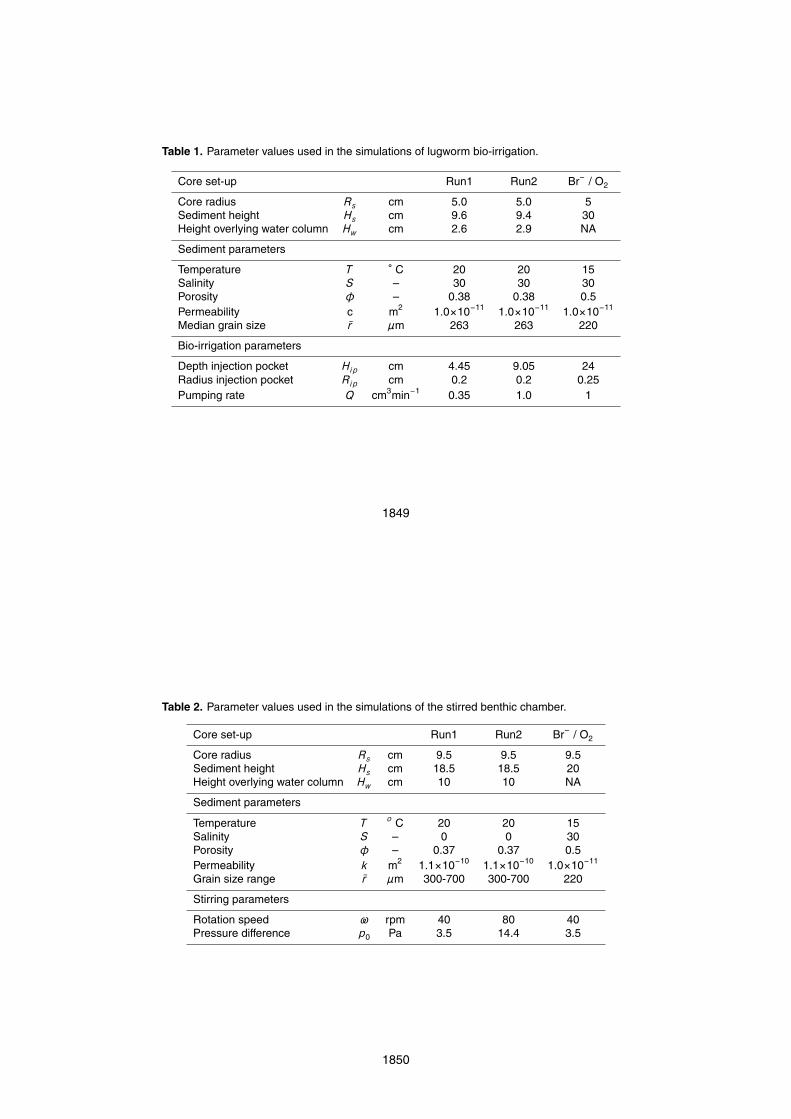
Table 1. Parameter values used in the simulations of lugworm bio-irrigation.

Core set-up Run1 Run2 Br− / O2

Core radius Rs cm 5.0 5.0 5Sediment height Hs cm 9.6 9.4 30Height overlying water column Hw cm 2.6 2.9 NA

Sediment parameters

Temperature T ◦ C 20 20 15Salinity S – 30 30 30Porosity φ – 0.38 0.38 0.5Permeability c m2 1.0×10−11 1.0×10−11 1.0×10−11

Median grain size r µm 263 263 220

Bio-irrigation parameters

Depth injection pocket Hip cm 4.45 9.05 24Radius injection pocket Rip cm 0.2 0.2 0.25Pumping rate Q cm3min−1 0.35 1.0 1

1849

Table 2. Parameter values used in the simulations of the stirred benthic chamber.

Core set-up Run1 Run2 Br− / O2

Core radius Rs cm 9.5 9.5 9.5Sediment height Hs cm 18.5 18.5 20Height overlying water column Hw cm 10 10 NA

Sediment parameters

Temperature T o C 20 20 15Salinity S – 0 0 30Porosity φ – 0.37 0.37 0.5Permeability k m2 1.1×10−10 1.1×10−10 1.0×10−11

Grain size range r µm 300-700 300-700 220

Stirring parameters

Rotation speed ω rpm 40 80 40Pressure difference p0 Pa 3.5 14.4 3.5

1850

Water

Sediment

Burrow

Pore

wat

erfl

ow

Lugworm

Aeration / mixing Water column

Sediment

AquiferGroundwater discharge

Po

rew

ater

flo

w

Lugworm

Water column

Stirrer disk

Sediment

Pore water flow

Overlying water flow

Water column

Sediment

Pore water flow

Fig. 1. Schematic representation of the four situations that are modeled: (a) Laboratory in-cubation set-up commonly used to study lugworm bio-irrigation; (b) Lugworm bio-irrigationinterfering with groundwater seepage on a tidal flat; (c) Pore water flow in stirred incubationchamber; (d) Unidirectional flow over a ripple field inducing pore water flow.

1851

������������������������������������������������������������������������������������������������������

Hp

Hb

Rb

Rc

Hc

�����

�

�

�

�����

Fig. 2. Model [1]: lugworm bio-irrigation in a laboratory core set-up. (a) scheme of the sedimentdomain geometry and the finite element mesh; (b) simulated flow line pattern; (c) simulatedconcentration pattern for the conservative tracer bromide after two hours of flushing; (d) steady-state concentration pattern of oxygen. Concentrations are expressed relative to the constantconcentration in the overlying water column.

1852

������������������������������������������������������������������������������������������������������

� ���

������Fig. 3. Model [2]: interaction between lugworm bio-irrigation and upwelling groundwater on atidal flat. (a) Sediment domain geometry and flow line pattern. The bold dashed line sepa-rates marine conditions (injection of overlying sea water by the lugworm) and fresh conditions(ground water upwelling from below); (b) simulated concentration pattern for the conservativetracer bromide at steady state; (c) steady-state concentration pattern of oxygen. Concentra-tions are expressed relative to the constant concentration in the overlying water column.

1853

�����������������������������������������������������������������������������������������������

� � ��

�

�

��������Fig. 4. Model [3]: pore water flow induced in a stirred benthic chamber. (a) geometry ofthe sediment domain and the finite element discretization; (b) flow line pattern; (c) bromideconcentration pattern after 12 h of incubation with the rotation speed of the stirrer disk set to40 rpm; (d) steady-state oxygen distribution (at 40 rpm). Concentrations are expressed relativeto the constant concentration in the overlying water column.

1854

�����������������������������������������������������������

��

�����������������������������������������������������������������������������������������������������������

� ��

�

�

�

������

Fig. 5. Model [4], laminar variant: Unidirectional flow over a ripple field with laminar flow condi-tions. (a) velocity field in the water column; (b) flow line pattern and bromide distribution after12 h; (c) flow line pattern and steady-state oxygen distribution. Concentrations are expressedrelative to the constant concentration in the overlying water column.

1855

��������������������������������

��

�����������������������������������������������������������������������������������������������������������

� ��

�

�

�

������

Fig. 6. Model [4], turbulent variant: Unidirectional flow over a ripple field with turbulent flowconditions. (a) velocity field in the water column; (b) flow line pattern and the bromide distri-bution after 12 h; (c) flow line pattern and steady-state oxygen distribution. Concentrations areexpressed relative to the constant concentration in the overlying water column.

1856

��������������� �����������

�

���

���

���

���

�

���

� � �� ��

���� ���

�����������������

�

� ��

��������������� �������������

�

���

���

���

���

�

���

� � �� ��

���� ���

�����������������

�

� ��

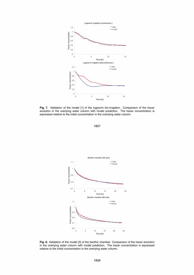
Fig. 7. Validation of the model [1] of the lugworm bio-irrigation. Comparison of the tracerevolution in the overlying water column with model prediction. The tracer concentration isexpressed relative to the initial concentration in the overlying water column.

1857

�������������� ������

���

���

���

�

���

� � �� �� �� ��

���� ���

�������������������

�

� ���

�������������� ������

���

���

���

���

�

���

� � �� �� � �

���� ���

���

����

Fig. 8. Validation of the model [3] of the benthic chamber. Comparison of the tracer evolutionin the overlying water column with model prediction. The tracer concentration is expressedrelative to the initial concentration in the overlying water column.

1858