PERMEABILITY AND MOISTURE DAMAGE …
121
University of New Mexico UNM Digital Repository Civil Engineering ETDs Engineering ETDs 2-14-2014 PERMEABILITY AND MOISTURE DAMAGE CHACTERISTICS OF ASPHALT PAVEMENTS Mohiuddin Ahmad Follow this and additional works at: hps://digitalrepository.unm.edu/ce_etds is esis is brought to you for free and open access by the Engineering ETDs at UNM Digital Repository. It has been accepted for inclusion in Civil Engineering ETDs by an authorized administrator of UNM Digital Repository. For more information, please contact [email protected]. Recommended Citation Ahmad, Mohiuddin. "PERMEABILITY AND MOISTURE DAMAGE CHACTERISTICS OF ASPHALT PAVEMENTS." (2014). hps://digitalrepository.unm.edu/ce_etds/86
Transcript of PERMEABILITY AND MOISTURE DAMAGE …

University of New MexicoUNM Digital Repository
Civil Engineering ETDs Engineering ETDs
2-14-2014
PERMEABILITY AND MOISTURE DAMAGECHARACTERISTICS OF ASPHALTPAVEMENTSMohiuddin Ahmad
Follow this and additional works at: https://digitalrepository.unm.edu/ce_etds
This Thesis is brought to you for free and open access by the Engineering ETDs at UNM Digital Repository. It has been accepted for inclusion in CivilEngineering ETDs by an authorized administrator of UNM Digital Repository. For more information, please contact [email protected].
Recommended CitationAhmad, Mohiuddin. "PERMEABILITY AND MOISTURE DAMAGE CHARACTERISTICS OF ASPHALT PAVEMENTS."(2014). https://digitalrepository.unm.edu/ce_etds/86

i
Student Name: Mohiuddin Ahmad Candidate
Graduate Unit (Department): Civil Engineering Department
This thesis is approved, and it is acceptable in quality
and form for publication:
Approved by the Thesis Committee:
Rafiqul A. Tarefder, Chairperson
Percy Ng, Member
Mark Stone, Member

ii
PERMEABILITY AND MOISTURE DAMAGE CHARACTERISTICS OF
ASPHALT PAVEMENTS
BY
MOHIUDDIN AHMAD
B.Sc. in Civil Engineering
Bangladesh University of Engineering & Technology, Dhaka, Bangladesh
THESIS
Submitted in Partial Fulfillment of the
Requirements for the Degree of
MASTER OF SCIENCE
Civil Engineering
The University of New Mexico
Albuquerque, New Mexico, USA
December 2013

iii
© 2013, Mohiuddin Ahmad

iv
DEDICATION
To my mom

v
ACKNOWLEDGEMENTS
I would like to thank Dr. Rafiqul A. Tarefder for being my advisor and the thesis
committee chair: for his support, time and advice throughout this study. I would also like
to thank my thesis committee members: Dr. Percy Ng and Dr. Mark Stone for their
advice and suggestions during this study.
This study is funded by New Mexico Department of Transportation (NMDOT). I would
like to express my gratitude to Naomi Waterman and Shahidul Amin Faisal for their
continuous support to finish the laboratory experiments. Special thanks go to NMDOT
field exploration team for their help to conduct field testing and sample collection.

vi
PERMEABILITY AND MOISTURE DAMAGE CHARACTERISTICS OF
ASPHALT PAVEMENTS
by
Mohiuddin Ahmad
M.S. in Civil Engineering, University of New Mexico
Albuquerque, NM, USA 2013
B.Sc. in Civil Engineering, Bangladesh University of Engineering & Technology
Dhaka, Bangladesh 2007
ABSTRACT
In the past, numerous studies have been conducted on the topics of moisture damage and
permeability, but very few studies have correlated permeability with moisture damage in
Asphalt Concrete (AC). This study evaluates whether such a relation exists or not. In
addition, correlations of permeability with AC mix volumetrics and pores are evaluated.
Also, correlation of laboratory permeability with field permeability is examined.
In this study, a field survey is conducted to identify a set of eight pavements (bad) that
are known to suffer from moisture damage and a set of eight pavements (good) that do
not exhibit moisture damage. Field permeability testing is conducted on those 16
pavements. Results show that good performing pavements have very low (field)
permeability compared to the bad performing pavements, which was expected. Field
coring is conducted and cores are collected from all 16 pavement sections. Next,
laboratory permeability testing is conducted on the field cores using a falling head
permeameter. Based on laboratory permeability values, the good pavement sections
exhibit smaller permeability than the bad performing sections.

vii
To this end, moisture damage potential of field cores is determined in the laboratory
using Moisture Induced Sensitivity Test (MIST) device and the AASHTO T 283 method.
In MIST method, a sample is wet conditioned using repeated increase and decrease of
pore pressure inside the saturated pores of AC sample. In the AASHTO T 283 method, a
sample is wet conditioned using vacuum saturation and then subjected to one cycle of
freeze-thaw. A set of three wet and three dry conditioned samples are tested for indirect
tensile strength and Tensile Strength Ratio (TSR) of wet to dry sample sets is determined.
It is shown that both MIST and the AASHTO T 283 yield TSR values of less than 1.0,
which means moisture damage occurred by both conditioning methods. Based on the
AASHTO T 283 data, when moisture damage is correlated with laboratory permeability,
the AASHTO T 283 shows a good correlation but MIST shows a poor correlation.
Correlations of field permeability with the AASHTO T 283 and MIST are found to be
poor.
Mix volumetrics (e.g., gradation, porosity, binder content) tests are performed on field
cores. Gradation data is plotted on a 0.45 power curve. Based on the power curve plot, it
is shown that a mix gradation that passes near to the maximum density line have low
permeabilities and moisture damage potentials.
It is known that an AC sample contains 3 types of pore: permeable, dead-end, and
isolated pores. In this study, permeable pore is determined using a tracer test method, a
concept borrowed from soil permeability testing. Dead-end and isolated pores are also
determined using a CoreLok device. It is shown that permeable pores have a better
correlation with permeability than the effective pore, which is defined as the sum of
permeable and dead-end pores.

viii
In this study, an attempt is made to correlate laboratory permeability with field
permeability. Laboratory permeability does not have any correlation with the field
permeability. This may be due to the fact that field permeability is affected by several
factors such as 3D flow in the field, Open Graded Friction Coarse (OGFC), tack coats. To
this end, an analytical model is developed to predict field permeability from laboratory
permeability. Model permeability is found to be higher than the laboratory permeability.
Because the model considers lateral and vertical direction flows whereas laboratory
permeability test considers only vertical flow. It is shown that the model permeability is
less than the field permeability for pavements with OGFC and more than the field
permeability for pavements without OGFC. Therefore, a shift factor is developed to
match the model permeability with the field permeability.

ix
TABLE OF CONTENTS
Abstract .............................................................................................................................. vi
List of Tables ................................................................................................................... xiii
List of Figures .................................................................................................................. xiv
Chapter 1 ............................................................................................................................. 1
Introduction ......................................................................................................................... 1
1.1 Problem Statement .................................................................................................... 1
1.2 Objectives ................................................................................................................. 5
1.3 Organization of the Thesis ........................................................................................ 5
Chapter 2 ............................................................................................................................. 7
Literature Review................................................................................................................ 7
2.1 Introduction ............................................................................................................... 7
2.2 Permeability Test Methods ....................................................................................... 7
2.2.1 Concept of Permeability Testing ....................................................................... 7
2.2.2 Laboratory Methods ........................................................................................... 8
2.2.3 Field Methods .................................................................................................. 12
2.2.4 Arbitrary Methods ........................................................................................... 16
2.3 Factors Affecting Permeability ............................................................................. 17
2.4 Predicting Field Permeability ................................................................................. 17
Chapter 3 ........................................................................................................................... 30

x
Experimental Design ......................................................................................................... 30
3.1 Methodology ........................................................................................................... 30
3.2 Survey ..................................................................................................................... 31
3.3 Field Testing Program............................................................................................. 32
3.4 Test For Mix Volumetrics ....................................................................................... 33
3.5 Laboratory Permeability Testing ............................................................................ 35
3.6 Moisture Damage Test ............................................................................................ 35
3.6.1 AASHTO T 283 Wet Conditioning ................................................................. 36
3.6.2 MIST Wet Conditioning .................................................................................. 36
3.6.3 Tensile Strength Testing .................................................................................. 37
Chapter 4 ........................................................................................................................... 49
Correlating Permeability To Moisture Damage ................................................................ 49
4.1 Introduction ............................................................................................................. 49
4.2 Test Matrix .............................................................................................................. 49
4.3 Results and Discussions .......................................................................................... 50
4.3.1 Mix-volumetric ................................................................................................ 50
4.3.2 Field Damage with Field Permeability ............................................................ 51
4.3.3 Field Damage with Laboratory Permeability of Full Depth Samples.............. 52
4.3.4 Field Damage with Laboratory Permeability of Samples Separated into Layers
................................................................................................................................... 52

xi
4.3.5 MIST Damage with Permeability .................................................................... 53
4.3.6 AASHTO T 283 Damage with Permeability ................................................... 54
4.3.7 Laboratory and Field Permeability .................................................................. 55
4.3.8 MIST and AASHTO T 283 Damage ............................................................... 55
4.3.9 Field Damage with Laboratory Damage .......................................................... 55
4.3.10 Laboratory Compacted Samples .................................................................... 56
4.4 Conclusions ............................................................................................................. 57
Chapter 5 ........................................................................................................................... 75
Field Permeability Model ................................................................................................. 75
5.1 Introduction ............................................................................................................. 75
5.2 Tracer Test .............................................................................................................. 75
5.3 Field Permeability Model ....................................................................................... 77
5.4 Selection of Candidate Pavement ........................................................................... 82
5.5 Results and Discussion ........................................................................................... 82
5.5.1 Different Pores and Their Correlation with Permeability ................................ 82
5.5.2 Laboratory, Predicted and Field Measured Permeability ................................ 84
5.5.3 Quantification of Different Types of Pores and Their Relation with Moisture
Damage ..................................................................................................................... 85
5.6 Conclusions ............................................................................................................. 85
Chapter 6 ........................................................................................................................... 95

xii
Conclusions and Recommendations ................................................................................. 95
6.1 Summary ................................................................................................................. 95
6.2 Conclusions ............................................................................................................. 98
6.3 Recommendations ................................................................................................... 99
References ....................................................................................................................... 100

xiii
LIST OF TABLES
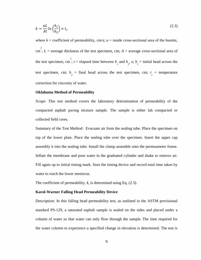
Table 2.1 Different range of permeability and air voids 19
Table 2.2 NMAS and Related Permeability Values 20
Table 3.1 Participation of Districts from NMDOT 38
Table 3.2 Field permeability test locations 39
Table 3.3 Selected Pavements for Laboratory Testing 40
Table 4.1 Test Matrix 58
Table 4.2 Mix data for selected pavements 59
Table 4.3 Permeability Test Results 60
Table 4.4 TSR Calculation 62
Table 5.1 Pavement sections selected for tracer test 87

xiv
LIST OF FIGURES
Figure 2.1 Florida apparatus for permeability 21
Figure 2.2 Karol-Warner falling head permeability device 22
Figure 2.3 TxDOT permeameter 23
Figure 2.4 Pulse-decay permeability measurement 24
Figure 2.5 Kentucky air induced permeameter 25
Figure 2.6 NCAT field permeameter 26
Figure 2.7 ROMUS permeameter 27
Figure 2.8 Kuss Field Permeameter 29
Figure 3.1 Field permeability test set up 41
Figure 3.2 Field permeability test summary for US285 MP 140.53 42
Figure 3.3 Schematic of falling head permeameter 43
Figure 3.4 Different types of pores inside a HMA core sample 44
Figure 3.5 Bulk specific gravity of a cored sample 45
Figure 3.6 Laboratory permeability test 46
Figure 3.7 Sample in the MIST chamber 47
Figure 3.8 IDT testing in progress 48
Figure 4.1 Gradation curve for all pavement sections 64
Figure 4.2 Field permeability at different damage conditions 65
Figure 4.3 Laboratory full depth permeability at different damage
conditions
66
Figure 4.4 Laboratory permeability of separated samples at different
damage conditions
67

xv
Figure 4.5 Correlation of MIST TSR permeability at different modes. 68
Figure 4.6 Correlation of AASHTO T 283 TSR permeability at different
test modes
69
Figure 4.7 Permeability at different test modes 70
Figure 4.8 Comparison between AASHTO T 283 and MIST TSR 71
Figure 4.9 TSR values for good and bad performing pavement sections 72
Figure 4.10 Permeability vs. air voids 73
Figure 4.11 Permeability and moisture damage of labory compacted
samples
74
Figure 5.1 Permeable pores and permeability set up 88
Figure 5.2 Breakthrough curve for a sample from NM344 at MP1.8 89
Figure 5.3 Different types of pores in a sample 90
Figure 5.4 Different types of pores and their correlation 91
Figure 5.5 Different permeabilities and their relation with pores 92
Figure 5.6 Comparison of field permeability with predicted and laboratory
permeability
93
Figure 5.7 Different types of pores and their relation with moisture
damage
94
1
CHAPTER 1
INTRODUCTION
1.1 PROBLEM STATEMENT
In the past, New Mexico Department of Transportation (NMDOT) has built asphalt
pavements using dense-graded Hot Mix Asphalt (HMA) mixes. The initial in-place total
pores (voids) of those dense graded mixtures are controlled not to be higher than eight
percent and never fall below three percent during the life of the pavement. Higher pore
content makes the pavement structure more permeable to air and water. High
permeability may cause enhanced aging and moisture damage of HMA as well as
endanger the subgrade and base courses. Lower pore content causes rutting and shoving
due to shear deformation of mix constituents under repeated traffic loading. Thus, pores
in an asphalt concrete pavement have contrasting effects on its properties and
performance. Studies have shown that a dense graded mix containing total pores below
8% has low permeability (less than 100 x 10-5
cm/sec), which prevents infiltration of
water inside a pavement (Mallick et al. 2001, Cooley and Brown 2000, Daniel et al.
2007). As a result, very little to no attention has been given so far to permeability of
dense graded asphalt mixes nationally and in the state of New Mexico. This study
determines permeability of sixteen pavement sections in New Mexico.
Moisture damage of asphalt pavement is an important issue worldwide. In the United
States, the problem is also severe, as 34 out of 50 states are suffering from some sort of
moisture related distress (Hicks 1991). According to Mogawer et al. (2002), 15 states
reported moisture related problems out of 27 states surveyed. Moisture can enter inside

2
the pavement by three ways: infiltration, evaporation and capillary rise (Mercado 2007).
In all cases, permeable pores provide the pathway for water to get inside the pavement.
Moisture damage in asphalt can be prevented either by preventing water from entering an
asphalt concrete (AC) or by strengthening the AC materials in the asphalt-aggregate
system. Permeability is the way by which water can enter inside the pavement. This study
evaluates whether the moisture damage in AC may be prevented or reduced by
controlling permeability.
Very few studies have been conducted correlating permeability and moisture damage to
this day. Choubane et al. (2007) has related degree of saturation with moisture damage.
Moisture damage increases with the increase of saturation. Torres (2004) and Masad et
al. (2006) divided air void content into three categories: low (impermeable), pessimum
(intermediate) and free drainage. Maximum damage occurs at the intermediate range of
permeability which corresponds to pessimum air void content. However, this has not
been verified for different field conditions and test methods. Moisture damage of a
pavement can be evaluated by two ways: visual inspection and mechanical testing.
Stripping, which is one of the most common forms of moisture damage, generally occurs
at interfaces and propagates upward. Therefore, it is difficult to identify moisture damage
by visual inspection only (Kim and Coree 2005). Mechanical methods used are the
AASHTO T 283 (AASHTO 2007), Moisture Induced Sensitivity Testing (MIST),
Nottingham asphalt test equipment, Hamburg wheel test, etc. Among them, the AASHTO
T 283 is the most widely used and experimented method. In the AASHTO T 283 method,
samples are vacuum saturated and subjected to freeze-thaw. However, it is time
consuming and the variable degree of saturation may affect the test result. The pore

3
pressure cycles, as in the field due to wheel passing on moist pavement, are not simulated
in this method (Liang 2008). The recently developed MIST device can simulate pore
pressure cycles (MIST 2012). In this study, both the AASHTO T 283 and MIST are used
to cause moisture damage to AC samples in the laboratory.
Past studies show that permeability increases exponentially with the increase in total
pores in HMA samples (Retzer 2008, Mallick et al. 2003, Vivar and Haddock 2007,
Cooley et al. 2002, Hainain et al. 2003, Ahmad and Tarefder 2013). Total pore consists of
three pores: permeable pore, dead-end pore, and isolated pore (Tarefder and Zaman
2005). Only pores that continue from the top to the bottom of a sample are responsible
for permeability (i.e., conduction of flow) and therefore they are called permeable pores.
Permeable pores and dead-end pores are accessible by water and therefore, sum of these
two pores are also known as effective pores (Bear 1972). Effective pore in an AC sample
is always less than the total pores (Koponen et al 1997). Effective pores can be
determined using a CorelokTM
device as per ASTM D 6752. In fact, CorelokTM
device
measures both bulk and apparent specific gravities. The percent difference in specific
gravities normalized by the apparent specific gravity gives the effective pores (Vivar and
Haddock 2005, Bhattacharjee and Mallick 2002). In the past, most studies concluded that
a poor correlation exists between the total pore and permeability. Permeability
specifications of some state Department of Transportation (DOTs) are also based on the
total pores and permeability correlation. Some studies have shown that effective pores
show a better correlation with permeability (Bear 1973, Bhattacharjee and Mallick 2002),
as isolated pores are eliminated from total pores. However, effective pores include dead-

4
end pores, which have little or no contribution to permeability (Bear 1973). Ideally, one
should correlate permeable pores to permeability.
As flow occurs only through permeable pores, it is necessary to measure it, which is done
in this study. Ranieri et al. (2010) determined pores using X-ray tomography and
correlated it to permeability. Liang et al. (2000) used image processing to determine
pores in rocks. Omari (2004) used X-ray CT images to evaluate pores of HMA cores.
While these methods are very advanced and sometimes complex, a tracer method, which
has been successfully used for soils permeability (Rogowski 1988, Yeh et al. 2000,
Stephens et al 1998), can be useful and therefore tried in this study to determine
permeable pores in AC.
Although permeability of HMA pavement is measured both in the field and laboratory,
correlating laboratory permeability with field permeability is very difficult. In the
laboratory, permeability test sample confined at the sides and flow is regulated one-
dimensionally, which is different from the field permeability boundary condition. Some
researchers tried to correlate laboratory permeability to field permeability (Keniptong et
al 2005), but those studies did not succeeded and were based on experiments only. Field
permeability is affected by several variables such as degree of saturation, boundary
conditions, flow directions, etc. (Gogula et al 2004). Thus field measured permeability
value is always found to be either less or more than the laboratory permeability of AC
sample. For example, during field permeability testing in this study, it was clearly
observed that if a field HMA layer is covered by an Open Graded Friction Course
(OGFC), water mostly flow laterally through the OGFC layer during field permeability
testing. Water flow through the OGFC yields a very high permeability, which is not the

5
representative permeability of the HMA layer. In other cases, if field HMA layers contain
a seal coat, tack coat, and prime coat, these coats retard the vertical flow during field
permeability testing and yield a very low permeability, which is also not the true
permeability of the HMA layer. Therefore, field permeability test results need to be
evaluated cautiously. Saturation is another issue but needed for a successful permeability
testing in the field. One can use air permeameter, which can eliminate the problem
associated with degree of saturation to some degreed (Menard and Crovetti 2006).
However, it still has other limitations such as different coatings and boundary conditions.
In addition, sometimes it is difficult to set up field permeability tests due to bad weather,
a lack of field crews, and required traffic control. This study attempts to develop an
analytical model to predict field permeability from laboratory core permeability test
results.
1.2 OBJECTIVES
The main objectives of this study are to:
Find whether permeability is related to moisture damage of AC.
Measure permeable pores in AC and its relation to permeability.
Relate field permeability with laboratory permeability.
1.3 ORGANIZATION OF THE THESIS
This thesis consists of six chapters. Chapter 1 defines the problem of permeability and
moisture damage in AC. Chapter 2 contains literature review on different laboratory and
field permeability test methods, factors affecting permeability, permeability practices of
different states and countries. Chapter 3 contains experimental plan for this study, field

6
and laboratory testing performed during this study. Chapter 4 describes the correlation
between permeability and moisture damage. Chapter 5 determines the permeable pores
and an analytical model to determine field permeability from testing cores in the
laboratory. Chapter 6 summarizes the findings of this study.

7
CHAPTER 2
LITERATURE REVIEW
2.1 INTRODUCTION
The author conducted a comprehensive search of databases and various information
sources (like journals, research reports, standards) to build a solid base of knowledge on
current research. Particular emphasis was placed on permeability testing methods.
Review of the factors affecting permeability is also made.
2.2 PERMEABILITY TEST METHODS
2.2.1 Concept of Permeability Testing
Permeability or hydraulic conductivity of a material refers to its ability to transmit water
through it. It is obtained from Darcy’s law: flow velocity is proportional to hydraulic
gradient.
(2.1)
where V = flow velocity (cm/s); i = flow gradient defined by head loss over sample
length; k = permeability of the sample (cm/s).
Therefore, discharge rate (Q) will be:
(2.2)
where Q = discharge (cm3/s) and A = cross section area (cm
2).

8
Permeability of soil is determined either using falling head or constant head
permeameter. Almost all permeameter are based on one of these two mechanisms.
Permeability of asphalt is evaluated both in the field and in the laboratory. Different
states or organizations used different instruments to determine permeability. Brief
descriptions of them are given in next sections.
2.2.2 Laboratory Methods
Florida Method of Permeability
Scope: This test method covers the laboratory determination of the water conductivity of
compacted asphalt paving mixture sample. The measurement provides an indication of
water permeability of that sample as compared to those of other asphalt samples tested in
the same manner. The procedure uses either laboratory compacted cylindrical specimens
or field core samples obtained from existing pavements.
Summary of the Test Method: A falling head permeability test apparatus is used to
determine the rate of flow of water through the specimen. Water in a graduated cylinder
is allowed to flow through a saturated asphalt sample and the interval of time taken to
reach a known change in head is recorded. The coefficient of permeability of the asphalt
sample is then determined based on Darcy’s Law.
Significance and Use: This test method provides a means for determining water
conductivity of water-saturated asphalt samples. It applies to one-dimensional, laminar
flow of water. It is assumed that Darcy’s law is valid.
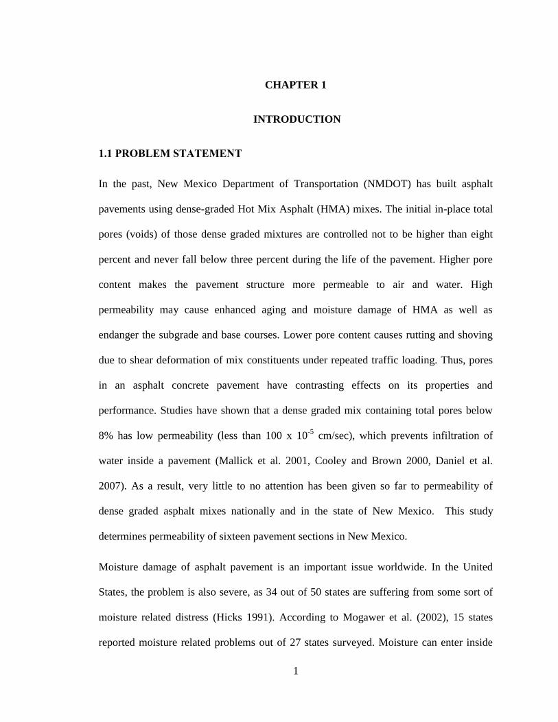
Calculations: The coefficient of permeability, k, is determined using the following
equation:
9
(
)
(2.3)
where k = coefficient of permeability, cm/s; a = inside cross-sectional area of the burette,
cm2
; L = average thickness of the test specimen, cm; A = average cross-sectional area of
the test specimen, cm2
; t = elapsed time between h1
and h2, s; h
1 = initial head across the
test specimen, cm; h2
= final head across the test specimen, cm; tc
= temperature
correction for viscosity of water.
Oklahoma Method of Permeability
Scope: This test method covers the laboratory determination of permeability of the
compacted asphalt paving mixture sample. The sample is either lab compacted or
collected field cores.
Summary of the Test Method: Evacuate air from the sealing tube. Place the specimen on
top of the lower plate. Place the sealing tube over the specimen. Insert the upper cap
assembly it into the sealing tube. Install the clamp assemble onto the permeameter frame.
Inflate the membrane and pour water in the graduated cylinder and shake to remove air.
Fill again up to initial timing mark. Start the timing device and record total time taken by
water to reach the lower meniscus.
The coefficient of permeability, k, is determined using Eq. (2.3).
Karol-Warner Falling Head Permeability Device
Description: In this falling head permeability test, as outlined in the ASTM provisional
standard PS-129, a saturated asphalt sample is sealed on the sides and placed under a
column of water so that water can only flow through the sample. The time required for
the water column to experience a specified change in elevation is determined. The test is

10
repeated until four consecutive readings do not differ by more than ten percent. This
process confirms that the sample was, in fact, saturated. Otherwise, it would be
unclear whether movement of the water column was due to water infiltrating void spaces
or actual flow through the sample (Williams, et al. 2006).
Calculation: The permeability for water is calculated using the following equation,
(
) (2.4)
TxDOT Permeability Method
Scope: This test procedure to measures the time of water flow through laboratory
compacted specimens. Then permeability is determined.
Apparatus: Cylindrical laboratory permeameter, stop watch.
Specimen: 6 in. diameter 4.5 in. height lab compacted sample or field core of 6 in.
diameter and height not more than 4.5 in.
Procedure: The test specimen is placed inside the cylindrical laboratory permeameter.
Rubber clamps around the permeameter are secured at the top and bottom edges of the
test specimen. The clamps are placed such that the top and bottom edges are
approximately in the middle of the location of the clamps. The permeameter is filled with
water approximately 1–2 in. above the top marking on the pipette. The timing device is
started when the water level reaches the top marking on the pipette. The timing is stopped
when the water level reaches the bottom marking on the pipette. The time taken by water
to travel from the top marking to the bottom marking is recorded. Permeability is
calculated by falling head formula.

11
Pulse-Decay Method of Permeability
Introduction: The system consists of an upstream reservoir of volume V1, a sample holder
and a downstream reservoir of volume V2. A differential pressure transducer measures the
pressure difference between the reservoirs and another transducer measures the pressure
p2 in the downstream reservoir. No flow measurement device is required. Flow rate can
be calculated from known volume of each reservoir, fluid compressibility and rate of
pressure change.
Procedure: High pressure is applied at upstream reservoir with all bulbs open. When
pressure become uniform all over the system, upstream pressure is increased keeping
bulbs such way that pressure pulse enters into the sample. The upstream pressure will
decrease with time and downstream pressure will increase until the pressure difference
become zero. The pressure difference is measured with time and plotted in a semi-log
plot. The slope of the line could be obtained by:
| |
(
)
(2.5)
Hence,
(
)
(2.6)
where m = slope; µL = viscosity of the liquid, cp; cL = liquid compressibility, psi-1
; cv1 =
compressibility of upstream reservoir, psi-1
; f1 = mass-flow correction factor; A = cross
section area of the cylindrical sample, cm2.
This method is used normally for rock permeability measurement.

12
Faster Pulse Decay Permeability Measurement
Description: The method is similar to that described in previous method, except the
pressure equilibrium step is eliminated and the test can be performed quicker than before.
And two additional reservoirs are added to the previous instrument.
2.2.3 Field Methods
California Method of Permeability
Scope: This method describes the procedure for determining the permeability of
bituminous pavements and seal coats.
Test Procedure: A 6 in. diameter circle on pavement surface is drawn, small amount of
grease is pushed on pavement, and cylinders are filled with test solution. The valve at the
base of the special plastic graduated cylinder is released. The special plastic cylinder is
refilled from the polyethylene graduate if more solution is needed during the test. At the
end of the 2-minute test period, the total amount of solution used is determined.
Calculation: The total quantity of solution used during the test period is divided by two
and the result is shown as the relative permeability in mL/min.
Kentucky Method
Scope: This method describe the procedure for determining in place permeability of an
HMA mat using an air induced permeameter. This method is applicable for all nominal
maximum size and gradation.
Apparatus: Permeameter, Air compressor and caulking gun.
Procedure: The air compressor is connected to the multi venture vacuum cube.
Approximately a one-half inch bead of silicon rubber caulk is applied; one inch inside the
outer edge of sealing ring. The permeameter is placed in the center of the area to be

13
tested. No more than 50 pounds of load is applied on permeameter and twist. The bulb of
multi-venturi vacuum cube is opened to permit the flow of air. The reading on the digital
vacuum will begin to increase. When this number reaches to peak, the test is finished and
the bulb can be shut. Test time should not exceed 15s. The highest reading attained by the
permeameter is recorded by pressing the button marked “HI/LO”.
Calculation: Permeability of the mat in ft/day may be calculated from the following
equation,
(2.7)
where k = permeability in ft/day; V = vacuum reading in mm Hg
TxDOT Procedure for Field Permeability
Scope: This empirical test procedure is used for pavements under construction or on
roadways already constructed to test and verify that the compacted mixture has adequate
permeability.
Apparatus: Cylindrical field permeameter, stop watch and Plumber’s putty.
Procedure: The permeameter is placed on the pavement surface using putty to seal it with
pavement. The permeameter is filled 1-2 inch more than top marking. Time taken by
water to travel from tom marking to bottom marking is recorded. Time is normally less
than 20s for newly constructed pavement. Permeability is calculated using falling head
method.
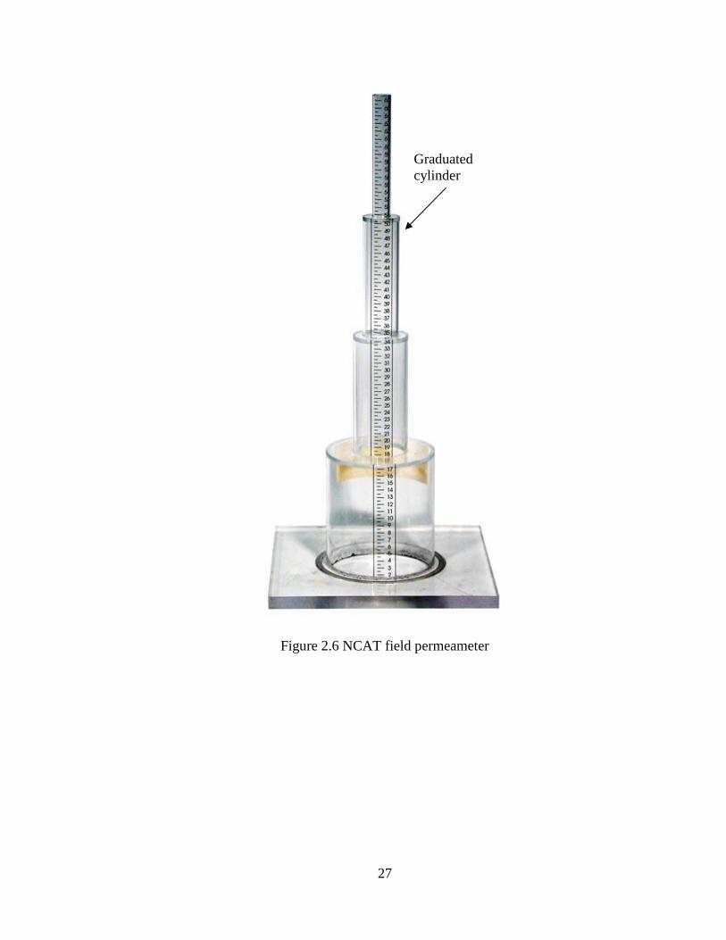
NCAT Field Permeameter
Scope: This test method covers the in-place estimation of the water permeability of
compacted hot mix asphalt (HMA) pavement.

14
A falling head permeability test is used to estimate the rate at which water flows into a
compacted HMA pavement. Water from a graduated standpipe is allowed to flow into a
compacted HMA pavement and the interval of time taken to reach a known change in
head loss is recorded. The coefficient of permeability of a compacted HMA pavement is
then estimated based on Darcy’s Law.
Significance and use: This test method provides a means of estimating water
permeability of compacted HMA pavements. The estimation of water permeability is
based upon assumptions that the sample thickness is equal to the immediately underlying
HMA pavement course thickness; the area of the tested sample is equal to the area of the
permeameter from which water is allowed to penetrate the HMA pavement; one-
dimensional flow; and laminar flow of the water. It is assumed that Darcy’s law is valid
(Cooley et al. 1999).
Calculation: Same formula used for any falling head method.
ROMUS Air Permeameter
Description: The ROMUS air permeameter uses air that is gathered from the atmosphere
as the fluid to measure permeability. The machine has a vacuum pump that operates on a
rechargeable battery and depressurizes the tank to negative 24 inches of head. When the
test is ready to begin, the air tank is pressurized to 24 inches of head if it is not already at
the appropriate pressure. The air is then drawn through the pavement surface while a
pressure sensor checks the pressure in the tank. At every 4 inches of pressure drop the
time is recorded. The time is the only output for the device (Retzer et al. 2008).
Calculation: Permeability of the pavement is calculated from the following equation
which is modified from falling head equation:

15
[
] (
) (2.8)
where kw = hydraulic permeability ,cm/s; L = pavement layer thickness cm; V = volume
of vacuum chamber (cm3); μ = kinematic viscosity of air (gm/cm/s); ρw = density of
water (gm/cm3); g = gravitational acceleration (cm/s
2); T = time of head drop (s); A =
area of being tested (cm2); Pa = pressure (atmospheric) (Ba); μw = kinematic viscosity of
water (gm/cm/s); p1 = initial pressure (Ba); p2 = final pressure (Ba).
The Kuss Field Permeameter
Description: The Kuss Field Permeameter (KSFP) operates using the constant head
approach. To do this, a patented gas-measurement system is used to measure the amount
of air needed to replace the water in order to maintain a constant pressure head. When
the test begins, water is allowed to flow from the standpipe and cover the pavement
testing surface to a depth of approximately 1 in. A sensor is used to monitor the water
level, and is connected to a flow valve in the flow meter box. As water infiltrates the
pavement, the water level over the pavement drops, and the sensor alerts the flow valve,
allowing air to enter the standpipe above the water column. This metered volume of air
acts as a substitute for the head pressure originally applied by the water, thereby
maintaining a constant head. A data acquisition system measures and records the flow
rate of water through the pavement over time, and the permeability is calculated using the
rate of flow of water into the pavement and the cross-sectional area of the pavement test
section. The relationship is presented in Equation below, (Williams et al. 2006):
(
)
(2.9)

16
where k = coefficient of permeability, cm/s; Q = flow rate, cm3/min; A = area of base
plate, 1264.5cm2; L = pavement thickness, cm.
Double Ring Infiltrometer
The double ring infiltrometer test is performed as per ASTM D 3385 and mainly used for
soils. Two 20 in. high ring of 12 in. and 24 in. diameter are used. The rings are driven to
the soft ground around 6 in. Water flow by the outer ring forces the water flow through
inner ring in perpendicular direction only. The infiltration rate of the inner tube is
measure. However, it is difficult to use the infiltrometer for asphalt pavements as it can’t
be driven inside the pavement.
2.2.4 Arbitrary Methods
Modified Kozeny-Carman equation
(2.10)
where % air void; γ = 9.79 kN/m3; µ = fluid viscosity. (Masad et al. 2002)
The permeability coefficient of an asphalt mixture can be estimated by the following
equation (Arkansas Highway Transportation Department (1998)):
(2.11)
where %Va = Air Voids, expressed as a percentage; t = lift thickness (Willoughby, et all.
2001).

17
2.3 FACTORS AFFECTING PERMEABILITY
Research conducted by the NCHRP showed an inverse relationship between VMA and
mixture permeability, i.e. for a given air void content permeability decreased as the VMA
increased (Brown et al. 2004). Also, with increase in coarse aggregate, permeability also
increased. One reason for such increase is increase of interconnected air voids. Superpave
mixes tend to have this trait as well as having a larger NMAS with lesser fines to fill void
spaces which results in a substantial increase in permeability (Vivar 2007). Void
contents as low as 4.4% have been shown adequate for 25 mm NMAS mixes and 7.7%
being the maximum for NMAS mixes of 9.5 mm. Table 1 shows air permeability ranges
at different air voids.
Permeability increases with an increase of NMAS. Mallick et al.2003 got permeabilities
for 6 percent air void as shown in Table 2.
Another factor that influences permeability is gradation. For coarse graded mix, because
of coarser particles, the void size is larger resulting more interconnected void. According
to Mallick et al, lift thickness (or t/NMAS) also affects permeability. As thickness (or
t/NMAS) increases, the potential for interconnected air void decreases, resulting
decreases in permeability.
2.4 PREDICTING FIELD PERMEABILITY
Kanitpong et al. (2005) performed many field tests for permeability and lab test of lab
compacted sample of same mix design to relate field and lab permeability value. He also
correlated field permeability by field test method with field permeability by lab test. He
gave the following correlation of field permeability and lab permeability of field cores:

18
(2.12)
(2.13)
where P8 is the percent passing through No.8 sieve. No correlation was found for other
mixtures.
To determine correlation between field permeability with lab compacted sample
permeability, he described two methods.
Method A: First, Gmb of field core is determined. Then amount of material needed to
produce lab sample of same height and density were determined using the following
equation,
(2.14)
where Wt = amount of material, gm; t = height or thickness of the field cores, mm; A =
cross section area of the specimen, mm2.
The SGC sample was compacted using the Superpave Gyratory Compactor, fixing the
height. The permeability of these samples were predicted and found less than that
obtained from field cores. And the relation is described by:
R2 =0.6 (2.15)
where y = lab permeability of field cores (cm/s); x = lab permeability of SGC sample
(cm/s).
Method B: Here mixes are collected from field and Ndes was fixed for all samples. So,
densities of the samples were different. Then, permeability of the samples was

19
determined using ASTM D5084. And permeability vs. density curve was plotted for SGC
samples of method B. From this plot, permeability corresponding to field density was
determined. Finally, predicted permeability and measured permeability of field cores
were plotted on a graph which gives almost a straight line of slope 1. That indicates the
Permeability determined by method B was equal to the permeability of field cores.
20
Table 2.1 Different range of permeability and air voids
k (cm/s) Description of Permeability Description of Air Voids
<10-4
Impervious-Impermeable <5%
10-4
-10-2
Poor drainage-Permeable 5-7%
10-2 or higher Good Drainage-Very
Permeable
>7%

21
Table 2.2 NMAS and related permeability values
NMAS(mm) Permeability(cm/s)
9.5 6 x 10⁻⁵
12.5 40 x 10-5
19.0 140 x 10-5
25.0 1200 x 10-5

22
Figure 2.1 Florida apparatus for permeability

23
Figure 2.2 Karol-Warner falling head permeability device

24
Figure 2.3 TxDOT permeameter
Pipette marking
for measuring
time
Pipett
e

25
(a) Pulse-decay measuring apparatus
(b) Faster pulse-decay measuring apparatus
Figure 2.4 Pulse-decay permeability measurement

26
Figure 2.5 Kentucky air induced permeameter
27
Figure 2.6 NCAT field permeameter
Graduated
cylinder

28
Figure 2.7 ROMUS permeameter
Vacuum Pump
Air Tank of Known Volume
Pressure
Sensor
Timing
Device
Check Valve
Seal to Pavement
Asphalt Surface
Main Valve

29
Figure 2.8 Kuss field permeameter

30
CHAPTER 3
EXPERIMENTAL DESIGN
3.1 METHODOLOGY
The experimental plan for this study is shown in Figure 3.1. A field survey was
conducted in cooperation with New Mexico Department of Transportation (NMDOT).
The main objective of the field survey was to identify a set of bad (moisture damaged)
and good (undamaged) performing asphalt pavement sections.
Field permeability tests were performed on those sections using an NCAT field asphalt
permeameter. In New Mexico, most of the pavements are surfaced with open graded
friction course (OGFC). Therefore, permeability testing and field coring were conducted
on the shoulder, which is not typically treated with OGFC.
Florida apparatus using the falling head permeability test method determined laboratory
permeability values of full depth cores. Ideally, full depth laboratory permeability should
be compared to field permeability. The cores were separated by layers using a laboratory
wet saw. Permeability tests were performed on the samples representing individual
layers.
Moisture damage on samples separated by layers was evaluated by a ratio of the indirect
tensile strength of a set of wet samples to that of a set of dry samples. In this study, wet
conditioning was performed by two methods: the AASHTO T 283 (AASHTO 2007) and
a recently developed MIST device. The difference between the AASHTO T 283 and
MIST conditioning is that the AASHTO T 283 causes damage to the AC sample by

31
freeze-thaw action and MIST causes damage to the AC sample by increasing and
releasing pore pressure inside the sample. In both cases, temperature is 60 °C.
3.2 SURVEY
The survey questioner was set by the distributed to 42 NMDOT employees from all six of
the NMDOT districts. The survey was followed by phone calls to spur the response.
Below are the two questionaries’ of the survey.
Is there a section (or project) of a roadway/pavement that shows moisture wicking
in your district? Basically, if you know about a pavement section that does not get
dried up in few hours (say couple of hours) after a short rainfall. If such, what is
causing the above problem (high permeability, stripping, roadway drainage
problem, moisture damage, etc.)?
Can you mention couple of pavement sections that are performing very well in
terms of permeability or drainage or moisture damage or stripping issue? Milepost
or location will be helpful.
Survey Response Synthesis and Data Collection
Except district 1 and 4, all other four districts answered the survey questions. Based on
their answers, pavements with high permeability or showing visual stripping are
classified as bad performing pavement. On the other hand, pavements with low
permeability or no visual stripping are grouped as bad performing pavements. List of
good and bad performing sections are shown in Table 3.1.

32
3.3 FIELD TESTING PROGRAM
Based on the survey, field permeability tests were performed on the locations shown in
Table 3.2.
Procedure for the field testing followed by the UNM research team includes a field
inspection of drainage, measurement and sketch of the lane markings and characteristics
of the section including width of lanes, shoulder, wheel path location and distance from
the shoulder stripe. The drainage is determined by the measurement of the slope and
inspection of the crown design. The team then lays down a template around the tape
marks from the FWD testing that the NMDOT team has performed at the section
location. The holes are marked with construction crayon and the team determines which
will be used for field testing and proceeds to testing. After the tests are performed, the
NMDOT team cores the 24 holes that were marked by the UNM research team. 12 6”
diameter cores and 12 4” diameter cores were taken and cataloged by the NMDOT team.
Figure 3.1 shows the field permeability test set up. Figure 3.2 show schematics of a
section from District 2 that were tested March 14-15, 2012. Figure 3.3 describes the
falling head permeability mechanisms.
NCAT field asphalt permeameter is used to determine field permeability value using Eq.
(2.4).
In the field, a crack-free spot is selected to place the permeameter. This area is then
cleaned using a broom. Next, a wax ring is placed at the base of the permeameter, which
is then placed on the cleaned area. The base is pushed downward so that the wax ring is
attached to the pavement without any water leaking. Three 10 lb. weights are then placed
on the permeameter base to resist it from uplift pressure by water. Water is poured inside

33
the tube and it is allowed to flow for a few minutes to saturate the pavement. Figure 3.1
shows a field permeability test set-up. Though Eq. (2.4) is used for field permeability
value, flow occurs both in vertical and lateral directions in the field. An impermeable or
incompatible middle layer can direct the flow along the lateral direction. The
permeability test was conducted around noon time. It is possible that a thermal gradient
exists along the thickness of the Hot Mix Asphalt (HMA) pavements, which may affect
the flow. However no temperature correction is considered for field permeability
calculations.
Core Collection and Selection of Candidate Pavements for Laboratory Testing
A total of 24 cores were collected from each of the 23 locations. The cores were
inspected to see if there exists any stripping at the interface of the layers. Depending on
the visual inspection the pavements were classified as good or bad performing as shown
in Table 3.3. The number assigned to each pavement and number of layer each pavement
has are also shown in this table.
3.4 TEST FOR MIX VOLUMETRICS
The total air void a sample has is termed as total pores. It consists of permeable pores,
isolated pores, and dead end pores. Permeable pores and dead end pores are accessible by
water and termed as effective pores. These pores are shown in Figure 3.4.
Bulk specific gravity of a cored sample is determined using CorelokTM
device as per
ASTM D 6752. Dry weight of the sample is measured. Sample is placed inside a plastic
bag of known weight and specific gravity and placed inside the CorelokTM
device. Air
from the Corelok chamber is sucked out and the polybag is sealed as shown in Figure 3.5.

34
The underwater weight of the sample with polybag is measured. The bag is cut open
under water and the weight is recorded again. Bulk specific gravity of the sample is
calculated from Eq. (3.1):
(3.1)
where A = sample dry weight in air, gm; D = polybag weight in air, gm; B = weight of
sealed sample in water, gm; F = specific gravity of polybag at 25 °C.
Apparent specific gravity is determined using Eq. (3.2):
(3.2)
where C = weight of sealed sample and polybag cut under water.
Effective pores are determined using Eq. (3.3) as follows:
(3.3)
After all tests are done on a sample, it is placed inside the oven to prepare loose mix.
Maximum specific gravity is determined using Corelok device as per ASTM D6857.
Weight of loose mix and polybag is measured. The loose mix is placed inside the polybag
and vacuum sealed. The bag is cut opened under water and water saturates the mix. The
weight is measured. Maximum specific gravity is then determined by Eq. (3.4):
(3.4)
A = loose mix dry weight in air; D = polybag weight in air; C = weight of saturated
sample and polybag in water; F = specific gravity of polybag at 25 °C.

35
Finally, total pores are determined using Eq. (3.5) as follows:
(3.5)
3.5 LABORATORY PERMEABILITY TESTING
Florida apparatus was used for laboratory permeability measurement. It is repeatable,
available, and easy to use. Flow in this permeameter is one-dimensional. It uses Eq. (2.3).
Figure 3.6 shows the permeability test set-up in the laboratory. Both ends of the cored
sample are smoothed using a wet saw. Before placing a sample in the laboratory
permeameter, it was saturated using CorelokTM
device. In CorelokTM
, a sample is vacuum
sealed in a plastic bag, which is cut open under water to saturate the sample. This method
has shown to be more effective than flask-vacuum saturation (Tarefder et al. 2002).
Petroleum jelly is applied on the curve surface of the sample to make lateral surface
impermeable and to have a good seal so that no water flow through the interface of
sample and permeameter. The sample was then placed inside a cylinder enclosed by a
membrane and pressurized to confine the side so that water flows in vertical direction
only. Temperature of the water is recorded. Water level was recorded at different time
interval.
3.6 MOISTURE DAMAGE TEST
Moisture damage is measured by the ratio of wet to dry sample’s IDT. For dry
conditioning, the dry sample was placed inside a Ziploc bag and placed under water at 25
°C (77 °F) for two hours. For wet conditioning, the AASHTO T 283 method and MIST
devices were used.

36
3.6.1 AASHTO T 283 Wet Conditioning
In the AASHTO T 283 method, an asphalt core is saturated using a vibro-deairator device
that applies vibration and suction simultaneously. After saturation, the sample is placed
inside a moist Ziploc bag and placed in a refrigerator for 16 hours at -23 °C (0 °F) for
freezing. The sample is thawed in a hot water bath at a temperature of 60 °C (140 °F) for
24 hours followed by two hours of conditioning at 25 °C (77 °F) (24). Thus, in the
AASHTO T 283 conditioning process, water is forced to enter inside the sample during
saturation and to increase in volume during freezing. The increased volume of water
causes increased pressure inside the pores of the sample causing damage. Thawing by hot
water for 24 hours also contributes to the softening of the binder, mastic and samples.
3.6.2 MIST Wet Conditioning
In this method, a core sample is placed inside the MIST chamber filled with water as
shown in Figure 3.7. A bladder inside the watertight chamber is used to increase and
decrease the chamber pressure. In this study, the chamber temperature was set at 60 °C
(77 °F) with a chamber pressure of 40 psi. A total of 3500 cycles of pressure increase and
release were applied to the cored samples. As the number of cycles increase, the air
inside the sample is replaced gradually with water. At certain cycles of intervals, air
bubbles are released through the opening of the top of the chamber lid. Water inside the
pores is pressurized to cause damage in the cores. After completion of MIST
conditioning, the sample is placed under water at room temperature for about 2 hours for
further conditioning.

37
3.6.3 Tensile Strength Testing
Dry and wet conditioned samples are loaded diametrically to fail in tension as shown in
Figure 20. The load is applied at 50 mm/min rate and the peak value of the load is
recorded. The indirect tensile strength is calculated using Eq. (3.6):
(3.6)
where IDT = indirect tensile strength (kPa); P = peak force needed to crack the sample
diagonally, recorded from the compression testing device (Newton); D = diameter of the
sample (cm); L = length of the sample (cm).
Tensile Strength Ratio (TSR) of wet to dry samples is calculated using Eq. (3.7):
(3.7)
where IDTwet = Average IDT of three wet conditioned samples, IDTdry = Average IDT of
three dry conditioned samples.

38
Table 3.1 Participation of districts from NMDOT
District Low Permeability/ Good performing
Pavement
High Permeability / Bad
performing Pavement
District 2 US 285 MP 115-MP 205 US 70 MP 268 - MP 301
District 3 I-40 from Coors to Unser I-25 from south of Budaghers
north to Santa Fe county line
(District 3 boundary)
District 6 C.N. ESG5B66, US 491, M.P. 59.0 –
67.7, San Juan County
I-40 mile markers 18 – 22
C.N. G1436ER, I-40, M.P. 126.2 –
130.7, Cibola County
C.N. 6100430, NM 264, M.P.
10.6 – 13.1, McKinley County,
Roadway Rehab with WMA
Dist. 5 US 285, MP 284 – 290
NM 14, MP 47 - 50
US 84, MP 233 – 238
NM 344, NM 2 – 14

39
Table 3.2 Field permeability test locations
Pavements Location
US285 MP126.23
MP140.53
MP152
MP285.25
MP285.5
US70 MP289.26
MP282.2
MP272.67
US491 MP60.9
MP60.5
MP60.7
I40 MP335.5
US264 MP10
MN14 MP46.80NB
MP46.80SB
MP46.9SB
NM344 MP1.80
MP1.82
MP1.84
US84 MP235.8
MP235.9
MP236
I40 MP23.1

40
Table 3.3 Selected pavements for laboratory testing
Good Performing Pavements
(Not showing Moisture Damage)
Bad Performing pavements
(Showing Moisture Damage)
Pavement location ID Number
of layers
Pavement location ID Number
of layers
US285 MP126.3 1 2 US70 MP289.26 9 3
US285 MP285.25 2 3 US70 MP282.2 10 3
NM344 MP1.80 3 1 US70 MP272.67 11 3
NM14 MP46.8 4 3 NM264 MP10 12 1
US491 MP60.7 5 3 US491 MP60.9 13 3
US491 MP60.5 6 3 US285 MP140.53 14 2
NM14 MP46.9 7 3 NM344 MP1.82 15 1
NM344 MP1.84 8 2 I40 MP23.1 16 3

41
(a) Pavement marked to test permeability (b) Field permeability testing
Figure 3.1 Field permeability test set up

42
1
2
3
4
5
6
7
8
9
10
11
12
13
14
15
16
17
18
19
20
21
22
23
24
District-2 Section-2 US-
285
MP-140.53
Test date: 03/13/2012
Color: Ash Not Aged
No Crack No Damage
Direction: Southbound
Coming from: Vaughn
Going to: Roswell
Shoulder Slope: 0.126
Road Slope: 0.021
OGFC: Yes
Mid Drain Slope: 0.18 6˝Field Core Locations
4˝ Field Core Locations
Location of field
permeability testing
55˝ 21˝ 6˝ 27˝ 9˝ 9˝ 21˝
Traffic Direction
Results:
Permeability = 1.14x10⁻²
cm/s
Sh
ou
lder
Figure 3.2 Field permeability test summary for US285 MP 140.53

43
Sample area, A
h1
h2
Tube area, a
Length, L
Figure 3.3 Schematic of falling head permeameter

44
Figure 3.4 Different types of pores inside a HMA core sample
Permeable pores
Isolated pores
Dead end pores
Eff
ecti
ve
pore
s

45
(a) Vacuum sealed sample inside a polybag (b) Weight of sealed sample under water
Figure 3.5 Bulk specific gravity of a cored sample

46
Figure 3.6 Laboratory permeability test

47
Figure 3.7 Sample in the MIST chamber

48
Figure 3.8 IDT testing in progress

49
CHAPTER 4
CORRELATING PERMEABILITY TO MOISTURE DAMAGE
4.1 INTRODUCTION
In this chapter, permeability is determined in the field at selected locations. Cores
collected from these locations are tested for full depth permeability and permeability of
samples cut into layers. The samples are then tested for moisture damage by the
AASHTO T 283 and MIST procedures. Then comparison among different permeabilities
and different moisture damage are made and analysis is conducted to see whether
permeability is correlated to moisture damage. Permeability and moisture damage of
laboratory compacted samples are also determined to see their correlation.
4.2 TEST MATRIX
The test matrix is shown in Table 4.1. A total of 15 field cores were collected from each
pavement section. Six of them were used to determine full depth permeability and nine of
them were separated into individual layers. As shown in Table 3.3, 10 of the 16
pavements have three layers, 3 of them have two layers, and 3 of them have a single
layer. Therefore, the total number of layers after separation is (10 × 3 + 3 × 2 + 3 × 1) =
39. Ideally, if each layer represents a different mix, permeability of the 39 mixes is
evaluated in this study. A total of 39 × 9 = 351cores were tested for permeability. One
third of the samples (351/3 = 117 cores) were subjected to each of the dry, MIST and the
AASHTO T 283 conditioning. It can be noted that no permeability test was conducted on
MIST and the AASHTO conditioned samples. All permeability tests were conducted

50
using the Corelok Saturation method and then using the falling head permeability test
method.
4.3 RESULTS AND DISCUSSIONS
Permeability is determined at three different modes (Field, full depth and layered
samples). Moisture damage is also determined by three different procedures. Each of the
permeability are tried to be correlated with each of the moisture damage. Also, different
permeabilities and moisture damage are also compared. Permeability and moisture
damage are also correlated with mix-volumetric.
4.3.1 Mix-volumetric
The Core samples were tested in the laboratory for bulk specific gravity (Gmb), maximum
specific gravity of loose mix (Gmm), asphalt content (% AC) by ignition oven, total pores
and gradation. Total pores vary from 6% to 10% and asphalt content varies from 4% to
7% as shown in Table 4.2. Mixes from all locations have 19 mm Nominal Maximum Size
(NMAS) aggregate. The power charts are shown in Figure 4.1(a) to (d). Most of the
mixes have 19 mm NMAS aggregate. Good performing sections have almost equal
portion of power gradation curve above and below maximum density line. Bad
performing sections have more portions below maximum density line. Therefore, good
performing pavement sections contains more fine aggregates than bad performing
pavement sections
Bad performing pavements maintain a regular “S” shape whereas for good performing
pavements the lower portion of the curve become parallel to maximum density line. This

51
indicates, for good sections, the proportion of fine aggregates is equal to the proportion
that produces maximum density.
4.3.2 Field Damage with Field Permeability
Individual and average field permeability values of pavement section 9 are shown in
Table 4.3. Similar averaging is done for the other 15 pavement sections and is plotted in
Figure 4.2. Figure 4.2(a) shows permeability of the good performing sections and Figure
4.2(b) shows permeability of the bad performing sections. It can be seen that average
permeability of the eight good performing sections is 62.7 × 10⁻⁵
cm/s which is much less
than the average permeability of the bad performing pavements, 298 × 10-5
cm/s. This
was expected. However, from Figure 4.2(a), it can be seen that pavement 5 has higher
permeability than 125 × 10-5
cm/s, which is the required limit set by many DOTs (Ahmad
and Tarefder 2013). From Figure 4.2(b), permeability of some pavement sections are less
than 125 × 10-5
cm/s because field permeability depends on lot of factors like, air voids of
each layer, continuity of continuous air voids through different layers, track coat, seal
coat, base permeability, flow direction, etc. As for the example, if any layer below the top
layer is impermeable, the permeameter will measure only the lateral flow yielding less
permeability. There may be a higher permeable layer, though, and more or less field
permeability of the individual pavement is not related to visual stripping of the pavement.
In general, pavements with higher field permeability exhibit higher field damage in most
of the cases, but this is not true always.

52
4.3.3 Field Damage with Laboratory Permeability of Full Depth Samples
Individual and average laboratory permeability results of full depth samples of pavement
section 9 are also shown in Table 4.3. Similarly, average permeability for all other
pavement sections are determined and plotted in Figure 4.3. Figure 4.3(a) shows the full
depth permeability of eight good performing pavement sections and Figure 4.3(b) shows
the full depth permeability values for eight bad performing sections. It can be seen that
the average permeability of the good performing sections is 4.15 × 10⁻⁵
cm/s, which is
much lower than the average permeability of the bad performing sections (69.7 × 10⁻⁵
cm/s). This was expected. Because of the presence of the interface and the heterogeneous
nature of the different layers, full depth permeability is very low and sometimes zero.
However, one permeability value in Figure 4.3(a) is higher compared to other good
performing sections. Also, permeability of some bad performing sections in Figure 4.3(b)
is almost zero. This is unexpected. Therefore, pavements with higher full depth
permeability undergo more in-situ damage with some exceptions.
4.3.4 Field Damage with Laboratory Permeability of Samples Separated into Layers
The permeability values for samples separated into the layers of section 9 are shown in
Table 4.3. Similarly, average permeability values for all other pavement sections are
shown in Figure 4.4. Figure 4.4(a) shows the permeability values for good performing
sections and Figure 4.4(b) shows the permeability values for bad performing sections.
The average of all permeability values for good performing sections is 22.9 × 10⁻⁵
cm/s,
which is much lower than the average of all permeability values for bad performing
sections (78.6 × 10⁻⁵
cm/s), as expected. All permeability values of good performing
sections are less than 125 × 10-5
cm/s. Some permeability values of the bad performing

53
sections are less than 125 × 10-5
cm/s. For good performing sections, four top layer
permeability values are almost zero. For other sections, the top layer has the highest and
middle layer has the lowest permeability. Here, average permeability for, the top layer is
39 × 10-5
cm/s, for the middle layer is 18.8 × 10⁻⁵
cm/s, and for the bottom layer is 7.4 ×
10-5
cm/s. Pavements with zero permeability of the top layer, water can’t enter into the
pavement, resulting in less interaction between the pavement and water and less damage.
For higher top layer permeability, it acts as OGFC. It provides good drainage and less
damage occurs. Most of the bad performing pavements have higher permeability values
for all layers. The average permeability, for the top layer is 72.8 × 10⁻⁵
cm/s, for the
middle layer is 97.3 × 10⁻⁵
cm/s, and for the bottom layer is 70.6 × 10⁻⁵
cm/s Here, water
saturates the HMA and base very quickly after precipitation. This may damage the
pavement severely due to the pumping action. Therefore, pavement with zero or higher
top layer permeability compared to other layers exhibits less in-situ damage and
pavement with high permeability to all layers exhibits more field damage.
4.3.5 MIST Damage with Permeability
The calculation for MIST TSR for pavement section 9 is shown in Table 4.4. Average
TSR of all layers is determined to compare with field and laboratory full depth
permeability. TSR for all other pavement sections are calculated similarly and plotted in
Figure 4.5. Figure 4.5(a) shows the relation between MIST TSR and field permeability,
Figure 4.5(b) shows the relation between MIST TSR and laboratory full depth
permeability, and Figure 4.5(c) shows the correlation between MIST TSR and samples
separated into layers. None of the figures show good correlation between TSR and
permeability. This can be explained as follows. MIST cyclic pressure acts not only inside

54
the pore but also on the sides. When a less permeable sample is placed inside the MIST
chamber at 60°C temperature with 40 psi pressure for 3500 cycles, it gets soft due to
temperature and damaged due to cyclic pressure on the surfaces of the soft sample.
Therefore, some samples show less permeability but more damage, which is unexpected.
Therefore, MIST damage cannot be correlated with permeability.
4.3.6 AASHTO T 283 Damage with Permeability
The calculation for the AASHTO T 283 TSR for pavement section 9 is shown in Table
4.4. Average TSR of all the layers is determined to compare with field and laboratory full
depth permeability.
TSR for all other sections are calculated similarly and plotted in Figure 4.6. Figure 4.6(a)
shows the relation between the AASHTO T 283 TSR and field permeability, Figure
4.6(b) shows the relation between the AASHTO T 283 TSR and laboratory full depth
permeability, and Figure 4.6(c) shows the correlation between the AASHTO T 283 TSR
and samples separated into layers. In case of the AASHTO T 283, the increase of water
volume in the voids due to freezing exerts internal pressure on the sample. The more
permeable voids indicate that more water can get in. This eventually increases the
internal pressure due to freezing and more damage occurs. Field permeability tests and
permeability of full depth samples doesn’t show any relation with damage, as shown in
Figure 4.6(a) and Figure 4.6(b) respectively. From laboratory permeability tests on
layered samples, a good correlation of TSR with permeability was obtained and is shown
in Figure 4.6(c).

55
4.3.7 Laboratory and Field Permeability
Average permeability values of full depth samples, samples separated by layers and field
results were compared for all roads and shown in Figure 4.7. In most cases, field
permeability > top layer permeability > full depth permeability. In the field, water moves
in all directions whereas in the lab, the flow is one-dimensional. For the full depth
sample, the interface and discontinuity of interconnected voids between layers retards the
flow. For a few locations, field permeability is less than lab permeability. In these
locations, the middle and bottom layers are almost impermeable. This chokes the vertical
flow. Hence, field permeability here is caused only by lateral flow. For the single layered
sample, field and lab test gave almost identical result. Therefore, the full depth sample
has the lowest and field permeability has the highest value. However, no correlation
between them can be made.
4.3.8 MIST and AASHTO T 283 Damage
Figure 4.8 compares TSR values obtained by the AASHTO T 283 and MIST. MIST TSR
values are higher than the AASHTO T 283 TSR for most of the samples. For a few
samples, the AASHTO T 283 TSR is higher than MIST TSR. This can be explained as
follows: MIST is independent of permeability and the AASHTO T 283 TSR increases
with a decrease of permeability. Therefore, for the less permeable sample, it is possible
that the AASHTO T 283 TSR will be more than MIST TSR.
4.3.9 Field Damage with Laboratory Damage
Figure 4.9 shows the TSR values for good and bad performing sections. Figure 4.9(a) and
4.9(b) are for the AASHTO T 283 conditioned samples and Figure 4.9(c) and 4.9(d) are

56
for MIST conditioned samples. All good performing sections are supposed to have TSR
values more than equal to 0.8 and bad performing sections should have less. However,
the results shows TSR<0.8 for 11 good performing sections and TSR>0.8 for 3 bad
performing sections, in case of the AASHTO T 283. Similar scenario for MIST is
observed. This is unexpected. This happens because; MIST and the AASHTO T 283
sometimes do wrong prediction. Permeable porosity might not be uniformly distributed
all through the sample. If there is less porosity alone the line of loading during IDT,
higher TSR value might be obtained, although, higher damage at other location of the
sample might occur. The opposite action is also possible. Therefore, MIST or the
AASHTO T 283 method may not give accurate prediction of moisture susceptibility of
HMA.
4.3.10 Laboratory Compacted Samples
Correlation between Permeability and Air Voids
The permeability and air void relations for laboratory and field compacted cores are
shown in Figure 4.10(a) and (b) respectively. For laboratory compacted samples,
permeability is zero for air voids <6.0%. However for field compacted samples, many
sample with <6% air voids have non zero permeability. Therefore, permeability
characteristics of laboratory compacted cores are not comparable with field collected
cores. The gyratory compactor may produce the similar dense sample as in the field, but
cannot produce the same connectivity of voids as in the field. Thus, it is not feasible to
use laboratory compacted samples to evaluate permeability characteristics of HMA
pavements.

57
Permeability and Moisture Damage
Permeability and moisture damage relation for laboratory compacted samples are shown
in Figure 4.11(a). None of the MIST or the AASHTO T 283 shows any good correlation
with permeability. The AASHTO T 283 and MIST TSR values are compared in Figure
4.11(b). In case of field collected cores, MIST TSR values were always higher than the
AASHTO T 283 TSR. For, laboratory compacted samples, these two TSR values are
almost similar. A paired t-test yields a p value 0.45. That is, for laboratory compacted
samples, the AASHTO T 283 and MIST cause same damage.
4.4 CONCLUSIONS
From this study, the following conclusion can be made,
All kind of permeabilities (field, full depth and laboratory) are higher for good
performing sections than bad performing sections. Therefore, permeability
increases the potential of moisture damage. It is also observed that pavements
with decreasing permeability from the top to the bottom layers exhibit less
damage.
The AASHTO T 283 TSR decreases with an increase of permeability and there
exists a good correlation for laboratory testing on layered samples. Permeability
doesn’t affect MIST TSR. More damage occurs during the AASHTO T 283
conditioning than MIST conditioning with a few exceptions.
Field permeability is higher than laboratory permeability in most of the cases.
These two parameters cannot be correlated, as field permeability has a lot of
variables.

58
Table 4.1 Test matrix
Pavement
Sections
Permeability
Testing
Moisture
Conditioning Cores (Laboratory Test)
8 good Field
Permeability AASHTO T 283
8 bad Laboratory
Permeability MIST
15 cores
6 full depth
laboratory
9 cut to
individual

59
Table 4.2 Mix data for selected pavements
Pavement Sections Gmb Gmm VA AC Pavement Sections Gmb Gmm VA AC
US285 MP 126.3TL 2.37 2.44 3.07 4.54 US70 MP272.67ML 2.22 2.45 9.25 4.04
US285 MP 126.3BL 2.19 2.37 7.60 4.93 US70 MP272.67BL 2.33 2.41 3.33 3.31
US285 MP285.25TL 2.41 2.58 6.39 6.13 NM264 MP10TL 2.32 2.47 6.05 4.61
US285 MP285.25ML 2.43 2.58 5.78 5.80 US285 MP140.53TL 2.27 2.47 8.10 6.40
US285 MP285.25BL 2.41 2.52 4.18 6.05 NM344 MP1.82TL 2.26 2.50 9.77 5.93
NM344 MP1.80TL 2.28 2.51 9.03 5.30 US285 MP152TL 2.25 2.45 7.88 5.94
NM14 MP46.8TL 2.28 2.49 8.30 5.60 US285 MP152ML 2.22 2.43 8.77
NM14 MP46.8ML 2.33 2.44 4.42 5.50 US285 MP152BL 2.20 2.45 10.13 4.64
NM14 MP46.8BL 2.32 2.47 6.33 5.30 US491 MP60.5TL 2.21 2.47 10.36 5.42
US491 MP60.7TL 2.34 2.47 5.19 5.60 US491 MP60.5ML 2.31 2.44 5.29 5.50
US491 MP60.7ML 2.33 2.48 6.27 5.00 US491 MP60.5BL 2.31 2.44 5.29 5.51
US491 MP60.7BL 2.33 2.47 5.85 5.80 US491 MP60.9TL 2.33 2.46 5.35 5.51
NM344 MP1.84TL 2.31 2.46 6.10 4.63 US491 MP60.9ML 2.33 2.47 5.61 5.44
NM344 MP1.84BL 2.35 2.46 4.65 6.07 US491 MP60.9BL 2.34 2.44 4.02 5.63
US70 MP289.26TL 2.28 2.45 7.13 6.60 NM14 MP46.8SBTL 2.30 2.435 5.71 6.62
US70 MP289.26ML 2.23 2.46 9.29 6.99 NM14 MP46.8SBML 2.33 2.51 7.17 4.56
US70 MP289.26BL 2.22 2.45 9.23 7.13 NM14 MP46.8SBBL 2.29 2.47 7.39 5.79
US70 MP282.2TL 2.24 2.45 8.59 4.13 NM14 MP46.9SBTL 2.16 2.51 13.70 2.68
US70 MP282.2ML 2.21 2.46 10.30 4.10 NM14 MP46.9SBML 2.33 2.44 4.51 5.49
US70 MP282.2BL 2.29 2.43 5.97 4.52 NM14 MP46.9SBBL 2.33 2.46 5.12 6.55
US70 MP272.67TL 2.24 2.45 8.64 4.72 US285 MP140.53BL 2.08 2.39 12.97 5.67

60
Table 4.3 Permeability test results
Field Permeability Tests
Pavement Section Test No Permeability(cm/s) Average Standard
Deviation
9
1 48.1E-5
160.1E-5
92E-5
2 201.1E-5
3 92.4E-5
4 260.8E-5
5 100.4E-5
6 257.7E-5
Laboratory Permeability of Full Depth Samples
Pavement Section Test No Permeability(cm/s) Average Standard
Deviation
9
1 5.46E-06
5.38E-05 6.1E-5
2 7.22E-06
3 3.41E-06
4 1.35E-04
5 1.27E-04
6 4.54E-05
Laboratory Permeability of Sample Cut into Layers
Pavement Section Layer Test No Permeability(cm/s) Average Standard
Deviation
9
Top
1 5.2E-5
32.5E-5 19.3E-5
2 13.6E-5
3 47.0E-5
4 31.6E-5
5 21.9E-5
6 58.6E-5
7 55.6E-5
8 17.1E-5
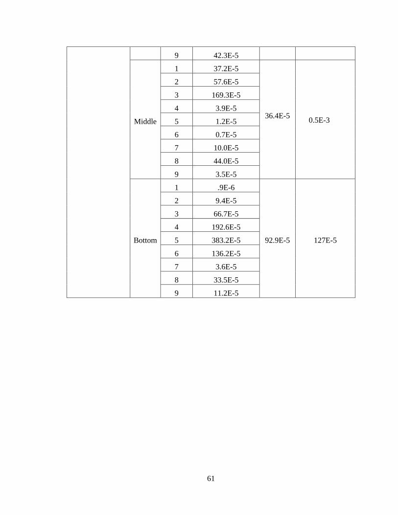
61
9 42.3E-5
Middle
1 37.2E-5
36.4E-5
0.5E-3
2 57.6E-5
3 169.3E-5
4 3.9E-5
5 1.2E-5
6 0.7E-5
7 10.0E-5
8 44.0E-5
9 3.5E-5
Bottom
1 .9E-6
92.9E-5 127E-5
2 9.4E-5
3 66.7E-5
4 192.6E-5
5 383.2E-5
6 136.2E-5
7 3.6E-5
8 33.5E-5
9 11.2E-5

62
Table 4.4 TSR calculation
TSR Calculation for AASHTO T 283 Conditioned Samples
Pavement
Section
Dry
Samples
ID
IDT
(psi)
Aver.
IDT
(psi)
T 283
samples
ID
IDT (psi) Ave.
IDT
(psi)
TSR Ave.
9 Top
layer
1 239.09 190.36 4 197.32 146.31 0.77 0.82
2 175.68 5 115.70
3 156.33 6 125.92
Middle
layer
1 189.31 189.23 4 141.41 132.66 0.7
2 185.44 5 138.20
3 193.93 6 118.39
Bottom
layer
1 81.16 91.25 4 142.58 92.84 1
2 101.33 5 48.04
3 79.18 6 87.90
TSR Calculation for MIST Conditioned Samples
Pavement
Section
Dry
Sample
s ID
IDT
(psi)
Average
IDT
(psi)
MIST
samples
ID
IDT
(psi)
Ave.
IDT
(psi)
TSR Ave.
9 Top
layer
1 239.09 190.36 7 157.57 168.64 0.89 0.87
2 175.68 8 166.31
3 156.33 9 182.03
Middle 1 189.31 189.23 7 109.01 135.12 0.71

63
layer 2 185.44 8 130.25
3 193.93 9 166.10
Bottom
layer
1 81.16 91.25 7 85.01 91.07 1
2 101.33 8 93.90
3 79.18 9 94.32

64
Good performing pavements
Bad performing pavements
Figure 4.1 Gradation curve for all pavement sections
12.5 9.5 4.75 2 0.425 0.075 0
10
20
30
40
50
60
70
80
90
100
Per
cen
t p
assi
ng
Sieve size raised to 0.45 power
(a) 12.5 mm NMAS
Max density line
US285MP126.3BL
US285MP140.53BL
US491MP60.9ML
US491MP60.9BL
19 12.5 9.5 4.75 2 0.425 0.075
0
10
20
30
40
50
60
70
80
90
100
Per
cen
t p
assi
ng
Sieve size raised to 0.45 power
(b) 19 mm NMAS
Max density line
US285MP126.3TL
US285MP140.53TL
US285MP285.25TL
US285MP285.25ML
US285MP285.25BL
US491MP60.9TL
US491MP60.5TL
US491MP60.5ML
US491MP60.5BL
US491MP60.7TL
US491MP60.7ML
US491MP60.7BL
NM14MP46.8TL
NM14MP46.8ML
NM14MP46.8BL
NM14MP46.9TL
NM14MP46.9ML
NM14MP46.9BL
12.5 9.5 4.75 2 0.425 0.075 0
10
20
30
40
50
60
70
80
90
100
Per
cen
t p
assi
ng
Sieve size raised to 0.45 power
(c) 12.5 mm NMAS
Max density line
US264MP10TL
112.5 9.5 4.75 2 0.425 0.075
0
10
20
30
40
50
60
70
80
90
100P
erce
nt
pas
sin
g
Sieve size raised to 0.45 power
(d) 19 mm NMAS
Max density line
US70MP289.26TL
US70MP289.26ML
US70MP289.26BL
US70MP282.2TL
US70MP282.2ML
US70MP282.2BL
US70MP272.67TL
US70MP272.67ML
US70MP272.67BL
NM344MP1.82TL
NM344MP1.8TL
NM344MP1.84
25

65
Figure 4.2 Field permeability at different damage conditions.
0
50
100
150
200
250
300
9 10 11 12 13 14 15 16
Per
mea
bil
ity (
x1
0-5
cm
/s)
(b) Bad performing pavements
Ave. k = 312×10-5
cm/s
k= 125×10-5 cm/s
0
50
100
150
200
250
300
1 2 3 4 5 6 7 8
Per
mea
bil
ity (
x1
0-5
cm
/s)
(a) Good performing pavement sections
Ave k = 62.7E-5
k = 125×10-5 cm/s
a

66
Figure 4.3 Laboratory full depth permeability at different damage conditions
0
10
20
30
40
50
60
70
80
90
100
1 2 3 4 5 6 7 8
Per
mea
bil
ity (
×1
0-5
cm
/s)
(a) Good performing sections
Ave. k =4.15×10⁻⁵cm/s 0
10
20
30
40
50
60
70
80
90
100
9 10 11 12 13 14 15
Per
mea
bil
ity (
×1
0-5
cm
/s)
(b) Bad performing sections
Ave. k = 69.7× 10⁻⁵ cm/s

67
Figure 4.4 Laboratory permeability of separated samples at different damage conditions
0
50
100
150
200
250
300
Top Layer Middle Layer Bottom Layer
Per
mea
bil
ity (
x1
0-5
cm
/s)
(b) Different layers of bad performing sections
9 10 11 12
13 14 15 16
Ave. k = 78.6 × 10⁻⁵ cm/s
k = 125 × 10-5 cm/s
0
50
100
150
200
250
300
Top Layer Middle Layer Bottom Layer
Per
mea
bil
ity (
×1
0-5
cm
/s)
(a) Different layers of good performing pavement section
1 2 3 4 5 6 7 8
Ave. k =22.9×10⁻⁵ cm/s
k = 125 × 10-5 cm/s

68
Figure 4.5 Correlation of MIST TSR and permeability at different modes.
R² = 0.0886
0
0.1
0.2
0.3
0.4
0.5
0.6
0.7
0.8
0.9
1
0 50 100 150 200 250 300 350
MIS
T T
SR
(c) Permeability of layered samples (×10-5 cm/s)
R² = 0.0166
0
0.1
0.2
0.3
0.4
0.5
0.6
0.7
0.8
0.9
1
0 100 200 300 400 500
MIS
T T
SR
(a) Field permeability (×10-5 cm/s)
R² = 0.0811
0
0.1
0.2
0.3
0.4
0.5
0.6
0.7
0.8
0.9
1
0 10 20 30
MIS
T T
SR
(b) Laboratory full depth k (×10-5 cm/s)
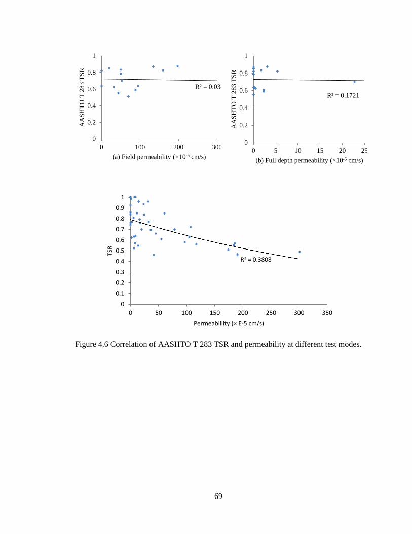
69
Figure 4.6 Correlation of AASHTO T 283 TSR and permeability at different test modes.
R² = 0.3808
0
0.1
0.2
0.3
0.4
0.5
0.6
0.7
0.8
0.9
1
0 50 100 150 200 250 300 350
TSR
Permeabillity (× E-5 cm/s)
R² = 0.0349
0
0.2
0.4
0.6
0.8
1
0 100 200 300
AA
SH
TO
T 2
83
TS
R
(a) Field permeability (×10-5 cm/s)
R² = 0.1721
0
0.2
0.4
0.6
0.8
1
0 5 10 15 20 25
AA
SH
TO
T 2
83
TS
R
(b) Full depth permeability (×10-5 cm/s)

70
Figure 4.7 Permeability at different test modes
0
50
100
150
200
250
1 2 3 4 5 6 7 15 9 10 11 12 13 14 14 16
Per
mea
bil
ity (
x1
0 -
5cm
/s)
Road sections
Field Permeability(cm/s) Lab k top layer (cm/s) Lab k full depth k (cm/s)

71
Figure 4.8 Comparisons between AASHTO T 283 and MIST TSR.
0
0.1
0.2
0.3
0.4
0.5
0.6
0.7
0.8
0.9
1
TS
R
Pavement Sections ( TL = Top layer, ML = Middle Layer, BL = Bottom Layer)
T 283 TSR MIST TSR

72
Figure 4.9 TSR values for good and bad performing pavement sections
0
0.1
0.2
0.3
0.4
0.5
0.6
0.7
0.8
0.9
1
Top layer Middle Layer Bottom layer
TS
R
Different layers
1
2
3
4
5
6
7
80.00
0.10
0.20
0.30
0.40
0.50
0.60
0.70
0.80
0.90
1.00
Top layer Middle layer Bottom layer
TS
R
Different layers
9
10
11
12
13
14
15
16
0
0.1
0.2
0.3
0.4
0.5
0.6
0.7
0.8
0.9
1
Top Layer Middle layer Bottom layer
TS
R
Different layers
1
2
3
4
5
6
7
8
0.00
0.10
0.20
0.30
0.40
0.50
0.60
0.70
0.80
0.90
1.00
Top layer Middle layer Bottom layer
TS
R
Different layers
9
10
11
12
13
14
15
16
(a) AASHTO T 283 TSR for good
performing sections
(b) AASHTO T 283 TSR for bad
sections
(c) MIST TSR for good pavement sections (d) MIST TSR for bad pavement sections

73
(a) Laboratory compacted samples
(b) Field cores
Figure 4.10 Permeability vs. air voids
0
10
20
30
40
50
60
70
80
90
100
0 2 4 6 8 10 12 14
Per
mea
bil
ity (
×1
0-5
cm
/s)
Air voids (%)
0
10
20
30
40
50
60
70
80
90
100
0 2 4 6 8 10 12 14
Per
mea
bil
ity (
x1
0-5
cm
/s)
Air voids (%)

74
(a) Permeability vs. TSR for laboratory compacted samples
(b) Comparision of AASHTO T 283 and MIST TSR for laboratory compacted samples
Figure 4.11 Permeability and moisture damage of labory compacted samples
R² = 0.0101
R² = 0.1089
0.00
0.20
0.40
0.60
0.80
1.00
1.20
0 5 10 15 20 25 30 35 40 45 50
TS
R
Permeability (x 10-5 cm/s )
0.00
0.20
0.40
0.60
0.80
1.00
1.20
1 2 3 4 5 6 7
TS
R
Axis Title
AASHTO T 283
MIST
SP III SP IV

75
CHAPTER 5
FIELD PERMEABILITY MODEL
5.1 INTRODUCTION
In this chapter, field permeability is determined by testing cored samples in the laboratory
by two proposed models. The models are then verified by laboratory and field
experiments. Initially, permeable pores of samples are determined in the laboratory using
a conventional tracer method. Field permeable pores are determined using laboratory
permeable pores and analytical method developed in this study. Finally, two models are
proposed to determine field permeability using field permeable porosity.
Component of a pore in AC: permeable pores, dead-end pores and isolated pores are also
measured correlated with the permeability and the moisture damage.
5.2 TRACER TEST
The laboratory setup for the tracer test is shown in Figure 5.1. Essentially, a salt
concentration-measuring meter was added to a falling head permeameter. Before placing
a sample in the laboratory permeameter, it was saturated using CorelokTM
device. The
sample was then placed inside a cylinder enclosed by a membrane and pressurized to
confine the side so that water flows in vertical direction only. Salt water of a known
concentration was poured inside the standpipe. The salt concentration of outflow was
measured using a salt concentration meter. Constant head was maintained by
continuously pouring water at inflow and discharge was measured. Darcy’s velocity is
determined using Eq. (5.1) and permeability is determined using Eq. (5.2):

76
(5.1)
(5.2)
where q = Darcy’s velocity, cm/s; Q = discharge rate, cm3/s; A = cross sectional area of
the sample, cm2; kl = laboratory permeability, L = length of the sample, cm; h = head,
cm. For the one-dimensional tracer, the outflow concentration was determined by Eq.
(5.3) (Stephen et al.1998):
(
) (5.3)
where erf = an error function; c = outflow salt concentration, %; c0 = inflow salt
concentration, %; v = mean velocity of the tracer, cm/s; D = dispersion coefficient, cm2/s;
and t = time, s. C/C0 = 0.5 occurred when one pore volume of solution passed through
the sample. The time required for C/C0 = 0.5 is known as break through time, tb.
Laboratory permeable pores (npl) can be calculated from Eq. (5.4) (Jury and Horton
2004):
(5.4)
Numerical Example 1:
For a core sample collected from New Mexico Highway 344 (NM344) (MP1.80), the
output from the salt concentration meter is shown in Figure 3.2. Salt concentration ratio
C/C0 is plotted against time. Ratio increases as time passes. Data is fitted to a sigmoidal
‘S’ shape curve. Breakthrough time from the graph can be found to be 58 s. The

77
measured Q is 0.645 cm3/s. Sample diameter, length and constant head are 14.2 cm, 8.1
cm, and 53.5 cm, respectively. Thus, plugging these values in Eq. (5.2) and Eq. (5.4):
61.8×10
-5 cm/s
and,
= 2.915%
5.3 FIELD PERMEABILITY MODEL
Total pores in an asphalt concrete sample can be divided in eight broad categories as
shown in Figure 5.3(a). They are: a = pores that continue from top to bottom, b = dead-
end pores at the top of the sample, c = pores that continue from top to side, d = pores that
continue from bottom to side, e = dead-end pores at the bottom, f = pores that continue
from side to side, g = dead-end pores at the side, and h = isolated pores.
When one-dimensional permeability test is performed on such sample (Figure 5.3(a)),
water flow occurs because of pores shown as “a”, that is, the pores that continue from
top to bottom of the sample. In the field, a fraction of “c” contributes to the flow through
lateral flow. Therefore, permeable pores responsible for flow in the field are:
(5.5)
where npf = field permeable pores.
Assuming a field core with radius r has some permeable pores (a and c) at the top surface
and they are distributed uniformly. If β = is the percent of curve surface pores that travel
to top. Then, pores (Al) that continue from the side to the top of the sample can be
determined using Eq. (5.6):

78
(5.6)
where L is the sample length. Therefore, pores responsible for vertical flow (Apl ) can be
determined by the following Eq. (5.7):
(5.7)
where α = percent of the surface top area occupied by c and a pores, πr2α = flow area
through c and a pores. In volumetric unit (dividing Eq. (5.7) by πr2), laboratory
permeable pores are:
(5.8)
where npl = laboratory permeable pores and γ = Lβ, a factor. Solving Eq. (5.8) for two
different sample sizes yields:
(5.9)
(5.10)
Hall and Ng (2001) have shown that the intensity of pores that continues from the side to
the top of the sample is not uniformly distributed on the side. The intensity is higher near
the top than the bottom. In this study, a triangular distribution of pore intensity may be
assumed on the side of the sample (Figure 5.3(b)). In addition, β-pores near the top of the
sample are less likely to continue to the bottom of the sample. In other words, β-pores
near the top have small contribution to permeability. Therefore, permeable pore intensity
can be assumed to be minimum (0.0) at the top and maximum (1.0) at the bottom. This
distribution is shown in Figure 5.3(b) schematically.

79
For a differential length dy as shown in Figure 5.3(b), lateral pores that continue from
side to top can be expressed as:
[
] (5.11)
Probability of these pores to continue to the bottom is:
(5.12)
Therefore, part of dAl that is permeable pores in case of field testing is:
[
]
(5.13)
Integration of Eq. (5.13) yields the total portion of the lateral pores that continues from
the top to the bottom and given below:
(5.14)
Therefore, the total permeable pores are (adding Eq. (5.7) with Eq. (5.14)):
(5.15)
In the volumetric unit:
(5.16)
where npf = field permeable pores, γ and r were defined previously.
Model 1:
Assuming permeability increases exponentially (with base e and permeable pores as
exponent), it can be written:
(5.17)

80
where m is a constant and np is permeable pores. m is determined by solving Eq. (5.17)
for two different sample sizes as follows:
(5.18)
where kl1 = laboratory measured permeability of 6 in. diameter sample, kl2 = laboratory
measured permeability of 4 in. diameter sample cored from the 6 in. diameter sample, npl1
= laboratory measured permeable pores of 6 in. diameter sample, and npl2 = laboratory
measured permeable pores of 4 in. diameter sample cored from the 6 in. diameter sample.
Finally, field permeability (kf) can be predicted using Eq. (5.19):
(5.19)
Model 2:
Assuming permeability varies exponentially (with permeable pores as base):
(5.20)
where µ is a constant and np was defined before. μ is determined by solving Eq. (5.20)
for two different sample sizes as follows:
(5.21)
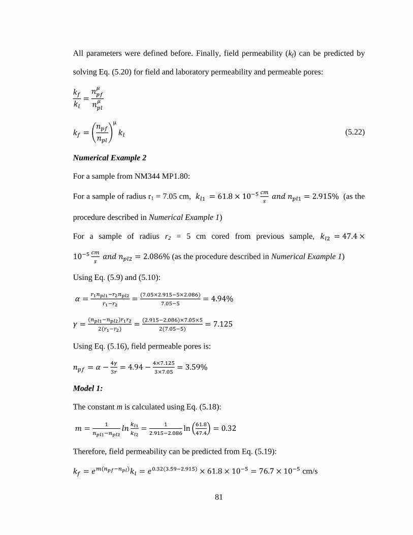
81
All parameters were defined before. Finally, field permeability (kf) can be predicted by
solving Eq. (5.20) for field and laboratory permeability and permeable pores:
(
)
(5.22)
Numerical Example 2
For a sample from NM344 MP1.80:
For a sample of radius r1 = 7.05 cm,
(as the
procedure described in Numerical Example 1)
For a sample of radius r2 = 5 cm cored from previous sample,
(as the procedure described in Numerical Example 1)
Using Eq. (5.9) and (5.10):
Using Eq. (5.16), field permeable pores is:
Model 1:
The constant m is calculated using Eq. (5.18):
(
)
Therefore, field permeability can be predicted from Eq. (5.19):
cm/s

82
Model 2:
The quantity μ can be calculated from Eq. (5.21):
Using Eq. (5.22):
(
)
(
)
cm/s
Tests on two more samples were performed and average permeability of three of the
samples was predicted as 391.5 cm/s which is much more than field permeability
determined on that location (69.7 cm/s). Laboratory permeability for this
location is 210.2 cm/s. Therefore, field permeability measurement gives
unsatisfactory and predicted permeability yields a satisfactory result. Detailed discussion
will be introduced in later section.
5.4 SELECTION OF CANDIDATE PAVEMENT
For moisture damage and permeability analysis, sixteen pavements were used. Among
them, nine pavement sections have high permeability. For tracer test, the sample needs to
be permeable. Therefore, the permeable nine pavement sections shown in Table 9 were
used for tracer test and further analysis.
5.5 RESULTS AND DISCUSSION
5.5.1 Different Pores and Their Correlation with Permeability
For each location, three samples were tested for permeable pores (npl) in the laboratory
using the tracer method. Average value of the three samples were determined and

83
correlated to effective pores (ne) and total pores (n). As shown in Figure 5.4(a), the solid
line represents the correlation between permeable pores and total pores and the dotted
line represents the correlation between permeable pores and effective pores. Overall, npl
doesn’t show good correlation with n, because total pores contain isolated and dead-end
pores. The relationship between npl and ne is pretty good as ne doesn’t include isolated
pores. The two regression lines are almost parallel as shown in Figure 35(a). That is, the
rate of increase of npl with total pore and effective pores are the same.
Figure 5.4(b) shows that there is a good linear relation between npl1 and npl2. The dotted
line in this figure indicates npl1 = npl2 (equal line). All points lay below the equal line
indicating npl1 > npl2. The regression line never intersects the equal line. This indicates
whatever value npl1 or np2 could have, they are not equal. These samples are identical but
have a different radius. It means their permeable pores vary in the radial direction.
Figure 5.5(a) shows correlation of permeability with total pores (n), effective pores (ne)
and permeable pores (np). Permeability shows very poor correlation with total pores as it
includes isolated and dead-end pores, which has no contribution to flow. Effective pores
show a better correlation with permeability. As permeability is directly controlled by
permeable pores, the correlation between permeability and permeable pores is pretty
good.
Figure 5.5(b) describes the correlation between laboratory permeability (kl) with
predicted field permeability (kf) (both of the models yield very close results, therefore
only model 1 is used for further discussion). This will reduce the efforts needed for
coring and measuring of np.

84
The measured permeable pore is less than effective pore and maintains a good correlation
with effective pore and permeability. Therefore it can be concluded that, the tracer
method gives a reasonable measurement of permeable pores of HMA.
5.5.2 Laboratory, Predicted and Field Measured Permeability
Figure 5.6 compares laboratory permeability, predicted permeability and field
permeability. Field tests on the first four sections were performed on the driving lane,
which was overlaid by an OGFC layer. Tests on the rest of the pavements were done on
the shoulders without having any OGFC. As expected, measured field permeability
results on the first four pavements are higher than the predicted permeability. For the
other five pavements, field permeability results are lower compared to the predicted
permeability. Measured field permeability values don’t show any regular relationship
with laboratory permeability, but predicted permeability does. Therefore, it can be stated
that the permeability estimation from the newly developed theory gives better prediction
of the field permeability of the compacted mix than.
To accommodate the field conditions (OGFC, coats etc.) a shift factor may be used with
predicted permeability to make it equal to measured permeability. For pavements with
OGFC, the ratio of measured to predicted permeability varies to a range of 4 to 22.
Therefore, measured and predicted permeability cannot be correlated in this case. For
pavements without OGFC, the ratio varies to a narrow range of 0.12 to 0.22 with an
average of 0.17. A regression analysis on predicted and measure value by Anova gives an
intercept of 9.43×10⁻⁵
cm/s with slope 0.132. The R2 value in this case 0.95 which is
pretty good. Finally, modified permeability is predicted using this regression analysis and

85
shown in Figure 5.6. The mean of error and standard deviation of error are 12.3% and
6.4% which are pretty good.
5.5.3 Quantification of Different Types of Pores and Their Relation with Moisture
Damage
Figure 5.7(a) compares isolated, permeable and dead-end pores of the nine pavement
sections. In all cases, permeable pores are higher than the other two types. Permeable
pores drain out water. Hence, it reduces the ‘moisture damage due to pumping action’.
On the other hand, dead-end pores hold the water for a long time after precipitation.
Therefore, it has greater impact on moisture damage due to the pumping action. Isolated
pores have no contribution on moisture or moisture related damage. Figure 5.7(b) shows
the correlation of TSR (indication of moisture damage) with permeable pores and dead-
end pores. As expected, moisture damage increases with the increase of dead-end pores
and decreases with the increase of permeable pores. In all cases, the MIST line is above
the AASHTO T 283 line, indicating less damage during MIST conditioning. The
correlations in Figure 5.7(b) are not good as other factors like binder grade, aggregate
type etc. was not considered during this study.
5.6 CONCLUSIONS
The following conclusions can be made from this study:
Combination of a permeameter with a salt meter can be used to determine
permeable pores of AC samples. Asphalt concrete sample’s permeability varies in
radial direction due to increase in permeable pore in radial direction. Tracer
method gives a reasonable measurement of permeable pores of AC samples.

86
Permeability shows a good relationship with permeable pores. The analytical
model developed in this study estimates field permeability of a HMA sample
tested in the laboratory reasonably well.
Pavement with more permeable pores is less susceptible to moisture damage.
Pavement with more dead-end pores is more susceptible to moisture damage.

87
Table 5.1 Pavement sections selected for tracer test
Pavement Sections Number of layer used (Top to bottom)
US285 MP140.53 1
US70 MP289.26 2
US70 MP 282.2 2
US70 MP272.67 2
US491 MP60.5 1
NM14 MP46.9 1
NM344 MP1.8 1
NM344 MP1.82 1
NM344 MP1.84 1

88
Figure 5.1 Permeable pores and permeability
set up.
Sample
Tube
Salt-meter

89
Figure 5.2 Breakthrough curve for a sample from NM344 at MP1.8.
0
0.1
0.2
0.3
0.4
0.5
0.6
0 5 10 15 20 25 30 35 40 45 50 55 60 65 70 75 80
Sal
t co
nce
ntr
atio
n r
atio
, C
/C0
Time (s)

90
(a) Pores distribution inside a cored sample (b) β (left triangle) and the probability
distribution (right triangle) on the side of
the sample.
Figure 5.3 Different types of pores in a sample.
dy
y
p
L-y
4πrβ
1
a b c
d e
f
g
h

91
(a) Correlation of permeable pores with total pores and effective pores
(b) Correlation between npl1 and npl2
Figure 5.4 Different types of pores and their correlation.
R² = 0.3804
R² = 0.6118
0
2
4
6
8
10
12
14
0 2 4 6 8 10 12 14 16
npl (
%)
n or ne (%)
npl vs. n
npl vs. ne
R² = 0.8299
0
2
4
6
8
10
12
14
0 2 4 6 8 10 12 14
npl2
(%
)
npl1 (%)

92
(a) Relation of permeability with n, ne, and npl
(b) Correlation between predicted and laboratory permeability
Figure 5.5 Different permeabilities and their relation with pores.
R² = 0.2298
R² = 0.5332
R² = 0.6677
0
500
1000
1500
2000
2500
3000
0 2 4 6 8 10 12 14
kl (
x1
0-5
cm
/s)
n, ne or npl
n vs. kl ne vs. kl npl vs. kl
y = 1.3294x + 21.831
R² = 0.9723
0
500
1000
1500
2000
2500
0 500 1000 1500 2000 2500
kf (x
10
-5 c
m/s
)
kl (x10-5 cm/s)
kf vs. kl

93
Figure 5.6 Comparison of field permeability with predicted and laboratory permeability.
0
100
200
300
400
500
600
700
800
900
1000
Per
mea
bil
ity (
×1
0-5
cm
/s)
Pavement sections
Laboratory k
Predicted k
Measured k
Modefied predicted k
Pavements with OGFC Pavements without OGFC
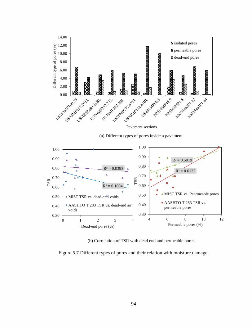
94
(a) Different types of pores inside a pavement
(b) Correlation of TSR with dead end and permeable pores
Figure 5.7 Different types of pores and their relation with moisture damage.
0.00
2.00
4.00
6.00
8.00
10.00
12.00
14.00
Dif
fere
nt
typ
e o
f p
ore
s (%
)
Pavement sections
isolated pores
permeable pores
dead-end pores
R² = 0.0393
R² = 0.1604
0.30
0.40
0.50
0.60
0.70
0.80
0.90
1.00
0 1 2 3 4
TS
R
Dead-end pores (%)
MIST TSR vs. dead-end voids
AASHTO T 283 TSR vs. dead-end air
voids
R² = 0.5019
R² = 0.6122
0.30
0.40
0.50
0.60
0.70
0.80
0.90
1.00
4 6 8 10 12
TS
R
Permeable pores (%)
MIST TSR vs. Pearmeable pores
AASHTO T 283 TSR vs.
permeable pores

95
CHAPTER 6
CONCLUSIONS AND RECOMMENDATIONS
6.1 SUMMARY
This study attempts to evaluate moisture damage and permeability characteristics of
asphalt pavements.
Moisture damage is evaluated in the field and in the laboratory. In the field, moisture
damage is initially identified by visual inspection of the pavements. Then visual
inspection of the stripping of the cores identifies the moisture damage condition of the
pavements more accurately and they are classified as good and bad performing
pavements in terms of moisture damage condition. Cores are brought to the laboratory
and TSR is determined by conventional the AASHTO T 283 and recently developed
MIST procedures. Cores collected from good performing pavements yield reasonably
higher TSR values than cores from the bad performing pavements, by both of the
methods. Although some good performing pavements have less TSR and some bad
performing pavements have more TSR value. Therefore none of the methods is very
close to the reality. MIST TSR values are almost always higher than the AASHTO T 283
TSR. The frost action of pore water in case of the AASHTO T 283 is responsible for that.
As more permeability represents more mix surface accessible to water, it can be stated
that permeability may influence moisture damage. To determine it, permeability of good
and bad performing pavements are determined and compared. It is obtained that, bad
performing pavements have higher permeability than good performing pavements.
Therefore, pavements with higher permeability are more susceptible to water. To

96
quantify the correlation between permeability and moisture damage, TSR values obtained
by the AASHTO T 283 and MIST are plotted against permeability. It is observed that
permeability doesn’t show any correlation with MIST TSR. The AASHTO T 283 TSR
shows a better correlation. As damage in the AASHTO T 283 is mainly governed by the
frost action of water, the more water a sample can hold, the more damage will occur. On
the other hand, damage in MIST occurs due to cyclic loading at elevated temperature. For
less permeable sample, it is still under cyclic loading elevated temperature and damage
occurs.
Permeability is determined both in field and in the laboratory. In the field, permeability is
determined on pavements with OGFC and without OGFC. In the laboratory, permeability
of full depth samples and samples separated in layers are determined. All this
permeability values are compared and it is tried to determine if there exists any
correlation between field and laboratory permeabilities. It is obtained that field
permeability cannot be correlated with laboratory permeability, as field permeability
depends on lot of factors. For pavements with OGFC, field permeability values are much
higher than laboratory permeability. Water may flow very quickly and laterally through
OGFC yielding higher permeability in the field. For pavements without OGFC, field
permeability values are much less than laboratory permeability of top layer. The
discontinuity of flow path and tack coat and seal coat may reduce the flow to a great
extent.
As field permeability may yield inaccurate results, it is necessary to determine it
alternatively. An analytical approach to determine field permeability by testing core in
the laboratory is introduced in this study. The first step of this method is to determine

97
permeable porosity using conventional tracer method. It is determined because
permeability depends only on permeable pores. Dead end and isolated pores have no
contribution to flow. Permeable pores are more in the field than in the laboratory because
in the laboratory specimen is confined at sides and there is no flow in the lateral
direction. Therefore, lateral permeable pores must be added to laboratory permeable
pores to determine field permeable pores. The analytical method introduced in this study
describes a procedure to determine field permeable pores. When field permeable pores
are known, field permeability can be determined using two models developed in this
study. Both models show very close results. The proposed models yield field
permeability more than laboratory permeability, which was expected. In case of
pavements with OGFC, the predicted permeability from model is less than the
permeability determined in the field. This is expected as field permeability tests on
OGFC overestimate the flow. In case of pavement without OGFC, the predicted
permeability from the models is more than the permeability determined in the field. It is
also expected as field permeameter underestimates the flow in this case. Therefore it can
be concluded that, the developed models yields reasonably well results. To accommodate
field boundary conditions like OGFC and different coats, a shift factor is proposed for
predicted permeability. Shift factor works very well for pavements without OGFC.
Almost all the previous studies focused on the permeability and total pores (air voids)
correlation, as it can be determined easily. As isolated or dead end pores have no
contribution to flow, the correlation is not realistic or feasible. This study correlates
permeability with permeable pores, which gives much better correlation than correlation
with total pores.

98
Total pores consist of the distinct type of pores: permeable pores, dead end pores and
isolated pores. This study determines these three types of pores. Permeable pores drain
out water quickly whereas dead end pores holds the water. Therefore these two quantities
may have correlation with moisture damage. This study shows that moisture damage
decrease with the increase of permeable pores and increase with the dead end pores. This
is expected because; permeable pores drain out water causing less interaction between
water and pavement. Dead end pores holds the water causing more damage due to
pumping action.
6.2 CONCLUSIONS
The following conclusions can be made from this study:
Both field and laboratory permeability of good performing sections are less than
the permeability of bad performing sections.
Cores from good performing sections have higher TSR values than cores from
bad performing section as determined by the AASHTO T 283 and MIST
procedures. The MIST TSR in most of the cases higher than the AASHTO T 283
TSR indicating less damage in MIST. For samples with very low air voids or
permeability, more damage occurs in the MIST than the AASHTO T 283.
Although MIST TSR doesn’t show any good correlation with permeability, the
AASHTO T 283 TSR shows a better correlation.
Permeability is better correlated with permeable porosity than total porosity and
effective porosity, as it eliminates dead end and isolated pores which have no
contribution to flow.
99
Moisture damage decreases with the increase of permeable pores and increases
with the increase of dead end pores.
A new analytical approach to determine field permeable pores as well as field
permeability by testing cores in the laboratory is developed in this study. The
model permeability is always greater than laboratory permeability as it includes
lateral flow. Pavement with and without OGFC overestimates and underestimates
permeability respectively. A shift factor of 0.132 with an intercept is applied to
match model permeability with field permeability for pavements without OGFC.
6.3 RECOMMENDATIONS
The following studies can be made further to establish this study:
• Hamburg wheel tracker may be used to determine the moisture susceptibility of
the mix. As it applies cyclic loading and wheel pressure similar to the field, this
prediction may be more useful and comparable with other test methods.
• A small single layer test pavement can be constructed over a highly permeable
sand layer with the facility of saturation. Field permeability test on that pavements
may give very accurate prediction, as there is no OGFC, tack coat, seal coat and
discontinuity of flow path. Laboratory permeability of the cores collected from
this pavement can be used to verify the model proposed in this study.

100
REFERENCES
AASHTO Standard T 283. Standard Method of Test for Resistance of Compacted Hot
Mix Asphalt (HMA) to Moisture-Induced Damage. AASHTO Guide,
Washington, DC, 2007.
Ahmad, M., and R. A. Tarefder. Addressing Permeability of SuperPave Mixes In New
Mexico. 3rd Quarter FY13, ORA 456-340, Research Bureau, New Mexico
Department of Transportation, 2013, pp. 1-43.
Al-Omari, A., L. Tashman, E. Masad, A. Cooley, T. Harman. 2002. “Proposed
Methodology for Predicting HMA Permeability.” J. Assoc. Asphalt Pav.
Technology, 71.
ASTM D 6752. Standard Test Method for Bulk Specific Gravity and Density of
Compacted Bituminous Mixtures Using Automatic Vacuum Sealing Method.
American Society for Testing and Materials, PA.
ASTM D 6857: Standard Test Method for Maximum Specific Gravity and Density of
Bituminous Paving Mixtures Using Automatic Vacuum Sealing Method.
Bear, J. Dynamics of Fluids in Porous Media. American Elsevier Publishing Company.
Inc., 1972.
Bhattacharjee, S., and R. B. Mallick. An Alternative Approach for the Determination of
Bulk Specific Gravity and Permeability of Hot Mix Asphalt (HMA). International
Journal of Pavement Engineering. Vol 3, No. 3, 2002, pp. 143-152.
Brown, E. R., M. R. Hainin, A. Cooley, and G. Hurley. Relationship of Air Voids, Lift
Thickness, and Permeability in Hot Mix Asphalt Pavements. NCHRP Report 531,
2004.

101
California Test 341: Method of Test for Measuring the Permeability of Bituminous
Pavements and Seal Coats.
Celik, O.N., (2005) “Air Permeability of Asphalt Concrete Made with Shredded-Tire
Rubber- Modified Binders and its Relationship with Porosity.”J. of Testing and
Evaluation, 33(4), 217–221.
Choubane, B., Page, G.C., and Musselman, J.A. (2007).“Effects of Water Saturation
Level on Resistance of Compacted Hot-Mix Asphalt Samples to Moisture-
Induced Damage.”In Trans. Res. Rec. J. of the Trans. Res. Board, 1723(2000),
TRB, National Research Council, Washington, D.C., 97–106.
Cooley, Jr., L. A., B. D. Prowell, and E. R. Brown. Issues Pertaining to the Permeability
Characteristics of Coarse Graded SuperPave Mixes. 2002 Annual Meeting of the
Association of Asphalt Paving Technologists.
Cooley Jr., L.A. 1999. “Permeability Of Superpave Mixtures: Evaluation of Field
Permeameters” NCAT Report No. 99-1.
FM 5-565: Florida Method of Test for Measurement of Water Permeability of Compacted
Asphalt Paving Mixtures.
Gogula, A. K., M. Hossain, and S. A. Romanoschi. A Study of Factors Affecting the
Permeability of Superpave Mixes in Kansas. Final report, Report No. K-TRAN:
KSU-00-2, 2004.
Hainin, M. R., L. A. Cooley, Jr., and B. D. Prowell. An Investigation of Factors
Influencing Permeability of Superpave Mixes. TRB 2003 Annual Meeting.
102
Hall, K. D., and H. G. Ng. Development of Void Pathway Test for Investigating Void
Interconnectivity in Compacted Hot-Mix Asphalt concrete. Journal of
Transportation Research Board, Volume 1767, 2001, pp. 40-47.
Harris, C.H. 2007. “Hot Mix Asphalt Permeability: Tester Size Effect and Anisotropy.”
MS thesis, Virginia Polytechnic Institute and State University.
Hicks, R. G. (1991). Moisture Damage in Asphalt Concrete: Synthesis of Highway
Practice, NCHRP Report 175.
InstroTek, Inc. Moisture Induced Sensitivity Test. Raleigh, NC, 2012.
Jones, S.C. 1997. “A Technique for Faster Pulse Decay Permeability Measurements in
Tight Rocks” SPE formation evaluation, SPE 28450.
Jury, W.A., and R. Horton. Soil Physics. 6th Edition, John Wiley and Sons, Inc., 2004.
Kanitpong, K., H. Bahia, J. Russell, and R. Schmitt. Predicting Field Permeability from
Testing Hot-Mix Asphalt Specimens Produced by Superpave Gyratory
Compactor. Journal of Transportation Research Board, No.1929, 2005, pp. 52-
58.
Kim, S., and Coree, B.J. (2005).Evaluation of Hot Mix Asphalt Moisture Sensitivity
Using the Nottingham Asphalt Test Equipment. IHRB Project TR-483.
Koponen, A., M. Kataja, and J. Timonen. Permeability and Effective Porosity of Porous
Media. The American Physical Society, Vol. 56, No. 3, 1997, pp. 3319-3325.
Liang, R.Y. (2008).Refine AASHTO T283 Resistance of Compacted Bituminous
Mixture to
Moisture Induced Damage for Superpave.Final Report FHWA/OH-2008-1.
103
Liang, Z., M. A. Ioannidis, and I. Chatzis. Permeability and Electrical Conductivity of
Porous Media from 3D Stochastic Replicas of the Microstructure. Chemical
Engineering Science, Vol. 55, Issue 2000, 2000, pp. 5247-5262.
Masad, E., Castelblanco, A., and Birgisson, B. (2006). “Effects of air void size
distribution, pore pressure, and bond energy on moisture damage.”J. of Testing
and Evaluation, 34(1), 15–23.
Masad, E., B. Birgisson, A. Al-Omari, and A. Cooley, 2002. “Analysis Of Permeability
And Fluid Flow In Asphalt Mixes” A Paper Submitted to the 82nd Annual
Transportation Research Board for Presentation and Publication.
Mallick, R. B., L. A. Cooley, Jr., M. R. Teto, R. L. Bradbury, and D. Peabody. An
Evaluation of Factors Affecting Permeability of Superpave Designed Pavements.
NCAT Report 03-02, 2003.
Menard, J., and J. A. Crovetti. Comparative Analysis of Field Permeability Testing of
Compacted Hot-Mix Asphalt Pavements. Journal of Transportation Research
Board, No.1946, 2006, pp. 147–156.
Mercado, E.A. (2007).Influence of fundamental material properties and air void structure
on moisture damage of asphalt mixes,” PhD Thesis submitted to Texas A&M
University.
Mogawer, W.S., Mallick, Teto, M.R., and Crockford, W.C. (2002). Evaluation of
Permeability of Superpave Mixes. NETCR 34, New England Transportation
Consortium, North Dartmouth, MA, Project No. NETC 00-2.
Mohammad, L. N., A. Herath, and B. Huang. Evaluation of Permeability of Suparpave
Paving Mixture. TRB 2003 Annual Meeting.

104
Ranieri, V., M. C. Antonnaci, G. Ying, and J. J. Sansalone. Application of Kozeny-
Kovàcs Model to Predict the Hydraulic Conductivity of Permeable Pavements.
Journal of Transportation Research Board, No. 2195, 2010, pp. 168-176.
Retzer, N.2008. “Permeability Research With the ROMUS Air Permeameter” Colorado
Department of Transportation, Final Report, Report No. CDOT-2008-5.
OHD L-44: Method Of Test For Measurement Of Water Permeability Of Compacted
Paving Mixtures.
Omari, A. A. Analysis of HMA Permeability through Microstructure Characterization
and Simulation of Fluid Flow in X-Ray CT Images. Dissertation submitted to
Texas A&M University, 2004.
Retzer, N. Permeability Research with the Romus Air Permeameter. Report to Colorado
DOT, Report No. CDOT-2008-5, 2008.
Rogowski, A. S. Flux Density and Breakthrough Times for Water and Tracer in A
Spatially Variable, Compacted Clay Soil. Journal of Contaminant Hydrology,
Vol.3, 1988, pp. 327-348.
Stephens, D. B., K. Hsu, M. A. Prieksat, M. D. Ankeny, N. Blandford, T. L. Roth, J. A.
Kelsey, and J. R. Whitworth. A Comparison of Estimated and Calculated
Effective Porosity. Hydrology Journal, Vol.6, 1998, pp. 156-165.
Tarefder, R. A., L. White, and M. Zaman. Neural Network Model for Asphalt Concrete
Permeability. Journal of Materials in Civil Engineering, Vol. 17, No. 1, 2005, pp.
19-27.
TEX 246-F: Test Procedure for Permeability or Water Flow of Hot Mix Asphalt.

105
Torres, A.C. (2004).Probabilistic Analysis of Air Void Structure and Its Relationship to
Permeability and Moisture Damage of Hot Mix Asphalt. MS Thesis submitted to
Texas A&M University.
Vivar, E., and J. E. Haddock. Hot Mix Asphalt Permeability and Porosity. Journal of the
Association of Asphalt Paving Technologist. Vol. 76, 2007, pp. 952-979.
Williams, S.G.2006. “A Comprehensive Study of Field Permeability Using the Vacuum
Permeameter.” MBTC-2054.
Willoughby, K. A., J. P. Mahoney, L. M. Pierce, J. S. Uhlmeyer, K. W. Anderson, S. A.
Read, S. T. Muench, T. R. Thompson and R. Moore 2001 “Construction-Related
Asphalt Concrete Pavement Temperature Differentials and the Corresponding
Density Differentials” Research report for Washington DOT.
Yeh, Y., C. Lee, and S. Chen. A Tracer Method to Determine Hydraulic Conductivity
and Effective Porosity of Saturated Clay under Low Gradient. Ground Water,
Vol.38, 2000, pp. 522-529.