Permanent Magnet Synchronous Drives Observability Analysis ... · Permanent Magnet Synchronous...
21
Permanent Magnet Synchronous Drives Observability Analysis for Motion-Sensorless Control Mohamad Koteich, Student Member, IEEE, Abdelmalek Maloum, Gilles Duc and Guillaume Sandou KEYWORDS Sensorless control, Synchronous motor, Induction Motor, AC machine. Abstract Motion-sensorless control techniques of electrical drives are attracting more attention in different industries. The local observability of sensorless permanent magnet synchronous drives is studied in this paper. A special interest is given to the standstill operation condition, where sensorless drives suffer of poor performance. Both, salient and non-salient machines are considered. The results are illustrated using numerical simulations. I. I NTRODUCTION Permanent Magnet (PM) Synchronous Machine (SM) has been widely used in many potential industrial applications [8] [14]. It is known for its high efficiency and power density. Mohamad Koteich is with Renault S.A.S. Technocentre, 78288 Guyancourt, France, and also with L2S - CentraleSup´ elec - CNRS - Paris-Sud University, 91192 Gif-sur-Yvette, France (e-mail: [email protected]). Abdelmalek Maloum is with Renault S.A.S. Technocentre, 78288 Guyancourt, France (e-mail: abdel- [email protected]). Gilles Duc and Guillaume Sandou are with L2S - CentraleSup´ elec - CNRS - Paris-Sud University, 91192 Gif-sur-Yvette, France (e-mail: [email protected]; [email protected]). arXiv:1601.06130v1 [math.CA] 9 Jan 2016
Transcript of Permanent Magnet Synchronous Drives Observability Analysis ... · Permanent Magnet Synchronous...
Permanent Magnet Synchronous Drives
Observability Analysis for Motion-Sensorless
ControlMohamad Koteich, Student Member, IEEE,
Abdelmalek Maloum, Gilles Duc and Guillaume Sandou
KEYWORDS
Sensorless control, Synchronous motor, Induction Motor, AC machine.
Abstract
Motion-sensorless control techniques of electrical drives are attracting more attention in different
industries. The local observability of sensorless permanent magnet synchronous drives is studied in this
paper. A special interest is given to the standstill operation condition, where sensorless drives suffer
of poor performance. Both, salient and non-salient machines are considered. The results are illustrated
using numerical simulations.
I. INTRODUCTION
Permanent Magnet (PM) Synchronous Machine (SM) has been widely used in many potential
industrial applications [8] [14]. It is known for its high efficiency and power density.
Mohamad Koteich is with Renault S.A.S. Technocentre, 78288 Guyancourt, France, and also with L2S - CentraleSupelec -
CNRS - Paris-Sud University, 91192 Gif-sur-Yvette, France (e-mail: [email protected]).
Abdelmalek Maloum is with Renault S.A.S. Technocentre, 78288 Guyancourt, France (e-mail: abdel-
Gilles Duc and Guillaume Sandou are with L2S - CentraleSupelec - CNRS - Paris-Sud University, 91192 Gif-sur-Yvette,
France (e-mail: [email protected]; [email protected]).
arX
iv:1
601.
0613
0v1
[m
ath.
CA
] 9
Jan
201
6

High performance control of the PMSM can be achieved using vector control [32] [16] [9]
[7], which relies on the two-reactance theory developed by Park [38] [39], where an accurate
knowledge of the rotor position is required.
For many reasons, mainly for cost reduction and reliability increase [37], mechanical sensorless
control of electrical drives has attracted the attention of researchers as well as many large
manufacturers [44] [25] [2] [20]; mechanical sensors are to be replaced by algorithms that
estimate the rotor speed and position, based on electrical sensors measurement.
One interesting sensorless technique is the observer-based one, which consists of sensing the
machine currents and voltages, and using them as inputs to a state observer [33] that estimates
the rotor angular speed and position. There exists a tremendous variety of observers for PMSM
in the literature [5]. Kalman filter [26] [11] [12] and sliding mode observers [46] [21] are
among the most widely used observer algorithms in PMSM sensorless drives [45]. Nevertheless,
other nonlinear observers [27] are also developed [42] [50] [36] [28]. Observer-based techniques
rely on the machine mathematical model. Hence, depending on the modeling approach, three
categories of these techniques can be distinguished:
• Electromechanical model-based observers [18] [42] [11] [50] [13] [49].
• Back electromotive force (EMF)-based observers [15] [35] [3] [24].
• Flux-based observers [36] [29] [10] [22] [30].
Another sensorless technique is the high frequency injection (HFI) based technique [17] [4]
[34]. Some authors propose to combine Observer-based and HFI techniques [1] [48] [31].
The main problem of the PMSM observer-based sensorless techniques is the deteriorated
performance in low- and zero-speed operation conditions [43]. This problem is usually treated
from observer’s stability point of view, whereas the real problem remains hidden: it lies in the
so-called observability conditions of the machine. Over the past few years, a promising approach,
based on the local weak observability concept [23], has been used in order to better understand
the deteriorated performance of sensorless drives.
Even though several papers have been published about the PMSM local observability, none of
these papers presents well elaborated results for both salient and non-salient PMSMs, especially
at standstill:
• Surface-mounted PMSM (SPMSM): in [50] and [19] the SPMSM observability is studied;
only the output first order derivatives are evaluated, and the conclusion is that the SPMSM

local observability cannot be guaranteed if the rotor speed is null. In [47] higher order
derivatives of the output are investigated, and it is shown that the SPMSM can be locally
observable at standstill if the rotor acceleration is nonzero.
• Internal PMSM (IPMSM): concerning the IPMSM, the conclusions in [47] are unclear,
i.e. no explicit practical observability conditions are given. More interesting results are
presented in [43], where explicit conditions, expressed in the rotating reference frame, are
presented. However, the analysis of the results in [43] remains unclear and yet inaccurate.
In [31], a unified approach is adopted for synchronous machines observability study; the
PMSM is treated as a special case of the generalized synchronous machine without further
analysis.
The present paper is intended to investigate the PMSM observability for the electromechanical
model-based observers. Both salient type (IPMSM) and non-salient type (SPMSM) machines
observability analysis is detailed. A special attention is drawn to the standstill operation condition.
After this introduction, the paper is organized as follows: the local weak observability theory is
presented in section II. Section III is dedicated to the PMSM’s mathematical model in both stator
and rotor reference frames. The observability analysis of the IPMSM is presented in section IV,
whereas the SPMSM observability is analyzed in section V. Illustrative simulations are presented
in section VI to validate the theoretical study. Conclusions are drawn in section VII.
II. LOCAL OBSERVABILITY THEORY
The local weak observability concept [23], based on the rank criterion, is presented in thissection. The systems of the following form (denoted Σ) are considered:
Σ :
x = f (x(t), u(t))
y = h (x(t))
(1)
where x ∈ X ⊂ Rn is the state vector, u ∈ U ⊂ Rm is the control vector (input), y ∈ Rp is
the output vector, f and h are C∞ functions. The observation problem can be then formulated
as follows [6]: Given a system described by a representation (1), find an accurate estimate x(t)
for x(t) from the knowledge of u(τ), y(τ) for 0 ≤ τ ≤ t.

A. Observability rank condition
The system Σ is said to satisfy the observability rank condition at x0 if the observabilitymatrix, denoted by Oy(x), is full rank at x0. Oy(x) is given by:
Oy(x) =∂
∂x
L0fh(x)
Lfh(x)
L2fh(x)
. . .
Ln−1f h(x)
T
x=x0
(2)
where Lkfh(x) is the kth-order Lie derivative of the function h with respect to the vector fieldf . It is given by:
Lfh(x) =∂h(x)
∂xf(x) (3)
Lkfh(x) = LfLk−1
f h(x) (4)
L0fh(x) = h(x) (5)
B. Observability theorem
A system Σ (1) satisfying the observability rank condition at x0 is locally weakly observable
at x0. More generally, a system Σ (1) satisfying the observability rank condition for any x0,
is locally weakly observable. Rank criterion gives only a sufficient condition for local weak
observability.
III. PMSM MATHEMATICAL MODEL
Permanent magnet synchronous machines are electromechanical systems that can be math-
ematically represented using generalized Ohm’s, Faraday’s, and Newton’s second Law. This
section presents the PMSM model in two reference frames: the stator reference frame αβ, and
the rotor reference frame dq [38] [39].
The assumption of linear lossless magnetic circuit is adopted, with sinusoidal distribution of
the stator magnetomotive force (MMF). The machine parameters are considered to be known
and constant. Nevertheless, the parameters variation does not call the observability study results
into question; it impacts the observer performance, which is beyond the scope of this study.

A. PMSM model in the stator reference frame
The mathematical model of the PMSM in the stator reference frame can be written as:dIdt
= L−1 (V −ReqI − ψrC ′(θ)ω)
dω
dt=p
J(Tm − Tl)
dθ
dt= ω
(6)
where I =[iα iβ
]Tand V =
[vα vβ
]Tstand for currents and voltages vectors in the αβ
reference frame, ω is the electrical speed of the rotor, θ is its electrical position, ψr is the rotor
permanent magnet flux. L is the inductance matrix, Req is the equivalent resistance matrix:
Req = R + ωL′ =
R 0
0 R
+ ω
∂L
∂θ(7)
R is the resistance of one stator winding. p is the number of pole pairs, J is the inertia of the
rotor with the load, Tl is the resistant torque, and Tm is the motor torque. C ′(θ) denotes the
partial derivative of C(θ) with respect to θ:
C(θ) =
cos θ
sin θ
; C ′(θ) =
∂C(θ)∂θ
=
− sin θ
cos θ
(8)
The model (6) can be fitted to the structure Σ (1) by taking:
x =[IT ω θ
]T; y = I ; u = V (9)
f(x, u) =[dITdt
dωdt
dθdt
]T; h(x) = I (10)
1) IPMSM: The IPMSM is a salient rotor machine, then its inductance matrix L is a position-
dependent matrix:
L =
L0 + L2 cos 2θ L2 sin 2θ
L2 sin 2θ L0 − L2 cos 2θ
(11)
where L0 and L2 are the average and differential spatial inductances. The IPMSM produced
torque is:
Tm =3p
2[ψr(iβ cos θ − iα sin θ) (12)
−L2
((i2α − i2β) sin 2θ − 2iαiβ cos 2θ
)]

vα
vβ
d
q
θ
α
β
(a) IPMSM
vd
vq
d
q
θ
α
β
(b) SPMSM
Fig. 1: Schematic representation of IPMSM and SPMSM
2) SPMSM: The SPMSM is a non-salient rotor machine, its model can be derived from the
IPMSM one by assuming L2 to be null:
L2 = 0 (13)
B. PMSM model in the rotor reference frame
Stator currents and voltages in the dq rotating reference frame (Fig. 1) are calculated from
those in the αβ reference frame using the Park transform:
Xdq = P−1(θ)Xαβ (14)
where
P(θ) =
cos θ − sin θ
sin θ cos θ
(15)
The vector X stands for currents or voltages vector. The mathematical model of the PMSM in
the rotor reference frame can be then written under the general form (6):
dIdqdt
= L−1dq
(Vdq −Req
dqIdq − ψrC′(0)ω
)
dω
dt=p
J(Tm − Tl)
dθ
dt= ω
(16)

where Idq =[id iq
]Tand Vdq =
[vd vq
]Tstand for currents and voltages vectors in the dq
reference frame. Inductance and equivalent resistance matrices can be written as:
Ldq =
Ld 0
0 Lq
; Req
dq = R + ωJ2Ldq (17)
where
J2 = P(π
2
)=
0 −1
1 0
(18)
Ld denotes the (direct) d−axis inductance, and Lq denotes the (quadrature) q−axis inductance:
Ld = L0 + L2 (19)
Lq = L0 − L2 (20)
The motor torque can be written as:
Tm =3
2p (Lδid + ψr) iq (21)
with
Lδ = Ld − Lq = 2L2 (22)
The above dq model is valid for the IPMSM (Ld 6= Lq). The SPMSM model can be derived
using the following equations:
Ld = Lq = L0 =⇒ Lδ = 0 (23)
IV. IPMSM OBSERVABILITY
Observability of the system (6) is studied in the sequel. The system (6) is a 4th order system.
Its observability matrix should contain the gradient of the output and its derivatives up to the
3rd order. In this section, only the first order derivatives are calculated, higher order derivatives
are very difficult to evaluate and to deal with. The “partial” observability matrix is:
Oy1 =∂(y, y)
∂x=
I2 O2×1 O2×1
∂∂I
(dIdt
)∂∂ω
(dIdt
)∂∂θ
(dIdt
)
(24)

where In is the n× n identity matrix, and On×m is an n×m zero matrix, and:
∂
∂I
(dIdt
)= −L−1Req
∂
∂ω
(dIdt
)= −L−1 (L′I + ψrC ′(θ)) (25)
∂
∂θ
(dIdt
)= (L−1)′L
dIdt− L−1 (L′′I − ψrC(θ))ω
L′ and L′′ denote, respectively, the first and second partial derivatives of L with respect to θ:
L′ =∂
∂θL ; L′′ =
∂
∂θL′ (26)
The determinant ∆y1 of the sub-matrix (24) is calculated using symbolic math software. In order
to make the interpretation easier, the determinant is expressed in the rotating dq reference frame
using the equation (14).
The determinant ∆y1 is given by:
∆y1 =1
LdLq
[(Lδid + ψr)
2 + L2δi
2q
]ω
+LδLdLq
[Lδdiddtiq − (Lδid + ψr)
diqdt
](27)
The observability condition ∆y1 6= 0 can be written as:
ω 6=(Lδid + ψr)Lδ
diqdt− Lδ diddt Lδiq
(Lδid + ψr)2 + L2
δi2q
(28)
which gives:
ω 6= d
dtarctan
(Lδiq
Lδid + ψr
)(29)
The equation (29) defines a fictitious observability vector, denoted by ΨO, that has the
following components in the dq reference frame:
ΨOd = Lδid + ψr (30)
ΨOq = Lδiq (31)
Then, the condition (29) can be formulated as:
ω 6= d
dtθO (32)
where θO is the phase of the vector ΨO in the rotating reference frame (Fig. 2). The following
sufficient condition for the PMSM local observability can be stated: the rotational speed of the
α
β
ΨO
θO
d
q
ψr
Lδid
Lδiq
θ
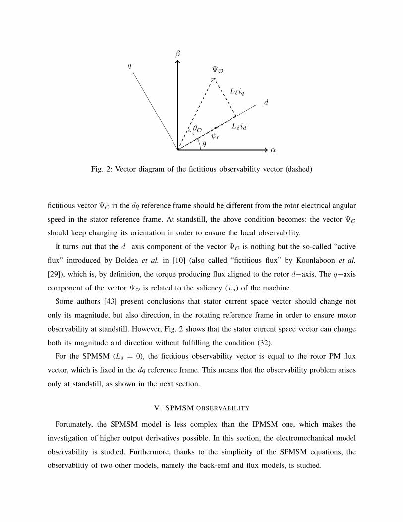
Fig. 2: Vector diagram of the fictitious observability vector (dashed)
fictitious vector ΨO in the dq reference frame should be different from the rotor electrical angular
speed in the stator reference frame. At standstill, the above condition becomes: the vector ΨO
should keep changing its orientation in order to ensure the local observability.
It turns out that the d−axis component of the vector ΨO is nothing but the so-called “active
flux” introduced by Boldea et al. in [10] (also called “fictitious flux” by Koonlaboon et al.
[29]), which is, by definition, the torque producing flux aligned to the rotor d−axis. The q−axis
component of the vector ΨO is related to the saliency (Lδ) of the machine.
Some authors [43] present conclusions that stator current space vector should change not
only its magnitude, but also direction, in the rotating reference frame in order to ensure motor
observability at standstill. However, Fig. 2 shows that the stator current space vector can change
both its magnitude and direction without fulfilling the condition (32).
For the SPMSM (Lδ = 0), the fictitious observability vector is equal to the rotor PM flux
vector, which is fixed in the dq reference frame. This means that the observability problem arises
only at standstill, as shown in the next section.
V. SPMSM OBSERVABILITY
Fortunately, the SPMSM model is less complex than the IPMSM one, which makes the
investigation of higher output derivatives possible. In this section, the electromechanical model
observability is studied. Furthermore, thanks to the simplicity of the SPMSM equations, the
observabiltiy of two other models, namely the back-emf and flux models, is studied.

A. Electromechanical model observability
In the case of SPMSM, the observability matrix Oy can be evaluated up to the 3rd order output
derivatives. Oy is an 8× 4 matrix. There are 70 possible 4× 4 sub-matrices. For convenience,
the first two lines are always taken, together with lines that correspond to the same derivation
order. This reduces the choices to the following 3 possible sub-matrices:
• Oy1, which includes the first 4 lines of Oy:
Oy1 =
1 0 0 0
0 1 0 0
− RL0
0 ψrL0
sin θ ω ψrL0
cos θ
0 − RL0−ψrL0
cos θ ω ψrL0
sin θ
(33)
its determinant is
∆y1 = ω
(ψrL0
)2
(34)
Thus, the local observability is guaranteed if the rotor speed is nonzero, but not in the case
of zero speed.
• Oy2, which includes the 1st, 2nd, 5th and 6th lines of Oy, its determinant is :
∆y2 =ψ2r
L20
[(2ω2 +
R2
L20
+3p2
Jψrid
)ω − R
L0
dω
dt
](35)
Thus, in the case of zero speed operation, the SPMSM is observable if the acceleration
is different than zero (ω 6= 0); this corresponds to the case where the motor changes its
rotation direction.
• Oy3, which includes the 1st, 2nd, 7th and 8th lines of Oy. Its determinant ∆y3 cannot be
written because it is lengthy. Nevertheless, substituting the rank deficiency conditions of
the sub-matrix Oy2 (ω = 0 and ω = 0) in ∆y3, under the assumption of very slow resistant
torque variation (Tl = 0), gives:
∆y3|∆y2=0 =ψ2r
L20
[R2
L20
− 3p2
2J(L0id + ψr)
ψrL0
]d2ω
dt2(36)
where
d2ω
dt2=
3p2
2Jψrdiqdt
(37)

If the speed is identically zero (ω ≡ 0), the SPMSM model reduces to:
dIdt
=1
L0
(V −RI)
dω
dt= 0 (38)
dθ
dt= 0
and the output derivatives are:
dIdt
=1
L0
(V −RI) (39)
d2Idt2
=1
L0
(dVdt−RdI
dt
)(40)
...dn+1Idtn+1
=1
L0
(dnVdtn−Rd
nIdtn
)(41)
In this case, the observability matrix is:
Oy|ω≡0 =
1 0 0 0
0 1 0 0
− RL0
0 ψrL0
sin θ 0
0 − RL0
−ψrL0
cos θ 0
(− RL0
)2 0 − RL0
ψrL0
sin θ 0
0 (− RL0
)2 RL0
ψrL0
cos θ 0
(− RL0
)3 0 (− RL0
)2 ψrL0
sin θ 0
0 (− RL0
)3 −(− RL0
)2 ψrL0
cos θ 0
(42)
The following recurrence can be obtained from (39)-(42) for higher dimension observability
matrices:
∂
∂xLkfh = − R
L0
∂
∂xLk−1f h|ω≡0 (43)
Therefore, even if higher order derivatives are evaluated, no additional information about the
rotor position can be extracted. Hence, the standstill operation condition presents a singularity
from observability viewpoint.
Physically speaking, if the non-salient (cylindrical) rotor is fixed with respect to the stator
windings, it will have no effect on the electromagnetic behaviour of these windings, and its
position cannot be identified with the model (38).

α
β
d
q
d
q
θθ
θ
Fig. 3: Vector diagram of stator (thick), estimated (dashed) and real rotor reference frames
One solution of this problem is proposed in [1]. It combines HFI technique with a state
observer algorithm; a sinusoidal voltage is injected on the direct (d−) axis in the estimated
rotating reference frame (Fig. 3), which results in a vibration of the rotor (nonzero speed) only
if the position is not correctly estimated. It is proved in [1] that if the following HF voltage
vd = Vhf cos(ωhf t) (44)
is injected in the estimated dq rotating reference frame (obtained by the Park transformation
using the estimated position θ), the determinant ∆y1 (34) becomes:
∆y1 = −ψ2r
L20
ω +ψrL2
0
Vhf cos(ωhf t) sin θ (45)
where θ stands for the position estimation error. If the position is not correctly estimated (θ 6= 0),
the local observability is guaranteed at standstill.
Another solution is proposed in [40] [41]. It consists of adding a position-dependent source,
g(θ), to the available measurements. The origin of g(θ) is found in the stator iron local B-
H hysteresis loops. It is shown that this signal is highly position-dependent, and it can be
approximated by a linear function:
g(θ) = aθ + b (46)
where a and b are two constants. The new output vector becomes:
y =[iα iβ aθ + b
]T(47)
Therefore, even at standstill, the position is observable.
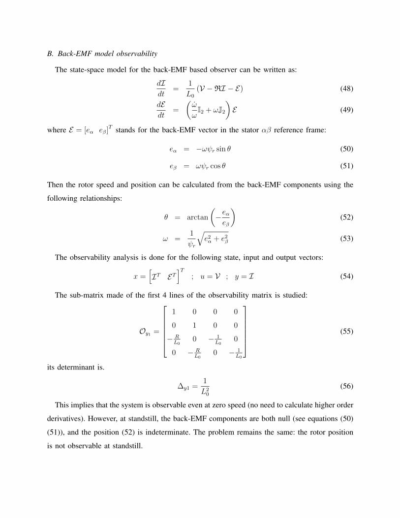
B. Back-EMF model observability
The state-space model for the back-EMF based observer can be written as:
dIdt
=1
L0
(V −RI − E) (48)
dEdt
=
(ω
ωI2 + ωJ2
)E (49)
where E = [eα eβ]T stands for the back-EMF vector in the stator αβ reference frame:
eα = −ωψr sin θ (50)
eβ = ωψr cos θ (51)
Then the rotor speed and position can be calculated from the back-EMF components using the
following relationships:
θ = arctan
(−eαeβ
)(52)
ω =1
ψr
√e2α + e2
β (53)
The observability analysis is done for the following state, input and output vectors:
x =[IT ET
]T; u = V ; y = I (54)
The sub-matrix made of the first 4 lines of the observability matrix is studied:
Oy1 =
1 0 0 0
0 1 0 0
− RL0
0 − 1L0
0
0 − RL0
0 − 1L0
(55)
its determinant is.
∆y1 =1
L20
(56)
This implies that the system is observable even at zero speed (no need to calculate higher order
derivatives). However, at standstill, the back-EMF components are both null (see equations (50)
(51)), and the position (52) is indeterminate. The problem remains the same: the rotor position
is not observable at standstill.
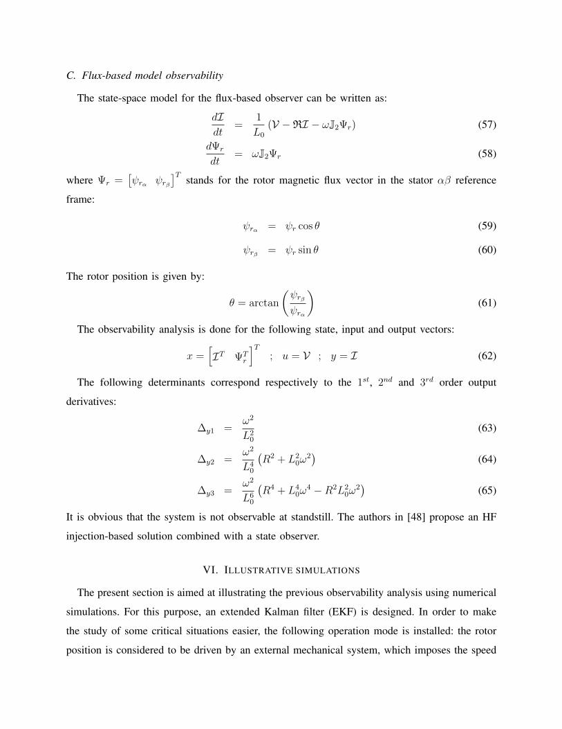
C. Flux-based model observability
The state-space model for the flux-based observer can be written as:
dIdt
=1
L0
(V −RI − ωJ2Ψr) (57)
dΨr
dt= ωJ2Ψr (58)
where Ψr =[ψrα ψrβ
]T stands for the rotor magnetic flux vector in the stator αβ reference
frame:
ψrα = ψr cos θ (59)
ψrβ = ψr sin θ (60)
The rotor position is given by:
θ = arctan
(ψrβψrα
)(61)
The observability analysis is done for the following state, input and output vectors:
x =[IT ΨT
r
]T; u = V ; y = I (62)
The following determinants correspond respectively to the 1st, 2nd and 3rd order output
derivatives:
∆y1 =ω2
L20
(63)
∆y2 =ω2
L40
(R2 + L2
0ω2)
(64)
∆y3 =ω2
L60
(R4 + L4
0ω4 −R2L2
0ω2)
(65)
It is obvious that the system is not observable at standstill. The authors in [48] propose an HF
injection-based solution combined with a state observer.
VI. ILLUSTRATIVE SIMULATIONS
The present section is aimed at illustrating the previous observability analysis using numerical
simulations. For this purpose, an extended Kalman filter (EKF) is designed. In order to make
the study of some critical situations easier, the following operation mode is installed: the rotor
position is considered to be driven by an external mechanical system, which imposes the speed

TABLE I: IPMSM Parameters
Parameters Value [Unit]
Number of pole pairs (p) 2
Stator resistance Rs 0.01 [Ω]
Direct inductance Ld 0.5 [mH]
Quadratic inductance Lq 0.8 [mH]
Rotor magnetic flux ψr 0.0225 [V.s/rad]
0 0.2 0.4 0.6 0.8 10
200
400
time(sec)
spee
d (r
ad/s
ec)
Fig. 4: Rotor speed profile
profile shown in Fig. 4. The currents are regulated, using standard proportional-integral (PI)
controllers, to fit with the following set-points:
i∗d = 0 A ; i∗q = 15 A (66)
Both IPMSM and SPMSM are studied in the same simulation environment. The same machine
parameters are used for both machines; the only difference is in the inductance L2, which is
null in the case of SPMSM (no saliency). The following HF current is added to the current iq
during the time interval [0.2 s., 0.5 s.]:
iqHF = 0.5 sin 1000πt A (67)
The purpose is to compare the observer behaviour for both machines at standstill, with and
without signal injection. The observer is operating in open-loop, the real position is fed to
the controller in order to avoid stability issues in the observability analysis. Table I shows the
machine parameters.
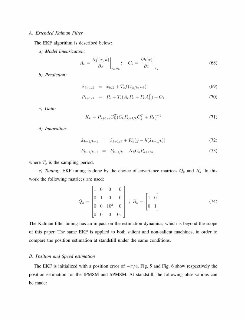
A. Extended Kalman Filter
The EKF algorithm is described below:
a) Model linearization:
Ak =∂f(x, u)
∂x
∣∣∣∣xk,uk
; Ck =∂h(x)
∂x
∣∣∣∣xk
(68)
b) Prediction:
xk+1/k = xk/k + Tsf(xk/k, uk) (69)
Pk+1/k = Pk + Ts(AkPk + PkATk ) +Qk (70)
c) Gain:
Kk = Pk+1/kCTk (CkPk+1/kC
Tk +Rk)
−1 (71)
d) Innovation:
xk+1/k+1 = xk+1/k +Kk(y − h(xk+1/k)) (72)
Pk+1/k+1 = Pk+1/k −KkCkPk+1/k (73)
where Ts is the sampling period.
e) Tuning: EKF tuning is done by the choice of covariance matrices Qk and Rk. In this
work the following matrices are used:
Qk =
1 0 0 0
0 1 0 0
0 0 103 0
0 0 0 0.1
; Rk =
1 0
0 1
(74)
The Kalman filter tuning has an impact on the estimation dynamics, which is beyond the scope
of this paper. The same EKF is applied to both salient and non-salient machines, in order to
compare the position estimation at standstill under the same conditions.
B. Position and Speed estimation
The EKF is initialized with a position error of −π/4. Fig. 5 and Fig. 6 show respectively the
position estimation for the IPMSM and SPMSM. At standstill, the following observations can
be made:

0 0.2 0.4 0.6 0.8 1−3
−2
−1
0
1
2
3
time(sec)
posi
tion(
rad)
rotor positionestimated position
Fig. 5: Rotor real and estimated position of the IPMSM
• Before injecting the HF current, the position estimation of the IPMSM is more accurate
than the SPMSM one.
• After injecting the HF current, the IPMSM estimated position converges to the real position,
whereas the SPMSM one slightly varies.
• The SPMSM estimated position converges to the real position value as soon as the rotor
accelerates.
These results are consistent with the observability study results; the IPMSM can be observable
at standstill, whereas observability of the SPMSM cannot be guaranteed unless the rotor moves.
The speed estimation error is shown in Fig. 7, it is almost the same for both machines.
VII. CONCLUSIONS
The local observability study of the PMSM resulted in the definition of a fictitious observability
vector; the rotational speed of this observability vector in the rotor reference frame should be
different from the rotor electrical speed in the stator reference frame to ensure the machine
observability.
The results presented in this paper are valid for a wide range of brushless synchronous ma-
chines under the assumption of sinusoidal stator MMF distribution: PM synchronous, Brushless
DC, PM stepper and PM assisted reluctance machines. Furthermore, if the rotor PM flux is
considered to be zero, the results can be extended to synchonous reluctance machines.

0 0.2 0.4 0.6 0.8 1−3
−2
−1
0
1
2
3
time(sec)
posi
tion(
rad)
rotor positionestimated position
Fig. 6: Rotor real and estimated position of the SPMSM
0 0.2 0.4 0.6 0.8 1−1
0
1
2
time(sec)
spee
d (r
ad/s
ec)
IPMSMSPMSM
Fig. 7: Rotor speed estimation error
REFERENCES
[1] F. Abry, A. Zgorski, Xuefang Lin-Shi, and J.-M. Retif. Sensorless position control for spmsm at zero speed and acceleration.
In Power Electronics and Applications (EPE 2011), Proceedings of the 2011-14th European Conference on, pages 1–9,
Aug 2011.
[2] P.P. Acarnley and J.F. Watson. Review of position-sensorless operation of brushless permanent-magnet machines. Industrial
Electronics, IEEE Transactions on, 53(2):352–362, April 2006.
[3] A. Akrad, M. Hilairet, and D. Diallo. Design of a fault-tolerant controller based on observers for a pmsm drive. Industrial
Electronics, IEEE Transactions on, 58(4):1416–1427, April 2011.
[4] A. Arias, C.A. Silva, G.M. Asher, J.C. Clare, and P.W. Wheeler. Use of a matrix converter to enhance the sensorless control
of a surface-mount permanent-magnet ac motor at zero and low frequency. Industrial Electronics, IEEE Transactions on,
53(2):440–449, April 2006.

[5] O. Benjak and D. Gerling. Review of position estimation methods for ipmsm drives without a position sensor part ii:
Adaptive methods. In Electrical Machines (ICEM), 2010 XIX International Conference on, pages 1–6, Sept 2010.
[6] Gildas Besancon. Nonlinear observers and applications. Lecture Notes in Control and Information Sciences. Springer,
Verlag/Heidelberg, New-York/Berlin, 2007.
[7] F. Betin, G.-A Capolino, D. Casadei, B. Kawkabani, R.I Bojoi, L. Harnefors, E. Levi, L. Parsa, and B. Fahimi. Trends in
electrical machines control: Samples for classical, sensorless, and fault-tolerant techniques. Industrial Electronics Magazine,
IEEE, 8(2):43–55, June 2014.
[8] B. Bilgin and A. Emadi. Electric motors in electrified transportation: A step toward achieving a sustainable and highly
efficient transportation system. Power Electronics Magazine, IEEE, 1(2):10–17, June 2014.
[9] I. Boldea. Control issues in adjustable speed drives. Industrial Electronics Magazine, IEEE, 2(3):32–50, Sept 2008.
[10] I. Boldea, M.C. Paicu, and G. Andreescu. Active flux concept for motion-sensorless unified ac drives. Power Electronics,
IEEE Transactions on, 23(5):2612–2618, Sept 2008.
[11] S. Bolognani, R. Oboe, and M. Zigliotto. Sensorless full-digital pmsm drive with ekf estimation of speed and rotor position.
Industrial Electronics, IEEE Transactions on, 46(1):184–191, Feb 1999.
[12] S. Bolognani, L. Tubiana, and M. Zigliotto. Extended kalman filter tuning in sensorless pmsm drives. Industry Applications,
IEEE Transactions on, 39(6):1741–1747, Nov 2003.
[13] M. Boussak. Implementation and experimental investigation of sensorless speed control with initial rotor position estimation
for interior permanent magnet synchronous motor drive. Power Electronics, IEEE Transactions on, 20(6):1413–1422, Nov
2005.
[14] A.K. Chattopadhyay. Alternating current drives in the steel industry. Industrial Electronics Magazine, IEEE, 4(4):30–42,
Dec 2010.
[15] Zhiqian Chen, M. Tomita, S. Doki, and S. Okuma. An extended electromotive force model for sensorless control of interior
permanent-magnet synchronous motors. Industrial Electronics, IEEE Transactions on, 50(2):288–295, Apr 2003.
[16] John Chiasson. Modeling and high performance control of electric machines, volume 26. John Wiley & Sons, 2005.
[17] M.J. Corley and R.D. Lorenz. Rotor position and velocity estimation for a salient-pole permanent magnet synchronous
machine at standstill and high speeds. Industry Applications, IEEE Transactions on, 34(4):784–789, Jul 1998.
[18] R. Dhaouadi, N. Mohan, and L. Norum. Design and implementation of an extended kalman filter for the state estimation
of a permanent magnet synchronous motor. Power Electronics, IEEE Transactions on, 6(3):491–497, Jul 1991.
[19] M. Ezzat, J. de Leon, N. Gonzalez, and A. Glumineau. Observer-controller scheme using high order sliding mode techniques
for sensorless speed control of permanent magnet synchronous motor. In Decision and Control (CDC), 2010 49th IEEE
Conference on, pages 4012–4017, Dec 2010.
[20] J.W. Finch and D. Giaouris. Controlled ac electrical drives. Industrial Electronics, IEEE Transactions on, 55(2):481–491,
Feb 2008.
[21] G. Foo and M.F. Rahman. Sensorless sliding-mode mtpa control of an ipm synchronous motor drive using a sliding-mode
observer and hf signal injection. Industrial Electronics, IEEE Transactions on, 57(4):1270–1278, April 2010.
[22] G.H.B. Foo and M.F. Rahman. Direct torque control of an ipm-synchronous motor drive at very low speed using a
sliding-mode stator flux observer. Power Electronics, IEEE Transactions on, 25(4):933–942, April 2010.
[23] R. Hermann and Arthur J. Krener. Nonlinear controllability and observability. Automatic Control, IEEE Transactions on,
22(5):728–740, Oct 1977.
[24] A. Hijazi, Xuefang Lin Shi, A. Zgorski, and L. Sidhom. Adaptive sliding mode observer-differentiator for position and

speed estimation of permanet magnet synchronous motor. In Sensorless Control for Electrical Drives (SLED), 2012 IEEE
Symposium on, pages 1–5, Sept 2012.
[25] J. Holtz. Sensorless control of induction machines - with or without signal injection? Industrial Electronics, IEEE
Transactions on, 53(1):7–30, Feb 2005.
[26] Rudolph Kalman. A new approach to linear filtering and prediction problems. Transaction of the ASME - Journal of Basic
Engineering, 82:35–45, 1960.
[27] H.K. Khalil. Nonlinear Control. Global. Pearson Education, London, 2015.
[28] A. Khlaief, M. Bendjedia, M. Boussak, and M. Gossa. A nonlinear observer for high-performance sensorless speed control
of ipmsm drive. Power Electronics, IEEE Transactions on, 27(6):3028–3040, June 2012.
[29] S. Koonlaboon and S. Sangwongwanich. Sensorless control of interior permanent-magnet synchronous motors based on
a fictitious permanent-magnet flux model. In Industry Applications Conference, 2005. Fourtieth IAS Annual Meeting.
Conference Record of the 2005, volume 1, pages 311–318 Vol. 1, Oct 2005.
[30] M. Koteich, T. Le Moing, A. Janot, and F. Defay. A real-time observer for uav’s brushless motors. In Electronics, Control,
Measurement, Signals and their application to Mechatronics (ECMSM), 2013 IEEE 11th International Workshop of, pages
1–5, June 2013.
[31] M. Koteich, A. Maloum, G. Duc, and G. Sandou. Observability analysis of sensorless synchronous machine drives. In
Control Conference (ECC), 2015 European, July 2015.
[32] W. Leonhard. Control of Electrical Drives. Engineering online library. Springer Berlin Heidelberg, 2001.
[33] D.G. Luenberger. An introduction to observers. Automatic Control, IEEE Transactions on, 16(6):596–602, Dec 1971.
[34] S. Medjmadj, D. Diallo, M. Mostefai, C. Delpha, and A. Arias. Pmsm drive position estimation: Contribution to the
high-frequency injection voltage selection issue. Energy Conversion, IEEE Transactions on, 30(1):349–358, March 2015.
[35] B. Nahid-Mobarakeh, F. Meibody-Tabar, and F.-M. Sargos. Mechanical sensorless control of pmsm with online estimation
of stator resistance. Industry Applications, IEEE Transactions on, 40(2):457–471, March 2004.
[36] R. Ortega, L. Praly, A. Astolfi, Junggi Lee, and Kwanghee Nam. Estimation of rotor position and speed of permanent
magnet synchronous motors with guaranteed stability. Control Systems Technology, IEEE Transactions on, 19(3):601–614,
May 2011.
[37] M. Pacas. Sensorless drives in industrial applications. Industrial Electronics Magazine, IEEE, 5(2):16–23, June 2011.
[38] R.H. Park. Two-reaction theory of synchronous machines generalized method of analysis-part i. American Institute of
Electrical Engineers, Transactions of the, 48(3):716–727, July 1929.
[39] R.H. Park. Two-reaction theory of synchronous machines-ii. American Institute of Electrical Engineers, Transactions of
the, 52(2):352–354, June 1933.
[40] O. Scaglione, M. Markovic, and Y. Perriard. Extension of the local observability down to zero speed of bldc motor state-
space models using iron b-h local hysteresis. In Electrical Machines and Systems (ICEMS), 2011 International Conference
on, pages 1–4, Aug 2011.
[41] O. Scaglione, M. Markovic, and Y. Perriard. First-pulse technique for brushless dc motor standstill position detection
based on iron b-h hysteresis. Industrial Electronics, IEEE Transactions on, 59(5):2319–2328, May 2012.
[42] Jorge Solsona, M.I. Valla, and C. Muravchik. A nonlinear reduced order observer for permanent magnet synchronous
motors. Industrial Electronics, IEEE Transactions on, 43(4):492–497, Aug 1996.
[43] P. Vaclavek, P. Blaha, and I. Herman. Ac drive observability analysis. Industrial Electronics, IEEE Transactions on,
60(8):3047–3059, Aug 2013.

[44] Peter Vas. Sensorless vector and direct torque control. Monographs in electrical and electronic engineering. Oxford
University Press, Oxford, 1998.
[45] Zhuang Xu and M.F. Rahman. Comparison of a sliding observer and a kalman filter for direct-torque-controlled ipm
synchronous motor drives. Industrial Electronics, IEEE Transactions on, 59(11):4179–4188, Nov 2012.
[46] Zhang Yan and V. Utkin. Sliding mode observers for electric machines-an overview. In IECON 02 [Industrial Electronics
Society, IEEE 2002 28th Annual Conference of the], volume 3, pages 1842–1847 vol.3, Nov 2002.
[47] D. Zaltni, M. Ghanes, Jean Pierre Barbot, and M.-N. Abdelkrim. Synchronous motor observability study and an improved
zero-speed position estimation design. In Decision and Control (CDC), 2010 49th IEEE Conference on, pages 5074–5079,
Dec 2010.
[48] A. Zgorski, B. Bayon, G. Scorletti, and Xuefang Lin-Shi. Lpv observer for pmsm with systematic gain design via convex
optimization, and its extension for standstill estimation of the position without saliency. In Sensorless Control for Electrical
Drives (SLED), 2012 IEEE Symposium on, pages 1–6, Sept 2012.
[49] Zedong Zheng, Yongdong Li, and M. Fadel. Sensorless control of pmsm based on extended kalman filter. In Power
Electronics and Applications, 2007 European Conference on, pages 1–8, Sept 2007.
[50] Guchuan Zhu, A. Kaddouri, L.-A. Dessaint, and O. Akhrif. A nonlinear state observer for the sensorless control of a
permanent-magnet ac machine. Industrial Electronics, IEEE Transactions on, 48(6):1098–1108, Dec 2001.