Perkins
356
-
Upload
gabriel-luchini -
Category
Documents
-
view
608 -
download
24
Transcript of Perkins


OXFORD MASTER SERIES IN PARTICLE PHYSICS, ASTROPHYSICS, AND COSMOLOGY
OXFORD MASTER SERIES IN PHYSICS
The Oxford Master Series is designed for final year undergraduate and beginning graduate students in physics andrelated disciplines. It has been driven by a perceived gap in the literature today. While basic undergraduate physicstexts often show little or no connection with the huge explosion of research over the last two decades, more advancedand specialized texts tend to be rather daunting for students. In this series, all topics and their consequences are treatedat a simple level, while pointers to recent developments are provided at various stages. The emphasis in on clearphysical principles like symmetry, quantum mechanics, and electromagnetism which underlie the whole of physics. Atthe same time, the subjects are related to real measurements and to the experimental techniques and devices currentlyused by physicists in academe and industry. Books in this series are written as course books, and include ample tutorialmaterial, examples, illustrations, revision points, and problem sets. They can likewise be used as preparation forstudents starting a doctorate in physics and related fields, or for recent graduates starting research in one of these fieldsin industry.
CONDENSED MATTER PHYSICS1. M.T. Dove: Structure and dynamics: an atomic view of materials2. J. Singleton: Band theory and electronic properties of solids3. A.M. Fox: Optical properties of solids4. S.J. Blundell: Magnetism in condensed matter5. J.F. Annett: Superconductivity, superfluids, and condensates6. R.A.L. Jones: Soft condensed matter
17. S. Tautz: Surfaces of condensed matter18. H. Bruus: Theoretical microfluidics
ATOMIC, OPTICAL, AND LASER PHYSICS7. C.J. Foot: Atomic physics8. G.A. Brooker: Modern classical optics9. S.M. Hooker, C.E. Webb: Laser physics
15. A.M. Fox: Quantum optics: an introduction16. S.M. Barnett: Quantum information
PARTICLE PHYSICS, ASTROPHYSICS, AND COSMOLOGY10. D.H. Perkins: Particle astrophysics, second edition11. Ta-Pei Cheng: Relativity, gravitation and cosmology
STATISTICAL, COMPUTATIONAL, AND THEORETICAL PHYSICS12. M. Maggiore: A modern introduction to quantum field theory13. W. Krauth: Statistical mechanics: algorithms and computations14. J.P. Sethna: Statistical mechanics: entropy, order parameters, and complexity
Particle Astrophysics
Second Edition
D. H. PERKINS
Particle and Astrophysics DepartmentOxford University
1
3Great Clarendon Street, Oxford OX2 6DP
Oxford University Press is a department of the University of Oxford.It furthers the University’s objective of excellence in research, scholarship,and education by publishing worldwide in
Oxford New York
Auckland Cape Town Dar es Salaam Hong Kong KarachiKuala Lumpur Madrid Melbourne Mexico City NairobiNew Delhi Shanghai Taipei Toronto
With offices in
Argentina Austria Brazil Chile Czech Republic France GreeceGuatemala Hungary Italy Japan Poland Portugal SingaporeSouth Korea Switzerland Thailand Turkey Ukraine Vietnam
Oxford is a registered trade mark of Oxford University Pressin the UK and in certain other countries
Published in the United Statesby Oxford University Press Inc., New York
© Oxford University Press 2003, 2009
The moral rights of the author have been assertedDatabase right Oxford University Press (maker)
First Edition 2003Second Edition 2009
All rights reserved. No part of this publication may be reproduced,stored in a retrieval system, or transmitted, in any form or by any means,without the prior permission in writing of Oxford University Press,or as expressly permitted by law, or under terms agreed with the appropriatereprographics rights organization. Enquiries concerning reproductionoutside the scope of the above should be sent to the Rights Department,Oxford University Press, at the address above
You must not circulate this book in any other binding or coverand you must impose the same condition on any acquirer
British Library Cataloguing in Publication Data
Data available
Library of Congress Cataloging in Publication Data
Data available
Typeset by Newgen Imaging Systems (P) Ltd., Chennai, IndiaPrinted in Great Britainon acid-free paper byCPI Antony Rowe, Chippenham, Wiltshire
ISBN: 978–0–19–954545–2ISBN: 978–0–19–954546–9
10 9 8 7 6 5 4 3 2 1

To my familyFor their patience and encouragement

This page intentionally left blank

Preface to SecondEdition
This is an enlarged and updated version of the first edition published in 2003.In a rapidly evolving field, emphasis has of course been placed on the mostrecent developments. However, I have also taken the opportunity to re-arrangethe material and present it in more detail and at somewhat greater length.
For convenience, the text has been divided into three parts. Part 1,containing Chapters 1–4, deals basically with the fundamental particles andtheir interactions, as observed in laboratory experiments, which are coveredby the so-called Standard Model of particle physics. This model gives anextremely exact and detailed account of an immense mass of experimentaldata obtained at accelerators worldwide, although some postulated phenomenasuch as the Higgs boson have still to be observed. Developments beyond theoriginal Standard Model, particularly the subject of neutrino masses and flavouroscillations, are included, as well as possible extensions of the model, such assupersymmetry and the grand unification of the fundamental interactions. I havealso taken the opportunity to present in Chapter 2, a short account of relativistictransformations, the equivalence principle and solutions of the field equationsof general relativity which are important for astrophysics.
Part 2 (Chapters 5–8) describes the present picture of the cosmos in the large,with emphasis on the basic parameters of the early universe, which are nowbecoming more accurately known and expressed in the so-called ConcordanceModel of cosmology. This part also underlines the great questions and mysteriesin cosmology: the nature of dark matter; the nature of dark energy and themagnitude of the cosmological constant; the matter–antimatter asymmetry ofthe universe; the precise mechanism of inflation; and, just as is the case for the20 or so parameters describing the Standard Model of particles, the arbitrarynature of the parameters in the Concordance Model.
Part 3 (Chapters 9 and 10) is concerned with the study of the particles andradiation which bombard us from outer space, and to the stellar phenomena,such as pulsars, active galactic nuclei, black holes, and supernovae whichappear to be responsible for this ‘cosmic rain’. We encounter here some of themost energetic and bizarre processes in the universe, with new experimentaldiscoveries being made on an almost daily basis.
By and large, the above division of the subject matter in a sense also reflectsthe state of our knowledge in the three cases. One could say that particle physicsat accelerators in Part 1 is an extremely well-understood subject, with agreementbetween theory and experiment better than one part per million in the case ofquantum electrodynamics. Whatever the form might be of an ultimate ‘theoryof everything’—-if there ever is one—-the Standard Model of particle physics
viii Preface to Second Edition
will surely be part of it, even if it only accounts for a paltry 4% of the energydensity of the universe at large.
Our knowledge of the basic parameters of cosmology in Part 2, while lessexact is now, as compared with just a decade ago, reaching quite remarkablelevels of precision, as described in the Concordance Model. In contrast, thewide-ranging study of the particles and radiation in Part 3 leaves very manyopen questions and is probably the least well-understood aspect of particleastrophysics. For example, a century after they were first discovered, it is onlyrecently that we have gained some idea on how the cosmic rays are acceleratedto the very highest energies (of the order of 1020 eV) that can be detected and,more than 30 years after their first detection, we still do not know what is theunderlying mechanism of γ-ray bursts, perhaps the most violent events takingplace in the present universe.
Some subjects appropriate to particle astrophysics have been left out, eitherthrough lack of space or because I thought they might be too advanced ortoo speculative. As in the first edition, the general theory of relativity hasbeen omitted, although in Chapter 2, I have tried to give some plausibilityarguments, based on the equivalence principle and special relativity, to illustrateimportant solutions of the Einstein field equations. General relativity is in anycase adequately covered by the companion volume on Gravitation, Relativityand Cosmology by T.P. Cheng in the Oxford Master Series.
As for the first edition, the text is intended for physics undergraduates in theirthird or later years, so I have kept the presentation and mathematical treatmentat a reasonable level. I believed that it was more important to concentrate onthe outstanding developments and the burning questions in a very exciting andvery wide-ranging subject, rather than spend time and space on long theoreticaldiscussion. At no point have I hesitated to sacrifice mathematical rigour for thesake of brevity and clarity. Again, I have sprinkled a few worked examplesthroughout the text, which is supplemented with sets of problems at the end ofchapters, with answers and some worked solutions at the end of the book.
Acknowledgements
For permission to reproduce photographs, figures and diagrams I am indebtedto the authors cited in the text and to the following individuals, laboratories,journals and publishers:
Addison Wesley Publishers for Figure 5.9, from The Early Universe, byE.W. Kolb and M.S. Turner (1990); for Figure 10.1, from Introductionto Nuclear Physics, by H.A. Enge (1972); for Figures 1.12, 1.13, 1.14,5.4, 5.7, 5.10, 9.8 and 9.9 from Introduction to High Energy Physics, 3rd
edition, by D.H. Perkins;American Physical Society, publishers of Physical Review, forFigure 1.2, and publishers of Physical Review Letters, for Figure 7.12;Astronomy and Astrophysics, for Figure 7.2;Astrophysical Journal, for Figures 5.2, 7.13, 7.14 and 7.6;Annual Reviews of Nuclear and Particle Science for Figure 9.2;Elsevier Science, publishers of Physics Reports, for Figure 9.13, andpublishers of Nuclear Physics B, for Figure 10.3;
Preface to Second Edition ix
Institute of Physics, publishers of Reports on Progress in Physics, forFigure 1.7;CERN Information Services, Geneva for Figures 1.1 and 1.6;DESY Laboratory, Hamburg, for Figure 1.5;European Southern Observatory, for Figure 9.6;Fermilab Visual Media Services, Fermilab, Chicago for Figure 1.11;Prof. D. Clowe for Figure 7.6; the SNO collaboration for Figure 9.25;Prof. M. Tegmark for Figure 8.7; Prof. A.G. Riess for Figure 7.13 and7.14; Prof. Chris Carilli, NARO, for Figure 9.20; Prof. Y. Suzuki andProf. Y. Totsuka of the Superkamiokande Collaboration for Figure 9.22and Figure 4.7; Prof. Trevor Weekes, Whipple Observatory, Arizona forFigure 9.11.

This page intentionally left blank
Contents
Part 1 Particles and Interactions
1 Quarks and leptons and their interactions 31.1 Preamble 31.2 Quarks and leptons 41.3 Fermions and bosons: the spin-statistics theorem;
supersymmetry 91.4 Antiparticles 91.5 The fundamental interactions: boson exchange 111.6 The boson couplings to fermions 141.7 The quark–gluon plasma 211.8 The interaction cross section 211.9 Examples of elementary particle cross sections 241.10 Decays and resonances 301.11 Examples of resonances 321.12 New particles 341.13 Summary 35Problems 36
2 Relativistic transformations and the equivalenceprinciple 392.1 Coordinate transformations in special relativity 392.2 Invariant intervals and four-vectors 412.3 The equivalence principle: clocks in gravitational
fields 422.4 General relativity 472.5 The Schwarzschild line element, Schwarzschild radius,
and black holes 492.6 The gravitational deflection of light by a point
mass 512.7 Shapiro time delay 522.8 Orbital precession 532.9 The Robertson–Walker line element 542.10 Modifications to Newtonian gravity? 552.11 Relativistic kinematics: four-momentum; the Doppler
effect 562.12 Fixed-target and colliding-beam accelerators 57Problems 59
xii Contents
3 Conservation rules, symmetries, and the Standard Model ofparticle physics 603.1 Transformations and the Euler–Lagrange
equation 603.2 Rotations 623.3 The parity operation 623.4 Parity conservation and intrinsic parity 633.5 Parity violation in weak interactions 653.6 Helicity and helicity conservation 673.7 Charge conjugation invariance 693.8 Gauge transformations and gauge invariance 693.9 Superstrings 733.10 Gauge invariance in the electroweak theory 743.11 The Higgs mechanism of spontaneous symmetry
breaking 753.12 Running couplings 773.13 Vacuum structure in gauge theories 833.14 CPT theorem and CP and T symmetry 833.15 CP violation in neutral kaon decay 843.16 CP violation in the Standard Model: the CKM
matrix 873.17 Summary 89Problems 90
4 Extensions of the Standard Model 924.1 Neutrinoless double beta decay 924.2 Neutrino masses and flavour oscillations 944.3 Grand unified theories: proton decay 974.4 Grand unification and the neutrino see-saw
mechanism 1004.5 Hierarchies and supersymmetry 1024.6 Summary 103Problems 104
Part 2 The Early Universe
5 The expanding universe 1075.1 The Hubble expansion 1075.2 Olbers’ paradox 1135.3 The Friedmann equation 1145.4 The sources of energy density 1175.5 Observed energy densities 1205.6 The age and size of the universe 1235.7 The deceleration parameter 1265.8 Cosmic microwave background radiation (CMB) 1275.9 Anisotropies in the microwave radiation 1305.10 Particles and radiations in the early universe 1315.11 Photon and neutrino densities 1345.12 Radiation and matter eras 135
Contents xiii
5.13 The eras of matter–radiation equality 1385.14 Summary 139Problems 140
6 Nucleosynthesis and baryogenesis 1426.1 Primordial nucleosynthesis 1426.2 Baryogenesis and matter–antimatter asymmetry 1466.3 The baryon–photon ratio in the Big Bang 1486.4 The Sakharov criteria 1506.5 The baryon–antibaryon asymmetry: possible
scenarios 1516.6 Summary 154Problems 155
7 Dark matter and dark energy components 1567.1 Preamble 1567.2 Dark matter in galaxies and clusters 1577.3 Gravitational lensing 1597.4 Evidence for dark matter from gravitational
lensing 1607.5 Microlensing and MACHOs 1637.6 The lensing probability: optical depth 1657.7 Baryonic dark matter 1667.8 Neutrinos 1677.9 Axions 1687.10 Axion-like particles 1697.11 Weakly interacting massive particles 1707.12 Expected WIMP cross-sections and event rates 1737.13 Experimental WIMP searches 1747.14 Dark energy: high redshift supernovae and Hubble plot at
large z 1767.15 Vacuum energy: the Casimir effect 1827.16 Problems with the cosmological constant and dark
energy 1847.17 Summary 186Problems 187
8 Development of structure in the early universe 1888.1 Preamble 1888.2 Galactic and intergalactic magnetic fields 1898.3 Horizon and flatness problems 1908.4 Inflation 1928.5 Chaotic inflation 1968.6 Quantum fluctuations and inflation 1988.7 The spectrum of primordial fluctuations 2008.8 Gravitational collapse and the Jeans mass 2028.9 The growth of structure in an expanding universe 2058.10 Evolution of fluctuations during the radiation era 206
xiv Contents
8.11 Cosmological limits on neutrino mass from fluctuationspectrum 210
8.12 Growth of fluctuations in the matter-dominated era 212
8.13 Temperature fluctuations and anisotropies in theCMB 213
8.14 The Angular spectrum of anisotropies: ‘acoustic peaks’ inthe distribution 216
8.15 Experimental observation and interpretation of CMBanisotropies 222
8.16 Polarization of the cosmic microwave radiation 2238.17 Summary 224Problems 226
Part 3 Particles and Radiation in the Cosmos
9 Cosmic particles 2299.1 Preamble 2299.2 The composition and spectrum of cosmic rays 2309.3 Geomagnetic and solar effects 2339.4 Acceleration of cosmic rays 2379.5 Secondary cosmic radiation: pions and muons 2399.6 Passage of charged particles and radiation through
matter 2409.7 Development of an electromagnetic cascade 2439.8 Extensive air showers: nucleon- and photon-induced
showers 2459.9 Detection of extensive air showers 2459.10 Point sources of γ-rays 2479.11 γ-Ray bursts 2499.12 Ultra-high-energy cosmic ray showers: the GZK
cut-off 2519.13 Point sources of ultra high energy cosmic rays 2539.14 Radio galaxies and quasars 2539.15 Atmospheric neutrinos: neutrino oscillations 2579.16 Solar neutrinos 2609.17 Neutrino oscillations in matter 2639.18 Point sources of high-energy neutrinos 2639.19 Gravitational radiation 2649.20 The binary pulsar 2679.21 Detection of gravitational waves 2699.22 Summary 270Problems 271
10 Particle physics in stars and galaxies 27310.1 Preamble 27310.2 Stellar evolution—the early stages 27310.3 Hydrogen burning: the p-p cycle in the Sun 276
Contents xv
10.4 Helium burning and the production of carbon andoxygen 278
10.5 Production of heavy elements 28010.6 Electron degeneracy pressure and stellar stability 28110.7 White dwarf stars 28410.8 Stellar collapse: type II supernovae 28510.9 Neutrinos from SN 1987A 28810.10 Neutron stars and pulsars 29110.11 Black holes 29410.12 Hawking radiation from black holes 29510.13 Summary 297Problems 298
A Table of physical constants 299
B Yukawa theory and the boson propagator 301
C Perturbative growth of structure in the earlyuniverse 303C.1 Growth in the matter-dominated era 306
D The MSW mechanism in solar neutrino interactions 308
Answers to problems 312
References 329
Bibliography 333
Index 335

This page intentionally left blank
Part 1
Particles and Interactions

This page intentionally left blank
Quarks and leptonsand their interactions 11.1 Preamble
High-energy particle physics is concerned with the study of the fundamentalconstituents of matter and the interactions between them. Experiments in thisfield have been carried out with giant accelerators and their associated detectionequipment, which have probed the structure of matter down to very smallscales, of order 10−17 m, that is, about one hundredth of the radius of aproton. In contrast, astrophysics is concerned with the structure and evolutionof the universe in the large, including the study of the behaviour of matterand radiation on enormous scales, up to around 1026 m. The experimentalobservations have been made with telescopes on the Earth or on satellites,covering the visible, infrared, and ultraviolet regions of the spectrum, as wellas with detectors of radio waves, X-rays, γ-rays, and neutrinos. These haverevealed an astonishing range of extra-terrestrial phenomena from the mostdistant regions of the cosmos.
In describing this scientific adventure into what is, even today, still verylargely unknown territory, the object of this text has been to show how studiesof particles on a laboratory scale have helped in our understanding of thedevelopment of the universe, and conversely how celestial observations have,in turn, shed light on our understanding of particle interactions. Although inthis chapter we discuss the constitution of matter as determined by acceleratorexperiments on Earth, it is becoming clear that on cosmological scales,other quite different forms of matter and energy may be important or evendominant, as will be discussed in the later chapters. Nevertheless, it is clearthat a thorough understanding of the properties and interactions of elementaryparticles in laboratory experiments is essential in the discussion of astrophysicalphenomena on the grandest scales.
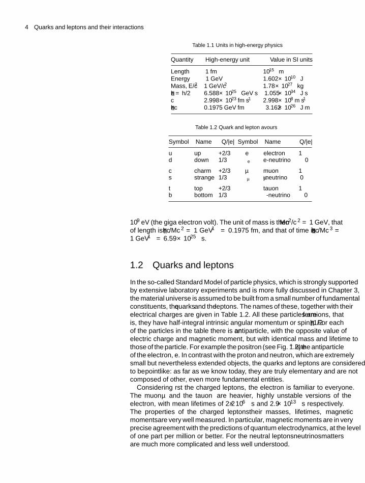
First we should note the units employed in the study of the fundamentalquark and lepton constituents of matter. The unit of length is the femtometer(1 fm = 10−15 m), an appropriate unit because, for example, the charge radiusof a composite particle such as a proton is 0.8 fm. The typical energy scale is thegiga electron volt (1 GeV = 109 eV); for example, the mass energy equivalentof a proton is Mpc2 = 0.938 GeV. Table 1.1 lists the units employed in high-energy physics, together with their equivalents in SI units. A list of appropriatephysical constants is given in Appendix A.
In the description of particle interactions at the quantum level, the quantitiesh = h/2π and c frequently occur, and it is convenient to employ so-callednatural units, which set h = c = 1. Having chosen these two units, we arefree to specify just one more unit, which is taken as that of energy, the GeV =
4 Quarks and leptons and their interactions
Table 1.1 Units in high-energy physics
Quantity High-energy unit Value in SI units
Length 1 fm 10−15 mEnergy 1 GeV 1.602 × 10⁻¹⁰ JMass, E/c2 1 GeV/c2 1.78 × 10⁻²⁷ kgh = h/2π 6.588 × 10⁻²⁵ GeV s 1.055 × 10⁻³⁴ J sc 2.998 × 10²³ fm s−1 2.998 × 10⁸ m s−1
hc 0.1975 GeV fm 3.162 × 10⁻²⁶ J m
Table 1.2 Quark and lepton flavours
Symbol Name Q/|e| Symbol Name Q/|e|u up +2/3 e electron −1d down −1/3 νe e-neutrino 0
c charm +2/3 μ muon −1s strange −1/3 νμ μ-neutrino 0
t top +2/3 τ tauon −1b bottom −1/3 ντ τ-neutrino 0
109 eV (the giga electron volt). The unit of mass is then Mc2/c2 = 1 GeV, thatof length is hc/Mc2 = 1 GeV−1 = 0.1975 fm, and that of time is hc/Mc3 =1 GeV−1 = 6.59 × 10⁻²⁵ s.
1.2 Quarks and leptons
In the so-called Standard Model of particle physics, which is strongly supportedby extensive laboratory experiments and is more fully discussed in Chapter 3,the material universe is assumed to be built from a small number of fundamentalconstituents, the quarks and the leptons. The names of these, together with theirelectrical charges are given in Table 1.2. All these particles are fermions, thatis, they have half-integral intrinsic angular momentum or spin, 1/2h. For eachof the particles in the table there is an antiparticle, with the opposite value ofelectric charge and magnetic moment, but with identical mass and lifetime tothose of the particle. For example the positron (see Fig. 1.2) e+ is the antiparticleof the electron, e−. In contrast with the proton and neutron, which are extremelysmall but nevertheless extended objects, the quarks and leptons are consideredto be pointlike: as far as we know today, they are truly elementary and are notcomposed of other, even more fundamental entities.
Considering first the charged leptons, the electron is familiar to everyone.The muon μ and the tauon τ are heavier, highly unstable versions of theelectron, with mean lifetimes of 2.2 × 10⁻⁶ s and 2.9 × 10⁻¹³ s respectively.The properties of the charged leptons—their masses, lifetimes, magneticmoments—are very well measured. In particular, magnetic moments are in veryprecise agreement with the predictions of quantum electrodynamics, at the levelof one part per million or better. For the neutral leptons—neutrinos—mattersare much more complicated and less well understood.
1.2 Quarks and leptons 5
n beam
n beam
(a)
(b)
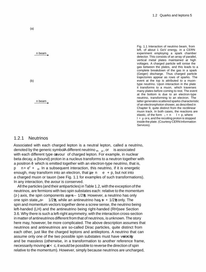
Fig. 1.1 Interaction of neutrino beam, fromleft, of about 1 GeV energy, in a CERNexperiment employing a spark chamberdetector. This consists of an array of parallel,vertical metal plates maintained at highvoltages. A charged particle will ionise thegas between the plates, and this leads to acomplete breakdown of the gas in a spark(Geiger) discharge. Thus charged particletrajectories appear as rows of sparks. Theevent at the top is attributed to a muon-type neutrino. Upon interaction in the plateit transforms to a muon, which traversesmany plates before coming to rest. The eventat the bottom is due to an electron-typeneutrino, transforming to an electron. Thelatter generates scattered sparks characteristicof an electron–photon shower, as described inChapter 9, quite distinct from the rectilinearmuon track. In both cases, the reactions are‘elastic’, of the form νl + n → l + p, wherel = μ or e, and the recoiling proton is stoppedinside the plate. (Courtesy CERN InformationServices).
1.2.1 Neutrinos
Associated with each charged lepton is a neutral lepton, called a neutrino,denoted by the generic symbol ν. A different neutrino νe, νμ, or ντ is associatedwith each different type or flavour of charged lepton. For example, in nuclearbeta decay, a (bound) proton in a nucleus transforms to a neutron together witha positron e+ which is emitted together with an electron-type neutrino, that is,p → n + e+ + νe. In a subsequent interaction, this neutrino, if it is energeticenough, may transform into an electron, that is, νe + n → e− + p, but not intoa charged muon or tauon (see Fig. 1.1 for examples of such transformations).In any interaction, the flavour is conserved.
All the particles (and their antiparticles) in Table 1.2, with the exception of theneutrinos, are fermions with two spin substates each: relative to the momentum(z-) axis, the spin components are sz = ±1/2h. However, a neutrino has onlyone spin state, sz = −1/2h, while an antineutrino has sz = +1/2h only. Thespin and momentum vectors together define a ‘screw sense’, the neutrino beingleft-handed (LH) and the antineutrino being right-handed (RH)—see Section3.6. Why there is such a left-right asymmetry, with the interaction cross-sectionin matter of antineutrinos different from that of neutrinos, is unknown. The storyhere may, however, be more complicated. The above description assumes thatneutrinos and antineutrinos are so-called Dirac particles, quite distinct fromeach other, just like the charged leptons and antileptons. A neutrino that canassume only one of the two possible spin substates must have velocity v = cand be massless (otherwise, in a transformation to another reference frame,necessarily moving at v < c, it would be possible to reverse the direction of spinrelative to the momentum). However, simply because neutrinos are uncharged,
6 Quarks and leptons and their interactions
the other possibility is that neutrinos are their own antiparticles. These so-called ‘Majorana’ neutrinos occur in spin-up and spin-down substates, labelled‘neutrino’ and ‘antineutrino’ in the Dirac picture. Unfortunately, experimentsat the present time are unable to differentiate between these two prescriptions.In Chapters 4 and 6 we describe how massive Majorana neutrinos have beeninvoked in a mechanism to account for the baryon–antibaryon asymmetry inthe universe, which is one of the big puzzles in cosmology. However, becauseof common usage, and except when we specifically discuss Majorana particles,we will speak of neutrinos and antineutrinos as particle and antiparticle.
To further complicate matters, it turns out that, while the charged leptons aredescribed by wavefunctions which are unique mass eigenstates, the neutrinosare not, but superpositions of mass eigenstates, with slightly different massvalues and, for a given momentum therefore, slightly different velocities. Asa consequence, in travelling through empty space, phase differences developas the different mass eigenstates get ‘out of step’, appearing as oscillationsin the neutrino flavour between νe, νμ, and ντ . Neutrino oscillations arediscussed fully in Chapters 4 and 9; they measure the mass differences betweenthe eigenstates, and these are tiny, of order 0.1 eV/c2. The correspondingwavelengths of the flavour oscillations are extremely long—100’s or 1000’sof kilometres for neutrino energies of order 1 GeV. Neutrino oscillations hadactually been proposed in 1964, but because of these tiny mass differences, itwas to take some 30 years of research—and 60 years after Pauli first postulatedthe neutrino – to discover them. Direct measurements of neutrino mass (ratherthan mass differences) shown in Table 1.3, obtained, for example, in the caseof νe from the shape of the end-point in tritium beta decay, give upper limitswhich at present are much larger.
The neutrinos turn out to be of great importance in the cosmology of the earlyuniverse, as discussed later. Next to the microwave photons constituting the relicelectromagnetic radiation from the Big Bang (411 per cm3 throughout space),relic neutrinos are by far the most abundant particles in the universe. Theirnumber density of 340 per cm3 is to be compared with only about 1.25 × 10⁻⁷
protons, neutrons, or electrons per cm3. As discussed in detail in Chapter 8,it seems that in the primordial universe during its first 400,000 years, beforeradiation decoupled from matter, neutrinos played an important and indeedcrucial role in the development of cosmic structures on the large scales ofgalaxy clusters and superclusters.
1.2.2 Quark flavours
The quarks in Table 1.2 have fractional electric charges, of +2|e|/3 and −|e|/3where |e| is the numerical value of the electron charge. As for the chargedleptons, the masses increase as we go down the table (see also Tables 1.3and 1.4). Apart from charge and spin, the quarks, like the leptons, have an extrainternal degree of freedom, again called the flavour. The odd names for thevarious quark flavours—‘up’, ‘down’, ‘charm’, etc.—have arisen historically.Just as for the leptons, the six flavours of quark are arranged in three doublets,the components of which differ by one unit of electric charge.
While the leptons exist as free particles, the quarks do not (but see theremarks later on the quark–gluon plasma). It is a peculiarity of the strong forcebetween the quarks that, at normal energies, they are always found associated
1.2 Quarks and leptons 7
in quark composites called hadrons. These are of two types: baryons consist ofthree quarks, QQQ, while mesons consist of a quark–antiquark pair, QQ. Forexample,
Proton = u u d Neutron = d d u
Pion π+ = u d π− = u d
The common material of the world today is built from u and d quarks, formingthe protons and neutrons of atomic nuclei, which together with the electrons e−form atoms and molecules. The heavier quarks c, s, t, and b are also observed toform baryon composites such as sud, sdc, … and mesons such as bb, cc, cb, . . . ,but these heavy hadrons are all highly unstable and decay rapidly to statescontaining u and d quarks only. Likewise the heavier charged leptons μ andτ decay to electrons and neutrinos. These heavy quarks and leptons can beproduced in collisions at laboratory accelerators, or naturally in the atmosphereas a result of collisions of high-energy cosmic rays. However, they appearto play only a minor role in today’s relatively cold universe. For example,while several hundred high-energy muons (coming down to earth as secondarycomponents of the cosmic rays) pass through everyone each minute, this is atrivially small number compared with the human tally of electrons, of order1028. The cosmic ray muons add to the natural levels of radiation, comingfrom radioactive elements in the ground and the atmosphere, and presumablytherefore they make a contribution to the natural gene mutation rate from theeffects of radiation.
Of course we believe that these heavier flavours of quark and lepton wouldhave been as prolific as the light ones at a very early, intensely hot stage ofthe Big Bang, when the temperature was such that the mean thermal energykT far exceeded the mass energy of these particles. Indeed, it is clear that thetype of universe we inhabit today must have depended very much, in its initialevolution, on these heavier fundamental particles—as well as on new forms ofmatter and energy, which (so far) cannot be produced at accelerators and theexistence of which we deduce from astronomical observations.
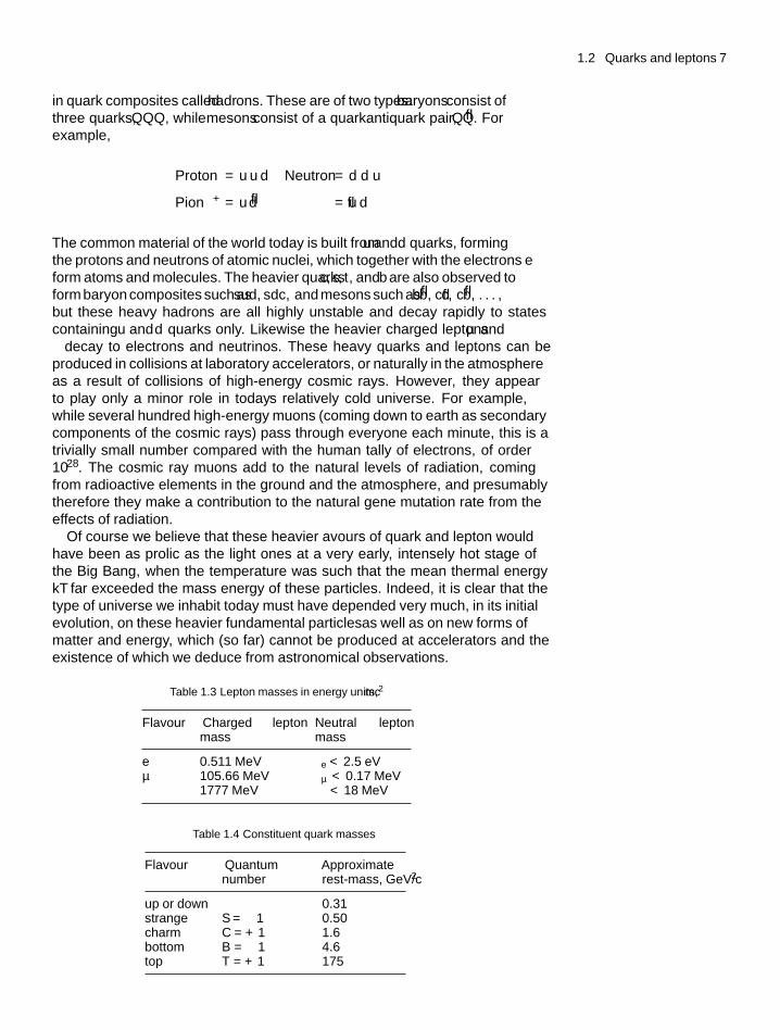
Table 1.3 Lepton masses in energy units, mc2
Flavour Charged leptonmass
Neutral leptonmass
eμτ
0.511 MeV105.66 MeV1777 MeV
νe < 2.5 eVνμ < 0.17 MeVντ < 18 MeV
Table 1.4 Constituent quark masses
Flavour Quantumnumber
Approximaterest-mass, GeV/c2
up or downstrangecharmbottomtop
—S = −1C = +1B = −1T = +1
0.310.501.64.6175
8 Quarks and leptons and their interactions
The masses of the quarks and leptons are given in Tables 1.3 and 1.4. Themasses shown for neutrinos in Table 1.3 are upper limits deduced from energyand momentum conservation in decays involving neutrinos (e.g., from thekinematics of pion decay π → μ + νμ, or from tritium beta decay 3H →3He + e− + ve). As already noted above, evidence from neutrino flavouroscillations indicates neutrino mass differences, and by inference the massesthemselves, which are much less than these limits, and in the region of 0.1 eV/c2.Upper limits of ∼0.5 eV/c2 for the neutrino masses, summed over all flavours,are also obtained from analyses of the spectrum of density fluctuations ofmicrowave radiation in the early universe, and from galaxy surveys, describedin Chapter 8.
As discussed below, the quarks are held together in hadrons by the gluoncarriers of the strong force, and the ‘constituent’ quark masses in Table 1.4include such quark binding effects. The u and d quarks have nearly equal masses(each of about one third that of the nucleon) as indicated by the smallness of theneutron–proton mass difference of 1.3 MeV/c2. Isospin symmetry in nuclearphysics results from this near coincidence in the light quark masses.
High-energy scattering experiments often involve ‘close’ collisions betweenthe quarks. In this case, the quarks can be temporarily separated from theirretinue of gluons, and the so-called current quark masses which then apply aresmaller than the constituent masses by about 0.30 GeV/c2. So the current u andd quark masses are a few MeV/c2 only. In this regard, the smallness of theneutron–proton mass difference is not such a coincidence.
In the strong interactions between the quarks, the flavour quantum numberis conserved, and is denoted by the quark symbol in capitals. For example, astrange s quark has a strangeness quantum number S = −1, while a strangeantiquark s has S = +1. Thus, in a collision between hadrons containing u andd quarks only, heavier quarks can be produced, but only as quark–antiquarkpairs, so that the net flavour is conserved. In weak interactions, on the contrary,the quark flavour may change, for example, one can have transitions of the form�S = ±1, �C = ±1, etc. As an example, a baryon called the lambda hyperonof S = −1 decays to a proton and a pion, � → p + π−, with a mean lifetimeof 2.6 × 10⁻¹⁰ s, typical of a weak interaction of �S = +1. This decay wouldbe expressed as sud → uud + du in quark nomenclature.
A few words are appropriate here about the practical attainment in thelaboratory of high mass scales in high-energy particle physics. The completionof Table 1.2 of fermions and Table 1.5 of bosons took over 40 years of thetwentieth century, as bigger and more energetic particle accelerators were
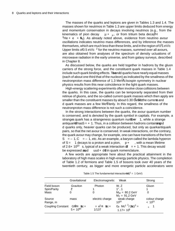
Table 1.5 The fundamental interactions (Mc2 = 1 GeV)
Gravitational Electromagnetic Weak Strong
Field boson Graviton Photon W , Z GluonSpin/Parity 2+ 1− 1+, 1− 1−Mass 0 0 MW = 80.2 GeV 0
MZ = 91.2 GeVSource mass electric charge weak charge colour chargeRange, m ∞ ∞ 10−18 < 10−15
Coupling Constant GM 2/4πhc =5 × 10−40
α = e2/4πhc =1/137
GF(Mc2)2
/(hc)3 =1.17 × 10⁻⁵
αs ≤ 1
1.4 Antiparticles 9
able to excite production of more and more massive fundamental states. Thefirst evidence for the existence of the lighter quarks u, d , s appeared in the1960s, from experiments at the CERN PS (Geneva) and Brookhaven AGS(Long Island) proton synchrotrons, with beam energies of 25–30 GeV, aswell as the 25 GeV electron linear accelerator at SLAC, Stanford. The weakbosons W and Z , with masses of 80 and 90 GeV/c2 were first observedin 1983 at the CERN proton–antiproton collider with oppositely circulatingbeams of energy 270 GeV (see Fig. 1.6). The most massive particle so farproduced, the top quark of mass 175 GeV/c2, was first observed in 1995 atthe Fermilab proton–antiproton collider (Chicago), with 900 GeV energy ineach beam.
1.3 Fermions and bosons: the spin-statisticstheorem; supersymmetry
As stated above, the fundamental particles consist of half-integer spin fermions,the quarks and leptons, the interactions of which are mediated, as describedbelow, by integer spin bosons. The distinction between the two types isunderlined by the spin-statistics theorem. This specifies the behaviour of anensemble of identical particles, described by some wave function ψ, when anytwo particles, say 1 and 2, are interchanged. The probability |ψ|2 cannot bealtered by the interchange, since the particles are indistinguishable, so underthe operation, ψ → ±ψ. The rule is as follows:
Identical bosons: under interchange ψ → +ψ SymmetricIdentical fermions: under interchange ψ → −ψ Antisymmetric
Suppose, for example, that it were possible to put two identical fermions inthe same quantum state. Then under interchange, ψ would not change sign,since the particles are indistinguishable. However, according to the above ruleψ must change sign. Hence two identical fermions cannot exist in the samequantum state—the famous Pauli Principle. On the other hand, there are norestrictions on the number of identical bosons in the same quantum state, anexample of this being the laser.
One important development in connection with theories unifying thefundamental interactions at very high mass scales, has been the postulate ofa fermion–boson symmetry called supersymmetry. For every known fermionstate there is assigned a boson partner, and for every boson a fermion partner.The reasons for this postulate are discussed in Chapter 3, and a list of proposedsupersymmetric particles given in Table 3.2. At this point we content ourselveswith the remark that if they exist, supersymmetric particles created in the earlyuniverse could be prime candidates for the mysterious dark matter which, as weshall see in Chapter 7, constitutes the bulk of the material universe. However,at the present time there is no direct experimental evidence for the existence ofsupersymmetric particles.
1.4 Antiparticles
In 1931, Dirac wrote down a wave equation describing an electron, which wasfirst order in both space and time coordinates, and had four solutions. Two of
10 Quarks and leptons and their interactions
these were for the electron, and corresponded to the two possible spin substateswith projections sz = +(1/2)h and −(1/2)h along the quantization axis. Theother two solutions were attributed to the antiparticle, with similar propertiesto the electron except for the opposite value of the electric charge. Thesepredictions followed from the two great conceptual advances in twentieth-century physics, namely the classical theory of relativity and the quantummechanical description of atomic and subatomic phenomena.
The relativistic relation connecting energy E, momentum p, and rest-mass mis (see the section on relativistic kinematics in Chapter 2)
E2 = p2c2 + m2c4 (1.1)
From this equation we see that the total energy can in principle assume bothnegative and positive values
E = ±√
p2c2 + m2c4 (1.2)
While in classical mechanics negative energies appear to be meaningless, inquantum mechanics we represent a stream of electrons travelling along thepositive x-axis by the plane wavefunction
ψ = A exp [−i(Et − px)/h] (1.3)
where the angular frequency is ω = E/h, the wavenumber is k = p/h, andA is a normalization constant. As t increases, the phase (Et – px) advances inthe direction of positive x. However, (1.3) can equally well represent a particleof energy −E and momentum −p travelling in the negative x-direction andbackwards in time, that is, replacing Et by (−E)(−t) and px by (−p)(−x):
E > 0 E < 0
t1 → t2 t1 ← t2 (t2 > t1)
A stream of negatively charged electrons flowing backwards in time isequivalent to a positive charge flowing forwards, thus with E > 0. Hence thenegative energies are formally connected with the existence of a positive energyantiparticle e+, the positron. This particle was first observed by Anderson in1932, quite independently of Dirac’s prediction (see Fig. 1.2). The existence ofantiparticles is a general property of both fermions and bosons, but for fermionsonly there is a conservation rule. One can define a fermion number, +1 for afermion and −1 for an antifermion and postulate that the total fermion numberis conserved. Thus fermions can only be created or destroyed in particle–antiparticle pairs, such as e+e− or QQ. For example, a γ-ray, if it has energyE > 2mc2 where m is the electron mass, can create a pair (in the presence ofan atom to conserve momentum), and an e+e− pair can annihilate to γ-rays.As another example, in massive stars reaching the supernova phase, fermionnumber conserving reactions such as e+ + e− → v + v are expected to becommonplace.
At the energies available in the laboratory, and certainly today in our relativelycold universe, leptons and baryons are strictly conserved. Thus a charged lepton(e−, μ−, or τ−) is given a lepton number L = +1, while their antiparticles are
1.5 The fundamental interactions: boson exchange 11
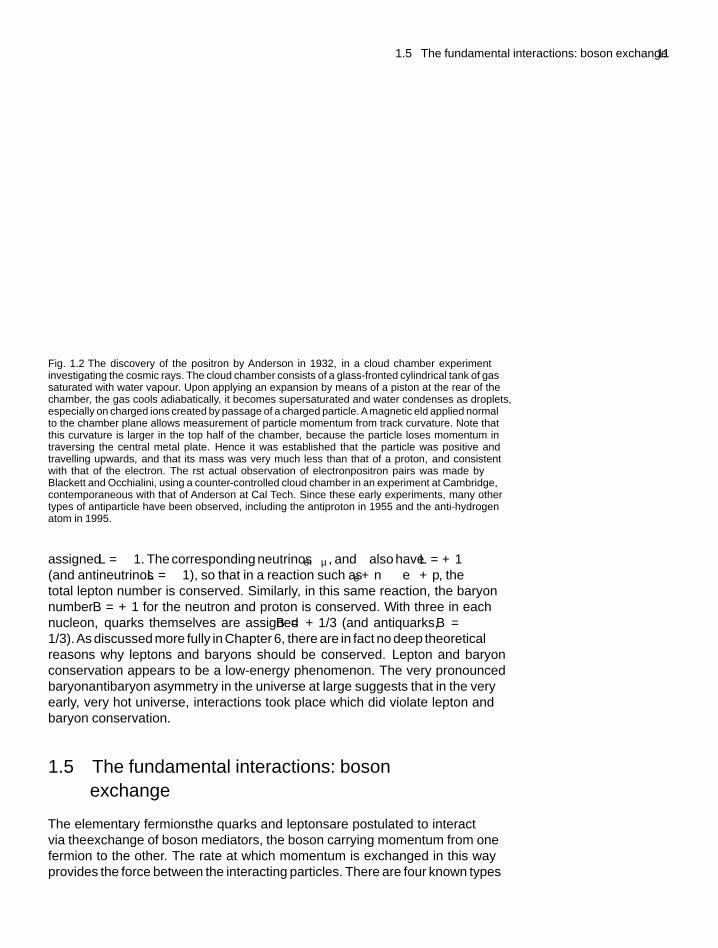
Fig. 1.2 The discovery of the positron by Anderson in 1932, in a cloud chamber experimentinvestigating the cosmic rays. The cloud chamber consists of a glass-fronted cylindrical tank of gassaturated with water vapour. Upon applying an expansion by means of a piston at the rear of thechamber, the gas cools adiabatically, it becomes supersaturated and water condenses as droplets,especially on charged ions created by passage of a charged particle. Amagnetic field applied normalto the chamber plane allows measurement of particle momentum from track curvature. Note thatthis curvature is larger in the top half of the chamber, because the particle loses momentum intraversing the central metal plate. Hence it was established that the particle was positive andtravelling upwards, and that its mass was very much less than that of a proton, and consistentwith that of the electron. The first actual observation of electron–positron pairs was made byBlackett and Occhialini, using a counter-controlled cloud chamber in an experiment at Cambridge,contemporaneous with that of Anderson at Cal Tech. Since these early experiments, many othertypes of antiparticle have been observed, including the antiproton in 1955 and the anti-hydrogenatom in 1995.
assigned L = −1. The corresponding neutrinos νe, νμ, and ντ also have L = +1(and antineutrinos L = −1), so that in a reaction such as νe + n → e− + p, thetotal lepton number is conserved. Similarly, in this same reaction, the baryonnumber B = +1 for the neutron and proton is conserved. With three in eachnucleon, quarks themselves are assigned B = +1/3 (and antiquarks, B =−1/3). As discussed more fully in Chapter 6, there are in fact no deep theoreticalreasons why leptons and baryons should be conserved. Lepton and baryonconservation appears to be a low-energy phenomenon. The very pronouncedbaryon–antibaryon asymmetry in the universe at large suggests that in the veryearly, very hot universe, interactions took place which did violate lepton andbaryon conservation.
1.5 The fundamental interactions: bosonexchange
The elementary fermions—the quarks and leptons—are postulated to interactvia the exchange of boson mediators, the boson carrying momentum from onefermion to the other. The rate at which momentum is exchanged in this wayprovides the force between the interacting particles. There are four known types
12 Quarks and leptons and their interactions
of interaction, each with its characteristic boson exchange particle. They are asfollows:
• The electromagnetic interaction occurs between all types of chargedparticle, and is brought about by exchange of a photon, with spin 1and zero mass.
• The strong interactions occur between the quarks, via exchange of thegluon, a particle again with spin 1 and zero mass. Such interactionsare responsible not only for the binding of quarks in hadrons butalso for the force holding neutrons and protons together in atomicnuclei.
• The weak interactions take place between all types of quark and lepton.They are mediated by the exchange of weak bosons,W ± and Z0. Theseparticles are also of spin 1 but have masses of 80 and 91 GeV respectively.Weak interactions are responsible for radioactive beta decay ofnuclei.
• The gravitational interactions take place between all forms of matter orradiation. They are mediated by the exchange of gravitons, of zero massbut spin 2.
For orientation on the magnitudes involved, the relative strengths of thedifferent forces between two protons when just in contact are approximately
Strong Electromagnetic Weak Gravitational1 10−2 10−7 10−39 (1.4)
The weakness of gravity, compared with electromagnetism, is of courseknown to everyone from earliest childhood. As you fall down, you accelerateunder the gentle force of gravity, but only on hitting the ground do you realisethe enormously larger electromagnetic forces between molecules. Despite suchdifferences, numerous attempts have been made over the years to find a unifiedtheory, a so-called theory of everything. It turns out that the electromagneticand weak interactions are in fact different aspects of a single electroweakinteraction, as described below. The possibility of grander unification schemesand the reasons for them are discussed in Chapter 4.
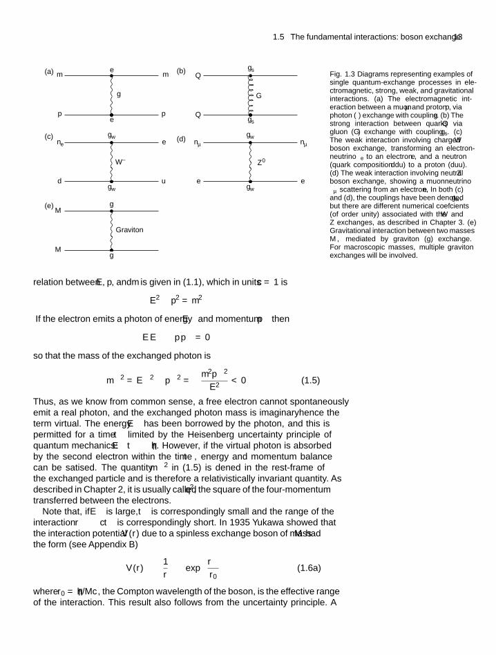
Figure 1.3 shows diagrams depicting the above exchange processes, andTable 1.5 lists some of the properties of the interactions. In these diagrams(called in a more sophisticated form, Feynman diagrams after their inventor)solid lines entering or leaving the boundaries represent real particles—usually,quarks or leptons—with time flowing from left to right. The arrows along theselines indicate the direction of fermion number flow (see Fig. 1.9). An arrowindicating an electron flowing backwards in time is equivalent to a positron(i.e. antifermion) moving forwards: the convention is to use such time-reversedarrows for antiparticles.
Wavy, curly, or broken lines run between the vertices where the exchangeinteractions take place, and they represent the mediating bosons, which arevirtual particles, that is, they carry energy and momentum such that the massdoes not correspond to that of the free particle. To understand this, consider,for example, an electron of total energy E, momentum p, and mass m beingscattered as another electron absorbs the exchanged photon. The relativistic
1.5 The fundamental interactions: boson exchange 13
(b)(a)
(c)
(e)
(d)
g G
m m
ne nμ nμ
e
ep p
Q
Q
gs
gs
d
e
u
W ±
e e
gwgw
gwgw
Z0
M
M
g
g
Graviton
Fig. 1.3 Diagrams representing examples ofsingle quantum-exchange processes in ele-ctromagnetic, strong, weak, and gravitationalinteractions. (a) The electromagnetic int-eraction between a muon μ and proton p, viaphoton (γ) exchange with coupling e. (b) Thestrong interaction between quarks Q viagluon (G) exchange with coupling gs. (c)The weak interaction involving charged Wboson exchange, transforming an electron-neutrino νe to an electron e, and a neutron(quark composition ddu) to a proton (duu).(d) The weak interaction involving neutral Zboson exchange, showing a muon–neutrinoνμ scattering from an electron, e. In both (c)and (d), the couplings have been denoted gw,but there are different numerical coefficients(of order unity) associated with the W andZ exchanges, as described in Chapter 3. (e)Gravitational interaction between two massesM , mediated by graviton (g) exchange.For macroscopic masses, multiple gravitonexchanges will be involved.
relation between E, p, and m is given in (1.1), which in units c = 1 is
E2 − p2 = m2
If the electron emits a photon of energy �E and momentum �p then
E �E − p �p = 0
so that the mass of the exchanged photon is
�m2 = �E2 − �p2 = −m2�p2
E2< 0 (1.5)
Thus, as we know from common sense, a free electron cannot spontaneouslyemit a real photon, and the exchanged photon mass is imaginary—hence theterm virtual. The energy �E has been ‘borrowed’ by the photon, and this ispermitted for a time �t limited by the Heisenberg uncertainty principle ofquantum mechanics: �E �t ∼ h. However, if the virtual photon is absorbedby the second electron within the time �t, energy and momentum balancecan be satisfied. The quantity �m2 in (1.5) is defined in the rest-frame ofthe exchanged particle and is therefore a relativistically invariant quantity. Asdescribed in Chapter 2, it is usually called q2, the square of the four-momentumtransferred between the electrons.
Note that, if �E is large, �t is correspondingly small and the range of theinteraction �r ≈ c�t is correspondingly short. In 1935 Yukawa showed thatthe interaction potential V (r) due to a spinless exchange boson of mass M hadthe form (see Appendix B)
V (r) ∝(
1
r
)exp
(−r
r0
)(1.6a)
where r0 = h/Mc, the Compton wavelength of the boson, is the effective rangeof the interaction. This result also follows from the uncertainty principle. A
14 Quarks and leptons and their interactions
boson of mass M can exist as a virtual particle for a time �t ∼ h/Mc2, duringwhich it can travel at most a distance c �t ∼ h/Mc. The W and Z bosonshave large masses and so the range r0 is very short (of order 0.0025 fm). Thisis the reason that weak interactions are so much feebler than electromagnetic.The free photon associated with electromagnetism has rest-mass M = 0 andr0 = ∞ so that the value of �E of the virtual photon can be arbitrarily smalland the range of the interaction can therefore be arbitrarily large.
Instead of discussing the range of a static interaction, these features can betaken into account in a scattering process by defining a so-called propagator,measuring the amplitude for scattering with a momentum transfer q. Neglectingspin, this has the general form, following from the Yukawa potential (seeAppendix B)
F(q2) = 1(−q2 + M 2) (1.6b)
where q2 = �E2 − �p2 is the (negative) four-momentum transfer squaredin (1.5) and M is the (free particle) rest-mass of the exchanged boson. Sofor photons M = 0, for a weak boson M = MW , and so on. The square ofF(q2) enters into the cross-section describing the probability of the interaction,as discussed below. As an example, for Coulomb scattering M = 0 andthe differential cross-section dσ/dq2 varies as 1/q4, as given by the famousRutherford scattering formula.
1.6 The boson couplings to fermions
1.6.1 Electromagnetic interactions
Apart from the effect of the boson propagator term, the strength of a particularinteraction is determined by the coupling strength of the fermion (quark orlepton) to the mediating boson. For electromagnetic interactions, shown inFig. 1.3(a), the coupling of the photon to the fermion is denoted by the electriccharge |e| (or fraction of it, in the case of a quark), and the product of thecouplings of two fermions, each of charge |e|, to each other is
e2 = 4παhc,
more usually written as 4πα in natural units with h = c = 1. Hereα ≈ 1/137 is the dimensionless fine structure constant. The cross-section orrate of a particular interaction is proportional to the square of the transitionamplitude. This amplitude is proportional to the product of the vertex factorsand the propagator term, that is, α/|q2| for the electromagnetic interaction,corresponding to a factor α2/|q4| for the rate.
1.6.2 Strong colour interactions
For strong interactions, as in Fig. 1.3(b), the coupling of the quark to the gluonis denoted gs with g2
s = 4παs. Typically, αs is a number of order unity. Whilein the electromagnetic interactions there are just two types of electric charge,denoted by the symbols + and −, as in Fig. 1.4(a), the interquark interactionsinvolve six types of strong charge. This internal degree of freedom is called
1.6 The boson couplings to fermions 15
Q
Q
Q
(a)
(c)
(b)
– –
+ +
g
r b
b r
G rb
QQQ Q Q
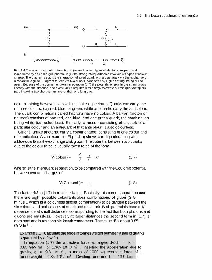
Fig. 1.4 The electromagnetic interaction in (a) involves two types of electric charge, + and − andis mediated by an uncharged photon. In (b) the strong interquark force involves six types of colourcharge. The diagram depicts the interaction of a red quark with a blue quark via the exchange ofa red–antiblue gluon. Diagram (c) depicts two quarks, connected by a gluon ‘string’, being pulledapart. Because of the confinement term in equation (1.7) the potential energy in the string growslinearly with the distance, and eventually it requires less energy to create a fresh quark–antiquarkpair, involving two short strings, rather than one long one.
colour (nothing however to do with the optical spectrum). Quarks can carry oneof three colours, say red, blue, or green, while antiquarks carry the anticolour.The quark combinations called hadrons have no colour. A baryon (proton orneutron) consists of one red, one blue, and one green quark, the combinationbeing white (i.e. colourless). Similarly, a meson consisting of a quark of aparticular colour and an antiquark of that anticolour, is also colourless.
Gluons, unlike photons, carry a colour charge, consisting of one colour andone anticolour. As an example, Fig. 1.4(b) shows a red quark r interacting witha blue quark b via the exchange of a rb gluon. The potential between two quarksdue to the colour force is usually taken to be of the form
V (colour) = −(
4
3
)αs
r+ kr (1.7)
where r is the interquark separation, to be compared with the Coulomb potentialbetween two unit charges of
V (Coloumb) = −α
r(1.8)
The factor 4/3 in (1.7) is a colour factor. Basically this comes about becausethere are eight possible colour–anticolour combinations of gluon (32 = 9,minus 1 which is a colourless singlet combination) to be divided between thesix colours and anti-colours of quark and antiquark. Both potentials have a 1/rdependence at small distances, corresponding to the fact that both photons andgluons are massless. However, at larger distances the second term in (1.7) isdominant and is responsible for quark confinement. The value of k is about 0.85GeV fm−1.
Example 1.1 Calculate the force in tonnes weight between a pair of quarksseparated by a few fm.
In equation (1.7) the attractive force at large r is dV /dr = k =0.85 GeV fm−1 or 1.36 × 10⁵ J m−1. Inserting the acceleration due togravity, g = 9.81 m s−2, a mass of 1000 kg exerts a force of 1tonne-weight = 9.8 × 10³ J m−1. Dividing, one finds k = 13.9 tonnes
16 Quarks and leptons and their interactions
weight—a great deal for those tiny quarks, each weighing less than10−24 gm.
Because gluons carry a colour charge (unlike photons which are uncharged)there is a strong gluon–gluon interaction. Thus the ‘lines of colour force’between a pair of quarks, analogous to the lines of electric field between apair of charges, are pulled out into a tube or string. In Fig. 1.4(c) such a gluon‘string’ is depicted connecting a quark–antiquark pair. If one tries to pull apartthe two quarks, the energy required to do so grows linearly with the stringlength as in (1.7), and eventually it requires less energy to produce anotherquark–antiquark pair, thus involving two short strings instead of one long one.Thus even the most violent efforts to separate quarks just result in productionof lots of quark–antiquark pairs (mesons).
We may note at this point a peculiar property of the quark and lepton quantumnumbers. Each of the three ‘families’ consists of a doublet of quarks of charge+2/3|e| and −1/3|e| respectively, and a pair of leptons with charges –1|e| and0. If allowance is made for the colour degree of freedom, the total charge ofthe quarks is 3 × (2/3 − 1/3) |e| = +1|e| per family, while for the leptonsit is (−1 + 0)|e| = −1|e|. This is true for each family, so the total electriccharge of the fermions is zero. In fact it turns out that an important quantityis the square of the electric charge multiplied by a quantity called the axial–vector coupling, which comes in with the same value but opposite signs forthe charged and neutral leptons, and for the charge +2/3 and charge −1/3quarks. Then in units of |e|2 the total amounts to [(0)2 − (−1)2] = −1 forthe leptons, and 3 × [(+2/3)2 − (−1/3)2] = +1 for the quarks, which againadds to zero. This turns out to be a crucial property, in making the theory freeof so-called ‘triangle anomalies’ which, if they were not cancelled out, wouldspoil the renormalizability of the theory, discussed in Chapter 3. In fact, thefundamental reason for the existence of three families which are, so to speak,‘carbon copies’ of one another, is at present unknown.
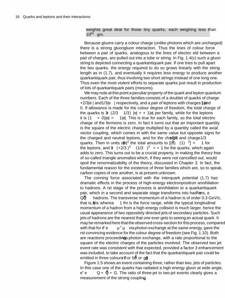
The confining force associated with the interquark potential (1.7) hasdramatic effects in the process of high-energy electron–positron annihilationto hadrons. A first stage of the process is annihilation to a quark–antiquarkpair, which in a second and separate stage transforms into hadrons, e+e− →QQ → hadrons. The transverse momentum of a hadron is of order 0.3 GeV/c,that is, h/a where a ∼ 1 fm is the force range, while the typical longitudinalmomentum of a hadron from a high-energy collision is much larger, hence theusual appearance of two oppositely directed ‘jets’ of secondary particles. Such‘jets’ of hadrons are the nearest that one ever gets to ‘seeing’ an actual quark. Itmay be remarked here that the observed cross-section for this process, comparedwith that for e+e− → μ+μ− via photon exchange at the same energy, gave thefirst convincing evidence for the colour degree of freedom (see Fig. 1.10). Bothare reactions proceeding via photon exchange, with a rate proportional to thesquare of the electric charges of the particles involved. The observed two jetevent rate was consistent with that expected, provided a factor 3 enhancementwas included, to take account of the fact that the quark–antiquark pair could beemitted in three colours
(rr or bb or gg
).
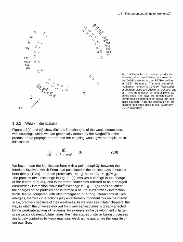
Figure 1.5 shows an event containing three, rather than two, jets of particles.In this case one of the quarks has radiated a high-energy gluon at wide angle,e+e− → Q + Q + G. The ratio of three-jet to two-jet events clearly gives ameasurement of the strong coupling αs.
1.6 The boson couplings to fermions 17
2202481063
36837
25
41
259304
18211110030
9
31
79
24
368
821
1052618880
123
275
344
3665
79
99271
2.23.915
16
3.01819
1.520
4.221
2.422
4.5
276.4
7.3
6
3.7
4
2.8
3
2.2 1
3.3
426.2
40
4.8
37
3.9
36
2.5
35
3.3
34
2.8
33
–0.7
2
4.217
x
y
z
Fig. 1.5 Example of hadron productionfollowing e+e− annihilation observed inthe JADE detector at the PETRA colliderat DESY, Hamburg. The total centre-of-momentum energy is 30 GeV. Trajectoriesof charged pions are shown as crosses, andof γ-rays from decay of neutral pions asdotted lines. The γ-rays are detected whenthey produce electron–photon showers in leadglass counters. Note the collimation of thehadrons into three distinct ‘jets’. (CourtesyDESY laboratory).
1.6.3 Weak Interactions
Figure 1.3(c) and (d) show the W and Z exchanges of the weak interactions,with couplings which we can generically denote by the symbol gw. Thus theproduct of the propagator term and the coupling would give an amplitude inthis case of
Ltq2→0
g2w(−q2 + Mw2
) ≡ GF (1.9)
We have made the identification here with a point coupling GF between thefermions involved, which Fermi had postulated in the earliest days of nuclearbeta decay (1934). In those processes |q2| M 2
W so that GF = g2w/M 2
W .The process of W ± exchange in Fig. 1.3(c) involves a change in the chargeof the lepton or quark, and is therefore sometimes referred to as a ‘chargedcurrent’ weak interaction, while the Z0 exchange in Fig. 1.3(d) does not affectthe charges of the particles and is termed a ‘neutral current’ weak interaction.While feeble compared with electromagnetic or strong interactions at GeVenergies, the weak interactions play an extremely important role on the cosmicscale, precisely because of their weakness. As we shall see in later chapters, theway in which the universe evolved from very earliest times is greatly affectedby the weak interactions of neutrinos, for example, in the development of large-scale galaxy clusters. At later times, the initial stages of stellar fusion processesare largely controlled by weak reactions which alone guarantee the long life ofour own Sun.
18 Quarks and leptons and their interactions
1.6.4 Electroweak interactions
As stated above, the electromagnetic and weak interactions are unified. Theelectroweak model was developed in the 1960s, particularly by Glashow (1961),Salam (1967) and Weinberg (1967). Basically what this means is that thecouplings of the W and Z bosons to the fermions are the same as that of thephoton, that is, gw = e. Here for simplicity we have omitted certain numericalfactors of order unity. If one inserts this equality in (1.9) for the limit of low q2,one obtains the expected large masses for the weak bosons:
MW ,Z ∼ e√GF
=√
4πα
GF∼ 100 GeV (1.10)
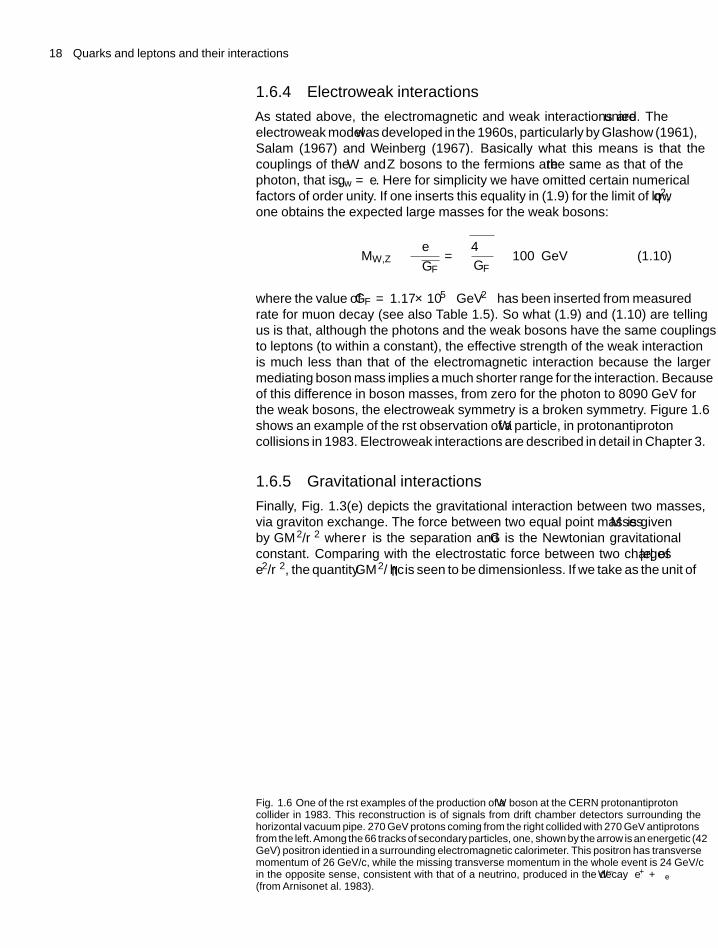
where the value of GF = 1.17×10⁻⁵ GeV−2 has been inserted from measuredrate for muon decay (see also Table 1.5). So what (1.9) and (1.10) are tellingus is that, although the photons and the weak bosons have the same couplingsto leptons (to within a constant), the effective strength of the weak interactionis much less than that of the electromagnetic interaction because the largermediating boson mass implies a much shorter range for the interaction. Becauseof this difference in boson masses, from zero for the photon to 80–90 GeV forthe weak bosons, the electroweak symmetry is a broken symmetry. Figure 1.6shows an example of the first observation of a W particle, in proton–antiprotoncollisions in 1983. Electroweak interactions are described in detail in Chapter 3.
1.6.5 Gravitational interactions
Finally, Fig. 1.3(e) depicts the gravitational interaction between two masses,via graviton exchange. The force between two equal point masses M is givenby GM 2/r2 where r is the separation and G is the Newtonian gravitationalconstant. Comparing with the electrostatic force between two charges |e| ofe2/r2, the quantity GM 2/hc is seen to be dimensionless. If we take as the unit of
Fig. 1.6 One of the first examples of the production of a W boson at the CERN proton–antiprotoncollider in 1983. This reconstruction is of signals from drift chamber detectors surrounding thehorizontal vacuum pipe. 270 GeV protons coming from the right collided with 270 GeV antiprotonsfrom the left.Among the 66 tracks of secondary particles, one, shown by the arrow is an energetic (42GeV) positron identified in a surrounding electromagnetic calorimeter. This positron has transversemomentum of 26 GeV/c, while the missing transverse momentum in the whole event is 24 GeV/cin the opposite sense, consistent with that of a neutrino, produced in the decay W ± → e+ + νe(from Arnison et al. 1983).
1.6 The boson couplings to fermions 19
mass Mc2 = 1 GeV, then
GM 2
4πhc= 5.3 × 10−40 (1.11a)
to be compared with
e2
4πhc= 1
137.036(1.11b)
Thus, for the energy or mass scales of GeV or TeV common in high-energyphysics experiments at accelerators, the gravitational coupling is absolutelynegligible. Of course, on a macroscopic scale, gravity is important andindeed dominant, because it is cumulative, since all particles with energy andmomentum are attracted by their mutual gravitation. Thus the gravitationalforce on a charged particle on the Earth’s surface is the sum of the attractiveeffects of all the matter in the Earth. Since the Earth is electrically neutralhowever, the enormously larger electrical force due to all the protons in theEarth is exactly cancelled by the opposing force due to the electrons.
However, even on sub-atomic scales the gravitational coupling can becomestrong for hypothetical elementary particles of mass equal to the Planck mass,defined as
MPL =(
hc
G
)1/2
= 1.2 × 10¹⁹ GeV
c2(1.12a)
The Planck length is defined as
LPL = h
MPLc= 1.6 × 10⁻³⁵ m (1.12b)
that is, the Compton wavelength of a particle of the Planck mass. Two pointlikeparticles each of the Planck mass and separated by the Planck length wouldtherefore have a gravitational potential energy equal to their rest-masses, soquantum gravitational effects can become important at the Planck scale. Toaccount for the very large value of the Planck mass, or the extreme weakness ofgravity at normal energies, it has been proposed that there are extra dimensionsbeyond the familiar four of space/time, but these are ‘curled up’ to lengths ofthe order of the Planck length, so that they only become effective, and gravitybecomes strong, at Planck energies.
We should emphasize here that, although we can draw a parallel between theinverse square law of force between point charges and point masses, there arequite fundamental differences between the two. First, due to the attractive forcebetween two masses, the latter can acquire momentum and kinetic energy (atthe cost of potential energy), which is equivalent to an increase in the effectivemass through the Einstein relation E = mc2, and thence in the gravitationalforce. For close enough encounters therefore, the force will increase fasterthan 1/r2. Indeed, one gets non-linear effects, which is one of the problemsin formulating a quantum field theory of gravity. The effects of gravitationalfields (including the non-linear behaviour) are enshrined in the Einstein fieldequations of general relativity, which interpret these effects in terms of thecurvature of space caused by the presence of masses.
20 Quarks and leptons and their interactions
Second, it should be noted that in the above we have described gravityon a quantum-exchange basis, just like the other interactions. However, asdiscussed in Chapter 2, gravity is unique in that it cannot be simply treated asanother field operating in normal ‘flat’space. The Equivalence Principle equatesthe gravitational field with an accelerated reference frame, and so in a strongfield, clocks run slow (or timescales are dilated), and lengths are contracted.Time and space, so to speak, get mixed up. Einstein (who of course pre-datedquantum mechanics) treated gravity as a geometrical property of space, andmassive particles then altered the structure of space/time, and attracted oneanother because the space between them was ‘curved’ or ‘warped’. Fine. Buthe then tried for years without success to bring other interactions, for example,electromagnetic interactions, into this picture. Unfortunately, attempts to unifythe different interactions into a ‘theory of everything’, for example in the theorycalled ‘supergravity’, have not got very far.
While for the strong, electromagnetic and weak interactions, there isdirect laboratory evidence for the existence of the mediating bosons—gluons, photons, and weak bosons respectively—so far the direct detection ofgravitational waves (gravitons) has escaped us, although present experiments(2008) appear to be nearing the edge of success. Even the most violent events inthe universe are expected to produce only incredibly small (10−22) fractionaldeviations in detecting apparatus on Earth, caused by the compressing andextending effects of gravitational radiation. However, indirect evidence fromthe slow-down rate of binary pulsars discussed in Chapter 10, shows thatgravitational radiation does indeed exist, and at exactly the rate predicted bygeneral relativity. Gravitational radiation, or more precisely its imprint on thecosmic microwave background photons which emerged from the primordial‘soup’ of matter and radiation when the universe was about 380,000 years old,appears to offer the only real possibility to ‘see’ further back to the very earliest,inflationary stages of our universe.
At this point we may note in passing that the gravitational, electromagnetic,and strong interactions can all give rise to (non-relativistic) bound states. Aplanetary system is an example of gravitational binding. Atoms and moleculesare examples of binding due to electromagnetic interactions, while the stronginterquark forces lead to three-quark (baryon) states as well as quark–antiquarkbound states, for example the φ meson ss and the J /ψ meson cc, appearingas resonances in electron–positron annihilation at the appropriate energy (seeFig. 1.10 below). Strong interactions are of course also responsible for thebinding of atomic nuclei. The weak interactions do not lead to any boundstates, because of the rapid decrease of the potential with distance as mentionedabove.
Example 1.2 Calculate at what separation r the weak potential betweentwo electrons falls below their mutual gravitational potential.
As indicated in (1.6), the Yukawa formula for the weak potential betweentwo electrons, mediated by a weak boson of mass M and weak coupling gw
to fermions is
Vwk(r) =(
g2w
r
)exp
(−r
r0
)where r0 = h
Mc,
1.8 The interaction cross section 21
to be compared with the gravitational potential between two particles ofmass m
Vgrav(r) = Gm2
r
In the electroweak theory, gw ∼ e so that g2w/4πhc ∼ α = 1/137, while
(see Table 1.5) Gm2/4πhc = 1.6 × 10−46. Hence, inserting Mw = 80 GeVto obtain r0 = 2.46 × 10⁻³ fm, one finds the two potentials are equal whenr ∼ 100 r0 = 0.25 fm.
To summarize this section, the characteristics of the fundamental interactionsare listed in Table 1.5.
1.7 The quark–gluon plasma
As already stated, laboratory experiments indicate that quarks do not existas free particles, but rather as three-quark and quark–antiquark bound states,called hadrons. There has long been speculation that this quark confinementmechanism is a low-energy phase and that at sufficiently high-energy densities,quarks and gluons might undergo a phase transition, to exist in the form ofa plasma. An analogy can be made with a gas, in which at sufficiently hightemperatures the atoms or molecules become ionised, and the gas transformsto a plasma of electrons and positive ions. If such a quark–gluon plasma ispossible, the conditions of temperature and energy density in the very earlystages (the first 25 μs) of the Big Bang would have certainly resulted in such astate existing, before the temperature fell as the expansion proceeded and thequark–gluon ‘soup’ froze out into hadrons.
Attempts have been made over the years to reproduce the quark–gluon plasmain the laboratory, by making head-on collisions of heavy nuclei (e.g. lead onlead) accelerated to relativistic energies. The critical quantity is the energydensity of the nuclear matter during the very brief (10−23 s) period of thecollision. For example, in lead–lead collisions at 0.16 GeV per nucleon in eachof the colliding beams, a three-fold enhancement has been observed in thefrequency of strange particles and antiparticles (from creation of ss pairs) ascompared with proton–lead collisions at similar energy per nucleon.
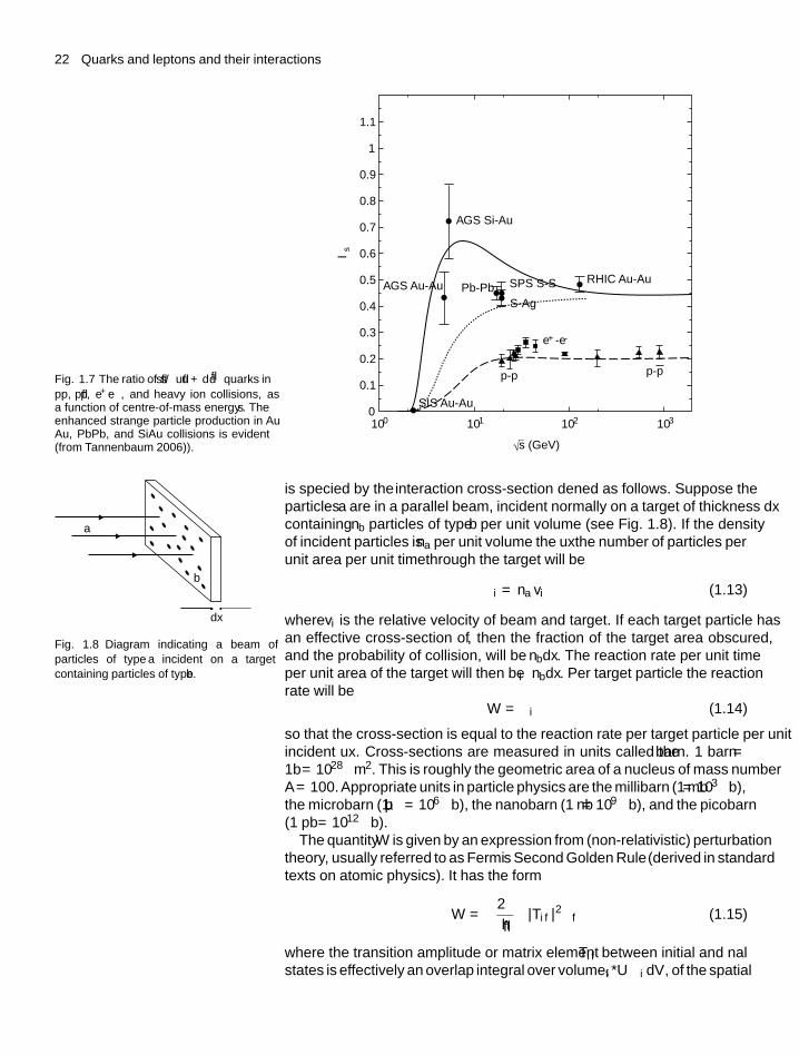
Figure 1.7 shows the results of a compilation of data on the ratio of strange tonon-strange particles as a function of centre-of-mass energy, from a review byTannenbaum (2006). It is not clear at present whether the differences observedbetween nucleus–nucleus and nucleon–nucleon or electron–positron collisionsare in fact due to such a phase transition. Obviously, present and future studiesof such plasma effects in the laboratory (specifically at the RHIC heavy ioncollider at Brookhaven National Laboratory, and the Large Hadron Collider atCERN), could be very important in shedding light on exactly how the earlyuniverse evolved.
1.8 The interaction cross section
The strength of the interaction between two particles, for example, in the two-body → two-body reaction
a + b → c + d
22 Quarks and leptons and their interactions
Fig. 1.7 The ratio of ss/(uu + dd
)quarks in
pp, pp, e+e−, and heavy ion collisions, asa function of centre-of-mass energy
√s. The
enhanced strange particle production in Au–Au, Pb–Pb, and Si–Au collisions is evident(from Tannenbaum 2006)).
AGS Si-Au
RHIC Au-Au
ls
p-pp-p
100 101 102 103
SPS S-SPb-PbS-Ag
AGS Au-Au
SIS Au-Au
e+ -e-
s (GeV)
1.1
1
0.9
0.8
0.7
0.6
0.5
0.4
0.3
0.2
0.1
0
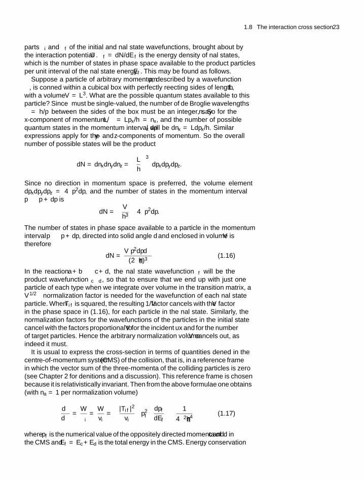
is specified by the interaction cross-section σ defined as follows. Suppose theparticles a are in a parallel beam, incident normally on a target of thickness dxcontaining nb particles of type b per unit volume (see Fig. 1.8). If the densityof incident particles is na per unit volume the flux—the number of particles perunit area per unit time—through the target will be
dx
a ��
b
Fig. 1.8 Diagram indicating a beam ofparticles of type a incident on a targetcontaining particles of type b.
φi = na vi (1.13)
where vi is the relative velocity of beam and target. If each target particle hasan effective cross-section of σ, then the fraction of the target area obscured,and the probability of collision, will be σnbdx. The reaction rate per unit timeper unit area of the target will then be φiσnbdx. Per target particle the reactionrate will be
W = φiσ (1.14)
so that the cross-section is equal to the reaction rate per target particle per unitincident flux. Cross-sections are measured in units called the barn. 1 barn =1b = 10−28 m2. This is roughly the geometric area of a nucleus of mass numberA = 100. Appropriate units in particle physics are the millibarn (1 mb = 10−3 b),the microbarn (1 μb = 10−6 b), the nanobarn (1 nb = 10−9 b), and the picobarn(1 pb = 10−12 b).
The quantity W is given by an expression from (non-relativistic) perturbationtheory, usually referred to as ‘Fermi’s Second Golden Rule’(derived in standardtexts on atomic physics). It has the form
W =(
2π
h
)|Ti f |2 ρf (1.15)
where the transition amplitude or matrix element Ti f between initial and finalstates is effectively an overlap integral over volume, ∫ψf *Uψi dV , of the spatial
1.8 The interaction cross section 23
parts ψi and ψf of the initial and final state wavefunctions, brought about bythe interaction potential U . ρf = dN/dEf is the energy density of final states,which is the number of states in phase space available to the product particlesper unit interval of the final state energy Ef . This may be found as follows.
Suppose a particle of arbitrary momentum p, described by a wavefunctionψ, is confined within a cubical box with perfectly reflecting sides of length L,with a volume V = L3. What are the possible quantum states available to thisparticle? Since ψ must be single-valued, the number of de Broglie wavelengthsλ = h/p between the sides of the box must be an integer, say n. So for thex-component of momentum, L/λ = Lpx/h = nx, and the number of possiblequantum states in the momentum interval dpx will be dnx = Ldpx/h. Similarexpressions apply for the y- and z-components of momentum. So the overallnumber of possible states will be the product
dN = dnxdnydnz =(
L
h
)3
dpxdpydpz .
Since no direction in momentum space is preferred, the volume elementdpxdpydpz = 4πp2dp, and the number of states in the momentum intervalp → p + dp is
dN =(
V
h3
)4πp2dp.
The number of states in phase space available to a particle in the momentuminterval p → p + dp, directed into solid angle d� and enclosed in volume V istherefore
dN = V p2dpd�
(2πh)3(1.16)
In the reaction a + b → c + d, the final state wavefunction ψf will be theproduct wavefunction ψcψd , so that to ensure that we end up with just oneparticle of each type when we integrate over volume in the transition matrix, aV −1/2 normalization factor is needed for the wavefunction of each final stateparticle. When Ti f is squared, the resulting 1/V factor cancels with the V factorin the phase space in (1.16), for each particle in the final state. Similarly, thenormalization factors for the wavefunctions of the particles in the initial statecancel with the factors proportional to V for the incident flux and for the numberof target particles. Hence the arbitrary normalization volume V cancels out, asindeed it must.
It is usual to express the cross-section in terms of quantities defined in thecentre-of-momentum system (CMS) of the collision, that is, in a reference framein which the vector sum of the three-momenta of the colliding particles is zero(see Chapter 2 for definitions and a discussion). This reference frame is chosenbecause it is relativistically invariant. Then from the above formulae one obtains(with na = 1 per normalization volume)
dσ
d�= W
φi= W
vi=(
|Ti f |2vi
)p2
f
(dpf
dEf
)(1
4π2h4
)(1.17)
where pf is the numerical value of the oppositely directed momenta of c and d inthe CMS and Ef = Ec +Ed is the total energy in the CMS. Energy conservation
24 Quarks and leptons and their interactions
gives √p2
f + m2c +√
p2f + m2
d = Ef
and thusdpf
dEf= EcEd
Ef pf= 1
vf
where vf is the relative velocity of c and d . Then
dσ
d�(a + b → c + d) = 1
4π2h4|Ti f |2
p2f
vi vf(1.18)
We have so far neglected the spins sa, sb, sc, and sd of the particles involved.If a and b are unpolarized, that is, their spin substates are chosen at random,the number of possible substates for the final state particles is gf = (2sc + 1)(2sd+1) and the cross-section has to include the factor gf . For the initial state thefactor is gi = (2sa +1) (2sb + 1). Since a given reaction has to proceed througha particular spin configuration, one must average the transition probability overall possible initial states, all equally probable, and sum over all final states. Thisimplies that the cross-section has to be multiplied by the factor gf /gi.
The reduction in the number of incident particles n = na after passage througha thickness dx of absorber in Fig. 1.8 is
dn = −nσρ dx
where ρ = nb is the density of target particles. Integrating we obtain
n(x) = n(0) exp(−σρx) (1.19)
Thus the proportion of incident particles which survive without interaction fallsto 1/e in a distance
λ = 1
(σρ)(1.20)
The quantity λ is called the mean free path for interaction. It is left as an exerciseto show that, from the distribution (1.19) and the definition (1.20), λ is the meanpath length between collisions.
1.9 Examples of elementary particlecross sections
The two-body to two-body reactions described above are important indiscussing the role of elementary particle interactions in the early universe,and we give here some examples. A full evaluation of the cross-sections wouldin some cases involve rather lengthy Dirac algebra, so that all that we shalldo here is to give approximate expressions which can be justified simply ondimensional grounds, and which will give orientation on the dependencies andmagnitudes involved. For simplicity we also neglect considerations of spin atthis stage. Spin and helicity factors are taken into account later in the text, whenexact cross-sections are required.
1.9 Examples of elementary particle cross sections 25
As (1.18) indicates, the differential cross-section for an extreme relativistictwo-body to two-body elastic collision has the form, in units h = c = 1
dσ
d�= |Tif |2 s
64π2
(extreme relativistic two-body → two-body
)(1.21)
where s = E2f denotes the square of the CMS energy, and Ef = 2pf , since the
masses involved are small compared with the energies, and vi = vf = 2. Inthis case also, the four-momentum transfer squared is |q2| = 2p2
f (1 – cos θ)where θ is the angle of emission of the secondary particles in the CMS, so thatdq2 = p2
f d�/π and (1.21) can also be written:
dσ
dq2= |Tif |2
16π(1.22)
Examples of electromagnetic cross-sections are as follows:
(a) e−μ+ → e−μ+
This is an example of the Coulomb scattering between singly charged leptons,as shown in Fig. 1.9(a). The couplings and photon propagator term togethergive |Tif | = e2/
∣∣q2∣∣ so that
dσ
d�∼ α2s
q4(1.23)
where α = e2/4π. This is just the Rutherford formula for pointlike scattering,and if θ is the angular deflection of the incident particle, then q = 2p sin (θ/2)
and one obtains the famous cosec4 (θ/2) dependence on scattering angle
(b) e+e− → μ+μ−
The diagram for this process, in Fig. 1.9(b), is just that in (a) rotated through90◦ and with outgoing leptons replaced by incoming antileptons and vice-versa.These two diagrams are said to be ‘crossed’ diagrams. In this case |q2| = s, the
gg
e–
e+
e–
e+
g
Q
e
e*
g g
e
e*
g
ge–
e+
e*
g
g e–
e+
(f)
e
(e)
W ±
e–
e+
e–
e+
Z 0e W ±
t
+
e–
m+ m–
m+ Q
n
n
ne
nene
ene
(a)
(d)
(b) (c)
Fig. 1.9 Feynman diagrams for variouselementary two-body to two-body reactions.In these diagrams. Time flows from left toright. The convention is that right-pointingarrows denote particles, while left-pointingarrows denote antiparticles. Diagrams (a) to(d) refer to electromagnetic interactions, and(e) and (f) to weak interactions. (a) e−μ+ →e−μ+; (b) e+e− → μ+μ−; (c) e+e− →QQ → hadrons; (d) eγ → eγ , e+e− → γγ ,γγ → e+e−; (e) νe → νe; (f) e+e− → vv.
26 Quarks and leptons and their interactions
square of the CMS energy, so that
dσ
d�∼ α2
s(1.24)
In fact a full calculation gives for the total cross-section
σ = 4πα2
3s(1.25)
This is the cross-section based upon single photon exchange, as shown by thedashed line in Fig. 1.10. There will also be a contribution from Z0 exchange,but because of the propagator term in (1.9), this is strongly suppressed at GeVenergies. The above result is also expected on dimensional grounds. In unitsh = c = 1, the cross-section has dimensions of GeV−2 and if the CMS energydominates over the lepton masses involved, the 1/s dependence must follow.Since, from Table 1.1, 1 GeV−1 = 1.975 × 10⁻¹⁶ m, the above cross-sectionis readily calculated to be 87/s nb (with s in GeV2).
(c) e+e− → QQ → hadrons
The same formula (1.24) applies, again assuming the quarks have relativisticvelocities, replacing the unit charges by the fractional quark charges at theright-hand vertex (Fig. 1.9(c)), and multiplying by a factor 3 for the numberof quark colours. Of course one does not observe the actual quarks: they‘fragment’ into hadrons by gluon exchanges as shown, but this is a relativelyslow and independent second-stage process. Except near meson resonances,the cross-section is determined entirely by the elementary e+e− → QQprocess.
Figure 1.10 shows a plot of the cross-section as a function of energy. Thepeaks are due to the excitation of bound quark–antiquark states or resonancesforming short-lived mesons: for example, the ρ and ω-mesons formed fromu and d quarks and antiquarks; the φ formed from ss; the J/ψ formed fromcc, the ϒ from bb, and finally the Z0 resonance. Nevertheless, the general 1/sdependence of the cross-section, aside from these resonance effects, is quiteclear.
Example 1.3 Calculate the ratio R of the cross-section for e+e− →QQ → hadrons, to that for e+e− → μ+μ−, via photon exchange, asa function of CMS energy (see also Fig. 1.10).
The quark–antiquark cross-section is proportional to the square of thequark charges and carries a factor 3 for colour. Thus for uu, dd , and ssquarks, the factor is
R = 3 ×[(
2
3
)2
+(
1
3
)2]
= 2
and this is shown as the first ‘step’ above the pointlike cross-section for amuon pair in Fig. 1.10. Above the charmed (cc) threshold appears a secondstep with R = 11/3, and above the bb threshold at CMS energy of 10 GeV,R = 11/3.

1.9 Examples of elementary particle cross sections 27
ϒ,ϒ�
4pa2
3s87.0
s
�/� � J/�
��
Z 0
W+W–
�(point) =
= nb
10–32
10–34
10–36
10–38
10–30
1 10 102 103
√s= CMS energy (GeV)
Cro
ss s
ectio
n (c
m2 ) 1 nb
1 pb
�(e+e– → anything)
Fig. 1.10 The cross-section for the reactione+e− → anything, as a function of CMSenergy. The prominent peaks are due tovarious boson resonances, as described in thetext. The overall 1/s dependence, typical ofa pointlike scattering process, is clear. Themagnitude of the cross-section for e+e− →anything, compared with that for muon pairproduction, shown as a dashed line, providesevidence for a factor 3 for the hadroniccross-section due to the colour degree offreedom of the quarks. The data are taken frommeasurements at various electron–positroncolliders, the largest of which was the LEPcollider at CERN, Geneva, in which 100GeV electrons collided head-on with 100 GeVpositrons.
Example 1.4 Estimate an approximate value for the cross-section for theproduction of the top quark, of mass mt= 175 GeV/c2, in proton–antiprotoncollisions at centre-of-mass energies large compared with the quark mass.
The top quark was discovered in 1995 at the Fermilab proton–antiprotoncollider, with a collision energy of 1.8 TeV in the centre-of-mass system(CMS). The principal process is that of production of a tt pair in thecollision of a u or d quark from the proton with an antiquark from theantiproton, via gluon exchange, that is, u + u → t + t, as in Fig. 1.9(c)but with incident e+e− replaced by uu (or dd) and gluon exchange withcoupling αs replacing photon exchange with coupling α. Then from (1.24)we expect the cross-section to be σ ∼ Fα2
s /s, where s ∼ (2mt)2, that is,
assuming an incident QQ centre-of-mass energy just above threshold, withF representing the probability that the colliding quarks are above threshold.If we set αs = 0.1 as a typical value, mt = 175 GeV, then σ ∼ 30F pb. Thevalue of F depends on the momentum distribution of quarks in the nucleon.A detailed calculation ends up with a cross-section of 7 pb, in agreementwith observation.
Since the total proton–antiproton collision cross-section at these energiesis 80 mb, this meant that the top quark was produced in only about 1 in1010 collisions. Despite this huge background, top quarks could be detectedbecause of the very distinguishing features of their decays, for examplet → W + +b and t → W − + b. The W -bosons decay to give muons at wideangle and neutrinos, which manifest themselves as ‘missing’ energy andmomentum, while the b quarks produce hadronic jets, slightly displaced

28 Quarks and leptons and their interactions
from the main vertex because of the finite lifetime of the B-mesons. Thesignal is so characteristic and specific that the background could be reducedbelow the 10% level. One of the detectors used in discovering the top quarkis shown in Fig. 1.11.
(d) e+e− → γ γ , γ γ → e+e−, γ e → γ e
These are important processes in astrophysics. They can all be represented bythe same Feynman diagram, as in Fig. 1.9(d). Because in this case a virtualelectron, rather than photon, operates between the vertices, the formula (1.24)is modified by a logarithmic term. Of course, although represented by the samediagram, the three processes have different dynamics (thresholds). In the limitof high energy, that is, for CMS energy squared s � m2 where m is the electronmass, the cross-sections have the asymptotic forms:
σ(e+e− → γγ
) =(
2πα2
s
)[ln( s
m2
)− 1]
(1.26a)
σ(γγ → e+e−) =
(4πα2
s
)[ln( s
m2
)− 1]
(1.26b)
σ (γe → γe) =(
2πα2
s
)[ln( s
m2
)+ 1
2
](1.26c)
Fig. 1.11 Photograph of the CDF detectoremployed in the discovery of the top quarkin 1995, in collisions of 0.9 TeV protons with0.9 TeV antiprotons at the proton–antiprotoncollider at Fermilab, near Chicago. In thecentre of the picture is the central trackingdetector, which records the trajectoriesof individual secondary particles in driftchambers, and measures their momenta fromtrack curvature in the applied magnetic field.Inside this are precision solid-state (siliconstrip) detectors which can record tracks andsecondary vertices very close to the maininteraction vertex. Surrounding the centraltracker are calorimeters which measure thetotal energy in charged and neutral particles.They are built in two arches which arewithdrawn in the photograph. Outside thecalorimeter modules and magnet yoke arefurther chambers to record penetrating muonsfrom the annihilation reactions. (CourtesyFermilab Visual Media Services).
1.9 Examples of elementary particle cross sections 29
The fact that the cross-section (1.26a) is half that of (1.26b) arises because inthe first process there are two indistinguishable particles in the final state, sothat the phase–space volume is halved. At collision energies large comparedwith the W mass, a formula similar to (1.26a) would apply to the reactione+e− → W +W −. The last process (1.26c) is known as Compton scattering.The same formula applies when the roles of incident and target particle arereversed, that is, γ-rays are accelerated to higher energies following collisionwith incident electrons. This inverse Compton effect is believed to be importantin the production of high-energy γ-rays from point stellar sources.
At the other extreme of low CMS energy, the electron mass will dominate theenergy scale and s is replaced by m2, so that σ ∼ α2/m2. In fact the classicalThomson cross-section, applying for Compton scattering as Eγ → 0, has thevalue
σ (γe → γe)Thomson = 8πα2
3m2= 0.666 barns (1.26d)
For the process γγ → e+e−, the threshold energy is sth = 4m2 and σ ∼ βα2/s,
where β = (1 − 4m2/s)1/2
is the CMS velocity of the electron or positron.Thus the cross-section at first increases with energy, and reaches a maximumof about 0.25σThomson at s ∼ 8m2, before falling off at higher s values.
In summary, the above processes involve massless or almost massless photonor electron propagators and their effect is to introduce a 1/s dependence to thecross-sections. We now discuss weak processes which involve the massive Wand Z propagators.
(e) vee → vee; e+e− → veve
Figure 1.9(e) shows the diagram for neutrino–electron scattering viaW−exchange. There is also a contribution from Z exchange, but we considerhere only the former. The propagator gives a term 1/
(∣∣q2∣∣+ M 2
W
)in |Tif |.
Because of the large value of the W mass (80 GeV), |q2| M 2W at normal (<1
TeV) neutrino energies and therefore
σ ∼ g4ws
M 4W
∼ G2Fs (1.27a)
where GF is the Fermi constant defined in (1.9). An exact calculation gives
σ (vee → vee) = G2Fs
π(1.27b)
again assuming that lepton masses can be neglected in comparison with thecollision energy. For the ‘crossed’ reaction e+e− → veve shown in Fig. 1.9(f),the cross-section is (see Section 3.6):
σ(e+e− → veve
) = G2Fs
6π(1.28)
In addition to W ± exchange, this reaction can also proceed through Z0
exchange, and indeed this is the only possibility for the reactions e+e− → vμvμ
30 Quarks and leptons and their interactions
or vτ vτ . These processes are also discussed in Section 3.6. They are ofastrophysical significance, both in the very early stages of the universe, andin the later supernova stages of giant stars.
1.10 Decays and resonances
As indicated in (1.15), an unstable state has a decay rate W , usually quoted asa width � in energy units, which corresponds to the fact that a non-stationarystate with a finite lifetime must have a spread in energy, in accord with theuncertainty relation, that is � = hW = h/τ where τ = 1/W is the meanlifetime of the state.
As an example of a decaying state, let us consider muon decay, μ+ →e+ + ve + vμ. Clearly the transition amplitude for this weak decay |Ti f | ∝ GF,the Fermi coupling constant, which has dimensions (energy)−2—see Table 1.5.Hence the square of the transition amplitude has dimensions (energy)−4 whilethe decay rate or width has dimensions of energy. Thus by dimensionalarguments the phase–space factor in (1.15) must vary as (energy)5, and sincethe largest energy or mass involved is mμc2 it follows that the muon decay rate� ∼ G2
Fm5μ. In fact a full (and quite lengthy) calculation gives
�(μ+ → e+vevμ
) = G2Fm5
μ
192π3(1.29)
It is left as an exercise to verify the value of the Fermi constant in Table 1.5from the measured lifetime τμ = h/� = 2.197 μs and mass mμc2 = 105.66MeV (one should remark that the result will not be quite exact, because thereare radiative corrections at the per cent level).
One can understand that a state with a measurable lifetime usually has anunmeasurably small width, while one with a broad and measurable width,for example, one decaying through the strong interactions, usually has anunmeasurably short lifetime, and is referred to as a resonance. Such resonancescan readily be formed in collisions between the particles into which they decay.The exponential nature of the time distribution of decays determines the formof the line shape of the resonance.
Denoting the central frequency of the resonant state by ωR, the wavefunctiondescribing this state can be written
ψ (t) = ψ(0) exp (−iωRt) exp
(− t
2τ
)= ψ(0) exp
{−t(iER + (�/2
))h
}(1.30)
where the central energy is ER = hωR and the width � = h/τ. The intensityI(t) = ψ∗(t) ψ(t) obeys the usual radioactive decay law
I(t)
I(0)= exp
(−�t
h
)(1.31)
The energy dependence of the cross-section for forming the resonance is theFourier transform of the time pulse, in the same way that, in wave optics,
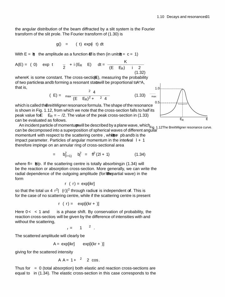
1.10 Decays and resonances 31
the angular distribution of the beam diffracted by a slit system is the Fouriertransform of the slit profile. The Fourier transform of (1.30) is
g(ω) =∫
ψ(t) exp(iωt) dt
With E = hω the amplitude as a function of E is then (in units h = c = 1)
A(E) = ψ(0)
∫exp
{−t
[(�
2
)+ i (ER − E)
]}dt = K{
(E − ER) − (i�/2)}
(1.32)where K is some constant. The cross-section σ(E), measuring the probabilityof two particles a and b forming a resonant state c will be proportional to A*A,that is,
σ(E) = σmax�2/
4[(E − ER)2 + (�2
/4)] (1.33)
which is called the Breit–Wigner resonance formula. The shape of the resonanceis shown in Fig. 1.12, from which we note that the cross-section falls to half itspeak value for E − ER = ±�/2. The value of the peak cross-section in (1.33)can be evaluated as follows.
Γ
1.0
0.5
ER E
�max
�
Fig. 1.12 The Breit–Wigner resonance curve.An incident particle of momentum p will be described by a plane wave, whichcan be decomposed into a superposition of spherical waves of different angularmomentum l with respect to the scattering centre , where lh = pb and b is the‘impact parameter’. Particles of angular momentum in the interval l → l + 1therefore impinge on an annular ring of cross-sectional area
σ = π(
b2(l+1) − b2
l
)= πλ2 (2l + 1) (1.34)
where λ = h/p. If the scattering centre is totally absorbing, σ in (1.34) willbe the reaction or absorption cross-section. More generally, we can write theradial dependence of the outgoing amplitude (for the lth partial wave) in theform
r ψ(r) = exp[ikr]so that the total flux 4πr2|ψ(r)|2 through radius r is independent of r. This isfor the case of no scattering centre, while if the scattering centre is present
r ψ(r) = η exp[i(kr + δ)]Here 0 < η < 1 and δ is a phase shift. By conservation of probability, thereaction cross-section σr will be given by the difference of intensities with andwithout the scattering,
σr = σ(
1 − η2)
.
The scattered amplitude will clearly be
A = exp[ikr] − η exp[i(kr + δ)]giving for the scattered intensity
A∗A = 1 + η2 − 2η cos δ.
Thus for η = 0 (total absorption) both elastic and reaction cross-sections areequal to σ in (1.34). The elastic cross-section in this case corresponds to the
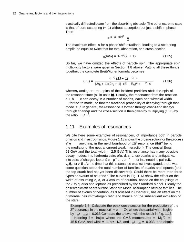
32 Quarks and leptons and their interactions
elastically diffracted beam from the absorbing obstacle. The other extreme caseis that of pure scattering (η = 1) without absorption but just a shift in phase.Then
σel = 4σ sin2(
δ
2
)The maximum effect is for a phase shift of π radians, leading to a scatteringamplitude equal to twice that for total absorption, or a cross-section
σel(max) = 4πλ2(2l + 1) (1.35)
So far, we have omitted the effects of particle spin. The appropriate spinmultiplicity factors were given in Section 1.8 above. Putting all these thingstogether, the complete Breit–Wigner formula becomes
σ(E) = 4πλ2 (2J + 1)(�2/
4)
(2sa + 1) (2sb + 1)[(E − ER)2 + (�2
/4)] (1.36)
where sa and sb are the spins of the incident particles and J is the spin ofthe resonant state (all in units of h). Usually, the resonance from the reactiona + b → c can decay in a number of modes, each one with a partial width�i for the ith mode, so that the fractional probability of decaying through thatmode is �i/�. In general, the resonance is formed through channel i and decaysthrough channel j, and the cross-section is then given by multiplying (1.36) bythe ratio �i�j/�
2.
1.11 Examples of resonances
We cite here some examples of resonances, of importance both in particlephysics and in astrophysics. Figure 1.13 shows the cross-section for the processe+e− → anything, in the neighbourhood of the Z0 resonance (the Z0 beingthe mediator of the neutral current weak interaction). The central mass ER =91 GeV and the total width � = 2.5 GeV. This resonance has many possibledecay modes; into hadrons via pairs of u, d, s, c, or b quarks and antiquarks,into pairs of charged leptons e+e−, μ+μ−, or τ+τ−, or into neutrino pairs veve,vμvμ, or vτ vτ . At the time that this resonance was first investigated, there wassome question about the total number of families of quarks and leptons (andthe top quark had not yet been discovered). Could there be more than threetypes or flavours of neutrino? The curves in Fig. 1.13 show the effect on thewidth of assuming 2, 3, or 4 flavours of neutrino, based on the couplings ofthe Z to quarks and leptons as prescribed by the Standard Model. Clearly theobserved width bears out the Standard Model assumption of three families. Thenumber of flavours of neutrino, as discussed in Chapter 6, has an effect on theprimordial helium/hydrogen ratio and thence on the subsequent evolution ofthe stars.
Example 1.5 Calculate the peak cross-section for the production of theZ0resonance in the reaction e+ + e−→ Z0, where the partial width is givenby �ee/�total = 0.033. Compare the answer with the result in Fig. 1.13.
Inserting λ = hc/pc where the CMS momentum pc = MZ/2 =45.5 GeV, and with J = 1, s = 1/2, and �ee/�tot = 0.033, one obtains
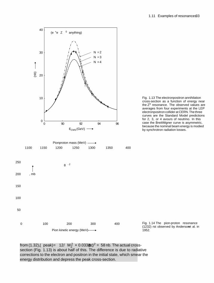
1.11 Examples of resonances 33
0 90 92 94 96
�(e+e– → Z 0 → anything)
ECMS (GeV)
� (n
b)
Nν = 2
Nν = 3
Nν = 4
40
30
20
10
0
Fig. 1.13 The electron–positron annihilationcross-section as a function of energy nearthe Z0 resonance. The observed values areaverages from four experiments at the LEPelectron–positron collider at CERN. The threecurves are the Standard Model predictionsfor 2, 3, or 4 flavours of neutrino. In thiscase the Breit–Wigner curve is asymmetric,because the nominal beam energy is modifiedby synchrotron radiation losses.
250
200
150
100
50
0 100 200
Pion kinetic energy (MeV)
300 400
1100 1150 1200 1250 1300 1350 400
�, mb
8πλ2
Pion–proton mass (MeV)
Fig. 1.14 The pion-proton resonance �
(1232) first observed by Anderson et al. in1952.
from (1.32), σ(peak) = [12π/M 2Z
]×0.033(hc)2 = 58 nb. The actual cross-section (Fig. 1.13) is about half of this. The difference is due to radiativecorrections to the electron and positron in the initial state, which smear theenergy distribution and depress the peak cross-section.
34 Quarks and leptons and their interactions
Figure 1.14 shows the first resonance ever to be discovered in high-energyphysics, namely the �(1232) pion-proton resonance observed in 1952. It hascentral mass 1232 MeV/c2 and width � = 120 MeV. This observation wasfollowed by that of many other meson–meson and meson–baryon resonancesin the 1950s and 1960s. These resonant states were important in providingthe essential clues which led to the development of the quark model by Gell-Mann and by Zweig in 1964. The � resonance is also of present astrophysicalsignificance in connection with the very highest-energy cosmic rays, since itcan be excited in collisions of protons above 1019 eV energy with the cosmicmicrowave background, with quantum energy of order of 0.25 meV (milli-electron volt). Known as the GZK effect after Greisen, Zatsepin, and Kuzminwho suggested it, the resonance indeed leads to a cut off in the cosmic rayspectrum above 1019 eV (see Section 9.12).
From the viewpoint of the human race, possibly the most important resonanceis that of the 0+ excited state of the 12C nucleus at an excitation energy of 7.654MeV. The width is about 10 eV only. The production of carbon in helium-burning red giant stars, discussed in Chapter 10, is achieved through the so-called triple alpha process, 3α → 12C. First, two alpha particles combine toform 8Be in its ground state, which is unstable with a lifetime of only 10−16
sec. It may nevertheless capture a third alpha particle to form carbon, which,however, usually decays back into beryllium plus an alpha particle, but canwith a small (10−3) probability decay by gamma emission to the ground stateof carbon. The rate of 12C production depends crucially on the existence of thisresonance level, occurring just 400 keV above the threshold energy, to enhancethe triple alpha cross-section. Indeed, Hoyle had predicted the need for such aresonance and its properties in 1953, before it was finally found in laboratoryexperiments. Without the existence of this resonance, it is almost certain thatcarbon-based biological evolution in the universe could never have taken place.
1.12 New particles
The Standard Model of the fundamental quarks and leptons and theirinteractions described here and in Chapter 3 is able to account for practicallyall laboratory experiments at accelerators to date, and describes with greataccuracy the physics of the fundamental particles, at least in our particularcorner of the universe. However, it apparently does not describe the buildingblocks of the universe on large scales. Indeed on such scales it can accountfor only about 4% of the total energy density! As described in Chapter 7,study of the kinematics of large-scale cosmic structures—galaxies, galaxyclusters, and superclusters—indicates that the bulk of the matter in the universeis invisible (i.e. non-luminous) dark matter. The nature of this dark matter ispresently unknown. There is so far no direct experimental evidence for detectionof individual dark matter particles. It is possible that the proposed massivesupersymmetric particles mentioned in Section 1.3 could be candidates.
Present experiments in astrophysics, to be described in the followingchapters, also indicate that, although in the past the universal expansionfollowing the Big Bang was indeed slowing down (on account of the restrainingpull of gravity), the expansion is now accelerating, this being ascribed to dark
1.13 Summary 35
energy which actually exerts a gravitational repulsion. This dark energy exceedsthe energy density in all other matter and radiation. Again, the actual natureand origin of this dark energy is presently unknown.
The possibilities of new particles and new interactions also follow from thevery successes of the Standard Model, in being able to unify electromagneticwith weak interactions in the electroweak theory. This suggests that it might alsobe possible to unify strong with electroweak interactions in a so-called grandunified theory (GUT). At present, however, there is no direct experimentalsupport for such higher levels of unification. The reasons for these schemes,and their consequences for the experimental situation are discussed in Chapters3 and 4. The evidence for higher mass scales, well above anything attainablein the laboratory, may also be suggested by the success of inflationary modelsof the early universe, described in Chapter 8, and by the evidence for finiteneutrino masses, described in Chapters 4 and 9.
Even more ambitious than the proposed unification of strong, weak,and electromagnetic interactions, is the attempt to unify all fundamentalinteractions, including gravity, in so-called superstring theory (see Chapter 3).This can produce a unified, renormalizable quantum theory of the fundamentalinteractions, but only in 10-dimensional space–time (for fermions). One mustsuppose that all but the normal four dimensions of space and time are ‘curled up’to the tiny dimensions of the Planck length (1.12), according to ideas originallyadvanced by Kaluza and Klein in the 1920s. Unfortunately, apart from thesingle prediction of spin 2 for the graviton, superstring theories appear so farto make no testable predictions.
1.13 Summary
• Matter is built from elementary fermion constituents, the quarks andleptons, occurring in three ‘families’. Each family consists of a quarkwith charge +2|e|/3 and one of −|e|/3, a charged lepton with charge−|e|, and a neutral lepton (neutrino). The antiparticles of these stateshave electric charges of opposite sign but are otherwise identical to theparticles.
• The observed strongly interacting particles (hadrons) consist of boundquark combinations. Baryons consist of three quarks and mesons of aquark–antiquark pair.
• Quarks and leptons interact via exchange of fundamental bosons,characteristic of four fundamental interactions: strong, electromagnetic,weak, and gravitational. The exchanged bosons are virtual particles.
• Strong interactions occur between quarks and are mediated by gluonexchange; electromagnetic interactions are between all charged particlesand are mediated by photon exchange; weak interactions are mediated byW ± and Z0 exchange; gravitational interactions via graviton exchange.Photons, gluons, and gravitons are massless. W and Z bosons havemasses of 80 and 91 GeV/c2 respectively.
• The basic boson exchange process can be visualized by diagrams calledFeynman diagrams, depicting the exchange of a virtual boson betweentwo interacting fermions. The amplitude for this process is the productof the couplings g1 and g2 of the fermions to the exchanged boson,
36 Quarks and leptons and their interactions
multiplied by a propagator term which depends on the (free) bosonmass M and the momentum transfer q, of the form 1/
(M 2 − q2
), where
q2 is a negative quantity. The cross-section for the interaction is theproduct of the square of the above amplitude and a phase–space factor.It is numerically equal to the reaction rate per target particle per unitincident flux.
• The strength of an interaction is also measured by the decay rate or widthof unstable hadronic or leptonic states. If the width is large enough to bemeasurable, the state is referred to as a resonance.
• Under normal conditions, quarks are confined as combinations in baryons(QQQ) or mesons (QQ). At sufficiently high temperatures, with kT > 0.3GeV, it is expected that quarks would no longer be confined, and thathadrons would undergo a phase transition to a quark–gluon plasma.
Problems
A table of physical constants can be found in Appendix A.More challenging problems are marked with an asterisk.
(1.1) Find the fractional change in total energy (includingrest energy and gravitational potential energy) whentwo equal and isolated point masses M are broughtfrom infinity to a separation R. Calculate what this iswhen (a) M equals one solar mass and R equals 1 parsecand (b) when M equals the Planck mass and R equals1 fm.
*(1.2) The bombardment of a proton target by a pion beam ofenergy 1 GeV/c results in the reactionπ−+p → �+K0
with a cross-section of about 1 mb. The K0 particle is ameson of strangeness S = +1, while the � is a baryonof strangeness S = −1. Write down the above reactionin terms of quark constituents.
Both of the product particles are unstable. Oneundergoes decay in the mode � → p + π− with amean lifetime of 10−10 s, while the other decays inthe mode K0 → π+ + π−, also with a lifetime of10−10 s. Both decay rates and interaction cross-sectionsare proportional to the squares of the coupling constantsassociated with the interactions responsible. Explainqualitatively how the long lifetimes for the abovedecays can be reconciled with the large productioncross-section. (Note: this contrast between the strongproduction cross-section and long decay lifetime wasthe reason for calling the � and K0 ‘strange’particles.)
(1.3) Calculate the energy carried off by the neutrino in thedecay of a pion at rest, π+ → μ+ + νμ. The relevantmasses are mπc2 = 139 MeV, mμc2 = 106 MeV,
mν ∼ 0. Pions in a beam of energy 10 GeV decayin flight. What is the maximum and minimum energiesof the muons from these decays? (See Chapter 2 forformulae on relativistic transformations.)
(1.4) The �++ resonance shown in Fig. 1.14 has a full widthof � = 120 MeV. What is the mean proper lifetime ofthis state? How far on average would such a particle,of energy 100 GeV, travel before decaying?
(1.5) The �− is a baryon of mass 1672 MeV/c2 andstrangeness S = −3. It decays principally to a �
baryon of mass 1116 MeV/c2 and S = −1 and a K−meson of mass 450 MeV/c2 and S = −1. Expressthe decay process in terms of quark constituents in aFeynman diagram.
State which of the following decay modes are possiblefor the � particle:
(a) �− → �0 +π− (m� = 1315 MeV/c2, S = −2)(b) �− → �− + π0 (m� = 1197 MeV/c2, S = −1)(c) �− → �0 + π− (m� = 1116 MeV/c2, S = −1)(d) �− → �+ + K− + K− (mK = 494 MeV/c2)
*(1.6) The following decays are all ascribed to the weakinteraction, resulting in three final state particles. Foreach process, the available energy Q in the decay isgiven together with the decay rate W :
(a) τ+ → e+ + ve + vτ
Q = 1775 MeVW = 6.1 × 10¹¹s−1
Problems 37
(b) μ+ → e+ + ve + vμ
Q = 105 MeVW = 4.6 × 10⁵ s−1
(c) π+ → π0 + e+ + νe
Q = 4.1 MeVW = 0.39 s−1
(d) 14O →14N* + e+ + νe
Q = 1.8 MeVW = 5.1 × 10⁻³ s−1
(e) n → p + e− + νe
Q = 0.78 MeVW = 1.13 × 10⁻³ s−1
Using dimensional analysis show that within one or twoorders of magnitude, the Q values and decay rates arecompatible with the same weak coupling. Comment onany trends with the values of Q.
*(1.7) The cross-section for neutrino–electron scatteringvia W−exchange is given in (1.27b) asσ (ve + e → ve + e) = G2
Fs/π, where s is thesquare of the CMS energy. At high energies, deepinelastic neutrino–nucleon scattering can be treated aselastic scattering of a neutrino by a quasi-free quarkconstituent of the nucleon, the scattered quark then‘fragmenting’ into secondary hadrons. Assuming thatthe struck quark carries on average 25% of the massof the nucleon, calculate the neutrino–nucleon cross-section in cm2 as a function of the laboratory neutrinoenergy in GeV.
*(1.8) In the previous question, the cross-section formulaassumes a pointlike interaction specified by the Fermiconstant GF. However at very high energies, the effectof the finite W boson mass in the propagator term(1.9) must be taken into account. Write down anexpression for the differential cross-section dσ/dq2
for neutrino–electron scattering in this case, based onEquation (1.27b) and the fact that the maximum valueof momentum transfer squared is q2(max) = s. Showthat, as q2(max) → ∞, the neutrino–electron cross-section tends to a constant, and find its value. At whatneutrino energy does the cross-section reach half of itsasymptotic value?
(1.9) A resonance of significance for experiments on ultra-high-energy neutrinos in astrophysics is the Glashowresonance:
ve + e− → W −
where MW c2 = 81 GeV. Assuming that the targetelectrons in the cosmos are at rest, show that thisresonance would be excited for antineutrino energiesof around 6400 TeV, and that the peak cross-sectionwould be about 5μb.
(1.10) The charmed meson D+ (mass 1.87 GeV/c2) undergoesweak �C = 1 decay in the mode D+ → K0 + l+ + νl
where l = e or μ, with a 15% branching ratio. Thequark constitution of the charmed meson is D+ = cdand of the kaon is K0 = sd , so the decay can be writtenas the transformation of a charmed to a strange quark(with a d -quark as ‘spectator’):
c → s + l+ + vl
in close analogy with muon decay. Draw the Feynmandiagram for c quark decay, and assuming a mass of thec quark of 1.6 GeV/c2, and neglecting the mass of thedecay products, estimate the lifetime of the D mesonfrom that of the muon as given in Problem 1.6.
(1.11) The �-baryons are combinations of s, u, and d quarks,with strangeness S = −1. The first two entries inthe Table on the next page are for the ground-statecombination of spin J = 1/2 while the third isan excited state of J = 3/2. The rest-masses inMeV/c2 are given in brackets, followed by the quarkconstitution, the Q−value, principal decay mode andlifetime or width. All the decay products have S = 0except for the �-baryon, which has S = −1.
State which of the fundamental interactions areresponsible for the above decays, and from the decayrates estimate the relative values of their couplingstrengths.
(1.12) Draw the Feynman diagram representing electron–electron scattering to first order in the couplingconstant. If you carefully label the incoming andoutgoing electron states, in fact you will find thattwo diagrams are possible. Draw some second-orderdiagrams involving exchanges of photons and/orelectron–positron pairs. Compare the interaction rateswith those for the first-order process.
(1.13) The following transitions have Q values and meanlifetimes as indicated:
Transition Q-value (MeV) Lifetime (s)(a) μ+ → e+ + ve + vμ 105 2.2 × 10⁻⁶
(b) μ− +12 C →12 B + νμ 93 2 × 10⁻⁶
(c) π0 → 2γ 135 10−17
(d) �++ → p + π+ 120 10−23
State which interactions are responsible in each case,and estimate the relative coupling strengths from thegiven quantities.
*(1.14) Calculate the ratio R of the cross-section for e+e− →QQ → hadrons to that for the reaction e+e− → μ+μ−in (1.25), as a function of increasing CMS energy up to20 GeV. Assume the quark masses given in Table 1.4.
At a certain energy, the process e+e− → π+ + π− +π0 is observed. Draw a Feynman diagram to illustratesuch an event.
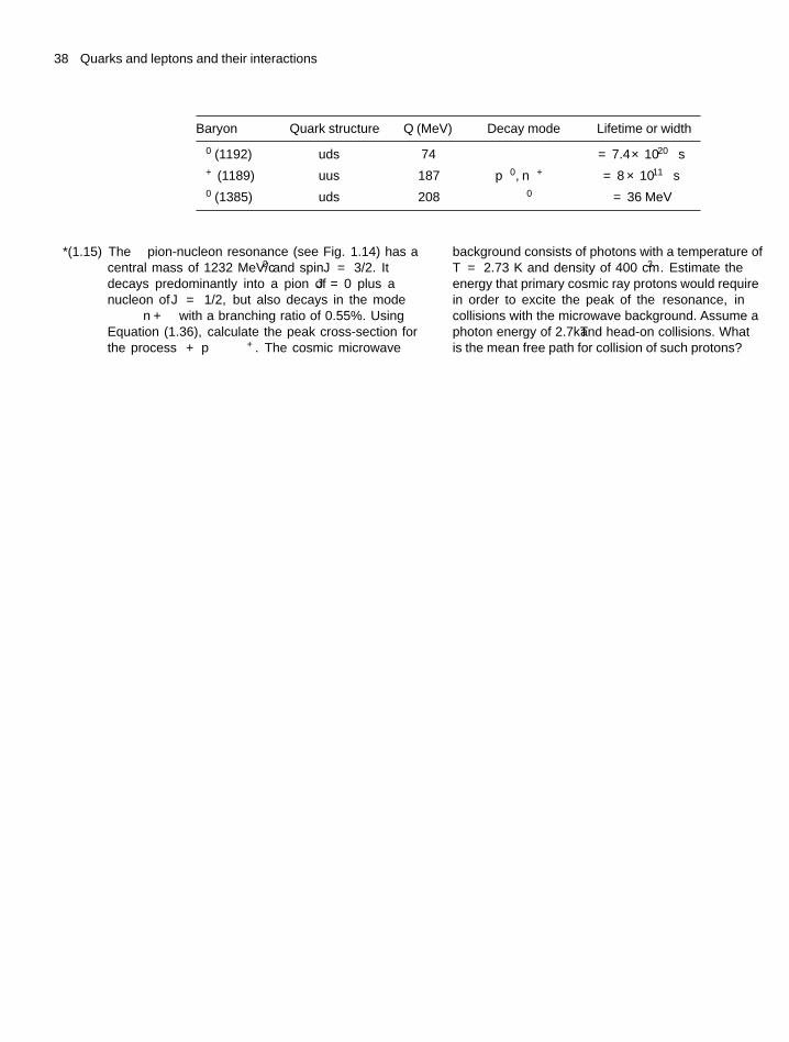
38 Quarks and leptons and their interactions
Baryon Quark structure Q (MeV) Decay mode Lifetime or width
�0 (1192) uds 74 �γ τ = 7.4 × 10⁻²⁰ s
�+ (1189) uus 187 pπ0, nπ+ τ = 8 × 10⁻¹¹ s
�0 (1385) uds 208 �π0 � = 36 MeV
*(1.15) The � pion-nucleon resonance (see Fig. 1.14) has acentral mass of 1232 MeV/c2 and spin J = 3/2. Itdecays predominantly into a pion of J = 0 plus anucleon of J = 1/2, but also decays in the mode� → n + γ with a branching ratio of 0.55%. UsingEquation (1.36), calculate the peak cross-section forthe process γ + p → �+. The cosmic microwave
background consists of photons with a temperature ofT = 2.73 K and density of 400 cm−3. Estimate theenergy that primary cosmic ray protons would requirein order to excite the peak of the � resonance, incollisions with the microwave background. Assume aphoton energy of 2.7kT and head-on collisions. Whatis the mean free path for collision of such protons?
Relativistictransformationsand the equivalenceprinciple
2As a precursor of a discussion of invariance principles and symmetries inChapter 3, we summarize in this chapter relativistic transformations and Lorentzinvariance, the Equivalence Principle, and important solutions of the Einsteinfield equations of general relativity. These are central to our discussions ofcosmology in later chapters. Readers familiar with these topics can skip toChapter 3.
2.1 Coordinate transformations inspecial relativity
The special theory of relativity, proposed by Einstein in 1905, involvestransformations between inertial frames (IFs) of reference. An IF is one inwhich Newton’s law of inertia holds: a body in such a frame not acted on byany external force continues in its state of rest or of uniform motion in a straightline. Although an IF is, strictly speaking, an idealized concept, a referenceframe far removed from any fields or gravitating masses approximates to sucha frame, as does a lift in free fall on Earth. On the scale of experiments inhigh-energy physics at accelerators, gravitational effects are negligibly smalland to all intents and purposes the laboratory can be treated as an IF. However,on the scale of the cosmos, gravity is the most important of the fundamentalinteractions.
We list here the coordinate transformations, called Lorentz transformations,among IFs in special relativity. These are obtained from two assumptions: thatthe coordinate transformations should be linear (to agree with the Galileantransformations in the non-relativistic limit); and that the velocity of light c invacuum should be the same in all IFs (as observed in numerous experiments).The relation between the coordinates x′, y′, z′, t′ of an event in an IF �′ movingwith velocity v along the x-axis with respect to an IF �, where the coordinatesof the event are x, y, z, and t, is then as follows:
x′ = γ (x − vt) y′ = y z′ = z t′ = γ(
t − vx
c2
)(2.1)
where γ = (1 − v2/c2)−1/2
is the so-called Lorentz factor. When v → 0, γ →1, x′ → (x − vt), and t′ → t as in the Galilean transformation. The above
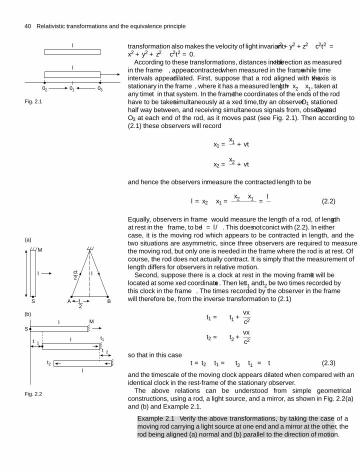
40 Relativistic transformations and the equivalence principle
transformation also makes the velocity of light invariant: x′2+y′2+z′2−c2t′2 =x2 + y2 + z2 − c2t2 = 0.
l�
l
02 0301
Fig. 2.1
According to these transformations, distances in the x-direction as measuredin the frame �′, appear contracted when measured in the frame �, while timeintervals appear dilated. First, suppose that a rod aligned with the x-axis isstationary in the frame �′, where it has a measured length l′ = x′
2 −x′1, taken at
any time t′ in that system. In the frame �, the coordinates of the ends of the rodhave to be taken simultaneously at a fixed time t, by an observer O1 stationedhalf way between, and receiving simultaneous signals from, observers O2 andO3 at each end of the rod, as it moves past (see Fig. 2.1). Then according to(2.1) these observers will record
x1 = x′1
γ+ vt
x2 = x′2
γ+ vt
and hence the observers in � measure the ‘contracted’ length to be
l = x2 − x1 =(x′
2 − x′1
)γ
= l′
γ(2.2)
Equally, observers in frame �′ would measure the length of a rod, of length xat rest in the � frame, to be l′ = l/γ . This does not conflict with (2.2). In eithercase, it is the moving rod which appears to be contracted in length, and thetwo situations are asymmetric, since three observers are required to measurethe moving rod, but only one is needed in the frame where the rod is at rest. Ofcourse, the rod does not actually contract. It is simply that the measurement oflength differs for observers in relative motion.
Second, suppose there is a clock at rest in the moving frame �′. It will belocated at some fixed coordinate x′. Then let t′1 and t′2 be two times recorded bythis clock in the frame �′. The times recorded by the observer in the frame �
will therefore be, from the inverse transformation to (2.1)
t1 = γ
(t′1 + vx′
c2
)t2 = γ
(t′2 + vx′
c2
)so that in this case
t = t2 − t1 = γ(t′2 − t′1
) = γt′ (2.3)
and the timescale of the moving clock appears dilated when compared with anidentical clock in the rest-frame of the stationary observer.
l� l
l
l
l
�
�t1
�t2
�
t2
t1
MS
M
ct
A
2
BS �t
(a)
(b)
2
Fig. 2.2 The above relations can be understood from simple geometricalconstructions, using a rod, a light source, and a mirror, as shown in Fig. 2.2(a)and (b) and Example 2.1.
Example 2.1 Verify the above transformations, by taking the case of amoving rod carrying a light source at one end and a mirror at the other, therod being aligned (a) normal and (b) parallel to the direction of motion.

2.2 Invariant intervals and four-vectors 41
Refer first to Fig. 2.2(a). The rod with a pulsed light source S at oneend and a mirror M at the other, is at rest and of length l′ in the �′ frame,which is moving at velocity v along the x-axis of the frame �, the rod beingaligned with the y-axis. The time for the light pulse to travel to the mirrorand back is clearly t′ = 2l′/c, as measured in the frame �′. However, in theframe �, the return journey time is t, during which time the rod has moveda distance vt along the x-axis. Since transverse distances are the same in thetwo frames (l = l′), the right-angled triangle gives(
ct
2
)2
=(
ct′
2
)2
+(
vt
2
)2
or t = t′√(1 − v2/c2
) = γt′ (2.4)
as before. In the second arrangement, in Fig. 2.2(b), the rod is aligned inthe x-direction. The time for the light pulse to travel to the mirror and backis again t′ = 2l′/c in the �′ frame. However, in the � frame the time t1 forthe pulse to reach the mirror is longer because the mirror has moved, and isgiven by ct1 = l + vt1, or t1 = l/(c − v). The return signal from the mirrorreaches the source after time t2, where ct2 = l − vt2, or t2 = l/(c + v).Hence the total time in the � system is
t = t1 + t2 = 2l
c(1 − v2/c2
) (2.5)
However, from (2.4) we know that
t = t′√(1 − v2/c2
) = 2l′
c√(
1 − v2/c2) (2.6)
Comparing the last two expressions we obtain the result (2.2) for theapparent contraction
l = l′
γ(2.7)
2.2 Invariant intervals and four-vectors
We have seen that the measured values of time and space intervals for the sameevent differ in different reference frames. However, the goal of relativity theoryis to formulate the equations of physics in a way that is invariant in all referenceframes. The invariant interval or line element is made up of the squares of thecoordinate differences for two events and is defined by
ds2 = c2dt′2 − dx′2 − dy′2 − dz′2
= c2dt2 − dx2 − dy2 − dz2 (2.8)
= c2dτ2
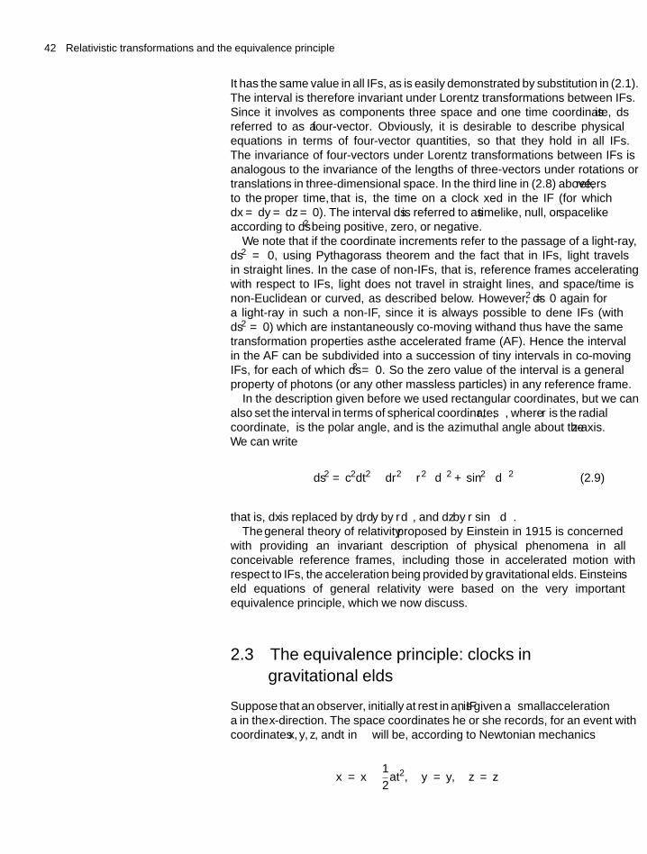
42 Relativistic transformations and the equivalence principle
It has the same value in all IFs, as is easily demonstrated by substitution in (2.1).The interval is therefore invariant under Lorentz transformations between IFs.Since it involves as components three space and one time coordinate, ds isreferred to as a four-vector. Obviously, it is desirable to describe physicalequations in terms of four-vector quantities, so that they hold in all IFs.The invariance of four-vectors under Lorentz transformations between IFs isanalogous to the invariance of the lengths of three-vectors under rotations ortranslations in three-dimensional space. In the third line in (2.8) above, τ refersto the proper time, that is, the time on a clock fixed in the IF (for whichdx = dy = dz = 0). The interval ds is referred to as timelike, null, or spacelikeaccording to ds2 being positive, zero, or negative.
We note that if the coordinate increments refer to the passage of a light-ray,ds2 = 0, using Pythagoras’s theorem and the fact that in IFs, light travelsin straight lines. In the case of non-IFs, that is, reference frames acceleratingwith respect to IFs, light does not travel in straight lines, and space/time isnon-Euclidean or ‘curved’, as described below. However, ds2 = 0 again fora light-ray in such a non-IF, since it is always possible to define IFs (withds2 = 0) which are instantaneously co-moving with—and thus have the sametransformation properties as—the accelerated frame (AF). Hence the intervalin the AF can be subdivided into a succession of tiny intervals in co-movingIFs, for each of which ds2 = 0. So the zero value of the interval is a generalproperty of photons (or any other massless particles) in any reference frame.
In the description given before we used rectangular coordinates, but we canalso set the interval in terms of spherical coordinates r, θ, ϕ, where r is the radialcoordinate, θ is the polar angle, and ϕ is the azimuthal angle about the z-axis.We can write
ds2 = c2dt2 − dr2 − r2(
dθ2 + sin2 θ dϕ2)
(2.9)
that is, dx is replaced by dr, dy by rdθ, and dz by r sin θ dϕ.The general theory of relativity proposed by Einstein in 1915 is concerned
with providing an invariant description of physical phenomena in allconceivable reference frames, including those in accelerated motion withrespect to IFs, the acceleration being provided by gravitational fields. Einstein’sfield equations of general relativity were based on the very importantequivalence principle, which we now discuss.
2.3 The equivalence principle: clocks ingravitational fields
Suppose that an observer, initially at rest in an IF �, is given a small accelerationa in the x-direction. The space coordinates he or she records, for an event withcoordinates x, y, z, and t in � will be, according to Newtonian mechanics
x′ = x − 1
2at2, y′ = y, z′ = z
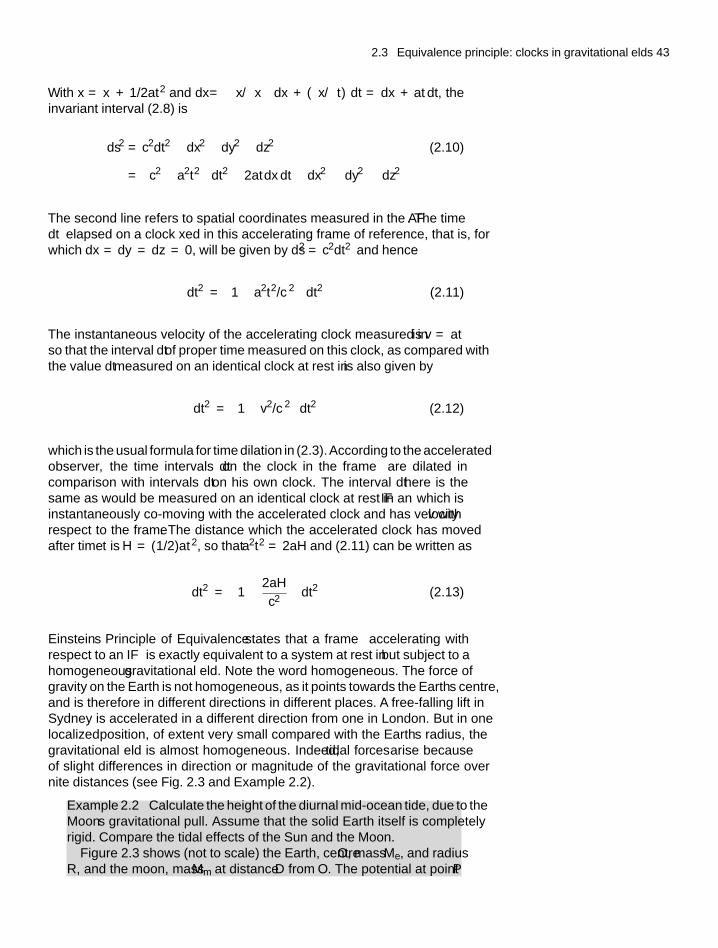
2.3 Equivalence principle: clocks in gravitational fields 43
With x = x′ + 1/2at2 and dx = (∂x/∂x′) dx′ + (∂x/∂t) dt = dx′ + at dt, theinvariant interval (2.8) is
ds2 = c2dt2 − dx2 − dy2 − dz2 (2.10)
=(
c2 − a2t2)
dt2 − 2at dx′dt − dx′2 − dy′2 − dz′2
The second line refers to spatial coordinates measured in the AF �′. The timedt′ elapsed on a clock fixed in this accelerating frame of reference, that is, forwhich dx′ = dy′ = dz′ = 0, will be given by ds2 = c2dt′2 and hence
dt′2 =(
1 − a2t2/c2)
dt2 (2.11)
The instantaneous velocity of the accelerating clock measured in � is v = atso that the interval dt′ of proper time measured on this clock, as compared withthe value dt measured on an identical clock at rest in � is also given by
dt′2 =(
1 − v2/c2)
dt2 (2.12)
which is the usual formula for time dilation in (2.3). According to the acceleratedobserver, the time intervals dt on the clock in the frame � are dilated incomparison with intervals dt′ on his own clock. The interval dt′ here is thesame as would be measured on an identical clock at rest in an IF �′′ which isinstantaneously co-moving with the accelerated clock and has velocity v withrespect to the frame �. The distance which the accelerated clock has movedafter time t is H = (1/2)at2, so that a2t2 = 2aH and (2.11) can be written as
dt′2 =(
1 − 2aH
c2
)dt2 (2.13)
Einstein’s Principle of Equivalence states that a frame �′ accelerating withrespect to an IF � is exactly equivalent to a system at rest in � but subject to ahomogeneous gravitational field. Note the word ‘homogeneous’. The force ofgravity on the Earth is not homogeneous, as it points towards the Earth’s centre,and is therefore in different directions in different places. A free-falling lift inSydney is accelerated in a different direction from one in London. But in onelocalized position, of extent very small compared with the Earth’s radius, thegravitational field is almost homogeneous. Indeed, tidal forces arise becauseof slight differences in direction or magnitude of the gravitational force overfinite distances (see Fig. 2.3 and Example 2.2).
Example 2.2 Calculate the height of the diurnal mid-ocean tide, due to theMoon’s gravitational pull. Assume that the solid Earth itself is completelyrigid. Compare the tidal effects of the Sun and the Moon.
Figure 2.3 shows (not to scale) the Earth, centre O, mass Me, and radiusR, and the moon, mass Mm at distance D from O. The potential at point P
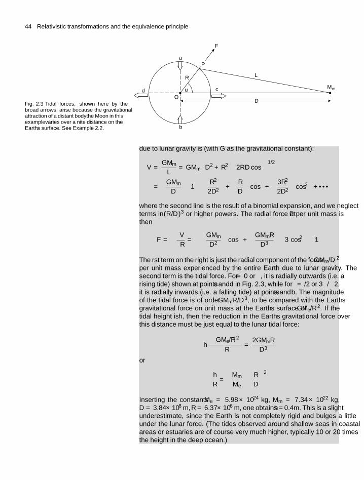
44 Relativistic transformations and the equivalence principle
Fig. 2.3 Tidal forces, shown here by thebroad arrows, arise because the gravitationalattraction of a distant body—the Moon in thisexample—varies over a finite distance on theEarth’s surface. See Example 2.2.
a
R
O
c
b
d u
D
L
Mm
P
F
due to lunar gravity is (with G as the gravitational constant):
V = GMm
L= GMm
(D2 + R2 − 2RD cos θ
)−1/2
=(
GMm
D
)[1 −(
R2
2D2
)+(
R
D
)cos θ +
(3R2
2D2
)cos2 θ + · · ·
]where the second line is the result of a binomial expansion, and we neglectterms in (R/D)3 or higher powers. The radial force at P per unit mass isthen
F = −∂V
∂R= −
(GMm
D2
)cos θ +
(GMmR
D3
) (3 cos2 θ − 1
)The first term on the right is just the radial component of the force GMm/D2
per unit mass experienced by the entire Earth due to lunar gravity. Thesecond term is the tidal force. For θ = 0 or π, it is radially outwards (i.e. arising tide) shown at points c and d in Fig. 2.3, while for θ = π/2 or 3π/2,it is radially inwards (i.e. a falling tide) at points a and b. The magnitudeof the tidal force is of order GMmR/D3, to be compared with the Earth’sgravitational force on unit mass at the Earth’s surface of GMe/R2. If thetidal height is h, then the reduction in the Earth’s gravitational force overthis distance must be just equal to the lunar tidal force:
h∂(GMe/R2
)∂R
= 2GMmR
D3
or
h
R=(
Mm
Me
)(R
D
)3
Inserting the constants Me = 5.98 × 1024 kg, Mm = 7.34 × 10²² kg,D = 3.84×10⁸ m, R = 6.37×10⁶ m, one obtains h = 0.4m. This is a slightunderestimate, since the Earth is not completely rigid and bulges a littleunder the lunar force. (The tides observed around shallow seas in coastalareas or estuaries are of course very much higher, typically 10 or 20 timesthe height in the deep ocean.)
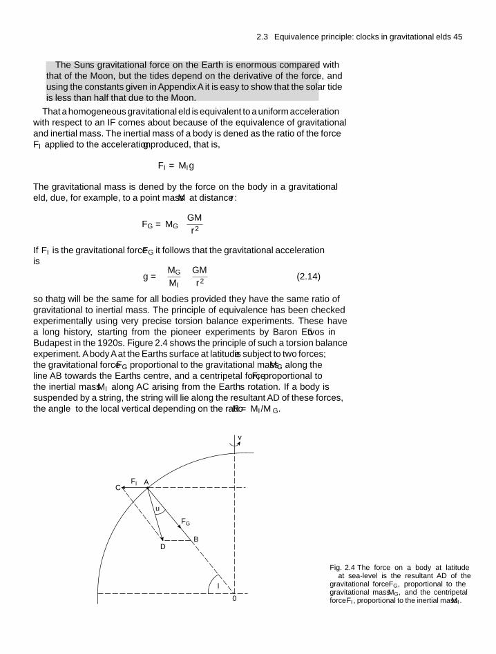
2.3 Equivalence principle: clocks in gravitational fields 45
The Sun’s gravitational force on the Earth is enormous compared withthat of the Moon, but the tides depend on the derivative of the force, andusing the constants given in Appendix A it is easy to show that the solar tideis less than half that due to the Moon.
That a homogeneous gravitational field is equivalent to a uniform accelerationwith respect to an IF comes about because of the equivalence of gravitationaland inertial mass. The inertial mass of a body is defined as the ratio of the forceFI applied to the acceleration g produced, that is,
FI = MIg
The gravitational mass is defined by the force on the body in a gravitationalfield, due, for example, to a point mass M at distance r:
FG = MG
(GM
r2
)If FI is the gravitational force FG it follows that the ‘gravitational acceleration’is
g =(
MG
MI
)GM
r2(2.14)
so that g will be the same for all bodies provided they have the same ratio ofgravitational to inertial mass. The principle of equivalence has been checkedexperimentally using very precise torsion balance experiments. These havea long history, starting from the pioneer experiments by Baron Eötvos inBudapest in the 1920s. Figure 2.4 shows the principle of such a torsion balanceexperiment. A body A at the Earth’s surface at latitude λ is subject to two forces;the gravitational force FG proportional to the gravitational mass MG along theline AB towards the Earth’s centre, and a centripetal force FI proportional tothe inertial mass MI along AC arising from the Earth’s rotation. If a body issuspended by a string, the string will lie along the resultant AD of these forces,the angle θ to the local vertical depending on the ratio R = MI/MG.
CFI
FG
BD
0
A
u
v
l
Fig. 2.4 The force on a body at latitudeλ at sea-level is the resultant AD of thegravitational force FG, proportional to thegravitational mass MG, and the centripetalforce FI, proportional to the inertial mass MI.
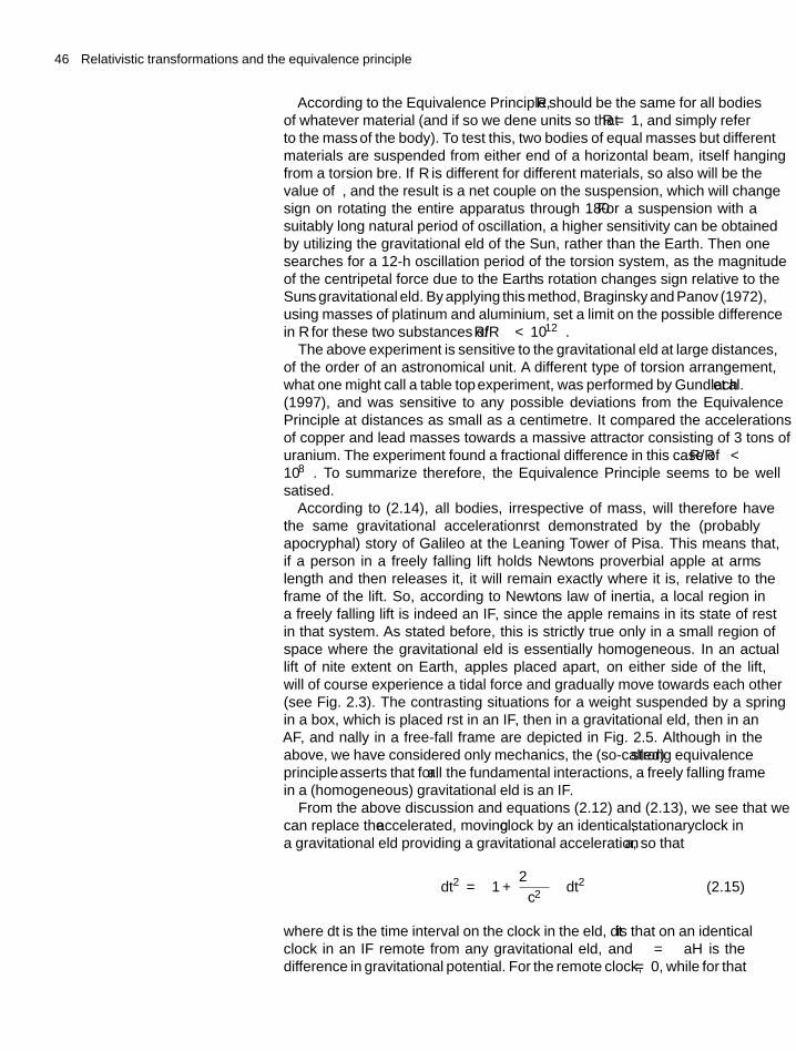
46 Relativistic transformations and the equivalence principle
According to the Equivalence Principle, R should be the same for all bodiesof whatever material (and if so we define units so that R = 1, and simply referto ‘the mass’ of the body). To test this, two bodies of equal masses but differentmaterials are suspended from either end of a horizontal beam, itself hangingfrom a torsion fibre. If R is different for different materials, so also will be thevalue of θ, and the result is a net couple on the suspension, which will changesign on rotating the entire apparatus through 180◦. For a suspension with asuitably long natural period of oscillation, a higher sensitivity can be obtainedby utilizing the gravitational field of the Sun, rather than the Earth. Then onesearches for a 12-h oscillation period of the torsion system, as the magnitudeof the centripetal force due to the Earth’s rotation changes sign relative to theSun’s gravitational field. By applying this method, Braginsky and Panov (1972),using masses of platinum and aluminium, set a limit on the possible differencein R for these two substances of �R/R < 10−12.
The above experiment is sensitive to the gravitational field at large distances,of the order of an astronomical unit. A different type of torsion arrangement,what one might call a ‘table top’ experiment, was performed by Gundlach et al.(1997), and was sensitive to any possible deviations from the EquivalencePrinciple at distances as small as a centimetre. It compared the accelerationsof copper and lead masses towards a massive attractor consisting of 3 tons ofuranium. The experiment found a fractional difference in this case of �R/R <
10−8. To summarize therefore, the Equivalence Principle seems to be wellsatisfied.
According to (2.14), all bodies, irrespective of mass, will therefore havethe same gravitational acceleration—first demonstrated by the (probablyapocryphal) story of Galileo at the Leaning Tower of Pisa. This means that,if a person in a freely falling lift holds Newton’s proverbial apple at arm’slength and then releases it, it will remain exactly where it is, relative to theframe of the lift. So, according to Newton’s law of inertia, a local region ina freely falling lift is indeed an IF, since the apple remains in its state of restin that system. As stated before, this is strictly true only in a small region ofspace where the gravitational field is essentially homogeneous. In an actuallift of finite extent on Earth, apples placed apart, on either side of the lift,will of course experience a tidal force and gradually move towards each other(see Fig. 2.3). The contrasting situations for a weight suspended by a springin a box, which is placed first in an IF, then in a gravitational field, then in anAF, and finally in a free-fall frame are depicted in Fig. 2.5. Although in theabove, we have considered only mechanics, the (so-called) strong equivalenceprinciple asserts that for all the fundamental interactions, a freely falling framein a (homogeneous) gravitational field is an IF.
From the above discussion and equations (2.12) and (2.13), we see that wecan replace the accelerated, moving clock by an identical, stationary clock ina gravitational field providing a gravitational acceleration a, so that
dt′2 =(
1 + 2��
c2
)dt2 (2.15)
where dt′ is the time interval on the clock in the field, dt is that on an identicalclock in an IF remote from any gravitational field, and �� = −aH is thedifference in gravitational potential. For the remote clock, � = 0, while for that

2.4 General relativity 47
g
(a) (b)
(c)
a = g
(d)
Fig. 2.5 A mass suspended from a springattached to the roof of a closed box, in fourcontrasting cases. In (a) the box is in aninertial frame, and the spring is not extended.In (b) the box is in a gravitational field,equivalent to an acceleration g, with thespring extended. In (c) the box is acceleratedwith an acceleration a = g with respectto an inertial frame, again with the springextended. Finally in (d) the box is in freefall in a homogeneous gravitational field, withno extension of the spring. Because of theequivalence principle, an observer inside thebox could not distinguish (b) from (c) or (d)from (a).
in the field, � < 0. Thus a clock at low (negative) gravitational potential, suchas one at sea-level, should run slower than an identical clock at a higher (lessnegative) potential on a mountain top. This predicted gravitational shift wasverified experimentally by Pound and Snider (1964). In their experiment, thevery small (10−15) increase in frequency f of 57Fe γ-rays falling down a vertical22-m tube was measured by means of an 57Fe absorber at the bottom, utilizingthe Mossbauer effect. The photons from the emitter at the higher potential are‘blue-shifted’ compared with the absorption frequency at the lower potential,and this was compensated using the Doppler effect, by slowly moving theabsorber downwards at the appropriate velocity v/c = � f / f ∼ 10−15. Sincethat time, atomic clocks have been carried on aircraft to directly verify theabove formula by comparing with similar clocks at ground level.
Relative to our remote clock at � = 0, a clock in the field of a point massM at distance r is at a potential � = −GM /r and
dt′2 =[
1 − 2GM(rc2) ] dt2 (2.16)
The analysis here has assumed small values of acceleration, that is, �� c2.It happens, however, that (2.15) and (2.16) are correct even for strong fields, andgive the same results as the full analysis using the general theory of relativity.
2.4 General relativity
Afull treatment of general relativity is lengthy and outside the scope of this text,and for such a treatment the reader is referred, for example, to the accompanyingbook in the Oxford Master Series Relativity, Gravitation and Cosmology byTa-Pei Cheng. Here, we just show the form of the Einstein field equations anddiscuss two important solutions, which we shall be using in later chapters.
In the special theory, equations of physics valid in all IFs could be expressedin terms of scalar and vector quantities (i.e. tensors of zero rank and first rank,respectively). In the general theory, however, the quantities occurring in the(so-called) covariant physical equations, valid in all reference frames, must
48 Relativistic transformations and the equivalence principle
be expressed as second-rank tensors. If we write the coordinates in (2.1) in adifferent notation, as ct = x0, x = x1, y = x2, z = x3 then (2.8) can be set inthe form of the space–time metric
ds2 =∑
gμv dxμ dxv =∑
dxμdxμ (2.17)
where the summation is over μ, ν = 0, 1, 2, 3, and gμν is a 4 × 4 matrix calledthe metric tensor.
Here, the coordinates have been labelled with upper (contravariant) indices,and the metric tensor with lower (covariant) indices, according to how theytransform under a change of coordinate system. Invariant scalars are alwaysa product of covariant and contravariant quantities. For coordinate frames ingeneral, including those accelerating with respect to IFs, the elements of gμν
will be a function of the space–time coordinates xμ. However, for IFs only, ithas a simple form with constant diagonal elements and all off-diagonal elementsequal to zero:
g00 = +1, g11 = g22 = g33 = −1; gμv = 0 for μ �= v. (2.18)
or set in matrix form
gμv =
∣∣∣∣∣∣∣∣1 0 0 00 −1 0 00 0 −1 00 0 0 −1
∣∣∣∣∣∣∣∣in conformity with (2.8).
In general relativity, the metric tensor, as the name implies, describes thegeometrical properties of space/time, and in particular how it differs fromthe ‘flat’ so-called Minkowski metric of special relativity. Einstein had indeedinterpreted gravitational effects as due to the geometry of space, which changesin the presence of masses that introduce curvature or ‘warping’. The mostimportant quantity in describing deviations from flat space is the Riemanncurvature tensor, which is a function of the derivatives of gμν. From this one canderive quantities called the Ricci tensor Rμν and the Ricci scalar R = gμνRμν.These enter into the expression for the Einstein tensor, Gμv = Rμv−(R/2) gμv.This tensor is symmetric (Gμν = Gνμ) and has zero divergence, and Einstein’sleap of genius was to propose that it should be proportional to the energymomentum tensor Tμν, which, due to conservation of energy and momentum, isalso symmetric and divergenceless. He deduced the constant of proportionalityfrom Newton’s law of gravitation in the non-relativistic, weak field limit. Thenthe Einstein field equations become, with G as Newton’s gravitational constant:
Gμv = −8πGTμv
c4(2.19)
There are in all 4×4 = 16 equations, but because of the symmetry of Gμν, thisreduces to 10, of which only 6 are independent. In the static limit, the relevantμ = ν = 0 components are G00 = −2∇2�/c2 and T00 = ρc2, where � is thegravitational potential and ρ is the matter density. In this limit the above set of
2.5 Schwarzschild line element, radius, and black holes 49
equations then become Poisson’s equation of Newtonian gravity
∇2� = 4πGρ (2.20)
For a spherically symmetric potential, ∇2� = (1/r2) [
∂(r2∂�/∂r
)/∂r],
which upon integration gives
� (r) = 2πGρr2
3
and for the field due to a point mass M at the origin r = 0, Newton’s inversesquare law becomes
F (r) = ∂�
∂r= GM
r2
The foregoing paragraphs have been inserted simply to show the form of theEinstein field equations. Two important solutions are quoted in the followingparagraphs.
2.5 The Schwarzschild line element,Schwarzschild radius, and black holes
A very important solution of the Einstein field equations of general relativity isthat obtained by Schwarzschild in 1916, for the metric in the neighbourhood ofa spherically symmetric distribution of total mass M , far removed from othergravitating masses. In this case the elements of the metric tensor are no longerconstant as in (2.18), but functions of the coordinates. The Schwarzschild lineelement has the form
ds2 =[
1 − 2GM(rc2) ] c2dt2 −
[1 − 2GM(
rc2) ]−1
dr2 − r2(
dθ2 + sin2 θ dϕ2)
(2.21)where the spherical polar coordinates t, r, θ, and ϕ are those measured by anobserver in an IF, that is, a frame in free fall with respect to the mass M . If weset dr = dθ = dϕ = 0, the proper time interval dτ is given by dτ2 = ds2/c2,as measured on a clock at rest in the gravitational field of the mass M . Fromthe first term on the right-hand side of the above equation we see that this isreduced in comparison with the value dt on an identical clock in the (free-fall)IF, according to
dτ =√√√√[1 − 2GM(
rc2) ] · dt (2.22)
as indicated already in (2.16). A clock in a gravitational field runs slow! Whenthe clock is placed at the radial coordinate r = 2GM /c2, dτ = 0, so that thetime on the local clock appears to be frozen. The quantity
rs = 2GM
c2(2.23)
is called the Schwarzschild radius of the mass M . What does this mean?Consider a particle with velocity v approaching the mass M in a radial direction.
50 Relativistic transformations and the equivalence principle
The inward acceleration it experiences is
dv
dt= −v
dv
dr= GM
r2
On integrating, assuming v = 0 at r = ∞, we obtain for the velocity at radius r
v2 = 2GM
r
Reversing the path of the particle, we see that v is the escape velocity at r.Therefore the meaning of the Schwarzschild radius in (2.23) is that the escapevelocity at this radius is v = c, and hence no particle, not even a photon,can escape from inside it. Thus it appears as a black hole. We also note that thefrequency of light at the Schwarzschild radius goes to zero (i.e. the gravitationalredshift is infinite) as demonstrated by the Doppler shift formula (2.36) below.A discussion of the Schwarzschild radius and experimental evidence for blackholes is given in Chapters 9 and 10.
The formula (2.21) can be used to calculate the deflection of light-rays bythe gravitational field of the mass M , and it provided an early verification ofEinstein’s general theory of relativity. With the help of special relativity andthe equivalence principle, we may note here that the form of the Schwarzschildsolution can in fact be understood from purely heuristic arguments. In fact, theequivalence principle was already used by Einstein in arriving at his generaltheory. The treatment here follows that presented by Adler, Balzin, and Schiffer(1965) by determining the factors which connect the expression for the intervalin an IF to that in a frame at rest in the gravitational field of the isolated pointmass M (at r = 0), which we refer to as the AF. In the IF, the interval in sphericalcoordinates will be given by the special relativity formula (2.9):
ds2 = c2dt2 − dr2 − r2(
dθ2 + sin2 θ dϕ2)
(2.24)
where for a photon, ds2 = 0. According to the equivalence principle, the lengthof a standard rod at rest in the AF, as measured by the free-falling IF observerin the (radial) direction of the acceleration, appears contracted relative to anidentical rod at rest in the IF. The (length)2 is reduced by a factor
(1 − v2/c2
) =(1 − 2GM /rc2
), where v is the instantaneous velocity at r of the free-fall IF
with respect to M . On the other hand, the time interval on a clock at rest in theAF appears dilated when measured by the IF observer, as compared with anidentical clock at rest in the IF, because a clock in a gravitational field runs slow.
The (time interval)2 is increased by a factor(1 − 2GM /rc2
)−1as in (2.16). The
spherical symmetry of the problem means that these factors depend only on theradius vector r. From the values of t, r, θ, and ϕ and their increments, nowmeasured in the presence of the gravitational field by the IF observer, we cantherefore obtain the expression for the interval by dividing by the above factors.So (2.24) becomes
ds2 = c2(
1 − 2GM
rc2
)dt2 −
(1 − 2GM
rc2
)−1
dr2 − r2(
dθ2 + sin2 θ dϕ2)
in conformity with the Schwarzschild line element (2.21). Note that we have notderived this transformation from first principles, but merely shown that (2.21)
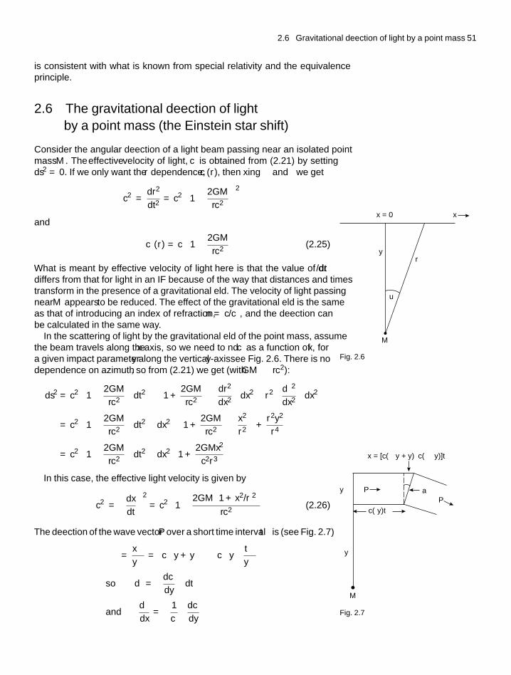
2.6 Gravitational deflection of light by a point mass 51
is consistent with what is known from special relativity and the equivalenceprinciple.
2.6 The gravitational deflection of lightby a point mass (the Einstein star shift)
Consider the angular deflection of a light beam passing near an isolated pointmass M . The effective velocity of light, c′ is obtained from (2.21) by settingds2 = 0. If we only want the r dependence, c′(r), then fixing θ and ϕ we get
c′2 = dr2
dt2= c2
(1 − 2GM
rc2
)2
and
c′ (r) = c
(1 − 2GM
rc2
)(2.25)
What is meant by ‘effective velocity of light’ here is that the value of dr/dtdiffers from that for light in an IF because of the way that distances and timestransform in the presence of a gravitational field. The velocity of light passingnear M appears to be reduced. The effect of the gravitational field is the sameas that of introducing an index of refraction, n = c/c′, and the deflection canbe calculated in the same way.
In the scattering of light by the gravitational field of the point mass, assumethe beam travels along the x-axis, so we need to find c′ as a function of x, fora given impact parameter y along the vertical y-axis—see Fig. 2.6. There is nodependence on azimuth ϕ, so from (2.21) we get (with GM rc2):
y
M
x = 0 x
r
u
Fig. 2.6
ds2 = c2(
1 − 2GM
rc2
)dt2 −
(1 + 2GM
rc2
)(dr2
dx2
)dx2 − r2
(dθ2
dx2
)dx2
= c2(
1 − 2GM
rc2
)dt2 − dx2
[(1 + 2GM
rc2
)(x2
r2
)+ r2y2
r4
]= c2
(1 − 2GM
rc2
)dt2 − dx2
(1 + 2GMx2
c2r3
)
�y
y
M
�aP
c�(y)�t
�x = [c�(y + �y) – c�(y)]�t
P
Fig. 2.7
In this case, the effective light velocity is given by
c′2 =(
dx
dt
)2
= c2
[1 − 2GM
(1 + x2/r2
)rc2
](2.26)
The deflection of the wave vector P over a short time interval �t is (see Fig. 2.7)
�α = �x
�y= [c′ (y + �y
)− c′ (y)] �t
�y
so dα =(
dc′
dy
)dt
anddα
dx=(
1
c′
)dc′
dy
52 Relativistic transformations and the equivalence principle
Since the difference between c′ and c is very small, we can set c′ = c in thedenominator. From (2.26) we therefore find(
1
c′
)dc′
dy=(
GM
r2c2
)[y
r+ 3x2y
r3
]In the scattering process, the value of y is essentially constant and equal to
the impact parameter, y = b, say. Then
dα
dx=(
1
c
)dc′
dy=(
GM
c2r2
)[b
r+ 3x2b
r3
](2.27)
With r = b sec θ, x = b tan θ, dx = b sec2 θdθ one obtains for the deflection oflight associated with the passage of the beam through the angular interval dθ:
dα =(
GM
c2b2
)[cos3 θ + 3 sin2 θ cos3 θ
]b sec2 θ dθ
and α =(
GM
c2b
)∫ (1 + 3 sin2 θ
)d (sin θ)
Inserting the limits of the integral, θ = π/2 and θ = −π/2 we obtain for thedeflection
α = 4GM
c2b(2.28)
As is well known, the deflection of light from stars close to the Sun was firstmeasured, and the predicted value of 1.75 arcsec (8.48 μrad) from (2.28), wasverified by Eddington and others in the 1919 eclipse expedition to Principe andSobral. It was a first confirmation of Einstein’s general theory of relativity.
2.7 Shapiro time delay
The gravitational field due to a point mass M introduces, as well as an angulardeflection, a time delay, on light (or any electromagnetic pulse) passing nearby.It is called the Shapiro delay, named after the physicist who was first to realizeits existence. It arises because of the ‘curvature’ or ‘warping’ of space, whichsends photons on a slightly longer path. This time delay was first observed bybouncing radar pulses from Mercury and Venus and observing the delay of thereturn pulse as the line of sight to these planets moved near to the Sun. Tocalculate the effect, we neglect the tiny angular deflection in (2.28), so thatfrom (2.26) the increment of transit time over the path element dx becomes (forGM rc2)
dt = dx
c′ =(
dx
c
)[1 +(
GM
rc2
)(1 + x2
r2
)]and the total transit time, from x = 0 to x = X is (changing variables tox = b tan θ)
t =(
X
c
)+(
GM
c3
)∫dθ
(1 + sin2 θ
)cos θ
2.8 Orbital precession 53
where θ varies from 0 at x = 0 to θm = tan−1 (X /b) for x = X . Thus theintegrated time delay over the interval x = 0 to x = X becomes
�t =(
GM
c3
)[2 ln
{tan
(θm
2+ π
4
)}− sin θm
]
≈(
GM
c3
)[2 ln
(2X
b
)− 1
](2.29)
where the approximate form, obtained by expanding the circular functions, isgood to better than 0.2% for X > 10b. In a practical case, we can take for M thesolar mass and for the impact parameter b the solar radius. Setting X equal tothe Earth–Sun distance, then for return pulses grazing the Sun from a planet atdistance, say 2X from Earth, the total time delay for the out-and-return journeywill be 4�t ∼ 230μs.
2.8 Orbital precession
Another early success of general relativity was the correct prediction of thetiny precession of the axes of the elliptical orbits of the planets. The historicalcase was that of the planet Mercury. The actual precession observed was of 532arcsec per century, of which all but 43 arcsec could be accounted for by tidalforces due to other planets. Before Einstein’s theory, the discrepancy had beenattributed to the existence of an extra planet (Vulcan) which, however, wasnever found. According to the general theory, for the case of ‘weak fields’ thereis, in addition to the usual 1/r2 Newtonian term, a small extra term varying as1/r4 in the gravitational force. This has the result that the orbit is no longer atotally closed ellipse with fixed axes, but can be interpreted as a closed ellipticorbit in which the axis advances slowly with time. The resulting advance inthe angle of rotation ϕ can be calculated, starting from the Schwarzschild lineelement (2.21), and applying the Euler–Lagrange equation (see Chapter 3) todeduce the equation of the orbit. For a circular orbit of radius r the fractionaladvance is found to be (for r � rs):
�ϕ
ϕ= 3rs
2r= 3u2
c2(2.30)
where rs = 2GM /c2 is the Schwarzschild radius of the Sun, mass M , and u isthe orbital velocity (with u2 = GM /r). Again we may note that this formula canbe understood on the basis of the equivalence principle and special relativity, asfollows. The angular momentum of the planet L = m (r × u) = mr2dϕ/dt is aconstant1 (Kepler’s second law). Using the same arguments following equation 1L is normal to the orbit plane, so is
unaffected by the above transformation.(2.24), and transforming from the accelerated frame to an IF, the quantityr2 will be contracted by a factor (1 − rs/r), while the time t will be dilatedby a factor 1/(1 − (rs/2r)). So ϕ (or
∫dt/r2) must be increased by a factor
(1 + 3rs/2r).
54 Relativistic transformations and the equivalence principle
For an elliptic orbit of eccentricity e and semimajor axis a, the radius vectorr is given by
1
r= (1 + e cos ϕ)[
a(1 − e2
)]Integrating over ϕ to find an averaged value,
∫(1/r) dϕ/2π, it follows that
for an elliptic orbit, 1/r in (2.30) must be replaced by 1/[a(1 − e2
)]. From
the values of the constants for the Sun and Mercury (see Problem 2.1), theabove formula yields a value for the precession of 42.9 arcsec per century. Thefact that the calculated and observed precessions agreed within 1% was a dualtriumph, for the theory of relativity and for the precision measurements of theastronomers. Larger orbital precessions are expected for stronger fields, themost marked example so far being the 17◦ precession per year for the twinpulsars PSR J0737-3039 (see Chapter 10).
It should be noted that all the tests in Sections 2.6–2.8 are for weakgravitational fields, providing small, linear, perturbative corrections toNewtonian mechanics. General relativity has emerged from these and othertests with flying colours. However, more crucial tests would be for very strongfields, where the effects of non-linearities in the Einstein field equations shouldbe manifest.
2.9 The Robertson–Walker line element
The Friedmann–Lemaitre–Robertson–Walker model of the universe (FLRWfor short), which forms part of the ‘Standard Model’of cosmology, is discussedin Chapter 5. Here, we just note that this is the simplest model, based onthe concept of an originally isotropic and homogeneous expanding universewith a uniform space–time curvature. The line element (2.9) appropriate to IFsin special relativity is modified in general relativity for the FLRW model asfollows:
ds2 = c2dt2 − R (t)2
[dr2(
1 − kr2) + r2 dθ2 + r2 sin2 θ dφ2
](2.31)
where R(t) is a universal expansion parameter, which multiplies the radial spacecoordinate r defined in a reference frame co-moving (i.e. enlarging ) with theexpansion, so that the physical coordinate distance D from one point to another(anywhere in the universe since it is assumed to be isotropic and homogeneous)is written as the product
D (t) = r · R (t) (2.32)
All the time dependence of distances between points is contained in theexpansion factor R(t). The time at which one measures R can be universal in thismodel, since observers can in principle be scattered all over the universe, andthey can agree to synchronize their identical clocks when the universal densityof expanding matter reaches a specified value. The parameter k describes thecurvature of space. k = +1 corresponds to positive curvature, k = −1 to negativecurvature and k = 0 to the flat Euclidean space of special relativity.
Equation (2.31) follows from general relativity for the particular case of anisotropic and homogeneous universe undergoing an isotropic expansion with
2.10 Modifications to Newtonian gravity? 55
a uniform curvature k/R2, and we have simply stated the result. However, theform of the curvature term affecting the radial coordinate can be understoodfrom a two-dimensional analogy. Figure 2.8 shows a section through a sphereof radius ρ, centre O, and two points on the surface of the sphere A and B. Theshortest distance between A and B along the surface is the arc AB of a greatcircle, of length 2l. Denote the angle subtended at the centre by 2α = 2l/ρ andthe chord AB through the sphere by 2D, where D = ρsinα. Then
A BD
r
O
a
l
Fig. 2.8
D = ρ sin
(l
ρ
)
dD = cos
(l
ρ
)dl
and
dl = dD
cos (l/ρ)= dD√
1 − D2/ρ2
If we define the curvature 1/ρ2 = k/R2, where k = +1 in this case, then withD = Rr as above, we obtain
dl = R dr√1 − kr2
(2.33)
This is the form in (2.31) expressing the element of arc length dl along thesurface of the sphere in terms of the curvature parameter k and the element ofchord length dD = Rdr. This two-dimensional analogy in fact carries straightover to three (or any larger number) of spatial dimensions, because of the spatialisotropy assumed in the model. However, this analogy applies for k = +1 onlyand there is no two-dimensional analogue for k = −1.
When the FLRW metric (2.31) is inserted into the field equations (2.19),there results the very important Friedmann equation(s) described in Chapter 5.Equation (2.31) is one of the key equations in cosmology and will be usedfrequently in the following chapters.
2.10 Modifications to Newtonian gravity?
The inverse square law of gravitational force (for weak gravitational fields andin the non-relativistic approximation) is known to hold with great accuracy forthe solar system, that is, for distances within a few orders of magnitude of theastronomical unit. However, at much larger distances, that is, on the scale ofour universe (giga parsec or 1026 m) it has been proposed that modificationsmay occur, and that these are responsible for the fact that 95% of the energydensity of the universe appears to be due to the existence of completely newforms of dark matter/dark energy, as described in Chapter 7. At the presenttime, despite extensive searches, there is no direct experimental evidence fordark matter, for example, in the form of new elementary particles which canbe detected and measured in the laboratory. So, could it be that it is all anartefact of deviations from the inverse square law at very large distances? Asdescribed in Section 7.4, there is absolutely no indication that this is the case,and that indeed examples are known of distant colliding galaxies in which the
56 Relativistic transformations and the equivalence principle
visible, luminous matter, subject to electromagnetic forces in collision, is wellseparated from the dark matter, subject to and identified from its gravitational(lensing) effects. No modifications to the inverse square law could possiblyaccount for these phenomena.
One can also question the inverse square law at very small distances. Theenergy density of dark energy (about 5 GeV m−3) when expressed in naturalunits (h = c = 1), can be used to define a fundamental length, of about 85μm (see Section 7.4). Could it be that the dark energy is somehow associatedwith deviations from the inverse square law at such distances, connected withthe idea that the weakness of gravity compared with the other interactions isdue to extra dimensions which at normal energies, well below the Planck scale,are curled up and ineffective? The torsion balance experiments of Kapner et al.(2007), however, have verified Newton’s law with great accuracy down todistances of around 50 μm.
To summarize, over the years physicists, for one reason or another, havequestioned the validity of Newton’s inverse square law (always of course in thestatic, non-relativistic approximation to the Einstein equations) over distancescales covering at least 30 orders of magnitude. All the evidence so far, however,corroborates Newton’s law.
2.11 Relativistic kinematics: four-momentum;the Doppler effect
The transformations of energy and momentum of a particle between IFs inspecial relativity are easily found from the coordinate transformations (2.1) byreplacing x, y, z by the Cartesian components px, py, pz of the three-momentump of the particle, and the time component t by the total energy E (using unitsc = 1 for brevity). Then the transformations between an IF � and anotherframe �′ moving at velocity βc in the x-direction with respect to � are
p′x = γ
(px − βE
)p′
y = py
p′z = pz (2.34)
E′ = γ(E − βpx
)where γ = (1 − β2)−1/2, and the quantity
E′2 − p′2 = E2 − p2 = m2 (2.35)
where m, the rest-mass of the particle, is invariant under the transformation.The above transformations give the formula for the Doppler effect in
relativistic optics. Consider a light beam of frequency ν and quantum energyE = hν emitted in the frame � at an angle θ with respect to the x-axis. From(2.34) the energy E′ = hν′ in the frame �′ will be (since p = E for photons in
2.12 Fixed-target and colliding-beam accelerators 57
our units of c = 1)
E′ = γE (1 − β cos θ)
and for θ = 0,
v′ = γv(1 − β) = v
√(1 − β)
(1 + β)(2.36)
Thus a source of light travelling at velocity βc away from an observer has itsfrequency ‘red-shifted’ by a factor v′/v. For θ = π/2, one obtains a transverseDoppler effect, with
v′ = γv = v
(1 + β2
2+ · · ·
),
so it is second-order in β for small values of β, while for θ = 0 it is first order.We already saw in (2.8) that the expression for the square of the interval
ds was an invariant under a transformation to another IF. The quantity ds iscalled a four-vector, since it has four space and time components, and theinvariance under Lorentz transformations is analogous to the invariance in threespace dimensions, of the length squared of a three-component vector undertranslations or rotations of the coordinate axes.
In kinematics we express the quantities in (2.34) as components of four-vectors called four-momenta pμ (μ = 0, 1, 2, 3), where for a single particlep0 = E, p1 = px, p2 = py, p3 = pz . The four-momentum squared is a Lorentzscalar with the value (in units c = 1)
p2 = E2 − |p|2 = m2 (2.37)
In scattering experiments in high-energy physics, the result of the scatteringof a particle by the interaction can be expressed in terms of the invariant four-momentum transfer qμ = pμ − p′
μ, so that q2 = (E − E′)2− (p − p′)2, wherethe unprimed and primed quantities refer to the values for a particle before andafter the interaction. It is left as an exercise to show that q2 is always negativein a scattering process.
In kinematic problems, it is advantageous to evaluate quantities in the centre-of-momentum system (CMS) that is in a coordinate frame where the totalthree-momentum p of the colliding particles is zero. Then the invariant four-momentum squared (which can be evaluated in any IF) is just equal to the squareof the total CMS energy, conventionally denoted by the symbol s = E2
CMS (butnot to be confused with the space–time interval, also called s).
2.12 Fixed-target and colliding-beamaccelerators
As an example of the use of four-vectors and the centre-of-momentum frame ofreference, we consider fixed-target and colliding-beam accelerators. Supposea beam of particles of mass ma, energy Ea, and three-momentum pacollides
58 Relativistic transformations and the equivalence principle
with a target particle of mass mb, energy Eb, and momentum pb. Then the totalfour-momentum squared is given by
s = (Ea + Eb)2 − (pa + pb
)2 = m2a + m2
b + 2(EaEb − pa · pb
)(2.38)
The energy available for new particle creation is ε = (√
s−mb - ma). If Ea � ma
and Eb � mb, thenε2 ≈ 2
(EaEb − pa · pb
)(2.39)
(a) Fixed Target
If the beam of a particles collides with a stationary target b, so that Eb = mband pb = 0, then
ε ≈ (2mbEa)1/2 (2.40)
and the available energy rises with the square root of the incident energy.Examples of accelerators that have used fixed targets are the CERN PS (ProtonSynchrotron) accelerating protons to 28 GeV, and the CERN SPS (Super ProtonSynchrotron) for protons up to 400 GeV.
(b) Colliding beams
If the beams of a and b particles collide head-on, then pa · pb = −|pa||pb| andassuming both beams are extreme relativistic, we obtain
ε ≈ [2 (EaEb + |pa| |pb|)]1/2 ≈ √4EaEb
In many colliders, the two beams are of particles of equal masses and equalenergies, that is, Ea = Eb = E, when
ε ≈ 2E (2.41)
so that the available energy rises in proportion to the beam energy. An exampleis the LEP II e+e− collider at CERN, which accelerated electrons and positronsin opposite directions in the same vacuum tube. The beam energies were E =100 GeV, so that the 200 GeV available CMS energy was sufficient to investigatethe reactions e+e− → W +W − and Z0Z0, where the threshold energies are2MW ∼ 160 GeV and 2MZ ∼ 180 GeV. The HERA machine is an exampleof an asymmetric ep collider, accelerating electrons or positrons to 28 GeVenergy in one vacuum ring, and protons to 820 GeV in the other directionin a second ring above the first, the two beams being brought into collisionin two intersection regions. In this case, the square of the CMS energy iss = 93, 000 GeV2, and the useful maximum value of four-momentum transfersquared between the particles is |q2(max)| ∼ 20,000 GeV2, about 100 timesthe maximum useful value attainable using secondary muon or neutrino beamsfrom fixed-target machines.
Colliding-beam machines have the obvious advantage of providing muchhigher CMS energies for a given beam energy, and have been essential inidentifying the more massive fundamental particles—the W ± and Z0 mediatorsof the electroweak interactions and the bottom and top quarks during the 1980sand 1990s. They are, however, limited to beams of stable or nearly stable
Problems 59
particles, namely electrons, positrons, protons, antiprotons, heavy ions, andpossibly in the future, muons (in μ+μ− colliders).
Fixed-target machines achieve lower CMS energies but have the advantagethat they can produce a range of intense high-energy beams of secondaryparticles, for example, π, K±, K0, μ, νμ. These were important historically, inlaying the quantitative experimental foundations of particle physics, includingthe establishment of the quark substructure of matter and of CP violation inweak interactions in the 1960s, and of the electroweak theory and quantumchromodynamics of the strong interquark interactions in the 1970s. They stillhave very important applications today both as injectors for colliders and assources of neutrino beams for the study of neutrino oscillations.
Problems
At the end of the book, answers are given to all the problems. Fullsolutions are given to the more challenging problems, which aredenoted by an asterisk.
(2.1) Calculate the precession of the orbit of Mercury from(2.30), given the following data:
Mercury mass = 3.24 × 10²³ kg.Semimajor axis = 0.387 A.U.
Eccentricity = 0.206Earth mass = 5.98 × 1024 kg.
Sun mass = 1.99 × 1030 kg.
(2.2) Calculate the maximum value of the square of themomentum transfer q2 in (GeV/c)2, in the head-oncollision at the HERA collider of a 28 GeV electronwith a quark carrying 20% of the energy of an 800GeV proton.
(2.3) The neutral pion undergoes the decay π0 → 2γ .Because the pion has spin zero, the angular distributionof the γ-rays in the pion rest frame is isotropic. Theγ-rays from decay of pions produced by cosmic raycollisions in the atmosphere are observed. Show thattheir energy spectrum has a peak intensity for Eγ =mπc2/2, and that if E1 and E2 are the two γ energieson either side of this maximum for which the γ-rayintensities are equal, then
√E1E2 = mπc2/2. (Note:
this method was used in 1950 to obtain one of theearliest measurements of the neutral pion mass).
(2.4) A photon of wavelength λ is emitted from the solarsurface. Calculate the shift �λ in wavelength of thephoton when it arrives at the Earth’s surface.
(Solar mass and radius 1.99 × 1030 kg, 6.96 ×10⁸ m
Earth mass and radius 5.98 × 1024 kg, 6.37 × 10⁶ m.)
*(2.5) Using the transformations of momentum and energy inSection (2.11), derive an expression for the laboratoryangle of emission of a γ-ray by an unstable particlein terms of the angle of emission in the rest-frame ofthe particle. Thus show that for a beam of very high-energy particles, half the γ-rays will be concentratedinside a forward cone of opening angle θ oforder 1/γ .
(2.6) Asatellite travels in a circular orbit about the Earth witha period of 12 h. Calculate the fractional difference(with sign) in time between a satellite clock and anidentical clock on the Earth. Refer to Question (2.4)for the Earth mass and radius. Neglect the effect ofthe Earth’s rotation. (This problem has a practicalapplication in correcting the times on the atomic clocksof the satellites used in the Global Positioning System.)
3Conservation rules,symmetries, and theStandard Model ofparticle physics
3.1 Transformations and the Euler–Lagrangeequation
One of the most important concepts in physics is that of the symmetry orinvariance of a system under a particular operation. For example, a snowflake isinvariant under a 60◦ rotation in the plane of the flake, and this tells us somethingabout the physics of the molecular bonding in water. In fact, conservation rulesand the associated symmetries have been called the backbone of high-energyparticle physics.
Not all conservation rules are absolute. While conservation of electric chargeor of energy and momentum are, as far as we know, sacrosanct in all situations,some quantities—for example, conservation of parity—that is, invariance underspatial reflection—hold for certain types of fundamental interaction but not forothers. Moreover, on the enormous distance and time scales of the universeat large, it turns out that some quantum numbers, such as baryon number,which seem to be exactly conserved under laboratory conditions, are violatedin cosmology. This violation presumably occurred at a very early, very hot stageof the universe, involving some new type of interaction at energies far abovewhat can be obtained by accelerators on Earth.
The invariant description of physical phenomena in relativity, that is, undertransformations of space and time coordinates, has been discussed in Chapter 2.In this chapter, we first of all discuss some of the important conservation rulesand symmetries, and later describe the broken symmetries, including thosewhich we believe have been at the core of the early development of the universe,described also in Chapter 4.
One familiar conservation law is that of linear momentum in classicalmechanics, which follows if the energy of the system is invariant undertranslations in space. For, if there is no change in energy under such atranslation, there can be no external forces on the system and the rate ofchange of momentum must be zero. This last example can be formalized by theEuler–Lagrange equation of classical mechanics. This is based on Hamilton’s‘principle of least action’. The Lagrangian function in this case is the differenceof kinetic and potential energies, L = T − V , for a set of particles. The actionS = ∫ Ldt and the above principle states that the path between fixed startingand ending coordinates q(t1) and q(t2) travelled by a particle between times t1
3.1 Transformations and the Euler–Lagrange equation 61
and t2 is such that the action is at an extremum (corresponding in fact to theshortest path in space or to the maximum path in proper time). For example,denoting the space coordinate by q and the velocity q = dq/dt as independentvariables, we can write for the perturbation in the action due to a variation δqfrom the ‘classical path’ traced by the particle as
δS =∫ [(
∂L
∂q
)δq +
(∂L
∂q
)δq
]dt = 0
Since δq = d(δq)/dt, we can integrate the second term in the integrand by
parts to obtain
∫ (∂L
∂q
)δq dt =
[δq
(∂L
∂q
)]−∫
δq
[d(∂L/∂q
)dt
]dt
For the limits of integration, which are at the fixed endpoints of the path, δq = 0,so the first term on the right-hand side vanishes. Hence,
∂S =∫ {(
∂L
∂q
)− d(∂L/∂q
)dt
}δq dt = 0
Since this must be true for arbitrary values of δq, the integrand must be zero,and the Euler–Lagrange equation follows:
∂L
∂q− d
dt
(∂L
∂q
)= 0 (3.1)
Thus if L is independent of q, ∂L/∂q = 0 and the momentum p = ∂L/∂q isconstant. Here a global symmetry—invariance of L under space translations—has led to a conservation law. In this case we have taken the independentvariables as the space coordinate q and the momentum p, but (3.1) can representany pair of generalized coordinates, one being a derivative of the other.
In relativistic quantum mechanics, the Lagrangian function L is a field energydensity rather than a sum over the energies of discrete particles, and it isfurthermore a function of both space and time. The global invariance of Lunder space–time translations leads to a conserved current of four momentum,which is an example of a more general theorem called Noether’s theorem,discussed in Section 3.8 below. The conservation of the fourth (time) componentof this current corresponds to conservation of energy, and of the three spacecomponents to conservation of momentum.
The invariance (or non-invariance) of a physical system may occur forcontinuous transformations, for example, a rotation in a phase angle or atranslation in space; or it can be a discrete transformation, such as theinversion of a spatial or time coordinate, or charge conjugation. For continuoustransformations, the associated conservation laws and quantum numbers areadditive (the total conserved energy of system is equal to the sum of the energiesof its parts), while for discrete transformations they are multiplicative (e.g. thesymmetry under spatial reflection, called the parity, is equal to the product ofthe parities of the parts of the system).
62 Conservation rules, symmetries, and Standard Model of particle physics
3.2 Rotations
As an example of a continuous transformation let us consider a spatial rotationthrough some angle, say φ, about the z-axis. The operator of the z componentof angular momentum in Cartesian coordinates is defined as
Jz = −ih
(x
∂
∂y− y
∂
∂x
)This operation can also be described by a rotation. Suppose a vector of lengthr lying in the xy plane makes an angle φ with the x-axis. Then in a rotationthrough δφ, the increments of the Cartesian components are
δy = r cos φ δφ = xδφ
δx = −r sin φ δφ = −yδφ
The effect of this rotation on a function ψ(x, y, z) will be
R (φ, δφ) ψ(x, y, z
) = ψ(x + δx, y + δy, z
) = ψ(x, y, z
)+ δx
(∂ψ
∂x
)+ δy
(∂ψ
∂x
)=ψ
[1 +(
x∂
∂y− y
∂
∂x
)]=y
[1 + δφ
∂
∂φ
]Hence the Jz operator
Jz = −ih
[x
∂
∂y− y
∂
∂x
]= −ih
∂
∂φ
Afinite rotation is achieved by making n infinitesimal steps, that is, �φ = nδφ
where n → ∞, so that
R = Limn→∞
(1 + iJz
δφ
h
)n
= exp
(iJz
�φ
h
)(3.2)
Here Jz is said to be the generator of the rotation �φ.
3.3 The parity operation
The inversion of spatial coordinates (x, y, z) → (−x, −y, −z) is a discretetransformation on the wave amplitude ψ brought about by the parity operatorP : Pψ(r) = ψ(−r). Since in repeating the operation one reverts to the originalsystem, P2 = 1 and the eigenvalues of P must be ±1. These eigenvalues arereferred to as the parity of the system ψ. For example, the function ψ = cos xhas P = +1 or positive parity since Pψ = P(cos x) = cos(−x) = +ψ, whileif ψ = sin x, Pψ = −ψ so that ψ has negative parity. On the other hand, in thecase of a function such as ψ = (sin x + cos x), Pψ = (cos x − sin x) �= ±ψ
so this function is not an eigenstate of parity. Parity is a useful concept whendealing with elementary particles since the interactions often have very well-defined properties under the parity operation. This may be contrasted withbiological systems, for example, a runner bean or the DNA molecule, whichare not eigenstates of parity.
3.4 Parity conservation and intrinsic parity 63
A spherically symmetric potential has the property that V (−r) = V (r), sothat states bound by such a potential—as is usually the case in atoms—can beparity eigenstates. For the hydrogen atom, the wavefunction in terms of theradial coordinate r and the polar and azimuthal angular coordinates θ and φ ofthe electron with respect to the proton is
χ (r, θ, φ) = η (r) Y ml (θ, φ)
where Y is the spherical harmonic function, with l the orbital angularmomentum quantum number and m its z-component. Under inversion, r →−r, θ → (π − θ), while φ → (π + φ) with the result that
Y ml (π − θ, π + φ) = (−1)l Y m
l (θ, φ)
Hence in this case,Pχ (r, θ, φ) = (−1)l χ (r, θ, φ) (3.3)
3.4 Parity conservation and intrinsic parity
In strong and electromagnetic interactions, parity is found to be conserved: theparity in the final state of a reaction is equal to that in the initial state. Forexample, for an electric dipole (E1) transition in an atom, the change in l isgoverned by the selection rule �l = ±1. Thus from (3.3) the parity of the atomicstate must change in such transitions, which are accompanied by the emissionof photons of negative parity, so that the parity of the whole system (atom +photon) is conserved. For a (less probable) magnetic dipole (M 1) transition, orfor an electric quadrupole (E2) transition, the selection rules are �l = 0 and2 respectively, and in either case the radiation is emitted in a positive paritystate. In high-energy physics, one is generally dealing with pointlike or nearlypointlike interactions and electromagnetic transitions involving small changesin angular momentum (�J = ±1), in which case photons are emitted withnegative parity.
The symmetry of a pair of identical particles under interchange, whichwas described in Section 1.3, can be extended to include both spatial andspin functions of the particles. If the particles are non-relativistic, the overallwavefunction can be written as a simple product of space and spin functions:
ψ = χ(space
)α(spin)
Consider two identical fermions, each of spin s = 1/2, described by a spinfunction α(S, Sz) where S is the total spin and Sz = 0 or ±1 is its componentalong the z-(quantization) axis.
Using up and down arrows to denote z-components of sz = +1/2 and −1/2,we can write down the (2s + 1)2 = 4 possible states as follows:
α(1, +1) =↑↑α(1, −1) =↓↓α(1, 0) = (↑↓ + ↓↑)/
√2
⎫⎬⎭ S = 1, symmetric
α(0, 0) = (↑↓ − ↓↑)/√
2 S = 0, antisymmetric (3.4)
64 Conservation rules, symmetries, and Standard Model of particle physics
The first three functions are seen to be symmetric under interchange, thatis, α does not change sign, while for the fourth one it does. It is seen thatthe sign of the spin function under interchange is (−1)S+1 while that forthe space wavefunction from (3.3) is (−1)L, where L is the total orbitalangular momentum. Hence the overall sign change of the wavefunction underinterchange of both space and spin coordinates of the two particles is
ψ → (−1)L+S+1 ψ (3.5)
As an example of the application of this rule, let us consider the determinationof the intrinsic parity of the pion. This follows from the existence of the S-statecapture of a negative pion in deuterium, with the emission of two neutrons:
π− + d → n + n (3.6)
The deuteron has spin 1, the pion spin 0, so that in the initial state and therefore inthe final state also, the total angular momentum must be J = 1. If the total spinof the neutrons is S and their orbital angular momentum is L, then J = L + S.If J = 1 this allows L = 0, S = 1; or L = 1, S = 0 or 1; or L = 2, S = 1.Since the neutrons are identical particles it follows that their wavefunction ψ
is antisymmetric, so that from (3.5) L + S must be even and L = S = 1 is theonly possibility. Thus the neutrons are in a 3P1 state with parity (−1)L = −1.The nucleon parities cancel on the two sides of (3.6), so that the pion must beassigned an intrinsic parity Pπ = −1, so that parity be conserved in this stronginteraction.
The assignation of an intrinsic parity to a particle follows if the particlecan be created or destroyed singly in a parity-conserving interaction, in justthe same way that electric charge has been assigned in the same interactionto obey charge conservation. Clearly, in the above reaction, the number ofnucleons is conserved and so the nucleon parity itself is conventional. It isassigned Pn = +1. However, in an interaction it is possible, if the energy issufficient, to create a nucleon–antinucleon pair, and hence determine its parityby experiment. So while the parity of a nucleon is fixed by convention, therelative parity of nucleon and antinucleon—or any other fermion–antifermionpair—is not.
In the Dirac theory of fermions, particles and antiparticles have oppositeintrinsic parity. This prediction was verified in an experiment by Wu andShaknov, shown in Fig. 3.1, using a 64Cu positron source. Positrons fromthis source came to rest in the surrounding absorber and formed positronium,an ‘atomic’ bound state of electron and positron, which has energy levels akinto those of the hydrogen atom, but with half the spacing because of the factor2 in the reduced mass. The ground level of positronium occurs in two closelyspaced substates with different mean lifetimes: the spin-triplet (3S1) decayingto three photons (lifetime 1.4×10⁻⁷ s), and the spin-singlet state (1S0) decayingto two photons (lifetime 1.25 × 10⁻¹⁰ s). We consider here the singlet decay:
e+e− → 2γ (3.7)
The simplest wavefunctions describing the two-photon system, linear in themomentum vector k and in the polarization vectors (E-vectors) ε1 and ε2 of
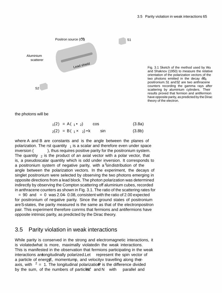
3.5 Parity violation in weak interactions 65
Aluminiumscatterer
S2
S1�Positron source (Cu64)
Lead shieldFig. 3.1 Sketch of the method used by Wuand Shaknov (1950) to measure the relativeorientation of the polarization vectors of thetwo photons emitted in the decay of 1S0positronium. S1 and S2 are two anthracenecounters recording the gamma rays afterscattering by aluminium cylinders. Theirresults proved that fermion and antifermionhave opposite parity, as predicted by the Diractheory of the electron.
the photons will be
ψ1(2γ) = A (ε1 · ε2) ∝ cos φ (3.8a)
ψ2(2γ) = B (ε1 × ε2) · k ∝ sin φ (3.8b)
where A and B are constants and φ is the angle between the planes ofpolarization. The first quantity ψ1 is a scalar and therefore even under spaceinversion (φ → −φ), thus requires positive parity for the positronium system.The quantity ψ2 is the product of an axial vector with a polar vector, thatis, a pseudoscalar quantity which is odd under inversion. It corresponds toa positronium system of negative parity, with a sin2 φ distribution of theangle between the polarization vectors. In the experiment, the decays ofsinglet positronium were selected by observing the two photons emerging inopposite directions from a lead block. The photon polarization was determinedindirectly by observing the Compton scattering off aluminium cubes, recordedin anthracene counters as shown in Fig. 3.1. The ratio of the scattering rates forφ = 90◦ and φ = 0◦ was 2.04±0.08, consistent with the ratio of 2.00 expectedfor positronium of negative parity. Since the ground states of positroniumare S-states, the parity measured is the same as that of the electron–positronpair. This experiment therefore confirms that fermions and antifermions haveopposite intrinsic parity, as predicted by the Dirac theory.
3.5 Parity violation in weak interactions
While parity is conserved in the strong and electromagnetic interactions, itis violated—what is more, maximally violated—in the weak interactions.This is manifested in the observation that fermions participating in the weakinteractions are longitudinally polarized. Let σ represent the spin vector ofa particle of energy E, momentum p, and velocity v travelling along the z-axis, with σ 2 = 1. The longitudinal polarization P is the difference dividedby the sum, of the numbers of particles N+ and N− with σ parallel and
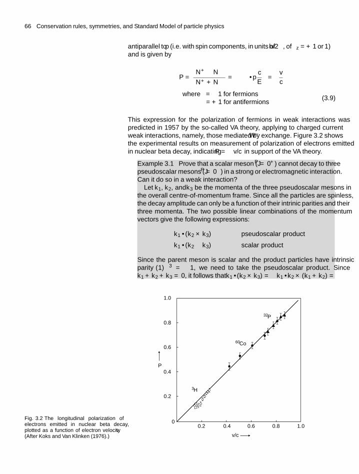
66 Conservation rules, symmetries, and Standard Model of particle physics
antiparallel to p (i.e. with spin components, in units of h/2π, of σz = +1 or −1)and is given by
P =(N+ − N−)(N+ + N−) = α
(σ · p
c
E
)= α
v
c
where α = −1 for fermionsα = +1 for antifermions
(3.9)
This expression for the polarization of fermions in weak interactions waspredicted in 1957 by the so-called V–A theory, applying to ‘charged current’weak interactions, namely, those mediated by W ± exchange. Figure 3.2 showsthe experimental results on measurement of polarization of electrons emittedin nuclear beta decay, indicating P = −v/c in support of the V–A theory.
Example 3.1 Prove that a scalar meson (J P = 0+) cannot decay to threepseudoscalar mesons (J P = 0−) in a strong or electromagnetic interaction.Can it do so in a weak interaction?
Let k1, k2, and k3 be the momenta of the three pseudoscalar mesons inthe overall centre-of-momentum frame. Since all the particles are spinless,the decay amplitude can only be a function of their intrinic parities and theirthree momenta. The two possible linear combinations of the momentumvectors give the following expressions:
k1 · (k2 × k3) pseudoscalar product
k1 · (k2 − k3) scalar product
Since the parent meson is scalar and the product particles have intrinsicparity (−1)3 = −1, we need to take the pseudoscalar product. Sincek1 + k2 + k3 = 0, it follows that k1 · (k2 × k3) = −k1 · k2 × (k1 + k2) =
Fig. 3.2 The longitudinal polarization ofelectrons emitted in nuclear beta decay,plotted as a function of electron velocity v.(After Koks and Van Klinken (1976).)
32P
60Co
3H
00.2 0.4 0.80.6 1.0
P
v/c
–1.0
–0.8
–0.6
–0.4
–0.2
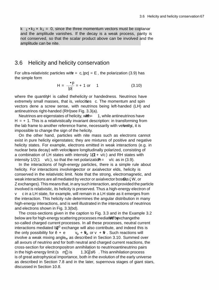
3.6 Helicity and helicity conservation 67
−k1 · k2 × k1 = 0, since the three momentum vectors must be coplanarand the amplitude vanishes. If the decay is a weak process, parity isnot conserved, so that the scalar product above can be involved and theamplitude can be finite.
3.6 Helicity and helicity conservation
For ultra-relativistic particles with v = c, |pc| = E, the polarization (3.9) hasthe simple form
H = σ · p|p| = +1 or − 1 (3.10)
where the quantity H is called the helicity or handedness. Neutrinos haveextremely small masses, that is, velocities v ≈ c. The momentum and spinvectors define a screw sense, with neutrinos being left-handed (LH) andantineutrinos right-handed (RH)—see Fig. 3.3(a).
Neutrinos are eigenstates of helicity, with H = −1, while antineutrinos haveH = +1. This is a relativistically invariant description: in transforming fromthe lab frame to another reference frame, necessarily with velocity v < c, it isimpossible to change the sign of the helicity.
On the other hand, particles with finite mass such as electrons cannotexist in pure helicity eigenstates; they are mixtures of positive and negativehelicity states. For example, electrons emitted in weak interactions (e.g. innuclear beta decay) with velocity v are longitudinally polarized, consisting ofa combination of LH states with intensity 1/2 (1 + v/c) and RH states withintensity 1/2 (1 − v/c), so that the net polarization P = −v/c as in (3.9).
In the interactions of high-energy particles, there is a simple rule abouthelicity. For interactions involving vector or axial–vector fields, helicity isconserved in the relativistic limit. Note that the strong, electromagnetic, andweak interactions are all mediated by vector or axial–vector bosons (G, γ , W , orZ exchanges). This means that, in any such interaction, and provided the particleinvolved is relativistic, its helicity is preserved. Thus a high-energy electron ofv ≈ c in a LH state, for example, will remain in a LH state as it emerges fromthe interaction. This helicity rule determines the angular distribution in manyhigh-energy interactions, and is well illustrated in the interactions of neutrinosand electrons shown in Fig. 3.3(b–d).
The cross-sections given in the caption to Fig. 3.3 and in the Example 3.2below are for high-energy scattering processes mediated by W ± exchange—theso-called ‘charged current’ processes. In all these processes, ‘neutral current’interactions mediated by Z0 exchange will also contribute, and indeed this isthe only possibility for e+ + e− → vμ + vμ or vτ + vτ . Such reactions willinvolve a weak mixing angle θw as described in Section 3.10. Summed overall flavours of neutrino and for both neutral and charged current reactions, thecross-section for electron–positron annihilation to neutrino–antineutrino pairsin the high-energy limit (s � m2
e) is σ ≈ 1.3G2Fs/6π. This annihilation process
is of great astrophysical importance, both in the evolution of the early universeas described in Section 7.8 and in the later, supernova stages of giant stars,discussed in Section 10.8.
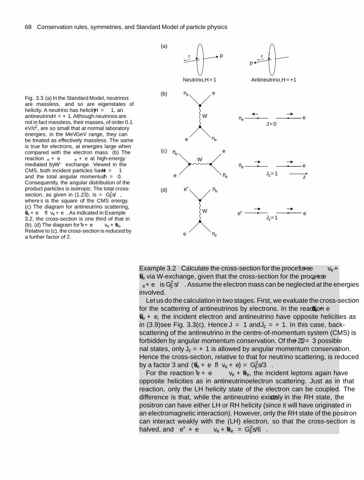
68 Conservation rules, symmetries, and Standard Model of particle physics
Fig. 3.3 (a) In the Standard Model, neutrinosare massless, and so are eigenstates ofhelicity. A neutrino has helicity H = −1, anantineutrino H = +1. Although neutrinos arenot in fact massless, their masses, of order 0.1eV/c2, are so small that at normal laboratoryenergies, in the MeV–GeV range, they canbe treated as effectively massless. The sameis true for electrons, at energies large whencompared with the electron mass. (b) Thereaction νe + e → νe + e at high-energymediated by W ± exchange. Viewed in theCMS, both incident particles have H = −1and the total angular momentum J = 0.Consequently, the angular distribution of theproduct particles is isotropic. The total cross-section, as given in (1.23), is σ = G2
Fs/π,where s is the square of the CMS energy.(c) The diagram for antineutrino scattering,ve + e− → ve + e−. As indicated in Example3.2, the cross-section is one third of that in(b). (d) The diagram for e+ + e− → ve + ve.Relative to (c), the cross-section is reduced bya further factor of 2.
(a)
(b)
(c)
(d)
e
e
e
e
e
e
ne
ne
ne
ne
ne
e–
e–
e+
e+
�z �zpp
Neutrino, H = –1 Antineutrino, H = +1
W
W
W
J = 0
Jz = 1
Jz = 1
z
ne
ne
ne
Example 3.2 Calculate the cross-section for the process e+ +e− → ve +ve via W-exchange, given that the cross-section for the process νe + e− →νe +e− is G2
F s/π. Assume the electron mass can be neglected at the energiesinvolved.
Let us do the calculation in two stages. First, we evaluate the cross-sectionfor the scattering of antineutrinos by electrons. In the reaction ve + e →ve + e, the incident electron and antineutrino have opposite helicities asin (3.9)—see Fig. 3.3(c). Hence J = 1 and Jz = +1. In this case, back-scattering of the antineutrino in the centre-of-momentum system (CMS) isforbidden by angular momentum conservation. Of the 2J + 1 = 3 possiblefinal states, only Jz = +1 is allowed by angular momentum conservation.Hence the cross-section, relative to that for neutrino scattering, is reducedby a factor 3 and σ (ve + e → ve + e) = G2
Fs/3π.For the reaction e+ + e− → ve + ve, the incident leptons again have
opposite helicities as in antineutrino–electron scattering. Just as in thatreaction, only the LH helicity state of the electron can be coupled. Thedifference is that, while the antineutrino exists only in the RH state, thepositron can have either LH or RH helicity (since it will have originated inan electromagnetic interaction). However, only the RH state of the positroncan interact weakly with the (LH) electron, so that the cross-section ishalved, and σ
(e+ + e− → ve + ve
) = G2Fs/6π.
3.7 Charge conjugation invariance 69
3.7 Charge conjugation invariance
The operation of charge conjugation C reverses the sign of the electric chargeand magnetic moment of a particle, leaving all other coordinates unchanged.Both strong and electromagnetic interactions are invariant under the C-operation. For example, Maxwell’s equations are invariant under change of signof the charge or current and thence of the fields E and H. In relativistic quantummechanics, charge conjugation also implies particle–antiparticle conjugation,for example, e− ↔ e+. As an example of particle–antiparticle symmetry inelectromagnetic interactions, a cyclic accelerator can accelerate electrons ina toroidal vacuum tube by means of radio-frequency cavities, and constrainsthem in, say, a clockwise circular path by means of a magnet ring. The samemachine will equally accelerate positrons in an anti-clockwise direction, andthis principle is used in electron–positron colliders, where the accelerated beamswith equal energies are arranged, by means of bending and focusing magnets,to meet head-on once or many times per revolution.
On the contrary, weak interactions are not invariant under C. As shown inFig. 3.3, a neutrino has H = −1, and the C-operation would transform it intoan antineutrino of H = −1, which is a state that does not exist. However, thecombined operation CP—charge conjugation followed by space inversion—would transform a LH neutrino into a RH antineutrino, which does exist (seeSection 3.14 and Fig. 3.14 below).
Of course, to the extent that both lepton number (for the charged leptons)and baryon number are conserved, there can be no physical process turning anelectron into a positron or a proton into an antiproton. However, neutral bosons,which are their own antiparticles, could be eigenstates of the C-operator. Forexample, under the C-operation the wavefunction of a neutral pion transformsinto itself: C
∣∣π0〉 → η∣∣π0〉 where, since repeating the process gets us back to
the original state, η2 = 1 and C∣∣π0〉 = ±∣∣π0〉. The neutral pion decays through
an electromagnetic interaction, π0 → 2γ . The photon must have C = −1since it is generated by charges and currents which reverse sign under the C-operation, and so for a system of n photons, C = (−1)n. Thus the neutral pionmust have C = +1, and the decay π0 → 3γ is forbidden by C-invariance inelectromagnetic interactions.
3.8 Gauge transformations and gauge invariance
In Section 3.1, we described examples of translations and rotations in physicalspace and time. What is just as significant for particle physics are the resultsof ‘internal’ symmetry transformations. For example, the plane wave functionψ representing a particle with four-momentum p(= pμ where μ = 0, 1, 2, 3)can be modified by inserting an arbitrary phase factor α. If x(= xμ) is thespace–time coordinate then the transformation is (in units h = c = 1):
ψ = exp(ipx)→ ψ = exp i
(px + α
)(3.11)
From (3.2) this operation is equivalent to a rotation in some internal ‘chargespace’ of the particle. Clearly, if this phase transformation is global (i.e. thesame over all space), it cannot affect any physical observable. For example,
70 Conservation rules, symmetries, and Standard Model of particle physics
differentiating (3.11), one finds for the expectation value of the momentum ofan electron
−ψ∗i∂ψ
∂x= p (3.12)
where −i∂/∂x is the momentum operator and the asterisk indicates complexconjugation. The result is independent of the choice of α, since the phasefactors cancel. As indicated in Section 3.1, the invariance of the Lagrangiandensity under such a global phase transformation actually leads to a conservedcurrent, via Noether’s theorem. We can illustrate this by writing the abovetransformation as a small increment (α 1):
ψ → ψ (1 + iα) (3.13)
The Lagrangian energy density L of the field ψ appears in the Euler–Lagrangeequation analogous to the classical equation (3.1):
∂
∂x
(∂L
∂ψ′
)− ∂L
∂ψ= 0 (3.14)
where ψ′ = ∂ψ/∂x. If L is invariant under the transformation (3.13), then
δL = 0 = iαψ
(∂L
∂ψ
)+ iαψ′
(∂L
∂ψ′
)and since
iα∂
∂x
(ψ
∂L
∂ψ′
)= iαψ′ ∂L
∂ψ′ + iαψ∂
∂x
(∂L
∂ψ′
)then
δL = 0 = iαψ
(∂L
∂ψ− ∂
∂x
(∂L
∂ψ′
))+ iα
∂
∂x
(ψ
∂L
∂ψ′
)The first term on the right-hand side vanishes, from (3.14), so that the secondterm must also be zero. Thus if we denote the four-current by
J(= Jμ
) = ψ
(∂L
∂ψ′
),
this is conserved:∂J
∂x= 0 (3.15)
From (3.12) and the example of the Lagrangian for a scalar field in (3.25), wecan see that this four-current has the dimensions of a four momentum. If wehad included the electric charge |e| as a factor in the phase transformation, thenthe above equation would represent conservation of electric current. Noticethat in classical mechanics, invariance of the Lagrangian under some operation(e.g. translation in space) leads to a constant of the motion (in this case, theconserved three momentum), while in quantum mechanics, invariance of theLagrangian density—a function of both space and time—under a global phasetransformation leads to a conserved current.
3.8 Gauge transformations and gauge invariance 71
So much for global phase transformations. However, it is also possibleto make a local phase transformation, that is, one for which α = α(x) is afunction of the space/time coordinate. Then, including a factor |e| in the phaseto emphasize that we are dealing with electric currents
∂ψ
∂x= i
(p + e
∂α
∂x
)ψ
In this case, physically observable quantities like momentum will be affectedby the choice of α and its x-dependence, so local phase invariance does notappear to be a useful concept. However, the electron is a charged particle andwill therefore be subject to any electromagnetic potential, which will comprisea vector potential A and a scalar potential �. We know that the effect of � isto change the energy of the particle from E to E − e�, and correspondingly,the four-vector potential A = (A, �) will change the four-momentum from pto (p − eA). Hence, if one includes the effects of an electromagnetic potentialof arbitrary magnitude, the above derivative becomes
∂ψ
∂x= i
(p − eA + e
∂α
∂x
)ψ (3.16)
The scale or gauge of the potential A is also arbitrary: one can add to it thegradient of any scalar function, without affecting the values of any physicallymeasurable quantities, namely, the associated electric and magnetic fields. Thischange of the scale or gauge of the potential is called a gauge transformation.Choosing α as this arbitrary scalar function, the transformation A → A+∂α/∂xgives for the derivative
∂ψ
∂x→ i
(p − eA − e
∂α
∂x+ e
∂α
∂x
)ψ = i
(p − eA
)ψ (3.17)
so that an observable quantity such as ψ∗∂ψ/∂x no longer contains α or ∂α/∂x.The quantity ∂/∂x on the left-hand side has thus been replaced by i(p − eA) or,in operator notation
∂
∂x→ D = ∂
∂x− ieA (3.18)
called the covariant derivative. Note that x and A here are four-vector quantities,that is the space–time coordinate x = xμ(μ = 0, 1, 2, 3 with x0 = ct, x1 = x,x2 = y, x3 = z), and similarly for the four-vector potential A = Aμ, so thatwhen written with the indices (3.18) becomes
D = ∂
∂xμ
− ieAμ (3.19)
In summary, by judicious choice of the scalar function the effects of theoriginal local phase transformation on the electron wavefunction and the gaugetransformation on the potential cancel exactly. The fact that it is possibleto formulate the theoretical description to have this property of local gaugeinvariance turns out to be vital for the quantum field theory of electromagnetism,called quantum electrodynamics (QED).
Intuitively, one can see on a qualitative basis that these global and localinvariances must be consistent with charge conservation and the masslessness
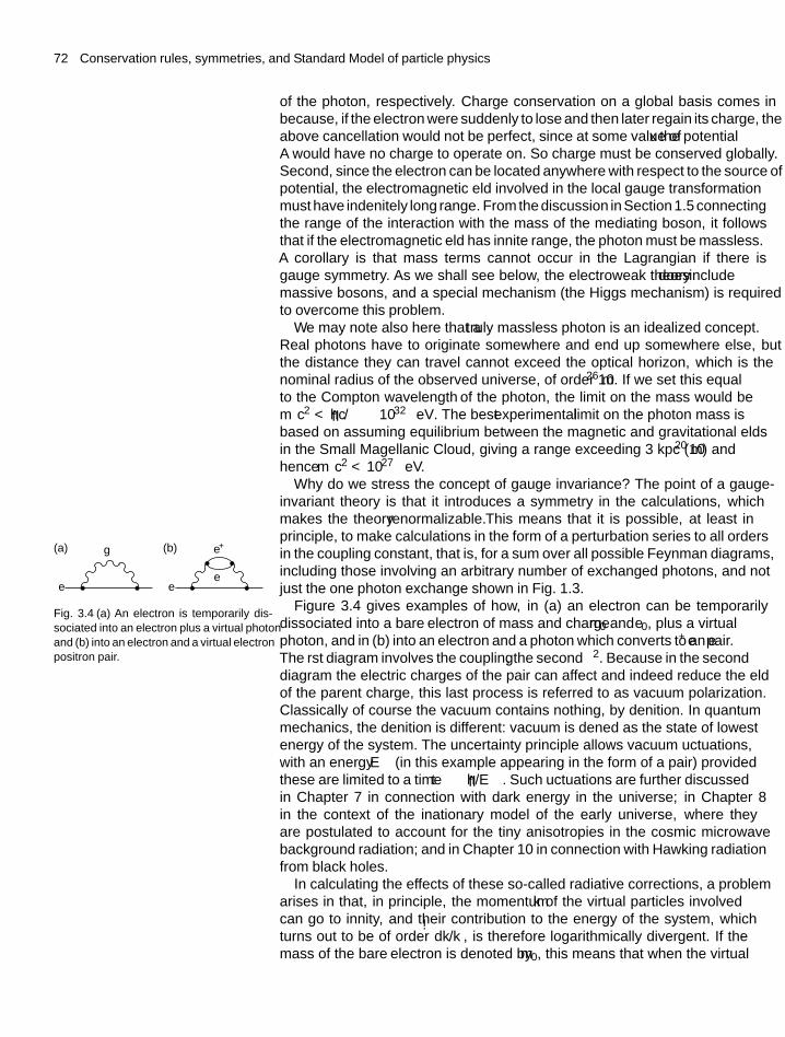
72 Conservation rules, symmetries, and Standard Model of particle physics
of the photon, respectively. Charge conservation on a global basis comes inbecause, if the electron were suddenly to lose and then later regain its charge, theabove cancellation would not be perfect, since at some value of x the potentialA would have no charge to operate on. So charge must be conserved globally.Second, since the electron can be located anywhere with respect to the source ofpotential, the electromagnetic field involved in the local gauge transformationmust have indefinitely long range. From the discussion in Section 1.5 connectingthe range of the interaction with the mass of the mediating boson, it followsthat if the electromagnetic field has infinite range, the photon must be massless.A corollary is that mass terms cannot occur in the Lagrangian if there isgauge symmetry. As we shall see below, the electroweak theory does includemassive bosons, and a special mechanism (the Higgs mechanism) is requiredto overcome this problem.
We may note also here that a truly massless photon is an idealized concept.Real photons have to originate somewhere and end up somewhere else, butthe distance they can travel cannot exceed the optical horizon, which is thenominal radius of the observed universe, of order 1026 m. If we set this equalto the Compton wavelength λ of the photon, the limit on the mass would bemγc2 < hc/λ ∼ 10−32 eV. The best experimental limit on the photon mass isbased on assuming equilibrium between the magnetic and gravitational fieldsin the Small Magellanic Cloud, giving a range exceeding 3 kpc (1020 m) andhence mγc2 < 10−27 eV.
Why do we stress the concept of gauge invariance? The point of a gauge-invariant theory is that it introduces a symmetry in the calculations, whichmakes the theory renormalizable. This means that it is possible, at least inprinciple, to make calculations in the form of a perturbation series to all ordersin the coupling constant, that is, for a sum over all possible Feynman diagrams,including those involving an arbitrary number of exchanged photons, and notjust the one photon exchange shown in Fig. 1.3.
e+
ee
(a) (b)g
e–
Fig. 3.4 (a) An electron is temporarily dis-sociated into an electron plus a virtual photonand (b) into an electron and a virtual electron–positron pair.
Figure 3.4 gives examples of how, in (a) an electron can be temporarilydissociated into a ‘bare’ electron of mass and charge m0 and e0, plus a virtualphoton, and in (b) into an electron and a photon which converts to an e+e− pair.The first diagram involves the coupling α, the second α2. Because in the seconddiagram the electric charges of the pair can affect and indeed reduce the fieldof the parent charge, this last process is referred to as ‘vacuum polarization’.Classically of course the vacuum contains nothing, by definition. In quantummechanics, the definition is different: vacuum is defined as the state of lowestenergy of the system. The uncertainty principle allows ‘vacuum fluctuations’,with an energy �E (in this example appearing in the form of a pair) providedthese are limited to a time �t ∼ h/�E. Such fluctuations are further discussedin Chapter 7 in connection with dark energy in the universe; in Chapter 8in the context of the inflationary model of the early universe, where theyare postulated to account for the tiny anisotropies in the cosmic microwavebackground radiation; and in Chapter 10 in connection with Hawking radiationfrom black holes.
In calculating the effects of these so-called radiative corrections, a problemarises in that, in principle, the momentum k of the virtual particles involvedcan go to infinity, and their contribution to the energy of the system, whichturns out to be of order
∫dk/k, is therefore logarithmically divergent. If the
mass of the ‘bare’ electron is denoted by m0, this means that when the virtual
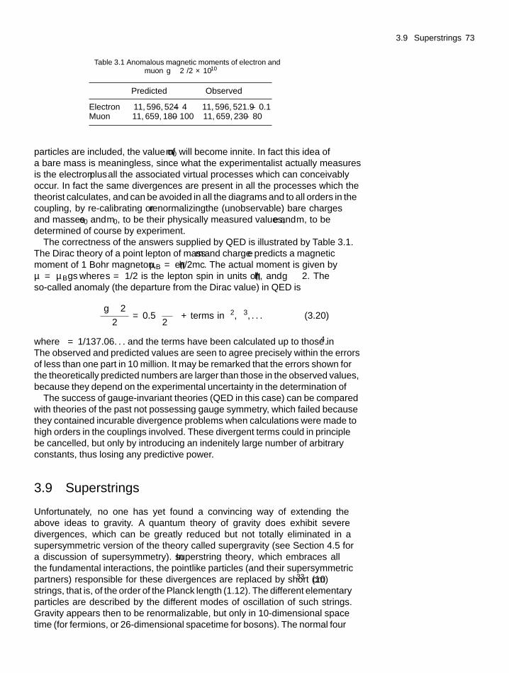
3.9 Superstrings 73
Table 3.1 Anomalous magnetic moments of electron andmuon
(g − 2
)/2 × 1010
Predicted Observed
Electron 11, 596, 524 ± 4 11, 596, 521.9 ± 0.1Muon 11, 659, 180±100 11, 659, 230 ± 80
particles are included, the value of m0 will become infinite. In fact this idea ofa bare mass is meaningless, since what the experimentalist actually measuresis the electron plus all the associated virtual processes which can conceivablyoccur. In fact the same divergences are present in all the processes which thetheorist calculates, and can be avoided in all the diagrams and to all orders in thecoupling, by re-calibrating or renormalizing the (unobservable) bare chargesand masses e0 and m0, to be their physically measured values, e and m, to bedetermined of course by experiment.
The correctness of the answers supplied by QED is illustrated by Table 3.1.The Dirac theory of a point lepton of mass m and charge e predicts a magneticmoment of 1 Bohr magneton, μB = eh/2mc. The actual moment is given byμ = μBgs where s = 1/2 is the lepton spin in units of h, and g ≈ 2. Theso-called anomaly (the departure from the Dirac value) in QED is(
g − 2)
2= 0.5
( α
2π
)+ terms in α2, α3, . . . (3.20)
where α = 1/137.06 . . . and the terms have been calculated up to those in α4.The observed and predicted values are seen to agree precisely within the errorsof less than one part in 10 million. It may be remarked that the errors shown forthe theoretically predicted numbers are larger than those in the observed values,because they depend on the experimental uncertainty in the determination of α.
The success of gauge-invariant theories (QED in this case) can be comparedwith theories of the past not possessing gauge symmetry, which failed becausethey contained incurable divergence problems when calculations were made tohigh orders in the couplings involved. These divergent terms could in principlebe cancelled, but only by introducing an indefinitely large number of arbitraryconstants, thus losing any predictive power.
3.9 Superstrings
Unfortunately, no one has yet found a convincing way of extending theabove ideas to gravity. A quantum theory of gravity does exhibit severedivergences, which can be greatly reduced but not totally eliminated in asupersymmetric version of the theory called supergravity (see Section 4.5 fora discussion of supersymmetry). In superstring theory, which embraces allthe fundamental interactions, the pointlike particles (and their supersymmetricpartners) responsible for these divergences are replaced by short (10−33 cm)strings, that is, of the order of the Planck length (1.12). The different elementaryparticles are described by the different modes of oscillation of such strings.Gravity appears then to be renormalizable, but only in 10-dimensional space–time (for fermions, or 26-dimensional space–time for bosons). The normal four
74 Conservation rules, symmetries, and Standard Model of particle physics
dimensions of space and time we actually observe will result if all the extradimensions are ‘curled up’ into the tiny extent of the string length, accordingto the original ideas of Kaluza and Klein in the 1920s. The weakness of thegravitational force is then ascribed to the fact that at normal energies, these extradimensions are ineffective, and it is only when one reaches energies of the orderof the Planck energy (or lengths comparable with the Planck length) that gravitybecomes strong. Superstring theory does correctly predict the spin 2 of thegraviton. Unfortunately, it also predicts a massive superpartner, the gravitinoof spin 3/2. If this were produced, like the other elementary particles, in thehot early universe, its decay products would completely alter the predictionson nucleosynthesis of the light elements and ruin the close agreement withexperiment, as described in Chapter 6. In summary, incorporating gravity withthe other interactions is still an unsolved problem.
3.10 Gauge invariance in the electroweak theory
In QED, we saw that gauge invariance is associated with an infinite set of phasetransformations of the wavefunction of the form
ψ → ψ exp [ieα (x)] (3.21)
These transformations are actually elements of a group called U(1), the ‘U’standing for unitary, implying that the norm of the wavefunction is preservedin the transformation, and the ‘1’ that it refers to a rotation in one dimension.In the electroweak theory, more complicated transformations, belonging to theSU(2) group are also involved. They are of the form,
ψ → ψ exp [igτ · �] (3.22)
Here the transformation involves the Pauli 2 × 2 matrices τ = (τ1, τ2, τ3)
and describes rotations about the arbitrary vector �. The Pauli matrices wereoriginally invented to describe spin 1/2 particles, the ‘2’ in the nomenclatureSU(2) referring to the dimension of the matrices, the ‘U’ indicating that thetransformation is again unitary. The ‘S’ stands for ‘special’, SU(2) being asubgroup of U(2) in which the matrices are traceless. A fundamental differencebetween the transformations (3.21) and (3.22) is that U(1) is an Abelian groupsince α(x) is a scalar quantity. Thus the effect of two rotations in successionis independent of the order and α1α2 − α2α1 = 0, that is, the two operationscommute. On the other hand, the group SU(2) is non-Abelian, involving thenon-commuting Pauli operators, for example, τ1τ2 − τ2τ1 = iτ3.
The electroweak model was introduced by Glashow (1961), Weinberg(1967), and Salam (1967). It postulates four massless vector bosons; a tripletw+, w− and w0 belonging to the SU(2) group and b0 belonging to the U(1)group, that is, a system with SU(2) × U(1) symmetry. The neutral componentw0 mixes with the b0, to form the photon γ and a neutral boson z0, involvingan arbitrary mixing angle θW . Finally, scalar bosons called Higgs scalars(after their inventor, Higgs (1964)) are postulated, to generate mass by self-interaction, as described below. Three of the four Higgs components areabsorbed by the states w+, w−, and z0, to form the massive vector bosonsW +, W −, and Z0 introduced in Chapter 1, while the photon γ remains massless.
3.11 Higgs mechanism of spontaneous symmetry breaking 75
Furthermore, although massive bosons are involved, the theory does remainrenormalizable. The weak and electromagnetic interactions are unified, andthe coupling of the W to leptons, specified by the coupling constant g in (3.22),is given by the relation e = g sin θW . (There are several numerical factorsentering in the definition of g, which have arisen historically. The quantity gw,which we introduced in (1.9) as g2
w = GF M 2W , is related to g by g2
w = √2g2/8).
The two unknown parameters in the model are the photon mass (zero) which hasto be put in ‘by hand’, and the above mixing angle, which has been measuredas sin2 θW = 0.231 ± 0.001. The boson masses are then predicted in terms ofthe Fermi weak interaction constant GF , e, and the mixing angle:
MW =[
g2
√2
(8GF)
]1/2
=⎡⎣e2
√2(
8GF sin2 θW
)⎤⎦1/2
= 37.4
sin θWGeV
MZ = MW
cos θW(3.23)
The electroweak theory was vindicated by the discovery in 1973 of neutralweak currents, that is, the existence of Z0 exchange as in Fig. 1.3, and bythe observation of the W and Z bosons in 1983 (see Figs. 1.6 and 1.13).Note that, because the W and Z bosons are massive, compared with the zeromass of the photon, the SU(2) × U(1) symmetry of the model is broken bythe Higgs mechanism of mass generation, but because the theory remainsrenormalizable, cross-sections and decay rates mediated by the bosons W andZ can be calculated exactly. All that is missing at the present time is the fourthHiggs component, which should exist as a physical particle. A lower limit onthe mass is MH > 100 GeV. Finding the elusive Higgs is one of the primeobjectives of experimental high-energy physics at the present time.
3.11 The Higgs mechanism of spontaneoussymmetry breaking
We now discuss briefly the Higgs mechanism for spontaneous symmetrybreaking in the electroweak theory. It is relevant to introduce it here, not onlybecause it is an intrinsic part of the very successful electroweak theory, but alsobecause a somewhat similar mechanism has been postulated in connection withthe inflationary model of the early universe, which is discussed in Chapter 8.
As stated in Section 3.1, the equation for the Lagrangian energy density L ofa field � in a quantum-mechanical system is written as
∂
∂xμ
(∂L
∂�′
)− ∂L
∂�= 0 (3.24)
where �′ = ∂�/∂xμ, � is the amplitude of the field particles and xμ (withμ = 0, 1, 2, 3) is the space–time coordinate (so in units h = c = 1, x0 =t, x1 = x, x2 = y, and x3 = z). For free scalar particles of mass μ the Lagrangian
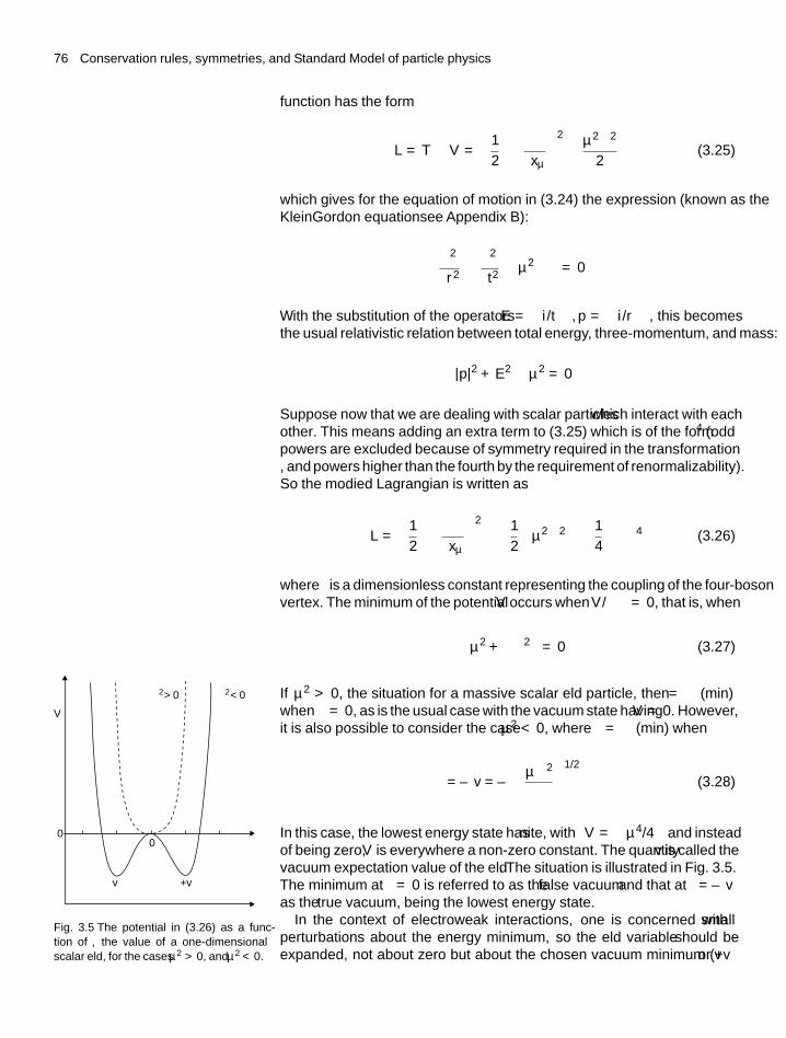
76 Conservation rules, symmetries, and Standard Model of particle physics
function has the form
L = T − V =(
1
2
)(∂�
∂xμ
)2
− μ2�2
2(3.25)
which gives for the equation of motion in (3.24) the expression (known as theKlein–Gordon equation—see Appendix B):
(∂2
∂r2− ∂2
∂t2− μ2
)� = 0
With the substitution of the operators E = −i∂/∂t, p = −i∂/∂r, this becomesthe usual relativistic relation between total energy, three-momentum, and mass:
− |p|2 + E2 − μ2 = 0
Suppose now that we are dealing with scalar particles which interact with eachother. This means adding an extra term to (3.25) which is of the form �4 (oddpowers are excluded because of symmetry required in the transformation � →−�, and powers higher than the fourth by the requirement of renormalizability).So the modified Lagrangian is written as
L =(
1
2
)(∂�
∂xμ
)2
−(
1
2
)μ2�2 −
(1
4
)λ�4 (3.26)
where λ is a dimensionless constant representing the coupling of the four-bosonvertex. The minimum of the potential V occurs when ∂V /∂� = 0, that is, when
�(μ2 + λ�2
)= 0 (3.27)
If μ2 > 0, the situation for a massive scalar field particle, then � = � (min)when � = 0, as is the usual case with the vacuum state having V = 0. However,it is also possible to consider the case μ2 < 0, where � = � (min) when
� = ±v = ±(−μ2
λ
)1/2
(3.28)
In this case, the lowest energy state has � finite, with V = −μ4/4λ and insteadof being zero, V is everywhere a non-zero constant. The quantity v is called thevacuum expectation value of the field �. The situation is illustrated in Fig. 3.5.The minimum at � = 0 is referred to as the false vacuum and that at � = ±vas the true vacuum, being the lowest energy state.
V
00
�
–v +v
�2 > 0 �2 < 0
Fig. 3.5 The potential in (3.26) as a func-tion of �, the value of a one-dimensionalscalar field, for the cases μ2 > 0, and μ2 < 0.
In the context of electroweak interactions, one is concerned with smallperturbations about the energy minimum, so the field variable � should beexpanded, not about zero but about the chosen vacuum minimum (+v or −v
3.12 Running couplings 77
in the above example). If one writes
� = v + σ (x) (3.29)
where σ is the value of the extra field over and above the constant and uniformvalue v, then substituting into (3.25) one gets
L =(
1
2
)(∂σ
∂xμ
)2
− λv2σ2 −(
λvσ3 + λσ4
4
)+ constant (3.30)
where the constant terms involve powers of v only. The third term representsthe interaction of the σ field with itself. The second term, when compared withthe potential in (3.26), is clearly a mass term, with a value for the mass of
m =√
2λv2 =√
−2μ2 (3.31)
So, by making a perturbation expansion about either of the minima +v or −v,a positive real mass has appeared. Note that the expansion has to be madeabout one of the two minima. Of course, once this is done, the symmetry ofFig. 3.5 is broken. Such a behaviour is called spontaneous symmetry breaking.Many examples exist in physics. A bar magnet heated above the Curie pointhas its elementary magnetic domains pointed in random directions, with zeronet moment, and the Lagrangian is invariant under rotations of the magnet inspace. On cooling, the domains will set in one particular direction, that of theresultant moment, and the rotational symmetry is spontaneously broken.
The treatment above was of a one-component scalar field. For the moregeneral case of a complex scalar field, �1 + i�2, the two points ±v in Fig. 3.5are replaced by all the points on a circle of radius v obtained by rotating thediagram about a vertical axis. However, the principle of obtaining a real massassociated with the lowest energy ‘true’vacuum state by spontaneously breakingthe symmetry of the potential remains as before.
The next step is to replace the derivative ∂/∂xμ in (3.30) by the covariantderivative analogous to that in (3.19) but extended to include both the U(1)and SU(2) transformations in (3.21) and (3.22). When this is done, one obtainsrelations for the squares of the masses of the W and Z bosons as in (3.23), andalso in terms of the Higgs vacuum term v. The measured values of the bosonmasses give v = 246 GeV, which is thus the scale of the electroweak symmetrybreaking. However, the Higgs mass is not directly predicted by the theory, butit should have a mass of the order of the electroweak scale and in any case lessthan 1 TeV.
3.12 Running couplings: comparison ofelectroweak theory and quantumchromodynamics with experiment
In Section 3.8 it was noted that in gauge theories, perturbation calculationsgiving finite answers can be carried out to any order in the coupling constant.However, there is a practical limit. For example, in calculating the (g − 2)correction to the electron magnetic moment, there are already 72 Feynman
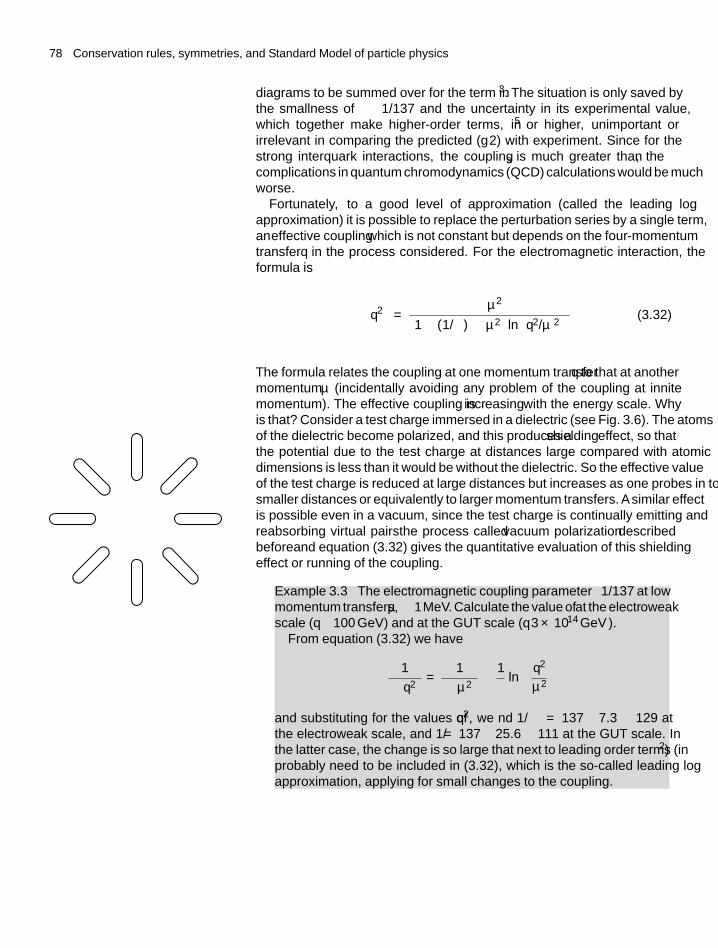
78 Conservation rules, symmetries, and Standard Model of particle physics
diagrams to be summed over for the term in α3. The situation is only saved bythe smallness of α ∼ 1/137 and the uncertainty in its experimental value,which together make higher-order terms, in α5 or higher, unimportant orirrelevant in comparing the predicted (g − 2) with experiment. Since for thestrong interquark interactions, the coupling αs is much greater than α, thecomplications in quantum chromodynamics (QCD) calculations would be muchworse.
Fortunately, to a good level of approximation (called the leading logapproximation) it is possible to replace the perturbation series by a single term,an effective coupling which is not constant but depends on the four-momentumtransfer q in the process considered. For the electromagnetic interaction, theformula is
α(
q2)
= α(μ2)[
1 − (1/π) α(μ2)
ln(q2/μ2
)] (3.32)
The formula relates the coupling at one momentum transfer q to that at anothermomentum μ (incidentally avoiding any problem of the coupling at infinitemomentum). The effective coupling is increasing with the energy scale. Whyis that? Consider a test charge immersed in a dielectric (see Fig. 3.6). The atomsof the dielectric become polarized, and this produces a shielding effect, so thatthe potential due to the test charge at distances large compared with atomicdimensions is less than it would be without the dielectric. So the effective valueof the test charge is reduced at large distances but increases as one probes in tosmaller distances or equivalently to larger momentum transfers. Asimilar effectis possible even in a vacuum, since the test charge is continually emitting andreabsorbing virtual pairs—the process called vacuum polarization describedbefore—and equation (3.32) gives the quantitative evaluation of this shieldingeffect or running of the coupling.
Example 3.3 The electromagnetic coupling parameter α ≈ 1/137 at lowmomentum transfers, μ ∼ 1 MeV. Calculate the value of αat the electroweakscale (q ∼ 100 GeV) and at the GUT scale (q ∼ 3 × 10¹⁴ GeV ).
From equation (3.32) we have
1
α(q2) = 1
α(μ2) − 1
πln
(q2
μ2
)and substituting for the values of q2, we find 1/α = 137 − 7.3 ∼ 129 atthe electroweak scale, and 1/α = 137 − 25.6 ∼ 111 at the GUT scale. Inthe latter case, the change is so large that next to leading order terms (in α2)probably need to be included in (3.32), which is the so-called leading logapproximation, applying for small changes to the coupling.
+
+ +
+ +
+
+
–
–
– –
– –
+ – – +
Fig. 3.6
For strong interactions (QCD) it turns out that, in addition to the shieldingeffect of fermion (quark) loops there is also an anti-shielding effect, because ofthe loops containing gluons and the (longitudinal component of) gluon–gluoncoupling as shown in Fig. 3.7. This coupling increasingly ‘spreads’ the strongcolour charge at the larger values of q2. In this case, the dependence of the
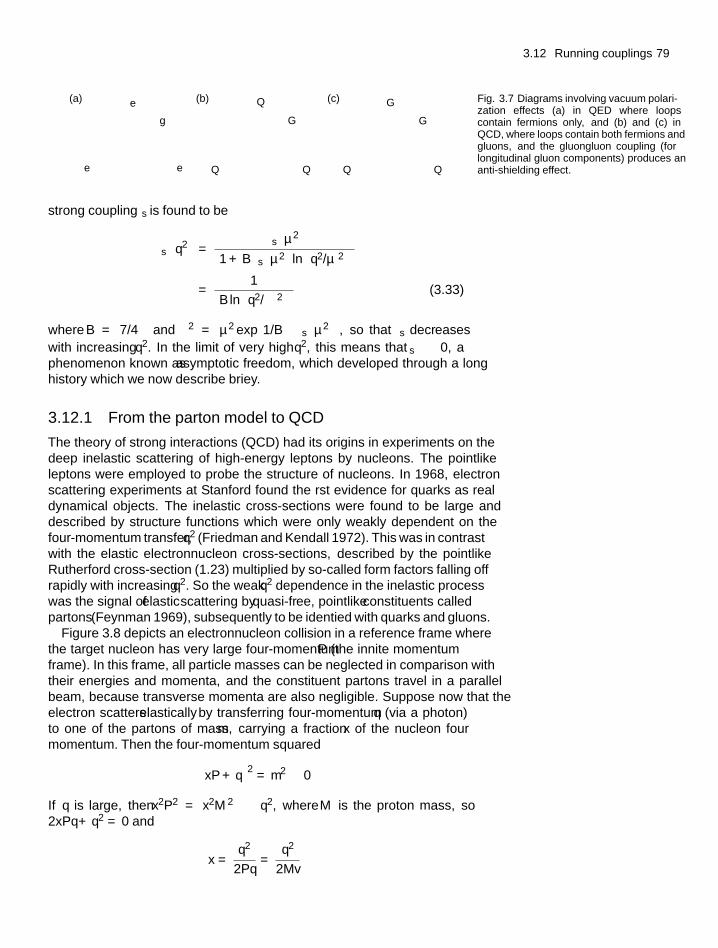
3.12 Running couplings 79
e
e e Q Q Q Q
Q
G
G
Gg
(a) (b) (c) Fig. 3.7 Diagrams involving vacuum polari-zation effects (a) in QED where loopscontain fermions only, and (b) and (c) inQCD, where loops contain both fermions andgluons, and the gluon–gluon coupling (forlongitudinal gluon components) produces ananti-shielding effect.
strong coupling αs is found to be
αs
(q2)
= αs(μ2)[
1 + Bαs(μ2)
ln(q2/μ2
)]= 1[
B ln(q2/�2
)] (3.33)
where B = 7/4π and �2 = μ2 exp[−1/Bαs
(μ2)]
, so that αs decreaseswith increasing q2. In the limit of very high q2, this means that αs → 0, aphenomenon known as asymptotic freedom, which developed through a longhistory which we now describe briefly.
3.12.1 From the parton model to QCD
The theory of strong interactions (QCD) had its origins in experiments on thedeep inelastic scattering of high-energy leptons by nucleons. The pointlikeleptons were employed to probe the structure of nucleons. In 1968, electronscattering experiments at Stanford found the first evidence for quarks as realdynamical objects. The inelastic cross-sections were found to be large anddescribed by structure functions which were only weakly dependent on thefour-momentum transfer, q2 (Friedman and Kendall 1972). This was in contrastwith the elastic electron–nucleon cross-sections, described by the pointlikeRutherford cross-section (1.23) multiplied by so-called form factors falling offrapidly with increasing q2. So the weak q2 dependence in the inelastic processwas the signal of elastic scattering by quasi-free, pointlike constituents calledpartons (Feynman 1969), subsequently to be identified with quarks and gluons.
Figure 3.8 depicts an electron–nucleon collision in a reference frame wherethe target nucleon has very large four-momentum P (the ‘infinite momentumframe’). In this frame, all particle masses can be neglected in comparison withtheir energies and momenta, and the constituent partons travel in a parallelbeam, because transverse momenta are also negligible. Suppose now that theelectron scatters elastically by transferring four-momentum q (via a photon)to one of the partons of mass m, carrying a fraction x of the nucleon fourmomentum. Then the four-momentum squared(
xP + q)2 = m2 ≈ 0
If q is large, then x2P2 = x2M 2 q2, where M is the proton mass, so2xPq + q2 = 0 and
x =∣∣q2∣∣
2Pq=∣∣q2∣∣
2Mv
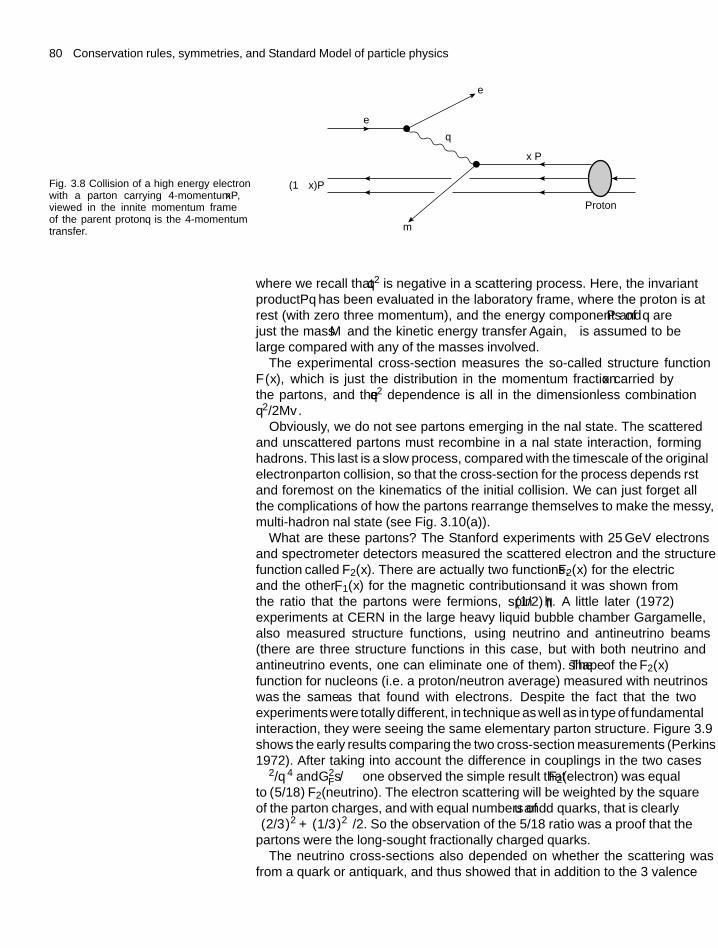
80 Conservation rules, symmetries, and Standard Model of particle physics
Fig. 3.8 Collision of a high energy electronwith a parton carrying 4-momentum xP,viewed in the “infinite momentum frame”of the parent proton. q is the 4-momentumtransfer.
e
q
e
m
x P
Proton
(1 – x)P
where we recall that q2 is negative in a scattering process. Here, the invariantproduct Pq has been evaluated in the laboratory frame, where the proton is atrest (with zero three momentum), and the energy components of P and q arejust the mass M and the kinetic energy transfer ν. Again, ν is assumed to belarge compared with any of the masses involved.
The experimental cross-section measures the so-called structure functionF(x), which is just the distribution in the momentum fraction x carried bythe partons, and the q2 dependence is all in the dimensionless combinationq2/2Mv.
Obviously, we do not see partons emerging in the final state. The scatteredand unscattered partons must recombine in a final state interaction, forminghadrons. This last is a slow process, compared with the timescale of the originalelectron–parton collision, so that the cross-section for the process depends firstand foremost on the kinematics of the initial collision. We can just forget allthe complications of how the partons rearrange themselves to make the messy,multi-hadron final state (see Fig. 3.10(a)).
What are these partons? The Stanford experiments with 25 GeV electronsand spectrometer detectors measured the scattered electron and the ‘structurefunction’ called F2(x). There are actually two functions, F2(x) for the electricand the other, F1(x) for the magnetic contributions—and it was shown fromthe ratio that the partons were fermions, spin (1/2)h. A little later (1972)experiments at CERN in the large heavy liquid bubble chamber Gargamelle,also measured structure functions, using neutrino and antineutrino beams(there are three structure functions in this case, but with both neutrino andantineutrino events, one can eliminate one of them). The shape of the F2(x)function for nucleons (i.e. a proton/neutron average) measured with neutrinoswas the same as that found with electrons. Despite the fact that the twoexperiments were totally different, in technique as well as in type of fundamentalinteraction, they were seeing the same elementary parton structure. Figure 3.9shows the early results comparing the two cross-section measurements (Perkins1972). After taking into account the difference in couplings in the two cases(α2/q4 and G2
Fs/π)
one observed the simple result that F2(electron) was equalto (5/18) F2(neutrino). The electron scattering will be weighted by the squareof the parton charges, and with equal numbers of u and d quarks, that is clearly[(2/3)2 + (1/3)2]/2. So the observation of the 5/18 ratio was a proof that the
partons were the long-sought fractionally charged quarks.The neutrino cross-sections also depended on whether the scattering was
from a quark or antiquark, and thus showed that in addition to the 3 ‘valence’
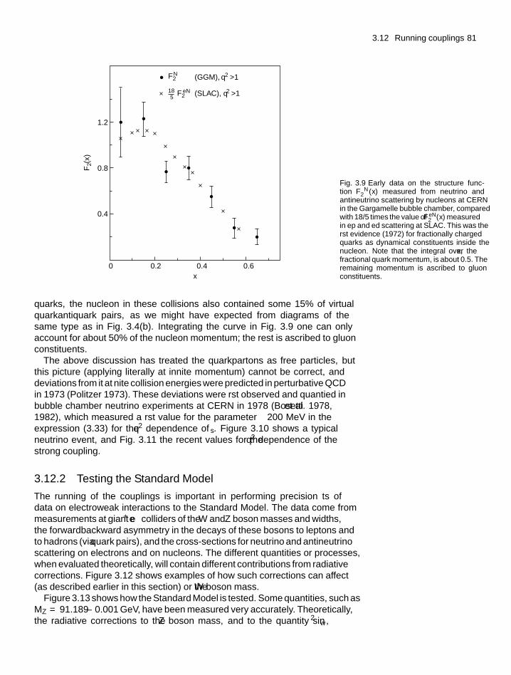
3.12 Running couplings 81
F2(
x)
1.2
185
(GGM), q2 >1
(SLAC), q2 >1
0.8
0.4
0 0.2 0.4 0.6x
F2�N
F2eN
Fig. 3.9 Early data on the structure func-tion FνN
2 (x) measured from neutrino andantineutrino scattering by nucleons at CERNin the Gargamelle bubble chamber, comparedwith 18/5 times the value of FeN
2 (x) measuredin ep and ed scattering at SLAC. This was thefirst evidence (1972) for fractionally chargedquarks as dynamical constituents inside thenucleon. Note that the integral over x, thefractional quark momentum, is about 0.5. Theremaining momentum is ascribed to gluonconstituents.
quarks, the nucleon in these collisions also contained some 15% of virtualquark–antiquark pairs, as we might have expected from diagrams of thesame type as in Fig. 3.4(b). Integrating the curve in Fig. 3.9 one can onlyaccount for about 50% of the nucleon momentum; the rest is ascribed to gluonconstituents.
The above discussion has treated the quark–partons as free particles, butthis picture (applying literally at infinite momentum) cannot be correct, anddeviations from it at finite collision energies were predicted in perturbative QCDin 1973 (Politzer 1973). These deviations were first observed and quantified inbubble chamber neutrino experiments at CERN in 1978 (Bosetti et al. 1978,1982), which measured a first value for the parameter � ∼ 200 MeV in theexpression (3.33) for the q2 dependence of αs. Figure 3.10 shows a typicalneutrino event, and Fig. 3.11 the recent values for the q2 dependence of thestrong coupling.
3.12.2 Testing the Standard Model
The running of the couplings is important in performing precision fits ofdata on electroweak interactions to the Standard Model. The data come frommeasurements at giant e+e− colliders of the W and Z boson masses and widths,the forward–backward asymmetry in the decays of these bosons to leptons andto hadrons (via quark pairs), and the cross-sections for neutrino and antineutrinoscattering on electrons and on nucleons. The different quantities or processes,when evaluated theoretically, will contain different contributions from radiativecorrections. Figure 3.12 shows examples of how such corrections can affect α
(as described earlier in this section) or the W boson mass.Figure 3.13 shows how the Standard Model is tested. Some quantities, such as
MZ = 91.189±0.001 GeV, have been measured very accurately. Theoretically,the radiative corrections to the Z boson mass, and to the quantity sin2 θw,
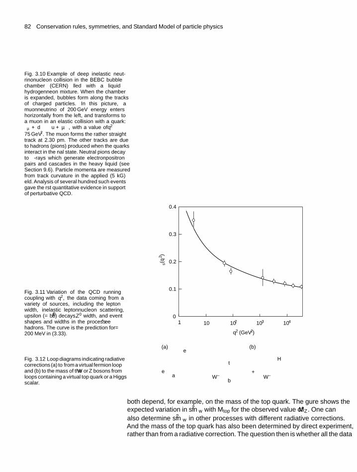
82 Conservation rules, symmetries, and Standard Model of particle physics
Fig. 3.10 Example of deep inelastic neut-rino–nucleon collision in the BEBC bubblechamber (CERN) filled with a liquidhydrogen–neon mixture. When the chamberis expanded, bubbles form along the tracksof charged particles. In this picture, amuon–neutrino of 200 GeV energy entershorizontally from the left, and transforms toa muon in an elastic collision with a quark:νμ + d → u + μ−, with a value of q2 ≈75 GeV2. The muon forms the rather straighttrack at 2.30 pm. The other tracks are dueto hadrons (pions) produced when the quarksinteract in the final state. Neutral pions decayto γ-rays which generate electron–positronpairs and cascades in the heavy liquid (seeSection 9.6). Particle momenta are measuredfrom track curvature in the applied (5 kG)field. Analysis of several hundred such eventsgave the first quantitative evidence in supportof perturbative QCD.
Fig. 3.11 Variation of the QCD ‘runningcoupling’ with q2, the data coming from avariety of sources, including the τ leptonwidth, inelastic lepton–nucleon scattering,upsilon (= bb) decays, Z0 width, and eventshapes and widths in the process e+e− →hadrons. The curve is the prediction for � =200 MeV in (3.33).
� s(q
2 )
q2 (GeV2)
1 10 102 103 104
0.4
0.3
0.2
0.1
0
Fig. 3.12 Loop diagrams indicating radiativecorrections (a) toα from a virtual fermion loopand (b) to the mass of the W or Z bosons fromloops containing a virtual top quark or a Higgsscalar.
e
t
b
+
H
W ±W ±e
a
(a) (b)
both depend, for example, on the mass of the top quark. The figure shows theexpected variation in sin2 θw with Mtop for the observed value of MZ . One canalso determine sin2 θw in other processes with different radiative corrections.And the mass of the top quark has also been determined by direct experiment,rather than from a radiative correction. The question then is whether all the data
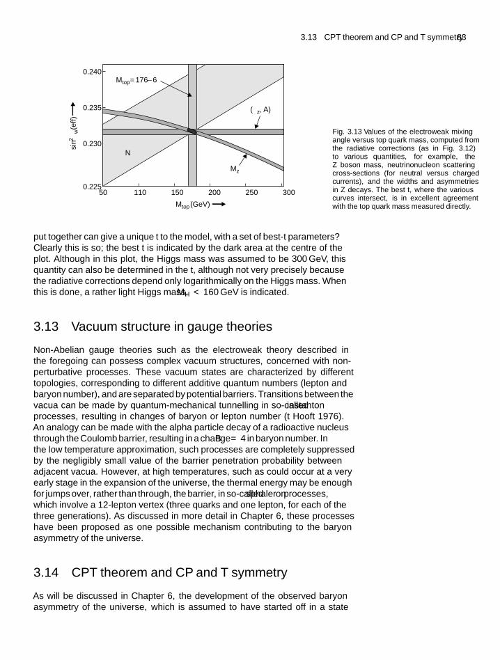
3.13 CPT theorem and CP and T symmetry 83
Mtop = 176 ± 60.240
0.235
0.230
0.22550 110 150 200 250 300
Mtop (GeV)
Mz
N
(z, A)
sin2
� w(e
ff)
Fig. 3.13 Values of the electroweak mixingangle versus top quark mass, computed fromthe radiative corrections (as in Fig. 3.12)to various quantities, for example, theZ boson mass, neutrino–nucleon scatteringcross-sections (for neutral versus chargedcurrents), and the widths and asymmetriesin Z decays. The best fit, where the variouscurves intersect, is in excellent agreementwith the top quark mass measured directly.
put together can give a unique fit to the model, with a set of best-fit parameters?Clearly this is so; the best fit is indicated by the dark area at the centre of theplot. Although in this plot, the Higgs mass was assumed to be 300 GeV, thisquantity can also be determined in the fit, although not very precisely becausethe radiative corrections depend only logarithmically on the Higgs mass. Whenthis is done, a rather light Higgs mass, MH < 160 GeV is indicated.
3.13 Vacuum structure in gauge theories
Non-Abelian gauge theories such as the electroweak theory described inthe foregoing can possess complex vacuum structures, concerned with non-perturbative processes. These vacuum states are characterized by differenttopologies, corresponding to different additive quantum numbers (lepton andbaryon number), and are separated by potential barriers. Transitions between thevacua can be made by quantum-mechanical tunnelling in so-called instantonprocesses, resulting in changes of baryon or lepton number (‘t Hooft 1976).An analogy can be made with the alpha particle decay of a radioactive nucleusthrough the Coulomb barrier, resulting in a change�B = 4 in baryon number. Inthe low temperature approximation, such processes are completely suppressedby the negligibly small value of the barrier penetration probability betweenadjacent vacua. However, at high temperatures, such as could occur at a veryearly stage in the expansion of the universe, the thermal energy may be enoughfor jumps over, rather than through, the barrier, in so-called sphaleron processes,which involve a 12-lepton vertex (three quarks and one lepton, for each of thethree generations). As discussed in more detail in Chapter 6, these processeshave been proposed as one possible mechanism contributing to the baryonasymmetry of the universe.
3.14 CPT theorem and CP and T symmetry
As will be discussed in Chapter 6, the development of the observed baryonasymmetry of the universe, which is assumed to have started off in a state
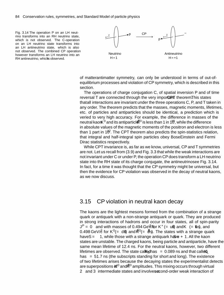
84 Conservation rules, symmetries, and Standard Model of particle physics
Fig. 3.14 The operation P on an LH neut-rino transforms into an RH neutrino state,which is not observed. The C-operationon an LH neutrino state transforms intoan LH antineutrino state, which is alsonot observed. The combined CP operationhowever transforms an LH neutrino into anRH antineutrino, which is observed.
ν�z �zp
p
CP
NeutrinoH = –1
AntineutrinoH = +1
ν
of matter–antimatter symmetry, can only be understood in terms of out-of-equilibrium processes and violation of CP symmetry, which is described in thissection.
The operations of charge conjugation C, of spatial inversion P and of timereversal T are connected through the very important CPT theorem. This statesthat all interactions are invariant under the three operations C, P, and T taken inany order. The theorem predicts that the masses, magnetic moments, lifetimes,etc. of particles and antiparticles should be identical, a prediction which isverified to very high accuracy. For example, the difference in masses of theneutral kaon K0 and its antiparticle K0 is less than 1 in 1019, while the differencein absolute values of the magnetic moments of the positron and electron is lessthan 1 part in 1012. The CPT theorem also predicts the spin-statistics relation,that integral and half-integral spin particles obey Bose–Einstein and Fermi–Dirac statistics respectively.
While CPT invariance is, as far as we know, universal, CP and T symmetriesare not. Let us recall from (3.9) and Fig. 3.3 that while the weak interactions arenot invariant under C or under P, the operation CP does transform a LH neutrinostate into the RH state of its charge conjugate, the antineutrino—see Fig. 3.14.In fact, for a time it was thought that the CP symmetry might be universal, butthen the evidence for CP violation was observed in the decay of neutral kaons,as we now discuss.
3.15 CP violation in neutral kaon decay
The kaons are the lightest mesons formed from the combination of a strangequark or antiquark with a non-strange antiquark or quark. They are producedin strong interactions of hadrons and occur in four states, all of spin-parityJ P = 0− and with masses of 0.494 GeV/c2 for K+(= us) and K−(= us), and0.498 GeV/c2 for K0(= ds) and K0(= d s). The states with a strange quarkhave S = −1, while those with a strange antiquark have S = +1. All the kaonstates are unstable. The charged kaons, being particle and antiparticle, have thesame mean lifetime of 12.4 ns. For the neutral kaons, however, two differentlifetimes are observed. The state called KS has τ = 0.089 ns and that called KL
has τ = 51.7 ns (the subscripts standing for ‘short’ and ‘long’). The existenceof two lifetimes arises because the decaying states the experimentalist detectsare superpositions of K0 and K0 amplitudes. This mixing occurs through virtual2π and 3π intermediate states and involves a second-order weak interaction of
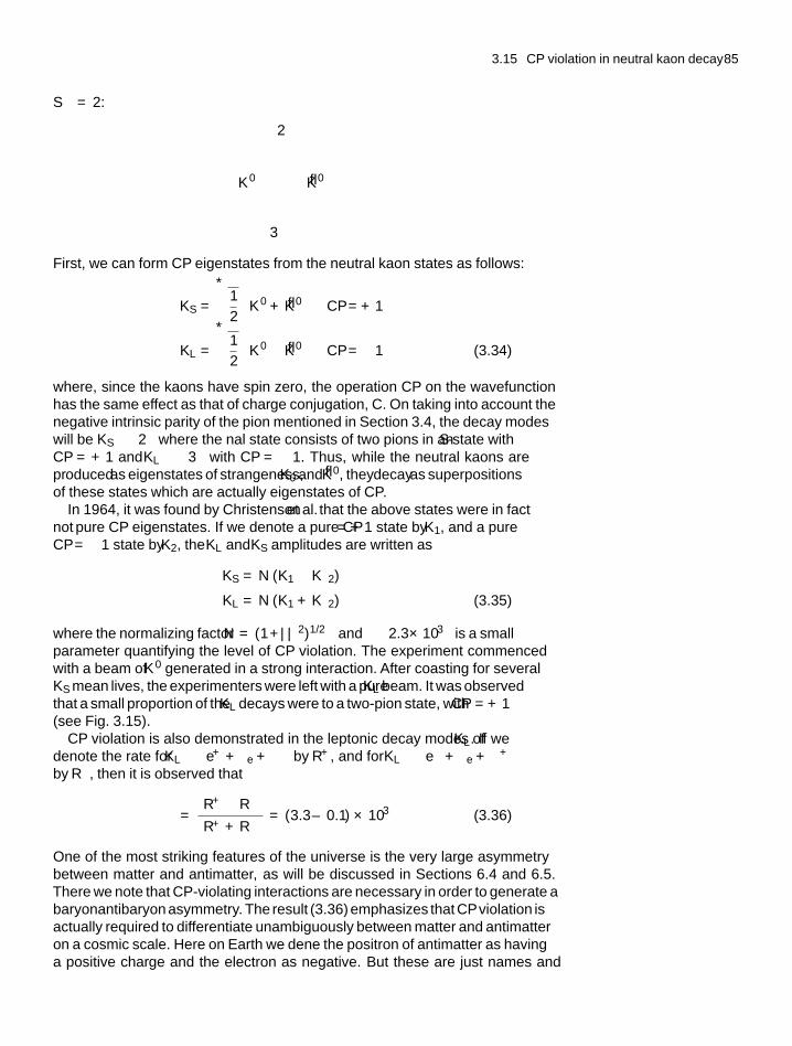
3.15 CP violation in neutral kaon decay 85
�S = 2:
2π
↗ ↘K0 K0
↘ ↙3π
First, we can form CP eigenstates from the neutral kaon states as follows:
KS =√
1
2
(K0 + K0
)CP = +1
KL =√
1
2
(K0 − K0
)CP = −1 (3.34)
where, since the kaons have spin zero, the operation CP on the wavefunctionhas the same effect as that of charge conjugation, C. On taking into account thenegative intrinsic parity of the pion mentioned in Section 3.4, the decay modeswill be KS → 2π where the final state consists of two pions in an S-state withCP = +1 and KL → 3π with CP = −1. Thus, while the neutral kaons areproduced as eigenstates of strangeness, K0 and K0, they decay as superpositionsof these states which are actually eigenstates of CP.
In 1964, it was found by Christenson et al. that the above states were in factnot pure CP eigenstates. If we denote a pure CP = +1 state by K1, and a pureCP = −1 state by K2, the KL and KS amplitudes are written as
KS = N (K1 − εK2)
KL = N (K1 + εK2) (3.35)
where the normalizing factor N = (1+|ε|2)−1/2 and ε ≈ 2.3×10⁻³ is a smallparameter quantifying the level of CP violation. The experiment commencedwith a beam of K0 generated in a strong interaction. After coasting for severalKS mean lives, the experimenters were left with a pure KL beam. It was observedthat a small proportion of the KL decays were to a two-pion state, with CP = +1(see Fig. 3.15).
CP violation is also demonstrated in the leptonic decay modes of KL. If wedenote the rate for KL → e+ + νe + π− by R+, and for KL → e− + νe + π+by R−, then it is observed that
� =(R+ − R−)(R+ + R−) = (3.3 ± 0.1) × 10−3 (3.36)
One of the most striking features of the universe is the very large asymmetrybetween matter and antimatter, as will be discussed in Sections 6.4 and 6.5.There we note that CP-violating interactions are necessary in order to generate abaryon–antibaryon asymmetry. The result (3.36) emphasizes that CPviolation isactually required to differentiate unambiguously between matter and antimatteron a cosmic scale. Here on Earth we define the positron of antimatter as havinga positive charge and the electron as negative. But these are just names and
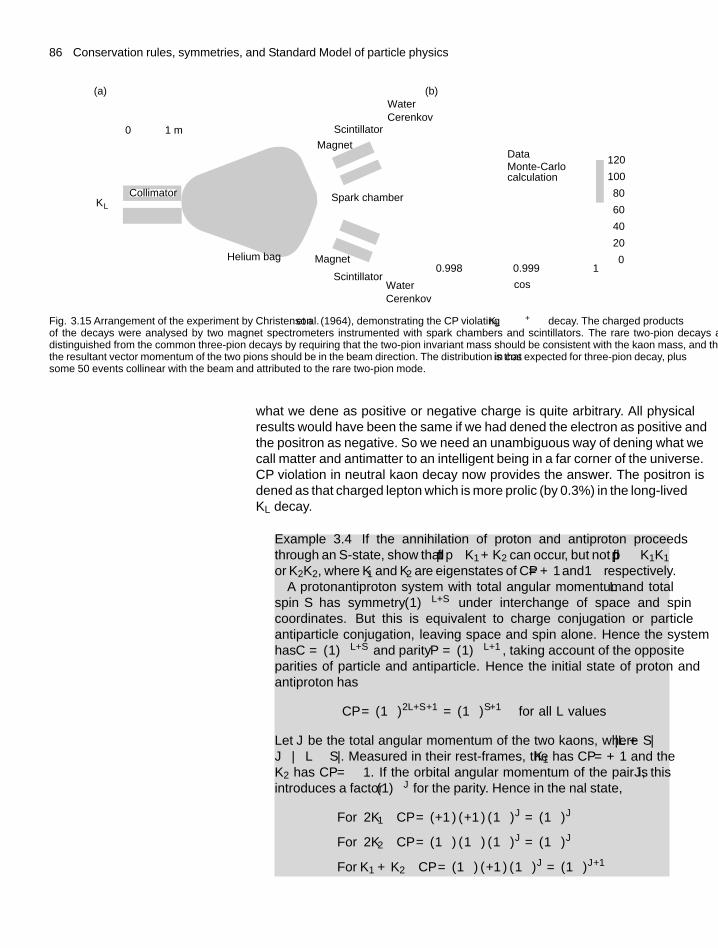
86 Conservation rules, symmetries, and Standard Model of particle physics
0 1 m
KL
Helium bag Magnet
Spark chamber
ScintillatorWaterCerenkov
Magnet
Scintillator
WaterCerenkov
DataMonte-Carlocalculation
0.998 0.999
cos �
1
20
0
40
60
120
100
80
(a) (b)
Collimator
Fig. 3.15 Arrangement of the experiment by Christenson et al. (1964), demonstrating the CP violating KL → π+π− decay. The charged productsof the decays were analysed by two magnet spectrometers instrumented with spark chambers and scintillators. The rare two-pion decays aredistinguished from the common three-pion decays by requiring that the two-pion invariant mass should be consistent with the kaon mass, and thatthe resultant vector momentum of the two pions should be in the beam direction. The distribution in cos θ is that expected for three-pion decay, plussome 50 events collinear with the beam and attributed to the rare two-pion mode.
what we define as positive or negative charge is quite arbitrary. All physicalresults would have been the same if we had defined the electron as positive andthe positron as negative. So we need an unambiguous way of defining what wecall matter and antimatter to an intelligent being in a far corner of the universe.CP violation in neutral kaon decay now provides the answer. The positron isdefined as that charged lepton which is more prolific (by 0.3%) in the long-livedKL decay.
Example 3.4 If the annihilation of proton and antiproton proceedsthrough an S-state, show that pp → K1 +K2 can occur, but not pp → K1K1
or K2K2, where K1 and K2 are eigenstates of CP = +1 and −1 respectively.A proton–antiproton system with total angular momentum L and total
spin S has symmetry (−1)L+S under interchange of space and spincoordinates. But this is equivalent to charge conjugation or particle–antiparticle conjugation, leaving space and spin alone. Hence the systemhas C = (−1)L+S and parity P = (−1)L+1, taking account of the oppositeparities of particle and antiparticle. Hence the initial state of proton andantiproton has
CP = (−1)2L+S+1 = (−1)S+1 for all L values
Let J be the total angular momentum of the two kaons, where |L + S| ≥J ≥ |L − S|. Measured in their rest-frames, the K1 has CP = +1 and theK2 has CP = −1. If the orbital angular momentum of the pair is J , thisintroduces a factor (−1)J for the parity. Hence in the final state,
For 2K1 CP = (+1) (+1) (−1)J = (−1)J
For 2K2 CP = (−1) (−1) (−1)J = (−1)J
For K1 + K2 CP = (−1) (+1) (−1)J = (−1)J+1
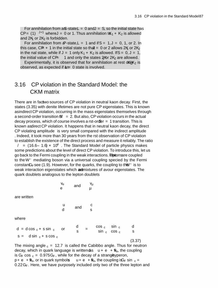
3.16 CP violation in the Standard Model 87
For annihilation from an S-state, L = 0 and J = S, so the initial state hasCP = (−1)J+1 where J = 0 or 1. Thus annihilation to K1 + K2 is allowedand 2K1 or 2K2 is forbidden.
For annihilation from a P-state, L = 1 and if S = 1, J = 0, 1, or 2. Inthis case, CP = +1 in the initial state so that J = 0 or 2 allows 2K1 or 2K2
in the final state, while if J = 1 only K1 + K2 is allowed. If S = 0, J = 1,the initial value of CP = −1 and only the states 2K1 or 2K2 are allowed.
Experimentally, it is observed that for annihilation at rest only K1K2 isobserved, as expected if an L = 0 state is involved.
3.16 CP violation in the Standard Model: theCKM matrix
There are in fact two sources of CP violation in neutral kaon decay. First, thestates (3.35) with definite lifetimes are not pure CP eigenstates. This is knownas indirect CP violation, occurring in the mass eigenstates themselves througha second-order transition of �S = 2. But also, CP violation occurs in the actualdecay process, which of course involves a first-order �S = 1 transition. This isknown as direct CP violation. It happens that in neutral kaon decay, the directCP violating amplitude ε′ is very small compared with the indirect amplitudeε. Indeed, it took more than 30 years from the first observation of CP violationto establish the existence of the direct process and measure it reliably. The ratioε′/ε = (16.6 ± 1.6) × 10−4. The Standard Model of particle physics makessome predictions about the level of direct CP violation. To introduce this, let usgo back to the Fermi coupling in the weak interactions. The leptons are coupledto the W ± mediating boson via a universal coupling specified by the Fermiconstant GF —see (1.9). However, for the quarks, the coupling to the W ± is toweak interaction eigenstates which are admixtures of flavour eigenstates. Thequark doublets analogous to the lepton doublets(
ve
e−)
and
(vμ
μ−)
are written (ud ′)
and
(cs′)
where
d ′ = d cos θc + s sin θc or
(d ′s′)
=(
cos θc sin θc
− sin θc cos θc
) (ds
)s′ = −d sin θc + s cos θc
(3.37)The mixing angle θc = 12.7◦ is called the Cabibbo angle. Thus for neutrondecay, which in quark language is written as d → u + e− + ve, the couplingis GF cos θc = 0.975 GF , while for the decay of a strange �-hyperon, � →p + e− + ve, or in quark symbols s → u + e− + ve, the coupling is GF sin θc =0.22 GF . Here, we have purposely included only two of the three lepton and
88 Conservation rules, symmetries, and Standard Model of particle physics
quark doublets in the above equation. When one includes all three families, thatis, the doublets (ντ , τ−) and (t, b), the transformation replacing (3.37) will bea 3 × 3 matrix called the CKM matrix after its proponents Cabibbo(1963) andKobayashi and Maskawa (1972).
This is written as ⎛⎝ d ′s′b′
⎞⎠ = VCKM
⎛⎝ dsb
⎞⎠where the absolute magnitudes of the (generally complex) elements of thematrix are
VCKM =∣∣∣∣∣∣
Vud Vus Vub
Vcd Vcs Vcb
Vtd Vts Vtb
∣∣∣∣∣∣ ≈∣∣∣∣∣∣
0.975 0.221 0.0040.221 0.975 0.0390.008 0.038 0.999
∣∣∣∣∣∣ (3.38)
The extreme off-diagonal elements Vtd and Vub are very small and not welldetermined.
The important point is that an N ×N matrix obviously contains N (N − 1)/2pairs, that is, Euler (mixing) angles, equal to 3 for N = 3 (compared withone for N = 2); and (N − 1) (N − 2)/2 arbitrary, non-trivial phases (i.e. onefor a 3 × 3 matrix and none for a 2 × 2). This phase δ in the CKM matrixenters the wavefunction as exp [i(ωt + δ)], which is not invariant under timereversal t → −t. So this is a possible T violating, or equivalently CP violating,amplitude in the Standard Model. The existence of this phase implies that someof the elements of the CKM matrix must be complex. Since on the hypothesisof universal Fermi coupling, the matrix V is unitary, the off-diagonal elementsof the product V ∗ V must be zero. So, for example, multiplying the top rowof the complex transpose matrix V * by the last column of V , we get for theright-hand top corner element of the product matrix
V ∗ud Vub + V ∗
cd Vcb + V ∗td Vtb = 0 (3.39)
and this can be plotted as a ‘unitarity triangle’ in the complex plane as shownin Fig. 3.16. The three angles α, β, and γ can be found by measurements onthe decays of neutral B-mesons, that is the quark–antiquark combinations bdand db, known as B0
d and B0d , and the combinations bs and bs, called B0
s andB0
s . For B-meson decays, the direct CP violation process is dominant over theindirect. Pair production of B−mesons in enormous quantity has been achievedat electron–positron colliders especially built for the purpose and called ‘B-factories’at Stanford, USA and KEK, Japan. Unlike the neutral kaons, the moremassive B-mesons have very many decay modes. The level of CP violation isobtained by measuring the difference in decay rates of B0 and B0 to the smallfraction of the decay modes that are common to both. For example, the decaysB0
d to ψKs, where the ψ is the ground state cc meson resonance, measure sin2β, while decays to π+π− measure sin 2α, and B0
s to ρKs measures sin 2γ . Theobject of these measurements is to determine whether the observed rates of CPviolation are consistent with the constraints of the Standard Model. Althoughnone has so far been observed, any departure from the unitarity relation (3.39)—non-closure of the triangle in Fig. 3.16—would be a signal of new physicsbeyond the Standard Model.
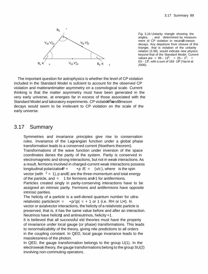
3.17 Summary 89
�
�
Bd → �+ �–
Bd → �KsBs → �Ks
Vtb V*td
Vcb V*cd
Vub V*ud
Fig. 3.16 ‘Unitarity triangle’ showing theangles α, β, and γ determined by measure-ment of CP violation in neutral B-mesondecays. Any departure from closure of thistriangle, that is violation of the unitarityrelation (3.39), would indicate new physicsbeyond that of the Standard Model. Currentvalues are α = 99 ± 110; β = 20 ± 10; γ =63 ± 130, with a sum of 182 ± 180 (Yao et al.2006).
The important question for astrophysics is whether the level of CP violationincluded in the Standard Model is sufficient to account for the observed CPviolation and matter–antimatter asymmetry on a cosmological scale. Currentthinking is that the matter asymmetry must have been generated in thevery early universe, at energies far in excess of those associated with theStandard Model and laboratory experiments. CP violation in K0 and B−mesondecays would seem to be irrelevant to CP violation on the scale of theearly universe.
3.17 Summary
• Symmetries and invariance principles give rise to conservationrules. Invariance of the Lagrangian function under a global phasetransformation leads to a conserved current (Noether’s theorem).
• Transformations of the wave function under inversion of the spacecoordinates defines the parity of the system. Parity is conserved inelectromagnetic and strong interactions, but not in weak interactions. Asa result, fermions involved in charged-current weak interactions possesslongitudinal polarization P = α
(σ · p)/E = α (v/c), where σ is the spin
vector (with σ 2 = 1), p and E are the three-momentum and total energyof the particle, and α = −1 for fermions and +1 for antifermions.
• Particles created singly in parity-conserving interactions have to beassigned an intrinsic parity. Fermions and antifermions have oppositeintrinsic parities.
• The helicity of a particle is a well-defined quantum number for ultra-relativistic particles; H = σ · p/|p| = +1 or −1 (i.e. RH or LH). Invector or axial–vector interactions, the helicity of a relativistic particle ispreserved, that is, it has the same value before and after an interaction.Neutrinos have helicity −1 and antineutrinos, helicity +1.
• It is believed that all successful field theories must have the propertyof invariance under local gauge (or phase) transformations. This leadsto renormalizability of the theory, giving finite predictions to all ordersin the coupling constant. In QED, local gauge invariance leads to themasslessness of the photon.
• In QED, the gauge transformation belongs to the group U(1). In theelectroweak theory, the gauge transformations belong to the group SU(2)involving non-commuting operators.
90 Conservation rules, symmetries, and Standard Model of particle physics
• Although the mediating bosons W and Z in the electroweak theory aremassive, the theory remains renormalizable as a result of the Higgsmechanism.
• In the simplest electroweak model, one physical scalar Higgs boson ispredicted. The present lower limit on the mass is about 100 GeV.
• The summation over Feynman graphs of higher orders can beapproximated by single boson exchange with an effective coupling which‘runs’ with the momentum transfer involved.
• Taking account of the virtual processes involved (radiative corrections),the electroweak theory predicts relations between the various parameters(particle masses, mixing angles, decay asymmetries, etc.) and these havebeen tested experimentally to high accuracy.
• All interactions are invariant under the C, P, and T operations taken inany order. This CPT invariance results in the same mass and lifetime forparticle and antiparticles and for the spin-statistics relation.
• CP invariance holds good in strong and electromagnetic interactions, butis violated in weak interactions. CP violation is allowed in the StandardModel of particle physics, with weak transformations between threefamilies of quarks and leptons. CP violation is required to account for thematter–antimatter asymmetry of the universe, although it is not clear thatthe violations observed in laboratory experiments on K0 and B-mesondecays are relevant to the cosmological problem.
Problems
More challenging problems are marked with an asterisk.
(3.1) Show that, if the pions are in a state of zero relativeorbital angular momentum (S-state), then π+π− isan eigenstate of CP = +1 and π+π−π0 is one ofCP = −1.
(3.2) Explain why the π+ and π− mesons are of equal mass,while the baryons �+ and �−, both of strangenessS = −1, have masses of 1189.4 MeV/c2 and 1197.4MeV/c2, respectively.
(3.3) The neutral non-strange mesons ρ0 (spin J = 1, mass770 MeV) and f 0 (J = 2, mass 1275 MeV) can bothdecay to π+π−. What are their C and P parities? Statewhich of the decays ρ0 → π0γ and f 0 → π0γ areallowed, and estimate the branching ratio.
(3.4) Show that the reaction π−+d → n+n+π0+Q (whereQ = 1.1 MeV) cannot proceed for pions at rest.
*(3.5) At energies of a few GeV, the cross-section for theelectromagnetic process e− + p → e− + hadrons ismuch larger than that for the weak process e− + p →νe + hadrons. However, at high energies and at high
enough values of the momentum transfer, the twoprocesses may have comparable cross-sections. Theseconditions would obtain, for example, at the HERAcollider at DESY, Hamburg, where 30 GeV electronscollide head-on with 820 GeV protons.
(a) Calculate the total collision energy at HERA inthe overall centre-of-momentum frame of theelectron and proton.
(b) If the primary collision is treated as between theelectron and a quasi-free u-quark carrying 25% ofthe proton momentum, what is the CMS energyof the electron–quark collision?
(c) At approximately what value of the four-momentum transfer squared (q2) betweenelectron and quark will the electromagnetic andweak cross-sections become equal? Refer toSection 1.9 for cross-section formulae.
(d) Write down any other process of electron–protonscattering which will be important at high q2.
*(3.6) On coming to rest in matter, a positron formsan ‘atomic’ S-state e+e− with an electron, called
Problems 91
positronium, which is observed to decay to two or threephotons, with two distinct lifetimes.
(a) What are the quantum numbers (total angularmomentum J , parity P, and charge conjugationparity C) of these states?
(b) The energy levels of the hydrogen atom aregiven by the formula En = −α2μc2/2n2, wheren is the principal quantum number and μ =mM /(m + M ) is the reduced mass of the proton,mass M , and the electron, mass m. Calculatethe n = 2 → n = 1 level spacing ineV in positronium (M = 938 MeV/c2, m =0.511 MeV/c2, α = 1/137).
(c) Try to estimate the lifetimes of the two decaymodes, based on the fact that electron andpositron wave functions have to overlap toannihilate, and that the Bohr radius in hydrogenis a = h/(μcα).
(3.7) Electron–positron annihilation at the appropriatelyhigh ‘resonant’ energy can result in the formationof the ϒ-meson (the upsilon meson) of mass 9460MeV/c2, which is a bound state of a ‘bottom’ quarkand antiquark: e+e− → bb → hadrons. Assuming thequark pair is in a state of orbital angular momentumL = 0, what are the quantum numbers J PC of theϒ-meson?
Energy levels due to radial excitations of thebb-system are observed above the ground state, thefirst such level being one of mass 10,023 MeV/c2.The corresponding 23S − 13S level separation inpositronium is 5.1 eV (see the previous question).Estimate the value of the strong coupling αs bindingthe quark and antiquark, assuming for simplicity a 1/r(Coulombic) interquark potential (i.e. the first termin (1.7)).
*(3.8) Write down how the following quantities willtransform under the P (space inversion) and T
(time reversal) operations:
Position coordinate rMomentum vector pSpin/angular momentum vector σ = r × pElectric field E = −∇VMagnetic field B = i × rElectric dipole moment σ · EMagnetic dipole moment σ · BLongitudinal polarization σ · p
Show that an electric dipole moment for theneutron would violate T -invariance. Try to estimatean upper limit to such a dipole moment, assuming theappropriate level of CP invariance is that observed inneutral kaon decay.
Estimate the expected level of asymmetry in thescattering of polarized protons by polarized protons(the polarization being longitudinal).
(3.9) All of the following decays are allowed by energyconservation. Which of them is allowed by otherconservation laws? (Note: The ρ-meson has J P = 1−.The π and η-mesons have J P = 0−, and their principaldecay modes are to two photons):
ρ0 → π+ + π− ρ0 → η + γ
ρ0 → π0 + π0 ρ0 → π0 + η
π0 → γ + e+ + e− η → e+ + e−
*(3.10) In a deep inelastic neutrino–nucleon collision, thequark–parton model (Section 3.12.1) predicts apointlike cross-section proportional to energy, as in(1.27b). Above a few GeV energy, the observedneutrino–nucleon cross-section has the value σ/E =6.7 × 10−39 cm2, where E is the neutrino energyin GeV. Calculate the average fractional momentum ofthe nucleon which is carried by the parton in such acollision.
4 Extensions of theStandard Model
The Standard Model described in Chapter 3, which has given a magnificentlyaccurate account of a huge range of data from accelerator experiments since itsinception, does, however, have limitations. As examples, it assumes neutrinosare massless, in conflict with recent experimental results, and has theoreticaldifficulties with topics as diverse as the so-called hierarchy problem, or ofaccounting for the baryon asymmetry of the universe. As will be indicatedin later chapters, it is indeed on the scale of the universe that it fails totake into account completely new forms of matter and energy, which haveonly really become apparent since the Standard Model was first introducedin the mid-1970s. Finally of course, it does not include gravity. Includinggravity with the other fundamental interactions is still an unsolved problem. Ofcourse, we do not know what better theory will eventually replace the StandardModel, although whatever that is, the Standard Model will surely be a partof it. In this chapter, we just outline some new directions in physics goingbeyond it.
4.1 Neutrinoless double beta decay
As was pointed out in Chapter 1, the question as to the nature of neutrinos—whether they are Dirac or Majorana particles—is still open. In the StandardModel, neutrinos are assumed to be massless—an assumption in accordwith all the data available when the Standard Model first appeared. But, asdescribed below, evidence from neutrino flavour oscillations, appearing after1990 showed the neutrino masses to be finite, although very small. Thefact that the masses of the light neutrinos, of order 0.1 eV/c2, are someten orders of magnitude less than the typical masses of the known Diracparticles, such as quarks and charged leptons, suggests that they might indeedbe Majorana particles, the smallness of the mass arising from the so-calledsee-saw mechanism described below.
If neutrinos are indeed Majorana particles, lepton number L is violated, sinceneutrinos (L = 1 in the Dirac picture) are then identical with antineutrinos(L = −1). However, the proof of this can be easily found by only one type ofobservation, namely that of neutrinoless double beta decay.
We know that, in ordinary nuclear beta decay, the emitted electron isaccompanied by an (anti)neutrino, for example, in neutron decay:
n −→ p + e− + ve (4.1)
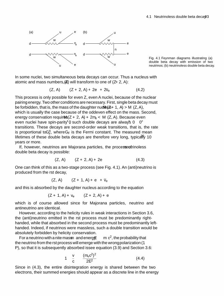
4.1 Neutrinoless double beta decay 93
d d
dd
u
w– w–
w–w–
u
u
u
n
e–
e–
e–
e–ne–
ne–
(a) (b)
Fig. 4.1 Feynman diagrams illustrating (a)double beta decay with emission of twoneutrinos; (b) neutrinoless double beta decay.
In some nuclei, two simultaneous beta decays can occur. Thus a nucleus withatomic and mass numbers (Z , A) will transform to one of (Z + 2, A):
(Z , A) −→ (Z + 2, A) + 2e− + 2ve (4.2)
This process is only possible for even Z, even A nuclei, because of the nuclearpairing energy. Two other conditions are necessary. First, single beta decay mustbe forbidden, that is, the mass of the daughter nucleus M (Z+1, A) > M (Z, A),which is usually the case because of the odd–even effect on the mass. Second,energy conservation requires M (Z + 2, A) + 2me < M (Z, A). Because even–even nuclei have spin-parity 0+, such double decays are always 0+ → 0+transitions. These decays are second-order weak transitions, that is, the rateis proportional to G4
F, where GF is the Fermi constant. The measured meanlifetimes of these double beta decays are therefore very long, typically 1020
years or more.If, however, neutrinos are Majorana particles, the process of neutrinoless
double beta decay is possible:
(Z , A) −→ (Z + 2, A) + 2e− (4.3)
One can think of this as a two-stage process (see Fig. 4.1). An (anti)neutrino isproduced from the first decay,
(Z , A) −→ (Z + 1, A) + e− + ve
and this is absorbed by the daughter nucleus according to the equation
(Z + 1, A) + ve −→ (Z + 2, A) + e−
which is of course allowed since for Majorana particles, neutrino andantineutrino are identical.
However, according to the helicity rules in weak interactions in Section 3.6,the (anti)neutrino emitted in the first process must be predominantly right-handed, while that absorbed in the second process must be predominantly left-handed. Indeed, if neutrinos were massless, such a double transition would beabsolutely forbidden by helicity conservation.
For a neutrino with a finite mass mν and energy E � mνc2, the probability thatthe neutrino from the first process will emerge with the ‘wrong’polarization (1−P), so that it is subsequently absorbed is—see equation (3.9) and Section 3.6:(
1 − v
c
)∼ (mvc2)2
2E2(4.4)
Since in (4.3), the entire disintegration energy is shared between the twoelectrons, their summed energies should appear as a discrete line in the energy
94 Extensions of the Standard Model
spectrum. (However, since it is a very rare process—if it occurs at all—theobservation of neutrinoless double beta decay is likely to involve massivedetectors and far from ideal resolution.) So far, neutrinoless double beta decayhas not been observed, and limits on the lifetime exceed 1025 years. Withoutgoing into the complex details of the calculation of the nuclear matrix elementsneeded to compute the transition rate, and its considerable uncertainties, onecan see from (4.4) that this lifetime limit must correspond to an upper limit onthe neutrino mass, which is currently given in the range
Absence of neutrinoless double beta decay −→ mvc2 < 0.3 − 2 eV (4.5)
applying of course to the electron neutrino νe; see Klapdor-Kleingrothaus et al.(2001) and Fiorini (2005). This limit is still, however, considerably larger thanthe mass differences (<0.1 eV)—and by inference, the masses themselves—from observation of neutrino oscillations discussed below, and more fullydescribed in Chapter 9. The observation of neutrinoless double beta decaywould be extremely important, not simply because, if observed, it would provebeyond doubt our suspicion that neutrinos really are Majorana particles but alsobecause from the observations one might hope to measure certain CP violatingphases. Such phases could play a vital role in the decay of massive Majorananeutrinos, which could generate a lepton and baryon asymmetry in the earlyuniverse, as discussed in Section 6.5.
4.2 Neutrino masses and flavour oscillations
In the original Standard Model formulated in the 1970s, neutrinos are assumedto be massless and exist in only one (left-handed) helicity state. However,the assumed masslessness of neutrinos was questioned many years ago, inconnection with the possibility of flavour oscillations. (The first proposal,by Pontecorvo, related to neutrino–antineutrino oscillations–in analogy with
K0 − K0
mixing – for which there is no evidence and which is not consideredfurther.) Later Maki, Nakagaya, and Sakata (1962), Pontecorvo (1967), andGribov and Pontecorvo (1969) proposed that, while neutrinos are createdor destroyed as flavour eigenstates, they propagate through space as masseigenstates. The situation is analogous to that in the quark sector, whereweak interaction eigenstates are superpositions of strong flavour eigenstates. Aparticular neutrino flavour eigenstate, denoted by the amplitude νe, νμ, or ντ
is therefore expressed, as regards its time evolution, as a linear superpositionν1, ν2, and ν3 of mass eigenstates, which propagate through space with slightlydifferent frequencies due to their different masses, and between which differentphases develop with distance traversed, corresponding to a change or oscillationin the neutrino flavour. Thus a neutrino, created with a unique flavour, aftertraversing some distance in space will become a superposition of differentflavours, as evidenced by any subsequent interaction with matter.
The 3×3 matrix connecting neutrino flavour and mass eigenstates isanalogous to the CKM matrix (3.38) connecting quark flavour (stronginteraction) eigenstates with the weak decay eigenstates. Again, the matrixinvolves the mixing angles between the mass eigenstates, as well as a possibleCP violating phase angle. For a matrix of dimension ‘n’ the number of possible
4.2 Neutrino masses and flavour oscillations 95
(Euler) mixing angles is clearly n (n − 1)/2, which is 3 for n = 3, and thepossible number of non-trivial CP violating phases is (n − 1)(n − 2)/2 = 1.However, to begin with and to simplify the treatment we shall consider the caseof just two flavours, with just a single mixing angle θ and no CP violation. Infact, as shown below, it turns out that, since one of the three mixing angles isvery small—but from the experimentalist’s point of view, hopefully not zero—and the other two are large, the actual effects observed to date can be accountedfor, at least to present experimental accuracies, in terms of twofold mixingonly. Using neutrino symbols to denote the wave amplitudes of the particlesinvolved, let us, for example, consider the mixing of νμ and ντ in terms of ν2
and ν3 (the practical situation for atmospheric neutrinos):(vμ
vτ
)=(
cos θ sin θ
− sin θ cos θ
)(v2
v3
)(4.6)
where θ denotes some arbitrary mixing angle. The wave amplitudes
vμ = v2 cos θ + v3 sin θ
vτ = −v2 sin θ + v3 cos θ (4.7)
are orthonormal states. If E denotes the neutrino energy, the amplitudes of themass eigenstates as a function of time will be
v2(t) = v2(0) exp(−iE2t)
v3(t) = v3(0) exp(−iE3t) (4.8)
where we have used units h = c = 1, so the angular frequency ω = E. The masseigenstates will have a fixed momentum p, so that if the masses are mi Ei
(where i = 2, 3),
Ei = p + m2i
2p(4.9)
Suppose that we start off at t = 0 with muon-type neutrinos, that is, νμ(0) = 1and ντ(0) = 0. Inverting (4.6) we have
v2(0) = vμ(0) cos θ
v3(0) = vμ(0) sin θ (4.10)
and
vμ(t) = v2(t) cos θ + v3(t) sin θ
From (4.8) and (4.10) the amplitude of the muon–neutrinos becomes
Aμ(t) = vμ(t)
vμ(0)= cos2 θ exp (−iE2t) + sin2 θ exp (−iE3t)
so that the intensity is
Iμ(t)
Iμ(0)= AA∗ = 1 − sin2 2θ sin2
[(E3 − E2) t
2
]We use (4.9) and write the difference of the squares of the masses as �m2 =m2
3 −m22, where here and in what follows we assume m3 > m2. The probability
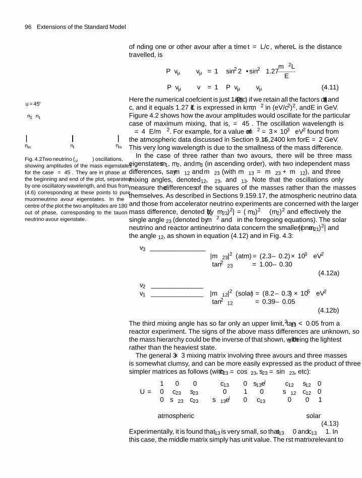
96 Extensions of the Standard Model
of finding one or other flavour after a time t = L/c, where L is the distancetravelled, is
P(vμ −→ vμ
) = 1 − sin2 2θ · sin2(
1.27�m2L
E
)P(vμ −→ vτ
) = 1 − P(vμ −→ vμ
)(4.11)
Here the numerical coefficient is just 1/(4hc) if we retain all the factors of h andc, and it equals 1.27 if L is expressed in km, �m2 in (eV/c2)2, and E in GeV.Figure 4.2 shows how the flavour amplitudes would oscillate for the particularcase of maximum mixing, that is, θ = 45◦. The oscillation wavelength isλ = 4πE/�m2. For example, for a value of �m2 = 3 × 10⁻³ eV2 found fromthe atmospheric data discussed in Section 9.15, λ = 2400 km for E = 2 GeV.This very long wavelength is due to the smallness of the mass difference.
n2 n1
nt nmnm
u = 45°
Fig. 4.2 Two neutrino (νμ → ντ) oscillations,showing amplitudes of the mass eigenstatesfor the case θ = 45◦. They are in phase atthe beginning and end of the plot, separatedby one oscillatory wavelength, and thus from(4.6) corresponding at these points to puremuon–neutrino flavour eigenstates. In thecentre of the plot the two amplitudes are 180◦out of phase, corresponding to the tauon–neutrino flavour eigenstate.
In the case of three rather than two flavours, there will be three masseigenstates m1, m2, and m3 (in ascending order), with two independent massdifferences, say �m12 and �m23 (with �m13 = �m23 + �m12), and threemixing angles, denoted θ12, θ23, and θ13. Note that the oscillations onlymeasure the differences of the squares of the masses rather than the massesthemselves. As described in Sections 9.15–9.17, the atmospheric neutrino dataand those from accelerator neutrino experiments are concerned with the largermass difference, denoted by |(�m23)
2| = (m3)2 − (m2)
2 and effectively thesingle angle θ23 (denoted by �m2 and θ in the foregoing equations). The solarneutrino and reactor antineutrino data concern the smaller one, |(�m21)
2| andthe angle θ12, as shown in equation (4.12) and in Fig. 4.3:
v3 _______________← |�m23|2 (atm) = (2.3 ± 0.2) × 10−3 eV2
tan2 θ23 = 1.00 ± 0.30(4.12a)
v2 ______________v1 ______________ ← |�m12|2 (solar) = (8.2 ± 0.3) × 10−5 eV2
tan2 θ12 = 0.39 ± 0.05(4.12b)
The third mixing angle has so far only an upper limit, tan2θ13 < 0.05 from areactor experiment. The signs of the above mass differences are unknown, sothe mass hierarchy could be the inverse of that shown, with ν3 being the lightestrather than the heaviest state.
The general 3 × 3 mixing matrix involving three flavours and three massesis somewhat clumsy, and can be more easily expressed as the product of threesimpler matrices as follows (with c23 = cos θ23, s23 = sin θ23, etc):
U =∣∣∣∣∣∣
1 0 00 c23 s23
0 −s23 c23
∣∣∣∣∣∣∣∣∣∣∣∣
c13 0 s13eiδ
0 1 0−s13e−iδ 0 c13
∣∣∣∣∣∣∣∣∣∣∣∣
c12 s12 0−s12 c12 0
0 0 1
∣∣∣∣∣∣↑ ↑
atmospheric solar(4.13)
Experimentally, it is found that θ13 is very small, so that s13 ∼ 0 and c13 ∼ 1. Inthis case, the middle matrix simply has unit value. The first matrix—relevant to
4.3 Grand unified theories: proton decay 97
Atmospheric+
Accelerator
Solar + Reactor
+
+
10–2
10–3
�m
2(e
V2 )
tan2 u
10–4
10–1 1 10
Fig. 4.3 Plots of �m2, the square of themass difference, against tan2 θ where θ isthe mixing angle. At top, the combinedatmospheric and long baseline acceleratordata; and at bottom the solar (νe) andreactor (ve) combined data (assuming CPTinvariance). The boundaries of the shadedareas correspond to 90% confidence limits.
atmospheric neutrino oscillations—depends only on θ23, while the third matrix,relevant to solar neutrinos, depends only on θ12. The solar and atmosphericneutrinos are therefore effectively decoupled, since they are only connectedvia θ13. The CP violating phase δ is seen to enter only multiplied by the smallquantity sin θ13, so that it will be very hard to detect. The experimental situationleading to the foregoing results is described in Chapter 9.
4.3 Grand unified theories: proton decay
The success of the electroweak theory, unifying the electromagnetic and weakinteractions, in describing an enormous range of experimental data, opened thepossibility that unification of the fundamental interactions might be taken onestage further, by incorporating the strong interactions with the electroweak, inwhat are called grand unified theories—GUTs for short. The basic idea is thatthe SU(2) × U(1) electroweak symmetry (a broken symmetry at low energies)plus the (exact) SU(3) colour symmetry of the strong interactions might beencompassed by a more global symmetry, manifested at some high unificationenergy, where the component symmetries would become exact. Since theeffective couplings for the different interactions ‘run’ in different ways, thepossibility arose that they might extrapolate to a universal value, the grandunified coupling αu. This possible extension of the Standard Model was firstdiscussed in the early 1970s, shortly after the success of the electroweak theory.
The first and simplest GUT model was the SU(5) model of Georgi andGlashow (1974). This incorporated the fermions, both leptons and quarks, intomultiplets, inside which, with a common coupling, leptons and quarks couldtransform into one another via the exchange of massive ‘leptoquark’ bosons
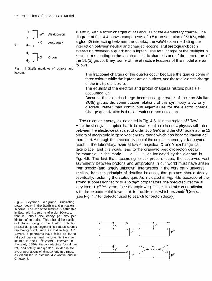
98 Extensions of the Standard Model
neW6 Weak boson
Leptoquark“5” =
Gluon
X
G
e–
dR–
dB–
dG–
Fig. 4.4 SU(5) multiplet of quarks andleptons.
X and Y , with electric charges of 4/3 and 1/3 of the elementary charge. Thediagram of Fig. 4.4 shows components of a ‘5’ representation of SU(5), witha gluon G interacting between the quarks, the weak W boson mediating theinteraction between neutral and charged leptons, and the X ‘leptoquark’ bosoninteracting between a quark and a lepton. The total charge of the multiplet iszero, corresponding to the fact that electric charge is one of the generators ofthe SU(5) group. Briefly, some of the attractive features of this model are asfollows:
• The fractional charges of the quarks occur because the quarks come inthree colours while the leptons are colourless, and the total electric chargeof the multiplets is zero.
• The equality of the electron and proton charges—a historic puzzle—isaccounted for.
• Because the electric charge becomes a generator of the non-AbelianSU(5) group, the commutation relations of this symmetry allow onlydiscrete, rather than continuous eigenvalues for the electric charge.Charge quantization is thus a result of grand unification.
The unification energy, as indicated in Fig. 4.6, is in the region of 1014 GeV.Here the strong assumption has to be made that no other ‘new’physics will enterbetween the electroweak scale, of order 100 GeV, and the GUT scale some 12orders of magnitude larger—a vast energy range which has become known asthe desert. Although the predicted value of the unification energy is far beyondreach in the laboratory, even at low energies virtual X and Y exchange cantake place, and this would lead to the dramatic prediction of proton decay,for example, in the mode p → e+ + π0, as indicated by the diagram inFig. 4.5. The fact that, according to our present ideas, the observed vastasymmetry between protons and antiprotons in our world must have arisenfrom specific (and largely unknown) interactions in the very early universeimplies, from the principle of detailed balance, that protons should decayeventually, restoring the status quo. As indicated in Fig. 4.5, because of thestrong suppression factor due to the X , Y propagators, the predicted lifetime isvery long, 10(30±0.5) years (see Example 4.1). This is in definite contradictionwith the experimental lower limit to the lifetime, which exceeds 1033 years.(see Fig. 4.7 for detector used to search for proton decay).
Fig. 4.5 Feynman diagrams illustratingproton decay in the SU(5) grand unificationscheme. The expected lifetime is estimatedin Example 4.1 and is of order 1030 years,that is, about one decay per day perkiloton of material. This should be easilydetectable using a multikiloton detectorplaced deep underground to reduce cosmicray background, such as that in Fig. 4.7.Several experiments have failed so far tofind such decays, and the lower limit on thelifetime is about 1033 years. However, inthe early 1990s these detectors found thefirst, and totally unexpected, evidence forflavour oscillations of atmospheric neutrinos,as discussed in Section 4.2 above and inChapter 9.
u
u
u
u
u
u
u
u
d
d
d
d
d
X Y
YY
e+
e+
e+
e+
p0
p0
p0
p0u
uu
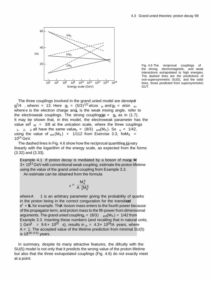
4.3 Grand unified theories: proton decay 99
1/a
1/a1
1/a2
1/a3
Energy scale (GeV)
60
40
20
102 104 106 108 1010 1012 1014 1016 1018
Fig. 4.6 The reciprocal couplings ofthe strong, electromagnetic, and weakinteractions extrapolated to high energies.The dashed lines are the predictions ofnon-supersymmetric SU(5), and the solidlines, those predicted from supersymmetricGUT.
The three couplings involved in the grand unified model are denoted αi =g2
i /4π, where i = 1−3. Here g1 = (5/3)1/2 e/cos θw and g2 = e/sin θw,where e is the electron charge and θw is the weak mixing angle, refer tothe electroweak couplings. The strong coupling is g3 = gs as in (1.7).It may be shown that, in this model, the electroweak parameter has thevalue sin2 θW = 3/8 at the unification scale, where the three couplingsα1, α2, α3 all have the same value αu = (8/3) αem(MX ). So αu = 1/42,using the value of αem (MX ) = 1/112 from Exercise 3.3, for MX =1014 GeV.
The dashed lines in Fig. 4.6 show how the reciprocal quantities 1/α1,2,3 varylinearly with the logarithm of the energy scale, as expected from the forms(3.32) and (3.33).
Example 4.1 If proton decay is mediated by a boson of mass MX =3×10¹⁴ GeV with conventional weak coupling, estimate the proton lifetimeusing the value of the grand unified coupling from Example 3.3.
An estimate can be obtained from the formula
τp = M 4X
Aα2uM 5
p
where A ∼ 1 is an arbitrary parameter giving the probability of quarksin the proton being in the correct configuration for the transition ud →e+ + u, for example. The X -boson mass enters to the fourth power becauseof the propagator term, and proton mass to the fifth power from dimensionalarguments. The grand unified coupling αu = (8/3) αem(MX ) = 1/42 fromExample 3.3. Inserting these numbers (and recalling that in natural units,1 GeV−1 = 9.6 × 10⁻²⁵ s), results in τp = 4.3 × 1029/A years, whereA < 1. The accepted value of the lifetime prediction from minimal SU(5)is 10(30±0.5) years.
In summary, despite its many attractive features, the difficulty with theSU(5) model is not only that it predicts the wrong value of the proton lifetimebut also that the three extrapolated couplings (Fig. 4.6) do not exactly meetat a point.
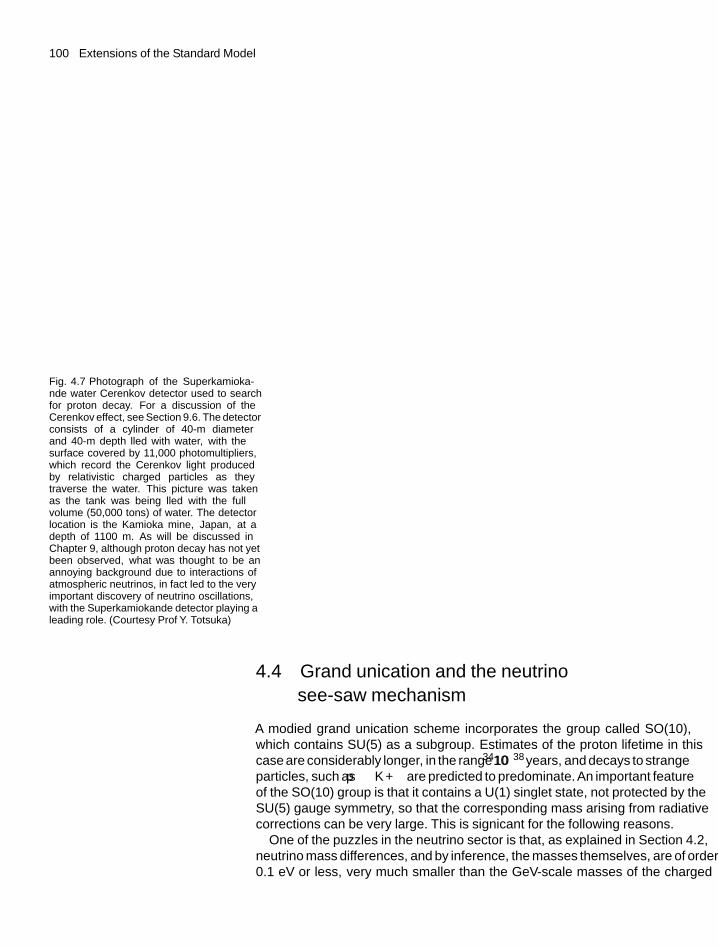
100 Extensions of the Standard Model
Fig. 4.7 Photograph of the Superkamioka-nde water Cerenkov detector used to searchfor proton decay. For a discussion of theCerenkov effect, see Section 9.6. The detectorconsists of a cylinder of 40-m diameterand 40-m depth filled with water, with thesurface covered by 11,000 photomultipliers,which record the Cerenkov light producedby relativistic charged particles as theytraverse the water. This picture was takenas the tank was being filled with the fullvolume (50,000 tons) of water. The detectorlocation is the Kamioka mine, Japan, at adepth of 1100 m. As will be discussed inChapter 9, although proton decay has not yetbeen observed, what was thought to be anannoying background due to interactions ofatmospheric neutrinos, in fact led to the veryimportant discovery of neutrino oscillations,with the Superkamiokande detector playing aleading role. (Courtesy Prof Y. Totsuka)
4.4 Grand unification and the neutrinosee-saw mechanism
A modified grand unification scheme incorporates the group called SO(10),which contains SU(5) as a subgroup. Estimates of the proton lifetime in thiscase are considerably longer, in the range 1034–1038 years, and decays to strangeparticles, such as p → K+π are predicted to predominate. An important featureof the SO(10) group is that it contains a U(1) singlet state, not protected by theSU(5) gauge symmetry, so that the corresponding mass arising from radiativecorrections can be very large. This is significant for the following reasons.
One of the puzzles in the neutrino sector is that, as explained in Section 4.2,neutrino mass differences, and by inference, the masses themselves, are of order0.1 eV or less, very much smaller than the GeV-scale masses of the charged
4.4 Grand unification and the neutrino see-saw mechanism 101
leptons and quarks. As explained in Chapter 1, charged leptons are describedby the Dirac equation, and both left-handed and right-handed helicity statesψL and ψR occur. In fact, the mass term in the Dirac equation is of the formψLψR (and the mass itself is obtained by multiplying by the Higgs coupling).Neutrinos, if they are pure Dirac particles (so that neutrinos and antineutrinosare distinct particle and antiparticle), would therefore have exactly zero massif they only existed in the left-handed state ψL, as is supposed in the StandardModel. The other possibility is that they are Majorana particles, where particleand antiparticle are identical. In general, we could suppose that lepton massesresult from a mixture of both Dirac and Majorana mass terms. Because, forcharged leptons, particle and antiparticle are clearly distinct, they must be pureDirac particles, while neutrinos and antineutrinos can be a mixture of the twotypes. Suppose we denote the Majorana masses as mL and mR for the left-and right-handed states. The neutrino mass matrix operating on the neutrinowavefunctions can be a combination of Majorana mR,L and Dirac mD massterms, written in the form ∣∣∣∣ mL mD
mD mR
∣∣∣∣ (4.14)
By setting this matrix into diagonal form, the eigenvalues are readily foundto be
m1,2 = 1
2
[(mR + mL) ±
√(mR − mL)2 + 4m2
D
](4.15)
Suppose now that mL is very small (and we shall set it to zero), and that mR = Mis very large compared with the Dirac scale, and of the order of the GUT massscale. Then the physical neutrino masses become
m1 ≈ (mD)2
Mm2 ≈ M (4.16)
One ends up therefore with a left-handed Majorana neutrino of very small mass,forced down because of the large mass M of the right-handed neutrino—what istermed the ‘see-saw’mechanism. Of course, both the light- and heavy neutrinoswill exist as both left- and right-handed states, and presumably will be replicatedin three flavour states. If we take 10 GeV as a typical Dirac mass, a value ofM ∼ 1012 Gev yields m1 ∼ 0.1 eV, which is in the range of light neutrinomasses actually observed. This so-called see-saw mechanism therefore relieson the existence of massive Majorana neutrinos to suppress the light neutrinomass well below the Dirac mass scale.
If this view is correct, the smallness of the observed neutrino masses impliesnew interactions and new physics at a very-high-energy scale, perhaps that ofgrand unification discussed above. Furthermore, as is discussed in Chapter 6,it also appears that the decay of such massive neutrinos could result in a leptonasymmetry, converted to a baryon asymmetry by so-called instanton effectsat the electroweak scale, of roughly the correct magnitude to account for theobserved matter–antimatter asymmetry of the universe. So some vital featuresof our universe seem to hang on the knotty problem of the nature and masses ofneutrinos. These predictions, arising from the results of neutrino experimentsduring the 1990s, of course have very deep and important implications forcosmology.
102 Extensions of the Standard Model
4.5 Hierarchies and supersymmetry
Another unification scheme includes the idea of supersymmetry, alreadymentioned in Section 1.3, wherein every fermion has a boson partner;conversely, for each fundamental boson there is a supersymmetric fermionpartner. Supersymmetry was postulated as a way of avoiding the so-calledhierarchy problem. In Chapter 3 we noted that the very successful calculationof radiative corrections to the Standard Model involved loops containing virtualfermions and bosons. However, if there exist very massive particles associatedwith grand unified symmetry schemes, they will be present as virtual statesin such loops and lead to divergences in calculating the Standard Modelparameters, unless one can arrange cancellation terms. Supersymmetry doesjust that, since it turns out that the amplitudes for fermion and boson loopshave opposite signs (technically connected with the fact that the creation andannihilation operators for bosons and fermions obey commutation and anti-commutation relations, respectively). Thus the one-loop radiative correction tothe Higgs mass is of the form �m2
H ∼ (α/π)(m2
F − m2B
)and, provided the
mass scale of the superpartners is less than about 1 TeV, the strong (quadratic)divergences are avoided (although much smaller, logarithmic divergencesremain). A bonus of this scheme is that above the SUSY (= supersymmetry)scale, the evolution of the three running couplings is modified and they do meetmore nearly at a point, as shown in Fig. 4.6, with a higher unification energyof around 1016 GeV. Because of the larger MX , the expected proton lifetime islonger, of order 1035 years, which is compatible with the experimental limit.As stated previously, in this modified unification scheme, the preferred protondecay modes are into heavier particles, for example, p → K+ + νμ.
At the present time, there is no direct experimental support for supersymmetryor for grand unification. Lower limits on the masses of SUSY particles fromaccelerators are ∼100 GeV. This is of course larger than the masses of mostof the known fundamental fermions and bosons. Clearly, supersymmetry is abroken symmetry, and it could be that all the superpartners have masses in therange 100–1000 GeV. A list of some SUSY particles is given in Table 4.1. Aword should be added about notation. The boson superpartners of the fermionsare denoted by adding an ‘s’prefix; thus squark, slepton, and so on. The fermionsuperpartners of the bosons are denoted by adding ‘ino’ after the name; forexample, photino, zino, gluino, and so on.
Most supersymmetric models postulate an R-symmetry, that is, the SUSYparticles are produced in pairs with conserved quantum numbers R = ±1, inmuch the same way that strange particles are pair-produced with S = ±1 inconventional strong interactions. Thus a quark and antiquark with sufficientenergy could annihilate to a squark–antisquark pair. A massive SUSY particlewould decay, in an R-conserving cascade process, to lighter SUSY particles,and eventually to the lightest superparticle, which, in the limit of exact R-conservation, would be completely stable. If this were a photino, for example,its production from squark decay, Q → Q+γ would be manifest by acoplanarityof the decay and momentum imbalance from the missing photino.
The so-called minimal supersymmetric standard model (MSSM) of courseencompasses a host of new particles, including a richer Higgs sector withfive physical Higgs bosons. The SUSY partners of the four electroweak gaugebosons consist of four neutral fermions, referred to as neutralinos. As will be
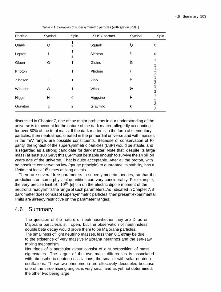
4.6 Summary 103
Table 4.1 Examples of supersymmetric particles (with spin in units h/2π)
Particle Symbol Spin SUSY partner Symbol Spin
Quark Q1
2Squark Q 0
Lepton l1
2Slepton l 0
Gluon G 1 Gluino G1
2
Photon γ 1 Photino γ1
2
Z boson Z 1 Zino Z1
2
W boson W 1 Wino W1
2
Higgs H 0 Higgsino H1
2
Graviton g 2 Gravitino g3
2
discussed in Chapter 7, one of the major problems in our understanding of theuniverse is to account for the nature of the ‘dark matter’, allegedly accountingfor over 80% of the total mass. If the dark matter is in the form of elementaryparticles, then neutralinos, created in the primordial universe and with massesin the TeV range, are possible constituents. Because of conservation of R-parity, the lightest of the supersymmetric particles (LSP) would be stable, andis regarded as a strong candidate for dark matter. Note that, despite its largemass (at least 100 GeV) this LSP must be stable enough to survive the 14 billionyears age of the universe. That is quite acceptable. After all the proton, withno absolute conservation law (gauge principle) to guarantee its stability, has alifetime at least 1023 times as long as this.
There are several free parameters in supersymmetric theories, so that thepredictions on some physical quantities can vary considerably. For example,the very precise limit of < 10−25|e| cm on the electric dipole moment of theneutron already limits the range of such parameters. As indicated in Chapter 7, ifdark matter does consist of supersymmetric particles, then present experimentallimits are already restrictive on the parameter ranges.
4.6 Summary
• The question of the nature of neutrinos—whether they are Dirac orMajorana particles—is still open, but the observation of neutrinolessdouble beta decay would prove them to be Majorana particles.
• The smallness of light neutrino masses, less than 0.1 eV/c2, may be dueto the existence of very massive Majorana neutrinos and the ‘see-saw’mixing mechanism.
• Neutrinos of a particular flavour consist of a superposition of masseigenstates. The larger of the two mass differences is associatedwith atmospheric neutrino oscillations, the smaller with solar neutrinooscillations. These two phenomena are effectively decoupled becauseone of the three mixing angles is very small and as yet not determined,the other two being large.
104 Extensions of the Standard Model
• The success of the electroweak model led to speculations that strongas well as electroweak interactions might be unified, with a singlecoupling, at some high grand unification energy scale. Such a theorywould predict proton decay, and provide an understanding of the equalityof electron and proton charges, the fractional quark charges, and thediscreteness of the electric charges of all known particles. The originalSU(5) model predicted a lifetime of 1030 years, in contrast with thepresent experimental lower limit of 1033 years. Supersymmetric versionsof the model predict longer lifetimes, consistent with experiment, and theextrapolation of the three couplings to a single value is more convincing.
• The so-called hierarchy problem led to the postulate of supersymmetry,namely that all fermions (bosons) will have boson (fermion) partners,since the radiative corrections from bosons and fermions largely cancel.The experimental mass limits on SUSY particles are above 100 GeV. Atpresent there is no direct evidence, either for GUTs or for supersymmetry,but SUSY particles have been postulated as candidates for darkmatter.
Problems
(4.1) The flux of relativistic cosmic ray muons at sea-levelis approximately 250 m−2s−1. Their rate of ionizationenergy loss as they traverse matter is about 2.5 MeVgm−1 cm2. Estimate the annual human body dose due tocosmic ray muons, in grays or rads (1 gray = 100 rads= 1 J/kg = 6.2 × 10¹² MeV kg−1), and compare youranswer with the measured natural dose rate of 0.3 rads(which includes that from radioactivity).
If protons were to decay, a substantial part of their totalmass energy (938 MeV/c2) would appear in the form ofionizing radiation (pions, γ-rays, etc). Assume that 100times the natural dose rate would be lethal for advancedlife forms, deduce from your very existence a lower limitto the proton lifetime.
(4.2) If proton decay is mediated by a boson of massMX =3×10¹⁴ GeV with conventional weak coupling,estimate the proton lifetime from the fact that the muonmass is 106 MeV and the mean lifetime for its weakdecay is 2.2 μs.
(4.3) In an experiment using a reactor as a source ofelectron–antineutrinos, the observed rate of the reactionve + p → e+ + n in a detector placed 250 mfrom the reactor core is found to be 0.95 ± 0.10of that expected. If the mean effective antineutrinoenergy is 5 MeV, what limits would this place on apossible neutrino mass difference, assuming maximalmixing?
Part 2
The Early Universe

This page intentionally left blank
The expandinguniverse 55.1 The Hubble expansion
Everyone is familiar with the fact that the universe is populated by stars and thatthese stars occur in huge assemblies called galaxies. Atypical galaxy such as ourown Milky Way will contain of order 1011 stars, together with clouds of gas anddust. Various forms of galaxy are observed. One of the most common forms arethe spiral galaxies, in which the older, population II stars are located in a centralspherical hub, which is surrounded by a flattened structure or disc in the form ofa spiral, associated with the formation of younger, population I stars moving inroughly circular orbits, and concentrated in spiral arms. Figure 5.1(a) shows apicture of the spiral galaxy M31, which is similar in structure to our own MilkyWay, sketched in Fig. 5.1(b), and which, together with our nearest neighbourgalaxy, the Large Magellanic Cloud, forms part of the Local Group of around 30galaxies. Other forms of galaxy are the oval galaxies and the irregular galaxies,the latter being important as the apparent source of γ-ray bursts, which aresome of the most energetic events in the universe (discussed in Chapter 9). Thetotal number of observable galaxies is enormous, of order 1011. They occur inclusters—see Fig. 5.2(a) for the Coma cluster—and superclusters separated byenormous voids as in Fig. 5.2(b) and (c). In other words, the material of theuniverse is not distributed at random, but there is structure on the very largestscales. Typical sizes and masses are given in Table 5.1.
For the radius of the universe in this table we have simply quoted the Hubblelength ct0 where t0 = 14 Gyr is the age of the universe, as discussed below.In fact, on account of the Hubble expansion, the actual radius of the visibleuniverse—the distance to the optical horizon—is larger than the Hubble length,and according to our present ideas, about a factor 3.3 times larger (see Section5.6). Of course, there must be parts of the universe beyond our horizon, andfor all we know, it could be infinite in extent. Indeed, as will be made clear inChapter 8, at early stages the parts of the universe beyond the optical horizonmust have played a crucial role in its development.
From the last line in this table we may note that the (negative) gravitationalpotential energy GM 2/R and the mass energy Mc2of the universe arecomparable at∼1070 J, so that the total energy could be quite small.As indicatedlater, it turns out that the measured value of the curvature parameter on verylarge scales is consistent with it, and the total energy, being exactly zero. Ofthe various arbitrary numbers which are needed to describe our universe, thiszero value seems to be the only natural one!
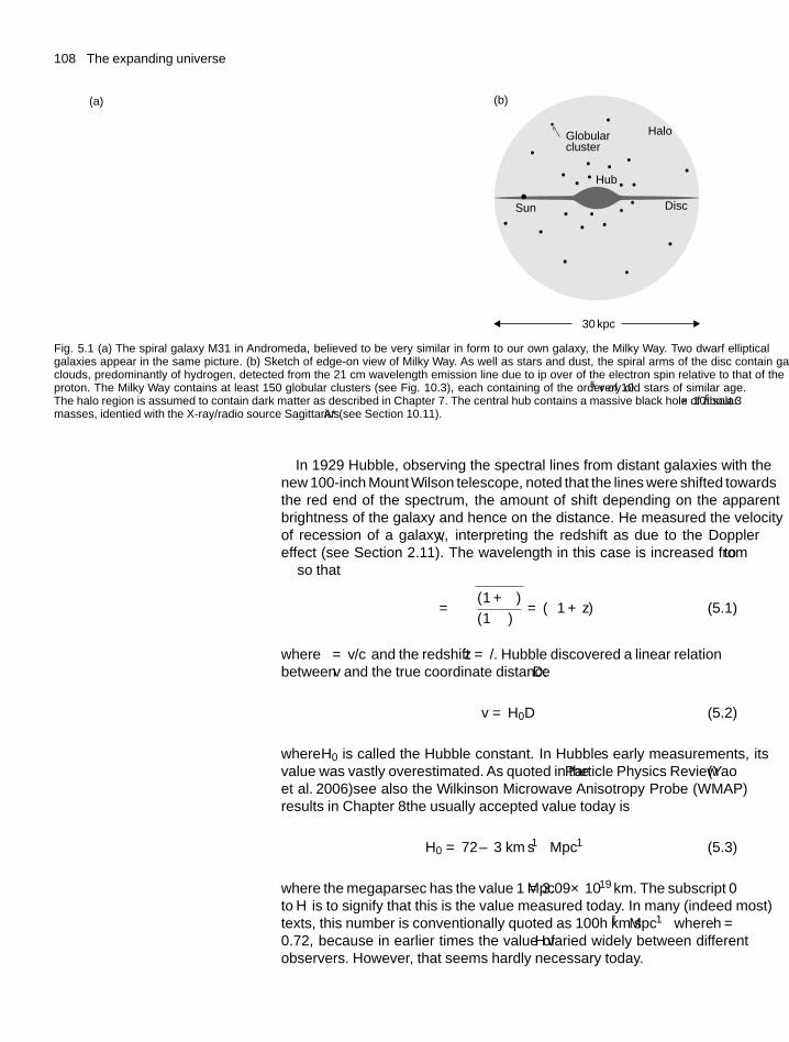
108 The expanding universe
Hub
Disc
Halo
Sun
Globularcluster
30 kpc
(a) (b)
Fig. 5.1 (a) The spiral galaxy M31 in Andromeda, believed to be very similar in form to our own galaxy, the Milky Way. Two dwarf ellipticalgalaxies appear in the same picture. (b) Sketch of edge-on view of Milky Way. As well as stars and dust, the spiral arms of the disc contain gasclouds, predominantly of hydrogen, detected from the 21 cm wavelength emission line due to flip over of the electron spin relative to that of theproton. The Milky Way contains at least 150 globular clusters (see Fig. 10.3), each containing of the order of 105 very old stars of similar age.The halo region is assumed to contain dark matter as described in Chapter 7. The central hub contains a massive black hole of about 3 × 10⁶ solarmasses, identified with the X-ray/radio source Sagittarius A* (see Section 10.11).
In 1929 Hubble, observing the spectral lines from distant galaxies with thenew 100-inch Mount Wilson telescope, noted that the lines were shifted towardsthe red end of the spectrum, the amount of shift depending on the apparentbrightness of the galaxy and hence on the distance. He measured the velocityof recession of a galaxy, v, interpreting the redshift as due to the Dopplereffect (see Section 2.11). The wavelength in this case is increased from λ toλ′ so that
λ′ = λ
√(1 + β)
(1 − β)= λ(1 + z) (5.1)
where β = v/c and the redshift z = �λ/λ. Hubble discovered a linear relationbetween v and the true coordinate distance D:
v = H0D (5.2)
where H0 is called the Hubble constant. In Hubble’s early measurements, itsvalue was vastly overestimated. As quoted in the Particle Physics Review (Yaoet al. 2006)—see also the Wilkinson Microwave Anisotropy Probe (WMAP)results in Chapter 8—the usually accepted value today is
H0 = 72 ± 3 km s−1 Mpc−1 (5.3)
where the megaparsec has the value 1 Mpc = 3.09 × 10¹⁹ km. The subscript ‘0’to H is to signify that this is the value measured today. In many (indeed most)texts, this number is conventionally quoted as 100h km s−1 Mpc−1 where h =0.72, because in earlier times the value of Hvaried widely between differentobservers. However, that seems hardly necessary today.
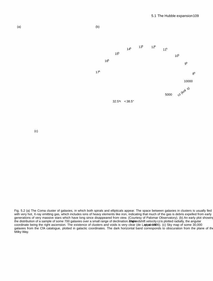
5.1 The Hubble expansion 109
(a) (b)
(c)
17h
16h
15h
14h 13h 12h
11h
10h
9h
8h
10000
5000
32.5° < � < 38.5°
cz (km
–1 s)
Fig. 5.2 (a) The Coma cluster of galaxies, in which both spirals and ellipticals appear. The space between galaxies in clusters is usually filledwith very hot, X-ray emitting gas, which includes ions of heavy elements like iron, indicating that much of the gas is debris expelled from earlygenerations of very massive stars which have long since disappeared from view. (Courtesy of Palomar Observatory). (b) An early plot showingthe distribution of a sample of some 700 galaxies over a small range of declination angle δ. The redshift velocity cz is plotted radially, the angularcoordinate being the right ascension. The existence of clusters and voids is very clear (de Lapparent et al. 1986). (c) Sky map of some 30,000galaxies from the CfA catalogue, plotted in galactic coordinates. The dark horizontal band corresponds to obscuration from the plane of theMilky Way.
110 The expanding universe
Table 5.1 Approximate sizes and masses in theuniverse. (1 parsec = 1 pc = 3.09 × 10¹⁶
m = 3.26 light years)
Radius Mass
Sun 7 × 10⁸ m 2 × 1030 kg = MS
Galaxy 15 kpc 1011MS
Cluster 5 Mpc 1014MS
Supercluster 50 Mpc 1015MS
Universe 4.2 Gpc 1023MS
The interpretation of the redshift in terms of the Doppler effect is permissiblefor the small redshifts of z < 0.003 observed by Hubble. For such nearbygalaxies Newtonian concepts of space and time are applicable. Expanding (5.1)for small values of v/c we get
λ′ ≈ λ(1 + β)
and hencez = v
c(5.4)
However, for distant galaxies and large redshifts, z ≥ 1, the Dopplerformula gives (1 + z) = γ(1 + β), but may not be relevant, since at suchdistances additional, gravitational redshifts, as described in Section 2.3, couldthen become important. The empirical relation observed is therefore of alinear dependence of the redshift on the distance of the galaxy, as given inthe wavelength formula (5.1). The distance is estimated from the apparentbrightness or luminosity, and is therefore called the luminosity distance DL.It is determined from the (supposedly known) intrinsic luminosity L or totalpower radiated by the source (star or galaxy), and the measured energy flux Fat the Earth:
F = L
4πD2L
(5.5)
In fact the astronomers use a logarithmic scale of luminosity, called magnitude,running (perversely) from small values of magnitude for the brightest starsto large values for the faintest. The defining relation between the apparentmagnitude m(z) at redshift z, the so-called absolute magnitude M (equal to thevalue that m would have at DL = 10 pc) and the distance DL in Mpc, is givenby the distance modulus
m(z) − M = 5 log10 DL(z) + 25 (5.6)
In the Hubble diagram, see Fig. 5.3, (m − M ) or log10DL is plotted againstlog10z.
A few words are appropriate here about the establishment of the‘cosmological distance scale’. For nearby sources, distances can be measuredusing parallax, that is the change in direction of the source, relative to moredistant sources as the Earth circulates in solar orbit. (A source at 1 parsecdistance has a parallax of 1 s of arc on a baseline of the Earth–Sun distance of1 a.u.) Over the years, a number of very clever and interlocking methods havebeen used to extend the distance scale. We just have space to mention here oneused to measure the distance (57 kpc) to our nearest neighbour galaxy, the Large
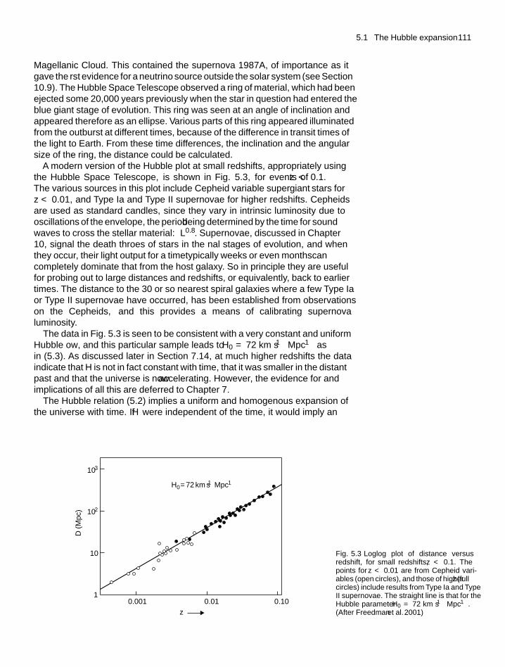
5.1 The Hubble expansion 111
Magellanic Cloud. This contained the supernova 1987A, of importance as itgave the first evidence for a neutrino source outside the solar system (see Section10.9). The Hubble Space Telescope observed a ring of material, which had beenejected some 20,000 years previously when the star in question had entered theblue giant stage of evolution. This ring was seen at an angle of inclination andappeared therefore as an ellipse. Various parts of this ring appeared illuminatedfrom the outburst at different times, because of the difference in transit times ofthe light to Earth. From these time differences, the inclination and the angularsize of the ring, the distance could be calculated.
A modern version of the Hubble plot at small redshifts, appropriately usingthe Hubble Space Telescope, is shown in Fig. 5.3, for events of z < 0.1.The various sources in this plot include Cepheid variable ‘supergiant’ stars forz < 0.01, and Type Ia and Type II supernovae for higher redshifts. Cepheidsare used as ‘standard candles’, since they vary in intrinsic luminosity due tooscillations of the envelope, the period τ being determined by the time for soundwaves to cross the stellar material: τ ∝ L0.8. Supernovae, discussed in Chapter10, signal the death throes of stars in the final stages of evolution, and whenthey occur, their light output for a time—typically weeks or even months—cancompletely dominate that from the host galaxy. So in principle they are usefulfor probing out to large distances and redshifts, or equivalently, back to earliertimes. The distance to the 30 or so nearest spiral galaxies where a few Type Iaor Type II supernovae have occurred, has been established from observationson the Cepheids, and this provides a means of calibrating supernovaluminosity.
The data in Fig. 5.3 is seen to be consistent with a very constant and uniform‘Hubble flow’, and this particular sample leads to H0 = 72 km s−1 Mpc−1 asin (5.3). As discussed later in Section 7.14, at much higher redshifts the dataindicate that H is not in fact constant with time, that it was smaller in the distantpast and that the universe is now accelerating. However, the evidence for andimplications of all this are deferred to Chapter 7.
The Hubble relation (5.2) implies a uniform and homogenous expansion ofthe universe with time. If H were independent of the time, it would imply an
103
102
10
10.001 0.01 0.10
D(M
pc)
H0 = 72 km s–1 Mpc–1
z
Fig. 5.3 Log–log plot of distance versusredshift, for small redshifts, z < 0.1. Thepoints for z < 0.01 are from Cepheid vari-ables (open circles), and those of higher z (fullcircles) include results from Type Ia and TypeII supernovae. The straight line is that for theHubble parameter H0 = 72 km s−1 Mpc−1.(After Freedman et al. 2001)
112 The expanding universe
increase in the size of the universe by a factor e in the so-called Hubble time
tHubble = 1
H0= 13.6 ± 0.5 Gyr (1.36 × 10¹⁰ years) (5.7)
where H0 is the current value of the Hubble parameter. The actual or physicalcoordinate distance D from the Earth, say, to some distant galaxy at time t iswritten as in Section 2.9 as the product
D(t) = r · R(t) (5.8)
where R(t) is the value of the scale parameter and r is the co-moving coordinatedistance measured in a reference frame which is co-moving (i.e. extending) withthe expansion. The quantity r is a time-independent constant (for the distanceto a particular galaxy), while according to the cosmological principle discussedlater, the expansion parameter R(t) is assumed to be the same over all space anddepends only on time, in a way determined by the exact geometry (curvature)of the universe, as indicated in Fig. 5.4. Its value at time t, as compared withthe value today at t = 0, is of course just equal to the reciprocal of the redshiftfactor in (5.1)
R(t) = R(0)
(1 + z)(5.9)
One can normalize R to present-day values by defining the ratio a(t) =R(t)/R(0), and in many texts the parameter a(t) is used to quantify theexpansion. However, in this text we will stick with R. Substituting (5.8) in(5.2) it is seen that the Hubble law is then a statement about the rate of changeof the scale parameter:
R(t) = H R(t) (5.10)
where R = dR/dt. The expansion can be compared with the stretching of thesurface of a balloon under inflation in the two-dimensional case. However,it must be emphasized that the expansion applies only to truly cosmologicaldistances, that is to those between galaxies or galaxy clusters. In the balloonanalogy, the galaxies should be represented by dots or small coins of fixeddiameter stuck on the balloon surface. As the balloon inflates, the galaxiesremain the same size, and the pattern of the galaxies simply expands in size.
The expansion of the universe is usually referred to as the Big Bang, anomenclature originally coined in the 1950s as a term of derision by FredHoyle, who was himself a devotee of the now defunct Steady State theory ofthe universe. How times change! The term Big Bang suggests that a suddenexplosion occurred at a singular point in space–time. Obviously, referredto such an origin, this could reproduce the Hubble relation (5.2), since theparticles of largest velocity will have travelled the farthest from the origin.However, the accepted view of the early universe (before formation of stars andgalaxies at redshifts z < 12) is based on the cosmological principle, namelythat the universe was both isotropic and homogeneous, so that no directionor location was to be preferred over any other, and thus it must appear thesame to all observers no matter where they are. Observationally, the universe isindeed, even today, found to be approximately isotropic on large enough scales,
5.2 Olbers’ paradox 113
and this also implies homogeneity, since a non-homogeneous universe wouldappear isotropic only to a favoured observer stationed at its centre, if it hadspherical symmetry. So the ‘Big Bangs’ occur everywhere at once and theexpansion is the same for all observers irrespective of their location.
Once again, we emphasize that the Hubble ‘expansion of space’ appliesonly to cosmological distances, that is on the scale of intergalactic or largerseparations. It does not imply an increase with time of the size of an atom, orof a planetary system or even of a single galaxy. One can perhaps understandthis on the basis of the smallness of the Hubble constant. The relation v = HDin (5.2) clearly implies an outward acceleration
gHubble = H 2D = 5.10−36D ms−2
where D is in metres. It is left as an exercise to show that for the Earth–Sunsystem, this is only 10−22 of the gravitational acceleration of the Earth insolar orbit, while for a hydrogen atom, the Hubble acceleration is 80 ordersof magnitude less than the inward acceleration of the electron due to theelectric field of the proton. Only when we come to galactic masses M ∼ 1041
kg and intergalactic distance scales D > 1 Mpc do we find the (inward)gravitational acceleration ggrav < 10−14 ms−2 exceeded by gHubble > 10−13
ms−2. Here it should also be pointed out that individual galaxies, just likeindividual stars, have their own ‘peculiar velocities’ (produced by the effectsof nearby gravitating masses) relative to the general outward Hubble flow.For example, our neighbouring galaxy, M31 (see Fig. 5.1) is actually movingtowards the Milky Way. So the Hubble expansion describes a general cosmic-scale behaviour, after peculiar velocities of individual galaxies have beenaveraged out.
What is the cause of the Hubble expansion? That is unknown. We simplyhave to accept it as an empirical fact. The reader is referred to Problem 5.6 foran early proposed model of expansion, demolished by a clever (and even 50years later, still the best) ‘table top’ experiment, set up and completed within10 days of the original proposal being made!
5.2 Olbers’ paradox
In the nineteenth century, Olbers asked the question ‘Why is the sky dark atnight?’ He supposed the universe to be unlimited in extent and filled uniformlywith sources of light (stars). The light flux reaching us from a star at distance rvaries as r−2, while the number of stars in the spherical shell r → r +dr variesas r2dr. Hence the total light flux will increase as r(max), which is infinite inthe model.
There are several reasons why Olbers’arguments are invalid. First, we believethe observable universe is not infinite but has a finite age, and began at a timet0 in the past with the Big Bang which started off the Hubble expansion. Thismeans that light can only reach us from a maximum horizon distance ct0, andthe flux must be finite. A second point is that the light sources (stars) are finitein size, so that nearby sources will block out light from more distant sources.Their light is absorbed exponentially with distance by the intervening stars and
114 The expanding universe
dust. Third, stars only emit light for a finite time t, and the flux from the mostdistant stars will therefore be reduced by a factor t/t0. Finally, the expansion ofthe universe results in an attenuation at large enough redshifts of light of anyparticular frequency; for example, red light will disappear into the infrared andthe flow of light energy will fall off. However, we may remark that, as indicatedbelow, the 2.7 K microwave background radiation which is the cooled and red-shifted remnant of the original expanding fireball of the Big Bang, althoughinvisible to the eye, is just as intense at night time as during the day. So in thissense Olbers was right!
5.3 The Friedmann equation
The evolution of the universe can be described theoretically by the solutionof Einstein’s field equations of general relativity. The ‘Standard Model’ ofpresent day cosmology is the solution proposed by Friedmann–Lemaitre–Robertson–Walker (FLRW for short), which assumes a completely isotropicand homogenous distribution of matter and radiation, behaving like a perfectfrictionless fluid. This assumption of isotropy and homogeneity is a statement ofthe cosmological principle mentioned above. Of course, whatever was the caseat early times in the universe, the matter today does show enormous fluctuationsin density in the form of stars, galaxies and larger structures. But even today theaverage separation between galaxies is of order 100 times their diameter andthe overall expansion of the universe of billions of galaxies on large enoughscales, that is many orders of magnitude larger than the intergalactic separations,still appears to be reasonably well described by the FLRW model. Thus theuniverse is homogeneous in the same sense as is a volume of gas on a scalelarge compared with the intermolecular separation. However, the best evidencefor isotropy and homogeneity on all scales in fact comes from observationsof the cosmic microwave background (CMB) discussed in Section 5.7, whichreflects the distribution of matter and radiation when the universe was onlyabout 380,000 years old (as compared to 14 Gyr today) and long before eitherstars or larger structures had started to form.
The solution for the temporal development of the universe predicted by thismodel was first found by Friedmann (1922), and for the time components ofthe field equations has the form (see also (5.20)):
H 2 =(
R
R
)2
= 8πGρtot
3− kc2
R2(5.11)
where R = R(t) is the expansion parameter in (5.8) and (5.9), ρtot is the totaldensity of matter, radiation, and vacuum energy, as described below, and G isNewton’s gravitational constant. This equation follows when the FLRW metric(2.31) is inserted in the Einstein field equations (2.19).
The term kc2/R2 is the curvature term. As indicated in Chapter 2, one ofthe consequences of general relativity is that, in the presence of gravitatingmasses, the ‘flat’ Euclidean space of special relativity is replaced by curvedspace/time. A light beam going from point A to point B will travel along a pathwhich is an extremum, which is the shortest spatial path length (and also thepath of maximum proper time) called a geodesic. Geodesics are straight lines
5.3 The Friedmann equation 115
in Euclidean space, but in the presence of gravitational fields, the paths arecurved. Of course, this idea is an extension to three dimensions, of the familiartwo-dimensional case in which the shortest path between points on a sphericalsurface is along a great circle.
In the language of particle physics, one might say that space/time appearscurved because photons are deflected (and also retarded, as we knowfrom Section 2.7) by gravitational fields, mediated by graviton exchange.The curvature parameter k can in principle assume values of +1, 0, or−1, corresponding to the curvature k/R2 being positive, zero, or negativerespectively. The two-dimensional analogy for positive or convex curvature isthe surface of a sphere, while that for negative or concave curvature is as in asaddle.
Equation (5.11) has simply been quoted without derivation, but we canunderstand in terms of Newtonian mechanics what it implies in the specialcase where the energy density is dominated by non-relativistic matter. Let usconsider a point mass m being accelerated by gravity at the surface of a sphereof radius D, density ρ, and mass M = 4πD3ρ/3. According to Newtonianmechanics, the assumed spherically symmetric and homogeneous distributionof matter outside of the sphere can make no contribution to the force, whilethe field at the surface is the same as if all the mass were concentrated at thecentre. It turns out that this is also true in general relativity (by a theorem dueto Birkhoff). So the force equation is simply
mD = −mM G
D2(5.12)
where D = d2D/dt2. In this equation, if we express M in terms of D and ρ,factors of r from (5.8) cancel out, and for brevity in what follows we chooseunits such that r = 1 (but must remember that all true cosmological distancesare the product R(t)r). After integrating (5.12) we then get
mR2
2− mM G
R= constant = −mkc2
2(5.13)
If we multiply through by 2/mR2, we obtain an equation in agreement with(5.11), after setting the constant of integration equal to the value given bygeneral relativity. We note that the terms on the left-hand side of (5.13)correspond to the kinetic and potential energies of the mass m, and so the so-called curvature term on the right simply represents the total energy. k = −1corresponds to negative curvature and positive energy, that is to say an openuniverse expanding without limit. For k = −1, R(t) = r · R(t) → c at largeenough values of R. A value k = +1 corresponds to a closed universe withnegative total energy and positive curvature, which reaches a maximum radiusand then collapses. k = 0 is the simplest case, where the kinetic and potentialenergies just balance and the total energy and curvature are both zero. Theuniverse expands for ever but the velocity tends asymptotically to zero at larget. This case is called the flat universe. These three cases are illustrated inFig. 5.4.
Present data indicate that on large scales the universe is extremely close tobeing flat, with k ≈ 0. In that case the constant of integration on the right-handside of (5.13) representing the total energy, potential plus kinetic, is practicallyzero.
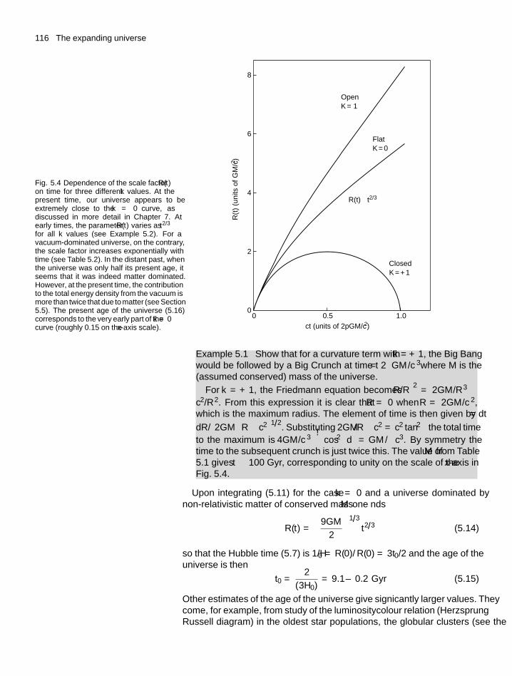
116 The expanding universe
Fig. 5.4 Dependence of the scale factor R(t)on time for three different k values. At thepresent time, our universe appears to beextremely close to the k = 0 curve, asdiscussed in more detail in Chapter 7. Atearly times, the parameter R(t) varies as t2/3
for all k values (see Example 5.2). For avacuum-dominated universe, on the contrary,the scale factor increases exponentially withtime (see Table 5.2). In the distant past, whenthe universe was only half its present age, itseems that it was indeed matter dominated.However, at the present time, the contributionto the total energy density from the vacuum ismore than twice that due to matter (see Section5.5). The present age of the universe (5.16)corresponds to the very early part of the k = 0curve (roughly 0.15 on the x-axis scale).
00 0.5 1.0
FlatK = 0
OpenK = – 1
2
4
6
8
R(t) ∝ t2/3
ClosedK = + 1
ct (units of 2pGM/c2)
R(t
) (u
nits
of
GM
/c2 )
Example 5.1 Show that for a curvature term with k = +1, the Big Bangwould be followed by a Big Crunch at time t = 2πGM /c3where M is the(assumed conserved) mass of the universe.
For k = +1, the Friedmann equation becomes(R/R)2 = 2GM /R3 −
c2/R2. From this expression it is clear that R = 0 when R = 2GM /c2,which is the maximum radius. The element of time is then given by dt =dR/(2GM
/R − c2
)1/2. Substituting 2GM /R−c2 = c2 tan2 θ the total time
to the maximum is(4GM /c3
) ∫cos2 θdθ = GM π/c3. By symmetry the
time to the subsequent crunch is just twice this. The value of M from Table5.1 gives t ∼ 100 Gyr, corresponding to unity on the scale of the x-axis inFig. 5.4.
Upon integrating (5.11) for the case k = 0 and a universe dominated bynon-relativistic matter of conserved mass M one finds
R(t) =(
9GM
2
)1/3
t2/3 (5.14)
so that the Hubble time (5.7) is 1/H0 = R(0)/R(0) = 3t0/2 and the age of theuniverse is then
t0 = 2
(3H0)= 9.1 ± 0.2 Gyr (5.15)
Other estimates of the age of the universe give significantly larger values. Theycome, for example, from study of the luminosity–colour relation (Herzsprung–Russell diagram) in the oldest star populations, the globular clusters (see the
5.4 The sources of energy density 117
caption to Fig. 10.3); from cooling rates of white dwarf stars; and from datingusing isotopic ratios of radioactive elements in the Earth’s crust and in veryold stars. All these estimates straddle an approximate range for the age of theuniverse of
t0 = 14 ± 1 Gyr. (5.16)
The discrepancy between this figure and that for a flat, matter-dominateduniverse (5.15) could be due in principle either to curvature (k �= 0) or tothe existence of a cosmological constant, as discussed below (see (5.23)).However, measurements to be described later indicate that k ≈ 0. In fact asshown in Example 5.3, when account is taken of the effect of the vacuumenergy/cosmological constant, the age of the universe estimated from theHubble parameter is in excellent agreement with the result (5.16). Indeed, it isquite remarkable that completely independent estimates of the age come out inagreement to within 5% or so.
Example 5.2 Find solutions of the Friedmann equation for the case ofa matter-dominated universe of total mass M, and values of k = +1 andk = −1.
The Friedmann equation (5.11) in this case takes the form R2 = 2MG/R−kc2. For k = +1, the solution for R as a function of t has the parametric formof a cycloid curve (i.e. the curve traced out by a point on the circumferenceof a circular disc rolling along a plane):
R = a(1 − cos θ)
t = b(θ − sin θ) (5.17)
as can be verified by substitution. Here, the constants a = MG/kc2 and
b = MG/(kc2)3/2
, and the parameter θ is the angle of rotation of the cycloid.For the case k = −1, the corresponding solution is
R = a(cosh θ − 1)
t = b(sinh θ − θ) (5.18)
with the above values of a and b, and k replaced by |k|. The curves inFig. 5.4 were plotted from these expressions, and the solutions for themaxima and minima in Example 5.1 are found by setting θ = π and 2π in(5.17).
By expanding the above circular functions for small values of θ, it isstraightforward to show that for either k = +1 or −1, the expansionparameter R ∝ t2/3, that is the same as for the case k = 0 in(5.14).
5.4 The sources of energy density
The conservation of energy E in a volume element dV of our perfect cosmicfluid can be expressed as
dE = −PdV
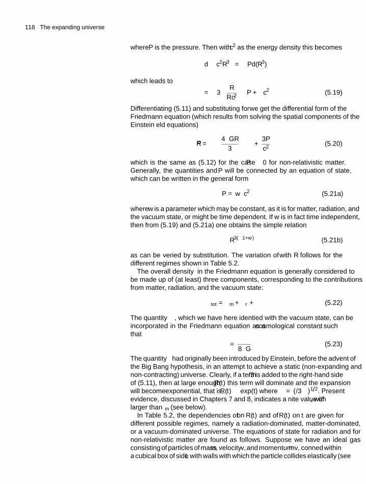
118 The expanding universe
where P is the pressure. Then with ρc2 as the energy density this becomes
d(ρc2R3
)= −Pd(R3)
which leads to
ρ = −3
(R
Rc2
)(P + ρc2
)(5.19)
Differentiating (5.11) and substituting for ρ we get the differential form of theFriedmann equation (which results from solving the spatial components of theEinstein field equations)
R = −(
4πGR
3
)(ρ + 3P
c2
)(5.20)
which is the same as (5.12) for the case P ≈ 0 for non-relativistic matter.Generally, the quantities ρ and P will be connected by an equation of state,which can be written in the general form
P = wρc2 (5.21a)
where w is a parameter which may be constant, as it is for matter, radiation, andthe vacuum state, or might be time dependent. If w is in fact time independent,then from (5.19) and (5.21a) one obtains the simple relation
ρ ∝ R−3(1+w) (5.21b)
as can be verified by substitution. The variation of ρ with R follows for thedifferent regimes shown in Table 5.2.
The overall density ρ in the Friedmann equation is generally considered tobe made up of (at least) three components, corresponding to the contributionsfrom matter, radiation, and the vacuum state:
ρtot = ρm + ρr + ρ� (5.22)
The quantity ρ�, which we have here identified with the vacuum state, can beincorporated in the Friedmann equation as a cosmological constant �, suchthat
ρ� = �
8πG(5.23)
The quantity � had originally been introduced by Einstein, before the advent ofthe Big Bang hypothesis, in an attempt to achieve a static (non-expanding andnon-contracting) universe. Clearly, if a term �/3 is added to the right-hand sideof (5.11), then at large enough R(t) this term will dominate and the expansionwill become exponential, that is, R(t) ∝ exp(αt) where α = (�/3)1/2. Presentevidence, discussed in Chapters 7 and 8, indicates a finite value of �, with ρ�
larger than ρm (see below).In Table 5.2, the dependencies of ρ on R(t) and of R(t) on t are given for
different possible regimes, namely a radiation-dominated, matter-dominated,or a vacuum-dominated universe. The equations of state for radiation and fornon-relativistic matter are found as follows. Suppose we have an ideal gasconsisting of particles of mass m, velocity v, and momentum mv, confined withina cubical box of side L with walls with which the particle collides elastically (see
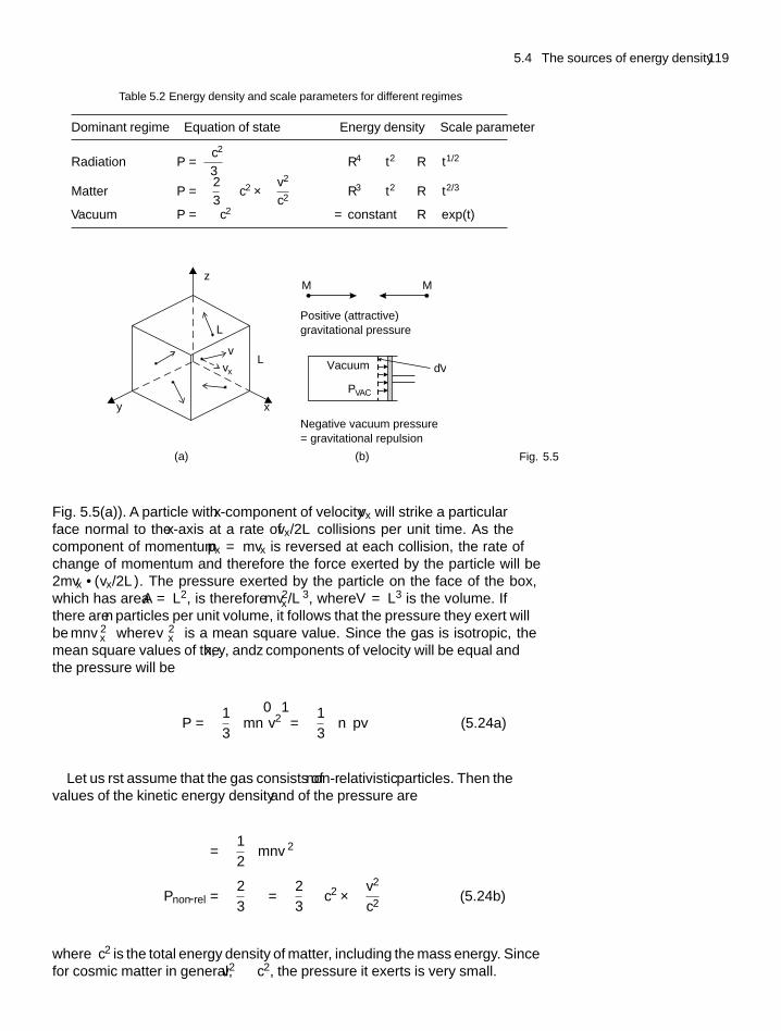
5.4 The sources of energy density 119
Table 5.2 Energy density and scale parameters for different regimes
Dominant regime Equation of state Energy density Scale parameter
Radiation P = ρc2
3ρ ∝ R−4 ∝ t−2 R ∝ t1/2
Matter P =(
2
3
)ρc2 ×
(v2
c2
)ρ ∝ R−3 ∝ t−2 R ∝ t2/3
Vacuum P = −ρc2 ρ = constant R ∝ exp(αt)
z
xy
L
L
v
vx
Positive (attractive)gravitational pressure
Negative vacuum pressure= gravitational repulsion
Vacuum
PVAC
M M
dV
(a) (b) Fig. 5.5
Fig. 5.5(a)). A particle with x-component of velocity vx will strike a particularface normal to the x-axis at a rate of vx/2L collisions per unit time. As thecomponent of momentum px = mvx is reversed at each collision, the rate ofchange of momentum and therefore the force exerted by the particle will be2mvx · (vx/2L). The pressure exerted by the particle on the face of the box,which has area A = L2, is therefore mv2
x/L3, where V = L3 is the volume. Ifthere are n particles per unit volume, it follows that the pressure they exert willbe mn〈v2
x 〉 where 〈v2x 〉 is a mean square value. Since the gas is isotropic, the
mean square values of the x, y, and z components of velocity will be equal andthe pressure will be
P =(
1
3
)mn⟨v2⟩=(
1
3
)n 〈pv〉 (5.24a)
Let us first assume that the gas consists of non-relativistic particles. Then thevalues of the kinetic energy density ε and of the pressure are
ε =(
1
2
)mn〈v2〉
Pnon-rel =(
2
3
)ε =(
2
3
)ρc2 ×
(v2
c2
)(5.24b)
where ρc2 is the total energy density of matter, including the mass energy. Sincefor cosmic matter in general, v2 c2, the pressure it exerts is very small.
120 The expanding universe
If the gas particles have extreme relativistic velocities, then the energy densityand the pressure, usually called the radiation pressure, have the values
ρc2 = n mc2 = n〈pc〉
Prel = ρc2
3(5.25)
That the vacuum may contain an energy density and exert a pressure equivalentto a gravitational repulsion may seem strange, since in classical physics, avacuum is supposed to contain absolutely nothing. However, in quantumfield theory, as has been discussed for the electroweak model in Chapter 3,the Uncertainty Principle actually requires that the vacuum contains virtualparticle–antiparticle pairs which spontaneously appear and disappear, and thevacuum itself is defined, not as nothing but as the state of lowest possible energyof the system. Because the virtual particles carry energy and momentum, if onlyon a temporary basis, general relativity implies that they must be coupled togravitation. Indeed, the measurable effect of such vacuum energy is through itsgravitational influence.
The relation P = −ρc2 for this lowest energy vacuum state can be formallyshown to follow from Lorentz invariance, that is, the requirement that the statemust look the same to all observers, implying also that the energy densitymust have the same constant value everywhere and for all time. A plausibilityargument for the pressure–density relation is as follows. Assume that we havea piston enclosing an isolated cylinder filled with the vacuum state of energydensity ρc2 (see Fig. 5.5(b)). If the piston is withdrawn adiabatically by anelement of volume dV , the extra vacuum energy created will be ρc2 dV , andthis must be supplied by the work done by the vacuum pressure, PdV . Henceby energy conservation P = −ρc2 and from (5.19), ρ = constant.
Note that in (5.20), the deceleration – R is due to the gravitational attractionassociated with the density ρ plus the pressure P. An increase in pressure dueto relativistic particles is proportional to an increase in their energy density andhence in their gravitational potential, through the Einstein relation E = mc2.Thus a negative pressure will correspond to a gravitational repulsion and theexponential expansion indicated in Table 5.2.
5.5 Observed energy densities
For the case k = 0, (5.11) gives a value for the critical density which (today)would just close the universe:
ρc =[
3
(8πG)
]H 2
0 = 9.6 × 10⁻²⁷ kg m−3
andρcc2 = 5.4 ± 0.5 GeV m−3 (5.26)
taking H0 from (5.3). In the second line, we have quoted a critical energydensity, ρcc2. The ratio of the actual density to the critical density is calledthe closure parameter �, which at the present time from (5.11) and for
5.5 Observed energy densities 121
arbitrary k is
� = ρ
ρc= 1 + kc2
[H0R(0)]2(5.27)
One sees that a flat universe with k = 0 will have � = 1 for all values of t. Thedifferent contributions to the total value of � are then, in parallel with (5.22)for radiation, non-relativistic matter, and vacuum densities respectively
� = �r + �m + �� (5.28)
If k �= 0, one can express the curvature term as
�k = ρk
ρc= − kc2
[H0R(0)]2(5.29)
when from (5.27) one obtains
� + �k = �r + �m + �� + �k = 1 (5.30)
At the present time, as described in the next section, the density of themicrowave photon radiation corresponds to �r = 5 × 10⁻⁵ as in (5.54),and is completely negligible in comparison with that of matter, while asindicated below, the vacuum term �� makes a major contribution. In additionto the microwave photon relics of the Big Bang, there are relic neutrinos andantineutrinos (discussed in the following sections), with comparable numberdensity and quantum energy to the photons. Because these neutrinos havemasses comparable with or larger than their kinetic energies today, they arenon-relativistic. However, at early times in the universe when it was muchhotter and radiation-dominated, they were extreme relativistic and so wouldbe included in the radiation term, increasing the radiation energy density bysome 58%.
We now anticipate later results to be described more fully in Chapter 8.Apart from a very small energy density contribution in microwave photons andneutrinos discussed in Sections 5.8–5.11, the energy density of the universetoday is made up of several components as follows:
1. For luminous baryonic matter (i.e. visible protons, neutrons, and nuclei)in the form of stars, gas, and dust it is found that
ρlum = 9 × 10⁻²⁹ kg m−3
or�lum = 0.01 (5.31)
2. The total density of baryons, visible or invisible, as inferred from themodel of nucleosynthesis described in the next chapter, is about 0.26baryons m−3, or an energy density
ρb = 4.0 × 10⁻²⁸ kg m−3
and�b = 0.042 ± 0.004 (5.32)
122 The expanding universe
3. The total matter density, as inferred from the gravitational potentialenergy deduced from galactic rotation curves (see Section 7.2) and thekinematics of large-scale structures in the universe (see Section 8.9) isfound to be
ρm = 2.2 × 10⁻²⁷ kg m−3
and�m = 0.24 ± 0.03 (5.33)
4. The dark (or vacuum) energy density can be measured from an observedcurvature in the Hubble plot, obtained from study of Type 1Asupernovaeat large redshifts (see Section 7.14). It may also be inferred from theposition of the ‘acoustic peaks’ in the angular power spectrum of thetemperature fluctuations in the microwave radiation (see Sections 8.13–8.16) measuring the total density
�total = 1.0 ± 0.02 (5.34)
These results and (5.33) indicate a value for the dark energy density of
�� = 0.76 ± 0.05 (5.35)
We should note here that in many texts, H0 is specified as 100h km s−1 Mpc−1
where h = 0.72. In that case the critical density in (5.26) would be quoted asρc/h2 and the value of the closure parameter as �h2, where h2 = 0.52.
There are several important conclusions from equations (5.28) to (5.35).First, the value of unity in (5.34) for the total closure parameter indicates a flatuniverse (k = 0), as is predicted by the inflationary model of the very earlyuniverse described in Chapter 8. Next, we note that most of the baryonic matteris non-luminous, and that baryons, visible or invisible, account for only a smallfraction, of order 17%, of the total matter. The bulk is ascribed to dark matter,as discussed in detail in Chapter 7. The nature of such dark matter is presentlyunknown. Finally, it appears that at the present epoch, the bulk of the energydensity is in the form of dark energy. Here, as in Chapter 7, we have identifiedthis dark energy with vacuum energy and a ‘�’ subscript, but other possibilitieshave been proposed, such as a fifth type of fundamental interaction, with thedark energy density being a function of time. Like dark matter, the source ofthe dark energy is unknown at the present time. In fact it has been possible tomeasure the parameter w = P/ρc2 in the equation of state (5.21) for the darkenergy term, with the present result
w(dark energy) = −0.97 ± 0.08 (5.36)
consistent with the value -1 for a simple vacuum. However, the crucial andimportant fact to bear in mind here is that at the present time, the nature of 95%of the energy density of the universe is completely unknown.
Other possibilities, instead of dark matter and/or dark energy, are ofdeviations from Newton’s inverse square law of gravitation for very largecosmic distances. Such deviations from conventional gravity have beenrepeatedly proposed over the years, but at present there seems to be absolutelyno evidence in their favour. Indeed, instances have been found of galaxiespassing through one another, in which visible matter and dark matter (detected
5.6 The age and size of the universe 123
from its gravitational influence via gravitational lensing) are clearly separated,presumably because the visible matter undergoes electromagnetic interactions,while the dark matter is only weakly interacting. It is also perhaps worth statinghere that as a result of recent measurements, the postulated partition of energyamong the various components described above has changed dramatically overthe last decade or so. Twenty years ago, it was thought that vacuum energywould make only a minor contribution, and that the value � ∼ 1 would bemade up largely of dark matter.
Finally, we may note that it appears somewhat miraculous that, of all theconceivable values of �tot, the one observed today appears to be very close tothe value of unity expected for a flat universe with zero total energy and zerocurvature. As stated before, of all the different numbers required to describethe universe, this zero value appears to be the only natural one.
5.6 The age and size of the universe
An estimate of the age of the universe, including all the sources of energydensity, can be made as follows. From (5.11) and (5.27) to (5.30) the Hubbleparameter at time t is given by
H (t)2 = (8πG/3) [ρm(t) + ρr(t) + ρ�(t) + ρk(t)]
= H 20 [�m(t) + �r(t) + ��(t) + �k(t)]
= H 20
[�m(0)(1 + z)3 + �r(0)(1 + z)4 + ��(0) + �k(0)(1 + z)2
](5.37)
where we have used the fact that R(0)/R(t) = (1 + z) from (5.9), and that,as shown in Section 5.8 and Table 5.2, matter, radiation, and curvature termsvary as 1/R3, 1/R4, and 1/R2 respectively. The vacuum energy, by definition,is independent of z, while �k(0) = −kc2/(R0H0)
2 as in (5.29). Furthermore,from (5.9)
H =(
1
R
)dR
dt= −
(dz/
dt
(1 + z)
)and hence
dt = − dz
[(1 + z)H ] (5.38)
We integrate to obtain the interval from the time t when the redshift was z, tothe present time, t0, when z = 0:
t0 − t = 1
H0
∫dz
(1 + z)[�m(0)(1 + z)3 + �r(1 + z)4
+��(0) + �k(0)(1 + z)2]1/2
(5.39)
The age is found by setting the upper limit as z = ∞ at t = 0. In the generalcase this integral has to be evaluated numerically, but there are a few caseswhere analytical solutions are possible, for example, when the radiation termcan be neglected and either �� = 0 or �k = 0, as shown in Example 5.3 and inProblem (5.11), and illustrated in Fig. 5.6. The result (5.15) obviously follows
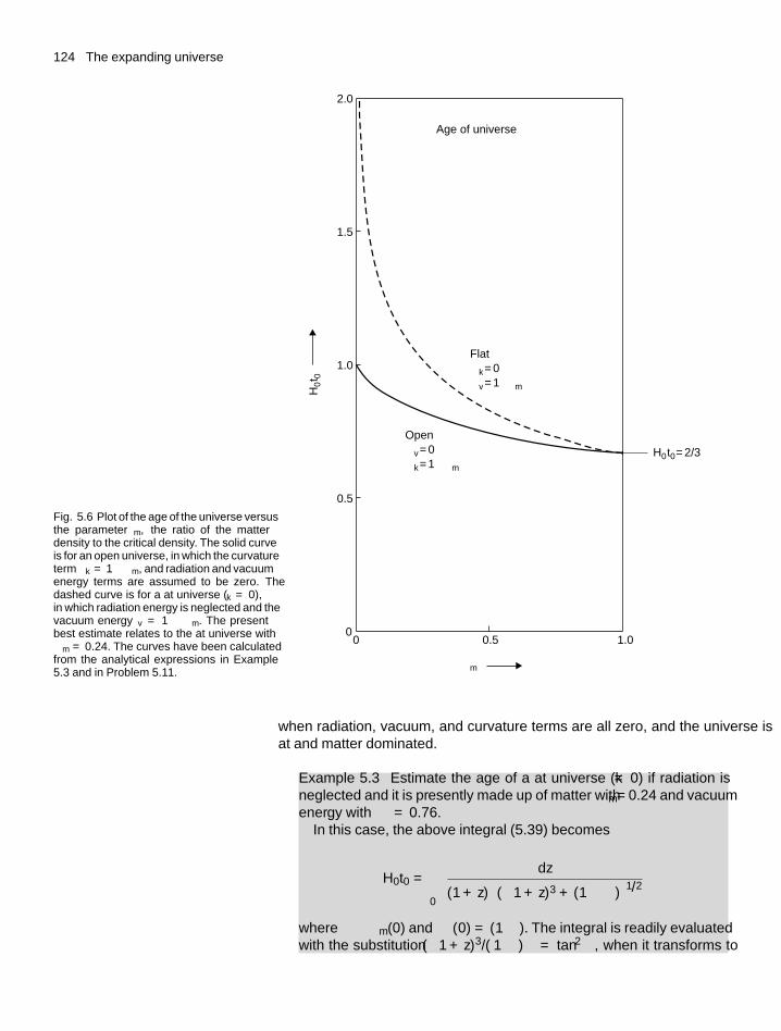
124 The expanding universe
Fig. 5.6 Plot of the age of the universe versusthe parameter �m, the ratio of the matterdensity to the critical density. The solid curveis for an open universe, in which the curvatureterm �k = 1−�m, and radiation and vacuumenergy terms are assumed to be zero. Thedashed curve is for a flat universe (�k = 0),in which radiation energy is neglected and thevacuum energy �v = 1 − �m. The presentbest estimate relates to the flat universe with�m = 0.24. The curves have been calculatedfrom the analytical expressions in Example5.3 and in Problem 5.11.
FlatΩk = 0Ωv = 1– Ωm
OpenΩv = 0Ωk = 1 – Ωm
H0 t0 = 2/3
H0t 0
Ωm
Age of universe
2.0
1.5
1.0
0.5
00 0.5 1.0
when radiation, vacuum, and curvature terms are all zero, and the universe isflat and matter dominated.
Example 5.3 Estimate the age of a flat universe (k = 0) if radiation isneglected and it is presently made up of matter with �m= 0.24 and vacuumenergy with �� = 0.76.
In this case, the above integral (5.39) becomes
H0t0 =∞∫
0
dz
(1 + z)[�(1 + z)3 + (1 − �)
]1/2
where � ≡ �m(0) and ��(0) = (1 − �). The integral is readily evaluatedwith the substitution �(1 + z)3/(1 − �) = tan2 θ , when it transforms to
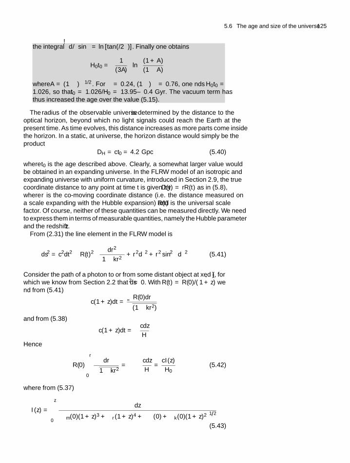
5.6 The age and size of the universe 125
the integral∫
dθ/sin θ = ln [tan (θ/2)]. Finally one obtains
H0t0 =[
1
(3A)
]ln
[(1 + A)
(1 − A)
]where A = (1 − �)1/2. For � = 0.24, (1 − �) = 0.76, one finds H0t0 =1.026, so that t0 = 1.026/H0 = 13.95 ± 0.4 Gyr. The vacuum term hasthus increased the age over the value (5.15).
The radius of the observable universe is determined by the distance to theoptical horizon, beyond which no light signals could reach the Earth at thepresent time. As time evolves, this distance increases as more parts come insidethe horizon. In a static, flat universe, the horizon distance would simply be theproduct
DH = ct0 = 4.2 Gpc (5.40)
where t0 is the age described above. Clearly, a somewhat larger value wouldbe obtained in an expanding universe. In the FLRW model of an isotropic andexpanding universe with uniform curvature, introduced in Section 2.9, the truecoordinate distance to any point at time t is given by D(t) = rR(t) as in (5.8),where r is the co-moving coordinate distance (i.e. the distance measured ona scale expanding with the Hubble expansion) and R(t) is the universal scalefactor. Of course, neither of these quantities can be measured directly. We needto express them in terms of measurable quantities, namely the Hubble parameterand the redshift z.
From (2.31) the line element in the FLRW model is
ds2 = c2dt2 − R(t)2
[dr2(
1 − kr2) + r2dθ2 + r2 sin2 θ dϕ2
](5.41)
Consider the path of a photon to or from some distant object at fixed (θ, ϕ), forwhich we know from Section 2.2 that ds2 = 0. With R(t) = R(0)/(1 + z) wefind from (5.41)
c(1 + z)dt = R(0)dr√(1 − kr2)
and from (5.38)
c(1 + z)dt = −cdz
H
Hence
R(0)
r∫0
dr√1 − kr2
= −∫
cdz
H= cI(z)
H0(5.42)
where from (5.37)
I(z) =z∫
0
dz[�m(0)(1 + z)3 + �r(1 + z)4 + ��(0) + �k(0)(1 + z)2
]1/2
(5.43)
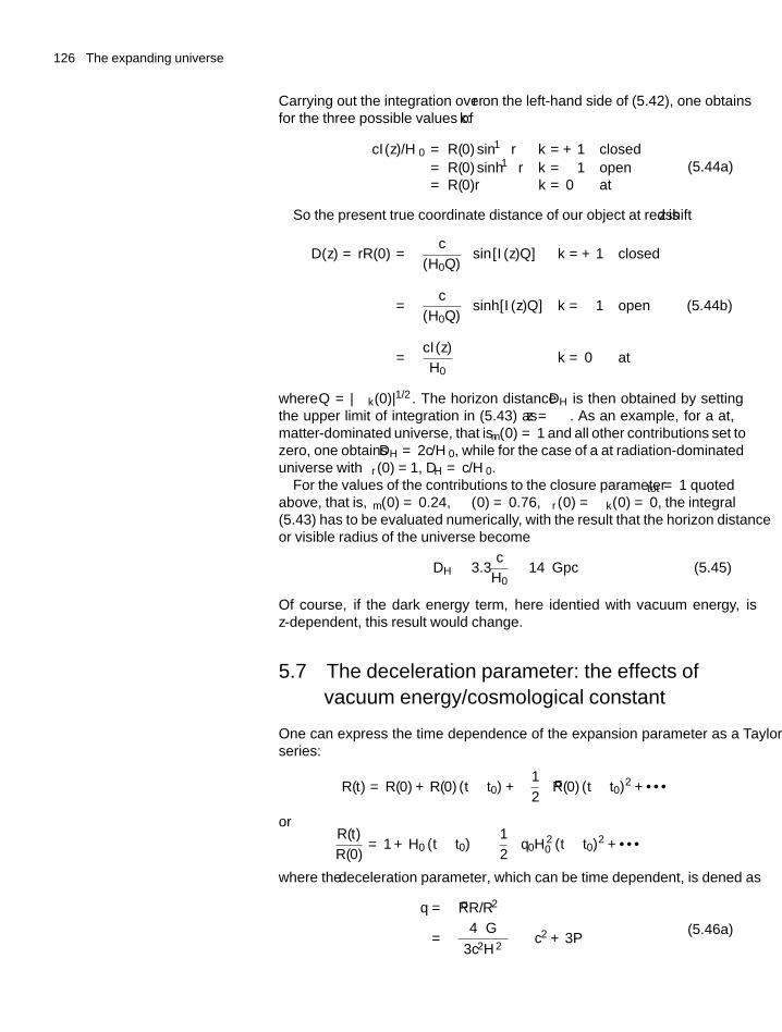
126 The expanding universe
Carrying out the integration over r on the left-hand side of (5.42), one obtainsfor the three possible values of k:
cI(z)/H0 = R(0) sin−1 r k = +1 closed= R(0) sinh−1 r k = −1 open= R(0)r k = 0 flat
(5.44a)
So the present true coordinate distance of our object at redshift z is
D(z) = rR(0) =[
c
(H0Q)
]sin [I(z)Q] k = +1 closed
=[
c
(H0Q)
]sinh [I(z)Q] k = −1 open
=[
cI(z)
H0
]k = 0 flat
(5.44b)
where Q = |�k (0)|1/2. The horizon distance DH is then obtained by settingthe upper limit of integration in (5.43) as z = ∞. As an example, for a flat,matter-dominated universe, that is, �m(0) = 1 and all other contributions set tozero, one obtains DH = 2c/H0, while for the case of a flat radiation-dominateduniverse with �r(0) = 1, DH = c/H0.
For the values of the contributions to the closure parameter �tot = 1 quotedabove, that is, �m(0) = 0.24, ��(0) = 0.76, �r(0) = �k(0) = 0, the integral(5.43) has to be evaluated numerically, with the result that the horizon distanceor visible radius of the universe become
DH ∼ 3.3c
H0∼ 14 Gpc (5.45)
Of course, if the dark energy term, here identified with vacuum energy, isz-dependent, this result would change.
5.7 The deceleration parameter: the effects ofvacuum energy/cosmological constant
One can express the time dependence of the expansion parameter as a Taylorseries:
R(t) = R(0) + R(0) (t − t0) +(
1
2
)R(0) (t − t0)
2 + · · ·
orR(t)
R(0)= 1 + H0 (t − t0) −
(1
2
)q0H 2
0 (t − t0)2 + · · ·
where the deceleration parameter, which can be time dependent, is defined as
q = −RR/R2
=[
4πG(3c2H 2
)] [ρc2 + 3P] (5.46a)
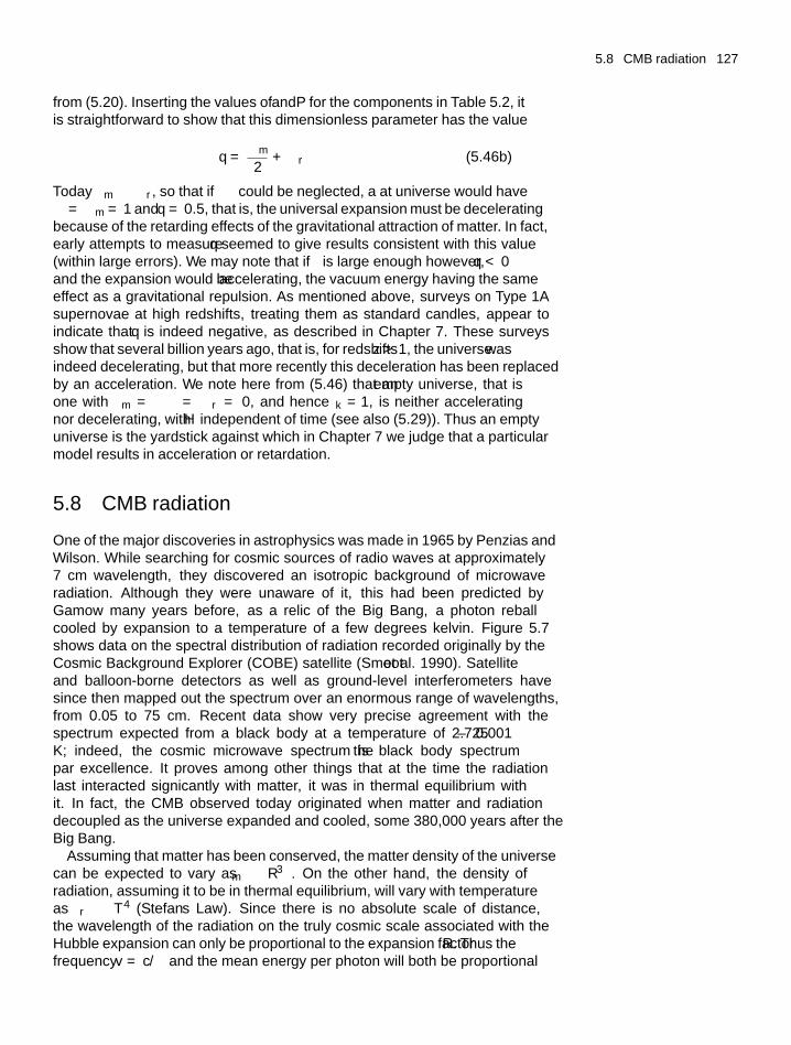
5.8 CMB radiation 127
from (5.20). Inserting the values of ρ and P for the components in Table 5.2, itis straightforward to show that this dimensionless parameter has the value
q = �m
2+ �r − �� (5.46b)
Today �m � �r , so that if �� could be neglected, a flat universe would have� = �m = 1 and q = 0.5, that is, the universal expansion must be deceleratingbecause of the retarding effects of the gravitational attraction of matter. In fact,early attempts to measure q seemed to give results consistent with this value(within large errors). We may note that if �� is large enough however, q < 0and the expansion would be accelerating, the vacuum energy having the sameeffect as a gravitational repulsion. As mentioned above, surveys on Type 1Asupernovae at high redshifts, treating them as ‘standard candles’, appear toindicate that q is indeed negative, as described in Chapter 7. These surveysshow that several billion years ago, that is, for redshifts z > 1, the universe wasindeed decelerating, but that more recently this deceleration has been replacedby an acceleration. We note here from (5.46) that an empty universe, that isone with �m = �� = �r = 0, and hence �k = 1, is neither acceleratingnor decelerating, with H independent of time (see also (5.29)). Thus an emptyuniverse is the yardstick against which in Chapter 7 we judge that a particularmodel results in acceleration or retardation.
5.8 CMB radiation
One of the major discoveries in astrophysics was made in 1965 by Penzias andWilson. While searching for cosmic sources of radio waves at approximately7 cm wavelength, they discovered an isotropic background of microwaveradiation. Although they were unaware of it, this had been predicted byGamow many years before, as a relic of the Big Bang, a photon fireballcooled by expansion to a temperature of a few degrees kelvin. Figure 5.7shows data on the spectral distribution of radiation recorded originally by theCosmic Background Explorer (COBE) satellite (Smoot et al. 1990). Satelliteand balloon-borne detectors as well as ground-level interferometers havesince then mapped out the spectrum over an enormous range of wavelengths,from 0.05 to 75 cm. Recent data show very precise agreement with thespectrum expected from a black body at a temperature of 2.725 ± 0.001K; indeed, the cosmic microwave spectrum is the black body spectrumpar excellence. It proves among other things that at the time the radiationlast interacted significantly with matter, it was in thermal equilibrium withit. In fact, the CMB observed today originated when matter and radiationdecoupled as the universe expanded and cooled, some 380,000 years after theBig Bang.
Assuming that matter has been conserved, the matter density of the universecan be expected to vary as ρm ∝ R−3. On the other hand, the density ofradiation, assuming it to be in thermal equilibrium, will vary with temperatureas ρr ∝ T 4 (Stefan’s Law). Since there is no absolute scale of distance,the wavelength of the radiation on the truly cosmic scale associated with theHubble expansion can only be proportional to the expansion factor R. Thus thefrequency v = c/λ and the mean energy per photon will both be proportional
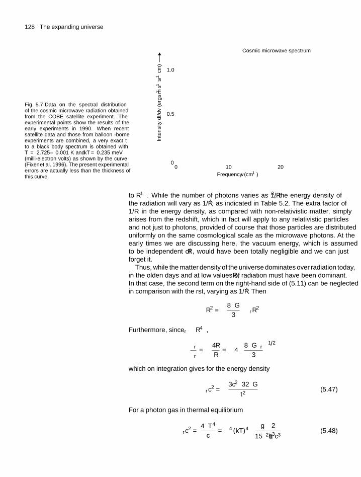
128 The expanding universe
Fig. 5.7 Data on the spectral distributionof the cosmic microwave radiation obtainedfrom the COBE satellite experiment. Theexperimental points show the results of theearly experiments in 1990. When recentsatellite data and those from balloon -borneexperiments are combined, a very exact fitto a black body spectrum is obtained withT = 2.725 ± 0.001 K and kT = 0.235 meV(milli-electron volts) as shown by the curve(Fixen et al. 1996). The present experimentalerrors are actually less than the thickness ofthis curve.
Cosmic microwave spectrum
Inte
nsity
dI/
dv (
ergs
m–2
s–1sr
–1cm
)0
0 10Frequency v (cm–1)
20
0.5
1.0
to R−1. While the number of photons varies as 1/R3, the energy density ofthe radiation will vary as 1/R4, as indicated in Table 5.2. The extra factor of1/R in the energy density, as compared with non-relativistic matter, simplyarises from the redshift, which in fact will apply to any relativistic particlesand not just to photons, provided of course that those particles are distributeduniformly on the same cosmological scale as the microwave photons. At theearly times we are discussing here, the vacuum energy, which is assumedto be independent of R, would have been totally negligible and we can justforget it.
Thus, while the matter density of the universe dominates over radiation today,in the olden days and at low values of R, radiation must have been dominant.In that case, the second term on the right-hand side of (5.11) can be neglectedin comparison with the first, varying as 1/R4. Then
R2 =(
8πG
3
)ρrR2
Furthermore, since ρr ∝ R−4,
ρr
ρr= −4R
R= −4
(8πGρr
3
)1/2
which on integration gives for the energy density
ρrc2 =(
3c2/
32πG
t2
)(5.47)
For a photon gas in thermal equilibrium
ρrc2 = 4σT 4
c= π4 (kT )4
(gγ
/2
15π2h3c3
)(5.48)
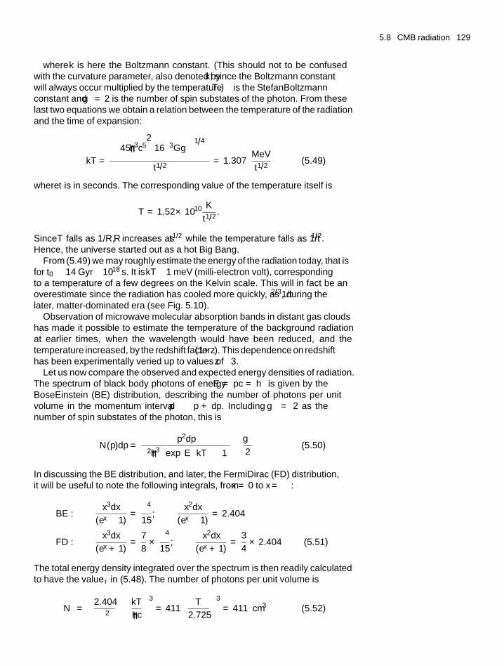
5.8 CMB radiation 129
where k is here the Boltzmann constant. (This should not to be confusedwith the curvature parameter, also denoted by k; since the Boltzmann constantwill always occur multiplied by the temperature T .) σ is the Stefan–Boltzmannconstant and gγ = 2 is the number of spin substates of the photon. From theselast two equations we obtain a relation between the temperature of the radiationand the time of expansion:
kT =
[(45h3c5
/16π3Ggγ
)1/4]
t1/2= 1.307
MeV
t1/2(5.49)
where t is in seconds. The corresponding value of the temperature itself is
T = 1.52 × 10¹⁰ K
t1/2.
Since T falls as 1/R, R increases as t1/2 while the temperature falls as 1/t1/2.Hence, the universe started out as a hot Big Bang.
From (5.49) we may roughly estimate the energy of the radiation today, that isfor t0 ∼ 14 Gyr ∼ 1018 s. It is kT ∼ 1 meV (milli-electron volt), correspondingto a temperature of a few degrees on the Kelvin scale. This will in fact be anoverestimate since the radiation has cooled more quickly, as 1/t2/3, during thelater, matter-dominated era (see Fig. 5.10).
Observation of microwave molecular absorption bands in distant gas cloudshas made it possible to estimate the temperature of the background radiationat earlier times, when the wavelength would have been reduced, and thetemperature increased, by the redshift factor (1+z). This dependence on redshifthas been experimentally verified up to values of z ≈ 3.
Let us now compare the observed and expected energy densities of radiation.The spectrum of black body photons of energy E = pc = hν is given by theBose–Einstein (BE) distribution, describing the number of photons per unitvolume in the momentum interval p → p + dp. Including gγ = 2 as thenumber of spin substates of the photon, this is
N (p)dp = p2dp
π2h3 {exp(E/
kT)− 1
} (gγ
2
)(5.50)
In discussing the BE distribution, and later, the Fermi–Dirac (FD) distribution,it will be useful to note the following integrals, from x = 0 to x = ∞:
BE :∫
x3dx
(ex − 1)= π4
15;∫
x2dx
(ex − 1)= 2.404
FD :∫
x3dx
(ex + 1)= 7
8× π4
15;∫
x2dx
(ex + 1)= 3
4× 2.404 (5.51)
The total energy density integrated over the spectrum is then readily calculatedto have the value ρr in (5.48). The number of photons per unit volume is
Nγ =(
2.404
π2
)(kT
hc
)3
= 411
(T
2.725
)3
= 411 cm−3 (5.52)
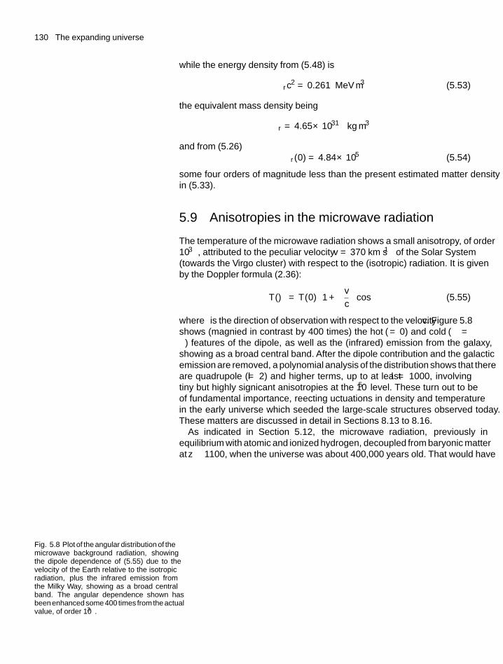
130 The expanding universe
while the energy density from (5.48) is
ρrc2 = 0.261 MeV m−3 (5.53)
the equivalent mass density being
ρr = 4.65 × 10⁻³¹ kg m−3
and from (5.26)�r(0) = 4.84 × 10⁻⁵ (5.54)
some four orders of magnitude less than the present estimated matter densityin (5.33).
5.9 Anisotropies in the microwave radiation
The temperature of the microwave radiation shows a small anisotropy, of order10−3, attributed to the ‘peculiar velocity’ v = 370 km s−1 of the Solar System(towards the Virgo cluster) with respect to the (isotropic) radiation. It is givenby the Doppler formula (2.36):
T (θ) = T (0)[1 +(v
c
)cos θ]
(5.55)
where θ is the direction of observation with respect to the velocity v. Figure 5.8shows (magnified in contrast by 400 times) the ‘hot’ (θ = 0) and ‘cold’ (θ =π) features of the dipole, as well as the (infrared) emission from the galaxy,showing as a broad central band. After the dipole contribution and the galacticemission are removed, a polynomial analysis of the distribution shows that thereare quadrupole (l = 2) and higher terms, up to at least l = 1000, involvingtiny but highly significant anisotropies at the 10−5 level. These turn out to beof fundamental importance, reflecting fluctuations in density and temperaturein the early universe which seeded the large-scale structures observed today.These matters are discussed in detail in Sections 8.13 to 8.16.
As indicated in Section 5.12, the microwave radiation, previously inequilibrium with atomic and ionized hydrogen, decoupled from baryonic matterat z ∼ 1100, when the universe was about 400,000 years old. That would have
Fig. 5.8 Plot of the angular distribution of themicrowave background radiation, showingthe dipole dependence of (5.55) due to thevelocity of the Earth relative to the isotropicradiation, plus the infrared emission fromthe Milky Way, showing as a broad centralband. The angular dependence shown hasbeen enhanced some 400 times from the actualvalue, of order 10−3.
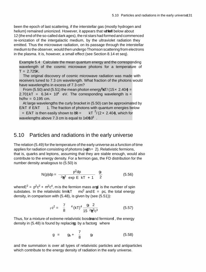
5.10 Particles and radiations in the early universe 131
been the epoch of ‘last scattering’, if the interstellar gas (mostly hydrogen andhelium) remained unionized. However, it appears that when z fell below about12 (the end of the so-called dark ages), the first stars had formed and commencedre-ionization of the intergalactic medium, by the ultraviolet radiation theyemitted. Thus the microwave radiation, on its passage through the interstellarmedium to the observer, would then undergo Thomson scattering from electronsin the plasma. It is, however, a small effect (see Section 8.14 et seq).
Example 5.4 Calculate the mean quantum energy and the correspondingwavelength of the cosmic microwave photons for a temperature ofT = 2.725 K.
The original discovery of cosmic microwave radiation was made withreceivers tuned to 7.3 cm wavelength. What fraction of the photons wouldhave wavelengths in excess of 7.3 cm?
From (5.50) and (5.51) the mean photon energy is π4kT/(15 × 2.404) =2.701 kT = 6.34 × 10⁻⁴ eV. The corresponding wavelength is λ =hc/hv = 0.195 cm.
At large wavelengths the curly bracket in (5.50) can be approximated byE/kT if E/kT 1. The fraction of photons with quantum energies belowε = E/kT is then easily shown to be F = (ε/kT
)2/(2 × 2.404), which for
wavelengths above 7.3 cm is equal to 1.06 × 10⁻³.
5.10 Particles and radiations in the early universe
The relation (5.49) for the temperature of the early universe as a function of timeapplies for radiation consisting of photons (with gγ = 2). Relativistic fermions,that is, quarks and leptons, assuming that they are stable enough, would alsocontribute to the energy density. For a fermion gas, the FD distribution for thenumber density analogous to (5.50) is
N (p)dp = p2dp
π2h3 {exp(E/
kT)+ 1
} (gf
2
)(5.56)
where E2 = p2c2 + m2c4, m is the fermion mass and gf is the number of spinsubstates. In the relativistic limit, kT � mc2 and E = pc, the total energydensity, in comparison with (5.48), is given by (see (5.51)):
ρf c2 =(
7
8
)π4 (kT )4
(gf/
2)
15π2h3c3(5.57)
Thus, for a mixture of extreme relativistic bosons b and fermions f , the energydensity in (5.48) is found by replacing gγ by a factor g∗ where
g∗ =∑
gb +(
7
8
)∑gf (5.58)
and the summation is over all types of relativistic particles and antiparticleswhich contribute to the energy density of radiation in the early universe.
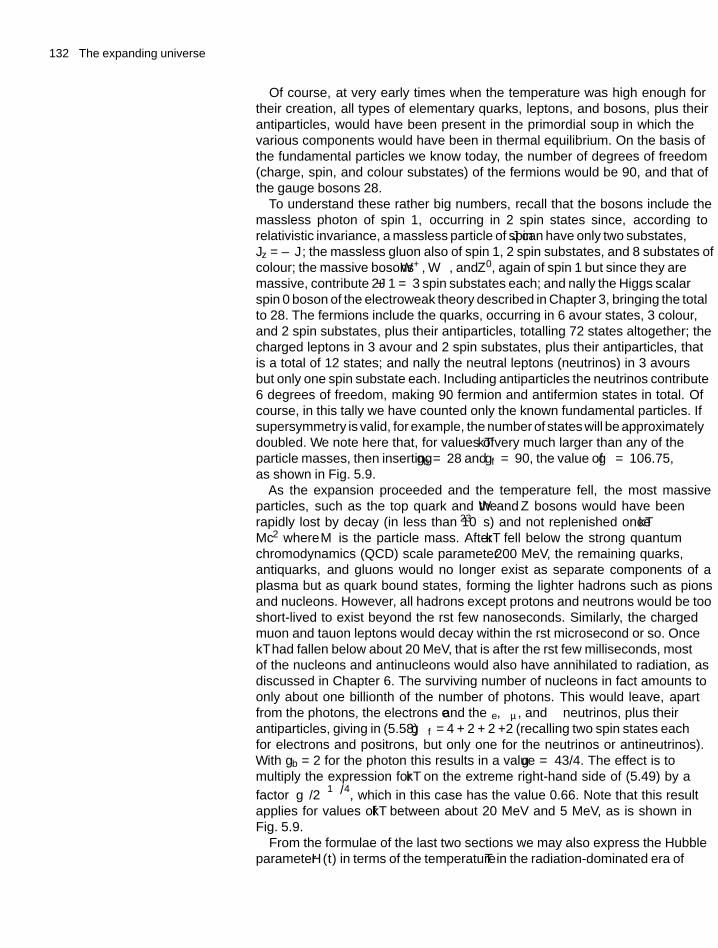
132 The expanding universe
Of course, at very early times when the temperature was high enough fortheir creation, all types of elementary quarks, leptons, and bosons, plus theirantiparticles, would have been present in the primordial ‘soup’ in which thevarious components would have been in thermal equilibrium. On the basis ofthe fundamental particles we know today, the number of degrees of freedom(charge, spin, and colour substates) of the fermions would be 90, and that ofthe gauge bosons 28.
To understand these rather big numbers, recall that the bosons include themassless photon of spin 1, occurring in 2 spin states since, according torelativistic invariance, a massless particle of spin J can have only two substates,Jz = ±J ; the massless gluon also of spin 1, 2 spin substates, and 8 substates ofcolour; the massive bosons W +, W −, and Z0, again of spin 1 but since they aremassive, contribute 2J +1 = 3 spin substates each; and finally the Higgs scalarspin 0 boson of the electroweak theory described in Chapter 3, bringing the totalto 28. The fermions include the quarks, occurring in 6 flavour states, 3 colour,and 2 spin substates, plus their antiparticles, totalling 72 states altogether; thecharged leptons in 3 flavour and 2 spin substates, plus their antiparticles, thatis a total of 12 states; and finally the neutral leptons (neutrinos) in 3 flavoursbut only one spin substate each. Including antiparticles the neutrinos contribute6 degrees of freedom, making 90 fermion and antifermion states in total. Ofcourse, in this tally we have counted only the known fundamental particles. Ifsupersymmetry is valid, for example, the number of states will be approximatelydoubled. We note here that, for values of kT very much larger than any of theparticle masses, then inserting gb = 28 and gf = 90, the value of g∗ = 106.75,as shown in Fig. 5.9.
As the expansion proceeded and the temperature fell, the most massiveparticles, such as the top quark and the W and Z bosons would have beenrapidly lost by decay (in less than 10−23 s) and not replenished once kT Mc2 where M is the particle mass. After kT fell below the strong quantumchromodynamics (QCD) scale parameter ∼ 200 MeV, the remaining quarks,antiquarks, and gluons would no longer exist as separate components of aplasma but as quark bound states, forming the lighter hadrons such as pionsand nucleons. However, all hadrons except protons and neutrons would be tooshort-lived to exist beyond the first few nanoseconds. Similarly, the chargedmuon and tauon leptons would decay within the first microsecond or so. OncekT had fallen below about 20 MeV, that is after the first few milliseconds, mostof the nucleons and antinucleons would also have annihilated to radiation, asdiscussed in Chapter 6. The surviving number of nucleons in fact amounts toonly about one billionth of the number of photons. This would leave, apartfrom the photons, the electrons e− and the νe, νμ, and ντ neutrinos, plus theirantiparticles, giving in (5.58) �gf = 4 + 2 + 2 +2 (recalling two spin states eachfor electrons and positrons, but only one for the neutrinos or antineutrinos).With gb = 2 for the photon this results in a value g∗ = 43/4. The effect is tomultiply the expression for kT on the extreme right-hand side of (5.49) by a
factor(g∗/2)−1/4
, which in this case has the value 0.66. Note that this resultapplies for values of kT between about 20 MeV and 5 MeV, as is shown inFig. 5.9.
From the formulae of the last two sections we may also express the Hubbleparameter H (t) in terms of the temperature T in the radiation-dominated era of
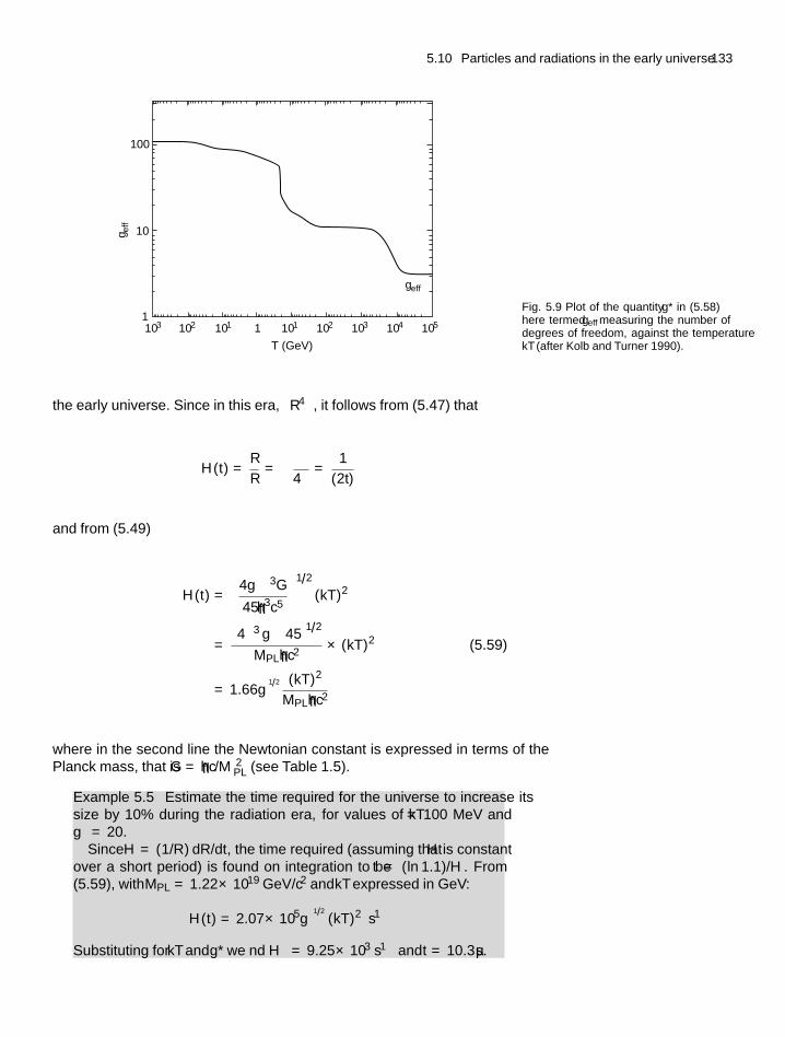
5.10 Particles and radiations in the early universe 133
100
10
1103 102 101 10–1 10–2 10–3 10–4 10–51
T (GeV)
geff
g eff
Fig. 5.9 Plot of the quantity g* in (5.58)—here termed geff —measuring the number ofdegrees of freedom, against the temperaturekT (after Kolb and Turner 1990).
the early universe. Since in this era, ρ ∝ R−4, it follows from (5.47) that
H (t) = R
R= − ρ
4ρ= 1
(2t)
and from (5.49)
H (t) =[
4g∗π3G
45h3c5
]1/2
(kT )2
=(4π3 g∗/45
)1/2
MPLhc2× (kT )2 (5.59)
= 1.66g∗1/2 (kT )2
MPLhc2
where in the second line the Newtonian constant is expressed in terms of thePlanck mass, that is G = hc/M 2
PL (see Table 1.5).
Example 5.5 Estimate the time required for the universe to increase itssize by 10% during the radiation era, for values of kT = 100 MeV andg∗ = 20.
Since H = (1/R) dR/dt, the time required (assuming that H is constantover a short period) is found on integration to be t = (ln 1.1)/H . From(5.59), with MPL = 1.22 × 10¹⁹ GeV/c2 and kT expressed in GeV:
H (t) = 2.07 × 105g∗1/2(kT )2 s−1
Substituting for kT and g* we find H = 9.25 × 10³ s−1 and t = 10.3 μs.
134 The expanding universe
5.11 Photon and neutrino densities
When kT is down to a few MeV, the only surviving relativistic particles(radiation) would consist of neutrinos νe, νμ, and ντ and their antiparticles,together with electrons, positrons, and photons. These would have been byfar the most prolific particles in the early universe, since as shown in Chapter6, the number of the only other stable particles, neutrons and protons, wouldhave been comparatively small. The light leptons and photons would have beenpresent in comparable numbers, according to the equilibrium reactions
γ ↔ e+ + e− ↔ vi + vi (5.60)
where i = e, μ, τ. As indicated in Section 3.6, the cross-section for electron–positron annihilation to a neutrino–antineutrino pair is a weak process with across-section of order σ ∼ G2
Fs/6π, where s is the square of the CMS energy(see Example 3.2).
The collision rate for this reaction is W = 〈ρσv〉 where ρ is the numberdensity of electrons or positrons, and v is their relative velocity. Since ρ ∼T 3 is the number density of relativistic particles at temperature T , the rateW ∼ sT3 ∼ T 5, while the universal expansion rate in the radiation-dominateduniverse is H ∼ T 2 as in (5.59). Hence as T falls during the expansion, neutrinosmust start to decouple as soon as W < 1/H . Inserting numerical values (seeProblem 5.12) one finds for the critical temperature kT ∼ 3 MeV. So for t > 1 s,neutrinos are therefore decoupled, and the neutrino fireball expands and coolsindependently of the other particles or radiation (apart, of course, from theuniversal redshift).
The number density of the neutrinos in (5.60) will be comparable with thatof the photons. However, when kT <1 MeV, the photons will be boosted bythe annihilation process e+ + e− → γ + γ , which converts the energy contentof electrons and positrons into photons. The entropy per unit volume of theparticle gas will be S = ∫ dQ/T where Q is the energy content per unit volumeof photons, electrons, and positrons at temperature T , and from (5.48) and theintegrals (5.51)
S =(∫
4aT 3dT
T
)×(
1 + 7
8+ 7
8
)=[
4aT 3
3
]× 11
4(5.61)
where a = 4σst/c is the radiation constant and σst is Stefan’s constant. Afterannihilation the photons will have attained a temperature T1 with entropy
S1 =(
4a
3
)T 3
1 (5.62)
but since the expansion is adiabatic (isentropic) S1 = S so that
T1 =(
11
4
)1/3
T (5.63)
So if the temperature of the microwave photons was Tγ , that of the relicneutrinos, which received no boost would be
Tv =(
4
11
)1/3
Tγ (5.64)
5.12 Radiation and matter eras 135
Consequently, the value of g∗ used to multiply the factor (kT)4 in (5.48) wouldhave the value
g∗ = gγ +(
7
8
)gv
(Tv
Tγ
)4
(5.65)
and with gν = 6 and gγ = 2 we obtain
g∗ = 2 +(
21
4
)×(
4
11
)4/3
= 3.36 (5.66)
applying to the region kT 1 MeV, and shown in Fig. 5.9. The relic neutrinosand photons do not interact further, they suffer exactly the same redshift asthe universe expands and cools, and so the relative numbers today will be thesame as indicated above. From the number of microwave photons observedtoday in (5.52), it is easy to show that the number of microwave neutrinos plusantineutrinos should be
Nv =(
3
11
)Nγ = 113 cm−3 (5.67)
per neutrino flavour, to be compared with a number density of 411 cm−3 for themicrowave photons. From (5.63), the temperature Tν = 1.95 K, compared withthe value Tγ = 2.73 K for the photons. This result, however, assumes that theneutrinos are, even today, extreme relativistic. With kTν ∼0.17 meV, this cannotbe true for all (or perhaps any) neutrino flavours, as the mass differences in (4.12)of 10–50 meV/c2 indicate. The role of relic neutrinos is further discussed inChapter 7.
5.12 Radiation and matter eras: thedecoupling of matter and radiation
From the above formulae, for example (5.49), it is apparent that at early timesin the universe when the temperature and particle densities were extremelyhigh, the various types of elementary fermions and bosons would have been inthermal equilibrium and present in comparable numbers, provided kT � Mc2,so that even the most massive particles could have been created. The conditionfor thermal equilibrium to apply is that the time between collisions should bemuch shorter than the age t of the universe. Otherwise, there is just not enoughtime to have had enough collisions to set up equilibrium ratios. The collisionrate of a particle will be W = 〈Nvσ〉 where N is the density of other particleswith which it collides, σ is the cross-section per collision, and an average istaken over the distribution in relative velocity v. So one requires that W � t−1.
Eventually, particles may fall out of equilibrium, as the universe expandsand the temperature decreases. For example, the cross-section may depend onenergy and become so small at low temperature that W falls below t−1, and thoseparticles therefore decouple from the rest. We say that they are ‘frozen-out’. Asindicated in the previous section, this is the case for the weak reaction
e+ + e− ↔ v + v
for kT 3 MeV, that is when t > 1 s. So after that time, the neutrino fireball isdecoupled from matter and expands independently. Although these primordial
136 The expanding universe
neutrinos have essentially no further electroweak interactions with matter, theyof course have gravitational interactions and play an important role in theclustering of matter, which will ultimately result in the large-scale structureof galaxies, superclusters, and so forth as will be discussed in Chapter 8.
Particles may also decouple if they are massive, even if the production cross-section is large. For example, this will happen for the reversible process
γ + γ ↔ p + p
when kT Mpc2. This reaction will be discussed in the next chapter.For some 105 years after the Big Bang, baryonic matter, consisting largely of
protons, electrons, and hydrogen atoms, was in equilibrium with the photons,via the reversible reaction
e− + p ↔ H + γ (5.68)
where, in the forward process, a hydrogen atom is formed, in the ground stateor in an excited state, and in the reverse process, a hydrogen atom is ionized bythe radiation, the resultant protons and electrons forming a plasma. At thermalequilibrium, the ratio of ionized to unionized hydrogen is a constant dependingon the temperature T . We are interested in what happens as the temperature fallsand kT < I , the ionization potential of hydrogen (I = 13.6 eV). Clearly, the ratefor the forward reaction is proportional to the product of the densities Ne and Np
of the electrons and protons, while the back reaction rate will be proportional tothe number NH of hydrogen atoms per unit volume. (The number of photons isenormous by comparison, so their number is unaffected by the reaction.) Hence
NeNp
NH= f (T ) (5.69)
The number of bound states available to an electron will be ge gn where ge = 2is the number of spin substates and gn = n2 is the number of bound states in ahydrogen atom with principal quantum number n and energy En. The probabilitythat an electron is bound in a state of energy En is found by multiplying bythe Boltzmann factor, so that it is gegn exp (−En/kT ). Summed over ground(n = 1) and excited states (n > 1) of the H atom, the probability to find anelectron in a bound state is therefore
Pbound = ge
∑gn exp
(−En
kT
)If we write −En = −E1 − (En − E1) where −E1 = I , the ionization potential,then
Pbound = geQ exp
(I
kT
)(5.70)
where
Q =∑
n2 exp
[− (En − E1)
kT
]Since (En − E1)/kT � 1 for all values of n > 1, the excited states make littlecontribution and Q ≈ 1.
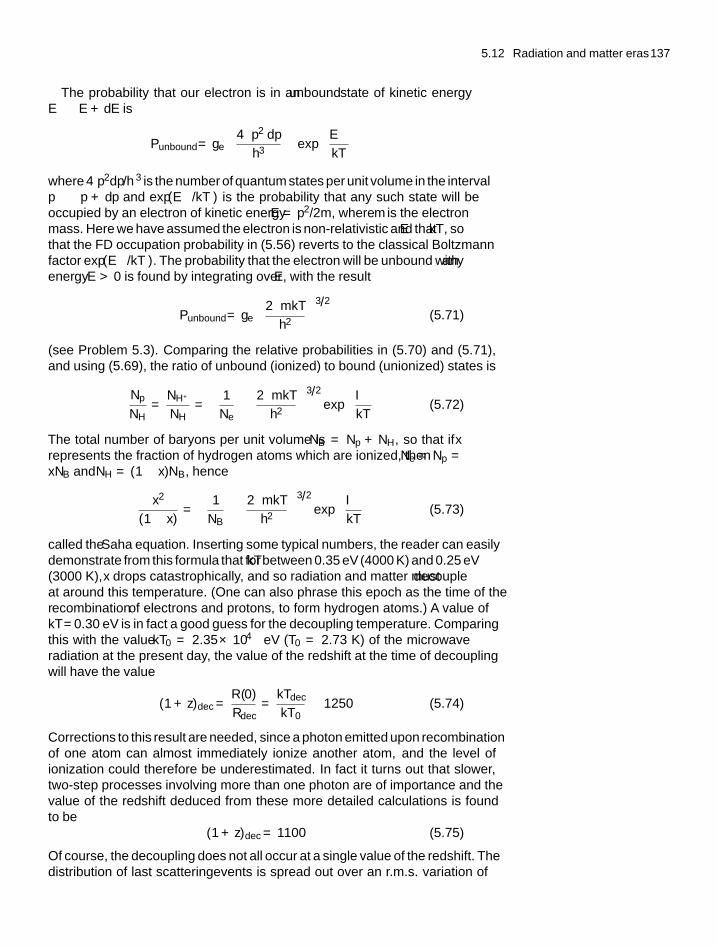
5.12 Radiation and matter eras 137
The probability that our electron is in an unbound state of kinetic energyE → E + dE is
Punbound = ge
(4πp2 dp
h3
)exp
(−E
kT
)where 4πp2dp/h3 is the number of quantum states per unit volume in the intervalp → p + dp and exp (−E/kT ) is the probability that any such state will beoccupied by an electron of kinetic energy E = p2/2m, where m is the electronmass. Here we have assumed the electron is non-relativistic and that E � kT , sothat the FD occupation probability in (5.56) reverts to the classical Boltzmannfactor exp (−E/kT ). The probability that the electron will be unbound with anyenergy E > 0 is found by integrating over E, with the result
Punbound = ge
(2πmkT
h2
)3/2
(5.71)
(see Problem 5.3). Comparing the relative probabilities in (5.70) and (5.71),and using (5.69), the ratio of unbound (ionized) to bound (unionized) states is
Np
NH= NH+
NH=(
1
Ne
)(2πmkT
h2
)3/2
exp
(−I
kT
)(5.72)
The total number of baryons per unit volume is NB = Np + NH, so that if xrepresents the fraction of hydrogen atoms which are ionized, then Ne = Np =xNB and NH = (1 − x)NB, hence
x2
(1 − x)=(
1
NB
)(2πmkT
h2
)3/2
exp
(−I
kT
)(5.73)
called the Saha equation. Inserting some typical numbers, the reader can easilydemonstrate from this formula that for kT between 0.35 eV (4000 K) and 0.25 eV(3000 K), x drops catastrophically, and so radiation and matter must decoupleat around this temperature. (One can also phrase this epoch as the time of therecombination of electrons and protons, to form hydrogen atoms.) A value ofkT = 0.30 eV is in fact a good guess for the decoupling temperature. Comparingthis with the value kT0 = 2.35 × 10⁻⁴ eV (T0 = 2.73 K) of the microwaveradiation at the present day, the value of the redshift at the time of decouplingwill have the value
(1 + z)dec = R(0)
Rdec= kTdec
kT0≈ 1250 (5.74)
Corrections to this result are needed, since a photon emitted upon recombinationof one atom can almost immediately ionize another atom, and the level ofionization could therefore be underestimated. In fact it turns out that slower,two-step processes involving more than one photon are of importance and thevalue of the redshift deduced from these more detailed calculations is foundto be
(1 + z)dec = 1100 (5.75)
Of course, the decoupling does not all occur at a single value of the redshift. Thedistribution of ‘last scattering’events is spread out over an r.m.s. variation of
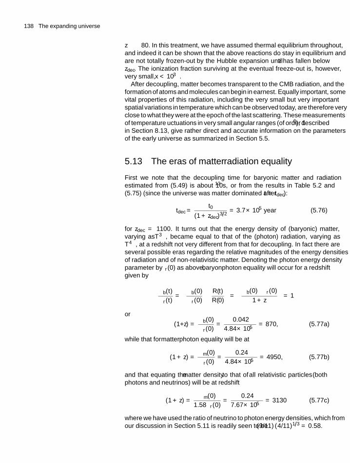
138 The expanding universe
�z ∼ 80. In this treatment, we have assumed thermal equilibrium throughout,and indeed it can be shown that the above reactions do stay in equilibrium andare not totally ‘frozen-out’ by the Hubble expansion until z has fallen belowzdec. The ionization fraction surviving at the eventual freeze-out is, however,very small, x < 10−3.
After decoupling, matter becomes transparent to the CMB radiation, and theformation of atoms and molecules can begin in earnest. Equally important, somevital properties of this radiation, including the very small but very importantspatial variations in temperature which can be observed today, are therefore veryclose to what they were at the ‘epoch of the last scattering’. These measurementsof temperature fluctuations in very small angular ranges (of order 10), describedin Section 8.13, give rather direct and accurate information on the parametersof the early universe as summarized in Section 5.5.
5.13 The eras of matter–radiation equality
First we note that the decoupling time for baryonic matter and radiationestimated from (5.49) is about 1013 s, or from the results in Table 5.2 and(5.75) (since the universe was matter dominated after t = tdec):
tdec = t0
(1 + zdec)3/2
= 3.7 × 10⁵ year (5.76)
for zdec = 1100. It turns out that the energy density of (baryonic) matter,varying as T−3, became equal to that of the (photon) radiation, varying asT−4, at a redshift not very different from that for decoupling. In fact there areseveral possible eras regarding the relative magnitudes of the energy densitiesof radiation and of non-relativistic matter. Denoting the photon energy densityparameter by �r(0) as above, baryon–photon equality will occur for a redshiftgiven by
�b(t)
�r(t)=[�b(0)
�r(0)
] [R(t)
R(0)
]=[
�b(0)/�r(0)
1 + z
]= 1
or
(1+z) = �b(0)
�r(0)= 0.042
4.84 × 10−5= 870, (5.77a)
while that for matter–photon equality will be at
(1 + z) = �m(0)
�r(0)= 0.24
4.84 × 10−5= 4950, (5.77b)
and that equating the matter density to that of all relativistic particles (bothphotons and neutrinos) will be at redshift
(1 + z) = �m(0)
1.58�r(0)= 0.24
7.67 × 10−5= 3130 (5.77c)
where we have used the ratio of neutrino to photon energy densities, which fromour discussion in Section 5.11 is readily seen to be (9/11) (4/11)1/3 = 0.58.
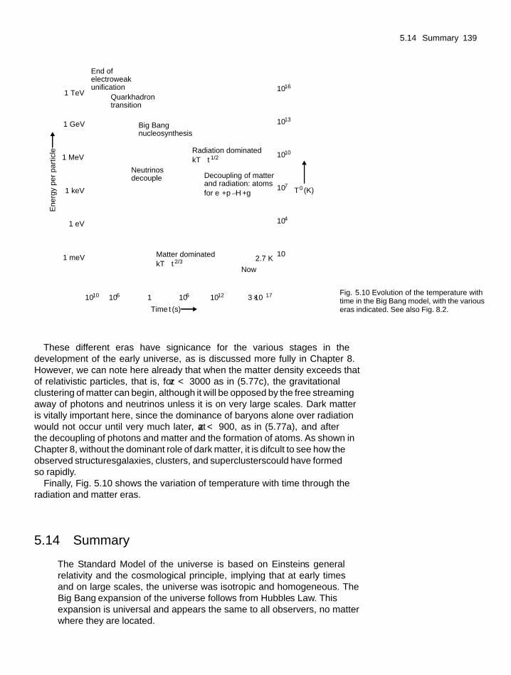
5.14 Summary 139
End ofelectroweakunification
Quark–hadrontransition
Big Bangnucleosynthesis
Neutrinosdecouple
Now
2.7 KMatter dominatedkT ∝ t –2/3
Radiation dominatedkT ∝ t –1/2
10–10 10–6 1 106 1012
10
104
107
1010
1013
1016
3 × 10¹⁷
Time t (s)
T 0 (K)
1 TeV
1 GeV
1 MeV
1 keV
1 meV
1 eV
Ene
rgy
per
part
icle
Decoupling of matterand radiation: atomsfor e– +p H +g
Fig. 5.10 Evolution of the temperature withtime in the Big Bang model, with the variouseras indicated. See also Fig. 8.2.
These different eras have significance for the various stages in thedevelopment of the early universe, as is discussed more fully in Chapter 8.However, we can note here already that when the matter density exceeds thatof relativistic particles, that is, for z < 3000 as in (5.77c), the gravitationalclustering of matter can begin, although it will be opposed by the free streamingaway of photons and neutrinos unless it is on very large scales. Dark matteris vitally important here, since the dominance of baryons alone over radiationwould not occur until very much later, at z < 900, as in (5.77a), and afterthe decoupling of photons and matter and the formation of atoms. As shown inChapter 8, without the dominant role of dark matter, it is difficult to see how theobserved structures—galaxies, clusters, and superclusters—could have formedso rapidly.
Finally, Fig. 5.10 shows the variation of temperature with time through theradiation and matter eras.
5.14 Summary
• The ‘Standard Model’ of the universe is based on Einstein’s generalrelativity and the cosmological principle, implying that at early timesand on large scales, the universe was isotropic and homogeneous. The‘Big Bang’ expansion of the universe follows from Hubble’s Law. Thisexpansion is universal and appears the same to all observers, no matterwhere they are located.
140 The expanding universe
• Hubble’s Law describes the linear relation between the redshift z of thelight from distant galaxies and the universal expansion parameter R, withR0/Re = λobserved/λemitted = (1 + z).
• The Friedmann equation relates the Hubble expansion parameterH = R/R to the total energy density of the universe and the curvature ofspace (the parameter k).
• The total energy density is the sum of contributions from matter, radiation,and vacuum energy (or so-called dark energy). The vacuum term playsthe role of Einstein’s cosmological constant.
• The age of the universe is about 14 Gyr. Independent estimates, fromradioactive isotope ratios, from stellar population analysis, and fromthe most recently measured cosmological parameters (�m = 0.26,�� = 0.74) are all in agreement on the age. The radius of the observableuniverse, that is, the distance to the present optical horizon, is about14 Gpc.
• The curvature parameter of the universe, as measured in experimentsto be described in Chapter 8, is k ≈ 0. On largeer scales, the universeis flat, and its total energy—mass energy, kinetic energy, and potentialenergy—is near to zero.
• The all-pervading and isotropic microwave background radiation has ablack body spectrum of T = 2.725 K and is the cooled remnant of theHot Big Bang.
• The baryonic matter and (photonic) radiation energy densities were equalat redshift z ∼ 103, when the universe was about 400,000 years old.Around that time, radiation and matter decoupled, and atoms (mainlyhydrogen) started to form because of the recombination of electrons andprotons.
• The total matter energy density (including dark matter) started to exceedthat of all radiation (both photons and relativistic neutrinos) below asomewhat larger (and earlier) redshift of z ∼ 3000, and this was animportant factor in the early gravitational clustering of matter on thelargest scales.
Problems
For all constants required refer to Appendix A. More challengingproblems are marked by an asterisk.
(5.1) Assuming that the age of the universe is 14 Gyr andthat the total density is equal to the critical densityρc = 9 × 10⁻²⁷ kg m−3, estimate the gravitationalbinding energy and compare it with the total massenergy of the universe.
(5.2) Calculate the (non-relativistic) escape velocity v of aparticle from the surface of a sphere of radius r anduniform mass density ρ. Show that if one assumes
Hubble’s Law v = Hr, the particle will escape providedthat ρ < 3H 2/8πG.
(5.3) Free non-relativistic fermions of rest-mass m inthermal equilibrium at temperature T are describedby the FD distribution (5.56). If kT mc2,show that the number density of particles is
g(2πmkT/h2
)3/2exp(−mc2/kT
)where g is the
number of spin substates.
(5.4) It is estimated that dark vacuum energy todaycontributes approximately 0.75 to the closure
Problems 141
parameter �. At what value of the redshift parameterand at what age of the universe would vacuum energyhave been less than 10−4 of the energy density ofradiation?
(5.5) The total amount of energy incident on the Earth’satmosphere from the Sun is 0.135 Joules per cm2 persecond (the solar constant). The Earth–Sun distance isD = 1.5 × 10¹¹ m and the solar radius is RS = 7 × 10⁸
m. Assuming that the Sun is a black body, calculate itssurface temperature.
(5.6) It was once proposed that the expansion of the universecould be attributed to an electrostatic repulsionbetween atoms, on the grounds that the arithmeticvalues of the electric charges of the electron and theproton might have a very small fractional differenceε. What value of ε would have been necessary?(Note: This hypothesis was quickly disproved byexperiment, showing that ε was less than 1% of thevalue required. See proposal by Bondi and Littleton(1959) and experimental disproof by Cranshaw andHillas (1959).
*(5.7) Find expressions for the dependence of the time t onthe density ρ for an expanding ‘flat’ universe (k = 0)dominated (a) by radiation and (b) by non-relativisticconserved matter. Show that, in either case, t isof the same order of magnitude as the time for thegravitational free-fall collapse of a body of density ρ
from rest.
*(5.8) In a flat matter-dominated universe (k = 0) of age t0,light from a certain galaxy exhibits a redshift z = 0.95.How long has it taken the light signal to reach us fromthis galaxy? (For a hint, consult equation (8.1)).
(5.9) What is the minimum value of �� which will result inan expansion for the case of a flat universe? Neglectthe contribution to the energy density from radiation.
(5.10) Prove the statement that the gravitational fieldanywhere inside a spherical shell of uniform density iszero; and that the field outside a spherical distributionof total mass M is equal to that of a point mass M placedat the centre of the sphere (This is called Newton’s Lawof Spheres in classical mechanics. In general relativityit is known as Birkhoff’s theorem.)
*(5.11) Derive a formula for the age of an open universe (� <
1) with zero cosmological constant and negligibleradiation density. Use Equation (5.39) and Example5.3 as a guide. Calculate the age for � = 0.24. (Hint:Make the substitution tan2 θ = (1 + z)�/(1 − �).
*(5.12) Show that, as indicated above, the temperature belowwhich neutrinos decouple from other matter andradiation in the early, radiation-dominated universe, iskT ∼3 MeV. Hints for the stages in solving this problemare as follows:
(1) Start with the cross-section for the process e+ +e− → ve + ve, via W -exchange, which is givenin Example 3.2 as σ = G2
Fs/(6π), where s is theCMS energy squared and it is assumed that massescan be neglected (i.e.
√s � mec2). Evaluate this
cross-section in cm2 when s is in MeV2.(2) Show that, treating the electrons and positrons as a
Fermi gas of relativistic particles the mean valueof s at temperature T is given by 〈s〉 = 2〈E〉2
where 〈E〉 is the mean energy of the particles inthe distribution, which can be found from equation(5.56).
(3) Calculate the density Ne of electrons and positronsas a function of kT, and hence the rate for the abovereaction, W = 〈σv〉Ne where v is the relativevelocity of the particles, as a function of kT.
(4) Using (5.49) and (5.58) calculate the time t ofthe expansion as a function of kT, and setting thisequal to 1/W , deduce the value of kT at neutrinodecoupling.
6 Nucleosynthesis andbaryogenesis
6.1 Primordial nucleosynthesis
In continuation of this discussion of the early universe, we next turn our attentionto the synthesis of the nuclei of the light elements—4He, 2H, 3He, and 7Li. Theagreement between the predicted and measured abundances of these elementsprovided early support for the Big Bang hypothesis.
As discussed in Section 5.10, once the universe had cooled to a temperaturekT < 100 MeV, or after a time t > 10−4 s, essentially all the hadrons, withthe sole exception of neutrons and protons and their antiparticles, would havedisappeared by decay. The nucleons and antinucleons would have been presentin equal numbers and have nearly, but not quite completely, annihilated toradiation. As described in the next section, once the temperature had fallenbelow kT = 20 MeV, a tiny residue of about one billionth of the originalnumbers of protons and neutrons must have survived to form the stuff of thematerial universe we inhabit today. The relative numbers of these survivingprotons and neutrons would have been determined by the weak reactions
ve + n ↔ e− + p (6.1)
ve + p ↔ e+ + n (6.2)
n → p + e− + ve (6.3)
Since at the temperatures considered, the nucleons are non-relativistic, then justas in the analysis of Section 5.12, the equilibrium ratio of neutrons to protonswill be governed by the ratio of the Boltzmann factors, so that
Nn
Np= exp
(−Q
kT
); Q = (Mn − Mp
)c2 = 1.293 MeV (6.4)
The rate or width � for the first two reactions (6.1) and (6.2) must vary as T 5
purely on dimensional grounds. The Fermi constant GF from (1.9) or Table1.5 has dimensions E−2, so the cross-section σ (dimension E−2) must varyas G2
FT 2 and the incident flux φ, proportional to the neutrino density, as T 3.Hence the width � = σφ gets a T 5 factor. On the other hand the expansionrate of the radiation-dominated universe is H ∼ g∗1/2
T 2 from (5.59). Hence�/H ∼ T 3/(g∗)1/2 and as the universe expands and the temperature falls, theabove reactions will go out of equilibrium when W/H < 1, where W = �/h.In fact, as described in Chapter 5, at kT < 3 MeV neutrinos are already goingout of equilibrium with electrons in the process e+ + e− ↔ v + v, since thishas an even smaller cross-section than (6.2) because of the smaller target mass.
6.1 Primordial nucleosynthesis 143
Inserting typical values for the cross-sections for (6.1) and (6.2), the neutrinodensity (5.57) and the Hubble parameter (5.59), it is easy to demonstrate thatthe freeze-out temperature will be of order 1 MeV—see Problem 6.2. In factthe result of a full calculation for the above reactions gives for the freeze-outa value kT = 0.80 MeV, so that the initial value of the neutron–proton ratiowill be
Nn (0)
Np (0)= exp
(−Q
kT
)= 0.20 (6.5)
After some time, neutrons will disappear by decay in reaction (6.3). Attime t after decoupling, there will then be Nn(0) exp(−t/τ) neutrons and[Np(0) + Nn(0){1 − exp(−t/τ)}] protons, with a neutron–proton ratio of
Nn (t)
Np (t)= 0.20 exp (−t/τ)
[1.20 − 0.20 exp (−t/τ)](6.6)
where τ = 885.7 ± 0.8 s is the presently quoted value of the free neutronlifetime. If nothing else were to happen at this juncture, the neutrons wouldsimply die away by decay and the early universe would consist exclusively ofprotons and electrons. However, as soon as neutrons appear, nucleosynthesiscan begin in a first stage, with the formation of deuterons:
n + p ↔ 2H + γ + Q (6.7)
where the deuteron binding energy Q = 2.22 MeV. This is an electromagneticprocess with a cross-section of 0.1 mb, very much larger than those of theweak processes (6.1)–(6.3), and consequently it stays in thermal equilibriumfor very much longer. As indicated below, there is at this time a billion-foldpreponderance of photons over nucleons, and the deuterons are not frozen-out until the temperature falls to about Q/40, that is, kT = 0.05 − 0.06 MeV(see Problem 6.3). As soon as the reverse process of photodisintegration ofthe deuteron ceases, competing reactions in a second stage leading to heliumproduction take over, for example,
2H + n → 3H + γ
2H + H → 3He + γ
2H + 2H → 4He + γ
3H + 2H → 4He + n
3H + p → 4He + γ
which then lead in a third stage to lithium and beryllium production:
3He + 4He → 7Be + γ
7Be + n → 7Li + p
For kT = 0.05 MeV, corresponding to an expansion time from (5.49) of t ∼300 s for Nν = 3, the neutron–proton ratio from (6.6) becomes
r = Nn
Np= 0.135 (6.8)
144 Nucleosynthesis and baryogenesis
The expected helium mass fraction, with the mass of the helium nucleus setequal to 4 times that of the proton is then given by
Y = 4NHe
(4NHe + NH)= 2r
(1 + r)≈ 0.24 (6.9)
The mass fraction Y has been measured in a variety of celestial sites, includingstellar atmospheres, planetary nebulae, globular clusters, gas clouds, and so on,with values in the range
Y = 0.238 ± 0.006 (6.10)
Problems in evaluating both the predicted and measured values mean thatagreement between theory (6.9) and observation (6.10) is still uncertain at the5% level. Nevertheless, this level of agreement was an early and very importantsuccess for the Big Bang model. It should be pointed out here that the observedhelium mass fraction is far greater than that which could have been producedin hydrogen burning in main sequence stars; their contribution adds only 0.01to the ratio Y (see Problem 6.4).
An important feature of nucleosynthesis in the Big Bang scenario is thatit accounts not only for 4He but also for the light elements D, 3He, and 7Li,which occur in small but significant amounts, far more in fact than would havesurvived if they had only been produced in thermonuclear interactions in stellarinteriors. The lithium and deuterium abundances give
Li
H= (1.23 ± 0.01) × 10−10 (6.11)
D
H= (2.6 ± 0.4) × 10−5 (6.12)
The curves in Fig. 6.1 shows the abundances expected from primordialnucleosynthesis, calculated on the basis of the cross-sections involved, andplotted in terms of the (present day) baryon to photon density ratio. The result(6.12) on the deuterium–hydrogen ratio leads to a value of the baryon densityin the range
ρB = (4.0 ± 0.4) × 10−28 kg m−3 (6.13)
and a contribution to the closure parameter
�B = 0.044 ± 0.005 (6.14)
corresponding to a number density of baryons NB = 0.24 ± 0.03 m−3.Comparing with the number density of microwave photons (5.52), this yieldsfor the baryon–photon ratio
NB
Nγ
≈(NB − NB
)Nγ
= (6.1 ± 0.6) × 10−10 (6.15)
A slightly different value of (6.5 ± 0.4) × 10−10 is found from the analysisof microwave anisotropies by the WMAP (Wilkinson Microwave AnisotropyProbe), described in Chapter 8. This value for the baryon–photon ratio wouldimply for the helium fraction, Y = 0.248, about 5% larger than the observedvalue in (6.10).
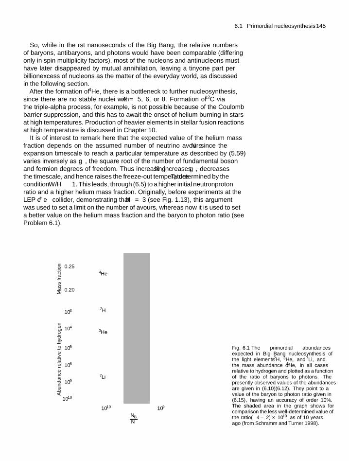
6.1 Primordial nucleosynthesis 145
So, while in the first nanoseconds of the Big Bang, the relative numbersof baryons, antibaryons, and photons would have been comparable (differingonly in spin multiplicity factors), most of the nucleons and antinucleons musthave later disappeared by mutual annihilation, leaving a tiny—one part perbillion—excess of nucleons as the matter of the everyday world, as discussedin the following section.
After the formation of 4He, there is a bottleneck to further nucleosynthesis,since there are no stable nuclei with A = 5, 6, or 8. Formation of 12C viathe triple-alpha process, for example, is not possible because of the Coulombbarrier suppression, and this has to await the onset of helium burning in starsat high temperatures. Production of heavier elements in stellar fusion reactionsat high temperature is discussed in Chapter 10.
It is of interest to remark here that the expected value of the helium massfraction depends on the assumed number of neutrino flavours Nν since theexpansion timescale to reach a particular temperature as described by (5.59)varies inversely as
√g∗, the square root of the number of fundamental boson
and fermion degrees of freedom. Thus increasing Nν increases g∗, decreasesthe timescale, and hence raises the freeze-out temperature TF determined by thecondition W/H ∼ 1. This leads, through (6.5) to a higher initial neutron–protonratio and a higher helium mass fraction. Originally, before experiments at theLEP e+e− collider, demonstrating that Nν = 3 (see Fig. 1.13), this argumentwas used to set a limit on the number of flavours, whereas now it is used to seta better value on the helium mass fraction and the baryon to photon ratio (seeProblem 6.1).
10–10
10–10 10–9
10–9
10–6
10–5
10–4
10–3
0.20
0.25
Abu
ndan
ce r
elat
ive
to h
ydro
gen
Mas
s fr
actio
n
7Li
3He
2H
4He
� ≡NBNγ
Fig. 6.1 The primordial abundancesexpected in Big Bang nucleosynthesis ofthe light elements 2H, 3He, and 7Li, andthe mass abundance of 4He, in all casesrelative to hydrogen and plotted as a functionof the ratio of baryons to photons. Thepresently observed values of the abundancesare given in (6.10)–(6.12). They point to avalue of the baryon to photon ratio given in(6.15), having an accuracy of order 10%.The shaded area in the graph shows forcomparison the less well-determined value ofthe ratio—(4 ± 2) × 10−10—as of 10 yearsago (from Schramm and Turner 1998).
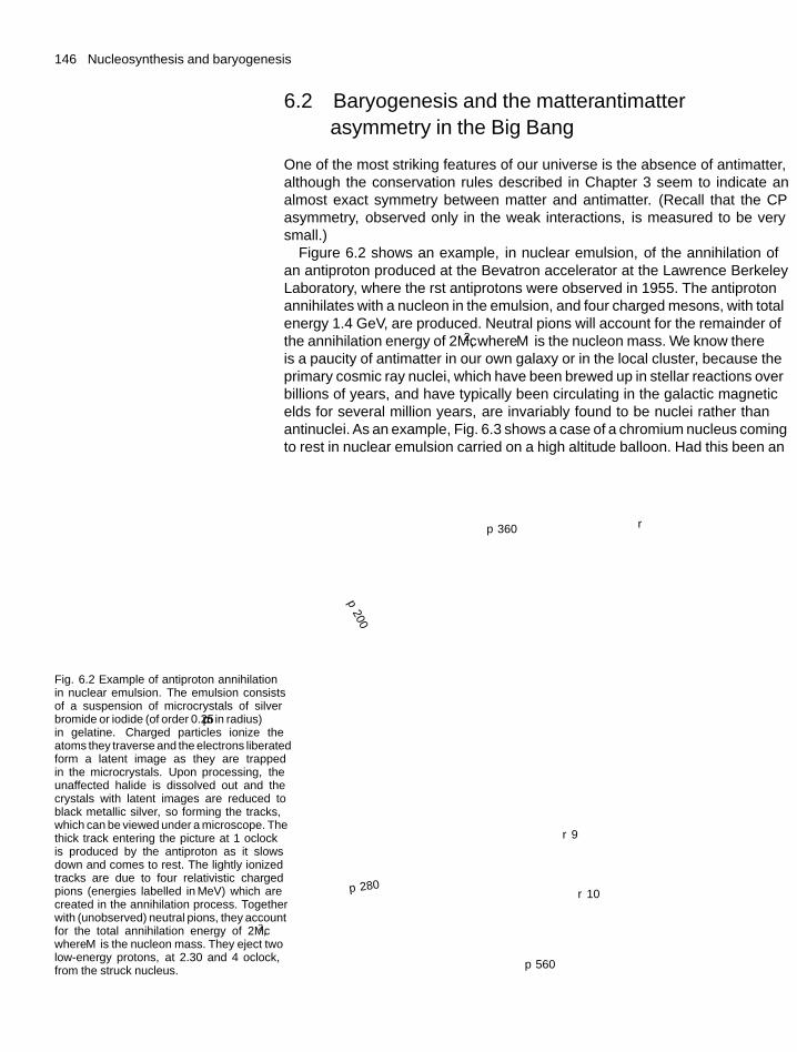
146 Nucleosynthesis and baryogenesis
6.2 Baryogenesis and the matter–antimatterasymmetry in the Big Bang
One of the most striking features of our universe is the absence of antimatter,although the conservation rules described in Chapter 3 seem to indicate analmost exact symmetry between matter and antimatter. (Recall that the CPasymmetry, observed only in the weak interactions, is measured to be verysmall.)
Figure 6.2 shows an example, in nuclear emulsion, of the annihilation ofan antiproton produced at the Bevatron accelerator at the Lawrence BerkeleyLaboratory, where the first antiprotons were observed in 1955. The antiprotonannihilates with a nucleon in the emulsion, and four charged mesons, with totalenergy 1.4 GeV, are produced. Neutral pions will account for the remainder ofthe annihilation energy of 2Mc2, where M is the nucleon mass. We know thereis a paucity of antimatter in our own galaxy or in the local cluster, because theprimary cosmic ray nuclei, which have been brewed up in stellar reactions overbillions of years, and have typically been circulating in the galactic magneticfields for several million years, are invariably found to be nuclei rather thanantinuclei. As an example, Fig. 6.3 shows a case of a chromium nucleus comingto rest in nuclear emulsion carried on a high altitude balloon. Had this been an
Fig. 6.2 Example of antiproton annihilationin nuclear emulsion. The emulsion consistsof a suspension of microcrystals of silverbromide or iodide (of order 0.25μm in radius)in gelatine. Charged particles ionize theatoms they traverse and the electrons liberatedform a latent image as they are trappedin the microcrystals. Upon processing, theunaffected halide is dissolved out and thecrystals with latent images are reduced toblack metallic silver, so forming the tracks,which can be viewed under a microscope. Thethick track entering the picture at 1 o’clockis produced by the antiproton as it slowsdown and comes to rest. The lightly ionizedtracks are due to four relativistic chargedpions (energies labelled in MeV) which arecreated in the annihilation process. Togetherwith (unobserved) neutral pions, they accountfor the total annihilation energy of 2Mc2,where M is the nucleon mass. They eject twolow-energy protons, at 2.30 and 4 o’clock,from the struck nucleus.
p 360
p200
r–
r 9
r 10
p 560
p 280
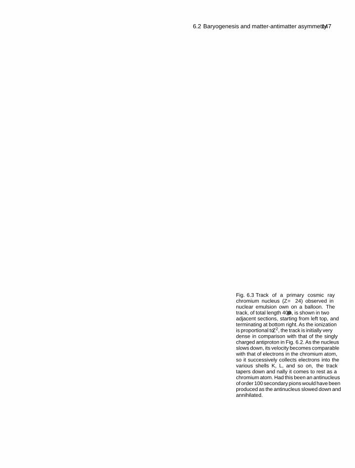
6.2 Baryogenesis and matter-antimatter asymmetry 147
Fig. 6.3 Track of a primary cosmic raychromium nucleus (Z = 24) observed innuclear emulsion flown on a balloon. Thetrack, of total length 400μm, is shown in twoadjacent sections, starting from left top, andterminating at bottom right. As the ionizationis proportional to Z2, the track is initially verydense in comparison with that of the singlycharged antiproton in Fig. 6.2. As the nucleusslows down, its velocity becomes comparablewith that of electrons in the chromium atom,so it successively collects electrons into thevarious shells K, L, and so on, the tracktapers down and finally it comes to rest as achromium atom. Had this been an antinucleusof order 100 secondary pions would have beenproduced as the antinucleus slowed down andannihilated.
148 Nucleosynthesis and baryogenesis
antinucleus, the subsequent annihilation would have been 24 times as violentas that in Fig. 6.2.
On a wider scale, there is absolutely no evidence for the intense γ-ray andX-ray emission which would follow annihilation of matter in distant galaxieswith clouds of antimatter. The results of nucleon–antinucleon annihilation afterrecombination of hydrogen atoms at z ∼ 1100 would also have had significanteffects on the Planck black body distribution of the cosmic microwavespectrum. Very low fluxes of positrons and antiprotons do exist in thecosmic rays incident on the Earth’s atmosphere, but these can be accountedfor in terms of the processes of electron–positron or proton–antiprotonpair creation resulting from collisions of high-energy γ-rays or nuclei withinterstellar matter.
While it is true that in all laboratory experiments to date, baryon numberis conserved, there are in fact no compelling theoretical reasons why thisshould be so, especially since the early universe would have involved very hightemperatures and energies and possibly new types of particles and interactions,which are out of reach at laboratory energies. Indeed, the history of particlephysics contains several long-respected conservation laws, which have finallyfallen by the wayside, as already described in Chapter 3.
The electric charge, we know, is strictly conserved in all situations,because it is protected by gauge invariance and the existence of a long-rangeelectromagnetic field coupled to the electric charge. An absolute conservationlaw for baryons ought to have as a consequence the existence of a new long-range field coupled to baryon number. There is no evidence for any such field.If we assume the validity of the equivalence principle described in Chapter 2,the results of the torsion balance experiments in Section 2.3 allow one to setlimits for any such field, as follows.
Two bodies of different materials but the same mass will have slightlydifferent baryon numbers—typically by 0.1%—because of variations in bindingenergy per nucleon with the mass number A, and because of the neutron–protonmass difference and variations with A of the neutron–proton ratio (see Fig. 10.1).So, assuming the validity of the equivalence principle, these experiments findno evidence of any such new long-range field coupled to baryon number andset a limit for such a coupling of less than 10−9G where G is the Newtonianconstant. These statements also apply to lepton number conservation—again,there are no compelling theoretical reasons for it.
6.3 The baryon–photon ratio in the Big Bang
What predictions does the Big Bang model make for the baryon/antibaryon andthe baryon/photon ratios, if we assume strict conservation of baryon number?In the early stages of the Big Bang, when the thermal energy per particle kT(where k is Boltzmann’s constant) was large compared with the hadron masses,it is expected that many types of hadrons, including protons and neutrons andtheir antiparticles, would have been in thermal equilibrium with radiation, beingcreated and annihilated in reversible reactions such as
p + p ↔ γ + γ (6.16)
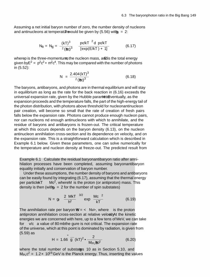
6.3 The baryon–photon ratio in the Big Bang 149
Assuming a net initial baryon number of zero, the number density of nucleonsand antinucleons at temperature T would be given by (5.56) with gf = 2:
NB = NB = (kT )3
π2 (hc)3
∫ (pc/kT
)2d(pc/kT
)[exp (E/kT ) + 1]
(6.17)
where p is the three-momentum, m the nucleon mass, and E is the total energygiven by E2 = p2c2 +m2c4. This may be compared with the number of photonsin (5.52):
Nγ = 2.404 (kT )3
π2 (hc)3(6.18)
The baryons, antibaryons, and photons are in thermal equilibrium and will stayin equilibrium as long as the rate for the back reaction in (6.16) exceeds theuniversal expansion rate, given by the Hubble parameter H . Eventually, as theexpansion proceeds and the temperature falls, the part of the high-energy tail ofthe photon distribution, with photons above threshold for nucleon–antinucleonpair creation, will become so small that the rate of creation of fresh pairsfalls below the expansion rate. Photons cannot produce enough nucleon pairs,nor can nucleons find enough antinucleons with which to annihilate, and theresidue of baryons and antibaryons is ‘frozen-out’. The critical temperatureat which this occurs depends on the baryon density (6.13), on the nucleon–antinucleon annihilation cross-section and its dependence on velocity, and onthe expansion rate. This is a straightforward calculation which is described inExample 6.1 below. Given these parameters, one can solve numerically forthe temperature and nucleon density at freeze-out. The predicted result from
Example 6.1 Calculate the residual baryon–antibaryon ratio after anni-hilation processes have been completed, assuming baryon–antibaryonequality initially and conservation of baryon number.
Under these assumptions, the number density of baryons and antibaryonscan be easily found by integrating (6.17), assuming that the thermal energyper particle kT Mc2, where M is the proton (or antiproton) mass. Thisdensity is then (with gf = 2 for the number of spin substates)
N = gf
(2πMkT
h2
)3/2
exp
(−Mc2
kT
)(6.19)
The annihilation rate per baryon is W = <σNv>, where σ is the proton–antiproton annihilation cross-section at relative velocity v. At the kineticenergies we are concerned with here, up to a few tens of MeV, we can takefor 〈σv/c〉 a value of 80 mb—the figure is not critical. The expansion rateof the universe, which at this point is dominated by radiation, is given from(5.59) as
H = 1.66√
g∗ (kT )2 · 2π(MPLhc2
) (6.20)
where the total number of substates g∗ ∼ 10 as in Section 5.10, andMPLc2 = 1.2 × 10¹⁹ GeV is the Planck energy. Thus, inserting the values
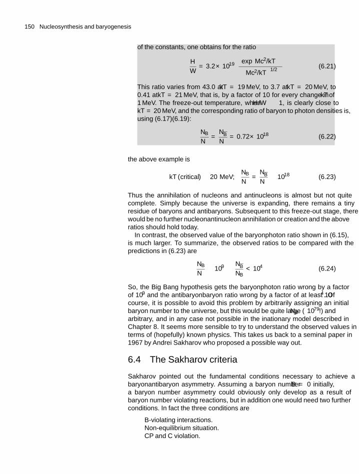
150 Nucleosynthesis and baryogenesis
of the constants, one obtains for the ratio
H
W= 3.2 × 10⁻¹⁹
[exp(Mc2/kT
)][Mc2/kT
]1/2(6.21)
This ratio varies from 43.0 at kT = 19 MeV, to 3.7 at kT = 20 MeV, to0.41 at kT = 21 MeV, that is, by a factor of 10 for every change in kT of1 MeV. The freeze-out temperature, when H/W ∼ 1, is clearly close tokT = 20 MeV, and the corresponding ratio of baryon to photon densities is,using (6.17)–(6.19):
NB
Nγ
= NB
Nγ
= 0.72 × 10⁻¹⁸ (6.22)
the above example is
kT (critical) ≈ 20 MeV;NB
Nγ
= NB
Nγ
∼ 10−18 (6.23)
Thus the annihilation of nucleons and antinucleons is almost but not quitecomplete. Simply because the universe is expanding, there remains a tinyresidue of baryons and antibaryons. Subsequent to this freeze-out stage, therewould be no further nucleon–antinucleon annihilation or creation and the aboveratios should hold today.
In contrast, the observed value of the baryon–photon ratio shown in (6.15),is much larger. To summarize, the observed ratios to be compared with thepredictions in (6.23) are
NB
Nγ
≈ 10−9 NB
NB< 10−4 (6.24)
So, the Big Bang hypothesis gets the baryon–photon ratio wrong by a factorof 109 and the antibaryon–baryon ratio wrong by a factor of at least 104. Ofcourse, it is possible to avoid this problem by arbitrarily assigning an initialbaryon number to the universe, but this would be quite large (NB ∼ 1079!) andarbitrary, and in any case not possible in the inflationary model described inChapter 8. It seems more sensible to try to understand the observed values interms of (hopefully) known physics. This takes us back to a seminal paper in1967 by Andrei Sakharov who proposed a possible way out.
6.4 The Sakharov criteria
Sakharov pointed out the fundamental conditions necessary to achieve abaryon–antibaryon asymmetry. Assuming a baryon number B = 0 initially,a baryon number asymmetry could obviously only develop as a result ofbaryon number violating reactions, but in addition one would need two furtherconditions. In fact the three conditions are
• B-violating interactions.• Non-equilibrium situation.• CP and C violation.
6.5 The baryon–antibaryon asymmetry: possible scenarios 151
The first requirement is obvious and its possibility has been discussed inconnection with the grand unified theory (GUT) models and the search forproton decay in Section 4.3. At present, there is no direct laboratory evidencethat baryon number is violated, so we just retain it as an assumption. Thesecond condition follows from the fact that, in thermal equilibrium, the particledensity depends only on the particle mass and the temperature. Since particleand antiparticle have identical masses by the CPT theorem (see Section 3.14),no asymmetry could develop. Put another way, at equilibrium, any reactionwhich destroys baryon number will be exactly counterbalanced by the inversereaction which creates it. Third, as pointed out in Chapter 3, C and CP violationare necessary if antimatter is to be distinguished unambiguously from matteron a cosmic scale. We now discuss models for which these conditions canhopefully be met.
6.5 The baryon–antibaryon asymmetry: possiblescenarios
The precise mechanism responsible for generating a baryon–antibaryonasymmetry of the observed magnitude is presently unknown, although severalmodels have been suggested over the last two or three decades. Three of thepossibilities are
• GUT baryogenesis.• Electroweak baryogenesis.• Baryogenesis via leptogenesis.
6.5.1 Baryogenesis in the SU(5) GUT model
We first consider baryon number violation via the SU(5) model of grandunification. In that model, already discussed in Chapter 4, quarks and leptons areincorporated in the same multiplets, and quark–lepton transitions can thereforetake place, with the interesting possibility of proton decay. Indeed this wasone of the predictions in Sakharov’s 1967 paper. However, he assumed themediating bosons of the unified theory had masses of order the Planck mass,resulting in prediction of an unobservably long lifetime of 1050 years. Forexample, as shown in Section 4.3, in the SU(5) model a proton can transforminto a pion and a positron via virtual X -boson exchange. In this transition, boththe baryon number B and the lepton number L have decreased by one unit, sothat the difference (B−L) is conserved, while (B+L) is violated. This turns outto be a crucial feature in the discussion of possible mechanisms for generatingbaryon asymmetry.
The mediating ‘leptoquark’ bosons X , Y , and their antiparticles of the GUTsymmetry are supposedly created in the Big Bang on a 10−40 s timescale, andare expected to decay out of thermal equilibrium. The requirements are for twodecay channels, say 1 and 2, of different baryon number. Suppose that x and(1−x) are the branching ratios for decay of X to modes with baryon number B1
and B2 respectively. For the antiparticle X , let the ratios be x and (1 − x), withbaryon numbers −B1 and −B2. Since the numbers of X and X particles areequal, by the CPT theorem, discussed in Chapter 3, the net baryon asymmetry
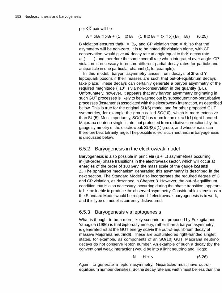
152 Nucleosynthesis and baryogenesis
per X X pair will be
A = xB1 − xB1 + (1 − x) B2 − (1 − x) B2 = (x − x) (B1 − B2) (6.25)
B violation ensures that B1 �= B2, and CP violation that x �= x, so that theasymmetry will be non-zero. It is to be noted that C violation alone, with CPconservation, would give an X decay rate at angle θ equal to the X decay rateat (π − θ), and therefore the same overall rate when integrated over angle. CPviolation is necessary to ensure different partial decay rates for particle andantiparticle in one particular channel (1, for example).
In this model, baryon asymmetry arises from decays of the X and Y‘leptoquark’ bosons if their masses are such that out-of-equilibrium decaystake place. These decays can certainly generate a baryon asymmetry of therequired magnitude (∼ 10−9) via non-conservation in the quantity (B + L).Unfortunately, however, it appears that any baryon asymmetry originating insuch GUT processes is likely to be washed out by subsequent non-perturbativeprocesses (instantons) associated with the electroweak interaction, as describedbelow. This is true for the original SU(5) model and for other proposed GUTsymmetries, for example the group called SO(10), which is more extensivethan SU(5). Most importantly, SO(10) has room for an extra U(1) right-handedMajorana neutrino singlet state, not protected from radiative corrections by thegauge symmetry of the electroweak SU(2) × U(1) group, and whose mass cantherefore be arbitrarily large. The possible role of such neutrinos in baryogenesisis discussed below.
6.5.2 Baryogenesis in the electroweak model
Baryogenesis is also possible in principle via (B + L) asymmetries occurringin (first-order) phase transitions in the electroweak sector, which will occur atenergies of the order of 100 GeV, the mass scale of the gauge bosons W andZ . The sphaleron mechanism generating this asymmetry is described in thenext section. The Standard Model also incorporates the required degree of Cand CP violation, as described in Chapter 3. However, the out-of-equilibriumcondition that is also necessary, occurring during the phase transition, appearsto be too feeble to produce the observed asymmetry. Considerable extensions tothe Standard Model would be required if electroweak baryogenesis is to work,and this type of model is currently disfavoured.
6.5.3 Baryogenesis via leptogenesis
What is thought to be a more likely scenario, first proposed by Fukugita andYanagida (1986) is that a lepton asymmetry, rather than a baryon asymmetry,is generated first at the GUT energy scale via the out-of-equilibrium decay ofmassive Majorana neutrinos, N . These are postulated as right-handed singletstates, for example, as components of an SO(10) GUT. Majorana neutrinodecays do not conserve lepton number. An example of such a decay (by theconventional weak interaction) would be into a light neutrino and Higgs:
N → H + v (6.26)
Again, to generate a lepton asymmetry, the N particles must have out-of-equilibrium number densities. So the decay rate and width must be less than the
6.5 The baryon–antibaryon asymmetry: possible scenarios 153
Hubble parameter, W = �/h H . This requirement puts constraints on theN mass. Most importantly, however, the resulting lepton asymmetry conservesthe quantity (B − L).
In this model, the lepton asymmetry is subsequently converted into a baryonasymmetry by non-perturbative processes at the lower-energy scale of theelectroweak interactions. Here we dip into the somewhat exotic scenario ofgauge anomalies (i.e. divergent terms in the axial–vector weak currents),instantons and sphalerons. Instantons are examples of single events in fieldtheory. One can think of such events as comparable to the process of radioactivedecay by single alpha particle emission through a potential barrier (discussedin Chapter 10). As we noted in Chapter 3, the vacuum state (i.e. the state oflowest energy) in the electroweak model can be quite complex. Indeed, it turnsout that there is an infinite number of degenerate vacuum states with differenttopologies, that is, different baryon and lepton numbers. Adjacent vacua differin the value of (B + L) by 2Nf where Nf = 3 is the number of quark or leptonflavours, and they are separated by potential barriers with a height of the order ofthe electroweak vacuum expectation value v ∼ 200 GeV. On the other hand, thequantity (B − L) is ‘anomaly-free’ and conserved. It turns out that the changein lepton and baryon numbers between adjacent vacua is �L = �B = 3.At normal energies, such changes can happen only by quantum-mechanicaltunnelling through the barrier between one vacuum state and the next. As firstshown by ‘t Hooft in 1973, such a so-called instanton process is enormouslysuppressed by a factor of order exp(−2π/αw) ∼ 10−86, where αw is the weakcoupling.
However, an important observation by Kuzmin et al. (1985) was to point outthat at high enough temperatures, kT > v, thermal transitions can take place byjumping over the barrier, via a 12-fermion interaction referred to as a sphaleron(the name comes from the Greek for an unstable state: the sphaleron is a saddlepoint in configuration space, which sits on the top of the barrier, and can jumpeither way). Typical �B = �L = 3 transitions would be
(u + u + d) + (c + c + s) + (t + t + b) → e+ + μ+ + τ+
(u + d + d) + (c + s + s) + (t + b + b) → ve + vμ + vτ (6.27)
In these transitions, three quarks and one lepton of each of the Nf = 3generations are involved. The degree of baryon–antibaryon asymmetry thusgenerated—typically of the order of half the magnitude of the original leptonasymmetry—depends on the assumed masses M of the massive Majorananeutrinos N . At the same time, the masses of the light neutrinos, which can beestimated from observations of neutrino oscillations described in Chapter 9, areconnected with the M values via the so-called ‘see-saw’ mechanism discussedin Chapter 4. The crucial point here is that the (B − L) asymmetry generated bythe N particles at the GUT scale is preserved in going through the electroweaktransition. This is in contrast with the GUT-generated baryon asymmetry ofSection 6.5.1, where the (B + L) asymmetry is washed out by the very samesphaleron processes which convert lepton asymmetries to baryon asymmetries.
It is remarkable that the Majorana masses ∼ 1010 − 1013 GeV required tofit the light neutrino masses by the see-saw formula also seem to give leptonasymmetries of the correct magnitude to provide, in turn, baryon asymmetries ofabout the magnitude observed in (6.15). Indeed, one can reverse the argument
154 Nucleosynthesis and baryogenesis
and deduce that from the observed baryon asymmetry (∼ 10−9), the abovemechanism would only work if the light neutrino masses were in the range0.01–0.1 eV/c2, exactly where oscillation experiments place them.
There are, however, some problems with this model. Such massive Majorananeutrinos would have to be created during the ‘reheating’ phase immediatelyfollowing inflation, as discussed in Chapter 8. A difficulty here is that, in orderto produce massive neutrinos, a high reheating temperature is required, and insupersymmetric theories this could result in an overproduction of gravitinos(the massive spin 3/2 fermionic partners of the gravitons). The rapid decay ofthese massive gravitinos would certainly produce hadrons, and unfortunatelythis has the effect of completely changing the parameters in nucleosynthesis,so that the good agreement between predictions and observations described inSection 6.1 would be lost.
One suggestion for avoiding this problem has been to appeal to the decay ofinflatons (the fundamental bosons of the inflation model discussed in Chapter 8)to produce the Majorana particles, ϕ → N +N . Thus, the reheating temperaturefollowing the end of inflation can be kT M and the above difficulty can beavoided (Yanagida 2005).
If one believes that all the difficulties can be circumvented, the leptogenesismodel seems to provide a reasonably self-consistent picture, although the ideaspresented are of course very speculative. We do not even know yet whetherneutrinos are Majorana or Dirac particles, and the necessary CP violatingphases in the massive neutrino sector are completely unknown. However, thelink between the observed small masses of the light neutrinos and the observedbaryon–antibaryon asymmetry of the universe, via massive Majorana neutrinosand the see-saw mechanism, if it can be confirmed, would be one of theoutstanding achievements of particle astrophysics. While the true origin ofthe universal baryon asymmetry is at present unknown, the situation for thefuture looks hopeful, with enormous experimental efforts on measurement ofneutrino masses and mixings, and the hoped-for discovery of the Higgs bosonand of supersymmetry.
6.6 Summary
• The observed abundances of the light elements deuterium (2H), helium(3He and 4He), and lithium (7Li) can be understood by their creationin nucleosynthesis at temperatures kT ∼ 0.1 MeV in the first minutesfollowing the Big Bang. Together with the microwave backgroundradiation and the redshift, the light element abundances provide verystrong support for the Big Bang hypothesis. The baryon density fromthe synthesis of the light elements in the first minutes of the universeaccounts for only a small part of the total matter density: most of thematter is dark matter.
• The observed strong asymmetry between matter and antimatter has to beascribed to special baryon number violating and CP violating interactionsoperating at a very early stage of the Big Bang when the temperature wasvery high.
• There is a realistic prospect that, if heavy Majorana neutrinos exist, thebaryon asymmetry of the universe may be directly connected with the
Problems 155
small observed masses of the light neutrinos via the see-saw mechanism,coupled with non-perturbative interactions on the electroweak scale.
Problems
More challenging problems are shown by an asterisk
*(6.1) Calculate the expected mass ratio of primordial heliumto hydrogen, as in (6.9), but for the case of differentnumbers of neutrino flavours Nν = 3, 4, 5, 6, . . .. Showthat each additional flavour will increase the expectedratio by about 5%. Calculate also the expected mass ratiofor Nν = 3 if the neutron—proton mass difference was1.40 MeV/c2 instead of 1.29 MeV/c2, but the free neutronlifetime was unaffected.
*(6.2) In discussing the neutron/proton equilibrium ratio (6.8)it was stated that the rate or width W for the reactionνe+n → e−+p varied as T 5. Verify this directly, referringback to Section (1.8) to compute the cross-section forthe above reaction as a function of T and using therelevant flux density to compute W from (1.14). Assumethat all particles have kinetic energies kT, such thatmec2 kT Mpc2, that is, treat the nucleons as non-relativistic and essentially stationary, while the leptons
are extreme-relativistic. Comparing with the expansionrate (5.59), estimate the temperature at which the neutronsand protons ‘freeze-out’ of equilibrium.
(6.3) Estimate the value of kT below which, in an expandinguniverse, deuterium will undergo ‘freeze-out’ from thereaction n + p ↔ d + γ + Q, where Q = 2.22 MeVis the binding energy of the deuteron. Proceed by firstderiving an analytic expression for the fraction of cosmicmicrowave photons with E � kT . Assume that thephotodisintegration cross-section is σ = 0.1 mb, and takethe Hubble parameter from (5.59), with g∗ = 10.
(6.4) The Sun has a measured luminosity of 3.9 × 1026W . Itgenerates its energy from the conversion of hydrogen tohelium in thermonuclear fusion reactions, an energy of26 MeV being liberated for each helium nucleus formed.If the Sun’s output has been constant at the above valuefor 5 Gyr, what is the mass fraction of helium in the Sun?
7 Dark matter and darkenergy components
7.1 Preamble
In Chapter 5 we already noted that it appears that a large fraction of the matter inthe universe is dark (i.e. non-luminous) matter. The need to postulate such darkmatter was noted as early as the 1930s by Zwicky, who observed that galaxiesin the Coma cluster seemed to be moving too rapidly to be held together bythe gravitational attraction of the visible matter. Obviously, we can hardly besatisfied with our picture of the universe until the nature and distribution of suchvast quantities of matter has been settled. For example, an important questionis whether this dark matter is in the form of new types of (stable) elementaryparticle, which have been roaming around since the earliest stages of the BigBang: and if so, what are such particles, and why have we not met with themin accelerator experiments? Or, could it be that some of the dark matter isagglomerated in the form of non-luminous stellar objects made out of the samematter as ordinary stars, or as mini black holes or whatever?
According to present ideas, the quark and lepton constituents of matter withwhich we are familiar in experiments at accelerators, produced in the numbersforeseen by the model of nucleosynthesis in the early universe described inChapter 6, can account for only about 4% of the present energy density ofthe universe. Dark matter is estimated to account for some 20% of the totalenergy density, but the bulk of the energy density—that is, some 76%—has tobe assigned to ‘dark energy’, which in Chapter 5 was identified with vacuumenergy. However, the true source of the dark energy—like that of the darkmatter—is unknown at present.
Before proceeding further, we should recall that, of the total baryoniccontribution deduced from primordial nucleosynthesis as described inChapter 6, only about 10% is accounted for by the luminous matter in starsand galaxies. Hot gas in galaxy clusters and intergalactic hydrogen accountsfor a further 40%, leaving half the baryons unaccounted for. As described inSection 7.5, some baryons are located in dark, compact stellar-like objects(MACHOs, or massive astrophysical compact halo objects) in galactic halos,detected by their gravitational lensing of light signals from more distant stars.However, these can account for only a small part of the baryon contribution.Recent observations, discussed in Section 7.7, indicate that the missing baryonicmatter may be associated with blazers (see Section 9.14.2).
In this chapter, we first present the evidence for the existence of darkmatter, then describe briefly some of the possible dark matter candidatesand the attempts to detect them directly. Finally, we describe the evidence
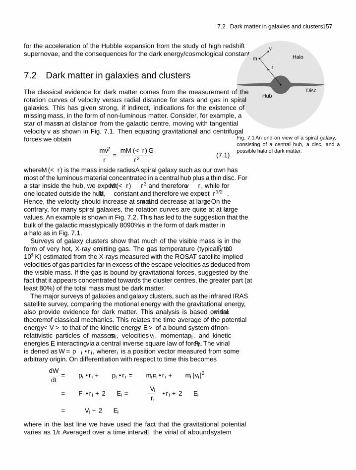
7.2 Dark matter in galaxies and clusters 157
for the acceleration of the Hubble expansion from the study of high redshiftsupernovae, and the consequences for the dark energy/cosmological constant.
7.2 Dark matter in galaxies and clusters
m
r
v
HubDisc
Halo
Fig. 7.1 An end-on view of a spiral galaxy,consisting of a central hub, a disc, and apossible halo of dark matter.
The classical evidence for dark matter comes from the measurement of therotation curves of velocity versus radial distance for stars and gas in spiralgalaxies. This has given strong, if indirect, indications for the existence of‘missing’ mass, in the form of non-luminous matter. Consider, for example, astar of mass m at distance r from the galactic centre, moving with tangentialvelocity v as shown in Fig. 7.1. Then equating gravitational and centrifugalforces we obtain
mv2
r= mM (< r) G
r2(7.1)
where M (< r) is the mass inside radius r. A spiral galaxy such as our own hasmost of the luminous material concentrated in a central hub plus a thin disc. Fora star inside the hub, we expect M (< r) ∝ r3 and therefore v ∝ r, while forone located outside the hub, M ∼ constant and therefore we expect v ∝ r−1/2.Hence, the velocity should increase at small r and decrease at large r. On thecontrary, for many spiral galaxies, the rotation curves are quite flat at large rvalues. An example is shown in Fig. 7.2. This has led to the suggestion that thebulk of the galactic mass—typically 80–90%—is in the form of dark matter ina halo as in Fig. 7.1.
Surveys of galaxy clusters show that much of the ‘visible’ mass is in theform of very hot, X-ray emitting gas. The gas temperature (typically 107 to108 K) estimated from the X-rays measured with the ROSAT satellite impliedvelocities of gas particles far in excess of the escape velocities as deduced fromthe visible mass. If the gas is bound by gravitational forces, suggested by thefact that it appears concentrated towards the cluster centres, the greater part (atleast 80%) of the total mass must be dark matter.
The major surveys of galaxies and galaxy clusters, such as the infrared IRASsatellite survey, comparing the motional energy with the gravitational energy,also provide evidence for dark matter. This analysis is based on the virialtheorem of classical mechanics. This relates the time average of the potentialenergy < V > to that of the kinetic energy < E > of a bound system of i non-relativistic particles of masses mi, velocities vi, momenta pi, and kineticenergies Ei, interacting via a central inverse square law of force, Fi. The virialis defined as W = �pi · ri, where ri is a position vector measured from somearbitrary origin. On differentiation with respect to time this becomes
dW
dt=∑
pi · ri +∑
pi · ri =∑
mi ri · ri +∑
mi |vi|2
=∑
Fi · ri + 2∑
Ei =∑(
∂Vi
∂ri
)· ri + 2
∑Ei
= −∑
Vi + 2∑
Ei
where in the last line we have used the fact that the gravitational potentialvaries as 1/r. Averaged over a time interval T , the virial of a bound system
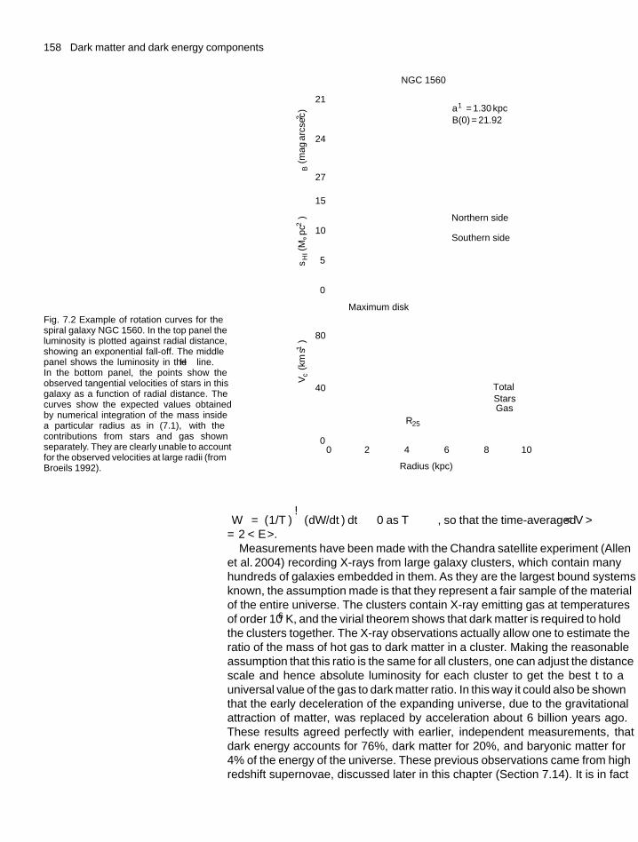
158 Dark matter and dark energy components
Fig. 7.2 Example of rotation curves for thespiral galaxy NGC 1560. In the top panel theluminosity is plotted against radial distance,showing an exponential fall-off. The middlepanel shows the luminosity in the Hα line.In the bottom panel, the points show theobserved tangential velocities of stars in thisgalaxy as a function of radial distance. Thecurves show the expected values obtainedby numerical integration of the mass insidea particular radius as in (7.1), with thecontributions from stars and gas shownseparately. They are clearly unable to accountfor the observed velocities at large radii (fromBroeils 1992).
NGC 1560
a–1 = 1.30 kpcB(0) = 21.92
Northern side
Southern side
Maximum disk
TotalStarsGas
00
40
80
2 4 6 8 10
R25
Vc (
kms–1
)0
5
10
15
27
24
21
sH
I(M
pc–2
)� B
(m
agar
csec
–2)
Radius (kpc)
〈W 〉 = (1/T )∫
(dW/dt) dt → 0 as T → ∞, so that the time-averaged <V >
= 2 <E >.Measurements have been made with the Chandra satellite experiment (Allen
et al. 2004) recording X-rays from large galaxy clusters, which contain manyhundreds of galaxies embedded in them. As they are the largest bound systemsknown, the assumption made is that they represent a fair sample of the materialof the entire universe. The clusters contain X-ray emitting gas at temperaturesof order 106 K, and the virial theorem shows that dark matter is required to holdthe clusters together. The X-ray observations actually allow one to estimate theratio of the mass of hot gas to dark matter in a cluster. Making the reasonableassumption that this ratio is the same for all clusters, one can adjust the distancescale and hence absolute luminosity for each cluster to get the best fit to auniversal value of the gas to dark matter ratio. In this way it could also be shownthat the early deceleration of the expanding universe, due to the gravitationalattraction of matter, was replaced by acceleration about 6 billion years ago.These results agreed perfectly with earlier, independent measurements, thatdark energy accounts for 76%, dark matter for 20%, and baryonic matter for4% of the energy of the universe. These previous observations came from highredshift supernovae, discussed later in this chapter (Section 7.14). It is in fact
7.3 Gravitational lensing 159
remarkable and heartening that quite different techniques for estimating thebasic parameters of the universe are in such good agreement.
Some of the most remarkable evidence for dark matter comes from theobservation of emission lines from very distant clouds of hydrogen, indicatingredshifts of z = 5 or 6, located in vast galaxies of what appears to be darkmatter, accounting for at least 99% of the total mass. Dark matter seems also tobe required from quite independent considerations of the level of fluctuationsin the cosmic microwave background and the growth of structure in the earlyuniverse, as discussed in Chapter 8. These density fluctuations are observedto be of order �ρ/ρ ∼ 10−5, and fluctuations 2–3 orders of magnitude largerwould have been necessary if formation of galaxy and galaxy clusters wasto be achieved by gravitational collapse of baryonic matter alone, once ithad decoupled from radiation at z ∼ 1000. On the other hand, as discussedin Section 5.13, the existence of (cold) dark matter with �cdm ∼ 0.20 wouldhave led to dominance of matter over radiation at a higher redshift (z ∼ 3000)and more effective gravitational collapse of matter (with the gravitational fieldof the dark matter dragging baryonic matter along with it) from a much earlierepoch.
Finally, the masses of galaxy clusters and the contribution of dark matter canbe estimated directly by their effects on the images of more distant quasars,due to the process of gravitational lensing, which is discussed in the followingsections. It has the advantage that it avoids some of the assumptions necessaryfor other methods.
7.3 Gravitational lensing
Very important information regarding the amount and location of dark matterhas come from gravitational lensing, which we therefore discuss at some length.The gravitational deflection of photons passing by a point mass M at a distanceof closest approach b was given in Section 2.6 by the formula (2.28):
α = 4GM
c2b(7.2)
This is the deflection predicted by Einstein’s general theory of relativity, beingexactly a factor 2 larger than the deflection one obtains according to Newtonianmechanics (see Problem 7.1). The correctness of the Einstein prediction wasfirst demonstrated by the 1919 solar eclipse expedition by Eddington to theisland of Principe, which measured the deflection of light from stars close tothe Sun’s limb.
The gravitational deflection of light implies that massive objects may act asgravitational lenses, as foreseen by Einstein even before the relation (7.2) hadbeen tested experimentally. Suppose in Fig. 7.3 that S is a source of light (star)and that the rays to the observer O pass close to a massive point lensing objectL of mass M . The diagram represents the situation in the plane defined by O,S, and L, and is the gravitational analogue of a thin lens system in optics. Inthe general case, the source and lens will not be collinear with the observerand there will then be two images of the source, S1 and S2. Then if α denotes
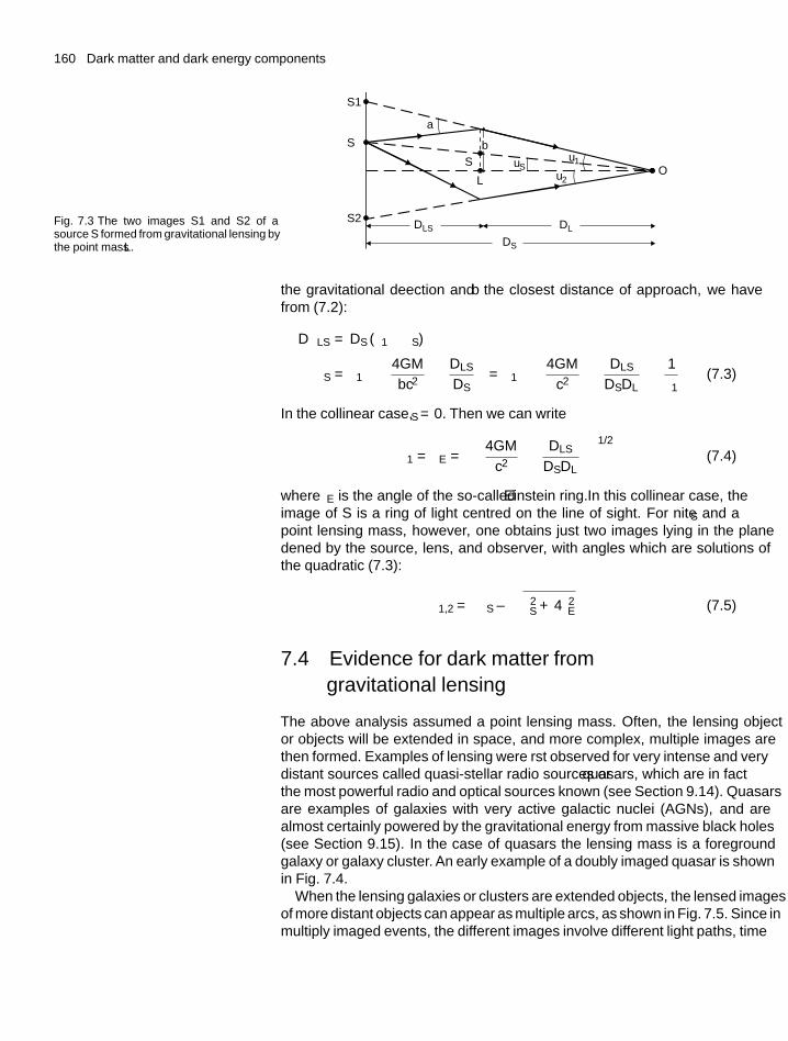
160 Dark matter and dark energy components
Fig. 7.3 The two images S1 and S2 of asource S formed from gravitational lensing bythe point mass L.
S1
S
S2 DLS
DS
DL
S�
L
b
O
a
uSu2
u1
the gravitational deflection and b the closest distance of approach, we havefrom (7.2):
αDLS = DS (θ1 − θS)
θS = θ1 −(
4GM
bc2
)(DLS
DS
)= θ1 −
(4GM
c2
)(DLS
DSDL
)(1
θ1
)(7.3)
In the collinear case, θS = 0. Then we can write
θ1 = θE =[(
4GM
c2
)(DLS
DSDL
)]1/2
(7.4)
where θE is the angle of the so-called Einstein ring. In this collinear case, theimage of S is a ring of light centred on the line of sight. For finite θS and apoint lensing mass, however, one obtains just two images lying in the planedefined by the source, lens, and observer, with angles which are solutions ofthe quadratic (7.3):
θ1,2 =[θS ±
√θ2
S + 4θ2E
](7.5)
7.4 Evidence for dark matter fromgravitational lensing
The above analysis assumed a point lensing mass. Often, the lensing objector objects will be extended in space, and more complex, multiple images arethen formed. Examples of lensing were first observed for very intense and verydistant sources called quasi-stellar radio sources or quasars, which are in factthe most powerful radio and optical sources known (see Section 9.14). Quasarsare examples of galaxies with very active galactic nuclei (AGNs), and arealmost certainly powered by the gravitational energy from massive black holes(see Section 9.15). In the case of quasars the lensing mass is a ‘foreground’galaxy or galaxy cluster. An early example of a doubly imaged quasar is shownin Fig. 7.4.
When the lensing galaxies or clusters are extended objects, the lensed imagesof more distant objects can appear as multiple arcs, as shown in Fig. 7.5. Since inmultiply imaged events, the different images involve different light paths, time
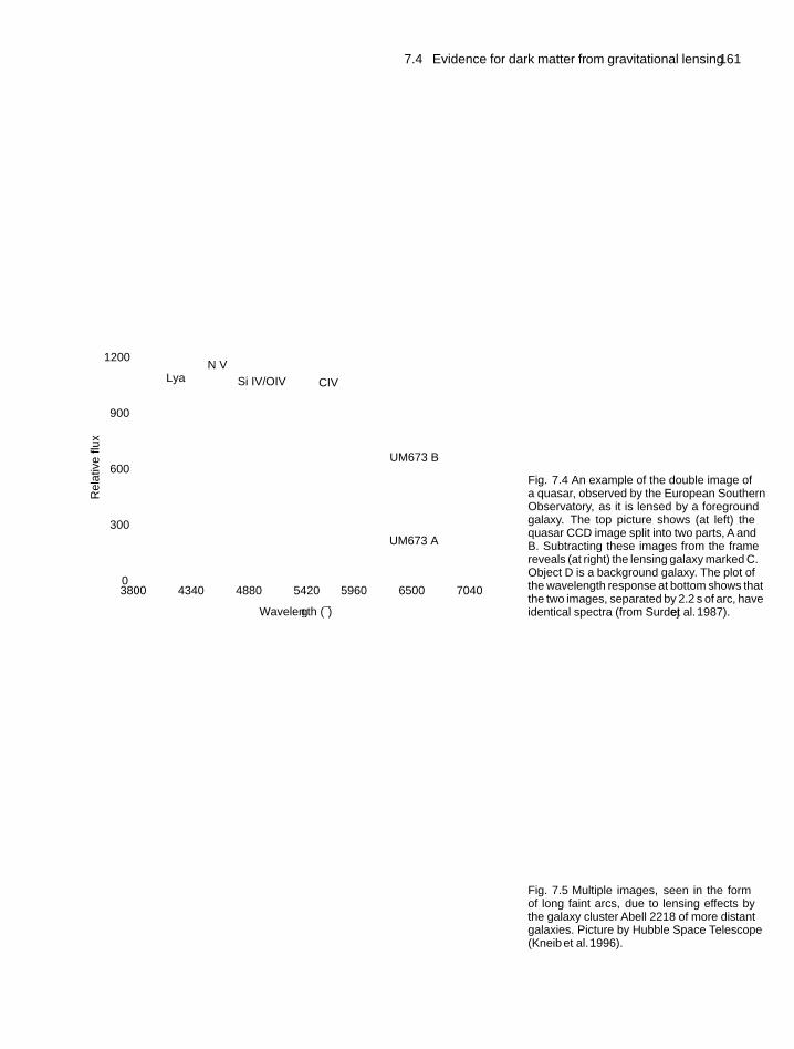
7.4 Evidence for dark matter from gravitational lensing 161
1200
900
600
300
3800 4340 4880 5420
Wavelength (Å)
5960 6500 70400
Rel
ativ
e fl
ux
UM673 A
UM673 B
CIVSi IV/OIV
N VLya
a b
AB
D
D
C
5"
Fig. 7.4 An example of the double image ofa quasar, observed by the European SouthernObservatory, as it is lensed by a foregroundgalaxy. The top picture shows (at left) thequasar CCD image split into two parts, A andB. Subtracting these images from the framereveals (at right) the lensing galaxy marked C.Object D is a background galaxy. The plot ofthe wavelength response at bottom shows thatthe two images, separated by 2.2 s of arc, haveidentical spectra (from Surdej et al. 1987).
Fig. 7.5 Multiple images, seen in the formof long faint arcs, due to lensing effects bythe galaxy cluster Abell 2218 of more distantgalaxies. Picture by Hubble Space Telescope(Kneib et al. 1996).
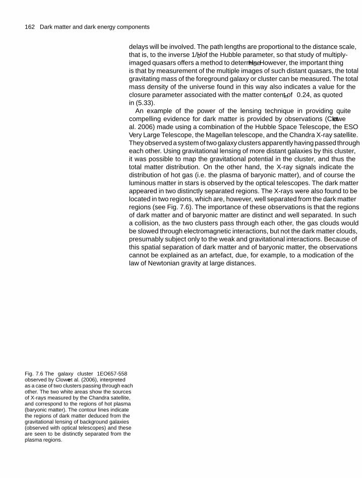
162 Dark matter and dark energy components
delays will be involved. The path lengths are proportional to the distance scale,that is, to the inverse 1/H0 of the Hubble parameter, so that study of multiply-imaged quasars offers a method to determine H0. However, the important thingis that by measurement of the multiple images of such distant quasars, the totalgravitating mass of the foreground galaxy or cluster can be measured. The totalmass density of the universe found in this way also indicates a value for theclosure parameter associated with the matter content of �m ≈ 0.24, as quotedin (5.33).
An example of the power of the lensing technique in providing quitecompelling evidence for dark matter is provided by observations (Clowe etal. 2006) made using a combination of the Hubble Space Telescope, the ESOVery Large Telescope, the Magellan telescope, and the Chandra X-ray satellite.They observed a system of two galaxy clusters apparently having passed througheach other. Using gravitational lensing of more distant galaxies by this cluster,it was possible to map the gravitational potential in the cluster, and thus thetotal matter distribution. On the other hand, the X-ray signals indicate thedistribution of hot gas (i.e. the plasma of baryonic matter), and of course theluminous matter in stars is observed by the optical telescopes. The dark matterappeared in two distinctly separated regions. The X-rays were also found to belocated in two regions, which are, however, well separated from the dark matterregions (see Fig. 7.6). The importance of these observations is that the regionsof dark matter and of baryonic matter are distinct and well separated. In sucha collision, as the two clusters pass through each other, the gas clouds wouldbe slowed through electromagnetic interactions, but not the dark matter clouds,presumably subject only to the weak and gravitational interactions. Because ofthis spatial separation of dark matter and of baryonic matter, the observationscannot be explained as an artefact, due, for example, to a modification of thelaw of Newtonian gravity at large distances.
Fig. 7.6 The galaxy cluster 1EO657-558observed by Clowe et al. (2006), interpretedas a case of two clusters passing through eachother. The two white areas show the sourcesof X-rays measured by the Chandra satellite,and correspond to the regions of hot plasma(baryonic matter). The contour lines indicatethe regions of dark matter deduced from thegravitational lensing of background galaxies(observed with optical telescopes) and theseare seen to be distinctly separated from theplasma regions.
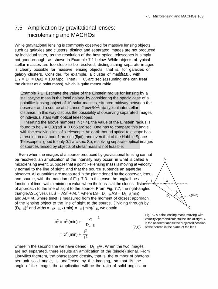
7.5 Microlensing and MACHOs 163
7.5 Amplification by gravitational lenses:microlensing and MACHOs
While gravitational lensing is commonly observed for massive lensing objectssuch as galaxies and clusters, distinct and separated images are not producedby individual stars, as the resolution of the best optical telescopes is simplynot good enough, as shown in Example 7.1 below. While objects of typicalstellar masses are too close to be resolved, distinguishing separate imagesis clearly possible for massive lensing objects, that is, for galaxies orgalaxy clusters. Consider, for example, a cluster of mass 1014Msun, withDLS = DL = DS/2 = 100 Mpc. Then θE ∼ 65 arc sec (assuming one can treatthe cluster as a point mass), which is quite measurable.
Example 7.1 Estimate the value of the Einstein radius for lensing by astellar-type mass in the local galaxy, by considering the specific case of apointlike lensing object of 10 solar masses, situated midway between theobserver and a source at distance 2 pc (6 × 10¹⁶m)—a typical interstellardistance. In this way discuss the possibility of observing separated imagesof individual stars with optical telescopes.
Inserting the above numbers in (7.4), the value of the Einstein radius isfound to be θE = 0.32μrad = 0.065 arc sec. One has to compare this anglewith the resolving limit of a telescope. An earth-bound optical telescope hasa resolution of about 1 arc sec (5μ rad), and even that of the Hubble SpaceTelescope is good to only 0.1 arc sec. So, resolving separate optical imagesof sources lensed by objects of stellar mass is not feasible.
Even when the images of a source produced by gravitational lensing cannotbe resolved, an amplification of the intensity may occur, in what is called amicrolensing event. Suppose that a pointlike lensing mass is moving at velocityv normal to the line of sight, and that the source subtends an angle θS at theobserver. All quantities are measured in the plane defined by the observer, lens,and source, with the notation of Fig. 7.3. In this case the angle θS will be afunction of time, with a minimum value when the lens is at the closest distanceof approach to the line of sight to the source. From Fig. 7.7, the right-angledtriangleAS′L gives us LS′2 =AS′2+AL2, where LS′ = DLθs,AS′ = DLθs(min),and AL= vt, where time t is measured from the moment of closest approachof the lensing object to the line of sight to the source. Dividing through by(DLθE)2 and with x = θS/θE, x (min) = θS (min)/θE, we obtain 0
DL
A
S�
v L
�S
�S (min)
Fig. 7.7 A point lensing mass L moving withvelocity v perpendicular to the line of sight. Ois the observer and S′ is the projected positionof the source in the plane of the lens.
x2 = x2 (min) +(
vt
DLθE
)2
= x2 (min) + t2
T 2
(7.6)
where in the second line we have defined T = DLθE/v. When the two imagesare not separated, there results an amplification of the (single) signal. FromLiouville’s theorem, the phase–space density, that is, the number of photonsper unit solid angle, is unaffected by the imaging, so that if θ is theangle of the image, the amplification will be the ratio of solid angles, or
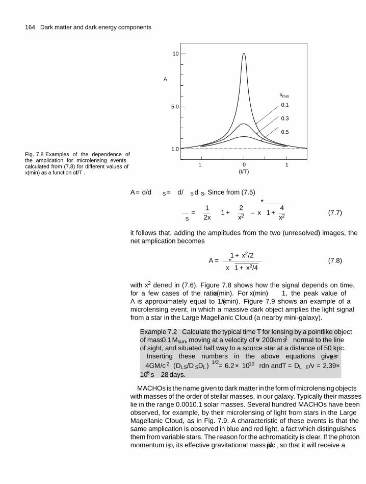
164 Dark matter and dark energy components
Fig. 7.8 Examples of the dependence ofthe amplification for microlensing eventscalculated from (7.8) for different values ofx(min) as a function of t/T .
–1 0 1(t/T )
A
0.1
0.3
0.5
xmin
10
5.0
1.0
A = d�/d�S = θ dθ/θS dθS. Since from (7.5)
θ
θS=(
1
2x
)[1 +(
2
x2
)± x
√1 + 4
x2
](7.7)
it follows that, adding the amplitudes from the two (unresolved) images, thenet amplification becomes
A =(1 + x2/2
)[x√
1 + x2/4] (7.8)
with x2 defined in (7.6). Figure 7.8 shows how the signal depends on time,for a few cases of the ratio x(min). For x(min) 1, the peak value ofA is approximately equal to 1/x (min). Figure 7.9 shows an example of amicrolensing event, in which a massive dark object amplifies the light signalfrom a star in the Large Magellanic Cloud (a nearby mini-galaxy).
Example 7.2 Calculate the typical time T for lensing by a pointlike objectof mass 0.1 Msun, moving at a velocity of v = 200 km s−1 normal to the lineof sight, and situated half way to a source star at a distance of 50 kpc.
Inserting these numbers in the above equations gives θE =[(4GM /c2
)(DLS/DSDL)
]1/2= 6.2 × 10⁻¹⁰ rdn and T = DLθE/v = 2.39 ×10⁶ s ∼ 28 days.
MACHOs is the name given to dark matter in the form of microlensing objectswith masses of the order of stellar masses, in our galaxy. Typically their masseslie in the range 0.001–0.1 solar masses. Several hundred MACHOs have beenobserved, for example, by their microlensing of light from stars in the LargeMagellanic Cloud, as in Fig. 7.9. A characteristic of these events is that thesame amplification is observed in blue and red light, a fact which distinguishesthem from variable stars. The reason for the achromaticity is clear. If the photonmomentum is p, its effective gravitational mass is p/c, so that it will receive a
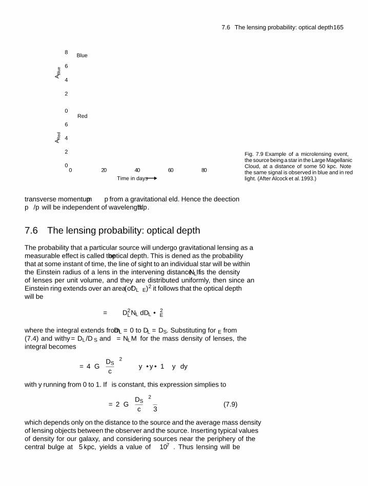
7.6 The lensing probability: optical depth 165
Blue
Red
AB
lue
AR
ed
8
6
4
2
0
6
4
2
00 20 40 60 80
Time in days
Fig. 7.9 Example of a microlensing event,the source being a star in the Large MagellanicCloud, at a distance of some 50 kpc. Notethe same signal is observed in blue and in redlight. (After Alcock et al. 1993.)
transverse momentum �p ∝ p from a gravitational field. Hence the deflection�p/p will be independent of wavelength h/p.
7.6 The lensing probability: optical depth
The probability that a particular source will undergo gravitational lensing as ameasurable effect is called the optical depth. This is defined as the probabilitythat at some instant of time, the line of sight to an individual star will be withinthe Einstein radius of a lens in the intervening distance. If NL is the densityof lenses per unit volume, and they are distributed uniformly, then since anEinstein ring extends over an area of π(DLθE)2 it follows that the optical depthwill be
τ =∫
πD2LNL dDL · θ2
E
where the integral extends from DL = 0 to DL = DS. Substituting for θE from(7.4) and with y = DL/DS and ρ = NLM for the mass density of lenses, theintegral becomes
τ = 4πG
(DS
c
)2 ∫ρ(y) · y · (1 − y
)dy
with y running from 0 to 1. If ρ is constant, this expression simplifies to
τ = 2πG
(DS
c
)2ρ
3(7.9)
which depends only on the distance to the source and the average mass densityof lensing objects between the observer and the source. Inserting typical valuesof density for our galaxy, and considering sources near the periphery of thecentral bulge at ∼ 5 kpc, yields a value of τ ∼ 10−7. Thus lensing will be
166 Dark matter and dark energy components
a comparatively rare occurrence, and to detect dark matter in the form of‘dark stars’—that is, MACHOs as described above—one needs to examinethe light curves of many millions of stars over months and years. This hasrequired computerized search techniques, of the type first used in the oldautomated analysis systems in scanning bubble chamber film in particle physicsexperiments.
The magnitude of the magnification involved in microlensing varies inverselyas the impact parameter between the lensed star and the MACHO, and sodetection of microlensing typically involves examination of millions of stars,as discussed above. On the other hand, the Shapiro time delay falls off onlylogarithmically with impact parameter, so even with only a few thousandknown pulsars, an effect may be detectable, although so far none has beenclaimed.
The present evidence is that MACHOs appear to account for only a smallfraction of all the baryonic matter. The majority is in the form of stars, gas,and dust, of which by far the greatest contribution is from gas—commonly thevery hot, X-ray emitting gas inhabiting galactic clusters, as discussed below.Certainly, MACHOs make only a trivial contribution to the energy densityof dark matter. We now discuss some of the various candidates which havebeen proposed to constitute dark matter, as well as the experimental methodsemployed to search for them.
7.7 Baryonic dark matter
What is the nature of the dark matter which has been postulated to account forthe phenomena described above? Some of the dark matter must be baryonic,since the value �baryon ≈ 0.04 deduced from nucleosynthesis in the Big Bangis almost an order of magnitude larger than the closure parameter associatedwith visible stars, gas, and dust, of �lum ∼ 0.01—see (5.31). In our own galaxy,some at least of this non-luminous baryonic dark matter has been accounted forin the form of compact halo objects (MACHOs) described above. However,X-ray studies of galaxy clusters reveal vast amounts of gas present between thegalaxies in such clusters, and it seems possible that this accounts for almost halfof the baryonic matter in the universe. Recent observations with the ChandraX-ray satellite, of absorption lines of oxygen and nitrogen, suggest that theother sources of the missing baryons are long filaments of gas associated withblazars (see Sections 9.10 and 9.14), which are AGN sources of TeV γ-rays.
There are no indications at present that more exotic baryonic objects such asmini black holes contribute significantly to the baryonic energy density. On thecontrary, any primordial mini black holes of M <1011kg would have lifetimesless than the age of the universe, and in evaporating would emit Hawkingradiation (as γ-rays)—see Sections 10.11 and 10.12. From the observed flux ofγ-radiation from all sources one can set an upper limit on the energy density ofsuch black holes of �BH<10−7.
In summary, baryonic matter makes only a small contribution to the overalldensity of the universe, and certainly less than 15% of the total estimated densityof dark matter.
7.8 Neutrinos 167
7.8 Neutrinos
The presently favoured hypothesis is that non-baryonic dark matter is composedof elementary particles, created at an early hot stage of the universe, and stableenough to have survived to the present day. The nature of such particles ispresently a total mystery, although suggestions abound. To begin with, wecan try to eliminate some known candidates. As indicated in Section 5.12,the neutrinos νe, νμ, and ντ and their antiparticles, together with electrons,positrons, and photons would have been produced prolifically in the earlyuniverse, and present in comparable numbers, according to the equilibriumreactions in (5.60):
γ ↔ e+ + e− ↔ vi + vi
where i = e, μ, τ. As explained in Chapter 5, neutrinos would have frozen-out from further (weak) interactions with electrons or other matter when kT hadfallen below about 3 MeV. Before better laboratory evidence on the smallness ofneutrino masses became available, in the middle of the 1990s, the question aroseas to whether neutrinos could be substantial—or even dominant—contributorsto dark matter. In this respect they had the great advantage that they were at leastknown to exist. As discussed in Section 5.11, the relic microwave neutrino (plusantineutrino) number density would be comparable with the relic microwavephoton number density, with a value (see (5.67)):
Nv =(
3
11
)Nγ = 113 cm−3 (7.10)
per neutrino flavour, to be compared with a number density of 411 cm−3 forthe microwave photons. We note from this number density that the total energydensity of neutrinos would be equal to the critical density (5.26) if the sum ofthe masses of the three flavours had the value∑
e,μ,τ
mvc2 = 47 eV (7.11)
So neutrinos with masses in the few eV mass range could make significantcontributions to dark matter. However, evidence from neutrino oscillations(Section 4.2) indicates very much smaller masses than in (7.11), below 0.1 eV/c2
as judged from the mass differences. Another problem with neutrinos as darkmatter candidates is that they would constitute ‘hot’dark matter. With the criticaltemperature of kT ∼ 3 MeV, neutrinos were relativistic when they decoupledfrom other matter and also when the structures in the universe were forming.Consequently, they would stream away rapidly and, just like the photons, tendto iron out any primordial density fluctuations. So if large-scale structures areto form, early computer simulations indicated that the fraction of dark matterwhich is ‘hot’ could only be of order 30% or less. All this will be discussed indetail in Sections 8.9–8.11.
Aside from the question of relic neutrinos forming dark matter, the existenceinferred above of some 340 neutrinos in each cubic centimetre throughoutspace, with energies in the milli-electron volt range, poses a truly formidable
168 Dark matter and dark energy components
challenge to the experimentalist to detect them. After microwave photons, therelic neutrinos are, as far as we know, by far the most prolific particles inthe universe, but there seems to be no obvious way to show their existence.Since the value Tν = 1.9 K given in Section 5.11 implies, together with the dataon mass differences in Section 4.2, that the relic neutrinos (or at least two ofthe three flavours) are non-relativistic, their de Broglie wavelengths will be oforder 0.5 mm, so they could be coherently scattered by sizeable lumps of matter.However, so far no really plausible method of detecting them has been found,although several ideas have been put forward. For example, the Pauli principlecould cause suppression of weak decays resulting in emitted neutrinos trying tooccupy the same cells of phase space as the relic neutrinos. It is also remotelypossible that, if ultra-high energy (1023 eV!) neutrino sources actually exist,their spectrum might show a detectable dip where such neutrinos interact withthe relic (anti)neutrinos to form the resonance v + v → Z0. But all such ideasseem to be for the far future.
The foregoing discussion of course applies to the ‘light’neutrinos νe, νμ, andντ we are familiar with in the laboratory. There is the additional possibilityof extremely massive (GUT scale) Majorana neutrinos being created at a veryearly stage of the universe, as discussed in Section 4.4. These could have playeda vital role in the development of the universal matter–antimatter asymmetry.However, such massive neutrinos would be unstable and have disappeared bydecay, and could not have contributed to dark matter today.
7.9 Axions
The axion is a very light pseudoscalar particle (spin-parity 0−) originallypostulated in connection with the absence of CP violation in strong interactions(quantum chromodynamics,QCD). In principle, complex phases can occurin the quark wavefunctions in QCD, and these would be T violating or CPviolating (as indeed they are in the weak interaction sector). However, theupper limit to the electric dipole moment of the neutron is nine orders ofmagnitude less than strong CP violation predicts. To cancel this undesirablefeature and to account for the smallness of any possible violation, Peccei andQuinn (1977) proposed a new global U(1) symmetry, spontaneously brokenat some very-high-energy scale, and giving rise to an associated boson (aso-called Goldstone boson) called the axion, which receives a small massvia non-perturbative (instanton) effects at phase transitions on the QCD scale(200 GeV). The axion, just like the pseudoscalar neutral pion, can decay intotwo photons, at a rate determined by the extremely weak coupling 1/fa toother particles, where fa is the Peccei-Quinn energy scale (all quantities hereare expressed in ‘natural units’ h = c = 1). The axion mass is given by theformula
ma ≈ 0.5mπfπ
fa≈ 6 eV[
fa/(106 GeV
)] (7.12)
where fπ = 93 MeV is the pion decay constant. Thus a value of ma = 1 (0.01)eV/c2 would correspond to fa = 6 × 10⁶ (6 × 10⁸) GeV. The actual lifetime foraxion decay to two photons is proportional to 1/m5
a and exceeds the age of the
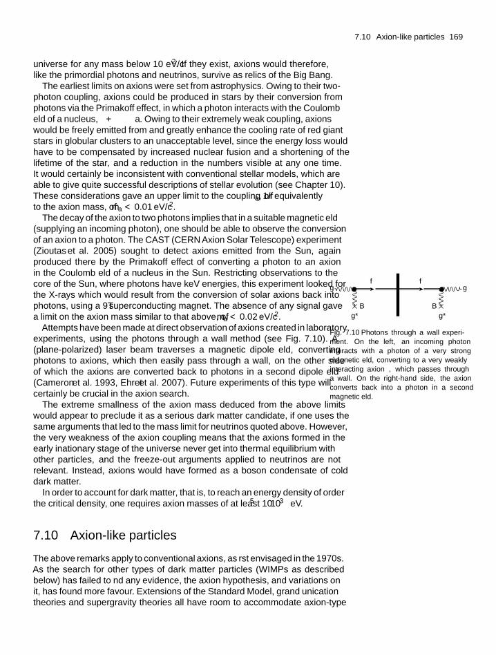
7.10 Axion-like particles 169
universe for any mass below 10 eV/c2. If they exist, axions would therefore,like the primordial photons and neutrinos, survive as relics of the Big Bang.
The earliest limits on axions were set from astrophysics. Owing to their two-photon coupling, axions could be produced in stars by their conversion fromphotons via the Primakoff effect, in which a photon interacts with the Coulombfield of a nucleus, γ +γ → a. Owing to their extremely weak coupling, axionswould be freely emitted from and greatly enhance the cooling rate of red giantstars in globular clusters to an unacceptable level, since the energy loss wouldhave to be compensated by increased nuclear fusion and a shortening of thelifetime of the star, and a reduction in the numbers visible at any one time.It would certainly be inconsistent with conventional stellar models, which areable to give quite successful descriptions of stellar evolution (see Chapter 10).These considerations gave an upper limit to the coupling 1/fa, or equivalentlyto the axion mass, of ma < 0.01 eV/c2.
The decay of the axion to two photons implies that in a suitable magnetic field(supplying an incoming photon), one should be able to observe the conversionof an axion to a photon. The CAST (CERN Axion Solar Telescope) experiment(Zioutas et al. 2005) sought to detect axions emitted from the Sun, againproduced there by the Primakoff effect of converting a photon to an axionin the Coulomb field of a nucleus in the Sun. Restricting observations to thecore of the Sun, where photons have keV energies, this experiment looked forthe X-rays which would result from the conversion of solar axions back intophotons, using a 9T superconducting magnet. The absence of any signal gavea limit on the axion mass similar to that above, of ma < 0.02 eV/c2.
f
g*
g g
g*
f
B B
Fig. 7.10 ‘Photons through a wall’ experi-ment. On the left, an incoming photoninteracts with a photon of a very strongmagnetic field, converting to a very weaklyinteracting axion φ, which passes througha wall. On the right-hand side, the axionconverts back into a photon in a secondmagnetic field.
Attempts have been made at direct observation of axions created in laboratoryexperiments, using the ‘photons through a wall’ method (see Fig. 7.10). A(plane-polarized) laser beam traverses a magnetic dipole field, convertingphotons to axions, which then easily pass through a wall, on the other sideof which the axions are converted back to photons in a second dipole field(Cameron et al. 1993, Ehret et al. 2007). Future experiments of this type willcertainly be crucial in the axion search.
The extreme smallness of the axion mass deduced from the above limitswould appear to preclude it as a serious dark matter candidate, if one uses thesame arguments that led to the mass limit for neutrinos quoted above. However,the very weakness of the axion coupling means that the axions formed in theearly inflationary stage of the universe never get into thermal equilibrium withother particles, and the ‘freeze-out’ arguments applied to neutrinos are notrelevant. Instead, axions would have formed as a boson condensate of colddark matter.
In order to account for dark matter, that is, to reach an energy density of orderthe critical density, one requires axion masses of at least 10−5 − 10−3 eV.
7.10 Axion-like particles
The above remarks apply to conventional axions, as first envisaged in the 1970s.As the search for other types of dark matter particles (WIMPs as describedbelow) has failed to find any evidence, the axion hypothesis, and variations onit, has found more favour. Extensions of the Standard Model, grand unificationtheories and supergravity theories all have room to accommodate axion-type
170 Dark matter and dark energy components
particles. Indeed, the definition of axion can encompass particles with somewhatdifferent properties, for example, scalar rather than pseudoscalar particles,and particles which do not couple directly to quarks or leptons. Furthermore,depending on the properties assumed, such particles can form either cold orhot dark matter. They are referred to as axion-like particles (ALPs) and thecouplings are no longer related to the axion masses as in (7.12).
In the so-called hadronic axion models, axions have no first order couplingto leptons or quarks, in which case the foregoing mass limits do not apply. Theaxion is coupled to hadrons, for example, to pions in the process a + π → π + π.In this case, thermalization of the axions after the temperature falls below theQCD scale of ∼ 100 GeV can take place, and similar arguments to those forneutrinos on freeze-out rates will then apply. The present axion intensity wouldbe of the same order as for relic neutrinos, and if the axion mass is in theeV mass range, the axion could again make an important contribution to darkmatter. However, the crucial experiments definitely demonstrating the existenceof axions, hot or cold, still remain to be done.
7.11 Weakly interacting massive particles
The other favoured hypothesis for dark matter particles is that they are weaklyinteracting massive particles (WIMPs), moving with non-relativistic velocitiesat the time of freeze-out and thus constituting cold dark matter.
First, however, we should ask if these particles could be massive neutrinos. Ifthey were, and had masses such that they were still relativistic at freeze-out, theclosure parameter would increase with neutrino mass mν as in (7.11), and formν ∼ 1 MeV, would reach the unphysical value of � ∼ 104. For higher masses,the heavy neutrinos would become non-relativistic at decoupling, and as shownbelow, this then results in � ∝ 1/m2
v instead of � ∝ mν. The closure parameterfalls back below � = 1 for a mass above 3 GeV. So the fact that the measuredvalue of � is not large compared with unity, excludes the mass range 50 eV–3GeV, while experiments at the LEP electron–positron collider at CERN proveconclusively that there are no ‘extra’ conventional neutrinos of mass below(1/2)MZ = 45 GeV. Conventional neutrinos of mν > 45 GeV, if they existed,would, however, make no significant contribution to � (< 0.01, from the 1/m2
vdependence). The dependence of the closure parameter on mass is illustratedin Fig. 7.11, drawn for WIMPs generally, that is, for massive non-relativisticparticles with conventional weak couplings.
For several reasons, it is considered that supersymmetric (SUSY) particlescould be the most likely WIMP candidates. As described in Section 4.5, suchSUSY particles are expected to be created in pairs, with opposite values R = ±1of a conserved quantum number called R-parity. Heavier SUSY particles woulddecay to lighter ones in R-conserving processes, ultimately ending up with thelightest supersymmetric particle (LSP), which we denote by the symbol χ.This particle is assumed to be stable and therefore to have survived from theprimordial era of the universe. The LSP is usually identified with the neutralino,a neutral fermion which is the lightest of the states arising from a linearcombination of the photino, zino, and two higgsinos (see Table 4.1). Since suchanomalously heavy particles are not constituents of atoms or nuclei, they cannothave either electromagnetic or strong coupling and are assumed to interactonly weakly. Although neutralinos are stable, they can of course disappear
7.11 Weakly interacting massive particles 171
by annihilation with their antiparticles, which will have been generated withthe same abundance as the particles. There are many free parameters in SUSYmodels, which means that the LSP mass as well as the annihilation cross-sectionand cosmological abundance can vary over quite wide ranges, and it is probablythis flexibility which is part of the attraction of such models.
Let us now look more closely at the constraints which WIMP models haveto fulfil. First, we are searching for cold dark matter, since this must form thebulk of all dark matter if one is to successfully account for the development ofstructures in the universe, as explained in Chapter 8. So the WIMPs must benon-relativistic when they ‘freeze-out’. This freeze-out occurs when the rate ofχχ annihilation falls below the expansion rate, that is, when
N 〈σv〉 ≤ H (7.13)
where N is the WIMP number density, v is the relative velocity of particle andantiparticle, σ is the WIMP–antiWIMP annihilation cross-section, and H isthe Hubble parameter at the time of freeze-out. It will be seen that the WIMPabundance varies inversely as the annihilation cross-section, so that weakerinteractions lead to earlier freeze-out and consequently higher densities andlarger contributions to the closure parameter. Since the WIMPs are massive andnon-relativistic, M � T where M is the WIMP mass and T is the temperatureat freeze-out in energy units. Then the density will be given by the Boltzmannrelation (see Problem 5.3):
N (T ) =(
MT
2π
)3/2
exp
(−M
T
)(7.14)
The exact value of the χχ annihilation cross-section is of course unknown,but if it is of the same order as the weak cross-section then on dimensionalgrounds we could set < σv > ∼ G2
F M 2—see (1.27). Inserting (7.14) in (7.13)and with H = 1.66g ∗1/2 T 2/MPL as given by (5.59) in the radiation-dominateduniverse, the freeze-out condition becomes
(MT )3/2 exp
(−M
T
)G2
FM 2 ≤ fT 2
MPL(7.15)
where f includes the numerical constants involved and is of order 100. TheFermi constant squared is G2
F ≈ 10−10 GeV−4 while the Planck mass MPL ≈1019GeV. Inserting these numbers, one can easily solve numerically for thevalue of P = M /T at freeze-out. It varies slowly and logarithmically, fromaround P = 20 for M = 1 GeV to around P = 30 for M = 100 GeV. In thefollowing we take this ratio as a constant, P = 25. Now going back to (7.13),and recalling that the expansion parameter R ∝ 1/T , the WIMP density N (0)today, when the CMB temperature is T0 = 2.73 K, will be
N (0) ∼ (T0/T )3 × (T 2/MPL)
〈σv〉 (7.16)
The corresponding WIMP energy density will be
ρWIMP = MN (0) ∼ PT 30
(MPL 〈σv〉) ∼ 6 × 10⁻³¹
〈σv〉 GeV s−1
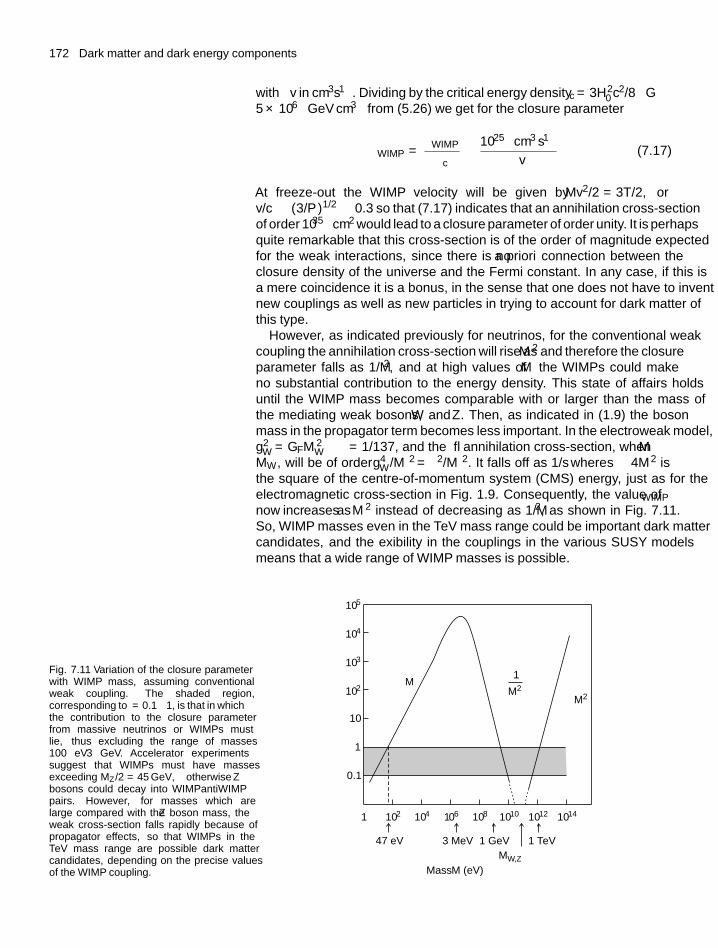
172 Dark matter and dark energy components
with σv in cm3s−1. Dividing by the critical energy density ρc = 3H 20 c2/8πG ≈
5 × 10⁻⁶ GeV cm−3 from (5.26) we get for the closure parameter
�WIMP = ρWIMP
ρc∼ 10−25 cm3 s−1
〈σv〉 (7.17)
At freeze-out the WIMP velocity will be given by Mv2/2 = 3T/2, orv/c ∼ (3/P)1/2 ∼ 0.3 so that (7.17) indicates that an annihilation cross-sectionof order 10−35 cm2 would lead to a closure parameter of order unity. It is perhapsquite remarkable that this cross-section is of the order of magnitude expectedfor the weak interactions, since there is no a priori connection between theclosure density of the universe and the Fermi constant. In any case, if this isa mere coincidence it is a bonus, in the sense that one does not have to inventnew couplings as well as new particles in trying to account for dark matter ofthis type.
However, as indicated previously for neutrinos, for the conventional weakcoupling the annihilation cross-section will rise as M 2 and therefore the closureparameter falls as 1/M 2, and at high values of M the WIMPs could makeno substantial contribution to the energy density. This state of affairs holdsuntil the WIMP mass becomes comparable with or larger than the mass ofthe mediating weak bosons, W and Z . Then, as indicated in (1.9) the bosonmass in the propagator term becomes less important. In the electroweak model,g2
W = GFM 2W ∼ α = 1/137, and the χχ annihilation cross-section, when M �
MW , will be of order g4W /M 2 = α2/M 2. It falls off as 1/s where s ∼ 4M 2 is
the square of the centre-of-momentum system (CMS) energy, just as for theelectromagnetic cross-section in Fig. 1.9. Consequently, the value of �WIMP
now increases as M 2 instead of decreasing as 1/M 2, as shown in Fig. 7.11.So, WIMP masses even in the TeV mass range could be important dark mattercandidates, and the flexibility in the couplings in the various SUSY modelsmeans that a wide range of WIMP masses is possible.
Fig. 7.11 Variation of the closure parameterwith WIMP mass, assuming conventionalweak coupling. The shaded region,corresponding to � = 0.1−1, is that in whichthe contribution to the closure parameterfrom massive neutrinos or WIMPs mustlie, thus excluding the range of masses100 eV–3 GeV. Accelerator experimentssuggest that WIMPs must have massesexceeding MZ/2 = 45 GeV, otherwise Zbosons could decay into WIMP–antiWIMPpairs. However, for masses which arelarge compared with the Z boson mass, theweak cross-section falls rapidly because ofpropagator effects, so that WIMPs in theTeV mass range are possible dark mattercandidates, depending on the precise valuesof the WIMP coupling.
104 108 1012 10141021 106 1010
47 eV 3 MeV
Mass M (eV)
1 GeV 1 TeVMW,Z
Ω � M
Ω � M2
Ω �M2
1
104
105
103
102
1
0.1
10Ω
7.12 Expected WIMP cross-sections and event rates 173
7.12 Expected WIMP cross-sectionsand event rates
There are two distinct possibilities for detection of WIMPs. Direct detectionof dark matter relies on observation of the scattering or other interaction of theWIMPs inside the detector, while indirect detection relies on the observation ofthe annihilation products of WIMPs in, for example, the halo of the galaxy, oras a result of their accumulation in the core of the Sun or the Earth. In the lattercases of course, the only secondary products which could be detected would beneutrinos. In fact, no evidence for an extra flux of high-energy neutrinos fromthe direction of the Sun or from the Earth’s core has ever been found.
In the case of direct detection, the WIMP rate may be expected to exhibitsome angular and time dependence. For example, if WIMPs predominantlypopulate the galactic halo, there might be a daily modulation because of theshadowing effects of the Earth when turned away from the galactic centre.An annual modulation in the event rate would also be expected as the Earth’sorbital velocity around the Sun adds to or subtracts from the velocity of the SolarSystem with respect to the galactic centre, so that both the velocity distributionof WIMPs and the cross-section for detection change with time.
We now discuss the expectations for elastic scattering of WIMPs by nuclei inthe detector, signalled by the nuclear recoil. The WIMP velocities are expectedto be of the order of galactic escape velocities, that is, v ∼ 10−3c, so that wecan use non-relativistic kinematics. Then if E = Mv2/2 is the kinetic energy ofa WIMP of mass M , colliding with a nucleus of mass MN = mA where A is themass number and m the nucleon mass, it is straightforward to show that the totalCMS energy is (if required, refer to Chapter 2 for relativistic transformations):
ε =[(M + MN)2 + 2MNE
]1/2
≈ [M + MN][
1 + MNE
(MN + M )2
] (7.18)
where in the second line we use the fact that E MN or M . If p* denotesthe (equal and opposite) momentum of each particle in the CMS, then in thenon-relativistic approximation
ε =(
MN + p∗2
2MN
)+(
M + p∗2
2M
)(7.19)
so these two equations give
p∗2 = 2μ2E
M= μ2v2 (7.20)
where μ = MNM /(MN + M ) is the reduced mass. The laboratory kineticenergy Er of the recoiling nucleus is maximum when its CMS vector momentumis reversed in the collision, so that it is scattered in the forward direction withlaboratory momentum 2p* and Er (max) = 2p∗2/MN = 2μ2v2/MN. This has avalue varying from v2MN/2 when MN = M to 2v2MN when M � MN. Sincethe CMS angular distribution at these low velocities will be isotropic, the recoilenergy distribution will vary uniformly between zero and Er(max). So with
174 Dark matter and dark energy components
v ∼ 10−3c and MN ∼ A GeV, we obtain recoil energies Er ∼ A keV or less.Hence, a sensitive detector is needed to observe such small recoil energies.
The scattering cross-section of the target nucleus depends on details of theSUSY model parameterization. For guidance we again assume a conventionalweak cross-section. From (1.18) with |Tif | = GF the cross-section per targetnucleus will be
σ ≈ G2Fp∗2K
πv2r
= G2Fμ2K
π(7.21)
where the relative velocity of incident particle and target nucleus in the CMS isvr = v = p∗/μ. The quantity K is a numerical model-dependent factor. For spin-independent coupling, the scattering amplitudes from the different nucleons inthe target nucleus should add coherently, so that K will contain a factor A2.However, the momentum transfer is of order p∗ = μv ∼ 10−3A GeV, while thenuclear radius R = 1.4A1/3 fm ∼ 7A1/3 GeV−1. The nucleus can only recoilcoherently if p*R 1, or A 50, otherwise K will contain a suppressionfactor (the square of the so-called form-factor).
The other possibility is spin-dependent (axial–vector) coupling, for whichthe amplitudes from different nucleons do not add since most of the nucleonspins cancel out, and the cross-section is smaller by a factor of order A2 thanthat for coherent scattering. As examples, for WIMPs identified with sneutrinos(see Table 4.1) the interaction is scalar and coherent, while if the WIMP is theLSP (neutralino) with spin 1/2, the interaction will be mostly incoherent.
The event rate to be expected depends on the WIMP number density andthe scattering cross-section. Because of their gravitational concentration in thegalaxy and particularly the disc and halo, the WIMP energy density in the solarsystem is estimated to be some 105 times that in the universe at large, atρWIMP ∼0.3 GeV cm−3, yielding a flux of ϕWIMP ∼ 0.3v/M cm−2 s−1, where the WIMPmass M is in GeV. The reaction rate per target nucleus will be W = σϕWIMP asin (1.14) and the event rate per unit target mass from (7.21) will be
R = W
MN∼ 10K
AMevents kg−1 day−1 (7.22)
Typical values of M = 100 GeV and A = 20 predict R ∼ 0.01 events per kgday for incoherent scattering and R ∼ 1 per kg day for coherent. As indicatedbelow, present upper limits are well below these figures. The cross-sectionsand rates of course depend on the many free parameters in SUSY models, if weassume that WIMPs are supersymmetric particles, and so the above numbers areindicative only: but they suffice to emphasize the severe experimental problemsof detecting signals from low-energy recoils at extremely low rates, againstcosmic ray and radioactive background effects.
7.13 Experimental WIMP searches
Direct detection of WIMPs via the recoil of the scattering nucleus has beenattempted by a number of different methods. The ionization from the recoil asit traverses the detector material can be recorded as a pulse in a semiconductor
7.13 Experimental WIMP searches 175
counter (Ge or Si), which have excellent sensitivity to recoils in the keV energyrange, or in the form of scintillation light from scintillating materials suchas NaI or liquid Xe. However, the bulk of the energy lost by the recoil willappear in the form of lattice vibrations (phonons) in the medium. These canbe recorded through cryogenic detectors operating at low temperature (<1 K).The phonon pulse results in a local rise in temperature, which will affect theresistance of a thermistor attached to the detector and can be recorded as avoltage pulse. The phonon pulses are very slow in comparison with electricalpulses from ionization, and therefore random background noise can be more of aproblem.
As stated before, the signals from WIMPs have to be distinguished fromthose due to background radioactivity and the interactions of cosmic ray inducedneutrons and photons. For this reason, emphasis has to be on very pure materialsand on locating the detectors deep underground to reduce the cosmic ray muonflux. The separation of genuine from background events can be achieved inseveral ways. For example, the energy spectrum and event rate of recoilswill be different for detectors with nuclei having different A values and/ordifferent nuclear spins. Some discrimination is also possible on the basis ofpulse length in scintillators. Electrons produced from photon or radioactivebackground have longer pulse lengths than nuclear recoils of the same energy.Similarly, the ratio of ionization energy loss to lattice (phonon) energy lossis also different for recoil nuclei and for electrons. Finally, WIMP recoilsshould show a small seasonal dependence of the signal. The latter arises fromthe fact that the Sun orbits the Galaxy with v ∼ 200 km s−1, while the Earthorbits the Sun with v ∼ 30 km s−1. The two velocities add vectorially to give amaximum in summer (on 3 June) and minimum in winter. There results a smallannual change in WIMP fluxes, detector cross-sections, and event rates, of theorder of 5%.
Figure 7.12(a) shows early (2002) experimental upper limits on WIMP-nucleon scattering cross-sections, assuming coherent nuclear scattering, takenfrom the first edition of this text. For small WIMP masses, the limit at firstdecreases with increasing WIMP mass, because more of the recoil energiesare above the detection threshold; after passing through a minimum, the cross-section limit then increases again, as the flux of WIMPs for a given cold darkmatter closure parameter decreases with increasing WIMP mass.
These and later limits already exclude the cross-section ranges expectedfor LSPs in some versions of the supersymmetric models. So far, only oneexperiment has claimed a signal in the form of an annual modulation. Using alarge (100 kg) NaI detector, the DAMA group reported a 5% annual modulationfor low recoil energies, less than 6 keV, with a significance level of about 2standard deviations. However, the EDELWEISS experiment with a cryogenicGe detector, and the ZEPLIN experiment using liquid Xe, set limits whichwere apparently incompatible with the DAMA result. More recent results placethe upper cross-section limits at least an order of magnitude lower than thoseshown in Fig. 7.12(a). For example, the CDMS experiments (Fig. 7.12(b)) withcryogenic germanium and silicon detectors find an upper cross-section limit of2.5 × 10−7 pb (for a WIMP mass of order 60 GeV/c2). These limits assumecoherent nuclear scattering. If it is spin-dependent, the disagreement with theDAMA results (now with a 250kg detector and an 8σ effect) is less clear. Thepresent limits only exclude a part of the parameter range of supersymmetric
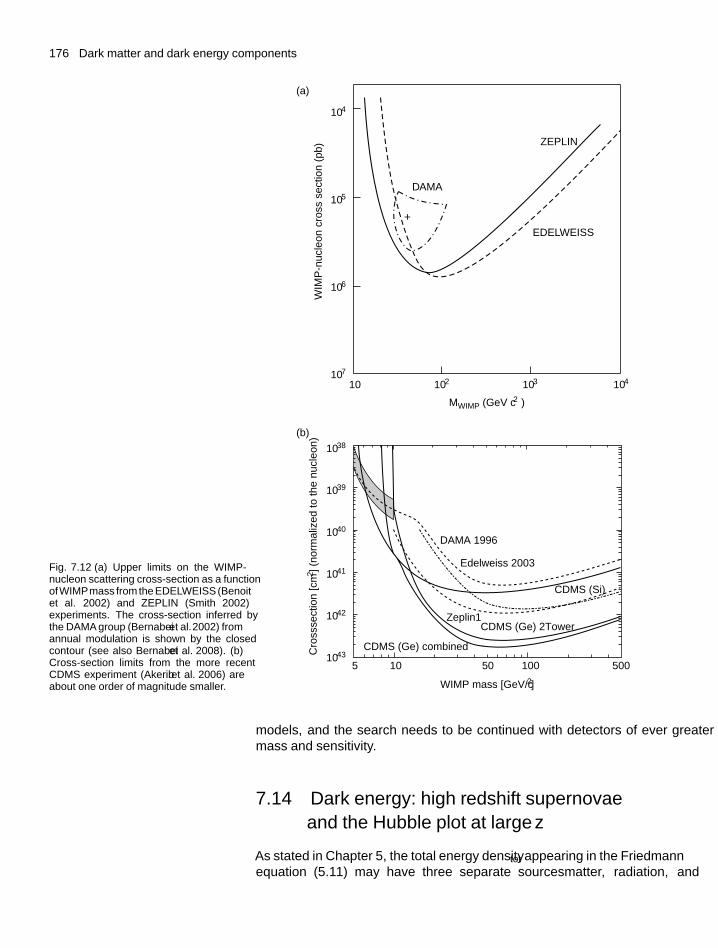
176 Dark matter and dark energy components
Fig. 7.12 (a) Upper limits on the WIMP-nucleon scattering cross-section as a functionofWIMPmass from the EDELWEISS (Benoitet al. 2002) and ZEPLIN (Smith 2002)experiments. The cross-section inferred bythe DAMA group (Bernabei et al. 2002) fromannual modulation is shown by the closedcontour (see also Bernabei et al. 2008). (b)Cross-section limits from the more recentCDMS experiment (Akerib et al. 2006) areabout one order of magnitude smaller.
Cro
ss–s
ectio
n [c
m2 ]
(nor
mal
ized
to th
e nu
cleo
n) 10–38
10–39
10–40
10–41
CDMS (Ge) combined
CDMS (Si)
CDMS (Ge) 2–TowerZeplin–1
DAMA 1996
Edelweiss 2003
5 10 50 100 500
WIMP mass [GeV/c2]
10–42
10–43
104102 10310
MWIMP (GeV c–2)
WIM
P-nu
cleo
n cr
oss
sect
ion
(pb)
+
DAMA
ZEPLIN
EDELWEISS
10–5
10–6
10–7
10–4
(a)
(b)
models, and the search needs to be continued with detectors of ever greatermass and sensitivity.
7.14 Dark energy: high redshift supernovaeand the Hubble plot at large z
As stated in Chapter 5, the total energy density ρtot appearing in the Friedmannequation (5.11) may have three separate sources—matter, radiation, and
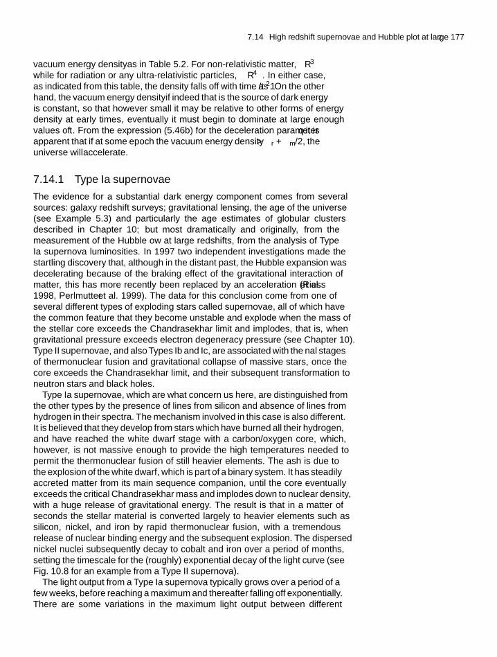
7.14 High redshift supernovae and Hubble plot at large z 177
vacuum energy density—as in Table 5.2. For non-relativistic matter, ρ ∝ R−3
while for radiation or any ultra-relativistic particles, ρ ∝ R−4. In either case,as indicated from this table, the density falls off with time as 1/t2. On the otherhand, the vacuum energy density—if indeed that is the source of dark energy—is constant, so that however small it may be relative to other forms of energydensity at early times, eventually it must begin to dominate at large enoughvalues of t. From the expression (5.46b) for the deceleration parameter q it isapparent that if at some epoch the vacuum energy density ρ� > ρr +ρm/2, theuniverse will accelerate.
7.14.1 Type Ia supernovae
The evidence for a substantial dark energy component comes from severalsources: galaxy redshift surveys; gravitational lensing, the age of the universe(see Example 5.3) and particularly the age estimates of globular clustersdescribed in Chapter 10; but most dramatically and originally, from themeasurement of the Hubble flow at large redshifts, from the analysis of TypeIa supernova luminosities. In 1997 two independent investigations made thestartling discovery that, although in the distant past, the Hubble expansion wasdecelerating because of the braking effect of the gravitational interaction ofmatter, this has more recently been replaced by an acceleration (Riess et al.1998, Perlmutter et al. 1999). The data for this conclusion come from one ofseveral different types of exploding stars called supernovae, all of which havethe common feature that they become unstable and explode when the mass ofthe stellar core exceeds the Chandrasekhar limit and implodes, that is, whengravitational pressure exceeds electron degeneracy pressure (see Chapter 10).Type II supernovae, and also Types Ib and Ic, are associated with the final stagesof thermonuclear fusion and gravitational collapse of massive stars, once thecore exceeds the Chandrasekhar limit, and their subsequent transformation toneutron stars and black holes.
Type Ia supernovae, which are what concern us here, are distinguished fromthe other types by the presence of lines from silicon and absence of lines fromhydrogen in their spectra. The mechanism involved in this case is also different.It is believed that they develop from stars which have burned all their hydrogen,and have reached the white dwarf stage with a carbon/oxygen core, which,however, is not massive enough to provide the high temperatures needed topermit the thermonuclear fusion of still heavier elements. The flash is due tothe explosion of the white dwarf, which is part of a binary system. It has steadilyaccreted matter from its main sequence companion, until the core eventuallyexceeds the critical Chandrasekhar mass and implodes down to nuclear density,with a huge release of gravitational energy. The result is that in a matter ofseconds the stellar material is converted largely to heavier elements such assilicon, nickel, and iron by rapid thermonuclear fusion, with a tremendousrelease of nuclear binding energy and the subsequent explosion. The dispersednickel nuclei subsequently decay to cobalt and iron over a period of months,setting the timescale for the (roughly) exponential decay of the light curve (seeFig. 10.8 for an example from a Type II supernova).
The light output from a Type Ia supernova typically grows over a period of afew weeks, before reaching a maximum and thereafter falling off exponentially.There are some variations in the maximum light output between different
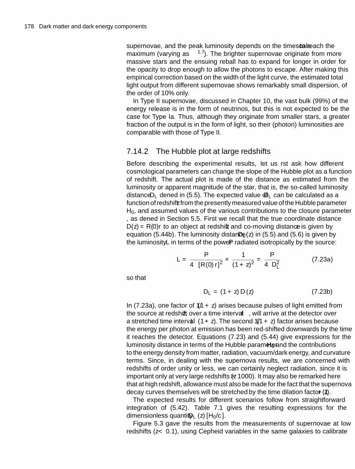
178 Dark matter and dark energy components
supernovae, and the peak luminosity depends on the timescale τ to reach themaximum (varying as ∼ τ1.7). The brighter supernovae originate from moremassive stars and the ensuing fireball has to expand for longer in order forthe opacity to drop enough to allow the photons to escape. After making thisempirical correction based on the ‘width’ of the light curve, the estimated totallight output from different supernovae shows remarkably small dispersion, ofthe order of 10% only.
In Type II supernovae, discussed in Chapter 10, the vast bulk (99%) of theenergy release is in the form of neutrinos, but this is not expected to be thecase for Type Ia. Thus, although they originate from smaller stars, a greaterfraction of the output is in the form of light, so their (photon) luminosities arecomparable with those of Type II.
7.14.2 The Hubble plot at large redshifts
Before describing the experimental results, let us first ask how differentcosmological parameters can change the slope of the Hubble plot as a functionof redshift. The actual plot is made of the distance as estimated from theluminosity or apparent magnitude of the star, that is, the so-called luminositydistance DL defined in (5.5). The expected value of DL can be calculated as afunction of redshift z from the presently measured value of the Hubble parameterH0, and assumed values of the various contributions to the closure parameter�, as defined in Section 5.5. First we recall that the true coordinate distanceD(z) = R(0)r to an object at redshift z and co-moving distance r is given byequation (5.44b). The luminosity distance DL(z) in (5.5) and (5.6) is given bythe luminosity L in terms of the power P radiated isotropically by the source:
L = P
4π [R (0) r]2× 1
(1 + z)2= P
4πD2L
(7.23a)
so that
DL = (1 + z) D (z) (7.23b)
In (7.23a), one factor of 1/(1 + z) arises because pulses of light emitted fromthe source at redshift z, over a time interval �t, will arrive at the detector overa stretched time interval �t(1 + z). The second 1/(1 + z) factor arises becausethe energy per photon at emission has been red-shifted downwards by the timeit reaches the detector. Equations (7.23) and (5.44) give expressions for theluminosity distance in terms of the Hubble parameter H0 and the contributionsto the energy density from matter, radiation, vacuum/dark energy, and curvatureterms. Since, in dealing with the supernova results, we are concerned withredshifts of order unity or less, we can certainly neglect radiation, since it isimportant only at very large redshifts (z > 1000). It may also be remarked herethat at high redshift, allowance must also be made for the fact that the supernovadecay curves themselves will be ‘stretched’ by the time dilation factor (1 + z).
The expected results for different scenarios follow from straightforwardintegration of (5.42). Table 7.1 gives the resulting expressions for thedimensionless quantity DL (z) [H0/c].
Figure 5.3 gave the results from the measurements of supernovae at lowredshifts (z < 0.1), using Cepheid variables in the same galaxies to calibrate
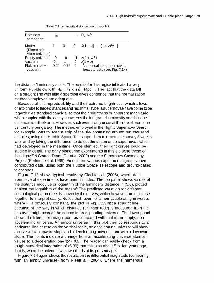
7.14 High redshift supernovae and Hubble plot at large z 179
Table 7.1 Luminosity distance versus redshift
Dominantcomponent
�m �� �k DLH0/c
Matter(Einstein–deSitter universe)
1 0 0 2(1 + z)[1 − (1 + z)−1/2]
Empty universe 0 0 1 z (1 + z/2)
Vacuum 0 1 0 z(1 + z)Flat, matter +
vacuum0.24 0.76 0 Numerical integration giving
best fit to data (see Fig. 7.14)
the distance/luminosity scale. The results for this region of z indicated a veryuniform Hubble flow with H0 = 72 km s−1 Mpc−1. The fact that the data fallon a straight line with little dispersion gives confidence that the normalizationmethods employed are adequate.
Because of this reproducibility and their extreme brightness, which allowsone to probe to large distances and redshifts, Type Ia supernovae have come to beregarded as ‘standard candles’, so that their brightness or apparent magnitude,when coupled with the decay curve, fixes the integrated luminosity and thus thedistance from the Earth. However, such events only occur at the rate of order oneper century per galaxy. The method employed in the High z Supernova Search,for example, was to scan a strip of the sky containing around ten thousandgalaxies, using the Hubble Space Telescope, then to repeat the survey 3 weekslater and by taking the difference, to detect the dozen or so supernovae whichhad developed in the meantime. Once identified, their light curves could bestudied in detail. The early pioneering experiments in this field were those ofthe High z SN Search Team (Riess et al. 2000) and the Supernova CosmologyProject (Perlmutter et al. 1999). Since then, various experimental groups havecontributed data, using both the Hubble Space Telescope and ground-basedtelescopes.
Figure 7.13 shows typical results by Clochiatti et al. (2006), where datafrom several experiments have been included. The top panel shows values ofthe distance modulus or logarithm of the luminosity distance in (5.6), plottedagainst the logarithm of the redshift z. The predicted variation for differentcosmological parameters is shown by the curves, which however, are too closetogether to interpret easily. Notice that, even for a non-accelerating universe,where H is obviously constant, the plot in Fig. 7.13 is not a straight line,because of the way in which distance (or magnitude) is measured from theobserved brightness of the source in an expanding universe. The lower panelshows the difference in magnitude, as compared with that in an empty, non-accelerating universe. An empty universe in this plot then corresponds to ahorizontal line at zero on the vertical scale, an accelerating universe will showa curve with an upward slope and a decelerating universe, one with a downwardslope. The points indicate a change from an accelerating universe at small zvalues to a decelerating one for z > 0.5. The reader can easily check from arough numerical integration of (5.39) that this was about 5 billion years ago,that is, when the universe was two-thirds of its present age.
Figure 7.14 again shows the results on the differential magnitude (comparingwith an empty universe) from Riess et al. (2004), where the numerous
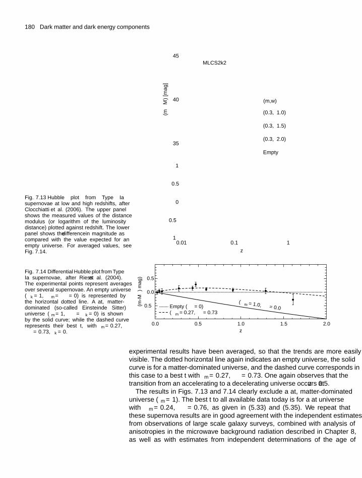
180 Dark matter and dark energy components
Fig. 7.13 Hubble plot from Type Iasupernovae at low and high redshifts, afterClocchiatti et al. (2006). The upper panelshows the measured values of the distancemodulus (or logarithm of the luminositydistance) plotted against redshift. The lowerpanel shows the difference in magnitude ascompared with the value expected for anempty universe. For averaged values, seeFig. 7.14.
45MLCS2k2
(�m,w)
(0.3, – 1.0)
(0.3, – 1.5)
(0.3, – 2.0)
Empty
40
(m–
M)
[mag
]
35
1
0.5
0
–0.5
–10.01 0.1
z
1
Fig. 7.14 Differential Hubble plot from TypeIa supernovae, after Riess et al. (2004).The experimental points represent averagesover several supernovae. An empty universe(�k = 1, �m = �� = 0) is represented bythe horizontal dotted line. A flat, matter-dominated (so-called Einstein–de Sitter)universe (�m = 1, �� = �k = 0) is shownby the solid curve; while the dashed curverepresents their best fit, with �m = 0.27,�� = 0.73, �k = 0.
0.5
0.5
Empty (�� = 0)(�m = 0.27, �� = 0.73
�(m
-M)
mag
)
(�m = 1.0, �� = 0.0
0.0
1.0z
1.5 2.00.0
–0.5
experimental results have been averaged, so that the trends are more easilyvisible. The dotted horizontal line again indicates an empty universe, the solidcurve is for a matter-dominated universe, and the dashed curve corresponds inthis case to a best fit with �m = 0.27, �� = 0.73. One again observes that thetransition from an accelerating to a decelerating universe occurs at z ∼ 0.5.
The results in Figs. 7.13 and 7.14 clearly exclude a flat, matter-dominateduniverse (�m = 1). The best fit to all available data today is for a flat universewith �m = 0.24, �� = 0.76, as given in (5.33) and (5.35). We repeat thatthese supernova results are in good agreement with the independent estimatesfrom observations of large scale galaxy surveys, combined with analysis ofanisotropies in the microwave background radiation described in Chapter 8,as well as with estimates from independent determinations of the age of
7.14 High redshift supernovae and Hubble plot at large z 181
the universe, for example, from globular clusters (see Example 5.3 andSection 10.3).
Example 7.3 In a flat universe, with �m(0) = 0.24 and ��(0) = 0.76, atwhat value of z will the acceleration/deceleration be zero?
From (5.46), q (z) = 12�m (0) (1 + z)3 − �� (0), which is zero when
(1 + z) = [2�� (0)/�m (0)]1/3, or z = 0.85, somewhat larger than the zvalue of the flat maximum in the dotted curve in Fig. 7.14. A universewhich is neither accelerating nor decelerating is often said to be ‘coasting’.
We should note here that the analyses described above involve a comparisonof high redshift with low redshift supernovae, so that the absolute luminosityscale, which is of course necessary in order to measure the Hubble parameter,is not required when comparing slopes. There are also potential complicationsin comparing the luminosities of supernovae at different redshifts, since theyoccur at different epochs and the metal content in early stars may be less thanthat in more recent ones, which have formed from the recycled debris of earlierstellar generations, and this could affect the opacity and hence the luminosity.This and other possible differential effects, such as dimming due to absorptionor scattering by dust, have been analysed by the various research groups inexhaustive detail, and shown to have only minor effects on the results.
7.14.3 Interpretation of the supernovae Ia results
As indicated in Chapter 5, the acceleration of the universe in recent times (z <
0.5) has been interpreted in terms of a vacuum energy term, which is time andz-independent, and identical with Einstein’s cosmological constant (see (5.23)).At present it is not at all clear that the dark energy is actually associated withsuch a vacuum state. For example, it could arise as the ‘latent heat’ as a resultof some sort of phase transition. Or the dark energy could be the manifestationof some new type of evolving scalar field, in so-called ‘quintessence’ models.More radical suggestions—so far with absolutely no supporting evidence—arethat the dark energy (or dark matter) terms have appeared artificially, because ofsubtle deviations from Newton’s inverse square law of gravitational attractionat very large, cosmological distances, as discussed in Section 2.10. In fact thereis compelling evidence for dark matter, shown above in Fig. 7.6, which is quiteindependent of assumptions about any possible deviations from the inversesquare law.
Assuming that the dark energy is not an artefact, the equation of statedescribing it may of course be different from that for the vacuum in Table 5.2,and the ratio of pressure to density could be time-dependent. From thesupernovae results, when combined with data from galaxy surveys and from theacoustic peak analysis of cosmic microwave background (CMB) fluctuationsdescribed in Chapter 8, it is possible to measure the quantity w = P/ρc2
occurring in the equation of state for the dark energy, but only by assumingthat it is time-independent. Then one finds as in (5.36)
wdarkenergy = −0.97 ± 0.08 (7.24)
consistent with the value w = − 1 for a simple vacuum/cosmological constant.
182 Dark matter and dark energy components
One of the major difficulties in identifying the dark energy with vacuumenergy arises when one considers its time evolution. For example, the ratio ofvacuum energy density to matter energy density today is ρ�/ρm ∼ 3, but whileρ� is constant, ρm ∝ R−3 ∝ (1 + z)3. Thus ρ�/ρm ∼ 3/(1 + z)3, and at the timeof decoupling of matter and radiation, when (1 + z) ∼ 1100, the ratio ρ�/ρm
would have been 10−9 only. Conversely, in the future the ratio will becomevery large, as the matter density falls off as 1/R3 and the scale parameter R willeventually increase exponentially with time.
Given this very large variation in the relative contribution of vacuum energyto the total closure parameter, a major puzzle is the fact that at the present epochit just happens to be within a factor 3 of the matter energy density. To circumventthis problem, one can postulate that the dark energy is associated with somenew type of scalar field—called quintessence—for which the equation of state issuch that the ratio w = P/ρc2 < −1/3 so as to ensure an accelerated expansion(see (5.46)), and is time dependent and of magnitude to reproduce the valuemeasured in (7.24) at modest z-values. The quintessence field can be arrangedto have an energy density which at early times closely follows or tracks (but isless than) the density of radiation, and after the era of matter–radiation equality,tracks the matter density. Referring to Table 5.2, it is noted that both radiationand matter energy densities vary as 1/t2, so that if the quintessence field hadthis property, its energy density would be a constant fraction of the total energydensity. Obviously small variations on the 1/t2 dependence are also possible,for not too complicated quintessence potentials.
Over the years, there have been many interesting suggestions regarding theorigin of dark energy. Could it be somehow related to a breakdown of Newtoniangravity at very short distances, reminiscent of the ‘curled up’ extra dimensionsin supergravity models? The magnitude of the dark energy density from �� is
ε = 4.1 GeV m−3,
and if we express this in natural units (h = c = 1), this density will correspondto a fundamental length given by
L4 = hc
ε,
where hc = 0.197 GeV fm has dimensions of energy × length, and ε hasdimensions of energy/(length)3. One thus finds a value for L of 84 μm.Unfortunately for this proposal, the inverse square law has in fact been found tobe valid using a very precise torsion balance, over the range from 9 mm downto 55 μm (Kapner et al. 2007).
7.15 Vacuum energy: the Casimir effect
In Chapter 5 we already mentioned that present observations, such as thosedescribed in the previous section, appear to require for their interpretation amajor contribution from dark vacuum energy to the present energy density ofthe universe. The vacuum energy itself is postulated to arise through quantumfluctuations, that is, the spontaneous appearance and disappearance of virtual
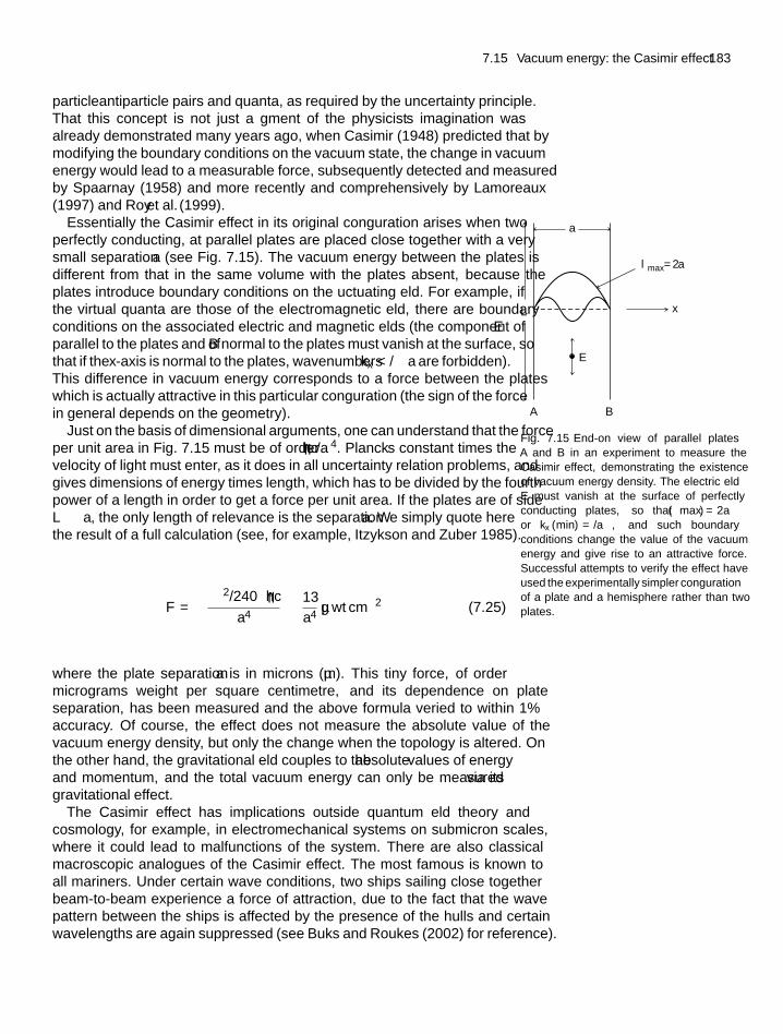
7.15 Vacuum energy: the Casimir effect 183
particle–antiparticle pairs and quanta, as required by the uncertainty principle.That this concept is not just a figment of the physicist’s imagination wasalready demonstrated many years ago, when Casimir (1948) predicted that bymodifying the boundary conditions on the vacuum state, the change in vacuumenergy would lead to a measurable force, subsequently detected and measuredby Spaarnay (1958) and more recently and comprehensively by Lamoreaux(1997) and Roy et al. (1999).
Essentially the Casimir effect in its original configuration arises when twoperfectly conducting, flat parallel plates are placed close together with a verysmall separation a (see Fig. 7.15). The vacuum energy between the plates isdifferent from that in the same volume with the plates absent, because theplates introduce boundary conditions on the fluctuating field. For example, ifthe virtual quanta are those of the electromagnetic field, there are boundaryconditions on the associated electric and magnetic fields (the component of Eparallel to the plates and of B normal to the plates must vanish at the surface, sothat if the x-axis is normal to the plates, wavenumbers kx < π/a are forbidden).This difference in vacuum energy corresponds to a force between the plateswhich is actually attractive in this particular configuration (the sign of the forcein general depends on the geometry).
L
a
E
A B
lmax = 2a
x
Fig. 7.15 End-on view of parallel platesA and B in an experiment to measure theCasimir effect, demonstrating the existenceof vacuum energy density. The electric fieldE must vanish at the surface of perfectlyconducting plates, so that λ(max) = 2aor kx (min) = π/a, and such boundaryconditions change the value of the vacuumenergy and give rise to an attractive force.Successful attempts to verify the effect haveused the experimentally simpler configurationof a plate and a hemisphere rather than twoplates.
Just on the basis of dimensional arguments, one can understand that the forceper unit area in Fig. 7.15 must be of order hc/a4. Planck’s constant times thevelocity of light must enter, as it does in all uncertainty relation problems, andgives dimensions of energy times length, which has to be divided by the fourthpower of a length in order to get a force per unit area. If the plates are of sideL � a, the only length of relevance is the separation a. We simply quote herethe result of a full calculation (see, for example, Itzykson and Zuber 1985).
F = −(π2/240
)hc
a4∼ 13
a4μg wt cm−2 (7.25)
where the plate separation a is in microns (μm). This tiny force, of ordermicrograms weight per square centimetre, and its dependence on plateseparation, has been measured and the above formula verified to within 1%accuracy. Of course, the effect does not measure the absolute value of thevacuum energy density, but only the change when the topology is altered. Onthe other hand, the gravitational field couples to the absolute values of energyand momentum, and the total vacuum energy can only be measured via itsgravitational effect.
The Casimir effect has implications outside quantum field theory andcosmology, for example, in electromechanical systems on submicron scales,where it could lead to malfunctions of the system. There are also classicalmacroscopic analogues of the Casimir effect. The most famous is known toall mariners. Under certain wave conditions, two ships sailing close togetherbeam-to-beam experience a force of attraction, due to the fact that the wavepattern between the ships is affected by the presence of the hulls and certainwavelengths are again suppressed (see Buks and Roukes (2002) for reference).
184 Dark matter and dark energy components
7.16 Problems with the cosmological constantand dark energy
The cosmological constant � = 8πG ρvac presents one of the major—if notthe major—conceptual problems in cosmology, and has done so ever sinceEinstein introduced it. It has long been argued that the dark energy densityassociated with the cosmological constant ought to have a ‘natural’ valuedetermined by the scale of gravity. This natural unit is then the Planck mass
energy MPLc2 = (hc5/G)1/2 = 1.2 × 10¹⁹ GeV, in a cube of side equal to the
Planck length h/MPLc (see (1.12)), that is, an energy density
(MPLc2
)4(hc)3
∼ 10123 GeV m−3 (7.26)
a truly gigantic number, which of course is nonsensical since it would implythat the universe could only be a few seconds old at most. So, it is perhapsinstructive to see in more detail how this number is arrived at.
In quantum field theory one can describe the vacuum fluctuations of theboson fields as due to an ensemble of simple harmonic oscillators of differentfrequencies. The energy of one such (bosonic) oscillator is (n + 1/2) hω whereω is an angular frequency and n = 0, 1, 2, . . .. The vacuum or ground state hasthe so-called ‘zero-point energy’ E = 1
2 hω. In a sense, it is a matter of choicewhether one takes this zero-point energy seriously or simply ignores it, sincemeasurements are usually about energy differences, and only when we cometo gravity do we have to worry about the absolute energy value. However, ifwe try to identify it with the mysterious, dark vacuum energy, then we haveto sum over all oscillators in the volume. From (1.16), the number of possiblequantum states in a spatial volume V , with wave numbers k = p/h lying in theelement k → k +dk and integrated over all directions, is 4πV k2 dk/(2π)3. Sothe total energy per unit volume of all the oscillators will be
ε = E
V=[
h(4π2)]×
∫k2dk ωk (7.27)
The angular frequency is related to the wavenumber by ω2k = k2c2 + m2c4/h2
where m is the oscillator mass. Obviously this integral is divergent, but let uscut it off at some value km or Em � mc2. Then, with ωk ≈ kc in the relativisticapproximation
ε =(
hc
16π2
)k4
m = E4m[
16π2 (hc)3] (7.28)
Here, the cut-off is arbitrary. For example, we can place it at an energy scalewhere we expect quantum field theory to start to fail, and that is the Planck scaleEm = MPL of quantum gravity. Another excuse for choosing this scale is that itis the ‘natural’ scale of energy from combining the fundamental constants G, h,and c, that is, (hc/G)1/2. Including the numerical constants left out in (7.26),
7.16 Problems with cosmological constant and dark energy 185
this gives ε ∼ 10121 GeV m−3 as before, to be compared with the critical energydensity in (5.26) of ρc ∼ 5 GeV m−3, of which only a part can be assigned asvacuum energy. So why is the observed vacuum energy/cosmological constantonly about 10−121 of the naïve expectation?
Of course, one might vary the value of Em so that the vacuum energy densityis of the same order as the critical density, that is, ε = ρc = 5 GeV m−3. Thensubstituting in (7.28) would give Em ∼ 0.01 eV only. This is ridiculously smallin comparison with the masses of practically all known elementary particles, oreven of atomic energy levels. It has been remarked, however, that this energyis indeed comparable with mass differences of light neutrinos (4.12). It wouldindeed be extraordinary if the acceleration of the universe were somehow tiedup with neutrino masses, but the mystery of dark energy is such that even themost outlandish ideas cannot be ignored.
Twenty-five years ago, before the importance of dark energy was fullyapparent, it was believed that the matter density was such that �m ∼ �tot ∼ 1and that the cosmological constant might even be identically zero, and darkmatter made up the vast bulk of the energy density. In view of the aboveargument, the difficulty then was to understand why the cosmological constantwas so incredibly small, or even zero. Here, at least one can say that zerois a natural number, for which a reason might be found. For example, themasslessness of the photon is associated with a symmetry principle, namelythe local gauge invariance of the electromagnetic interaction as described inSection 3.7. However, no symmetry principle is known that could set � = 0.Indeed, the finiteness of the vacuum energy/cosmological constant seems tofollow inexorably from quantum mechanics, for the very simple reason thatthe virtual states of the real particles which contribute to �m must contributeto ��.
However, the above integral will include the summed effects of all types ofelementary field, with somewhat different amplitudes and phases, and there canbe cancellations. For example, the energy of a fermion oscillator, analogous tothe above expression for a boson oscillator, is (n − 1/2) hω, so that the zero-point energy comes in with the opposite sign. (This comes about because thewave functions describing creation and annihilation of bosons and fermionsobey commutation and anti-commutation relations respectively.) So in a theoryof exact supersymmetry, where every boson is matched by a fermion of thesame mass and vice-versa, there would indeed be complete cancellations, witha vacuum energy of zero. However, we know that in the real world, even ifsupersymmetry turns out to be valid, it must be a badly broken symmetry. Whileat very large values of k in (7.27), well above the supersymmetric scale, therecould be exact cancellations, this would not be the case at lower k values.
The actual situation is of course somewhat worse than this, since thesupernovae results present us with a finite, non-zero number for the dark energydensity, inconceivably small in comparison with what might be expected, butone for which the relative contribution to the overall energy density apparentlychanges with time. Attempts to model this behaviour have been described inthe previous section.
Finally, a different approach to the problem has been to appeal to the anthropicprinciple, namely that life exists only when the laws of physics allow it. In thiscase, it is the value for � at the present epoch. Had it differed by just an orderof magnitude or so, there would have been no human race to ponder on the
186 Dark matter and dark energy components
problem. As the saying goes, we live in the best of all possible worlds. Thisargument perhaps becomes more plausible in the context of inflationary modelsof the early universe, described in Chapter 8. These suggest that our particularuniverse is just one of an enormous number of parallel universes, so that thehuman race could have evolved in the one where conditions happened to suit it.
In summary, the phenomenon of the cosmological constant or dark energy,accounting at the present time we believe for the bulk of the energy in theuniverse, is simply not understood, and this, like our incomprehension ofthe matter–antimatter asymmetry of the universe, could be ranked as a majorfailure in the subjects of cosmology and particle physics. These failures havenot grown up overnight. The problems of dark matter and of the vacuumenergy/cosmological constant have been lurking for at least 70 years, but theyhave become more acute in the last two decades because of the vastly improvedquality and quantity of the experimental data, and the remarkable discovery ofan accelerating universe. However, it cannot be too strongly emphasized that itis precisely such problems which keep the subject of particle astrophysics aliveand stimulating and full of great challenges for the future.
7.17 Summary
• The rotation curves of stars in spiral galaxies imply that the bulk of thematter (80–90%) is non-luminous, and located in a galactic halo.
• Studies of X-rays from galactic clusters indicates velocities of the gasparticles emitting the X-rays which are far in excess of escape velocitiesbased on the visible mass.
• Dark matter is also required in cosmological models of the early universe,if the structure of galaxies and galaxy clusters is to evolve from the verysmall primordial density fluctuations deduced from inhomogeneities inthe microwave radiation (discussed in Chapter 5).
• Independent evidence for dark matter is found from the gravitationallensing of distant galaxies and clusters by foreground galaxies.Gravitational microlensing of individual stars, appearing as a temporary,achromatic enhancement in luminosity, shows that some of the galacticdark matter is baryonic, this matter appearing in the form of so-calledMACHOs, which are dark star-like objects with masses of 0.001 − 0.1solar masses.
• Baryonic dark matter makes less than 25% contribution to the total darkmatter density, and the bulk of dark matter is non-baryonic.
• The most likely candidates for dark matter are WIMPs, that is, verymassive, weakly interacting particles, constituting ‘cold’ dark matter.Until the nature of such particles is established, the most commonsuggestion is that they are supersymmetric particles such as neutralinos.
• Several experiments are under way to detect WIMPs directly byobserving nuclear recoils from elastic scattering of WIMPs, so far withno success.
• Observations of Type Ia supernovae at high redshifts (z ∼ 1) suggest thatin earlier times the expansion rate (i.e. the Hubble parameter H ) was lessthan it is today; or that, relative to earlier times, the universal expansionis now accelerating.
Problems 187
• The present acceleration is interpreted in terms of a finite value for thecosmological constant, or for the existence of dark (vacuum) energy. Thisdark energy seems to account for some 2/3 of the total energy density ofthe universe today.
• The reality of vacuum energy is evidenced by the laboratory observationof the Casimir effect, which is a manifestation of a change in the vacuumenergy when boundary conditions are imposed on it.
• There is no satisfactory explanation for the observed magnitude of thedark energy, which at the present time is comparable in magnitude withthe matter energy density. If the dark energy is identified with vacuumenergy, then in times past it would have been negligible while in the futureit will become dominant. Other possible sources of dark energy have beenproposed, involving completely new types of interaction. However, thepuzzle of the present magnitude of the dark energy remains.
Problems
More challenging or longer questions are denoted by an asterisk.
(7.1) Estimate the angular deflection of a photon by a pointmass M , according to Newtonian mechanics. Expressthe result in terms of b, the closest distance of approach.
(7.2) Calculate an expression for the tangential velocity v of astar near the edge of the disc of a spiral galaxy of radius Rand mass M , and thus find an expression for the opticaldepth τ for microlensing in terms of v. Give numbers forthe Milky Way, with a mass of 1.5 ×10¹¹ solar massesand a disc radius of 15 kpc.
(7.3) Obtain an expression for the kinetic energy ER of anucleus of mass MR recoiling in an elastic collisionwith a dark matter particle of mass MD and incidentkinetic energy ED, in terms of the angle of emissionrelative to the incident direction. Find the limiting valuesof recoil energy in terms of MD and MR. Calculatethe maximum recoil energy of a nucleus of 80 proton
masses, in collision with a dark matter particle of mass1000 times the proton mass, travelling with a typicalgalactic velocity of 200 km s−1.
(7.4) Assume that the universe is flat, with �m(0) = 0.24,��(0) = 0.76. What is the numericalvalue of theacceleration or deceleration with respect to the Earth,of a galaxy at redshift z = 0.03? Compare this with thelocal acceleration (g) due to the Earth’s gravity. Neglectthe ‘peculiar velocity’ of the Earth with respect to theHubble flow and assume H0 = 70 km s−1 Mpc−1.
(7.5) Show that, if the vacuum energy density and matterenergy density today are comparable in magnitude, thenwhen the universe was a fraction f of its present age, therelative contribution of the vacuum energy would havebeen f 2.
(7.6) Verify the results given in Table 7.1 for luminositydistances as a function of redshift.
8Development ofstructure in theearly universe
8.1 Preamble
The Big Bang model described in Chapter 5 seems to give a rather convincingdescription of the development of the early universe. It is underpinned by threestriking phenomena:
• The observation of the redshift of distant galaxies.• The correct prediction of the abundances of the light elements via
primordial nucleosynthesis.• The existence of the all-pervading cosmic microwave background (CMB)
radiation.
This success is all the more remarkable since the principal tenets of the model—isotropy and homogeneity of the ‘cosmic fluid’—are to be contrasted with theuniverse today, characterized by a decidedly non-isotropic, non-homogeneousnature—galaxies, galactic clusters, voids, and so forth. The question arises:how did we get from the uniformity of the Big Bang model to the presentuniverse with its lumpy structure?
As described in the following pages, it can plausibly be argued that thisstructure had its origins in quantum fluctuations in energy density whichoccurred in the very early universe and were then ‘frozen-out’when the universeunderwent an exponential and superluminal expansion stage called inflation.These tiny fluctuations in density and temperature—typically at the 10−5
level—then acted as seeds for the development of much greater fluctuationsin density via the subsequent process of gravitational collapse during the epochof matter domination.
In Section 8.3 we outline the inflation scenario, which was postulated overtwo decades ago in response to some difficulties with the Big Bang model,mainly with respect to the initial conditions which are apparently required.Later in the chapter we touch on the subject of galaxy formation. One of themost remarkable features of the universe is that stars are always clumped intogalaxies each containing of order 1011 stars. The galaxies are separated bydistances some two orders of magnitude larger than their diameters (∼ Mpcas compared with ∼ 10 kpc), and one might ask the question; why has matterbecome distributed in this particular fashion—rather than, for example, in onegiant galaxy? To anticipate our discussion, the present answer appears to bethat in the early universe primordial density fluctuations could only start togrow, provided that they were spread out over distances which now correspondto the dimensions of galaxy clusters, and that these dimensions were in turn
8.2 Galactic and intergalactic magnetic fields 189
determined by the properties and interactions of the primordial photons andneutrinos which dominated the radiation era.
In this text, we do not enter into the very complex cosmology of thedistribution and formation of galaxies, but only discuss in general terms howthe universe could have progressed from the uniformity of the Big Bang modelto the very lumpy structure of the universe today.
8.2 Galactic and intergalactic magnetic fields
In this section we discuss very briefly the nature and magnitude of theintergalactic magnetic fields, to try to assess whether they were important inthe early development of the universe. Inside our own galaxy, the interstellarmagnetic fields are very significant and follow the spiral arms. The averagevalue of this galactic field B ∼ 3μG (0.3 nT) and its energy density is thereforeB2/8π ∼ 0.2 eV cm−3, so is comparable with the energy density of cosmicmicrowave radiation (0.26 eV cm−3) and that of the cosmic rays in deep space(∼1 eV cm−3). This galactic field has been measured, for example, by observingthe Faraday rotation of polarized light from pulsars (Han et al. 2006). Therotation is proportional to the line integral of the B-field and the square of thewavelength, so the mean field can be found from the wavelength dependenceof the rotation, and varies from about 2 × 10⁻⁶ G in outer parts of the spiralarms to 4 × 10⁻⁶ G towards the central hub.
The intergalactic field is known only within limits and is certainly very muchless than that inside the galaxy. Magnetic fields associated with galaxy andcluster filaments, that is, on the scale of 1 Mpc or less, have been estimatedfrom the soft synchrotron radiation emitted by electrons traversing the field,and are of order 10−7 G or less (Kronberg 2004). For very deep space (i.e.distances of order 10–100 Mpc), a value of 10−11 G is indicated from theobservation in the AUGER experiment (see Section 9.13) that extensive airshowers produced by protons of energy above 6 × 10¹⁹eV are correlated (withinabout 30) with known point sources (active galactic nuclei, AGNs) up to 75Mpc distant (Dermer 2007).
Some models postulate that very weak and diffuse intergalactic fields areproduced by the passage of high-energy charged particles—cosmic rays—produced as ejecta and jets from supernova explosions, that is, following the eraof star formation (roughly, for redshifts z < 12). Another view is that the fieldscould have been generated by dynamic amplification of weaker ‘seed’ fieldsgenerated much earlier, in the primordial proton–electron plasma before theera of recombination (i.e. for z > 1100). The density fluctuations in the plasmawould produce ‘winds’ of photons streaming from high to low density regions.The idea is that such photons would interact to separate the lighter electronsfrom the heavier protons, giving rise to charge separation and rotating electriccurrents seeding primordial magnetic fields.
However, since the present intergalactic field appears to be less than 10−5
of the galactic field, it seems unlikely that magnetic fields could have playeda very significant role in the development of structure on very large (clusterand supercluster) scales. We shall follow the conventional wisdom, whichtreats gravity as the main player in these developments, with electromagneticinteractions in a subsidiary role.
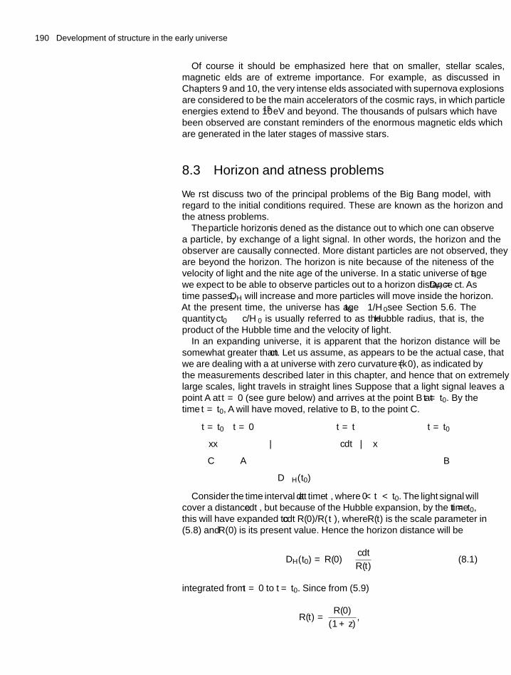
190 Development of structure in the early universe
Of course it should be emphasized here that on smaller, stellar scales,magnetic fields are of extreme importance. For example, as discussed inChapters 9 and 10, the very intense fields associated with supernova explosionsare considered to be the main accelerators of the cosmic rays, in which particleenergies extend to 1015 eV and beyond. The thousands of pulsars which havebeen observed are constant reminders of the enormous magnetic fields whichare generated in the later stages of massive stars.
8.3 Horizon and flatness problems
We first discuss two of the principal problems of the Big Bang model, withregard to the initial conditions required. These are known as the horizon andthe flatness problems.
The particle horizon is defined as the distance out to which one can observea particle, by exchange of a light signal. In other words, the horizon and theobserver are causally connected. More distant particles are not observed, theyare beyond the horizon. The horizon is finite because of the finiteness of thevelocity of light and the finite age of the universe. In a static universe of age t,we expect to be able to observe particles out to a horizon distance DH = ct. Astime passes, DH will increase and more particles will move inside the horizon.At the present time, the universe has age t0 ∼ 1/H0—see Section 5.6. Thequantity ct0 ∼ c/H0 is usually referred to as the Hubble radius, that is, theproduct of the Hubble time and the velocity of light.
In an expanding universe, it is apparent that the horizon distance will besomewhat greater than ct. Let us assume, as appears to be the actual case, thatwe are dealing with a flat universe with zero curvature (k = 0), as indicated bythe measurements described later in this chapter, and hence that on extremelylarge scales, light travels in straight lines Suppose that a light signal leaves apoint A at t = 0 (see figure below) and arrives at the point B at t = t0. By thetime t = t0, A will have moved, relative to B, to the point C.
t = t0 t = 0 t = t′ t = t0
x———x−−−−−→————–| ← cdt′ → |———————–x
C A B
←−−−−−−−−−−−−−DH(t0)−−−−−−−−−−−−−−−−−−−−−−−−−→Consider the time interval dt′at time t′, where 0 < t′ < t0. The light signal will
cover a distance cdt′, but because of the Hubble expansion, by the time t = t0,this will have expanded to cdt′R(0)/R(t′), where R(t) is the scale parameter in(5.8) and R(0) is its present value. Hence the horizon distance will be
DH(t0) = R(0)
∫cdt
R(t)(8.1)
integrated from t = 0 to t = t0. Since from (5.9)
R(t) = R(0)
(1 + z),
8.3 Horizon and flatness problems 191
then
dt = dz
[(1+z) H ],
so thatR(0)cdt
R(t)= cdz
H(8.2)
Therefore the horizon distance today, expressed in terms of the redshift z is
DH(t0) = c∫
dz
H(8.3)
where from (5.37)
H = H0
[�m(0)(1 + z)3 + �r(0)(1 + z)4 + ��(0) + �k(0)(1 + z)2
]1/2
The fraction of the universe, of current dimension R(0), which is inside theoptical horizon today is therefore proportional to
F = DH(t0)
R(0)=[
c
H0R(0)
]×∫
dz[�m(0) (1 + z)3 + �r(0) (1 + z)4 + ��(0) + �k(0)(1 + z)2
]1/2
(8.4)
integrated from z = 0 to z = ∞. We see from the integrand that if the lowerlimit of the integral is taken as z*, then for a matter-dominated universe, Fdecreases as 1/
√(1 + z∗) or t1/3, while it falls off as 1/(1 + z∗) or t1/2 in
the case of radiation dominance (see Table 5.2). Thus at early times or large zvalues, the fraction of the universe inside the horizon was much smaller than itis now.
This result also follows more briefly by observing that for most cosmologicalmodels, R(t) ∝ tn where n < 1, so that integrating from t = 0 to t = t0 theabove formula gives
DH(t0) = ct0(1 − n)
(8.5)
One observes that the ratio
DH(t)
R(t)∝ t(1−n) (8.6)
so that since n < 1, again the fraction of the universe which is causallyconnected was once much smaller than it is now.
Example 8.1 Calculate the particle horizon distance for a flat universedominated by (a) matter and (b) radiation.
Refer to Table 5.2. For a matter-dominated universe n = 2/3 and henceDH = 3ct0 = 2c/H0; while for the case of radiation domination, n = 1/2and DH = 2ct0 = c/H0, where we have used the fact that the ages forthe matter- and radiation-dominated cases are t0 = 2/(3H0) and 1/(2H0)
respectively. With 1/H0 = 14 Gyr, the corresponding horizon distances are2.5 × 1026 and 1.25 × 1026 m respectively.
192 Development of structure in the early universe
In particular, the time of decoupling of matter and radiation was tdec =4 × 10⁵ years (see Section (5.12)), and the horizon size then would have beenapproximately ctdec. By now, this would have expanded to ctdec(1+zdec) wherefrom (5.75) zdec = 1100. Hence, the angle subtended by that horizon distanceat the Earth today for the case of a flat, matter-dominated universe would be,with t0 = 1.4 × 10¹⁰ years
θdec ∼ ctdec (1 + zdec)
2c (t0 − tdec)∼ 1◦ (8.7)
This formula shows that only the microwave radiation observed over smallangular scales, of order one degree or so, corresponding to the time of thelast interaction of these photons, could ever have been causally connected andin thermal equilibrium with other matter. On the contrary, after allowing fora dipole anisotropy associated with the ‘peculiar velocity’ of the Earth withrespect to the microwave radiation, the temperature of the radiation is found tobe uniform to within one part in 105, out to the very largest angular scales. Thisis the horizon problem.
The flatness problem arises as follows. From (5.26) and (5.27) the fractionaldifference between the actual density and the critical density is
�ρ
ρ= (ρ − ρc)
ρ= 3kc2
8πGR2 ρ(8.8)
During the radiation-dominated era, ρ ∝ R−4. From (8.8) it follows that�ρ/ρ ∝ R2 ∝ t. So at early times, �ρ/ρ must have been much smallerthan it is today, when t ∼ 4 × 10¹⁷ s and it is of order unity. For example, for kT∼ 1014 GeV, a typical energy scale of grand unification, t ∼ 10−34 s, and at thattime �ρ/ρ would have been ∼ 10−34/1018 ∼ 10−52 (and even smaller thanthis if we include the period of matter dominance). How then could � = ρ/ρc
have been so closely tuned as to give of the order of unity today?In short, these two problems require a mechanism which allows thermal
equilibrium outside conventional particle horizons, and can reduce thecurvature k/R2 in (8.8) by a huge factor. A possible answer—indeed, the onlyone we have—was supplied by Guth in 1981 (who was actually concerned toreduce the possible monopole flux—see below). He postulated an extremelyrapid exponential expansion by a huge factor as a preliminary stage of the BigBang, a phenomenon known as inflation. Since that time, there have been anumber of inflationary models—old inflation, new inflation, chaotic inflation,eternal inflation, and so on—none of them yet fully capable of a completelysatisfactory description. However, there seems to be little doubt that some sort ofinflationary scenario is an obligatory first stage of the birth pangs of the universe.
8.4 Inflation
In this section we give a brief and qualitative description of the inflationscenario. First we recall the Friedmann equation (5.11)(
R
R
)2
= 8πG (ρ + ρ�)
3− kc2
R2
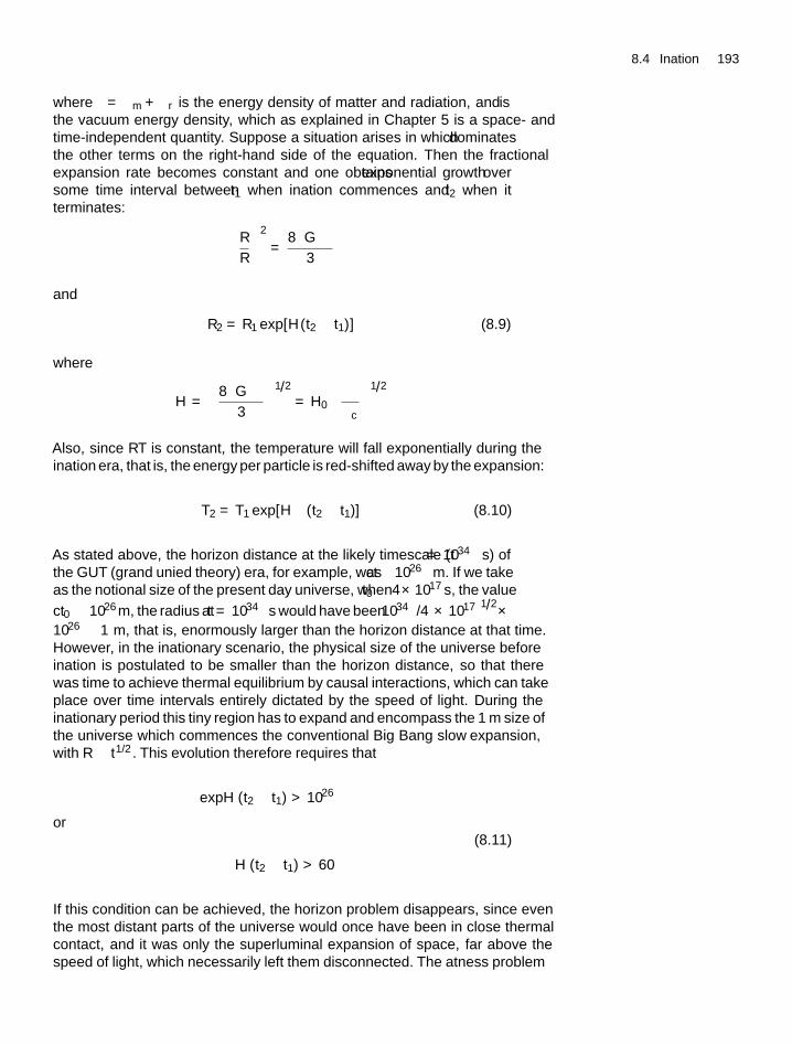
8.4 Inflation 193
where ρ = ρm + ρr is the energy density of matter and radiation, and ρ� isthe vacuum energy density, which as explained in Chapter 5 is a space- andtime-independent quantity. Suppose a situation arises in which ρ� dominatesthe other terms on the right-hand side of the equation. Then the fractionalexpansion rate becomes constant and one obtains exponential growth oversome time interval between t1 when inflation commences and t2 when itterminates: (
R
R
)2
= 8πGρ�
3
and
R2 = R1 exp [H (t2 − t1)] (8.9)
where
H =(
8πGρ�
3
)1/2
= H0
(ρ�
ρc
)1/2
Also, since RT is constant, the temperature will fall exponentially during theinflation era, that is, the energy per particle is red-shifted away by the expansion:
T2 = T1 exp [−H (t2 − t1)] (8.10)
As stated above, the horizon distance at the likely timescale (t = 10−34 s) ofthe GUT (grand unified theory) era, for example, was ct ∼ 10−26 m. If we takeas the notional size of the present day universe, when t0 ∼ 4×10¹⁷ s, the value
ct0 ∼ 1026 m, the radius at t = 10−34 s would have been(10−34/4 × 1017
)1/2×1026 ∼ 1 m, that is, enormously larger than the horizon distance at that time.However, in the inflationary scenario, the physical size of the universe beforeinflation is postulated to be smaller than the horizon distance, so that therewas time to achieve thermal equilibrium by causal interactions, which can takeplace over time intervals entirely dictated by the speed of light. During theinflationary period this tiny region has to expand and encompass the 1 m size ofthe universe which commences the conventional Big Bang ‘slow’ expansion,with R ∝ t1/2. This evolution therefore requires that
exp H (t2 − t1) > 1026
or(8.11)
H (t2 − t1) > 60
If this condition can be achieved, the horizon problem disappears, since eventhe most distant parts of the universe would once have been in close thermalcontact, and it was only the superluminal expansion of space, far above thespeed of light, which necessarily left them disconnected. The flatness problem
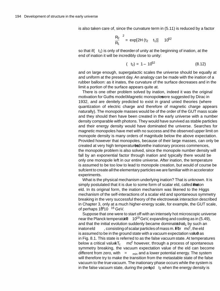
194 Development of structure in the early universe
is also taken care of, since the curvature term in (5.11) is reduced by a factor(R2
R1
)2
= exp [2H (t2 − t1)] ∼ 1052
so that if �(t1) is only of the order of unity at the beginning of inflation, at theend of inflation it will be incredibly close to unity:
�(t2) = 1 ± 10−52 (8.12)
and on large enough, supergalactic scales the universe should be equally flatand uniform at the present day. An analogy can be made with the inflation of arubber balloon: as it inflates, the curvature of the surface decreases and in thelimit a portion of the surface appears quite flat.
There is one other problem solved by inflation, indeed it was the originalmotivation for Guth’s model. Magnetic monopoles were suggested by Dirac in1932, and are definitely predicted to exist in grand unified theories (wherequantization of electric charge and therefore of magnetic charge appearsnaturally). The monopole masses would be of the order of the GUT mass scaleand they should then have been created in the early universe with a numberdensity comparable with photons. They would have survived as stable particlesand their energy density would have dominated the universe. Searches formagnetic monopoles have met with no success and the observed upper limit onmonopole density is many orders of magnitude below the above expectation.Provided however that monopoles, because of their large masses, can only becreated at very high temperatures, before the inflationary process commences,the monopole problem is also solved, since the monopole number density willfall by an exponential factor through inflation and typically there would beonly one monopole left in our entire universe. After inflation, the temperatureis assumed to be too low to lead to monopole creation, but would of course besufficient to create all the elementary particles we are familiar with in acceleratorexperiments.
What is the physical mechanism underlying inflation? That is unknown. It issimply postulated that it is due to some form of scalar field, called the inflatonfield. In its original form, the inflation mechanism was likened to the Higgsmechanism of the self-interactions of a scalar field and spontaneous symmetrybreaking in the very successful theory of the electroweak interaction describedin Chapter 3, only at a much higher-energy scale, for example, the GUT scale,of perhaps 1014−1016 GeV.
Suppose that one were to start off with an intensely hot microscopic universenear the Planck temperature kT ∼ 1019 GeV, expanding and cooling as in (5.49),and that the initial evolution suddenly became dominated at t = t1 by such an‘inflaton’fieldφ, consisting of scalar particles of mass m. For kT�mc2, the fieldis assumed to be in the ground state with a vacuum expectation value 〈φ〉 = 0 asin Fig. 8.1. This state is referred to as the ‘false vacuum’ state. At temperaturesbelow a critical value kTc ∼ mc2 however, through a process of spontaneoussymmetry breaking, the vacuum expectation value of the field can becomedifferent from zero, with 〈φ〉 = φmin and a lower potential energy. The systemwill therefore try to make the transition from the metastable state of the ‘false’vacuum to the ‘true’ vacuum. The inflationary phase occurs while the system isin the false vacuum state, during the period t1 → t2 when the energy density is
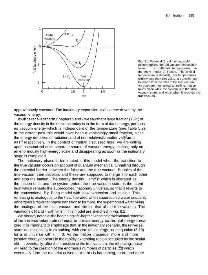
8.4 Inflation 195
0 0.5 1.0
T Tc>>
T Tc<<
Tc
T = T0 Truevacuum
Falsevacuum
�min �
V(�
) (a
rbitr
ary
units
)
–1
–2
0
1
Fig. 8.1 Potential V (φ) of the ‘inflaton’ fieldplotted against the field vacuum expectationvalue 〈φ〉 at different temperatures, inthe early model of inflation. The criticaltemperature is denoted Tc. For temperaturesslightly less than this value, a transition canbe made from the ‘false’ to the ‘true’ vacuumvia quantum-mechanical tunnelling. Inflationtakes place while the system is in the ‘false’vacuum state, and ends when it reaches the‘true’ vacuum.
approximately constant. The inflationary expansion is of course driven by thevacuum energy.
It will be recalled that in Chapters 5 and 7 we saw that a large fraction (75%) ofthe energy density in the universe today is in the form of dark energy, perhapsas vacuum energy which is independent of the temperature (see Table 5.2).In the distant past this would have been a vanishingly small fraction, sincethe energy densities of radiation and of non-relativistic matter vary as T 4 andas T 3 respectively. In the context of inflation discussed here, we are callingupon a second and quite separate source of vacuum energy, existing only onan enormously high-energy scale and disappearing as soon as the inflationarystage is completed.
The inflationary phase is terminated in this model when the transition tothe true vacuum occurs on account of quantum mechanical tunnelling throughthe potential barrier between the false and the true vacuum. ‘Bubbles’ of thetrue vacuum then develop, and these are supposed to merge into each otherand stop the inflation. The energy density ρ ∼ (mc2)4 which is liberated asthe inflation ends and the system enters the true vacuum state, is the ‘latentheat’ which reheats the supercooled inflationary universe, so that it reverts tothe conventional Big Bang model with ‘slow’ expansion and cooling. Thisreheating is analogous to the heat liberated when supercooled water suddenlyundergoes a first-order phase transition to form ice, the supercooled water beingthe analogue of the false vacuum and the ice that of the true vacuum. Thevariations of R and T with time in this model are sketched in Fig. 8.2.
We already noted at the beginning of Chapter 5 that the gravitational potentialof the universe today is almost equal to its mass energy, so the total energy is nearzero. It is important to emphasize that, in the inflationary scenario, the universestarts out essentially from nothing, with zero total energy, as in equation (5.13)for a flat universe with k = 0. As the inflation proceeds, more and morepositive energy appears in the rapidly expanding region occupied by the scalarfield φ: eventually, after the transition to the true vacuum, the ‘reheating’ phasewill lead to the creation of the enormous numbers of particles (∼1088!) whicheventually form the material universe. As this is happening, more and more
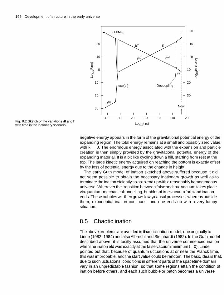
196 Development of structure in the early universe
Fig. 8.2 Sketch of the variations of R and Twith time in the inflationary scenario.
0
–10–20–30– 40
exp(�t )
kT = MPL
kT R
Decoupling
Now
Log
10R
(m)
Log
10kT
(GeV
)
Log10 t (s)
t1/2
t1/2 t –1/2
0 10 20
20
10
0
–10
–20
–30
20
10
–10
–20
–30
t –2/3
negative energy appears in the form of the gravitational potential energy of theexpanding region. The total energy remains at a small and possibly zero value,with k ≈ 0. The enormous energy associated with the expansion and particlecreation is then simply provided by the gravitational potential energy of theexpanding material. It is a bit like cycling down a hill, starting from rest at thetop. The large kinetic energy acquired on reaching the bottom is exactly offsetby the loss of potential energy due to the change in height.
The early Guth model of inflation sketched above suffered because it didnot seem possible to obtain the necessary inflationary growth as well as toterminate the inflation efficiently so as to end up with a reasonably homogeneousuniverse. Wherever the transition between ‘false’and ‘true’vacuum takes placevia quantum-mechanical tunnelling, ‘bubbles’of true vacuum form and inflationends. These bubbles will then grow slowly via causal processes, whereas outsidethem, exponential inflation continues, and one ends up with a very lumpysituation.
8.5 Chaotic inflation
The above problems are avoided in the chaotic inflation model, due originally toLinde (1982, 1984) and also Albrecht and Steinhardt (1982). In the Guth modeldescribed above, it is tacitly assumed that the universe commenced inflationwhen the inflaton field was exactly at the false vacuum minimum (φ = 0). Lindepointed out that, because of quantum fluctuations at or near the Planck time,this was improbable, and the start value could be random. The basic idea is that,due to such fluctuations, conditions in different parts of the space–time domainvary in an unpredictable fashion, so that some regions attain the condition ofinflation before others, and each such ‘bubble’ or ‘patch’ becomes a universe
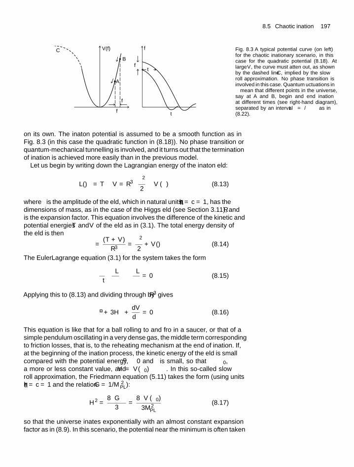
8.5 Chaotic inflation 197
Δf
ΔfΔt
f
fV(f)
B
C
A
t
Fig. 8.3 A typical potential curve (on left)for the chaotic inflationary scenario, in thiscase for the quadratic potential (8.18). Atlarge V , the curve must flatten out, as shownby the dashed line C, implied by the ‘slowroll’ approximation. No phase transition isinvolved in this case. Quantum fluctuations inφ mean that different points in the universe,say at A and B, begin and end inflationat different times (see right-hand diagram),separated by an interval �t = �φ/φ as in(8.22).
on its own. The inflaton potential is assumed to be a smooth function as inFig. 8.3 (in this case the quadratic function in (8.18)). No phase transition orquantum-mechanical tunnelling is involved, and it turns out that the terminationof inflation is achieved more easily than in the previous model.
Let us begin by writing down the Lagrangian energy of the inflaton field:
L(φ) = T − V = R3[φ2
2− V (φ)
](8.13)
where φ is the amplitude of the field, which in natural units, h = c = 1, has thedimensions of mass, as in the case of the Higgs field (see Section 3.11), and Ris the expansion factor. This equation involves the difference of the kinetic andpotential energies T and V of the field as in (3.1). The total energy density ofthe field is then
ρφ = (T + V )
R3= φ2
2+ V (φ) (8.14)
The Euler–Lagrange equation (3.1) for the system takes the form
∂
∂t
(∂L
∂φ
)− ∂L
∂φ= 0 (8.15)
Applying this to (8.13) and dividing through by R3 gives
φ + 3H φ + dV
dφ= 0 (8.16)
This equation is like that for a ball rolling to and fro in a saucer, or that of asimple pendulum oscillating in a very dense gas, the middle term correspondingto friction losses, that is, to the reheating mechanism at the end of inflation. If,at the beginning of the inflation process, the kinetic energy of the field is smallcompared with the potential energy, φ ≈ 0 and φ is small, so that φ ≈ φ0,a more or less constant value, and V = V (φ0) ≈ ρφ. In this so-called slowroll approximation, the Friedmann equation (5.11) takes the form (using unitsh = c = 1 and the relation G = 1/M 2
PL):
H 2 = 8πGρφ
3= 8πV (φ0)[
3M 2PL
] (8.17)
so that the universe inflates exponentially with an almost constant expansionfactor as in (8.9). In this scenario, the potential near the minimum is often taken
198 Development of structure in the early universe
to be of the simple quadratic form
V (φ) = 1
2m2φ2 (8.18)
As the inflation proceeds, φ starts by changing slowly as V ‘rolls’ gently downthe dashed part of the curve in Fig. 8.3. With φ ≈ 0, (8.16) and (8.18) give
φ = −m2φ
3H(8.19)
and integrating we obtain
φ = φ0 exp
(−m2�t
3H
)(8.20)
where �t = t2 − t1 is the period of inflation as in (8.11). Clearly, φ shouldnot fall too rapidly or the full expansion will not be obtained, and inserting thelimit from (8.11) we therefore find from (8.20) that
60 < H�t <3H 2
m2
and hence from (8.17) and (8.18) the condition
m
MPL<
(2π
15
)1/2
(8.21)
This condition, imposed to ensure that a large enough inflation factor is obtained,also shows that the energy density in the inflaton field is comfortably lessthan M 4
PL, at which level unknown quantum gravitational effects could becomeimportant. Eventually the system rolls into the potential well of the true vacuumand inflation ceases, and as explained above, the to-and-fro oscillations in thewell correspond to the reheating phase.
There are many other models of inflation, including those which incorporatesupergravity, but we do not discuss them here. None seems yet to have beentotally successful in providing exactly the conditions required, but there seemslittle doubt that an inflationary scenario of some sort is an essential first stage inthe early development of the universe. There are two strong predictions of suchmodels. The first is that the closure parameter �tot must be extremely close tounity, that is, the curvature parameter k must be near zero, and the universe onvery large scales must be flat. The second is that only one particular patch ofthe early universe, out of the many, would have been in the correct state at thechosen time when the quantum fluctuation described in the next section tookplace; there must have been many other universes growing from other suchpatches. So, enormous as is our universe, inflation suggests that it is but a dotin the ocean, a tiny part of a much larger space domain.
8.6 Quantum fluctuations and inflation
It is believed that quantum fluctuations are at the heart of anisotropies in theearly universe. In Chapter 3, we saw that quantum fluctuations in elementary
8.6 Quantum fluctuations and inflation 199
particle physics, in the form, for example, of the creation and annihilationof virtual electron–positron pairs, were able to account for the anomalousmagnetic moments of the electron and the muon, and that such fluctuationsare a vital part of the very successful electroweak theory. In a static universe,such virtual processes could not result in production of real particles, since paircreation will always be followed by annihilation. However, in the inflationaryscenario, the rapid expansion implies that any virtual particle–antiparticle pairswhich are created would not be able to annihilate completely. Both creationand annihilation rates are the product of particle densities and interaction cross-sections. So a lower particle density at annihilation than for the previous processof creation would lead to a net creation of real particles (from the energy in theinflaton field). This is the mechanism assumed for particle (and antiparticle)creation in the early universe. Such quantum fluctuations are also involved,for example, in connection with Hawking radiation from black holes (seeSection 10.12).
Quantum fluctuations of course arise in the first place as a result of theuncertainty relation. In a particular time interval �t the energy of a systemcannot be specified to an accuracy better than �E, where �t · �E ∼ h.Fluctuations in the inflaton field amplitude φ can be thought of as due to thedifferent times at which different ‘bubble’ universes complete inflation as inFig. 8.3, via the relation
�t = �φ
φ(8.22)
When discussing fluctuations in the microwave background radiation in Section8.13 below, the amplitude of the fluctuations at the horizon scale are important,and they are determined by the different amounts that the universes haveexpanded:
�ρ
ρ= δhor = H�t ∼ H 2
φ(8.23)
where the Hubble time is 1/H and we have used the relation �φ ∼ H from theuncertainty principle (again in units h/2π = c = 1). Using equation (8.17) forH 2 and (8.19) for φ, we thus obtain for the estimated density fluctuation
�ρ
ρ∼(
m
MPL
)(φ
MPL
)2
(8.24)
We repeat that experimentally this quantity is of order 10−5. Ideally of courseit would be nice to predict the magnitude of the fluctuations from the inflationmodel, but at the present time this does not seem possible, since the numberexpected depends on the precise form assumed for the inflaton potential V (φ).
Perhaps, in the course of future studies of polarization of the CMB induced bygravitational waves accompanying inflation, as described in Sections 8.15 and8.16, it may prove possible to perfect the inflation model. At present, however,no definite predictions seem to be possible regarding the level of quantumfluctuations. Even so, the idea that the material universe, extending now to theorder of 1026 m, had its origins in a quantum fluctuation, which started offspace/time as we know it as a microcosm of radius 10−27 m is quite grandioseand appealing.
200 Development of structure in the early universe
8.7 The spectrum of primordial fluctuations
The quantum fluctuations referred to above are ‘zero-point’ oscillations inthe cosmic fluid. As soon as inflation commences, however, at superluminalvelocity, most of the fluid will move outside the horizon scale 1/H . (We recallhere that the horizon distance is of order ct where t is the time after the beginningof the expansion, and in units c = 1 is equal to the reciprocal of the expansionrate 1/H ). This means that there will no longer be communication between thecrests and the troughs of the oscillations: the quantum fluctuations are therefore‘frozen’ as classical density fluctuations at the super-horizon scale. We alsonote from (8.24) that since no particular distance scale is specified for thefluctuations, the spectrum of fluctuations should follow a power law, which(unlike an exponential, for example) does not involve any absolute scale. Thesefluctuations in density correspond to perturbations in the metric of space-timeassociated with variations in the curvature parameter. As discussed below, thereare different possible types of fluctuation; however, it is usually assumed thatthe perturbations are adiabatic, that is, that the density variations are the samein different components (baryons, photons, etc.).
We can see how the fluctuations depend on the index of the power lawdetermining the balance between small and large scales, using an argument dueto Barrow (1988). This is based on the idea that an exponential expansion isinvariant under a time translation. No matter at what time one fixes the start ofthe exponential growth, the universe will look the same at every epoch. Thusthe expansion rate H is constant, the density ρ is constant, the horizon distance1/H is constant, and the universe is effectively in a stationary state. No timeor place can then have significance over any other, with the result that theamplitude of the perturbations in the metric structure must be the same on alllength scales as they enter the horizon—otherwise a change in the magnitude ofthe perturbation could be used to indicate a time sense. This metric (curvatureof space) is determined by the gravitational potential �, and in the absenceof time dependence, this will obey Poisson’s Equation of Newtonian gravity(see (2.20)):
∇2� = 4πGρ (8.25)
Assuming spherical symmetry, ∇2� = (1/r2) [
∂(r2∂�
/∂r)∂r], and the
solution is
�(r) = 2πGρr2
3(8.26)
On the scale of the horizon distance rHor = 1/H , which is the only naturallength in the problem, we have therefore
� = 2πGρ
3H 2
while on some arbitrary scale λ < 1/H , fluctuations in the gravitationalpotential due to fluctuations �ρ in density will be
�� = 2πG�ρλ2
3(8.27)
8.7 The spectrum of primordial fluctuations 201
Hence the fractional perturbation in the gravitational potential on the scale λ
has the value
��
�= H 2λ2 �ρ
ρ(8.28)
As explained above, in a stationary state, ��/� must be some constantindependent of the arbitrary distance scale λ. Since H is also approximatelyconstant, it follows that the density fluctuation, as it comes inside the horizon(and specifically its root mean square value) must have a spectrum with thepower law dependence on λ of
⟨δ2λ
⟩1/2 =(
�ρ
ρ
)rms
∼ 1
λ2(8.29)
known as the PHZ (Peebles–Harrison–Zeldovich) spectrum, typical of theinflationary scenario. In words, this spectrum gives the universe the same degreeof ‘wrinkliness’ and the same amplitude for the perturbations on the horizon,independent of the epoch, as would be expected for a stationary state. For thisreason the above spectrum is called scale-invariant.
Notice that the fluctuations predicted are actually smaller than the purelystatistical fluctuations on the number N of particles contained in the volume λ3,since according to (8.29), �N/N ∝ N−2/3, while for a statistical fluctuation�N/N ∝ N−1/2. This smoothing out of fluctuations on large scales is anexample of a general rule that, as we shall see below, in an accelerating universe,perturbations tend to decay, while in a decelerating universe, perturbations tendto grow with time.
Rather than describing the dependence of the fluctuations on the length scaleλ, it is usual to discuss their Fourier decomposition in terms of the wavenumberk = 2π/λ. First we define the density contrast at space coordinate x, asthe fractional deviation from the value 〈ρ〉 of the density averaged over thenormalization volume:
δ(x) = [ρ(x) − 〈ρ〉]〈ρ〉
The two-point correlation function for points in space separated by distance ris given by
ξ(r) = 〈δ(x + r)δ(x)〉
again averaged over all pairs of points in the volume. This correlation functionis then expressed as a Fourier integral over the wave number k. Assumingthat the phases of the fluctuations are random, cross terms will cancel and oneobtains:
ξ(r) =∫
|δ(k)|2 exp (ik · r) d3k (8.30)
Here, for simplicity, some factors of 2π in the definition of the Fourier transformhave been omitted. The quantity P(k) = |δ(k)|2 is referred to as the power ofthe fluctuation spectrum. Assuming isotropy, one can integrate over polar and
202 Development of structure in the early universe
azimuthal angles:
ξ(r) =∫∫
|δ (k)|2 exp (ikr cos θ) 2π d(cos θ)k2 dk
Taking the limits +1 and -1 for cos θ, the angular integration gives
ξ(r) = 4π
∫P (k)
[(sin kr)
kr
]k2 dk (8.31)
From this expression, we see that for values of kr � 1, the term in squarebrackets, and hence the integrand, will average to zero, while for values ofkr < 1, the integral will vary as k3P(k). Because of the absence of any absolutescale, P(k) ∼ kn must be represented by a power law, and for the inflationarymodel, we already know from the above analysis that n = 1. Thus ξ ∼ k4,and the square root of the correlation function then varies as k2 or 1/λ2, aswe already deduced in (8.29). As described below, analysis of the angularfluctuations of the CMB leads to an experimental determination of the index nfrom the WMAP experiment (see data summary by Yao et al. 2006):
n = 0.95 ± 0.02 (8.32)
anddn
d(ln k)= −0.003 ± 0.010
This result is close to n = 1 as predicted by inflation. However, there are smalldeviations or ‘tilt’ (1 − n) from this unit value, which are significant here at the2σ level. These arise if one takes into account that during inflation ϕ and ϕ areslightly different from zero. The result in the second line above indicates nosignificant ‘running’ of the index with the wave number.
8.8 Large-scale structures: gravitationalcollapse and the Jeans mass
In Chapter 5 the early universe was described as a homogeneous, isotropic andperfect primordial fluid (a perfect fluid being one in which frictional effectsare negligible), undergoing a universal expansion. In contrast, the universetoday is ‘grainy’ with the matter clumped into billions of individual galaxies,each containing of order 1011 stars, and separated from their neighbours byenormous voids in space. Starting off from the Big Bang, we have to ask whatwere the physical processes taking place which led to such structures. Thedevelopments on the smallest scales, that of the stars themselves, are dealtwith in Chapter 10. Here we discuss the large-scale structures which were,we believe, originally seeded by tiny fluctuations in the inflationary phasedescribed above, which are detectable today in observations on the microwavebackground radiation, as described in Sections 8.13–8.15. However, beforediscussing those observations and their interpretation, we consider the generalconditions necessary for gravitational collapse of a classical gas cloud, asoriginally enunciated by Jeans.
8.8 Gravitational collapse and the Jeans mass 203
Let us first estimate the time required for a cloud of ordinary gas to collapseunder gravity, assuming to begin with that gas pressure can be neglected.Suppose that the cloud is spherical, of constant mass M and of initial radius r0,and that it begins gravitational contraction. When the radius has shrunk to r, asmall mass m in the outermost shell will have lost gravitational potential energyGMm (1/r − 1/r0) and gained kinetic energy (m/2) (dr/dt)2, assuming that itwas initially at rest. Equating these two, we get for the time of free fall fromr = r0 to r = 0
tFF =∫
dr(dr/
dt) =∫ (
2GM
r− 2GM
r0
)−1/2
dr (8.33)
Substituting r = r0 sin2θ and with the limits θ = π/2 and 0, this integral gives
tFF =(π
2
)( r30
2GM
)1/2
=(
3π
32Gρ
)1/2
(8.34)
where ρ is the mean initial density of the cloud. Note that the result isindependent of the radius, for a given initial density. This free fall time, itmay be observed, is comparable with the circulation time of a satellite in closeorbit about the initial cloud, equal to (3π/Gρ)1/2.
As the cloud of gas condenses, gravitational potential energy will betransformed into kinetic (heat) energy of the gas particles. If these are atomsor molecules, this motional kinetic energy may be absorbed through collisionaldissociation of molecules or ionization of atoms, as well as resulting in atomicexcitation which can be radiated away as photons if the cloud is transparent.These processes absorb and then re-emit the gravitational energy liberated andallow the cloud to contract further, but eventually hydrostatic equilibrium willbe attained when the pressure of the heated gas balances the inward gravitationalpressure. The total kinetic energy of the gas at temperature T will be
Ekin =(
3
2
)MkT
m(8.35)
where m is the mass per particle, M /m is the total number of particles, and 3kT/2is the mean energy per particle at temperature T . The gravitational potentialenergy of a sphere of mass M and radius r is
Egrav ≈ GM 2
r(8.36)
where there is a numerical coefficient of order unity, depending on the variationof density with radius (and equal to 3/5 if the density is constant). Comparingthese two expressions, we find that a cloud will condense if Egrav � Ekin, thatis, if r and ρ exceed the critical values
rcrit = 2M Gm
(3kT )=(
3
2
)(kT
2πρGm
)1/2
(8.37)
ρcrit =(
3
4πM 2
)(3kT
2mG
)3
204 Development of structure in the early universe
Example 8.2 Calculate the critical density and radius of a cloud ofmolecular hydrogen with a mass of 10,000 solar masses at a temperatureof 20K.
Inserting the values in SI units of Msun = 2 × 1030, G = 6.67 × 10⁻¹¹,k = 1.38 × 10⁻²³ and m = 3 × 10⁻²⁷ kg into equations (8.37) gives thevalues
rcrit = 1.07 × 10¹⁹ m = 0.35 kpc
ρcrit = 3.83 × 10⁻²⁴ kg m−3 = 1150 mols m−3
These are typical temperature and density values for clouds of gas inglobular clusters, which each contain of order 105 stars. Individual starswill form as a result of density fluctuations in the cloud, requiring from(8.37) gas densities about 108 times larger.
From the viewpoint of the development of large-scale structure in theuniverse, we want to determine which criteria lead to a cloud of gas condensingas a result of an upward fluctuation in density in one part of it. In terms of thedensity ρ, there is a critical size of the cloud called the Jeans length with a value
λJ = vs
(π
Gρ
)1/2
(8.38)
obtained essentially by multiplying the sound velocity by the free-fall time. Themass of a cloud of diameter equal to the Jeans length is called the Jeans mass
MJ = πρλ3J
6(8.39)
Here vs is the velocity of sound in the gas. What do these equations mean?The typical time for sound waves (propagated as a result of any densityperturbations) to cross a cloud of size L is L/vs, and this is less than thegravitational collapse time (8.34) when L λJ. So the perturbation just resultsin sound waves oscillating to and fro, and there is no preferred location towardswhich matter can gravitate. On the other hand, if L � λJ, sound waves cannottravel fast enough to respond to density perturbations and the cloud will start tocondense around them. For a cloud of non-relativistic matter, the Jeans lengthλJ in (8.38) and rcrit in (8.37) are of course one and the same (up to numericalfactors of order unity). For then
v2s = ∂P
∂ρ= γkT
m(8.40)
where γ is the ratio of specific heats, equal to 5/3 in neutral hydrogen. In thatcase
λJ =(
5πkT
3Gρm
)1/2
(8.41)
Thus in terms of the temperature of non-relativistic gas particles, both rcrit in(8.37) and λJ in (8.38) are of the order of magnitude (kT/Gρm)1/2.
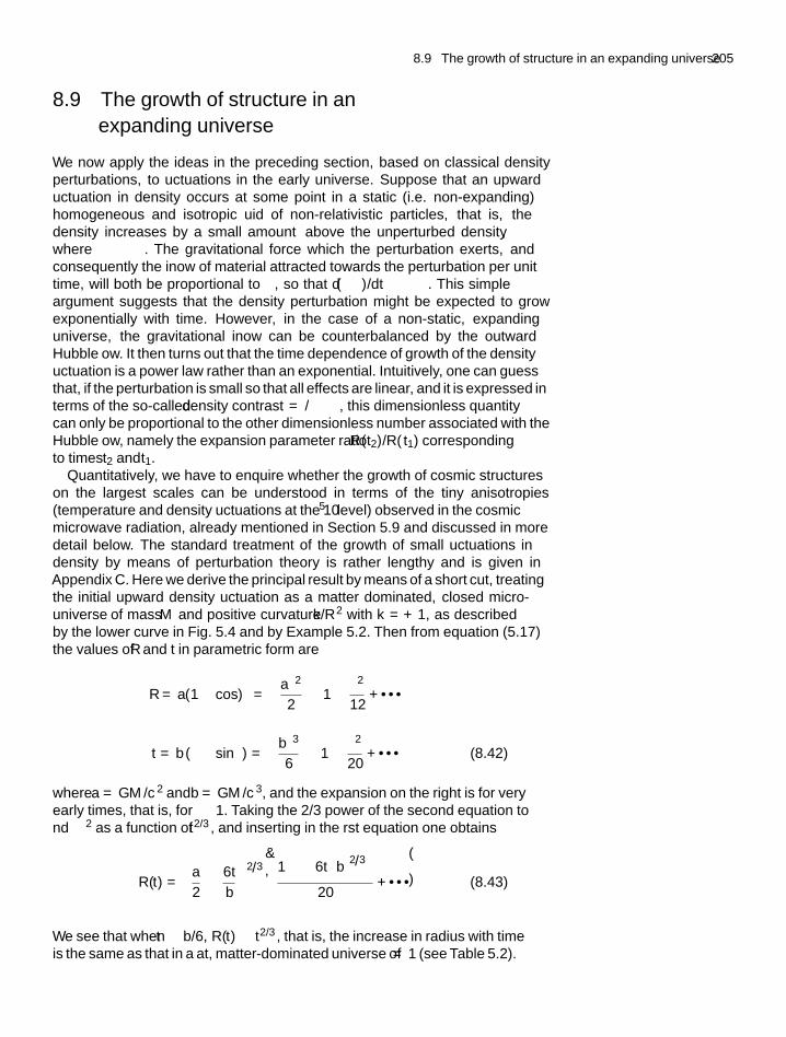
8.9 The growth of structure in an expanding universe 205
8.9 The growth of structure in anexpanding universe
We now apply the ideas in the preceding section, based on classical densityperturbations, to fluctuations in the early universe. Suppose that an upwardfluctuation in density occurs at some point in a static (i.e. non-expanding)homogeneous and isotropic fluid of non-relativistic particles, that is, thedensity increases by a small amount �ρ above the unperturbed density ρ,where �ρ ρ. The gravitational force which the perturbation exerts, andconsequently the inflow of material attracted towards the perturbation per unittime, will both be proportional to �ρ, so that d (�ρ)/dt ∝ �ρ. This simpleargument suggests that the density perturbation might be expected to growexponentially with time. However, in the case of a non-static, expandinguniverse, the gravitational inflow can be counterbalanced by the outwardHubble flow. It then turns out that the time dependence of growth of the densityfluctuation is a power law rather than an exponential. Intuitively, one can guessthat, if the perturbation is small so that all effects are linear, and it is expressed interms of the so-called density contrast δ = �ρ/ρ, this dimensionless quantitycan only be proportional to the other dimensionless number associated with theHubble flow, namely the expansion parameter ratio R (t2)/R(t1) correspondingto times t2 and t1.
Quantitatively, we have to enquire whether the growth of cosmic structureson the largest scales can be understood in terms of the tiny anisotropies(temperature and density fluctuations at the 10−5 level) observed in the cosmicmicrowave radiation, already mentioned in Section 5.9 and discussed in moredetail below. The standard treatment of the growth of small fluctuations indensity by means of perturbation theory is rather lengthy and is given inAppendix C. Here we derive the principal result by means of a short cut, treatingthe initial upward density fluctuation as a matter dominated, closed ‘micro-universe’ of mass M and positive curvature k/R2 with k = +1, as describedby the lower curve in Fig. 5.4 and by Example 5.2. Then from equation (5.17)the values of R and t in parametric form are
R = a(1 − cos θ) =(
aθ2
2
)[1 − θ2
12+ · · ·
]
t = b (θ − sin θ) =(
bθ3
6
)[1 − θ2
20+ · · ·
](8.42)
where a = GM /c2 and b = GM /c3, and the expansion on the right is for veryearly times, that is, for θ 1. Taking the 2/3 power of the second equation tofind θ2 as a function of t2/3, and inserting in the first equation one obtains
R(t) =(a
2
)(6t
b
)2/3⎡⎣1 −
[(6t/
b)2/3]
20+ · · ·
⎤⎦ (8.43)
We see that when t b/6, R(t) ∝ t2/3, that is, the increase in radius with timeis the same as that in a flat, matter-dominated universe of � = 1 (see Table 5.2).
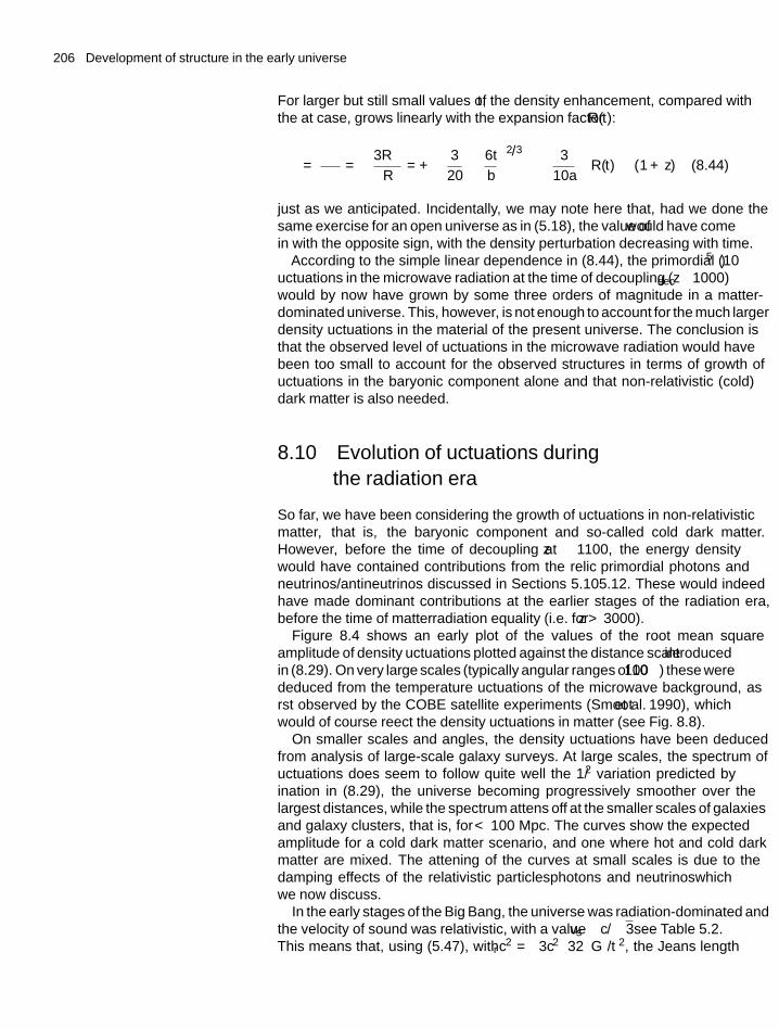
206 Development of structure in the early universe
For larger but still small values of t, the density enhancement, compared withthe flat case, grows linearly with the expansion factor R(t):
δ = �ρ
ρ= −3�R
R= +
(3
20
)[6t
b
]2/3
≈(
3
10a
)R(t) ∝ (1 + z) (8.44)
just as we anticipated. Incidentally, we may note here that, had we done thesame exercise for an open universe as in (5.18), the value of δ would have comein with the opposite sign, with the density perturbation decreasing with time.
According to the simple linear dependence in (8.44), the primordial (10−5)
fluctuations in the microwave radiation at the time of decoupling (zdec ∼ 1000)would by now have grown by some three orders of magnitude in a matter-dominated universe. This, however, is not enough to account for the much largerdensity fluctuations in the material of the present universe. The conclusion isthat the observed level of fluctuations in the microwave radiation would havebeen too small to account for the observed structures in terms of growth offluctuations in the baryonic component alone and that non-relativistic (cold)dark matter is also needed.
8.10 Evolution of fluctuations duringthe radiation era
So far, we have been considering the growth of fluctuations in non-relativisticmatter, that is, the baryonic component and so-called cold dark matter.However, before the time of decoupling at z ∼ 1100, the energy densitywould have contained contributions from the ‘relic’ primordial photons andneutrinos/antineutrinos discussed in Sections 5.10–5.12. These would indeedhave made dominant contributions at the earlier stages of the radiation era,before the time of matter–radiation equality (i.e. for z > 3000).
Figure 8.4 shows an early plot of the values of the root mean squareamplitude of density fluctuations plotted against the distance scale λ introducedin (8.29). On very large scales (typically angular ranges of 10◦–100◦) these werededuced from the temperature fluctuations of the microwave background, asfirst observed by the COBE satellite experiments (Smoot et al. 1990), whichwould of course reflect the density fluctuations in matter (see Fig. 8.8).
On smaller scales and angles, the density fluctuations have been deducedfrom analysis of large-scale galaxy surveys. At large scales, the spectrum offluctuations does seem to follow quite well the 1/λ2 variation predicted byinflation in (8.29), the universe becoming progressively smoother over thelargest distances, while the spectrum flattens off at the smaller scales of galaxiesand galaxy clusters, that is, for λ < 100 Mpc. The curves show the expectedamplitude for a cold dark matter scenario, and one where hot and cold darkmatter are mixed. The flattening of the curves at small scales is due to thedamping effects of the relativistic particles—photons and neutrinos—whichwe now discuss.
In the early stages of the Big Bang, the universe was radiation-dominated andthe velocity of sound was relativistic, with a value vs ∼ c/
√3—see Table 5.2.
This means that, using (5.47), with ρrc2 = (3c2/
32πG)/t2, the Jeans length
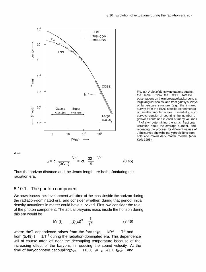
8.10 Evolution of fluctuations during the radiation era 207
Galaxyclusters
Superclusters
1
10–1
10
10–2
102
10–3
10– 4
l(Mpc)
COBE
CDM
70% CDM 30% HDM
1/λ2
(Δ�/
�) r
ms
Lum
pySm
ooth
LSS
Largescales
10 102 1031
Fig. 8.4 Aplot of density fluctuations againstthe scale λ, from the COBE satelliteobservations on the microwave background atlarge angular scales, and from galaxy surveysof large-scale structure (e.g. the infraredsurvey from the IRAS satellite experiments)on smaller angular scales. Essentially, suchsurveys consist of counting the number ofgalaxies contained in each of many volumesλ3 of sky, determining the r.m.s. fractionalfluctuation about the average number, andrepeating the process for different values ofλ. The curves show the early predictions fromcold and mixed dark matter models (afterKolb 1998).
was
λJ = c
[π
(3Gρr)
]1/2
= ct
(32π
9
)1/2
(8.45)
Thus the horizon distance and the Jeans length are both of order ct during theradiation era.
8.10.1 The photon component
We now discuss the development with time of the mass inside the horizon duringthe radiation-dominated era, and consider whether, during that period, initialdensity fluctuations in matter could have survived. First, we consider the roleof the photon component. The actual baryonic mass inside the horizon duringthis era would be
MH(t) ∼ ρb(t)(ct)3 ∝ 1
T 3(8.46)
where the T dependence arises from the fact that ρb ∝ 1/R3 ∝ T 3 andfrom (5.49), t ∝ 1/T 2 during the radiation-dominated era. This dependencewill of course flatten off near the decoupling temperature because of theincreasing effect of the baryons in reducing the sound velocity. At thetime of baryon–photon decoupling, zdec ∼ 1100, ρb=ρc�b(1 + zdec)
3, and
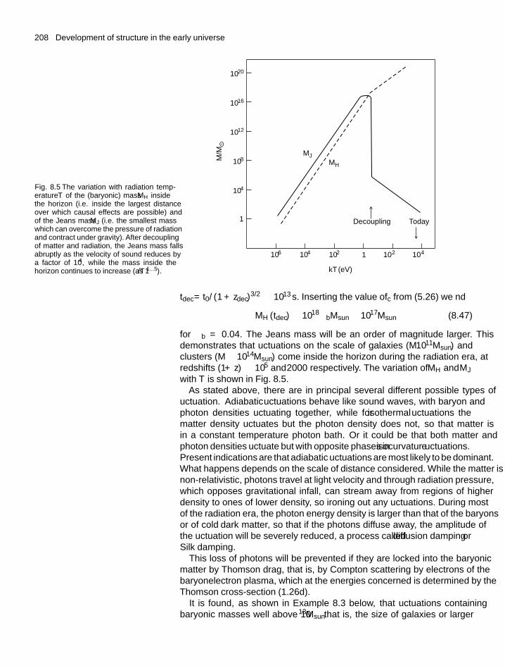
208 Development of structure in the early universe
Fig. 8.5 The variation with radiation temp-erature T of the (baryonic) mass MH insidethe horizon (i.e. inside the largest distanceover which causal effects are possible) andof the Jeans mass MJ (i.e. the smallest masswhich can overcome the pressure of radiationand contract under gravity). After decouplingof matter and radiation, the Jeans mass fallsabruptly as the velocity of sound reduces bya factor of 104, while the mass inside thehorizon continues to increase (as 1/T 1...5).
Decoupling Today
kT (eV)
MJMH
M/M
1020
1016
1
104
108
1012
106 104 102 1 10 –2 10 –4
tdec = t0/(1 + zdec)3/2 ∼ 1013 s. Inserting the value of ρc from (5.26) we find
MH (tdec) ∼ 1018�bMsun ∼ 1017Msun (8.47)
for �b = 0.04. The Jeans mass will be an order of magnitude larger. Thisdemonstrates that fluctuations on the scale of galaxies (M ∼ 1011Msun) andclusters (M ∼ 1014Msun) come inside the horizon during the radiation era, atredshifts (1 + z) ∼ 105 and ∼2000 respectively. The variation of MH and MJ
with T is shown in Fig. 8.5.As stated above, there are in principal several different possible types of
fluctuation. Adiabatic fluctuations behave like sound waves, with baryon andphoton densities fluctuating together, while for isothermal fluctuations thematter density fluctuates but the photon density does not, so that matter isin a constant temperature photon bath. Or it could be that both matter andphoton densities fluctuate but with opposite phases in isocurvature fluctuations.Present indications are that adiabatic fluctuations are most likely to be dominant.What happens depends on the scale of distance considered. While the matter isnon-relativistic, photons travel at light velocity and through radiation pressure,which opposes gravitational infall, can stream away from regions of higherdensity to ones of lower density, so ironing out any fluctuations. During mostof the radiation era, the photon energy density is larger than that of the baryonsor of ‘cold’ dark matter, so that if the photons diffuse away, the amplitude ofthe fluctuation will be severely reduced, a process called diffusion damping orSilk damping.
This loss of photons will be prevented if they are locked into the baryonicmatter by ‘Thomson drag’, that is, by Compton scattering by electrons of thebaryon–electron plasma, which at the energies concerned is determined by theThomson cross-section (1.26d).
It is found, as shown in Example 8.3 below, that fluctuations containingbaryonic masses well above 1013Msun—that is, the size of galaxies or larger
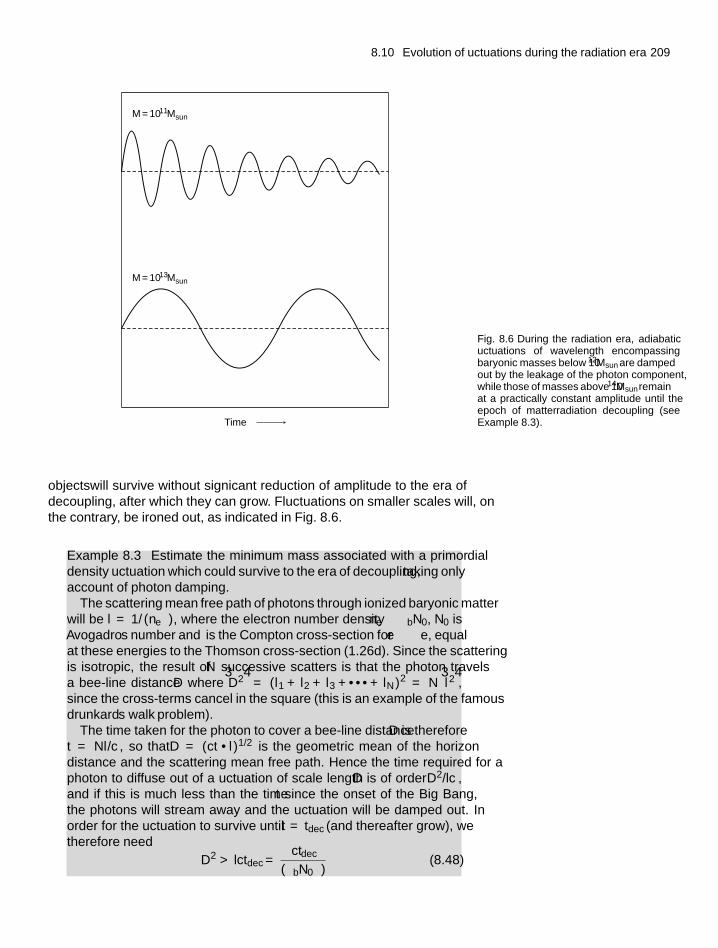
8.10 Evolution of fluctuations during the radiation era 209
M = 1011Msun
M = 1013Msun
Time
Fig. 8.6 During the radiation era, adiabaticfluctuations of wavelength encompassingbaryonic masses below 1012Msun are dampedout by the leakage of the photon component,while those of masses above 1014Msun remainat a practically constant amplitude until theepoch of matter–radiation decoupling (seeExample 8.3).
objects—will survive without significant reduction of amplitude to the era ofdecoupling, after which they can grow. Fluctuations on smaller scales will, onthe contrary, be ironed out, as indicated in Fig. 8.6.
Example 8.3 Estimate the minimum mass associated with a primordialdensity fluctuation which could survive to the era of decoupling, taking onlyaccount of photon damping.
The scattering mean free path of photons through ionized baryonic matterwill be l = 1/(neσ), where the electron number density ne ∼ ρbN0, N0 isAvogadro’s number and σ is the Compton cross-section for γe → γe, equalat these energies to the Thomson cross-section (1.26d). Since the scatteringis isotropic, the result of N successive scatters is that the photon travelsa bee-line distance D where
⟨D2⟩ = (l1 + l2 + l3 + · · · + lN )2 = N
⟨l2⟩,
since the cross-terms cancel in the square (this is an example of the famous‘drunkard’s walk’ problem).
The time taken for the photon to cover a bee-line distance D is thereforet = Nl/c, so that D = (ct · l)1/2 is the geometric mean of the horizondistance and the scattering mean free path. Hence the time required for aphoton to diffuse out of a fluctuation of scale length D is of order D2/lc,and if this is much less than the time t since the onset of the Big Bang,the photons will stream away and the fluctuation will be damped out. Inorder for the fluctuation to survive until t = tdec (and thereafter grow), wetherefore need
D2 > lctdec = ctdec
(ρbN0σ)(8.48)
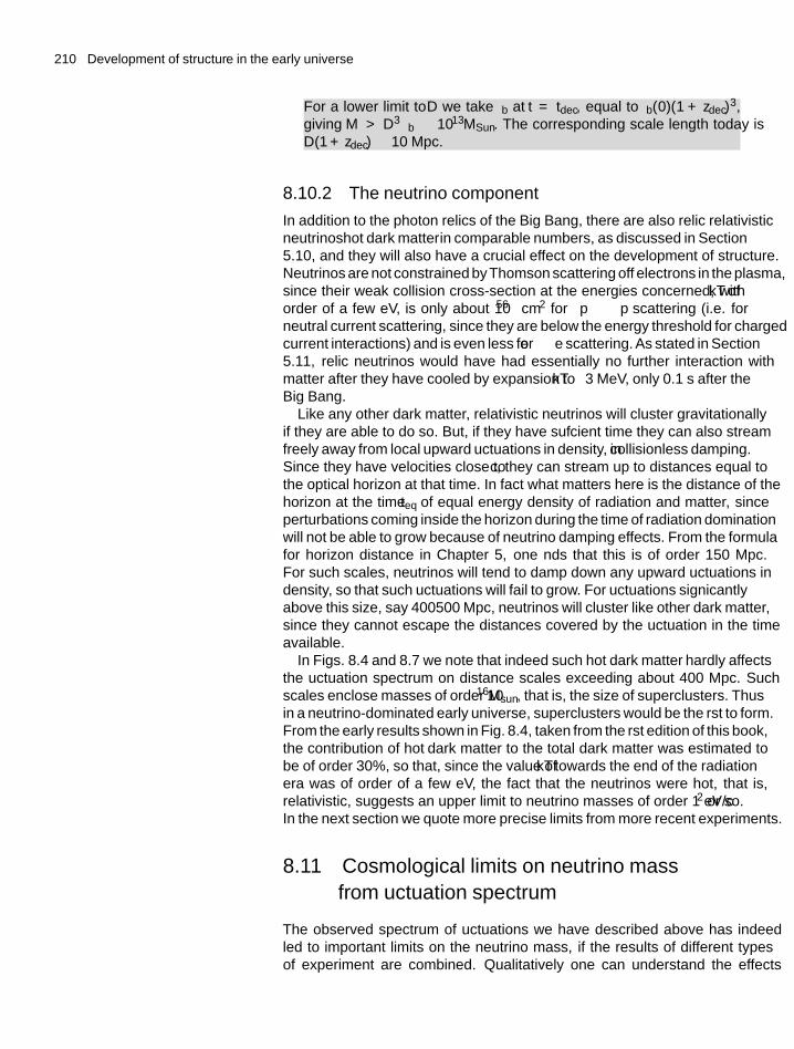
210 Development of structure in the early universe
For a lower limit to D we take ρb at t = tdec, equal to ρb(0)(1 + zdec)3,
giving M > D3ρb ∼ 1013MSun. The corresponding scale length today isD(1 + zdec) ∼ 10 Mpc.
8.10.2 The neutrino component
In addition to the photon relics of the Big Bang, there are also relic relativisticneutrinos—‘hot dark matter’—in comparable numbers, as discussed in Section5.10, and they will also have a crucial effect on the development of structure.Neutrinos are not constrained by Thomson scattering off electrons in the plasma,since their weak collision cross-section at the energies concerned, with kT oforder of a few eV, is only about 10−56 cm2 for νp → νp scattering (i.e. forneutral current scattering, since they are below the energy threshold for chargedcurrent interactions) and is even less for νe → νe scattering. As stated in Section5.11, relic neutrinos would have had essentially no further interaction withmatter after they have cooled by expansion to kT ∼ 3 MeV, only 0.1 s after theBig Bang.
Like any other dark matter, relativistic neutrinos will cluster gravitationallyif they are able to do so. But, if they have sufficient time they can also streamfreely away from local upward fluctuations in density, in collisionless damping.Since they have velocities close to c, they can stream up to distances equal tothe optical horizon at that time. In fact what matters here is the distance of thehorizon at the time teq of equal energy density of radiation and matter, sinceperturbations coming inside the horizon during the time of radiation dominationwill not be able to grow because of neutrino damping effects. From the formulafor horizon distance in Chapter 5, one finds that this is of order 150 Mpc.For such scales, neutrinos will tend to damp down any upward fluctuations indensity, so that such fluctuations will fail to grow. For fluctuations significantlyabove this size, say 400–500 Mpc, neutrinos will cluster like other dark matter,since they cannot escape the distances covered by the fluctuation in the timeavailable.
In Figs. 8.4 and 8.7 we note that indeed such ‘hot dark matter’ hardly affectsthe fluctuation spectrum on distance scales exceeding about 400 Mpc. Suchscales enclose masses of order 1016Msun, that is, the size of superclusters. Thusin a neutrino-dominated early universe, superclusters would be the first to form.From the early results shown in Fig. 8.4, taken from the first edition of this book,the contribution of ‘hot’ dark matter to the total dark matter was estimated tobe of order 30%, so that, since the value of kT towards the end of the radiationera was of order of a few eV, the fact that the neutrinos were ‘hot’, that is,relativistic, suggests an upper limit to neutrino masses of order 1 eV/c2 or so.In the next section we quote more precise limits from more recent experiments.
8.11 Cosmological limits on neutrino massfrom fluctuation spectrum
The observed spectrum of fluctuations we have described above has indeedled to important limits on the neutrino mass, if the results of different typesof experiment are combined. Qualitatively one can understand the effects
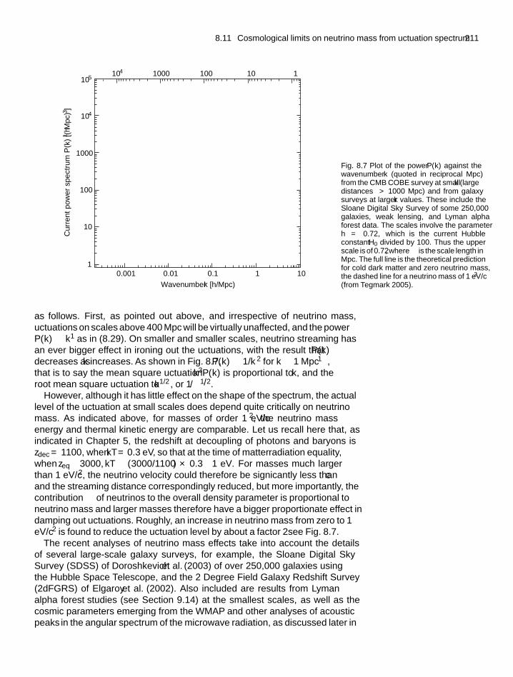
8.11 Cosmological limits on neutrino mass from fluctuation spectrum 211
105104 1000 100 10 1
104
100
1000
Cur
rent
pow
er s
pect
rum
P(k
) [(
h–1 M
pc)3 ]
10
10.001 0.01
Wavenumber k [h/Mpc)
0.1 1 10
Fig. 8.7 Plot of the power P(k) against thewavenumber k (quoted in reciprocal Mpc)from the CMB COBE survey at small k (largedistances λ > 1000 Mpc) and from galaxysurveys at larger k values. These include theSloane Digital Sky Survey of some 250,000galaxies, weak lensing, and Lyman alphaforest data. The scales involve the parameterh = 0.72, which is the current Hubbleconstant H0 divided by 100. Thus the upperscale is of 0.72 λ, where λ is the scale length inMpc. The full line is the theoretical predictionfor cold dark matter and zero neutrino mass,the dashed line for a neutrino mass of 1 eV/c2
(from Tegmark 2005).
as follows. First, as pointed out above, and irrespective of neutrino mass,fluctuations on scales above 400 Mpc will be virtually unaffected, and the powerP(k) ∼ k1 as in (8.29). On smaller and smaller scales, neutrino streaming hasan ever bigger effect in ironing out the fluctuations, with the result that P(k)
decreases as k increases. As shown in Fig. 8.7, P(k) ∼ 1/k2 for k ∼ 1 Mpc−1,that is to say the mean square fluctuation k3P(k) is proportional to k, and theroot mean square fluctuation to k1/2, or 1/λ1/2.
However, although it has little effect on the shape of the spectrum, the actuallevel of the fluctuation at small scales does depend quite critically on neutrinomass. As indicated above, for masses of order 1 eV/c2, the neutrino massenergy and thermal kinetic energy are comparable. Let us recall here that, asindicated in Chapter 5, the redshift at decoupling of photons and baryons iszdec = 1100, when kT = 0.3 eV, so that at the time of matter–radiation equality,when zeq ∼ 3000, kT ∼ (3000/1100) × 0.3 ∼ 1 eV. For masses much largerthan 1 eV/c2, the neutrino velocity could therefore be significantly less than cand the streaming distance correspondingly reduced, but more importantly, thecontribution �ν of neutrinos to the overall density parameter is proportional toneutrino mass and larger masses therefore have a bigger proportionate effect indamping out fluctuations. Roughly, an increase in neutrino mass from zero to 1eV/c2 is found to reduce the fluctuation level by about a factor 2—see Fig. 8.7.
The recent analyses of neutrino mass effects take into account the detailsof several large-scale galaxy surveys, for example, the Sloane Digital SkySurvey (SDSS) of Doroshkevich et al. (2003) of over 250,000 galaxies usingthe Hubble Space Telescope, and the 2 Degree Field Galaxy Redshift Survey(2dFGRS) of Elgaroy et al. (2002). Also included are results from ‘Lymanalpha forest’ studies (see Section 9.14) at the smallest scales, as well as thecosmic parameters emerging from the WMAP and other analyses of ‘acousticpeaks’ in the angular spectrum of the microwave radiation, as discussed later in
212 Development of structure in the early universe
this chapter. The important point about this combined information of differentcosmological parameters, is that it provides the normalization between smallscale fluctuations from galaxy surveys, and the large-scale fluctuations fromthe COBE experiments on the microwave background, thus placing strongerconstraints on the neutrino contribution. Recent analyses (Tegmark 2005) areconsistent with zero neutrino mass and lead to an upper bound for the masssummed over all flavours (90% confidence level):∑
mv(e, μ, τ) < 0.42eV
c2(8.49)
This limit is already almost within an order of magnitude of the minimum massvalues from neutrino oscillations (see Chapter 4), and will surely improve inthe near future.
Incidentally, at this point it may be remarked that today, relic neutrinos haveno chance of clustering around galaxies or clusters. They are non-relativistic,with a value of kT = 0.17 meV (see Section 5.10) compared with massdifferences from (4.12)—and by inference the masses themselves—of up toat least 10–50 meV. The mean velocity of their Maxwell energy distributionwould be ∼6000 km s−1 for a neutrino mass of 1 eV/c2, and ∼20,000 km s−1
for a mass of 0.1 eV/c2. Either of these velocities is way beyond the escapevelocity from galaxies or clusters (see Problem 8.8).
8.12 Growth of fluctuations in thematter-dominated era
As indicated in Example 8.4 below, as soon as matter and radiation decoupledand neutral atoms formed, the velocity of sound, and hence the Jeans length,decreased by over 10,000 times. Growth of inhomogeneities on galactic andsmaller scales then became possible.
Example 8.4 Estimate the value of the Jeans mass just after the epoch ofdecoupling of matter (baryons) and radiation.
After decoupling of baryonic matter from radiation and the recombinationof protons and electrons to form atoms, the velocity of sound is given by(8.40):
v2s
c2= 5kT
3mHc2
Taking kT = 0.3 eV from Section 5.12 and the mass energy of the hydrogenatom mHc2 = 0.94 GeV, we find
vs
c= 2 × 10⁻⁵
Thus, compared with the pre-decoupling epoch, the sound velocity andthe Jeans length have fallen by a factor of 104, and the Jeans mass from1018Msun to 106Msun. This last is the typical mass of globular clusters oforder 105 stars, which are some of the oldest objects in the sky (see Chapter10). Obviously, even larger objects such as galaxies and galaxy clusterswould have had no problem in condensing under gravity at this epoch.
8.13 Temperature fluctuations and anisotropies in the CMB 213
We can see from the above discussion that only after the universe becamematter dominated did perturbations really have a chance to grow. In thisrespect, dark matter, and specifically cold dark matter, plays a vital role inthe development of structures at the galactic and super-galactic level. It turnsout in fact that the calculated increase in density contrast with time, as describedabove and starting out from values of �ρ/ρ ∼ 10−5 following inflation, is notenough to account for the observed growth of galaxies and clusters, relyingsimply on the gravitational collapse of the baryonic component alone (with�b(0) ∼ 0.04), once it has decoupled from radiation at a redshift z ∼ 1100. Aspreviously stated, one requires substantial amounts of cold (i.e. non-relativistic)dark matter (with �dm(0) ∼ 0.20) as a component of the primordial universe.Unlike normal (baryonic) matter, this will not interact with radiation viaThomson scattering and it also begins to dominate over radiation at an earlierepoch (z ∼ 3000–5000, see Section 5.13), and thus is both more efficient atachieving gravitational collapse and has more time to achieve it. Of course,once the dark matter agglomerations have formed gravitational potential wells,baryons will fall into them and indeed their increase in density contrast willfollow that of the dark matter.
Finally, we note that the fluctuation spectrum, for example, that in Fig. 8.4,does seem to follow very well the 1/λ2 variation predicted on very largescales by the inflation scenario in (8.29), the universe becoming progressivelysmoother over the largest distances, while the spectrum flattens off at the smallerscales of galaxy clusters. This dependence on λ corresponds to the power lawP(k) ∼ kn in k-space, with n ≈ 1 as in (8.32), providing strong verification ofthe inflation scenario.
8.13 Temperature fluctuations andanisotropies in the CMB
So far we have been discussing the dependence of the density fluctuations ofmatter on scale length λ or wave number k. However, much of our presentknowledge of the basic parameters of the universe comes from the detailedand increasingly precise studies over the last 10 or 15 years of tiny (10−5)
temperature variations in the CMB in different directions in space, that is, theirangular dependence. Of course, via their interactions with the baryons, thephotons will suffer density and therefore temperature fluctuations which willmirror the fluctuations in matter density. We first briefly discuss the sources ofthese anisotropies, followed by a description of the experimental situation andits analysis.
The largest (10−3) effect observed is from the dipole term, mentioned inChapter 5, with the Doppler shift in temperature T (θ) = T0 [1 + (v/c) cos θ],arising from the ‘peculiar velocity’vector v (= 370 km s−1) of the Earth relativeto the Hubble flow. The COBE satellite observations also detected highermultipoles, which corresponded to variations in the temperature over angularscales of 7◦ or more, the scale being set by the detector resolution. Figure 8.8shows all-sky maps of the observed temperature fluctuations in the CMB, fromthe COBE and the more recent WMAP satellite experiments, the latter withangular resolution of order of a few minutes of arc. The temperature fluctuations
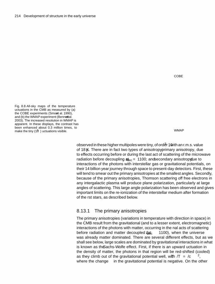
214 Development of structure in the early universe
Fig. 8.8 All-sky maps of the temperaturefluctuations in the CMB as measured by (a)the COBE experiments (Smoot et al. 1990),and (b) the WMAP experiment (Bennett et al.2003). The increased resolution in WMAP isapparent. In these displays, the contrast hasbeen enhanced about 0.3 million times, tomake the tiny (10−5) fluctuations visible.
COBE
WMAP
observed in these higher multipoles were tiny, of order 10−5, with an r.m.s. valueof 18 μK. There are in fact two types of anisotropy: primary anisotropy, dueto effects occurring before or during the last act of scattering of the microwaveradiation before decoupling at zdec = 1100; and secondary anisotropy, due tointeractions of the photons with interstellar gas or gravitational potentials, ontheir 14 billion year journey through space to present-day detectors. First, thesewill tend to smear out the primary anisotropies at the smallest angles. Secondly,because of the primary anisotropies, Thomson scattering off free electrons inany intergalactic plasma will produce plane polarization, particularly at largeangles of scattering. This large angle polarization has been observed and givesimportant limits on the re-ionization of the interstellar medium after formationof the first stars, as described below.
8.13.1 The primary anisotropies
The primary anisotropies (variations in temperature with direction in space) inthe CMB result from the gravitational (and to a lesser extent, electromagnetic)interactions of the photons with matter, occurring in the final acts of scatteringbefore radiation and matter decoupled (at zdec ∼ 1100), when the universewas already matter dominated. There are several different effects, but as weshall see below, large scales are dominated by gravitational interactions in whatis known as the Sachs-Wolfe effect. First, if there is an upward fluctuation inthe density of matter, the photons in that region will be red-shifted (cooled)as they climb out of the gravitational potential well, with �T/T = ��/c2,where the change �� in the gravitational potential is negative. On the other
8.13 Temperature fluctuations and anisotropies in the CMB 215
hand, this change in potential causes a time dilation effect, �t/t = −��/c2
(recall that, in a gravitational field, clocks run slow). Since the scale parameterR varies as t2/3 in this matter-dominated phase, and R also varies as 1/T , then�T/T = − (2/3) �t/t = − (2/3) ��/c2. This means the photons are heatedbecause they come from a region corresponding to an earlier and hotter time.The net effect of these two terms is a Sachs-Wolfe (SW) cooling:(
�T
T
)SW
= ��
3c2(8.50)
There are several other causes of primary anisotropies. Since the plasma isin motion, there can be Doppler smearing of the photon frequency and hencetemperature. However, as indicated above, the most important other sourceappears to be the adiabatic effect, in which the photons and matter fluctuatetogether. In an over-dense region, the radiation therefore becomes compressedand hotter. Since the photon number fluctuation �nγ/nγ = �ρ/ρ and nγ ∼ T 3,it follows that (
�T
T
)AD
=(
1
3
)�ρ
ρ(8.51)
where ρ = ρm is the matter density.The ratio of these two effects, using the expression (8.29) relating the
variation in the gravitational potential due to a variation in density on the scaleλ, is (
�T/
T)
SW(�T/
T)
AD
= 2πGρλ2
3c2(8.52)
so that the SW effect was greater at scales such that at the time of decoupling
λ2(dec) >3c2[
2πGρm(0) (1 + zdec)3]
or for the situation today, multiplying λ by the scale factor (1 + zdec) andexpressing the relation in terms of the critical density (5.26) and the matterclosure parameter:
λ >
(2c/
H0)
[�m(0) (1 + zdec)]1/2≈ 0.50 Gpc (8.53)
for �m(0) = 0.26, zdec = 1100. Thus the SW anisotropies in CMB temperaturedominate at distance separations above 1 Gpc or, taking the present opticalhorizon as 15 Gpc (see (5.45)), over angular separations above 3◦ or so.
8.13.2 Secondary anisotropies
Immediately after the decoupling of baryonic matter and photons (i.e. the‘recombination’ of electrons with hydrogen ions) at zdec = 1100, the universewould have consisted of photons, neutrinos, and neutral gas atoms of hydrogenand helium, together of course with the ubiquitous dark matter and dark energy.
216 Development of structure in the early universe
During the ensuing ‘dark ages’, matter would have increasingly clumpedtogether gravitationally, until ‘protostars’ first formed, followed eventually bystellar fusion processes (thermonuclear reactions), as described in Chapter 10.The dark ages then came to an end and there was light. The ultraviolet lightemitted by these first stars would have re-ionized the interstellar gas. It turns outthat secondary anisotropies of the CMB can become important if re-ionizationcommences as a result of star formation at z ∼ 12 or less (see Problem 8.7). TheWMAP (Wilkinson Microwave Anisotropy Probe) results (Alvarez et al. 2006)indeed find experimental evidence for this. They measured the polarizationarising from Thomson scattering of the CMB from free electrons of the ionizedplasma at large angles. CMB polarization is discussed below (Section 8.16).What the above paper quoted was an optical depth (effectively the scatteringprobability via the Thomson cross-section) of 0.09 ± 0.03 and a re-ionizationredshift of z = 11.
Apart from the polarization effects of Thomson scattering, the CMB photons,on their way to the observer, may happen to traverse patches of dense hot plasma,in which case they can be blue-shifted as a result of collisions with energeticelectrons (the Sunyaev-Zeldovich effect). Furthermore, if the photons traverseregions of variable gravitational potential, they will suffer gravitational shifts offrequency (the so-called integrated SW effect). All these processes will resultin the smearing out of the primary anisotropies, most notably at very smallangles.
8.14 The angular spectrum of anisotropies:‘acoustic peaks’ in the distribution
In the discussion of the horizon distance DH in Section 8.3, we concludedthat, for a flat universe (k = 0), the angle subtended today by the (optical)horizon at the time of decoupling of matter and radiation was of order onedegree, as in (8.7). A pressure wave can arise from density inhomogeneitiesand the interplay of the gravitational attraction and compressional effects ofnon-relativistic matter, on the one hand, opposed by photon pressure on theother. The propagation of such a pressure wave depends on the velocity ofsound vs, and the acoustic horizon is vs/c times the optical horizon distance. Ifthe cosmic fluid is radiation-dominated at this epoch, then from Table 5.2 thisratio is approximately 1/
√3. The acoustic horizon at the time of last scatter
of the microwave radiation in this case subtends today an angle at the Earth ofapproximately
θacoustic ∼ ctdec (1 + zdec)√3c (t0 − tdec)
∼ 1◦ (8.54)
Coming now to observational matters, the fluctuations in the temperature ofthe microwave radiation are measured as a function of position in the sky, andthe correlation determined between two points separated by a particular angleθ. Suppose a measurement of the radiation temperature in a direction specifiedby a unit vector n, as compared with the whole-sky average T , indicates adeviation �T (n), while in a direction m it is �T (m). The correlation between
8.14 Angular spectrum of anisotropies: ‘acoustic peaks’ 217
pairs of points in the sky is given by the average quantity
C(θ) =⟨(
�T (n)
T
)(�T (m)
T
)⟩with n · m = cos θ
=∑
(2l + 1) ClPl(cos θ)
4π(8.55)
where the average is taken over all pairs of points in the sky separated by angleθ. In the second line, the distribution C(θ) has been expanded as a sum ofLegendre polynomials Pl(cos θ) running over all values of the integer l. Thecoefficients Cl describe the fluctuation spectrum, which depends not only onthe initial spectrum of density fluctuations as discussed in Section 8.7, but onseveral other parameters, such as the baryon–photon ratio, the amount of darkmatter, the Hubble constant, and so on. As had been predicted over 30 yearsago, the measurement of the values of Cl for l-values in the hundreds shoulddetermine these parameters (the coefficient Cl for l = 1 corresponds to thedipole term mentioned above and is disregarded here).
The Legendre polynomial Pl(cos θ) in (8.55) oscillates as a function of θ
between positive and negative values, having l zeros between 0 and π radians,with approximately equal spacing
�θ ≈ π
l≈ 200
ldegrees (8.56)
The sum �(2l+ 1)Pl(cos θ) from l = 1 to lmax � 1 has a strong maximumin the forward direction (θ = 0), where the amplitudes of all the differentl-values add, while at larger angles the various contributions largely cancelout, the amplitude falling off to practically zero within the angular interval�θ = 200/lmax degrees. As (8.54) indicates, fluctuations over an angular rangeof a degree or less are relevant to the acoustic horizon distance at decouplingand will therefore be concerned with polynomial contributions of l > 100.
Suppose now that an initial ‘primordial’ perturbation in the density of the‘photon–baryon fluid’ occurs. This can be decomposed into a superposition ofmodes of different wavenumber k and wavelength λ = 2π/k. If the wavelengthbecomes larger than the horizon size—as it certainly would in the course ofinflation—then the amplitude of that mode of the perturbation will becomefrozen; there could no longer be a causal connection between the troughs andthe crests. However, as time evolves, λ(t) will increase with the scale parameterR(t) ∝ tn, where n = 2/3 for a matter-dominated situation and n = 1/2 forradiation domination. Hence λ(t)/DH(t) ∼ 1/t(1−n) as in (8.6) and, sincen < 1, it follows that in time, λ will come inside the acoustic horizon and theamplitude of that mode will then start to oscillate as a standing acoustic wavein the cosmic fluid. Modes of smaller wavelength will enter the horizon earlierand oscillate more quickly (since the frequency varies as 1/λ). The effect ofhaving components of different wavelengths and phases is that one obtains aseries of acoustic peaks when the amplitude is plotted as a function of l, asshown in Figs. 8.9 and 8.12, with the first peak corresponding to a wavelengthequal to the horizon distance. The quantity l(l+1)Cl is plotted against l (since itturns out that this is a constant, independent of l, for a scale-invariant spectrumof fluctuations).
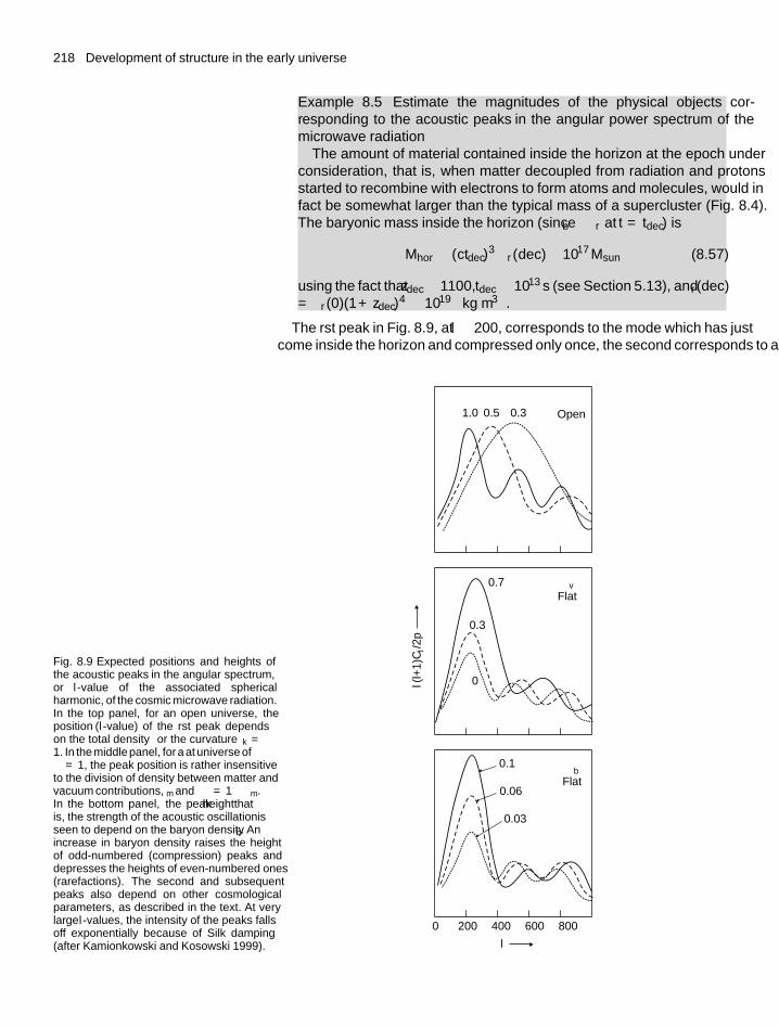
218 Development of structure in the early universe
Example 8.5 Estimate the magnitudes of the physical objects cor-responding to the ‘acoustic peaks’ in the angular power spectrum of themicrowave radiation
The amount of material contained inside the horizon at the epoch underconsideration, that is, when matter decoupled from radiation and protonsstarted to recombine with electrons to form atoms and molecules, would infact be somewhat larger than the typical mass of a supercluster (Fig. 8.4).The baryonic mass inside the horizon (since ρb ∼ ρr at t = tdec) is
Mhor ∼ (ctdec)3 ρr(dec) ∼ 1017 Msun (8.57)
using the fact that zdec ∼ 1100, tdec ∼ 1013 s (see Section 5.13), and ρr(dec)= ρr(0)(1 + zdec)
4 ∼ 10−19 kg m−3.
The first peak in Fig. 8.9, at l ∼ 200, corresponds to the mode which has justcome inside the horizon and compressed only once, the second corresponds to a
Fig. 8.9 Expected positions and heights ofthe ‘acoustic peaks’ in the angular spectrum,or l-value of the associated sphericalharmonic, of the cosmic microwave radiation.In the top panel, for an open universe, theposition (l-value) of the first peak dependson the total density � or the curvature �k =1−�. In the middle panel, for a flat universe of� = 1, the peak position is rather insensitiveto the division of density between matter andvacuum contributions, �m and �� = 1−�m.In the bottom panel, the peak height—thatis, the strength of the acoustic oscillation—isseen to depend on the baryon density �b. Anincrease in baryon density raises the heightof odd-numbered (compression) peaks anddepresses the heights of even-numbered ones(rarefactions). The second and subsequentpeaks also depend on other cosmologicalparameters, as described in the text. At verylarge l-values, the intensity of the peaks fallsoff exponentially because of Silk damping(after Kamionkowski and Kosowski 1999).
0.1
0.06
0.03
0.7
0.3
0
0.51.0 0.3
ΩvFlat
ΩOpen
ΩbFlat
l(l+
1)C
l/2p
200 400 600 8000
l
8.14 Angular spectrum of anisotropies: ‘acoustic peaks’ 219
shorter wavelength mode which has undergone rarefaction, and so on. For muchlower values of l and angles above a few degrees, the temperature variationsare dominated by the SW effect described in a previous section. Because theordinate factor l(l + 1) ∼ k2 or 1/λ2 cancels the λ2 dependence in (8.29), thislarge-angle part of the plot should be fairly flat (the so-called SW plateau). Thisresult follows basically from scale invariance predicted in the inflation scenarioand assumed in deriving (8.29).
8.14.1 Peak position versus density parameters
First we consider the case of an open matter-dominated universe with zerocosmological constant (i.e. �� = 0) at z-values where the radiation term isstill comparatively small (i.e. z < 1000). The true coordinate distance todayof an object at redshift z is D(z), as given in the second of equations (5.44), sothat with �k = (1 − �m) and �� = �r = 0 we get from (5.43):
I(z) =z∫
0
dz[�m (1 + z)3 + (1 − �m) (1 + z)2]1/2
=∫
dz[(1+z) (1 + �mz)1/2
](8.58)
This integration can be performed by making the substitution (1 + �mz) =(1 − �m) sec2θ, when it has the value
I(z) =[(1 − �m)−1/2
]ln
[(1 + cos θ)
(1 − cos θ)
]=(
1
q
)ln
[ {(p + q)(1 − q)}{p − q)(1 + q)}
]where p2 = (1 + �mz), q2 = (1 − �m) = �k . With sinh X = (eX − e−X )/2the middle equation (5.44b) then gives the following expression for the distancetoday of an object at redshift z:
D(z) = R(0)r =[
c
H0 (1 − �m)1/2
]sinh
{ln
[(p + q
) (1 − q
)(p − q
) (1 + q
)]}
=(
2c
H0
) [�mz − (2 − �m){(1 + �mz)1/2 − 1
}][�2
m(1 + z)]
(8.59)
known as the Mattig formula, valid, we repeat, for an open, matter-dominateduniverse with zero vacuum energy and the radiation contribution neglected.
For a very distant object at high redshift z, (8.59) gives the simpleapproximate result, actually independent of the z-value, provided it is large:
D(z) ≈ 2c
(H0�m)(8.60)
We note that for �m = 1, this is just the expression for the optical horizondistance in a flat, matter-dominated universe. So the effect of an open matter-dominated universe is just to enlarge the horizon by a factor 1/�m.
220 Development of structure in the early universe
The second important case is that of a flat universe, with the dominantcontributions from matter and from vacuum energy, that is, with �� = 1−�m
and �k = �r = 0. In this case the integral (5.43) has the form
I(z) =∫
dz[�m (1 + z)3 + (1 − �m)
]1/2(8.61)
No analytical solution is possible and the integration has to be performednumerically. However, for values of z > 4 and �m > 0.05 one can neglect thevacuum term in comparison with the matter term and perform that part of theintegral analytically, so that only a few minutes’ work with a pocket calculatoris needed to plot D versus � for a fixed z. We discuss the results below.
We now consider the value of the angle subtended today at the Earth bythe acoustic horizon at the time of last scattering of the CMB (t = tdec). Asshown in Section 5.13, matter and photon energy densities would actually havebeen equal at the larger value, zeq ∼ 5000. But first let us assume radiationdominance for z > zdec, the epoch of last scattering. Since the curvature term isnegligible in comparison with the radiation and matter terms at large z-values,distances are given by the flat universe formula in (5.44b). The ratio of sound tolight velocity in a situation where radiation is prominent is 1/
√3 (see Table 5.2).
Hence, integrating from z = zdec to z = ∞, the acoustic horizon distance atthe time of last scattering of the radiation is now
DH ≈(
c
H0
)∫dz[
(3�r)1/2 (1 + z)2] = c[
H0 (1 + zdec) (3�r)1/2] (8.62)
In our very crude approximation, �r(0) ∼ �m(0)/(1 + zdec), so this result canalso be written
DH ≈ c[H0{(1 + zdec) 3�m
}1/2] (8.63)
Had we instead assumed matter dominance for most of the range z = zdec toz = ∞, we would have obtained exactly twice this value. If we now divide byD(z) in (8.60), we obtain the value of the angle θ now subtended by the acoustichorizon at z = zdec. This therefore indicates the position of the first acousticpeak, with angle given by
θ√�m
∼ [3 (1 + z)]−1/2 ∼ 1◦ (8.64)
in agreement with our first estimate (8.54). This result applies for the case ofan open matter-dominated universe with no vacuum energy term. It is based onseveral simplifying assumptions and the absolute value of the angle is thereforeonly approximate, but the result gives a feeling for the magnitudes and principalfactors involved. In any case, the main result stands, namely that the anglesubtended varies as �
1/2m . For the flat universe case, the angle has to be found
by numerical integration. The results are discussed below.As indicated by (8.64), the position (angle or l-value) of the first peak
depends on the value of the curvature parameter k, or more specifically
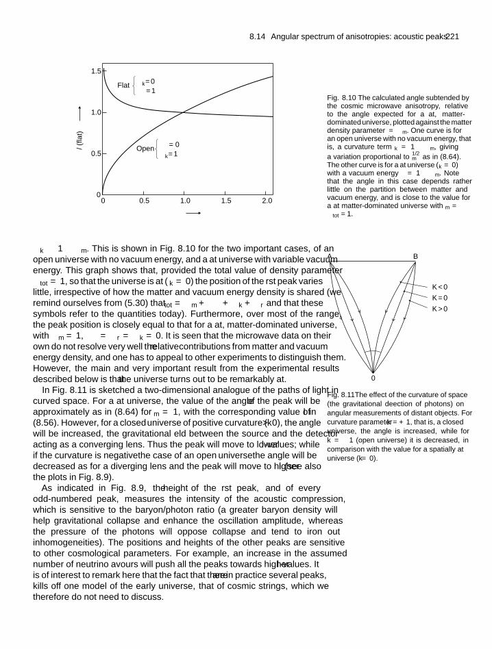
8.14 Angular spectrum of anisotropies: ‘acoustic peaks’ 221
Ω
Ωk = 0Ω�= 1– Ω
Flat�/
� (f
lat)
Ω�= 0Ωk = 1– Ω
Open
1.5
1.0
0.5
01.51.00.50 2.0
Fig. 8.10 The calculated angle subtended bythe cosmic microwave anisotropy, relativeto the angle expected for a flat, matter-dominated universe, plotted against the matterdensity parameter � = �m. One curve is foran open universe with no vacuum energy, thatis, a curvature term �k = 1 − �m, givinga variation proportional to �
1/2m as in (8.64).
The other curve is for a flat universe (�k = 0)with a vacuum energy �λ = 1 − �m. Notethat the angle in this case depends ratherlittle on the partition between matter andvacuum energy, and is close to the value fora flat matter-dominated universe with �m =�tot = 1.
�k ≡ 1 − �m. This is shown in Fig. 8.10 for the two important cases, of anopen universe with no vacuum energy, and a flat universe with variable vacuumenergy. This graph shows that, provided the total value of density parameter�tot = 1, so that the universe is flat (�k = 0) the position of the first peak varieslittle, irrespective of how the matter and vacuum energy density is shared (weremind ourselves from (5.30) that �tot = �m + �� + �k + �r and that thesesymbols refer to the quantities today). Furthermore, over most of the range,the peak position is closely equal to that for a flat, matter-dominated universe,with �m = 1, �� = �r = �k = 0. It is seen that the microwave data on theirown do not resolve very well the relative contributions from matter and vacuumenergy density, and one has to appeal to other experiments to distinguish them.However, the main and very important result from the experimental resultsdescribed below is that the universe turns out to be remarkably flat. 0
A B
K = 0
K < 0
K > 0
Fig. 8.11 The effect of the curvature of space(the gravitational deflection of photons) onangular measurements of distant objects. Forcurvature parameter k = +1, that is, a closeduniverse, the angle is increased, while fork = −1 (open universe) it is decreased, incomparison with the value for a spatially flatuniverse (k = 0).
In Fig. 8.11 is sketched a two-dimensional analogue of the paths of light incurved space. For a flat universe, the value of the angle θ of the peak will beapproximately as in (8.64) for �m = 1, with the corresponding value of l in(8.56). However, for a ‘closed’universe of positive curvature (k > 0), the anglewill be increased, the gravitational field between the source and the detectoracting as a converging lens. Thus the peak will move to lower l-values; whileif the curvature is negative—the case of an ‘open’ universe—the angle will bedecreased as for a diverging lens and the peak will move to higher l (see alsothe plots in Fig. 8.9).
As indicated in Fig. 8.9, the height of the first peak, and of everyodd-numbered peak, measures the intensity of the acoustic compression,which is sensitive to the baryon/photon ratio (a greater baryon density willhelp gravitational collapse and enhance the oscillation amplitude, whereasthe pressure of the photons will oppose collapse and tend to iron outinhomogeneities). The positions and heights of the other peaks are sensitiveto other cosmological parameters. For example, an increase in the assumednumber of neutrino flavours will push all the peaks towards higher l-values. Itis of interest to remark here that the fact that there are in practice several peaks,kills off one model of the early universe, that of ‘cosmic strings’, which wetherefore do not need to discuss.
222 Development of structure in the early universe
8.15 Experimental observation andinterpretation of CMB anisotropies
The design of experiments to detect the tiny anisotropies of order 10−5 in theCMB has been a very challenging problem. Because water vapour absorbsmicrowave radiation, the detectors have been mounted on satellites (the COBEand WMAP experiments), or flown on balloons at high and dry locations, suchas the South Pole. The instruments themselves employ cryogenic cooling toreduce background, and bolometer or superconducting detectors, and may alsobe operated as interferometers measuring directly the tiny spatial variations intemperature. Ubiquitous background, such as infrared emission from the MilkyWay, has been eliminated by means of suitable combinations of frequencies. Thesuccess of these experiments in digging out the tiny signals from the backgroundhas to be regarded as one of the great triumphs of modern experimental physics.
As mentioned above, the first crucial detection of anisotropies (the existenceof which had been predicted some 30 years previously) at the 10−5 level wasachieved by the differential microwave radiometer on the COBE satellite in1992 (Smoot et al. 1992, Bennett et al. 1996, Mather et al. 2000), with, however,an angular resolution of only about 7◦. Since then, measurements have beencarried out with detectors having much higher angular resolution—typically10′–50′ of arc. Some were flown on high altitude balloons—the BOOMERANG(de Bernardis et al. 2002) and MAXIMA (Lee et al. 2001) experiments—andone was a ground-based interferometer—the DASI (Halverson et al. 2001)experiment—all at the South Pole. The most detailed data to date have beenobtained with WMAP, the Wilkinson Microwave Anisotropy Probe satelliteexperiment (Bennett et al. 2003, Spergel et al. 2003). Over a six month periodof observation, this was able to cover the entire sky. Observations were madewith cooled differential radiometers at five frequency bands, ranging from 23 to94 GHz. These variations in temperature on small scales have provided our bestinformation on the parameters of the early universe, such as the curvature andthe contributions of matter, radiation, and vacuum terms to the overall energydensity.
Figure 8.12 shows the angular spectrum with its acoustic peaks in the WMAPand other experiments. The best fit to this data corresponds to the cosmicparameters shown in Table 8.1 below. There is clear evidence for a third peak,but at higher and higher l-values, the amplitude falls off exponentially becauseof the increasing effects of photon damping of the density fluctuations at shortdistances, as described in Section 8.13 above.
The microwave photons have primary anisotropies which correspond to theirdistribution upon leaving the ‘last scattering surface’ at the time of decouplingat zdec = 1100. In fact, this is a last scattering ‘shell’ rather than a surface,with a thickness which is obviously of the order of the photon mean free pathbetween Thomson scatters. If the medium were fully ionized, this is readilycalculated to be ∼2 kpc at that time, but would be considerably more than this,since the degree of ionization was varying rapidly at z = zdec (recall the Sahaequation in Chapter 5). So the photons last scatter over a small range of z-values(typically �z ∼ 60) and this and the effects of secondary anisotropies meanthat any angular variations below about 0.03◦ would be completely smearedout and undetectable (see Problem 8.9).
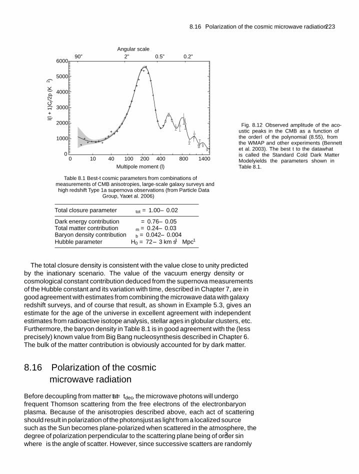
8.16 Polarization of the cosmic microwave radiation 223
600090º 2º 0.5º 0.2º
5000
4000
3000
2000
l(l +
1)C
l/2p
(�
K2 )
1000
00 40 100 200
Multipole moment (l)
Angular scale
400 800 140010
Fig. 8.12 Observed amplitude of the ‘aco-ustic peaks’ in the CMB as a function ofthe order l of the polynomial (8.55), fromthe WMAP and other experiments (Bennettet al. 2003). The best fit to the data—whatis called the ‘Standard Cold Dark MatterModel’—yields the parameters shown inTable 8.1.
Table 8.1 Best-fit cosmic parameters from combinations ofmeasurements of CMB anisotropies, large-scale galaxy surveys andhigh redshift Type 1a supernova observations (from Particle Data
Group, Yao et al. 2006)
Total closure parameter �tot = 1.00 ± 0.02
Dark energy contribution �� = 0.76 ± 0.05Total matter contribution �m = 0.24 ± 0.03Baryon density contribution �b = 0.042 ± 0.004Hubble parameter H0 = 72 ± 3 km s−1 Mpc−1
The total closure density is consistent with the value close to unity predictedby the inflationary scenario. The value of the vacuum energy density orcosmological constant contribution deduced from the supernova measurementsof the Hubble constant and its variation with time, described in Chapter 7, are ingood agreement with estimates from combining the microwave data with galaxyredshift surveys, and of course that result, as shown in Example 5.3, gives anestimate for the age of the universe in excellent agreement with independentestimates from radioactive isotope analysis, stellar ages in globular clusters, etc.Furthermore, the baryon density in Table 8.1 is in good agreement with the (lessprecisely) known value from Big Bang nucleosynthesis described in Chapter 6.The bulk of the matter contribution is obviously accounted for by dark matter.
8.16 Polarization of the cosmicmicrowave radiation
Before decoupling from matter at t = tdec, the microwave photons will undergofrequent Thomson scattering from the free electrons of the electron–baryonplasma. Because of the anisotropies described above, each act of scatteringshould result in polarization of the photons—just as light from a localized sourcesuch as the Sun becomes plane-polarized when scattered in the atmosphere, thedegree of polarization perpendicular to the scattering plane being of order sin2θ
where θ is the angle of scatter. However, since successive scatters are randomly
224 Development of structure in the early universe
orientated, all polarization effects will be washed out, except for that arising inthe very last act of scattering before the decoupling time, tdec. The direction ofthis polarization will vary with the angle of observation, depending on the spatialanisotropies involved. Such polarization has been measured with the DASIinterferometer and more recently by the WMAP experiment, and is exactlyof the magnitude (a few μK) expected. In addition to these effects at smallangles of observation (but of course primarily due to large angles of scatter)polarization due to secondary processes discussed in Section 8.13.2 above, willbe observed at large angles, in the region of the SW plateau, and as alreadydescribed, has given information on the re-ionization of the interstellar medium.
The polarization produced in Thomson scattering is of the so-called E-mode.In general, polarization has to be described by a second-rank tensor, andcan also exist in the so-called B-mode. The distinction between the two isthat, if one decomposes the angular dependence into spherical harmonics, E-mode polarization has parity (−1)l while B-mode has parity (-1)l+1. A vectorinteraction such as Thomson scattering cannot produce the B-mode, whichrequires a tensor interaction, such as that of gravity waves.
The amount of B-mode polarization due to the burst of gravitational radiationwhich is expected to accompany inflation, is calculated to be associated withtemperature fluctuations at best at the level of 0.1 μK and will therefore be verydifficult to detect. It is one of the primary aims of the future Planck satelliteexperiment to be launched by the European Space Agency. Of course, with theCMB photons we cannot look directly back before the time of matter–radiationdecoupling. However, gravitational waves can be directly associated with theinflation process, and can leave their imprint on the microwave background inthe form of polarization anisotropies. This seems to offer the only real hope ofexamining the details of the inflation process at very much earlier times, and iscertainly one of the most important future goals of cosmological research.
8.17 Summary
• The conventional Big Bang model, while successfully accounting for theredshift, abundance of light elements, and the microwave backgroundradiation, suffers from the horizon and flatness problems.
• The horizon problem arises on account of the observed isotropy of themicrowave background out to the largest angles. The horizon at thetime of the decoupling of matter and radiation, at z ∼ 1000 (when theradiation had the last opportunity of interaction and achieving thermalequilibrium), now only subtends about 1◦ at the Earth. It is thereforeimpossible to understand how the large-angle uniformity in temperaturecould have been achieved by causal processes.
• The flatness problem arises because the fractional difference between theobserved density ρ and the critical density ρc should be proportional to tin a radiation-dominated universe, and t4/3 in the matter-dominated case.Thus at very early times, ρ must have been very finely tuned to ρc (to anaccuracy of only one part in 1052, if we go back to the Planck era).
• The postulate of a preliminary inflationary stage of exponentialexpansion, when the radius of the initial micro-universe expanded from10−26 m to 1 m, solves both these problems, and also accounts for theabsence of magnetic monopoles.
8.17 Summary 225
• Quantum fluctuations at the commencement of inflation may account forthe observed perturbations, of order 10−5, in the temperature (and hencedensity) of the cosmic microwave radiation. These quantum fluctuationswould become classical, frozen fluctuations in density when they wereinflated beyond the causal horizon.
• Large-scale structures in the universe—galaxies, galaxy clusters, voids,etc.—were seeded by these primordial perturbations in the density (ormetric curvature).
• Initially, the density perturbations δ = �ρ/ρ grew linearly with theexpansion parameter R as they collapsed under gravity in the era of matterdomination. The collapse became possible on all scales larger than theJeans length, in turn determined by the speed of sound vs in the cosmicfluid. As vs decreased abruptly when atoms began to form, more dramatic,and non-linear, collapse on smaller and smaller scales became possible.
• The spectrum of density fluctuations predicted by inflation is a power law,with no preferred scale, and (�ρ/ρ)rms ∼ λ−2, where λ is the lengthinvolved. The spectrum observed in COBE microwave measurementsat large angular scales fits this prediction. At smaller scales, below400 Mpc, the fluctuation spectrum from galaxy surveys is much flatter,due to damping of the density perturbations by photon diffusion andcollisionless damping by the relic neutrino component, and is consistentwith expectations from mixed dark matter models. The degree of dampinghas been used to set limits of less than 0.4 eV/c2 on the neutrino mass,summed over the three neutrino flavours.
• The tiny (10−5) variations in the observed microwave temperaturebetween pairs of points in the sky separated by angle θ can be describedby a sum of Legendre polynomials Pl(cos θ), where l-values of 100–1000are relevant to investigations at separation angles of the order 1◦ or less.The amplitudes of these fluctuations in temperature, consequent on thedensity fluctuations, appear as a series of so-called ‘acoustic peaks’whenplotted against the l-value.
• The position of the first acoustic peak, at l ≈ 200, provides a measure ofthe total density parameter �tot, indicating a value close to unity, and aconsequent curvature parameter �k = 1 − � of less than 0.05: thus theearly universe is practically flat, as predicted by the inflation model. Theheight of the first peak and the heights and positions of the other peaksprovide estimates for other cosmological parameters, such as the baryondensity, the amount of dark matter, Hubble parameter, etc., and whencombined with data from galaxy surveys and high redshift supernova,provide the basic parameters describing the universe.
• The CMB is found to be polarized, due to Thomson scattering from freeelectrons, either in a final act of scattering before decoupling at z ∼ 1000,or later, en route through an intergalactic medium re-ionized by ultravioletlight emitted by the early stars. One also expects a separate polarizationdue to tensor interactions of gravitational waves accompanying inflation,and this will constitute an important test of the inflation hypothesis,hopefully to be observed by the future Planck satellite mission.
226 Development of structure in the early universe
Problems
More challenging problems are denoted with an asterisk.
(8.1) Show that the free-fall time (8.34) is of the same orderof magnitude as the period of a satellite in close orbitabout a spherical cloud of density ρ.
(8.2) Calculate the Jeans mass and Jeans length for a massof air at NTP (T = 273 K, ρ = 1.29 kg m−3).
(8.3) Verify the expressions (8.42)–(8.44) for the growth ofthe density contrast with time in a closed (k = +1)matter-dominated universe. Derive the correspondingexpressions for an open universe, with k = −1, andshow that in this case the density contrast will decreasewith time.
(8.4) Assume that a density fluctuation occurs during theinflation process, and that at the end of inflation, atti ∼ 10−32 s, this has become ‘frozen-out’ at a lengthscale λ, when the universe has reached a radius ∼ 1m. Calculate at what subsequent time the perturbationwill come inside the horizon and start to oscillate asan ‘acoustic’ wave, for λ = 1 mm and for λ = 1 cm.Estimate the masses inside the horizon in the two casesand identify them with large-scale structures.
(8.5) Calculate the Jeans length at time t in the early,radiation-dominated universe, and show that it isapproximately equal to the horizon distance at thattime.
(8.6) Starting from the formula (5.44), calculate the presentdistance to the optical horizon DH for the case of aflat universe (k = 0) with �m = 0.24 and �� =0.76, neglecting the contribution of radiation. (A short
numerical integration will be needed for z < 4.For larger z values the vacuum contribution can beneglected, and the integral evaluated analytically.)
*(8.7) Find an expression for the probability that microwavephotons observed today will have undergone Thomsonscattering due to re-ionization of the intergalacticmedium (by ultraviolet light from the first stars), asa function of the value of the redshift below which re-ionization is assumed to take place. If this probability is10%, find below which value of z the medium is almosttotally ionized, and at what time after the Big Bang thisoccurs. Assume that the universe has matter energydensity with �m = 0.26 and baryon density �b =0.045, and for simplicity suppose that for the z-valuesinvolved, radiation, vacuum energy, and curvature canall be neglected (i.e. �r = �� = �k = 0).
(8.8) Estimate the escape velocities from a typical galaxyand from a typical galaxy cluster. Compare this withthe mean velocity of relic neutrinos, assuming that theyare non-relativistic with a Maxwellian distribution invelocity, and have masses of 0.1, 1.0, or 10 eV/c2.
*(8.9) Calculate the mean path length between Thomsonscatters of the CMB photons at z ∼ zdec = 1100,assuming the medium to be completely ionized.Because the appropriate degree of ionization near thepoint of decoupling is small, assume the thicknessof the ‘last scattering shell’ is 10 times this length.Calculate the corresponding variation in �z and theresultant angular smearing of the acoustic peaks in theangular spectrum of the radiation. (Hint: refer to (8.64)and to (5.43) and (5.44), assuming a flat universe).
Part 3
Particles and Radiationin the Cosmos

This page intentionally left blank
Cosmic particles 99.1 Preamble
The particles circulating in the cosmos include the so-called cosmic rays,which have been intensively studied ever since their discovery by Hess in1912. Karl K. Darrow, a past chairman of the American Physical Society,caught some of the atmosphere of this early research when he described theirstudy as remarkable ‘for the delicacy of the apparatus, the minuteness of thephenomena, the adventurous excursions of the experimenters and the grandeurof the inferences’.
Cosmic rays consist of high-energy particles incident on the Earth from outerspace, plus the secondary particles which they generate as they traverse theatmosphere. Their study has a special place in physics, not only in its own right,but because of the pioneering role that cosmic ray research has played—andis still playing—in the study of elementary particles and their interactions. Wecan recall the discovery in cosmic rays of antimatter, in the form of the positronand e+e− pair production in 1932, and of pions and muons and strange particlesin the late 1940s. In those days, before 1950, the cosmic radiation was the onlyavailable source of high-energy particles (those above about 1 GeV). Thesediscoveries indeed kick-started the building of large particle accelerators andthe development of their associated detecting equipment, developments whichwere essential in broadening the scope of the subject and putting elementaryparticle physics on a sound quantitative basis.
Later, in the 1980s and 1990s, the study of the interactions of solar andatmospheric neutrinos, on distance scales far larger than anything that had beenattempted at accelerators or reactors, revealed the first cracks in the StandardModel, with evidence for neutrino flavour mixing and for finite neutrinomasses, as described in Section 4.2 and Sections 9.15–9.17. This has led toa revival, in the new millennium, of lepton physics in fixed-target experimentsat accelerators, and to the development of radically new proposals such as thebuilding of muon storage rings to serve as sources of high-energy electron– andmuon–neutrinos.
At the highest energies, study of γ-rays in the TeV range and above hasindicated point sources in the skies where it seems the most violent eventsin the universe have taken place, and intensive studies of both γ-rays andultra-high-energy protons and heavier nuclei will certainly shed new lighton mechanisms for particle acceleration, as well perhaps as revealing newfundamental processes taking place at energies far in excess of what could everbe achieved on the Earth. The study of cosmic rays is indeed still a very openfield, where new developments and mysteries arise on an almost daily basis.
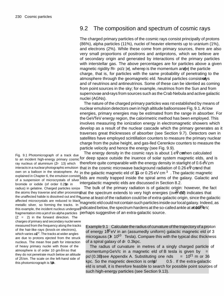
230 Cosmic particles
9.2 The composition and spectrum of cosmic rays
The charged primary particles of the cosmic rays consist principally of protons(86%), alpha particles (11%), nuclei of heavier elements up to uranium (1%),and electrons (2%). While these come from primary sources, there are alsovery small proportions of positrons and antiprotons, which we believe areof secondary origin and generated by interactions of the primary particleswith interstellar gas. The above percentages are for particles above a givenmagnetic rigidity R = pc/z |e|, where p is the momentum and z|e| the particlecharge, that is, for particles with the same probability of penetrating to theatmosphere through the geomagnetic field. Neutral particles consist of γ-raysand of neutrinos and antineutrinos. Some of these can be identified as comingfrom ‘point’ sources in the sky; for example, neutrinos from the Sun and fromsupernovae and γ-rays from sources such as the Crab Nebula and active galacticnuclei (AGNs).
The nature of the charged primary particles was first established by means ofnuclear emulsion detectors flown in high altitude balloons—see Fig. 9.1. At lowenergies, primary energies may be estimated from the range in absorber. Forthe GeV–TeV energy region, the calorimetric method has been employed. Thisinvolves measuring the ionization energy in electromagnetic showers whichdevelop as a result of the nuclear cascade which the primary generates as ittraverses great thicknesses of absorber (see Section 9.7). Detectors flown insatellites have employed scintillation counters to measure the primary nuclearcharge from the pulse height, and gas-filled Cerenkov counters to measure theparticle velocity and hence the energy (see Fig. 9.9).
Fig. 9.1 Photomicrograph of a track dueto an incident high-energy primary cosmicray nucleus of aluminium (Z = 13) whichinteracts in a ‘nuclear’photographic emulsionflown on a balloon in the stratosphere. Asexplained in Chapter 6, the emulsion consistsof a suspension of microcrystals of silverbromide or iodide (of order 0.25 μm inradius) in gelatine. Charged particles ionizethe atoms they traverse and after processing,the unaffected halide is dissolved out and theaffected microcrystals are reduced to blackmetallic silver, so forming the tracks. Inthis example, the incident nucleus undergoesfragmentation into a ‘jet’of six alpha particles(Z = 2) in the forward direction. Thecharges of primary and secondary nuclei weremeasured from the frequency along the tracksof the hair-like δ-rays (knock-on electrons),which varies as Z2. The tracks at wider anglesare due to protons ejected from the strucknucleus. The mean free path for interactionof heavy primary nuclei with those of theatmosphere is of order 10 gm cm−2 so thatthey do not penetrate much below an altitudeof 25 km. The scale on the left-hand side ofthis photomicrograph is 50 μm.
The energy density in the cosmic rays is about 1 eV cm−3 when calculatedfor deep space outside the influence of solar system magnetic fields, and istherefore quite comparable with the energy density in starlight of 0.6 eV cm−3,that in the cosmic microwave background radiation of 0.26 eV cm−3, and thatin the galactic magnetic field of 3 μG or 0.25 eV cm−3. The galactic magneticfields are mostly trapped inside the spiral arms of the galaxy. Galactic andintergalactic magnetic fields are discussed in Section 8.2.
The bulk of the primary radiation is of galactic origin: however, the factthat the spectrum extends to very high energies (over 1020 eV) indicates thatsome at least of the radiation could be of extra-galactic origin, since the galacticmagnetic field could not contain such particles inside our local galaxy. Indeed, asindicated below, the spectrum hardens at the so-called ankle at about 4×10¹⁸ eV,perhaps suggestive of an extra-galactic source.
Example 9.1 Calculate the radius of curvature of the trajectory of a protonof energy 1020 eV in an (assumedly uniform) galactic magnetic field of 3microgauss (3 × 10⁻¹⁰ Tesla). Compare this with the typical disc thicknessof a spiral galaxy of d = 0.3 kpc.
The radius of curvature ρ in metres of a singly charged particle ofmomentum p GeV/c in a magnetic field of B tesla is given by ρ =pc/(0.3B)—see Appendix A. Substituting one finds ρ = 1021 m or 36kpc. So the magnetic deflection is only d/ρ ∼ 0.5◦. If the extra-galacticfield is small, it is therefore feasible to search for possible point sources ofsuch high-energy particles (see Section 9.13).
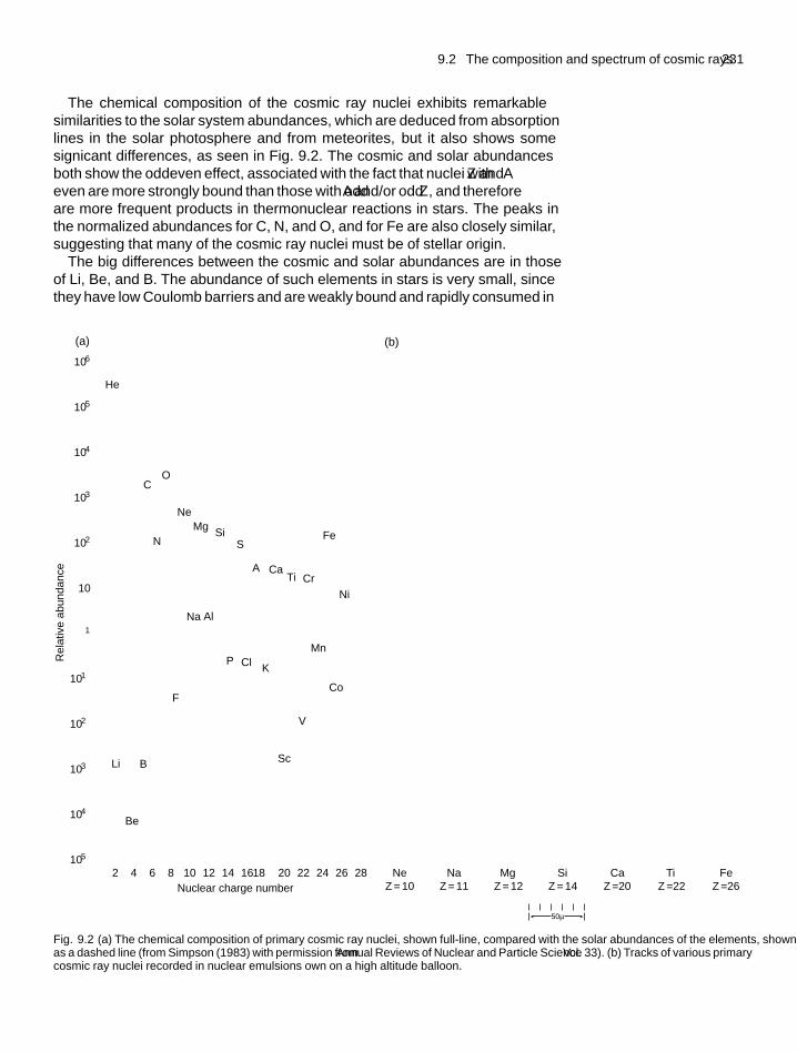
9.2 The composition and spectrum of cosmic rays 231
The chemical composition of the cosmic ray nuclei exhibits remarkablesimilarities to the solar system abundances, which are deduced from absorptionlines in the solar photosphere and from meteorites, but it also shows somesignificant differences, as seen in Fig. 9.2. The cosmic and solar abundancesboth show the odd–even effect, associated with the fact that nuclei with Z and Aeven are more strongly bound than those with odd A and/or odd Z , and thereforeare more frequent products in thermonuclear reactions in stars. The peaks inthe normalized abundances for C, N, and O, and for Fe are also closely similar,suggesting that many of the cosmic ray nuclei must be of stellar origin.
The big differences between the cosmic and solar abundances are in thoseof Li, Be, and B. The abundance of such elements in stars is very small, sincethey have low Coulomb barriers and are weakly bound and rapidly consumed in
106
105
104
103
102
10
1
10–1
10–2
10–3
10–4
10–5
2 4 6 8 10 12 14 16 20 22 24 26 2818Nuclear charge number
Rel
ativ
e ab
unda
nce
He
C
N
Ne
Fe
Cr
Ni
TiCa
Co
A
Mg
AlNa
F
BLi
Be
K
Sc
V
ClMn
P
SiS
O
NeZ = 10
NaZ = 11
MgZ = 12
SiZ = 14
50μ
CaZ =20
TiZ =22
FeZ =26
(a) (b)
Fig. 9.2 (a) The chemical composition of primary cosmic ray nuclei, shown full-line, compared with the solar abundances of the elements, shownas a dashed line (from Simpson (1983) with permission from Annual Reviews of Nuclear and Particle Science Vol. 33). (b) Tracks of various primarycosmic ray nuclei recorded in nuclear emulsions flown on a high altitude balloon.
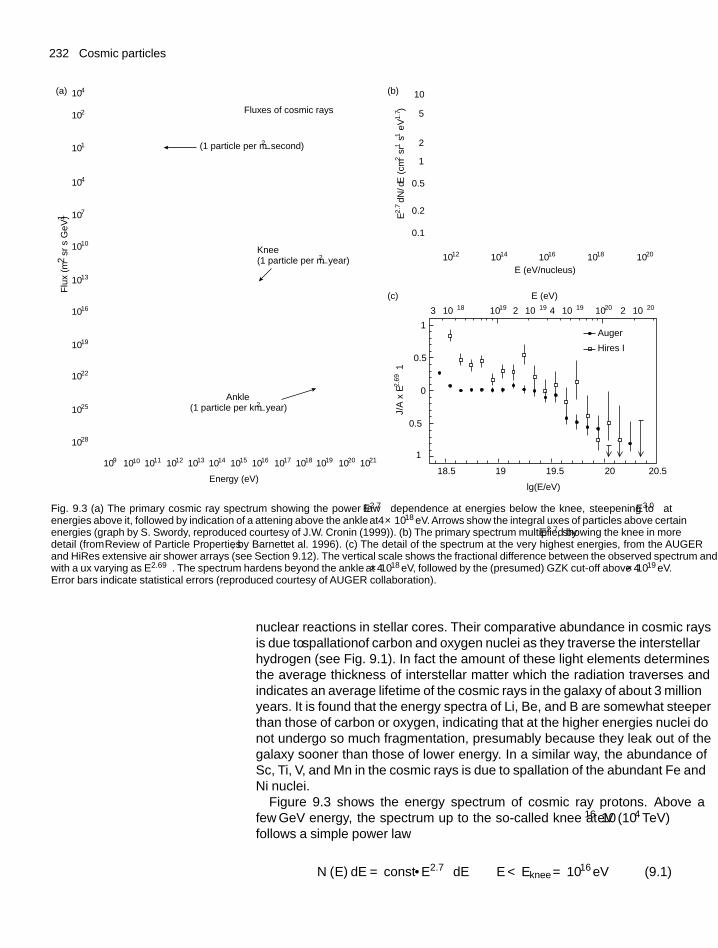
232 Cosmic particles
3 1018
1
0.5
J/A
x E
–2.6
9–1
–0.5
18.5 19 19.5 20
Auger
Hires I
lg(E/eV)
20.5
–1
0
2 1019
E (eV)
4 1019 2 102010201019
104
102
10–1
10–4
10–7
10–10
10–13
10–16
10–19
10–22
10–25
10–28
Energy (eV)
109
1012 1014 1016
E (eV/nucleus)
E2.
7dN
/dE
(cm
–2sr
–1s–1
eV1.
7 )
1018 1020
10
5
2
1
0.5
0.2
0.1
1010 1011 1012 1013 1014 1015 1016 1017 1018 1019 1020 1021
Ankle(1 particle per km2_ year)
(a) (b)
(c)
(1 particle per m2_ second)
Fluxes of cosmic rays
Flux
(m
2 sr
s G
eV)–
1
Knee(1 particle per m2_ year)
Fig. 9.3 (a) The primary cosmic ray spectrum showing the power law E−2.7 dependence at energies below the ‘knee’, steepening to E−3.0 atenergies above it, followed by indication of a flattening above the ‘ankle’ at ∼ 4×10¹⁸ eV. Arrows show the integral fluxes of particles above certainenergies (graph by S. Swordy, reproduced courtesy of J.W. Cronin (1999)). (b) The primary spectrum multiplied by E2.7, showing the knee in moredetail (from Review of Particle Properties, by Barnett et al. 1996). (c) The detail of the spectrum at the very highest energies, from the AUGERand HiRes extensive air shower arrays (see Section 9.12). The vertical scale shows the fractional difference between the observed spectrum and onewith a flux varying as E−2.69. The spectrum hardens beyond the ‘ankle’ at 4 × 10¹⁸ eV, followed by the (presumed) GZK cut-off above 4 × 10¹⁹ eV.Error bars indicate statistical errors (reproduced courtesy of AUGER collaboration).
nuclear reactions in stellar cores. Their comparative abundance in cosmic raysis due to spallation of carbon and oxygen nuclei as they traverse the interstellarhydrogen (see Fig. 9.1). In fact the amount of these light elements determinesthe average thickness of interstellar matter which the radiation traverses andindicates an average lifetime of the cosmic rays in the galaxy of about 3 millionyears. It is found that the energy spectra of Li, Be, and B are somewhat steeperthan those of carbon or oxygen, indicating that at the higher energies nuclei donot undergo so much fragmentation, presumably because they leak out of thegalaxy sooner than those of lower energy. In a similar way, the abundance ofSc, Ti, V, and Mn in the cosmic rays is due to spallation of the abundant Fe andNi nuclei.
Figure 9.3 shows the energy spectrum of cosmic ray protons. Above afew GeV energy, the spectrum up to the so-called knee at 1016 eV (104 TeV)follows a simple power law
N (E) dE = const · E−2.7 dE E < Eknee = 1016 eV (9.1)
9.3 Geomagnetic and solar effects 233
Above this ‘knee’the spectrum becomes steeper with an index of approximately−3.0
N (E) dE = const · E−3.0 dE Eankle > E > Eknee (9.2a)
before hardening again above the so-called ankle at Eankle ≈ 4 × 10¹⁸ eV:
N (E) dE = const · E−2.69 dE EGZK > E > Eankle (9.2b)
Above EGZK = 4 × 10¹⁹ eV, the spectra found by extensive air showerexperiments—theAUGER experiment inArgentina and the HiRes (‘Fly’s Eye’)detector in Utah—appear to fall off, presumably because of the ‘GZK cut-off’due to pion production in collisions with the microwave background photons(see Section 9.12). They are parameterized by the form
N (E) dE = const · E−4.2 dE E > EGZK = 4 × 10¹⁹ eV (9.2c)
From the development of the air showers as a function of atmospheric depth,it is known that over the entire energy ranges above, the primary particles areboth protons and heavier nuclei.
At energies above 30 GeV, where effects due to the magnetic fields of theEarth or the Sun are unimportant, the radiation appears to be isotropic, since thegalactic magnetic fields would destroy any initial anisotropy except at extremelyhigh energies. Data from the AUGER air shower experiment does detectanisotropies and close and significant correlations of showers above 6×10¹⁹ eVwith known AGNs within about 75 Mpc of the Earth (see Section 9.13).
9.3 Geomagnetic and solar effects
The primary radiation, for charged particles below 10 GeV energy, does showdirectional effects and also time dependence. The charged primaries are affectedby the Earth’s magnetic field, which approximates that due to a simple magneticdipole, and also by modulation in time due to the solar wind, which follows the11-year solar cycle.
We first discuss the geomagnetic effects. The axis of the dipole is at an angleto the axis of the Earth’s rotation. The geographical coordinates of the polesvaries slowly with geological time, the present N pole being located at longitude101◦ W, latitude 75◦ N. The calculation of the actual orbits of particles incidenton the Earth as they spiral in the dipole field is rather tedious and complex, andmost easily accomplished using a computer program. However, some of themain features of the geomagnetic effects can be understood analytically.
Consider first a particle of charge z|e|, velocity v, and momentum p = mvtravelling in a circular equatorial path of radius r around a short dipole ofmoment M . Equating centrifugal and magnetic forces we obtain
z |e| |B × v| = mv2
r
where the equatorial field due to the dipole is
B =(μ0
4π
) M
r3
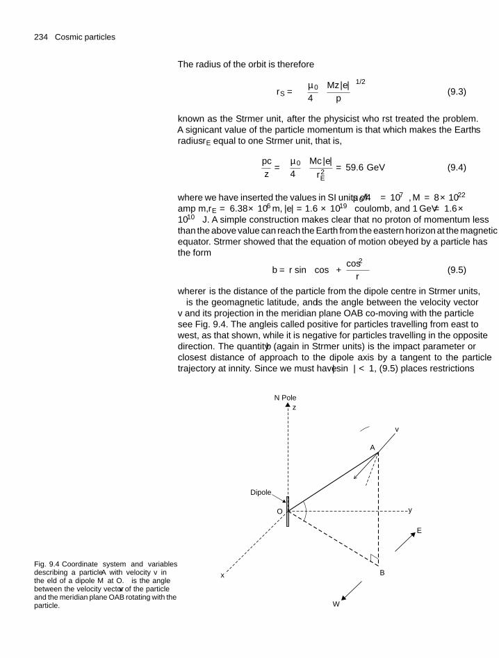
234 Cosmic particles
The radius of the orbit is therefore
rS =[(μ0
4π
) Mz |e|p
]1/2
(9.3)
known as the Stφrmer unit, after the physicist who first treated the problem.A significant value of the particle momentum is that which makes the Earth’sradius rE equal to one Stφrmer unit, that is,
pc
z=(μ0
4π
) Mc |e|r2
E
= 59.6 GeV (9.4)
where we have inserted the values in SI units of μ0/4π = 10−7, M = 8 × 10²²
amp m, rE = 6.38 × 10⁶ m, |e| = 1.6 × 10⁻¹⁹ coulomb, and 1 GeV = 1.6 ×10⁻¹⁰ J. A simple construction makes clear that no proton of momentum lessthan the above value can reach the Earth from the eastern horizon at the magneticequator. Stφrmer showed that the equation of motion obeyed by a particle hasthe form
b = r sin θ cos λ + cos2 λ
r(9.5)
where r is the distance of the particle from the dipole centre in Stφrmer units,λ is the geomagnetic latitude, and θ is the angle between the velocity vectorv and its projection in the meridian plane OAB co-moving with the particle—see Fig. 9.4. The angle θ is called positive for particles travelling from east towest, as that shown, while it is negative for particles travelling in the oppositedirection. The quantity b (again in Stφrmer units) is the impact parameter orclosest distance of approach to the dipole axis by a tangent to the particletrajectory at infinity. Since we must have | sin θ| < 1, (9.5) places restrictions
Fig. 9.4 Coordinate system and variablesdescribing a particle A with velocity v inthe field of a dipole M at O. θ is the anglebetween the velocity vector v of the particleand the meridian plane OAB rotating with theparticle.
O
Dipole
N Pole
�
z
v
A
y
E
B
W
x
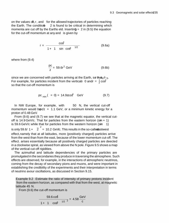
9.3 Geomagnetic and solar effects 235
on the values of b, r, and λ for the ‘allowed’ trajectories of particles reachingthe Earth. The condition b ≤ 2 is found to be critical in determining whichmomenta are cut off by the Earth’s field. Inserting b = 2 in (9.5) the equationfor the cut-off momentum at any λ and θ is given by
r = cos2 λ[1 + (1 − sin θ cos3 λ
)1/2] (9.6a)
where from (9.4)
pc
z= 59.6 r2 GeV (9.6b)
since we are concerned with particles arriving at the Earth, so that r = rE/rS.For example, for particles incident from the vertical, θ = 0 and r = 1
2 cos2 λ
so that the cut-off momentum is
(pc)
min (θ = 0) = 14.9z cos4 λ GeV (9.7)
In NW Europe, for example, with λ ∼ 50◦ N, the vertical cut-offmomentum would be pc/z = 1.1 GeV, or a minimum kinetic energy for aproton of 0.48 GeV.
From (9.6) and (9.7) we see that at the magnetic equator, the vertical cut-off is 14.9 GeV/c. That for particles from the eastern horizon (sin θ = +1)is 59.6 GeV/c while that for particles from the western horizon (sin θ = −1)
is only 59.6/(
1 + √2)2 = 10.2 GeV/c. This results in the so-called east–west
effect, namely that at all latitudes, more (positively charged) particles arrivefrom the west than from the east, because of the lower momentum cut-off. Theeffect. arises essentially because all positively charged particles are deflectedin a clockwise spiral, as viewed from above the N pole. Figure 9.5 shows a mapof the vertical cut-off rigidities.
The azimuthal and latitude dependencies of the primary particles arepromulgated in the secondaries they produce in traversing the atmosphere. Sucheffects are observed, for example, in the interactions of atmospheric neutrinos,coming from the decay of secondary pions and muons, and were important inestablishing the credibility of the experiments and their interpretation in termsof neutrino flavour oscillations, as discussed in Section 9.15.
Example 9.2 Estimate the ratio of intensity of primary protons incidentfrom the eastern horizon, as compared with that from the west, at magneticlatitude 45◦ N.
From (9.6) the cut-off momentum is
59.6 cos4 λ[1 + (1 − cos3 λ
)1/2]2 = 4.58
GeV
c
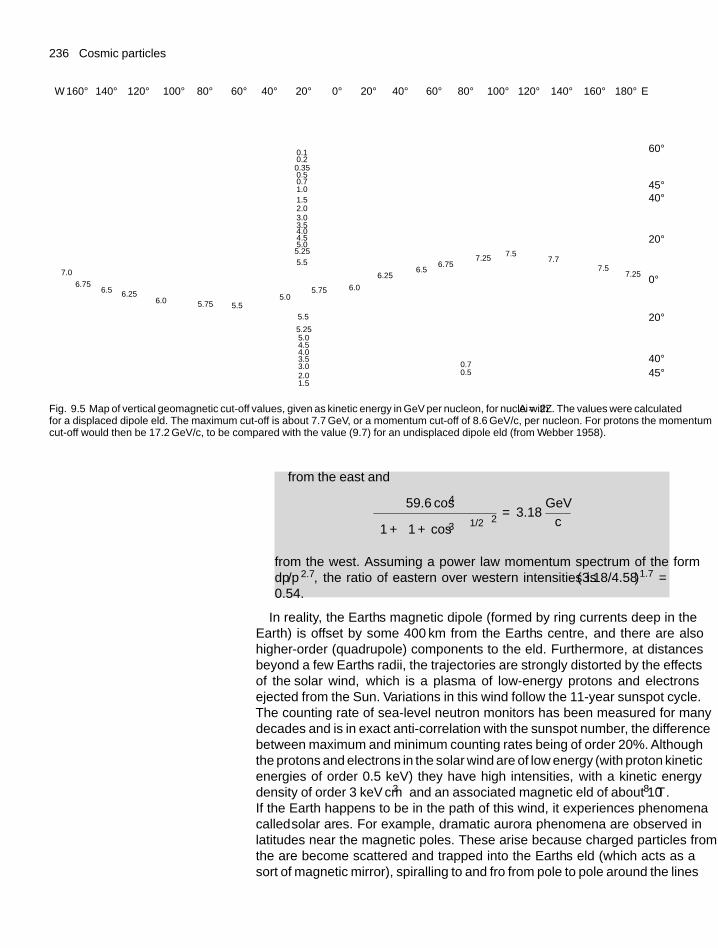
236 Cosmic particles
W 160° 140° 120° 120° 140° 160° 180° E100° 100°80° 80°60° 60°40° 40°20° 20°0°
60°
45°40°
20°
0°
20°
40°45°
7.0
6.0 5.755.0
5.75
0.70.5
6.25
7.25 7.5
7.57.25
7.76.75
6.5
5.5
6.256.56.75
1.52.03.03.54.04.55.0
5.25
5.5
5.255.04.54.03.53.02.01.51.00.70.5
0.350.20.1
6.0
5.5
Fig. 9.5 Map of vertical geomagnetic cut-off values, given as kinetic energy in GeV per nucleon, for nuclei with A = 2Z . The values were calculatedfor a displaced dipole field. The maximum cut-off is about 7.7 GeV, or a momentum cut-off of 8.6 GeV/c, per nucleon. For protons the momentumcut-off would then be 17.2 GeV/c, to be compared with the value (9.7) for an undisplaced dipole field (from Webber 1958).
from the east and
59.6 cos4 λ[1 + (1 + cos3 λ
)1/2]2 = 3.18
GeV
c
from the west. Assuming a power law momentum spectrum of the formdp/p2.7, the ratio of eastern over western intensities is (3.18/4.58)1.7 =0.54.
In reality, the Earth’s magnetic dipole (formed by ring currents deep in theEarth) is offset by some 400 km from the Earth’s centre, and there are alsohigher-order (quadrupole) components to the field. Furthermore, at distancesbeyond a few Earth’s radii, the trajectories are strongly distorted by the effectsof the solar wind, which is a plasma of low-energy protons and electronsejected from the Sun. Variations in this wind follow the 11-year sunspot cycle.The counting rate of sea-level neutron monitors has been measured for manydecades and is in exact anti-correlation with the sunspot number, the differencebetween maximum and minimum counting rates being of order 20%. Althoughthe protons and electrons in the solar wind are of low energy (with proton kineticenergies of order 0.5 keV) they have high intensities, with a kinetic energydensity of order 3 keV cm−3 and an associated magnetic field of about 10−8T .If the Earth happens to be in the path of this wind, it experiences phenomenacalled solar flares. For example, dramatic aurora phenomena are observed inlatitudes near the magnetic poles. These arise because charged particles fromthe flare become scattered and trapped into the Earth’s field (which acts as asort of magnetic mirror), spiralling to and fro from pole to pole around the lines
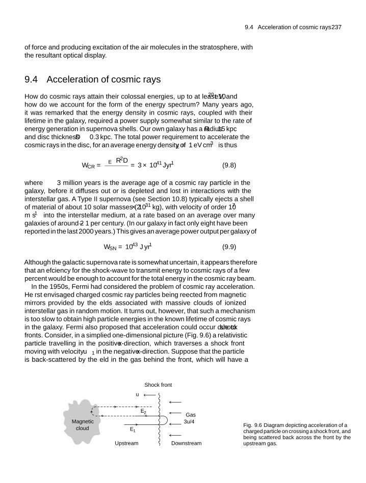
9.4 Acceleration of cosmic rays 237
of force and producing excitation of the air molecules in the stratosphere, withthe resultant optical display.
9.4 Acceleration of cosmic rays
How do cosmic rays attain their colossal energies, up to at least 1020 eV, andhow do we account for the form of the energy spectrum? Many years ago,it was remarked that the energy density in cosmic rays, coupled with theirlifetime in the galaxy, required a power supply somewhat similar to the rate ofenergy generation in supernova shells. Our own galaxy has a radius R ∼ 15 kpcand disc thickness D ∼ 0.3 kpc. The total power requirement to accelerate thecosmic rays in the disc, for an average energy density of ρE = 1 eV cm−3 is thus
WCR = ρEπR2D
τ= 3 × 1041 Jyr−1 (9.8)
where τ ∼ 3 million years is the average age of a cosmic ray particle in thegalaxy, before it diffuses out or is depleted and lost in interactions with theinterstellar gas. A Type II supernova (see Section 10.8) typically ejects a shellof material of about 10 solar masses (2 × 1031 kg), with velocity of order 107
m s−1 into the interstellar medium, at a rate based on an average over manygalaxies of around 2±1 per century. (In our galaxy in fact only eight have beenreported in the last 2000 years.) This gives an average power output per galaxy of
WSN = 1043 J yr−1 (9.9)
Although the galactic supernova rate is somewhat uncertain, it appears thereforethat an efficiency for the shock-wave to transmit energy to cosmic rays of a fewpercent would be enough to account for the total energy in the cosmic ray beam.
In the 1950s, Fermi had considered the problem of cosmic ray acceleration.He first envisaged charged cosmic ray particles being reflected from ‘magneticmirrors’ provided by the fields associated with massive clouds of ionizedinterstellar gas in random motion. It turns out, however, that such a mechanismis too slow to obtain high particle energies in the known lifetime of cosmic raysin the galaxy. Fermi also proposed that acceleration could occur due to shockfronts. Consider, in a simplified one-dimensional picture (Fig. 9.6) a relativisticparticle travelling in the positive x-direction, which traverses a shock frontmoving with velocity −u1 in the negative x-direction. Suppose that the particleis back-scattered by the field in the gas behind the front, which will have a
Magneticcloud
Shock front
Upstream Downstream
E2
E1
–u
Gas–3u/4
Fig. 9.6 Diagram depicting acceleration of acharged particle on crossing a shock front, andbeing scattered back across the front by theupstream gas.
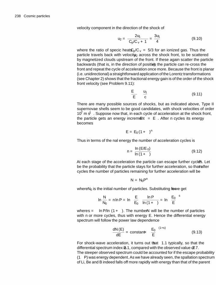
238 Cosmic particles
velocity component in the direction of the shock of
u2 = 2u1(Cp/Cv + 1
) = 3u1
4(9.10)
where the ratio of specific heats Cp/Cv = 5/3 for an ionized gas. Thus theparticle travels back with velocity u2 across the shock front, to be scatteredby magnetized clouds upstream of the front. If these again scatter the particlebackwards (that is, in the direction of positive x), the particle can re-cross thefront and repeat the cycle of acceleration once more. Because the front is planar(i.e. unidirectional) a straightforward application of the Lorentz transformations(see Chapter 2) shows that the fractional energy gain is of the order of the shockfront velocity (see Problem 9.11):
�E
E∼ u1
c(9.11)
There are many possible sources of shocks, but as indicated above, Type IIsupernovae shells seem to be good candidates, with shock velocities of order107 m s−1. Suppose now that, in each cycle of acceleration at the shock front,the particle gets an energy increment �E = αE. After n cycles its energybecomes
E = E0 (1 + α)n
Thus in terms of the final energy the number of acceleration cycles is
n = ln (E/E0)
ln (1 + α)(9.12)
At each stage of the acceleration the particle can escape further cycles. Let Pbe the probability that the particle stays for further acceleration, so that after ncycles the number of particles remaining for further acceleration will be
N = N0Pn
where N0 is the initial number of particles. Substituting for n we get
lnN
N0= n ln P = ln
(E
E0
)ln P
ln (1 + α)= ln
(E0
E
)s
where s = −ln P/ln (1 + α). The number N will be the number of particleswith n or more cycles, thus with energy ≥ E. Hence the differential energyspectrum will follow the power law dependence
dN (E)
dE= constant ×
(E0
E
)(1+s)
(9.13)
For shock-wave acceleration, it turns out that s ∼ 1.1 typically, so that thedifferential spectrum index is −2.1, compared with the observed value of −2.7.The steeper observed spectrum could be accounted for if the escape probability(1−P) was energy dependent. As we have already seen, the spallation spectrumof Li, Be and B indeed falls off more rapidly with energy than that of the parent
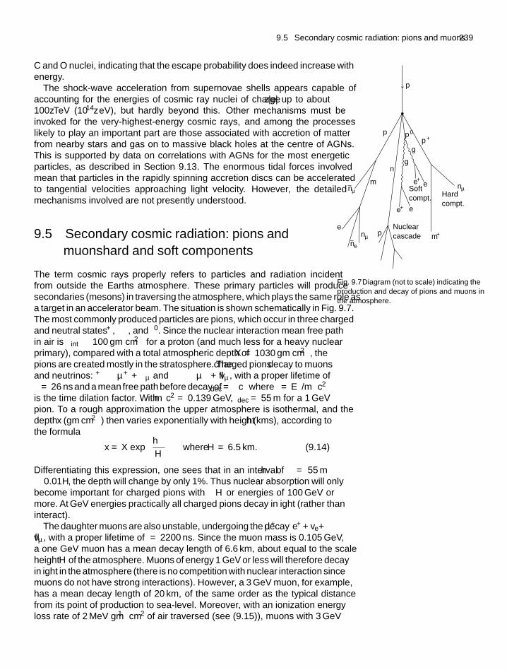
9.5 Secondary cosmic radiation: pions and muons 239
C and O nuclei, indicating that the escape probability does indeed increase withenergy.
The shock-wave acceleration from supernovae shells appears capable ofaccounting for the energies of cosmic ray nuclei of charge z|e| up to about100z TeV (1014z eV), but hardly beyond this. Other mechanisms must beinvoked for the very-highest-energy cosmic rays, and among the processeslikely to play an important part are those associated with accretion of matterfrom nearby stars and gas on to massive black holes at the centre of AGNs.This is supported by data on correlations with AGNs for the most energeticparticles, as described in Section 9.13. The enormous tidal forces involvedmean that particles in the rapidly spinning accretion discs can be acceleratedto tangential velocities approaching light velocity. However, the detailedmechanisms involved are not presently understood.
9.5 Secondary cosmic radiation: pions andmuons—hard and soft components
g
g
p
p+
e+
e+
m+
p0p–
e–
e–
e–
p
n
Softcompt. Hard
compt.
Nuclearcascade
nμ
nμ
nμ
ne
m–
Fig. 9.7 Diagram (not to scale) indicating theproduction and decay of pions and muons inthe atmosphere.
The term ‘cosmic rays’ properly refers to particles and radiation incidentfrom outside the Earth’s atmosphere. These primary particles will producesecondaries (mesons) in traversing the atmosphere, which plays the same role asa target in an accelerator beam. The situation is shown schematically in Fig. 9.7.The most commonly produced particles are pions, which occur in three chargedand neutral states π+, π−, and π0. Since the nuclear interaction mean free pathin air is λint ∼ 100 gm cm−2 for a proton (and much less for a heavy nuclearprimary), compared with a total atmospheric depth of X = 1030 gm cm−2, thepions are created mostly in the stratosphere. The charged pions decay to muonsand neutrinos: π+ → μ+ + νμ and π− → μ− + vμ, with a proper lifetime ofτ = 26 ns and a mean free path before decay of λdec = γcτ where γ = Eπ/mπc2
is the time dilation factor. With mπc2 = 0.139 GeV, λdec = 55 m for a 1 GeVpion. To a rough approximation the upper atmosphere is isothermal, and thedepth x (gm cm−2) then varies exponentially with height h (kms), according tothe formula
x = X exp
(−h
H
)where H = 6.5 km. (9.14)
Differentiating this expression, one sees that in an interval �h of λ = 55 m∼ 0.01H , the depth will change by only 1%. Thus nuclear absorption will onlybecome important for charged pions with λ ∼ H or energies of 100 GeV ormore. At GeV energies practically all charged pions decay in flight (rather thaninteract).
The daughter muons are also unstable, undergoing the decay μ+ → e++ve+vμ, with a proper lifetime of τ = 2200 ns. Since the muon mass is 0.105 GeV,a one GeV muon has a mean decay length of 6.6 km, about equal to the scaleheight H of the atmosphere. Muons of energy 1 GeV or less will therefore decayin flight in the atmosphere (there is no competition with nuclear interaction sincemuons do not have strong interactions). However, a 3 GeV muon, for example,has a mean decay length of 20 km, of the same order as the typical distancefrom its point of production to sea-level. Moreover, with an ionization energyloss rate of 2 MeV gm−1 cm2 of air traversed (see (9.15)), muons with 3 GeV
240 Cosmic particles
or more energy can get through the entire atmosphere without being brought torest or decaying. Still higher-energy muons can reach deep underground, andfor this reason they are said to constitute the hard component of the cosmicradiation. The remaining products of charged pion and muon production, theneutrinos, are discussed in Section 9.15.
The neutral pions undergo electromagnetic decay, π0 → 2γ , with anextremely short lifetime of 8 × 10⁻¹⁷ s. The photons from the decay developelectron–photon cascades, as described below, mostly in the high atmosphere,since the absorption length of these cascades is short compared with the totalatmospheric depth. The electrons and photons of these cascades constitute theeasily absorbed soft component of the cosmic radiation.
Among the products of the nuclear interactions of primary cosmic rays in theatmosphere are radioactive isotopes, of which an important one is 14C formed,for example, by neutron capture in nitrogen: n+14N →14 C+1H.The 14C atomsproduced in this way combine to form CO2 molecules and thus participate,like the more common, stable 12C atoms, in the circulation of this gas in theatmosphere, through rainfall into the oceans, and in absorption in organic matter.Since carbon-14 has a mean lifetime of 5600 years, its abundance relative tocarbon-12 in organic matter can be used to date the sample. This of courseassumes that the carbon-14 production rate by cosmic rays has been constantwith time. In fact, comparison of the age from the isotope ratio with that fromancient tree ring counts shows that the cosmic ray intensity did vary in thepast and was some 20% larger 5000 years ago. This variation was presumablydue to long-term fluctuations in the value of the Earth’s magnetic field which,associated with continental drift, is known from rock samples to have changedits sign and magnitude many times over geological time.
9.6 Passage of charged particles and radiationthrough matter
As a preliminary to discussing the subjects of γ-ray sources and extensive airshowers, we include here a summary of the interactions of charged particlesand radiation as they traverse matter, in solid materials and in the atmosphere.
9.6.1 Ionization energy losses
Charged particles lose energy as a result of collisions with atomic electrons,leading to ionization of the atoms. The rate of ionization energy loss is givenby the Bethe–Bloch formula(
dE
dx
)ion
=(
4πN0z2e4
mv2
)(Z
A
){ln
[2mv2γ2
I
]− β2
}(9.15)
where m is the electron mass and v and ze are the velocity and charge of theincident particle, β = v/c, γ2 = 1/
(1 − β2
), N0 is Avogadro’s number, Z and
A are the atomic and mass numbers of the atoms of the medium, and x is the pathlength in the medium, usually measured in g cm−2. The quantity I is the meanionization potential of the medium, averaged over all electrons in the atom, andis approximately I ≈ 10 Z eV. Notice that dE/dx is a function of velocity v and
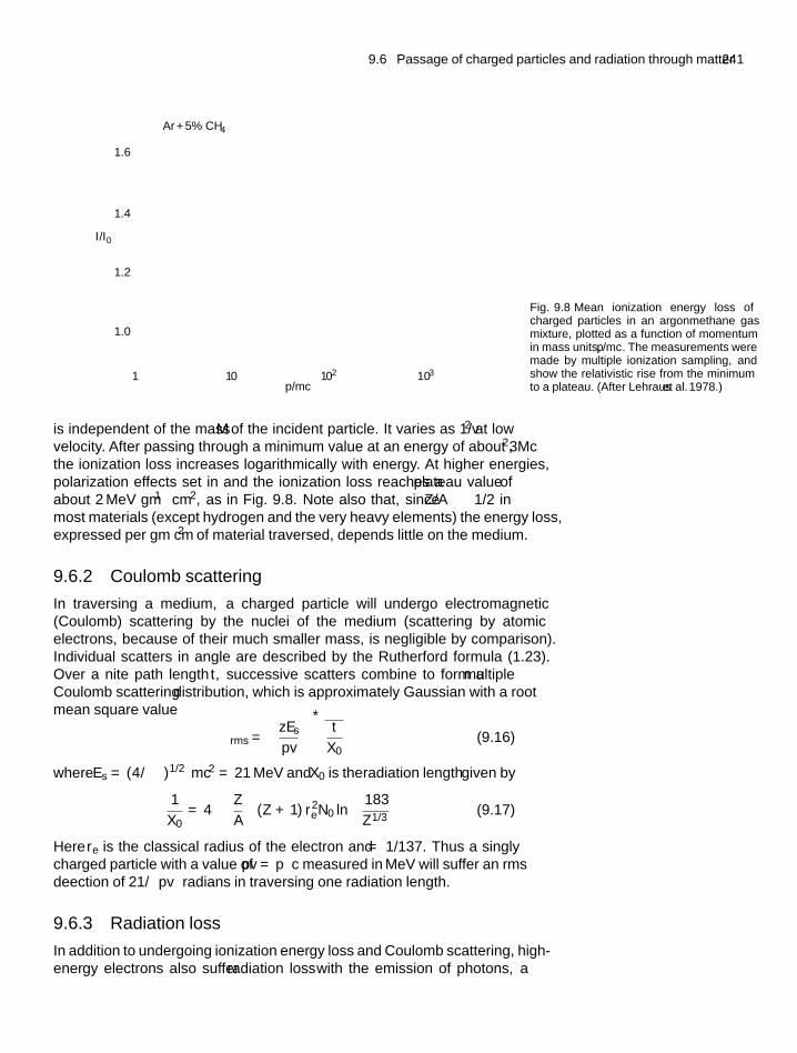
9.6 Passage of charged particles and radiation through matter 241
1.6
Ar + 5% CH4
1.4
1.2
1.0
1 10 102
p/mc103
I/I0
Fig. 9.8 Mean ionization energy loss ofcharged particles in an argon–methane gasmixture, plotted as a function of momentumin mass units, p/mc. The measurements weremade by multiple ionization sampling, andshow the relativistic rise from the minimumto a plateau. (After Lehraus et al. 1978.)
is independent of the mass M of the incident particle. It varies as 1/v2 at lowvelocity. After passing through a minimum value at an energy of about 3Mc2,the ionization loss increases logarithmically with energy. At higher energies,polarization effects set in and the ionization loss reaches a plateau value ofabout 2 MeV gm−1 cm2, as in Fig. 9.8. Note also that, since Z/A ∼ 1/2 inmost materials (except hydrogen and the very heavy elements) the energy loss,expressed per gm cm−2 of material traversed, depends little on the medium.
9.6.2 Coulomb scattering
In traversing a medium, a charged particle will undergo electromagnetic(Coulomb) scattering by the nuclei of the medium (scattering by atomicelectrons, because of their much smaller mass, is negligible by comparison).Individual scatters in angle are described by the Rutherford formula (1.23).Over a finite path length t, successive scatters combine to form a multipleCoulomb scattering distribution, which is approximately Gaussian with a rootmean square value
ϕrms =(
zEs
pv
)√t
X0(9.16)
where Es = (4π/α)1/2 mc2 = 21 MeV and X0 is the radiation length given by
1
X0= 4α
(Z
A
)(Z + 1) r2
e N0 ln
(183
Z1/3
)(9.17)
Here re is the classical radius of the electron and α = 1/137. Thus a singlycharged particle with a value of pv = pβc measured in MeV will suffer an rmsdeflection of 21/
(pv)
radians in traversing one radiation length.
9.6.3 Radiation loss
In addition to undergoing ionization energy loss and Coulomb scattering, high-energy electrons also suffer radiation loss with the emission of photons, a
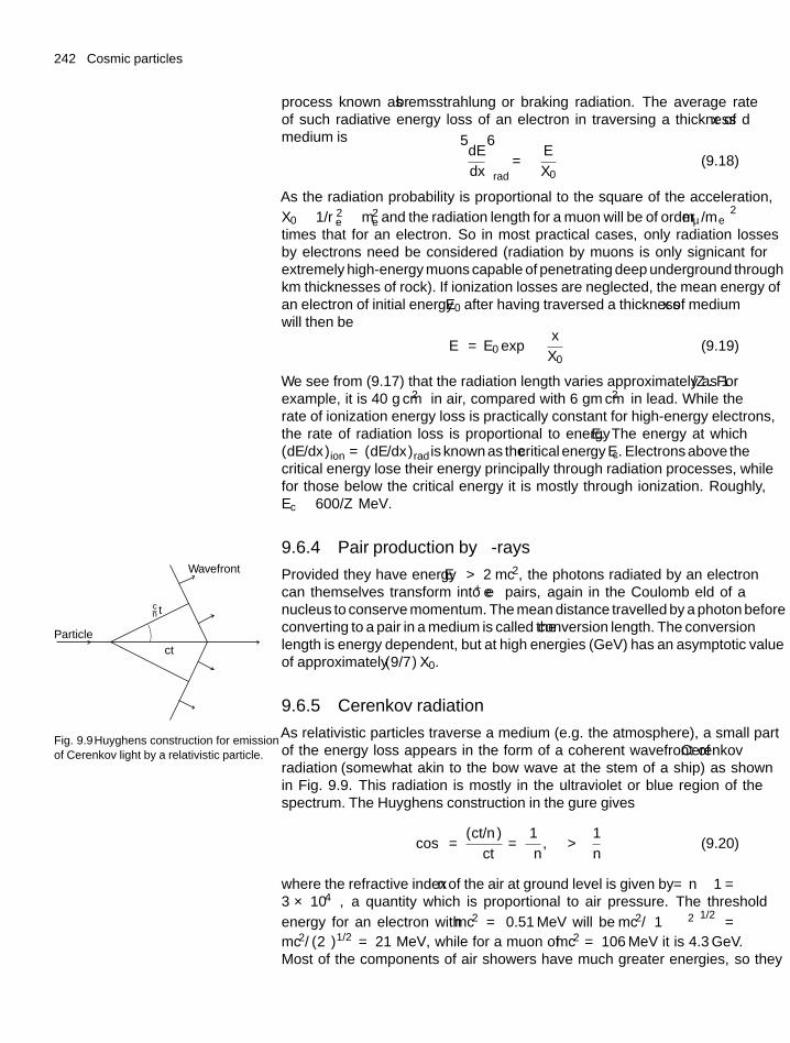
242 Cosmic particles
process known as ‘bremsstrahlung’ or braking radiation. The average rateof such radiative energy loss of an electron in traversing a thickness dx ofmedium is ⟨
dE
dx
⟩rad
= − E
X0(9.18)
As the radiation probability is proportional to the square of the acceleration,X0 ∝ 1/r2
e ∝ m2e and the radiation length for a muon will be of order
(mμ/me
)2times that for an electron. So in most practical cases, only radiation lossesby electrons need be considered (radiation by muons is only significant forextremely high-energy muons capable of penetrating deep underground throughkm thicknesses of rock). If ionization losses are neglected, the mean energy ofan electron of initial energy E0 after having traversed a thickness x of mediumwill then be
〈E〉 = E0 exp
(− x
X0
)(9.19)
We see from (9.17) that the radiation length varies approximately as 1/Z . Forexample, it is 40 g cm−2 in air, compared with 6 gm cm−2 in lead. While therate of ionization energy loss is practically constant for high-energy electrons,the rate of radiation loss is proportional to energy E. The energy at which(dE/dx)ion = (dE/dx)rad is known as the critical energy Ec. Electrons above thecritical energy lose their energy principally through radiation processes, whilefor those below the critical energy it is mostly through ionization. Roughly,Ec ∼ 600/Z MeV.
9.6.4 Pair production by γ -rays
Provided they have energy Eγ > 2 mc2, the photons radiated by an electroncan themselves transform into e+e− pairs, again in the Coulomb field of anucleus to conserve momentum. The mean distance travelled by a photon beforeconverting to a pair in a medium is called the conversion length. The conversionlength is energy dependent, but at high energies (GeV) has an asymptotic valueof approximately (9/7) X0.
9.6.5 Cerenkov radiation
Particle
Wavefront
tcn
�ct�
Fig. 9.9 Huyghens construction for emissionof Cerenkov light by a relativistic particle.
As relativistic particles traverse a medium (e.g. the atmosphere), a small partof the energy loss appears in the form of a coherent wavefront of Cerenkovradiation (somewhat akin to the bow wave at the stem of a ship) as shownin Fig. 9.9. This radiation is mostly in the ultraviolet or blue region of thespectrum. The Huyghens construction in the figure gives
cos θ = (ct/n)
βct= 1
βn, β >
1
n(9.20)
where the refractive index n of the air at ground level is given by ε = n − 1 =3 × 10⁻⁴, a quantity which is proportional to air pressure. The threshold
energy for an electron with mc2 = 0.51 MeV will be mc2/(1 − β2
)1/2 =mc2/(2ε)1/2 = 21 MeV, while for a muon of mc2 = 106 MeV it is 4.3 GeV.Most of the components of air showers have much greater energies, so they
9.7 Development of an electromagnetic cascade 243
will produce abundant Cerenkov light. Typically, a relativistic particle abovethreshold generates about 10,000 photons per km of path near ground level (andless at high altitudes where the pressure is lower). This light can be detectedby means of large spherical mirror arrays which direct it on to photomultipliersplaced at the focus (see Fig. 9.11).
9.6.6 Atmospheric fluorescence
Charged particles traversing the atmosphere not only ionize, but also excitethe atoms. Some of this appears in the form of fluorescence from nitrogenmolecules, with typically 5000 photons per km of track length, again in the bluewavelength region (300–450 nm).This fluorescent light is emitted isotropically.On the other hand, Cerenkov light from atmospheric traversal by extremerelativistic particles is emitted in a narrow cone of angle θ ∼ (2ε)1/2(= 1.4◦ atground level, although Coulomb scattering of the electrons will considerablybroaden this). This distinction is important from the point of view of showerdetection, as described below.
9.7 Development of an electromagnetic cascade
We now discuss the longitudinal development of an electromagnetic showerin very simplified terms. Consider an electron of initial energy E0 traversinga medium, neglecting ionization losses. In the first radiation length, supposethe electron radiates one photon, of energy E0/2. In the next radiation length,suppose the photon converts to an electron–positron pair, each with energyE0/4, and that the original electron radiates a further photon, also of energyE0/4. Thus, after two radiation lengths, we have one photon, two electrons,and one positron, each of them with the energy E0/4. Proceeding in this way,it follows that after t radiation lengths, we shall have electrons, positrons, andphotons in approximately equal numbers, each with energy E (t) = E0/2t .We assume that this cascade multiplication process continues until the particleenergy falls to E = Ec, the critical energy, when we suppose that ionizationloss suddenly becomes dominant and that no further radiation or pair conversionprocesses are possible. Thus the cascade reaches a maximum and then ceasesabruptly. The main features of this simple model are the following:
• The shower maximum is at a depth t = t (max) = ln (E0/Ec)/ln 2, thatis, it increases logarithmically with primary energy E0.
• The number of particles at shower maximum is N (max) = 2t(max) =E0/Ec, that is, proportional to the primary energy.
• The number of shower particles above energy E is equal to the numbercreated at depths less than t(E), that is,
N (> E) =∫
2tdt =∫
exp (t ln 2) dt = (E0/E)
ln 2.
so that the differential energy spectrum of the particles is
dN
dE∝ dE
E2.
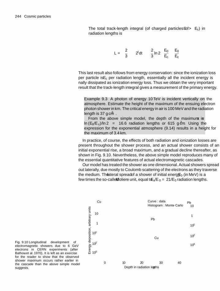
244 Cosmic particles
• The total track-length integral (of charged particles of E > Ec) inradiation lengths is
L =(
2
3
)∫2tdt ∼
(2
3ln 2
)E0
Ec∼ E0
Ec
This last result also follows from energy conservation: since the ionization lossper particle is Ec per radiation length, essentially all the incident energy isfinally dissipated as ionization energy loss. Thus we obtain the very importantresult that the track-length integral gives a measurement of the primary energy.
Example 9.3 A photon of energy 10 TeV is incident vertically on theatmosphere. Estimate the height of the maximum of the ensuing electron–photon shower in km. The critical energy in air is 100 MeV and the radiationlength is 37 g cm−2.
From the above simple model, the depth of the maximum is x =ln (E0/Ec)/ln 2 = 16.6 radiation lengths or 615 g cm−2. Using theexpression for the exponential atmosphere (9.14) results in a height forthe maximum of 3.4 km.
In practice, of course, the effects of both radiation and ionization losses arepresent throughout the shower process, and an actual shower consists of aninitial exponential rise, a broad maximum, and a gradual decline thereafter, asshown in Fig. 9.10. Nevertheless, the above simple model reproduces many ofthe essential quantitative features of actual electromagnetic cascades.
Our model has treated the shower as one dimensional. Actual showers spreadout laterally, due mostly to Coulomb scattering of the electrons as they traversethe medium. The lateral spread of a shower of initial energy E0 (in MeV) is afew times the so-called Moliere unit, equal to Es/E0 = 21/E0 radiation lengths.
Fig. 9.10 Longitudinal development ofelectromagnetic showers due to 6 GeVelectrons in CERN experiments (afterBathow et al. 1970). It is left as an exercisefor the reader to show that the observedshower maximum occurs rather earlier inthe cascade than the above simple modelsuggests.
Cu
Cu
Pb
Pb
Curve : dataHistogram : Monte Carlo
10
0 10 20Depth in radiation lengths
Ene
rgy
depo
sitio
n, a
rbitr
ary
units
30 40
1
10–1
10–2
10–3
10
1
10–1
10–2
10–3
→
9.9 Detection of extensive air showers 245
9.8 Extensive air showers: nucleon- andphoton-induced showers
If the primary particle is a high-energy proton or heavier nucleus rather than anelectron or photon, a nuclear cascade will develop through the atmosphere. Thelongitudinal scale is the nuclear interaction length in air, λint ∼ 100 gm cm−2.The proton (or heavier nucleus) generates mesons in these interactions, andthey can in turn generate further particles in subsequent collisions. While,in the electron–photon shower, the electrons lose the bulk of their energiesin a radiation length, the nucleons can in general penetrate through severalinteraction lengths, losing only a fraction of their energy—typically 25%—in each encounter, to struck nucleons as well as mesons. In air, the nuclearinteraction length is some 2.5 times the radiation length X0 ∼ 40 gm cm−2.Thus cascades initiated by nucleons are very much more penetrating thanpurely electromagnetic cascades initiated by photons, and this difference inthe shower profile through the atmosphere has been exploited to differentiatebetween nucleon- and photon-induced cascades.
Another difference is that the lateral spread of nuclear showers is determinedmostly by the transverse momentum of the secondaries in nuclear interactions,typically 0.3 GeV/c, and is much larger than for an electromagnetic shower ofthe same primary energy. Such extensive air showers will contain a high-energycore, predominantly of nucleons, with a more widely spread electron–photoncomponent which is continually fed by fresh neutral pion production and decay,π0 → 2γ , and fresh electromagnetic cascades. As mentioned in Section 9.6,the pion decay probability at high energy falls off as 100/Eπ(GeV), so thatapart from a small amount of energy in the form of neutrinos and muons frompion decay, the great bulk of the energy as well as the overwhelming majority ofthe particles in a proton-initiated extensive air shower will end up in electron–photon cascades. So the track-length integral will again give a measure of theprimary energy of the shower. However, the interpretation of the actual signalsrecorded by either ground arrays or air Cerenkov/fluorescence detectors doesdepend to some extent on the modelling used to simulate the nucleon cascade,and it is noteworthy that the inferred fluxes from the AGASA, HiRes, andAUGER arrays differ typically by a factor of up to 2.
9.9 Detection of extensive air showers
The detection of extensive air showers has been accomplished by a varietyof techniques. The oldest technique, pioneered by Auger more than 75 yearsago, uses an extended array of ground detectors in coincidence. These grounddetection detectors sample the charged particles in the shower, usually by meansof tanks containing liquid scintillator or water Cerenkov counters. Such showersonly become detectable at sea-level for primary energies E0 > 1000 TeV(1015eV), when the maximum occurs near the ground. At mountain altitudes,the threshold is typically 100 TeV. The particles in such showers all have v ∼ c,so that the shower front is quite well defined, and the direction of the primaryparticle can be measured rather accurately by timing the different parts of theshower front as it crosses the array.
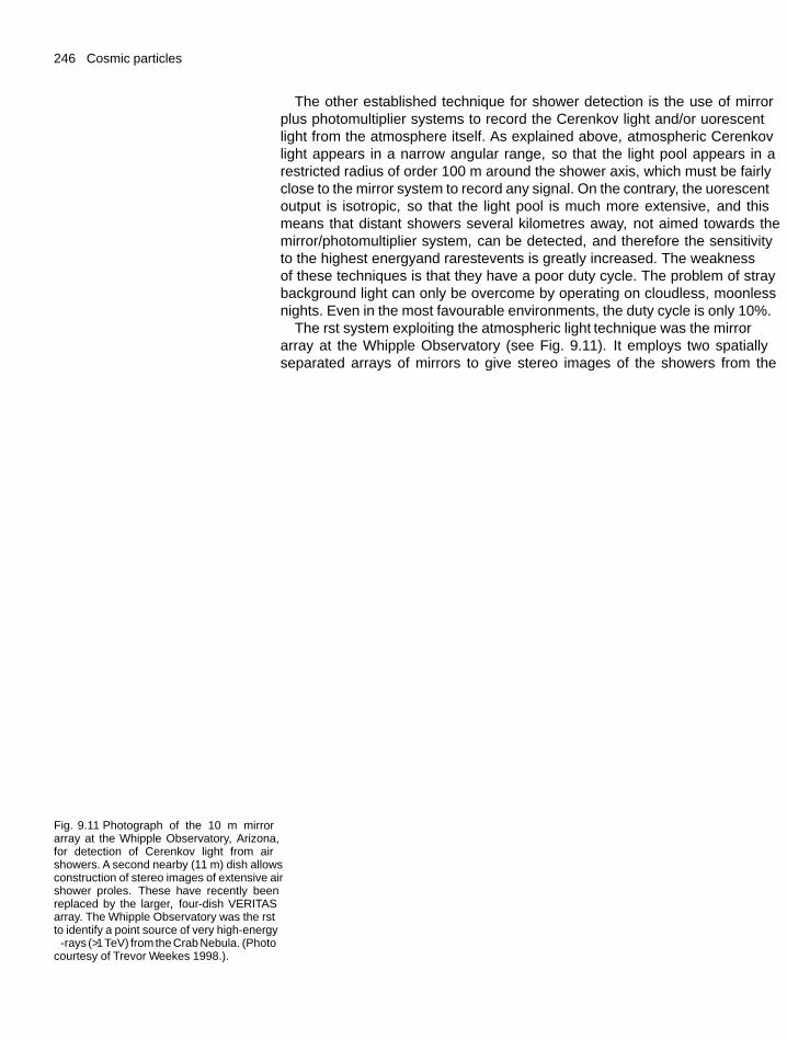
246 Cosmic particles
The other established technique for shower detection is the use of mirrorplus photomultiplier systems to record the Cerenkov light and/or fluorescentlight from the atmosphere itself. As explained above, atmospheric Cerenkovlight appears in a narrow angular range, so that the light pool appears in arestricted radius of order 100 m around the shower axis, which must be fairlyclose to the mirror system to record any signal. On the contrary, the fluorescentoutput is isotropic, so that the light pool is much more extensive, and thismeans that distant showers several kilometres away, not aimed towards themirror/photomultiplier system, can be detected, and therefore the sensitivityto the highest energy—and rarest—events is greatly increased. The weaknessof these techniques is that they have a poor duty cycle. The problem of straybackground light can only be overcome by operating on cloudless, moonlessnights. Even in the most favourable environments, the duty cycle is only 10%.
The first system exploiting the ‘atmospheric light’ technique was the mirrorarray at the Whipple Observatory (see Fig. 9.11). It employs two spatiallyseparated arrays of mirrors to give stereo images of the showers from the
Fig. 9.11 Photograph of the 10 m mirrorarray at the Whipple Observatory, Arizona,for detection of Cerenkov light from airshowers. A second nearby (11 m) dish allowsconstruction of stereo images of extensive airshower profiles. These have recently beenreplaced by the larger, four-dish VERITASarray. The Whipple Observatory was the firstto identify a point source of very high-energyγ-rays (>1TeV) from the Crab Nebula. (Photocourtesy of Trevor Weekes 1998.).
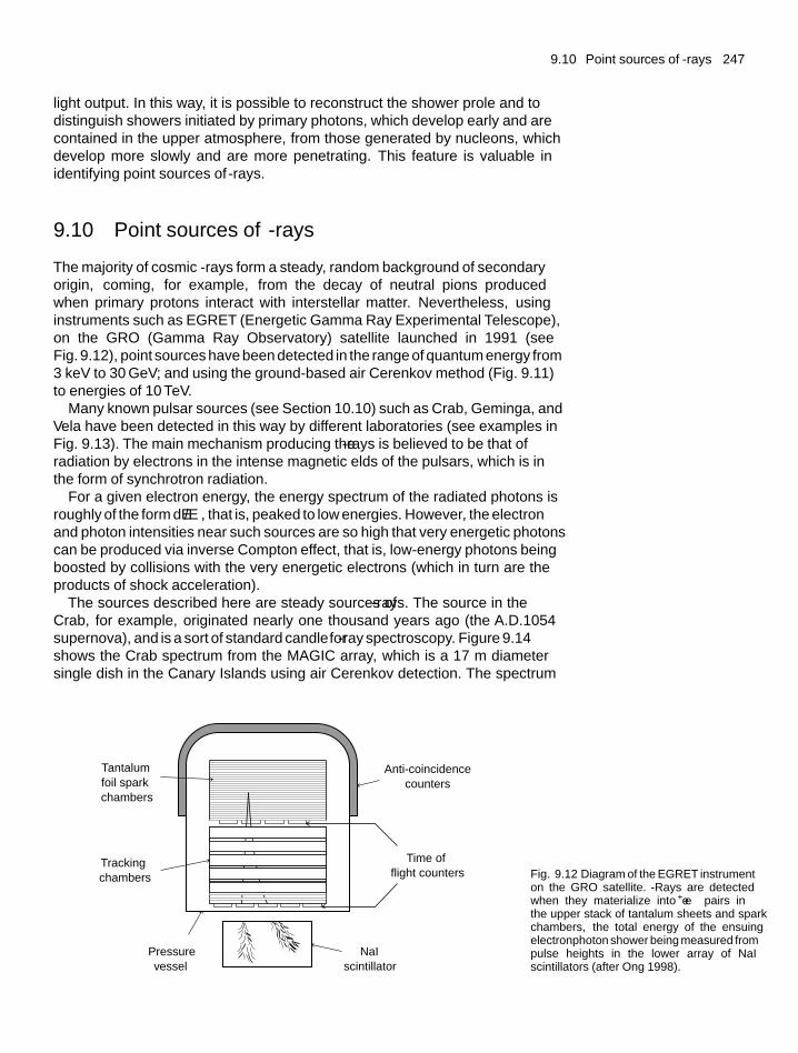
9.10 Point sources of γ-rays 247
light output. In this way, it is possible to reconstruct the shower profile and todistinguish showers initiated by primary photons, which develop early and arecontained in the upper atmosphere, from those generated by nucleons, whichdevelop more slowly and are more penetrating. This feature is valuable inidentifying point sources of γ-rays.
9.10 Point sources of γ -rays
The majority of cosmic γ-rays form a steady, random background of secondaryorigin, coming, for example, from the decay of neutral pions producedwhen primary protons interact with interstellar matter. Nevertheless, usinginstruments such as EGRET (Energetic Gamma Ray Experimental Telescope),on the GRO (Gamma Ray Observatory) satellite launched in 1991 (seeFig. 9.12), point sources have been detected in the range of quantum energy from3 keV to 30 GeV; and using the ground-based air Cerenkov method (Fig. 9.11)to energies of 10 TeV.
Many known pulsar sources (see Section 10.10) such as Crab, Geminga, andVela have been detected in this way by different laboratories (see examples inFig. 9.13). The main mechanism producing the γ-rays is believed to be that ofradiation by electrons in the intense magnetic fields of the pulsars, which is inthe form of synchrotron radiation.
For a given electron energy, the energy spectrum of the radiated photons isroughly of the form dE/E, that is, peaked to low energies. However, the electronand photon intensities near such sources are so high that very energetic photonscan be produced via inverse Compton effect, that is, low-energy photons beingboosted by collisions with the very energetic electrons (which in turn are theproducts of shock acceleration).
The sources described here are steady sources of γ-rays. The source in theCrab, for example, originated nearly one thousand years ago (the A.D.1054supernova), and is a sort of ‘standard candle’for γ-ray spectroscopy. Figure 9.14shows the Crab spectrum from the MAGIC array, which is a 17 m diametersingle dish in the Canary Islands using air Cerenkov detection. The spectrum
Time offlight counters
NaIscintillator
Pressurevessel
Trackingchambers
Tantalumfoil sparkchambers
Anti-coincidencecounters
Fig. 9.12 Diagram of the EGRET instrumenton the GRO satellite. γ-Rays are detectedwhen they materialize into e+e− pairs inthe upper stack of tantalum sheets and sparkchambers, the total energy of the ensuingelectron–photon shower being measured frompulse heights in the lower array of NaIscintillators (after Ong 1998).
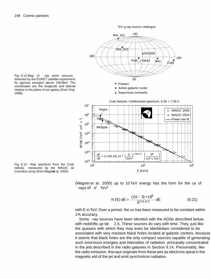
248 Cosmic particles
Fig. 9.13 Map of γ-ray point sourcesdetected by the EGRET satellite experiment,for gamma energies above 100 MeV. Thecoordinates are the longitude and latituderelative to the plane of our galaxy (from Ong1998).
Pulsars
–90
180
+90
TeV g-ray source catalogue
Mrk_421
Mrk_501
PSR_1706–44 Velo Crab
SN1006
–180
Active galactic nuclei
Supernova remnants
Fig. 9.14 γ-Ray spectrum from the Crabnebula, measured by the MAGIC airCerenkov array (from Wagner et al. 2005).
10–7
10–8
Hegra
Whipple10–9
10–10
10–11
102 103
E [GeV]
Crab Nebula · Defferential spectrum, 5.50 + 7.05 h
dF/d
E [
TeV
–1 c
m–2
s–1 ]
104
10–12
10–13
MAGIC 2005
MAGIC 2004Power law fit
dF(1.500.18) 10–3
dEE ph
cm2 s TeVGeV=
–2.580.16
(Wagner et al. 2005) up to 10 TeV energy has the form for the flux ofγ-rays m−2 s−1 TeV−1
N (E) dE = (24 ± 3) · 10−8
E2.6±0.2dE (9.21)
with E in TeV. Over a period, the flux has been measured to be constant within1% accuracy.
Some γ-ray sources have been identified with the AGNs described below,with redshifts up to z ∼ 2.5. These sources do vary with time. They, just likethe quasars –with which they may even be identified—are considered to beassociated with very massive black holes located at galactic centres, becauseit seems that black holes are the only compact sources capable of generatingsuch enormous energies and intensities of radiation, principally concentratedin the ‘jets’ described in the radio galaxies in Section 9.14. Presumably, likethe radio emission, the γ-rays originate from these jets as electrons spiral in themagnetic field of the jet and emit synchrotron radiation.
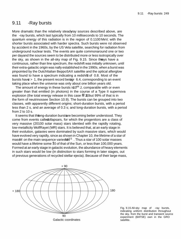
9.11 γ-Ray bursts 249
9.11 γ -Ray bursts
More dramatic than the relatively steady γ-ray sources described above, arethe γ-ray bursts, which last typically from 10 milliseconds to 10 seconds. Thequantum energy of this radiation is in the region of 0.1–100 MeV, with theshorter bursts associated with harder spectra. Such bursts were first observedby accident in the 1960s, by the US Vela satellite, searching for radiation fromunderground nuclear tests. The events are quite common—around one or twoper day—and the sources seem to be distributed more or less isotropically overthe sky, as shown in the all-sky map of Fig. 9.15. Since the γ rays have acontinuous, rather than line spectrum, the redshift was initially unknown, untiltheir extra-galactic origin was finally established in the 1990s, when a burst waspinpointed by the Dutch–Italian BeppoSAX satellite and the optical afterglowwas found to have a spectrum indicating a redshift of z ∼ 0.8. Most of thebursts have z > 1, the present record being z = 6.4, corresponding to an eventtaking place when the universe was only about one billion years old.
The amount of energy in these bursts is ∼ 1044 J, comparable with or evengreater than that emitted (in photons) in the course of a Type II supernovaexplosion (the total energy release in this case is 1046 J, but 99% of that is inthe form of neutrinos—see Section 10.9). The bursts can be grouped into twoclasses, with apparently different origins; short-duration bursts, with a periodless than 2 s, and an average of 0.3 s; and long-duration bursts, with a periodfrom 2 to 10 s.
It seems that the long-duration bursts are becoming better understood. Theycome from events called collapsars, for which the progenitors are a class ofvery massive (20–100 solar mass) stars identified with the rapidly rotating,low-metallicity Wolf–Rayet (W–R) stars. It is believed that, at an early stage intheir evolution, galaxies were dominated by such massive stars, which wouldhave evolved very rapidly, since as shown in Chapter 10, the lifetime of a star ofmass M on the main sequence varies as M −2.5. Thus a star of 100 solar masseswould have a lifetime some 10−5 of that of the Sun, or less than 100,000 years.Formed at an early stage in galactic evolution, the abundance of heavy elementsin such stars would be low (in distinction to stars forming in later stages, outof previous generations of recycled stellar ejecta). Because of their large mass,
+ 90
+ 180 – 180
– 90Galactic coordinates
Fig. 9.15 All-sky map of γ-ray bursts,indicating uniform distribution throughoutthe sky, from the burst and transient sourceexperiment (BATSE) flown in the GROsatellite.
250 Cosmic particles
the W–R stars evolve rapidly, and at the end of silicon burning, the core of suchstars is believed to collapse directly to a black hole—as distinct from stars oflower mass—passing first through the neutron star stage. The blast of γ-raysaccompanies the enormous energy released when the surrounding material inthe accretion disc is sucked into the black hole.
We should note here that, as will be explained in Chapter 10, stars form fromaccumulating interstellar gas falling into orbital motion about the centre of mass,and this so-called protostar evolves through successive stages of thermonuclearburning, with increasing temperature and enormous contraction of the core.Because of contraction and conservation of angular momentum, the core willgenerally be rapidly rotating. As in the case of quasars, because of the torusshape of the spinning material, the γ-rays which escape seem to be confinedto narrow jets—typically with 3◦ opening angle—along the rotation axis. Ofcourse, only those bursts directed towards the Earth will be observed, so thatthe actual rate integrated over all directions and over the whole sky could be ashigh as one per minute. A sub-class of collapsars are the so-called soft gammarepeaters, in which the bursts come from a single source at irregular intervals,and contain very soft γ-rays or X-rays.
The short-duration bursts are not well understood. How they originate ispresently unclear; however, the very short burst lengths indicate an originfrom extremely compact objects. They might arise, for example, from orbitingneutron stars which are components of a binary system, as they collapse underenergy loss due to gravitational radiation to form black holes. The rate is about10,000 times less than that of supernova explosions resulting in neutron stars,so that the overall observed rate of about 1 burst per day is compatible with theestimated rate of neutron star mergers.
In summary, γ-ray bursts are some of the most energetic, most intriguing, andmost perplexing events in the cosmos. A big research effort is currently underway, and in time the basic mechanisms underlying these events will becomemuch better understood.
Example 9.4 High-energy γ-rays from very distant sources mayencounter a cut-off in energy due to collisions with photons of the cosmicmicrowave background, or of starlight (optical or infrared), throughformation of electron–positron pairs. Estimate the threshold energiesinvolved, and the relevant absorption lengths.
The absorption length for high-energy γ-rays is determined by theprocesses involved. From (1.26), Compton scattering γe → γe and pairproduction γγ → e+e− well above threshold have rather similar cross-sections. However, since the CMB photon number density in intergalacticspace is many orders of magnitude larger than that of the electrons, abovethat threshold, pair production off CMB photons will totally dominate.
If Eth denotes the threshold photon energy, E0 the quantum energy ofthe target photon, the condition for pair production, γγ → e+e− is s =(Eth + E0)
2 − (pth + po)2 > 4m2, where m is the electron mass. For a
head-on collision, Eth = m2/E0. For microwave photons T = 2.73 K,kT = 2.35 × 10⁻⁴ eV, and for one of energy E0 = y · (kT ), the value ofEth ∼ 103/y TeV. Most of the collisions are not head on, but we can takethis as a typical threshold energy.
9.12 Ultra-high-energy cosmic ray showers: the GZK cut-off 251
The mean free path for creating electron–positron pairs is λ = 1/(ρσ)
where ρ is the density of microwave target photons and σ is the pair-production cross-section. At the threshold sth = 4m2, the cross-sectionis zero, and it rises with energy to a maximum of ∼ 0.25σThomson ats ∼ 8m2 (see (1.26)), before falling off at higher energies. We takeσ ∼ πα2/m2 = 2.5 × 10⁻²⁵ cm2 as indicative of an upper limit. Insertingρ ∼ 400 cm−3 for the total microwave photon number density results inλ ∼ 1022 cm ∼ 4 kpc. Although this is only a rough lower limit, it showsthat for photons of energies above 103 TeV (1015 eV), the universe on thescale of megaparsecs will be quite opaque. On the other hand, less than10−6 of the microwave photons have y > 20 in the high-energy tail of thePlanck spectrum, and for these the threshold energy is only 50 TeV whilethe mean free path is over 100 Mpc, and such photons could be receivedfrom point sources spread over a considerable fraction of the universe (onemust remember here that at high redshifts, the microwave photon energies,and hence threshold energies, are increased by a (1 + z) factor).
For starlight photons, we can take the solar photosphere temperature of6000 K, that is, a quantum energy of 6000/2.73 times that of the microwavephotons, with a correspondingly reduced threshold energy of typically1 TeV. The galactic starlight energy density is of order 1 eV cm−3 or ρ ∼ 1photons cm−3, hence λ > 1 Mpc, large compared with the galactic radius.So there would be no problem in detecting γ-rays of any energy from sourcesin the local galaxy.
9.12 Ultra-high-energy cosmic ray showers: theGZK cut-off
As shown in Fig. 9.3, the spectrum of charged primary cosmic rays extends toat least 1020 eV. The data at these energies comes from very extensive counterarrays (at sea-level or on mountains). At present, the largest arrays probing thehighest energies areAGASAin Japan, covering 100 km2 with surface detectors;the HiRes experiment in Utah, detecting fluorescence radiation only; and theAUGER experiment in Argentina, covering 3000 km2 with a surface detectorarray and also equipped with fluorescence detectors.
The HiRes project (Abassi et al. 2005, 2007) is in the form of a ‘fly’s eye’,namely an array of 67 1.6 m diameter hemispherical mirrors, each equippedwith 12 or 14 photomultipliers (PMTs) at the focus. The mirrors are oriented sothat together they cover the entire sky, each of the total number of 880 PMTscovering a 5◦ × 5◦ pixel.
TheAUGER experiment (Abraham et al. 2004) is instrumented with a surfacearray of 1600 water tanks to record the Cerenkov light emitted as relativisticshower particles traverse the water, as well as a set of 240 detectors in fourstations to record the fluorescent light emitted by nitrogen molecules excitedby the shower particles as they traverse the atmosphere (see Fig. 9.16).
As already indicated in Fig. 9.3, the spectrum shows a ‘knee’ followed by anincreasing slope of the spectrum above 1015 eV, and an ‘ankle’ at 4 × 10¹⁸ eVindicating a flattening of the spectrum, followed by a catastrophic fall-off above
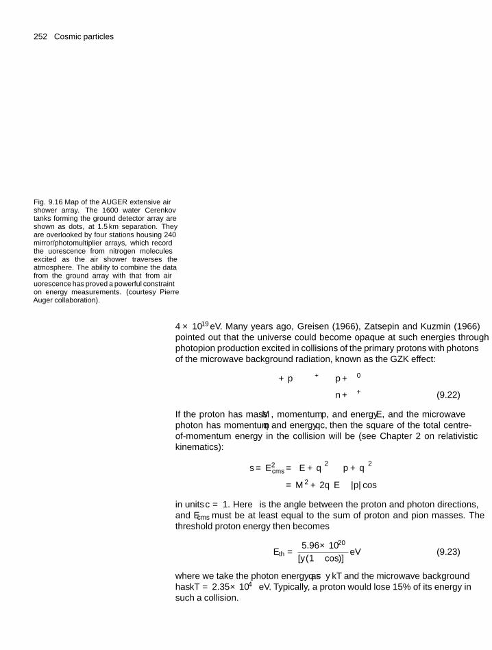
252 Cosmic particles
Fig. 9.16 Map of the AUGER extensive airshower array. The 1600 water Cerenkovtanks forming the ground detector array areshown as dots, at 1.5 km separation. Theyare overlooked by four stations housing 240mirror/photomultiplier arrays, which recordthe fluorescence from nitrogen moleculesexcited as the air shower traverses theatmosphere. The ability to combine the datafrom the ground array with that from airfluorescence has proved a powerful constrainton energy measurements. (courtesy PierreAuger collaboration).
4 × 10¹⁹ eV. Many years ago, Greisen (1966), Zatsepin and Kuzmin (1966)pointed out that the universe could become opaque at such energies throughphotopion production excited in collisions of the primary protons with photonsof the microwave background radiation, known as the GZK effect:
γ + p → �+ → p + π0
→ n + π+ (9.22)
If the proton has mass M , momentum p, and energy E, and the microwavephoton has momentum q and energy qc, then the square of the total centre-of-momentum energy in the collision will be (see Chapter 2 on relativistickinematics):
s = E2cms = (E + q
)2 − (p + q)2
= M 2 + 2q(E − |p| cos θ
)in units c = 1. Here θ is the angle between the proton and photon directions,and Ecms must be at least equal to the sum of proton and pion masses. Thethreshold proton energy then becomes
Eth = 5.96 × 10²⁰
[y(1 − cos θ)]eV (9.23)
where we take the photon energy as q = y kT and the microwave backgroundhas kT = 2.35 × 10⁻⁴ eV. Typically, a proton would lose 15% of its energy insuch a collision.
9.14 Radio galaxies and quasars 253
As an example, for head-on collisions (cos θ = −1) and y = 5, Eth =6 × 10¹⁹ eV. The cross-section for the reaction (9.22) near threshold isσ = 2 × 10⁻²⁸ cm2, and the total microwave photon density is ρ =400 cm−3, giving a collision mean free path λ = 1/ρσ = 4.1 Mpc forall the microwave photons. For the 10% of photons with y > 5 the meanfree path would be of order 50 Mpc. So one can expect that protons ofE > Eth coming from beyond the local galactic supercluster would havetheir energies attenuated by collisions with the microwave background (seeTable 5.1 for distance scales). In fact detailed calculations (Dermer 2007)show that indeed the flux above about 5 × 10¹⁹ eV should fall off sharply,as seems to be found in the HiRes and AUGER experiments—see (9.2) andFig. 9.3(c). The AUGER results on shower profiles indicate that many of thehighest energy primary particles are heavy nuclei, for which the dominantenergy loss mechanism would be photonuclear disintegration by CMB photons.It turns out however that the expected cut-off energy is comparable to that for theprotons.
It is believed that the ‘ankle’effect, that is, the slight flattening of the spectrumbetween 4 × 10¹⁸ eV and 4 × 10¹⁹ eV, may indicate the dominance of particleswhich are extra-galactic in origin. For a galactic magnetic field of order 3μ G(0.3 nT) the radius of curvature of protons of E = 4×10¹⁸ eV is ∼ 4 kpc. Suchparticles would not be trapped in the magnetic fields of a spiral galaxy, with adisc thickness an order of magnitude less than this.
9.13 Point sources of ultra-high-energycosmic rays
There is in general no correlation between the directions of high-energy(charged) cosmic ray primaries and point sources. Except at the very highestenergies, any anisotropy would be destroyed by the galactic magnetic field.However, the AUGER experiment does find significant anisotropies for eventsabove 6 × 10¹⁹ eV (Abraham et al. 2007). All 27 events above this limit arefound to lie inside a 3◦ cone towards a known AGN (located within 100 Mpcof the Earth). The probability that this could happen by chance is of order2 × 10−3. This evidence seems to indicate that the extreme energy cosmic raysare accelerated by a mechanism associated with massive black holes. Of course,the fact that such correlations are possible implies that the net magnetic fieldsin deep space beyond 10 Mpc must be extremely weak, less than about 10−11 G(see also Section 8.2).
9.14 Radio galaxies and quasars
The electromagnetic radiation from a galaxy such as the Milky Wayencompasses a vast spectral range, from radio wavelengths (centimetres tokilometres) to γ-rays with energies up to many TeV. In our own galaxy, less than
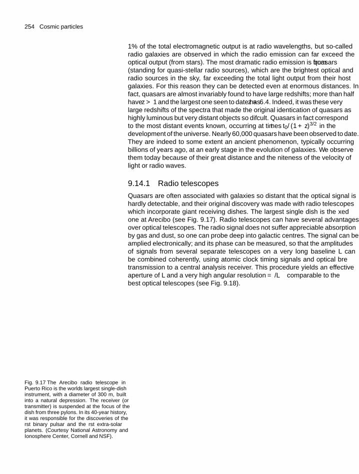
254 Cosmic particles
1% of the total electromagnetic output is at radio wavelengths, but so-calledradio galaxies are observed in which the radio emission can far exceed theoptical output (from stars). The most dramatic radio emission is from quasars(standing for quasi-stellar radio sources), which are the brightest optical andradio sources in the sky, far exceeding the total light output from their hostgalaxies. For this reason they can be detected even at enormous distances. Infact, quasars are almost invariably found to have large redshifts; more than halfhave z > 1 and the largest one seen to date has z = 6.4. Indeed, it was these verylarge redshifts of the spectra that made the original identification of quasars ashighly luminous but very distant objects so difficult. Quasars in fact correspondto the most distant events known, occurring at times t ∼ t0/(1 + z)3/2 in thedevelopment of the universe. Nearly 60,000 quasars have been observed to date.They are indeed to some extent an ancient phenomenon, typically occurringbillions of years ago, at an early stage in the evolution of galaxies. We observethem today because of their great distance and the finiteness of the velocity oflight or radio waves.
9.14.1 Radio telescopes
Quasars are often associated with galaxies so distant that the optical signal ishardly detectable, and their original discovery was made with radio telescopeswhich incorporate giant receiving dishes. The largest single dish is the fixedone at Arecibo (see Fig. 9.17). Radio telescopes can have several advantagesover optical telescopes. The radio signal does not suffer appreciable absorptionby gas and dust, so one can probe deep into galactic centres. The signal can beamplified electronically; and its phase can be measured, so that the amplitudesof signals from several separate telescopes on a very long baseline L canbe combined coherently, using atomic clock timing signals and optical fibretransmission to a central analysis receiver. This procedure yields an effectiveaperture of L and a very high angular resolution �θ = λ/L comparable to thebest optical telescopes (see Fig. 9.18).
Fig. 9.17 The Arecibo radio telescope inPuerto Rico is the world’s largest single-dishinstrument, with a diameter of 300 m, builtinto a natural depression. The receiver (ortransmitter) is suspended at the focus of thedish from three pylons. In its 40-year history,it was responsible for the discoveries of thefirst binary pulsar and the first extra-solarplanets. (Courtesy National Astronomy andIonosphere Center, Cornell and NSF).
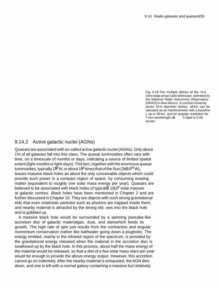
9.14 Radio galaxies and quasars 255
Fig. 9.18 The multiple dishes of the VLA(very large array) radio telescope, operated bythe National Radio Astronomy Observatory(NRAO) in New Mexico. It consists of twentyseven 25 m diameter dishes, which can beoperated as an interferometer with a baselineL up to 36 km, and an angular resolution for7 mm wavelength of λ/L ∼ 0.2 μrad or 0.05arcsec.
9.14.2 Active galactic nuclei (AGNs)
Quasars are associated with so-called active galactic nuclei (AGNs). Only about1% of all galaxies fall into this class. The quasar luminosities often vary withtime, on a timescale of months or days, indicating a source of limited spatialextent (light-months or light-days). This fact, together with the enormous quasarluminosities, typically 1040 W, or about 1013 times that of the Sun (3.9×1026 W),leaves massive black holes as about the only conceivable objects which couldprovide such power in a compact region of space, by consuming inflowingmatter (equivalent to roughly one solar mass energy per year). Quasars arebelieved to be associated with black holes of typically 106 − 109 solar massesat galactic centres. Black holes have been mentioned in Chapter 2 and arefurther discussed in Chapter 10. They are objects with such strong gravitationalfields that even relativistic particles such as photons are trapped inside them,and nearby material is attracted by the strong field, flows into the black holeand is gobbled up.
A massive black hole would be surrounded by a spinning pancake-likeaccretion disc of galactic material—gas, dust, and stars—which feeds itsgrowth. The high rate of spin just results from the contraction and angularmomentum conservation (rather like bathwater going down a plughole). Theenergy emitted, mainly in the infrared region of the spectrum, is provided bythe gravitational energy released when the material in the accretion disc isswallowed up by the black hole. In this process, about half the mass energy ofthe material would be released, so that a diet of a few solar mass stars per yearwould be enough to provide the above energy output. However, this accretioncannot go on indefinitely. After the nearby material is exhausted, the AGN diesdown, and one is left with a normal galaxy containing a massive but relatively
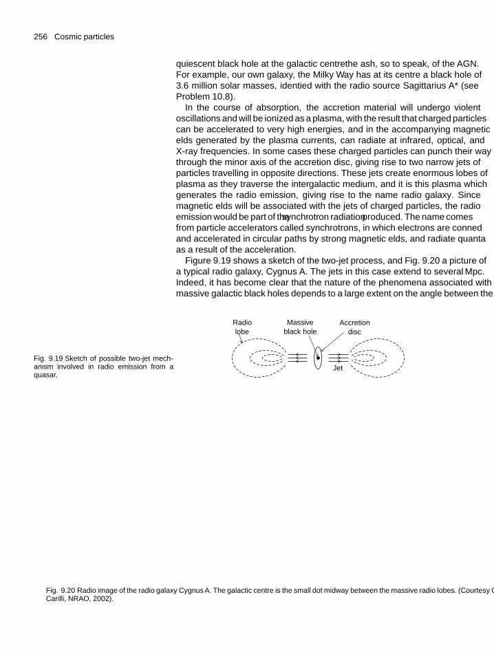
256 Cosmic particles
quiescent black hole at the galactic centre—the ash, so to speak, of the AGN.For example, our own galaxy, the Milky Way has at its centre a black hole of3.6 million solar masses, identified with the radio source Sagittarius A* (seeProblem 10.8).
In the course of absorption, the accretion material will undergo violentoscillations and will be ionized as a plasma, with the result that charged particlescan be accelerated to very high energies, and in the accompanying magneticfields generated by the plasma currents, can radiate at infrared, optical, andX-ray frequencies. In some cases these charged particles can punch their waythrough the minor axis of the accretion disc, giving rise to two narrow jets ofparticles travelling in opposite directions. These jets create enormous lobes ofplasma as they traverse the intergalactic medium, and it is this plasma whichgenerates the radio emission, giving rise to the name ‘radio galaxy’. Sincemagnetic fields will be associated with the jets of charged particles, the radioemission would be part of the synchrotron radiation produced. The name comesfrom particle accelerators called synchrotrons, in which electrons are confinedand accelerated in circular paths by strong magnetic fields, and radiate quantaas a result of the acceleration.
Figure 9.19 shows a sketch of the two-jet process, and Fig. 9.20 a picture ofa typical radio galaxy, Cygnus A. The jets in this case extend to several Mpc.Indeed, it has become clear that the nature of the phenomena associated withmassive galactic black holes depends to a large extent on the angle between the
Fig. 9.19 Sketch of possible two-jet mech-anism involved in radio emission from aquasar.
Radiolobe
Accretiondisc
Massiveblack hole
Jet
Fig. 9.20 Radio image of the radio galaxy Cygnus A. The galactic centre is the small dot midway between the massive radio lobes. (Courtesy ChrisCarilli, NRAO, 2002).
9.15 Atmospheric neutrinos: neutrino oscillations 257
jet axis and the line of sight to the Earth. If it is large, one obtains two jets ofcomparable size as in Fig. 9.20 in the case of Cygnus A. However, if the jetvelocities are extreme relativistic and the angle happens to be small, so that onejet is approaching and the other is receding, the Doppler shift of the frequencycan mean that the approaching jet is very bright while the receding one is belowthe threshold for detection. There are many interesting effects associated withthe jets. For example, the observed transverse velocity may apparently exceedlight velocity (see Problem 9.13). As another example, if the photons observedare of high energy, they would have been radiated by electrons of very largeLorentz factor γ , and hence are confined to a narrow angular spread of order1/γ (see Problem 2.5). Thus small fluctuations in the jet angle could deflect thebeam away from the observer, and the observed intensity could vary on shorttimescales. This may be a possible cause of the extreme variability of some ofthe γ-ray sources.
Two-jet phenomena, on a much smaller scale, and termed microquasars havealso been observed in local galaxies. These are assumed to be due to black holesof order a few solar masses only, with accretion from a nearby companion star.The distance scale of the radio lobes is of order parsec in this case, rather thanthe megaparsec scale of quasars.
AGN sources from which the γ-ray emission is in the TeV energy region,are referred to as blazars, the most famous example being Markarian 501(see Fig 9.13). From this source the γ-ray flux can vary by an order of magnitudefrom night to night, and during the year 1997 it increased by a factor 50.
9.14.3 The Lyman α forest
Before leaving the subject of quasars, we refer briefly to their role in establishingthe degree of re-ionization of the stellar medium, consequent on the appearanceof the first stars. As discussed in the next chapter, stars are believed to havestarted to form at redshift z < 12, and their ultraviolet emissions wouldhave caused re-ionization of the, previously neutral, interstellar hydrogen. Thedegree of ionization can be estimated from observations of the so-called Lymanα forest. This arises from clouds of hydrogen when they are backlit by the intenselight from a quasar. Let us recall that the Lyman series in the hydrogen atomconsists of spectral lines of wavelength λ = (2h/α2mec
) [(1/n1)
2 − (1/n2)2]
for transitions between principal quantum numbers n1 = 1 and n2 > 1. TheLyman α line, for n2 = 2, has λ = 121.6 nm, while the ‘Lyman limit’, forn2 = ∞, has λ = 91.0 nm. Passage of light from the quasar through anyneutral hydrogen will show a ‘forest’ of absorption lines between these twowavelengths. Figure 9.21 shows a typical quasar spectrum (corrected for anyredshift). From analysis of the line shapes and intensities it is then possible todeduce the fraction of hydrogen which is neutral, that is, not ionized. It is smallbut not negligible.
9.15 Atmospheric neutrinos: neutrino oscillations
Neutrinos and antineutrinos are constituents of the secondary cosmic raysgenerated in the Earth’s atmosphere by interactions of the primary particles,
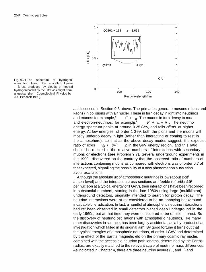
258 Cosmic particles
Fig. 9.21 The spectrum of hydrogenabsorption lines, the so-called Lymanα forest produced by clouds of neutralhydrogen backlit by the ultraviolet light froma quasar (from ‘Cosmological Physics’ byJ.A. Peacock 1999).
0100 120
Rest wavelength/nm
140
0.5
Flux
(l
f l)
1Q0201 + 113
Ly limit D Lya
CIV
z = 3.638
↑
↑↑
↑
as discussed in Section 9.5 above. The primaries generate mesons (pions andkaons) in collisions with air nuclei. These in turn decay in flight into neutrinosand muons: for example, π+ → μ+ + νμ. The muons in turn decay to muon-and electron-neutrinos: for example, μ+ → e+ + ve + vμ. The neutrinoenergy spectrum peaks at around 0.25 GeV, and falls off as E−2.7 at higherenergy. At low energies, of order 1 GeV, both the pions and the muons willmostly undergo decay in flight (rather than interacting or coming to rest inthe atmosphere), so that as the above decay modes suggest, the expectedratio of fluxes φ
(vμ
)/φ (ve) ≈ 2 in the GeV energy region, and this ratio
should be reflected in the relative numbers of interactions with secondarymuons or electrons (see Problem 9.7). Several underground experiments inthe 1990s discovered on the contrary that the observed ratio of numbers ofinteractions containing muons as compared with electrons was of order 0.7 ofthat expected, signalling the possibility of a new phenomenon such as neutrinoflavour oscillations.
Although the absolute flux of atmospheric neutrinos is low (about 1 cm−2s−1
at sea-level) and the interaction cross-sections are feeble (of order 10−38 cm2
per nucleon at a typical energy of 1 GeV), their interactions have been recordedin substantial numbers, starting in the late 1980s using large (multikiloton)underground detectors, originally intended to search for proton decay. Theneutrino interactions were at first considered to be an annoying backgroundincapable of eradication. In fact, a handful of atmospheric neutrino interactionshad first been observed in small detectors placed deep underground in theearly 1960s, but at that time they were considered to be of little interest. Sothe discovery of neutrino oscillations with atmospheric neutrinos, like manyother discoveries in science, has been largely accidental, as a by-product of aninvestigation which failed in its original aim. By good fortune it turns out thatthe typical energies of atmospheric neutrinos, of order 1 GeV and determinedby the effect of the Earth’s magnetic field on the primary cosmic ray nuclei,combined with the accessible neutrino path lengths, determined by the Earth’sradius, are exactly matched to the relevant scale of neutrino mass differences.As indicated in Chapter 4, there are three neutrino flavours (νe, νμ, and ντ) and
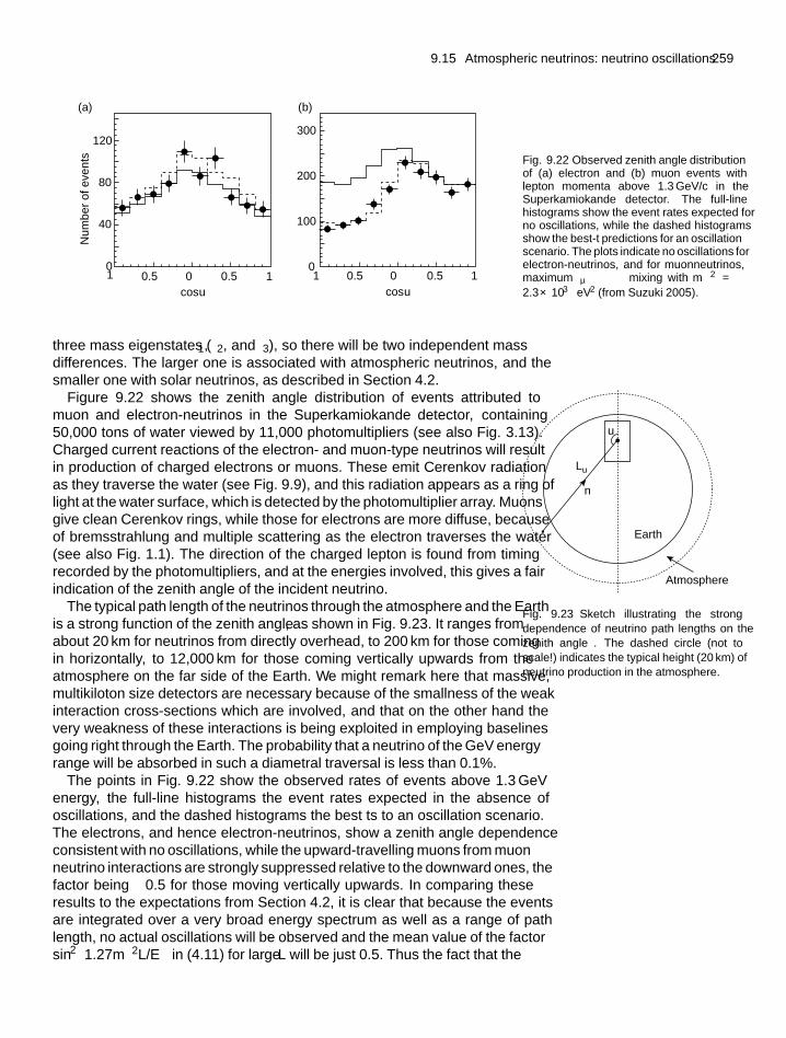
9.15 Atmospheric neutrinos: neutrino oscillations 259
120
80
40
0
Num
ber
of e
vent
s
–1
300
200
100
0–1–0.5 0 0.5 1
cos u
–0.5 0 0.5 1cos u
(a) (b)
Fig. 9.22 Observed zenith angle distributionof (a) electron and (b) muon events withlepton momenta above 1.3 GeV/c in theSuperkamiokande detector. The full-linehistograms show the event rates expected forno oscillations, while the dashed histogramsshow the best-fit predictions for an oscillationscenario. The plots indicate no oscillations forelectron-neutrinos, and for muon–neutrinos,maximum νμ → ντ mixing with �m2 =2.3 × 10⁻³ eV2 (from Suzuki 2005).
three mass eigenstates (ν1, ν2, and ν3), so there will be two independent massdifferences. The larger one is associated with atmospheric neutrinos, and thesmaller one with solar neutrinos, as described in Section 4.2.
Figure 9.22 shows the zenith angle distribution of events attributed tomuon and electron-neutrinos in the Superkamiokande detector, containing50,000 tons of water viewed by 11,000 photomultipliers (see also Fig. 3.13).Charged current reactions of the electron- and muon-type neutrinos will resultin production of charged electrons or muons. These emit Cerenkov radiationas they traverse the water (see Fig. 9.9), and this radiation appears as a ring oflight at the water surface, which is detected by the photomultiplier array. Muonsgive clean Cerenkov rings, while those for electrons are more diffuse, becauseof bremsstrahlung and multiple scattering as the electron traverses the water(see also Fig. 1.1). The direction of the charged lepton is found from timingrecorded by the photomultipliers, and at the energies involved, this gives a fairindication of the zenith angle of the incident neutrino.
Lu
Earth
Atmosphere
u
n
Fig. 9.23 Sketch illustrating the strongdependence of neutrino path lengths on thezenith angle θ. The dashed circle (not toscale!) indicates the typical height (20 km) ofneutrino production in the atmosphere.
The typical path length of the neutrinos through the atmosphere and the Earthis a strong function of the zenith angle θ, as shown in Fig. 9.23. It ranges fromabout 20 km for neutrinos from directly overhead, to 200 km for those comingin horizontally, to 12,000 km for those coming vertically upwards from theatmosphere on the far side of the Earth. We might remark here that massive,multikiloton size detectors are necessary because of the smallness of the weakinteraction cross-sections which are involved, and that on the other hand thevery weakness of these interactions is being exploited in employing baselinesgoing right through the Earth. The probability that a neutrino of the GeV energyrange will be absorbed in such a diametral traversal is less than 0.1%.
The points in Fig. 9.22 show the observed rates of events above 1.3 GeVenergy, the full-line histograms the event rates expected in the absence ofoscillations, and the dashed histograms the best fits to an oscillation scenario.The electrons, and hence electron-neutrinos, show a zenith angle dependenceconsistent with no oscillations, while the upward-travelling muons from muon–neutrino interactions are strongly suppressed relative to the downward ones, thefactor being ≈ 0.5 for those moving vertically upwards. In comparing theseresults to the expectations from Section 4.2, it is clear that because the eventsare integrated over a very broad energy spectrum as well as a range of pathlength, no actual oscillations will be observed and the mean value of the factorsin2 (1.27�m2L/E
)in (4.11) for large L will be just 0.5. Thus the fact that the
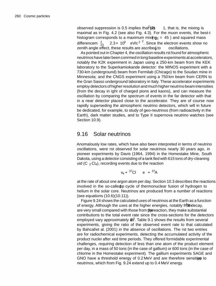
260 Cosmic particles
observed suppression is 0.5 implies that sin2(2θ) ≈ 1, that is, the mixing ismaximal as in Fig. 4.2 (see also Fig. 4.3). For the muon events, the best-fithistogram corresponds to a maximum mixing (θ23 = 45◦) and squared mass
difference �m223 ≈ 2.3 × 10⁻³
(eV/c2
)2. Since the electron events show no
zenith angle effect, these results are ascribed to νμ → ντ oscillations.As pointed out in Chapter 4, the oscillation results first found for atmospheric
neutrinos have later been confirmed in long baseline experiments at accelerators,notably the K2K experiment in Japan using a 250-km beam from the KEKlaboratory to the Superkamiokande detector: the MINOS experiment with a730-km (underground) beam from Fermilab (Chicago) to the Soudan mine inMinnesota; and the CNGS experiment using a 750 km beam from CERN tothe Gran Sasso underground laboratory in Italy. These accelerator experimentsemploy detectors of higher resolution and much higher neutrino beam intensities(from the decay in flight of charged pions and kaons), and can measure theoscillation by comparing the spectrum of events in the far detector with thatin a near detector placed close to the accelerator. They are of course nowrapidly superseding the atmospheric neutrino detectors, which will in futurebe dedicated, for example, to study of geo-neutrinos (from radioactivity in theEarth), dark matter studies, and to Type II supernova neutrino watches (seeSection 10.9).
9.16 Solar neutrinos
Anomalously low rates, which have also been interpreted in terms of neutrinooscillations, were first observed for solar neutrinos nearly 30 years ago, inpioneer experiments by Davis (1964, 1994) in the Homestake Mine, SouthDakota, using a detector consisting of a tank filled with 615 tons of dry-cleaningfluid (C2 Cl4), recording events due to the reaction
ve + 37Cl → e− + 37A
at the rate of about one argon atom per day. Section 10.3 describes the reactionsinvolved in the so-called pp cycle of thermonuclear fusion of hydrogen tohelium in the solar core. Neutrinos are produced from a number of reactions(see equations (10.6)–(10.11)).
Figure 9.24 shows the calculated fluxes of neutrinos at the Earth as a functionof energy. Although the fluxes at the higher energies, notably from 8B decay,are very small compared with those from the pp reaction, they make substantialcontributions to the total event rate since the cross-sections for the detectorsemployed vary approximately as E3
ν . Table 9.1 shows the results from severalexperiments, giving the ratio of the observed event rate to that calculatedby Bahcall et al. (2001) in the absence of oscillations. The first two entriesare for radiochemical experiments, detecting the accumulated activity of theproduct nuclei after fixed time periods. They offered formidable experimentalchallenges, requiring detection of less than one atom of the product elementper day, in a mass of 50 tons (in the case of gallium) or 600 tons (in the case ofchlorine in the Homestake experiment). The gallium experiments SAGE andGNO have a threshold energy of 0.2 MeV and are therefore sensitive to ppneutrinos, which from Fig. 9.24 extend up to 0.4 MeV energy.
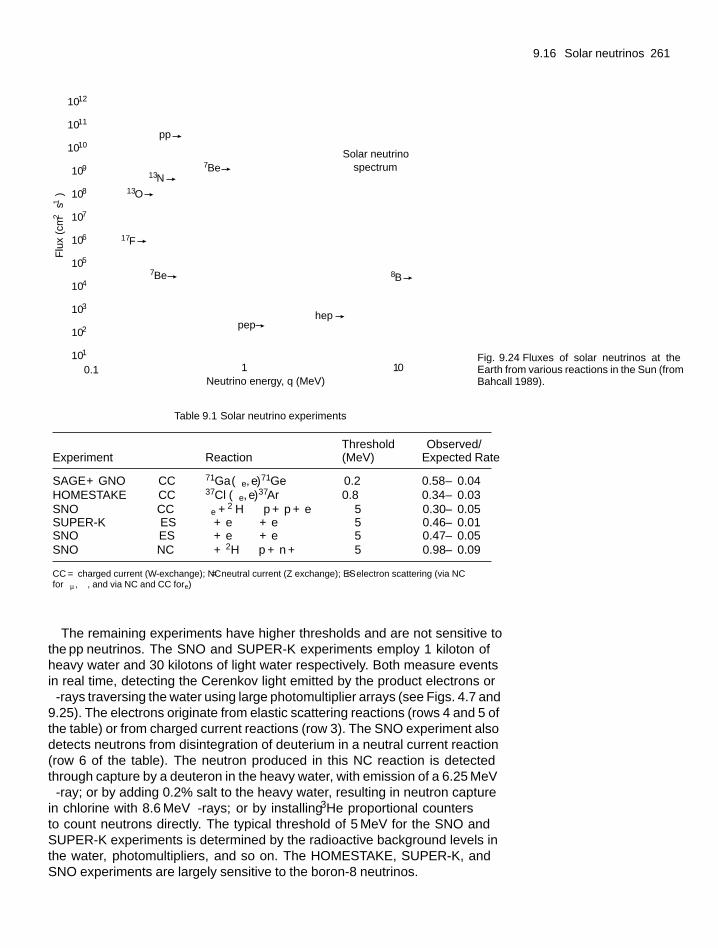
9.16 Solar neutrinos 261
1012
1011
1010
109
108
107
106
105
Flux
(cm
–2 s
–1)
104
103
102
101
0.1
pp
pephep
7Be
7Be 8B
17F
13O
13N
1 10
Solar neutrinospectrum
Neutrino energy, q (MeV)
Fig. 9.24 Fluxes of solar neutrinos at theEarth from various reactions in the Sun (fromBahcall 1989).
Table 9.1 Solar neutrino experiments
Threshold Observed/Experiment Reaction (MeV) Expected Rate
SAGE + GNO CC 71Ga (νe, e)71Ge 0.2 0.58 ± 0.04HOMESTAKE CC 37Cl (νe, e)37Ar 0.8 0.34 ± 0.03SNO CC νe +2 H → p + p + e ∼ 5 0.30 ± 0.05SUPER-K ES ν + e → ν + e ∼ 5 0.46 ± 0.01SNO ES ν + e → ν + e ∼ 5 0.47 ± 0.05SNO NC ν + 2H → p + n + ν ∼ 5 0.98 ± 0.09
CC = charged current (W-exchange); NC = neutral current (Z exchange); ES = electron scattering (via NCfor νμ, ντ , and via NC and CC for νe)
The remaining experiments have higher thresholds and are not sensitive tothe pp neutrinos. The SNO and SUPER-K experiments employ 1 kiloton ofheavy water and 30 kilotons of light water respectively. Both measure eventsin real time, detecting the Cerenkov light emitted by the product electrons orγ-rays traversing the water using large photomultiplier arrays (see Figs. 4.7 and9.25). The electrons originate from elastic scattering reactions (rows 4 and 5 ofthe table) or from charged current reactions (row 3). The SNO experiment alsodetects neutrons from disintegration of deuterium in a neutral current reaction(row 6 of the table). The neutron produced in this NC reaction is detectedthrough capture by a deuteron in the heavy water, with emission of a 6.25 MeVγ-ray; or by adding 0.2% salt to the heavy water, resulting in neutron capturein chlorine with 8.6 MeV γ-rays; or by installing 3He proportional countersto count neutrons directly. The typical threshold of 5 MeV for the SNO andSUPER-K experiments is determined by the radioactive background levels inthe water, photomultipliers, and so on. The HOMESTAKE, SUPER-K, andSNO experiments are largely sensitive to the boron-8 neutrinos.
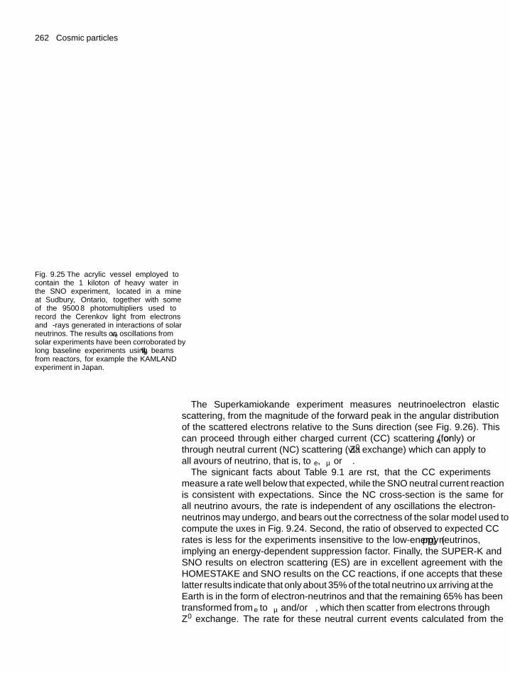
262 Cosmic particles
Fig. 9.25 The acrylic vessel employed tocontain the 1 kiloton of heavy water inthe SNO experiment, located in a mineat Sudbury, Ontario, together with someof the 9500 8′′ photomultipliers used torecord the Cerenkov light from electronsand γ-rays generated in interactions of solarneutrinos. The results on ve oscillations fromsolar experiments have been corroborated bylong baseline experiments using ve beamsfrom reactors, for example the KAMLANDexperiment in Japan.
The Superkamiokande experiment measures neutrino–electron elasticscattering, from the magnitude of the forward peak in the angular distributionof the scattered electrons relative to the Sun’s direction (see Fig. 9.26). Thiscan proceed through either charged current (CC) scattering (for νe only) orthrough neutral current (NC) scattering (via Z0 exchange) which can apply toall flavours of neutrino, that is, to νe, νμ or ντ .
The significant facts about Table 9.1 are first, that the CC experimentsmeasure a rate well below that expected, while the SNO neutral current reactionis consistent with expectations. Since the NC cross-section is the same forall neutrino flavours, the rate is independent of any oscillations the electron-neutrinos may undergo, and bears out the correctness of the solar model used tocompute the fluxes in Fig. 9.24. Second, the ratio of observed to expected CCrates is less for the experiments insensitive to the low-energy (pp) neutrinos,implying an energy-dependent suppression factor. Finally, the SUPER-K andSNO results on electron scattering (ES) are in excellent agreement with theHOMESTAKE and SNO results on the CC reactions, if one accepts that theselatter results indicate that only about 35% of the total neutrino flux arriving at theEarth is in the form of electron-neutrinos and that the remaining 65% has beentransformed from νe to νμ and/or ντ , which then scatter from electrons throughZ0 exchange. The rate for these neutral current events calculated from the
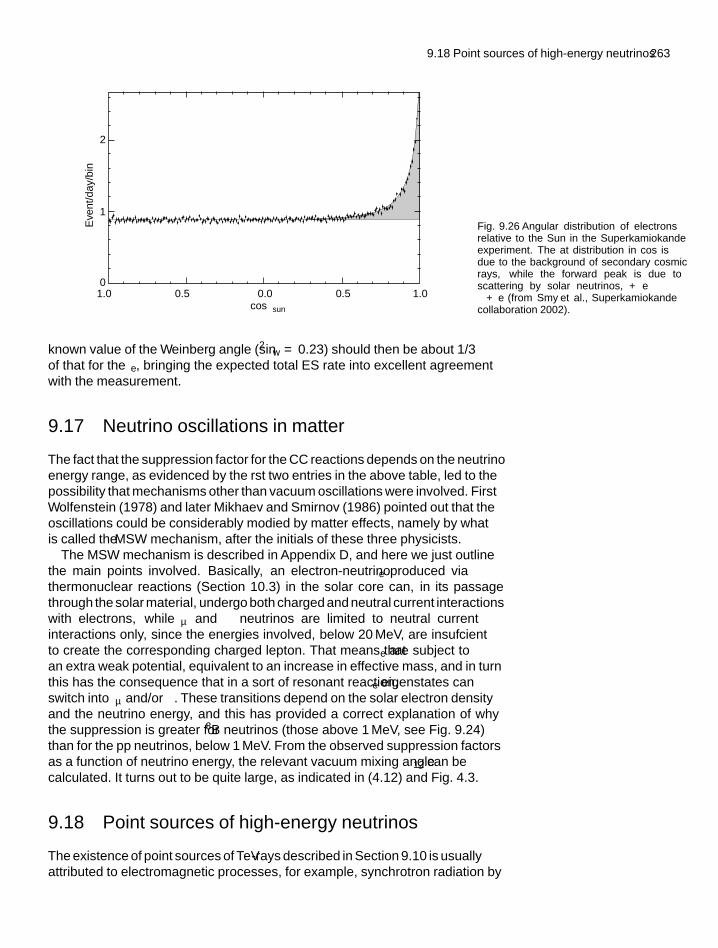
9.18 Point sources of high-energy neutrinos 263
–1.00
1
Eve
nt/d
ay/b
in
2
0.0cos �sun
–0.5 0.5 1.0
Fig. 9.26 Angular distribution of electronsrelative to the Sun in the Superkamiokandeexperiment. The flat distribution in cos θ isdue to the background of secondary cosmicrays, while the forward peak is due toscattering by solar neutrinos, ν + e →ν + e (from Smy et al., Superkamiokandecollaboration 2002).
known value of the Weinberg angle (sin2 θw = 0.23) should then be about 1/3of that for the νe, bringing the expected total ES rate into excellent agreementwith the measurement.
9.17 Neutrino oscillations in matter
The fact that the suppression factor for the CC reactions depends on the neutrinoenergy range, as evidenced by the first two entries in the above table, led to thepossibility that mechanisms other than vacuum oscillations were involved. FirstWolfenstein (1978) and later Mikhaev and Smirnov (1986) pointed out that theoscillations could be considerably modified by matter effects, namely by whatis called the MSW mechanism, after the initials of these three physicists.
The MSW mechanism is described in Appendix D, and here we just outlinethe main points involved. Basically, an electron-neutrino νe produced viathermonuclear reactions (Section 10.3) in the solar core can, in its passagethrough the solar material, undergo both charged and neutral current interactionswith electrons, while νμ and ντ neutrinos are limited to neutral currentinteractions only, since the energies involved, below 20 MeV, are insufficientto create the corresponding charged lepton. That means that νe are subject toan extra weak potential, equivalent to an increase in effective mass, and in turnthis has the consequence that in a sort of resonant reaction, νe eigenstates canswitch into νμ and/or ντ . These transitions depend on the solar electron densityand the neutrino energy, and this has provided a correct explanation of whythe suppression is greater for 8B neutrinos (those above 1 MeV, see Fig. 9.24)than for the pp neutrinos, below 1 MeV. From the observed suppression factorsas a function of neutrino energy, the relevant vacuum mixing angle θ12 can becalculated. It turns out to be quite large, as indicated in (4.12) and Fig. 4.3.
9.18 Point sources of high-energy neutrinos
The existence of point sources of TeVγ-rays described in Section 9.10 is usuallyattributed to electromagnetic processes, for example, synchrotron radiation by
264 Cosmic particles
high-energy electrons accelerated in the source. However, it is also possiblethat γ-rays could be produced by pion production and decay, π0 → 2γ , andthis would then imply high-energy neutrino point sources via π± → μ± + νμ.Such neutrinos could be detected in underground experiments via the secondarycharged muons they produce. At TeV energies, the muon range in rockwould be measured in kilometres, and the object would be to detect muonstravelling upwards (since any downward flux would be completely swampedby atmospheric muons from pion decay in the atmosphere overhead). Becauseof the high energy, the direction of the secondary muon will follow ratherclosely that of the parent neutrino. Here the very weakness of their interactionsis being exploited to detect neutrinos which have come up through the Earth andproduced a signal free of background, except for the ubiquitous atmosphericneutrinos, which are, however, broadly distributed in angle.
The rate of such neutrino events (compared with that of γ-rays) is expected tobe low on account of the weak cross-section. However, this is compensated, firstby the fact that the cross-section for the interaction of a neutrino with a quarkin the target nucleus rises as the square of the CMS energy, or linearly with thelaboratory neutrino energy (see (1.27)); and that in the neutrino-quark collision,the secondary muon energy, and hence its range in rock, is also proportionalto neutrino energy. So although the neutrino flux falls off rapidly with energy,it has to be multiplied by a factor of E2
ν to get the event rate. This argumentholds up to TeV energies, but beyond that, the cross-sections flatten off becauseof the W propagator in (1.9), and the muon range is no longer proportional toenergy because of radiation losses analogous to those of electrons discussedin Section 9.6, but coming in at a much higher energy (by a factor oforder
(mμ/me
)2).
The detection of rare high-energy cosmic neutrino interactions via thesecondary upward-travelling muons has to be carried out on a large scale, anduses great depths of sea water or of ice, and again relies on the detection of theCerenkov light radiated by the muon. Figure 9.27 shows one such experiment,in which strings of photomultipliers collect the Cerenkov signals over a volumewith dimensions of order several hundred meters. They have of course recordedatmospheric neutrino events, but so far no evidence for high-energy neutrinopoint sources. These arrays may also detect high-energy neutrinos from possibleWIMP–antiWIMP annihilations in the Sun (see Section 7.9).
9.19 Gravitational radiation
Of all the radiations incident upon the Earth from the cosmos, the mostelusive and most difficult to detect is surely gravitational radiation. The keyequations describing gravitational radiation, its production and detection arefound from the general theory of relativity, which is outside the scope of thistext. Nevertheless, we can understand many of the features of gravity wavesby using the analogy with electromagnetic radiation.
First of all, we remark that in scattering problems it is usual to expandthe function describing a plane wave into a superposition of spherical waveswith different values of the orbital angular momentum, l, with respect to thescattering centre. An oscillation can equally be represented in the form ofa multipole expansion, corresponding to a superposition of oscillators with

9.19 Gravitational radiation 265
30 m
Ice surface level
190 m
380 m
1000 m
1950 m
60 m35 m
1520 m
810 m
Depths
Fig. 9.27 Diagram of the strings ofphotomultipliers sunk in ice at the South Polein the AMANDA experiment. They recordCerenkov light emitted by upward comingmuons generated in neutrino interactions.Timing provides information on the zenithand azimuthal angles of the muon. TheAMANDA array is currently being replacedby a much larger array, ICECUBE, covering1 km3 volume.
+q
+q
+q
+q +q–q
–q
–q
–q –q(a) (b)
(c) Fig. 9.28 (a) an electric dipole. (b) and (c)two configurations of an electric quadrupole,for which the dipole moment is zero.
266 Cosmic particles
different l-values. Thus dipole, quadrupole, sextupole, … oscillator terms areassociated with l = 1, 2, 3, . . . waves. Figure 9.28 depicts a simple electricdipole and two versions of an electric quadrupole. If ω represents the angularfrequency of the oscillation, the power radiated is given by the formula
P (l) = 2cF (l)(ω
c
)2l+2 |Qlm|2 (9.24)
where F (l) = (l + 1)/[l {(2l + 1)!!}2
]. Here n!! = 1.3.5.7. . .—and Qlm is the
l th moment of the distribution of electric charge density ρ, integrated overvolume and projected along the z-axis, along which m is the component ofangular momentum:
Qlm =∫
rl Y ∗lm (θ, φ) ρ dV (9.25)
Here Ylm(θ, φ) is a spherical harmonic. In order of magnitude, an electric dipolemoment (l = 1) has Q1 ∼ er where r is the dimension of the system and edenotes the charge. Thus from (9.24) the power radiated is of order
Pdipole ∼ ω4e2r2
c3(9.26)
The dependence on ω4 arises because the power radiated is proportional to thesquare of the acceleration of the charges, varying as ω2. The formula applies alsoto Rayleigh scattering of light by air molecules and by dust, and its dependenceon 1/λ4 accounts for the blueness of the sky and the redness of the sunset. Foran electric quadrupole moment (l = 2), Q2 ∼ er2 and the power radiated is oforder
Pquadrupole ∼ ω6e2r4
c5(9.27)
The gravitational field is a tensor field (as compared with the vector, spin 1photon field of electromagnetism), and gravitational interactions are mediatedby gravitons of spin 2. As a result, dipole emission of gravitational waves isimpossible and the simplest radiator of gravitational waves is an oscillatingmass quadrupole. The power emitted can be estimated by replacing e2 inthe expression e2/r for the electric potential between charges by GM 2 in theexpression GM 2/r for the gravitational potential between masses, so that
Pgrav ∼ ω6GM 2r4
c5(9.28)
Here, M denotes a typical mass and r a typical dimension in the quadrupolesystem, and we have just quoted the order of magnitude result for orientation.It should be emphasised that a quantitative calculation using Newtonianmechanics and simply substituting from the electric quadrupole formula will inany case underestimate the power in gravitational radiation, as computed usingthe general theory of relativity, by a factor 4. We quote here two examplesof quantitative predictions. A rod of length L and mass M rotating about its
9.20 The binary pulsar 267
mid-point with angular velocity ω emits gravitational radiation with the power
P =(
2
45
)ω6GM 2 L4
c5(9.29)
while a binary system consisting of two stars in a circular orbit of diameter Dand angular frequency ω radiates power
P =(
32
5
)ω6G μ2 D4
c5(9.30)
where μ is the reduced mass, and for stars of equal mass M , μ = M /2.For an experiment on a laboratory scale, we could take L ∼ 1 m, M ∼ 1 kg
and ω ∼ 103 s−1, which from (9.28) gives P ∼ 10−36 watts only. Accordingto (9.30), even the entire Earth, in its orbit around the Sun, radiates a mere 196watts. More likely objects for a measurable level of gravitational radiation maybe binary stars in a late stage of evolution, just as they coalesce to black holes,when a considerable fraction of the rest energy of the stars should be emittedas gravitational radiation. Indeed, it is believed that gravitational energy lossis what leads to the collapse. Somewhat less dramatic is the radiation emittedduring the formation of a neutron star, which is followed by the spectacularoptical display of a Type II supernova (see Sections 10.8–10.10).
9.20 The binary pulsar
The most convincing evidence for the existence of gravitational radiation, andthrough it, a quantitative test of general relativity, came from the observationsof the binary pulsar PSR 1913+16 by Hulse and Taylor, first recorded in 1975.This binary consists of two neutron stars, of which one is a pulsar with a periodof 0.059 s. Pulsars are neutron stars (see Section 10.10) which spin rapidly withfrequencies of 10–100 s−1, emitting radio waves in a beam which periodicallysweep past the observer, like a rotating beam from a lighthouse. The orbitalperiod of this binary, τ = 7.8 h, and other characteristics of the orbit werefound from the Doppler shift of the pulsar signal as this neutron star circulatesits companion. The unique feature of this binary is that, during a period of morethan 20 years of observation, a tiny but steady decrease in the orbital period wasdetected. After a few minor corrections for galactic accelerations the observedfractional rate of decrease in the period τ was found to be:
dτ
dt= − (2.409 ± 0.005) × 10−12 (9.31)
Such a decrease is to be expected if the pair lose energy by emission ofgravitational radiation. To estimate the magnitude of this effect, let us assumefor simplicity that the two stars have equal masses M and execute a circularorbit of diameter D. With ω = 2π/τ as the angular frequency of the orbitalmotion, the tangential velocity of each star is v = ωD/2. The total energy of
268 Cosmic particles
the system is the sum of kinetic and potential energies:
Etot = 2 ×(
Mv2
2
)− GM 2
D(9.32)
Balancing the gravitational and centrifugal forces on one of the masses gives
2Mv2
D= GM 2
D2
so that
Etot = −GM 2
2D(9.33)
that is, the kinetic energy is just half the (absolute value of) the potentialenergy—another example of the virial theorem. Since from the above equationsEtot ∝ 1/D and ω ∝ 1/D3/2, the orbital period τ ∝ (Etot)
−3/2. Hence(1
τ
)dτ
dt= −
(3
2E
)dE
dt= −
(3
2
)P
E(9.34)
where P is the power radiated. The characteristics of the binary give ω =2.2 × 10⁻⁴, M ∼ 1.4 Msun. Inserting these values to obtain D and Etot, andusing (9.30) to estimate the power radiated, one obtains dτ/dt ∼ 10−13. Afull calculation, taking into account the eccentricity of the binary orbit and theinequality of the masses yields the result
dτ
dt= − (2.4025 ± 0.0002) × 10−12 (9.35)
agreeing exactly (within the 0.2% experimental error) with the observed value(9.31). This result has given great confidence that the basic physics is wellunderstood and that, despite enormous experimental difficulties, the detectionof gravitational radiation in the laboratory is worth pursuing.
Several such binary pulsars have now been observed. More remarkably, adouble pulsar, PSR J0737-3039 A and B, that is, a binary system in whichboth neutron stars A and B are pulsars, has been discovered (Lyne et al.2004). This system allows even more tests of general relativity, especially sincefortunately, the plane of the orbit practically coincides with the line of sight.First, the collapse of the orbit due to gravitational radiation was observed,again in agreement with the predictions from general relativity. Second, anorbital precession (Section 2.8) of 17◦ per year—about 100,000 times largerthan that for the orbit of the planet Mercury—was measured. The Shapiro delay(Section 2.7) in the signal was also detected as the beam from pulsar A passedclose by pulsar B. Finally, the gravitational time dilation was observed, thepulse rate from one pulsar slowing down as it passed closer to the other. Again,we should emphasise that these tests of general relativity are wonderful but forrelatively weak fields, far away from the non-linearities implied in the Einsteinfield equations for strong enough fields.
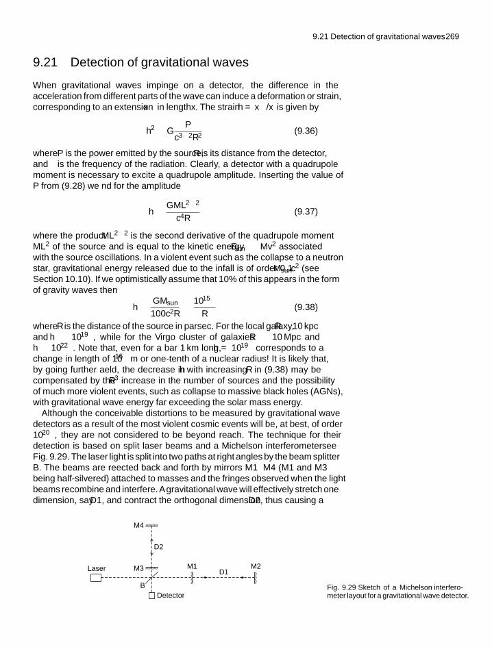
9.21 Detection of gravitational waves 269
9.21 Detection of gravitational waves
When gravitational waves impinge on a detector, the difference in theacceleration from different parts of the wave can induce a deformation or strain,corresponding to an extension �x in length x. The strain h = �x/x is given by
h2 ∼ GP
c3ω2R2(9.36)
where P is the power emitted by the source, R is its distance from the detector,and ω is the frequency of the radiation. Clearly, a detector with a quadrupolemoment is necessary to excite a quadrupole amplitude. Inserting the value ofP from (9.28) we find for the amplitude
h ∼ GML2ω2
c4R(9.37)
where the product ML2ω2 is the second derivative of the quadrupole momentML2 of the source and is equal to the kinetic energy Ekin ∼ Mv2 associatedwith the source oscillations. In a violent event such as the collapse to a neutronstar, gravitational energy released due to the infall is of order 0.1 Msunc2 (seeSection 10.10). If we optimistically assume that 10% of this appears in the formof gravity waves then
h ∼ GMsun
100 c2R∼ 10−15
R(9.38)
where R is the distance of the source in parsec. For the local galaxy, R ∼ 10 kpcand h ∼ 10−19, while for the Virgo cluster of galaxies R ∼ 10 Mpc andh ∼ 10−22. Note that, even for a bar 1 km long, h = 10−19 corresponds to achange in length of 10−16 m or one-tenth of a nuclear radius! It is likely that,by going further afield, the decrease in h with increasing R in (9.38) may becompensated by the R3 increase in the number of sources and the possibilityof much more violent events, such as collapse to massive black holes (AGNs),with gravitational wave energy far exceeding the solar mass energy.
Although the conceivable distortions to be measured by gravitational wavedetectors as a result of the most violent cosmic events will be, at best, of order10−20, they are not considered to be beyond reach. The technique for theirdetection is based on split laser beams and a Michelson interferometer—seeFig. 9.29. The laser light is split into two paths at right angles by the beam splitterB. The beams are reflected back and forth by mirrors M1 – M4 (M1 and M3being half-silvered) attached to masses and the fringes observed when the lightbeams recombine and interfere. Agravitational wave will effectively stretch onedimension, say D1, and contract the orthogonal dimension D2, thus causing a
M4
M3
Detector
Laser
D2
B
M1D1
M2
Fig. 9.29 Sketch of a Michelson interfero-meter layout for a gravitational wave detector.
270 Cosmic particles
fringe shift; alternatively, one can think of the gravitational wave as distortingthe space/time between the mirrors, thus introducing tiny (Shapiro) delays in therelative transit times of the light beams. A Fabry-Perot etalon is used so that thebeams make many traverses to and fro before recombining. As an example, thevalues chosen for the two LIGO experiments in the USA are D1, D2 ∼ 4 km,operating in a frequency range 10–1000 Hz, typical of the collapse times forneutron stars/black holes. In Europe, the dimensions of the VIRGO experimentare similar, while GEO600 is a smaller array with L = 0.6 km. All of theseexperiments have very comparable sensitivities, and all are extremely difficult,and require years of tuning before scientific runs can commence.
The main problems for these experiments are the effects of background(seismic) noise, which kills all hope of detecting a signal below about 10 Hz.The noise problem can be tackled to some extent by combining the signals fromtwo or more of the several detectors located in different positions worldwide,using timing information to reduce the noise and also indicate the direction ofthe source. For example, one of the LIGO and the TAMA (Japan) detectorshave operated in coincidence for almost 500 h and placed an upper limit onany signal of < 0.12 events per day (Abbott et al. 2006). The feasibilityof combining signals from all five of the above detectors has been proven,and serious scientific runs are commencing. More ambitious plans, aimed atavoiding low frequency (seismic) noise, are to place several gravity wavedetectors in Earth orbit (codenamed LISA). There is no question that, withincremental improvements in the detection systems, gravitational waves willeventually be detected.
9.22 Summary
• The charged primary cosmic rays consist principally of high-energynuclei of the elements, their chemical composition being in generalsimilar to the solar system abundances. The exception is for lithium,beryllium, and boron, which are abundant in the cosmic rays andproduced by spallation of heavier nuclei in collisions with interstellarmatter.
• The energy spectrum up to 1015 eV falls off as a power law, dN/dE ∼E−2.7, and decreases more rapidly at higher energy, up to at least 1020 eV.
• The charged primary radiation is affected by Solar System magneticfields. The Earth’s field imposes a cut-off in momentum depending onmagnetic latitude. Cosmic rays are also moderated by solar effects (thesolar wind) which follows the 11-year sunspot cycle.
• The energy density in cosmic rays, at about 1 eV cm−3, is comparablewith that in the cosmic microwave background, in starlight and in galacticmagnetic fields. The rate at which energy needs to be injected into thecosmic rays can be accounted for in terms of shock-wave accelerationin supernova shells, provided these processes have efficiencies of a fewpercent. While this mechanism can work up to energies of 1014 eV, theacceleration mechanism for the highest energies is unknown.
• The cosmic rays at sea-level are of secondary origin, and generatedby collisions of the primaries in the atmosphere. The hard componentconsists of muons from decay of charged pions created in the atmosphere,
Problems 271
while the soft component consists of electrons and photons originatingfrom the decay of neutral pions.
• High-energy cosmic ray nuclei can generate a nuclear cascade in theatmosphere, and this can lead to an extensive air shower, consisting ofnucleons, muons, and electron–photon cascades extending over a largearea (typically of radius 1 km). Practically all of the energy at sea-level isin the electron–photon component, and there is a linear relation betweenthe primary energy and the shower size.
• The electron–photon showers can be detected via the Cerenkov light orscintillation light they generate in traversing the atmosphere.
• At energies above 1019 eV, interactions of the primaries with themicrowave radiation, leading to pion production, is expected to showsuppression effects (the GZK cut-off), and both the HiRes and AUGERexperiments have observed this.
• Point sources of γ-rays of energies up to 30 GeV have been detected withthe EGRET detector on the GRO satellite. The sources include pulsarsand AGNs. Point sources involving γ-ray energies in the TeV region andabove have been detected using the ground-based air Cerenkov method.
• Intermittent as well as steady sources are detected. The sporadic sourcesconsist of bursts lasting 10 ms to 10 s, which can disappear completely andreappear a year or so later. In the TeV energy region the γ-ray bursts areknown as blazars. The shortness of the bursts indicates compact sources,and the blazar rate is consistent with the estimated rate of mergers ofbinary neutron stars to form black holes.
• Atmospheric neutrinos from decay of pions produced in the atmospherehave been studied extensively in deep underground experiments, and thestudies show clear evidence for oscillations in the neutrino flavour (νμ
or νe) over baselines comparable with the Earth’s radius, associated withthe differences of mass of the neutrino mass eigenstates. The amplitudeof the (νμ → ντ) mixing is near maximal.
• Similar oscillation phenomena have been observed for neutrinos fromthe Sun. The suppression of νe events due to mixing shows anenergy dependence, which can be described in terms of matter-inducedoscillations inside the Sun.
• Attempts are under way to detect point sources of high-energy neutrinos.• The existence of gravitational radiation of the expected magnitude has
been demonstrated from the slow-down rate of binary pulsars. Attemptsto detect gravitational radiation directly are currently under way.
Problems
More challenging problems are marked with an asterisk.
(9.1) Relativistic cosmic ray protons are accelerated by ashock front. Deduce the form of the differential energyspectrum of the protons, assuming that the probability
that a proton will re-cross the front is 80% and that thefractional increase in energy per crossing is 20%.
(9.2) The refractive index, n, of air at sea-level is givenby n − 1 = 2.7 × 10⁻⁴, a quantity which isproportional to pressure. Calculate the radial spread
272 Cosmic particles
in metres of the ring of Cerenkov light at sea-level,due to an ultra-relativistic charged particle travellingvertically downwards at a depth of 100 gm cm−2 in theatmosphere. Assume an exponential atmosphere withdensity ρ and height h related by ρ = ρ0 exp (−h/H )
where H = 6.5 km. The total atmospheric depth is1030 gm cm−2.
(9.3) The average rate of energy loss of ultra-relativisticmuons of energy E in traversing x gm cm−2 of materialis given by the formula dE/dx = a + bE, wherea = 2.5 MeV gm−1 cm2 is the rate of ionization lossand the second term accounts for radiation energyloss. Calculate the average range in kilometres of a5000 GeV muon in rock of density 3 gm cm−3, forwhich the critical muon energy is 1000 GeV.
*(9.4) Primary cosmic ray protons interact in the atmospherewith mean free path λ ∼ 100 gm cm−2. Theyproduce relativistic charged pions of energy Etravelling vertically downwards. These pions maysubsequently decay in flight, or they may undergonuclear interaction, again with a mean free path equalto λ. Assuming an exponential atmosphere of scalelength H , show that the overall probability that a pionwill decay rather than interact is P = E0/(E0 + E)
where E0 = mπc2H/cτπ . Calculate the value of E0.How is the expression for P modified if the pion isproduced at angle θ to the zenith? The total depthof the atmosphere (1030 gm cm−2) can be assumedto be very large compared with λ(mπc2 = 0.14 GeV:H = 6.5 km: τπ = 26 ns).
(9.5) State whether you believe that CP violating effects ina neutrino beam are possible if the mixing is betweenjust two flavour eigenstates. What happens if mattereffects are taken into account, for a beam traversingthe Earth?
*(9.6) In the Kamiokande experiment, solar neutrinos areobserved through the process of elastic scattering ofelectrons, and the detection of the Cerenkov lightemitted by the recoiling electron as it traverse thewater detector. If the incident neutrino has energy E0,calculate the angle of scattering of the electron in termsof its recoil energy E. (Assume that the electron (and
neutrino) masses can be neglected in comparison withthe energies.)
*(9.7) High-energy charged pions decay in flight in theatmosphere. Calculate the mean fractional energyreceived by the muon and by the neutrino in the decayπ+ → μ+ + νμ. Estimate also the mean fractionalenergy of the pion, which is carried by each of theneutrinos (antineutrinos) in the subsequent muon decayμ+ → e+ + ve + vμ. Assume that all neutrinos aremassless and neglect ionization energy losses in theatmosphere and polarization effects in muon decay(m2
πc = 0.139 GeV, mμc2 = 0.106 GeV).
(9.8) Calculate the power radiated by the Moon in the Earth’sorbit due to gravitational radiation. (the Earth’s mass =6×1024 kg, the Moon’s mass = 7.4×10²² kg, the meanEarth–Moon distance = 3.8 × 10⁵ km, orbital periodof the Moon = 27.3 days).
(9.9) Use the formulae and data in Section 9.20 to checkthe estimate of the decrease in orbital period of PSR1913 + 16, assuming a circular orbit and equal massesfor the members of the binary star system.
(9.10) Estimate the fraction of muon–neutrinos of energy1 GeV which interact in traversing the Earth’s diameter(take theEarth’s mean density as 3.5 gm cm−3, and theEarth ’s radius as 6400 km).
(9.11) Show that, when a relativistic charged particle,travelling in the positive x-direction, is scatteredbackwards by the field due to a shock front moving withnon-relativistic velocity u1 in the negative x-direction,it receives a fractional energy increase of order u1/c.
(9.12) Show that neutrinos, originating in the atmosphere ataltitude h, and at zenith angle θ lying between 0 and π,have path length L to a detector placed near the Earth’ssurface given by L = (R2 cos2 θ+R2+Rh)1/2−R cos θ.Hence verify the values of L quoted in Section 9.15.
*(9.13) Calculate the apparent transverse velocity of a jettravelling with velocity v at inclination θ to the line ofsight to the Earth, and show that this transverse velocitycan appear to be superluminal, with a maximum valueγβc, where β = v/c and γ = 1/
(1 − β2
)1/2.
Particle physics instars and galaxies 1010.1 Preamble
In previous chapters we have traced the primordial development of the universe,principally through the properties and interactions of the elementary particleconstituents of matter. This phase came to an end when the temperature of thefireball fell below a value kT ∼ 0.3 eV and z ∼ 103, when the radiation and(baryonic) matter decoupled, and not long after the time when the universebecame matter dominated. The previously opaque universe, consisting of aplasma of electrons, hydrogen and helium nuclei, and photons, was thenreplaced by a relatively transparent but almost totally dark universe, consistingvery largely of clouds of neutral atoms and molecules. From these clouds,stars were able to form by gravitational infall as soon as the redshift fell toz ∼ 12. Then there was light. The process of star formation has of course beencontinuous since that time.
The evolution of the stars, at least during most of their life, is only peripherallylinked with elementary particle physics as such, so we shall discuss it ratherbriefly and in particular contexts, for example, with respect to solar neutrinosdescribed in Chapter 9. However, the later stages of stellar evolution do dependvery directly on particle processes at a fundamental level and at quite highenergies, involving some of the most violent events in the universe, and wedescribe these in more detail.
10.2 Stellar evolution—the early stages
As described in Chapter 8, stars can condense out of gas clouds (predominantlyhydrogen) once the mass and density of the material fulfils the Jeans criterion(8.37). The gravitational potential energy lost under contraction goes to heat upthe gas. The resulting gas pressure opposes further contraction, and the so-calledprotostar reaches a state approaching hydrostatic equilibrium (see Example 10.2below). Typically, the gas density at this stage is 10−15 kg m−3 and the radius is1015 m (i.e. about one million times the solar radius). As the star radiates energyfrom the envelope it slowly contracts further, to about 100 times the solar radius.By then, the amount of gravitational energy that has been released is of order10 eV per hydrogen atom, so that collisional dissociation of hydrogen molecules(requiring 4.5 eV) and ionization of hydrogen atoms (13.6 eV) can take place.An equilibrium between photons, ionized and unionized matter arises, andthe energy generated when the atoms and molecules recombine is released asphotons to the outside world, allowing still further contraction. Without any
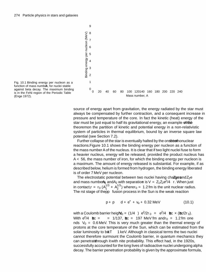
274 Particle physics in stars and galaxies
Fig. 10.1 Binding energy per nucleon as afunction of mass number A, for nuclei stableagainst beta decay. The maximum bindingis in the Fe–Ni region of the Periodic Table(Enge 1972).
Bin
ding
ene
rgy
per
nucl
eon
(MeV
)0
0 20 40 60 80 100 120Mass number, A
140 160 180 200 220 240
1
2
3
4
5
6
7
8
9
source of energy apart from gravitation, the energy radiated by the star mustalways be compensated by further contraction, and a consequent increase inpressure and temperature of the core. In fact the kinetic (heat) energy of thestar must be just equal to half its gravitational energy, an example of the virialtheorem on the partition of kinetic and potential energy in a non-relativisticsystem of particles in thermal equilibrium, bound by an inverse square lawpotential (see Section 7.2).
Further collapse of the star is eventually halted by the onset of thermonuclearreactions. Figure 10.1 shows the binding energy per nucleon as a function ofthe mass number A of the nucleus. It is clear that if two light nuclei fuse to forma heavier nucleus, energy will be released, provided the product nucleus hasA < 56, the mass number of iron, for which the binding energy per nucleon isa maximum. The amount of energy released is substantial. For example, if asdescribed below, helium is formed from hydrogen, the binding energy liberatedis of order 7 MeV per nucleon.
The electrostatic potential between two nuclei having charges Z1e and Z2eand mass numbers A1 and A2 with separation r is V = Z1Z2e2/4πr. When justin contact, r = r0 (A1/3
1 + A1/32 ) where r0 = 1.2 fm is the unit nuclear radius.
The first stage of the p–p fusion process in the Sun is the weak reaction
p + p → d + e+ + ve + 0.32 MeV (10.1)
with a Coulomb barrier height V0 = (1/4π)(e2/2r0
) = (e2/4πhc)×(hc/2r0).
With e2/4πhc = α = 1/137, hc = 197 MeV fm and r0 = 1.2 fm onefinds V0 = 0.6 MeV. This is very much greater than the thermal energy ofprotons at the core temperature of the Sun, which can be estimated from thesolar luminosity to be kT ∼ 1 keV. Although in classical terms the two nucleicannot therefore surmount the Coulomb barrier, in quantum mechanics theycan penetrate through it with finite probability. This effect had, in the 1920s,successfully accounted for the long lives of radioactive nuclei undergoing alphadecay. The barrier penetration probability is given by the approximate formula,
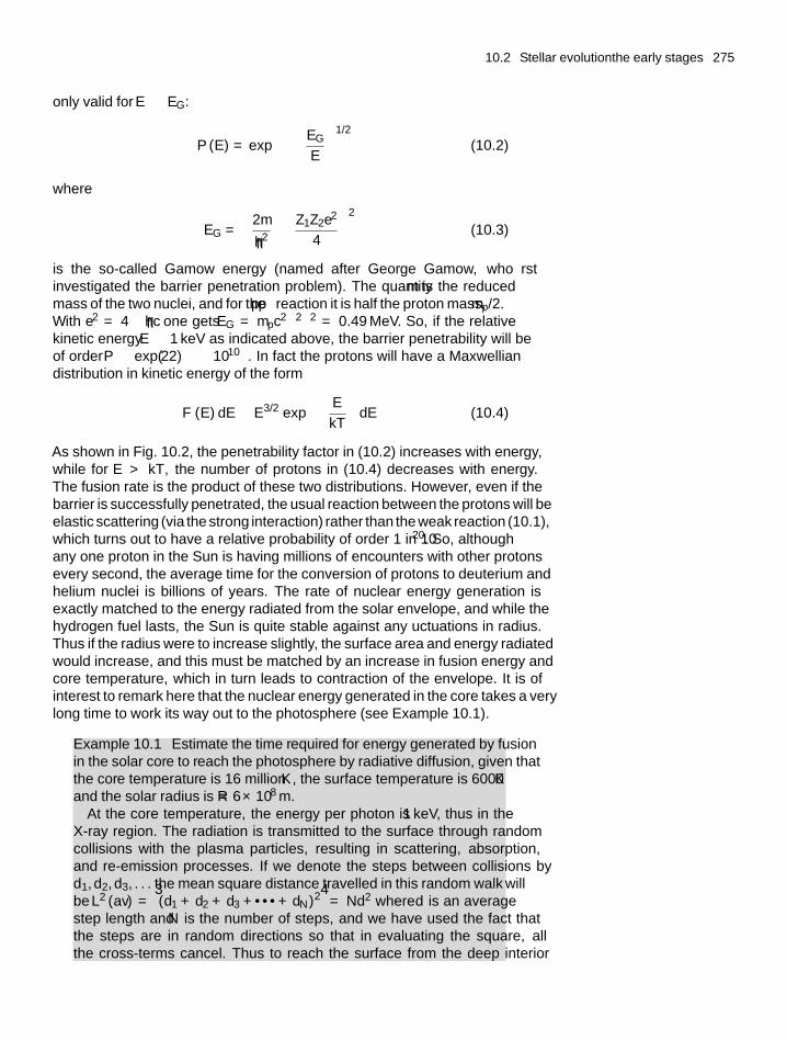
10.2 Stellar evolution—the early stages 275
only valid for E EG:
P (E) = exp
[−(
EG
E
)1/2]
(10.2)
where
EG =(
2m
h2
)(Z1Z2e2
4
)2
(10.3)
is the so-called Gamow energy (named after George Gamow, who firstinvestigated the barrier penetration problem). The quantity m is the reducedmass of the two nuclei, and for the p–p reaction it is half the proton mass, mp/2.With e2 = 4παhc one gets EG = mpc2π2α2 = 0.49 MeV. So, if the relativekinetic energy E ∼ 1 keV as indicated above, the barrier penetrability will beof order P ∼ exp(−22) ∼ 10−10. In fact the protons will have a Maxwelliandistribution in kinetic energy of the form
F (E) dE ∼ E3/2 exp
(− E
kT
)dE (10.4)
As shown in Fig. 10.2, the penetrability factor in (10.2) increases with energy,while for E > kT , the number of protons in (10.4) decreases with energy.The fusion rate is the product of these two distributions. However, even if thebarrier is successfully penetrated, the usual reaction between the protons will beelastic scattering (via the strong interaction) rather than the weak reaction (10.1),which turns out to have a relative probability of order 1 in 1020. So, althoughany one proton in the Sun is having millions of encounters with other protonsevery second, the average time for the conversion of protons to deuterium andhelium nuclei is billions of years. The rate of nuclear energy generation isexactly matched to the energy radiated from the solar envelope, and while thehydrogen fuel lasts, the Sun is quite stable against any fluctuations in radius.Thus if the radius were to increase slightly, the surface area and energy radiatedwould increase, and this must be matched by an increase in fusion energy andcore temperature, which in turn leads to contraction of the envelope. It is ofinterest to remark here that the nuclear energy generated in the core takes a verylong time to work its way out to the photosphere (see Example 10.1).
Example 10.1 Estimate the time required for energy generated by fusionin the solar core to reach the photosphere by radiative diffusion, given thatthe core temperature is 16 million ◦K, the surface temperature is 6000 ◦Kand the solar radius is R = 6 × 10⁸ m.
At the core temperature, the energy per photon is ∼ 1 keV, thus in theX-ray region. The radiation is transmitted to the surface through randomcollisions with the plasma particles, resulting in scattering, absorption,and re-emission processes. If we denote the steps between collisions byd1, d2, d3, . . . the mean square distance travelled in this ‘random walk’ willbe L2 (av) = ⟨(d1 + d2 + d3 + · · · + dN )2⟩ = Nd2 where d is an averagestep length and N is the number of steps, and we have used the fact thatthe steps are in random directions so that in evaluating the square, allthe cross-terms cancel. Thus to reach the surface from the deep interior
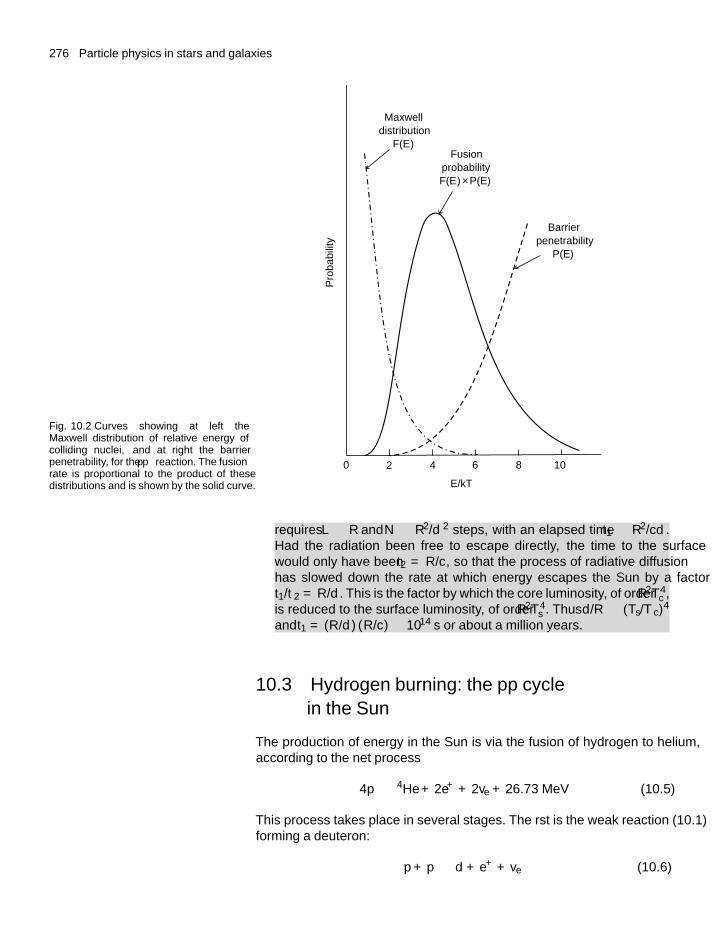
276 Particle physics in stars and galaxies
Fig. 10.2 Curves showing at left theMaxwell distribution of relative energy ofcolliding nuclei, and at right the barrierpenetrability, for the p–p reaction. The fusionrate is proportional to the product of thesedistributions and is shown by the solid curve.
Maxwelldistribution
F(E )Fusion
probabilityF(E ) × P(E )
Barrierpenetrability
P(E )
0 2 4 6 8 10
E/kT
Prob
abili
ty
requires L ∼ R and N ∼ R2/d2 steps, with an elapsed time t1 ∼ R2/cd .Had the radiation been free to escape directly, the time to the surfacewould only have been t2 = R/c, so that the process of radiative diffusionhas slowed down the rate at which energy escapes the Sun by a factort1/t2 = R/d . This is the factor by which the core luminosity, of order R2T 4
c ,is reduced to the surface luminosity, of order R2T 4
s . Thus d/R ∼ (Ts/Tc)4
and t1 = (R/d) (R/c) ∼ 1014 s or about a million years.
10.3 Hydrogen burning: the p–p cyclein the Sun
The production of energy in the Sun is via the fusion of hydrogen to helium,according to the net process
4p → 4He + 2e+ + 2ve + 26.73 MeV (10.5)
This process takes place in several stages. The first is the weak reaction (10.1)forming a deuteron:
p + p → d + e+ + ve (10.6)
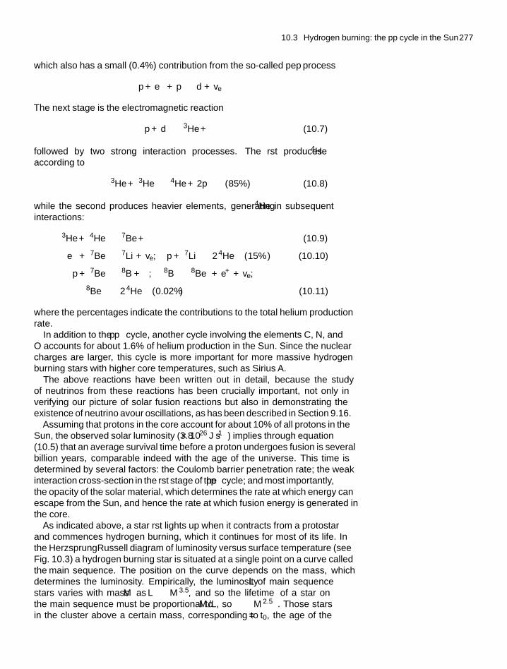
10.3 Hydrogen burning: the p–p cycle in the Sun 277
which also has a small (0.4%) contribution from the so-called ‘pep’ process
p + e− + p → d + ve
The next stage is the electromagnetic reaction
p + d → 3He + γ (10.7)
followed by two strong interaction processes. The first produces 4Heaccording to
3He + 3He → 4He + 2p (85%) (10.8)
while the second produces heavier elements, generating 4He in subsequentinteractions:
3He + 4He → 7Be + γ (10.9)
e− + 7Be → 7Li + ve; p + 7Li → 2 4He (15% ) (10.10)
p + 7Be → 8B + γ; 8B → 8Be∗ + e+ + ve;
8Be∗ → 2 4He (0.02%) (10.11)
where the percentages indicate the contributions to the total helium productionrate.
In addition to the p–p cycle, another cycle involving the elements C, N, andO accounts for about 1.6% of helium production in the Sun. Since the nuclearcharges are larger, this cycle is more important for more massive hydrogenburning stars with higher core temperatures, such as Sirius A.
The above reactions have been written out in detail, because the studyof neutrinos from these reactions has been crucially important, not only inverifying our picture of solar fusion reactions but also in demonstrating theexistence of neutrino flavour oscillations, as has been described in Section 9.16.
Assuming that protons in the core account for about 10% of all protons in theSun, the observed solar luminosity (3.8 × 1026 J s−1) implies through equation(10.5) that an average survival time before a proton undergoes fusion is severalbillion years, comparable indeed with the age of the universe. This time isdetermined by several factors: the Coulomb barrier penetration rate; the weakinteraction cross-section in the first stage of the p–p cycle; and most importantly,the opacity of the solar material, which determines the rate at which energy canescape from the Sun, and hence the rate at which fusion energy is generated inthe core.
As indicated above, a star first lights up when it contracts from a ‘protostar’and commences hydrogen burning, which it continues for most of its life. Inthe Herzsprung–Russell diagram of luminosity versus surface temperature (seeFig. 10.3) a hydrogen burning star is situated at a single point on a curve calledthe main sequence. The position on the curve depends on the mass, whichdetermines the luminosity. Empirically, the luminosity L of main sequencestars varies with mass M as L ∝ M 3.5, and so the lifetime τ of a star onthe main sequence must be proportional to M /L, so τ ∝ M −2.5. Those starsin the cluster above a certain mass, corresponding to τ = t0, the age of the
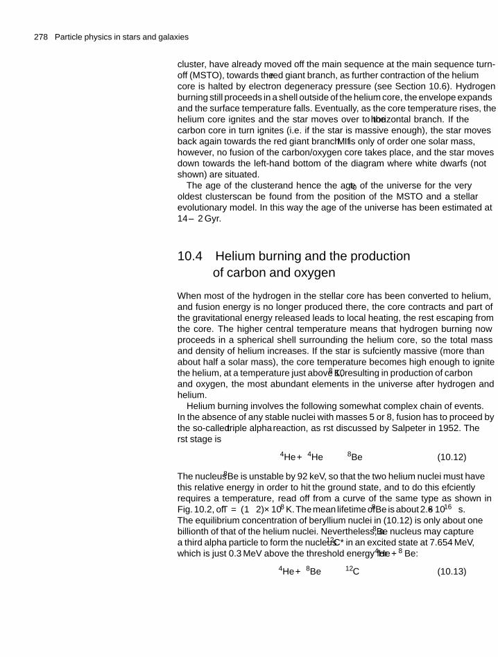
278 Particle physics in stars and galaxies
cluster, have already moved off the main sequence at the main sequence turn-off (MSTO), towards the red giant branch, as further contraction of the heliumcore is halted by electron degeneracy pressure (see Section 10.6). Hydrogenburning still proceeds in a shell outside of the helium core, the envelope expandsand the surface temperature falls. Eventually, as the core temperature rises, thehelium core ignites and the star moves over to the horizontal branch. If thecarbon core in turn ignites (i.e. if the star is massive enough), the star movesback again towards the red giant branch. If M is only of order one solar mass,however, no fusion of the carbon/oxygen core takes place, and the star movesdown towards the left-hand bottom of the diagram where white dwarfs (notshown) are situated.
The age of the cluster—and hence the age t0 of the universe for the veryoldest clusters—can be found from the position of the MSTO and a stellarevolutionary model. In this way the age of the universe has been estimated at14 ± 2 Gyr.
10.4 Helium burning and the productionof carbon and oxygen
When most of the hydrogen in the stellar core has been converted to helium,and fusion energy is no longer produced there, the core contracts and part ofthe gravitational energy released leads to local heating, the rest escaping fromthe core. The higher central temperature means that hydrogen burning nowproceeds in a spherical shell surrounding the helium core, so the total massand density of helium increases. If the star is sufficiently massive (more thanabout half a solar mass), the core temperature becomes high enough to ignitethe helium, at a temperature just above 108 K, resulting in production of carbonand oxygen, the most abundant elements in the universe after hydrogen andhelium.
Helium burning involves the following somewhat complex chain of events.In the absence of any stable nuclei with masses 5 or 8, fusion has to proceed bythe so-called triple alpha reaction, as first discussed by Salpeter in 1952. Thefirst stage is
4He + 4He ←→ 8Be (10.12)
The nucleus 8Be is unstable by 92 keV, so that the two helium nuclei must havethis relative energy in order to ‘hit’ the ground state, and to do this efficientlyrequires a temperature, read off from a curve of the same type as shown inFig. 10.2, of T = (1−2)×108 K.The mean lifetime of 8Be is about 2.6×10⁻¹⁶ s.The equilibrium concentration of beryllium nuclei in (10.12) is only about onebillionth of that of the helium nuclei. Nevertheless, a 8Be nucleus may capturea third alpha particle to form the nucleus 12C* in an excited state at 7.654 MeV,which is just 0.3 MeV above the threshold energy for 4He +8 Be:
4He + 8Be ←→ 12C∗ (10.13)
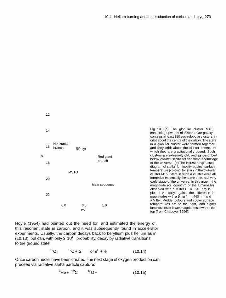
10.4 Helium burning and the production of carbon and oxygen 279
Horizontalbranch
MSTO
Main sequence
Red giantbranch
12
14
16
18
20
22
0.0 0.5 1.0B–V
RR Lyr
V
Fig. 10.3 (a) The globular cluster M13,containing upwards of 105 stars. Our galaxycontains at least 150 such globular clusters, inorbit about the centre of the galaxy. The starsin a globular cluster were formed together,and they orbit about the cluster centre, towhich they are gravitationally bound. Suchclusters are extremely old, and as describedbelow, can be used to set an estimate of the ageof the universe. (b) The Herzsprung–Russelldiagram of stellar luminosity against surfacetemperature (colour), for stars in the globularcluster M15. Stars in such a cluster were allformed at essentially the same time, at a veryearly stage of the universe. In this graph, themagnitude (or logarithm of the luminosity)observed with a V filter (λ = 540 nm) isplotted vertically against the difference inmagnitudes with a B filter (λ = 440 nm) anda V filter. Redder colours and cooler surfacetemperatures are to the right, and higherluminosities or lower magnitudes towards thetop (from Chaboyer 1996).
Hoyle (1954) had pointed out the need for, and estimated the energy of,this resonant state in carbon, and it was subsequently found in acceleratorexperiments. Usually, the carbon decays back to beryllium plus helium as in(10.13), but can, with only 3 × 10⁻⁴ probability, decay by radiative transitionsto the ground state:
12C∗ −→ 12C + 2γ(or e+ + e−) (10.14)
Once carbon nuclei have been created, the next stage of oxygen production canproceed via radiative alpha particle capture:
4He + 12C −→ 16O + γ (10.15)
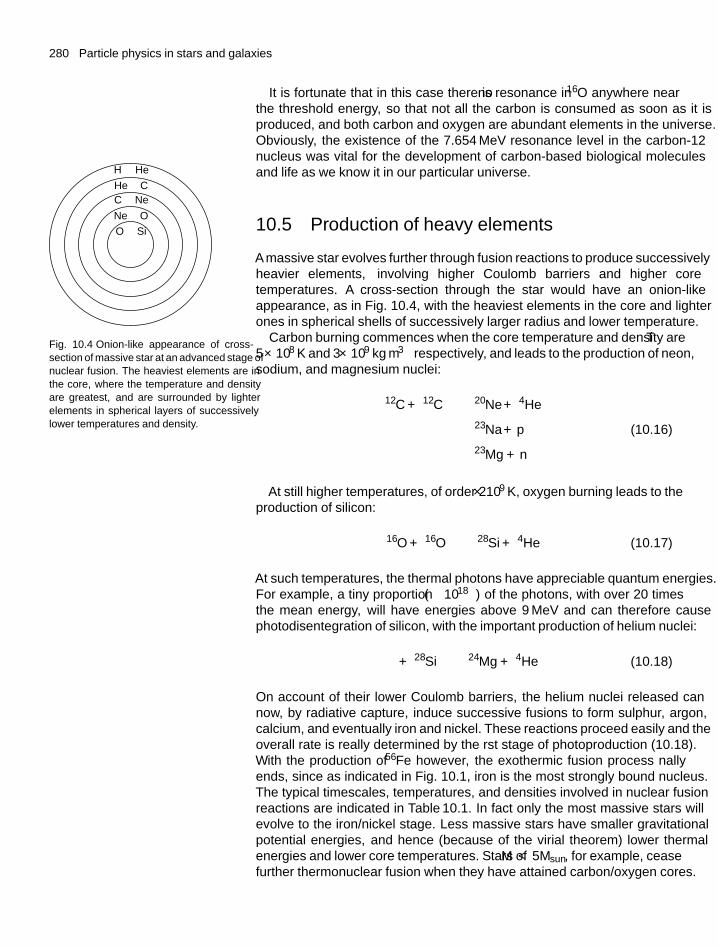
280 Particle physics in stars and galaxies
It is fortunate that in this case there is no resonance in 16O anywhere nearthe threshold energy, so that not all the carbon is consumed as soon as it isproduced, and both carbon and oxygen are abundant elements in the universe.Obviously, the existence of the 7.654 MeV resonance level in the carbon-12nucleus was vital for the development of carbon-based biological moleculesand life as we know it in our particular universe.
10.5 Production of heavy elements
A massive star evolves further through fusion reactions to produce successivelyheavier elements, involving higher Coulomb barriers and higher coretemperatures. A cross-section through the star would have an onion-likeappearance, as in Fig. 10.4, with the heaviest elements in the core and lighterones in spherical shells of successively larger radius and lower temperature.
H → He
He → CC → Ne
Ne → O
O → Si
Fig. 10.4 Onion-like appearance of cross-section of massive star at an advanced stage ofnuclear fusion. The heaviest elements are inthe core, where the temperature and densityare greatest, and are surrounded by lighterelements in spherical layers of successivelylower temperatures and density.
Carbon burning commences when the core temperature and density are T ∼5×10⁸ K and 3×10⁹ kg m−3 respectively, and leads to the production of neon,sodium, and magnesium nuclei:
12C + 12C −→ 20Ne + 4He
−→ 23Na + p (10.16)
−→ 23Mg + n
At still higher temperatures, of order 2 × 10⁹ K, oxygen burning leads to theproduction of silicon:
16O + 16O −→ 28Si + 4He (10.17)
At such temperatures, the thermal photons have appreciable quantum energies.For example, a tiny proportion (∼ 10−18) of the photons, with over 20 timesthe mean energy, will have energies above 9 MeV and can therefore causephotodisentegration of silicon, with the important production of helium nuclei:
γ + 28Si −→ 24Mg + 4He (10.18)
On account of their lower Coulomb barriers, the helium nuclei released cannow, by radiative capture, induce successive fusions to form sulphur, argon,calcium, and eventually iron and nickel. These reactions proceed easily and theoverall rate is really determined by the first stage of photoproduction (10.18).With the production of 56Fe however, the exothermic fusion process finallyends, since as indicated in Fig. 10.1, iron is the most strongly bound nucleus.The typical timescales, temperatures, and densities involved in nuclear fusionreactions are indicated in Table 10.1. In fact only the most massive stars willevolve to the iron/nickel stage. Less massive stars have smaller gravitationalpotential energies, and hence (because of the virial theorem) lower thermalenergies and lower core temperatures. Stars of M < 5Msun, for example, ceasefurther thermonuclear fusion when they have attained carbon/oxygen cores.
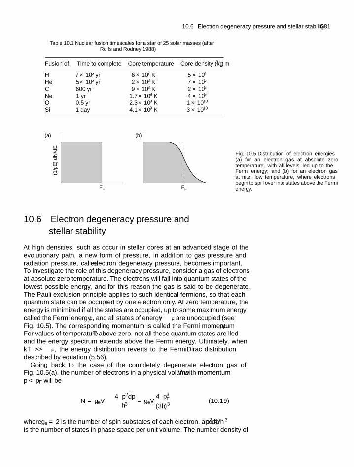
10.6 Electron degeneracy pressure and stellar stability 281
Table 10.1 Nuclear fusion timescales for a star of 25 solar masses (afterRolfs and Rodney 1988)
Fusion of: Time to complete Core temperature Core density (kg m−3)
H 7 × 10⁶ yr 6 × 10⁷ K 5 × 10⁴
He 5 × 10⁵ yr 2 × 10⁸ K 7 × 10⁵
C 600 yr 9 × 10⁸ K 2 × 10⁸
Ne 1 yr 1.7 × 10⁹ K 4 × 10⁹
O 0.5 yr 2.3 × 10⁹ K 1 × 10¹⁰
Si 1 day 4.1 × 10⁹ K 3 × 10¹⁰
EFEF
(a) (b)
(1/p
E)
dN/d
E
Fig. 10.5 Distribution of electron energies(a) for an electron gas at absolute zerotemperature, with all levels filled up to theFermi energy; and (b) for an electron gasat finite, low temperature, where electronsbegin to spill over into states above the Fermienergy.
10.6 Electron degeneracy pressure andstellar stability
At high densities, such as occur in stellar cores at an advanced stage of theevolutionary path, a new form of pressure, in addition to gas pressure andradiation pressure, called electron degeneracy pressure, becomes important.To investigate the role of this degeneracy pressure, consider a gas of electronsat absolute zero temperature. The electrons will fall into quantum states of thelowest possible energy, and for this reason the gas is said to be degenerate.The Pauli exclusion principle applies to such identical fermions, so that eachquantum state can be occupied by one electron only. At zero temperature, theenergy is minimized if all the states are occupied, up to some maximum energycalled the Fermi energy εF, and all states of energy ε > εF are unoccupied (seeFig. 10.5). The corresponding momentum is called the Fermi momentum pF.For values of temperature T above zero, not all these quantum states are filledand the energy spectrum extends above the Fermi energy. Ultimately, whenkT >> εF, the energy distribution reverts to the Fermi–Dirac distributiondescribed by equation (5.56).
Going back to the case of the completely degenerate electron gas ofFig. 10.5(a), the number of electrons in a physical volume V with momentump < pF will be
N = geV∫
4πp2dp
h3= geV
4πp3F
(3h)3(10.19)
where ge = 2 is the number of spin substates of each electron, and 4πp2dp/h3
is the number of states in phase space per unit volume. The number density of
282 Particle physics in stars and galaxies
electrons will be n = N/V so that
pF = h
[3n
(8π)
]1/3
(10.20)
If the electrons are non-relativistic, that is, pF mec, their kinetic energy isp2/2me and the kinetic energy density will be
ENR
V=∫
8πp2(
p2
2me
)dp
h3= 8πp5
F
10meh3(10.21)
Using (5.24b), the degeneracy pressure of the electron gas will therefore be
PNR =(
2
3
)(ENR
V
)= 8πp5
F(15meh3
)=[(
3
8π
)2/3
×(
h2
5me
)]n5/3 (10.22)
However, if the electrons are mainly relativistic, that is, if pF � mec, theelectron energy ε ≈ pc and hence
ER
V=∫
8πp2dp(pc)
h3= 2πp4
Fc
h3(10.23)
The corresponding pressure from (5.24a) becomes
PR =(
1
3
)ER
V=[(
hc
4
)·(
3
8π
)1/3]
n4/3 (10.24)
Note that, in both relativistic and non-relativistic cases, the pressure increaseswith the electron density, but more rapidly in the non-relativistic case. Thisturns out to be crucially important in discussing stability of stars in their finalevolutionary stages.
Let us now consider the effects of the gravitational pressure. The gravitationalenergy of a star or of a stellar core of mass M , radius R, volume V , and anassumed uniform mass density ρ is
Egrav =(
3
5
)GM 2
R
The volume-averaged gravitational pressure is (see Example 10.2 below)
Pgrav = Egrav
3V=(
G
5
)(4π
3
)1/3
M 2/3ρ4/3
=(
G
5
)(4π
3
)1/3
M 2/3(
mPA
Z
)4/3
n4/3 (10.25)
In the second line, the mass density ρ of the material of the stellar corecontaining the degenerate electron gas has been expressed in terms of theelectron number density n, where Z and A are the atomic and mass numbersof the nuclei of the core, respectively , and mP is the nucleon mass, so thatn = (Z/A) ρ/mP.
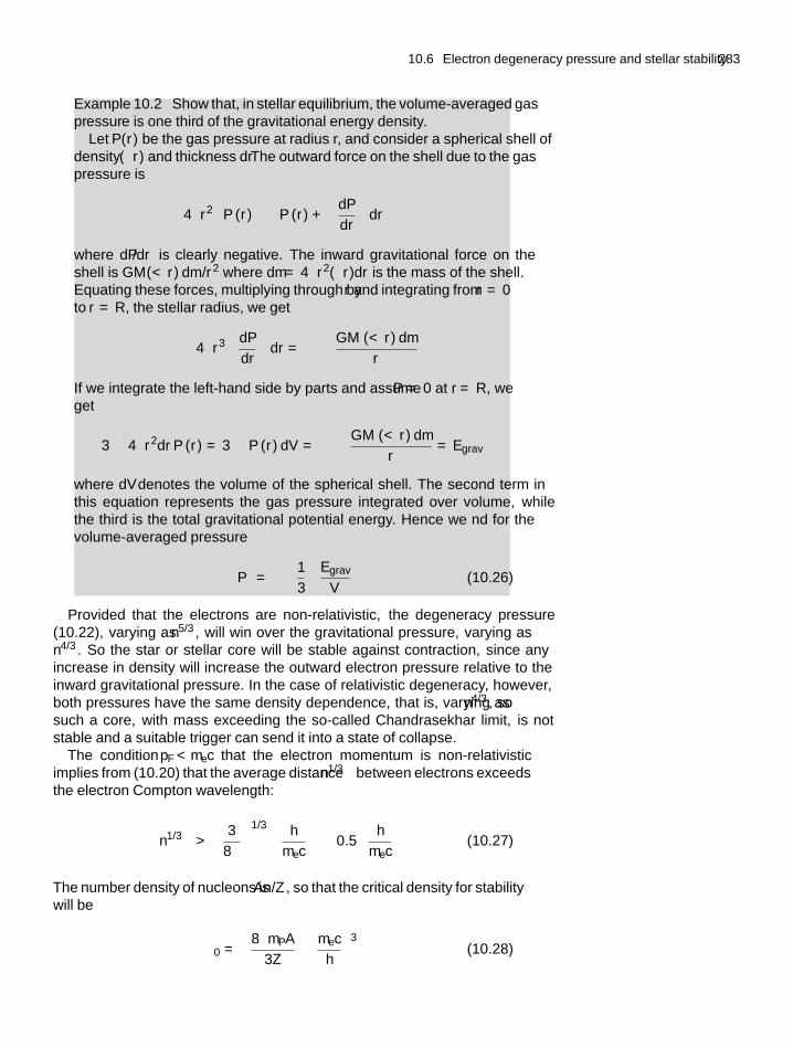
10.6 Electron degeneracy pressure and stellar stability 283
Example 10.2 Show that, in stellar equilibrium, the volume-averaged gaspressure is one third of the gravitational energy density.
Let P(r) be the gas pressure at radius r, and consider a spherical shell ofdensity ρ(r) and thickness dr. The outward force on the shell due to the gaspressure is
4πr2[
P (r) −{
P (r) +(
dP
dr
)dr
}]where dP/dr is clearly negative. The inward gravitational force on theshell is GM (< r) dm/r2 where dm = 4πr2ρ(r)dr is the mass of the shell.Equating these forces, multiplying through by r and integrating from r = 0to r = R, the stellar radius, we get
−∫
4πr3(
dP
dr
)dr = −
∫GM (< r) dm
r
If we integrate the left-hand side by parts and assume P = 0 at r = R, weget
3∫
4πr2dr P (r) = 3∫
P (r) dV = −∫
GM (< r) dm
r= Egrav
where dV denotes the volume of the spherical shell. The second term inthis equation represents the gas pressure integrated over volume, whilethe third is the total gravitational potential energy. Hence we find for thevolume-averaged pressure
〈P〉 = −(
1
3
)Egrav
V(10.26)
Provided that the electrons are non-relativistic, the degeneracy pressure(10.22), varying as n5/3, will win over the gravitational pressure, varying asn4/3. So the star or stellar core will be stable against contraction, since anyincrease in density will increase the outward electron pressure relative to theinward gravitational pressure. In the case of relativistic degeneracy, however,both pressures have the same density dependence, that is, varying as n4/3, sosuch a core, with mass exceeding the so-called Chandrasekhar limit, is notstable and a suitable trigger can send it into a state of collapse.
The condition pF < mec that the electron momentum is non-relativisticimplies from (10.20) that the average distance n−1/3 between electrons exceedsthe electron Compton wavelength:
n−1/3 >
(3
8π
)1/3 ( h
mec
)∼ 0.5
(h
mec
)(10.27)
The number density of nucleons is An/Z , so that the critical density for stabilitywill be
ρ0 =(
8πmPA
3Z
)(mec
h
)3(10.28)
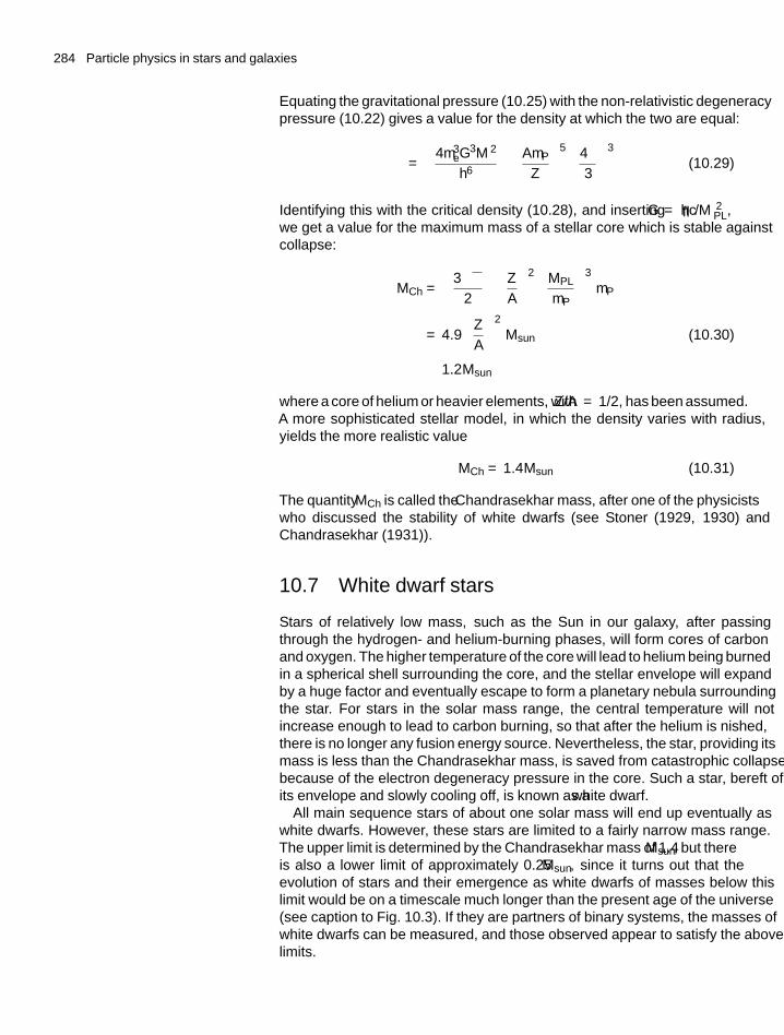
284 Particle physics in stars and galaxies
Equating the gravitational pressure (10.25) with the non-relativistic degeneracypressure (10.22) gives a value for the density at which the two are equal:
ρ =(
4m3eG3M 2
h6
)(AmP
Z
)5 (4π
3
)3
(10.29)
Identifying this with the critical density (10.28), and inserting G = hc/M 2PL,
we get a value for the maximum mass of a stellar core which is stable againstcollapse:
MCh =(
3√
π
2
)(Z
A
)2 (MPL
mP
)3
mP
= 4.9
(Z
A
)2
Msun (10.30)
≈ 1.2 Msun
where a core of helium or heavier elements, with Z/A = 1/2, has been assumed.A more sophisticated stellar model, in which the density varies with radius,yields the more realistic value
MCh = 1.4 Msun (10.31)
The quantity MCh is called the Chandrasekhar mass, after one of the physicistswho discussed the stability of white dwarfs (see Stoner (1929, 1930) andChandrasekhar (1931)).
10.7 White dwarf stars
Stars of relatively low mass, such as the Sun in our galaxy, after passingthrough the hydrogen- and helium-burning phases, will form cores of carbonand oxygen. The higher temperature of the core will lead to helium being burnedin a spherical shell surrounding the core, and the stellar envelope will expandby a huge factor and eventually escape to form a planetary nebula surroundingthe star. For stars in the solar mass range, the central temperature will notincrease enough to lead to carbon burning, so that after the helium is finished,there is no longer any fusion energy source. Nevertheless, the star, providing itsmass is less than the Chandrasekhar mass, is saved from catastrophic collapsebecause of the electron degeneracy pressure in the core. Such a star, bereft ofits envelope and slowly cooling off, is known as a white dwarf.
All main sequence stars of about one solar mass will end up eventually aswhite dwarfs. However, these stars are limited to a fairly narrow mass range.The upper limit is determined by the Chandrasekhar mass of 1.4 Msun, but thereis also a lower limit of approximately 0.25 Msun, since it turns out that theevolution of stars and their emergence as white dwarfs of masses below thislimit would be on a timescale much longer than the present age of the universe(see caption to Fig. 10.3). If they are partners of binary systems, the masses ofwhite dwarfs can be measured, and those observed appear to satisfy the abovelimits.
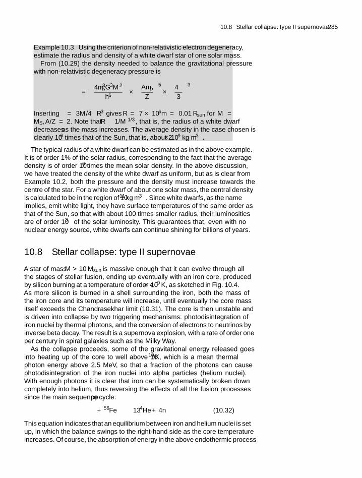
10.8 Stellar collapse: type II supernovae 285
Example 10.3 Using the criterion of non-relativistic electron degeneracy,estimate the radius and density of a white dwarf star of one solar mass.
From (10.29) the density needed to balance the gravitational pressurewith non-relativistic degeneracy pressure is
ρ =(
4m3eG3M 2
h6
)×(
Amp
Z
)5
×(
4π
3
)3
Inserting ρ = 3M /4πR3 gives R = 7 × 10⁶m = 0.01 Rsun for M =MS, A/Z = 2. Note that R ∝ 1/M 1/3, that is, the radius of a white dwarfdecreases as the mass increases. The average density in the case chosen isclearly 106 times that of the Sun, that is, about 2 × 10⁹ kg m−3.
The typical radius of a white dwarf can be estimated as in the above example.It is of order 1% of the solar radius, corresponding to the fact that the averagedensity is of order 106 times the mean solar density. In the above discussion,we have treated the density of the white dwarf as uniform, but as is clear fromExample 10.2, both the pressure and the density must increase towards thecentre of the star. For a white dwarf of about one solar mass, the central densityis calculated to be in the region of 1011 kg m−3. Since white dwarfs, as the nameimplies, emit white light, they have surface temperatures of the same order asthat of the Sun, so that with about 100 times smaller radius, their luminositiesare of order 10−3 of the solar luminosity. This guarantees that, even with nonuclear energy source, white dwarfs can continue shining for billions of years.
10.8 Stellar collapse: type II supernovae
A star of mass M > 10 Msun is massive enough that it can evolve through allthe stages of stellar fusion, ending up eventually with an iron core, producedby silicon burning at a temperature of order 4×10⁹ K, as sketched in Fig. 10.4.As more silicon is burned in a shell surrounding the iron, both the mass ofthe iron core and its temperature will increase, until eventually the core massitself exceeds the Chandrasekhar limit (10.31). The core is then unstable andis driven into collapse by two triggering mechanisms: photodisintegration ofiron nuclei by thermal photons, and the conversion of electrons to neutrinos byinverse beta decay. The result is a supernova explosion, with a rate of order oneper century in spiral galaxies such as the Milky Way.
As the collapse proceeds, some of the gravitational energy released goesinto heating up of the core to well above 1010 K, which is a mean thermalphoton energy above 2.5 MeV, so that a fraction of the photons can causephotodisintegration of the iron nuclei into alpha particles (helium nuclei).With enough photons it is clear that iron can be systematically broken downcompletely into helium, thus reversing the effects of all the fusion processessince the main sequence pp cycle:
γ + 56Fe ←→ 134He + 4n (10.32)
This equation indicates that an equilibrium between iron and helium nuclei is setup, in which the balance swings to the right-hand side as the core temperatureincreases. Of course, the absorption of energy in the above endothermic process
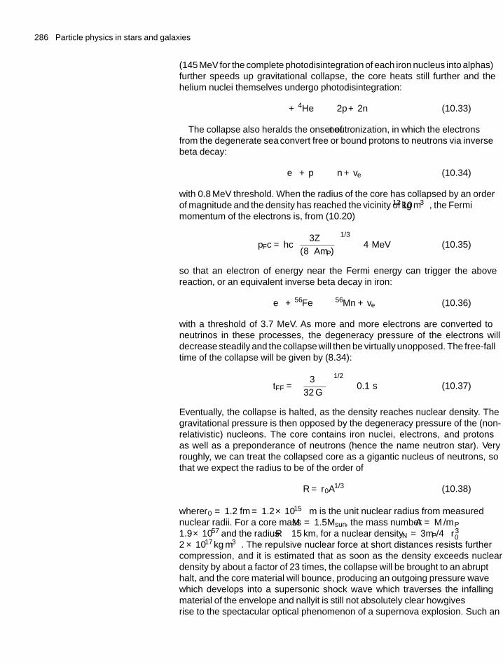
286 Particle physics in stars and galaxies
(145 MeV for the complete photodisintegration of each iron nucleus into alphas)further speeds up gravitational collapse, the core heats still further and thehelium nuclei themselves undergo photodisintegration:
γ + 4He ←→ 2p + 2n (10.33)
The collapse also heralds the onset of neutronization, in which the electronsfrom the degenerate ‘sea’ convert free or bound protons to neutrons via inversebeta decay:
e− + p ←→ n + ve (10.34)
with 0.8 MeV threshold. When the radius of the core has collapsed by an orderof magnitude and the density has reached the vicinity of 1012 kg m−3, the Fermimomentum of the electrons is, from (10.20)
pFc = hc
[3Zρ
(8πAmP)
]1/3
∼ 4 MeV (10.35)
so that an electron of energy near the Fermi energy can trigger the abovereaction, or an equivalent inverse beta decay in iron:
e− + 56Fe ←→ 56Mn + ve (10.36)
with a threshold of 3.7 MeV. As more and more electrons are converted toneutrinos in these processes, the degeneracy pressure of the electrons willdecrease steadily and the collapse will then be virtually unopposed. The free-falltime of the collapse will be given by (8.34):
tFF =(
3π
32 Gρ
)1/2
∼ 0.1 s (10.37)
Eventually, the collapse is halted, as the density reaches nuclear density. Thegravitational pressure is then opposed by the degeneracy pressure of the (non-relativistic) nucleons. The core contains iron nuclei, electrons, and protonsas well as a preponderance of neutrons (hence the name neutron star). Veryroughly, we can treat the collapsed core as a gigantic nucleus of neutrons, sothat we expect the radius to be of the order of
R = r0A1/3 (10.38)
where r0 = 1.2 fm = 1.2 × 10⁻¹⁵ m is the unit nuclear radius from measurednuclear radii. For a core mass M = 1.5 Msun, the mass number A = M /mP ∼1.9 × 1057 and the radius R ∼ 15 km, for a nuclear density ρN = 3mP/4πr3
0 ∼2 × 10¹⁷ kg m−3. The repulsive nuclear force at short distances resists furthercompression, and it is estimated that as soon as the density exceeds nucleardensity by about a factor of 2–3 times, the collapse will be brought to an abrupthalt, and the core material will ‘bounce’, producing an outgoing pressure wavewhich develops into a supersonic shock wave which traverses the infallingmaterial of the envelope and finally—it is still not absolutely clear how—givesrise to the spectacular optical phenomenon of a supernova explosion. Such an
10.8 Stellar collapse: type II supernovae 287
event, resulting from the collapse of a massive star, is known as a Type IIsupernova.
As the initial collapse proceeds, the reactions (10.34) and (10.36) will result inemission of neutrinos. In particular a short, few millisecond burst of 1056−1057
neutrinos νe will accompany the outgoing shock wave. They will have energiesof a few MeVs and account for up to 5% of the total gravitational energyreleased. However, as soon as the core density exceeds about 1015 kg m−3, itbecomes effectively opaque, even to neutrinos, and they become trapped in thecontracting material.
The total gravitational energy released in the collapse to a neutron star of 1.5solar masses and uniform density will be (taking the above values of A and r0):
Egrav =(
3
5
)Gm2
PA5/3
r0
= 3.0 × 1046 J (10.39)
= 1.8 × 1059 MeV
which amounts therefore to about 100 MeV per nucleon. Note that this impliesthat an original uncontracted mass of 1.55 Msun of nucleons will result ina neutron star of mass only 1.4 Msun. This energy release is much largerthan the energy required to disintegrate the iron into its constituent nucleons(the binding energy per nucleon in iron is 8 MeV) or to convert protons andelectrons to neutrons and neutrinos (0.8 MeV per nucleon). The huge amountof energy released, however, remains temporarily locked in the core, whichenters a ‘thermal phase’in which photons, electron–positron pairs and neutrino–antineutrino pairs, together with the neutrons and a few protons and heaviernuclei reach thermal equilibrium. All flavours of neutrino and antineutrino willbe generated in this thermal phase:
γ ←→ e+ + e− ←→ vi + vi (10.40)
where i = e, μ, τ. The mean free path for neutrinos in the core material dependson both charged and neutral current scattering by nucleons, electrons, andnuclei. As an indication we consider the charged current scattering (10.41)of νe by neutrons. The cross-section is of order G2
Fp2f from (1.18) and (1.27),
where pf = E ∼ (Eν −Q) is the neutrino energy above the (negative) threshold(Q = −0.8 MeV)—see Problem 10.7. In detail the cross-section is
σ(ve + n → p + e−) =
(G2
F
π
)[1 + 3g2
A
]E2 = 0.94 × 10−43E2 cm2
(10.41)
where gA = 1.26 is an axial–vector coupling constant and E is in MeV. For atypical nuclear density of ρ = 2 × 10¹⁷ kg m−3, the neutrino mean free pathor diffusion length would be of order λ = 1/σN0ρ ∼ 900/E2 m, which for atypical value of E = 20 MeV, means λ ∼ 2 m only. This process is just one ofneutrino absorption. For neutral current scattering of neutrinos (the only optionfor muon- and tau-neutrinos), the mean free path would be several times bigger,of order 5–10 m.
288 Particle physics in stars and galaxies
In each neutral current scattering process (analogously to the case of photondiffusion through the Sun in Example 10.1 above), the neutrino will emerge inan arbitrary direction, so that after N successive scatters, this ‘random walk’will carry the neutrino a root mean square straight line distance of λN 1/2.Identifying this with the core radius R, we obtain a diffusion time from thecentral region to the surface of t ∼ R2/λc ∼ 0.1 − 1 s. Since neutrinos are theonly particles which are able to escape, the 100 MeVgravitational energy releaseper nucleon is divided among the six flavours of neutrino/antineutrino, anddetailed computer simulations indeed indicate that neutrinos and antineutrinosof all flavours are emitted from the core in comparable numbers over a periodof 0.1–10 s, with average energy ∼ 15 MeV and with an approximately Fermi–Dirac distribution as in (5.56). They are emitted from a so-called neutrinospherewithin a few metres of the surface. Neutrinos account for 99% of the totalgravitational energy released in (10.39). The spectacular optical display of aType II supernova explosion accounts for only 1% of the total energy release.
10.9 Neutrinos from SN 1987A
Figure 10.6 shows a photograph of the supernova SN1987A in the LargeMagellanic Cloud, a mini-galaxy about 60 kpc from the Milky Way. It isfamous because it was the first supernova from which interactions of the emittedneutrinos have been observed, in fact simultaneously in the large Kamiokande(Hirata et al. 1987) and IMB (Bionta et al. 1987) water Cerenkov detectors(with masses of 2 kton and 7 kton respectively) and in the smaller (0.2 kton)Baksan liquid scintillator detector (Alekseev et al. 1987). (All these detectorswere originally designed to search for proton decay.) The neutrino pulse wasactually detected about 7 h before the optical signal became detectable.
The principal reactions that could lead to detection of supernova neutrinosin a water detector are as follows:
ve + p → n + e+ (10.42a)
v + e− → v + e− (10.42b)
v + e− → v + e− (10.42c)
The secondary electrons or positrons from these reactions have relativisticvelocities and part of their energy loss in traversing the water appears in theform of Cerenkov light (see Section 9.6) which is detected by an array ofphotomultipliers, as in Fig. 4.7.
The first reaction (10.42a) has a threshold of Q = 1.8 MeVand a cross-sectionrising as the square of the neutrino energy, as in (1.23), with a value of 10−41 cm2
per proton at Eν = 10 MeV. The angular distribution of the secondary lepton isalmost isotropic. The second and third reactions go via both neutral and chargedcurrent channels for electron-neutrinos/antineutrinos, and via neutral currentsonly for muon and tauon neutrinos/antineutrinos. Although not negligible, thesummed cross-section for these reactions (which vary as Eν) is only 10−43 cm2
per electron at 10 MeV. So, although in water there are five electrons for everyfree proton, the event rate for scattering off electrons is an order of magnitudeless than that for the first reaction. Moreover in (10.42a) all the particles will
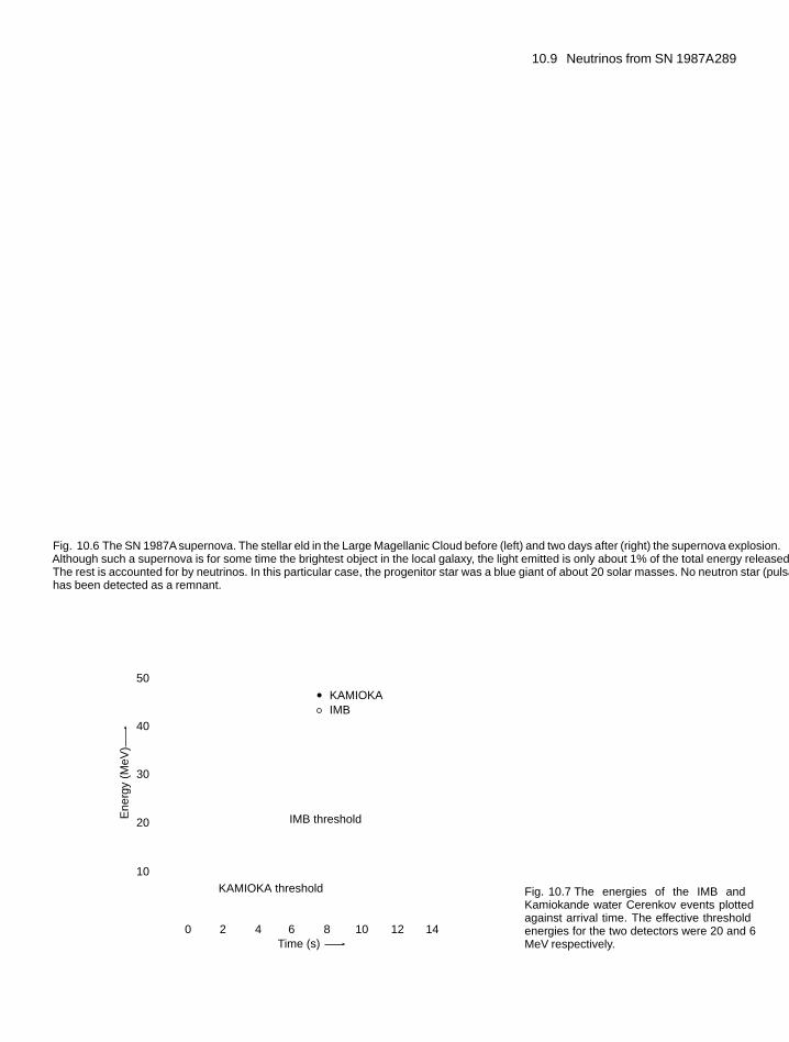
10.9 Neutrinos from SN 1987A 289
Fig. 10.6 The SN 1987A supernova. The stellar field in the Large Magellanic Cloud before (left) and two days after (right) the supernova explosion.Although such a supernova is for some time the brightest object in the local galaxy, the light emitted is only about 1% of the total energy released.The rest is accounted for by neutrinos. In this particular case, the progenitor star was a blue giant of about 20 solar masses. No neutron star (pulsar)has been detected as a remnant.
0
10
20
30
40
50
KAMIOKAIMB
KAMIOKA threshold
IMB thresholdEne
rgy
(MeV
)
2 4 6 8 10 12 14Time (s)
Fig. 10.7 The energies of the IMB andKamiokande water Cerenkov events plottedagainst arrival time. The effective thresholdenergies for the two detectors were 20 and 6MeV respectively.
290 Particle physics in stars and galaxies
have comparable momenta, so that on account of its mass, the proton kineticenergy will be very small and the secondary positron will receive most of theenergy (Ee = Eν −1.8 MeV); while in (10.42b) and (10.42c) the charged leptonreceives typically half the incident energy.
The event rates recorded, together with the known distance to the supernova(60 kpc) could be used to compute the total energy flux in neutrinos andantineutrinos, assuming that the total is six times that for νe alone. Both datasets, when account is taken of detection thresholds, are consistent with a meantemperature of kT ∼ 5 MeV and thus an average neutrino energy at productionof 3.15 kT appropriate to a relativistic Fermi–Dirac distribution. The integratedneutrino luminosity thus calculated from the event rates was
L ≈ 3 × 1046 J
≈ 2 × 1059 MeV (10.43)
with an estimated uncertainty of a factor two, and thus in excellent agreementwith the prediction (10.39).
It perhaps needs to be emphasized that the neutrino flux from a Type IIsupernova is indeed prodigious. Altogether some 1058 neutrinos were emittedfrom SN1987A and even at the Earth, about 170,000 light years distant, theflux was over 1010 neutrinos cm−2.
The recording of neutrinos from SN1987A gave some information onneutrino properties. The fact that they survived a 170,000 year journey withoutattenuation testifies to their stability. Since the neutrino pulse lasted less than10 s, the transit time of neutrinos of different energies was the same within 1part in 5×10¹¹. The time of arrival on the Earth, tE will be given in terms of theemission time from the supernova, tSN, its distance L, and the neutrino mass mand energy E by
tE = tSN +(
L
c
)[1 +(
m2c4
2E2
)]for m2 E2. For two events with different energies E1 and E2 the timedifference will be given by
�t = |�tE − �tSN| =(
Lm2c4
2c
)[1
E21
− 1
E22
](10.44)
If we take as typical values E1 = 10 MeV, E2 = 20 MeV and �t < 10 s, thisequation gives m < 20 eV. A more refined calculation does not result in a betterlimit.
It is of interest to remark here that the neutrino burst may be instrumentalin helping the shock wave to develop the spectacular optical display of asupernova. Early computer models suggested that the outward moving shockmight stall as it met with the infalling matter from outside the core, and produceddisintegration of this material into its constituent nucleons. However, in atleast some of the simulations, when account was taken of the interactions ofthe neutrinos with the envelope material, the transfer of only 1% of the totalneutrino energy was found to be enough to keep the shock wave moving.
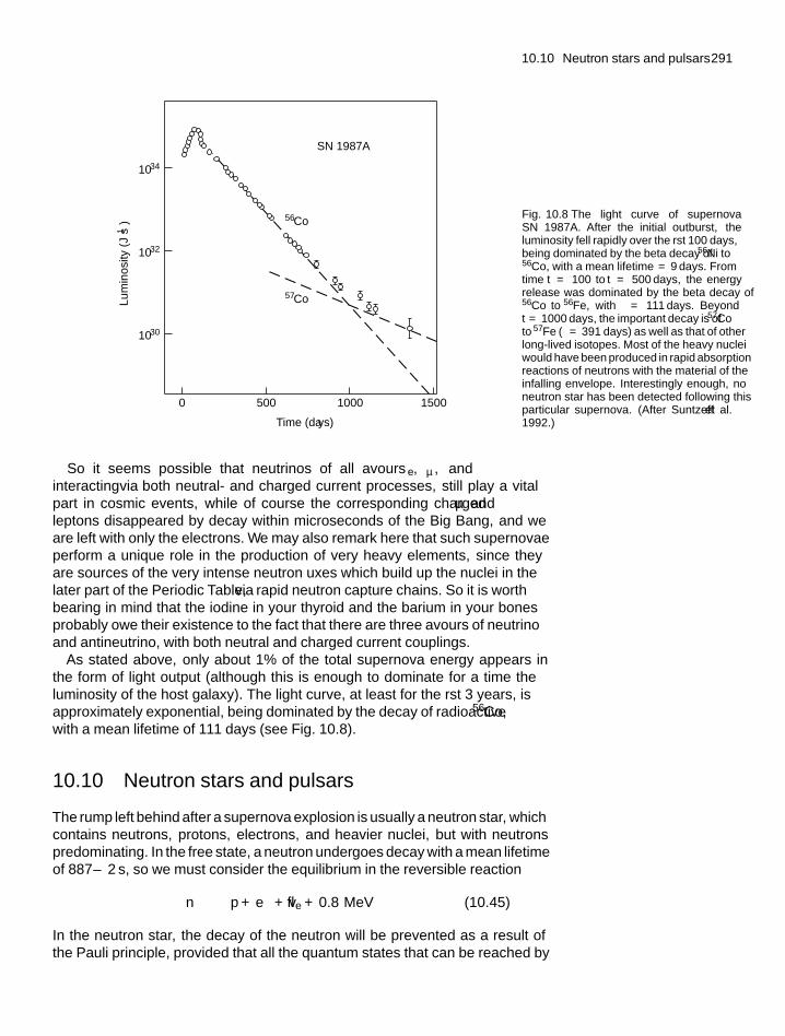
10.10 Neutron stars and pulsars 291
1034
1032
1030
SN 1987A
Time (days)
Lum
inos
ity (
J s–1
)
57Co
56Co
0 500 1000 1500
Fig. 10.8 The light curve of supernovaSN 1987A. After the initial outburst, theluminosity fell rapidly over the first 100 days,being dominated by the beta decay of 56Ni to56Co, with a mean lifetime τ = 9 days. Fromtime t = 100 to t = 500 days, the energyrelease was dominated by the beta decay of56Co to 56Fe, with τ = 111 days. Beyondt = 1000 days, the important decay is of 57Coto 57Fe (τ = 391 days) as well as that of otherlong-lived isotopes. Most of the heavy nucleiwould have been produced in rapid absorptionreactions of neutrons with the material of theinfalling envelope. Interestingly enough, noneutron star has been detected following thisparticular supernova. (After Suntzeff et al.1992.)
So it seems possible that neutrinos of all flavours—νe, νμ, and ντ—interacting via both neutral- and charged current processes, still play a vitalpart in cosmic events, while of course the corresponding charged μ and τ
leptons disappeared by decay within microseconds of the Big Bang, and weare left with only the electrons. We may also remark here that such supernovaeperform a unique role in the production of very heavy elements, since theyare sources of the very intense neutron fluxes which build up the nuclei in thelater part of the Periodic Table, via rapid neutron capture chains. So it is worthbearing in mind that the iodine in your thyroid and the barium in your bonesprobably owe their existence to the fact that there are three flavours of neutrinoand antineutrino, with both neutral and charged current couplings.
As stated above, only about 1% of the total supernova energy appears inthe form of light output (although this is enough to dominate for a time theluminosity of the host galaxy). The light curve, at least for the first 3 years, isapproximately exponential, being dominated by the decay of radioactive 56Co,with a mean lifetime of 111 days (see Fig. 10.8).
10.10 Neutron stars and pulsars
The rump left behind after a supernova explosion is usually a neutron star, whichcontains neutrons, protons, electrons, and heavier nuclei, but with neutronspredominating. In the free state, a neutron undergoes decay with a mean lifetimeof 887 ± 2 s, so we must consider the equilibrium in the reversible reaction
n ←→ p + e− + ve + 0.8 MeV (10.45)
In the neutron star, the decay of the neutron will be prevented as a result ofthe Pauli principle, provided that all the quantum states that can be reached by
292 Particle physics in stars and galaxies
the electron and the proton from the decay are already filled. To a very goodapproximation, if we neglect the Q-value in the decay, this condition is satisfiedwhen the Fermi energies of the degenerate neutrons and electrons are equal,that is, when εF(n) = εF(e), so that the forward and backward reactions are inequilibrium. We know from (10.39) that the neutrons and protons will be non-relativistic, while the electrons will be ultra-relativistic, so that pF(e) pF(n).Then it is clear from (10.20) that the electron number density will be muchsmaller than that of the neutrons, as shown in the numerical Example 10.4.
Example 10.4 Estimate the ratio of numbers of electrons (and protons)to neutrons needed to prevent neutron decay in a neutron star of densityρ = 2 × 10¹⁷ kg m−3.
Assuming that practically all of the nucleons are neutrons, their numberdensity will be nn = 1.2 × 1044 m−3, and their Fermi momentum from(10.20) will be
pF (n) c = hc
[3nn
8π
]1/3
= 300 MeV
while their (non-relativistic) Fermi energy will be
εF (n) = [pF (n) c]2
2Mnc2= 48 MeV
To prevent neutron decay, the Fermi momentum and energy of the(relativistic) electrons therefore need only be of order
pF (e) c = εF (e) = εF (n) = 48 MeV
and the electron number density, proportional to the cube of the Fermimomentum, will be ne = [48/300]3 nn ∼ 0.004 nn. Obviously, np = ne
by charge conservation. So a small proportion, less than 1%, of electronsand protons is sufficient to prevent neutron decay, and the equilibrium in(10.45) is very much to the left.
[Note: Here we have for simplicity neglected the small effect of theprotons. If we include them, the equilibrium condition becomes εF(n) =εF(e)+εF(p). It is left as an exercise to solve the ensuing quadratic equation,and show that the effect of the protons is to reduce the above electronconcentration by 7%].
Although the early theory of neutron stars was developed shortly afterChadwick discovered the neutron in 1932, major experimental interest had toawait the discovery of pulsars by Hewish et al. (1968). Pulsars are rapidlyrotating neutron stars which emit radiation at short and extremely regularintervals, much like a rotating lighthouse beam which crosses the line of sightof an observer with a regular frequency. As indicated below, pulsars possessenormously strong magnetic fields, which are believed to be responsible foracceleration of cosmic ray protons and nuclei. More than 1000 pulsars areknown, with rotational periods ranging from 1.5 ms to 8.5 s. Only about 1%of pulsars can be associated with past supernova remnants, since over millionsof years the neutron stars have drifted away from the remnant nebulae. For afew young pulsars like that in the Crab, the nebula is still associated. This most
10.10 Neutron stars and pulsars 293
famous example of a pulsar has a period of 33 ms, and is the remnant of the ad1054 supernova recorded by the Chinese.
In addition to pulsars like that in the Crab which emit radio waves, about200 X-ray pulsars are known. These are neutron stars which are members ofbinary star systems. Matter accretes from the massive companion star on to themagnetic poles of the neutron star, creating the X-ray emission (‘aurora’). TheX-rays are pulsed with the rotational frequency of the neutron star.
X-ray bursters are associated with neutron stars which have light mainsequence companion stars. Hydrogen is accreted on to the very hot neutronstar surface, and after some time, it reaches a density and temperature leadingto ignition in a thermonuclear explosion lasting several seconds. The processis repeated as more material is accreted. γ-Ray bursters have already beenmentioned in Section 9.11. They are associated with the most violent events inthe universe, releasing an estimated 1046 J in γ-rays, about the same amountof energy as in a Type II supernova explosion. They are possibly produced asa result of neutron star binaries merging to form black holes.
The maximum angular frequency ω of a pulsar will be given by therequirement that the outward centrifugal force on the surface material shouldnot exceed the inward gravitational attraction, that is,
ω2R <GM
R2(10.46)
Inserting the values R ∼ 15 km, M ∼ 1.5 MSun gives for the minimum periodτ = 2π/ω ∼ 1 ms, and indeed no neutron stars are observed with shorterperiods than this. The very high frequencies observed for many pulsars resultbecause much of the angular momentum of the original giant stars is retainedthrough later evolutionary stages and the rotational frequency is enormouslyincreased because of the dramatic contraction to the neutron star size.
The pulsar radiation itself is ascribed to the existence of a rotating magneticdipole inclined at an angle θ to the axis of rotation. For a dipole of strength μ
the electromagnetic power radiated is proportional to the square of the radialacceleration, that is, to ω4:
P ∝ μ ω4 sin2 θ (10.47)
The magnetic field at the surface of a pulsar is of order 108T , this high valueresulting from the trapping and concentration of magnetic flux by the highlyconducting plasma during stellar collapse, the field increasing inversely as thesquare of the radius. The energy lost through the emission of the radiationresults in a small deceleration of the pulsar. If I is the moment of inertia of thepulsar, the rotational energy is 1/2Iω2, so that the rate of change of rotationalenergy or power emitted is
P = Iω
(dω
dt
)∝ ω4
so that
dω
dt= −Aω3
294 Particle physics in stars and galaxies
Observations on the Crab pulsar indicate that at the present time, dω/dt =−2.4 × 10⁻⁹ while ω = 190 s−1. If the initial angular velocity is ωi, the time tfor which it has been spinning to reach the present value of ω is
t =(
1
2A
)[1
ω2− 1
ω2i
]<
1(2Aω2
) = 1
2
ω
(dω/dt)= 1255 yr.
in agreement with its origin in ad 1054.
10.11 Black holes
Neutrons play a similar role in supporting a neutron star as degenerate electronsdo in supporting a white dwarf. The limit to which the degenerate neutron gascan do this is analogous to the Chandrasekhar limit for electron degeneracyin white dwarfs. If we forget about the strong nuclear interactions and generalrelativity effects in high gravitational fields, we can apply (10.29) with thesubstitution A/Z = 1, so that the limit (10.30) therefore becomes
Mmax ∼ 4.9 Msun (10.48)
For neutron stars with masses M > Mmax, the degenerate neutron gasbecomes relativistic, and gravitational collapse is inevitable. However, stronginteractions between the neutrons will tend to make the neutron star mattermore incompressible and increase the maximum mass. On the other hand, thegravitational binding energy of a neutron star is comparable with its mass energy(see (10.39)), so that non-linear gravitational effects associated with the massenergy of the field itself should be included and this will tend to decrease themaximum mass of the neutron star. So (10.48) should only be taken as anindication that the critical mass of neutron stars is a few solar masses.
The fate of a neutron star which undergoes gravitational collapse is a blackhole. Not all black holes are formed in this way. For example, the giant low-metallicity Wolf–Rayet stars are believed to collapse to black holes at the end ofthe carbon burning phase. The crucial property associated with a black hole isthe Schwarzschild radius (2.23) for an object of mass M , given by the formula
rs = 2GM
c2(10.49)
This result was derived by Schwarzschild, who obtained an exact solutionto Einstein’s field equations of general relativity, for the specific case of agravitational field due to a large static mass M . As explained in Chapter 2, ithappens that it can also be found using special relativity and the equivalenceprinciple, or by equating the radial escape velocity from a point mass M to thevelocity of light. As an example of (10.49), the Schwarzschild radius of a starof mass M = 5Msun is rs = 15 km. Equation (10.49) implies that when thephysical radius of a collapsed star falls inside the Schwarzschild radius, thereare no light paths (geodesics) to the outside world. Photons from the star cannotescape its gravitational field and the star becomes black to an outside observer.
To understand how can this be, let us apply the special theory of relativity bycomparing a time interval dt on a stationary clock in a remote inertial frame with
10.12 Hawking radiation from black holes 295
that, dt′, on an identical clock stationary in an inertial frame which has velocityv relative to the first frame, and is instantaneously co-moving with the surfaceof the collapsing star. Then dt′2 = dt2
(1 − v2/c2
). Thus as v → c, dt′ → 0 and
to an observer in the remote frame, the star appears ‘frozen’ in time. Equally,the wavelength of light from a star collapsing inside its Schwarzschild radius
undergoes a redshift according to the relation λ′ = λ/(1 − (v2/c2
))1/2, and the
redshift tends to infinity as v → c. Since the quantum energy of the radiationhv = hc/λ → 0 as λ → ∞, the energy emitted from the star also tends tozero. These phenomena are what would be recorded by an external observer.An observer within the Schwarzschild radius would, however, record lots ofactivity, but would not be able to communicate with the outside world.
Black holes are inevitable consequences of Einstein’s general theory ofrelativity—even if Einstein could not bring himself to believe in their existence.From the general theory it follows that everything possessing energy andmomentum, including photons, will be deflected by a gravitational field andwill be ‘turned around’ if the field is strong enough. The experimental evidencefor the existence of black holes is quite convincing. It rests, for example, onobservation of binary systems in which the motion of the visible star impliesthe existence of a compact invisible companion with mass M > Mmax. Suchsystems are observed as compact X-ray sources, the X-rays being produced asmass from the visible star flows into the black hole. The first candidate for ablack hole was the X-ray source Cygnus X-1, with M = 3.4 Msun. Anothercandidate was V404 Cygni, which included a compact object of M > 6 Msun.Recent investigations show that intense amounts of X-rays are emitted from thecentres of nearly all galaxies. The conclusion is that the X-rays are emitted byvery hot gas flowing into a massive central black hole, typically with a mass of106 − 108 solar masses. For example, the Milky Way possesses a black hole atits centre of 3 × 10⁶ solar masses, identified with the X-ray source SagittariusA∗ (see Problem 10.7).
It is generally considered that some of the most violent events in the universe,such as γ-ray bursts (see Section 9.11) originate from the very small proportion(∼ 1%) of galactic nuclei which are ‘active’—the so-called AGNs. These areassociated with massive black holes at the centres of galaxies which are still veryactive in absorbing large amounts of nearby material—stars, gas, and dust—asdistinct from most galactic nuclei, with black holes which have gone throughthat stage and are now relatively passive. Recently, as mentioned in Chapter 9,it has been found that charged cosmic ray primaries with energies exceeding6 × 1019 eV are correlated in direction with AGNs, presumably because theyare accelerated in the neighbourhood of black holes.
At the other extreme, primordial ‘mini black holes’ might have been createdin the early universe, but if so equation (10.51) below suggests that they wouldhave evaporated long ago if their masses were much below 1012 kg.
10.12 Hawking radiation from black holes
When quantum fluctuations are brought into the picture, it turns out that in thevery strong gravitational fields around them, black holes are actually able to emit(thermal) radiation, as proved by Hawking in 1974. The Hawking temperature
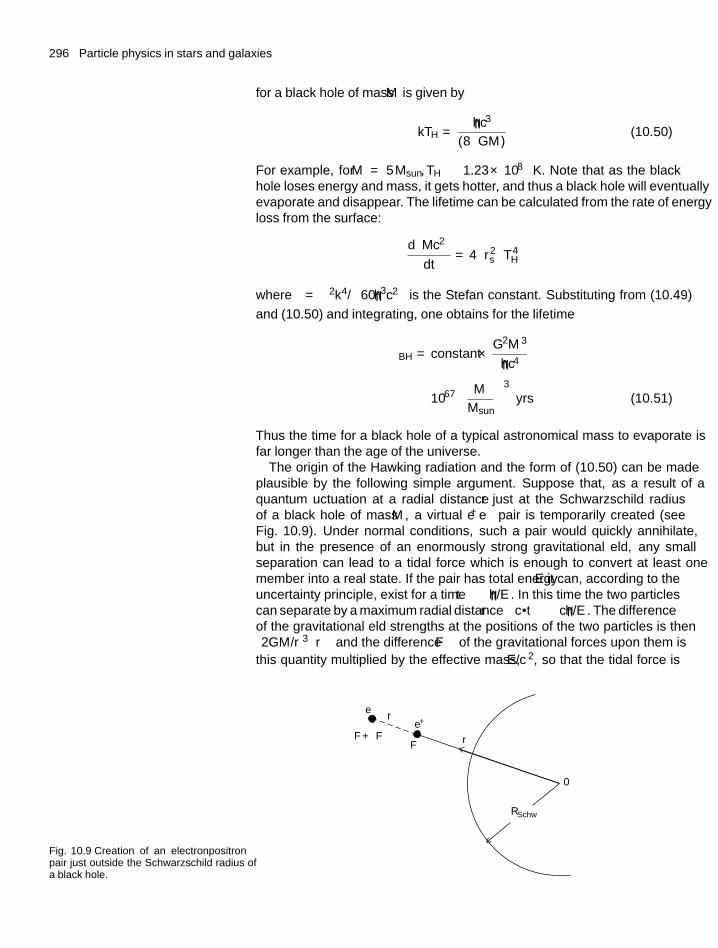
296 Particle physics in stars and galaxies
for a black hole of mass M is given by
kTH = hc3
(8πGM )(10.50)
For example, for M = 5 Msun, TH ∼ 1.23 × 10⁻⁸ K. Note that as the blackhole loses energy and mass, it gets hotter, and thus a black hole will eventuallyevaporate and disappear. The lifetime can be calculated from the rate of energyloss from the surface:
d(Mc2)
dt= 4πr2
s σT 4H
where σ = π2k4/(
60h3c2)
is the Stefan constant. Substituting from (10.49)
and (10.50) and integrating, one obtains for the lifetime
τBH = constant × G2M 3(hc4)
∼ 1067(
M
Msun
)3
yrs (10.51)
Thus the time for a black hole of a typical astronomical mass to evaporate isfar longer than the age of the universe.
The origin of the Hawking radiation and the form of (10.50) can be madeplausible by the following simple argument. Suppose that, as a result of aquantum fluctuation at a radial distance r just at the Schwarzschild radiusof a black hole of mass M , a virtual e+e− pair is temporarily created (seeFig. 10.9). Under normal conditions, such a pair would quickly annihilate,but in the presence of an enormously strong gravitational field, any smallseparation can lead to a tidal force which is enough to convert at least onemember into a real state. If the pair has total energy E it can, according to theuncertainty principle, exist for a time �t ∼ h/E. In this time the two particlescan separate by a maximum radial distance �r ∼ c ·�t ∼ ch/E. The differenceof the gravitational field strengths at the positions of the two particles is then(2GM /r3
)�r and the difference �F of the gravitational forces upon them is
this quantity multiplied by the effective mass, E/c2, so that the tidal force is
Fig. 10.9 Creation of an electron–positronpair just outside the Schwarzschild radius ofa black hole.
Δre–
e+
F +ΔF rF
RSchw
0
10.13 Summary 297
�F ∼ (GM /r3)
h/c. For the gravitational field to be able to create the pair, one
requires �F�r > E, that is, E < h(GM /r3
)1/2. The largest value of E will
be for the minimum value of r, namely r ∼ rs, giving the order-of-magnitudecondition
E ∼ hc3
GM
agreeing with (10.50) up to numerical constants. In the presence of the stronggravitational field, the pair can be separated fast enough that one of them getswell outside of the Schwarzschild radius and escapes as a real particle, whilethe other is sucked back into the black hole.
10.13 Summary
• Stars form from protostars consisting of vast clouds of hydrogenin gravitational collapse, which contract until the core temperaturereaches kT ∼ 1 keV, when thermonuclear fusion of hydrogen to heliumcommences and the star attains hydrostatic equilibrium. This hydrogenfusion on the main sequence of the Herzsprung–Russell diagramcontinues typically for billions of years.
• When the hydrogen fuel is exhausted, fusion of helium to carbon andoxygen takes place, at a higher core temperature and on a much shortertimescale. The star becomes a red giant with a bloated envelope.
• If the stellar mass is of the order of a solar mass or less, the consumptionof helium marks the end of the fusion cycle and of nuclear energyrelease, and the star cools off slowly as a white dwarf with a degenerateelectron core.
• In more massive stars, the core temperature becomes high enoughfor fusion to continue, with production of heavier elements up to nickeland iron.
• If the mass of the iron core exceeds the Chandrasekhar mass of 1.4 solarmasses, it is inherently unstable and suffers catastrophic collapse withformation of a very compact neutron star of nuclear density. About 10%of the mass energy of the star is emitted in the form of a burst of neutrinos,and as a shock wave which gives rise to the optical display of a Type IIsupernova.
• If the core mass is much larger, around 4 to 6 solar masses, the neutronstar is unstable and undergoes further collapse to a black hole. Binarysystems with a black hole as one partner are compact and very intensesources of X-rays, emitted as matter flows into the black hole from thecompanion.
• Black holes can decay by emission of Hawking radiation, which is amanifestation of quantum fluctuations near the Schwarzschild radius of ablack hole. Intense sources of X-rays from the centres of many galaxiesare attributed to emission from very hot gas flowing into massive (108
solar mass) black holes at the galactic centre. Such black holes may beidentified with active galactic nuclei, associated with intense γ-ray burstsas described in Chapter 9.
298 Particle physics in stars and galaxies
Problems
More challenging problems are marked with an asterisk.
(10.1) Estimate the maximum rotational frequency of a whitedwarf star, assuming that it has a mass equal to a solarmass and radius of 1% of the solar radius.
(10.2) Calculate the luminosity (in watts) of the Sun, giventhat its surface temperature is 5780 K and its radius is7×108 m. Solar energy is provided by fusion of heliumfrom hydrogen. If 5% of the hydrogen in the Sun hasso far been converted to helium, estimate the age of theSun, assuming the luminosity to have been constant.
*(10.3) Find the maximum mass for a body containing normalatomic matter (density 104 kg m−3) which doesnot require electron degeneracy pressure in order tomaintain its stability against gravitational collapse.What object might such a body represent?
(10.4) The slow-down of the Crab Pulsar is assumed tobe due to emission of dipole radiation as a resultof its rotating magnetic field as indicated in (10.47).However, one could also ask if the slow-down could bedue to gravitational quadrupole radiation, varying withrotational frequency as ω6 as in (9.28). Show that theobserved values of ω = 190 s−1 and dω/dt = −2.4 ×10⁻⁹ would then be inconsistent with its known age.
*(10.5) Calculate the mass of a black hole with a Schwarzschildradius equal to the particle horizon distance for auniverse of age t0. If the universe had a density equal tothe critical density, at what value of t0 would the massof the universe be equal to that of the black hole?
(10.6) Estimate the radius and mass of a black hole with alifetime equal to that of the universe.
(10.7) Show that, in the reaction ve + p → e+ + n, the cross-section is of order G2
Fp2f where the CMS momentum in
the final state pf ≈ Eν − Q. Here Eν is the antineutrinoenergy, assumed to be small compared with the nucleonrest-mass but large compared with the electron rest-mass, which can be neglected, and Q is the thresholdenergy for the reaction.
*(10.8) A star has been observed (in the infrared) in orbit abouta massive unseen object (black hole) at the centre ofour galaxy, identified with the compact radio and X-ray source Sagittarius A* (see Physics Today, February2003 for reference). The elliptic orbit has a period of 15years and eccentricity of 0.87, and the closest distanceof approach (perigee) is estimated to be 17 light hours.If necessary referring to a text on celestial mechanics,calculate the mass of the black hole and the orbitalvelocity of the star at perigee.
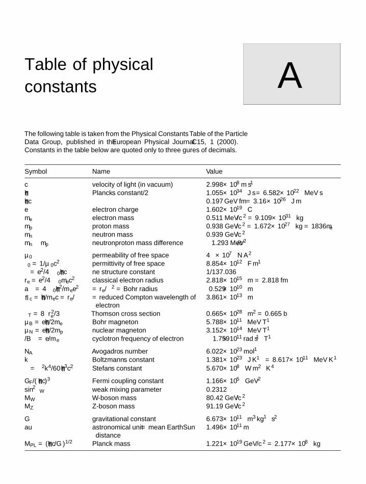
Table of physicalconstants AThe following table is taken from the ‘Physical Constants’Table of the ParticleData Group, published in the European Physical Journal C15, 1 (2000).Constants in the table below are quoted only to three figures of decimals.
Symbol Name Value
c velocity of light (in vacuum) 2.998 × 10⁸ m s−1
h Planck’s constant/2π 1.055 × 10⁻³⁴ J s = 6.582 × 10⁻²² MeV shc 0.197 GeV fm = 3.16 × 10⁻²⁶ J me electron charge 1.602 × 10⁻¹⁹ Cme electron mass 0.511 MeV/c2 = 9.109 × 10⁻³¹ kgmp proton mass 0.938 GeV/c2 = 1.672 × 10⁻²⁷ kg = 1836me
mn neutron mass 0.939 GeV/c2
mn − mp neutron–proton mass difference 1.293 MeV/c2
μ0 permeability of free space 4π × 10−7 N A−2
ε0 = 1/μ0c2 permittivity of free space 8.854 × 10⁻¹² F m−1
α = e2/4πε0hc fine structure constant 1/137.036re = e2/4πε0mec2 classical electron radius 2.818 × 10⁻¹⁵ m = 2.818 fma∞ = 4πε0h2/mee2 = re/α
2 = Bohr radius 0.529 × 10⁻¹⁰ mλc = h/mec = re/α = reduced Compton wavelength of
electron3.861 × 10−13 m
σT = 8πr2e /3 Thomson cross section 0.665 × 10⁻²⁸ m2 = 0.665 b
μB = eh/2me Bohr magneton 5.788 × 10⁻¹¹ MeV T−1
μN = eh/2mp nuclear magneton 3.152 × 10⁻¹⁴ MeV T−1
ω/B = e/me cyclotron frequency of electron 1.759 × 10¹¹ rad s−1 T−1
NA Avogadro’s number 6.022 × 10²³ mol−1
k Boltzmann’s constant 1.381 × 10⁻²³ J K−1 = 8.617 × 10⁻¹¹ MeV K−1
σ = π2k4/60h3c2 Stefan’s constant 5.670 × 10⁻⁸ W m−2 K−4
GF/(hc)3 Fermi coupling constant 1.166 × 10⁻⁵ GeV−2
sin2 θW weak mixing parameter 0.2312MW W-boson mass 80.42 GeV/c2
MZ Z-boson mass 91.19 GeV/c2
G gravitational constant 6.673 × 10⁻¹¹ m3 kg−1 s−2
au astronomical unit = mean Earth–Sundistance
1.496 × 10¹¹ m
MPL = (hc/G)1/2 Planck mass 1.221 × 10¹⁹ GeV/c2 = 2.177 × 10⁻⁸ kg
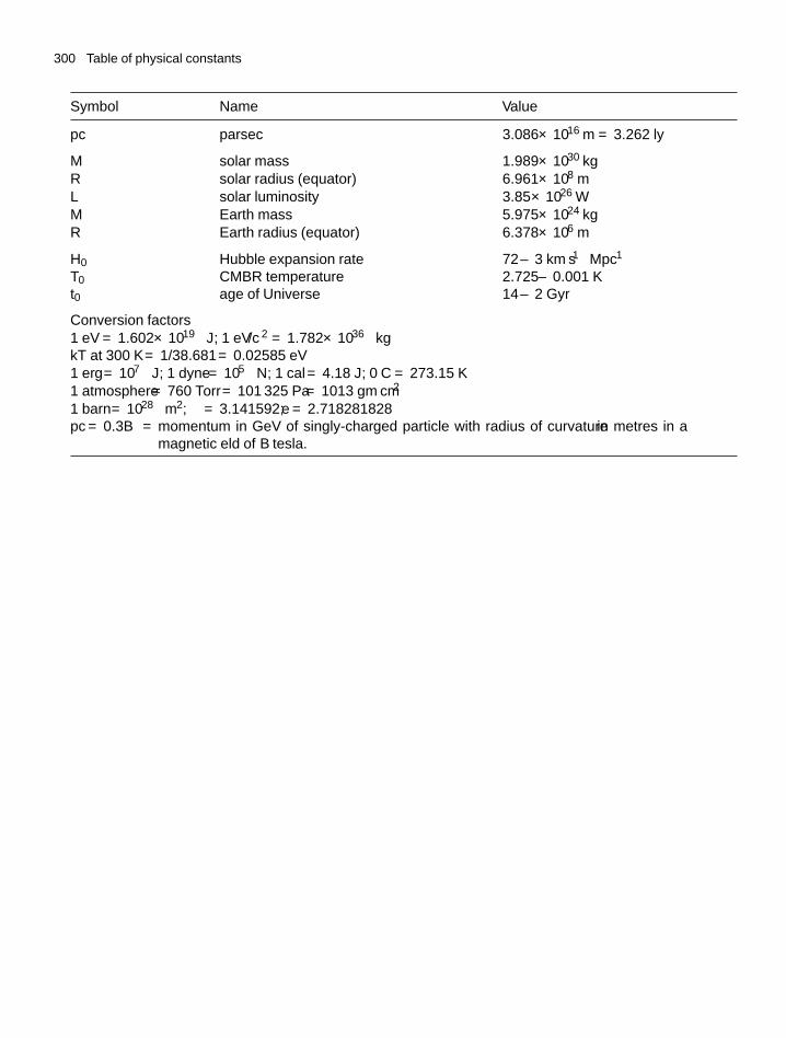
300 Table of physical constants
Symbol Name Value
pc parsec 3.086 × 10¹⁶ m = 3.262 ly
M� solar mass 1.989 × 1030 kgR� solar radius (equator) 6.961 × 10⁸ mL� solar luminosity 3.85 × 1026 WM⊕ Earth mass 5.975 × 1024 kgR⊕ Earth radius (equator) 6.378 × 10⁶ m
H0 Hubble expansion rate 72 ± 3 km s−1 Mpc−1
T0 CMBR temperature 2.725 ± 0.001 Kt0 age of Universe 14 ± 2 Gyr
Conversion factors1 eV = 1.602 × 10⁻¹⁹ J; 1 eV/c2 = 1.782 × 10−36 kgkT at 300 K = 1/38.681 = 0.02585 eV1 erg = 10−7 J; 1 dyne = 10−5 N; 1 cal = 4.18 J; 0 ◦C = 273.15 K1 atmosphere = 760 Torr = 101 325 Pa = 1013 gm cm−2
1 barn = 10−28 m2; π = 3.141592; e = 2.718281828pc = 0.3Bρ = momentum in GeV of singly-charged particle with radius of curvature ρ in metres in a
magnetic field of B tesla.
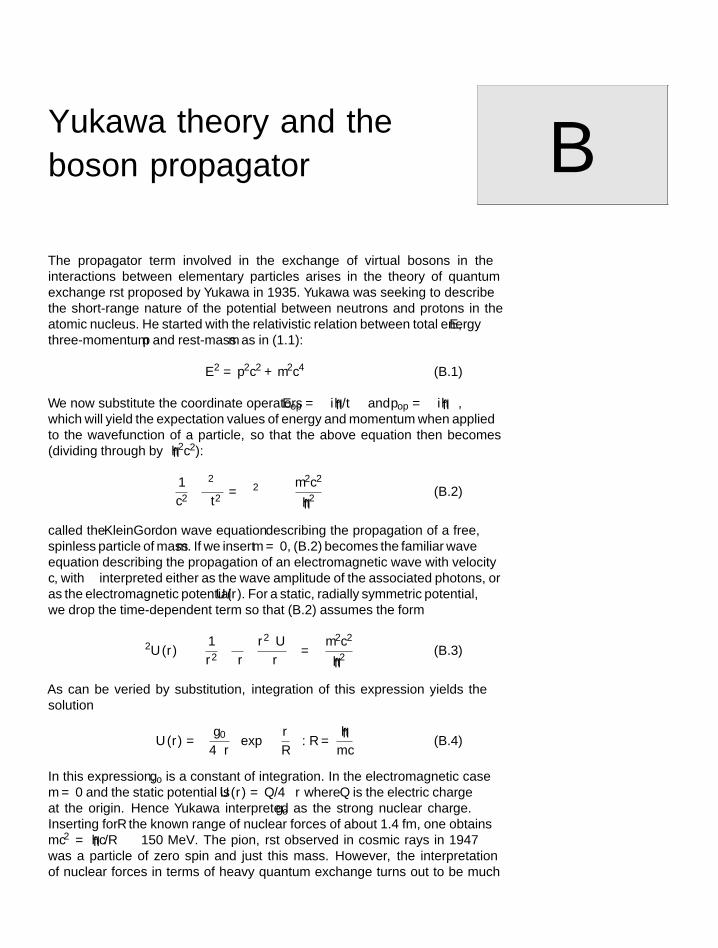
Yukawa theory and theboson propagator BThe propagator term involved in the exchange of virtual bosons in theinteractions between elementary particles arises in the theory of quantumexchange first proposed by Yukawa in 1935. Yukawa was seeking to describethe short-range nature of the potential between neutrons and protons in theatomic nucleus. He started with the relativistic relation between total energy E,three-momentum p and rest-mass m as in (1.1):
E2 = p2c2 + m2c4 (B.1)
We now substitute the coordinate operators Eop = −ih∂/∂t and pop = −ih∇,which will yield the expectation values of energy and momentum when appliedto the wavefunction of a particle, so that the above equation then becomes(dividing through by −h2c2):(
1
c2
)∂2ψ
∂t2= ∇2ψ −
(m2c2
h2
)ψ (B.2)
called the Klein–Gordon wave equation describing the propagation of a free,spinless particle of mass m. If we insert m = 0, (B.2) becomes the familiar waveequation describing the propagation of an electromagnetic wave with velocityc, with ψ interpreted either as the wave amplitude of the associated photons, oras the electromagnetic potential U (r). For a static, radially symmetric potential,we drop the time-dependent term so that (B.2) assumes the form
∇2U (r) ≡(
1
r2
)∂
∂r
(r2∂U
∂r
)=(
m2c2
h2
)ψ (B.3)
As can be verified by substitution, integration of this expression yields thesolution
U (r) =( g0
4πr
)exp(− r
R
): R = h
mc(B.4)
In this expression, go is a constant of integration. In the electromagnetic casem = 0 and the static potential is U (r) = Q/4πr where Q is the electric chargeat the origin. Hence Yukawa interpreted go as the ‘strong nuclear charge’.Inserting for R the known range of nuclear forces of about 1.4 fm, one obtainsmc2 = hc/R ∼ 150 MeV. The pion, first observed in cosmic rays in 1947was a particle of zero spin and just this mass. However, the interpretationof nuclear forces in terms of heavy quantum exchange turns out to be much
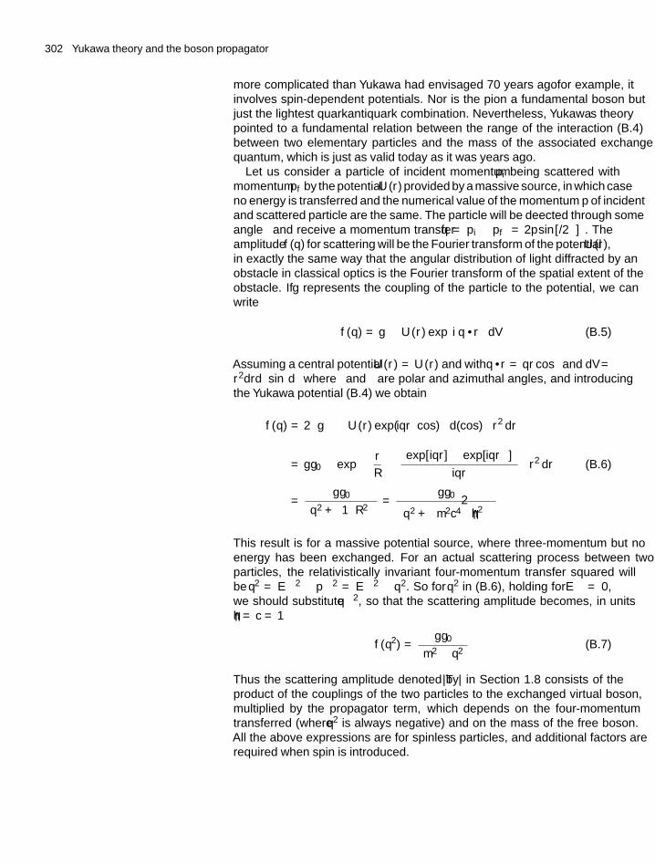
302 Yukawa theory and the boson propagator
more complicated than Yukawa had envisaged 70 years ago—for example, itinvolves spin-dependent potentials. Nor is the pion a fundamental boson butjust the lightest quark–antiquark combination. Nevertheless, Yukawa’s theorypointed to a fundamental relation between the range of the interaction (B.4)between two elementary particles and the mass of the associated exchangequantum, which is just as valid today as it was years ago.
Let us consider a particle of incident momentum pi being scattered withmomentum pf by the potential U (r) provided by a massive source, in which caseno energy is transferred and the numerical value of the momentum p of incidentand scattered particle are the same. The particle will be deflected through someangle θ and receive a momentum transfer q = pi − pf
(= 2p sin [θ/2]). The
amplitude f (q) for scattering will be the Fourier transform of the potential U (r),in exactly the same way that the angular distribution of light diffracted by anobstacle in classical optics is the Fourier transform of the spatial extent of theobstacle. If g represents the coupling of the particle to the potential, we canwrite
f (q) = g∫
U (r) exp(i q · r
)dV (B.5)
Assuming a central potential U (r) = U (r) and with q · r = qr cos θ and dV =r2drdφsinθdθ where θ and φ are polar and azimuthal angles, and introducingthe Yukawa potential (B.4) we obtain
f (q) = 2πg∫∫
U (r) exp(iqr cos θ) d(cos θ) r2 dr
= gg0
∫exp(− r
R
){(exp [iqr] − exp[−iqr])iqr
}r2 dr (B.6)
= gg0(q2 + (1/R2
)) = gg0(q2 +
(m2c4
/h2))
This result is for a massive potential source, where three-momentum but noenergy has been exchanged. For an actual scattering process between twoparticles, the relativistically invariant four-momentum transfer squared willbe q2 = �E2 − �p2 = �E2 − q2. So for q2 in (B.6), holding for �E = 0,we should substitute −q2, so that the scattering amplitude becomes, in unitsh = c = 1
f (q2) = gg0[m2 − q2
] (B.7)
Thus the scattering amplitude denoted by |Tfi| in Section 1.8 consists of theproduct of the couplings of the two particles to the exchanged virtual boson,multiplied by the propagator term, which depends on the four-momentumtransferred (where q2 is always negative) and on the mass of the free boson.All the above expressions are for spinless particles, and additional factors arerequired when spin is introduced.
Perturbative growthof structure in theearly universe
CWe start with the FLRW model described in Chapters 2 and 5, which assumesa completely isotropic and homogeneous distribution of matter and radiationundergoing the Hubble expansion. We assume we are dealing, at least initially,with tiny perturbations and therefore weak gravitational fields. Further thedistances involved, although enormous, are assumed to be small comparedwith the horizon distance ct so that the Hubble flow is non-relativistic. Thuswe can use Newtonian mechanics based on classical fluid dynamics. There arethree basic equations which read as follows:
∂ρ
∂t+ ∇·(ρu) = 0 (C.1)
∂u∂t
+ (u · ∇)u = −[(
1
ρ
)∇P + ∇�
](C.2)
∇2� = 4πGρ (C.3)
In these equations, ρ is the fluid density, u the velocity of fluid flow, P thepressure and � is the gravitational potential. The first equation (C.1) is theequation of continuity expressing the fact that the rate of decrease of fluiddensity with time is just equal to the divergence of the fluid flow, that is themass of fluid flowing out of the volume in unit time. Equation (C.2) is Euler’sequation. It states that the force ∇P on a volume element is equal to the rateof change of momentum of that element, that is ρdu/dt = −(∇P + ρ∇�)
if the gravitational pressure is included. The total rate of change of velocity,applying to a particular element of the fluid, is made up of two parts: the partialderivative ∂u/∂t, measuring the change in fluid velocity at a particular spatialcoordinate, plus a term due to the fact that the liquid element is in motion andin time dt it has travelled a distance dr = udt. Thus
du = dt
(∂u∂t
)+[
dx(
∂u∂x
)+ dy
(∂u∂y
)+ dz
(∂u∂z
)]= dt
(∂u∂t
)+ (dr · ∇)u (C.4)
and the result (C.2) follows upon dividing by dt. The third equation (C.3) isPoisson’s equation for the gravitational potential in terms of G and the density.
304 Perturbative growth of structure in the early universe
In the absence of any perturbations in density, the above equations have thefollowing solutions:
ρ(t) = ρ0
[R(t)]3
u(t, r) =[
R(t)
R(t)
]r (C.5)
�(t, r) = 2πGρr2
3
The first expresses the dependence of density on the expansion parameter R(t).In equation (C.1), assuming that we are dealing with a homogeneous universe,we have ∇ρ = 0, while ρ ∇ · u = ρ
(R/R) ∇ · r = 3 ρ
(R/R): the result
follows (see footnote to (C.8)). The second is the equation for Hubble flowu(t,r) = H (t)r, and the third follows from integration of (C.3), using ∇2� =(1/r2) [
∂(r2∂�
/∂r)/∂r]
in spherical coordinates.Now we suppose that perturbations in the values of u and ρ occur. It turns
out to be easier to discuss the developments in a coordinate frame co-movingwith the Hubble expansion. In the following, r denotes a position coordinatemeasured by a ‘stationary’observer (i.e. one not moving with the Hubble flow),and x that in the co-moving frame. Then x = r/R(t). The velocity of a fluidparticle defined above as u in the stationary frame is then
u = drdt
= xR + v (C.6)
The first term on the right measures the velocity arising from the Hubbleflow, and the extra term v (where v u) is the so-called ‘peculiar velocity’ ofthe particle relative to the general expansion. In the absence of a perturbation,this would of course be zero. The perturbation in density ρ is denoted �ρ ρ
and the fractional change, called the ‘density contrast’, is denoted δ = �ρ/ρ.A gradient in the stationary system is denoted ∇s to distinguish it from that inthe co-moving frame, called ∇c, where
∇c = R∇s (C.7)
Finally, time derivatives of any function, say F , in the two systems will berelated by (
∂F
∂t
)s=(
∂F
∂t
)c− Rx · (∇cF)
R(C.8)
where the velocity of the stationary frame is—Rx with respect to the co-movingframe. With these definitions the continuity equation (C.1) will read1
1The following relations are useful inevaluating (C.3) and (C.5):
∇ · r =(
i∂
∂x+ j
∂
∂y+ k
∂
∂z
)×(ix + jy + kz) = 3
(v · ∇)x = (ivx + jvy + kvz)
×(
i∂
∂x+ j
∂
∂y+ k
∂
∂z
)×[ix + jy + kz]
=(
vx∂
∂x+ vy
∂
∂y+ vz
∂
∂z
)×[ix + jy + kz]
= (ivx + jvy + kvz) = v
[∂
∂t−(
R
R
)x · ∇c
]ρ(1 + δ) + ρ
R∇c · [(1 + δ)(Rx + v)] = 0 (C.9)
In evaluating this expression, recall that ∇ρ = 0 in a homogeneous universe.Further, if the pressure is small, that is we are dealing with non-relativisticmatter in our cosmic fluid, ρ ∝ 1/R3, so ∂ρ/∂t = −3ρR/R. The quantity
Perturbative growth of structure in the early universe 305
∇c· x = 3, so that (ρ/R) ∇c · R x = +3ρR/R. Finally, second order terms suchas the product vδ can be neglected. The equation then reads(
∂δ
∂t
)+ ∇c·v
R= 0 (C.10)
The Euler equation (C.2) becomes[∂
∂t−(
R
R
)x·∇c
](Rx + v) + (Rx + v)·∇c
(Rx + v)
R
= −[∇c� + (∂P/∂ρ)∇c(1 + δ)]R
(C.11)
Subtracting the equation for the unperturbed system and again neglectingsecond order perturbative terms such as v ·∇v gives
∂v∂t
+ vR
R+ ∇cφ
R+ v2
s∇cδ
R= 0 (C.12)
where φ (assumed to be �) is the gravitational potential due to theperturbation and ∂P/∂ρ = v2
s determines the speed of sound in the fluid. ThePoisson equation gives ∇2φ = 4πGρδ, so that subtracting the time derivativeof (C.10) from the divergence of (C.12) gives
∂2δ
∂t2+ 2
R
R
(∂δ
∂t
)− 4πGδρ − v2
s (∇2δ)
R2= 0 (C.13)
The final step is to express the spatial dependence of the pressure and densityperturbation as a superposition of plane waves of wavenumbers k, that is of theform
δ(x, t) =∑
δk(t) exp(ik · x) (C.14)
so that for a particular wavenumber k, (C.7) becomes
d2δ
dt2+ 2
(R
R
)dδ
dt=(
4πGρ − k2v2s
R2
)δ (C.15)
The terms on the right vanish for a value of k corresponding to the Jeans length:
λJ = 2πR
k= vs
(π
Gρ
)1/2
(C.16)
First we note that, if the expansion of the universe is neglected, that isR(t) = 0, the solution of (C.15) is either periodic or exponential, according tothe two possibilities:
i. λ � λJ: if the response time for the pressure wave is large compared withthe gravitational infall time, the density contrast grows exponentially:
δ ∝ exp
(t
τ
)where τ =
[1
(4πGρ)
]1/2
(C.17)
306 Perturbative growth of structure in the early universe
ii. λ λJ: in this case the solution to (C.15) is of the form
δ ∝ exp(iωt) where ω = 2πvs
λ(C.18)
so that the density contrast oscillates as a sound wave.
C.1 Growth in the matter-dominated era
In the early stages of the Big Bang, the universe is radiation dominated and inthat case the velocity of sound is relativistic, with a value vs = (∂P/∂ρ)1/2 =c/
√3—see Table 5.2. This means that, using equation (5.47) with ρrc2 =(
3c2/
32πG)/t2, the Jeans length is
λJ = c
[π
3Gρr
]1/2
= ct
(32π
9
)1/2
(C.19)
In this case the Jeans length and the horizon distance are both of order ct, wheret = 1/H is the Hubble time (i.e. the time since the start of the Big Bang). Thusgrowth in this stage of the radiation era may appear less likely (and it is alsotrue that our assumption of classical Newtonian mechanics in Euclidean spacemight not be valid on such large length scales).
After radiation and matter decouple, that is at a temperature of kT ∼ 0.3 eVwhen t ≈ 3 × 10⁵ year, the electrons and protons combine to form hydrogenatoms and the velocity of sound and hence the Jeans length will decreaseabruptly, so that growth of inhomogeneities becomes possible. At the abovedecoupling temperature, vs ∼ 5×10³ m s−1 only and thus the Jeans length hasdecreased by more than 104 times.
Let us take the simple case of a matter-dominated universe with ρ = ρc and� = 1, usually referred to as an Einstein-de Sitter universe. Then from (5.26)and (5.15)
ρ = 3H 2
8πGand H = R
R= 2
3t
so that (C.15) becomes, assuming 4πGρ � k2v2s
R2
d2δ
dt2+ 4
3t
dδ
dt− 2
3t2δ = 0 (C.20)
which has a power law solution of the form
δ = At2/3 + Bt−1 (C.21)
whereAand B are constants. The second term describes a contracting mode andis of no interest. The first term describes a mode in which the density contrastgrows as a power law. Thus the effect of taking into account the expansion ofthe universe is to change an exponential growth as in (C.17) to a power lawdependence. We note from (5.2) that
δ0
δdec=(
t0tdec
)2/3
= R(0)
Rdec= (1 + zdec) ≈ 1100 (C.22)
where the symbols ‘0’ and ‘dec’ refer to quantities today and at the time ofdecoupling of matter and radiation, that is when electrons and protons started

C.1 Growth in the matter-dominated era 307
to combine to form hydrogen atoms. Since today kT0 = 0.23 meV, and at thetime of decoupling kTdec ≈ 0.3 eV, (1 + zdec) = 1100, as in (5.75). The aboveequation is a result, based on the assumption of small perturbations, and sincewe started out with a density contrast of order 10−5, such a big extrapolation maybe questionable. Nevertheless, this analysis shows that any small anisotropiesat the time of decoupling of matter and radiation will increase in proportion tothe scale parameter R(t).
DThe MSW mechanismin solar neutrinointeractions
We start discussion of the MSW mechanism by writing out the time evolutionof the mass eigenstates (4.8), given by the Schroedinger equation idψ/dt = Eψ
for the time dependence of the wavefunction. In matrix form, using (4.9) thisappears as:
id
dt
(v1
v2
)=(
E1 00 E2
)(v1
v2
)=(
m21
/2p 0
0 m22
/2p
)(v1
v2
)+(
p 00 p
)(v1
v2
)(D.1)
The term on the extreme right is a constant phase factor which affects ν1 andν2 equally and can therefore be omitted. If we substitute the expression for νe
and νμ in terms of ν1 and ν2 in (4.7) we find after a little straightforward algebrathat, for vacuum oscillations
id
dt
(ve
vμ
)= MV
(ve
vμ
)(D.2)
where
MV =[(
m21 + m2
2
)4p
](1 00 1
)+(
�m2
4p
)( − cos 2θ sin 2θ
sin 2θ cos 2θ
)
In interactions with matter, electron neutrinos in the MeV energy rangecan undergo both charged (W± exchange) and neutral-current (Z0 exchange)interactions, while muon- or tau-neutrinos have only the neutral-current option,as their energies are too low to generate the charged lepton. Hence, electron-neutrinos suffer an extra potential affecting the forward scattering amplitude,which leads to a change in the effective mass:
Ve = GF√
2Ne
m2 = E2 − p2 → (E + Ve)2 − p2 ≈ m2 + 2EVe
�m2m = 2
√2GFNeE (D.3)
where Ne is the electron density, E = pc is the neutrino energy, GF is the Fermiconstant and �m2
m is the shift in mass squared. (For antineutrinos, which arethe CP transforms of neutrinos, the sign of the potential Ve is reversed.) So in
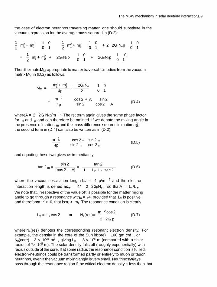
The MSW mechanism in solar neutrino interactions 309
the case of electron neutrinos traversing matter, one should substitute in thevacuum expression for the average mass squared in (D.2):
1
2
(m2
1 + m22
)( 1 00 1
)→ 1
2
(m2
1 + m22
)( 1 00 1
)+ 2
√2GFNep
(1 00 1
)=[
1
2
(m2
1 + m22
)+ √
2GFNep
](1 00 1
)+ √
2GFNep
(1 00 −1
)Then the matrix MM appropriate to matter traversal is modified from the vacuummatrix MV in (D.2) as follows:
MM =[(
m21 + m2
2
)4p
+√
2GFNe
2
](1 00 1
)
+[�m2
4p
]( − cos 2θ + A sin 2θ
sin 2θ cos 2θ − A
)(D.4)
where A = 2√
2GFNep/�m2. The first term again gives the same phase factorfor νe and νμ and can therefore be omitted. If we denote the mixing angle inthe presence of matter as θm and the mass difference squared in matter as �m2
m,the second term in (D.4) can also be written as in (D.2):[
�m2m
4p
]( − cos 2θm sin 2θm
sin 2θm cos 2θm
)(D.5)
and equating these two gives us immediately
tan 2θm = sin 2θ
[cos 2θ − A]= tan 2θ[
1 − (Lv/
Le)
sec 2θ] (D.6)
where the vacuum oscillation length is Lv = 4πp/�m2 and the electron
interaction length is defined as Le = 4π/(
2√
2GFNe
), so that A = Lv/Le.
We note that, irrespective of the value of θ, it is possible for the matter mixingangle to go through a ‘resonance’ with θm = π/4, provided that Lv is positiveand therefore �m2 > 0, that is m2 > m1. The resonance condition is clearly
Lv = Le cos 2θ or Ne(res) = �m2 cos 2θ(2√
2GFp) (D.7)
where Ne(res) denotes the corresponding ‘resonant’ electron density. Forexample, the density in the core of the Sun is ρ (core) ∼ 100 gm cm−3, orNe(core) ∼ 3 × 1031 m−3, giving Le ∼ 3 × 10⁵ m (compared with a solarradius of 7 × 10⁸ m). The solar density falls off (roughly exponentially) withradius outside of the core. If at some radius the ‘resonance’condition is fulfilled,electron-neutrinos could be transformed partly or entirely to muon– or tauon–neutrinos, even if the vacuum mixing angle is very small. Neutrinos will alwayspass through the resonance region if the critical electron density is less than that
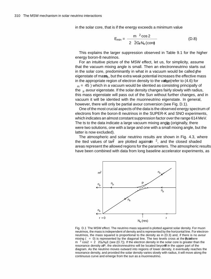
310 The MSW mechanism in solar neutrino interactions
in the solar core, that is if the energy exceeds a minimum value
Emin = �m2 cos 2θ[2√
2GFNe (core)] (D.8)
This explains the larger suppression observed in Table 9.1 for the higherenergy boron-8 neutrinos.
For an intuitive picture of the MSW effect, let us, for simplicity, assumethat the vacuum mixing angle is small. Then an electron–neutrino starts outin the solar core, predominantly in what in a vacuum would be called the ν1
eigenstate of mass m1, but the extra weak potential increases the effective massin the appropriate region of electron density to the value m2, (refer to (4.6) forθm = 45◦) which in a vacuum would be identified as consisting principally ofthe νμ flavour eigenstate. If the solar density changes fairly slowly with radius,this mass eigenstate will pass out of the Sun without further changes, and invacuum it will be identified with the muon–neutrino eigenstate. In general,however, there will only be partial flavour conversion (see Fig. D.1).
One of the most crucial aspects of the data is the observed energy spectrum ofelectrons from the boron-8 neutrinos in the SUPER-K and SNO experiments,which indicates an almost constant suppression factor over the range 6–14 MeV.The fits to the data indicate a large vacuum mixing angle θ12 (originally, therewere two solutions, one with a large and one with a small mixing angle, but thelatter is now excluded).
The atmospheric and solar neutrino results are shown in Fig. 4.3, wherethe fitted values of tan2θ are plotted against �m2, and the closed shadedareas represent the allowed regions for the parameters. The atmospheric resultshave been combined with data from long baseline accelerator experiments, as
P
r = 0 rNe (res)
m2ν
nμ
nμ
nμ
ne
ne
ne
Fig. D.1 The MSW effect. The neutrino mass squared is plotted against solar density. For muon–neutrinos, the mass is independent of density and is represented by the horizontal line. For electron-neutrinos, the mass squared is proportional to the density as in (D.3) and, if there is no flavourmixing (θ = 0) is represented by the diagonal line. The two levels cross at the point P, where�m2 cos2θ = 2
√2GFNeE (see (D.7)). If the electron density in the solar core is greater than the
‘resonance density’ at P, the electron–neutrino will be located beyond P in the upper part of thediagram. As the neutrino moves outward into regions of lower density, it eventually reaches theresonance density, and provided the solar density varies slowly with radius, it will move along thecontinuous curve and emerge from the sun as a muon–neutrino.

The MSW mechanism in solar neutrino interactions 311
described above, while the solar data on νe have been combined with thosefrom νe beams (assuming the validity of CPT), for example the KAMLANDexperiment at the Kamioka mine site, using reactor antineutrinos on ∼200 kmbaseline. Of course, the reactor experiments measure the value of the vacuummixing angle θ12 directly, and have short enough path lengths that they areuntroubled by matter effects.
Answers to problems
Answers are given to all the problems. Fully worked solutions are given forthose problems marked with an asterisk.
Chapter 1
(1.1)(GM 2
/R/2Mc2
): 2.5 × 10⁻¹⁴; 8 × 10⁻²¹.
(1.2) In terms of quarks the reaction is written as follows:
du + udu → uds + ds
The strong interactions have a range of order r0 = 1 fm, hence atypical cross-section of σ = πr2
0 = 31 mb (= 3.1 × 10⁻²⁶ cm2).The characteristic time is r0/c = 3 × 10⁻²⁴s. Thus a value of σ = 1mb corresponds to a strong-interaction time in this case of 10−23 s.
Hence the ratio of weak coupling to strong coupling is(10−23/10−10
)1/2
∼ 10−6.(1.3) 29.8 MeV: 10 GeV: 5.7 GeV.(1.4) 5.5 × 10⁻²⁴ s; 134 fm.(1.5) (a) yes; (b) and (c) no, �S = 2 forbidden to first order in coupling; (d)
no, because of energy conservation.(1.6) If all final state lepton masses are neglected, the rate is proportional to
Q5. In nuclear beta decay, this is known as the Sargent Rule. The decayrate W in (1.15) has dimensions E−1. The formula includes a factor E−4
from the weak coupling G2F as in (1.27). Hence the other factors in the
expression for W must have dimensions E5, that is vary as Q5 as Q isthe important energy in the problem. The values of W/Q5 in MeV−5 s−1
are as follows:
(a) 3.5×10⁻⁵ (b) 3.6×10⁻⁵ (c) 3.4×10⁻⁴ (d) 2.7×10⁻⁴ (e) 3.9×10⁻³.The extreme relativistic approximation for the electron secondarydoes not hold for processes (c), (d), and (e) and W/Q5 shows anincrease with decreasing Q.
(1.7) We start by considering a massless neutrino of very high energy E,momentum p colliding with a nucleon of mass M at rest. The square
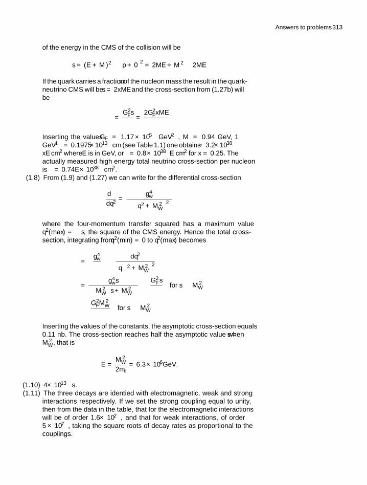
Answers to problems 313
of the energy in the CMS of the collision will be
s = (E + M )2 − (p + 0)2 = 2ME + M 2 ∼ 2ME
If the quark carries a fraction x of the nucleon mass the result in the quark-neutrino CMS will be s = 2xME and the cross-section from (1.27b) willbe
σ = G2Fs
π= 2G2
FxME
π
Inserting the values GF = 1.17 × 10⁻⁵ GeV−2, M = 0.94 GeV, 1GeV−1 = 0.1975×10⁻¹³ cm (see Table 1.1) one obtains σ = 3.2×10−38
xE cm2 where E is in GeV, or σ = 0.8 × 10−38E cm2 for x = 0.25. Theactually measured high energy total neutrino cross-section per nucleonis σ = 0.74E × 10−38 cm2.
(1.8) From (1.9) and (1.27) we can write for the differential cross-section
dσ
dq2= g4
w[π(q2 + M 2
W
)2]where the four-momentum transfer squared has a maximum valueq2(max) = − s, the square of the CMS energy. Hence the total cross-section, integrating from q2(min) = 0 to q2(max) becomes
σ =(
g4w
π
)∫dq2[−q2 + M 2
W
]2= g4
ws[πM 2
W
(s + M 2
W
)] → G2F s
πfor s M 2
W
→ G2FM 2
W
πfor s � M 2
W
Inserting the values of the constants, the asymptotic cross-section equals0.11 nb. The cross-section reaches half the asymptotic value when s =M 2
W , that is
E = M 2W
2me= 6.3 × 10⁶GeV.
(1.10) 4 × 10⁻¹³ s.(1.11) The three decays are identified with electromagnetic, weak and strong
interactions respectively. If we set the strong coupling equal to unity,then from the data in the table, that for the electromagnetic interactionswill be of order 1.6 × 10⁻², and that for weak interactions, of order5 × 10−7, taking the square roots of decay rates as proportional to thecouplings.
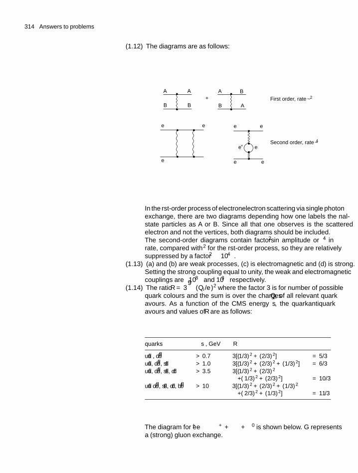
314 Answers to problems
(1.12) The diagrams are as follows:
A
e e
A�
B B�
A B�
B A�
�
� e
e e
e+ e–
e�
�
�
�
�
e � �
γ
γ γ
�
�
�
+ First order, rate ~ �2
Second order, rate ~ �4
In the first-order process of electron–electron scattering via single photonexchange, there are two diagrams depending how one labels the final-state particles as A or B. Since all that one observes is the scatteredelectron and not the vertices, both diagrams should be included.The second-order diagrams contain factors α2 in amplitude or α4 inrate, compared with α2 for the first-order process, so they are relativelysuppressed by a factor α2 ∼ 10−4.
(1.13) (a) and (b) are weak processes, (c) is electromagnetic and (d) is strong.Setting the strong coupling equal to unity, the weak and electromagneticcouplings are ∼ 10−8 and 10−3 respectively.
(1.14) The ratio R = 3∑
(Qi/e)2 where the factor 3 is for number of possiblequark colours and the sum is over the charges Qi of all relevant quarkflavours. As a function of the CMS energy
√s, the quark–antiquark
flavours and values of R are as follows:
quarks√
s , GeV R
uu , dd > 0.7 3[(1/3)2 + (2/3)2] = 5/3uu, dd, ss > 1.0 3[(1/3)2 + (2/3)2 + (1/3)2] = 6/3uu, dd, ss, cc > 3.5 3[(1/3)2 + (2/3)2
+(1/3)2 + (2/3)2] = 10/3uu dd, ss, cc, bb > 10 3[(1/3)2 + (2/3)2 + (1/3)2
+(2/3)2 + (1/3)2] = 11/3
The diagram for e+e− → π+ + π− + π0 is shown below. G representsa (strong) gluon exchange.
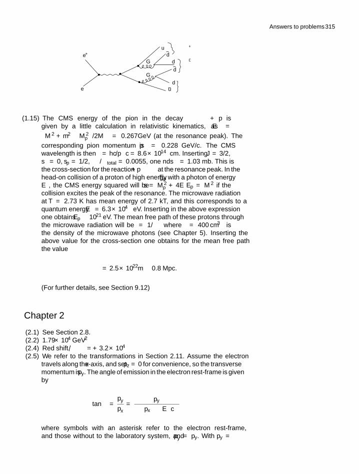
Answers to problems 315
G
u π+
π0
π–
u
dd
d
G
e+
e–
γ d
(1.15) The CMS energy of the pion in the decay � → π + p isgiven by a little calculation in relativistic kinematics, as Eπ =(
M 2� + m2
π − M 2p
)/2M� = 0.267GeV (at the resonance peak). The
corresponding pion momentum is pπ = 0.228 GeV/c. The CMSwavelength is then λπ = hc/pπc = 8.6 × 10⁻¹⁴cm. Inserting J = 3/2,sπ = 0, sp = 1/2, �γ/�total = 0.0055, one finds σ = 1.03 mb. This isthe cross-section for the reaction γ+p → � at the resonance peak. In thehead-on collision of a proton of high energy Ep with a photon of energyEγ , the CMS energy squared will be s = M 2
p + 4EγEp = M 2� if the
collision excites the peak of the � resonance. The microwave radiationat T = 2.73 K has mean energy of 2.7 kT, and this corresponds to aquantum energy Eγ = 6.3 × 10⁻⁴ eV. Inserting in the above expressionone obtains Ep ∼ 1021 eV. The mean free path of these protons throughthe microwave radiation will be λ = 1/ρσ where ρ = 400 cm−3 isthe density of the microwave photons (see Chapter 5). Inserting theabove value for the cross-section one obtains for the mean free paththe value
λ = 2.5 × 10²²m ∼ 0.8 Mpc.
(For further details, see Section 9.12)
Chapter 2
(2.1) See Section 2.8.(2.2) 1.79 × 10⁴ GeV2
(2.4) Red shift, �λ/λ = +3.2 × 10⁻⁴
(2.5) We refer to the transformations in Section 2.11. Assume the electrontravels along the x-axis, and set pz = 0 for convenience, so the transversemomentum is py. The angle of emission in the electron rest-frame is givenby
tan θ∗ = p∗y
p∗x
= py[γ(px − βE
/c)]
where symbols with an asterisk refer to the electron rest-frame,and those without to the laboratory system, and p∗
y = py. With py =
316 Answers to problems
p sin θ , px = p cos θ, and E = pc for a photon one obtains
tan θ∗ = sin θ
[γ (cos θ − β)]
In the electron rest-frame, half of the photons will have θ∗ < π/2, orcos θ > β, or sin θ < 1/γ . For ultra-relativistic particles, the half-widthof the beam of emitted photons is therefore θ ∼ 1/γ .
(2.6) Gravitational shift = +5.28 × 10⁻¹⁰.Special relativity shift = −0.63 × 10⁻¹⁰.Net shift = +4.45 × 10⁻¹⁰.
= 38μs/day (satellite clock runs fast).
Chapter 3
(3.2) Positive and negative pions are particle and antiparticle. Positive andnegative sigma baryons are not.
(3.3) ρ- meson has C = P = −1. f-meson has C = P = +1. The processρ → π0γ is allowed as an electromagnetic decay, with a branching ratio∼ α (actually 0.07%). Corresponding decay for f-meson is forbidden byC-invariance.
(3.5) If pe, Ee, me, and pp, Ep,and Mp refer to the three-momenta, total energiesand masses of the electron and proton respectively, then the square ofthe total four-momentum, equal to the CMS energy squared, is (seeSection 2.11):
s = (Ee + Ep)2 − (pe + pp
)2 = m2e + m2
p
+ 2(EeEp − pe · pp
) ≈ 4EeEp
where in the final step we have used the fact that both particles are extremerelativistic, so that masses can be neglected, and the fact that the electronand proton momenta are in opposite directions.
(a) Inserting numbers, the value of s = 98, 400 GeV2.(b) The CMS energy squared of the electron-quark system is s/4.(c) The cross-section for the electromagnetic interaction is given by
(1.23), which assumes that q2 q2max = s. In this approximation
(dσ
dq2
)em
= 4πα2 |Q/e|2q4
(i)
where |Q/e| = 2/3 is the u-quark charge. The cross-section for theweak charged-current interaction is given by (1.23b) which, after
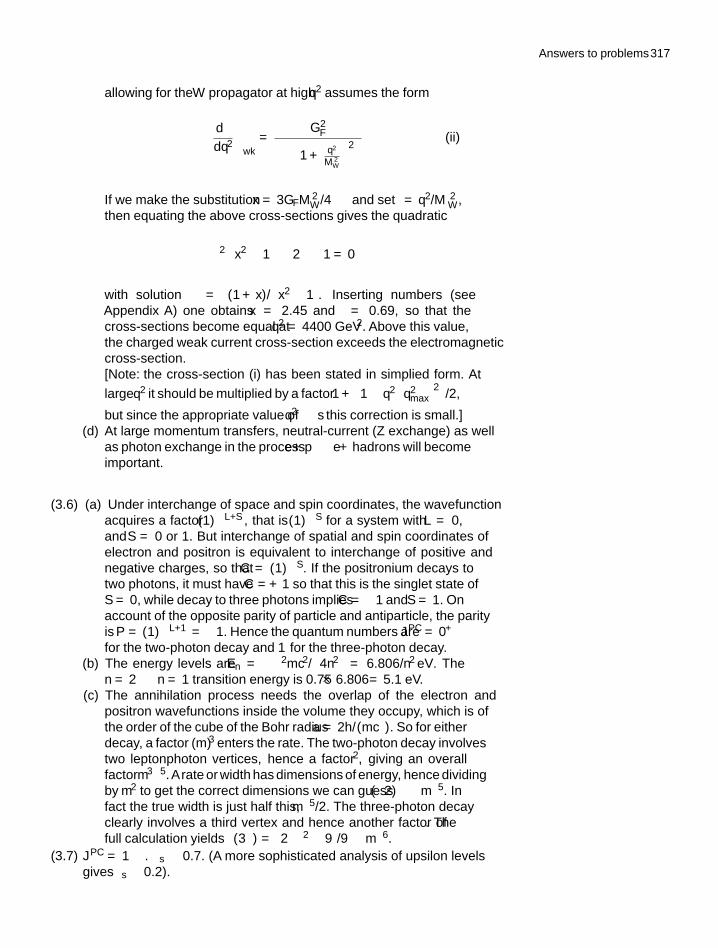
Answers to problems 317
allowing for the W propagator at high q2 assumes the form
(dσ
dq2
)wk
= G2F[
π(
1 + q2
M 2W
)2] (ii)
If we make the substitution x = 3GFM 2W /4πα and set γ = q2/M 2
W ,then equating the above cross-sections gives the quadratic
γ2(
x2 − 1)
− 2γ − 1 = 0
with solution γ = (1 + x)/(x2 − 1
). Inserting numbers (see
Appendix A) one obtains x = 2.45 and γ = 0.69, so that thecross-sections become equal at q2 = 4400 GeV2. Above this value,the charged weak current cross-section exceeds the electromagneticcross-section.[Note: the cross-section (i) has been stated in simplified form. At
large q2 it should be multiplied by a factor[1 + (1 − q2
/q2
max
)2]/2,
but since the appropriate value of q2 s this correction is small.](d) At large momentum transfers, neutral-current (Z exchange) as well
as photon exchange in the process e+p → e+ hadrons will becomeimportant.
(3.6) (a) Under interchange of space and spin coordinates, the wavefunctionacquires a factor (−1)L+S , that is (−1)S for a system with L = 0,and S = 0 or 1. But interchange of spatial and spin coordinates ofelectron and positron is equivalent to interchange of positive andnegative charges, so that C = (−1)S . If the positronium decays totwo photons, it must have C = +1 so that this is the singlet state ofS = 0, while decay to three photons implies C = −1 and S = 1. Onaccount of the opposite parity of particle and antiparticle, the parityis P = (−1)L+1 = −1. Hence the quantum numbers are J PC = 0−+for the two-photon decay and 1−− for the three-photon decay.
(b) The energy levels are En = −α2mc2/(4n2) = 6.806/n2 eV. The
n = 2 → n = 1 transition energy is 0.75 × 6.806 = 5.1 eV.(c) The annihilation process needs the overlap of the electron and
positron wavefunctions inside the volume they occupy, which is ofthe order of the cube of the Bohr radius a = 2h/(mcα). So for eitherdecay, a factor (mα)3 enters the rate. The two-photon decay involvestwo lepton–photon vertices, hence a factor α2, giving an overallfactor m3α5. Arate or width has dimensions of energy, hence dividingby m2 to get the correct dimensions we can guess �(2γ) ∼ mα5. Infact the true width is just half this, mα5/2. The three-photon decayclearly involves a third vertex and hence another factor of α. Thefull calculation yields � (3γ) = [2 (π2 − 9
)/9π]
mα6.(3.7) J PC = 1−−. αs ∼ 0.7. (A more sophisticated analysis of upsilon levels
gives αs ∼ 0.2).
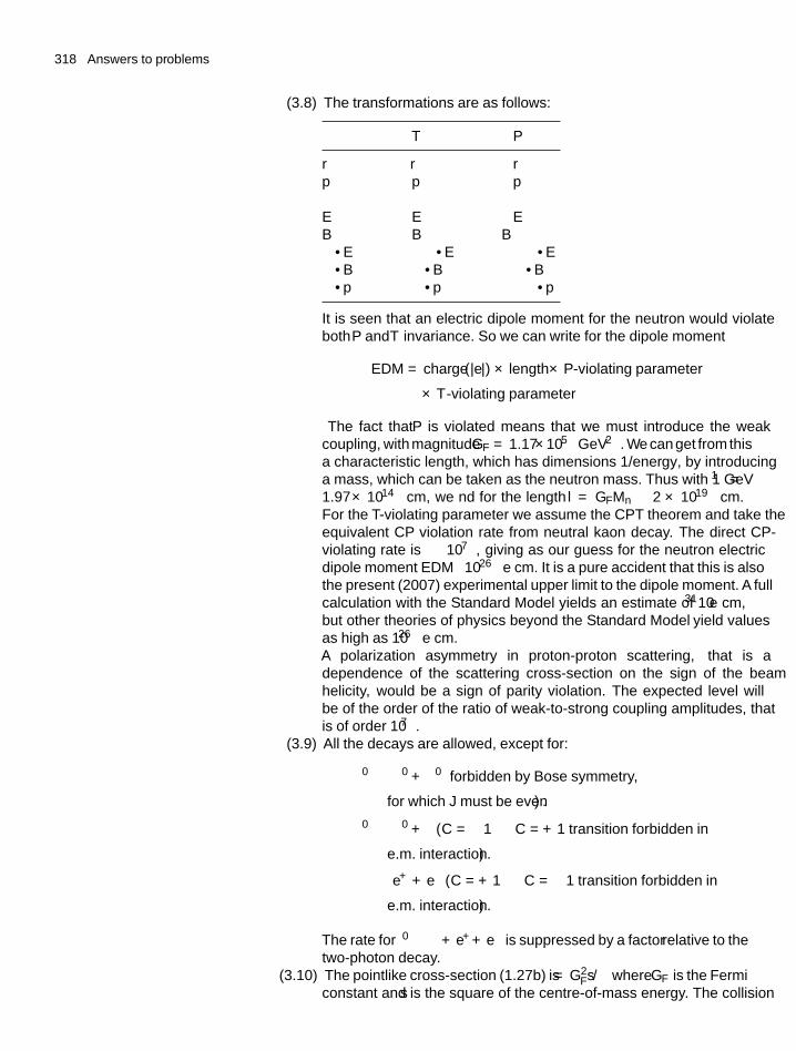
318 Answers to problems
(3.8) The transformations are as follows:
T P
r r −rp −p −pσ −σ σ
E E −EB −B Bσ · E −σ · E −σ · Eσ · B σ · B σ · Bσ · p σ · p −σ · p
It is seen that an electric dipole moment for the neutron would violateboth P and T invariance. So we can write for the dipole moment
EDM = charge (|e|) × length × P-violating parameter
× T -violating parameter
The fact that P is violated means that we must introduce the weakcoupling, with magnitude GF = 1.17×10⁻⁵ GeV−2. We can get from thisa characteristic length, which has dimensions 1/energy, by introducinga mass, which can be taken as the neutron mass. Thus with 1 GeV−1 =1.97 × 10⁻¹⁴ cm, we find for the length l = GFMn ∼ 2 × 10⁻¹⁹ cm.For the T-violating parameter we assume the CPT theorem and take theequivalent CP violation rate from neutral kaon decay. The direct CP-violating rate is ε′ ∼ 10−7, giving as our guess for the neutron electricdipole moment EDM ∼ 10−26 e cm. It is a pure accident that this is alsothe present (2007) experimental upper limit to the dipole moment. A fullcalculation with the Standard Model yields an estimate of 10−31 e cm,but other theories of ‘physics beyond the Standard Model’ yield valuesas high as 10−26 e cm.A polarization asymmetry in proton-proton scattering, that is adependence of the scattering cross-section on the sign of the beamhelicity, would be a sign of parity violation. The expected level willbe of the order of the ratio of weak-to-strong coupling amplitudes, thatis of order 10−7.
(3.9) All the decays are allowed, except for:
ρ0 → π0 + π0 (forbidden by Bose symmetry,
for which J must be even) .
ρ0 → π0 + η (C = −1 → C = +1 transition forbidden in
e.m. interaction) .
η → e+ + e− (C = +1 → C = −1 transition forbidden in
e.m. interaction) .
The rate for π0 → γ+ e++ e− is suppressed by a factor α relative to thetwo-photon decay.
(3.10) The pointlike cross-section (1.27b) is σ = G2Fs/π where GF is the Fermi
constant and s is the square of the centre-of-mass energy. The collision
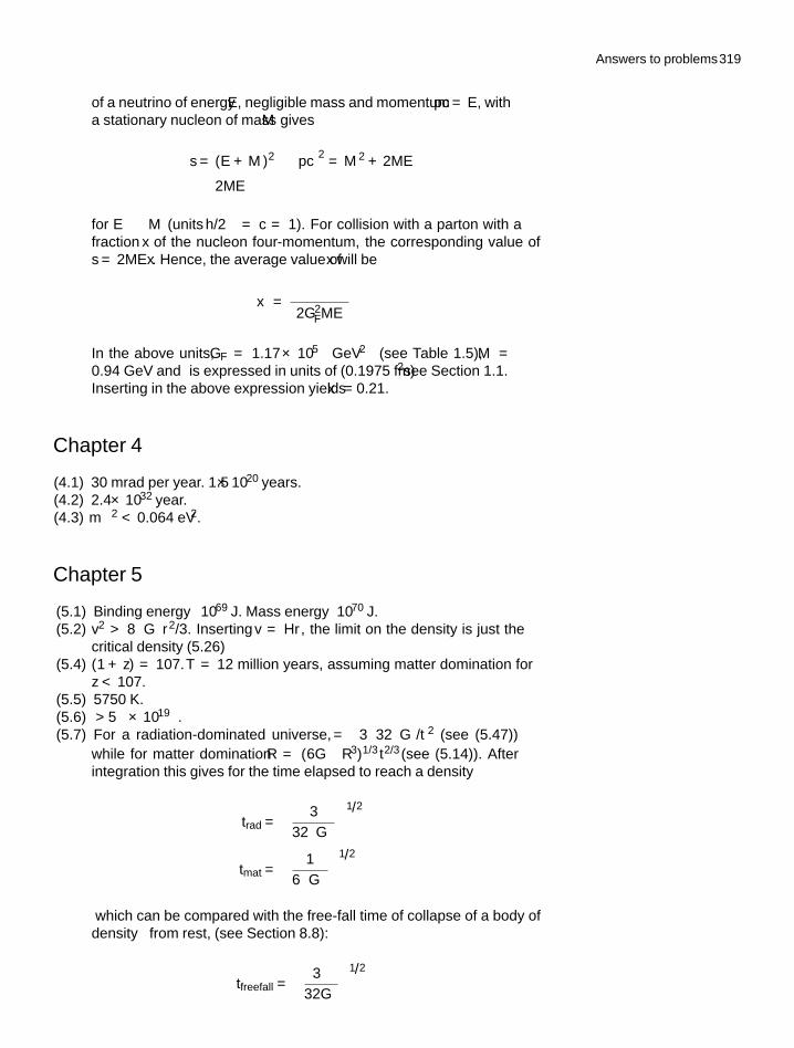
Answers to problems 319
of a neutrino of energy E, negligible mass and momentum pc = E, witha stationary nucleon of mass M gives
s = (E + M )2 − (pc)2 = M 2 + 2ME
≈ 2ME
for E � M (units h/2π = c = 1). For collision with a parton with afraction x of the nucleon four-momentum, the corresponding value ofs = 2MEx. Hence, the average value of x will be
〈x〉 = πσ(2G2
FME)
In the above units, GF = 1.17 × 10⁻⁵ GeV−2 (see Table 1.5), M =0.94 GeV and σ is expressed in units of (0.1975 fm)2—see Section 1.1.Inserting in the above expression yields 〈x〉 = 0.21.
Chapter 4
(4.1) 30 mrad per year. 1.5 × 10²⁰ years.(4.2) 2.4 × 1032 year.(4.3) �m2 < 0.064 eV2.
Chapter 5
(5.1) Binding energy ∼ 1069 J. Mass energy ∼ 1070 J.(5.2) v2 > 8πGρr2/3. Inserting v = Hr, the limit on the density is just the
critical density (5.26)(5.4) (1 + z) = 107. T = 12 million years, assuming matter domination for
z < 107.(5.5) 5750 K.(5.6) ε > 5 × 10⁻¹⁹.(5.7) For a radiation-dominated universe, ρ = (
3/
32πG)/t2 (see (5.47))
while for matter domination R = (6GπρR3)1/3t2/3(see (5.14)). Afterintegration this gives for the time elapsed to reach a density ρ
trad =(
3
32πGρ
)1/2
tmat =(
1
6πGρ
)1/2
which can be compared with the free-fall time of collapse of a body ofdensity ρ from rest, (see Section 8.8):
tfreefall =(
3π
32Gρ
)1/2
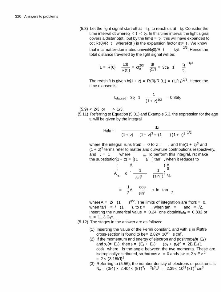
320 Answers to problems
(5.8) Let the light signal start off at t = t1, to reach us at t = t0. Consider thetime interval dt′ where t1 < t′ < t0. In this time interval the light signalcovers a distance cdt′, but by the time t = t0, this will have expanded tocdt′R (0)/R
(t′)
where R(t′) is the expansion factor at t = t′. We know
that in a matter-dominated universe R (0)/R(t′) = (t0/t′
)2/3. Hence the
total distance travelled by the light signal will be:
L = R (0)
∫cdt′
R (t′)= ct2/3
0
∫dt′
t′2/3= 3ct0
[1 −(
t1t0
)1/3]
The redshift is given by (1 + z) = R (0)/R (t1) = (t0/t1)2/3. Hence thetime elapsed is
telapsed = 3t0
[1 − 1
(1 + z)1/2
]= 0.85t0.
(5.9) < 2/3, or �λ > 1/3.(5.11) Referring to Equation (5.31) and Example 5.3, the expression for the age
t0 will be given by the integral
H0t0 =∫
dz
(1 + z)[� (1 + z)3 + (1 − �) (1 + z)2]1/2
where the integral runs from z = 0 to z = ∞, and the (1 + z)3 and(1 + z)2 terms refer to matter and curvature contributions respectively,and �k = 1 − � where � ≡ �m. To perform this integral, first makethe substitution (1 + z) = [(1 − �)/�] tan2 θ, when it reduces to
A
⎧⎨⎩∫
dθ
⎡⎣ 1(sin3 θ
) − 1
(sin θ)
⎤⎦⎫⎬⎭= −1
2A
{(cos θ
sin2 θ
)+ ln
[tan
(θ
2
)]}where A = 2�/(1 − �)3/2. The limits of integration are from z = 0,when tan2 θ = �/(1 − �), to z = ∞, when tan2θ = ∞ and θ = π/2.Inserting the numerical value � = 0.24, one obtains H0t0 = 0.832 ort0 = 11.3 Gyr.
(5.12) The stages in the answer are as follows:
(1) Inserting the value of the Fermi constant, and with s in MeV2, thecross-section is found to be σ = 2.82 × 10−45 s cm2.
(2) If the momentum and energy of electron and positron are p1(= E1)
and p2(= E2), then s = (E1 + E2)2 − (p1 + p2)
2 = 2E1E2(1 −cos θ) where θ is the angle between the two momenta. These areisotropically distributed, so that<cosθ> = 0 and <s> = 2 <E >2
= 2 × (3.15kT )2.(3) Referring to (5.56), the number density of electrons or positrons is
Ne = (3/4) × 2.404 × (kT )3/(π2h3c3
) = 2.39 × 1031 (kT )3 cm−3
Answers to problems 321
(with kT in MeV). Setting the relative velocity v ∼ c, the value of1/W = 1/〈σNev〉 ∼ 25/(kT )5s.
(4) From (5.49) and (5.58) one obtains t=0.74/(kT )2s for g∗=43/4.Equating t with 1/W gives for the freeze-out temperature kT∼3 MeV.
[Note: This is only an approximate value, for several reasons. First,the calculation of both cross-sections and particle densities assumes allparticles are extreme relativistic, and the corrections for electron masswill reduce the cross-section, the particle density and the relative velocityand thus increase the freeze-out temperature. Second, the calculationof the cross-section ignores the effects of Z0-exchange (neutral weakcurrents) which will increase it by about 15% and hence reduce thecritical temperature].
Chapter 6
(6.1) As indicated in Chapter 5, the freeze out of neutrons and protonsfrom equilibrium occurs when the interaction rate W in (6.1), varyingas T 5, falls below the expansion rate H in (5.59), varying as T 2
g∗1/2. Thus the freeze-out temperature T ∝ g∗1/6
, where g∗ =(22 + 7Nv)/4 is the number of states of photons, electrons, positrons,and neutrinos/antineutrinos and Nν is the number of neutrino families(see Section 5.10). For Nν = 3, g∗ = 43/4, kT = 0.8 MeV, so that kTfor other values of Nν is easily found. Inserting in (6.4), the initial andfinal neutron/proton ratios and hence the helium mass fraction can becalculated as a function of the assumed number of neutrino families.For a neutron–proton mass difference of 1.4 MeV and three neutrinoflavours, the initial neutron/proton density ratio in (6.5) becomes 0.174,leading to a helium mass fraction of 0.21.
(6.2) Referring to equation (1.18) the cross-section for the reaction νe + n →e− + p is given by the approximate formula (putting |Tif |2 = G2
F):
σ =(
1
πh4c4
)G2
F
(pf c)2
where we have taken vi = vf = c. With GF = 1.17 × 10⁻⁵ (hc)3 GeV−2
this gives σ = 1.69(pf c)2 × 10−44 cm2 with the final state momentumpf c in MeV. The width or rate for the reaction per neutron target is foundfrom (1.14) as W = σφ where φ = nc is the flux of incident neutrinosand n is their number density as given by (5.50) and (5.56), that is φ =2 × 1042(kT )3 in units cm−2 s−1, with kT measured in MeV. This gives avalue of W = 0.05(kT )3(pf c)2 s−1, to be compared with H = 0.7 (kT)2
s−1 from (5.59) for three neutrino flavours. The value of the final statemomentum in the reaction will be pf c ∼ kT + Q where Q = 1.29 MeV.Setting W/H = 1 for the freeze-out condition gives kT ∼ 1.5 MeV, ascan be found by trial and error. This is an overestimate of the freeze-outtemperature for several reasons. First, in assuming equation (1.18) wehave ignored the effects of spin, and that both vector and axial vectorinteractions are involved in the matrix element. This will increase the
322 Answers to problems
cross-section and decrease the freeze out temperature; second, we haveignored the electron mass, which with a value of 0.51 MeV is comparablewith kT; third, an integration should be made over the thermal spectrumand over the isotropic angular distribution of the colliding particles. Whenall such effects are accounted for, the freeze-out temperature is found tobe approximately 0.8 MeV.
(6.3) kT = 0.06 MeV(6.4) 5%
Chapter 7
(7.1) �θ = 2GM /bc2
[Note: This is too small by a factor 2, as compared with the value givenby the general theory of relativity. One reason for the discrepancy is that,in the Newtonian approach, only the spatial coordinates of the photonare considered, while in fact the gravitational field also affects the timecoordinate, as explained in Chapter 2. This introduces a time delay (calledthe Shapiro delay) which must introduce an extra deflection (as is familiarin classical optics, when the speed of light changes as it travels from aless dense to a more dense medium).]
(7.2) v2 = GM
Rv = 210kms−1
Optical depth τ = v2/c2 = 10−6.
(7.3) ER =[
4MDMR
(MD + MR)2
]ED cos2 θ
ER is maximum when θ = 0.
ER(max) = ED when MR = MD.
For MR MD, ER(max) = 4ED
(MR
MD
)For MD MR, ER(max) = 4ED
(MD
MR
).
ER ∼ 70 keV in numerical problem.
(7.4) 1.03 × 10⁻¹¹ m s−2 ∼ 10−12 g.
Chapter 8
(8.1) τ = 2π
ω=(
3π
Gρ
)1/2
(8.2) vs = 360 m s−1,
λJ = 6.88 × 10⁷ m,
MJ = πρλ3J
6= 2.2 × 10²³kg
(cf Earth mass = 6 × 1024kg)
Answers to problems 323
(8.4) t = 3λ2/(c2ti)
λ = 1cm t = 104y M = 1016MS ∼ cluster mass
λ = 1mm t = 102y M = 1012MS ∼ galaxy mass.
(8.6) 14.9 Gpc.(8.7) Consider photons travelling through ionized gas in a flat, expanding
universe. From (5.43) and (5.44) the element of (true) coordinate distancetravelled is related to the red shift interval dz by
dD =(
c
H0
)dz[
�m (0) (1 + z)3 + �r (0) (1 + z)4
+�v (0) + �k (0) (1 + z)2]1/2
Since we will be concerned with z values of around 20 or less, we can to afirst approximation neglect all terms in the denominator of the expressionfor dD except the first. Then the probability that a photon will undergoThomson scattering in traversing this distance will be
dP =[�b (0) (1 + z)3 ρc
]σTN0μ (z) dD
where the product in square brackets gives the baryon—and henceelectron—density at redshift z. ρc is the critical density today, σT is theThomson cross-section for photon–electron scattering in the eV energyregion, N0 is Avogadro’s number, and μ(z) is the degree of ionizationof the intergalactic medium. The integrated scattering probability fromz = z to z = 0 becomes
P =(
c
H0
)�b (0)
[�m (0)]1/2ρcσTN0
∫(1 + z)3/2μ (z) dz
We do not know μ(z), except that it certainly decreases as z increases.For simplicity, let us assume that stars formed at an effective value of z= zs, below which the gas is 100% ionized, so that for z < zs, μ(z) = 1,and μ(z) = 0 for z > zs. Then, assuming P = 0.1 (the value quoted bythe WMAP experiment) and inserting the values of the other constants,one finds zs = 12, which translates to a time of ∼ 0.25 Gyr after the BigBang.
(8.8) vgalaxy ∼ 2.5 × 10⁵ m s−1; vcluster ∼ 4 × 10⁵ m s−1
Neutrino r.m.s. velocities 2.1 × 10⁷, 6.8 × 10⁶, and 2.1 × 10⁶ m s−1
respectively.(8.9) From (5.32) we take for the present baryon density, assuming it to be
dominated by protons, the value of 0.24 protons m−3, which is alsothe electron density Ne(0). At the time of decoupling (zdec ∼ 1100) theelectron density would be Ne(dec) = Ne(0)(1 + zdec)
3. The Thomsoncross-section (1.26d) is σTh = 6.7×10⁻²⁹ m2, giving a mean free path forCMB photons of λTh = 1/(Neσ) = 4.7 × 10¹⁹m = 1.51kpc, assumingthe medium to be totally ionized. Since near z = 1100, baryonic matter isonly partly ionized, we take a value of 10λ as illustrative of the thicknessof this ‘last scattering shell’.
324 Answers to problems
From (5.43) and (5.44), and assuming a flat universe (k = 0) withdominance of matter over radiation and vacuum energy, as expectedfor z ∼ 1100, we obtain the value of the shell thickness �D related tothe corresponding interval �z as follows:
�D ∼(
c
H0
)dz[�m (0) (1 + zdec)
3]−1/2 = 8.1 × 10²¹�z m
Equating this to the present thickness of the last scattering shell, 10λTh(1 + zdec) = 5.16 × 10²³ m, one obtains �z ∼ 64. This correspondsto an angular uncertainty �θ ∼ 0.03◦, from (8.64), and the smearing outof peaks at such small angles.
Chapter 9
(9.1) E−2.22.(9.2) 110 m.(9.3) 2.4 km.(9.4) The probability that a pion is produced in an element dx at depth x g
cm−2 in the atmosphere by a primary proton is exp (−x/λ) dx/λ, wherethe interaction length λ ∼ 100 g cm−2. The probability that it will thensurvive to depth y without interaction is exp
[−(x − y)/λ], where to keep
the problem simple we assume the same interaction length for pions andprotons.The connection between the depth x in g cm−2 and height h is h =H ln (X /x), where X = 1030 g cm−2 is the total atmospheric depth,and again for simplicity we have assumed an isothermal, exponentialatmosphere (strictly only true in the top third of the atmosphere) withH = 6.5 km.In traversing the interval x to y the pion covers a distance s = Hln(y/x), and the probability that it does this without decaying, and
subsequently decays in an element ds is
dP = exp
( −s
γcτ
)ds
γcτ=(
H
γcτ
)·(
dy
y
)· exp
[−(
H
γcτ
)ln(y
x
)]= α
(x
y
)α dy
y
where α = H/γcτ = Eo/E. Here E is the pion energy, γ = E/mc2 andm and τ are the pion mass and mean lifetime. Thus the joint probabilitythat a pion is created in dx and survives to decay in the depth intervaldy is
P(x, y)
dx dy =(
dx
λ
)exp
(−x
λ
)exp
[−(x − y
)λ
]α
(x
y
)α dy
y
and the probability that the pion is produced at any value of x < y anddecays in dy is found by straightforward integration to be
P(y)
dy =[
α
(α + 1)
]exp(− y
λ
) dy
λ
Answers to problems 325
The overall probability that the pion decays anywhere in the atmosphereis found by integrating from y = 0 to y = X . Since X � λ the yintegration just gives unity. So the overall pion decay probability is
Pdecay = α
(α + 1)= E0
(E + E0)
where E0 = Hmc2/cτ = 117GeV.If the pion is produced at a zenith angle θ, depths remain the same, butall distances are multiplied by the secant of this angle, so that the energyE0 is simply replaced by E0secθ.
(9.5) No CP-violating effects are possible with only two flavours in vacuum,since a CP-violating phase requires at least three flavours and a 3 ×3mixing matrix. If matter effects in the Earth are taken into account,induced CP-violating effects, that is a difference in the oscillationamplitudes for neutrinos and antineutrinos are possible with only twoneutrino flavours, because the Earth is not CP-symmetric, being madeof matter without antimatter. (see also Appendix D).
(9.6) Applying the conservation of energy and the conservation of momentum,parallel, and perpendicular to the direction of the incident neutrino,allows one to eliminate the energy and angle of emission of the recoilelectron, and there results a relation between the angle of emission θ ofthe scattered neutrino and its energy, E′, in terms of the incident energyE:
cos θ = 1 − m
(1
E′ − 1
E
)where m is the electron mass, and the neutrino is assumed massless.Since E � m, we can expand cos θ ≈ 1 − θ2/2, whence we obtain therelation
θ =√
2m
(1
E′ − 1
E
)(9.7) Applying the energy and momentum transformations in Section 2.11,
one obtains values for the energy and momentum, E* and p*, of themuon in the pion rest-frame:
E∗ =(m2
π + m2μ
)2mπ
; p∗ =(m2
π − m2μ
)2mπ
and for the laboratory energy of the muon from decay of a relativisticpion of Lorentz factor γ = Eπ/mπ and β ≈ 1 the value
Eμ = γ(E∗ + p∗ cos θ∗)
where θ* is the angle of emission of the muon in the pion rest-frame. Because the pion has spin zero, this angular distribution isisotropic, and the muon energy in the laboratory therefore extends from(m2
μ/m2π
)Eπ = 0.58Eπ to Eπ, with a mean value of 0.79Eπ. Hence the
neutrino receives an average energy of 0.21Eπ. In its subsequent decay,the muon transforms into a positron, an electron–neutrino and a muon–antineutrino, each receiving approximately one-third of the muon energy,
326 Answers to problems
that is about 0.26Eπ. In summary, therefore, the average energies of thevarious neutrinos are as follows:
π+ → μ+ + vμ
⟨E(vμ
)⟩ = 0.21Eπ
μ+ → e+ + ve + vμ 〈E (ve)〉 = ⟨E (vμ
)⟩ = 0.26Eπ
The numbers here ignore the effects of spin polarization of the muonsfrom pion decay, which can affect the mean energies by several percent.
(9.8) P = 5 microwatts.(9.10) 3 × 10⁻⁴.(9.13) Suppose the jet of relativistic particles emits a light signal at time t0 and
a second signal at time (t0 +�t). Taking the x-axis as the line of sight tothe Earth and the y-axis in the transverse direction, the actual transversevelocity of the jet is �y/�t = v sin θ, but this is not the value observed atthe Earth. Since the jet is moving towards the Earth with velocity v cos θ,the time on the Earth between the two signals is
�tE = �t − �x
c= �t
[1 −(v
c
)cos θ]
.
Hence the apparent transverse velocity measured on the Earth is
utrans
c= �y
c�tE= β sin θ
(1 − β cos θ)
where β = v/c and γ = 1/
√(1 − β2
). Differentiation shows that
utrans/c has a maximum value of γβ when sin θ = 1/γβ, and thereforeexceeds unity when β > 1/
√2. On the contrary, when θ > π/2, the
‘away jet’ will be observed to have a transverse velocity less than β sinθ.
Chapter 10
(10.1) ω = 0.63 rd s−1.(10.2) 5 billion years.(10.3) If the mass M is to be supported by degeneracy pressure, the density is
given by (10.29):
ρdeg =(
4m3e
h6
)(AmP
Z
)5 (4π
3
)3
M 2G3
If M is small enough, ρdeg will fall below normal solid matter densitiesand atomic (electromagnetic) forces will then prevent gravitationalcollapse. So the maximum mass not dependent on electron degeneracyfor stability is found by setting ρdeg = ρmatter = 104 kg m−3. Insertingthe various constants yields M ∼ 5 × 1027 kg or about 0.25 % ofthe solar mass. The largest planet in the solar system is Jupiter withM = 0.001Msun, for which the increase in central density due toelectron degeneracy would be only about 10%.
(10.4) t < 660 years, inconsistent with its origin in 1054 A.D.
Answers to problems 327
(10.5) The particle horizon distance is nct0 where n = 2 for a radiation-dominated universe and n = 3 for matter-domination. If the mass is M ,then
rs = 2GM
c2= nct0
or MBH = nc3t02G
The mass of the universe of age t0 and critical density is(4π/3) ρc (nct0)3. Inserting the values in SI units of ρc = 9 × 10⁻²⁷
and G = 6.7 × 10⁻¹¹, this is equal to the above mass when t0 =1.5 × 10¹⁰/nyears.
(10.6) R ∼ 10−15 m (about equal to the radius of a proton).M ∼ 1012 kg (about equal to the mass of a typical mountain).(Inserting all the constants in (10.51) gives t = 8.1 × 1066
(M /Msun)3 years. And equating to the age of 14 billion years gives
M = 2.41 × 10¹¹ kg and R = 7.4 × 10⁻¹⁶ m.)(10.8) For an elliptic orbit with semi-major axis a and eccentricity e, the
velocity of the star in orbit at radius vector r is given by v2 =GM [(2/r) − 1/a] where M is the mass of the black hole, situatedat the focus of the ellipse. At the perigee, r = a(1 - e) andv2 = (GM /a) [(1 + e)/(1 − e)], while the period of the orbit is givenby Kepler’s Law as τ2 = 4π2a3/[GM ]. Inserting the value of theeccentricity e = 0.87, period τ = 15years = 4.7 × 10⁸ s, andthe perigee distance as 17 lighthours = 1.84 × 10¹³ m, we obtaina = 1.4 × 10¹⁴ m, M = 3.65 × 10⁶Msun, and the velocity of the star atperigee as v = 7170 km per s.

This page intentionally left blank
References
Abassi R.U. et al. Astroph. J. 622, 910 (2005)Abassi R.U. et al. astro-ph/0703099 (2007)Abbott B. et al. Phys. Rev. D73, 062001 (2006)Abraham J. et al. Nucl. Instr. Methods A523 50 (2004)Abraham J. et al. Pierre Auger Collaboration, Science 318, 938 (2007)Adler R., M. Bazin, and M. Schiffer “Introduction to General Relativity”
(McGraw-Hill 1965)Akerib D.S. et al. Phys. Rev. D73, 011102(2006); Phys. Rev. Lett. 96, 011302
(2006)Albrecht A. and P.J. Steinhardt, Phys. Rev. Lett. 48, 1220 (1982)Alcock C. et al. Nature 365, 621 (1993)Alekseev E.N. et al. JETP Lett. 45, 589 (1987)Allen D. et al. Monthly Notices of the RAS (18/5/2004)Alvarez M.A. et al. Astroph. J. 644, L101 (2006)Anderson C.D. Phys. Rev. 43, 491 (1933)Anderson H.L. et al. Phys. Rev. 85, 934 (1952)Arnison G. et al. Phys. Lett. 122B, 103 (1983)Bahcall J.N. “Neutrino Astrophysics” (Cambridge University Press 1989)Bahcall J.N., H.M. Pinsonneault, and S. Basu Astroph. J. 555, 990 (2001)Barnett R.M. et al. (Review of Particle Physics) Phys. Rev. D54, 1 (1996)Barrow J.D. Quart. J. Roy. Astr. Soc. 29, 101 (1988)Bathow G. et al. Nucl. Phys. B20, 592 (1970)Bennett C.L. et al. astro-ph/0302207 (2003)Bennett C.L. et al. Astroph. J. 464, L1 (1996)Benoit A. et al. astro-ph /0206271 (2002)Bernabei R. et al. Phys. Lett. B480, 23 (2002)Bernabei R. et al. arXiv:0804.2741 (2008)Bionta R.M. et al. Phys. Rev. Lett. 58, 1494 (1987)Bondi, H. and R. Littleton, Nature 184, 974 (1959)Bosetti P.C. et al. Nucl. Phys. B142, 1(1978); B203, 362(1982)Braginsky V.B. and V.I. Panov, Sov. Phys. JETP 34, 463 (1972)Broeils A.H. Astr. and Astroph. 256, 19 (1992)Buks E. and M.L. Roukes Nature 419, 119 (2002)Cabbibo N. Phys. Rev. Lett. 10, 531 (1963)Cameron R. et al., Phys Rev D47, 3707 (1993)Casimir H.B.G. Proc. Kon. Ned. Akad. 51, 793 (1948)Chaboyer B. Nucl. Phys. B51, 11 (1996)Chandrasekhar S. Astroph. J. 74, 81 (1931)
330 References
Christenson J.H. et al. Phys. Rev. Lett. 13, 138 (1964)Clochiatti A. et al. Astroph. J. 642, 1 (2006)Clowe D. et al. Astroph. J. 648, L109, (2006)Cranshaw T. and A. Hillas, Nature 184, 892 (1959)Cronin J.W. Rev. Mod. Phys. S166 (1999)de Bernardis P. et al. Astroph. J. 564, 539 (2002)de Lapparent et al. Astroph. J. Lett. 302, L1 (1986)Dermer C.D., Proc. 30th Int.Cosmic Ray Conf., Merida, Mexico (2007)Dirac P.A.M., Proc Roy Soc A133, 60 (1931)Doroshkevich A. et al. astro-ph/0307233 (2003)Davis R., Phys. Rev. Lett. 12, 303 (1964)Davis R., Prog. Part. Nucl. Phys. 32, 13 (1994)Ehret K. et al. arXiv:hep-ex/0702023 (2007)Elgaroy O. et al. Phys. Rev. Lett. 80, 061301 (2002)Enge H.A. “Introduction to Nuclear Physics” (Addison-Wesley 1972)Feynman R.P., Phys. Rev. Lett. 23, 1415 (1969)Fiorini E. Physica Scripta T121, 86 (2005)Fixen D.J. et al. Astroph. J. 473, 576 (1996)Friedmann H.A . Zeit. Physik 10, 377 (1922)Freedman J.L. et al. Astroph. J. 553, 47 (2001)Friedman J.T. and H.W. Kendall Ann. Rev. Nucl. Part. Sci. 22, 203 (1972)Fukuda Y. et al. Phys. Lett. 436, 33 (1998); 433, 9 (1998)Fukugita M. and Yanagida T., Phys. Lett. B174, 45 (1986)Gell-Mann M. Phys. Lett. 8, 214 (1964)Georgi H. and S.L. Glashow Phys. Rev. Lett. 32, 438 (1974)Glashow S.L. Nucl. Phys. 22, 579 (1961)Gribov V. and B. Pontecorvo, Phys. Lett. B28, 493 (1969)Greisen K. Phys. Rev. 118, 316 (1966)Gundlach, J.H. et al. Phys. Rev. Lett. 78, 2523 (1997)Guth A.H. Phys. Rev. D23, 347 (1981); Phys. Rep. 333, 555 (2000)Halverson N.W. et al. astro-ph/0104489 (2001)Han J.L. et al. Astroph. J. 642, 868 (2006)Hawking S.W. Nature 248, 30 (1974)Hewish A. et al. Nature 217, 709 (1968)Higgs P.W. Phys. Lett. 12, 132 (1964); Phys. Rev. 145, 1156 (1966)Hirata K.S. et al. Phys. Rev. Lett. 58, 1490 (1987)Hoyle F. Astroph. J. Suppl. 1, 121 (1954)Hulse R.A. and J.H. Taylor Astroph. J. 191, L59 (1974): 201, L55 (1975)Itzykson C. and J.B. Zuber “Quantum Field Theory” (McGraw-Hill 1985)Kamionkowski M. and A. Kosowski Ann. Rev. Nucl. Part. Sci. 49, 77 (1999)Kapner D.J et al. Phys. Rev. Lett. 98, 021101(2007)Klapdor-Kleingrothaus H.V. et al. J. Phys. J. 12A, 147 (2001)Kneib J.P. et al. Astroph. J. 471, 643 (1996)Kobayashi M. and K. Maskawa Prog. Theor. Phys. 49, 282 (1972)Koks F.W.J. and J. Van Klinken Nucl. Phys. A272, 61 (1976)
References 331
Kolb E.W. Proc. 29th Int. Conf. High En. Phys. (Vancouver 1998, ed.A. Astbury et al.)
Kolb E.W. and M.S. Turner “The Early Universe” (Addison-Wesley 1990)Kronberg P.P. J. Korean Astron. Soc. 37, 343 (2004)Kuzmin V.A. et al. Phys. Lett. 155, 36 (1985)Lamoreaux S.K. Phys. Rev. Lett. 78, 5 (1997)Lee A.T. et al. astro-ph/0104459 (2001)Lehraus I. et al. Nucl. Instr. Meth. 153, 347 (1978)Linde A.D. Phys. Rev. Lett. B108, 389 (1982); Rep. Prog. Phys. 47, 925 (1984)Lyne A.G. et al. Science 303, 1153 (2004)Maki Z., M. Nakagawa, and S. Sakata, Prog. Theor. Phys. 28, 870 (1962)Mather J.C. et al. Astroph. J. 354, L37(2000)Mikhaev S.P. and A.Y. Smirnov Nuov. Cim. 9C, 17 (1986)Ong R.A. Phys. Rep. 305, 93 (1998)Peacock J.A. “Cosmological Physics” (Cambridge University Press 1999)Peccei R. and H. Quinn Phys. Rev. Lett. 38, 1440 (1977)Penzias A.A. and R.W. Wilson Astroph. J. 142, 419 (1965)Perkins D.H. Proc. XVI Intl. Conf. High Energy Phys. Vol. 4, 189 (Fermilab
1972)Perlmutter S. et al. Astroph. J. 517, 565 (1999)Politzer H.D. Phys. Rep. 14C, 129 (1974)Pontecorvo B., J. Exp. Theor. Phys. 53, 1717 (1967)Pound R.V. and J.L. Snider, Phys. Rev. Lett. 13, 539 (1964)Ressell M.T and M.S. Turner, Comments in Astrophysics 14, 323 (1990)Riess A.G. et al. Astron. J. 116, 1009 (1998)Riess A.G. et al. Astroph. J. 536, 62 (2000)Riess A.G. et al. Astroph. J. 607, 665 (2004)Rolfs C.E. and W.S. Rodney “Cauldrons in the Cosmos” (University of Chicago
Press, Chicago 1988)Roy A. et al. Phys. Rev. D60, 111101 (1999)Sakharov A. JETP Lett. 5, 241 (1967)Salam A. Elementary Particle Theory (Stockholm: Almquist and Wiksell 1967)Schramm D.N. and M.S. Turner Rev. Mod. Phys. 70, 303 (1998)Simpson J.A. Ann. Rev. Nucl. Part. Sci. 33, 326 (1983)Smith N.J.T. (UK DMC report at Dark Matter Conference, York July 2002)Smoot G. F. et al. Astroph. J. 360, 685 (1990)Smy M. (Super-Kamiokande Collaboration) APS meeting, UCLA, Jan. 1999Sparnaay M.J. Physica (Utrecht) 24, 751 (1958)Spergel D.N. et al. Astroph. J. Suppl Series 148, 175 (2003)Stoner E.C., Phil. Mag. 7, 63 (1929)Stoner E.C., Phil. Mag. 9, 944 (1930)Suntzeff N.B. et al. Astroph. J. Lett. 384, L33 (1992)Surdej J. et al. Nature 329, 695 1987)Suzuki Y., Physica Scripta, T121, 23 (2005)Tannenbaum M.J., Rep. Prog. Phys., 69, 2005 (2006)Tegmark M. et al. Astroph. J. 606, 702 (2004)
332 References
Tegmark M.Phyica. Scripta T121, 153 (2005)‘t Hooft G., Phys. Rev. Lett. 37, 8 (1976)‘t Hooft G., Phys. Rev. D14, 3432 (1976)Wagner R. et al. Proc. 29th Int. Conf. Cosmic Rays, Pune, Aug. 2005, Vol.4
p.163Webber W.R. Nuov. Cim. Suppl. II, 8, 532 (1958)Weekes T.C. Phys. Rep. 160, 1 (1998)Weinberg S. Phys. Rev. Lett. 19, 1264 (1967)Wolfenstein L. Phys. Rev. D17, 2369 (1978)Wu C.S. and I. Shaknov Phys. Rev. 77, 136 (1950)Yanagida T. Physica Scripta T121, 137 (2005)Yao W.M. et al. J. of Phys. G 33, 1 (2006), from Particle Data Group Review
of Particle PhysicsYukawa H. Proc. Math. Soc. Japan 17, 48 (1935)Zatsepin G.T. and V.A. Kuzmin, JETP 4, 53 (1966)Zioutas K. et al. , Phys. Rev. Lett. 94 121301 (2005)Zweig R. CERN Report 8419/Th. 412 (1964)
Bibliography
Books on astrophysics and cosmology at a similarlevel
“Cauldrons in the Cosmos” C.E. Rolfs and W.S. Rodney (University of ChicagoPress 1988)
“The Big Bang” J. Silk (W.H. Freeman and Co, New York 1989)“Cosmology and Particle Astrophysics” L. Bergstrom andA. Goobar (Springer,
2nd edition Praxis Publishing, Chichester 2004)“Cosmology” M. Rowan-Robinson (Clarendon Press, Oxford 1996)“The Dynamic Cosmos” M.S. Madsen (Chapman and Hall, London 1995)“Particle Astrophysics” H.V. Klapdor-Kleingrothaus and K. Zuber (IOP
Publishing Ltd, Bristol 2000)
Books on astrophysics and cosmology at a moreadvanced level
“The Early Universe” E.W. Kolb and M.S. Turner (Addison-Wesley, New York1990)
“Principles of Physical Cosmology” P.J.E. Peebles (Princeton University Press,Princeton, NJ 1993)
“Introduction to Cosmology” J.V. Narlikar (Cambridge University Press 2ndedition, Cambridge 1993)
“Cosmological Physics” J.A. Peacock (Cambridge University Press Cambridge1999)
“Introduction to Cosmology” M. Roos (John Wiley and Sons, Chichester, 2ndedition 2004)
Books and articles on more specialist topics
“General Relativity” I.R. Kenyon (Oxford Science Publications, Oxford 1990)“Neutrino Astrophysics” J. Bahcall (Cambridge University Press, Cambridge
1989)“The Physics of Stars” A.C. Phillips (Manchester Physics Series, John Wiley
and Sons, Chichester 1994)“Cosmic Rays and Particle Physics” T.K. Gaisser (Cambridge University Press,
Cambridge 1990)
334 Bibliography
“Pulsar Astronomy” A.G. Lyne and F. Graham-Smith (Cambridge AstrophysicsSeries, Cambridge University Press, Cambridge 1990)
“Very High Energy Gamma RayAstronomy” R.A. Ong, Phys. Rep. 305, 93–202(1998)
“Very High Energy Gamma Ray Astronomy” T.C. Weekes, Phys. Rep. 160,1–121 (1988)
“Review of Gravitational Wave Detectors” F. Ricci and A. Brillet, Ann. Rev.Nucl. Part. Sci. 47, 111 (1997)
“Nuclear Reactions in Stars” B.W. Filippone, Ann. Rev. Nucl. Part. Sci. 36,717 (1986)
“Neutrinos from Supernova Explosions” A. Burrows, Ann. Rev. Nucl. Part. Sci.40, 181 (1990)
“Search for Discrete Astrophysical Sources of Energetic Gamma Radiation”J.W. Cronin, K.G. Gibbs, and T.C. Weekes, Ann.Rev. Nucl. Part. Sci. 43,687 (1993)
“Gamma-Ray Bursts: Ligo/Virgo Sources of Gravitational Radiation” M. VanPutten, Phys. Rep. 345, 1 (2001)
“Cosmological Inflation and Large Scale Structure” A.R. Liddle and D.H. Lyth(Cambridge University Press, Cambridge 2000)
“High Energy Astrophysics” M.S. Longair (Cambridge University Press,Cambridge, 2nd edition 1992)
“Neutrino Physics” K. Zuber (Institute of Physics Publishing, Bristol 2004)
Index
Abelian group, 74Abell 2218 cluster, 161absolute magnitude, 110accelerating/decelerating universe, 126accelerators, fixed target or colliding beam, 57accretion disc, 256acoustic peaks in microwave fluctuations, 216
et seqaction, and Hamilton’s principle, 60active galactic nuclei, see AGNadiabatic fluctuations, 215AGASA air shower experiment, 251age of universe, 123AGNs (active galactic nuclei), 255AMANDA experiment, 265Andromeda galaxy (M81), 108angular momentum operators, 62anisotropies in cosmic microwave radiation,
primary and secondary anisotropies, 214et seq
experimental observations, 222angular spectrum, 216and temperature fluctuations, 213
anomalous magnetic moments, of electronand muon, 73
anthropic principle, 185antineutrino,
helicity, 67antiparticles, 9antiproton annihilation, 146antishielding in QCD, 79Arecibo radio telescope, 254asymptotic freedom, 79atmospheric neutrinos, 257AUGER air shower experiment, 251axions, 168axion-like particles (ALPs), 169
B0 meson decay and CP violation, 88b quark (bottom quark), 4Baksan experiment, 288barn, millibarn, microbarn, etc, 22baryogenesis, 146 et seqbaryons as quark combinations, 7baryon-antibaryon asymmetry, 146 et seqbaryon-photon ratio, in Big Bang, 148baryonic matter density, in universe, 121
baryonic dark matter, 166BATSE experiment, 249BEBC bubble chamber, 82BeppoSAX satellite, 249beta decay, and parity violation, 66Bethe-Bloch energy loss formula, 240Big Bang model, 112Big Crunch, 116binary pulsar, 267binding energy, of nuclei, 274Birkhoff theorem, 115black body spectrum, 128black holes, 294
Hawking radiation from, 295blazars, 257Bohr magneton, 73Boltzmann factor, 137BOOMERANG experiment, 222Bose-Einstein statistics, 9Bose-Einstein distribution, 129boson exchange, 11boson propagator, 14bottom (b) quark, 4Breit-Wigner formula, 31bremsstrahlung, 242Brookhaven National Laboratory, 21
Cabibbo angle, 87calorimeters, 28, 247Carbon-12 resonance, 34cascade showers, 243Casimir effect, 182CAST (CERN axion solar telescope), 169CDF detector, 28CDMS experiment, 176centre-of-momentum frame (CMS), 23Cepheid variables, 111Cerenkov radiation, 241,CfA catalogue, 109Chandra X-ray satellite, 162Chandrasekhar limit and mass, 284chaotic inflation, 196charge conjugation, and invariance, 69charge conservation, 72charm quark, 4charmed meson, see J/ψclocks in gravitational fields, 42
CKM matrix, 87cloud chamber, 11closed universe, 116closure parameters, of universe, 122CMB, see cosmic microwave radiation,CNGS experiment, 260coasting universe, 181COBE experiment, 127cold dark matter, 207collapsars, 249colliding beam accelerators, 57collision cross-section, definition , 22
formula in 2-body → 2-body collision, 24spin factors in, 24
colour quantum number, 14in e+e−annihilation, 27
Coma galaxy cluster, 109co-moving coordinates, in expanding
universe, 112Compton scattering, 247confinement, of quarks, 7conservation rules, and symmetries, 60 et seqconstituent quark masses, 7continuity equation, 303coordinate distance, 112coordinate transformations, in relativity, 39conversion length, 242correlation function, in CMB anisotropy, 201cosmic microwave radiation (CMB)
anisotropy, dipole, 130anisotropies, multipole, 216–222discovery and spectrum, 127energy density of, 121,polarization, 223temperature fluctuations, 213
cosmic parameters, table of, 223cosmic rays
acceleration, 237abundance of elements in, 230east-west effect, 235geomagnetic effects on, 233hard and soft components, 239primary energy spectrum, 232showers, 243point sources, 253
cosmological constant, 118, 127and dark energy, 184
cosmological principle, 112
336 Index
Coulomb barrier height, 274Coulomb potential, 15Coulomb scattering, 241coupling constants, 8covariant derivative, 71CP symmetry, 83CP eigenstates in neutral kaon system, 85CP violation in neutral K and B meson decay,
84 et seqCP violation and baryon asymmetry, 150CP violation in Standard Model, 87CPT theorem, 83, 151Crab pulsar, 292Crab gamma ray spectrum, 248critical density of universe, 120critical energy, for electrons, 242cross-section, definition, 22
examples of elementary cross-sections, 24and decay rates, 30for e+e− to anything, 27
current conservation, 71curvature of space in general relativity,
20, 221curvature parameter, 114cycloid solution of closed universe, 117Cygnus A radio galaxy, 256
dark energydensity, 122evidence from high redshift supernovae,
176 et seqand the cosmological constant, 184
dark matter, 122in galaxies, 157
dark matter from gravitational lensing, 160DAMA experiment, 176DASI experiment, 222decay rates and resonances, 32�(1232) resonance, 33
and GZK effect, 252deceleration parameter, 126decoupling of matter and radiation, 135decoupling (or recombination) temperature,
137degeneracy pressure, of electrons, 281degrees of freedom in early universe, 133density of final states, see phase space factor,DESY laboratory, 17deuterium production, in early universe, 144
et seqdiffraction scattering, 32dipole anisotropy, of microwave radiation,
130Dirac particles, 5Dirac and Majorana mass matrices, 101distances in cosmology
true coordinate distance, 112, 126luminosity distance, 110
distance modulus, 110
distance – redshift relation, 108divergences, in quantum field theory, 73Doppler effect, transverse and longitudinal, 56Doppler shift, 108double beta decay, 92
neutrinoless, 93double pulsar, 268down quark (d quark), 4
EDELWEISS experiment, 176EGRET detector, 247Einstein tensor and Einstein field equations,
48Einstein ring, 160Einstein star shift, 51Einstein-de Sitter universe, 180electric dipole moment, 91electromagnetic coupling, 8electromagnetic interactions, 14electromagnetic showers, 243electron,
degeneracy pressure of, 281magnetic moment, 73radiation loss by, 242
electron neutrino, 4electron-positron annihilation, 25 et seqelectron-positron colliders, 33, 58electroweak interactions, 18
and unification, 75electroweak couplings, 75emulsions, nuclear, 146energy densities in universe, 119 et seqenergy-momentum tensor, 48equation of state, 119equivalence principle, 42 et seqeta (η) meson, 91Euler-Lagrange equation, 60Euler’s equation in fluid mechanics, 303exchange interaction, 11exclusion principle, 9expansion parameter, of universe, 112extensive air showers, 245
f-meson, 90false vacuum, 76Faraday rotation, 189Fermi coupling constant, 17Fermi’s Second Golden Rule, 22fermi unit (femtometer), 3fermions,
pair creation, 11parity of fermions and antifermions, 65,symmetry under interchange, 63
Fermi energy, 281Fermi-Dirac statistics, 9Fermi-Dirac distribution, 129, 131, 288Fermilab, 28Feynman diagrams, 12
fine structure constant, 14fixed target experiments, 57flat universe, 116flatness problem, 190flavour quantum number, 5fluctuations
in microwave radiation, 213 et seqadiabatic, isothermal or isocurvature, 208spectrum of, in CMB radiation, 207evolution during radiation era, 206growth during radiation-dominated era, 212
fluorescence, from atmospheric showers, 243Fourier transform, 201four-momentum transfer, 56four vectors, 41free-fall frame, as inertial frame, 46free-fall time, 202freeze-out condition, 135, 200Friedmann equation, 114Friedmann-Lemaitre-Robertson-Walker
(FLRW) model, 54 , 114fundamental interactions, table of, 8, 12fusion probability and timescales, 281
g-factor, for electron and muon, 72galaxies,
spiral structure, 107galaxy clusters, 109irregular galaxies, 107magnetic fields in, 189
gamma raysabsorption in matter, 242 et seqbursts, 249Compton scattering, 29conversion length, 242cosmic point sources, 247
gamma ray bursters, 293Gamow energy, 275Gargamelle neutrino experiment, 81gauge bosons, 17gauge invariance
and gauge transformations, 69in electroweak theory, 74
gauge theories, vacuum structure in, 83generalised coordinates, 61general relativity, 47 et seqGEO600 gravitational wave detector, 270geodesics, 115geomagnetic field, 233GZK cut-off, 251global phase transformations, 69globular clusters, 278gluons, 17
colour charge, 15role in QCD, 81
g-factors of electron and muon, 73grand unified theories (GUTs),
baryogenesis in, 146couplings in, 99
Index 337
proton decay in, 98unified coupling, 97supersymmetric version, 99
gravitation constant, 18gravitational deflection of light, 51gravitational interactions, 18gravitational blue shift, 47gravitational collapse, Jeans mass
and free-fall time, 202gravitational lensing, 159
amplification by, 163Einstein ring in, 160microlensing, 163
gravitational pressure, 282gravitational radiation, 264 et seq
and binary pulsar, 267laboratory experiments, 268quadrupole formula, 266
graviton, 8gravitino, 154GRO satellite, 247GUTs, see grand unificationgyromagnetic ratio see g-factorGZK cut-off, 251
hadrons, as quark combinations, 7halos of galaxies, 157Hamilton’s principle of least action, 60harmonic oscillator, 184Hawking radiation, 295heavy primary nuclei, in cosmic rays, 147heavy element production, in stars, 280helicity
definition and conservation, 67 et seqhelium-hydrogen ratio, in early universe, 143helium burning, 279heavy elements, stellar production, 280HERA ep collider, 58Herzsprung-Russell diagram, 278hierarchy problem, 102Higgs mechanism, 75High z SN Search Team, 179HiRes air shower experiment, 251HOMESTAKE experiment, 261horizon distance, optical, 126horizon, acoustic, 216horizon problem, 190horizontal branch, 278Hubble constant, 108Hubble expansion, 107 et seqHubble plots, 111
at large redshifts, 178for accelerating or decelerating universe,
180Hubble space telescope, 111Hubble time, 112hydrostatic equilibrium, in stars, 273
ICECUBE neutrino experiment, 265IMB experiment, 288
inelastic scattering in parton model, 79inertial frame, 39inflation, 192 et seq
chaotic inflation, 196quantum fluctuations and inflation, 198fluctuation spectrum, 200slow roll approximation, 197
inflaton, 192instantons, 153interactions, table of, 8interaction cross-section, definition and
formula, 21 et seqintermediate vector boson see W,Z bosonsintrinsic parity, 63invariant intervals, in relativity, 41inverse square law,
possible modifications, 55ionization energy loss, 240ionization potential, 241IRAS galaxy survey, 207isocurvature fluctuations, 208isothermal fluctuations, 208isospin, 8
J/ψ particle, 26JADE detector, 17Jeans length and Jeans mass, 202 et seqjets in e+e− annihilation, 17
Kamiokande experiment, 288K2K experiment, 260K-mesons (charged kaons)
K+ and K− mesons,K0 mesons (neutral kaons)
CP violation in decays, 84decay modes and lifetimes, 85KL,KS and K1,K2 eigenstates, 85
Kepler’s Law, 53kinematic transformations, in relativity, 56Klein-Gordon wave equation, 301
�, QCD scale parameter, 81�, cosmological constant, 118Lagrange equation, see Euler-Lagrange
equationLagrangian energy density, 76Large Hadron Collider (LHC), 21Large Magellanic Cloud, 289large-scale structure and Jeans mass, 202last scattering surface, 222, 226Lawrence Berkeley Laboratory, 146Legendre polynomial expansion, 217lensing, gravitational, 159lensing optical depth, 165LEP collider, 33leptogenesis, in early universe, 152leptoquark boson, 151leptons, table and masses, 4, 7
lifetimeand widths of hadrons, 30equality and CPT theorem, 84
light deflection by point mass, 51light element abundances
and nucleosynthesis, 142and spallation, in cosmic rays, 232
lithium production, early universe, 144LIGO experiment, 270lobes, of radio galaxies, 256longitudinal polarization in beta decay, 66loop diagrams, 72, 79Lorentz factor in radio jets, 257, 272Lorentz transformations, 39 et seqLSP (lightest supersymmetric particle), 103luminosity distance, 110
versus redshift, for different models, 179Lyman alpha forest, 257
M31 galaxy, 108MACHOs, 163Magellanic Cloud, 111Magic array, 247magnetic fields
in intergalactic space, 189in galaxies, 189in neutron stars, 293stellar, 190
magnetic moments, of electron and muon, 73magnetic dipole moment, 91magnetic monopoles, 194magnitude (astronomical ), 110main sequence, in Herzsprung-Russell
diagram, 278Majorana neutrinos, 101
mass matrix, 101masses, 153
MSTO (main sequence turn-off), 278mass equality, for particle and antiparticle, 84mass, gravitational and inertial, 45mass generation, in electroweak theory, 75matrix element, 22matter-antimatter asymmetry, 146matter-dominated universe,
growth of fluctuations in, 212matter oscillations of neutrinos, 263matter-radiation equality, 138Mattig formula, 219MAXIMA experiment, 222Maxwell velocity distribution, 276mean free path, 24mesons, as quark-antiquark combinations, 7metric tensor, 48microlensing, and MACHOs, 163microwave background, see cosmic
microwave radiationMilky Way, 108Minkowski metric, 48
338 Index
MINOS experiment, 260Moliere unit, in scattering, 244monopole problem, 194MSTO (on main sequence) 278MSW mechanism, 308muon,
decay rate, 30decay in atmosphere, 239flux in atmosphere, 104
muon-neutrino, 7
negative energy states, 10negative pressure, 120neutral weak currents, 17, 75neutral K-meson, see K0 mesonsneutral pion,
and soft component of cosmic rays, 240neutrinos
as dark matter, 167atmospheric neutrinos, 96, 259cosmological mass limits, 210decoupling in early universe, 134densities in early universe, 135Dirac or Majorana, 6experiments at accelerators and reactors,
260flavour number, 6helicity, 67interaction cross-sections, 21mass differences, 96mass eigenstates, 95matter oscillations, 263, 308muon, electron and tauon flavours, 4point sources of high energy neutrinos, 263solar neutrinos, 96, 260supernova neutrinos, 288supernova mass limits, 290
neutrino interactions, examples, 29neutrino flavour oscillations, 95neutrino matter oscillations, 308neutrinoless double beta decay, 93neutron
neutron-proton ratio and nucleosynthesis,143
electric dipole moment, 168lifetime, 143
neutronisation, 286neutron stars and pulsars, 291Newtonian coupling constant, 48Newton’s inverse square law, possible
deviations, 55Newton’s law of spheres, 141Noether’s theorem, 70nuclear binding energy, 274nuclear cascade, 245nuclear emulsion, 146nucleosynthesis and light elements, 142
Olbers’ paradox, 113omega hyperon, 36
�- parameter, of universe, 121 et seq,open universe, 116orbital precession, 53
pair production, by gamma rays, 242parallax, 110parity
conservation, 63intrinsic, 64of particle and antiparticle, 64of pion, 64operation of, 62violation in weak interactions, 65
partial width, 32particles and antiparticles, 9particle-antiparticle conjugation, 69particle horizon, 191particle and radiation densities in early
universe, 131parton model, in strong interactions, 79Peccei-Quinn symmetry, and axion, 168Pauli principle, 9peculiar velocity, 113perihelion advance, 53perturbation theory of structure growth, 303phase-space factor, 23photino see supersymmetryphotons
and gauge invariance, 69mass limits, 72polarizatioj in positronium decay, 65and neutrino densities in early universe, 134role in evolution of early universe, 207
photosphere, of Sun, 275physical constants, Table of, 299PHZ (Peebles-Harrison-Zeldovich) spectrum,
201pions (see also neutral pions)
as quark-antiquark combinations, 7pion and muon decay in atmosphere, 239parity, 64pion-proton resonance (� (1232)), 33
Planck mass and length, 19point sources
of high energy gamma rays, 247of neutrinos, 263of cosmic ray protons, 253
Poisson’s equation, 49polarization
of leptons in beta decay, 66of photons in positronium decay, 65of cosmic microwave radiation, 223
positron, discovery, 11positronium
decay modes and lifetimes, 64power, in fluctuation spectrum, 202pp cycle in Sun, 276precession of orbits in general relativity, 53primary anisotropies, in microwave
background, 214
primordial abundances of elements, 144primordial nucleosynthesis, 142propagator term, 14proton decay experiments, 100proton decay, and radiation dosage,104proton-antiproton annihilation, 146
CP eigenstates in, 86pseudoscalar mesons, 91protostars, 273pulsars, 291
quadrupole moment, 266quantum chromodynamics, 78quantum electrodynamics, 73quantum exchange, 11quantum fluctuations (in inflation), 198quantum gravity, 73quark confinement, 15quark flavours, 6quark masses, 7quark model, 34quark-gluon plasma, 21quark flavour mixing in weak interactions, 87quark-parton model, of deep inelastic
scattering, 79quarks, table of 4, 7quark interactions, 15quasars, 253
and Lyman alpha forest, 257and lensing double image, 161
quintessence, 182
radiation and matter eras, 135radiation-dominated universe, 135radiation dosage, 104radiation length, 242radiation loss of electrons, 242radiative corrections,
in quantum electrodynamics, 72in quantum chromodynamics, 79
radiative transfer in stars, 275radio galaxies, 253radio lobes, 254radio telescopes, 254radioactive decay, 30radius of universe, 125reactor neutrino experiments, 97recombination era, 135red giant branch, 278redshift
cosmological, 108 et seqreheating, after inflation, 198relativistic transformations, 39 et seqrenormalization, in field theory, 72resonances, and Breit-Wigner formula, 30 et
seqresonances in astrophysics, 34RHIC, 21
Index 339
Ricci tensor and scalar, 48Riemann curvature tensor, 48rho (ρ) meson, 90, 91Robertson-Walker line element, 54rotation curves of galaxies, 157 et seqrotation operator, 62running couplings, 81 et seqRutherford scattering, 25
Sachs-Wolfe effect, 214Sagiittarius A*, 298Saha equation, 137Sakharov criteria, 150scale parameter, 116scale-invariant fluctuation spectrum, 201scattering amplitude, 31Schwarzschild line element, 49Schwarzschild radius, 49
and black holes, 50, 294secondary anisotropies, in microwave
background, 215see-saw mechanism, 101Shapiro time delay, 52shielding effects in field theory, 78shock front in cosmic ray acceleration, 237shower development, 243sigma hyperons, 37Silk damping, 208SLAC laboratory, 81Sloane Digital Sky Survey, 211SN 1987A, 288
light curve, 291SNO experiment, 262solar neutrinos, 260spark chamber, 5, 247special relativity, 39 et seqsphalerons, 153spherical harmonics, 63spin functions, for two fermions, 63spin-statistics relation, 9spiral galaxies, 108spontaneous symmetry breaking, 76Standard Model, of particle physics, 60 et seqsteady state theory, 112stellar evolution and equilibrium, 273 et seqstellar collapse, 281strange particles, strangeness, 8string model, of gluons, 15strong CP problem, 168strong interactions, and colour, 15structure functions, in inelastic scattering, 80structure growth, in expanding universe, 205Sunyaev-Zeldovich effect, 216Superkamiokande experiment, 100, 259, 261
detector, 100superluminal expansion, 193supernovae
1987A, 111, 288in Hubble plots, 174 et seq
light curve, 291neutrinos from, 289high redshift type Ia, 177thermal phase, 287type II, 285
Supernova Cosmology Project, 179superstring theory, 73supersymmetry (SUSY), 9 , 103
and grand unification, 99and hierarchy problem, 102table of SUSY particles, 103lightest SUSY particle, and dark matter, 103
symmetry groups in particle physics,U(1), 74SU(2), 74SU(3), 97SU(5), 97, 151SO(10), 152
synchrotron radiation, 256
2 degree Field Galaxy Redshift Survey, 211TAMA gravity wave detector, 270tau lepton and tau neutrino, 4temperature fluctuations, in CMB, 213,tensor field, in gravitation, 47Tevatron, Fermilab, 28tidal forces, 43tilt, 202time reversal(T) invariance,thermonuclear reactions, in stars, 274 et seqThomson cross-section, 29Thomson scattering, 213 - 216
and polarisation of CMB, 223Thomson drag, 208three-jet events, 17tidal forces, 43
lunar and solar tides, 44time reversal (T) symmetry, 83, 91top quark,
discovery, 28mass from Standard Model fits, 82production rate and properties, 29
track length integral, 244transition matrix, 25transverse momentum, 245triangle anomaly, 16triple alpha process, 279true vacuum., 76turn-off point on main sequence (MSTO),
uncertainty principle, 13unification of electromagnetic and weak
interactions, 18unification energy, in GUTs, 99unitarity condition, in CKM matrix, 88units in particle physics, 4unitarity triangle, in B-meson decay, 89universe, approximate masses in, 110
age and size, 123
up quark (u quark), 4upsilon meson, 91
vacuum energy, 119, 122and Casimir effect, 182effect on deceleration parameter, 126and quintessence, 182
vacuum expectation value, 76vacuum polarization, 78, 82vacuum structure, in gauge theories, 83vector interactions, and helicity conservation,VERITAS mirror array, 246VIRGO gravity wave detector, 270virial theorem, 157virtual particle exchange, 13Very Large Telescope (ESO), 162VLA radio telescope, 255
w-parameter, for dark energy, 122W boson, discovery, 18W and Z boson mediators, 17
masses in electroweak theory, 75width of Z boson, 33
weak interactions and weak coupling, 17weak mixing angle, 75weak neutral currents, see neutral currents,weakly interacting massive particles, see
WIMPsWHIPPLE observatory, 246white dwarfs
and degeneracy pressure, 284cooling rates, 285
width of resonance, 30WIMPs,
Interaction and annihilation cross-sections,172
experimental searches, 174Wilkinson Microwave Anisotropy Probe
(WMAP), 108, 216Wolf-Rayet stars, 249
X,Y leptoquark bosons, 98X-ray pulsars, X-ray bursters, 293X-rays from galaxy clusters, 158
Yukawa coupling and potential, 13, 301propagator term, 14
Z0 bosonmass and width, 33resonance in e+e− annihilation, 33
ZEPLIN experiment, 176zero point energy and vacuum energy
density, 184