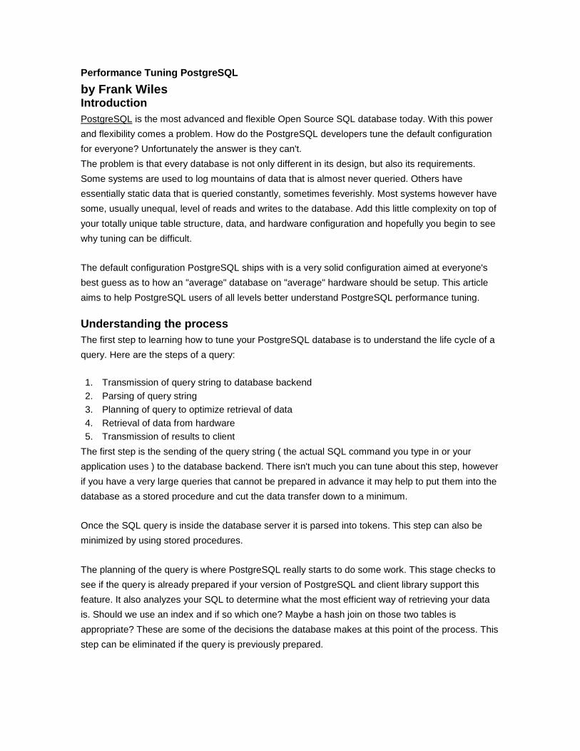
Performance Tuning PostgreSQL

by Frank Wiles Introduction

PostgreSQL is the most advanced and flexible Open Source SQL database today. With this power

and flexibility comes a problem. How do the PostgreSQL developers tune the default configuration

for everyone? Unfortunately the answer is they can't.

The problem is that every database is not only different in its design, but also its requirements.

Some systems are used to log mountains of data that is almost never queried. Others have

essentially static data that is queried constantly, sometimes feverishly. Most systems however have

some, usually unequal, level of reads and writes to the database. Add this little complexity on top of

your totally unique table structure, data, and hardware configuration and hopefully you begin to see

why tuning can be difficult.

The default configuration PostgreSQL ships with is a very solid configuration aimed at everyone's

best guess as to how an "average" database on "average" hardware should be setup. This article

aims to help PostgreSQL users of all levels better understand PostgreSQL performance tuning.

Understanding the process

The first step to learning how to tune your PostgreSQL database is to understand the life cycle of a

query. Here are the steps of a query:

1. Transmission of query string to database backend

2. Parsing of query string

3. Planning of query to optimize retrieval of data

4. Retrieval of data from hardware

5. Transmission of results to client

The first step is the sending of the query string ( the actual SQL command you type in or your

application uses ) to the database backend. There isn't much you can tune about this step, however

if you have a very large queries that cannot be prepared in advance it may help to put them into the

database as a stored procedure and cut the data transfer down to a minimum.

Once the SQL query is inside the database server it is parsed into tokens. This step can also be

minimized by using stored procedures.

The planning of the query is where PostgreSQL really starts to do some work. This stage checks to

see if the query is already prepared if your version of PostgreSQL and client library support this

feature. It also analyzes your SQL to determine what the most efficient way of retrieving your data

is. Should we use an index and if so which one? Maybe a hash join on those two tables is

appropriate? These are some of the decisions the database makes at this point of the process. This

step can be eliminated if the query is previously prepared.

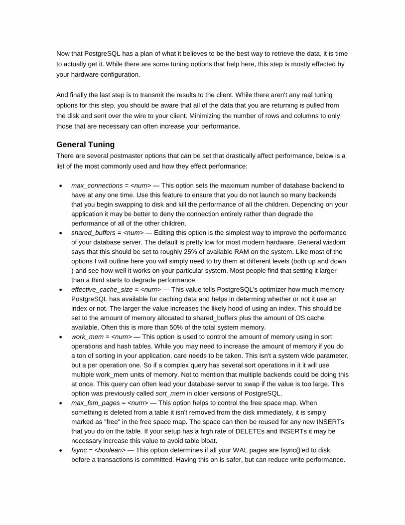
Now that PostgreSQL has a plan of what it believes to be the best way to retrieve the data, it is time

to actually get it. While there are some tuning options that help here, this step is mostly effected by

your hardware configuration.

And finally the last step is to transmit the results to the client. While there aren't any real tuning

options for this step, you should be aware that all of the data that you are returning is pulled from

the disk and sent over the wire to your client. Minimizing the number of rows and columns to only

those that are necessary can often increase your performance.

General Tuning

There are several postmaster options that can be set that drastically affect performance, below is a

list of the most commonly used and how they effect performance:

max_connections = <num> — This option sets the maximum number of database backend to

have at any one time. Use this feature to ensure that you do not launch so many backends

that you begin swapping to disk and kill the performance of all the children. Depending on your

application it may be better to deny the connection entirely rather than degrade the

performance of all of the other children.

shared_buffers = <num> — Editing this option is the simplest way to improve the performance

of your database server. The default is pretty low for most modern hardware. General wisdom

says that this should be set to roughly 25% of available RAM on the system. Like most of the

options I will outline here you will simply need to try them at different levels (both up and down

) and see how well it works on your particular system. Most people find that setting it larger

than a third starts to degrade performance.

effective_cache_size = <num> — This value tells PostgreSQL's optimizer how much memory

PostgreSQL has available for caching data and helps in determing whether or not it use an

index or not. The larger the value increases the likely hood of using an index. This should be

set to the amount of memory allocated to shared_buffers plus the amount of OS cache

available. Often this is more than 50% of the total system memory.

work_mem = <num> — This option is used to control the amount of memory using in sort

operations and hash tables. While you may need to increase the amount of memory if you do

a ton of sorting in your application, care needs to be taken. This isn't a system wide parameter,

but a per operation one. So if a complex query has several sort operations in it it will use

multiple work_mem units of memory. Not to mention that multiple backends could be doing this

at once. This query can often lead your database server to swap if the value is too large. This

option was previously called sort_mem in older versions of PostgreSQL.

max_fsm_pages = <num> — This option helps to control the free space map. When

something is deleted from a table it isn't removed from the disk immediately, it is simply

marked as "free" in the free space map. The space can then be reused for any new INSERTs

that you do on the table. If your setup has a high rate of DELETEs and INSERTs it may be

necessary increase this value to avoid table bloat.

fsync = <boolean> — This option determines if all your WAL pages are fsync()'ed to disk

before a transactions is committed. Having this on is safer, but can reduce write performance.

If fsync is not enabled there is the chance of unrecoverable data corruption. Turn this off at

your own risk.

commit_delay = <num> and commit_siblings = <num> — These options are used in concert to

help improve performance by writing out multiple transactions that are committing at once. If

there are commit_siblings number of backends active at the instant your transaction is

committing then the server waiting commit_delay microseconds to try and commit multiple

transactions at once.

random_page_cost = <num> — random_page_cost controls the way PostgreSQL views non-

sequential disk reads. A higher value makes it more likely that a sequential scan will be used

over an index scan indicating that your server has very fast disks.

If this is still confusing to you, Revolution Systems does offer aPostgreSQL Tuning Service

Note that many of these options consume shared memory and it will probably be necessary to

increase the amount of shared memory allowed on your system to get the most out of these

options.

Hardware Issues

Obviously the type and quality of the hardware you use for your database server drastically impacts

the performance of your database. Here are a few tips to use when purchasing hardware for your

database server (in order of importance):

RAM — The more RAM you have the more disk cache you will have. This greatly impacts

performance considering memory I/O is thousands of times faster than disk I/O.

Disk types — Obviously fast Ultra-320 SCSI disks are your best option, however high end

SATA drives are also very good. With SATA each disk is substantially cheaper and with that

you can afford more spindles than with SCSI on the same budget.

Disk configuration — The optimum configuration is RAID 1+0 with as many disks as possible

and with your transaction log (pg_xlog) on a separate disk ( or stripe ) all by itself. RAID 5 is

not a very good option for databases unless you have more than 6 disks in your volume. With

newer versions of PostgreSQL you can also use the tablespaces option to put different tables,

databases, and indexes on different disks to help optimize performance. Such as putting your

often used tables on a fast SCSI disk and the less used ones slower IDE or SATA drives.

CPUs — The more CPUs the better, however if your database does not use many complex

functions your money is best spent on more RAM or a better disk subsystem.

In general the more RAM and disk spindles you have in your system the better it will perform. This

is because with the extra RAM you will access your disks less. And the extra spindles help spread

the reads and writes over multiple disks to increase throughput and to reduce drive head

congestion.

Another good idea is to separate your application code and your database server onto different

hardware. Not only does this provide more hardware dedicated to the database server, but the

operating system's disk cache will contain more PostgreSQL data and not other various application

or system data this way.

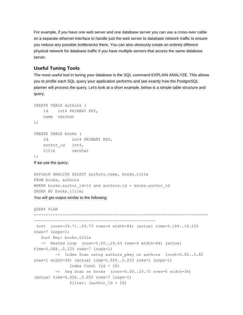
For example, if you have one web server and one database server you can use a cross-over cable

on a separate ethernet interface to handle just the web server to database network traffic to ensure

you reduce any possible bottlenecks there. You can also obviously create an entirely different

physical network for database traffic if you have multiple servers that access the same database

server.

Useful Tuning Tools

The most useful tool in tuning your database is the SQL command EXPLAIN ANALYZE. This allows

you to profile each SQL query your application performs and see exactly how the PostgreSQL

planner will process the query. Let's look at a short example, below is a simple table structure and

query.

CREATE TABLE authors (

id int4 PRIMARY KEY,

name varchar

);

CREATE TABLE books (

id int4 PRIMARY KEY,

author_id int4,

title varchar

);

If we use the query:

EXPLAIN ANALYZE SELECT authors.name, books.title

FROM books, authors

WHERE books.author_id=16 and authors.id = books.author_id

ORDER BY books.title;

You will get output similar to the following:

QUERY PLAN

-------------------------------------------------------------------------

---------------------------------------------------

Sort (cost=29.71..29.73 rows=6 width=64) (actual time=0.189..16.233

rows=7 loops=1)

Sort Key: books.title

-> Nested Loop (cost=0.00..29.63 rows=6 width=64) (actual

time=0.068..0.129 rows=7 loops=1)

-> Index Scan using authors_pkey on authors (cost=0.00..5.82

rows=1 width=36) (actual time=0.029..0.033 rows=1 loops=1)

Index Cond: (id = 16)

-> Seq Scan on books (cost=0.00..23.75 rows=6 width=36)

(actual time=0.026..0.052 rows=7 loops=1)

Filter: (author_id = 16)

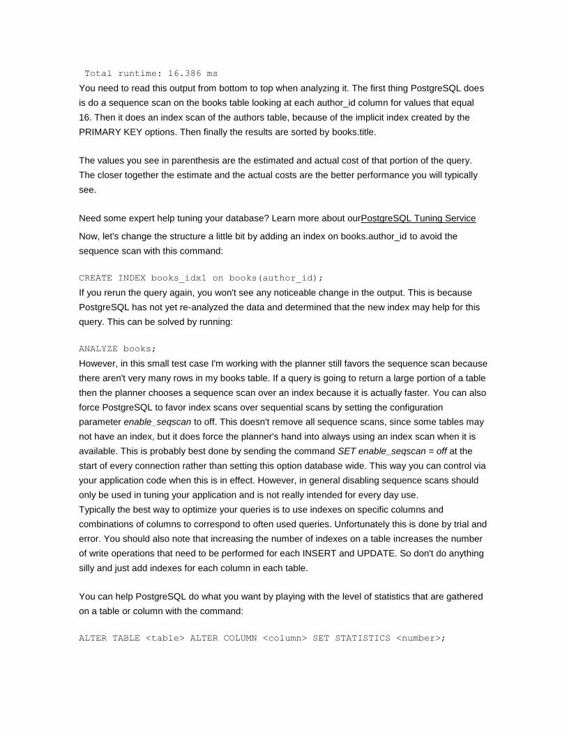
Total runtime: 16.386 ms

You need to read this output from bottom to top when analyzing it. The first thing PostgreSQL does

is do a sequence scan on the books table looking at each author_id column for values that equal

16. Then it does an index scan of the authors table, because of the implicit index created by the

PRIMARY KEY options. Then finally the results are sorted by books.title.

The values you see in parenthesis are the estimated and actual cost of that portion of the query.

The closer together the estimate and the actual costs are the better performance you will typically

see.

Need some expert help tuning your database? Learn more about ourPostgreSQL Tuning Service

Now, let's change the structure a little bit by adding an index on books.author_id to avoid the

sequence scan with this command:

CREATE INDEX books_idx1 on books(author_id);

If you rerun the query again, you won't see any noticeable change in the output. This is because

PostgreSQL has not yet re-analyzed the data and determined that the new index may help for this

query. This can be solved by running:

ANALYZE books;

However, in this small test case I'm working with the planner still favors the sequence scan because

there aren't very many rows in my books table. If a query is going to return a large portion of a table

then the planner chooses a sequence scan over an index because it is actually faster. You can also

force PostgreSQL to favor index scans over sequential scans by setting the configuration

parameter enable_seqscan to off. This doesn't remove all sequence scans, since some tables may

not have an index, but it does force the planner's hand into always using an index scan when it is

available. This is probably best done by sending the command SET enable_seqscan = off at the

start of every connection rather than setting this option database wide. This way you can control via

your application code when this is in effect. However, in general disabling sequence scans should

only be used in tuning your application and is not really intended for every day use.

Typically the best way to optimize your queries is to use indexes on specific columns and

combinations of columns to correspond to often used queries. Unfortunately this is done by trial and

error. You should also note that increasing the number of indexes on a table increases the number

of write operations that need to be performed for each INSERT and UPDATE. So don't do anything

silly and just add indexes for each column in each table.

You can help PostgreSQL do what you want by playing with the level of statistics that are gathered

on a table or column with the command:

ALTER TABLE <table> ALTER COLUMN <column> SET STATISTICS <number>;

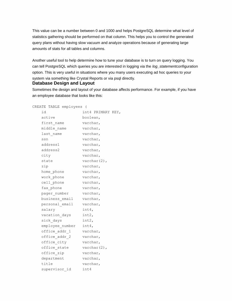
This value can be a number between 0 and 1000 and helps PostgreSQL determine what level of

statistics gathering should be performed on that column. This helps you to control the generated

query plans without having slow vacuum and analyze operations because of generating large

amounts of stats for all tables and columns.

Another useful tool to help determine how to tune your database is to turn on query logging. You

can tell PostgreSQL which queries you are interested in logging via the log_statementconfiguration

option. This is very useful in situations where you many users executing ad hoc queries to your

system via something like Crystal Reports or via psql directly.

Database Design and Layout

Sometimes the design and layout of your database affects performance. For example, if you have

an employee database that looks like this:

CREATE TABLE employees (

id int4 PRIMARY KEY,

active boolean,

first_name varchar,

middle_name varchar,

last_name varchar,

ssn varchar,

address1 varchar,

address2 varchar,

city varchar,

state varchar(2),

zip varchar,

home_phone varchar,

work_phone varchar,

cell_phone varchar,

fax_phone varchar,

pager_number varchar,

business_email varchar,

personal_email varchar,

salary int4,

vacation_days int2,

sick_days int2,

employee_number int4,

office_addr_1 varchar,

office_addr_2 varchar,

office_city varchar,

office_state varchar(2),

office_zip varchar,

department varchar,

title varchar,

supervisor_id int4

);

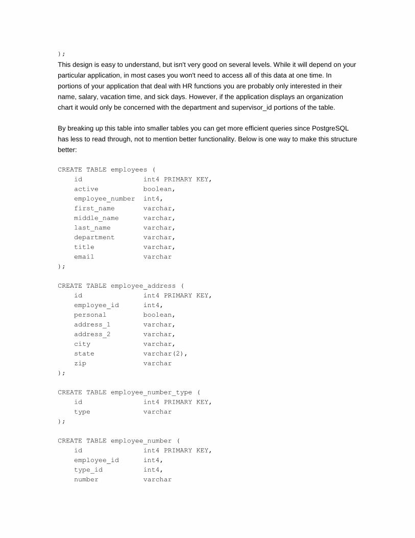
This design is easy to understand, but isn't very good on several levels. While it will depend on your

particular application, in most cases you won't need to access all of this data at one time. In

portions of your application that deal with HR functions you are probably only interested in their

name, salary, vacation time, and sick days. However, if the application displays an organization

chart it would only be concerned with the department and supervisor_id portions of the table.

By breaking up this table into smaller tables you can get more efficient queries since PostgreSQL

has less to read through, not to mention better functionality. Below is one way to make this structure

better:

CREATE TABLE employees (

id int4 PRIMARY KEY,

active boolean,

employee_number int4,

first_name varchar,

middle_name varchar,

last_name varchar,

department varchar,

title varchar,

email varchar

);

CREATE TABLE employee_address (

id int4 PRIMARY KEY,

employee_id int4,

personal boolean,

address_1 varchar,

address_2 varchar,

city varchar,

state varchar(2),

zip varchar

);

CREATE TABLE employee_number_type (

id int4 PRIMARY KEY,

type varchar

);

CREATE TABLE employee_number (

id int4 PRIMARY KEY,

employee_id int4,

type_id int4,

number varchar

);

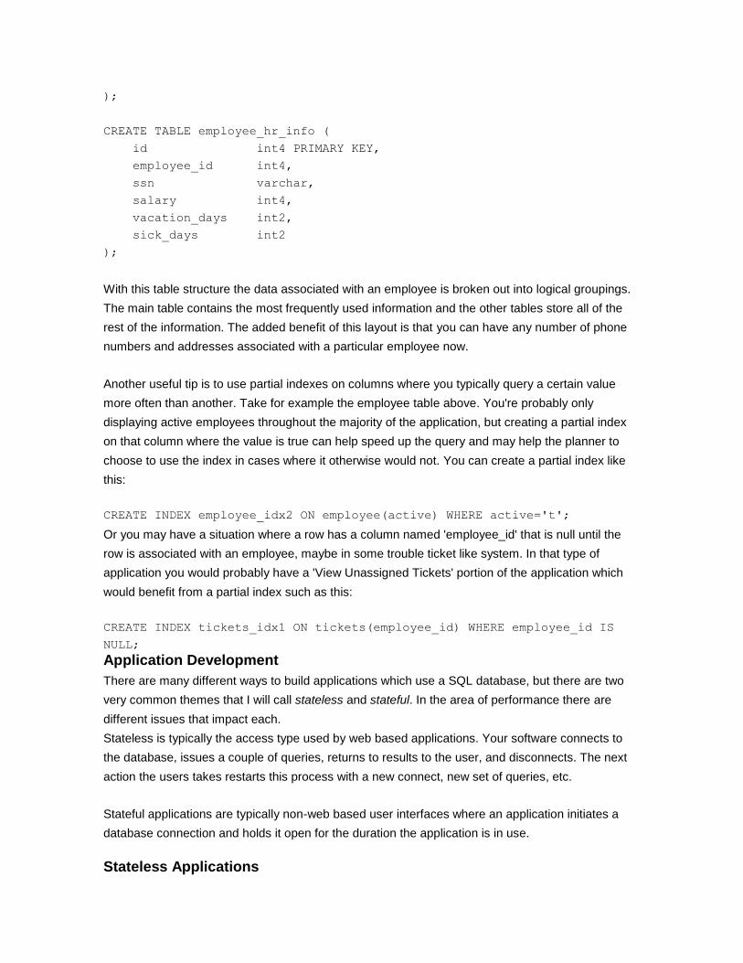
CREATE TABLE employee_hr_info (

id int4 PRIMARY KEY,

employee_id int4,

ssn varchar,

salary int4,

vacation_days int2,

sick_days int2

);

With this table structure the data associated with an employee is broken out into logical groupings.

The main table contains the most frequently used information and the other tables store all of the

rest of the information. The added benefit of this layout is that you can have any number of phone

numbers and addresses associated with a particular employee now.

Another useful tip is to use partial indexes on columns where you typically query a certain value

more often than another. Take for example the employee table above. You're probably only

displaying active employees throughout the majority of the application, but creating a partial index

on that column where the value is true can help speed up the query and may help the planner to

choose to use the index in cases where it otherwise would not. You can create a partial index like

this:

CREATE INDEX employee_idx2 ON employee(active) WHERE active='t';

Or you may have a situation where a row has a column named 'employee_id' that is null until the

row is associated with an employee, maybe in some trouble ticket like system. In that type of

application you would probably have a 'View Unassigned Tickets' portion of the application which

would benefit from a partial index such as this:

CREATE INDEX tickets_idx1 ON tickets(employee_id) WHERE employee_id IS

NULL;

Application Development

There are many different ways to build applications which use a SQL database, but there are two

very common themes that I will call stateless and stateful. In the area of performance there are

different issues that impact each.

Stateless is typically the access type used by web based applications. Your software connects to

the database, issues a couple of queries, returns to results to the user, and disconnects. The next

action the users takes restarts this process with a new connect, new set of queries, etc.

Stateful applications are typically non-web based user interfaces where an application initiates a

database connection and holds it open for the duration the application is in use.

Stateless Applications

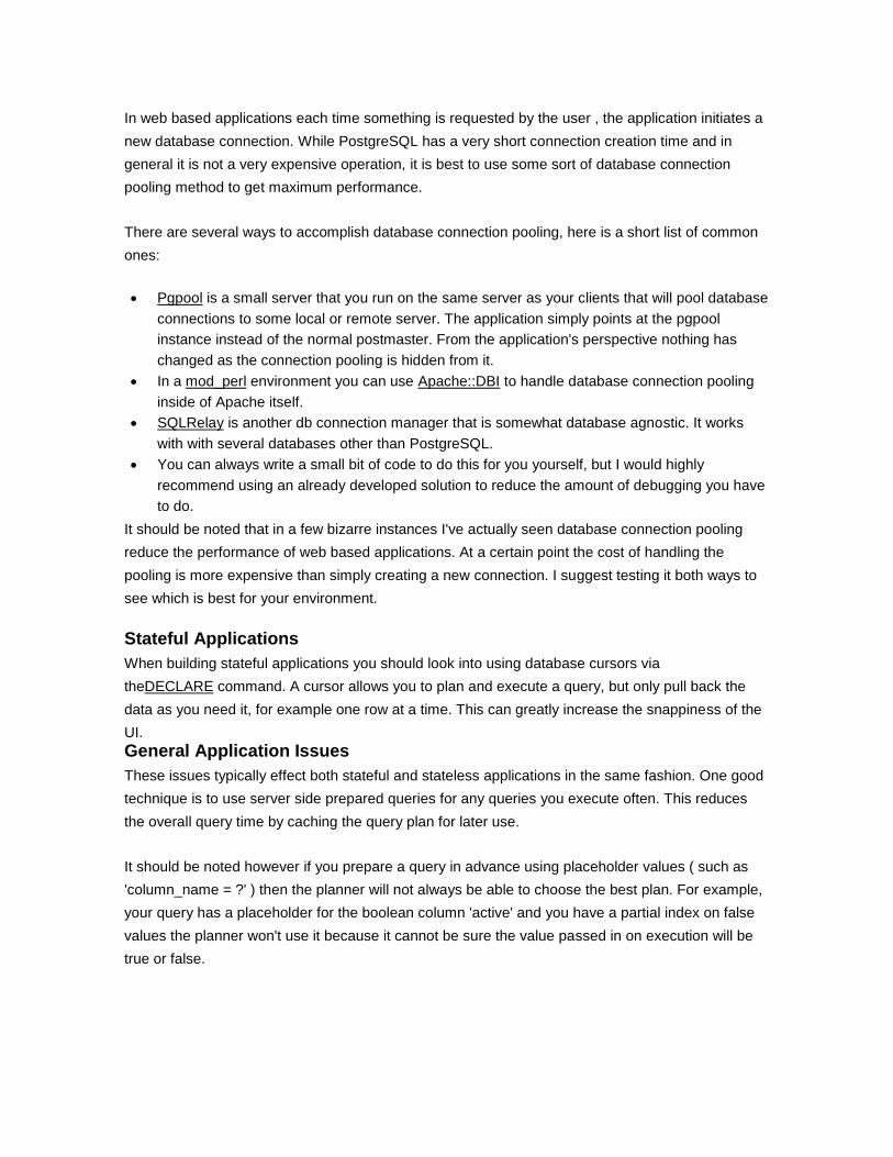
In web based applications each time something is requested by the user , the application initiates a

new database connection. While PostgreSQL has a very short connection creation time and in

general it is not a very expensive operation, it is best to use some sort of database connection

pooling method to get maximum performance.

There are several ways to accomplish database connection pooling, here is a short list of common

ones:

Pgpool is a small server that you run on the same server as your clients that will pool database

connections to some local or remote server. The application simply points at the pgpool

instance instead of the normal postmaster. From the application's perspective nothing has

changed as the connection pooling is hidden from it.

In a mod_perl environment you can use Apache::DBI to handle database connection pooling

inside of Apache itself.

SQLRelay is another db connection manager that is somewhat database agnostic. It works

with with several databases other than PostgreSQL.

You can always write a small bit of code to do this for you yourself, but I would highly

recommend using an already developed solution to reduce the amount of debugging you have

to do.

It should be noted that in a few bizarre instances I've actually seen database connection pooling

reduce the performance of web based applications. At a certain point the cost of handling the

pooling is more expensive than simply creating a new connection. I suggest testing it both ways to

see which is best for your environment.

Stateful Applications

When building stateful applications you should look into using database cursors via

theDECLARE command. A cursor allows you to plan and execute a query, but only pull back the

data as you need it, for example one row at a time. This can greatly increase the snappiness of the

UI.

General Application Issues

These issues typically effect both stateful and stateless applications in the same fashion. One good

technique is to use server side prepared queries for any queries you execute often. This reduces

the overall query time by caching the query plan for later use.

It should be noted however if you prepare a query in advance using placeholder values ( such as

'column_name = ?' ) then the planner will not always be able to choose the best plan. For example,

your query has a placeholder for the boolean column 'active' and you have a partial index on false

values the planner won't use it because it cannot be sure the value passed in on execution will be

true or false.

You can also obviously utilize stored procedures here to reduce the transmit, parse, and plan

portions of the typical query life cycle. It is best to profile your application and find commonly used

queries and data manipulations and put them into a stored procedure.

Tuning al rendimiento de PostgreSQL Publicado el 9 septiembre, 2011 por wiccano Publicado en Sin categoría 2 respuestas

Antes en entrar en el tema me parece importante aclarar el término anglosajón Tuning con el

que nos referimos a ―puesta a punto‖ de algo.

PostgreSQL es actualmente la Base de Datos SQL de código abierto más avanzada y flexible.

Con este poder y flexibilidad enfrentamos un problema: los desarrolladores de PostgreSQL

suelen ajustar la configuración de modo general, lamentablemente esto no se debe hacer. Esto

se hace para asegurar que el servidor arrancará casi con cualquier configuración hardware.

El punto esta en que cada base de datos no solo es diferente en su diseño sino también en sus

necesidades. Algunas por ejemplo, se usan para recopilar grandes cantidades de datos que casi

nunca son consultados y otras en cambio tienen datos estáticos y que son consultados

frecuentemente. Sin embargo la mayoría de sistemas tienen niveles de escritura y lectura sobre

la base de datos, generalmente desiguales. Sumando a esto la estructura total de la base de

datos, sus tipos de datos y configuración de hardware hacen que hacer tuning al rendimiento de

PostgreSQL no sea una tarea fácil.

Sitios de Referencia:

http://wiki.postgresql.org/wiki/Tuning_Your_PostgreSQL_Server

Entendiendo el proceso

El primer paso para entender como funciona una base de datos PostgreSQL es entender el ciclo

de vida de una consulta. Estos son los pasos que sigue una consulta:

1. Transmisión de la cadena de consulta al backend de la base de datos

2. Análisis(Parsing) de la cadena de consulta

3. Planificación de la consulta para optimizar la recuperación de datos

4. Recuperación de datos desde el hardware

5. Transmisión de los resultados del cliente

El primer paso es el envío de la cadena de consulta (el comando SQL que se tipea desde la

aplicación que se este usando) a la base de datos. No hay mucho que usted pueda ajustar en este

punto. Sin embargo si usted tiene consultas muy grandes o largas que no se construyen de

forma avanzada puede optar por ponerlas en la base de datos como procedimientos

almacenados y así cortar la transferencia de datos a un mínimo que vendría siendo el llamado al

procedimiento almacenado.

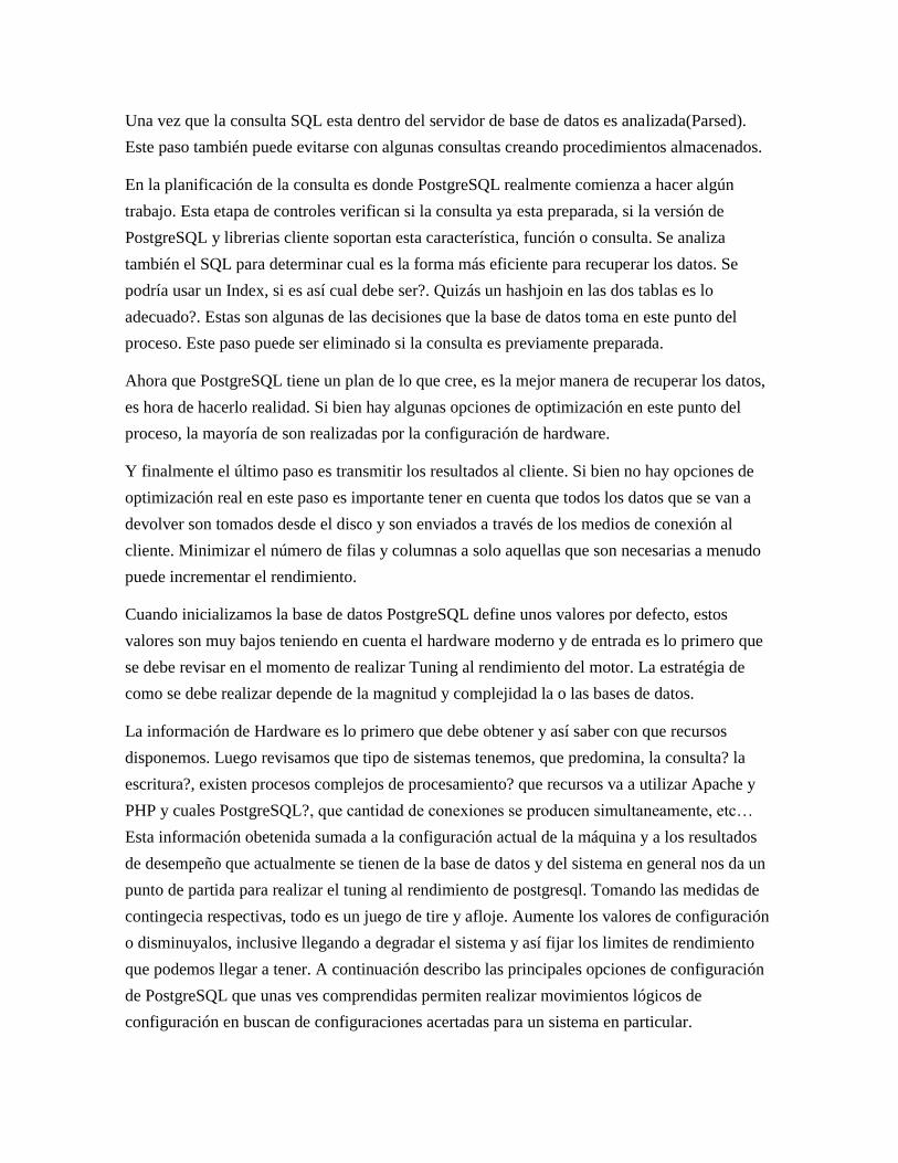
Una vez que la consulta SQL esta dentro del servidor de base de datos es analizada(Parsed).

Este paso también puede evitarse con algunas consultas creando procedimientos almacenados.

En la planificación de la consulta es donde PostgreSQL realmente comienza a hacer algún

trabajo. Esta etapa de controles verifican si la consulta ya esta preparada, si la versión de

PostgreSQL y librerias cliente soportan esta característica, función o consulta. Se analiza

también el SQL para determinar cual es la forma más eficiente para recuperar los datos. Se

podría usar un Index, si es así cual debe ser?. Quizás un hashjoin en las dos tablas es lo

adecuado?. Estas son algunas de las decisiones que la base de datos toma en este punto del

proceso. Este paso puede ser eliminado si la consulta es previamente preparada.

Ahora que PostgreSQL tiene un plan de lo que cree, es la mejor manera de recuperar los datos,

es hora de hacerlo realidad. Si bien hay algunas opciones de optimización en este punto del

proceso, la mayoría de son realizadas por la configuración de hardware.

Y finalmente el último paso es transmitir los resultados al cliente. Si bien no hay opciones de

optimización real en este paso es importante tener en cuenta que todos los datos que se van a

devolver son tomados desde el disco y son enviados a través de los medios de conexión al

cliente. Minimizar el número de filas y columnas a solo aquellas que son necesarias a menudo

puede incrementar el rendimiento.

Cuando inicializamos la base de datos PostgreSQL define unos valores por defecto, estos

valores son muy bajos teniendo en cuenta el hardware moderno y de entrada es lo primero que

se debe revisar en el momento de realizar Tuning al rendimiento del motor. La estratégia de

como se debe realizar depende de la magnitud y complejidad la o las bases de datos.

La información de Hardware es lo primero que debe obtener y así saber con que recursos

disponemos. Luego revisamos que tipo de sistemas tenemos, que predomina, la consulta? la

escritura?, existen procesos complejos de procesamiento? que recursos va a utilizar Apache y

PHP y cuales PostgreSQL?, que cantidad de conexiones se producen simultaneamente, etc…

Esta información obetenida sumada a la configuración actual de la máquina y a los resultados

de desempeño que actualmente se tienen de la base de datos y del sistema en general nos da un

punto de partida para realizar el tuning al rendimiento de postgresql. Tomando las medidas de

contingecia respectivas, todo es un juego de tire y afloje. Aumente los valores de configuración

o disminuyalos, inclusive llegando a degradar el sistema y así fijar los limites de rendimiento

que podemos llegar a tener. A continuación describo las principales opciones de configuración

de PostgreSQL que unas ves comprendidas permiten realizar movimientos lógicos de

configuración en buscan de configuraciones acertadas para un sistema en particular.

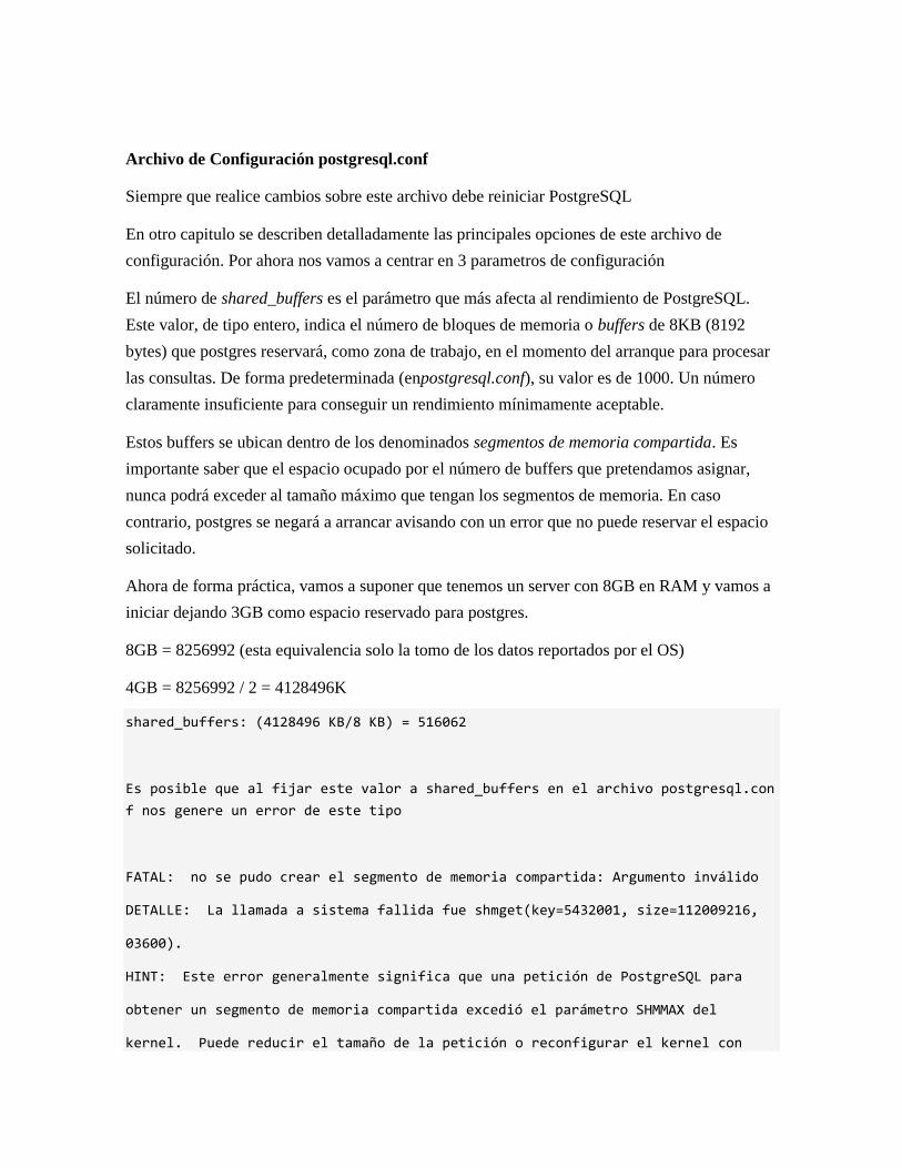
Archivo de Configuración postgresql.conf

Siempre que realice cambios sobre este archivo debe reiniciar PostgreSQL

En otro capitulo se describen detalladamente las principales opciones de este archivo de

configuración. Por ahora nos vamos a centrar en 3 parametros de configuración

El número de shared_buffers es el parámetro que más afecta al rendimiento de PostgreSQL.

Este valor, de tipo entero, indica el número de bloques de memoria o buffers de 8KB (8192

bytes) que postgres reservará, como zona de trabajo, en el momento del arranque para procesar

las consultas. De forma predeterminada (enpostgresql.conf), su valor es de 1000. Un número

claramente insuficiente para conseguir un rendimiento mínimamente aceptable.

Estos buffers se ubican dentro de los denominados segmentos de memoria compartida. Es

importante saber que el espacio ocupado por el número de buffers que pretendamos asignar,

nunca podrá exceder al tamaño máximo que tengan los segmentos de memoria. En caso

contrario, postgres se negará a arrancar avisando con un error que no puede reservar el espacio

solicitado.

Ahora de forma práctica, vamos a suponer que tenemos un server con 8GB en RAM y vamos a

iniciar dejando 3GB como espacio reservado para postgres.

8GB = 8256992 (esta equivalencia solo la tomo de los datos reportados por el OS)

4GB = 8256992 / 2 = 4128496K

shared_buffers: (4128496 KB/8 KB) = 516062

Es posible que al fijar este valor a shared_buffers en el archivo postgresql.con

f nos genere un error de este tipo

FATAL: no se pudo crear el segmento de memoria compartida: Argumento inválido

DETALLE: La llamada a sistema fallida fue shmget(key=5432001, size=112009216,

03600).

HINT: Este error generalmente significa que una petición de PostgreSQL para

obtener un segmento de memoria compartida excedió el parámetro SHMMAX del

kernel. Puede reducir el tamaño de la petición o reconfigurar el kernel con

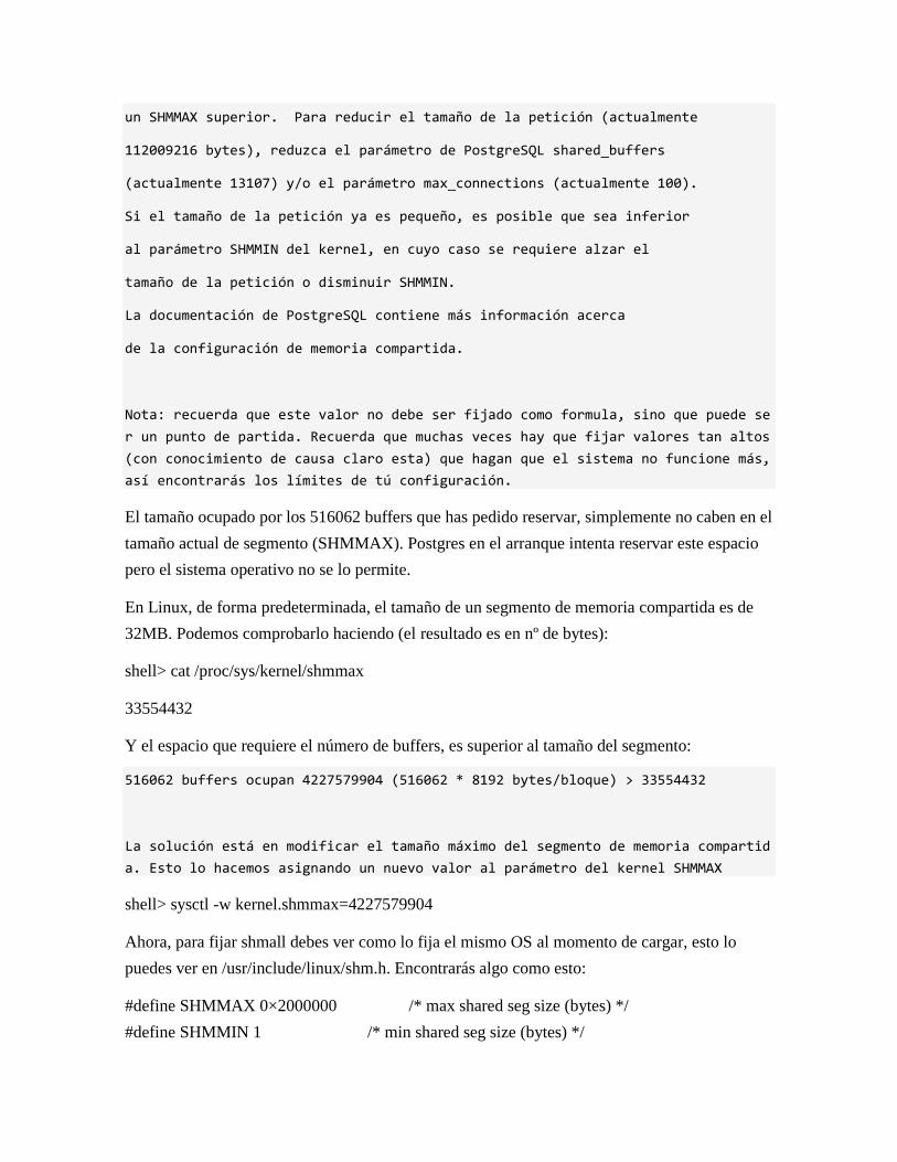
un SHMMAX superior. Para reducir el tamaño de la petición (actualmente

112009216 bytes), reduzca el parámetro de PostgreSQL shared_buffers

(actualmente 13107) y/o el parámetro max_connections (actualmente 100).

Si el tamaño de la petición ya es pequeño, es posible que sea inferior

al parámetro SHMMIN del kernel, en cuyo caso se requiere alzar el

tamaño de la petición o disminuir SHMMIN.

La documentación de PostgreSQL contiene más información acerca

de la configuración de memoria compartida.

Nota: recuerda que este valor no debe ser fijado como formula, sino que puede se

r un punto de partida. Recuerda que muchas veces hay que fijar valores tan altos

(con conocimiento de causa claro esta) que hagan que el sistema no funcione más,

así encontrarás los límites de tú configuración.

El tamaño ocupado por los 516062 buffers que has pedido reservar, simplemente no caben en el

tamaño actual de segmento (SHMMAX). Postgres en el arranque intenta reservar este espacio

pero el sistema operativo no se lo permite.

En Linux, de forma predeterminada, el tamaño de un segmento de memoria compartida es de

32MB. Podemos comprobarlo haciendo (el resultado es en nº de bytes):

shell> cat /proc/sys/kernel/shmmax

33554432

Y el espacio que requiere el número de buffers, es superior al tamaño del segmento:

516062 buffers ocupan 4227579904 (516062 * 8192 bytes/bloque) > 33554432

La solución está en modificar el tamaño máximo del segmento de memoria compartid

a. Esto lo hacemos asignando un nuevo valor al parámetro del kernel SHMMAX

shell> sysctl -w kernel.shmmax=4227579904

Ahora, para fijar shmall debes ver como lo fija el mismo OS al momento de cargar, esto lo

puedes ver en /usr/include/linux/shm.h. Encontrarás algo como esto:

#define SHMMAX 0×2000000 /* max shared seg size (bytes) */

#define SHMMIN 1 /* min shared seg size (bytes) */

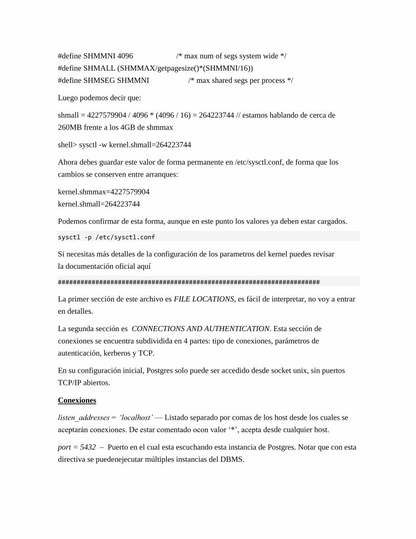
#define SHMMNI 4096 /* max num of segs system wide */

#define SHMALL (SHMMAX/getpagesize()*(SHMMNI/16))

#define SHMSEG SHMMNI /* max shared segs per process */

Luego podemos decir que:

shmall = 4227579904 / 4096 * (4096 / 16) = 264223744 // estamos hablando de cerca de

260MB frente a los 4GB de shmmax

shell> sysctl -w kernel.shmall=264223744

Ahora debes guardar este valor de forma permanente en /etc/sysctl.conf, de forma que los

cambios se conserven entre arranques:

kernel.shmmax=4227579904

kernel.shmall=264223744

Podemos confirmar de esta forma, aunque en este punto los valores ya deben estar cargados.

sysctl -p /etc/sysctl.conf

Si necesitas más detalles de la configuración de los parametros del kernel puedes revisar

la documentación oficial aquí

######################################################################

La primer sección de este archivo es FILE LOCATIONS, es fácil de interpretar, no voy a entrar

en detalles.

La segunda sección es CONNECTIONS AND AUTHENTICATION. Esta sección de

conexiones se encuentra subdividida en 4 partes: tipo de conexiones, parámetros de

autenticación, kerberos y TCP.

En su configuración inicial, Postgres solo puede ser accedido desde socket unix, sin puertos

TCP/IP abiertos.

Conexiones

listen_addresses = ‘localhost’ — Listado separado por comas de los host desde los cuales se

aceptarán conexiones. De estar comentado ocon valor ‗*‘, acepta desde cualquier host.

port = 5432 – Puerto en el cual esta escuchando esta instancia de Postgres. Notar que con esta

directiva se puedenejecutar múltiples instancias del DBMS.

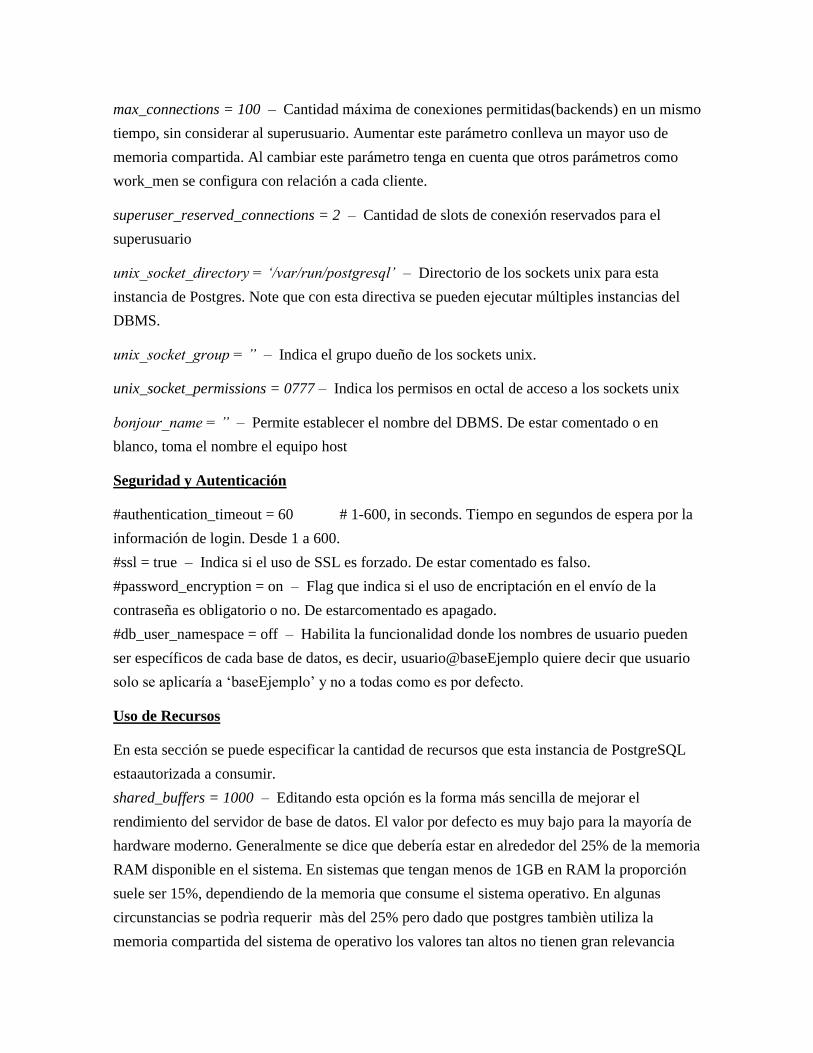
max_connections = 100 – Cantidad máxima de conexiones permitidas(backends) en un mismo

tiempo, sin considerar al superusuario. Aumentar este parámetro conlleva un mayor uso de

memoria compartida. Al cambiar este parámetro tenga en cuenta que otros parámetros como

work_men se configura con relación a cada cliente.

superuser_reserved_connections = 2 – Cantidad de slots de conexión reservados para el

superusuario

unix_socket_directory = ‘/var/run/postgresql’ – Directorio de los sockets unix para esta

instancia de Postgres. Note que con esta directiva se pueden ejecutar múltiples instancias del

DBMS.

unix_socket_group = ” – Indica el grupo dueño de los sockets unix.

unix_socket_permissions = 0777 – Indica los permisos en octal de acceso a los sockets unix

bonjour_name = ” – Permite establecer el nombre del DBMS. De estar comentado o en

blanco, toma el nombre el equipo host

Seguridad y Autenticación

#authentication_timeout = 60 # 1-600, in seconds. Tiempo en segundos de espera por la

información de login. Desde 1 a 600.

#ssl = true – Indica si el uso de SSL es forzado. De estar comentado es falso.

#password_encryption = on – Flag que indica si el uso de encriptación en el envío de la

contraseña es obligatorio o no. De estarcomentado es apagado.

#db_user_namespace = off – Habilita la funcionalidad donde los nombres de usuario pueden

ser específicos de cada base de datos, es decir, usuario@baseEjemplo quiere decir que usuario

solo se aplicaría a ‗baseEjemplo‘ y no a todas como es por defecto.

Uso de Recursos

En esta sección se puede especificar la cantidad de recursos que esta instancia de PostgreSQL

estaautorizada a consumir.

shared_buffers = 1000 – Editando esta opción es la forma más sencilla de mejorar el

rendimiento del servidor de base de datos. El valor por defecto es muy bajo para la mayoría de

hardware moderno. Generalmente se dice que debería estar en alrededor del 25% de la memoria

RAM disponible en el sistema. En sistemas que tengan menos de 1GB en RAM la proporción

suele ser 15%, dependiendo de la memoria que consume el sistema operativo. En algunas

circunstancias se podrìa requerir màs del 25% pero dado que postgres tambièn utiliza la

memoria compartida del sistema de operativo los valores tan altos no tienen gran relevancia

frente a los valores bajos. Tenga en cuenta que para sistemas abajo de la versión 8.1 los valores

altos en shared_buffers no funcionan bien, en cambio se pueden tener valores de 32MB a cerca

de 400MB funcionando correctamente.

Como la mayoría de las opciones que se resumen aquí, simplemente tendrá que probar

diferentes valores, hacia arriba y hacía abajo, y ver que tan bien funciona el sistema. Muchas

personas van fijando valores altos hasta encontrar el valor que degrada el sistema y así ir

encontrando el ideal.

temp_buffers = 1000 – Los buffers temporales hacen referencia a la cantidad de memoria

utilizada por cada sesión de base de datos para acceder a tablas temporales.

#max_prepared_transactions = 5 – Se recomienda dejar por defecto.5

work_mem = 1024 – Este valor se debe fijar con relación al parámetro max_connections, si

por ejemplo tiene 400 conexiones simultaneas y fija work_mem en 20MB estará utilizando

8GB de memoria compartida. Tenga en cuenta esta medida y fije el valor suficiente ya que este

le permite mejorar el rendimiento de consultas de ordenamiento complejo. Por ejmeplo.

maintenance_work_mem = 16384 – Esta directiva en kilobytes, indica la cantidad de memoria

a utilizar por las labores de mantención como VACUUM, CREATE INDEX, restauración de

bases de datos, etc. Como no se suelen dar operaciones concurrentes de este tipo dejarlo en un

valor como 256MB esta bien.

max_fsm_pages = 20000 – Esta opción ayuda a controlar el Mapeo de Espacio Libre (free

space map(FSM)). Cuando algo es eliminado de la tabla no es removido del disco

inmediatamente. El espacio es realmente marcado como libre en el FSM. El espacio puede ser

reutilizado para cualquier nuevo INSERT realizado en la tabla. Si el sistema tiene una alta tasa

de INSERT y DELETE puede ser necesario aumentar este valor para evitar que las tablas

aumenten desmesuradamente su tamaño.

max_fsm_relations = 1000 – Cantidad de relaciones (tablas e índices) de las cuales se

mantiene monitoreo del espacio libre en el mapade espacio libre. Deben ser al menos 100

Ajustes a las Consultas (Query Tuning)

Configuración de las funciones del planificador. Desabilite la función que necesite pasando a

off

#enable_bitmapscan = on

#enable_hashagg = on

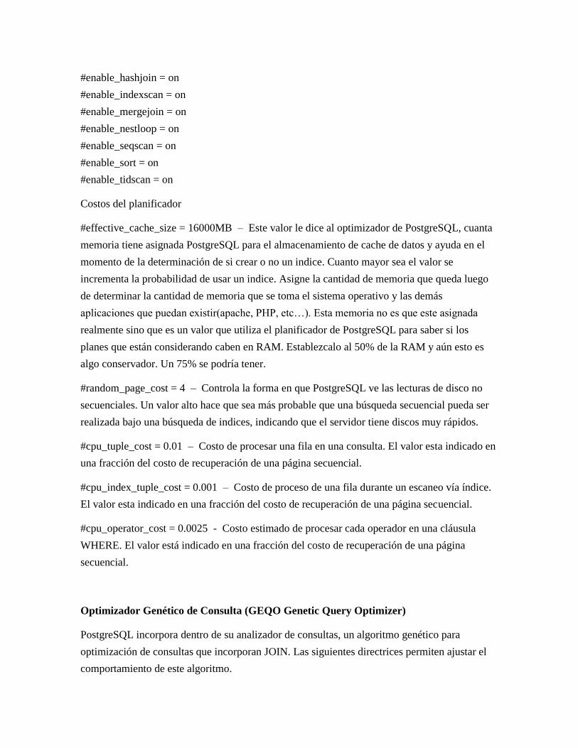
#enable_hashjoin = on

#enable_indexscan = on

#enable_mergejoin = on

#enable_nestloop = on

#enable_seqscan = on

#enable_sort = on

#enable_tidscan = on

Costos del planificador

#effective_cache_size = 16000MB – Este valor le dice al optimizador de PostgreSQL, cuanta

memoria tiene asignada PostgreSQL para el almacenamiento de cache de datos y ayuda en el

momento de la determinación de si crear o no un indice. Cuanto mayor sea el valor se

incrementa la probabilidad de usar un indice. Asigne la cantidad de memoria que queda luego

de determinar la cantidad de memoria que se toma el sistema operativo y las demás

aplicaciones que puedan existir(apache, PHP, etc…). Esta memoria no es que este asignada

realmente sino que es un valor que utiliza el planificador de PostgreSQL para saber si los

planes que están considerando caben en RAM. Establezcalo al 50% de la RAM y aún esto es

algo conservador. Un 75% se podría tener.

#random_page_cost = 4 – Controla la forma en que PostgreSQL ve las lecturas de disco no

secuenciales. Un valor alto hace que sea más probable que una búsqueda secuencial pueda ser

realizada bajo una búsqueda de indices, indicando que el servidor tiene discos muy rápidos.

#cpu_tuple_cost = 0.01 – Costo de procesar una fila en una consulta. El valor esta indicado en

una fracción del costo de recuperación de una página secuencial.

#cpu_index_tuple_cost = 0.001 – Costo de proceso de una fila durante un escaneo vía índice.

El valor esta indicado en una fracción del costo de recuperación de una página secuencial.

#cpu_operator_cost = 0.0025 - Costo estimado de procesar cada operador en una cláusula

WHERE. El valor está indicado en una fracción del costo de recuperación de una página

secuencial.

Optimizador Genético de Consulta (GEQO Genetic Query Optimizer)

PostgreSQL incorpora dentro de su analizador de consultas, un algoritmo genético para

optimización de consultas que incorporan JOIN. Las siguientes directrices permiten ajustar el

comportamiento de este algoritmo.

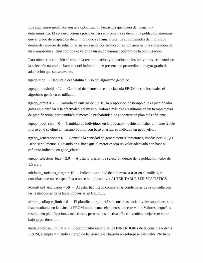
Los algoritmos genéticos son una optimización heurística que opera de forma no-

determinística. El set desoluciones posibles para el problema se denomina población, mientras

que el grado de adaptación de un individuo se llama ajuste. Las coordenadas del individuo

dentro del espacio de soluciones se representa por cromosomas. Un gene es una subsección de

un cromosoma el cual codifica el valor de un único parámetrodentro de la optimización.

Para obtener la solución se simula la recombinación y mutación de los individuos, realizándose

la selección natural en base a aquel individuo que presenta en promedio un mayor grado de

adaptación que sus ancestros.

#geqo = on – Habilita o deshabilita el uso del algorítmo genético.

#geqo_threshold = 12 – Cantidad de elementos en la cláusula FROM desde los cuales el

algorítmo genético es utilizado.

#geqo_effort 0 5 – Controla en enteros de 1 a 10, la proporción de tiempo que el planificador

gasta en planificar y la efectivdad del mismo. Valores más altos resultarán en un tiempo mayor

de planificación, pero también aumenta la probabilidad de encontrar un plan más eficiente.

#geqo_pool_size = 0 – Cantidad de individuos en la población, debiendo haber al menos 2. De

fijarse en 0 se elige un tamaño óptimo con base al esfuerzo indicado en geqo_effort

#geqo_generations = 0 – Controla la cantidad de generaciones(iteraciones) usadas por GEQO.

Debe ser al menos 1. Fijando en 0 hace que el motor escoja un valor adecuado con base al

esfuerzo indicado en geqo_effort.

#geqo_selection_bias = 2.0 – Ajusta la presión de selección dentro de la población, valor de

1.5 a 2.0.

#default_statistics_target = 10 – Indica la cantidad de columnas a usar en el análisis, en

consultas que no se especifica o no se ha indicado vía ALTER TABLE SER STATISTICS.

#constraint_exclusion = off – Al estar habilitado compara las condiciones de la consulta con

las restricciones de la tabla impuestas en CHECK.

#from _collapse_limit = 8 – El planificador juntará subconsultas hacia niveles superiores si la

lista resultante en la cláusula FROM notiene más elementos que este valor. Valores pequeños

resultan en planificaciones más cortas, pero menosefectivas. Es conveniente dejar este valor

bajo gego_threshold.

#join_collapse_limit = 8 – El planificador rescribirá los INNER JOINs de la consulta a items

FROM, siempre y cuando el largo de la listaen esa cláusula no sobrepase este valor. No tiene

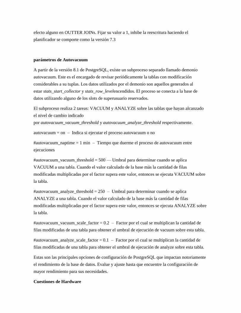
efecto alguno en OUTTER JOINs. Fijar su valor a 1, inhibe la reescritura haciendo el

planificador se comporte como la versión 7.3

parámetros de Autovacuum

A partir de la versión 8.1 de PostgreSQL, existe un subproceso separado llamado demonio

autovacuum. Este es el encargado de revisar periódicamente la tablas con modificación

considerables a su tuplas. Los datos utilizados por el demonio son aquellos generados al

estar stats_start_collector y stats_row_levelencendidos. El proceso se conecta a la base de

datos utilizando alguno de los slots de superusuario reservados.

El subproceso realiza 2 tareas: VACUUM y ANALYZE sobre las tablas que hayan alcanzado

el nivel de cambio indicado

por autovacuum_vacuum_threshold y autovacuum_analyze_threshold respectivamente.

autovacuum = on – Indica si ejecutar el proceso autovacuum o no

#autovacuum_naptime = 1 min – Tiempo que duerme el proceso de autovacuum entre

ejecuciones

#autovacuum_vacuum_threshold = 500 — Umbral para determinar cuando se aplica

VACUUM a una tabla. Cuando el valor calculado de la base más la cantidad de filas

modificadas multiplicadas por el factor supera este valor, entonces se ejecuta VACUUM sobre

la tabla.

#autovacuum_analyze_threshold = 250 – Umbral para determinar cuando se aplica

ANALYZE a una tabla. Cuando el valor calculado de la base más la cantidad de filas

modificadas multiplicadas por el factor supera este valor, entonces se ejecuta ANALYZE sobre

la tabla.

#autovacuum_vacuum_scale_factor = 0.2 – Factor por el cual se multiplican la cantidad de

filas modificadas de una tabla para obtener el umbral de ejecución de vacuum sobre esta tabla.

#autovacuum_analyze_scale_factor = 0.1 – Factor por el cual se multiplican la cantidad de

filas modificadas de una tabla para obtener el umbral de ejecución de analyze sobre esta tabla.

Estas son las principales opciones de configuración de PostgreSQL que impactan notoriamente

el rendimiento de la base de datos. Evalue y ajuste hasta que encuentre la configuración de

mayor rendimiento para sus necesidades.

Cuestiones de Hardware

Obviamente el tipo y la calidad de Hardware que se usa impacta drasticamente el rendimiento

de la base de datos. Estos son algunos consejos a la hora de comprar hardware para su servidor

de base de datos, en orden de importancia:

RAM — Entre más RAM se tenga debe tener más cache de disco. Esto afecta en gran medida el

rendimiento teniendo en cuenta que la memoria de E / S es miles de veces más rápida que la E / S del

disco.

Disk types — Definitivamente los rápidos discos SCSI Ultra-320 son la mejor opción. Sin embargo

los discos SATA de alta gama también son muy buenas. Los discos SATA son mucho más

económicos y con ellos se pueden tener muchos más ejes en su estructura de almacenamiento por el

mismo precio.

Disk configuration — La confuguración más óptima es RAID 1+0 con tantos discos como sea

posible y con le registro de transacciones (pg_xlog) en un disco independiente, bien sea físico o

viertual(Stripe Disk). RAID 5 no es una opción recomendada a no ser que tenga más de 6 discos en

su volumen. Con las nuevas versiones de PostgreSQL se puede utilizar la opción de tablespace para

poner tablas, base de datos e indices en discos diferentes para mejorar el dendimiento. Así como

poner las tablas de uso frecuente en un disco SCSI y las menos utilizadas en discos más lentos SATA

o IDE.

CPUs — Entre mejor CPU se tenga mejor rendimiento, sin embargo, si su base de datos no utiliza

muchas funciones complejas es mejor invertir el dinero en más memoria RAM o un mejor sistema de

discos.

En general cuanto más RAM se tenga y más posibilidad de conexiones de disco el sistema

funcionará mejor. Esto por que entre más RAM exista menos acceso al disco se realiza y entre

más conexiones de disco existan disponibles es posible distribuir las operaciones de lectura y

escritura en disco, aumentando el rendimiento y disminuyendo los cuellos de botella.

Otra buena idea es separar el código de la aplicación de la base de datos en diferente hardware.

Esto significa que no solo se va a tener más hardware disponible para la base de datos sino que

la memoria cache del sistema operativo contendrá más datos PostgreSQL y no de otro tipo de

aplicaciones o procesos.

Por ejemplo, si usted tiene un servidor web y un servidor de base de datos se puede usar un

cable cruzado por interfaces de redes exclusivas para que estos dos se comuniquen y a su vez el

servidor web utiliza otra conexión diferente para comunicarse con sus clientes. Si son varios

servidores web accediendo a un mismo servidor de base de datos podría armar una red

independiente y esclusiva para este tráfico.

Una vez tengamos la mejor configuración es ideal revisar todo tipo de consultas que recibe la

base de datos y ver en que medida se puede mejorar su rendimiento. Para iniciar debe ubicar las

consultas más repetitivas y las que más consumen tiempo de ejecución. En otro articulo puede

encontrar más información de como ubicar este tipo de consultas.

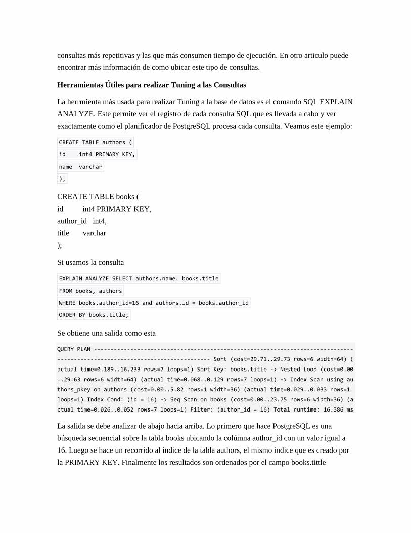
Herramientas Útiles para realizar Tuning a las Consultas

La herrmienta más usada para realizar Tuning a la base de datos es el comando SQL EXPLAIN

ANALYZE. Este permite ver el registro de cada consulta SQL que es llevada a cabo y ver

exactamente como el planificador de PostgreSQL procesa cada consulta. Veamos este ejemplo:

CREATE TABLE authors (

id int4 PRIMARY KEY,

name varchar

);

CREATE TABLE books (

id int4 PRIMARY KEY,

author_id int4,

title varchar

);

Si usamos la consulta

EXPLAIN ANALYZE SELECT authors.name, books.title

FROM books, authors

WHERE books.author_id=16 and authors.id = books.author_id

ORDER BY books.title;

Se obtiene una salida como esta

QUERY PLAN ------------------------------------------------------------------------------

---------------------------------------------- Sort (cost=29.71..29.73 rows=6 width=64) (

actual time=0.189..16.233 rows=7 loops=1) Sort Key: books.title -> Nested Loop (cost=0.00

..29.63 rows=6 width=64) (actual time=0.068..0.129 rows=7 loops=1) -> Index Scan using au

thors_pkey on authors (cost=0.00..5.82 rows=1 width=36) (actual time=0.029..0.033 rows=1

loops=1) Index Cond: (id = 16) -> Seq Scan on books (cost=0.00..23.75 rows=6 width=36) (a

ctual time=0.026..0.052 rows=7 loops=1) Filter: (author_id = 16) Total runtime: 16.386 ms

La salida se debe analizar de abajo hacia arriba. Lo primero que hace PostgreSQL es una

búsqueda secuencial sobre la tabla books ubicando la colúmna author_id con un valor igual a

16. Luego se hace un recorrido al indice de la tabla authors, el mismo indice que es creado por

la PRIMARY KEY. Finalmente los resultados son ordenados por el campo books.tittle

Los valores que se ven en paréntesis son el costo estimado y actual de esa parte de la consulta.

Cuanto menor sea la diferencia entre estos dos valores existeme un mejor desempeño.

Ahora vamos a cambiar un poco la estructura con la adición de un Index en books.author_id y

así evitar la búsqueda secuencial.

CREATE INDEX books_idx1 on books(author_id);

Si se vuelve a ejecutar la consulta de nuevo usted no vera ningún cambio notable en la salida.

Estos es por que PostgreSQL no ha vuelto a analizar los datos y no ha determinado que el

nuevo index puede ayudar en la consulta. Esto se puede solucionar mediante la ejecución de:

ANALYZE books;

Puede que no note cambios en los resultados de la búsqueda en secuencia si la tabla no contiene

muchos registros. Si una consulta va a retornar una gran cantidad de datos, el planificador

selecciona una búsqueda en secuencia a través del indice, ya que es más rápido. Se puede forzar

PosgreSQL a favor de las búsquedas por indices sobre las búsquedas secuenciales fijando el

parámetro de configuración enable_seqscan = off . Esto no quita todas las búsquedas por

secuencia ya que algunas tablas pueden no tener indices pero si fuerza al planificador a utilizar

siempre una búsqueda por indices cuando estos estén disponibles y sin importar si la cantidad

de datos a retornar es mínima. Es recomendable hacer este cambio en la parte inicial de cada

conexión con a la base de datos, por medio del comando SET enable_seqscan = off , y no

hacerlo ampliamente en todas las bases de datos. Sin embargo desactivas esta opción se hace en

casos de pruebas y de realización de Tuning y no como opción de uso diario.

Generalmente la mejor forma de optimizar las consultas es usar indices en colúmnas específicas

y combinaciones de colúmnas que corresponden a las consultas más frecuentes.

Lamentablemente esto se hace por ensayo y error. También debe tener en cuenta que

incrementar el número de indices en una tabla incrementa el número de operaciones de

escritura que se deben realizar para cada INSERT y UPDATE. Así que no haga cosas tontas

como agregar indices a todas las colúmnas de una tabla.

Algo que puede ayudar es jugar con el nivel de las estadísticas que se recogen en una tabla o

columna con el comando:

ALTER TABLE <table> ALTER COLUMN <column> SET STATISTICS <number>;

Este valor puede ser un número entre 0 y 1000 y ayuda a PostgreSQL a determinar el nivel de

recopilación de estadísticas que se debe realizar en esta columna. Esto ayuda a controlar la

generación del plan de la consulta sin tener VACUUM lentos y analizar las operaciones debido

a la generación de grandes cantidades de estadísticas para todas las tablas y columnas.

Otra herramienta útil para ayudar a determinar como hacer Tuning a la base de datos son las

consultas al registro del sistema. Se puede decir a PostgreSQL que consultas del registro nos

interesan a través de la opción de configuración de log_statement. Esto es muy útil en

situaciones donde hay muchos usuarios realizando consultas tipo ad hoc() en el sistema a través

de algo como Crystal Reports o directamente vía PSQL.

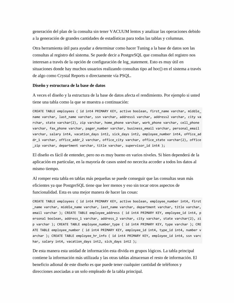
Diseño y estructura de la base de datos

A veces el diseño y la estructura de la base de datos afecta el rendimiento. Por ejemplo si usted

tiene una tabla como la que se muestra a continuación:

CREATE TABLE employees ( id int4 PRIMARY KEY, active boolean, first_name varchar, middle_

name varchar, last_name varchar, ssn varchar, address1 varchar, address2 varchar, city va

rchar, state varchar(2), zip varchar, home_phone varchar, work_phone varchar, cell_phone

varchar, fax_phone varchar, pager_number varchar, business_email varchar, personal_email

varchar, salary int4, vacation_days int2, sick_days int2, employee_number int4, office_ad

dr_1 varchar, office_addr_2 varchar, office_city varchar, office_state varchar(2), office

_zip varchar, department varchar, title varchar, supervisor_id int4 );

El diseño es fácil de entender, pero no es muy bueno en varios niveles. Si bien dependerá de la

aplicación en particular, en la mayoría de casos usted no nececita acceder a todos los datos al

mismo tiempo.

Al romper esta tabla en tablas más pequeñas se puede conseguir que las consultas sean más

eficientes ya que PostgreSQL tiene que leer menos y eso sin tocar otros aspectos de

funcionalidad. Esta es una mejor manera de hacer las cosas:

CREATE TABLE employees ( id int4 PRIMARY KEY, active boolean, employee_number int4, first

_name varchar, middle_name varchar, last_name varchar, department varchar, title varchar,

email varchar ); CREATE TABLE employee_address ( id int4 PRIMARY KEY, employee_id int4, p

ersonal boolean, address_1 varchar, address_2 varchar, city varchar, state varchar(2), zi

p varchar ); CREATE TABLE employee_number_type ( id int4 PRIMARY KEY, type varchar ); CRE

ATE TABLE employee_number ( id int4 PRIMARY KEY, employee_id int4, type_id int4, number v

archar ); CREATE TABLE employee_hr_info ( id int4 PRIMARY KEY, employee_id int4, ssn varc

har, salary int4, vacation_days int2, sick_days int2 );

De esta manera esta unidad de información esta divida en grupos lógicos. La tabla principal

contiene la información más utilizada y las otras tablas almacenan el resto de información. El

beneficio adional de este diseño es que puede tener cualquier cantidad de teléfonos y

direcciones asociadas a un solo empleado de la tabla principal.

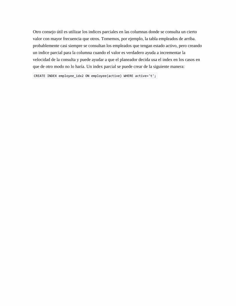
Otro consejo útil es utilizar los indices parciales en las columnas donde se consulta un cierto

valor con mayor frecuencia que otros. Tomemos, por ejemplo, la tabla empleados de arriba.

probablemente casi siempre se consultan los empleados que tengan estado activo, pero creando

un indice parcial para la columna cuando el valor es verdadero ayuda a incrementar la

velocidad de la consulta y puede ayudar a que el planeador decida usa el index en los casos en

que de otro modo no lo haría. Un index parcial se puede crear de la siguiente manera:

CREATE INDEX employee_idx2 ON employee(active) WHERE active='t';