Air Force Institute of TechnologyAFIT Scholar

Theses and Dissertations Student Graduate Works

3-24-2016

Performance Testing of Various Nozzle Design forWater Electrolysis ThrusterYuen Liu

Follow this and additional works at: https://scholar.afit.edu/etd

Part of the Propulsion and Power Commons

This Thesis is brought to you for free and open access by the Student Graduate Works at AFIT Scholar. It has been accepted for inclusion in Theses andDissertations by an authorized administrator of AFIT Scholar. For more information, please contact richard.mansfield@afit.edu.

Recommended CitationLiu, Yuen, "Performance Testing of Various Nozzle Design for Water Electrolysis Thruster" (2016). Theses and Dissertations. 437.https://scholar.afit.edu/etd/437

Performance Testing of Various Nozzle Designsfor Water Electrolysis Thruster

THESIS

Yuen Jing Monica Liu, Second Lieutenant, USAF

AFIT-ENY-MS-16-M-225

DEPARTMENT OF THE AIR FORCEAIR UNIVERSITY

AIR FORCE INSTITUTE OF TECHNOLOGY

Wright-Patterson Air Force Base, Ohio

DISTRIBUTION STATEMENT AAPPROVED FOR PUBLIC RELEASE; DISTRIBUTION UNLIMITED.

The views expressed in this document are those of the author and do not reflect theofficial policy or position of the United States Air Force, the United States Departmentof Defense or the United States Government. This material is declared a work of theU.S. Government and is not subject to copyright protection in the United States.

AFIT-ENY-MS-16-M-225

PERFORMANCE TESTING OF VARIOUS NOZZLE DESIGNS FOR WATER

ELECTROLYSIS THRUSTER

THESIS

Presented to the Faculty

Department of Astronautical Engineering

Graduate School of Engineering and Management

Air Force Institute of Technology

Air University

Air Education and Training Command

in Partial Fulfillment of the Requirements for the

Degree of Master of Science in Astronautical Engineering

Yuen Jing Monica Liu, B.S.A.E.

Second Lieutenant, USAF

March 3, 2016

DISTRIBUTION STATEMENT AAPPROVED FOR PUBLIC RELEASE; DISTRIBUTION UNLIMITED.

AFIT-ENY-MS-16-M-225

PERFORMANCE TESTING OF VARIOUS NOZZLE DESIGNS FOR WATER

ELECTROLYSIS THRUSTER

THESIS

Yuen Jing Monica Liu, B.S.A.E.Second Lieutenant, USAF

Committee Membership:

Dr. Carl Hartsfield, PhDChair

Dr. David Liu, PhDMember

Dr. Bill Hargus, PhDMember

AFIT-ENY-MS-16-M-225

Abstract

The purpose of this research is to develop new nozzles for the HYDROSTM thruster,

a pulsed chemical thruster, to improve the current flight performance. This research

consists of a base line test of the factory nozzle, as well as testing of three 15-

degree conical nozzles with different expansion ratios. Experiments were conducted

at plenum pressures 30, 40, and 45 psia to ensure the thruster is throttleable. Im-

pulse bit data was collected through measuring the impulse response of each firing

using a torsional balance thrust stand. Analysis of the thruster performance included

calculations of impulse bit, specific impulse, thrust coefficient, and exhaust plume at-

tachment. High speed images were taken to evaluate improvements in exhaust plume

attachment relative to nozzle contour. Experimental data showed that the smaller

expansion ratio nozzles have a higher performance than the larger expansion ratio

nozzles. This agrees with previous research from NASA that the benefit from the in-

crease in area ratio does not overcome the increased viscous losses due to the increase

in surface area for small throat areas. High speed images showed that the 15-degree

conical nozzle design helped improve the original nozzle’s flow separation problem.

Experimental results were also compared to ideal calculations from chemical equilib-

rium codes, and previous low Reynolds number nozzle research to evaluate loss in

thrust coefficient.

iv

Acknowledgements

I would like to thank my sponsor, Space Vehicles Directorate at Air Force

Research Lab, Kirkland AFB, for sponsoring this research. I would like to thank

Tethers Unlimited, Inc. for their troubleshooting assistance and for lending me their

thrust stand. Without this thrust stand, this research would not have been possible.

I also want to thank the technicians at AFIT machine shop for manufacturing the

three beautiful nozzles in a timely manner. In addition, I would like to express my

gratitude toward my research advisors, Major David Liu and Dr. Carl Hartsfield, for

their guidance, energy, and efforts in advising me throughout my research. I would

also like to thank my committee member, Dr. Bill Hargus, for his support as well.

Most importantly, I would like to thank my mother for working 12 hrs a day everyday,

for moving the family across the world, and for given up everything to allow me to

follow my dream. She taught me the importance in education and with that, this

research and masters degree is for her.

Yuen Jing Monica Liu

v

Table of Contents

Page

Abstract . . . . . . . . . . . . . . . . . . . . . . . . . . . . . . . . . . . . . . . . . . . . . . . . . . . . . . . . . . . . . . . iv

Acknowledgements . . . . . . . . . . . . . . . . . . . . . . . . . . . . . . . . . . . . . . . . . . . . . . . . . . . . . . . v

List of Figures . . . . . . . . . . . . . . . . . . . . . . . . . . . . . . . . . . . . . . . . . . . . . . . . . . . . . . . . . viii

List of Tables . . . . . . . . . . . . . . . . . . . . . . . . . . . . . . . . . . . . . . . . . . . . . . . . . . . . . . . . . . . xi

Symbol . . . . . . . . . . . . . . . . . . . . . . . . . . . . . . . . . . . . . . . . . . . . . . . . . . . . . . . . . . . . . . . xii

List of Abbreviations . . . . . . . . . . . . . . . . . . . . . . . . . . . . . . . . . . . . . . . . . . . . . . . . . . . xiv

I. Introduction . . . . . . . . . . . . . . . . . . . . . . . . . . . . . . . . . . . . . . . . . . . . . . . . . . . . . . . . 1

1.1 Background . . . . . . . . . . . . . . . . . . . . . . . . . . . . . . . . . . . . . . . . . . . . . . . . . . . . 11.2 Motivation . . . . . . . . . . . . . . . . . . . . . . . . . . . . . . . . . . . . . . . . . . . . . . . . . . . . . 31.3 Research Scope . . . . . . . . . . . . . . . . . . . . . . . . . . . . . . . . . . . . . . . . . . . . . . . . . 51.4 Research Objectives . . . . . . . . . . . . . . . . . . . . . . . . . . . . . . . . . . . . . . . . . . . . . 61.5 Assumptions and Limitations . . . . . . . . . . . . . . . . . . . . . . . . . . . . . . . . . . . . . 7

II. Literature Review . . . . . . . . . . . . . . . . . . . . . . . . . . . . . . . . . . . . . . . . . . . . . . . . . . . 8

2.1 Chemical Propulsion Systems Size Scaling . . . . . . . . . . . . . . . . . . . . . . . . . . 82.2 Nozzle Design . . . . . . . . . . . . . . . . . . . . . . . . . . . . . . . . . . . . . . . . . . . . . . . . . . 142.3 Low Reynolds Number Nozzle Performance . . . . . . . . . . . . . . . . . . . . . . . . 242.4 Water electrolysis systems and process . . . . . . . . . . . . . . . . . . . . . . . . . . . . 282.5 Hydrogen-Oxygen Combustion . . . . . . . . . . . . . . . . . . . . . . . . . . . . . . . . . . . 32

III. Test Methodology and Procedures . . . . . . . . . . . . . . . . . . . . . . . . . . . . . . . . . . . . 39

3.1 Introduction . . . . . . . . . . . . . . . . . . . . . . . . . . . . . . . . . . . . . . . . . . . . . . . . . . . 393.2 Equipment and Connections . . . . . . . . . . . . . . . . . . . . . . . . . . . . . . . . . . . . . 39

3.2.1 Vacuum Chamber . . . . . . . . . . . . . . . . . . . . . . . . . . . . . . . . . . . . . . . . 393.2.2 Torsional Balance Thrust Stand . . . . . . . . . . . . . . . . . . . . . . . . . . . . 413.2.3 Thruster . . . . . . . . . . . . . . . . . . . . . . . . . . . . . . . . . . . . . . . . . . . . . . . . 443.2.4 Equipment set-up . . . . . . . . . . . . . . . . . . . . . . . . . . . . . . . . . . . . . . . . 46

3.3 Calibration of Torsional Balance Thrust Stand . . . . . . . . . . . . . . . . . . . . . 503.4 Theoretical Calculations . . . . . . . . . . . . . . . . . . . . . . . . . . . . . . . . . . . . . . . . 563.5 Nozzle Designs . . . . . . . . . . . . . . . . . . . . . . . . . . . . . . . . . . . . . . . . . . . . . . . . . 623.6 Error analysis . . . . . . . . . . . . . . . . . . . . . . . . . . . . . . . . . . . . . . . . . . . . . . . . . . 66

vi

Page

IV. Results and Analysis . . . . . . . . . . . . . . . . . . . . . . . . . . . . . . . . . . . . . . . . . . . . . . . . 68

4.1 Thrust Stand Calibration Results . . . . . . . . . . . . . . . . . . . . . . . . . . . . . . . . 684.2 Performance Analysis . . . . . . . . . . . . . . . . . . . . . . . . . . . . . . . . . . . . . . . . . . . 72

4.2.1 Impulse Bit . . . . . . . . . . . . . . . . . . . . . . . . . . . . . . . . . . . . . . . . . . . . . 734.2.2 Specific Impulse . . . . . . . . . . . . . . . . . . . . . . . . . . . . . . . . . . . . . . . . . 774.2.3 Thrust Coefficient . . . . . . . . . . . . . . . . . . . . . . . . . . . . . . . . . . . . . . . . 88

4.3 Exhaust Plume Attachments . . . . . . . . . . . . . . . . . . . . . . . . . . . . . . . . . . . . . 93

V. Conclusions and Future Work . . . . . . . . . . . . . . . . . . . . . . . . . . . . . . . . . . . . . . . . 97

5.1 Research Objectives Review . . . . . . . . . . . . . . . . . . . . . . . . . . . . . . . . . . . . . 975.2 Recommendation and Future work . . . . . . . . . . . . . . . . . . . . . . . . . . . . . . . 100

5.2.1 Torsional Balance Thrust Stand . . . . . . . . . . . . . . . . . . . . . . . . . . . 1005.2.2 The water electrolysis thruster . . . . . . . . . . . . . . . . . . . . . . . . . . . . 101

Appendix A. Impulse Bit Data . . . . . . . . . . . . . . . . . . . . . . . . . . . . . . . . . . . . . . . . . . 103

Appendix B. Specific Impulse and Thrust Coefficient Data . . . . . . . . . . . . . . . . . . 108

Appendix C. Mass Per Fire Data . . . . . . . . . . . . . . . . . . . . . . . . . . . . . . . . . . . . . . . . 109

Bibliography . . . . . . . . . . . . . . . . . . . . . . . . . . . . . . . . . . . . . . . . . . . . . . . . . . . . . . . . . . 111

vii

List of Figures

Figure Page

1 High speed images of exhaust plume [14]. . . . . . . . . . . . . . . . . . . . . . . . . . . . 5

2 Thrust coefficient as a function of pressure ratio, nozzlearea ratio, and specific heat ratio [28]. . . . . . . . . . . . . . . . . . . . . . . . . . . . . 17

3 Exhaust plume pattern for different conditions [20]. . . . . . . . . . . . . . . . . . 18

4 Contour of a conical nozzle [6]. . . . . . . . . . . . . . . . . . . . . . . . . . . . . . . . . . . . 19

5 Nozzle contour of an ideal nozzle [20]. . . . . . . . . . . . . . . . . . . . . . . . . . . . . . 21

6 Nozzle contour of a bell nozzle [6]. . . . . . . . . . . . . . . . . . . . . . . . . . . . . . . . . 22

7 Nozzle contour of a parabolic bell nozzle [6]. . . . . . . . . . . . . . . . . . . . . . . . . 23

8 The relationship between nozzle area ratio and thrustcoefficient with a divergence angle of 20 degrees [26]. . . . . . . . . . . . . . . . . 27

9 Schematic Diagram of Electrolysis Cell [27]. . . . . . . . . . . . . . . . . . . . . . . . . 29

10 The electrolysis process [27]. . . . . . . . . . . . . . . . . . . . . . . . . . . . . . . . . . . . . . 30

11 Explosion limits of a stoichiometric hydrogen-oxygenmixture [13] . . . . . . . . . . . . . . . . . . . . . . . . . . . . . . . . . . . . . . . . . . . . . . . . . . . . 35

12 Space simulator vacuum system. . . . . . . . . . . . . . . . . . . . . . . . . . . . . . . . . . . 40

13 Vacuum to lab connections. . . . . . . . . . . . . . . . . . . . . . . . . . . . . . . . . . . . . . . 40

14 The window and passthrough location. . . . . . . . . . . . . . . . . . . . . . . . . . . . . 41

15 Rotational balance thrust stand with thruster. . . . . . . . . . . . . . . . . . . . . . . 42

16 Calibration hammer and motor. . . . . . . . . . . . . . . . . . . . . . . . . . . . . . . . . . . 43

17 LDS and micro-adjuster. . . . . . . . . . . . . . . . . . . . . . . . . . . . . . . . . . . . . . . . . . 44

18 Thruster stand and thruster inside the vacuum chamber. . . . . . . . . . . . . . 44

19 The HYDROSTM thruster used for this research. . . . . . . . . . . . . . . . . . . . . 45

20 The HYDROSTM thruster interface GUI used for thisresearch. . . . . . . . . . . . . . . . . . . . . . . . . . . . . . . . . . . . . . . . . . . . . . . . . . . . . . . . 46

viii

Figure Page

21 The lab side set-up. . . . . . . . . . . . . . . . . . . . . . . . . . . . . . . . . . . . . . . . . . . . . . 47

22 The complete experiment set-up. . . . . . . . . . . . . . . . . . . . . . . . . . . . . . . . . . 48

23 Swinging arm with LDS. . . . . . . . . . . . . . . . . . . . . . . . . . . . . . . . . . . . . . . . . 49

24 The camera set-up. . . . . . . . . . . . . . . . . . . . . . . . . . . . . . . . . . . . . . . . . . . . . . 50

25 The top view of the thrust stand. . . . . . . . . . . . . . . . . . . . . . . . . . . . . . . . . 51

26 Hammer impulse response. . . . . . . . . . . . . . . . . . . . . . . . . . . . . . . . . . . . . . . . 52

27 Impulse repsonse with key points. . . . . . . . . . . . . . . . . . . . . . . . . . . . . . . . . . 53

28 The measured response and the new response with theoriginal amplitude. . . . . . . . . . . . . . . . . . . . . . . . . . . . . . . . . . . . . . . . . . . . . . . 54

29 An impulse input from the hammer. . . . . . . . . . . . . . . . . . . . . . . . . . . . . . . . 55

30 An example of a hammer unit response. . . . . . . . . . . . . . . . . . . . . . . . . . . . 56

31 Loss in thrust coefficient due to viscous effects [26]. . . . . . . . . . . . . . . . . . . 61

32 Thrust coefficient vs. expansion ratio for differentReynolds numbers [26]. . . . . . . . . . . . . . . . . . . . . . . . . . . . . . . . . . . . . . . . . . . 61

33 CAD model of the factory nozzle . . . . . . . . . . . . . . . . . . . . . . . . . . . . . . . . . 62

34 Nozzle contour of the conical nozzle [6]. . . . . . . . . . . . . . . . . . . . . . . . . . . . . 63

35 CAD and manufactured model for nozzle 1. . . . . . . . . . . . . . . . . . . . . . . . 64

36 CAD and manufactured model for nozzle 2. . . . . . . . . . . . . . . . . . . . . . . . . 65

37 CAD and manufactured model for nozzle 3. . . . . . . . . . . . . . . . . . . . . . . . . 65

38 Nozzles comparison of the 4 nozzles [15]. . . . . . . . . . . . . . . . . . . . . . . . . . . . 66

39 The damping ratios of the thrust stand. . . . . . . . . . . . . . . . . . . . . . . . . . . . 69

40 The natural frequencies of the thrust stand. . . . . . . . . . . . . . . . . . . . . . . . . 70

41 Unit impulse responses magnitude of the thrust stand. . . . . . . . . . . . . . . . 70

42 Impulse bit data of the four nozzles. . . . . . . . . . . . . . . . . . . . . . . . . . . . . . . . 73

ix

Figure Page

43 Specific impulse data for all four nozzles in variousplenum pressures. . . . . . . . . . . . . . . . . . . . . . . . . . . . . . . . . . . . . . . . . . . . . . . . 78

44 The comparison between the experimental average massvalues and the ideal gas law mass values. . . . . . . . . . . . . . . . . . . . . . . . . . . . 81

45 New Isp data with updated mass values. . . . . . . . . . . . . . . . . . . . . . . . . . . . 81

46 Characteristics velocity values in CEA. . . . . . . . . . . . . . . . . . . . . . . . . . . . . 84

47 Loss percentage in specific impulse and thrustcoefficient based on Spisz et al. . . . . . . . . . . . . . . . . . . . . . . . . . . . . . . . . . . . 85

48 Loss percentage in performance between the expectedvalues and the measured values. . . . . . . . . . . . . . . . . . . . . . . . . . . . . . . . . . . 86

49 Overall loss percentage in performance between theideal values and the measured values. . . . . . . . . . . . . . . . . . . . . . . . . . . . . . . 87

50 The thrust coefficient data of the four nozzles at variousplenum pressure. . . . . . . . . . . . . . . . . . . . . . . . . . . . . . . . . . . . . . . . . . . . . . . . 88

51 The updated thrust coefficient data with massadjustment. . . . . . . . . . . . . . . . . . . . . . . . . . . . . . . . . . . . . . . . . . . . . . . . . . . . . 89

52 Thrust coefficient trend comparison with Spisz et al.research data. . . . . . . . . . . . . . . . . . . . . . . . . . . . . . . . . . . . . . . . . . . . . . . . . . . 92

53 High speed images of factory nozzle: Exposure time of264 ms (30 fps) [14]. . . . . . . . . . . . . . . . . . . . . . . . . . . . . . . . . . . . . . . . . . . . . 94

54 High speed images of Nozzle 1: Exposure time of 32 ms(125 fps). . . . . . . . . . . . . . . . . . . . . . . . . . . . . . . . . . . . . . . . . . . . . . . . . . . . . . . 95

55 High speed images of Nozzle 2: Exposure time of 32 ms(125 fps). . . . . . . . . . . . . . . . . . . . . . . . . . . . . . . . . . . . . . . . . . . . . . . . . . . . . . . 96

56 High speed images of Nozzle 3: Exposure time of 4 ms(500 fps). . . . . . . . . . . . . . . . . . . . . . . . . . . . . . . . . . . . . . . . . . . . . . . . . . . . . . . 96

x

List of Tables

Table Page

1 Optimal Nozzle Conditions . . . . . . . . . . . . . . . . . . . . . . . . . . . . . . . . . . . . . . 60

2 Optimal conditions for the three nozzle designs. . . . . . . . . . . . . . . . . . . . . . 66

3 A summary of expansion ratios. . . . . . . . . . . . . . . . . . . . . . . . . . . . . . . . . . . 66

4 Test conditions for the HYDROSTM thruster. . . . . . . . . . . . . . . . . . . . . . . . 72

5 The estimated throat conditions. . . . . . . . . . . . . . . . . . . . . . . . . . . . . . . . . . . 75

6 The average mass per fire for various plenum pressures. . . . . . . . . . . . . . . 79

7 Isp (sec) data comparison between the measured valuesand the expected values. . . . . . . . . . . . . . . . . . . . . . . . . . . . . . . . . . . . . . . . . . 83

8 Thrust coefficent comparison between measured andexpected thrust coefficient. . . . . . . . . . . . . . . . . . . . . . . . . . . . . . . . . . . . . . . . 90

9 Original Nozzle Raw Data (V) . . . . . . . . . . . . . . . . . . . . . . . . . . . . . . . . . . . 104

10 Nozzle 1 Raw Data (V) . . . . . . . . . . . . . . . . . . . . . . . . . . . . . . . . . . . . . . . . . 105

11 Nozzle 2 Raw Data (V) . . . . . . . . . . . . . . . . . . . . . . . . . . . . . . . . . . . . . . . . . 106

12 Nozzle 3 Raw Data (V) . . . . . . . . . . . . . . . . . . . . . . . . . . . . . . . . . . . . . . . . . 107

13 Isp data for the four nozzles. . . . . . . . . . . . . . . . . . . . . . . . . . . . . . . . . . . . . 108

14 Mass data for each test set. . . . . . . . . . . . . . . . . . . . . . . . . . . . . . . . . . . . . 110

xi

List of Symbols

CF Thrust coefficient

Pc Chamber pressure

At Throat area

Po Stagnation pressure

dt Throat diameter

Re Reynolds number

T Thrust

ρ Density

µ Dynamic viscosity

To Stagnation temperature

Da Damkoehler number

Cp Specific heat

P2 Exit pressure

ve Exit velocity

Ln Nozzle length

rt Throat radius

α Cone half angle

λ Correction factor

ε Expansion ratio

Rn Circular contour arc radius

m Mass flow rate (kg/s)

Isp Specific impulse (s)

Ibit Impulse bit (N-s)

A Amplitude

xii

ξ Damping ratio

ωn Natural frequency (rad)

µ Dynamic viscosity

M2 Exit mach number

T1 Chamber temperature (k)

k Specific heat ratio

R Specific gas constant

V2 Exit velocity (m/s)

SE Standard error

σ Error

m Average mass per fire

δm Change of mass per test set

c∗ Characteristics velocity

xiii

List of Abbreviations

TUI Tethers Unlimited, Inc.

CDH Command and Data Handling

NASA National Aeronautics and Space Administration

EPS Electrical power subsystem

AFIT Air Force Institute of Technology

MEMS Micro-Electro-Mechanical Systems

MOC Method of characteristics

TIC Truncated ideal contoured nozzle

SPE Solid Polymer Electrolyte

WFB Water feed barrier

LDS Linear displacement sensor

DAQ Data acquisition device

CEA Chemical Equilibrium with Applications

EMI Electromagnetic interference

xiv

PERFORMANCE TESTING OF VARIOUS NOZZLE DESIGNS FOR WATER

ELECTROLYSIS THRUSTER

I. Introduction

1.1 Background

Space missions are usually driven toward increased capability by more ambitious

and diverse objectives. These objectives drive spacecraft design and increase the

demand on subsystems, spacecraft size, mass, and complexity of ground control, which

ultimately increases the total cost. Funding has become a limitation on some major

scientific missions and opportunities for space exploration [2]. For these reasons,

over the past several decades, the demand for micro-satellites, such as CubeSats,

has increased due to growing interests for high-performance and low-cost satellites.

Advances in microelectronics make packaging the minimum functions in a smaller box

practical. These growing interests are expressed in the NASA slogan “better, faster,

and cheaper”. Reduction in life-cycle costs and incorporation of innovative technology

have become two of the primary goals for NASA missions [19]. Some advanced space

missions require microspacecraft to have a total wet mass as low as a few kilograms

[2]. Such missions include precise positioning and spacecraft constellations control for

interferometry missions, which aim to detect gravity waves and cosmic-rays, as well

as search for planets around distant solar systems [19].

CubeSats are sized in terms of blocks; one block is 1U, nominally a 10 cm x 10

cm x 10 cm cube. CubeSats currently in orbit range from 3U to 12U. The design

and volumetric constraints make it difficult to integrate propulsion systems on-board.

1

Propulsion systems need to work with other subsystems in the CubeSat, such as ther-

mal, electrical power subsystem (EPS), command and data handling (C&DH), and

payload. Depending on the propulsion power requirement, solar panel deployment is

sometimes needed to accommodation the thruster. Also, depending on the mission

and CubeSat systems requirements on-board, sometimes trade-offs between subsys-

tems are necessary to allow CubeSats to function. For example, in order to meet the

peak power limit, the payload might need to switch to “off”, while the propulsion

system is firing. The electromagnetic interference (EMI) from the thruster might

also mandate shutting the payload off, regardless of power considerations. Due to

these difficulties in design, as well as the severe mass, volume, and power constraints,

only a few CubeSats have been launched with a propulsion system [17]. In addition,

the selection of suitable propulsion hardware with the right size and mass for small

spacecraft is limited.

The HYDROSTM thruster is an electrolysis propulsion system developed by Teth-

ers Unlimited, Inc (TUI). It is specifically designed to fit in a 1U configuration, making

it a viable propulsion system for CubeSats. The idea of using liquid water as fuel

for spacecraft is not new. It was first developed through Stechman and Campbell

in 1973 [27]. However, using the water electrolysis process for micropropulsion is a

recent concept. The HYDROSTM thruster, developed by TUI, uses deionized water

as a propellant. Through the electrolysis process, the deionized water is electrolyzed

to produce hydrogen and oxygen gas. The gaseous hydrogen and oxygen are directed

into a gas storage tank before going through the injector and combustion chamber;

the mixtures create water vapor through combustion. This propulsion system is throt-

tleable through adjustable tank pressures up to 45 psi. The system requires up to 15

watts of power from the CubeSat EPS. The thruster operates similarly to a payload,

receiving data from a ground station to control the C&DH board. The C&DH board

2

runs the thruster interface board, which sends and receives signals from the thruster.

Based on the testing data provided by TUI, hydrogen gas is produced at a rate up to

4 sccm/W from a prototype fuel cell operating up to 88% efficiency. [34]

1.2 Motivation

Successful CubeSat programs can expand opportunities for space exploration. Re-

duced mass leads to reduced mission costs, allowing more missions to occur. Launch

cost, often constituting about 30% of the total mission cost, is largely driven by

spacecraft mass. Therefore, reducing mass can help reduce mission cost significantly

and a significant part of the remaining costs are driven by the high launch costs

[17]. By employing CubeSats to replace big satellites, it could better use the Depart-

ment of Defense’s budget. However, missions for propulsionless CubeSats are limited

and are thus far confined to low Earth orbit. Most CubeSats lack a propulsion sys-

tem—limiting the capability, such as lifetime and maneuvers, and mission profile. By

conducting research on CubeSat propulsion, more advanced CubeSat missions are

enabled.

Microspacecraft can enable a class of scientific and exploration missions which

require many simultaneous measurements displaced in position; as on a planet, a

small body, or in a region of space [8]. Micro propulsion systems have been developed

to improve CubeSat mission lifetime and increase their controllability over the orbit

once deployed. With propulsion systems on board, CubeSats can take on higher level

missions and integrate into future constellations. In addition, off-loading scientific

instruments from a large, single spacecraft onto a fleet of microspacecraft can reduce

mission risk. Losing a few microspacecraft may not jeopardize the entire mission and

they are cheap to replace compared to big satellites.

Propulsion systems for CubeSats must be efficient, simple, and scalable, based

3

on mission requirements. Research on the HYDROSTM thruster is beneficial for

CubeSat propulsion development because, unlike many other propulsion systems, this

thruster uses a storable, safe, odorless, and non-toxic propellant—water. Fuels such as

hydrazine require operators to wear protective suits during handling and use portable

propellant service carts to load and unload, which is far from ideal [29]. CubeSats are

commonly launched as secondary payloads on carrier rockets and, therefore, the space

industry regulates CubeSats to store chemical energy during launch on the order of

100 Watt-Hours and pressure vessels to 1.2 atm to protect the primary payloads from

system malfunctions [12]. Protection of the primary payload is one of the limiting

factors for propulsion systems in CubeSats. In addition, the HYDROSTM thrusters

fuel tank is scalable depending on the mission needs. Conducting research on the

HYDROSTM propulsion system can determine the capabilities and Information such

as firing rate, specific impulse, and thrust can help determine the amount of delta V

this thruster can generate for a given CubeSat mass.

In the Summer of 2014, atmospheric and vacuum testing of the thruster was

conducted at the Air Force Institute of Technology (AFIT) to verify system perfor-

mance. Images, shown in Figure 1, captured from a high-speed camera show the

exhaust plume was not attached to the nozzle in the vacuum chamber, thus decreas-

ing efficiency. This research will investigate and attempt to provide a solution to

this problem by integrating new nozzle designs. New nozzle development and testing

can help provide a better understanding of improvements in thrust and efficiency for

the various designs. In addition, most research on nozzle designs have been for fully-

developed, steady state flow. Unfortunately, depending on the chamber pressure, size,

and pulsed operation, flow in some micro-propulsion systems is not fully developed.

This research can bring an understanding to nozzle design and flow attachment for a

short (less than 0.5 sec) duration flow. With the completion of this research, future

4

Figure 1. High speed images of exhaust plume [14].

space operators can assess the advantages and disadvantages of various nozzle designs

for chemical micro-propulsion and their use on micro-satellites.

1.3 Research Scope

The purpose of this research is to develop new nozzles for the HYDROSTM thruster

in order to improve the current performance. This research consists of a baseline test

of the factory nozzle, as well as testing three additional nozzles with different char-

acteristics. Experiments are conducted with different plenum pressures to ensure the

thruster is throttleable. Thrust data are collected through the impulse bit measure-

5

ment of each firing using a torsional balance thrust stand. Analysis of the thruster

performance includes calculations of impulse bit, specific impulse, and thrust coeffi-

cient. A high-speed camera is used to compare the flow attachment for each nozzle.

Experimental results of all four nozzles will show how the nozzle length and expansion

ratio affect thrust performance for a short-duration flow.

1.4 Research Objectives

CubeSat missions are limited without a propulsion system. By integrating a

propulsion system, orbital maneuvers, orbit controls, station keeping, and formation

flying are feasible. CubeSats with propulsion systems can help reduce mission costs,

which can help the Air Force operate efficiently in a budget-constrained environment.

Investigating new nozzle designs can potentially increase the efficiency, the perfor-

mance of the HYDROSTM thruster, and increase mission capabilities. The goal for

this research is to understand how different nozzle contours affect performance and

efficiency in small pulsed chemical thrusters.

1. Design nozzles using a nominal two-dimensional conical nozzle geometry to

improve the specific impulse of the thruster and verify results by using the

experimental impulse bit data to calculate specific impulse.

2. For each nozzle design, experimentally measure performance criteria such as

impulse bits, thrust coefficient as a function of the plenum pressure envelope at

30, 40, and 45 psia, in vacuum using a torsional balance thrust stand.

3. Determine nozzle performance in various plenum pressure and expansion ratio

by comparing thrust coefficient.

4. Examine viscous effects on nozzles by comparing experimental data with ideal

CEA data and previous research data.

6

5. Determine nozzle efficiency improvement by comparing the exhaust flow attach-

ment points relative to the nozzle using images from a high-speed camera.

1.5 Assumptions and Limitations

This research is set up only to measure the impulse bits of the thruster. Therefore,

it is not possible to fully understand the state of the thruster and the combustion

process without knowing other properties. This experiment assumes the gaseous

hydrogen and oxygen are going through a stoichimetric reaction. The combustion

process is best estimated through Chemical Equilibrium with Applications (CEA). It

is assumed, based on that simulation, the combustion temperature is approximately

3208 K, and the computer code is a fair presentation of a real-life scenario. Due to

the small scale of the thruster, it is also reasonable to assume the flow is operating in

a low Reynolds number range, around 1800, which is calculated based on the CEA

ideal data. The system probably does not have complete combustion or a fully devel-

oped flow due to the small combustion chamber and pulsed operation. Due to time,

schedule, and resource constraints, some limitations include the number of nozzles

available for testing and experimental measurements. Experimental measurements

are limited to impulse bits only with no pressure or temperature data in the combus-

tion chamber because the thruster was designed as an operational thruster and the

additional instrumentation was not required.

7

II. Literature Review

Even though the water electrolysis propulsion system for CubeSats is a fairly new

application, numerous research studies related to the different aspects of the system

were conducted in the past. Water electrolysis thrusters for rockets were developed

and tested as early as 1973. Other institutions have also developed their own version

of water electrolysis thrusters. Smaller-scale thrusters are required for CubeSat usage.

In order to scale properly, it is important to understand the tradeoff required between

size and performance, as well as the effects scaling has on combustion. Several noz-

zle design methods have been developed for different applications. Nozzle-testing

research was conducted to compare the performance between different nozzle shapes

and sizes. Smaller-scale thrusters are used and operated in a low Reynolds num-

ber range. By looking at different low Reynolds number studies, these studies help

understand the properties of the flow, and how low Reynolds numbers may affect

performance and efficiency of the system. Lastly, the combustion effectiveness has

a direct effect on the thruster performance. An understanding of hydrogen-oxygen

combustion may assist with understanding the limitations on the thruster.

2.1 Chemical Propulsion Systems Size Scaling

The goal for scaling is to allow the microthrusters to have the same or similar

performance of the full-size model. It is important for the micropropulsion systems

to be as efficient as, or even more efficient than, their larger counterparts in order to

maximize the limited resources. Scaling the systems down could be accomplished us-

ing Micro-Electro-Mechanical Systems (MEMS) technology. For chemical propulsion

systems, scaling is based on certain mathematical models. Using Eq. (1), the thrust

8

equation,

T = CFPcAt (1)

thrust scales with area, while weight scales with volume. In addition, the scaling laws

also hold true for the range of physical effects, such as the impact of viscosity and flow

expansion. As size gets smaller, viscosity impacts become larger. A sensible strategy

for scaling propulsion systems should not involve simply selecting a thruster and

scaling down the geometry before evaluating the loss of performance. Rather, before

any modeling begins, the procedures should start by selecting which physical effects,

such as viscous effects, momentum, heat transfer, and combustion, are important to

keep and which is less important to disregard under the new scale conditions [1].

As propulsion systems shrink, the Reynolds number decreases, leading to less tur-

bulent flow and relatively larger impacts of viscous boundary layers. Nozzle operating

characteristics and physical dimensions require scaling in order to obtain the reduced

thrust levels and size requirements needed. Thrust is proportional to throat diameter

and stagnation pressure shown below [9].

T ∝ PoAt ∝ Pod2t (2)

The power of the throat diameter is 2; this finding implies a drastic thrust reduction as

the nozzle shrinks. The Reynolds number provides a way to measure nozzle efficiency

in term of viscous flow losses. The Reynolds number equation for the throat is given

in Eq. (3),

Re =ρV dtµ∝ Podt

T xo(3)

where x is a positive value ranging between 1.2 and 1.5 depending on the gas[6].

If the thrust level is reduced by a factor of 100 by reducing only the stagnation

pressure, then it would also reduce the throat Reynolds number by 100, which would

9

result in higher viscous losses. In order for viscous losses to remain at a constant

level, Reynolds number needs to stay constant as well. This means that if thrust is

reduced by a factor of 100, then the throat diameter needs to reduce by a factor of

100 and, at the same time, increase stagnation pressure by the same factor. Thrust

is proportional to thrust coefficient, so for a constant thrust coefficient, a factor of

100 in throat radius leads to a factor of 10,000 in throat area and a factor of a 100

increase in chamber pressure, which is impractical.

The operational Reynolds numbers for micronozzles may range from 102 to 104,

which indicate a potential for high viscous and rarefaction losses [9]. Studies have

found that for Reynolds numbers below 1,000, relatively thick viscous boundary lay-

ers develop, leading to poor nozzle efficiencies. These inefficiencies arise because the

flow is not fully expanded in the diverging nozzle section, due to the adverse inter-

action of the subsonic boundary layer with the core of supersonic flow [25]. As the

throat Reynolds number decreases, nozzle efficiencies continue to decrease until they

reach a limiting case of free molecule flow. In this case, molecule-surface interactions

dominate the flow, and the interactions give a lower bound to the flow through small

characteristics dimensions, where the local Knudsen number is near 1 [9]. Apart from

looking at low Reynolds numbers, as sizes shrink, fabrication also becomes more dif-

ficult. In some cases, surface roughness can reduce efficiencies. There is a lower limit

on throat diameter in the neighborhood of 1/16 -1/32 inches driven by manufacturing

technique. The throat diameter for this research is approximately 0.05 inches, which

is just slightly above this lower limit.

Another issue that needs taken into consideration for scaling is combustion. The

mixing length requirement for diffusion flames is critical in combustion for chemical

propulsion systems. Mixing length provides a distance required for the fuel and

oxidizer to be fully mixed and produce nearly complete combustion. Nearly complete

10

combustion is important to achieve maximum energy release and has direct effects

on system performance. As the thruster chamber becomes smaller, fully mixing the

flame becomes more difficult. Thus, efficiency will decrease. Due to scaling, injectors

need to operate at low mass flow rates. As the injectors operate with small Reynolds

numbers, small Reynolds numbers can cause the discharge coefficient to be too low

[17]. Characteristic length of the chamber might need to increase to accommodate

the reduced injector efficiencies and the impact of some fluid effects that may not

scale well. The characteristic length, L∗, is defined as the length that a chamber of

the same volume would have if it were a straight tube and had no converging nozzle

section [28].

Injector design requires careful attention. Flow rate control, mixture rate control,

and misalignment of impinging propellant jets are all factors that could contribute

to poor engine performance and reliability [17]. Unlike-doublet injector types can

improve mixing results and help reduce heat load to the injector head by displacing

the flame front away from the injector wall surfaces. This displacement distance

is unlikely to scale well, and it might require an increase in chamber length. An

increased number of injector elements will lead to better mixing results; however,

reducing injector size in scaling puts a limitation on the number of injector elements

[33]. Depending on the propellant and oxidizer, there are different injector types for

gas-gas, gas-liquid, or liquid-liquid. Like-impinging elements are frequently used for

liquid-liquid mixing systems, because it avoids most of the reactive-stream demixing

of unlike-impinging designs and better maintains combustion stability than unlike

patterns [6]. On the other hand, a low Reynolds number also implies less turbulent

flow. Turbulent flow is generally more desirable for mixing than laminar flow. Using

a premixed flame instead could alleviate some of the problems, however, the premixed

propellants could be unstable and require careful handling. Monopropellants or solid

11

propellants that do not require mixing could also be used to improve the mixing

problem [9].

In regard to the chamber, additional combustion issues can arise, when the ef-

fects of unburned fuel droplets or soot begin to dominate at small scales. Soot is a

hydrocarbon phenomenon, so hydrogen/oxygen reactions are unlikely to have that

issue. These effects are caused by inefficiencies in the overall combustion process.

According to Bruno, quenching could also occur in a small-scale thruster [1]. As the

chamber size shrinks, flame stretch subtracts energy faster and faster, which makes

flame quenching possible at small scales. Reforming may help in this regime, as it

raises fuel temperatures and accelerates kinetics. Eventually, combustion could be-

come impossible, when the ratio between flamelet thickness and chamber diameter,

D, becomes 1. In addition, as chamber size decreases, the ratio of chamber surface

area to chamber volume increases, which increases heat loss effects.

The Damkoehler number, Da, provides information on turbulent premixed flames.

The equation is shown in Eq. (4),

Da =

(`oδL

)(SLν ′rms

)(4)

where `o/δL is the length scale ratio and SL/ν′rms is the reciprocal of a relative tur-

bulence intensity. When Da >>1, the chemical reaction rates are fast in comparison

with fluid mixing rates. On the other hand, when Da <<1, the reaction rates are

slow in comparsion with mixing rates. Combustion is predicted to occur with either

wrinkled laminar flames or flamlets in eddies, depending on the specific operating

conditions. These two flames occur when `o/δL is greater than 1 and SL/ν′rms is less

than 1 [30].

However, this is to be taken as the absolute minimum size criterion. At this

point, the existence of a flame will be impossible. In addition, as D shrinks, the

12

flow will eventually become laminar. The flow could be quenched by the wall, if the

chamber radius is roughly of the same order as the quenching distance [1]. Quenching

distance is the critical diameter of the chamber where a flame extinguishes, rather

than propagates [30]. The equation of quenching distance is shown in Eq. (5),

d =2√bα

SL(5)

where b is an arbitrary constant greater than 2, α is thermal diffusivity, and SL is

flame speed.

Rocket combustion devices that are regeneratively cooled and or radiation cooled

can reach a thermal equilibrium and steady state heat transfer relationship. Scaling

can affect the thermal aspect of the system. The heat transfer theory is given in terms

of dimensionless parameters, which include Nusselt number, Nu, Reynolds number,

Re, and Prandel number, Pr. This equation is shown in Eq. (6) [28],

hgD

κ= 0.026

(Dνρ

µ

)0.8(µCpκ

)0.4

Nu = 0.026Re0.8Pr0.4

(6)

where hg is the film coefficient, D is the diameter of the chamber, ν is the average

local gas velocity, κ is the conductivity of the gas, µ is the absolute gas viscosity, Cp

is the specific heat of the gas at constant pressure, and ρ is the density of the gas

[28]. Eq. (6) indicates that the smaller the flow dimension, the larger the heat transfer

coefficient. The amount of heat transfer between the gas and the nozzle walls depends

on D and also the operating pressure. Reducing the operating pressure is beneficial,

because it reduces the heat transfer to the nozzle walls. However, decreasing pressure

leads to a decrease in Reynolds number. A decrease in Reynolds number can adversely

affect the nozzle efficiency, due to a relative increase in viscous losses. Attempting to

13

maintain performance for nozzle expansions could have a significant affect on the heat

transfer, because the heat transfer coefficient varies with 1/D at a constant operating

temperature [9].

Thermal control is important to a liquid propellant engine to ensure the chamber

wall temperature stays within its thermal and structural design limits. Film cool-

ing, or boundary layer cooling, is commonly used for thermal control. Rosenburg

demonstrated that, while for more conventionally-sized engines, about 15-30% of the

fuel is commonly used for film cooling, these values may reach up to 30-40% for

smaller engines in the 22N class, leading to performance losses [24]. This excess fuel

is not combusted, results in no energy release, and may decompose endothermically,

absorbing energy. It also increases mass flow without increasing thrust significantly.

2.2 Nozzle Design

Nozzle design is a critical component in chemical rocket propulsion systems, be-

cause it affects the exit flow profile and thrust. The stagnation pressure, Po, and

temperature, To, are generated in the combustion chamber. Nozzles are usually con-

vergent to divergent, or De Laval type. A nozzle uses the pressure and temperature to

induce thrust by accelerating the combustion gas from subsonic to supersonic through

the exit plane. The main function of a rocket nozzle is to convert the enthalpy of the

combustion gases into kinetic energy efficiently and thus create high exhaust velocity

gas. The conversion of stored potential energy into available kinetic energy is re-

quired in propulsion systems in which a reaction thrust can be obtained. The kinetic

energy of ejected matter is the form of energy useful for propulsion. The equations

14

for enthalpy are shown in Eq. (7),

ho = cpT +1

2v2

cpTo = cpT +1

2v2

(7)

where cpT is the potential energy from the perfect gas law, v2/2 is the kinetic energy

and To is the stagnation temperature. The conversation of energy for isentropic flow

between two sections shows that the decrease in enthalpy, or thermal content of the

flow, appears as an increase of kinetic energy, since any changes in potential energy

may be neglected. [28] As kinetic energy increases, potential energy decreases. This

trade in energy is limited by the ratio of P2/Po given in Eq. (8)

P2

Po=

(T2

To

) kk−1

(8)

The total thrust is equal to the sum of momentum thrust and pressure thrust

shown in Eq. (9),

T = mνe + (Pe − Pa)A2 (9)

where m is the mass flow rate in kg/s, νe is the exit velocity in m/s, Pe is the exit

pressure in Pascal, Pa is the ambient pressure, and A2 is the cross sectional area of

the exit [28]. In space, Pa = 0. The equation for νe is shown in Eq. (10), where

νe =

√√√√2k

k − 1RTc

(1−

(PePc

) k−1k

)(10)

k is the specific heat ratio of the fluid, Tc is chamber temperature in Kelvin, Pc

chamber pressure in Pa, and R is the specific gas constant, which is the universal

gas constant divided by the mean molecular weight of the product mixture. Eq. (10)

does not provide any information on the thrust, based on the specific design of the

15

thruster, but it is related to Isp.

To further expand Eq. (9), the thrust equation may be described as a function

of chamber pressure and expansion ratio, ε, which is the ratio between exit area and

throat area. The derivations are the following and Eq. (11) is the final ideal rocket

thrust equation, where the thrust is proportional to the chamber pressure, throat

area, and expansion ratio.

F = mνe +PcAtPcAt

(Pe − Pa)A2

= mνe + PcAt

(PePc− PaPc

)A2

At

=AtνtνeVt

+ PcAt

(PePc− PaPc

)A2

At

= AtPc

√√√√ 2k2

k − 1

(2

k + 1

) k+1k−1

[1− Pe

Pc

k−1k

]+ PcAt

(PePc− PaPc

)A2

At(11)

This equation applies for an ideal rocket with a constant specific heat ratio throughout

the expansion process. Using this equation, one can obtain the thrust coefficient,

CF. Thrust coefficient showed in Eq. (12) is a key parameter to analyze, and it is

independent of chamber pressure.

CF =F

PcAt

CF =

√√√√ 2k2

k − 1

(2

k + 1

) k+1k−1

[1− Pe

Pc

k−1k

]+

(PePc− PaPc

)A2

At(12)

For a fixed pressure ratio, Pc/Pa, an ideally expanded nozzle, with Pe=Pa, yields

the peak values for thrust coefficient and thrust for a fixed ambient pressure condition.

Reducing the ambient pressure will increase thrust coefficient and thrust. As the

ambient pressure drops, the thrust will further improve, but Pe will be fixed by

the expansion ratio of the nozzle. In addition, maximizing the momentum thrust

16

component gives the most performance that can be extracted for a fixed ambient

pressure. A bigger nozzle could help lower Pe and Te, turning more potential energy

into kinetic energy for the momentum thrust. This peak value is known as the

ideally expanded thrust coefficient, and it is an important criterion in nozzle design

considerations [33] [30]. Figure 2 shows the coefficient of thrust as a function of

pressure ratio, expansion ratio, and specific heat ratio for the optimum expansion

conditions, Pe = Pa. This optimum coefficient is changeable with designs by changing

different pressure ratios P2/P1, values of specific heat ratio, and expansion ratio.

Figure 2. Thrust coefficient as a function of pressure ratio, nozzle area ratio, andspecific heat ratio [28].

Exit flow condition is categorized into underexpanded, fully-expanded, and overex-

panded based on the nozzle design. Designing a nozzle that is close to fully-expanded

is possible, but a fully expanded nozzle is an ideal case that does not account for losses

17

due to friction, divergence, shocks, and internal expansion waves. The three condi-

tions are shown below in Figure 3. Underexpanded flow occurs when the atmosphere

Figure 3. Exhaust plume pattern for different conditions [20].

pressure is less than the exit pressure, due to a smaller exit area. Gas expansion

is incomplete inside the nozzle; therefore, expansion takes place outside the nozzle

exit and causes external expansion waves to form at the exit. The thrust coefficient

value would be less than the optimum expansion value for the fixed ambient pressure

condition. On the other hand, overexpanded flow occurs when the atmospheric pres-

sure is greater than the exit pressure, due to a larger-than-optimal exit area. For an

overexpanded flow, jet separation and internal oblique shocks inside the nozzle may

occur [28].

Different nozzle contour design methods are available to target the fully-developed

flow condition. One of the most basic demands for nozzle design is to minimize

the weight. As nozzle weight increases, it becomes more difficult to fabricate and

handle. The main goal in nozzle design is to minimize the nozzle length and surface

area, while optimally contouring the nozzle to achieve maximum efficiency. For a

given expansion ratio, the design considerations and goals for an optimum nozzle-

18

shape selection are the following: Uniform, parallel, axial gas flow at the nozzle exit

for maximum axial momentum; minimum separation and turbulence losses within

nozzle; shortest possible nozzle length for minimum space envelope, weight, wall

friction losses, and cooling requirements; ease of manufacturing [6].

Historically, a conical nozzle is one of the most commonly-used nozzles, due to

its simple and easy-to-fabricate design. The conical nozzle allows the flexibility to

increase or decrease the expansion ratio without major re-design. The conical nozzle

contour is shown in Figure 34. The nozzle throat section has a circular arc contour, R,

Figure 4. Contour of a conical nozzle [6].

which is typically 0.5 to 1.5 times the throat radius, Rt. The nozzle cone half angle,

α, varies from 12 to 18 degree. A 15-degrees half angle is the norm, and it is often

used as a reference in comparing performance, weight, and length with other types

of nozzles. Spisz et al. research indicated that the thrust coefficient is not greatly

affected by changes in the divergence angle for 15 to 25 degree [26].

19

The length of the nozzle is calculated using Eq. (13).

Ln =rt(√ε− 1 +Rn(sec(α− 1)

tan(α)(13)

Due to the nonaxial component of the exhaust gas velocity, performance losses occur

in the conical nozzle design. A correction factor, λ, is used to calculate the exit flow

momentum, shown in Eq. (14).

λ =1 + cos(α)

2(14)

This factor, also known as the geometrical efficiency, is the exit flow momentum ratio

between the conical nozzle and the ideal nozzle with uniform, parallel, and axial flow.

Theoretically, using Eq. (12), the vacuum thrust coefficient of a conical nozzle with

a 15-degree half angle will be 98.3 % of the ideal thrust coefficient [6].

Apart from the conical nozzle, another nozzle design is an ideal or isentopic bell

nozzle. This nozzle produces isentropic flow without internal shocks, and it provides

a uniform exit velocity. This nozzle is designed by using the method of characteristics

(MOC). The basic flow structure is shown in Figure 5. For this design, point T to

N is the initial expansion, and the contour NE turns the flow in the axial direction.

TN also defines the Mach number at K, which is equal to the Mach number at the

exit E. An ideal nozzle is not suitable for rocket applications, because it is too long,

and it is difficult to construct the NE streamline for a perfect uniform flow. An ideal

nozzle requires a large length to produce a one-dimensional exhaust profile [20].

Truncated ideal contoured nozzle (TIC) is an improved version of the ideal nozzle,

because it neglects the last part of the ideal nozzle contour due to the small wall slope.

As long as only the contour is truncated, and not the kernel, then the TIC nozzle

will have a central part, where the velocity profile is parallel and uniform. Only the

20

Figure 5. Nozzle contour of an ideal nozzle [20].

region closest to the wall is divergent.

Another method to optimize the nozzle contour is known as the bell nozzle, also

referred to as the Rao-Shmyglevsky nozzle. Rao created the method for optimizing

the nozzle to a specified length in order to maximize the thrust. The method of

constructing an optimum nozzle contour is to first choose a suitable curve for the

nozzle wall contour in the throat section. The circular arc rtd should be 1.5 times

the throat radius. The nozzle wall contour of the throat region is calculated using

the calculus of variations. According to Rao, the ambient pressure, length of the

nozzle, and wall contour in the throat region appear as governing conditions in the

formulation and solution of the optimum thrust problem [23]. The contour of a bell

nozzle is shown in Figure 6.

The wall contour is gradually changed to eliminate oblique shocks. The contour

of NE is controlled by the expansion ratio and nozzle length. The characteristics line,

NK, is constructed by satisfying the following conditions concurrently:

21

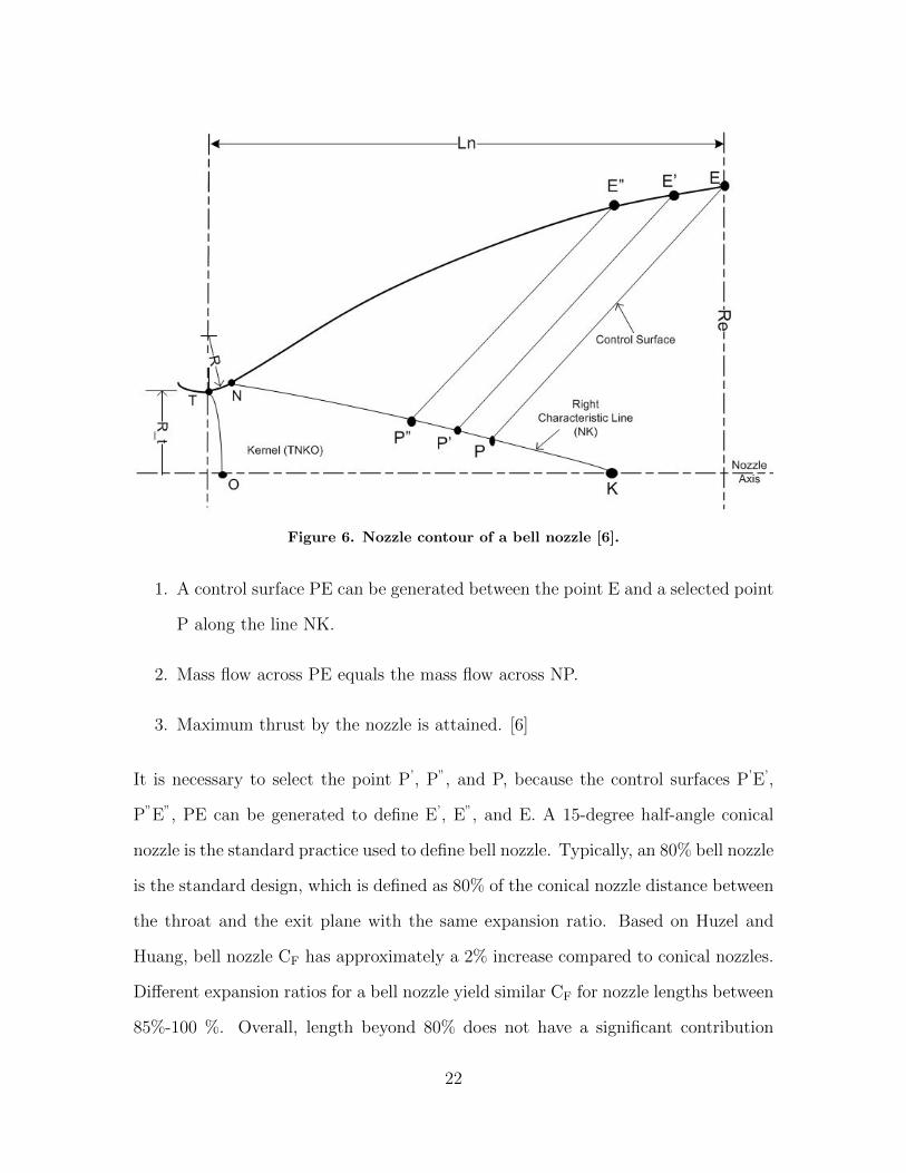
Figure 6. Nozzle contour of a bell nozzle [6].

1. A control surface PE can be generated between the point E and a selected point

P along the line NK.

2. Mass flow across PE equals the mass flow across NP.

3. Maximum thrust by the nozzle is attained. [6]

It is necessary to select the point P’, P”, and P, because the control surfaces P’E’,

P”E”, PE can be generated to define E’, E”, and E. A 15-degree half-angle conical

nozzle is the standard practice used to define bell nozzle. Typically, an 80% bell nozzle

is the standard design, which is defined as 80% of the conical nozzle distance between

the throat and the exit plane with the same expansion ratio. Based on Huzel and

Huang, bell nozzle CF has approximately a 2% increase compared to conical nozzles.

Different expansion ratios for a bell nozzle yield similar CF for nozzle lengths between

85%-100 %. Overall, length beyond 80% does not have a significant contribution

22

toward performance, but it adds additional weight [6] [20].

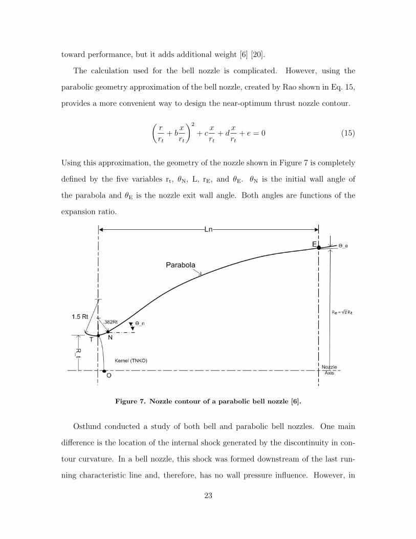
The calculation used for the bell nozzle is complicated. However, using the

parabolic geometry approximation of the bell nozzle, created by Rao shown in Eq. 15,

provides a more convenient way to design the near-optimum thrust nozzle contour.

(r

rt+ b

x

rt

)2

+ cx

rt+ d

x

rt+ e = 0 (15)

Using this approximation, the geometry of the nozzle shown in Figure 7 is completely

defined by the five variables rt, θN, L, rE, and θE. θN is the initial wall angle of

the parabola and θE is the nozzle exit wall angle. Both angles are functions of the

expansion ratio.

Figure 7. Nozzle contour of a parabolic bell nozzle [6].

Ostlund conducted a study of both bell and parabolic bell nozzles. One main

difference is the location of the internal shock generated by the discontinuity in con-

tour curvature. In a bell nozzle, this shock was formed downstream of the last run-

ning characteristic line and, therefore, has no wall pressure influence. However, in

23

a parabolic bell nozzle, this shock formed upstream of the characteristic line, and it

affects the flow properties at the wall. This caused a slightly-higher exit wall pressure.

For this reason, the parabolic nozzle has proven useful for sea-level nozzles, where the

flow separation margin improvement is important [6] [20].

2.3 Low Reynolds Number Nozzle Performance

In the low Reynolds number region, a large portion of the flow area is occupied by

the flow boundary layer. The relative increase of viscous losses can reduce thruster

performance. Rothe performed electron-beam studies of low Reynolds number flows

between 100 and 1500 in 1970. The studies were conducted using a conical nozzle with

a 20-degree wall angle. The results of his studies indicated that for Reynolds number

greater than 500, a small inviscid core existed in the flow. As the Reynolds number

increased close to 1,000, the core extended to the nozzle exit. With lower Reynolds

numbers, axial density and pressure gradients became less steep. Also, for Reynolds

number ranges from 500-1000, the centerline temperatures decrease monotonically

from the throat to the exit. In addition, his studies determined for Reynolds numbers

below 300, the flow is fully viscous with no indication of any inviscid core. Overall,

Rothe found significant negative radial pressure gradients exit throughout the nozzle

for Reynolds numbers ranging from 100-1500 [25].

Murch and Broadwell also conducted performance studies with heated nitrogen

and hydrogen on low thrust and low Reynolds number nozzles to determine the de-

pendence of thruster performance on nozzle geometry. These studies were conducted

using 10- , 20- , and 30- degree conical nozzles, bell nozzles, and horn nozzles. The re-

sults of the studies indicated nozzle efficiencies for different area ratios dropped from

94% to 90% as Reynolds numbers decreased from 2900 to 600. The nozzle efficiency

in this case defined as the ratio of the actual specific impulse to the specific impulse

24

of a frictionless nozzle with the same area ratio. The efficiencies also decreased with

an increase in area ratio. Studies also indicated for lower Reynolds numbers, an in-

crease in area ratio may not produce an increase in specific impulse. In performance

comparison between different half angles, the 20 degree nozzle produced the highest

efficiency, while the 35-degree nozzles were the poorest due to divergence losses [18].

Grisnik and Smith performed experimental studies on high-performance elec-

trothermal thrusters operating in a low Reynolds number region [4]. These studies

were conducted using a conical, bell, trumpet, and modified trumpet nozzle. Similar

to previous low Reynolds number studies, the nozzles indicated significant decreases

in specific impulse efficiency with decreasing Reynolds numbers. These studies of the

four nozzles also concluded that changes in the divergent contour do not affect the vis-

cous and divergent losses to any appreciable extent. All four nozzles were filled with

a large boundary layer. [4] Shorter expansion lengths were advantageous at very low

Reynolds numbers for improving performance and reducing thruster size and weight.

The flow through a shorter nozzle exhibits a thinner boundary layer near the nozzle

exit [9].

Regarding nozzle geometry, Hopkins and Hill developed a method to numerically

predict the flow field in the transonic region of nozzles [5]. Their studies indicated

the most significant geometric factor influencing the transonic flow pattern is the wall

radius of curvature in the throat region. The curvature of the throat significantly al-

tered the shape of the sonic line. When the radius of curvature was less than the

throat radius, an inflection point occurred in the sonic line. The effect of convergent

angle had on the throat flow was insignificant unless the wall radius of curvature was

less than the throat radius [5]. Moreover, other low Reynolds number flow studies

included considering the discharge coefficient. Kuluva and Hosack examined the dis-

charge coefficient of micro-thruster propulsion nozzles at low Reynolds numbers. The

25

results showed that the effect of velocity slip on the discharge coefficient is significant

at throat Reynolds numbers less than about 103. The effect of curvature becomes

important at Reynolds numbers on the order of 2 x 102 [11].

In 1987, Whalen conducted an experimental performance study on low Reynolds

number flows of 15- , 20- , and 25- degree conical nozzles, bell nozzles, and trumpet

nozzles with unheated nitrogen and hydrogen. The main goal of this study was to

evaluate and compare the performance of different nozzle contours. Specific impulse

efficiency and discharge coefficients for each nozzle as a function of Reynolds numbers

were evaluated for different area ratios and nozzle contours [32].

The results indicated at Reynolds numbers below approximately 2000, bell contour

nozzles tended to have a lower efficiency than the other contours. The trumpet and

25- degree conical nozzles performed slightly better than the other nozzles. For high-

area ratios, the trumpet and 25- degree conical nozzles performed significantly better

than the bell nozzles. Therefore, the bell nozzles, as designed, were not recommended

for low Reynolds number nozzles. For small nozzles, performance differences between

different contours were small. If this small difference was the not the major driver

for the thrusters application, then it is better to design nozzles based on the ease of

fabrication [32].

Spisz et al. conducted studies regarding the performance losses associated with low

Reynolds numbers, low flow rates, and low thrust nozzles [26]. The results indicated

at low Reynolds numbers, the thrust coefficients were lower than the thrust coefficient

calculated for isentropic flow through a choked orifice. In addition, even though large-

area ratio usually helped increase performance, in the case of low Reynolds numbers,

large area ratios were not required for achieving maximum thrust [26]. Figure (32) is

a recreated figure of Spisz’s studies data and the figure illustrates effects area ratio

had on thrust coefficient for different Reynolds numbers. For Reynolds number equal

26

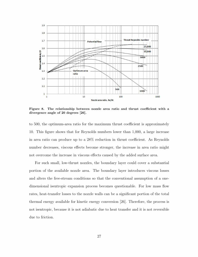
Figure 8. The relationship between nozzle area ratio and thrust coefficient with adivergence angle of 20 degrees [26].

to 500, the optimum-area ratio for the maximum thrust coefficient is approximately

10. This figure shows that for Reynolds numbers lower than 1,000, a large increase

in area ratio can produce up to a 28% reduction in thrust coefficient. As Reynolds

number decreases, viscous effects become stronger, the increase in area ratio might

not overcome the increase in viscous effects caused by the added surface area.

For such small, low-thrust nozzles, the boundary layer could cover a substantial

portion of the available nozzle area. The boundary layer introduces viscous losses

and alters the free-stream conditions so that the conventional assumption of a one-

dimensional isentropic expansion process becomes questionable. For low mass flow

rates, heat-transfer losses to the nozzle walls can be a significant portion of the total

thermal energy available for kinetic energy conversion [26]. Therefore, the process is

not isentropic, because it is not adiabatic due to heat transfer and it is not reversible

due to friction.

27

2.4 Water electrolysis systems and process

The water electrolysis system uses deionized water as fuel in a low-pressure tank.

A membrane feeds the water to an electrolyzer. Through the electrolysis process,

the water absorbs the electrical energy and decomposes into gaseous hydrogen and

oxygen by ion exchange. Hydrogen and oxygen gases will go into separate tanks

before entering the injector for combustion [27].

Currently, no water electrolysis system in a CubeSat has flown in space yet, but

the concept and design of a water electrolyzer is not a new development. In 1973, the

initial water electrolysis system test and studies were first introduced by Stechman,

et al. They conducted the study by using two different engines: one produced 22 N of

thrust and the second one, which was a scaled-down version of the first one, produced

0.445 N of thrust. Electrical current passed through a plastic membrane that was

saturated with water to create ion exchange. The ion exchange membrane performed

as a Solid Polymer Electrolyte (SPE) without requiring another electrolytic agent

such as acid or alkaline fluids. A SPE was in charge of the conduction of protons,

electrical insulation, and product gases separation. The electrolysis system consisted

of a cathode, an anode, a water feed barrier, and a SPE. A drawing of this system is

shown in Figure 9, and the electrolysis process is shown in Figure 10 [27].

The deionized water first entered through a water feed barrier (WFB). This WFB

acted like the SPE with the exception that it was without electric current. The

reactant water first passed through the WFB to enter the cathode side of the wall.

The water diffused across the SPE to the anode side for the electrolysis process. The

cathode and anode created a gradient across the SPE. This gradient increased the

electrical resistance in SPE and lowered the water activity at the anode. At the

anode, the first electrolysis process occurred with a chemical reaction shown in Eq.

28

Figure 9. Schematic Diagram of Electrolysis Cell [27].

(16), and released gaseous oxygen.

2H2O → 4H+ + 4e+ +O2(g) (16)

A manifold adjoining the anode side was connected to an oxygen plenum tank, where

the released oxygen gas would transfer. The SPE was created such that only the

passage of protons is allowed to go through, but the passage of hydrogen or oxygen

gas was prohibited. The SPE allowed the separation of gases to occur. After the

gaseous oxygen was released, 4H+, hydrogen traveled back to the cathode side, where

the second electrolysis process occured with the chemical reaction described by Eq.

(17), which releases hydrogen gas.

4H+ + 4e→ H2(g) (17)

A manifold adjoining the cathode side was connected to a hydrogen plenum tank,

29

Figure 10. The electrolysis process [27].

30

where the released hydrogen gas would transfer. The hydrogen and oxygen were

stored in different tanks before going through the injector for combustion [27].

Different organizations have also developed their own water electrolysis thrusters.

Cornell University has developed a 2U prototype thruster with three main compo-

nents: water tank with electrolysis, combustion chamber, and nozzle [35]. This 2U

system was tested in a 3U CubeSat to determine the amount of ∆V it can produce.

This electrolysis system used a proton exchange membrane, which is different from

the Stechman et al. electrolyzer system. Distilled water can be used as propellant

to replace deionized water because the PEM electrolyzer does not require dissolved

electrolytes in the water. In this design, the products of gaseous hydrogen and oxy-

gen from the electrolysis process would both remain in the storage tank instead of a

separate hydrogen and oxygen tank. Electrolysis increases the pressure of the water

tank as the amount of gas increases. Once the oxygen and hydrogen mixture reaches

the required pressure, 10 bar or higher, a solenoid value would allow the mixture into

the combustion chamber. A small spark plug is used to combust the gas mixture in

the combustion chamber. According to prototype testing reported by Zeledon and

Peck, the thruster was able to provide an average ∆V of 1.9 m/s per burst for the

3U CubeSat and an estimated 350 sec of specific impulse [35][36].

NASA LeRC Group, Hamilton Standard, and Lawrence Livermore National Lab-

oratory also developed and tested an electrolysis propulsion system. This system used

the sulfonic acid PEM as the sole electrolyte. This electrolysis cell consisted of a water

feed chamber, a water permeable membrane, a hydrogen chamber, a SPE membrane,

an oxygen chamber, an electrochemical hydrogen pump, and electrical insulators on

both end plates. This system was very similar to Stechman’s model described earlier.

For this study, two flight-type thrusters with different mass and a 23.3 expansion

ratio were built. A 22N thruster demonstrated over 69,000 firings with a total burn

31

time of four hours, and it produced a specific impulse of 355 sec at 50 psia cham-

ber pressure. The second one for the same program, a 0.5 N thruster, demonstrated

over 150,000 firings with a total burn time of 10 hours, and it produced a specific

impulse of 331 sec at 80 psia chamber pressure. Their studies showed an increase in

storage pressure also increased the required power and generation rates. However,

the electrolysis conversion efficiency decreased gradually with increasing electrolysis

pressure, due to the energy required for gas compression and the internal hardware

configuration. Therefore, a tradeoff was required for the propulsion system between

better efficiency and higher electrolysis pressure. The average electrolyzer efficiency

is defined as the minimum power theoretically required for water electrolysis divided

by the actual power used. This remaining power is rejected as heat. According to

McElroy, typical efficiency values for electrolysis was between 85 and 90% [16].

2.5 Hydrogen-Oxygen Combustion

The water electrolysis thruster uses the gaseous hydrogen and oxygen for combus-

tion to produce water vapor. This stoichiometric reaction is shown below.

2H2(g) +O2(g)→ 2H2O(g) (18)

This reaction is a global reaction, and it does not happen directly. In order to make

this global conversion of hydrogen and oxygen to water occur, elementary reactions

need to happen first. The four reactions listed below are the main elementary reac-

tions.

H2 +O2 → HO2 +H (19)

H +O2 → OH +O (20)

OH +H2 → H2O +H (21)

32

H +O2 +M → HO2 +M (22)

When hydrogen and oxygen molecules first collide and react, they do not produce

water. In fact, it was shown in reaction (19) that hydrogen and oxygen molecules

collide and produce HO2 and H. HO2 is the intermediate species. During this reaction

process, only one bond is broken, and one bond is formed. H2 and O2 forming two

OHs is unlikely because it requires breaking and creating two bonds [30].

A collection of elementary reactions necessary to describe an overall reaction is

called a reaction mechanism. In the case of hydrogen-oxygen combustion, this reaction

mechanism has as much as 40 reactions and involves eight species: H2, O2, H2O, OH,

O, H, HO2, and H2 O2. The H2-O2 system not only plays an important role in rocket

propulsion, but it is also an important subsystem in the oxidation of hydrocarbons

and moist carbon monoxide [30]. H2-O2 mechanism consists of initiation, branching,

recombination, and diffusion. The initiation reactions are:

H2 +M → H +H +M (23)

H2 +O2 → HO2 +H (24)

Initiations are related to hydrogen dissociation, because the dissociation energy of

hydrogen is lower than that of oxygen. Only a few radicals are required to initiate the

explosion in the 675 K temperature region. Reaction (23) is for higher temperatures,

and it requires about 435 kJ/mol. Reaction (24) is for other temperatures, and it has

a lower energy requirement of only 210 kJ/mol. The main feature of the initiation

step is to provide a radical for the chain system [3].

Next is the chain branching state. The chain reactions are shown below, and they

33

involve O, H, and OH radicals.

H +O2 → O +OH (25)

O +H2 → H +OH (26)

H2 +OH → H2O +H (27)

O +H2O → OH +OH (28)

For reaction (26), the H radical is generated, and there is no chemical mechanism

barrier to prevent the system from being explosive. The reverse reactions for (25),

(26), and (28) are negligible because their concentration levels in many systems are

very low. Apart from chain branching, reactions (25)- (28) also provide the essential

propagating steps and the radical pool for fast reactions. [3]

The explosion limit for hydrogen-oxygen mixture is shaped like a reverse S-curve.

Figure 11 shows the explosion limit curve for a stoichiometric hydrogen-oxygen mix-

ture. This is a branched-chain explosion. The explosion limits must be specified

in terms of the chemical-kinetic and diffusion parameters that determine the rates

of chain branching and chain breaking notably temperature, pressure, mixture com-

position, and environmental conditions. In the explosive region, the rate of chain

branching is greater than the rate of chain breaking. In the no explosion region, the

relationship is reversed. At the limit line, the two rates are equal [13].

H and OH wall destructions are important chain termination steps.

H → wall destruction

OH → wall destruction

These two steps explain the lower limit of hydrogen-oxygen mixture explosion. Wall

34

Figure 11. Explosion limits of a stoichiometric hydrogen-oxygen mixture [13]

collisions are more predominant at a lower pressure compared to molecular collisions.

The second explosive limit is caused by gas phase production and destruction of

radicals. For this to occur, the most effective chain-branching reaction, which is

reaction (25), must be overridden by another reaction step. When a system with a

fixed temperature is moving from a lower pressure to a higher pressure, the system

transitions from an explosive state to a steady reaction condition, which is the other

side of the second limit. The reaction step that overrides the chain-branching reaction

must be more pressure sensitive [3].

The existence of the second explosion limit is readily explained if the three-body

35

reaction is added to the scheme. This reaction is:

H +O2 +M → HO2 +M (29)

where M denotes any third molecule that stabilizes the combination of H and O2. The

free radical HO2 is considered to be relatively unreactive, so that it is able to diffuse

to the wall and become a means for effectively destroying H radicals. Reaction (29)

does not require activation energy. Therefore, a range of temperatures and pressures

exists at which the two reactions proceed at equal rates. According to the Arrhenius

function of the chain-branching reaction, the limit pressure increases with increasing

temperature, because the chain-branching rate increases with increasing temperature.

[13]

The upper third explosion limit is caused by a reaction that overtakes the stability

of the HO2.

HO2 +H2 → H2O2 +H (30)

Higher temperatures are required for reaction (30) to become effective, because the

reactivity of HO2 is much lower than OH, H, or O. Due to some resonance energy

exchange with the HO2 formed, water vapor tends to inhibit explosion due to the

effect of reaction (29), in that H2O has a high third-body efficiency [3]. Reaction (29)

is a recombination step requiring a third body, M, so its rate decreases with increas-

ing temperature. Conversely, reaction 16 increases with temperature. Thus, it can

be concluded that reaction (29) is more effective at higher pressures and lower tem-

peratures, while reaction (25) dominates at higher temperatures and lower pressures.

Therefore, at temperatures above 875 K, where the third explosion limit starts, reac-

tion 16 always prevails, and the mixture is explosive for the complete pressure range

covered.

36

In this third-limit explosion regime, the chain-terminating steps involving O, H,

and OH radicals are the three-body recombination reactions. The main gas-phase

termination steps are the following [3]:

H +H +M → H2 +M (31)

O +O +M → O2 +M (32)

H +O +M → OH +M (33)

H +OH +M → H2O +M (34)

In order to complete the mechanism, reaction (29) needs to occur again to produce

more HO2 [30]. After reaction (29), HO2 may be consumed in the H2-O2 system by

various radicals. The reactions are as follows:

HO2 +H → H2 +O2 (35)

HO2 +H → OH +OH (36)

HO2 +H → H2O +O (37)

HO2 +H → O2 +OH (38)

HO2 +OH → H2O +O2 (39)

Then, the HO2 radicals will recombine with each other to yield H2O2.

HO2 +HO2 → H2O2 +O2 (40)

Afterward, H2O2 will consumed by reactions with radicals and go through thermal

37

decomposition [30][3].

H2O2 +OH → H2O +HO2 (41)

H2O2 +H → H2O +OH (42)

H2O2 +H → HO2 +H2 (43)

H2O2 +M → 2OH +M (44)

Finally, although reaction (29) was acting as a chain-terminating step under some

conditions, especially at high temperature, under other conditions it is part of a chain

propagating path to obtain the final H2O product.

38

III. Test Methodology and Procedures

3.1 Introduction

This chapter reviews the equipment and connections set-up necessary to perform

vacuum testing of the HYDROSTM thruster. This research was performed in the en-

vironmental testing facility located at the Air Force Institute of Technology (AFIT).

A torsional balance thrust stand was used to capture impulse bit data. In order

to record the proper measurements, calibration of the thrust stand prior to testing

was required. The nozzle designs for this research were modeled using a nominal

two-dimensional conical geometry. The theoretical data calculation method was pre-

sented in Chapter 2. The theoretical data was calculated in this chapter. Lastly,

the comparison between the theoretical data and experimental data are presented in

Chapter 4.

3.2 Equipment and Connections

3.2.1 Vacuum Chamber.

The main equipment for this experiment included a vacuum chamber, thruster,

and thrust stand. The vacuum chamber for this research, shown in Figure 12, is a

horizontally-mounted chamber by PHPK Technologies. This chamber is capable of

pumping down to 10−4 Torr. This chamber opens by the door located in the front side

of the chamber. There is a sliding table located inside the chamber, which allows easy

assess to equipment. This vacuum chamber has a 60” diameter and is approximately

60” long. It is constructed of 3/8” thick 304 series stainless steel mounted to a painted

steel base. Vacuum feedthroughs are located around the chamber, as well as the back

side of the chamber. A five-inch feedthrough with two DB15 sub-connections was

used for this research. Connections for both sides are shown in Figure 13. A window

39

Figure 12. Space simulator vacuum system.

Figure 13. Vacuum to lab connections.

is also located on the back side of the chamber, which allows for visibility inside the

chamber for camera set-up. This is shown in Figure 14.

40

Figure 14. The window and passthrough location.

3.2.2 Torsional Balance Thrust Stand.

Thrust stand selection is critical for this research in order to obtain repeatable

and accurate results. This thruster does not produce a steady state force; rather,

it produces an impulse force. The selected thrust stand must have a high-frequency

sensor capable of capturing an approximately 0.3-second impulse. In addition, the

thrust stand is required to measure a thrust event between 0.1-0.5 N. A torsional

balance thrust stand by Tethers Unlimited Inc. was selected for this research. Unlike

the inverted pendulum thrust stand, a torsional balance thrust stand’s rotational axis

41

is parallel to the gravity vector, making its response less dependent on thruster mass.

This makes it ideal for measuring the HYDROSTM, because the thruster mass is not

constant throughout testing. Research studies had shown that torsional thrust stands

were inherently more stable than inverted-pendulum thrust stands and offer a balance

of high-thrust measurement sensitivity and low-environmental noise sensitivity [22].

Research from Koizumi, Komurasaki, and Arakawa measured that the overall thrust

stand impulse accuracies are typically 2.1µN-s for an impulse range of 20-80 µN-s and

0.7µN-s for an impulse range of 1-10N-s [10].

This torsional balance thrust stand consists of a swinging arm used to mount

the thruster. The swinging arm is divided by a centerline, where the counterweights

are located on both ends of the arm. The counterweights are placed on the arm for

balance and to ensure the arm is parallel to the sensor. The center axis is mounted

to a frame via two torsional springs. An image of the complete set-up is shown in

Figure 15.

Figure 15. Rotational balance thrust stand with thruster.

The thruster is mounted horizontally to the left of the center line. While the

42

calibration hammer and linear displacement sensor (LDS) are not directly mounted

on the swinging arm, they are located on the right side of the centerline. The hammer

has an integrated piezoelectric force transducer and is used for calibration purposes

prior to each set of tests. Research from Pancotti and Hilario showed piezoelectric

hammers have linearity within 0.99% for a range of of 10 mN-s to 750 mN-s [21]. A

motor is used to control the hammer. A detailed image of the hammer and its motor

are shown in Figure 16. The hammer provided an impulse force to the thrust stand

Figure 16. Calibration hammer and motor.

and the LDS is used to measure the response to a known impulse input from the

hammer. When the thruster is fired on the thrust stand, the LDS will measure the

displacement response in voltage through Labview. The calibration data can measure

the impulse bit of the thruster. A micro-adjuster is located below the LDS. The set-

up of the LDS and its adjuster are shown in Figure 17. The total set-up of the whole

system inside the vacuum chamber is shown in Figure 18.

43

Figure 17. LDS and micro-adjuster.

Figure 18. Thruster stand and thruster inside the vacuum chamber.

3.2.3 Thruster.

The thruster used for this experiment is the HYDROSTM thruster, shown in Fig-

ure 19. This 1U configuration thruster has an empty mass of 0.875 kg and is capable

of storing approximately 0.075 kg of water. This thruster is comprised of six main

components: a water tank, a H2 gas tank, an O2 gas tank, an injector, a combustion

chamber, and a nozzle. Water breaks down through the electrolysis process to create

gaseous hydrogen and oxygen. The hydrogen gas and oxygen gas store separately

44

Figure 19. The HYDROSTM thruster used for this research.

before entering the injector for combustion. The hydrogen gas tank has a volume of

12.9 cm3, and the oxygen gas tank has a volume of 6.6 cm3.

In order to fire the thruster, a computer running Labview sends commands and

receives data from the thruster. The computer is connected to a data acquisition

device (DAQ), used to convert the wire signals from digital to analog and also from

analog to digital. The DAQ is connected to an Arduino board. The Arduino board

communicates and runs the thruster. The Labview screen is shown in Figure 20.

There are four controls to the thruster: pressurize, vent, emergency hydrate, and

fire. The thruster is only fired after it reaches a commanded pressure. During the

normal pressurizing process, the electrolyzer voltage runs at approximately 2.3 V

and the electrolyzer current draws between 0.3 and 1 A. Under these conditions, the

pressurization time is about two to three minutes per fire. The electrolyzer current

drops after each firing. After approximately eight firings, the electrolyzer current

45

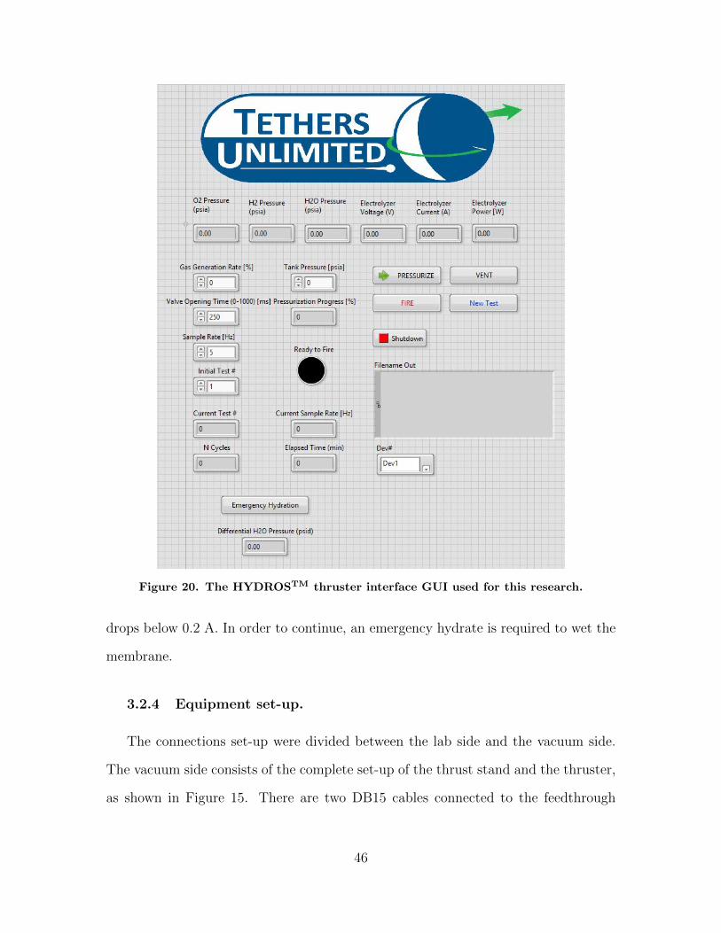
Figure 20. The HYDROSTM thruster interface GUI used for this research.

drops below 0.2 A. In order to continue, an emergency hydrate is required to wet the

membrane.

3.2.4 Equipment set-up.

The connections set-up were divided between the lab side and the vacuum side.

The vacuum side consists of the complete set-up of the thrust stand and the thruster,

as shown in Figure 15. There are two DB15 cables connected to the feedthrough

46

on the vacuum side labeled Chamber-A and Chamber-B. The Chamber-A connector

connected to the thruster’s Arduino board and the LDS. The chamber-B connector

is connected to the hammer and motor.

On the lab side, there is a PCB signal conditioner, two power supplies, a calibration

Arduino board, a Data Acquisition (DAQ) system, and a laptop. The set-up is shown

in Figure 21. All of this equipment was connected through two 15 pin bundle cables

Figure 21. The lab side set-up.

similar to the vacuum side. They were labeled Lab-A and Lab-B, and connected to

Chamber-A and Chamber-B respectively. Lab-A was connected to the DAQ system,

and it sent and received signals to the thruster’s Arduino board. The DAQ system

was connected to the labtop to run Labview. A power supply up to 10-volt and

1.5-amp was required for the thruster.

Lab-B was used to communicate with the hammer and motor on the vacuum side.

The signals from the hammer went through the PCB signal conditioner. The output

of these signals was connected to the DAQ system. Another Arduino board was used

to control the hammer’s motor, and required a 24V power supply. A diagram of the

47

complete set-up is shown in Figure 22.

Figure 22. The complete experiment set-up.

After all the cables were connected properly, testing was performed in vacuum.

Prior to each vacuum pump down, the measurement of the thruster’s mass was im-

portant. It was critical to keep track of how much fuel was used during a firing set for

later calculations. In addition, before the vacuum was pumped down, the adjustment

of the counterweights’ position to ensure the swinging arm was parallel to the LDS

was also critical. This is shown in Figure 23. Furthermore, it was important to ensure

the LDS was in the correct position relative to the swinging arm. The displacement

voltage on the Labview screen should read 5V (+/- 0.5V). If the voltage was not

5V, then the LDS required adjustment through the micro-adjuster attached below

the LDS. This could only be adjusted in atmosphere manually. Finally, the vacuum

chamber was ready to pump down for experiments.

A HPV2 high-speed camera was used to capture the thruster’s exhaust plume.

This camera was used to capture high-speed images up to a million frames per second

at intensity gains up to 50x. The camera can records 102 frames at a time. The set-up

48

Figure 23. Swinging arm with LDS.

of the camera is shown in Figure 24. The camera is triggered by the fire signal from

the Labview VI. For this experiment, all images were captured at 250 or 500 frames

per second. The time delay between sending the pressurization command and the

moment ignition occured apparently changed each time, thus, it was very difficult to

capture the firing faster than 500 frames per second.

49

Figure 24. The camera set-up.

3.3 Calibration of Torsional Balance Thrust Stand

After the vacuum chamber was pumped down, before each testing set, thruster

calibration was required to determine how the thrust stand responded to a known

force. The purpose of this calibration was to properly measure the impulse bit of

the thruster. The calibration determined the response to an impulse force. Thus,

this response can be used to calculate the impulse force of the thruster. A set-up

diagram, shown in Figure 25, displays a more simplified diagram of the thrust stand

for reference.

50

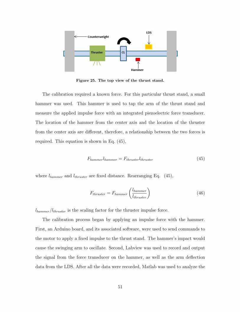
Figure 25. The top view of the thrust stand.

The calibration required a known force. For this particular thrust stand, a small

hammer was used. This hammer is used to tap the arm of the thrust stand and

measure the applied impulse force with an integrated piezoelectric force transducer.

The location of the hammer from the center axis and the location of the thruster

from the center axis are different, therefore, a relationship between the two forces is

required. This equation is shown in Eq. (45),

Fhammerlhammer = Fthrusterlthruster (45)

where lhammer and lthruster are fixed distance. Rearranging Eq. (45),

Fthruster = Fhammer

(lhammerlthruster

)(46)

lhammer/lthruster is the scaling factor for the thruster impulse force.

The calibration process began by applying an impulse force with the hammer.

First, an Arduino board, and its associated software, were used to send commands to

the motor to apply a fixed impulse to the thrust stand. The hammer’s impact would

cause the swinging arm to oscillate. Second, Labview was used to record and output

the signal from the force transducer on the hammer, as well as the arm deflection

data from the LDS. After all the data were recorded, Matlab was used to analyze the

51

relationship between arm deflections and impulse bits.

Figure 26. Hammer impulse response.

Figure 26 shows an impulse response from the LDS. This response is a sinusoid

impulse response with an exponential decay from dampening. The estimated equation

of this response is shown in Eq. (47),

y(t) = Asin(ωnt)e−ξωnt (47)

where A is the amplitude in Volts, t is the time in seconds, ξ is the damping ratio,

and ωn is the natural frequency of the system. A, ξ, and ωn are the three unknown

in the equation. The amplitude at approximately one second in Figure 26 is lower

than the overall response amplitude due to the effects of damping.

52

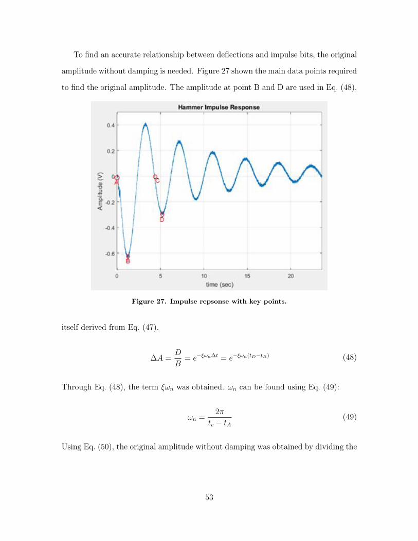
To find an accurate relationship between deflections and impulse bits, the original

amplitude without damping is needed. Figure 27 shown the main data points required

to find the original amplitude. The amplitude at point B and D are used in Eq. (48),

Figure 27. Impulse repsonse with key points.

itself derived from Eq. (47).

∆A =D

B= e−ξωn∆t = e−ξωn(tD−tB) (48)

Through Eq. (48), the term ξωn was obtained. ωn can be found using Eq. (49):

ωn =2π

tc − tA(49)

Using Eq. (50), the original amplitude without damping was obtained by dividing the

53

measured amplitude by e−ξωn∆t.

Aoriginal =Ameausurede−ξωn(tB−tA)

(50)

A new curve is plotted using the original amplitude with the estimated equation.

Eq. (51) is the equation for this new curve.

yoriginal(t) =Ameasurede−ξωn(tD−tB)

sin(ωnt)e−ξωnt (51)

A comparison between the measured response and the new response is shown in

Figure 28.

Figure 28. The measured response and the new response with the original amplitude.

Before finding a unit response, both amplitude and time need to off-set back to

zero. After finding the new response with the undamped amplitude, this response is

used to obtain a unit response. First, the impulse bit of the hammer input needed to

be found. An example of the hammer input is shown in Figure 29.

54

Figure 29. An impulse input from the hammer.

The trapezoidal numerical integration method was used to determine the impulse

bit of the hammer impulse. The equation for calculating the unit-response is shown

in Eq. (52).

Unit− response =yoriginal(t)

ibit(52)

The unit response represents the impulse response for one N-s of impulse. This unit

response is used to compare the impulse response of the thruster in order to determine

the impulse bit of the thruster. Figure 30 shows an example of the hammer unit

response.

55

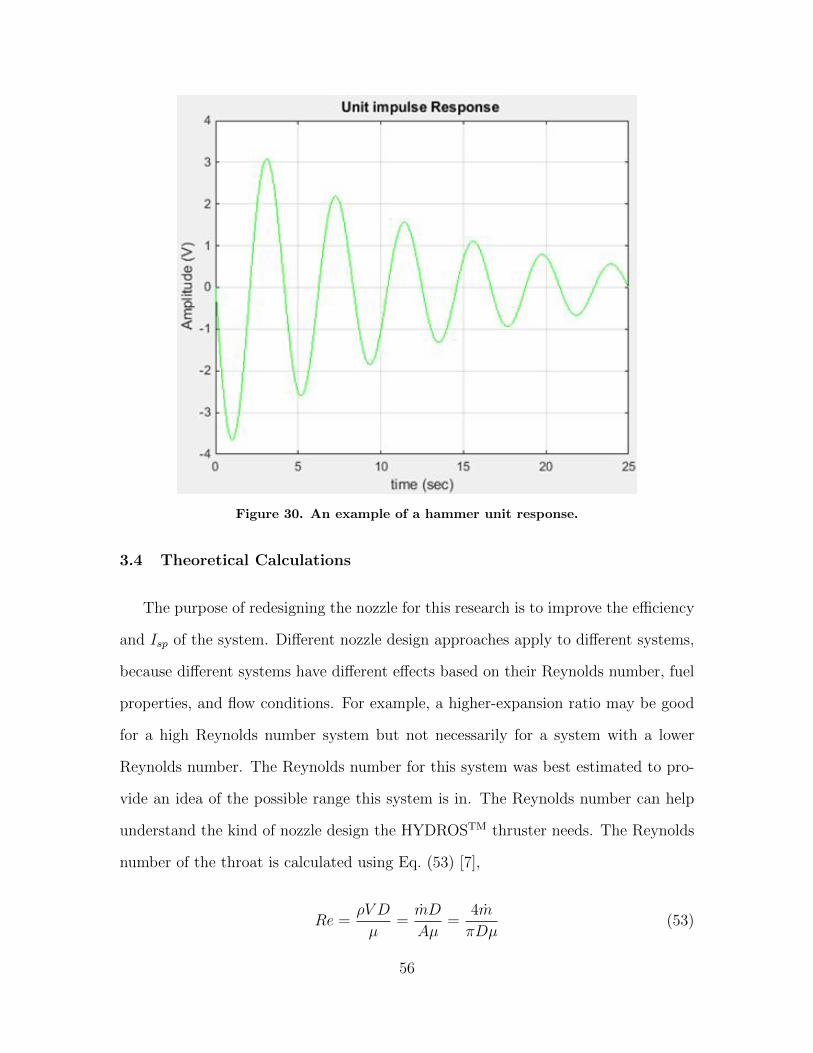
Figure 30. An example of a hammer unit response.

3.4 Theoretical Calculations

The purpose of redesigning the nozzle for this research is to improve the efficiency

and Isp of the system. Different nozzle design approaches apply to different systems,

because different systems have different effects based on their Reynolds number, fuel

properties, and flow conditions. For example, a higher-expansion ratio may be good

for a high Reynolds number system but not necessarily for a system with a lower

Reynolds number. The Reynolds number for this system was best estimated to pro-

vide an idea of the possible range this system is in. The Reynolds number can help

understand the kind of nozzle design the HYDROSTM thruster needs. The Reynolds

number of the throat is calculated using Eq. (53) [7],

Re =ρV D

µ=mD

Aµ=

4m

πDµ(53)

56

where m is the mass flow rate in kilogram-per-second calculated, D is the diameter

of the throat in meters, and µ is the dynamic viscosity of the gas in Pascal-second.

The Reynolds number calculation, dynamic viscosity, and all other combustion

conditions are approximated using Chemical Equilibrium with Applications (CEA).

The CEA calculations were based on a 20% drop of a 49-psi plenum pressure, which is

about 40-psi chamber pressure. The oxidizer-to-fuel ratio for hydrogen-oxygen com-

bustion is 8, due to a stoichiometric combustion assumption. The dynamic viscosity

from CEA is 1 x 10−4 Pa-sec. Using Eq. (53), the Re number becomes 2238. The

CEA data represents the ideal case for hydrogen-oxygen combustion. The ideal mass

flow rate was also calculated to compare to the mass flow rate based on the vacuum

data. Using Eq. (54),

m = ρAV (54)

with density of the throat, ρ = 9.57 x 10−2, the throat velocity, V = 1362.6 kg/s, and

the ideal mass flow rate, m = 1.6 x 10−4 kg/s.

Another criterion to investigate is the optimal expansion ratio. This is the theo-

retical maximum. An increase in expansion ratio can increase the thrust of a system

up to a limit. This maximum point is the optimal expansion ratio, where the exit

pressure is approximately equal to the ambient atmospheric pressure. The optimal

expansion ratio can help determine the maximum thrust, Isp, and the optimal thrust

coefficient of which this thruster is capable. However, these calculations are not as

accurate for this small-scale thruster, because these calculations do not include con-

ditions, such as incomplete combustion, and most importantly, viscous effects. The

optimal expansion ratio is calculated through the exit Mach number. Exit velocity is

57

required to obtain mach number. Eq. (55) is the equation for exit velocity.

V2 =

√√√√( 2k

k − 1

)RT1

[1−

(P2

P1

) k−1k

](55)

where the specific heat ratio, k, is 1.11 from CEA, P2 is assumed to be zero, the specific

gas constant, R, for water vapor is 461.4 Jkg−1k−1, and the chamber pressure, T1, is

3208 K from CEA. Using Eq. (55), the exit velocity is 5465.6 m/s. Using Eq. (56)),

M2 =V2√kRT2

(56)

the exit Mach number is infinite because T2 is close to zero. Finally, the optimal

expansion ratio is calculated using Eq. (57):

A2

At=

(k + 1

2

)− k+12(k−1)

[

(1 + k−1

2M2) k+1

2(k−1)

M] (57)

Since the temperature must drop to zero to provide an exit pressure of zero, the Mach

number must be infinite and, therefore, the area ratio must be infinite.

P2 equal to zero is the absolute best case. In order to obtain a more realistic

expansion ratio, a slightly different approach was used.

T2

T1

=

(P2

P1

) k−1k

(58)

Substitute Eq. (58) into Eq. (59) [28],

V2 =

√(2k

k − 1

)RT1

[1− T2

T1

](59)

where T2 is assumed to be the condensation point temperature of water vapor at 1

58

atm, 373 K. In addition, the specific heat ratio from CEA was on the low end. For

the second approach, specific heat ratio for water vapor of 1.3 is used instead. P2 is

also not equal to zero, because this would require all potential energy be converted

into kinetic energy. With this new approach, exit velocity becomes 3,367 m/s, the

Mach number becomes 7.12, and the optimal expansion ratio becomes 314. The 15-

degree conical nozzle length required to obtain an area ratio of 314 is 1.6 inches using

Eq. (60).

L =rt(√ε− 1) +Rn(sec(θ)− 1)

tan(θ)(60)

Maximum CF , T, and Isp are now calculated using the expansion ratio. Eq. (61) is

used to calculate CF .

CF =

√√√√ 2k2

k − 1

(2

k + 1

) k+1k−1

[1−

(P2

P1

) k−1k

]+P2 − P3

P1

A2

At(61)

Before solving for CF , Eq. (62) and Eq. (63) are used to find P2 in order to solve for

CF .

PtP1

=

[2

k + 1

] kk−1

(62)

P2

Pt=

(1 +

k − 1

2M2

)− kk−1

(63)

P2 is 0.0019 and CF is 1.88. After calculating CF , C∗ is required to obtain Isp. Using

Eq. (64),

C∗ =

√kRT1

k

√2

k+1

k+1k−1

(64)

C∗ is 1,823.3 m/s. Using Eq. (65),

Isp =C∗CFg0

(65)

59

the optimal Isp is 349 sec. Equation (66) is used to calculate the optimal thrust.

T = CFP1At (66)

The optimal thrust for this system is 0.6355 N. A summary of the result is shown in

Table 1. However, these optimal values in Table 1 do not represent the entire picture,

Table 1. Optimal Nozzle Conditions

k P2(Pa) CF Isp(sec) T(N) L(m) A2

AtM2

1.3 13.1 1.88 349 0.6355 0.04 314 7.12

because the calculations ignore viscous boundary layer effects in low Reynolds number

flow.

Futhermore, Spisz et al. have conducted thrust coefficient studies on low-thrust

nozzles for steady flow operations [26], The results from the studies indicated large

area ratios were not required for achieving maximum thrust for nozzles with low throat

Reynolds number (<10,000). Therefore, the HYDROSTM thruster might not require

a large expansion ratio to achieve maximum efficiency and performance. Figure 31,

a figure regenerated from Spisz et al. data, indicated for Reynolds number of 2500,

there was a loss of thrust coefficient due to viscous forces from 0.035 to 0.35, as

expansion ratio increased from 2 to 400. Losses also increase as the Reynolds number

decreased.

Spisz et al. also found the optimum thrust coefficient with area ratio for different

throat Reynolds numbers. These are the net thrust coefficients, which included vis-

cous losses. The optimal area ratio line is represented by the dash-line in Figure 32,

which was generated with similar data. The data indicated that the gains due to

the increased area ratio were less than the additional viscous losses imposed by the

increased surface area [26]. For the HYDROSTM thruster’s Reynolds number range,

based on this study, the optimum area ratio is approximately 22.

60

Figure 31. Loss in thrust coefficient due to viscous effects [26].

Figure 32. Thrust coefficient vs. expansion ratio for different Reynolds numbers [26].

61

3.5 Nozzle Designs

In order to improve the current HYDROSTM thruster nozzle design, it is important

to first observe the design of the factory nozzle. This nozzle is shown in Figure (33).

The original design is a bell nozzle with an expansion ratio, ε = 266. The expansion

Figure 33. CAD model of the factory nozzle

angle, α, is approximately 37 degrees. This nozzle is over-expanded at sea level and

has a high expansion ratio with a short length of 0.59 in. Based on the nozzle length

and expansion ratio, this design did not follow the nominal method of characteristics

(MOC) design for a bell nozzle, and has an excessive required turning angle just

downstream of the throat, resulting in separated flow.

The idea for the first nozzle design is to keep the original factory nozzle length.

Keeping the original length allows the nozzle not to extend beyond the 1U configu-

ration. This 15-degree conical nozzle was chosen because of its simplicity in design

and ease of fabrication. Using the two-dimensional conical nozzle geometry from

Huzel and Huang, a new expansion ratio was calculated using the existing length [6].

62

Eq. (60) needs rearrangement to obtain an equation in terms of ε shown in Eq. (67)

ε =

(Ltan(θ) +Rn(sec(θ)− 1)

rt+ 1

)2

(67)

where L is the nozzle length in inches, rt is the throat radius in inches, Rn is the

circular contour arc radius of the throat in inches, and θ is the expansion angle,

which is 15-degrees. To find Rn, Eq. (68) is used [6].

Rn = 0.382rt (68)

The throat radius is 0.0246 in. and Rn is 0.0094 in. The expansion ratio becomes

55 per Eq. (67). The geometry of the conical nozzle is shown in Figure 34. The

Figure 34. Nozzle contour of the conical nozzle [6].

nozzle was designed using commercial CAD software and manufactured at the AFIT

machine shop. Both the CAD and manufactured models are shown in Figure 35. The

material of the nozzle is aluminum 6061.

Using Eq. (57)-Eq. (66), the maximum thrust, coefficient of thrust, and Isp are

obtainable. These values will be used to compare with the experimental values to

observe the performance loss and efficiency of the nozzle. These values disregard

63

Figure 35. CAD and manufactured model for nozzle 1.

viscous losses in the nozzle area. Using an area ratio of 55 and k of 1.3, with Eq. (57),

the Mach number at the exit was calculated. Using this Mach number with Eq. (63)-

Eq. (62), P2 was determined. Then, the coefficient of thrust was calculated using

Eq. (61). After finding CF , Isp and T were calculated using Eq. (65) and Eq. (66).

The results of the calculations are shown in Table 2.

The second design is also a conical nozzle. This design kept the original factory

expansion ratio and evaluated the length required with a 15-degree expansion angle.

Using Eq. (60), the second nozzle length was determined. With a 266 expansion ratio,

the new length was 1.407 in. Using the contour shown in Figure 34 with the new nozzle

length, the design was created using CAD. Due to the length, nozzle 2 is extended

outside of the 1U configuration. Figure 36 shows the CAD and manufactured model

of nozzle 2. In order to calculate the ideal coefficient of thrust, Isp and thrust, the

same procedures from nozzle 1 calculations were repeated with nozzle 2 expansion

ratio. The results are shown in Table 2.

The purpose of the third nozzle is to evaluate a more optimal expansion ratio for

this system. Based on Spisz et al.’s research discussed previously [26], an expansion

ratio of 22 was chosen to match the optimum area ratio for the calculated Reynolds

64

Figure 36. CAD and manufactured model for nozzle 2.

number. This nozzle is expected to show a small improvement in Isp when compared

to nozzle 1 (ε = 55). The CAD model and manufactured model are displayed in

Figure (37). The outcome of this data can help determine if Spisz et al ’s. research

for low Reynolds number systems can also be applied to systems with short firing

duration.

Figure 37. CAD and manufactured model for nozzle 3.

The ideal coefficient of thrust,thrust, and Isp for this nozzle were calculated using

Eq. (57)- Eq. (66) and shown in Table 2. A summmary of the expansion ratio for the

65

Table 2. Optimal conditions for the three nozzle designs.

Nozzle k P2(Pa) CF T (N) Isp(sec)1 1.3 2 x 10−7 1.814 0.614 3372 1.3 2.4 x 10−8 1.873 0.634 3483 1.3 9.6 x 10−7 1.761 0.596 327

four nozzles is indicated in Table 14 and a comparison of all four nozzle contours is

shown in Figure 52.

Table 3. A summary of expansion ratios.

Original 1 2 3ε 266 55 266 22

(a) Original Nozzle. (b) Design 1. (c) Design 2. (d) Design 3.

Figure 38. Nozzles comparison of the 4 nozzles [15].

3.6 Error analysis

The performance criterion discussed in Chapter 4 include impulse bit, specific

impulse, and thrust coefficient. Impulse bit measurement variations were calculated

using standard error. The standard error was calculated using the Eq. (69),

SEx =S√n

(69)

66

where S is the standard deviation and n is the sample size. Using this standard error,

the impulse bit error was calculated using Eq. (70),

σIbitIbit

=

√(SEx

displacement

)2

(70)

where displacement is the displacement of the swinging arm in voltage. The equation

for Ibit is shown in Eq. (74),

Ibit =displacement

6.26(71)

where 6.26 is the calibration conversion number in V/N-s. For specific impulse, the

total error propagation is shown in Eq. (72),

σIspIsp

=

√(σibitibit

)2

+(σ∆m

∆m

)2(72)

where σ represents the error. Lastly, error propagation for CF was calculated using

Eq. (73). All error results are indicated in the data plots’ error bars in Chapter 4.

σCF

CF=

√(σIspIsp

)2

(73)

67

IV. Results and Analysis

The experimental set-up discussed in Chapter 3 was used to determine the per-

formance of the HYDROSTM thruster. Experimental results and data analysis are

presented in this chapter. The performance criteria for this research are impulse bit,

specific impulse, thrust coefficient, and exhaust plume attachment. Further perfor-

mance analyses are investigated through comparing the results between the experi-

mental data, the theoretical data from CEA, and the research data from Spisz et al.

Spisz et al. conducted research on the thrust coefficient for a low thrust, steady state,

and low Reynolds number thruster. Their research analyzed the influence viscous

effects have at different Reynolds numbers and expansion ratios. The experimental

data from this research were used to compare with Spisz et al.’s data to investigate

whether pulsed thrusters might display the same behavior identified in their research.

4.1 Thrust Stand Calibration Results

The thrust stand was originally calibrated by using a small calibration hammer

located on the thrust stand. This calibration hammer was used for the original

nozzle and nozzle 1. However, a different hammer was used to calibrate nozzle 2

and nozzle 3, due to a malfunction of the small hammer. The new hammer was not

attached to the electrical connections of the thrust stand; therefore, calibrations were

performed at atmospheric conditions instead of at vacuum. This research assumed

calibration behavior in atmosphere is similar to that in vacuum. This assumption was

possible because the main difference between calibrating at atmosphere and at vacuum

is aerodynamic drag. Since the thrust stand experiences very little displacement,

and has a very low natural frequency, due to the high moment of inertia of the

system, the velocity of the thrust stand is approximately zero. Thus, there is minimal

68

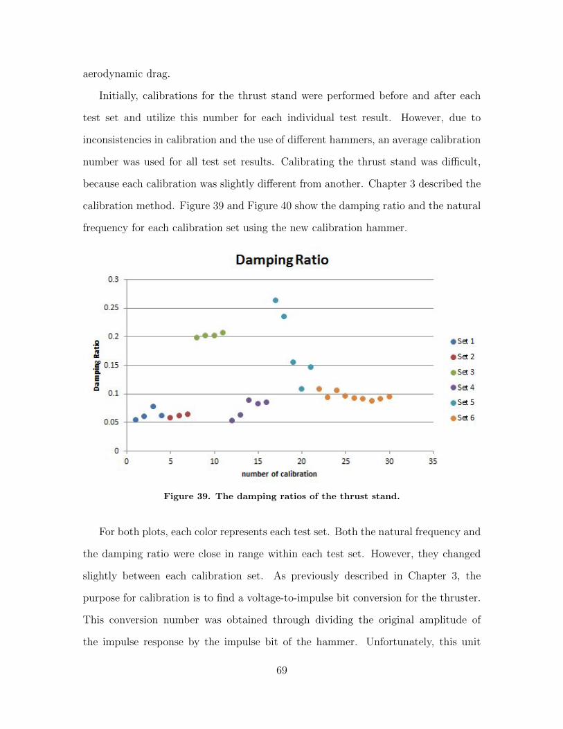
aerodynamic drag.

Initially, calibrations for the thrust stand were performed before and after each

test set and utilize this number for each individual test result. However, due to

inconsistencies in calibration and the use of different hammers, an average calibration

number was used for all test set results. Calibrating the thrust stand was difficult,

because each calibration was slightly different from another. Chapter 3 described the

calibration method. Figure 39 and Figure 40 show the damping ratio and the natural

frequency for each calibration set using the new calibration hammer.

Figure 39. The damping ratios of the thrust stand.

For both plots, each color represents each test set. Both the natural frequency and

the damping ratio were close in range within each test set. However, they changed

slightly between each calibration set. As previously described in Chapter 3, the

purpose for calibration is to find a voltage-to-impulse bit conversion for the thruster.

This conversion number was obtained through dividing the original amplitude of

the impulse response by the impulse bit of the hammer. Unfortunately, this unit

69

Figure 40. The natural frequencies of the thrust stand.

conversation number was different for each calibration strike. They ranged roughly

between 5 to 10 Volts per V/N-S. Figure 41 shows the difference in each calibration.

Figure 41. Unit impulse responses magnitude of the thrust stand.

70

The major inconsistency in calibration is uncertain because the calibration data

were too far apart. This was not expected. For nozzle 2 calibrations, the hammer

was struck approximately the same location as the small hammer. The distance ratio

between the thruster and the hammer was 0.52. In order to eliminate the distance

measurement and scaling error, the hammer strikes for the first two calibration sets

for nozzle 3 were located at equal distances to the thruster. Therefore, the distance

ratio between the thruster and the hammer was minimal. The last two calibration

sets for nozzle 3 were applied directly onto the thruster. This was the same location

where the thruster fires. It was assumed that the last two calibration sets were the

most accurate to the thruster response.

Since a wide range of calibration data exists, taking an average over all the data

would lead to inaccuracy. Therefore, the final unit conversion number was calculated

using only the average of the last calibration set, where the hammer input was applied

directly on the thruster. This method was chosen based on the assumption the thrust

stand response is consistent through all tests. The thrust stand had the same stiffness

during each test, and all the components, including the counterweights, had remained

constant. The only factor different was the location of the wire cable connecting the

thrust stand to the thruster and the slightly varying mass of the thruster due to

propellant consumption. Since the thruster was the only item taken on and off the

thrust stand between each test, the damping from the wires could cause a small

deviation in the response. Figure 39 indicates the damping from the last calibration

set was in the similar damping range as the other calibration sets.

Due to inconsistencies in calibration, this research has taken this error into account

in the upcoming performance criteria calculations. Performance criteria calculation

was based on the 6.26 V/N-S conversion number. Using a lower conversion number of

5/N-S will yield a 25% increase in impulse bit, specific impulse, and thrust coefficient.

71

Using a higher conversion number of 10 V/N-S will yield a 37% decrease in impulse

bit, specific impulse, and thrust coefficient.

4.2 Performance Analysis

This research consisted of testing the original nozzle and the three additional

nozzles at plenum pressure of 30 psia, 40 psia, and 45 psia at 3 x 10−4 torr. Table 4

displays the test conditions for this research. Test 1 through Test 10 were completed

while Test 11 and Test 12 were not completed due to malfunction of the thruster.

Each test consisted of 9 to 12 firings. The thruster was weighed before and after each

Table 4. Test conditions for the HYDROSTM thruster.

Original Nozzle Test 1 Test 2 Test 3

ε = 266 P1 (psia) 30 40 45

Pa (torr) 3 x 10−4 3 x 10−4 3 x 10−4

Nozzle 1 Test 4 Test 5 Test 6

ε = 55 P1 (psia) 30 40 45

Pa (torr) 3 x 10−4 3 x 10−4 3 x 10−4

Nozzle 2 Test 7 Test 8 Test 9

ε = 266 P1 (psia) 30 40 45

Pa (torr) 3 x 10−4 3 x 10−4 3 x 10−4

Nozzle 3 Test 10 Test 11 Test 12

ε = 22 P1 (psia) 30 40 45

Pa (torr) 3 x 10−4 3 x 10−4 3 x 10−4

72

test to determine the mass change. Three assumptions were applied to the tests: first,

the moment of inertia of the thrust stand remained constant throughout all test sets

due to only a small mass change in propellant; secondly, the manufacturing tolerance

in throat area was small and negligible; lastly, it was assumed nozzle contours had no

affect on the water electrolysis process or on combustion; therefore, mass-per-fire for

each plenum pressure was the same for all nozzle designs.

4.2.1 Impulse Bit.

Figure 42 illustrates the average impulse bit data of the four nozzles at various

plenum pressures. The error bars show the standard error of each test set. Error

Figure 42. Impulse bit data of the four nozzles.

73

method was analyzed in Chapter 3. The equation for Ibit is shown in Eq. (74),

Ibit =displacement

6.26(74)

where 6.26 is the calibration conversion number in V/N-S. All the raw impulse bit

data are located in Appendix A.

Figure 42 indicates as pressure increases, the impulse bit also increases. This is

expected because pressure is related to Reynolds number. An increase in Reynolds

number would increase the thrust coefficient. Since thrust is directly related to cham-

ber pressure and thrust coefficient, then chamber pressure also has a direct impact

on impulse bit. The higher pressure correlates to an increase in the mass expended.

As mass flow went up, the thrust coefficient also went up. Spisz et al.’s research had

also shown as Reynolds number increases, performance also increases [26].

The original nozzle, indicated in blue, did not follow this behavior. There is an

impulse bit drop between 40 and 45 psia. This drop was not expected. The original

nozzle data were inconclusive due to the separation of the nozzle flow. The images

of this separation are showed in the exhaust plume attachments section. In order to

provide a better understanding of the original nozzle, more data points at 40 and 45

psia are required.

Viscous effect varies depending on the Reynolds number range. For this research,

there is no accurate way to measure the Reynolds number and mass flow rate for each

pressure. Therefore, estimations were made using the ideal conditions from CEA. The

chamber pressures were unknown, because chamber pressure could decrease due to

pressure drop in the injector, or increase due to periods of combustion which are

closer to constant volume rather than constant pressure. Due to this reason, the

Reynolds number and mass flow rate calculations were based on the plenum pressure.

Although the Reynolds number changed as the nozzle expanded and mass flow rate

74

decreased, the estimations were made at the throat. These Reynolds numbers were

used to compare with Spisz et al.’s research, since their data were correlated in terms

of throat Reynolds number as well. Table 5 shows the CEA estimated Reynolds

number and mass flow rate for each pressure at the throat. Chamber pressure changes

during the pulse, it drops as the mass is expended. The average pulse duration was

Table 5. The estimated throat conditions.

Pressure (psia) m (kg/s) Re

30 1.21 x 10−4 1243

40 1.61 x 10−4 1636

45 1.81 x 10−4 1831

approximately in the range between 0.2 to 1 second. Using this range with the mass

per fire measured from experiment, the actual mean mass flow was on the order of

10−5; this means the actual Reynolds numbers were expected to have a lower value

than the CEA Reynolds numbers. In addition, CEA calculations were based on steady

state operation. Due to the pulsed nature of the thruster, the Reynolds numbers were

lower than calculated, however, the exact range is unknown.

By comparing nozzle 1 and nozzle 2, nozzle 1 with a 55 expansion ratio has a

higher impulse bit than nozzle 2 with a 266 expansion ratio at 40 psia. The results

at 40 psia corresponded with the Spisz et al.’s low Reynolds number research. Their

research indicated for low Reynolds numbers (below 10,000), the benefit of having

a larger expansion ratio might not exceed the increase in viscous effects, due to the

added surface area [26]. By observing Figure 42, this conclusion only held true at 40

psia and not at the lower (30 psia) and higher (45 psia) pressure.

At 30 psia plenum pressure, the data points for the nozzles were very close to-

gether. As shown in Table 5, from 45 psia to 30 psia, Reynolds number drops from

75

around 1800 to 1200 and possibly lower due to the pulse condition. Due to viscous

effects dominating the flow at low Reynolds numbers, the data showed nozzle contour

and expansion ratio have little influence on performance compared to the 40 and 45

Psia data points. Since data for nozzle 3 at 40 and 45 psia were not captured, it is

difficult to conclude the behavior at those pressures. However, nozzle 3 performance

at 30 psia was higher, and this could suggest a similar performance range to nozzle

1.

At 45 psia, nozzle 1 performance is slightly higher than nozzle 2, however, the same

argument might not hold true at 45 psia due to the small overlap in error. There

is a maximum impulse bit value this system could obtain. At 45 psia, the system is

getting closer to this limit, thus, the nozzle contour has less effects on performance.

The smaller expansion ratio has a closer performance with the higher expansion ratio

at 45 psia compared to 40 psia. Another reason was because as Reynolds number

increases, viscous effects also decreases. At 45 psia, the negative effects of having

additional surface area for the nozzle 2 might began to decrease.

In conclusion, impulse bit increases with increasing plenum pressure because

Reynolds numbers increases with pressure and there is an increase in gross mass

with pressures. Original nozzle behavior was inconclusive due to early flow separa-

tion. More data would be required to draw further conclusions. Performance between

nozzle 1 and nozzle 2 at the lower and higher pressures indicated this thruster could

obtain a minimum and maximum impulse bit regardless of the expansion ratio of

the nozzle. At 30 psia, the nozzle was dominated by viscous boundary layers. At

40 psia, nozzle 1 with the smaller expansion ratio and less surface area had a better

performance than nozzle 2 due to less viscous effects. At 45 psia, different nozzles

performance were closer together because the system was reaching its maximum value

on the performance curve. Thrust coefficient goes up dramatically for the lower area

76

ratios, but it only rises up slightly as area ratios increase. Impulse bit is more depen-

dent on chamber pressures than other factors, such as expansion ratios.

4.2.2 Specific Impulse.

Specific impulse, Isp, is a way to measure the efficiency of the system. It is the

impulse delivered per unit of propellant. It is derived from the impulse bit shown in

Eq. (75),

Isp =

∑Ibit

∆mgo(75)

where ∆m is the change of mass in each test set. The specific impulse value could

directly applied to a spacecraft to calculate delta V, which is important for space

missions to determine the possible maneuvers. The raw data for specific impulse and

thrust coefficient are located in Appendix B.

Figure 43 displays the specific impulse data of the four nozzles for this research.

Specific impulse performance at 30 psia was similar to the impulse bit data. Nozzle 3

has a slightly higher average impulse bit compared to the rest of the nozzles. However,

when looking at efficiency, nozzle 3 has performance similar to the other nozzles at

30 psia. The same trend was indicated in this specific impulse plot, where viscous

effects dominate at the low Reynolds number. Nozzle contour and expansion ratio

have a minor performance influence at 30 psia.

At 40 psia, nozzle 1 was expected to have a higher Isp performance compared to

nozzle 2 based on the impulse bit data. However, this behavior did not appear in the

Isp data due to a large error in measurement. If the Isp error bars were as small as

the impulse bit error bars, then the same trend would appear. Between 40 and 45

psia, there was also a slight drop in performance for nozzle 1, but this is insignificant

because it was also within the measurmement errors. The data between 40 and 45

psia were not expected to be far apart because the difference in performance between

77

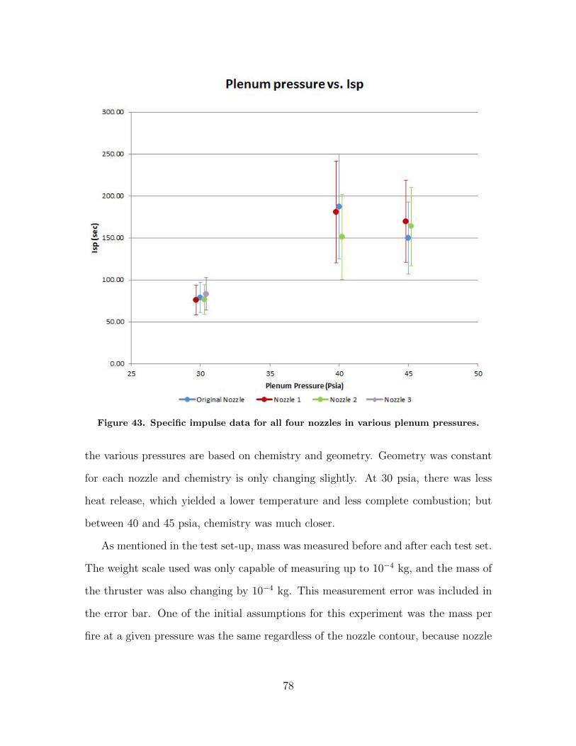
Figure 43. Specific impulse data for all four nozzles in various plenum pressures.

the various pressures are based on chemistry and geometry. Geometry was constant

for each nozzle and chemistry is only changing slightly. At 30 psia, there was less

heat release, which yielded a lower temperature and less complete combustion; but

between 40 and 45 psia, chemistry was much closer.

As mentioned in the test set-up, mass was measured before and after each test set.

The weight scale used was only capable of measuring up to 10−4 kg, and the mass of

the thruster was also changing by 10−4 kg. This measurement error was included in

the error bar. One of the initial assumptions for this experiment was the mass per

fire at a given pressure was the same regardless of the nozzle contour, because nozzle

78

design should not affect the water electrolysis and combustion process. However,

test data indicated differently for each nozzle design due to the mass measurement

error. Therefore, in order to minimize this error, an average mass per fire for each

plenum pressure was applied to all nozzle data. The average mass for each pressure

was calculated using Eq. (76),

Average mass per fire =

4∑i=1

∆mi

4∑i=1

ni

(76)

where 4 represents the sum of all four nozzle sets and n is the number of fire. The over-

all change of mass for Isp calculation for each test set was calculated using Eq. (77),

∆m = mn (77)

where m is the average mass per fire.

Table 6. The average mass per fire for various plenum pressures.

Pressure (Psia) Average mass per fire (kg)

30 3.65 x 10−5

40 2.57 x 10−5

45 3.09 x 10−5

The average mass per fire for each pressure is shown in Table 6. As pressure

increases, the mass required to fire should also increase. However, Table 6 does not

indicate the same result due to the measurement error mentioned above. In order to

obtain more accurate mass per fire data, more data points are required. In addition,

the 30 psia tests were first performed after receiving the thruster back from nozzle

79

replacement. The first tests might consume more propellant when first run in vacuum.

The mass data for this research is included in Appendix C.

In order to obtain a better understanding of what the mass per fire for the various

pressures were, mass estimations were calculated using the ideal gas law. The ideal

gas law is shown in Eq. (78),

m =PVM

RT(78)

where m is mass, M is the molar mass of the gas, P is the pressure of the gas, V

is the gas volume, R is the universal gas constant, and T is the temperature of the

gas, which was assumed to be room temperature at 300 K. The mass values from

ideal gas law are the expected values and the mass per fire was expected to vary

linearly with plenum pressures. The equation was calculated separately at 30, 40,

and 45 psia, for gaseous hydrogen and oxygen. Hydrogen and oxygen volume were

based on the gas tanks volume, provided by TUI, which are 12.9 cm3 and 6.6 cm3,

respectively. Figure 44 shows the updated mass per fire along with the experimental

data. Figure 44 indicates at 40 and 45 psia, the average mass per fire measured

were very close compared to the ideal gas law calculation. On the other hand, the

measured average value at 30 psia was too high.

Figure 45 shows the expected Isp trend with the mass corrections. The projected

nozzle 3 data for 40 and 45 psia are also plotted to show a complete data set. Nozzle

3 was suggested to have the same or higher Isp as nozzle 1, based on its behavior at 30

Psia. With the new mass distribution, the trend between 40 to 45 psia was improved.

Even though, this trend is not as linear as expected, the drop of performance between

40 and 45 psia appeared with the original data, shown in Figure 43, was dissolved.

In addition, the measured Isp values at 30 psia jumped from the 75 second range to

140 second range by using the ideal gas law mass. This was a better representation

on Isp because performance at 30 psia should not have a 50% drop compared to 40

80

Figure 44. The comparison between the experimental average mass values and theideal gas law mass values.

Figure 45. New Isp data with updated mass values.

81

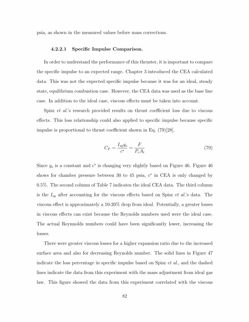
psia, as shown in the measured values before mass corrections.

4.2.2.1 Specific Impulse Comparison.

In order to understand the performance of this thruster, it is important to compare

the specific impulse to an expected range. Chapter 3 introduced the CEA calculated

data. This was not the expected specific impulse because it was for an ideal, steady

state, equilibrium combustion case. However, the CEA data was used as the base line

case. In addition to the ideal case, viscous effects must be taken into account.

Spisz et al.’s research provided results on thrust coefficient loss due to viscous

effects. This loss relationship could also applied to specific impulse because specific

impulse is proportional to thrust coefficient shown in Eq. (79)[28].

CF =Ispgoc∗

=F

PcAt(79)

Since go is a constant and c∗ is changing very slightly based on Figure 46. Figure 46

shows for chamber pressure between 30 to 45 psia, c∗ in CEA is only changed by

0.5%. The second column of Table 7 indicates the ideal CEA data. The third column

is the Isp after accounting for the viscous effects based on Spisz et al.’s data. The

viscous effect is approximately a 10-20% drop from ideal. Potentially, a greater losses

in viscous effects can exist because the Reynolds numbers used were the ideal case.

The actual Reynnolds numbers could have been significantly lower, increasing the

losses.

There were greater viscous losses for a higher expansion ratio due to the increased

surface area and also for decreasing Reynolds number. The solid lines in Figure 47

indicate the loss percentage in specific impulse based on Spisz et al., and the dashed

lines indicate the data from this experiment with the mass adjustment from ideal gas

law. This figure showed the data from this experiment correlated with the viscous

82

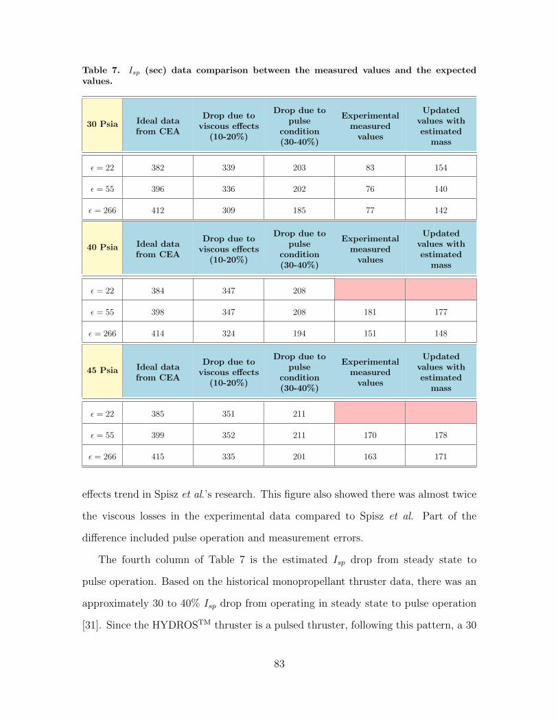
Table 7. Isp (sec) data comparison between the measured values and the expectedvalues.

30 Psia Ideal datafrom CEA

Drop due toviscous effects

(10-20%)

Drop due topulse

condition(30-40%)

Experimentalmeasured

values

Updatedvalues withestimated

mass

ε = 22 382 339 203 83 154

ε = 55 396 336 202 76 140

ε = 266 412 309 185 77 142

40 Psia Ideal datafrom CEA

Drop due toviscous effects

(10-20%)

Drop due topulse

condition(30-40%)

Experimentalmeasured

values

Updatedvalues withestimated

mass

ε = 22 384 347 208

ε = 55 398 347 208 181 177

ε = 266 414 324 194 151 148

45 Psia Ideal datafrom CEA

Drop due toviscous effects

(10-20%)

Drop due topulse

condition(30-40%)

Experimentalmeasured

values

Updatedvalues withestimated

mass

ε = 22 385 351 211

ε = 55 399 352 211 170 178

ε = 266 415 335 201 163 171

effects trend in Spisz et al.’s research. This figure also showed there was almost twice

the viscous losses in the experimental data compared to Spisz et al. Part of the

difference included pulse operation and measurement errors.

The fourth column of Table 7 is the estimated Isp drop from steady state to

pulse operation. Based on the historical monopropellant thruster data, there was an

approximately 30 to 40% Isp drop from operating in steady state to pulse operation

[31]. Since the HYDROSTM thruster is a pulsed thruster, following this pattern, a 30

83

Figure 46. Characteristics velocity values in CEA.

to 40% drop in Isp was expected as well and potentially more. Potential performance

losses might exist due to the chamber pressure rising and then falling as the tank

empties. Therefore, the Isp number in Column 4 is the expected Isp range, after taking

viscous effects and pulse operation into account. Column 5 illustrates the measured Isp

values from this research. The measured values were lower than the expected values.

The differences could be attributed to incomplete combustion leading to reduced c∗,

error from mass measurement, and error from thrust stand calibration. The last

column shows the Isp value using the adjusted ideal gas law’s mass for comparison.

At 30 psia, there is a gain in Isp due to the decrease in mass expended. This is a better

representation of what happened because performance between the various pressures

is expected to be within a close range from each other, similar to the ideal CEA data.

The CEA data from column 2 showed a small change in Isp between each pressure.

The percentage difference between the expected Isp and the measured Isp is shown

84

Figure 47. Loss percentage in specific impulse and thrust coefficient based on Spisz etal.

in Figure 48. The expected values in Figure 48 had taken both viscous effects and

pulse condition into account. The percentage drop between the experimental values

and the expected values, as well as the percentage drop between the new estimated

values using the ideal gas law mass and the expected values, were both showed in

Figure 48. Before the mass adjustment, there was an approximately 60% drop in

performance at 30 psia. This loss percentage got reduced down to about 25% with

the new mass. The loss percentage for both cases were similar at 40 and 45 psia, as

well as at the different expansion ratios. They were all between 15-25%. The purpose

of Figure 48 is to show what the difference is between the expected values from

previous research, which included viscous effects losses from a steady-state operation

85

Figure 48. Loss percentage in performance between the expected values and the mea-sured values.

studies and pulse condition losses from larger scale thrusters, to the measured values

for a small scale pulsed chemical thruster.

Another important relationship to look at is the overall losses starting from the

ideal CEA values all the way down to the measured values. The percentage of the

overall losses is shown in Figure 49. The dotted lines in Figure 49 were the ideal losses,

which only included the 10-20% drop from viscous effects and 40% drop from pulse

operation. The lines showed there were greater losses with increasing expansion ratio

and increasing pressure. The loss differences between various pressures were minimal,

only a few percentage drop from each one another. At 30 psia, loss percentage dropped

from about 80% down to about 65% with the new mass adjustment. The data at 40

and 45 psia followed similar results as the ideal losses. Looking at performance losses,

there were higher overall losses and viscous losses with the increase in expansion ratio.

86

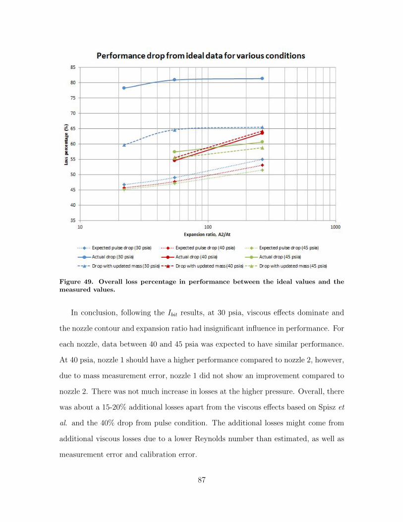
Figure 49. Overall loss percentage in performance between the ideal values and themeasured values.

In conclusion, following the Ibit results, at 30 psia, viscous effects dominate and

the nozzle contour and expansion ratio had insignificant influence in performance. For

each nozzle, data between 40 and 45 psia was expected to have similar performance.

At 40 psia, nozzle 1 should have a higher performance compared to nozzle 2, however,

due to mass measurement error, nozzle 1 did not show an improvement compared to

nozzle 2. There was not much increase in losses at the higher pressure. Overall, there

was about a 15-20% additional losses apart from the viscous effects based on Spisz et

al. and the 40% drop from pulse condition. The additional losses might come from

additional viscous losses due to a lower Reynolds number than estimated, as well as

measurement error and calibration error.

87

4.2.3 Thrust Coefficient.

Thrust coefficient, CF , is another way to look at the efficiency of the system. Since

the thrust of this system is unknown, the thrust coefficient data were calculated using

specific impulse showed in Eq. (79). Figure 50 displayed the thrust coefficient result

Figure 50. The thrust coefficient data of the four nozzles at various plenum pressure.

of the four nozzles at various plenum pressures. The data trend between thrust

coefficient and specific impulse are similar because they are related to one another.

The two are not directly proportional due to the small change in c∗. At 30 psia,

all four nozzles have similar performance, because viscous effects dominate in low

Reynolds number flows. Between 40 and 45 psia, nozzle 1, with a smaller expansion

ratio (ε = 55), has a slightly higher performance in CF than nozzle 2 (ε = 266) without

taking error into account. However, taking into account of the error bars, the two

88

nozzles were indicated to have a similar performance. Data at 40 psia also displayed

similar trends to 45 psia.

As previously explained, performance between the various pressures should not

have a significant difference. However, comparing the data between 30 psia and 40

psia in Figure 50, it showed an approximately 50% drop in thrust coefficent. This

was mainly caused by the high average mass per fire at 30 psia. Using the ideal gas

law mass calculated earlier, Figure 51 illustrates the expected thrust coefficient trend

after the adjustments were made in mass per fire. The projected nozzle 3 data at 40

Figure 51. The updated thrust coefficient data with mass adjustment.

and 45 psia were also plotted for completeness. With this estimated mass, there was

only a 20% drop in performance from 40 to 30 psia. The data for all three pressures

were much closer in range with the mass correction.

89

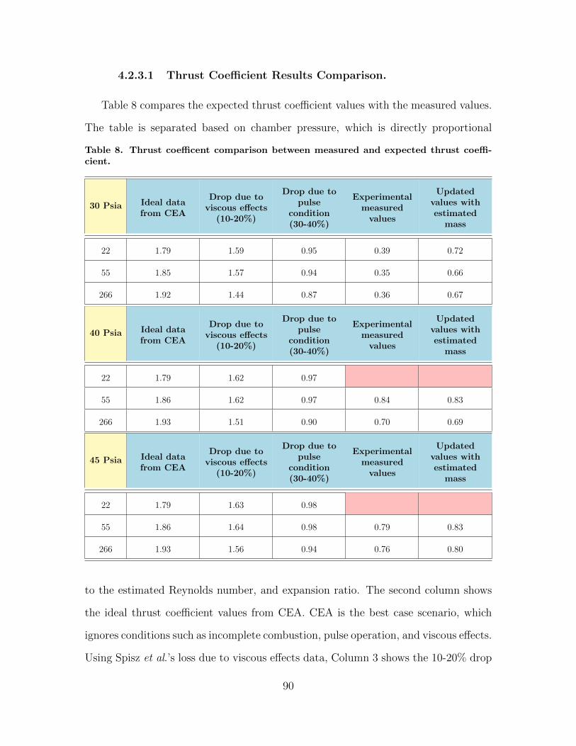
4.2.3.1 Thrust Coefficient Results Comparison.

Table 8 compares the expected thrust coefficient values with the measured values.

The table is separated based on chamber pressure, which is directly proportional

Table 8. Thrust coefficent comparison between measured and expected thrust coeffi-cient.

30 Psia Ideal datafrom CEA

Drop due toviscous effects

(10-20%)

Drop due topulse

condition(30-40%)

Experimentalmeasured

values

Updatedvalues withestimated

mass

22 1.79 1.59 0.95 0.39 0.72

55 1.85 1.57 0.94 0.35 0.66

266 1.92 1.44 0.87 0.36 0.67

40 Psia Ideal datafrom CEA

Drop due toviscous effects

(10-20%)

Drop due topulse

condition(30-40%)

Experimentalmeasured

values

Updatedvalues withestimated

mass

22 1.79 1.62 0.97

55 1.86 1.62 0.97 0.84 0.83

266 1.93 1.51 0.90 0.70 0.69

45 Psia Ideal datafrom CEA

Drop due toviscous effects

(10-20%)

Drop due topulse

condition(30-40%)

Experimentalmeasured

values

Updatedvalues withestimated

mass

22 1.79 1.63 0.98

55 1.86 1.64 0.98 0.79 0.83

266 1.93 1.56 0.94 0.76 0.80

to the estimated Reynolds number, and expansion ratio. The second column shows

the ideal thrust coefficient values from CEA. CEA is the best case scenario, which

ignores conditions such as incomplete combustion, pulse operation, and viscous effects.

Using Spisz et al.’s loss due to viscous effects data, Column 3 shows the 10-20% drop

90

in thrust coefficient performance. There is a greater loss for the higher expansion

ratio nozzles, as well as at lower pressure. Column 4 indicates the expected thrust

coefficient after the 30 to 40% drop from steady state to pulse operation, largely due

to a decrese in average pressure when compared to steady thrust profiles. Column 5

is the measured values. Compared to Column 4, Column 5 is lower, because there

are additional losses due to incomplete combustion, mass measurement error, and

thrust stand calibration error. There is a larger difference in 30 psia, because for the

CEA ideal case, chamber pressure variation has low impact on the calculated CF in

vacuum as shown in Column 2. However, in the measured values, there was a close

to 50% jump in performance between 30 and 40 psia due to mass measurement error.

With the estimated mass from ideal gas law showed in column 6, the data between

the different pressures were within 2-3% of each other, similar to the relationship in

CEA data. The CF values in Column 5 and Column 6 were the worse case values

because the thrust coefficient calculations were based on an ideal c∗ value. This c∗

value would only decrease. And thrust coefficient increases with decreasing c∗ for a

fixed specific impulse value.

The viscous losses percentage and the overall losses percentage data between the

expected and the measured values were the same as the data showed in Figure 48

and Figure 49, since Isp and CF are proportional with only a slight change in c∗.

Figure 52 compares the trend between Spisz et al. data and experimental data

from this research. Spisz et al.’s data indicated the thrust coefficient data for steady

state operation in terms of expansion ratio and Reynolds number. This data was

for gamma = 1.4 expansion and for this research, gamma was closer to 1.3. The

experimental thrust coefficient data in Figure 52 included the mass adjustment from

ideal gas law and the projected nozzle 3 performance at 40 and 45 psia.

The two sets of data both showed a performance decrease with an increase in

91

Figure 52. Thrust coefficient trend comparison with Spisz et al. research data.

expansion ratio and decrease in Reynolds number. However, the slopes of the curve

were decreasing more sharply than for Spisz et al. data. The difference might come

from the pulse condition of this thruster. Figure 52 showed at 30 psia, expansion ratio

has less influence in performance and at 45 psia, the performance of the thruster was

getting closer to the maximum values on the performance curve. Therefore, a decrease

in expansion ratio did not provide a major improvement in performance compared

to 40 psia because the performance curve was leveling off at the higher pressure.

In addition, the data from Spisz et al. were based on different Reynolds numbers.

The Reynolds numbers were chosen for comparison based on CEA calculations. The

experimental data could have a lower and decreasing Reynolds number due to the

decreasing mass flow caused by pulse operation. And Spisz et al.’s research Reynolds

numbers were constant due to steady state operation. Therefore, at 30 psia, viscous

92

effects for experimental data were larger and expansion ratio became less significant

compared to Spisz et al 30 psia data.

4.3 Exhaust Plume Attachments

Nozzle exit flow attachment is critical for system performance. Flow separation

in the nozzle can reduce nozzle efficiency, thus decreasing system performance. In

the summer of 2014, high speed images of the original factory nozzle exhaust were

captured. These images are shown in Figure 53 [14]. The high speed images indicated

there was flow separation with this bell nozzle. The exhaust flow is not attached to

the nozzle wall. The efficiency of the system is decreased due to this separation, and

new nozzle design is needed to improve system performance.

Nozzle 1 high speed images are showed in Figure 54. Nozzle 2 high speed images

are shown in Figure 55, and nozzle 3 images are shown in Figure 56. The exhaust

plume between the original nozzle and the new nozzles did not change much, but the

new nozzles were shaped to better match the exhaust. Using the images, exhaust

angles were calculated to quantify improvements. These were estimated angles be-

cause the measurements were only based on the images captured. The exhaust plume

angles were roughly between 14 to 18-degree.

Based on the new nozzle images and the calculated angles, the exhaust plume

aligned closer to the 15-degree nozzle contour compared to the 37-degree bell nozzle.

Flow separation at the exit plane was difficult to measured. For the original nozzle,

there was about a 5.6 mm separation distance. However, due to the similar angle be-

tween new nozzle contour and the exhaust plume, there were only minimal separation

distance for the conical nozzles. These findings indicated changing the nozzle design

to a 15-degree conical nozzle can help improve the flow separation problem, as well as

help improve the nozzle efficiency. The fire duration for this thruster is unmeasurable

93

Figure 53. High speed images of factory nozzle: Exposure time of 264 ms (30 fps) [14].

by the means at hand. However, by observing the exposure time of the high speed

images, the images showed an inconsistency in fire duration pattern. Based on the

images, it can concluded the new nozzles helped to improve systems efficiency. This

efficiency might not represented well in the Isp and CF data due to the large error in

measurement.

94

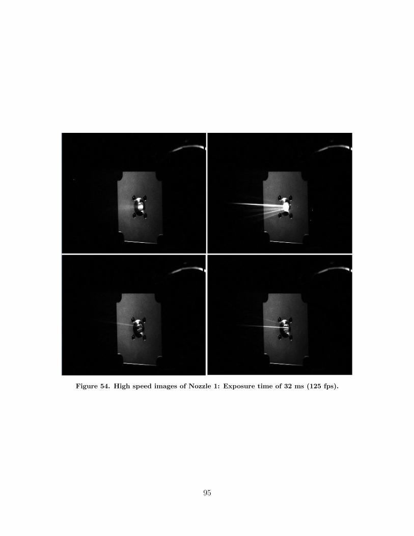
Figure 54. High speed images of Nozzle 1: Exposure time of 32 ms (125 fps).

95

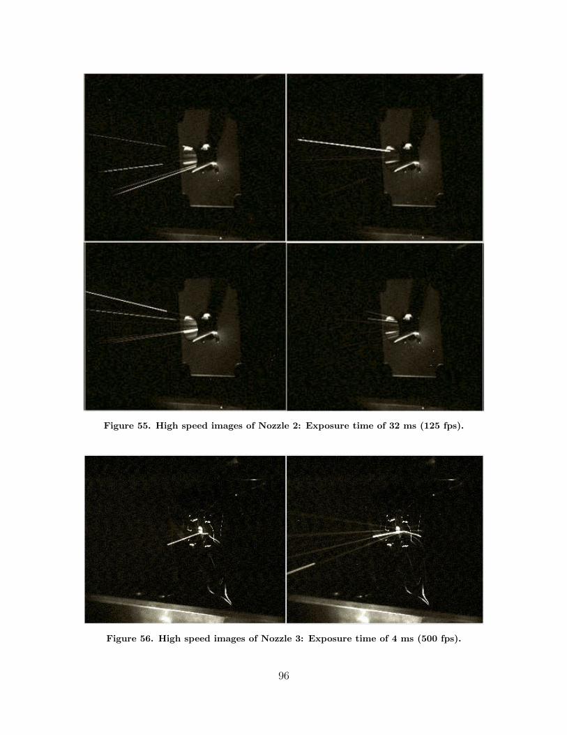
Figure 55. High speed images of Nozzle 2: Exposure time of 32 ms (125 fps).

Figure 56. High speed images of Nozzle 3: Exposure time of 4 ms (500 fps).

96

V. Conclusions and Future Work

In chapter 1, a list of research objectives was established. These objectives served

as the guidelines throughout this research. The goal for this research is to under-

stand how different nozzle contours affect performance and efficiency in small pulsed

chemical thrusters. Each objective leads the research closer to the research goal. This

concluding chapter will review those objectives and evaluate if the research goal was

met. In addition, this chapter will also summarize the result for this research, and

recommendations for future work.

5.1 Research Objectives Review

The five research objectives are as follows:

1. Design nozzles using a nominal two-dimensional conical geometry to improve

the specific impulse of the thruster and verify results by using the experimental

impulse bit data to calculate specific impulse.

2. For each nozzle design, experimentally measure performance criteria such as

impulse bits, thrust coefficient as a function of the plenum pressure envelope at

30, 40, and 45 psia, in vacuum using a torsional balance thrust stand.

3. Determine nozzle performance at various plenum pressures and expansion ratios

by comparing thrust coefficient.

4. Examine viscous effects on nozzles by comparing experimental data with ideal

CEA data and previous research data.

5. Determine nozzle efficiency improvement by comparing the exhaust flow attach-

ment points relative to the nozzle using images from a high-speed camera.

97

A total of 10 test sets were conducted at 3 x 10−4 Torr. Each test set consisted of

9 to 12 firings. The test sets included firing the original nozzle, nozzle 1, and nozzle 2

at 30, 40, and 45 psia plenum pressure and nozzle 3 at 30 psia plenum pressure. Due

to thruster malfunctions, testing for nozzle 3 was not conducted at 40 and 45 psia

plenum pressure. The original nozzle is a bell nozzle with a 266 expansion ratio and a

short length that does not follow the nominal two dimensional MOC. Nozzle 1, 2, and

3 are 15-degree conical nozzles with a 55, 266, and 22 expansion ratio, respectively.

Objective 1 was partially satisfied. The three additional nozzles were designed as

15 degrees conical nozzles based on previous research indicating that bell nozzles were

contraindicated at low Reynolds numbers, and were successfully manufactured at the

AFIT machine shop. This objective was only partially satisfied due to mass mea-

surement error and unreliable data sets for the original nozzle, therefore, a conclusion

toward the new designs performance is not certain. Even though there was strange

behavior in the original nozzle due to flow separation, impulse bit data showed an

improvement in impulse bit performance using the new nozzle designs at the 45 psia

plenum pressure. Because data from the original nozzle is not reliable, a conclusion

of whether impulse bit performance has been improved at 30 and 40 psia cannot be

made. However, overall, the maximum nozzle 1 and 2 impulse bits are higher than

the maximum original nozzle impulse bit. For specific impulse, there is a larger error

bar due to the mass per fire uncertainty. The original nozzle and nozzle 1 both had

similar performances in specific impulse.

Objective 2 was also partially satisfied because hardware malfunctions prevented

measurement of performance with nozzle 3 at 40 and 45 psia plenum pressure. The

rest of the experiments were successfully measured using a torsional balance thrust

stand.

Objective 3 was satisfied. Experimental data for thrust coefficient were calculated

98

and shown in terms of expansion ratio and plenum pressure. The results showed

low plenum pressure performance for different expansion ratios were similar because

viscous effects dominate. At 40 psia, the results showed a higher performance with the

smaller expansion ratio compared to the higher expansion ratio because the increase

in area ratio was not enough to overcome the additional viscous effects caused by the

increased surface area. At 45 psia, expansion ratio had less affects in performance as

well because the system was reaching toward the maximum value on the performance

curve. The relationship between expansion ratio and performance began to level off

at the high pressure.

Objective 4 was also satisfied. Data was compared and analyzed in chapter 4.

Specific impulse and thrust coefficient data were compared to the expected data.

The expected data started off with the ideal CEA data. Then, 10 to 20% drop due to

viscous effects based on Spisz et al. data [26] and 30 to 40% drop from steady state

to pulse operation based on historical data were deducted from the ideal CEA data.

The percentage loss between the experimental value and the expected value showed

there was a greater loss at the lower pressure. For the higher pressure, loss percentage

were similar between 40 and 45 psia. In addition, different expansion ratios also had

a similar loss between the expected and measured value. Between the ideal data

and the measured data, results showed an increase in loss percentage with increasing

expansion ratio. At 40 and 45 psia, losses were also similar at each expansion ratio.

Objective 5 was satisfied. High speed images of each nozzle were successfully

captured. High speed images of the three nozzle designs have shown an improvement

in exhaust plume flow attachment compared to the original nozzle high speed images

based on the exhaust plume angles. The exhaust angles were around 14-18-degree,

which is closer to the 15-degree conical nozzle contour. The exit flow was more aligned

with the new nozzle contour. This showed redesigning the nozzle using a 15-degree

99

conical nozzle can improve the flow separation problems and also improve nozzle

efficiency.

5.2 Recommendation and Future work

The HYDROSTM thruster is a 1U chemical pulsed thruster. This thruster operates

in low Reynolds number and low mass flow rate conditions. It also has incomplete

combustion, and non-steady state flow. Previous research conducted on low thrust

and low Reynolds number thrusters were for steady state operation. With this re-

search, knowledge in behavior and performance for a chemical pulse thruster was

gained through comparing with the research from Spisz et al.

The original nozzle is not recommended for this thruster because experimental

data and high speed images suggested this nozzle has early flow separation. It is

not recommended to use a system because flow separation reduces nozzle efficiency.

Nozzle 2 with a high expansion ratio of 266 and a length that extended out of the 1U

configuration is also not recommended. The experimental result showed no benefit

with the added length. Nozzle 1 and Nozzle 3 showed the best performance behavior

out of the four nozzles. With similar behavior, nozzle 3 would be recommended over

nozzle 1 because with the smaller expansion ratio, using nozzle 3 would reduce the

weight and size of the 1U thruster. Reduced size and mass is beneficial for a volume

and mass constrained CubeSat. By switching from a 55 expansion ratio to a 22

expansion ratio nozzle, the reduced length could increase the fuel tank by 64%.

5.2.1 Torsional Balance Thrust Stand.

The torsional balance thrust stand was designed and built for the HYDROSTM

thruster by Tethers Unlimited, Inc. Thrust stand selection for this thruster was dif-

ficult due to the short pulse condition. The thrust stand must be able to capture

100

the natural frequency of the response, as well as treat the thruster response as an

impulse. The thrust stand for this research was a new design and it requires further

improvements. This research was not able to find a consistent calibration for this

thrust stand. Further investigation is required to determine why the thrust stand

behavior is inconsistent. A new calibration method might be necessary. In addition,

it was difficult to see if the swinging arm was absolutely parallel to the linear displace-

ment sensor. An electronically controlled level adjuster and LDS adjuster should be

added to the thrust stand to allow adjustments during vacuum testing.

5.2.2 The water electrolysis thruster.

The nozzle designs did not significantly improve the thrust coefficient or the spe-

cific impulse of the thruster as mentioned above in objective 1. A better weight scale

is needed to reduce mass measurement error. Using the new nozzle design is recom-

mended because it reduces flow separation. However, it did not change the range of

specific impulse. Due to the pulsed nature of this thruster, this system might not

follow a traditional method of nozzle design. A set of rules in nozzle design might

not exist for a low thrust, low Reynolds number, and incomplete combustion pulsed

chemical thruster. Recommendations would be to continue testing with different noz-

zle designs to find one that could improve the specific impulse and thrust coefficient

of the system. In order to make a significant improvement in performance for this

system, only changing the nozzle is not enough. There exists a limit on how much the

nozzle could improve the system. Apart from nozzle designs, it is possible to redesign

the thruster chamber length to accommodate the residence time and chemical time

to improve combustion efficiency. This could help with the incomplete combustion

problem. Lastly, the size of the H2 and O2 tank could also be increased to produce a

longer pulse. However, due to CubeSats sizing constraints, trade offs are required in

101

order to improve system performance. Increasing pulse time and increasing system

performance might require the thruster to extend out of its 1U configuration.

102

Appendix A. Impulse Bit Data

This appendix displayed the raw impulse bit data in voltage displacement prior

using the calibration conversion number. These data are the amplitude of the thrust

stand impulse response. Table 14 is for the original nozzle separated by different

plenum pressures. Table 10 is for nozzle 1, Table 11 is for nozzle 2, and Table 12 is

for nozzle 3.

103

Table 9. Original Nozzle Raw Data (V)

30 Psia 40 Psia 45 Psia

1 0.161 0.386 0.287

2 0.179 0.330 0.368

3 0.164 0.336 0.342

4 0.178 0.262 0.266

5 0.183 0.287 0.257

6 0.176 0.286 0.271

7 0.169 0.285 0.266

8 0.190 0.304 0.276

9 0.166 0.284 0.269

10 0.190 0.288 0.277

11 0.178 0.293 0.271

12 0.178 0.292 0.262

13 0.284

14 0.273

15 0.272

104

Table 10. Nozzle 1 Raw Data (V)

30 Psia 40 Psia 45 Psia

1 0.237 0.316 0.379

2 0.143 0.297 0.340

3 0.165 0.268 0.296

4 0.144 0.288 0.321

5 0.161 0.281 0.309

6 0.175 0.317 0.321

7 0.158 0.274 0.311

8 0.153 0.269 0.297

9 0.161 0.272 0.307

10 0.185 0.267 0.327

11 0.166 0.288 0.326

12 0.183 0.293 0.328

105

Table 11. Nozzle 2 Raw Data (V)

30 Psia 40 Psia 45 Psia

1 0.181 0.241 0.327

2 0.167 0.246 0.294

3 0.168 0.242 0.319

4 0.157 0.213 0.280

5 0.195 0.268 0.346

6 0.163 0.229 0.308

7 0.172 0.228 0.341

8 0.162 0.295

9 0.178 0.277

10 0.310

11 0.316

12 0.312

13 0.299

106

Table 12. Nozzle 3 Raw Data (V)

30 Psia

1 0.183

2 0.216

3 0.179

4 0.154

5 0.255

6 0.261

7 0.169

8 0.159

9 0.168

10 0.168

11 0.165

12 0.162

13 0.180

107

Appendix B. Specific Impulse and Thrust Coefficient Data

Table 14 displayed the Isp and CF data. Column 2 and Column 4 are the higher

and lower Isp values from error propagation. Column 5 and Column 7 are the higher

and lower CF values from error propagation.

Table 13. Isp data for the four nozzles.

Pressure (psia) (-) Isp(sec) (+) (-) CF (+)

Original Nozzle

30 60.66 78.69 96.72 0.28 0.37 0.45

40 124.55 186.99 249.43 0.58 0.87 1.16

45 106.36 149.19 192.02 0.49 0.69 0.89

Nozzle 1

30 58.08 75.68 93.28 0.27 0.35 0.44

40 120.39 180.76 241.13 0.56 0.84 1.12

45 121.16 169.88 218.59 0.56 0.79 1.02

Nozzle 2

30 59.13 76.77 94.40 0.28 0.36 0.44

40 100.46 150.95 201.43 0.47 0.70 0.94

45 116.63 163.42 210.21 0.54 0.76 0.98

Nozzle 3

30 63.68 83.19 102.71 0.30 0.39 0.48

108

Appendix C. Mass Per Fire Data

Table 14 displayed the mass data per each test set and the average mass per each

pressure.

109

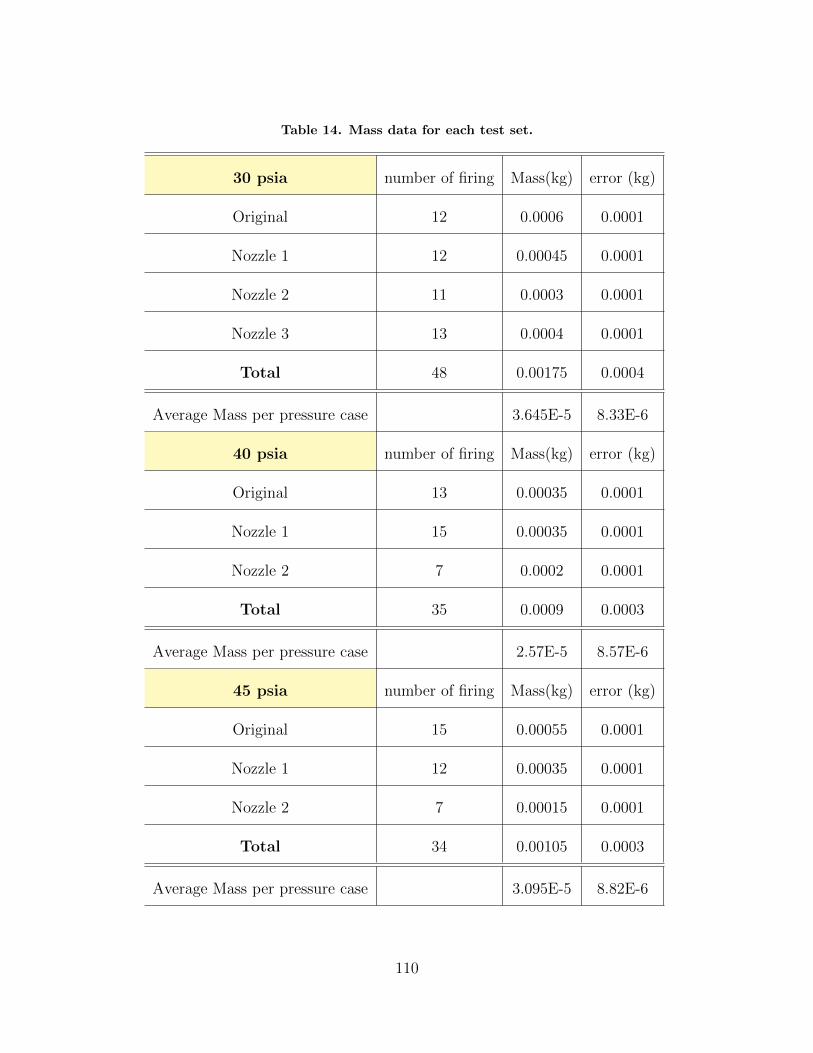
Table 14. Mass data for each test set.

30 psia number of firing Mass(kg) error (kg)

Original 12 0.0006 0.0001

Nozzle 1 12 0.00045 0.0001

Nozzle 2 11 0.0003 0.0001

Nozzle 3 13 0.0004 0.0001

Total 48 0.00175 0.0004

Average Mass per pressure case 3.645E-5 8.33E-6

40 psia number of firing Mass(kg) error (kg)

Original 13 0.00035 0.0001

Nozzle 1 15 0.00035 0.0001

Nozzle 2 7 0.0002 0.0001

Total 35 0.0009 0.0003

Average Mass per pressure case 2.57E-5 8.57E-6

45 psia number of firing Mass(kg) error (kg)

Original 15 0.00055 0.0001

Nozzle 1 12 0.00035 0.0001

Nozzle 2 7 0.00015 0.0001

Total 34 0.00105 0.0003

Average Mass per pressure case 3.095E-5 8.82E-6

110

Bibliography

1. Bruno, C. “Chemical Microthrusters: Effects of Scaling on Combustion”. 37th

AIAA Joint Propulsion Conference. 8-11 July, 2001, Salt Lake CIty, Utah, 2001.

2. Collins, David, Carl Kukkonen, and Samuel Venneri. “Miniature, Low-Cost,

Highly Autonomous Spacecraft A Focus for the New Millennium”. IAF Paper

95-U.2.06, (Oslo, Norway).

3. Glassman, Irvin and Richard A. Yetter. Combustion. Elsevier Inc., 4th edition,

2008.

4. Grisnik, Stanley P and Tamara A Smith. “Experimental Study of Low Reynolds

Number Nozzles”. 19th AIAA/DGLR/JSASS International Electric Propulsion

Conference, (AIAA-87-0992), 1987.

5. Hopkins, D. F. and D. E. Hill. “Effect of Small Radius of Curvature on Transonic

Flow in Axisymmetric Nozzles”. AIAA Journal, 4(8):1337–1343, 1966. ISSN

0001-1452.

6. Huang, David and Dieter Huzel. Modern Engineering for Design of Liquid-

Propellant Rocket Engines. AIAA, vol 147 edition, 1992.

7. Humble, Ronald W., Gary N. Henry, and Wiley J. Larson. Space Propulsion

Analysis and Design. The McGraw-Hill Companies Inc, vol 147 edition, 1995.

8. Jones, Ross. “Small Spacecraft Activities at JPL”. Jet Propulsion Laboratory,

California Institute of Technology, 1991.

9. Ketsdever, Andrew D. “Systems Considerations and Design Options for Mi-

crospacecraft Propulsion Systems”. Technology, (June), 1999.

111

10. Koizumi, H., K. Komurasaki, and Y. Arakawa. “Development of thrust stand for

low impulse measurement from microthrusters”. Review of Scientific Instruments,

(Vol 75, No. 10), October, 2004.

11. Kuluva, N. M. and G. A. Hosack. “Supersonic nozzle discharge coefficients at low

Reynolds numbers”. AIAA Journal, 9(9):1876–1879, 1971. ISSN 0001-1452.

12. Lee, Simon, Amy Hutputanasin, Armen Toorian, Wenschel Lan, and Riki Mu-

nakata. Cubesat design specification. Technical report, California Polytechnic

State University.

13. Lewis, Bernard and Guenther Von Elbe. “Combustion, Flames and Explosions

of Gases”. chapter 2. Academic Press, Inc., 3rd edition, 1987.

14. Liu, Kan, Colin Bunker, John Alredge, Dylan Stelzer, Andrew Wang, David Liu,

and Carl Hartsfield. “HYDROS Thruster Component Testing in Atmospheric

and Simulated Space Environment”, 2014.

15. Liu, Y., D. Liu, and C. Hartsfield. “Performance Testing of Various Nozzle

Designs for Water Electrolysis Thruster”. AIAA AIAA Science and Technology

Forum and Exposition, January, 2016.

16. McElroy, James F., Fred Mitlitsky, Andrew H. Weisberg, Preston H. Carter II,

Blake Myers, and Brain D. Reed. “Electrolysis propulsion for spacecraft applica-

tions”. 33rd AIAA/ASME/SAE/ASEE Joint Propulsion Conference and Exhibit,

AIAA–1997–2948.

17. Mueller, Juergen. “Thruster Options for Microspacecraft: A Review and Evalu-

ation of State-of-the-Art and emerging technologies”. Micropropulsion for Small

Spacecraft, 187:45–137.

112

18. Murch, C.K., J Broadwell, A.H Silver, and T.J. Marcisz. “Low-thrust nozzle

performance”. AIAA 6th Aerospace Sciences Meeting. 1968.

19. NASA. Cosmic Journeys, Structure &Evolution of the Universe Roadmap 2003-

2023. Technical report.

20. Ostlund, J. and B. Muhammad-Klingmann. “Supersonic Flow Separation with

Application to Rocket Engine Nozzles”. Applied Mechanics Reviews, 58(3):143,

2005. ISSN 00036900.

21. Pancotti, Anthony P., Matthew Gilpin, and Martin S. Hilario. “Comparision of

electrostatic fins with piezoelectric impact hammer techniques to extend impulse

calibration range of a torsional thrust stand”. Review of Scientific Instruments

83, (035109), 2012.

22. Polk, Anthony, James E.and Pancotti, Thomas Haag, Scott King, Mitchell

Walker, Joseph Blakely, and John Ziemer. “Recommended Practices in Thrust

Measurements”. 33rd International Electric Propulsion Conference, (IEPC-2013-

440), 2013.

23. Rao, G.V R. “Exhaust Nozzle Contour for Optimum Thrust”. Journal of Jet

Propulsion, 28(6):377–382, 1958.

24. Rosenberg, S. and L. Schoenman. “A New Generation of High Performance

Engines For Spacecraft Propulsion”. AIAA 27th Joint Propulsion Conference,

(AIAA 91-2039).

25. Rothe, D. E. “Electron-beam studies of viscous flow in supersonic nozzles”. AIAA

3rd Fluid and Plasma Dynamics Conference, AIAA 70-81, 1971. ISSN 0001-1452.

26. Spisz, Ernie W., Paul F Brinich, and John R. Jack. “Thrust Coefficients of

Low-Thrust Nozzles”. NASA Technical Note D-3056, 1965.

113

27. Stechman, R.C. and J.G. Campbell. Water Electrolysis Satellite Propulsion Sys-

tem. Technical Report AFRPL-TR-72-132, Marquardt Company.

28. Sutton, George P. and Oscar Bibkarz. Rocket Propulsion Elements. John Wiley

&Sons, Inc, Hoboken, New Jersey, 8th edition, 2010.

29. Trigg, L.J. “A Generation of Hydrazine Loaders”. AIAA/SAE 11th Propulsion

Conference, (AIAA 75-1326):1–2.

30. Turns, Stephen R. An Introduce to Combustion Concepts and Applications. 2010.

31. Wertz, James R. and Wiley J. Larson. Space Mission Analysis and Design. Mi-

crocosm Press, Hawthorne, CA, 3rd edition, 2010.

32. Whalen, Margaret V. “Low Reynolds Number Nozzle Flow Study”. (July 1987).

33. Wichmann, Horst, Mark Firzsimmons, and Kaiser Marquardt. “Miniature High

Performance Delta V Engine”. AIAA 29th Joint Propulsion Conference and

Exhibit, (AIAA 93-2582).

34. Wrobel, Jonathan S., Robert P. Hoyt, Jeffery T. Slostad, Nathan D. Storrs,

Jesse I. Cushing, Todd J. Moser, Jory L. St.Luise, and Gregory J. Jimmerson.

“PowerCube - Enhanced power, propulsion, and pointing to enable agile, high

-performance cubesat missions”. AIAA SPACE Conference and Exposition 2012,

(September):1–11, 2012.

35. Zeledon, Rodrigo A. and Mason A. Peck. “Electrolysis propulsion for cubesat-

scale spacecraft”. AIAA SPACE Conference and Exposition 2011.

36. Zeledon, Rodrigo A. and Mason A. Peck. “Performance Testing of a CubeSat-

scale Electrolysis Propulsion System”. AIAA Guidance, Navigation, and Control

Conference.

114

REPORT DOCUMENTATION PAGE Form ApprovedOMB No. 0704–0188

The public reporting burden for this collection of information is estimated to average 1 hour per response, including the time for reviewing instructions, searching existing data sources, gathering andmaintaining the data needed, and completing and reviewing the collection of information. Send comments regarding this burden estimate or any other aspect of this collection of information, includingsuggestions for reducing this burden to Department of Defense, Washington Headquarters Services, Directorate for Information Operations and Reports (0704–0188), 1215 Jefferson Davis Highway,Suite 1204, Arlington, VA 22202–4302. Respondents should be aware that notwithstanding any other provision of law, no person shall be subject to any penalty for failing to comply with a collectionof information if it does not display a currently valid OMB control number. PLEASE DO NOT RETURN YOUR FORM TO THE ABOVE ADDRESS.

1. REPORT DATE (DD–MM–YYYY) 2. REPORT TYPE 3. DATES COVERED (From — To)

4. TITLE AND SUBTITLE 5a. CONTRACT NUMBER

5b. GRANT NUMBER

5c. PROGRAM ELEMENT NUMBER

5d. PROJECT NUMBER

5e. TASK NUMBER

5f. WORK UNIT NUMBER

6. AUTHOR(S)

7. PERFORMING ORGANIZATION NAME(S) AND ADDRESS(ES) 8. PERFORMING ORGANIZATION REPORTNUMBER

9. SPONSORING / MONITORING AGENCY NAME(S) AND ADDRESS(ES) 10. SPONSOR/MONITOR’S ACRONYM(S)

11. SPONSOR/MONITOR’S REPORTNUMBER(S)

12. DISTRIBUTION / AVAILABILITY STATEMENT

13. SUPPLEMENTARY NOTES

14. ABSTRACT

15. SUBJECT TERMS

16. SECURITY CLASSIFICATION OF:

a. REPORT b. ABSTRACT c. THIS PAGE

17. LIMITATION OFABSTRACT

18. NUMBEROFPAGES

19a. NAME OF RESPONSIBLE PERSON

19b. TELEPHONE NUMBER (include area code)

Standard Form 298 (Rev. 8–98)Prescribed by ANSI Std. Z39.18

24–03–2016 Master’s Thesis Sept 2014 — Mar 2016

Performance Testing of Various Nozzle Design for Water ElectrolysisThruster

Yuen Jing Monica Liu, 2d Lt

Air Force Institute of TechnologyGraduate School of Engineering and Management (AFIT/EN)2950 Hobson WayWPAFB OH 45433-7765

AFIT-ENY-MS-16-M-225

N/A

AFRL/RV

DISTRIBUTION STATEMENT A:APPROVED FOR PUBLIC RELEASE; DISTRIBUTION UNLIMITED.

This work is declared a work of the U.S. Government and is not subject to copyright protection in the United States.

The purpose of this research is to develop new nozzles for the HYDROSTM thruster, a pulsed chemical thruster, toimprove the current flight performance. This research consists of a base line test of the factory nozzle, as well as testingof three 15-degree conical nozzles with different expansion ratios. Experiments were conducted at plenum pressures 30,40, and 45 psia to ensure the thruster is throttleable. Impulse bit data was collected through measuring the impulseresponse of each firing using a torsional balance thrust stand. Analysis of the thruster performance included calculationsof impulse bit, specific impulse, thrust coefficient, and exhaust plume attachment. Experimental data showed that thesmaller expansion ratio nozzles have a higher performance than the larger expansion ratio nozzles. This agrees withprevious research from NASA that the benefit from the increase in area ratio does not overcome the increased viscouslosses due to the increase in surface area for small throat areas.

Micro-space propulsion, CubeSats propulsion, Nozzle Designs

U U U UU 131

Dr. C. Hartsfield, AFIT/ENY

(937) 255-3636, x4667; carl.hartsfield@afit.edu