Performance of the NCEP CFSv2 at Subseasonal,

Seasonal, Decadal and Centennial Timescales

Suranjana Saha, Huug van den Dool, Shrinivas Moorthi, Xingren Wu, Jiande Wang, Sudhir Nadiga, Patrick Tripp, David Behringer, Yu-Tai Hou, Michael Ek, Jesse Meng, Rongqian Yang, Qin Zhang, Wanqiu Wang, Mingyue Chen

National Centers for Environmental Prediction, NWS/NOAA

Monday, 30 April 2012: 10:10 AM CFSv2 Evaluation Workshop, College Park, MDA.

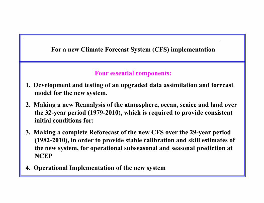
For a new Climate Forecast System (CFS) implementation

Four essential components:

1.  Development and testing of an upgraded data assimilation and forecast model for the new system.

2.  Making a new Reanalysis of the atmosphere, ocean, seaice and land over the 32-year period (1979-2010), which is required to provide consistent initial conditions for:

3.  Making a complete Reforecast of the new CFS over the 29-year period (1982-2010), in order to provide stable calibration and skill estimates of the new system, for operational subseasonal and seasonal prediction at NCEP

4.  Operational Implementation of the new system

The NCEP Climate Forecast System Reanalysis

Suranjana Saha, Shrinivas Moorthi, Hua-Lu Pan, Xingren Wu, Jiande Wang, Sudhir Nadiga, Patrick Tripp, Robert Kistler, John Woollen, David Behringer, Haixia Liu, Diane Stokes, Robert Grumbine, George Gayno, Jun Wang, Yu-Tai Hou, Hui-ya Chuang, Hann-Ming H. Juang, Joe Sela, Mark Iredell, Russ Treadon, Daryl Kleist, Paul Van Delst, Dennis Keyser, John Derber, Michael Ek, Jesse Meng, Helin Wei, Rongqian Yang, Stephen Lord, Huug van den Dool, Arun Kumar, Wanqiu Wang, Craig Long, Muthuvel Chelliah, Yan Xue, Boyin Huang, Jae-Kyung Schemm, Wesley Ebisuzaki, Roger Lin, Pingping Xie, Mingyue Chen, Shuntai Zhou, Wayne Higgins, Cheng-Zhi Zou, Quanhua Liu, Yong Chen, Yong Han, Lidia Cucurull, Richard W. Reynolds, Glenn Rutledge, Mitch Goldberg

Bulletin of the American Meteorological Society Volume 91, Issue 8, pp 1015-1057. doi: 10.1175/2010BAMS3001.1

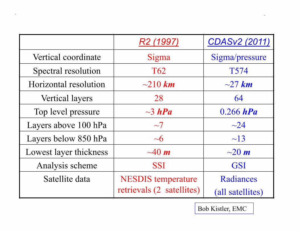
R2 (1997) CDASv2 (2011)

Vertical coordinate Sigma Sigma/pressure Spectral resolution T62 T574

Horizontal resolution ~210 km ~27 km Vertical layers 28 64

Top level pressure ~3 hPa 0.266 hPa Layers above 100 hPa ~7 ~24 Layers below 850 hPa ~6 ~13 Lowest layer thickness ~40 m ~20 m

Analysis scheme SSI GSI Satellite data NESDIS temperature

retrievals (2 satellites) Radiances

(all satellites)

Bob Kistler, EMC

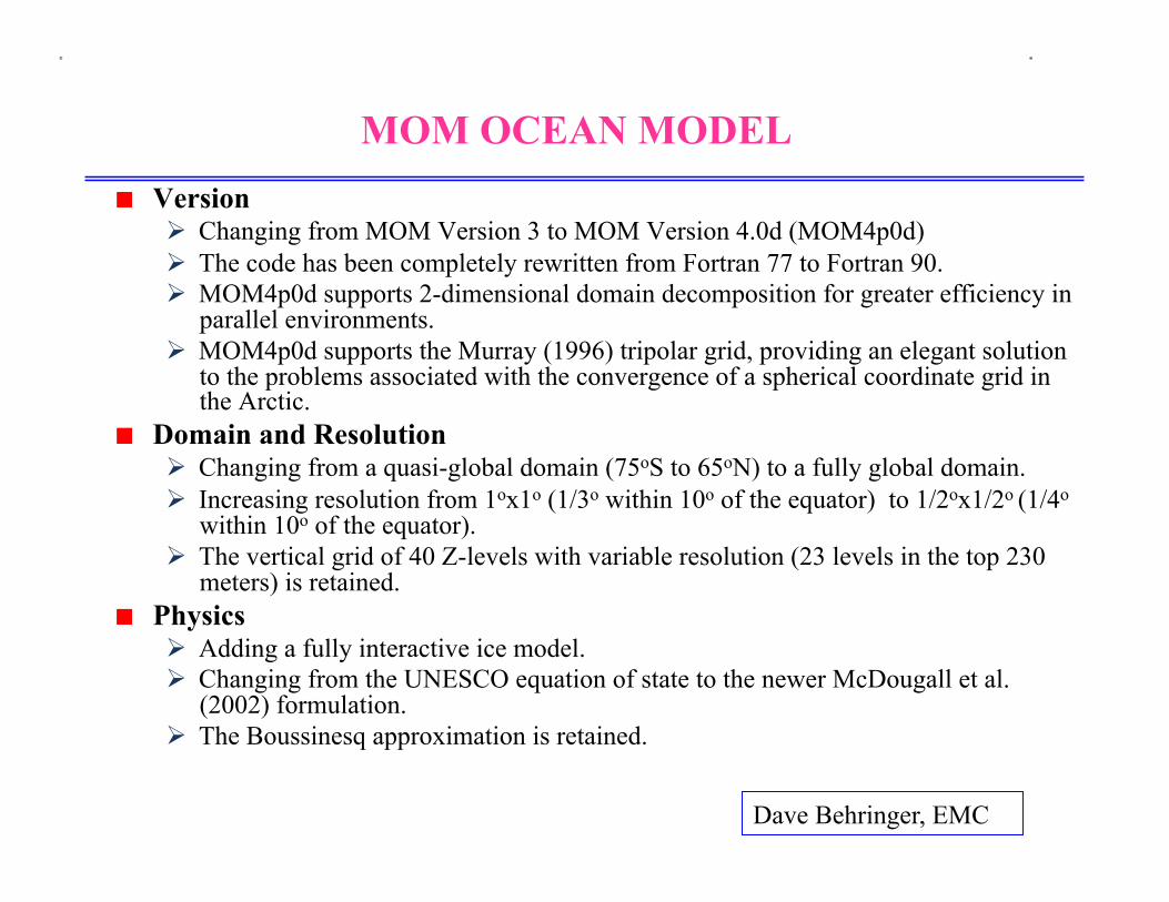
MOM OCEAN MODEL !   Version

  Changing from MOM Version 3 to MOM Version 4.0d (MOM4p0d)   The code has been completely rewritten from Fortran 77 to Fortran 90.   MOM4p0d supports 2-dimensional domain decomposition for greater efficiency in

parallel environments.   MOM4p0d supports the Murray (1996) tripolar grid, providing an elegant solution

to the problems associated with the convergence of a spherical coordinate grid in the Arctic.

!   Domain and Resolution   Changing from a quasi-global domain (75oS to 65oN) to a fully global domain.   Increasing resolution from 1ox1o (1/3o within 10o of the equator) to 1/2ox1/2o (1/4o

within 10o of the equator).   The vertical grid of 40 Z-levels with variable resolution (23 levels in the top 230

meters) is retained. !   Physics

  Adding a fully interactive ice model.   Changing from the UNESCO equation of state to the newer McDougall et al.

(2002) formulation.   The Boussinesq approximation is retained.

Dave Behringer, EMC

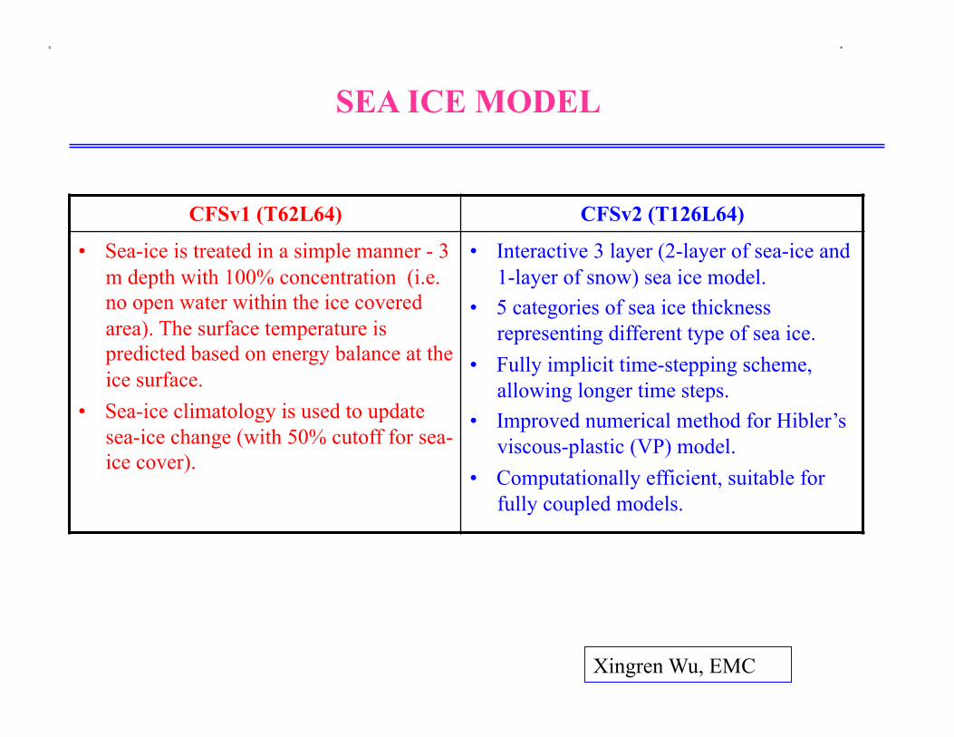
CFSv1 (T62L64) CFSv2 (T126L64)

•  Sea-ice is treated in a simple manner - 3 m depth with 100% concentration (i.e. no open water within the ice covered area). The surface temperature is predicted based on energy balance at the ice surface.

•  Sea-ice climatology is used to update sea-ice change (with 50% cutoff for sea-ice cover).

•  Interactive 3 layer (2-layer of sea-ice and 1-layer of snow) sea ice model.

•  5 categories of sea ice thickness representing different type of sea ice.

•  Fully implicit time-stepping scheme, allowing longer time steps.

•  Improved numerical method for Hibler’s viscous-plastic (VP) model.

•  Computationally efficient, suitable for fully coupled models.

SEA ICE MODEL

Xingren Wu, EMC

LAND SURFACE MODEL

CFSv1 (T62L64) •  2 soil layers (10, 190 cm) •  No frozen soil physics

•  Only one snowpack state (SWE) •  Surface fluxes not weighted by snow

fraction •  Vegetation fraction never less than 50% •  Spatially constant root depth •  Runoff & infiltration do not account for

subgrid variability of precipitation & soil moisture

•  Poor soil and snow thermal conductivity, especially for thin snowpack

CFSv2 (T126L64) •  4 soil layers (10, 30, 60, 100 cm) •  Frozen soil physics included •  Add glacial ice treatment •  Two snowpack states (SWE, density) •  Surface fluxes weighted by snow cover

fraction •  Improved seasonal cycle of vegetation •  Spatially varying root depth •  Runoff and infiltration account for sub-grid

variability in precipitation & soil moisture

•  Improved thermal conduction in soil/snow

•  Higher canopy resistance •  Improved evaporation treatment over bare soil

and snowpack

Mike Ek, EMC

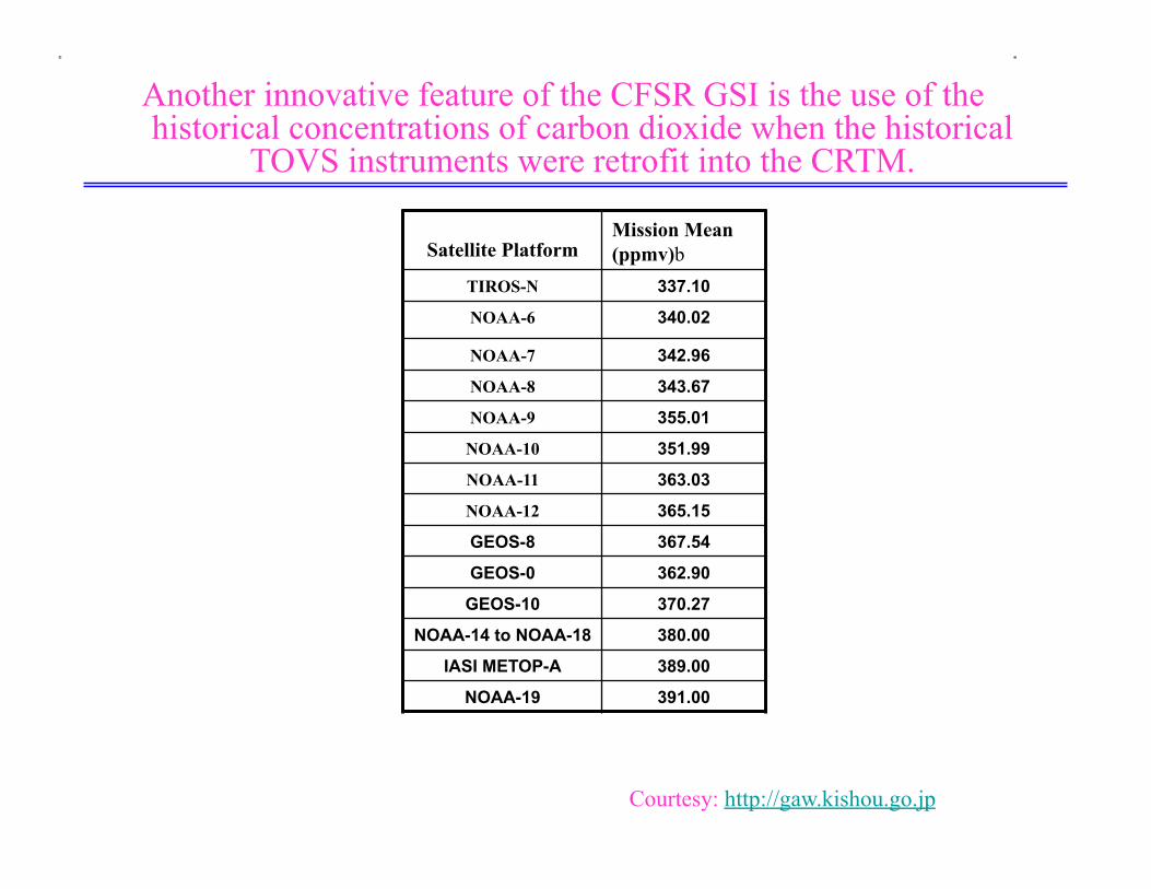
Another innovative feature of the CFSR GSI is the use of the historical concentrations of carbon dioxide when the historical

TOVS instruments were retrofit into the CRTM.

Satellite Platform Mission Mean (ppmv)b

TIROS-N 337.10

NOAA-6 340.02

NOAA-7 342.96

NOAA-8 343.67

NOAA-9 355.01

NOAA-10 351.99

NOAA-11 363.03

NOAA-12 365.15

GEOS-8 367.54

GEOS-0 362.90

GEOS-10 370.27

NOAA-14 to NOAA-18 380.00

IASI METOP-A 389.00

NOAA-19 391.00

Courtesy: http://gaw.kishou.go.jp

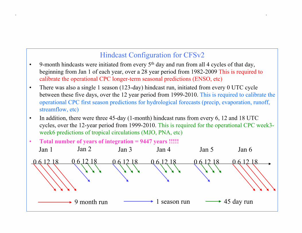
Hindcast Configuration for CFSv2 •  9-month hindcasts were initiated from every 5th day and run from all 4 cycles of that day,

beginning from Jan 1 of each year, over a 28 year period from 1982-2009 This is required to calibrate the operational CPC longer-term seasonal predictions (ENSO, etc)

•  There was also a single 1 season (123-day) hindcast run, initiated from every 0 UTC cycle between these five days, over the 12 year period from 1999-2010. This is required to calibrate the operational CPC first season predictions for hydrological forecasts (precip, evaporation, runoff, streamflow, etc)

•  In addition, there were three 45-day (1-month) hindcast runs from every 6, 12 and 18 UTC cycles, over the 12-year period from 1999-2010. This is required for the operational CPC week3-week6 predictions of tropical circulations (MJO, PNA, etc)

•  Total number of years of integration = 9447 years !!!!! Jan 1

0 6 12 18

9 month run 1 season run 45 day run

Jan 2

0 6 12 18

Jan 3

0 6 12 18

Jan 4

0 6 12 18

Jan 5

0 6 12 18

Jan 6

0 6 12 18

RESULTS

•  MJO INDEX

•  2-METER TEMPERATURE

•  PRECIPITATION

•  SST

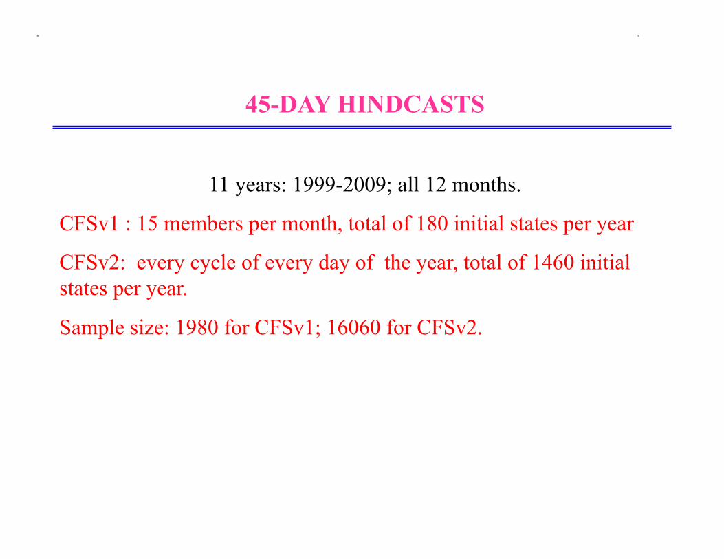
45-DAY HINDCASTS

11 years: 1999-2009; all 12 months.

CFSv1 : 15 members per month, total of 180 initial states per year

CFSv2: every cycle of every day of the year, total of 1460 initial states per year.

Sample size: 1980 for CFSv1; 16060 for CFSv2.

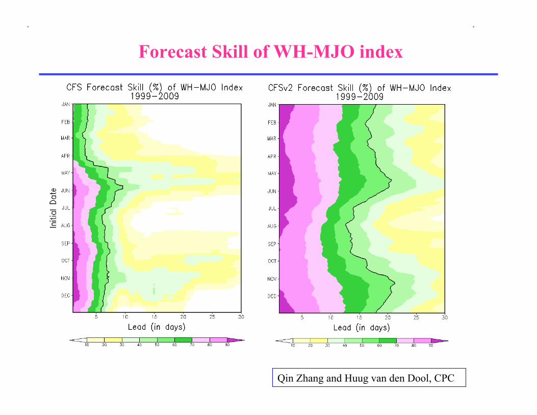
Forecast Skill of WH-MJO index

Qin Zhang and Huug van den Dool, CPC

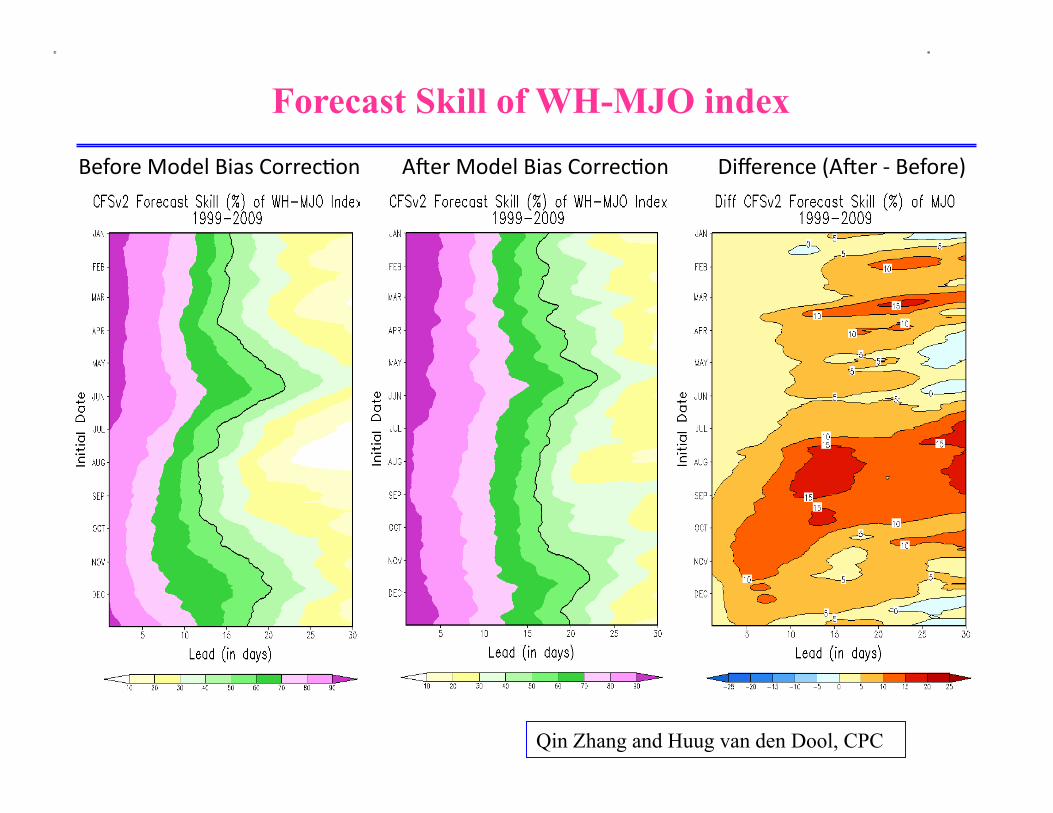
Before  Model  Bias  Correc/on   A2er  Model  Bias  Correc/on   Difference  (A2er  -­‐  Before)  

Qin Zhang and Huug van den Dool, CPC

Forecast Skill of WH-MJO index

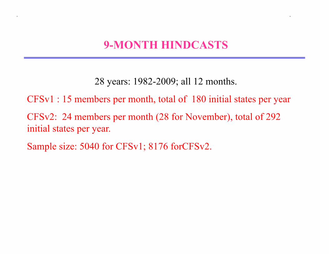
9-MONTH HINDCASTS

28 years: 1982-2009; all 12 months.

CFSv1 : 15 members per month, total of 180 initial states per year

CFSv2: 24 members per month (28 for November), total of 292 initial states per year.

Sample size: 5040 for CFSv1; 8176 forCFSv2.

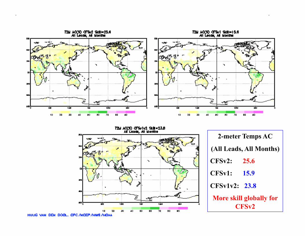
2-meter Temps AC

(All Leads, All Months)

CFSv2: 25.6

CFSv1: 15.9

CFSv1v2: 23.8

More skill globally for CFSv2

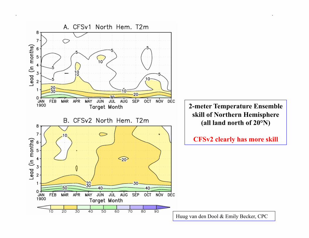
2-meter Temperature Ensemble skill of Northern Hemisphere

(all land north of 20°N)

CFSv2 clearly has more skill

Huug van den Dool & Emily Becker, CPC

Precipitation AC

(All Leads, All Months)

CFSv2: 14.9

CFSv1: 13.3

CFSv1v2: 16.2

More skill in the Western Pacific for

CFSv2

Sea Surface Temp AC

(All Leads, All Months)

CFSv2: 36.5

CFSv1: 32.4

CFSv1v2: 40.1

More skill west of the dateline and over the Atlantic for CFSv2

Huug van den Dool & Emily Becker, CPC

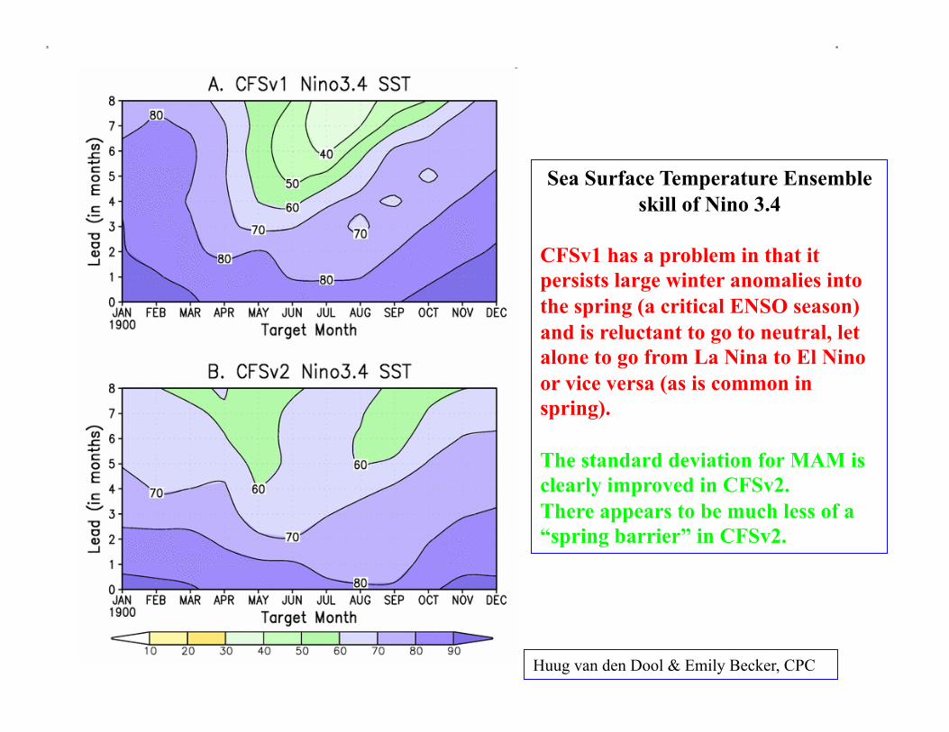
Sea Surface Temperature Ensemble skill of Nino 3.4

CFSv1 has a problem in that it persists large winter anomalies into the spring (a critical ENSO season) and is reluctant to go to neutral, let alone to go from La Nina to El Nino or vice versa (as is common in spring).

The standard deviation for MAM is clearly improved in CFSv2. There appears to be much less of a “spring barrier” in CFSv2.

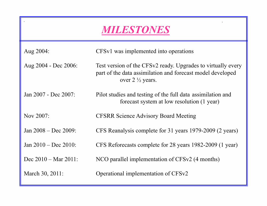
MILESTONES

Aug 2004: CFSv1 was implemented into operations

Aug 2004 - Dec 2006: Test version of the CFSv2 ready. Upgrades to virtually every part of the data assimilation and forecast model developed over 2 ½ years.

Jan 2007 - Dec 2007: Pilot studies and testing of the full data assimilation and forecast system at low resolution (1 year)

Nov 2007: CFSRR Science Advisory Board Meeting

Jan 2008 – Dec 2009: CFS Reanalysis complete for 31 years 1979-2009 (2 years)

Jan 2010 – Dec 2010: CFS Reforecasts complete for 28 years 1982-2009 (1 year)

Dec 2010 – Mar 2011: NCO parallel implementation of CFSv2 (4 months)

March 30, 2011: Operational implementation of CFSv2

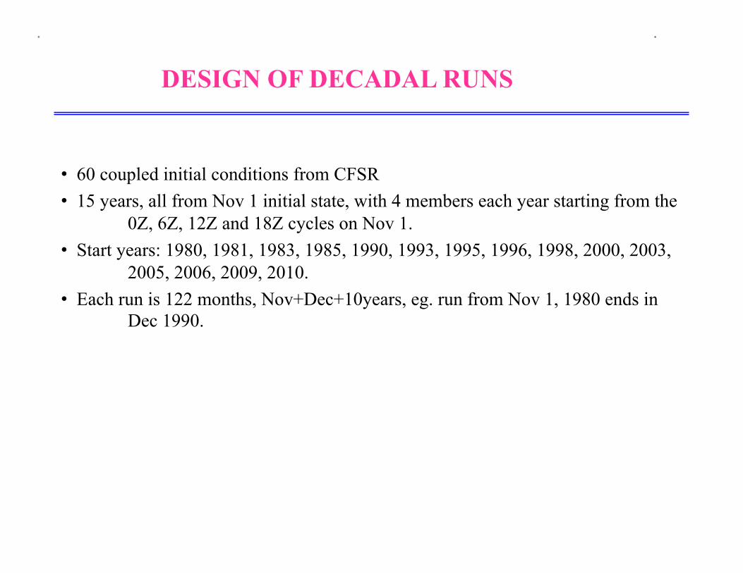
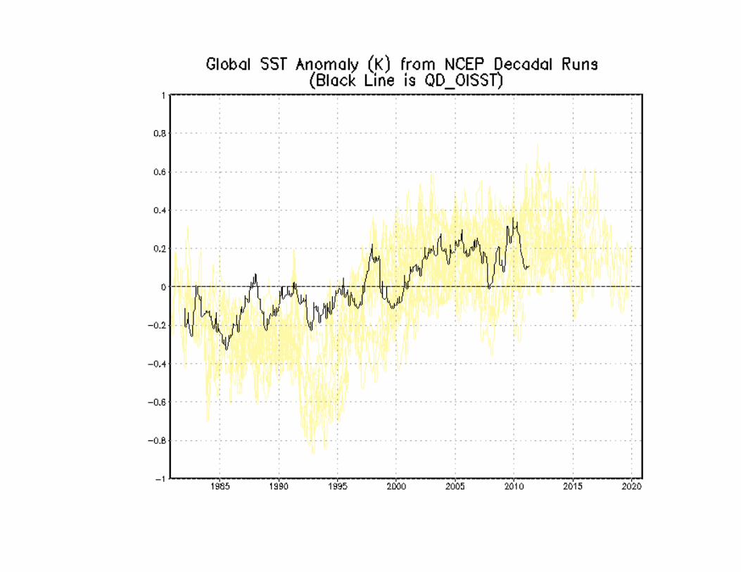
DESIGN OF DECADAL RUNS

•  60 coupled initial conditions from CFSR •  15 years, all from Nov 1 initial state, with 4 members each year starting from the

0Z, 6Z, 12Z and 18Z cycles on Nov 1. •  Start years: 1980, 1981, 1983, 1985, 1990, 1993, 1995, 1996, 1998, 2000, 2003,

2005, 2006, 2009, 2010. •  Each run is 122 months, Nov+Dec+10years, eg. run from Nov 1, 1980 ends in

Dec 1990.

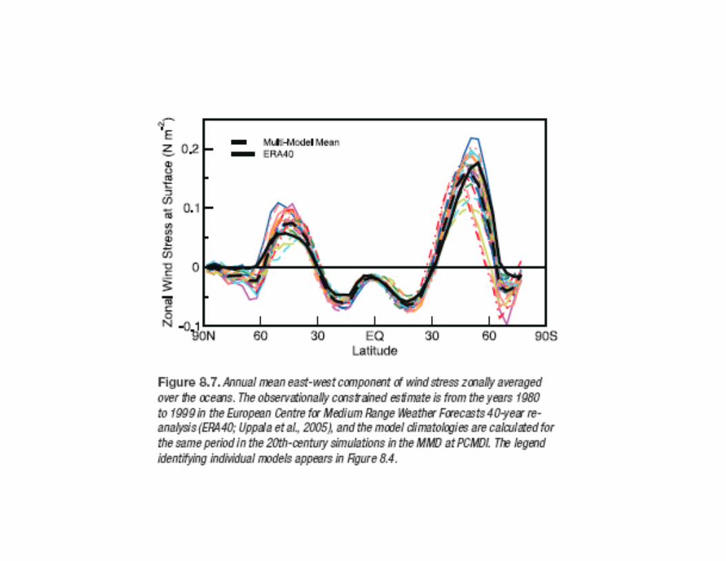
Annual mean zonal wind stress averaged over oceans

l model CFSR

TAU

X(W

/m-2

)

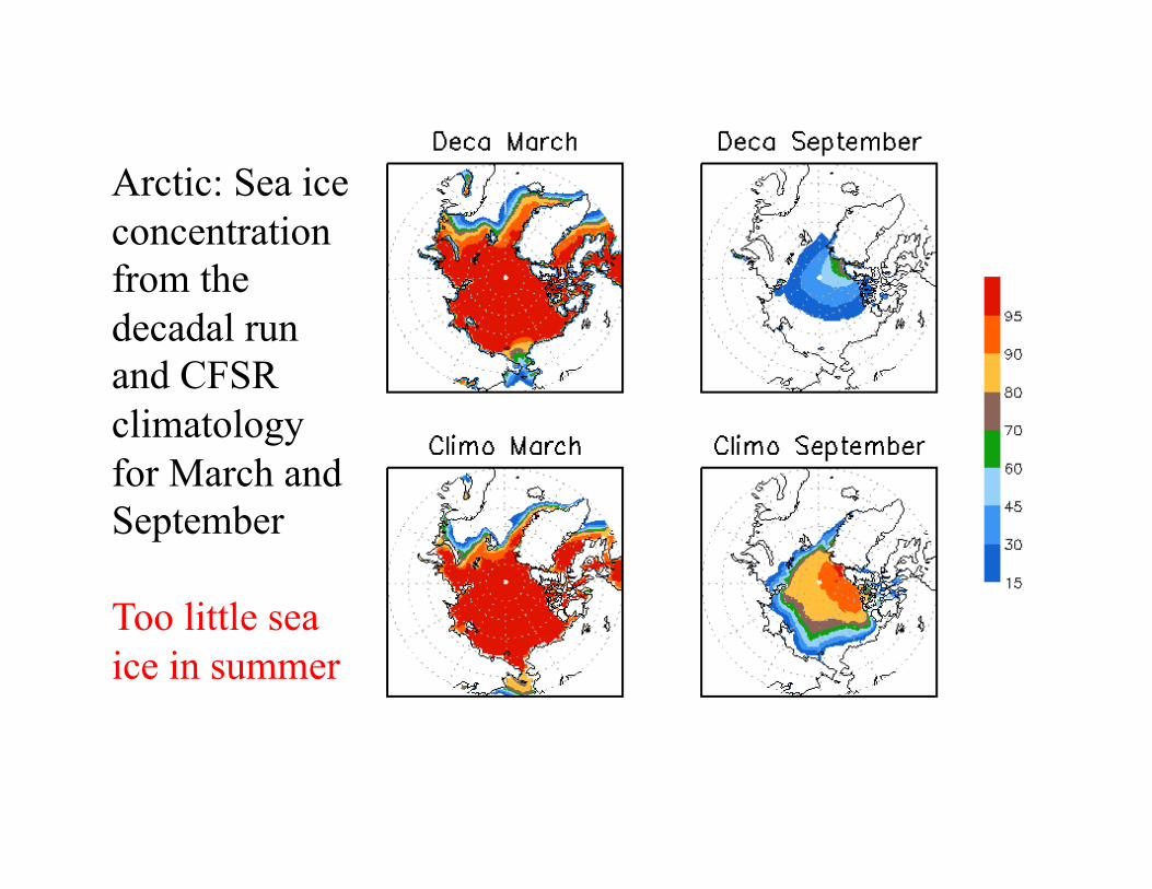
Arctic: Sea ice concentration from the decadal run and CFSR climatology for March and September

Too little sea ice in summer    

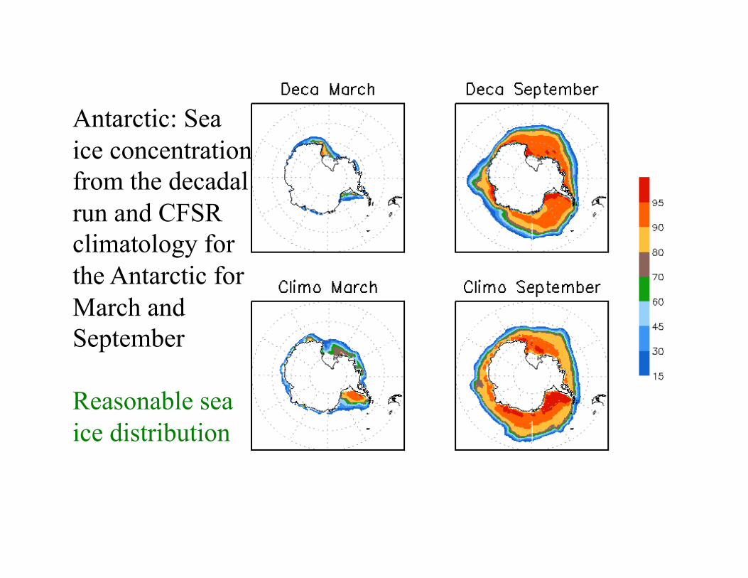
Antarctic: Sea ice concentration from the decadal run and CFSR climatology for the Antarctic for March and September

Reasonable sea ice distribution

SUMMARY OF SEA ICE ANALYSIS FROM DECADAL RUNS

•  Reasonable seasonal cycle for sea ice distribution is simulated for the ice coverage.

•  Ice is too thin in both polar regions. •  Ice is less extensive for the summer.

Future improvements •  Improve the sea ice thickness in the ICs by applying observational

data for assimilation. •  Improve the sea ice model by tuning parameters such as ice/snow

albedo.

0

0.05

0.1

0.15

0.2

0.25

0.3

0 0.25 0.5 0.75 1

Pow

er K

*K

Frequency (cycles per year)

Power Spectrum Nino34: CMIP'88; 43 years

0

0.05

0.1

0.15

0.2

0.25

0.3

0 0.25 0.5 0.75 1

Pow

er K

*K

Frequency (cycles per year)

Power Spectrum Nino34: CMIP'96; 52 years

0

0.05

0.1

0.15

0.2

0.25

0.3

0 0.25 0.5 0.75 1

Pow

er K

*K

Frequency (cycles per year)

Power Spectrum Nino34: OBS (62 years)

0

0.05

0.1

0.15

0.2

0.25

0.3

0 0.25 0.5 0.75 1

Pow

er K

*K

Frequency (cycles per year)

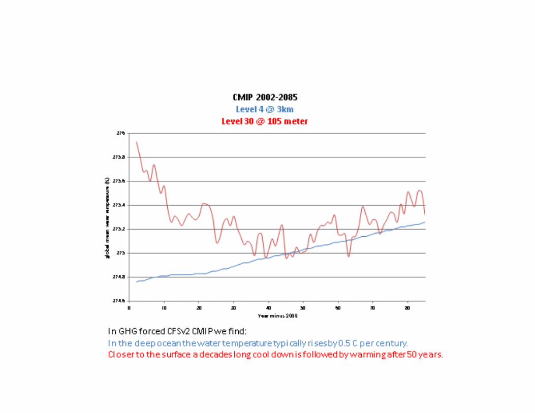
Power Spectrum Nino34: CMIP'02; 84 years

Different  CMIP  runs  and  OBS  have  somewhat  different    variance.  The  spectrum  is  noisy  but  generally  broadband  between  2  and  5  year  periods.    CFSv1  was  much  more  peaked.