Performance of Reclaimed Asphalt Pavement on Unpaved … · · 2013-05-22Performance of Reclaimed...

Performance of Reclaimed Asphalt Pavement on Unpaved Roads

Scott Koch

George Huntington, P.E. Khaled Ksaibati, PhD., P.E.

Wyoming Technology Transfer Center

University of Wyoming Laramie, Wyoming

May 2013

Acknowledgments

The authors would like to thank all the employees of Laramie, Johnson and Sweetwater counties who assisted with this project. Without their expertise, assistance, and cooperation, this study could not have been conducted. Thanks to the Desert Mountain Corporation for their expertise and assistance on the Sweetwater County sections. We would also like to thank the Wyoming Department of Transportation for their support of this project. Finally, we would like to thank Mary Harman, Bart Evans, Josh Jones, Burt Andreen, Jonathan Zumwalt, and Harry Rocheville for their work on this project.

Disclaimer

The contents of this report reflect the work of the authors, who are responsible for the facts and the accuracy of the information presented. Mention of specific products is for informational purposes only and does not constitute any endorsement. This document does not constitute any policy of or endorsement by the Mountain-Plains Consortium or the University of Wyoming.This document is disseminated under the sponsorship of the Mountain-Plains Consortium in the interest of information exchange. The U.S. Government assumes no liability for the contents or use thereof.

North Dakota State University does not discriminate on the basis of age, color, disability, gender expression/identity, genetic information, marital status, national origin, public assistance status, sex, sexual orientation, status as a U.S. veteran., race or religion. Direct inquiries to the Vice President for Equity, Diversity and Global Outreach, 205 Old Main, (701) 231-7708.

TABLE OF CONTENTS

1. Introduction ........................................................................................................................... 1

1.1 Background ...................................................................................................................... 1

1.2 Problem Statement ........................................................................................................... 1

1.3 Research Objectives ......................................................................................................... 2

1.4 Report Organization ......................................................................................................... 3

2. Literature Review ................................................................................................................. 5

2.1 Asphalt Pavement Reclamation and Recycling ............................................................... 5

2.2 Obtaining Reclaimed Asphalt Pavement.......................................................................... 6

2.3 Uses of Reclaimed Asphalt Pavement ............................................................................. 6

2.3.1 In-Place Recycling .................................................................................................... 7

2.3.2 Hot Mix Asphalt and Reclaimed Asphalt Pavement (RAP) ..................................... 8

2.3.3 Cold Mix Asphalt (Central Processing Facility) ....................................................... 8

2.3.4 Full Depth Reclamation ............................................................................................ 8

2.3.5 Embankment or Fill .................................................................................................. 8

2.3.6 Mechanically Stabilized Earth Walls ........................................................................ 9

2.4 Economics of Reclaimed Asphalt Pavement (RAP) ........................................................ 9

2.4.1 RAP in Hot Mix Asphalt........................................................................................... 9

2.4.2 RAP in Road Base .................................................................................................. 12

2.5 Unpaved Roads .............................................................................................................. 12

2.5.1 Gravel Road Distresses ........................................................................................... 13

2.5.2 Dust Control ............................................................................................................ 16

2.5.3 Dust Collection and Measurement .......................................................................... 19

2.6 Literature Review Summary .......................................................................................... 20

3. Methodology ........................................................................................................................ 21

3.1 Test Section Descriptions ............................................................................................... 21

3.1.1 Site Layouts ............................................................................................................ 23

3.1.2 Traffic ..................................................................................................................... 25

3.1.3 Surfacing Materials: Aggregate, RAP and Cement-Treated Base (CTB) ............. 25

3.1.4 Dust Suppression Agents ........................................................................................ 33

3.2 Testing Methods ............................................................................................................. 34

3.2.1 Aggregate ................................................................................................................ 34

3.2.2 Weather ................................................................................................................... 34

3.2.3 Dust Assessment ..................................................................................................... 34

3.2.4 Roadway Condition Evaluations: URCI ................................................................ 37

3.3 Construction Methods .................................................................................................... 37

3.3.1 Laramie County: Blade Mixed............................................................................... 37

3.3.2 Johnson County: Stockpile Mixed ......................................................................... 40

3.3.3 Sweetwater County: Reclaimer Mixed .................................................................. 45

3.4 Summary of Methodologies ........................................................................................... 52

4. Results .................................................................................................................................. 53

4.1 Visual Dust Ratings vs Dustometer Measurements ....................................................... 53

4.2 Environmental Effects on Dust Measurements .............................................................. 56

4.2.1 Dust vs Age ............................................................................................................. 56

4.2.2 Dust vs Moisture Content ....................................................................................... 57

4.2.3 Dust vs Wind Speed ................................................................................................ 57

4.3 Laramie County .............................................................................................................. 60

4.3.1 Materials Properties ................................................................................................ 60

4.3.2 Visual Observations ................................................................................................ 64

4.3.3 Unsurfaced Road Condition Index (URCI) ............................................................ 68

4.3.4 Dust Emissions........................................................................................................ 69

4.4 Johnson County .............................................................................................................. 72



4.4.3 Unsurfaced Road Condition Index.......................................................................... 77

4.4.4 Dust Emissions........................................................................................................ 77

4.5 Sweetwater County ........................................................................................................ 78



4.5.3 Unsurfaced Road Condition Index.......................................................................... 94

4.5.4 Dust Emissions........................................................................................................ 98

4.6 Summary of Results ..................................................................................................... 100

5. Economic Analyses............................................................................................................ 103

5.1 Study Section: Sweetwater County Road 23: Crooks Gap Road ................................ 103

5.2 Cost-Benefit Analysis Method ..................................................................................... 103

5.3 Data Collection ............................................................................................................. 103

5.4 Cost Evaluations ........................................................................................................... 104

5.4.1 RAP in Hot Plant Mix (RHPM) ............................................................................ 104

5.4.2 RAP in Road Base ................................................................................................ 104

5.4.3 RAP in Gravel Roads ............................................................................................ 105

5.5 Data Analysis ............................................................................................................... 105

5.5.1 Step A: Dust Reduction ....................................................................................... 105

5.5.2 Step B: Layer Coefficients ................................................................................... 106

5.5.3 Step C: Haul Costs ............................................................................................... 106

5.5.4 Step D: Savings from Virgin Aggregate .............................................................. 106

5.5.5 Step E: Total Benefit ............................................................................................ 106

5.6 Case Study .................................................................................................................... 107

5.6.1 RAP in Hot Plant Mix (RHPM) ............................................................................ 107

5.6.2 Road Base with RAP ............................................................................................ 109

5.6.3 RAP in Gravel Roads ............................................................................................ 110

5.7 Summary of Economic Analysis of RAP Use ............................................................. 110

6. Summary and Conclusions .............................................................................................. 113

6.1 Laramie County Performance Summary ...................................................................... 113

6.2 Johnson County Performance Summary ...................................................................... 113

6.3 Sweetwater County Performance Summary ................................................................ 113

6.4 Performance as a Function of Construction Methods .................................................. 114

6.5 Performance as a Function of Surfacing Materials ...................................................... 115

6.6 Performance as a Function of Dust Suppressants ........................................................ 115

6.7 Economics of RAP Use ................................................................................................ 116

6.8 Dust Measurements with the CSU Dustometer............................................................ 117

7. Recommendations ............................................................................................................. 119

8. References .......................................................................................................................... 121

Appendix A. Dust, Moisture and Wind Data ........................................................................ 125

A.1 Laramie County Dustometer, Moisture and Wind Data ................................................. 125

A.2 Johnson County Dustometer, Moisture and Wind Data ................................................. 128

A.3 Laramie County Moisture Content Summary ................................................................. 130

A.4 Johnson County Moisture Content Summary ................................................................. 133

A.5 Sweetwater County Moisture Content Summary............................................................ 135

A.6 Laramie County Dustometer Measurement Summary .................................................... 136

A.7 Johnson County Dustometer Measurement Summary .................................................... 139

A.8 Sweetwater County Dustometer Measurement and Visual Dust Rating Summary ........ 141

Appendix B. Unsurfaced Road Condition Indexes ............................................................... 143

B.1 Laramie County URCI and Deduct Values ..................................................................... 143

B.2 Johnson County URCI and Deduct Values ..................................................................... 145

B.3 Sweetwater County URCI and Deduct Values ............................................................... 146

Appendix C. Gradations .......................................................................................................... 147

C.1 Laramie County Gradations (% Passing) ........................................................................ 147

C.2 Johnson County Gradations (% Passing) ........................................................................ 148

C.3 Sweetwater County Gradations (% Passing) ................................................................... 149

Appendix D. Traffic and Other Data ..................................................................................... 151

D.1 Johnson and Laramie County General Section Data ...................................................... 151

D.2 Johnson County Traffic Data .......................................................................................... 151

Appendix E. Abbreviations ..................................................................................................... 153

LIST OF TABLES

Table 2.1 Materials Cost Comparison: Virgin HMA vs RAP-Virgin HMA (Kandhal 1997) ....................................................................................................... 11

Table 2.2 HMA Cost Savings at Various RAP Contents (Kandhal 1997) ............................. 11

Table 2.3 Asphalt Recycling Cost Savings by Region in 1984 (Kandhal 1997) ................... 11

Table 3.1 Laramie County Test Sections ............................................................................... 25

Table 3.2 Johnson County Test Sections ................................................................................ 25

Table 3.3 Sweetwater County Test Sections .......................................................................... 30

Table 3.4 Approximate Test Section Traffic Volumes and Speeds ....................................... 30

Table 4.1 Suggested Numerical Cutoffs for Data Generated with the Dustometer to Relate Measured Dust to Subjective Dust Severity Ratings. ................................. 55

Table 4.2 Laramie County RAP Materials Test Results ........................................................ 61

Table 4.3 Laramie County Virgin Aggregate Materials Test Results .................................... 62

Table 4.4 Laramie County Surface Blended Materials Test Results ...................................... 63

Table 4.5 Laramie County As-Built Interpolated RAP Contents ........................................... 64

Table 4.6 Johnson County Stockpiled Virgin Aggregate Materials Properties ...................... 72

Table 4.7 Johnson County Surfacing Blend Materials Properties .......................................... 73

Table 5.1 WYDOT 2010 Weighted Average Bid Prices for Hot Plant Mix Asphalt .......... 104

Table 5.2 WYDOT Materials and Rates Summary for RAP in Hot Plant Mix (RHPM) .... 104

Table 5.3 WYDOT Materials and Rates Summary for Road Base With and Without RAP ...................................................................................................................... 105

Table 5.4 Benefit Analysis Template Using All Factors ...................................................... 107

Table 5.5 RHPM Material Calculations ............................................................................... 108

Table 5.6 Cost Saving by Using RHPM Instead of HPM .................................................... 108

Table 5.7 Cost Savings from Using RHPM Instead of HPM ............................................... 109

Table 5.8 Cost of Road Base With and Without RAP ......................................................... 109

Table 5.9 Cost-Benefit Analysis for RAP in Road Base ...................................................... 109

Table 5.10 Cost-Benefit Analysis for RAP in Gravel Roads ................................................. 110

LIST OF FIGURES

Figure 1.1 USEPA non-attainment areas for PM-10 particulate matter, December 2010 (USEPA 2011) .......................................................................................................... 2

Figure 3.1 Laramie County test sites ....................................................................................... 21

Figure 3.2 Johnson County test site ......................................................................................... 22

Figure 3.3 Sweetwater County test site ................................................................................... 22

Figure 3.4 Wyoming test site locations ................................................................................... 23

Figure 3.5 Laramie County Atlas Road test sections. .............................................................. 24

Figure 3.6 Laramie County Pry Road test sections. ................................................................ 24

Figure 3.7 Johnson County test sections on Schoonover Road, JO CR 204B. ........................ 26

Figure 3.8 Sweetwater County test segments on Crooks Gap Road, SW CR 23, south end. .. 27

Figure 3.9 Sweetwater County test segments on Crooks Gap Road, SW CR 23, center. ....... 28

Figure 3.10 Sweetwater County test segments on Crooks Gap Road, SW CR 23, north end. .. 29

Figure 3.11 Laramie County material source locations. ............................................................ 31

Figure 3.12 Blending of aggregate at Laramie County scoria pit near Atlas Road. .................. 32

Figure 3.13 Crooks Gap Road north of the test sections showing the surfacing material typical of that which was blended with RAP or CTB on the Sweetwater County test sections. ............................................................................................................ 33

Figure 3.14 CSU dustometer with open filter box. .................................................................... 35

Figure 3.15 Dustometer setup with, left to right, the dustometer, generator and vacuum. ........ 36

Figure 3.16 Scarifying Laramie County’s Atlas Road prior to placement and blending of RAP. ................................................................................................................... 38

Figure 3.17 Placement of RAP windrow on Laramie County’s Atlas Road with bottom- discharge haul trucks. ............................................................................................. 38

Figure 3.18 Blending RAP and existing, scarified aggregate on Laramie County’s Atlas Road. ....................................................................................................................... 39

Figure 3.19 Blending and shaping RAP and existing, scarified aggregate on Laramie County’s Atlas Road. ............................................................................................. 39

Figure 3.20 RAP and virgin aggregate stockpiles at Johnson County’s Piney Creek stockpiles, June 2008. ............................................................................................. 40

Figure 3.21 Initial shaping of Johnson County’s Schoonover Road prior to placement of the blended RAP and aggregate, June 2008. ................................................................ 41

Figure 3.22 Placing RAP and aggregate blend on Johnson County’s Schoonover Road, June 2008. ............................................................................................................... 41

Figure 3.23 Shaping RAP and aggregate blend on Johnson County’s Schoonover Road, June 2008. ............................................................................................................... 42

Figure 3.24 Compacting RAP and aggregate blend on Johnson County's Schoonover Road with pneumatic tire compactors mounted on the motor grader’s ripper hydraulics, June 2008. ............................................................................................................... 42

Figure 3.25 Final compaction of the RAP aggregate blend on Johnson County’s Schoonover Road, June 2008. .................................................................................................... 43

Figure 3.26 Calcium chloride flakes placed on damp RAP and aggregate blend on Johnson County’s Schoonover Road, June 2008. ................................................................ 43

Figure 3.27 Close-up of calcium chloride flakes on Johnson County’s Schoonover Road, June 2008. ............................................................................................................... 44

Figure 3.28 Calcium chloride flakes partially worked into the aggregate surface by traffic on Johnson County’s Schoonover Road, June 2008. .................................................. 44

Figure 3.29 Calcium chloride flakes mostly worked into the aggregate surface by traffic on Johnson County’s Schoonover Road, June 2008. .................................................. 45

Figure 3.30 Operation of the reclaimer used to blend the underlying, existing surface with RAP or CTB on Sweetwater County’s Crooks Gap Road. (1) Adjustable rear door. (2) Universal rotor. (3) Breaker bars. (4) Adjustable front door. ............... 46

Figure 3.31 Applying water to the CTB and aggregate blend prior to final shaping and compaction on Sweetwater County’s Crooks Gap Road, August 2010. ................ 46

Figure 3.32 Blending and shaping the existing aggregate and CTB blend on Sweetwater County’s Crooks Gap Road, August 2010. ............................................................ 47

Figure 3.33 Final shaping and compaction of CTB and aggregate blend using a motor grader with pneumatic tire compactors mounted to its ripper hydraulics on Sweetwater County’s Crooks Gap Road, August 2010. ............................................................ 47

Figure 3.34 Pre-wetting RAP and aggregate blend at dawn prior to application of dust suppressants on Sweetwater County’s Crooks Gap Road, July 2011. ................... 48

Figure 3.35 Dampened aggregate and RAP blend prepared for application of magnesium chloride and polymer dust suppressant on Sweetwater County’s Crooks Gap Road, July 2011. ..................................................................................................... 49

Figure 3.36 Shaping dampened RAP and aggregate blend in preparation for placement of dust suppressants on Sweetwater County’s Crooks Gap Road, July 2011. ........... 49

Figure 3.37 Applying dust suppressant brine to aggregate and RAP blend on Sweetwater County’s Crooks Gap Road, July 2011. ................................................................. 50

Figure 3.38 Recently applied magnesium chloride on the RAP and aggregate blend on Sweetater County’s Crooks Gap Road, July 2011. ................................................ 50

Figure 3.39 Magnesium chloride almost completely absorbed into the RAP and aggregate blend on Sweetwater County’s Crooks Gap Road, July 2011. .............................. 51

Figure 3.40 Compaction of the magnesium chloride-treated RAP and aggregate blend on Sweetwater County’s Crooks Gap Road, July 2011. ............................................. 51

Figure 4.1 Dust measured with the dustometer as a function of subjective visual dust ratings, with a suggested numerical cutoff between Medium and High dust severity at 1.00 grams per mile. ............................................................................................... 54

Figure 4.2 Dust measured with the dustometer as a function of subjective visual dust ratings, with suggested numerical cutoffs between High, Medium, Low and None dust severity. .................................................................................................................. 55

Figure 4.3 Measured dust as a function of road surface age on Johnson County’s Schoonover Road. ....................................................................................................................... 56

Figure 4.4 Measured dust as a function of road surface age on Laramie County’s Atlas and Pry Roads. .............................................................................................................. 57

Figure 4.5 Measured dust as a function of moisture content on Johnson County’s Schoonover Road, section S2 with RAP/aggregate blend and no calcium chloride. ................. 58

Figure 4.6 Measured dust as a function of moisture content on Laramie County’s Atlas Road, section A1 with blended RAP and existing aggregate. ................................ 58

Figure 4.7 Measured dust as a function of wind speed on Johnson County’s Schoonover Road, section S2 with RAP and aggregate surfacing but no calcium chloride. ..... 59

Figure 4.8 Measured dust as a function of wind speed on Laramie County’s Pry Road, section S1 with blended RAP and existing aggregate. ........................................... 59

Figure 4.9 Laramie County RAP average gradation of the milled material. ........................... 60

Figure 4.10 Segregation of RAP on Laramie County’s Atlas Road in June 2008, two months after initial RAP application. .............................................................. 65

Figure 4.11 Segregation bands attributed to inadequate spreading of the windrows placed by the bottom-discharge haul trucks on Laramie County’s Pry Road in November 2008, six months after initial application. ............................................ 65

Figure 4.12 Nearly 100% RAP resulting in excessive loose aggregate on Laramie County’s Atlas Road in June 2008, about two months after initial application. .................... 66

Figure 4.13 Well compacted, tight surface due to good blending on Laramie County’s Atlas Road in June 2008, about two months afetr initial application. .................... 66

Figure 4.14 Re-working Laramie County’s Pry Road in August 2008, four months after initial application, to correct segregation with additional blending and spreading. 67

Figure 4.15 Good, tight surface on Laramie County’s Atlas Road in October 2008, five months after initial application and two months after re-blending with motor grader. ..................................................................................................................... 68

Figure 4.16 Variable densification under traffic due to incomplete blending and segregation of RAP and aggregate on Laramie County’s Pry Road in November 2008, six months after initial compaction and three months after re-working. .................................. 69

Figure 4.17 Aggregate only forming a good driving surface on Laramie County’s Pry Road in July 2008, two months after shaping. ................................................................. 70

Figure 4.18 Aggregate only forming a good driving surface on Laramie County’s Atlas Road in September 2008, four months after shaping. ............................................ 70

Figure 4.19 Laramie County unsurfaced road condition indexes (URCI) and deduct values for potholes, ruts and loose aggregate (LA). .......................................................... 71

Figure 4.20 Dust measured with the dustometer on the Laramie County RAP blend and aggregate only (G) test segments. .......................................................................... 71

Figure 4.21 Road surface with some rutting on Johnson County’s Schoonover Road, segment S1 with RAP and calcium chloride in August 2008, two months after RAP placement and one month after calcium chloride application. .............. 74

Figure 4.22 Road surface on Johnson County’s Schoonover Road, segment S2 with RAP blend but no calcium chloride in August 2008, two months after RAP placement. ...................................................................................................... 75

Figure 4.23 Road surface on Johnson County’s Schoonover Road, segment S0 with aggregate and calcium chloride in September 2008, two months after calcium chloride application. ................................................................................. 75

Figure 4.24 Road surface on Johnson County’s Schoonover Road, segment S1 with RAP and calcium chloride in October 2008, four months after RAP placement and three months after calcium chloride application. ................................................... 76

Figure 4.25 Road surface on Johnson County’s Schoonover Road, segment S2 with RAP but no calcium chloride in October 2008, four months after RAP placement. ...... 76

Figure 4.26 Unsurfaced road condition indexes and deduct values for ruts and loose aggregate (LA) on Johnson County’s Schoonover Road for segments S0 with gravel and calcium chloride (G&C), S1 with RAP blend and calcium chloride, and S2 with RAP blend only. ..................................................................................................... 77

Figure 4.27 Dust measurements from the dustometer before and after calcium chloride application on Johnson County’s Schoonover Road for segments S0 with gravel and calcium chloride, S1 with RAP blend and calcium chloride, and S2 with RAP blend only. ..................................................................................................... 78

Figure 4.28 Average gradations of in-place crushed base (CB), milled cement-treated base (CTB) blend, and reclaimed asphalt pavement (RAP) blend from Sweetwater County’s Crooks Gap Road, October 2010, two months after construction. ......... 79

Figure 4.29 Crushed base gradations within WYDOT Grading W specifications as collected from the roadway on section D of Sweetwater County’s Crooks Gap Road, October 2010, two months after construction. ....................................................... 79

Figure 4.30 Cement-treated base (CTB) and existing surfacing blended gradations with the average, minimum and maximum of 9 samples collected from sections E through J of the roadway on Sweetwater County’s Crooks Gap Road, October 2010, two months after construction. ............................................................................... 80

Figure 4.31 Reclaimed asphalt pavement (RAP) and existing surface blended gradations with the average, minimum and maximum of 6 samples collected from sections L through M on Sweetwater County’s Crooks Gap Road, October 2010, two months after construction. ...................................................................................... 80

Figure 4.32 Road surface made of limestone crushed base treated with magnesium chloride on Sweetwater County’s Crooks Gap Road. .......................................................... 81

Figure 4.33 Road surface made of limestone crushed base treated with magnesium chloride on Sweetwater County’s Crooks Gap Road showing small scale roughness. ........ 82

Figure 4.34 Dust from limestone crushed base before dust suppressant application on uphill, curved segment D of Sweetwater County’s Crooks Gap Road in June 2011. ....... 83

Figure 4.35 Dust from limestone crushed base before dust suppressant application on level, curved segement C on Sweetwater County’s Crooks Gap Road in June 2011. ..... 83

Figure 4.36 Crust formed by application of lignin and magnesium chloride dust suppressant applied to limestone crushed base on segment C of Sweetwater County’s Crooks Gap Road in August 2011, three weeks after application of dust suppressant. ..... 84

Figure 4.37 Road surface of limestone crushed base treated with lignin and magnesium chloride on uphill, curved segment D of Sweetwater County’s Crooks Gap Road in August 2011, three weeks after application of dust suppressant. ............. 84

Figure 4.38 Broken up crust of limestone crushed base, foreground, and still intact crust, background, both treated with lignin and magnesium chloride on uphill, curved segment D of Sweetwater County’s Crooks Gap Road in September 2011, eight weeks after application of dust suppressant. .......................................................... 85

Figure 4.39 Dust from road surfaced with finer reclaimed cement-treated base on segment G of Sweetwater County’s Crooks Gap Road in June 2011 before application of dust supressant. .................................................................................................. 86

Figure 4.40 Dust from road surfaced with coarser reclaimed cement-treated base on segment E of Sweetwater County’s Crooks Gap Road in June 2011 before application of dust suppressants. ............................................................................................... 87

Figure 4.41 Road surface with good crust made of reclaimed cement-treated base treated with magnesium chloride on segment F of Sweetwater County’s Crooks Gap Road in August 2011, three weeks after application of dust suppressant. ........................... 87

Figure 4.42 Road surface with good crust made of reclaimed cement-treated base treated with polymer and magnesium chloride on segement G of Sweetwater County’s Crooks Gap Road in August 2011, three weeks after application of dust suppessant. ....... 88

Figure 4.43 Dust from road surface made of reclaimed cement-treated base blended with existing aggregate and treated with magnesium chloride on segment J of Sweetwater County’s Crooks Gap Road in September 2011, eight weeks after application of dust suppressants. ............................................................................ 88

Figure 4.44 Road surface made from RAP blended with existing aggregate on segment M of Sweetwater County’s Crooks Gap Road in March 2011, before the application of dust suppressants. ................................................................................................... 89

Figure 4.45 Road surface made from RAP blended with existing aggregate on segment K of Sweetwater County’s Crooks Gap Road in April 2011, before application of dust suppressant. ............................................................................................................ 89

Figure 4.46 Road surface made from RAP blended with existing aggregate on segment Q of Sweetwater County’s Crooks Gap Road in April 2011 without dust suppression agents. ..................................................................................................................... 90

Figure 4.47 Road surface made from RAP blended with existing aggregate treated with magnesium chloride and polymer on segment M of Sweetwater County’s Crooks Gap Road in August 2011, three weeks after application of dust suppressant ............................................................................................................. 91

Figure 4.48 Road surface made from RAP blended with existing aggregate and treated with magnesium chloride on segment of Sweetwater County’s Crooks Gap Road in August 2011, three weeks after application of dust suppressant. ........................... 91

Figure 4.49 Road surface made from RAP blended with existing aggregate on segment P of Sweetwater County’s Crooks Gap Road in August 2011. ..................................... 92

Figure 4.50 Road surface made with RAP blended with existing aggregate and treated with magnesium chloride on segment N of Sweetwater County’s Crooks Gap Road in September 2011, eight weeks after application of dust suppressant. ..................... 92

Figure 4.51 Road surface made with RAP blended with existing aggregate and treated with magnesium chloride and polymer on segment L of Sweetwater County’s Crooks Gap Road in September 2011, eight weeks after application of dust suppressant. 93

Figure 4.52 Road surface made with RAP blended with existing aggregate on segment P of Sweetwater County’s Crooks Gap Road in September 2011. ................................ 93

Figure 4.53 Average unsurfaced road condition indexes (URCI) for test segments on Sweetwater County’s Crooks Gap Road in 2011. .................................................. 94

Figure 4.54 Average loose aggregate deduct values for test segments on Sweetwater County’s Crooks Gap Road in 2011. ...................................................................... 95

Figure 4.55 Average washboards/corrugations deduct values for test segments on Sweetwater County’s Crooks Gap Road in 2011. .................................................. 96

Figure 4.56 Average ruts deduct values for test segments on Sweetwater County’s Crooks Gap Road in 2011. .................................................................................................. 97

Figure 4.57 Average potholes deduct values for test segments on Sweetwater County’s Crooks Gap Road in 2011. ..................................................................................... 98

Figure 4.58 Average dust measured with the dustometer on test segments on Sweetwater County’s Crooks Gap Road in 2011, full scale. ..................................................... 99

Figure 4.59 Average dust measured with the dustometer on test segments on Sweetwater County’s Crooks Gap Road in 2011, partial scale. .............................................. 100

1

1. INTRODUCTION

1.1 Background

With the influx of oil and gas drilling in the Rocky Mountain region, local road networks are seeing substantial increases in traffic, particularly trucks. This often results in increased maintenance costs that are too costly for many local jurisdictions’ budgets.

Gravel loss, primarily in the form of dust, is a common problem on Wyoming’s gravel roads. This loss both degrades the road surface and creates environmental problems. For both engineering and environmental reasons, it is in the best interests of the roads’ owners and users to minimize dust loss and provide good road surfaces. As vehicles kick up dust, it blows away, and the unpaved surface loses the binding effects of fine particles. Then, surface distresses such as washboards—rhythmic corrugations—develop on the road surface. With the loss of fines, the surfacing material becomes more permeable, trapping more water on the surface, leading to more surface distresses such as potholes and ruts.

As dust enters the air, it increases the risk of violating federal air quality standards. Dust is considered a “particulate matter” made up of particles that are 10 micrometers (microns) or less, referred to as “PM-10.” Figure 1.1 shows the national distribution of non-attainment areas for PM-10 (USEPA 2011). Sheridan County, Wyoming, is one of these non-attainment areas. As more users travel Wyoming’s unpaved roads, the risk posed by fugitive dust will only increase unless steps are taken to reduce this air quality problem and the associated health problems.

Many unpaved county roads throughout Wyoming carry in excess of 500 vehicles per day (vpd), yet typical recommendations for when to pave an unpaved road range from 150 to 400 vpd. For financial reasons, many counties are unable to pave roads even though they know that in the long run paving is the most economical solution. Further complicating the issue is the knowledge that on many of these roads, traffic volumes will drop when drilling activities slow. Unfortunately, no one knows just how much drilling activity will take place over the coming few decades. Considering these factors, it is important to know the most effective ways of managing unpaved roads, especially at higher traffic volumes.

1.2 Problem Statement As the volume of traffic on unpaved roads in Wyoming increases with increased drilling activities, dust loss and surface distresses will continue to rise. It would make sense to pave some of these roads, but many counties cannot afford these expensive operations especially when future traffic volumes on these roads are unknown. An alternative option needs to be explored that will reduce dust loss and associated surface distresses.

Recycled or reclaimed asphalt pavement (RAP) has been used as a surfacing additive on Wyoming’s unpaved roads, streets, and alleys for many years. Recent state legislation compensates the Wyoming Department of Transportation (WYDOT) for RAP donated to Wyoming counties. WYDOT and local agencies need to evaluate the performance of blended

2

RAP and virgin aggregate as a surfacing material for unpaved roads. Therefore, it is the intent of this research project to determine the feasibility of using RAP blends as surfacing material with a particular emphasis on its ability to reduce dust loss while maintaining road serviceability.

Figure 1.1 USEPA non-attainment areas for PM-10 particulate matter, December 2010

(USEPA 2011)

1.3 Research Objectives The main objectives of this research project are as follows:

• Determine the effect of adding RAP to unpaved roads in terms of reducing dust loss. • Determine if the addition of RAP to unpaved roads will maintain or improve roadway

serviceability, that is, reduce surface distresses and not create any new distresses. • Evaluate the cost-effectiveness of incorporating RAP in unpaved roads. • Make recommendations to agencies that feel RAP blended roadways would be beneficial

to their operation. • Make recommendations for further research into the use of RAP on unpaved roads.

3

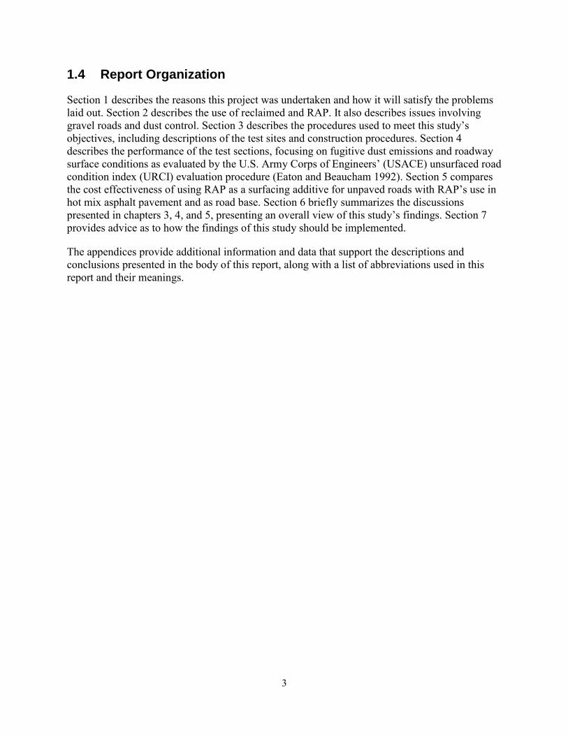
1.4 Report Organization Section 1 describes the reasons this project was undertaken and how it will satisfy the problems laid out. Section 2 describes the use of reclaimed and RAP. It also describes issues involving gravel roads and dust control. Section 3 describes the procedures used to meet this study’s objectives, including descriptions of the test sites and construction procedures. Section 4 describes the performance of the test sections, focusing on fugitive dust emissions and roadway surface conditions as evaluated by the U.S. Army Corps of Engineers’ (USACE) unsurfaced road condition index (URCI) evaluation procedure (Eaton and Beaucham 1992). Section 5 compares the cost effectiveness of using RAP as a surfacing additive for unpaved roads with RAP’s use in hot mix asphalt pavement and as road base. Section 6 briefly summarizes the discussions presented in chapters 3, 4, and 5, presenting an overall view of this study’s findings. Section 7 provides advice as to how the findings of this study should be implemented.

The appendices provide additional information and data that support the descriptions and conclusions presented in the body of this report, along with a list of abbreviations used in this report and their meanings.

5

2. LITERATURE REVIEW

2.1 Asphalt Pavement Reclamation and Recycling

Reclaimed or recycled asphalt pavement (RAP) is the term given to removed and/or reprocessed pavement materials containing asphalt and aggregates. These materials are obtained when asphalt pavements are removed for reconstruction, resurfacing, or to gain access to buried utilities. When properly crushed and screened, RAP consists of high-quality, well-graded aggregates coated by asphalt cement (FHWA 1998).

Asphalt pavement is the most recycled product in America today (Davio 1999). As a result, RAP is being used more widely throughout the world in various applications. Most of the RAP is put back into the roadways of America as a base or surface material. RAP is also used in embankment and fill applications throughout the industry. Another possible use is to utilize RAP in gravel roads.

Highways are a leading recycler—with more asphalt pavement recycled than any other product in America. Few people realize that highways are among the nation’s top recyclers. About 80% of asphalt pavement is being reused in the highway environment. That is compared with only 28% of recycled post-consumer goods in the municipal solid waste stream. In the transportation field, recycling is a win-win proposition. RAP saves the taxpayers’ dollars while maintaining high quality in the roadways of America. Recycling asphalt pavements also shows a healthy respect to the valuable materials used in asphalt pavements (AASHTO 2003).

According to industry experts, the asphalt pavement industry is the nation’s leader in recycling. Each year, 73 million tons of reclaimed asphalt pavements are reused, saving taxpayers almost $300 million annually. That is almost twice as much as paper, glass, plastic, and aluminum combined. The volume of recycled asphalt pavement is 13 times greater than recycling of newsprint, 27 times greater than recycling of glass bottles, 89 times greater than recycling of aluminum cans, and 267 times greater than recycling of plastic containers. Recycled asphalt is used not only for new roads, but also for roadbeds, shoulders, and embankments (AASHTO 2003).

The ownership of RAP can be broken down by contractor, agency, or a combination of the two. The State of Wyoming’s RAP is owned and controlled by an agency, most likely WYDOT. Colorado’s RAP is owned by both agencies and contractors. The sources of RAP include pavement milling, asphalt pavement removal, and plant waste material. RAP can either be stockpiled in isolated single source piles or as a blend of multiple sources. RAP can be processed in a number of ways, including screening, crushing, or fractioning (combination of both screening and crushing). RAP can also be processed into fine aggregate, minus ½ inch, or into coarse aggregate, greater than ½ inch (Huber 2008).

Asphalt pavement recycling has many advantages, including: • Reduced cost of construction • Conservation of aggregate and binders • Preservation of existing pavement geometrics

6

• Preservation of the environment • Conservation of energy

The use of hot-mix, hot in-place and cold in-place recycling achieves material and construction savings of up to 40%, 50% and 67%, respectively. In addition, significant user-cost savings are realized due to reduced interruption in traffic flow when compared with conventional rehabilitation techniques (Davio 1999).

2.2 Obtaining Reclaimed Asphalt Pavement

Asphalt pavement is generally removed either by milling or full-depth removal. Milling involves the removal of the pavement surface using a milling machine, which can remove up to 2 inches of (50 mm) thickness in a single pass. Full-depth removal involves ripping and breaking the pavement using a rhino horn on a bulldozer and/or pneumatic pavement breakers. In most instances, the broken material is picked up by front-end loaders and loaded into haul trucks. The material is then hauled to a central facility for processing. At this facility, the RAP is processed using a series of operations, including crushing, screening, conveying, and stacking (FHWA 1998).

Although the majority of old asphalt pavements are recycled at central processing plants, asphalt pavements may also be pulverized in place and incorporated into granular or stabilized base courses using a self-propelled pulverizing machine. Hot in-place and cold in-place recycling processes have evolved into continuous train operations that include partial depth removal of the pavement surface, mixing the reclaimed material with beneficiating additives (such as virgin aggregate, binder, and/or softening or rejuvenating agents to improve binder properties), and placing and compacting the resultant mix in a single pass (FHWA 1998).

2.3 Uses of Reclaimed Asphalt Pavement

The majority of the RAP that is produced is recycled and used, although not always in the same year that it is produced. RAP is almost always returned back into the roadway structure in some form, usually incorporated into asphalt paving by means of hot or cold recycling, but it is also sometimes used as an aggregate in base or sub-base construction (FHWA 1998).

It has been estimated that as much as approximately 33 million metric tons (36 million tons), or 80% to 85% of the excess asphalt concrete presently generated, is reportedly being used either as a portion of recycled hot mix asphalt, in cold mixes, or as aggregate in granular or stabilized base materials. Some of the RAP that is not recycled or used during the same construction season that it is generated is stockpiled and is eventually reused (FHWA 1998).

Milled or crushed RAP can be used in a number of highway construction applications. These include its use as an aggregate substitute and asphalt cement supplement in recycled asphalt paving (hot mix or cold mix), as a granular base or sub-base, as a stabilized base aggregate, or as an embankment or fill material. Recycled asphalt pavement can be used as an aggregate substitute material, but in this application it also provides an additional asphalt cement binder,

7

thereby reducing the demand for asphalt cement in new or recycled asphalt mixes containing RAP. When used in asphalt paving applications (hot mix or cold mix), RAP can be processed at either a central processing facility or on the job site (in-place processing). The introduction of RAP into asphalt paving mixtures is accomplished by either hot or cold recycling (FHWA 1998).

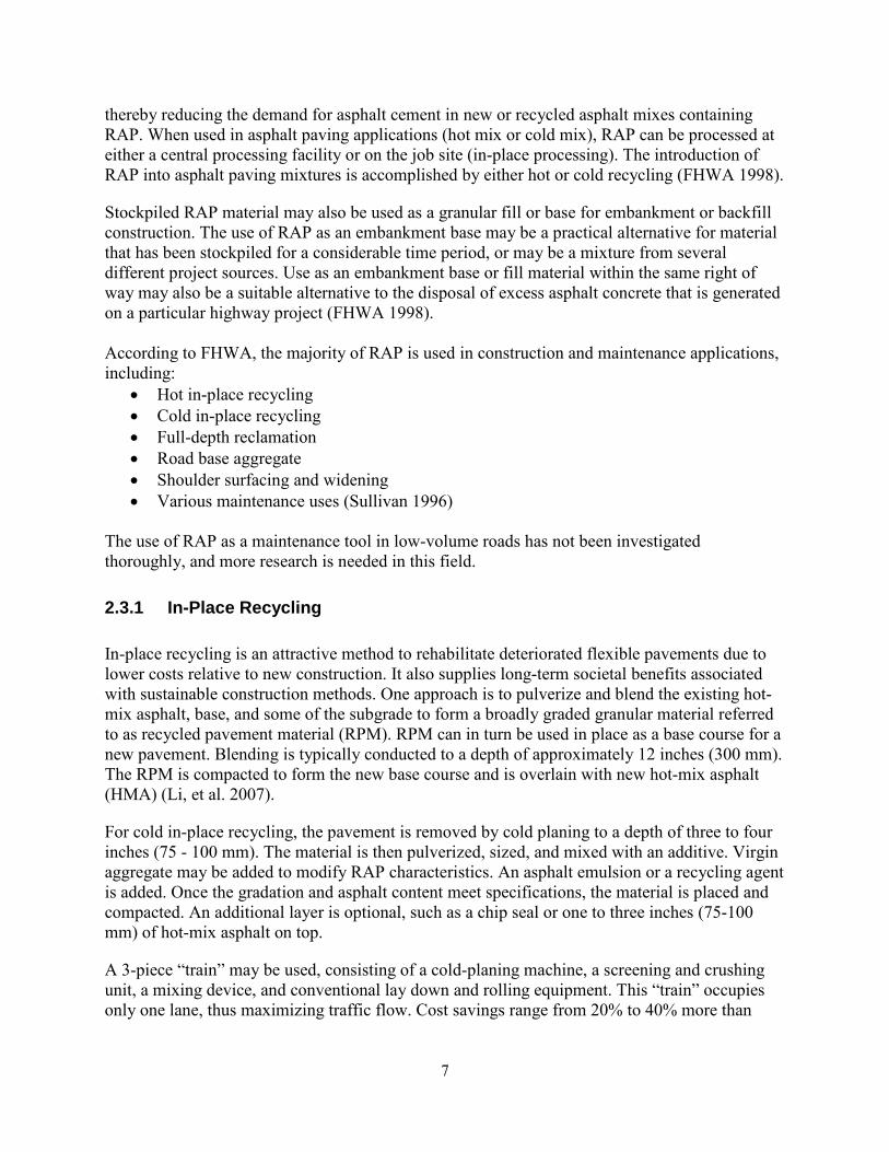
Stockpiled RAP material may also be used as a granular fill or base for embankment or backfill construction. The use of RAP as an embankment base may be a practical alternative for material that has been stockpiled for a considerable time period, or may be a mixture from several different project sources. Use as an embankment base or fill material within the same right of way may also be a suitable alternative to the disposal of excess asphalt concrete that is generated on a particular highway project (FHWA 1998). According to FHWA, the majority of RAP is used in construction and maintenance applications, including:

• Hot in-place recycling • Cold in-place recycling • Full-depth reclamation • Road base aggregate • Shoulder surfacing and widening • Various maintenance uses (Sullivan 1996)

The use of RAP as a maintenance tool in low-volume roads has not been investigated thoroughly, and more research is needed in this field.

2.3.1 In-Place Recycling

In-place recycling is an attractive method to rehabilitate deteriorated flexible pavements due to lower costs relative to new construction. It also supplies long-term societal benefits associated with sustainable construction methods. One approach is to pulverize and blend the existing hot-mix asphalt, base, and some of the subgrade to form a broadly graded granular material referred to as recycled pavement material (RPM). RPM can in turn be used in place as a base course for a new pavement. Blending is typically conducted to a depth of approximately 12 inches (300 mm). The RPM is compacted to form the new base course and is overlain with new hot-mix asphalt (HMA) (Li, et al. 2007).

For cold in-place recycling, the pavement is removed by cold planing to a depth of three to four inches (75 - 100 mm). The material is then pulverized, sized, and mixed with an additive. Virgin aggregate may be added to modify RAP characteristics. An asphalt emulsion or a recycling agent is added. Once the gradation and asphalt content meet specifications, the material is placed and compacted. An additional layer is optional, such as a chip seal or one to three inches (75-100 mm) of hot-mix asphalt on top.

A 3-piece “train” may be used, consisting of a cold-planing machine, a screening and crushing unit, a mixing device, and conventional lay down and rolling equipment. This “train” occupies only one lane, thus maximizing traffic flow. Cost savings range from 20% to 40% more than

8

conventional techniques. Since heat is not used, energy savings can be from 40% to 50% (Davio 1999).

For hot in-place recycling, the asphalt pavement is softened by heating, and is scarified or hot milled and mixed to a depth of ¾ to 1½ inches (19 - 37.5 mm). New hot-mix material (virgin aggregate and new binder) and/or a recycling agent is added in a single pass of a specialized machine in the “train.” A new wearing course may also be added with an additional pass after compaction (Davio 1999).

2.3.2 Hot Mix Asphalt and Reclaimed Asphalt Pavement (RAP)

At a central processing plant, RAP is combined with new hot aggregate and asphalt to produce asphalt concrete, using a batch or drum plant. The RAP is usually obtained from a cold-planing machine, but could also be from a ripping or crushing operation (Davio 1999). The result is hot-mix asphalt or HMA. The HMA is hauled from the plant to the project and compacted.

2.3.3 Cold Mix Asphalt (Central Processing Facility)

RAP processing requirements for cold-mix recycling are similar to those for recycled hot mix. However, the graded RAP produced is incorporated into cold-mix asphalt paving mixtures as an aggregate substitute (Davio 1999). The mix is then hauled to the project site and compacted.

2.3.4 Full Depth Reclamation

In the full-depth reclamation process, all the asphalt pavement section and a portion of the underlying materials are processed to produce a stabilized base course. The materials are crushed and additives are introduced. The materials are then shaped and compacted with the addition of a surface or wearing course that is applied on top (Davio 1999).

2.3.5 Embankment or Fill

FHWA’s “User Guidelines for Waste and By-product Materials in Pavement Construction” allows stockpiled RAP material to be used as a granular fill or base for embankment or backfill construction. RAP as an embankment base may be a practical alternative for material stockpiled for a considerable time period or that is a mixture from several project sources (Davio 1999) (FHWA 1998).

Research by the Florida Institute of Technology has found a new application for RAP material. RAP may be utilized as a stabilizing material for sub-base below rigid pavements, which will lead to increased use of RAP. RAP can also be used in embankment construction (Cosentino, Kalajian and Shieh 2003).

9

2.3.6 Mechanically Stabilized Earth Walls

Mechanically stabilized earth (MSE) walls have been used throughout the U.S. since the 1970s. The popularity of MSE systems is based on their low cost, aesthetic appeal, simple construction, and reliability. To ensure long-term integrity of MSE walls, select backfills consisting of predominantly of granular soils have been used. However, with increasing environmental and sustainability concerns, interest in the use of recycled materials for MSE walls has grown. Some of the most commonly available recycled materials are crushed concrete RAP, and these materials are being considered for use as backfill in MSE walls in Texas (Rathje, et al. 2006).

2.4 Economics of Reclaimed Asphalt Pavement (RAP)

RAP has been widely used in the United States since the 1970s and is a major benefit to the asphalt paving industry. The use of RAP allows for a lower mix material cost, elimination of the RAP disposal costs, and removal of a waste product from landfills. There are many additional benefits of using RAP, including:

• Recycling material that would otherwise be disposed of at the taxpayer’s expense, with a risk of harming the environment if disposed of improperly

• Maintaining original roadway geometrics • Lowering the initial cost of the pavement by utilizing recycled binder and aggregate,

which have a lower cost • No sacrifice in the mix performance when the RAP is handled and incorporated into the

mixture using the proper methods

A study completed in 1997 by the FHWA explains that some of the benefits of RAP are more than just cost savings. RAP saves room in landfills, transportation costs, and can be a better option under bridges and adjacent to guardrails where conventional overlays can be problematic (Kandhal 1997).

2.4.1 RAP in Hot Mix Asphalt

Recycling asphalt pavements is currently the largest single recycling practice in the United States. In 2002, 30 million tons of RAP was used in hot mix asphalt (HMA) with a savings of over $300 million, accomplished by lowering material costs for the newly placed asphalt and eliminating the disposal cost of the RAP (Putnam, Aune and Amirkhanian 2002).

Much of the literature consists of information and studies of RAP being reused in highway surfacing types of situations. There is much research pertaining to the benefits of using RAP in Hot Plant Mix and base. Many of the benefits of using RAP are described in an article entitled How to Maximize RAP Usage and Pavement Performance.

The use of reclaimed asphalt pavement (RAP) in new asphalt mixtures has many advantages to the environment, pavement owners, and contractors. Environmental benefits include a reduction of the carbon footprint of the product and any of its

10

end uses, conservation of landfill space, making asphalt paving an excellent sustainability practice.

From an economic standpoint, the use of RAP usually reduces the cost of the mix. In addition, the reuse of materials provides an opportunity to stabilize construction prices, which may fluctuate as the economy and demand for raw materials change.

Both the environmental and the economic benefits of recycling have been enhanced by new methods that allow using increased amounts of RAP in asphalt mixtures. Appropriately done, RAP mixtures can provide the same or better level of service than virgin asphalt mixtures (NAPA 2009).

With many economic, environmental, and durability benefits, RAP is an obvious choice for those DOTs and organizations that have access to it through either new construction or stockpile. The National Asphalt Pavement Association describes RAP as “a very valuable resource for the [Hot Mixed Asphalt] HMA producer.” It contains both aggregate and liquid asphalt. When RAP is used in HMA, it replaces both of these valuable resources, saving money and materials. Research has proven that recycled pavements offer the same durability as pavements constructed with 100% virgin materials, but with significant cost savings to the public and private consumer.

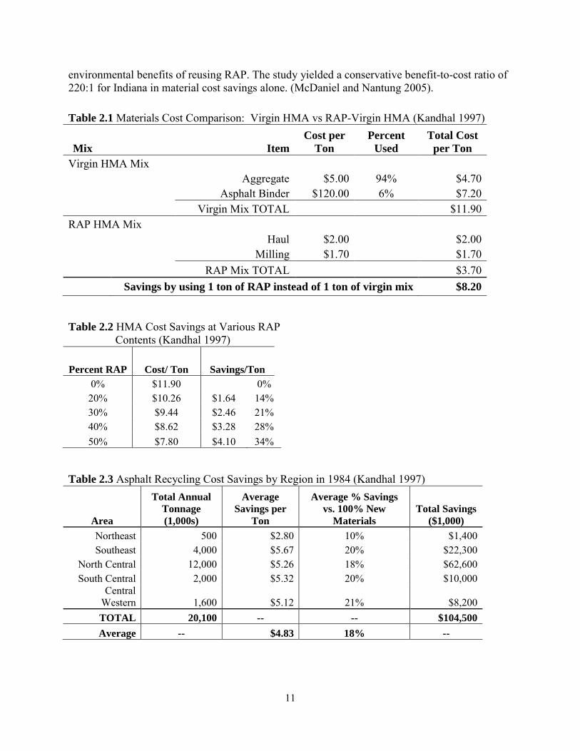
The FHWA report (Kandhal 1997) explains two approaches to determining the cost of using RAP, the material costs and the construction cost approaches. Table 2.1 shows the material cost approach. This example shows the amount of savings that can be achieved by using RAP instead of using virgin material. For example, consider $5 per ton and $120 per ton as average costs of aggregate and liquid asphalt, respectively. The cost of a 100% virgin mix with 6% asphalt comes out to be $11.90 per ton. If the contractor uses a half-lane milling machine and hauls the RAP back to the HMA plant, the total cost for RAP is $3.70 per ton, considering $1.70 per ton for machine and labor milling, and $2.00 per ton for trucking costs. Hence, the savings, compared with using virgin aggregate material, is $8.20 per ton. Table 2.2 shows the savings when using different percentages of RAP. It should be noted that these savings are in initial cost. A typical cost savings with hot mix recycling is shown in Table 2.3 for different regions within the United States. All cost analysis tables were obtained from the FHWA report entitled Pavement Recycling Guidelines for State and Local Governments (Kandhal 1997).

Financial considerations are a significant part of decisions regarding the use of RAP. Several states have conducted studies to determine if the use of RAP in hot plant mixes is cost effective and the results are overwhelming. The Florida DOT estimates $224 million in savings from the use of RAP since 1979, the equivalent of two thirds of their annual resurfacing budget. A Minnesota study estimated 18% savings if 40% RAP were used in HMA production (Horvath 2003). The Indiana DOT conducted a cost–benefit analysis of a research project (Designing Superpave Mixes with Locally Reclaimed Asphalt Pavement) as part of an independent review of the cost-effectiveness of the DOT’s research program. According to the conservative estimate of the cost-effectiveness review, Indiana DOT’s savings in materials were nearly $330,000 per year when adding only 5% RAP to more than 5 million tons of base and intermediate mixes—although RAP contents of 15% to 20% are more typical. The review did not assess the

11

environmental benefits of reusing RAP. The study yielded a conservative benefit-to-cost ratio of 220:1 for Indiana in material cost savings alone. (McDaniel and Nantung 2005).

Table 2.1 Materials Cost Comparison: Virgin HMA vs RAP-Virgin HMA (Kandhal 1997)

Mix Item Cost per

Ton Percent

Used Total Cost

per Ton Virgin HMA Mix

Aggregate $5.00 94% $4.70

Asphalt Binder $120.00 6% $7.20

Virgin Mix TOTAL $11.90 RAP HMA Mix

Haul $2.00

$2.00

Milling $1.70 $1.70

RAP Mix TOTAL

$3.70

Savings by using 1 ton of RAP instead of 1 ton of virgin mix $8.20

Table 2.2 HMA Cost Savings at Various RAP Contents (Kandhal 1997)

Percent RAP Cost/ Ton Savings/Ton 0% $11.90

0%

20% $10.26 $1.64 14% 30% $9.44 $2.46 21% 40% $8.62 $3.28 28% 50% $7.80 $4.10 34%

Table 2.3 Asphalt Recycling Cost Savings by Region in 1984 (Kandhal 1997)

Area

Total Annual Tonnage (1,000s)

Average Savings per

Ton

Average % Savings vs. 100% New

Materials Total Savings

($1,000) Northeast 500 $2.80 10% $1,400 Southeast 4,000 $5.67 20% $22,300

North Central 12,000 $5.26 18% $62,600 South Central 2,000 $5.32 20% $10,000

Central Western 1,600 $5.12 21% $8,200 TOTAL 20,100 -- -- $104,500 Average -- $4.83 18% --

12

2.4.2 RAP in Road Base

A research study on blending RAP into road base was done by Sultan Qaboos University in the Sultanate of Oman, where recycling of pavement materials is not practiced. However, in 1995, the Ministry of Communication tested the recycling of old asphalt materials as a base layer. The results of a laboratory study conducted at Sultan Qaboos University indicated that RAP aggregate could be expected to replace virgin aggregate in road subbases if RAP is mixed with other virgin aggregates (Taha, et al. 2002). However, minimal use of RAP (only 10%) could be utilized in road base construction.

Laboratory and field evaluations of the use of RAP in road base and subbase applications were also conducted by Rutgers University (Maher and Popp 1997). Results of this study showed that RAP has a slightly higher resilient modulus and field elastic modulus than the dense-graded aggregate used in the State of New Jersey. RAP base potential was also evaluated by constructing the Lincoln Avenue demonstration project in 1993 in Urbana, Illinois (Garg and Thompson 1996). Laboratory and field experiences indicated that RAP could be successfully used as a conventional base material. Field performance was comparable to that of a crushed stone base.

2.5 Unpaved Roads

In the United States, 53% of all the roads are unpaved. That translates into over 1.6 million miles of unpaved roadways, most of which are gravel roads (Skorseth and Selim 2000). The definition of gravel by the South Dakota LTAP and the FHWA is “a mix of stone, sand, and fine-sized particles used as a subbase, base or surfacing on a road. In some regions, it may be defined as ‘aggregate.’”

Gravel roads generally provide lower service to the user and are usually considered inferior to paved roads. For the most part, gravel roads exist to provide access or service. In many cases, gravel roads will not be paved due to the very low traffic volumes and/or not having the funds to adequately improve the subbase and base and then pave the road (Henning, Bennett and Kadar 2007).

Gravel roads are abundant in America and especially in Wyoming. These roads are used by industry, farming, ranching, and tourism. The majority of problems that exist on gravel roads are the result of dust loss and the associated distresses. A possible additive to gravel roads is RAP. The addition of RAP may address dust loss and the associated problems. Whether used alone or in conjunction with other dust suppressants, RAP may provide an economical treatment for agencies fighting to keep dust loss at a minimum.

In other nations throughout the world, unpaved roads, generally gravel, make up most of the road network. They are used by farmers and ranchers to get their product in and out of their fields; by the timber industry to get equipment in and product out of forests; and by the mining and oil industries to get to and from their sites with equipment and product. Gravel roads are also used to access remote areas like lakes or campgrounds as well as providing rural residents access to their homes.

13

Two basic principles can make or break a gravel road. The grading device(s) and the surface gravel are the most important elements in a well maintained or rehabilitated gravel road. The grader is used to properly shape the road to provide for adequate drainage of water. The volume and quality of the gravel aggregate is most likely more important to the roadway than the grader. For instance, corrugations or “washboarding” is more likely caused by the material itself and less likely by the grader, although this is generally perceived by the public in an opposite fashion (Skorseth and Selim 2000).

The change in the vehicles and equipment using low volume gravel roads is another matter of importance. The size of trucks and agricultural equipment are increasing, and the effect of the larger and heavier loads on gravel roads is just as serious as the effect on paved roads.

2.5.1 Gravel Road Distresses

There are seven types of distresses that can be characterized by a surface evaluation on a gravel road. The seven distresses are:

• Improper cross section • Inadequate roadside drainage • Corrugations • Dust • Potholes • Ruts • Loose aggregate

These distresses are established by the U.S. Army Corps of Engineers Cold Regions Research and Engineering Laboratory (Eaton and Beaucham 1992).

Another methodology that involves the same distresses in a different fashion is the Gravel PASER Manual. PASER stands for Pavement Surface Evaluation and Rating. This publication by the Transportation Information Center at the University of Wisconsin-Madison assesses gravel roadway conditions based on five roadway conditions. These five conditions involve the same distress as the U.S. Army Corps of Engineers approach but group them differently. The five conditions include:

• Crown The height and condition of the crown, and an unrestricted slope of roadway from the center across the shoulders to the ditches

• Drainage The ability of roadside ditches and under-road culverts to carry water away from the road

• Gravel Layer Adequate thickness and quality of gravel to carry the traffic loads

• Surface Deformations Washboarding, potholes, ruts

• Surface Defects Dust and loose aggregate (Walker, Entine and Kummer 2002)

14

In whatever methodology used to evaluate gravel roads, the underlying distresses are the keys to the chosen procedure. Either approach is considered viable and is in the choice of the agency maintaining the roadway. Both methodologies have their own individual rating system based on the distresses present in the roadway. In any case, it is the distresses that will convey the quality of the gravel road. Keep in mind, the surface conditions of gravel roads can change overnight by means of heavy precipitation and local traffic. The aforementioned distresses will be described in more detail in the following subsections.

2.5.1.1 Cross-Section and Crown

The shape of entire roadway must be understood in order to properly maintain gravel roads. To properly maintain these roads, three basic roadway characteristics must be understood: a crowned driving surface, a shoulder area that slopes away from the driving surface, and a ditch. Generally, these three items must be correct in the road’s cross section or a gravel road will not perform well, even under very low traffic. The shape of the roadway is the responsibility of the agency and equipment operators who are in charge of the road. The shape of the road surface and shoulders is classified as routine maintenance.

The cross section of a gravel road is designed to drain all water away from the roadway. Gravel roads tend to rut in wet weather. In fact, standing water at any place in the cross section is one of the major reasons for surface distresses and the failure of a gravel road. The agency in charge of maintaining the road must do everything possible in their routine maintenance to take care of the roadway’s shape or else extra equipment and manpower may have to be brought in to rehabilitate the road, which generally is not in the budget. Also, a well maintained roadway shape will serve low volume traffic well, but when heavy loads are introduced, the roadway may fail due to weak subgrade strengths and low gravel depths (Skorseth and Selim 2000).

2.5.1.2 Drainage

Roadside ditches and culverts must be able to handle surface water flow. When water is ponding, it is the result of poor roadside drainage. Sitting water on the roadway will seep into the layers below and soften the road base. Ditches need to be wide and deep enough to accommodate all of the surface water. When ditches and culverts are not in good enough condition due to improper shape or maintenance, water will not be directed properly, resulting in ponding and water backup. The shape of the ditch may be affected by erosion and repairs may be necessary. Erosion control efforts may be needed to help maintain ditches. Also, buildups of debris in the ditches or culverts need to be removed as part of routine maintenance. Any roadway material in the ditch may be placed back on the roadway or hauled away (Eaton and Beaucham 1992) (Walker, Entine and Kummer 2002).

2.5.1.3 Gravel Layer

There is a need for an adequate layer of gravel-based traffic loads. It is in the gravel layer in which the traffic loads are carried and distributed to the subsoils. The thickness of the gravel layer is dependent on the amount of heavy traffic and the stability of the soils below. Generally,

15

a minimum of 6 inches (150 mm) is required. Layers used for heavier loads or poor subsoils can be as much as 10 inches (250 mm) or more. Not only does the volume of the gravel layer matter but the quality of the gravel being used. It is in the quality in which good, long-term service will be prevalent. The use of the word quality in this context refers to the gradation and durability of the gravel. These are measured by hardness and soundness testing. In general, the proper gradation has a good mix of larger aggregate, sand-sized aggregate, and fines. Gradation and quality of the gravel is based on agency specifications and can widely vary (Walker, Entine and Kummer 2002).

2.5.1.4 Surface Deformations

Surface deformations include corrugations, potholes, and ruts. Washboarding or corrugations are closely spaced ridges and valleys or ripples at fairly regular intervals. Corrugation is the result of traffic dislodging aggregate from the roadway surface. These ripples develop perpendicular to the direction of travel. Where heavy traffic and loose aggregate are present, corrugations tend to occur. They also usually form on hills and curves, at intersections, where accelerating and decelerating by traffic is present, and around areas where the surface is soft or potholed. Soft subgrades and improper grading can also result in washboarding. When washboarding is severe, water can become trapped in the valleys and more problems can occur.

Potholes are bowl-shaped depressions that can develop in the gravel or on the surface. Potholes are created when traffic wears away small pieces of the surface or where soft spots are developing in the underlying layers. Pothole growth is accelerated when water collects in the hole. As a result of the sitting water, the roadway continues to get worse because of more material becoming loose and/or more soft spots in the subbase form. Small isolated potholes can be fixed by hand. Moderate and severe potholes need the use of a grader and more aggregate to be fixed.

Ruts are surface depressions that usually form in the wheel path of the road. Rutting develops parallel to the road’s centerline and can occur anywhere along the width of the driven road surface. Some ruts may be caused by the dislodging of the surface gravel while others occur with the permanent deformation in any of the road layers or subgrade. Repeated vehicle passes over soft spots in the road results in rutting. Poor crown and drainage can weaken the underlying soils and help accelerate the formation of ruts. Significant rutting can destroy a road (Eaton and Beaucham 1992) (Walker, Entine and Kummer 2002).

2.5.1.5 Surface Defects

Surface defects include dust and loose aggregate. When the road is dry, traffic can create dust. The wear and tear on the gravel roads by the traffic loads will eventually loosen the larger aggregate from the soil binder or the fines. These fines are then picked up by the traffic and become airborne. Dust can create poor visibility for trailing vehicles and is considered an air pollutant. It is important to replace these fines to maintain the roadway. Most of the time, fines can be reclaimed from the shoulder and remixed into the existing surface.

16

Loose aggregate is the result of the wear and tear on the roadway that causes the fines to be lost in the form of dust. When the fines are lost, loose aggregate develops on the surface and/or the shoulder. Generally, the action of the traffic will move the loose gravel to the center or edges of the roadway. Loose aggregate can also form where vehicles tend to turn around or stop. The loose aggregate on the road and the fines from the road’s edge may be able to be remixed by a grader to recreate a well-graded gravel and be reused (Eaton and Beaucham 1992).

2.5.2 Dust Control

There are strong reasons to control dust from unpaved roads. The main problem associated with unpaved roads is fugitive dust created by traffic and the loss of fines. Dust is considered as a type of particulate matter air pollution. It can contaminate houses and barns; it settles on vegetation and can reduce visibility over long distances. Dust is usually kicked up into the air by vehicles or blown off the road by wind. When dust is blown away, aggregates in the road surface loosen, which can lead to many types of distresses and costly maintenance or rehabilitation efforts, as well as higher road user costs in the form of vehicle maintenance (Kuennen 2006) (Addo, Sanders and Chenard 2004).

Dust control methods range from spraying the road with chemicals to using geotextiles in the reconstruction of a road. Other efforts may include reduction in vehicular speed and the application of water. The use of dust suppressants is justifiable when traffic is low and paving is not a feasible option financially; the cost of the suppressants and application are low when stage construction is planned. Commonly used dust suppressants are water, chloride compounds, lignin derivatives, and resinous adhesives. Performance characteristics, as well as the type and volume of traffic, climate, roadway conditions, and product cost, all play a significant role in selecting a dust suppressant (Addo, Sanders and Chenard 2004) (Sanders and Addo, Effectiveness and Environmental Impact of Road Dust Suppressants 1993) (Sanders 1993). A study conducted in Wyoming by Koch in 2010 maintains that dust reduction through the use of RAP is very significant, up to 41%, with no change in serviceability to the gravel surface.

There are strong reasons to control dust from unpaved roads. The top problem associated with unpaved roads is fugitive dust created by traffic and the loss of fines. Dust is considered a type of particulate matter air pollution. It can contaminate houses and barns, it settles on vegetation, and can reduce visibility over long distances. Dust is usually kicked up into the air by vehicles or blown off the road by wind. Not only is dust present on gravel roads, it is also generated by road construction and is a given at quarries and gravel pits. Also, as more dust leaves the road surface, the less road surface remains. When dust is blown away, aggregates in the road surface loosen, which can lead to many types of distresses and costly maintenance or rehabilitation efforts for road departments, as well as higher road user costs in the form of vehicle maintenance (Kuennen 2006) (Addo, Sanders and Chenard 2004).

Dust is considered a coarse particle (PM-10), that is, dust is made up of particles that are 10 micrometers (microns) or less. Another way look at it is dust particles are about one-seventh of the diameter of a human hair. The USEPA has had national air quality standards for PM-10 since 1987. These standards consist of a 24-hour standard not to exceed 150 micrograms per cubic

17

meter of air, and an average standard of 50 micrograms per cubic meter annually (Kuennen 2006).

Scientific studies have linked particulate matter pollution with significant health problems such as:

• Increased respiratory symptoms like irritation of airways, coughing, and difficulty breathing

• Decreased lung function • Aggravated asthma • Development of chronic bronchitis • Irregular heartbeat • Premature death of people with heart or lung disease

Coughing, wheezing, and decreased lung function in healthy individuals can be caused by particle pollution (Kuennen 2006).

The standards for dust exclude dust that occurs due to natural kick-up by the wind. It is not practical or feasible to place regulation on dust caused by the wind. On the other hand, it is possible to manage fugitive dust with dust control measures (Kuennen 2006).

2.5.2.1 Types of Dust Suppressants

Dust control methods range from spraying the road with chemicals to using geotextiles in the reconstruction of a road. Other efforts may include reduction in vehicular speed and the application of water. The use of dust suppressants is justifiable when traffic is low and paving is not a feasible option financially, the cost of the suppressants and application are low, and when stage construction is planned. The commonly used dust suppressants are water, chloride compounds, lignin derivatives, and resinous adhesives. Performance characteristics as well as the type and volume of traffic, climate, roadway conditions, and product cost all play a significant role in selecting a dust suppressant (Addo, Sanders and Chenard 2004) (Sanders and Addo 1993).

The main idea behind dust suppression is to keep moisture in the surface of the roadway. Moisture keeps the dust particles wet, which in turn increases their mass and cohesion. The moisture allows fines in the gravel to adhere to other fines as well as other aggregate in the mix. When the moisture content is sufficient, optimum compaction under the traffic load is achieved (Kuennen 2006).

2.5.2.1.1 Water

Fresh or sea water is the oldest dust suppressant used. It is readily available, although in the semi-arid West it is a commodity, and applied by spraying onto the road surface. The service capacity of water is limited and temporary due to evaporation. Excess watering may create undesirable runoff being the cause for potential erosion and excessive mud. Several light applications of water are preferred over one heavy application. Although water may be less

18

expensive as a product, the money saved will be consumed by the frequency of applications and labor costs (Addo, Sanders and Chenard 2004) (Kuennen 2006).

2.5.2.1.2 Chloride Compounds

Road mangers should consider chloride stabilization as a cost-effective method of dust control and other maintenance applications on gravel roads. Calcium chloride (CaCl2) and magnesium chloride (MgCl2) are the most commonly used chloride compounds. Sodium chloride (NaCl) is also sparingly used and is the least effective (Addo, Sanders and Chenard 2004). These chlorides can be used by themselves or combined with other additives to create various types of product.

The desired effect of chloride compounds lies in their physical properties. Chlorides are hygroscopic, which means they can attract and absorb moisture from the atmosphere and retain it for extended periods of time. The result is a road surface that is constantly damp. The chloride properties are closely related to relative humidity and air temperature. A relative humidity of 30% to 40% is the point where calcium chloride and magnesium chloride stop attracting and absorbing moisture from the atmosphere. Also, another characteristic contained in chloride compounds is their low freezing points depending on concentration in a liquid solution. This results in reduced effects from the freeze-thaw cycles and minimized frost heaves, which can cause gravel roads to weaken (Monlux and Mitchell 2006).

Chloride compounds are reasonably simple to use and have additional benefits such as improved ride, reduced sedimentation in streams, reduced aggregate loss, reduced inhalation hazards, reduced vehicle maintenance, and increased safety. These compounds are water soluble and can be washed out during wet weather cycles (Skorseth and Selim 2000).

2.5.2.1.3 Lignin Derivatives

Industrial waste products, animal fats, and vegetable oils make up these suppressants. The most common lignin derivative used is lignin sulfonate, a waste byproduct from the paper milling industry. Some personnel in the field refer to it as “tree sap.” It is said that lignin is the natural cement that holds the wood fibers of plants together. When the pulping process occurs, lignin polymers and wood sugars are released into the processing wastewater. The wastewater is referred to as lignin sulfonate. When used as a suppressant, the lignin polymers act as a binder for the soil particles. This keeps the dust particles glued together and they become harder to get airborne. Lignin sulfonate is water soluble and can be washed away during wet weather conditions (Addo, Sanders and Chenard 2004) (Skorseth and Selim 2000).

2.5.2.1.4 Resinous Adhesives

These dust suppressants include byproducts from the plastic industry, waste oils, tars, and bitumen. The most widely used products are cutback asphalt and asphalt emulsions. Cutback asphalts are the result of a solvent added to asphalt cement. Different cutbacks are produced based on the type of solvent used. Rapid-curing cutback is the result of using highly volatile solvents such as gasoline or naptha. Medium and slow-curing cutbacks are created when lighter

19

solvents such as kerosene are used. Asphalt emulsions are created by dispersing asphalts as small droplets of water. This is achieved by adding an emulsifying agent during the process. When resinous adhesives are used as dust suppressants, they create the most durable, dust-free surfaces. This is due to their high cohesive properties and their insolubility to water. The use of these products was once popular, but the amount of fuel oil or kerosene in these products, along with rising fuel costs, has resulted in declined use and is being banned in many places. These products need to be applied by special asphalt application equipment (Addo, Sanders and Chenard 2004).

2.5.2.1.5 Clay

Clays have also been used as dust suppressants. Clays have high plasticity and strong cohesion and work well when added to gravel in the right proportions. It is hard to haul and mix clay with gravel due to its high plasticity. For tars and bitumens, the structure and composition of the aggregates is the major factor that affects their cohesion in aggregate-asphalt mixes. A byproduct of soybean oil refining is also used as a dust suppressant. It is biodegradable and has many characteristics of light petroleum-based oils. This product will penetrate the surface and create a light bond that reduces dust. There are also many other commercial products that may be used and should be tested on small sections of roadway before full use is decided upon (Skorseth and Selim 2000).

2.5.3 Dust Collection and Measurement

A majority of the research done with dust measurements has been focused in atmospheric pollution. Within the study of atmospheric pollution, dust measurements focus on two areas: 1) atmospheric modeling and prediction and 2) field measurement and quantification. The three main methods of air sampling techniques used by atmospheric pollution scientists are classified as sedimentation techniques, filtration techniques, and photometric techniques (Sanders and Addo 2000).

The sedimentation technique is a sampling method used for dust particle fallout from the atmosphere. These techniques follow ASTM D 1739 standards. Open-top containers, such as glass, metal, or plastic jars are used in this method. These containers have a height that is two to three times the diameter of the jar. Particulates are collected over an exposure period that is typically a month. The collected amount of particulate is expressed in terms of weight per unit area per 30 days. This technique depends on the forces of gravity and limits the particle size to about 2 µm or greater. There are a number of disadvantages to this technique as it requires an extended collection period for one sample, contaminated samples caused by foreign matter mixing with the collected dust, and the effect of winds on the samples (Sanders and Addo 2000).

The filtration technique employees the use of a suction source under a filter. The type of filter and the sampling equipment is dependent on the desired data and type of test being performed. An example of a device that uses the filtration technique is the high volumetric sampler. The major drawback of this technique is that it requires the use of electric power to run the suction pump (Sanders and Addo 2000).

20

The photometric technique is based on the absorption properties of particulates passing through a light source. Basically, this technique looks at the light scattering as a sample passes through a light source. The amount of light scattered is dependent on the concentration, size, refractive index, shape, and color of the suspended particles.

The devices and techniques developed to measure road dust employ one or more of these particulate sampling techniques. In 1972, the USDA’s Forest Service used the photometric technique to measure dust concentrations at a point along an unpaved road (Wellman and Barraclough 1972). Research performed in Iowa used the sedimentation technique by installing cups on the roadside of unpaved roads to gain data on the nature of dust generation and distribution (Hoover, et al. 1973). In 1984, the USDA’s Forest Service built a portable cyclone dust collector and mounted it on the rear of a dust-generating vehicle (Langdon 1984). The goal of this research was to use the filtration technique over a section of the road versus one point on the road. In 1986, the USDA Forest Service in a cooperative study at Cornell University (Irwin, Taylor and Aneshanlsley 1986) developed a device that measured the road dust in terms of air opacity using photometric techniques. This device was called the Road Dust Monitor.

Between 1992 and 1995, a Mountain-Plains Consortium and Department of Transportation sponsored research project was undertaken by Thomas Sander and Jonathan Addo at Colorado State University. One objective of this project was to develop an inexpensive dust measuring device. Due to problems associated with the roadside bucket method of dust collection, a decision was made to develop a device to measure dust production from test sections that mounted on a vehicle and took real-time measurements. Modeling a device similar to the Langdon device (Langdon 1984), the Colorado State University Dustometer was created. The device and method were developed to generate quantitative and reproducible measurements that could be used to directly measure the dust mass in the field (Sanders and Addo 2000).

2.6 Literature Review Summary

RAP plays a significant role in the recycling world and in the highway environment, yet productive use of this material on gravel roads has remained limited. There is no significant research into the use of RAP on gravel roads but it has the potential to provide an option in the fight to reduce dust loss and maintain roadway serviceability. Given the large amount of RAP that is produced in Wyoming and the quantity of gravel roads, there is justification for further research into the use of RAP on gravel roads.

Fugitive dust emissions and roadway surface conditions are two primary characteristics of unpaved roads. Any treatment, material, or process used on these roads needs to both provide an adequate driving surface and minimize dust emissions, both for safety and environmental reasons. Methods of assessing and monitoring surface conditions and dust emissions are described.

21

3. METHODOLOGY

Reclaimed asphalt pavement (RAP) test sections in Laramie, Johnson and Sweetwater Counties were constructed and monitored from 2008 through 2011. Various construction and treatment methods were used on the test sections. Materials and construction data were collected, along with traffic and other environmental data. The sections’ performances were monitored for surface conditions and fugitive dust emissions.

3.1 Test Section Descriptions

Sections of Laramie County’s Atlas Road [CR 224] and Pry Road [CR 124] (see Figure 3.1) north of Cheyenne; Johnson County’s Schoonover Road [CR 204B] (see Figure 3.2) east of Buffalo; and Sweetwater County’s Crooks Gap Road [CR 23] (see Figure 3.3) just north of Wamsutter were constructed and evaluated. Figure 3.4 shows that each of these sections are located near an interstate highway, which was each section’s RAP source, as well as the source of much of their traffic. Abbreviations used to describe the sections are in Appendix E.

Figure 3.1 Laramie County test sites

22

Figure 3.2 Johnson County test site

Figure 3.3 Sweetwater County test site

23

Figure 3.4 Wyoming test site locations

3.1.1 Site Layouts

3.1.1.1 Laramie County Test Sections Layout

The Laramie County site consisted of three sections on Atlas Road [CR 224], two of which had RAP added and a third control section that had only the original surfacing aggregate (see Figure 3.5), and two sections on Pry Road [CR 124], one with RAP and a control section with only the original surfacing (see Figure 3.6). The characteristics of these five sections, placed in April 2008, are summarized in Table 3.1.

3.1.1.2 Johnson County Test Sections Layout

The Johnson County site on Schoonover Road [CR 204B] consists of three sections, one with a RAP and aggregate blend, one with a RAP and aggregate blend and calcium chloride, and one with aggregate and calcium chloride. The test sections begin once the road leaves the state right-of-way, with the first mile receiving the aggregate-RAP blend. The half-mile surfaced with this RAP blend nearest I-90 did not receive any further treatment, while the half-mile further from I-90 was treated with calcium chloride, as was the next half-mile of existing aggregate surfaced road. These three sections, placed in June 2008, are described in Table 3.2 and shown in Figure 3.7.

24

Figure 3.5 Laramie County Atlas Road test sections.

Figure 3.6 Laramie County Pry Road test sections.

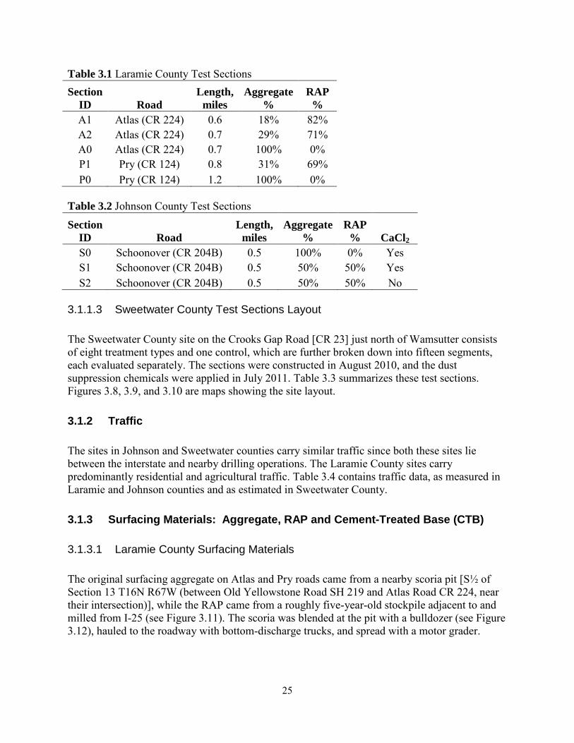
25

Table 3.1 Laramie County Test Sections Section

ID Road Length,

miles Aggregate

% RAP

% A1 Atlas (CR 224) 0.6 18% 82% A2 Atlas (CR 224) 0.7 29% 71% A0 Atlas (CR 224) 0.7 100% 0% P1 Pry (CR 124) 0.8 31% 69% P0 Pry (CR 124) 1.2 100% 0%

Table 3.2 Johnson County Test Sections

Section ID Road

Length, miles

Aggregate %

RAP % CaCl2

S0 Schoonover (CR 204B) 0.5 100% 0% Yes S1 Schoonover (CR 204B) 0.5 50% 50% Yes S2 Schoonover (CR 204B) 0.5 50% 50% No

3.1.1.3 Sweetwater County Test Sections Layout

The Sweetwater County site on the Crooks Gap Road [CR 23] just north of Wamsutter consists of eight treatment types and one control, which are further broken down into fifteen segments, each evaluated separately. The sections were constructed in August 2010, and the dust suppression chemicals were applied in July 2011. Table 3.3 summarizes these test sections. Figures 3.8, 3.9, and 3.10 are maps showing the site layout.

3.1.2 Traffic

The sites in Johnson and Sweetwater counties carry similar traffic since both these sites lie between the interstate and nearby drilling operations. The Laramie County sites carry predominantly residential and agricultural traffic. Table 3.4 contains traffic data, as measured in Laramie and Johnson counties and as estimated in Sweetwater County.

3.1.3 Surfacing Materials: Aggregate, RAP and Cement-Treated Base (CTB)

3.1.3.1 Laramie County Surfacing Materials

The original surfacing aggregate on Atlas and Pry roads came from a nearby scoria pit [S½ of Section 13 T16N R67W (between Old Yellowstone Road SH 219 and Atlas Road CR 224, near their intersection)], while the RAP came from a roughly five-year-old stockpile adjacent to and milled from I-25 (see Figure 3.11). The scoria was blended at the pit with a bulldozer (see Figure 3.12), hauled to the roadway with bottom-discharge trucks, and spread with a motor grader.

26

Figure 3.7 Johnson County test sections on Schoonover Road, JO CR 204B.

27

Figure 3.8 Sweetwater County test segments on Crooks Gap Road,

SW CR 23, south end.

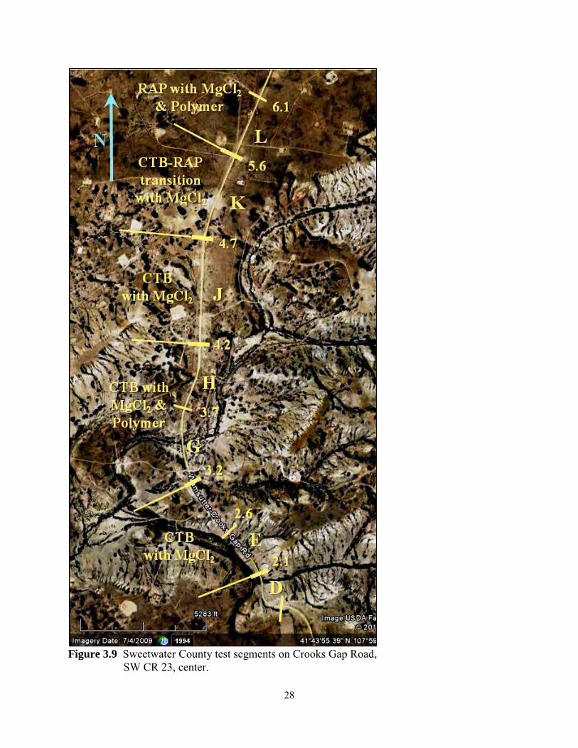
28

Figure 3.9 Sweetwater County test segments on Crooks Gap Road,

SW CR 23, center.

29

Figure 3.10 Sweetwater County test segments on Crooks

Gap Road, SW CR 23, north end.

30

Table 3.3 Sweetwater County Test Sections

Table 3.4 Approximate Test Section Traffic Volumes and Speeds

Section ID Road

Begin Mile

End Mile

Length, miles

Surfacing Material§

Dust Control Agent¤

Dust Control Rate,

gallons/yd2

A Crooks Gap [CR 23] 0.0 0.5 0.5 CB M --B Crooks Gap [CR 23] 0.5 1.1 0.6 CB M --C Crooks Gap [CR 23] 1.1 1.6 0.5 CB LM 0.5D Crooks Gap [CR 23] 1.6 2.1 0.5 CB LM 0.5E Crooks Gap [CR 23] 2.1 2.6 0.5 CTB M 0.5F Crooks Gap [CR 23] 2.6 3.2 0.6 CTB M 0.5G Crooks Gap [CR 23] 3.2 3.7 0.5 CTB PM 0.4H Crooks Gap [CR 23] 3.7 4.2 0.5 CTB PM 0.4J Crooks Gap [CR 23] 4.2 4.9 0.7 CTB M 0.5K Crooks Gap [CR 23] 4.9 5.6 0.7 CTB-RAP M 0.5L Crooks Gap [CR 23] 5.6 6.1 0.5 RAP PM 0.3M Crooks Gap [CR 23] 6.1 6.6 0.5 RAP PM 0.3N Crooks Gap [CR 23] 6.6 7.2 0.6 RAP M 0.5P Crooks Gap [CR 23] 7.2 7.6 0.4 RAP None --Q Crooks Gap [CR 23] 7.6 8.0 0.4 RAP None --

§ CB: WYDOT Grading W crushed base; CTB: milled cement-treated base; RAP: milled reclaimed asphalt pavement; CTB-RAP inconsistent blend of milled CTB and RAP

¤ M: MgCl2 brine; LM: lignin sulfonate blended half-and-half with MgCl2; PM: MgCl2 blended half-and-half with a proprietary polymer

County RoadVehicles per Day

% Trucks

85th percentile

speed, mph

LA Atlas (CR 224) 50 3% 55LA Pry (CR 124) 50 12% 56JO Schoonover (CR 204B) 188 74% 51SW Crooks Gap (CR 23) 300 35% 50

31

Figure 3.11 Laramie County material source locations.

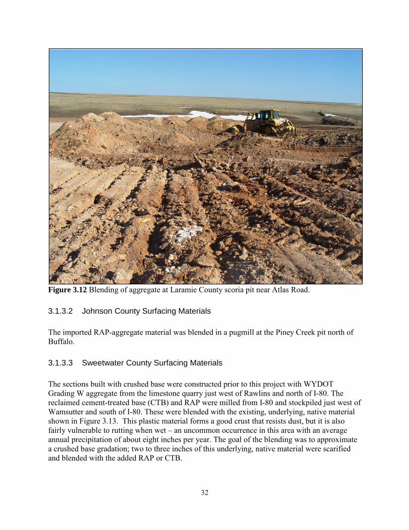
32

Figure 3.12 Blending of aggregate at Laramie County scoria pit near Atlas Road.

3.1.3.2 Johnson County Surfacing Materials

The imported RAP-aggregate material was blended in a pugmill at the Piney Creek pit north of Buffalo.

3.1.3.3 Sweetwater County Surfacing Materials

The sections built with crushed base were constructed prior to this project with WYDOT Grading W aggregate from the limestone quarry just west of Rawlins and north of I-80. The reclaimed cement-treated base (CTB) and RAP were milled from I-80 and stockpiled just west of Wamsutter and south of I-80. These were blended with the existing, underlying, native material shown in Figure 3.13. This plastic material forms a good crust that resists dust, but it is also fairly vulnerable to rutting when wet – an uncommon occurrence in this area with an average annual precipitation of about eight inches per year. The goal of the blending was to approximate a crushed base gradation; two to three inches of this underlying, native material were scarified and blended with the added RAP or CTB.

33

Figure 3.13 Crooks Gap Road north of the test sections showing the surfacing material typical

of that which was blended with RAP or CTB on the Sweetwater County test sections.

3.1.4 Dust Suppression Agents

3.1.4.1 Johnson County Calcium Chloride

The treated sections on Schoonover Road received calcium chloride pellets. The pellets were spread on the dampened roadway surface, and additional water was placed on the roadway after the calcium chloride was placed as described in section 3.3.2 below.

3.1.4.2 Sweetwater County Magnesium Chloride and Blends

The control sections with crushed base were treated with magnesium chloride brine on June 28, 2011, and earlier—at least three weeks before the other dust control agents were applied. The various sections treated with dust suppressants July 19-21, 2011, received the types of agents shown in Table 3.3 at the rates shown therein. Application methods are described below in section 3.3.3.

34

3.2 Testing Methods

3.2.1 Aggregate

3.2.1.1 Gradations

Aggregate gradation tests with and without a wash analysis were performed according to AASHTO standards T 27 and T 11.

3.2.1.2 Plastic and Liquid Limits

Liquid and plastic limit tests were performed according to AASHTO standards T 89 and T 90.

3.2.1.3 In-Situ Moisture Contents

Moisture sampling consisted of collecting a sample of the top ½ to 1 inch of the road surface. A small section of the roadway’s surface was removed with a pick or spade. The sample was placed in a tin sampling can and sealed with tape to prevent moisture transfer. The samples were weighed, dried to a constant weight in an oven set at 105⁰C, and re-weighed to get the water weight and dry weight. Moisture content was calculated by taking the water weight and dividing it by the dry weight.

3.2.2 Weather

Wind speed, direction, and temperature were recorded with a WindMate 200 by Speedtech Industries when dust measurements were taken.

3.2.3 Dust Assessment

3.2.3.1 Dustometer

Dust monitoring was performed using the Colorado State University (CSU) dustometer. The dustometer is a dust collection device that attaches behind the driver side rear wheel of the test vehicle. The dustometer is an inexpensive moving dust sampler that was developed at CSU by Thomas Sanders and Jonathan Addo. It has been proven to be a quantitative, reproducible, and precise device for dust measurement (Sanders and Addo 1993).

The device consists of a fabricated steel filter box that contains glass microfiber filters; a standard high volumetric suction pump; a steel mounting bracket attached to the bumper of the test vehicle; a flexible hose for connecting the suction pump to the filter box; a gas-powered generator; an on/off switchbox for the suction pump; and a 2001 Chevy Suburban used as a testing vehicle. The steel filter box has an opening facing the rear wheel covered with a 200 µm mesh sieve screen (150 μm [#100] on the Sweetwater County segments) that prevents large

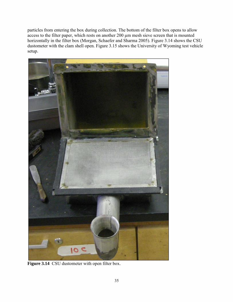
35

particles from entering the box during collection. The bottom of the filter box opens to allow access to the filter paper, which rests on another 200 µm mesh sieve screen that is mounted horizontally in the filter box (Morgan, Schaefer and Sharma 2005). Figure 3.14 shows the CSU dustometer with the clam shell open. Figure 3.15 shows the University of Wyoming test vehicle setup.

Figure 3.14 CSU dustometer with open filter box.

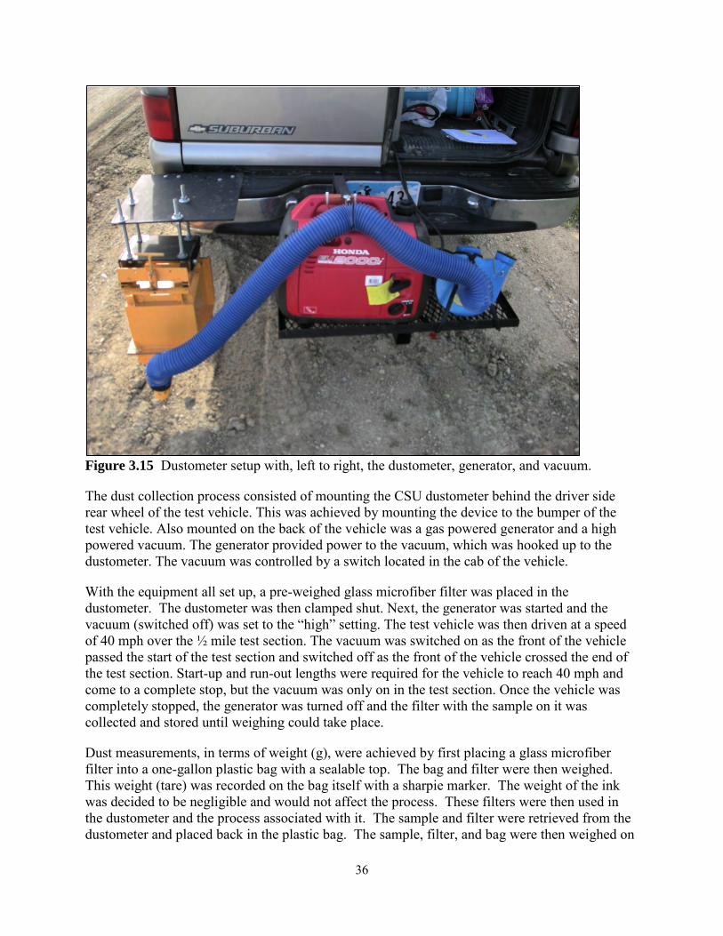
36

Figure 3.15 Dustometer setup with, left to right, the dustometer, generator, and vacuum.

The dust collection process consisted of mounting the CSU dustometer behind the driver side rear wheel of the test vehicle. This was achieved by mounting the device to the bumper of the test vehicle. Also mounted on the back of the vehicle was a gas powered generator and a high powered vacuum. The generator provided power to the vacuum, which was hooked up to the dustometer. The vacuum was controlled by a switch located in the cab of the vehicle.

With the equipment all set up, a pre-weighed glass microfiber filter was placed in the dustometer. The dustometer was then clamped shut. Next, the generator was started and the vacuum (switched off) was set to the “high” setting. The test vehicle was then driven at a speed of 40 mph over the ½ mile test section. The vacuum was switched on as the front of the vehicle passed the start of the test section and switched off as the front of the vehicle crossed the end of the test section. Start-up and run-out lengths were required for the vehicle to reach 40 mph and come to a complete stop, but the vacuum was only on in the test section. Once the vehicle was completely stopped, the generator was turned off and the filter with the sample on it was collected and stored until weighing could take place.

Dust measurements, in terms of weight (g), were achieved by first placing a glass microfiber filter into a one-gallon plastic bag with a sealable top. The bag and filter were then weighed. This weight (tare) was recorded on the bag itself with a sharpie marker. The weight of the ink was decided to be negligible and would not affect the process. These filters were then used in the dustometer and the process associated with it. The sample and filter were retrieved from the dustometer and placed back in the plastic bag. The sample, filter, and bag were then weighed on

37

the same scale and a gross weight was recorded. The difference in the gross and tare weight (net weight) resulted in the weight of dust collected for that particular section. This weight was divided by the length of the test section, yielding a dust measurement in grams per mile.

3.2.3.2 Visual and Photographic Assessments

Numerous photographs were taken. Surface and dust conditions were noted throughout construction and monitoring of the various test sections.

3.2.4 Roadway Condition Evaluations: URCI

Surface distresses of each section were evaluated using the methods presented in Unsurfaced Road Maintenance Management developed by the USACE (Eaton and Beaucham 1992). A representative subsection of each test section was established and marked for monitoring. Each subsection was walked and each individual distress was rated and recorded according to the USACE methods and a total unsurfaced road condition index (URCI) was calculated.

3.3 Construction Methods

3.3.1 Laramie County: Blade Mixed

RAP was applied to the Atlas and Pry Road sections in Laramie County using the following procedure:

1) Water applied to surface 2) Surface scarified to a depth of 2 to 3 inches with rippers mounted on a motor grader (see

Figure 3.16) 3) RAP placed in a windrow with bottom-discharge trucks (see Figure 3.17) 4) RAP and scarified aggregate blended and spread with a motor grader (see Figures 3.18

and 3.19) 5) Road shape and crown re-established with a motor grader 6) Compacted by traffic

38

Figure 3.16 Scarifying Laramie County’s Atlas Road prior to placement and blending of RAP.

Figure 3.17 Placement of RAP windrow on Laramie County’s Atlas Road with bottom-

discharge haul trucks.

39

Figure 3.18 Blending RAP and existing, scarified aggregate on Laramie

County’s Atlas Road.

Figure 3.19 Blending and shaping RAP and existing, scarified aggregate on Laramie County’s

Atlas Road.

40

3.3.2 Johnson County: Stockpile Mixed

RAP was applied to Schoonover Road using the following procedure: 1) RAP and aggregate blended half-and-half in a pugmill at the Piney Creek stockpiles (see

Figure 3.20). 2) Existing roadway shaped with a motor grader (see Figure 3.21). 3) RAP-aggregate hauled to the roadway and placed in windrows with bottom-discharge

trucks (see Figure 3.22). 4) RAP-aggregate blend shaped with a motor grader (see Figure 3.23). 5) Water applied to aid compaction. 6) RAP-aggregate blend compacted with motor grader tires and pneumatic compactors

mounted to the ripper hydraulics (see Figure 3.24). 7) Final compaction with a single steel drum roller (see Figure 3.25).

Calcium chloride pellets were applied as follows:

1) The roadway was dampened with a water truck. 2) Calcium chloride pellets were applied to the roadway (see Figures 3.26 and 3.27). 3) Additional water was applied to hold down the calcium chloride pellets. 4) Pellets worked into surface by traffic (see Figures 3.28 and 3.29).

Figure 3.20 RAP and virgin aggregate stockpiles at Johnson County’s Piney Creek stockpiles,

June 2008.

41

Figure 3.21 Initial shaping of Johnson County’s Schoonover Road prior to placement

of the blended RAP and aggregate, June 2008.

Figure 3.22 Placing RAP and aggregate blend on Johnson County’s Schoonover Road,

June 2008.

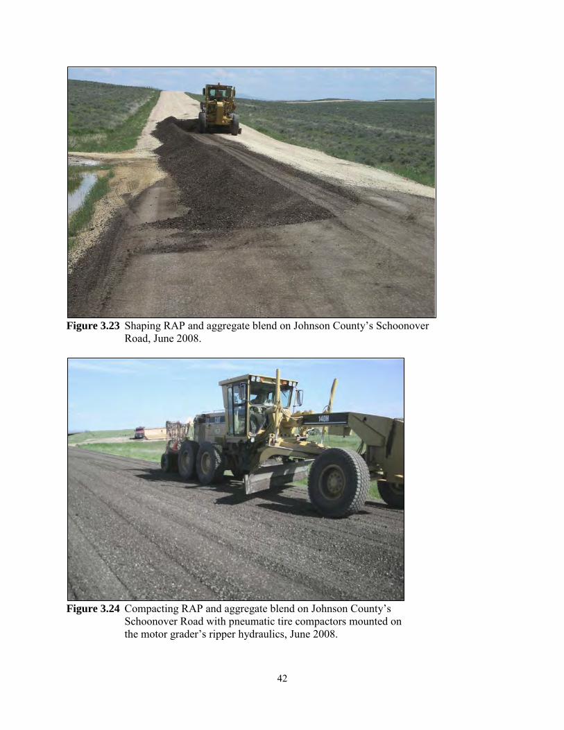
42

Figure 3.23 Shaping RAP and aggregate blend on Johnson County’s Schoonover

Road, June 2008.

Figure 3.24 Compacting RAP and aggregate blend on Johnson County’s

Schoonover Road with pneumatic tire compactors mounted on the motor grader’s ripper hydraulics, June 2008.

43

Figure 3.25 Final compaction of the RAP aggregate blend on

County”s Schoonover Road, June 2008.

Figure 3.26 Calcium chloride flakes placed on damp RAP and aggregate

blend on Johnson County’s Schoonover Road, June 2008.

44

Figure 3.27 Close-up of calcium chloride flakes on Johnson County’s

Schoonover Road, June 2008.

Figure 3.28 Calcium chloride flakes partially worked into the aggregate

surface by traffic on Johnson County’s Schoonover Road, June 2008.

45

Figure 3.29 Calcium chloride flakes mostly worked into the aggregate

surface by traffic on Johnson County’s Schoonover Road, June 2008.

3.3.3 Sweetwater County: Reclaimer Mixed

The RAP and cement-treated base (CTB) were applied to the Crooks Gap Road sections as follows:

1) Existing surface scarified to several inches. 2) CTB and/or RAP hauled to roadway and placed with bottom-discharge trucks. 3) RAP or CTB spread with a motor grader. 4) RAP or CTB blended with underlying, scarified existing aggregate with a Caterpillar

RM-500 Rotary Mixer reclaimer (see Figure 3.30). 5) Blended material wetted with water trucks (see Figure 3.31), shaped with motor graders

(see Figure 3.32), and compacted with pneumatic tired roller attached to ripper mounts (see Figure 3.33).

46

Figure 3.30 Operation of the reclaimer used to blend the underlying, existing surface with RAP

or CTB on Sweetwater County’s Crooks Gap Road. (1) Adjustable rear door. (2) Universal rotor. (3) Breaker bars. (4) Adjustable front door.

Figure 3.31 Applying water to the CTB and aggregate blend prior to final shaping

and compaction on Sweetwater County’s Crooks Gap Road, August 2010.

47

Figure 3.32 Blending and shaping the existing aggregate and CTB blend on

Sweetwater County’s Crooks Gap Road, August 2010.

Figure 3.33 Final shaping and compaction of CTB and aggregate blend using a

motor grader with pneumatic tire compactors mounted to its ripper hydraulics on Sweetwater County’s Crooks Gap Road, August 2010.

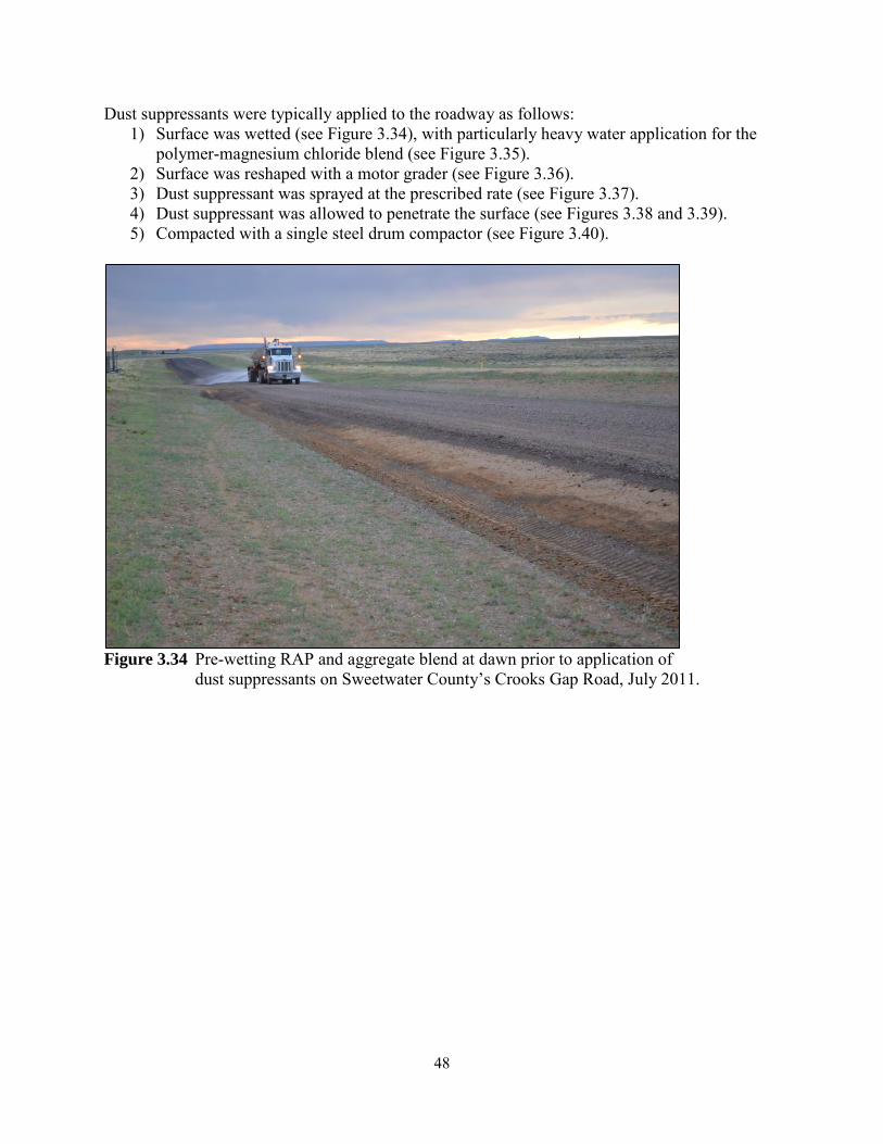
48

Dust suppressants were typically applied to the roadway as follows: 1) Surface was wetted (see Figure 3.34), with particularly heavy water application for the

polymer-magnesium chloride blend (see Figure 3.35). 2) Surface was reshaped with a motor grader (see Figure 3.36). 3) Dust suppressant was sprayed at the prescribed rate (see Figure 3.37). 4) Dust suppressant was allowed to penetrate the surface (see Figures 3.38 and 3.39). 5) Compacted with a single steel drum compactor (see Figure 3.40).

Figure 3.34 Pre-wetting RAP and aggregate blend at dawn prior to application of

dust suppressants on Sweetwater County’s Crooks Gap Road, July 2011.

49

Figure 3.35 Dampened aggregate and RAP blend prepared

for application of magnesium chloride and polymer dust suppressant on Sweetwater County’s Crooks Gap Road, July 2011.

Figure 3.36 Shaping dampened RAP and aggregate blend in preparation for

placement of dust suppressants on Sweetwater County’s Crooks Gap Road, July 2011.

50

Figure 3.37 Applying dust suppressant brine to aggregate and RAP blend on

Sweetwater County’s Crooks Gap Road, July 2011.

Figure 3.38 Recently applied magnesium chloride on the RAP and aggregate blend

on Sweetater County’s Crooks Gap Road, July 2011.

51

Figure 3.39 Magnesium chloride almost completely absorbed into the RAP and

aggregate blend on Sweetwater County’s Crooks Gap Road, July 2011.

Figure 3.40 Compaction of the magnesium chloride-treated RAP and aggregate blend

on Sweetwater County’s Crooks Gap Road, July 2011.

52

3.4 Summary of Methodologies

Test sections were established in Laramie, Johnson, and Sweetwater counties. These sections were established to evaluate the performance of RAP and in some cases, dust suppressants, on fugitive dust emissions and surface performance of unpaved roads. Construction methods are described. Test methods evaluating the materials, fugitive dust emissions, and roadway surface conditions are described.

The Laramie County sections on Pry and Atlas roads, CR 124 and CR 224, were constructed with RAP from I-25 hauled in from a nearby stockpile and blended with a motor grader. Three test sections with RAP blended with the existing aggregate were constructed, as were two control sections without RAP.

Three sections were constructed on Johnson County’s Schoonover Road, CR 204B. Two were surfaced with a 1:1 stockpile blend of virgin aggregate and RAP. One of these and an adjacent section without RAP were treated with calcium chloride flakes.

Nine sections, further broken down into 15 segments, were constructed on Sweetwater County’s Crooks Gap Road, CR 23. Surfacing materials consisted of WYDOT Grading W crushed limestone base and blends of the existing, native aggregate with cement-treated base (CTB) or RAP. Most were treated with one of three types of magnesium chloride-based dust suppressant, while two segments were constructed with a RAP blend but were not treated with any dust suppressant.

53

4. RESULTS

Evaluations of fugitive dust emissions assessment methods begin this section. Comparisons between visual, subjective observations of dust emissions based on the USACE unsurfaced road condition index (URCI) method (Eaton and Beaucham 1992) and the quantitative measurements made with the CSU dustometer (Sanders and Addo 2000) are made. The effects of various environmental factors on the results achieved with the dustometer are evaluated.

All of the three counties’ sections are evaluated, describing their performances as functions of materials, maintenance, and construction methods. These evaluations consist of four elements: materials properties, visual observations including photographs, the URCI, and dust emissions.

4.1 Visual Dust Ratings vs Dustometer Measurements

On the Sweetwater County test sites, both visual dust ratings and measurements with the dustometer were performed. To assess what measured values in grams per mile correspond to visual ratings on a scale of None/Low/Medium/High dust as described by the USACE (Eaton and Beaucham 1992), Figure 4.1 plots the None, Low, Medium, and High sections on a full scale, while Figure 4.2 plots the measured values for the None, Low, and Medium visually rated sections on a partial scale. For this dustometer setup (50 psi tires, ½ ton truck [Chevy Suburban], and #100 [150 μm] pre-screen), the suggested ranges in grams per mile for each of the four visual classifications are as shown in Figure 4.2, with cutoffs at 0.15, 0.40, and 1.00 grams per mile. Though there is some variance from these values, this provides some correlation between the measured values generated with the dustometer and the visual descriptions provided by Eaton and Beaucham. This correlation is summarized in Table 4.1.

54

Figure 4.1 Dust measured with the dustometer as a function of subjective visual dust ratings,

with a suggested numerical cutoff between Medium and High dust severity at 1.00 grams per mile.

0

1

2

3

4

5g/

mile

Visual Dust Rating

Non

e

Low

Med

ium

Hig

h

Medium/High cutoff @ 1.00 g/mi

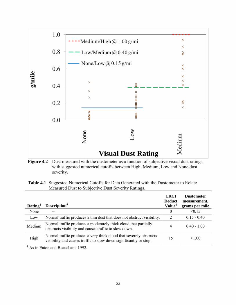
55

Figure 4.2 Dust measured with the dustometer as a function of subjective visual dust ratings,

with suggested numerical cutoffs between High, Medium, Low and None dust severity.

Table 4.1 Suggested Numerical Cutoffs for Data Generated with the Dustometer to Relate Measured Dust to Subjective Dust Severity Ratings.

Rating§ Description§

URCI Deduct Value§

Dustometer measurement, grams per mile

None -- 0 <0.15 Low Normal traffic produces a thin dust that does not obstruct visibility. 2 0.15 - 0.40

Medium Normal traffic produces a moderately thick cloud that partially obstructs visibility and causes traffic to slow down. 4 0.40 - 1.00

High Normal traffic produces a very thick cloud that severely obstructs visibility and causes traffic to slow down significantly or stop. 15 >1.00

§ As in Eaton and Beaucham, 1992.

0.0

0.2

0.4

0.6

0.8

1.0g/

mile

Visual Dust Rating

Non

e

Low

Med

ium

Medium/High @ 1.00 g/mi

None/Low @ 0.15 g/mi

Low/Medium @ 0.40 g/mi

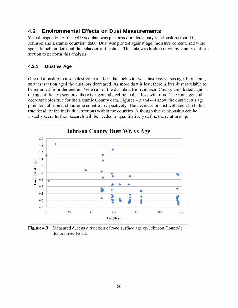
56

4.2 Environmental Effects on Dust Measurements Visual inspection of the collected data was performed to detect any relationships found in Johnson and Laramie counties’ data. Dust was plotted against age, moisture content, and wind speed to help understand the behavior of the data. The data was broken down by county and test section to perform this analysis.

4.2.1 Dust vs Age

One relationship that was desired to analyze data behavior was dust loss versus age. In general, as a test section aged the dust loss decreased. As more dust is lost, there is less dust available to be removed from the section. When all of the dust data from Johnson County are plotted against the age of the test sections, there is a general decline in dust loss with time. The same general decrease holds true for the Laramie County data. Figures 4.3 and 4.4 show the dust versus age plots for Johnson and Laramie counties, respectively. The decrease in dust with age also holds true for all of the individual sections within the counties. Although this relationship can be visually seen, further research will be needed to quantitatively define the relationship.

Figure 4.3 Measured dust as a function of road surface age on Johnson County’s Schoonover Road.

57

Figure 4.4 Measured dust as a function of road surface age on Laramie County’s Atlas and Pry Roads.

4.2.2 Dust vs Moisture Content

The dust loss and moisture content relationship was also investigated. It was concluded that no particular relationship between dust loss and moisture content in the individual sections can be established. This is because dust data were not collected when the roadway surface was wet. This resulted in a small range of moisture contents in which dust was collected. Also, within the small range of moisture contents there are no big variations in the collected dust weights. These conclusions hold true for both Johnson and Laramie counties. Figures 4.5 and 4.6 give examples of dust loss versus moisture content in Johnson and Laramie counties, respectively. Additional data are shown in Appendix A.

4.2.3 Dust vs Wind Speed

The relationship between dust loss and wind speed was also desired. It was suggested from visual inspection that a general trend between dust loss and wind speed could be inferred. The higher the wind speed, the lower the collected dust weight. Examples of this can be seen in Figures 4.7 and 4.8 for Johnson and Laramie counties, respectively. It should also be noted that the variability in the dust weights is most likely attributed to the wind direction with respect to the direction of travel. That is, a strong headwind would force more dust into the collection box while a strong tailwind would prevent dust from reaching the box. It is suggested that dust collection should not be performed in high winds in order to ensure fair sampling.

58

Figure 4.5 Measured dust as a function of moisture content on Johnson County’s

Schoonover Road, section S2 with RAP/aggregate blend and no calcium chloride.

Figure 4.6 Measured dust as a function of moisture content on Laramie County’s

Atlas Road, section A1 with blended RAP and existing aggregate.

59

Figure 4.7 Measured dust as a function of wind speed on Johnson County’s

Schoonover Road, section S2 with RAP and aggregate surfacing but no calcium chloride.

Figure 4.8 Measured dust as a function of wind speed on Laramie County’s Pry

Road, section S1 with blended RAP and existing aggregate.

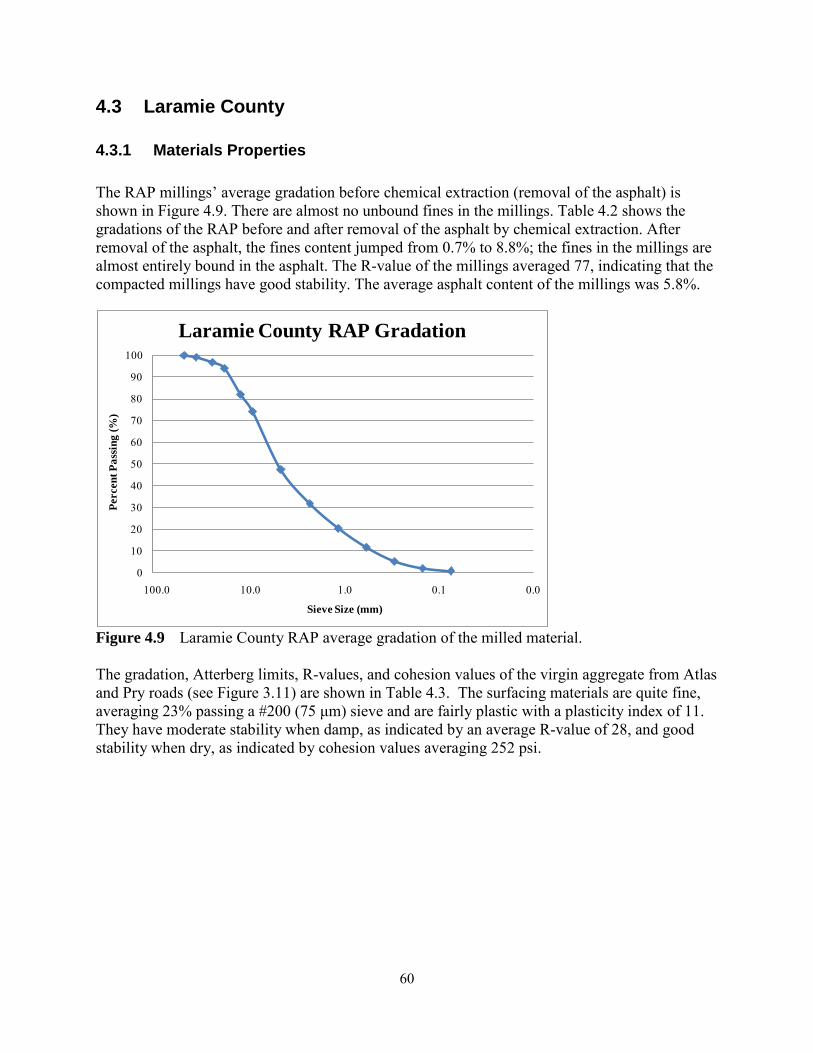
60

4.3 Laramie County

4.3.1 Materials Properties

The RAP millings’ average gradation before chemical extraction (removal of the asphalt) is shown in Figure 4.9. There are almost no unbound fines in the millings. Table 4.2 shows the gradations of the RAP before and after removal of the asphalt by chemical extraction. After removal of the asphalt, the fines content jumped from 0.7% to 8.8%; the fines in the millings are almost entirely bound in the asphalt. The R-value of the millings averaged 77, indicating that the compacted millings have good stability. The average asphalt content of the millings was 5.8%.

Figure 4.9 Laramie County RAP average gradation of the milled material. The gradation, Atterberg limits, R-values, and cohesion values of the virgin aggregate from Atlas and Pry roads (see Figure 3.11) are shown in Table 4.3. The surfacing materials are quite fine, averaging 23% passing a #200 (75 μm) sieve and are fairly plastic with a plasticity index of 11. They have moderate stability when damp, as indicated by an average R-value of 28, and good stability when dry, as indicated by cohesion values averaging 252 psi.

0

10

20

30

40

50

60

70

80

90

100

0.00.11.010.0100.0

Perc

ent P

assi

ng (%

)

Sieve Size (mm)

Laramie County RAP Gradation

61

Table 4.2 Laramie County RAP Materials Test Results

A2 A1 P1 Average2 in. (50.8 mm) 100.0 100.0 100.0 100.0

1 1/2 in. (38.1 mm) 97.9 99.5 100.0 99.11 in. (25.4 mm) 94.7 97.4 98.3 96.8

3/4 in. (19.0 mm) 92.3 94.5 95.8 94.21/2 in. (12.7 mm) 80.0 82.3 83.5 81.93/8 in. (9.5 mm) 72.1 74.4 75.8 74.1No. 4 (4.75 mm) 44.2 48.0 49.8 47.3No. 8 (2.38 mm) 32.5 33.3 29.6 31.8No. 16 (1.19 mm) 22.1 21.9 16.9 20.3No. 30 (0.595 mm) 13.3 13.3 8.5 11.7No. 50 (0.297 mm) 5.9 6.8 3.0 5.2No. 100 (0.149 mm) 2.2 2.8 1.0 2.0No. 200 (0.075 mm) 0.8 0.9 0.4 0.7

Sample A Sample B Sample C AverageR - Value 76.0 77.0 79.0 77.3

% Oil 5.85 5.59 5.88 5.77

Sample A Sample B Sample C Average3/4 in. (19.0 mm) 100.0 100.0 100.0 100.01/2 in. (12.7 mm) 93.3 91.7 92.3 92.43/8 in. (9.5 mm) 88.4 84.4 88.0 86.9No. 4 (4.75 mm) 63.5 60.3 63.9 62.6No. 8 (2.38 mm) 47.5 44.6 48.3 46.8No. 16 (1.19 mm) 36.3 33.9 36.5 35.6No. 30 (0.595 mm) 27.8 25.9 27.6 27.1No. 50 (0.297 mm) 20.0 18.6 19.8 19.5No. 100 (0.149 mm) 13.4 12.5 13.5 13.1No. 200 (0.075 mm) 8.9 8.3 9.3 8.8

RAP WindrowSieve SizePercent Passing After Oil Extraction

Laramie County - Atlas and Pry Roads

Sieve SizePercent PassingRAP Windrow

62

Table 4.3 Laramie County Virgin Aggregate Materials Test Results

Table 4.4 contains test results from samples taken from the RAP and virgin aggregate road surface blends. Table 4.5 shows interpolations to empirically determine the RAP percentage as constructed based on asphalt contents and percentages passing the #200 (75 μm) sieve. Since one would expect greater variability in the fines content than the asphalt content, the values from the asphalt content are assumed to be closest to ‘correct,’ as shown in Figure 3.1. Interestingly, the R-values of the blends were almost identical to those of the RAP alone, averaging only 1 less – 76 vs 77 – and they were much higher than the virgin aggregate alone which had R-values averaging 28.

Atlas Pry Average1 1/2 in. (38.1 mm) 100.0 100.0 100.0

1 in. (25.4 mm) 99.8 99.4 99.63/4 in. (19.0 mm) 99.4 98.6 99.01/2 in. (12.7 mm) 97.6 96.4 97.03/8 in. (9.5 mm) 95.3 93.7 94.5No. 4 (4.75 mm) 78.1 76.1 77.1No. 8 (2.38 mm) 65.1 65.1 65.1No. 16 (1.19 mm) 54.8 57.7 56.2No. 30 (0.595 mm) 45.2 49.7 47.4No. 50 (0.297 mm) 35.4 40.1 37.7

No. 100 (0.149 mm) 29.3 32.7 31.0No. 200 (0.075 mm) 22.4 23.6 23.0

Atlas Pry AverageLiquid Limit (LL) 26.5 27.0 26.8

Plasticity Index (PI) 11.5 11.0 11.3Cohesion Value (CV) psi 340.5 164.0 252.3Fractured Faces (FF) %

R - Value 30.0 26.0 28.0% Gravel 0.3 0.0 0.2% Sand 62.4 60.2 61.3% Silt 23.2 26.5 24.9% Clay 14.2 13.8 14.0

Laramie County - Atlas and Pry RoadsPercent Passing

100 % Gravel Control

Insuffcient Material

Sieve Size

63

Table 4.4 Laramie County Surface Blended Materials Test Results

A2 A1 P1 Average3 in. (76.2 mm) 100.0 100.0 100.0 100.02 in. (50.8 mm) 100.0 99.5 100.0 99.8

1 1/2 in. (38.1 mm) 100.0 99.5 100.0 99.81 in. (25.4 mm) 98.4 98.8 99.2 98.8


A2 A1 P1 AverageR - Value 78.0 73.0 78.0 76.3

% Oil 4.18 4.61 4.07 4.29

A2 A1 P1 Average1 in. (25.4 mm) 100.0 100.0 100.0 100.0


Percent Passing After Oil ExtractionRAP Blended SurfaceSieve Size

Laramie County - Atlas and Pry Roads

Sieve SizePercent Passing

RAP Blended Surface

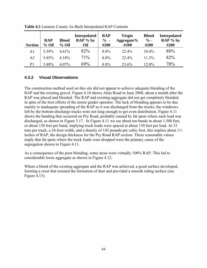
64

Table 4.5 Laramie County As-Built Interpolated RAP Contents

Section RAP

% Oil Blend % Oil

Interpolated RAP % by

Oil

RAP % -#200

Virgin Aggregate%

-#200

Blend % -#200

Interpolated RAP % by

#200 A1 5.59% 4.61% 82% 8.8% 22.4% 10.4% 88% A2 5.85% 4.18% 71% 8.8% 22.4% 11.3% 82% P1 5.88% 4.07% 69% 8.8% 23.6% 12.0% 78%

4.3.2 Visual Observations

The construction method used on this site did not appear to achieve adequate blending of the RAP and the existing gravel. Figure 4.10 shows Atlas Road in June 2008, about a month after the RAP was placed and blended. The RAP and existing aggregate did not get completely blended, in spite of the best efforts of the motor grader operator. The lack of blending appears to be due mainly to inadequate spreading of the RAP as it was discharged from the trucks; the windrows left by the bottom-discharge trucks were not long enough to get even distribution. Figure 4.11 shows the banding that occurred on Pry Road, probably caused by fat spots where each load was discharged, as shown in Figure 3.17. In Figure 4.11 we see about ten bands in about 1,500 feet, or about 150 feet per band, implying truck loads were spaced at about 150 feet per load. At 33 tons per truck, a 24-foot width, and a density of 145 pounds per cubic foot, this implies about 1½ inches of RAP, the design thickness for the Pry Road RAP section. These reasonable values imply that fat spots where the truck loads were dropped were the primary cause of the segregation shown in Figure 4.11.

As a consequence of the poor blending, some areas were virtually 100% RAP. This led to considerable loose aggregate as shown in Figure 4.12.

Where a blend of the existing aggregate and the RAP was achieved, a good surface developed, forming a crust that resisted the formation of dust and provided a smooth riding surface (see Figure 4.13).

65

Figure 4.10 Segregation of RAP on Laramie County’s Atlas Road in June 2008, two months after initial RAP application.

Figure 4.11 Segregation bands attributed to inadequate spreading of the windrows placed by the bottom-discharge haul trucks on Laramie County’s Pry Road in November 2008, six months after initial application.

66

Figure 4.12 Nearly 100% RAP resulting in excessive loose aggregate on Laramie County’s Atlas Road in June 2008, about two months after initial application.

Figure 4.13 Well compacted, tight surface due to good blending on Laramie

County’s Atlas Road in June 2008, about two months afetr initial application.

67

The Laramie County RAP sections were re-worked with a motor grader in August 2008, three months after the RAP was placed, due to the segregation (see Figure 4.14). Two months later, most of the RAP section had a good surface (see Figure 4.15), though some areas still had areas of nearly 100% RAP that set up hard, while adjacent spots exhibited a better, more thoroughly blended surface (see Figure 4.16).

Figure 4.14 Re-working Laramie County’s Pry Road in August 2008, four months after initial

application, to correct segregation with additional blending and spreading.

Both control sections generally performed well, as shown in Figures 4.17 and 4.18, with loose aggregate generally being the primary distress.

68

4.3.3 Unsurfaced Road Condition Index (URCI)

URCI ratings were performed on all five Laramie County sections nine times between June 24, 2008, and October 4, 2008. These ratings are plotted in Figure 4.19. Both control sections were rated excellent for all nine rating events; the Pry Road control section, P0, exhibited no measureable distresses; the Atlas Road control section, A0, exhibited only minor loose aggregate; and section A2, the eastern RAP section on Atlas Road, the middle of the Atlas Road section, had only loose aggregate as a measurable distress. The Pry Road RAP section, P1, was generally in excellent condition, except for the last rating in October when loose aggregate and rutting combined to give it a very good rating. The western RAP section on Atlas Road, the west end adjacent to I-25, A1, was generally near the border between excellent and very good with loose aggregate and rutting being the predominant distresses. Overall, the RAP and control sections exhibited similar performance, except that the RAP sections were more prone to loose aggregate, mainly due to segregation of the RAP and existing aggregate.

Figure 4.15 Good, tight surface on Laramie County’s Atlas Road in October 2008, five months after initial application and two months after re-blending with motor grader.

69

4.3.4 Dust Emissions

As shown in Figure 4.20, for about three months after construction there was considerable dust emanating from all sections. Once the road surfaces developed a crust, their dust emissions were considerably reduced. Once the crusts formed, the RAP sections emitted less dust.

Figure 4.16 Variable densification under traffic due to incomplete

blending and segregation of RAP and aggregate on Laramie County’s Pry Road in November 2008, six months after initial compaction and three months after re-working.

70

Figure 4.17 Aggregate only forming a good driving surface on Laramie

County’s Pry Road in July 2008, two months after shaping.

Figure 4.18 Aggregate only forming a good driving surface on Laramie

County’s Atlas Road in September 2008, four months after shaping.

71

Figure 4.19 Laramie County unsurfaced road condition indexes (URCI) and

deduct values for potholes, ruts and loose aggregate (LA).

Figure 4.20 Dust measured with the dustometer on the Laramie County RAP

blend and aggregate only (G) test segments.

0

10

20

30

40

50

50

60

70

80

90

100

16-Jun 16-Jul 15-Aug 14-Sep 14-Oct

G-A0-URCI RAP-A1-URCI RAP-A2-URCIG-P0-URCI RAP-P1-URCI RAP-A1-PotholesRAP-A1-Ruts RAP-P1-Ruts G-A0-LARAP-A1-LA RAP-A2-LA RAP-P1-LA

UR

CI

Deduct V

alues

0

1

2

3

4

5

6

7G-A0 RAP-A1

RAP-A2 G-P0

RAP-P1

June

9

June

17

Aug

ust 6

July

28

June

24

Aug

ust 1

3

Aug

ust 2

1

Sept

embe

r 5

Sept

embe

r 18

Oct

ober

4

gram

s/mile

72

4.4 Johnson County


The virgin aggregate that was blended with the RAP milled from I-90 at the Piney Creek stockpile was tested, yielding the results in Table 4.6. This is a crushed aggregate, as indicated by an average of 90% exhibiting fractured faces, and by the fact that, in spite of having 11% to 12% passing a #200 (75μm) sieve, the material is non-plastic. However, there is some clay present, indicating that there should be some binding capacity even though there is not enough to test as plastic.

Table 4.6 Johnson County Stockpiled Virgin Aggregate Materials Properties

Sample A Sample B Sample C Average1 1/2 in. (38.1 mm) 100.0 100.0 100.0 100.0

1 in. (25.4 mm) 100.0 100.0 99.8 99.93/4 in. (19.0 mm) 98.0 98.4 98.0 98.11/2 in. (12.7 mm) 83.5 86.0 82.5 84.03/8 in. (9.5 mm) 75.7 77.7 73.8 75.7No. 4 (4.75 mm) 62.1 63.7 60.6 62.1No. 8 (2.38 mm) 50.5 53.9 52.8 52.4No. 16 (1.19 mm) 42.8 46.0 45.5 44.8No. 30 (0.595 mm) 35.8 38.2 38.0 37.3No. 50 (0.297 mm) 25.7 26.4 26.3 26.1No. 100 (0.149 mm) 17.0 17.4 17.4 17.3No. 200 (0.075 mm) 11.5 11.3 12.0 11.6

Sample A Sample B Sample C AverageLiquid Limit (LL) NV NV NV NV

Plasticity Index (PI) NP NP NP NPCohesion Value (CV) psi 517.0 400.0 420.0 445.7Fractured Faces (FF) % 89.1 91.6 90.2 90.3

R - Value 74.0 79.0 71.0 74.7% Gravel 0.0 0.3 0.4 0.2% Sand 75.3 72.1 78.8 75.4% Silt 18.7 21.4 14.9 18.3% Clay 6.0 6.2 5.9 6.0

Percent PassingStockpiled Virgin AggregateSieve Size

Johnson County - Schoonover Road

73

Table 4.7 shows the test results yielded when the blended RAP and virgin aggregate were tested. The asphalt contents just over 2% are reasonable for this blend that is designed to be 50% RAP and 50% virgin aggregate without any asphalt.

Table 4.7 Johnson County Surfacing Blend Materials Properties

Sample A Sample B Sample C Average2 in. (50.8 mm) 100 100 100 100

1 1/2 in. (38.1 mm) 99.5 100.0 99.4 99.61 in. (25.4 mm) 97.0 98.5 96.5 97.3


Sample A Sample B Sample C AverageR - Value 78.0 79.0 80.0 79.0

% Oil 2 2.4 2.15 2.2

Sample A Sample B Sample C Average1 in. (25.4 mm) 100.0 100.0 100.0 100.0


Sieve SizePercent Passing After Oil Extraction

RAP Virgin Blend

Johnson County - Schoonover Road

Sieve SizePercent Passing

RAP Virgin Blend

74


Overall, the road surfaces on all three Johnson County sections on Schoonover Road (CR 204B) were generally uniform due to the plant-mixing of the aggregate and RAP.

Figures 4.21 and 4.22 show the RAP sections with and without calcium chloride, respectively, two months after resurfacing. They both exhibit uniform surfaces with roughness largely due to the texture provided by the larger aggregate. The section with calcium chloride was more prone to rutting, as shown in Figure 4.21.

Figure 4.23 shows the virgin aggregate section with calcium chloride three months after resurfacing. A good crust formed, though some rutting developed.

Figures 4.24 and 4.25 show the RAP sections four months after construction. The section without calcium chloride (Figure 4.25) was performing very well, but the one with calcium chloride (4.24) developed considerable roughness, probably since it was softer because the calcium chloride caused it to retain more moisture.

Figure 4.21 Road surface with some rutting on Johnson County’s

Schoonover Road, segment S1 with RAP and calcium chloride in August 2008, two months after RAP placement and one month after calcium chloride application.

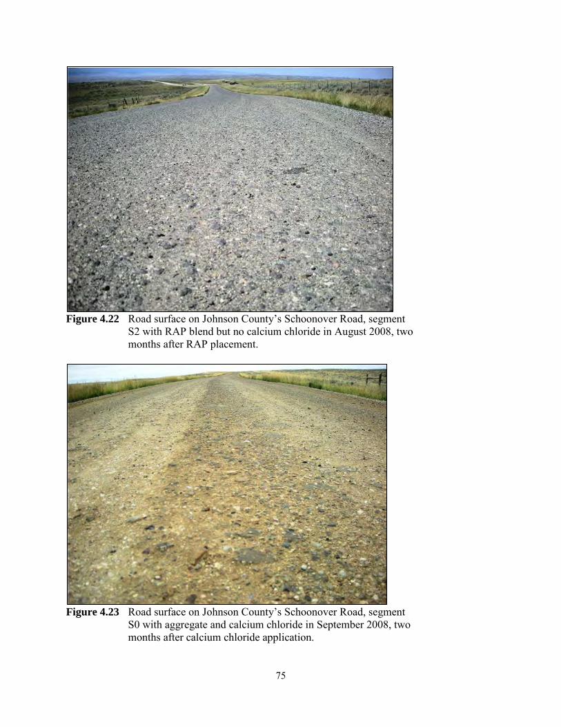
75

Figure 4.22 Road surface on Johnson County’s Schoonover Road, segment

S2 with RAP blend but no calcium chloride in August 2008, two months after RAP placement.

Figure 4.23 Road surface on Johnson County’s Schoonover Road, segment

S0 with aggregate and calcium chloride in September 2008, two months after calcium chloride application.

76

Figure 4.24 Road surface on Johnson County’s Schoonover Road,

segment S1 with RAP and calcium chloride in October 2008, four months after RAP placement and three months after

calcium chloride application.

Figure 4.25 Road surface on Johnson County’s Schoonover Road,

segment S2 with RAP but no calcium chloride in October 2008, four months after RAP placement.

77

4.4.3 Unsurfaced Road Condition Index

Figure 4.26 plots the overall unsurfaced road condition index (URCI) and the deduct values for rutting and loose aggregate as a function of time during the summer and fall of 2008 on the Johnson County test sections. The only distress recorded during the URCI rating other than loose aggregate and rutting was washboards for the gravel and calcium chloride section in October. The overall URCI is controlled almost entirely by loose aggregate and rutting. Loose aggregate ultimately was a minor distress for all three sections, with the loose aggregate taking longer to develop on the sections with calcium chloride. There was more rutting on the sections with calcium chloride and less on the sections with RAP.

Figure 4.26 Unsurfaced road condition indexes and deduct values for ruts

and loose aggregate (LA) on Johnson County’s Schoonover Road for segments S0 with gravel and calcium chloride (G&C), S1 with RAP blend and calcium chloride, and S2 with RAP blend only.


The dustometer measurements are shown in Figure 4.27. Before the application of calcium chloride, the sections with RAP emitted considerably more dust. Once the calcium chloride was applied, the dust from the RAP sections was reduced, though this took place on both the section with and the section without calcium chloride. It took over a month for the section with calcium chloride but without RAP to set up to the point where it wasn’t emitting considerable dust. Several months after application of the calcium chloride, the RAP with calcium chloride gave off more dust than both the aggregate and calcium chloride section and the RAP only section. This surprising result may be because the RAP with calcium chloride section softened up, yielding a

0

10

20

30

40

50

60

70

80

90

100

11-Jul 10-Aug 9-Sep 9-Oct

G&C-URCI RAP-URCI RAP&C-URCIG&C-Ruts G&C-LA RAP-RutsRAP-LA RAP&C-Ruts RAP&C-LA

UR

CI

Deduct V

alues

78

rough, rutted surface that was easily abraded when dry, thus emitting considerable dust; the other sections were smoother so the surface wasn’t ground up as much when it dried, so they emitted less dust.

Figure 4.27 Dust measurements from the dustometer before and

after calcium chloride application on Johnson County’s Schoonover Road for segments S0 with gravel and calcium chloride, S1 with RAP blend and calcium chloride, and S2 with RAP blend only.

4.5 Sweetwater County


Roadway samples were collected in October 2010, about two months after the milled cement-treated base (CTB) and RAP sections were constructed. Figure 4.28 shows the average gradations for the crushed base (CB), CTB, and RAP; Figures 4.29 through 4.31 show the gradations for the CB, CTB, CTB to RAP transition, and RAP sections. All roadway samples were non-plastic.

0.00.20.40.60.81.01.21.41.61.82.0

3-Ju

n

3-Ju

l

2-A

ug

1-Se

p

1-O

ct

S0-G-U/CS1-RAP/G-U/CS2-RAP/G-U

CaCl2 applied tosections S0 and S1

Solid markers indicatethat the section at thistime had been treatedwith calcium chloride.

gram

s/mile

79

Figure 4.28 Average gradations of in-place crushed base (CB), milled

cement-treated base (CTB) blend, and reclaimed asphalt pavement (RAP) blend from Sweetwater County’s Crooks Gap Road, October 2010, two months after construction.

Figure 4.29 Crushed base gradations within WYDOT Grading W specifications as collected from the roadway on section D of Sweetwater County’s Crooks Gap Road, October 2010, two months after construction.

0%

20%

40%

60%

80%

100%

CB CTB RAP

Perc

ent P

assin

g

Sieve#200

⅜"#4 #8 #30 #50 #100½"

¾"1"

0%

20%

40%

60%

80%

100%D MP 1.7D MP 1.8Grading W MinimumGrading W Maximum

Sieve#200

⅜"#4 #8 #30 #50 #100½"

¾"1"

1½"

Perc

ent P

assin

g

80

Figure 4.30 Cement-treated base (CTB) and existing surfacing blended

gradations with the average, minimum and maximum of 9 samples collected from sections E through J of the roadway on Sweetwater County’s Crooks Gap Road, October 2010, two months after construction.

Figure 4.31 Reclaimed asphalt pavement (RAP) and existing surface

blended gradations with the average, minimum and maximum of 6 samples collected from sections L through M on Sweetwater County’s Crooks Gap Road, October 2010, two months after construction.

0%

20%

40%

60%

80%

100%Minimum Average Maximum

#200

Perc

ent P

assin

g

Sieve⅜"#4 #8 #30 #50 #100½"

¾"1"

0%

20%

40%

60%

80%

100%Minimum Average Maximum

Sieve#200

Perc

ent P

assin

g

⅜"#4 #8 #30 #50 #100½"

¾"1"

81


4.5.2.1 Crushed Base Treated with Magnesium Chloride

Sections A and B (see Table 3.3 and Figure 3.8) with crushed base and treated with magnesium chloride were not modified as part of this project; they were monitored as a control section. They generally performed well, forming a good crust and emitting no to minimal dust (see Figure 4.32), though they had roughness resembling very small potholes (see Figure 4.33); these may be caused when very small depressions present when the magnesium chloride brine is placed concentrate the salt in roughly 6-inch diameter pools, forming small-scale roughness as they differentially hold moisture.

Figure 4.32 Road surface made of limestone crushed base treated with magnesium

chloride on Sweetwater County’s Crooks Gap Road.

4.5.2.2 Crushed Base Treated with Lignin Sulfonate and Magnesium Chloride

Sections C and D (see Table 3.3 and Figure 3.8) were surfaced with crushed base and treated with a lignin sulfonate and magnesium chloride blend. Section C is fairly flat, on a long, gentle curve, while section D is a large, downhill s-curve.

Before treatment, these sections were dusty since they had inadequate binder for untreated surfacing gravel. The dust on the uphill and downhill curves of section D (see Figure 4.34) was worse than on the flat curve of section C (see Figure 4.35).

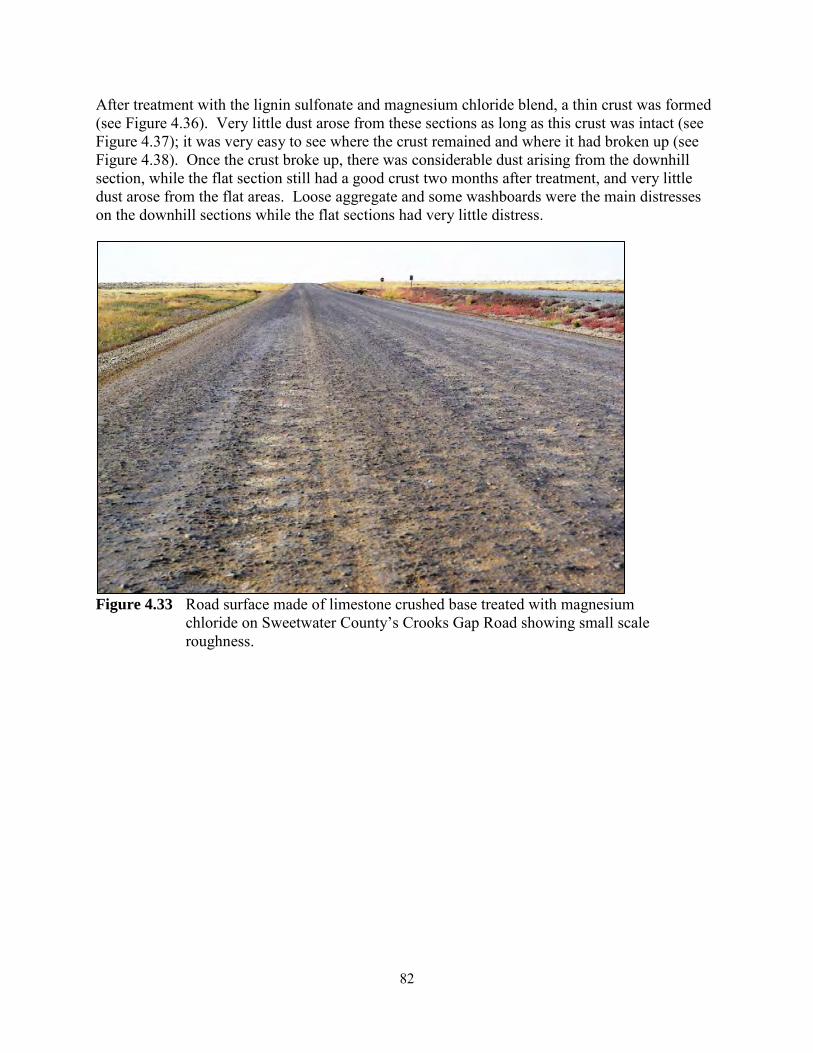
82

After treatment with the lignin sulfonate and magnesium chloride blend, a thin crust was formed (see Figure 4.36). Very little dust arose from these sections as long as this crust was intact (see Figure 4.37); it was very easy to see where the crust remained and where it had broken up (see Figure 4.38). Once the crust broke up, there was considerable dust arising from the downhill section, while the flat section still had a good crust two months after treatment, and very little dust arose from the flat areas. Loose aggregate and some washboards were the main distresses on the downhill sections while the flat sections had very little distress.

Figure 4.33 Road surface made of limestone crushed base treated with magnesium

chloride on Sweetwater County’s Crooks Gap Road showing small scale roughness.

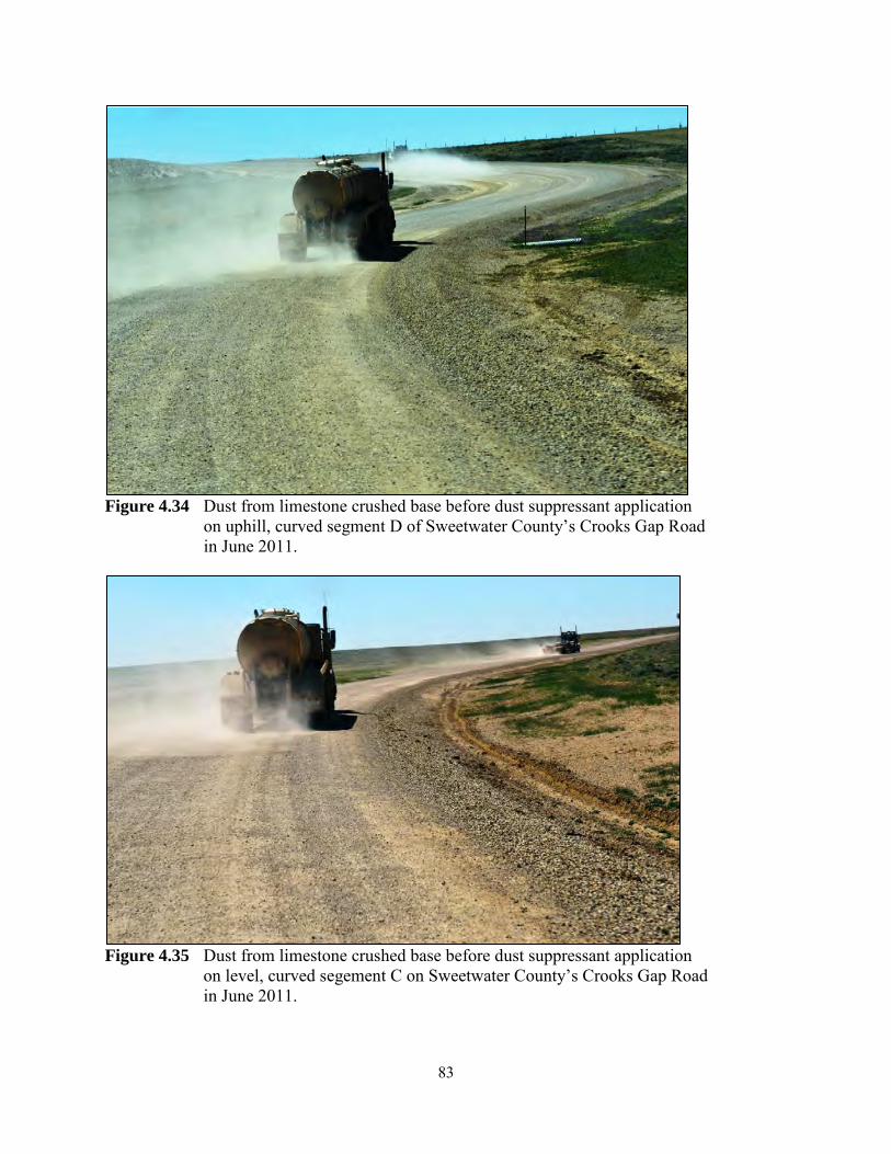
83

Figure 4.34 Dust from limestone crushed base before dust suppressant application

on uphill, curved segment D of Sweetwater County’s Crooks Gap Road in June 2011.

Figure 4.35 Dust from limestone crushed base before dust suppressant application

on level, curved segement C on Sweetwater County’s Crooks Gap Road in June 2011.

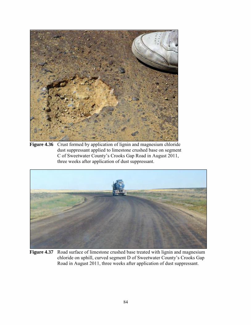
84

Figure 4.36 Crust formed by application of lignin and magnesium chloride

dust suppressant applied to limestone crushed base on segment C of Sweetwater County’s Crooks Gap Road in August 2011, three weeks after application of dust suppressant.

Figure 4.37 Road surface of limestone crushed base treated with lignin and magnesium

chloride on uphill, curved segment D of Sweetwater County’s Crooks Gap Road in August 2011, three weeks after application of dust suppressant.

85

Figure 4.38 Broken up crust of limestone crushed base, foreground, and still intact crust,

background, both treated with lignin and magnesium chloride on uphill, curved segment D of Sweetwater County’s Crooks Gap Road in September 2011, eight weeks after application of dust suppressant.

4.5.2.3 Cement-Treated Base Treated with Polymer and Magnesium Chloride

Sections E through J (see Table 3.3 and Figure 3.9) were all constructed with milled cement-treated base, and all were quite dusty before treatment. During initial construction and the following spring, it was noted that the CTB north of about MP 3.0 (see Figure 4.39) was finer and dustier than that to the south (see figure 4.40), but by the time the road was prepared for treatment with the dust suppression agents there was no visible difference between the CTB sections—both were quite dusty, with considerable loose aggregate and some washboarding.

Shortly after treatment, there was very little dust arising from either the magnesium chloride sections (see Figures 4.41) or the magnesium chloride and polymer blend section (see Figure 4.42). However, as the crust was broken up, the dust became very thick (see Figure 4.43) on all the CTB sections.

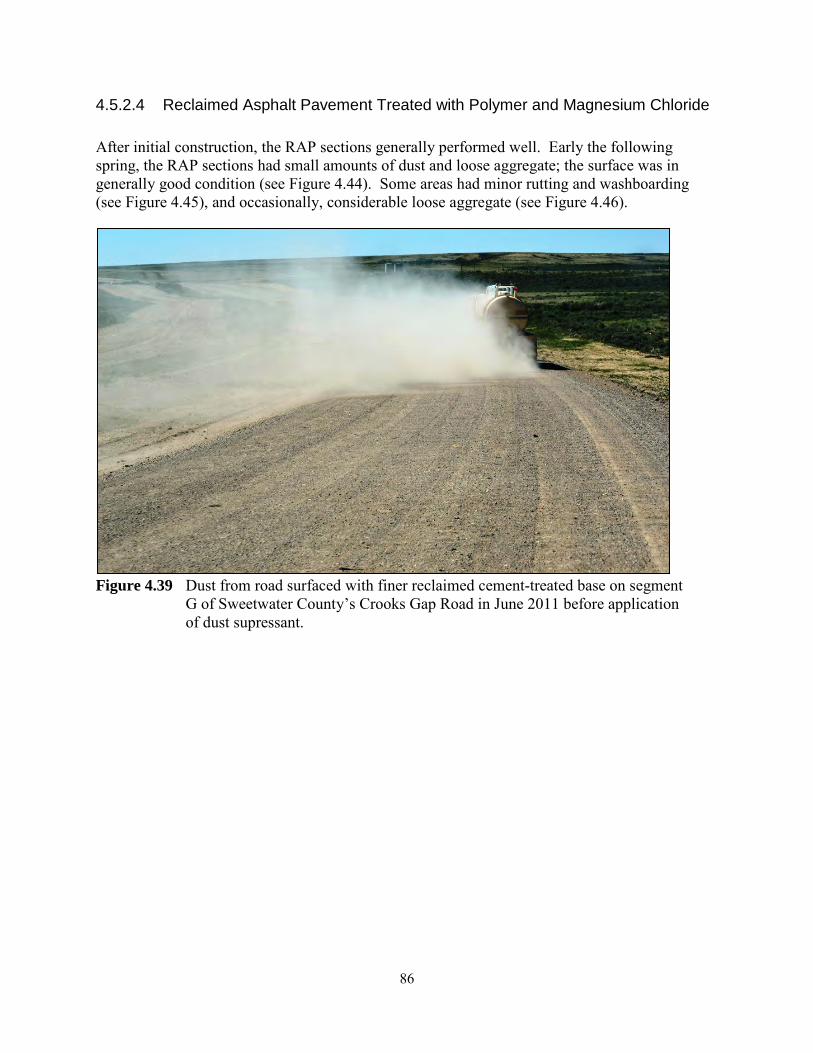
86

4.5.2.4 Reclaimed Asphalt Pavement Treated with Polymer and Magnesium Chloride

After initial construction, the RAP sections generally performed well. Early the following spring, the RAP sections had small amounts of dust and loose aggregate; the surface was in generally good condition (see Figure 4.44). Some areas had minor rutting and washboarding (see Figure 4.45), and occasionally, considerable loose aggregate (see Figure 4.46).

Figure 4.39 Dust from road surfaced with finer reclaimed cement-treated base on segment

G of Sweetwater County’s Crooks Gap Road in June 2011 before application of dust supressant.

87

Figure 4.40 Dust from road surfaced with coarser reclaimed cement-treated base on

segment E of Sweetwater County’s Crooks Gap Road in June 2011 before application of dust suppressants.

Figure 4.41 Road surface with good crust made of reclaimed cement-treated base treated with

magnesium chloride on segment F of Sweetwater County’s Crooks Gap Road in August 2011, three weeks after application of dust suppressant.

88

Figure 4.42 Road surface with good crust made of reclaimed cement-treated base treated with

polymer and magnesium chloride on segment G of Sweetwater County’s Crooks Gap Road in August 2011, three weeks after application of dust suppessant.

Figure 4.43 Dust from road surface made of reclaimed cement-treated base

blended with existing aggregate and treated with magnesium chloride on segment J of Sweetwater County’s Crooks Gap Road in September 2011, eight weeks after application of dust suppressants.

89

Figure 4.44 Road surface made from RAP blended with existing aggregate

on segment M of Sweetwater County’s Crooks Gap Road in March 2011, before the application of dust suppressants.

Figure 4.45 Road surface made from RAP blended with existing aggregate on

segment K of Sweetwater County’s Crooks Gap Road in April 2011, before application of dust suppressant.

90

Figure 4.46 Road surface made from RAP blended with existing aggregate on segment Q of

Sweetwater County’s Crooks Gap Road in April 2011 without dust suppression agents.

A few weeks after treatment, the RAP sections performed well, with little to no dust and generally good surface conditions on the sections treated with magnesium chloride and polymer (see Figure 4.47), those treated with magnesium chloride (see Figure 4.48), and those that were not treated (see Figure 4.49). The untreated sections had very similar surface conditions to the treated sections, though they had noticeably more dust.

Two months after treatment, the magnesium chloride (see Figure 4.50), magnesium chloride with polymer (see Figure 4.51), and untreated RAP sections (see Figure 4.52) were all performing well. The untreated section still exhibited somewhat more dust, though still at acceptable levels.

91

Figure 4.47 Road surface made from RAP blended with existing aggregate treated with

magnesium chloride and polymer on segment M of Sweetwater County’s Crooks Gap Road in August 2011, three weeks after application of dust suppressant.

Figure 4.48 Road surface made from RAP blended with existing aggregate and treated with

magnesium chloride on segment of Sweetwater County’s Crooks Gap Road in August 2011, three weeks after application of dust suppressant.

92

Figure 4.49 Road surface made from RAP blended with existing aggregate on

segment P of Sweetwater County’s Crooks Gap Road in August 2011.

Figure 4.50 Road surface made with RAP blended with existing aggregate and treated

with magnesium chloride on segment N of Sweetwater County’s Crooks Gap Road in September 2011, eight weeks after application of dust suppressant.

93

Figure 4.51 Road surface made with RAP blended with existing aggregate and treated

with magnesium chloride and polymer on segment L of Sweetwater County’s Crooks Gap Road in September 2011, eight weeks after application of dust suppressant.

Figure 4.52 Road surface made with RAP blended with existing aggregate on segment P of

Sweetwater County’s Crooks Gap Road in September 2011.

94

4.5.3 Unsurfaced Road Condition Index

The Sweetwater County test sections’ unsurfaced road condition indexes (URCI) were measured for each of the fifteen sections listed in Table 3.3. The URCI was assessed four times: Once during spring on April 27; once in the summer just before the dust suppressants were applied on July 7; three weeks after the dust suppressants were applied on August 10; and again seven weeks after application on September 8. The URCIs for sections receiving the same treatment were averaged and plotted in Figure 4.53. All treated sections showed higher, improved URCIs; the crushed base sections that had already been treated remained in the same condition; and the untreated RAP sections’ URCI declined.

Figure 4.53 Average unsurfaced road condition indexes (URCI) for test segments on

Sweetwater County’s Crooks Gap Road in 2011.

In the following sections, the deduct values for four of the five observed and measured distresses are discussed. (Dust was also visually assessed as part of determining the URCI, but dust emissions are discussed in section 4.5.3 below using the quantitative dustometer measurements—four subjective levels of dust are used to calculate the URCI: None, Low, Medium, and High. See section 4.1 above for a more detailed discussion of these two types of road dust assessment.) The other two distresses used to compile an URCI, “cross section” and “roadside drainage,” were not at a level where any deduction was made on their account since all the roads in these studies are well drained and shaped.

60

70

80

90

100

CB & MgCl2 CB/CB & MgCl2-LigninCTB/CTB & MgCl2 CTB/CTB & MgCl2-PolymerRAP/RAP & MgCl2 RAP/RAP & MgCl2-PolymerRAP

UR

CI

April 27 July 7 Aug 10

July 19-21: Dustsuppressants applied

Open markers: UntreatedFilled markers: Treated

Sept 8

Maintenance: August 16 & 29

95

The distresses described in sections 4.5.3.1 through 4.5.3.4 below are presented in order, with the distress causing the greatest deducts, loose aggregate, first and the one causing the fewest deducts, potholes, listed last. In all cases, higher deduct values mean poorer performance and more distress on the roadway surface. The URCI system is set up so that a given number of deduct points indicates the same degree of distress, regardless of which type of distress one is assessing. Therefore, one can compare the severity of, for example, loose aggregate versus rutting, by looking at the deduct values for each, concluding that the distress with the highest deduct value makes the greatest negative contribution to the quality of the roadway surface, loose aggregate in this case. In short, high deduct values indicate poor performance, and they are listed first in the following four sections.

4.5.3.1 Loose Aggregate

Figure 4.54 plots the loose aggregate values before and after the dust suppressants were applied. For the RAP and gravel sections, loose aggregate was virtually eliminated once they formed a good crust and set up, but the CTB sections after an initial reduction in loose aggregate returned to their previous condition of considerable loose aggregate. The dust suppressants provided only a brief respite from the loose aggregate, as is also demonstrated below for washboards and dust.

Figure 4.54 Average loose aggregate deduct values for test segments on Sweetwater

County’s Crooks Gap Road in 2011.

0

5

10

15

20

25


Loos

e A

ggre

gate

Ded

uct V

alue

s




Sept 8


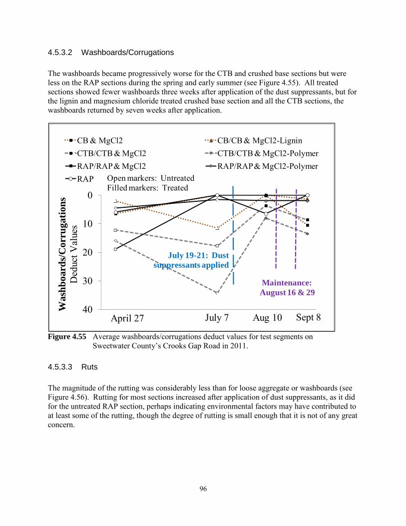
96

4.5.3.2 Washboards/Corrugations

The washboards became progressively worse for the CTB and crushed base sections but were less on the RAP sections during the spring and early summer (see Figure 4.55). All treated sections showed fewer washboards three weeks after application of the dust suppressants, but for the lignin and magnesium chloride treated crushed base section and all the CTB sections, the washboards returned by seven weeks after application.

Figure 4.55 Average washboards/corrugations deduct values for test segments on

Sweetwater County’s Crooks Gap Road in 2011.

4.5.3.3 Ruts

The magnitude of the rutting was considerably less than for loose aggregate or washboards (see Figure 4.56). Rutting for most sections increased after application of dust suppressants, as it did for the untreated RAP section, perhaps indicating environmental factors may have contributed to at least some of the rutting, though the degree of rutting is small enough that it is not of any great concern.

0

10

20

30

40


Was

hboa

rds/C

orru

gatio

nsD

educ

t Val

ues




Sept 8


97

4.5.3.4 Potholes

Like rutting, potholes are not a major distress on any of the sections (see Figure 4.57). Potholes were reduced initially with the application of dust suppressants, but returned by seven weeks after application-like rutting as described in the previous section.

Figure 4.56 Average ruts deduct values for test segments on Sweetwater County’s

Crooks Gap Road in 2011.

0

2

4

6

8

10

12

14


Rut

sD

educ

t Val

ues




Sept 8


98

Figure 4.57 Average potholes deduct values for test segments on Sweetwater

County’s Crooks Gap Road in 2011.


Figure 4.58 shows the grams per mile of dust collected with the dustometer. The scale is quite large since on the final measurement upwards of 3 grams per mile were collected. This is probably due to a combination of recent maintenance made necessary by excessive washboards, and of the inability of the CTB to maintain a crust that resists dust and abrasion.

0

1

2

3

4

5


Poth

oles

Ded

uct V

alue

s




Sept 8


99

Figure 4.58 Average dust measured with the dustometer on test segments on

Sweetwater County’s Crooks Gap Road in 2011, full scale.

Figure 4.59 is on a smaller scale, with all plotted values within the medium to low dust range—less than 1.0 grams per mile as described in section 4.1 above. As one would expect, the dust values are generally lower for all treated sections three weeks after application, though at seven and eight weeks after application most sections’ dust has begun to increase, though only the CTB sections showed dramatic increases with values in the “High” dust range, a hazardous condition. Much of this increase is probably due to environmental factors since the untreated RAP section also had substantially more dust eight weeks after application.

0

1

2

3

4


Dus

t gr

ams/m

ile


August 10

July 19-21:Dust

suppressantsapplied

July 8 Sept 8 Sept 15


100

Figure 4.59 Average dust measured with the dustometer on test segments on Sweetwater

County’s Crooks Gap Road in 2011, partial scale.

4.6 Summary of Results

This chapter describes the dust evaluation techniques used in this study. It also describes the results obtained from the test sections in the three counties.

This chapter begins by describing the analyses that suggest correlations between the subjective dust ratings from the USACE’s URCI rating system (Eaton and Beaucham 1992) and the CSU dustometer readings (Sanders and Addo 2000) Cutoffs of 0.15, 0.40 and 1.00 grams per mile are suggested to differentiate between None, Low, Medium and High subjective dust ratings using the URCI system.

Next, environmental influences on the values obtained with the dustometer are evaluated, yielding several recommendations for the use of the dustometer. Surfacing age is assessed: when interpreting the results from the dustometer, one should consider the time since the road was last treated, maintained, or constructed. Moisture content is assessed: measurements should not be conducted when the surface is noticeably damp or when recent precipitation is apparently preventing dust emissions. Wind speed is assessed: measurements should be taken when wind is as light as possible, and measurements should not be taken when wind speeds are greater than 15 mph. When these parameters are followed, the dustometer provides reasonable, easily collected results that reflect fugitive dust emissions from the roadway.

0.0

0.2

0.4

0.6

0.8

1.0


Dus

t gr

ams/m

ile


August 10July 8 Sept 8 Sept 15

July 19-21:Dustsuppressantsapplied


101

The Laramie County sections had considerable distresses related to segregation caused by the inability of the motor grader to compensate for the longitudinally inconsistent placement of RAP from haul trucks. Loose aggregate was the most significant distress on the test sections. Before a good crust formed, there was also considerable fugitive dust emission.

The Johnson County test sections performed well, largely due to the excellent uniformity of the RAP and virgin aggregate blend achieved with a pugmill at the stockpile. Interestingly, the section with RAP but without any calcium chloride dust suppressant performed best, even in terms of fugitive dust emissions. The RAP section with calcium chloride exhibited more rutting and surface roughness; this roughness may have led to more abrasion and raveling that, in turn, led to more dust.

The Sweetwater County sections results are more complex since they involved more test sections than the other two counties combined. The CTB sections all exhibited considerable fugitive dust, loose aggregate, and washboards, except for a month to six weeks after application of magnesium chloride-based dust suppressants when a good crust formed and prevented these distresses. The crushed base sections on the flat performed well with either straight magnesium chloride or with a magnesium chloride and lignin sulfonate blend. However, the lignin blend exhibited considerable washboards, loose aggregate, and dust on the long hill within six weeks of treatment. The RAP sections all performed well. They developed a good crust after some initial loose aggregate on the sections with the polymer blend and those without any dust suppressant. By seven weeks after treatment, the loose aggregate had set up adequately on all the RAP sections. Those treated with magnesium chloride or with a magnesium chloride and polymer blend had somewhat more rutting and potholes, while the section without any dust suppressant had more dust. However, all these distresses on the RAP sections were relatively minor. Overall, the crushed base performed well with magnesium chloride and on the flat, but it did not perform well on the hill. The RAP performed well but the CTB did not.

103

5. ECONOMIC ANALYSES

In order to fulfill one of the objectives of this study, the research team utilized cost information from an I-80 project where WYDOT utilized RAP in the base and asphalt surface layer. In addition, WYDOT provided Sweetwater County with RAP so that it could be incorporated in a gravel road with very heavy truck traffic. The cost and benefits obtained at this location were used to develop the methodology to determine which application is more cost effective.

5.1 Study Section: Sweetwater County Road 23: Crooks Gap Road

The gravel test sections were constructed on County Road 23 (SWCR 23) in Sweetwater County, just north of Wamsutter, Wyoming. The entire section spanned eight miles, and was broken down into smaller individual test sections. The data from these test sections will be used concurrently with data from a WYDOT project on Interstate 80, IM-0803135. The I-80 data will be used for the cost analysis of RAP in Hot Plant Mix and RAP in base.

There were two half-mile sections constructed using RAP. The RAP was distributed using bottom discharge dump trucks and then spread with a motor grader. The RAP and base were then mixed by a CAT RM-500 Rotary Mixer as shown in Figure 3.30. This machine mixed the RAP with six inches of base and released the mixture back onto the road surface. The RAP mixture was then sprayed with water and compacted to achieve maximum density.

5.2 Cost-Benefit Analysis Method

The cost benefit analysis method that was used is described in the appendix of Informational Series 123 by the National Asphalt Pavement Association. The exact method was used for the RAP in Hot Plant Mix (RHPM) but there were some modifications made for RAP in base and for RAP used in gravel roads. The procedure for this analysis is described in section 5.5 below and the modifications are shown in the individual applications within the case study, section 5.6 below.

The economic comparison was developed by analyzing the price per ton of applied RAP for three different application types. First, the difference between RAP in RHPM and Virgin Hot Plant Mix (HPM) was evaluated. The individual prices for materials and the amount of each material in the mixture was taken into consideration. Second, the economic difference between RAP in road base and virgin road base was studied. Finally, the economic benefit was calculated for RAP in gravel roads. These analyses include savings factors such as dust reduction, layer coefficients, haul cost, and savings from virgin aggregate.

5.3 Data Collection

The data collection began by acquiring prices and amounts of materials required in each of three RAP applications. The 2010 WYDOT Average Bid prices, as well as the Materials and Rates Summary from Project IM-0803135, were obtained for both RHPM and RAP in road base

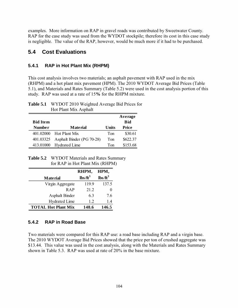
104

examples. More information on RAP in gravel roads was contributed by Sweetwater County. RAP for the case study was used from the WYDOT stockpile; therefore its cost in this case study is negligible. The value of the RAP, however, would be much more if it had to be purchased.

5.4 Cost Evaluations

5.4.1 RAP in Hot Plant Mix (RHPM)

This cost analysis involves two materials; an asphalt pavement with RAP used in the mix (RHPM) and a hot plant mix pavement (HPM). The 2010 WYDOT Average Bid Prices (Table 5.1), and Materials and Rates Summary (Table 5.2) were used in the cost analysis portion of this study. RAP was used at a rate of 15% for the RHPM mixture.

Table 5.1 WYDOT 2010 Weighted Average Bid Prices for Hot Plant Mix Asphalt

Table 5.2 WYDOT Materials and Rates Summary for RAP in Hot Plant Mix (RHPM)

5.4.2 RAP in Road Base

Two materials were compared for this RAP use: a road base including RAP and a virgin base. The 2010 WYDOT Average Bid Prices showed that the price per ton of crushed aggregate was $13.44. This value was used in the cost analysis, along with the Materials and Rates Summary shown in Table 5.3. RAP was used at rate of 20% in the base mixture.

Bid Item Number Material Units

Average Bid

Price401.02000 Hot Plant Mix Ton $30.61401.03325 Asphalt Binder (PG 70-28) Ton $622.37413.01000 Hydrated Lime Ton $153.68

MaterialRHPM, lbs/ft3

HPM, lbs/ft3

Virgin Aggregate 119.9 137.5RAP 21.2 0

Asphalt Binder 6.3 7.6Hydrated Lime 1.2 1.4

TOTAL Hot Plant Mix 148.6 146.5

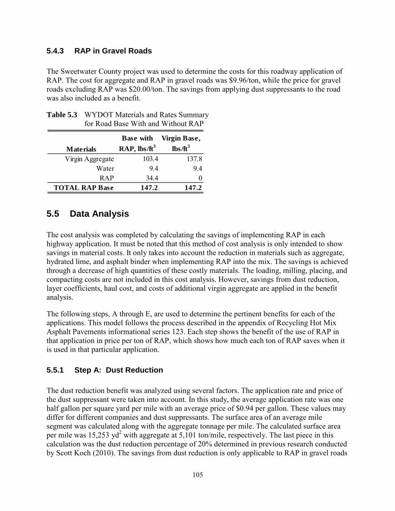
105

5.4.3 RAP in Gravel Roads

The Sweetwater County project was used to determine the costs for this roadway application of RAP. The cost for aggregate and RAP in gravel roads was $9.96/ton, while the price for gravel roads excluding RAP was $20.00/ton. The savings from applying dust suppressants to the road was also included as a benefit.

Table 5.3 WYDOT Materials and Rates Summary for Road Base With and Without RAP

5.5 Data Analysis

The cost analysis was completed by calculating the savings of implementing RAP in each highway application. It must be noted that this method of cost analysis is only intended to show savings in material costs. It only takes into account the reduction in materials such as aggregate, hydrated lime, and asphalt binder when implementing RAP into the mix. The savings is achieved through a decrease of high quantities of these costly materials. The loading, milling, placing, and compacting costs are not included in this cost analysis. However, savings from dust reduction, layer coefficients, haul cost, and costs of additional virgin aggregate are applied in the benefit analysis.

The following steps, A through E, are used to determine the pertinent benefits for each of the applications. This model follows the process described in the appendix of Recycling Hot Mix Asphalt Pavements informational series 123. Each step shows the benefit of the use of RAP in that application in price per ton of RAP, which shows how much each ton of RAP saves when it is used in that particular application.

5.5.1 Step A: Dust Reduction

The dust reduction benefit was analyzed using several factors. The application rate and price of the dust suppressant were taken into account. In this study, the average application rate was one half gallon per square yard per mile with an average price of $0.94 per gallon. These values may differ for different companies and dust suppressants. The surface area of an average mile segment was calculated along with the aggregate tonnage per mile. The calculated surface area per mile was 15,253 yd2 with aggregate at 5,101 ton/mile, respectively. The last piece in this calculation was the dust reduction percentage of 20% determined in previous research conducted by Scott Koch (2010). The savings from dust reduction is only applicable to RAP in gravel roads

MaterialsBase with

RAP, lbs/ft3Virgin Base,

lbs/ft3

Virgin Aggregate 103.4 137.8Water 9.4 9.4RAP 34.4 0

TOTAL RAP Base 147.2 147.2

106

because road base with RAP and RHPM do not produce dust. Equation 1 can be used to calculate the benefit from dust reduction.

(Surface Area [yd2])*(Application Rate [gal/yd2/mile])*(Price [$/ga]) (Total Aggregate [ton/mile])*(Dust Reduction [%])

5.5.2 Step B: Layer Coefficients

The layer coefficient benefit became negligible because WYDOT specifications dictate that blended and crushed base have equal layer coefficients of 0.12. Other agencies may use this same calculation for determining a layer coefficient benefit when blended and crushed base have different coefficients. When calculating the savings, the crushed base was divided by the blended base coefficient. Equation 2 is used to determine the monetary benefit due to layer coefficients.

(Blended Base Layer Coefficient)*(Price Virgin Aggregate [$/ton])

5.5.3 Step C: Haul Costs

The haul costs were an important factor because additional cost is incurred to haul aggregate to the site of application. Considering the RAP in this case study was stockpiled on site, the haul distance was negligible and therefore had no effect on costs. Haul costs could still have an impact in other projects, so a method for evaluating haul is shown below. The haul cost would be affected depending on the percent of RAP in the mix. A higher percentage of RAP in the mix design would require more material and thus more haul. Equation 3 was used to find the addition costs from haul. The hauling costs should be subtracted from the total benefit.

(Distance [miles])*(Haul Rate [$/ton/mile])

5.5.4 Step D: Savings from Virgin Aggregate

This savings comes from the difference in cost by using RAP in the mix rather than additional virgin aggregate from outside sources. The utilization of RAP will lead to a lower cost in the new road application. This value will differ for the RHPM, RAP in gravel roads and RAP in road base. The savings from the decreased used of virgin aggregate can be determined using Equation 4.

(Virgin Aggregate [$/ton]) – (Blended Aggregate [$/ton])

5.5.5 Step E: Total Benefit

The total benefit of using RAP in an application is calculated using the four steps listed (A-D). Table 5.4 outlines the process for determining the net benefit from each of the factors considered. Steps A through D are completed and the final step E is used to sum the benefits and costs to determine which application of RAP is the most ideal.

(1)

(2)

(3)

(4) (4)

107

5.6 Case Study

A case study was conducted to test this cost/benefit approach and illustrate how it could be applied in many situations. This case study utilized the three Wyoming RAP applications: RAP in hot plant mix, RAP in base, and RAP used on gravel roads. The following section shows how each highway application is evaluated and illustrates the benefit analysis process.

Table 5.4 Benefit Analysis Template Using All Factors

5.6.1 RAP in Hot Plant Mix (RHPM)

To calculate the cost difference by using RAP in Hot Plant Mix, the price for each component of the total material must be calculated. This is done by taking the amount of that individual material and multiplying it by its inverse unit weight to obtain an amount. Then, this amount is multiplied by the price per ton to finally reach a figure for that respective component. This process is shown in Table 5.5.

Step FactorsRoad

ApplicationSavings from Dust Reduction:(Surface Area [yd 2 ])*(Application Rate [gal/yd 2 /mile])*(Price [$/gal])

(Total Aggregate [ton/mile])*(Percent Dust Reduction)Savings from Layer Coefficients:

(Blended Base Layer Coefficient)*(Price Virgin Aggregate [$/ton])(Crushed Base Layer Coefficient)

Negative Savings from Haul:(Distance [miles])*(Haul Rate [$/ton/mile])

Savings from Virgin Aggregate:(Virgin Aggregate [$/ton]) - (Blended Aggregate [$/ton])

E Total Benefit (A + B + C + D) $/ton RAP

A$/ton RAP

$/ton RAP

$/ton RAP

$/ton RAP

B

C

D

108

Table 5.5 RHPM Material Calculations

Table 5.6 illustrates the savings incurred when using RHPM over HPM. The calculations were converted to price per ton of RAP to provide for a comparison mechanism of cost savings for all three construction techniques. This was accomplished by incorporating the percent of RAP in the mixture with the savings. Therefore,

$6.13 𝑝𝑒𝑟 𝑡𝑜𝑛 𝐻𝑀𝐴0.15

= $40.87

yields the savings per ton of RAP.

Table 5.6 Cost Saving by Using RHPM Instead of HPM

It can be observed from the calculations in Table 5.7 that a substantial savings is accomplished by using RAP in the asphalt mixture. A savings of $40.87 per ton of RAP was saved by implementing a 15% RAP mix, meaning the value of RAP in HMA is $40.87/ton. This savings would increase by using a greater amount of RAP in the HPM.

RHPM HPM

Unit Weight, lb/ft3 148.61 146.50Asphalt Binder

lb/ft3 6.3 7.6$/ton $622.37 $622.37Cost $26.39 $32.29

Hydrated Limelb/ft3 1.2 1.4$/ton $153.68 $153.68Cost $1.24 $1.47

Hot Plant Mixlb/ft3 148.6 146.5$/ton $30.61 $30.61Cost $30.61 $30.61

TOTAL $58.24 $64.37

MaterialRHPM,

$/tonHPM, $/ton

Savings, $/ton

Asphalt Binder $26.39 $32.29 $5.90Hydrated Lime $1.24 $1.47 $0.23

Total Hot Plant Mix $30.61 $30.61 $0.00TOTAL $58.24 $64.37 $6.13

109

Table 5.7 Cost Savings from Using RHPM Instead of HPM

5.6.2 Road Base with RAP

This analysis was completed using the same method as the RHPM cost/benefit analysis. The amount of each component was converted into a ratio by multiplying its amount by the inverse unit weight. Then, the value was multiplied by the price per ton to reach a price figure. For the case study, the only component being calculated was the aggregate because RAP and water were supplied by WYDOT. Tables 5.8 and 5.9 show the calculations and steps to determine the savings associated with using RAP in base.

Table 5.8 Cost of Road Base With and Without RAP

Table 5.9 Cost-Benefit Analysis for RAP in Road Base

Table 5.9 shows how the price for the RAP base is $15.71 per ton of RAP less than the price for base without RAP. This savings is largely because less virgin aggregates were needed. The blended RAP base is cheaper, proving that the addition of RAP to highway applications is economically feasible.

Step Factor RHPMA Savings from Dust Reduction N/AB Savings from Layer Coefficients N/AC Negative Savings from Haul N/AD Savings from Virgin Aggregate $40.87E Total Benefit (A + B + C + D) $40.87

Base with RAP

Virgin Base

Unit Weight, lb/ft3 103.4 137.8Aggregate, lb/ft3 13.44 13.44

Conversion to ton, RAP 20% 5 5Costs, %/ton RAP $47.20 $62.91

Step FactorsRAP in Base

A Savings from Dust Reduction N/AB Savings from Layer Coefficients N/AC Negative Savings from Haul N/AD Savings from Virgin Aggregate $15.71E Total Benefit (A + B + C + D) $15.71

110

5.6.3 RAP in Gravel Roads

This analysis compared gravel roads with and without RAP. The typical savings from using RAP in the material was found using the two prices provided by Sweetwater County. This savings was $10.04/ton of RAP. This was obtained by finding the difference between, $9.96/ton of RAP for gravel roads and $20.00/ton for gravel roads without RAP. This savings would be included under the factor “Savings from Virgin Aggregate.”

The other factor applied to this analysis was the savings from dust reduction. RAP in gravel roads was the only highway application affected by this factor because it is essentially the only one that releases dust to the environment. The savings was found by using equation 1 under the Dust Reduction method explained earlier. This savings was $7.03/ton of RAP. The cost/benefit analysis is summarized in Table 5.10.

Table 5.10 Cost-Benefit Analysis for RAP in Gravel Roads

This analysis shows that the use of RAP in a highway application saves money. RAP in gravel roads resulted in a saving $17.07/ton of RAP in this case. This was due to the savings from virgin aggregate and the savings through dust reduction, which will keep the road in better condition by retaining the fine particles embedded in the road. The air quality will also be improved as a result of the reduction in dust.

5.7 Summary of Economic Analysis of RAP Use

RAP can be a very effective material in highway construction applications. It is economically feasible to use RAP because the recycled material greatly reduces the need for virgin aggregates. Other studies have shown that, while being cost effective, RAP does not decrease pavement performance. Surface distresses will not occur because of the use of RAP. The addition of RAP significantly reduces the dust loss on gravel roads from traveling vehicles.

Step Factors

RAP in Gravel Roads

A Savings from Dust Reduction $7.03B Savings from Layer Coefficients N/AC Negative Savings from Haul N/AD Savings from Virgin Aggregate $10.04E Total Benefit (A + B + C + D) $17.07

111

Based on the cost analysis described in this paper, when RAP was included in Hot Plant Mix, it offered the greatest amount of savings in any road application studied. For every ton of RAP included in the mixture, $40.87 was saved. There was also savings of $17.07 for every ton of RAP used in gravel roads. The implementation of RAP in road base also saved money, but it was the least effective of the three applications. For every ton of RAP used in road base, $15.71 was saved. This analysis shows that regardless of the construction use of RAP, a savings is always realized.

Clearly, the application of RAP in highway construction is cost effective. The amount of savings can increase exponentially when large quantities are used and when a greater percentage of RAP is included. The use of RAP in asphalt mix is the most cost effective in this case study. Depending on other factors, such as haul or layer coefficients, a different application method could be more beneficial in other situations. The use of RAP in any situation has no shortfalls; RAP saves money, does not impact performance, and has the ability to help the environment due to dust loss in gravel roads.

This approach to determining which application of RAP is most cost effective and beneficial to the area and the sustainability of the roadway is very advantageous. It allows several factors to be assessed and provides for a common comparison among the different uses of RAP. Normalizing the benefit to the savings per ton of RAP allows quick and useful comparisons to be made by not only highway officials but local agencies and the public.

113

6. SUMMARY AND CONCLUSIONS

6.1 Laramie County Performance Summary

The Laramie County construction process did not achieve adequate blending, leading to segregation. This lack of material uniformity led to considerable loose aggregate and a generally poor-performing roadway with excessive loose aggregate, mostly unconsolidated asphalt millings. Additional blending attempted to remove the segregation with some degree of success, though segregation and corresponding variations in performance continued.

Good crust and thus good performance was achieved when the existing aggregate and RAP were well blended. Problems on the Laramie County sections were related to segregation caused by the construction method, not to the materials themselves. Once the crust was formed, dust was at low levels and the surface was reasonably durable.

6.2 Johnson County Performance Summary

The Johnson County test sections generally performed well. Excellent uniformity was achieved by blending the virgin aggregate with the RAP in a pugmill at the stockpile

The section with RAP and calcium chloride did not perform as well as the RAP only section. This was apparently due to softening of the RAP and chloride section leading to roughness, potholes, and, surprisingly, greater dust emissions. This may be due to the extra roughness caused by the softer surface; this may have caused more abrasion as vehicle tires bounced along, kicking up more dust. Still, the RAP and chloride section rutted much less than the aggregate only section with chloride, but the RAP and chloride section emitted the most dust.

Overall, the RAP only section performed best. Undesirable softening due to the chlorides caused the RAP and chloride section to perform worse than the RAP alone.

6.3 Sweetwater County Performance Summary

Generally, good blending was achieved using a reclaimer to mix the CTB or RAP with the underlying material. It is unclear to what degree this was due to the reclaimer itself, and the degree to which the uniformity was due to achieving a good spread from the bottom-discharge haul trucks. It seems probable that both elements played a role. The motor grader and reclaimer achieved substantially better blending than was achieved in Laramie County with motor graders alone. This improvement resulted in only minor segregation and in substantially better performance.

The control section built with WYDOT Grading W limestone crushed base treated with magnesium chloride brine performed well throughout the duration of this study, though some roughness was present. Dust was minimal.

114

The crushed base with lignin sulfonate and magnesium chloride performed well on the flat section but it did not perform well on the hill section. Washboards and dust on the hill section became so severe that they became a safety hazard, necessitating maintenance to reduce the washboards, though the severe dust could not be reduced.

The cement-treated base (CTB) sections did not perform well. They formed a good crust only briefly after application of the magnesium chloride, with or without polymers. Soon they developed excessive washboards that necessitated maintenance, which made the dust even worse. Milled CTB should not be used as an additive to unpaved roads’ surfacing material. It is a major source of dust without any binder to hold the dust in place.

The sections constructed with RAP all performed well. Overall roughness was minor on all the RAP sections. Problems with loose aggregate and washboarding generally diminished with time as a good crust formed, regardless of the presence of chlorides. Rutting and potholes were worse on the sections treated with magnesium chloride, though they were not severe. Dust was worse on the untreated sections, though it was not severe. Good blending introduced some binding material from the existing, underlying surfacing material.This appears to have helped the RAP sections form a good tight crust, avoiding the potentially severe impacts of loose aggregate and washboarding if inadequate binding takes place. It also appears that, with time, the RAP set up more and more, forming a good crust. Perhaps, it would have done so even without the blending with the existing material, though this might have introduced problems if the road surface came up in chunks with the motor grader during routine maintenance, making good, long-term performance difficult.

6.4 Performance as a Function of Construction Methods

It is apparent from this study that getting a consistent blend is critical to good performance of a road with RAP added to its surface. The methods employed in Johnson and Sweetwater Counties were successful in achieving this, but the method used in Laramie County was less successful, resulting in segregation that severely and negatively impacted the performance of those test sections. Using methods that assure good, uniform blending with minimal to no segregation is crucial to good performance.

Blending with a pugmill at the stockpile, as was done in Johnson County, appeared to provide the best, most uniform road surface. However, blending materials placed with bottom-discharge haul trucks with a motor grader and reclaimer, as was done in Sweetwater County, also produced good results, though there was some minor but noticeable segregation with this method. It is unclear whether this minor segregation stemmed from truck-to-truck segregation caused by not stringing out the windrows far enough, or whether it was due to inadequate blending at the original RAP stockpile, or to inadequate blending by the motor grader and reclaimer. In any case, good blending was achieved on the Sweetwater County sections, though generally not as good as on the Johnson County sections.

115

6.5 Performance as a Function of Surfacing Materials

RAP, when well blended with aggregate or existing materials that provide additional binder, makes an excellent unpaved road surface. Blends in the neighborhood of three-quarters RAP and one-quarter aggregate down to half RAP and half virgin aggregate provided a good surface that bound together, though sometimes there was a period of several weeks to several months before the surface set up and loose aggregate diminished as a serious surface defect, particularly for the higher RAP proportion blends.

Two elements are most critical to the performance of RAP as a surfacing aggregate:

• Adequate binder so the RAP blend sets up and forms a good crust. o Otherwise, loose aggregate, washboards, and dust may be serious problems. o Depending on the properties of the fines in the aggregate blended with the RAP,

as little as 20% virgin aggregate may be blended with the RAP. For aggregate with less binding capacity—lower PI and lower percentages passing the #200 [0.075 μm] sieve—as much as 50% aggregate may be closer to optimal.

• Enough virgin aggregate so that the RAP does not set up in chunks which cannot be reworked with a motor grader to reshape the road as distresses appear and crown is lost.

o Thorough blending is essential to achieve this, since otherwise “fat spots” of RAP may be prone to setting up in chunks, especially under heavy traffic in hot weather.

When a proper balance of binding capacity from the virgin aggregate and strength from the RAP is achieved along with uniform mixing to prevent segregation, the use of RAP and aggregate blends as a surfacing material yields a road that performs well, at least in the short term.

Milled cement-treated base (CTB) performed very poorly as an unpaved road surfacing additive. It has too much non-plastic fine material. Though it was mixed with underlying, plastic material on the Sweetwater County test site, the CTB was unable to maintain a crust for much more than a month even with the application of magnesium chloride, albeit under heavy truck traffic. Severe washboards and dust necessitated additional maintenance which broke up the crust, leading to very high dust emissions.

6.6 Performance as a Function of Dust Suppressants

Generally, the chloride dust suppressants—magnesium chloride brine, magnesium chloride brine with a proprietary polymer, and calcium chloride flakes—functioned as one would expect. They held additional moisture in the RAP blends, making it softer, and they reduced fugitive dust emissions.

On the Johnson County test sections, the RAP blend treated with calcium chloride emitted more dust than the RAP section without any calcium chloride. This may have happened because the RAP blend with calcium chloride was softer and more prone to rutting and other surface deformations; this may have led to more bouncing of passing vehicles, leading to greater

116

abrasion, leading to more loose particles and greater grinding of the road surface by tires, thereby causing more dust.

There seems to be little difference in the performance of three of the four chloride types used—calcium chloride flakes, magnesium chloride brine, and magnesium chloride brine with polymers —though the circumstances under which these three chlorides were used were quite different, particularly for the calcium chloride. The calcium chloride was placed on material that was blended at the stockpile and it was placed on entirely different materials.

Similarly, though to a lesser degree, the magnesium chloride and the magnesium chloride with polymer were used somewhat differently—the straight magnesium chloride was applied at 0.50 gallons per yard, while the 50%/50% magnesium chloride and proprietary polymer blend was applied at 0.30 or 0.40 gallons per yard. For reasons relating to excessive softening of the RAP blends due to the addition of chloride dust suppressants, these lower chloride application levels with the polymer blend may have been a good thing. The sections with the polymers and lower total magnesium chloride levels had somewhat more dust but less rutting, though neither distress was severe in any case.

The magnesium chloride and lignin sulfonate blend placed on the crushed base in Sweetwater County formed a thin crust, roughly ⅛ inch thick, that kept down dust while it lasted. However, on the hilly section, the crust quickly broke up, forming washboards and emitting a lot of dust.

Neither the magnesium chloride nor the magnesium chloride and polymer blend was able to hold the CTB together for more than a month, after which it became very dusty. Though there may be treatments that would be successful for CTB used as a surfacing material, these two treatments were not successful in this application.

Overall, the addition of dust suppressants on roads surfaced with a RAP blend seems unnecessary, at least with the RAP and virgin aggregate blends examined in this study. While in some cases, dust was reduced, in others, dust was increased as surface roughness became worse, apparently causing the crust to be broken up by traffic, thereby releasing more fugitive dust. The benefit from treating a RAP and aggregate blend with dust suppressant, at least the hygroscopic chlorides, may be entirely outweighed by the damage that occurs due to the softening of the road surface as more moisture is retained. The RAP blends alone do not emit a lot of dust, so there is relatively little advantage to further reducing their fugitive dust emissions.

6.7 Economics of RAP Use

The highest economic value of reclaimed asphalt pavement, at least in conventional highway applications, is as an additive to hot plant mix pavement, with a value of around $40/ton when RAP is added to hot mix asphalt. The other two uses examined in this study are as a road base and as an additive to surfacing aggregate on gravel roads. This analysis gives a slight advantage to RAP’s use in gravel roads, with a value of $17.07/ton, compared with a value of $15.71/ton when RAP is used in road base. These values are close enough that more detailed analyses should be performed, including variables that are not included due to their application-specific

117

nature, such as haul distance, more detailed analysis of dust loss, and performance in the form of variance in layer coefficients and durability of the RAP in gravel rod surfacing applications.

6.8 Dust Measurements with the CSU Dustometer

Environmental effects on the quantity of dust collected by the dustometer were examined. The age of the surface was found to have an influence on dust quantities, with decreasing amounts of dust generated as the age of the surface increased, probably due to the formation of a dust-resistant crust. Wind speeds apparently have a small influence on the amount of dust collected—generally the dustometer collects less dust under higher wind, though wind direction probably also plays a role. The dustometer works best and most easily under calm conditions. Moisture content was not found to have a significant effect on the amount of dust collected, though no attempts were made to measure dust under damp conditions. The presence of visual dust indicated that the surface was dry enough for dust measurement.

In summary, the dustometer should not be used when the top surface of the roadway is damp to the touch, nor should it be used when wind speeds exceed 15 mph; the less wind, the better. Finally, one should be aware of the time since a road surface was last placed, treated or maintained to correctly assess the dust potential of a given road section.

Comparisons were made on the Sweetwater County sections relating the visual dust severity descriptions in Eaton and Beaucham to the measured dust quantities obtained with the dustometer. Based on this brief study using four separate dates with several different assessors for the visual dust ratings, the following ranges in grams of dust per mile with the dustometer relative to the visual dust severity ratings in Eaton and Beaucham are recommended: None: < 0.15 g/mile Low: 0.15 – 0.40 g/mile Medium: 0.40 – 1.00 g/mile High: > 1.00 g/mile

Though the dustometer does not do a perfect job of assessing a road’s cumulative dust emission, it does correlate fairly well with visual dust ratings, indicating that it is at least a reasonable way of assessing fugitive dust emissions.

119

7. RECOMMENDATIONS

The use of reclaimed and recycled asphalt pavement (RAP) as an additive to an unpaved road’s surfacing aggregate should be encouraged when this use competes with its use in road base. In this situation, the economic analyses yield fairly close values for a ton of RAP as either road base or as surfacing aggregate. Evaluations on a case-by-case basis are justified if decisions are to be made on a strict engineering basis, though it is very difficult to assign a dollar figure to the environmental value of reduced dust emissions. In general, it appears that RAP as an additive to unpaved roads’ surfacing aggregate is a slightly more beneficial use than using it as a road base.

However, when the choice is between using RAP as an unpaved road surfacing aggregate and using it to extend hot mix asphalt, economic considerations indicate that the RAP should be used in the hot mix asphalt under most circumstances.

RAP performs well when blended appropriately with other surfacing materials, either imported aggregate or native materials. In general terms, blends between 80% and 50% RAP may perform well, depending on the material with which they are blended. The higher RAP contents may be used when the other material has considerable binding capacity, while the lower RAP contents should be used when it is blended with materials with less binding capacity.

The two primary distresses when RAP is blended with other aggregate or native material and used as a surfacing aggregate are loose aggregate and dust, with washboards also playing a significant role. Ruts and potholes had relatively minor influences on overall surface performance. When the RAP blend has just been placed, loose aggregate may be a serious problem, especially at higher RAP contents and when blending of the RAP and the other material isn’t entirely uniform. With time, the RAP generally sets up and forms a good, dust resistant crust. If the crust is almost entirely RAP, it may come up in chunks when it is re-worked with a motor grader, a highly undesirable situation since a good road surface cannot then be recreated using normal unsurfaced road maintenance techniques. This situation may be caused if there are “fat spots” with overly high RAP contents. All these distresses are minimized if uniform blending is achieved.

Spots with too high or too low RAP content must be avoided. To achieve this goal, construction processes must assure thorough blending of the RAP and the other material. Blending may take place off-site at a stockpile, or it may be done on-site with a motor grader or a reclaimer or both. The attempt in Laramie County to blend the RAP and underlying aggregate with a motor grader met with considerable difficulty. The motor grader, in spite of efforts to do so, was not able to get rid of all the segregation introduced by the haul trucks placing their windrows in small, discrete areas. Rather than stringing the windrows out sufficiently to allow the motor graders to get a thorough mix by only having to blend the RAP transversely across the road and down into the underlying material, the motor grader operators had to blend the RAP longitudinally down the length of the roadway; they were often unsuccessful in their efforts to accomplish thorough longitudinal blending. Use of a pugmill or a reclaimer to blend the materials is highly recommended, as is taking precautions to sufficiently spread the RAP longitudinally down the roadway when discharging it from the haul trucks.

120

Cement-treated base (CTB) is not recommended as an additive to unpaved roads’ surfacing aggregate. It lacks binding capacity, and it does not set up adequately to prevent severe washboards and excessive dust emission. The addition of magnesium chloride provided a short-term solution only, and within seven weeks the CTB sections were extremely washboarded and dusty. Though it is possible that with different additives, CTB could be adequately stabilized, no results from this study indicate any positive outcomes from using CTB as an unpaved road surfacing aggregate or additive.

To more adequately assess the performance of RAP as a surfacing material on unpaved roads, longer-term studies are needed. It may well be that additional economic advantages accrue as maintenance costs are lowered, particularly if dust suppressants are not needed because the RAP and aggregate blend surface does not emit problematic amounts of dust. It was recommended that a follow-up study be performed on the test sections in Sweetwater County That follow-up study will establish the long-term benefits of incorporating RAP in unpaved roads.

121

8. REFERENCES

AASHTO. Taking the High Road: The Environmental and Social Contributions of America’s Highway Programs. Center for Environmental Excellence, Washington, DC: American Association of State Highway and Transportation Officials, 2003.

Addo, Jonathan Q., Thomas G. Sanders, and Melanie Chenard. Road Dust Supression: Effect on Maintenance Stability, Safety and the Environment Phases 1-3. Department of Civil Engineering, Colorado State University, Ft. Collins, CO: Mountain Plains Consortium, 2004.

Cosentino, Paul, Edward Kalajian, and Chih-Shin Shieh. Developing Specifications for Using Recycled Asphalt Pavement as Base, Subbase or General Fill Materials,Phase II Final Report. Contract Number BC-819, Civil Engineering Department, Florida Institute of Technology, Gainesville, FL: Florida Department of Transportation, 2003.

Davio, Rebecca. “Year of the Recycled Roadway Materials.” Reclaimed Asphalt Pavement. Austin, Texas: Texas Department of Transportation, June 1999.

Eaton, Robert A., and Ronald E. Beaucham. Unsurfaced Road Maintenence Management, Special Report 92-26. Cold Regions Research & Engineering Labratory, U.S. Army Corps of Engineers, Washington, DC: U.S. Army Corps of Engineers, 1992.

FHWA. User Guidelines for Waste and By-Product Materials in Pavement Construction. Report No. FHWA-RD-97-148, Washington DC: Federal Highway Administration, 1998.

Garg, N., and M.R. Thompson. “Lincoln Avenue Reclaimed Asphalt Pavement Base Project.” Transportation Research Record: Journal of the Transportation Research Board, No. 1547, 1996: 89-95.

Henning, T.F.P., C.R. Bennett, and P. Kadar. “Guidelines for Selecting Surfacing Alternatives for Unsealed Roads.” Transportation Research Record: Journal of the Transportation Research Board, No. 1989, Vol. 2, 2007: 237-246.

Hoover, J., K. Bergerso, D. Fox, C. Denny, and R. Handy. Surface Improvement and Dust Palliation of Unpaved Secondary Roads and Streets. Final Report H-194, Iowa Highway Research Board, 1973.

Horvath, Arpad. Life-Cycle Environmental and Economic Assessment of Using Recycled Materials for Asphalt Pavements. Berkeley, California: University of California, 2003.

Huber, Gerry. “Recycled Asphalt Pavement: FHWA RAP Expert Task Group.” Illinois Bituminous Paving Conference & North Central Asphalt User/Producer Group Conference. Springfield, Illinois: Heritage Research Group, 2008.

122

Irwin, L., D. Taylor, and D. Aneshanlsley. Device to Measure Road Dustiness on Aggregate Surface Roads. Cornell Local Road Program Report 86.5, Ithaca, New York: Department of Agricultural Engineering, Cornell University, 1986.

Kandhal, Prithvi S. and Rajib B. Mallick. “Pavement Recycling Guidelines for State and Local Governments.” U.S. Department of Transportation: Federal Highway Administration. National Center for Asphalt Technology. December 1997. http://www.fhwa.dot.gov/pavement/recycling/98042/ (accessed October 3, 2011).

Kuennen, Tom. “Control of Dust Is a Major Must.” Better Roads, August 2006: 20-29.

Langdon, B. Dust Volume Sampler Documentation. Mount Hood National Forest, USDA Forest Service, 1984.

Li, Lin, Craig H. Benson, Tuncer B. Edil, and Bulent Hatipoglu. “Sustainable Construction Case History: Fly Ash Stabilization of Recycled Asphalt Pavement Material.” Washington, DC: Transportation Research Board, 2007.

Maher, M.H., and W. Popp. “Recycled Asphalt Pavement as a Base and Subbase Material.” ASTM STP 1275, American Society of Testing and Materials, 1997: 42-53.

McDaniel, Rebecca, and Tommy Nantung. “Designing Superpave Mixes with Locally Reclaimed Asphalt Pavement.” Research Pays Off. Transportation Research Board. July/August 2005. http://onlinepubs.trb.org/onlinepubs/trnews/trnews239rpo.pdf (accessed October 4, 2011).

Monlux, Steve, and Michael R. Mitchell. Surface-Aggregate Stabilization with Chloride Materials. Washington DC: U.S. Department of Agriculture: Forest Service , 2006.

Morgan, R. J., V.R. Schaefer, and R.S. Sharma. Determination and Evaluation of Alternative Methods for Managing and Controlling Highway-Related Dust. Department of Civil, Construction and Environmental Engineering, Iowa State University, Ames, IA: Iowa Highway Research Board, 2005.

NAPA. “How to Maximize RAP Usage and Pavement Performance. ” Hot Mix Asphalt Technology, September/October 2009.

Putnam, Bradley J., Jennifer Aune, and Serji N. Amirkhanian. Recycled Asphalt Pavement (RAP) Used in Superpave Mixes. Asphalt Rubber Technology Service, Clemson University, Clemson, South Carolina: Clemson University, 2002, Project Report.

Rathje, Ellen M., et al. Evaluation of Crushed Concrete and Recycled Asphalt Pavement as Backfill for Mechanically Stabilized Earth Walls. Center for Transportation Research, The University Texas at Austin, Austin, TX: Texas Department of Transportation, 2006.

Sanders, Thomas G., and Jonathan Q. Addo. Effectiveness and Environmental Impact of Road Dust Suppressants. Department of Civil Engineering, Colorado State University, Ft. Collins, CO: Mountain Plains Consortium, 1993.

123

Sanders, Thomas G., and Jonathan Q. Addo. “Experimental Road Dust Measurement Device.” Journal of Transportation Engineering (American Society of Civil Engineers) 123, no. No.6 (November/December 2000): 530-535.

Skorseth, Ken, and Ali A. Selim. “Gravel Roads: Maintenance and Design Manual.” United States Environmental Protection Agency. USDOT-FHWA. November 2000. http://www.epa.gov/owow/NPS/gravelroads/intro.pdf (accessed October 5, 2011).

Sullivan, John. Pavement Recycling Executive Summary and Report. Office of Engineering and Office of Technology Applications, Washington DC: Federal Highway Administration, 1996.

Taha, Ramzi, Ali Al-Harthy, Khalid Al’shamsi, and Muamer Al-Zubeidi. “Cement Stabilization of Reclaimed Asphalt Pavement Aggregate for Road Bases and Subbases.” Journal of Materials in Civil Engineering (American Society of Civil Engineers) 14, no. 239 (2002).

USEPA. “Green Book.”US Environmental Protection Agency. August 30, 2011. http://www.epa.gov/oar/oaqps/greenbook/mappm10.html (accessed October 3, 2011).

Walker, Donald, Lynn Entine, and Susan Kummer. Gravel Roads PASER Manual. Transportation Information Center, Univeristy of Wisconsin-Madison, Madison, WI: Wisconsin Transportation Information Center, 2002.

Wellman, E., and S. Barraclough. Establishment of Acceptable Dusting Criteria for Aggregate Surface Roads. Winema National Forest: Study 7110, USDA Forest Service Administration, 1972.

125

APPENDIX A DUST, MOISTURE AND WIND DATA

A.1 Laramie County Dustometer, Moisture and Wind Data

1 Atlas Road - A2 (2 1/2" RAP) 6/9/2008 7:55 AM 20 W 1.82 2.0442 Atlas Road - A1 (1 1/2" RAP) 6/9/2008 8:10 AM 20 W 6.20 0.9913 Atlas Road - A0 (100% Gravel) 6/9/2008 8:25 AM 20 W 5.78 2.5914 Pry Road - P1 (1 1/2" RAP) 6/9/2008 8:30 AM 20 W 0.64 2.1055 Pry Road - P0 (100% Gravel) 6/9/2008 8:35 AM 20 W 0.38 2.5496 Atlas Road - A2 (2 1/2" RAP) 6/17/2008 7:25 AM 10 W 3.86 0.4777 Atlas Road - A1 (1 1/2" RAP) 6/17/2008 7:30 AM 10 W 6.52 0.6458 Atlas Road - A0 (100% Gravel) 6/17/2008 7:40 AM 10 W 3.76 1.0299 Pry Road - P1 (1 1/2" RAP) 6/17/2008 7:45 AM 10 W 0.88 0.76710 Pry Road - P0 (100% Gravel) 6/17/2008 7:50 AM 10 W 0.92 1.31411 Atlas Road - A2 (2 1/2" RAP) 6/24/2008 7:10 AM 10 WNW 2.40 6.36212 Atlas Road - A1 (1 1/2" RAP) 6/24/2008 7:20 AM 10 WNW 1.58 3.38513 Atlas Road - A0 (100% Gravel) 6/24/2008 7:30 AM 10 WNW 2.40 5.04414 Pry Road - P1 (1 1/2" RAP) 6/24/2008 7:35 AM 10 WNW 2.34 4.93615 Pry Road - P0 (100% Gravel) 6/24/2008 7:40 AM 10 WNW 5.84 5.52316 Atlas Road - A2 (2 1/2" RAP) 7/11/2008 7:40 AM 15 W 2.20 0.73617 Atlas Road - A2 (2 1/2" RAP) 7/28/2008 8:45 AM 16 WNW 0.76 0.66218 Atlas Road - A1 (1 1/2" RAP) 7/28/2008 8:40 AM 20 W 0.42 0.77719 Atlas Road - A0 (100% Gravel) 7/28/2008 8:30 AM 20 WNW 0.96 1.19320 Pry Road - P1 (1 1/2" RAP) 7/28/2008 9:15 AM 11 WNW 0.64 0.60521 Pry Road - P0 (100% Gravel) 7/28/2008 9:05 AM 12 WNW 1.08 1.18522 Atlas Road - A2 (2 1/2" RAP) 7/28/2008 7:30 AM 11 W 0.20 0.66223 Atlas Road - A1 (1 1/2" RAP) 7/28/2008 7:50 AM 10 W 0.14 0.77724 Atlas Road - A0 (100% Gravel) 7/28/2008 8:10 AM 17 WNW 0.08 1.19325 Pry Road - P1 (1 1/2" RAP) 7/28/2008 9:30 AM 13 WNW 0.24 0.60526 Pry Road - P0 (100% Gravel) 7/28/2008 9:35 AM 14 WNW 0.36 1.18527 Atlas Road - A2 (2 1/2" RAP) 7/29/2008 3:50 PM 5 W 0.66 0.39928 Atlas Road - A1 (1 1/2" RAP) 7/29/2008 4:00 PM 7 W 0.80 0.23929 Atlas Road - A0 (100% Gravel) 7/29/2008 4:15 PM 6 W 0.74 0.73230 Pry Road - P1 (1 1/2" RAP) 7/29/2008 4:25 PM 10 W 0.54 0.31631 Pry Road - P0 (100% Gravel) 7/29/2008 4:35 PM 8 W 1.52 0.59432 Atlas Road - A2 (2 1/2" RAP) 7/29/2008 4:55 PM 10 W 1.60 0.39933 Atlas Road - A1 (1 1/2" RAP) 7/29/2008 4:50 PM 8 W 1.24 0.23934 Atlas Road - A0 (100% Gravel) 7/29/2008 4:45 PM 12 W 2.50 0.73235 Pry Road - P1 (1 1/2" RAP) 7/29/2008 4:40 PM 11 W 0.84 0.31636 Pry Road - P0 (100% Gravel) 7/29/2008 4:30 PM 9 W 1.80 0.59437 Atlas Road - A2 (2 1/2" RAP) 8/6/2008 8:00 AM 10 WNW 0.18 0.45738 Atlas Road - A1 (1 1/2" RAP) 8/6/2008 8:10 AM 14 WNW 0.10 0.50039 Atlas Road - A0 (100% Gravel) 8/6/2008 8:15 AM 15 NW 0.16 0.89240 Pry Road - P1 (1 1/2" RAP) 8/6/2008 8:20 AM 16 NW 0.52 0.69641 Pry Road - P0 (100% Gravel) 8/6/2008 8:30 AM 10 NW 1.98 0.84542 Atlas Road - A2 (2 1/2" RAP) 8/6/2008 7:55 AM 12 NW 0.48 0.45743 Atlas Road - A1 (1 1/2" RAP) 8/6/2008 7:45 AM 16 NW 0.70 0.50044 Atlas Road - A0 (100% Gravel) 8/6/2008 7:35 AM 15 NW 0.56 0.89245 Pry Road - P1 (1 1/2" RAP) 8/6/2008 8:45 AM 11 NW 0.30 0.696

Laramie County Dust, Moisture, and Wind Data

# Test Section Date of Sample

Time of Sample Wind (mph) 1 mi. Dust

Wt. (g)Moisture

Content (%)

126

46 Pry Road - P0 (100% Gravel) 8/6/2008 8:40 AM 9 NW 1.26 0.84547 Atlas Road - A2 (2 1/2" RAP) 8/7/2008 3:00 PM 11 S 0.40 0.42548 Atlas Road - A1 (1 1/2" RAP) 8/7/2008 3:10 PM 10 S 0.44 0.37749 Atlas Road - A0 (100% Gravel) 8/7/2008 3:25 PM 7 SE 0.70 0.72250 Pry Road - P1 (1 1/2" RAP) 8/7/2008 3:30 PM 8 SE 0.36 0.29151 Pry Road - P0 (100% Gravel) 8/7/2008 3:40 PM 10 S 0.62 0.59952 Atlas Road - A2 (2 1/2" RAP) 8/7/2008 4:05 PM 8 S 0.34 0.42553 Atlas Road - A1 (1 1/2" RAP) 8/7/2008 4:00 PM 9 S 0.10 0.37754 Atlas Road - A0 (100% Gravel) 8/7/2008 3:55 PM 9 S 0.18 0.72255 Pry Road - P1 (1 1/2" RAP) 8/7/2008 3:50 PM 12 S 0.40 0.29156 Pry Road - P0 (100% Gravel) 8/7/2008 3:45 PM 15 S 0.44 0.59957 Atlas Road - A2 (2 1/2" RAP) 8/13/2008 8:05 AM 15 NW 0.18 0.61958 Atlas Road - A1 (1 1/2" RAP) 8/13/2008 8:15 AM 7 WNW 0.10 0.47259 Atlas Road - A0 (100% Gravel) 8/13/2008 8:30 AM 12 NW 0.12 0.86960 Pry Road - P1 (1 1/2" RAP) 8/13/2008 8:35 AM 11 NW 0.14 0.42461 Pry Road - P0 (100% Gravel) 8/13/2008 8:45 AM 12 W 0.28 0.78762 Atlas Road - A2 (2 1/2" RAP) 8/13/2008 9:15 AM 15 WNW 0.78 0.61963 Atlas Road - A1 (1 1/2" RAP) 8/13/2008 9:10 AM 14 WNW 0.62 0.47264 Atlas Road - A0 (100% Gravel) 8/13/2008 9:05 AM 16 WNW 0.94 0.86965 Pry Road - P1 (1 1/2" RAP) 8/13/2008 9:00 AM 13 WNW 0.76 0.42466 Pry Road - P0 (100% Gravel) 8/13/2008 8:55 AM 10 NW 0.80 0.78767 Atlas Road - A2 (2 1/2" RAP) 8/21/2008 7:10 AM 3 NW 1.20 1.57668 Atlas Road - A1 (1 1/2" RAP) 8/21/2008 7:20 AM 4 NW 0.82 1.27569 Atlas Road - A0 (100% Gravel) 8/21/2008 7:30 AM 5 NW 2.70 2.06170 Pry Road - P1 (1 1/2" RAP) 8/21/2008 7:35 AM 6NW 0.36 0.94871 Pry Road - P0 (100% Gravel) 8/21/2008 7:45 AM 5 WNW 0.84 1.87472 Atlas Road - A2 (2 1/2" RAP) 8/21/2008 8:15 AM 5 NW 0.32 1.57673 Atlas Road - A1 (1 1/2" RAP) 8/21/2008 8:10 AM 3 NW 0.28 1.27574 Atlas Road - A0 (100% Gravel) 8/21/2008 8:05 AM 4 WNW 0.68 2.06175 Pry Road - P1 (1 1/2" RAP) 8/21/2008 8:00 AM 5 NW 1.20 0.94876 Pry Road - P0 (100% Gravel) 8/21/2008 7:55 AM 4 NW 4.00 1.87477 Atlas Road - A2 (2 1/2" RAP) 8/22/2008 12:25 PM 12 NE 0.22 0.55078 Atlas Road - A1 (1 1/2" RAP) 8/22/2008 12:35 PM 10 NE 0.12 0.47179 Atlas Road - A0 (100% Gravel) 8/22/2008 12:45 PM 11 NE 0.18 2.62580 Pry Road - P1 (1 1/2" RAP) 8/22/2008 1:15 PM 14 NE 0.32 0.61581 Pry Road - P0 (100% Gravel) 8/22/2008 1:10 PM 8 NE 1.52 0.70482 Atlas Road - A2 (2 1/2" RAP) 8/22/2008 2:05 PM 8 NE 0.34 0.55083 Atlas Road - A1 (1 1/2" RAP) 8/22/2008 1:40 PM 9 NE 0.48 0.47184 Atlas Road - A0 (100% Gravel) 8/22/2008 1:30 PM 11 NE 0.80 2.62585 Pry Road - P1 (1 1/2" RAP) 8/22/2008 12:50 PM 9 NE 1.16 0.61586 Pry Road - P0 (100% Gravel) 8/22/2008 12:55 PM 13 NE 2.98 0.70487 Atlas Road - A2 (2 1/2" RAP) 9/5/2008 3:40 PM 11 S 0.86 3.99888 Atlas Road - A1 (1 1/2" RAP) 9/5/2008 3:50 PM 8 S 0.82 3.00089 Atlas Road - A0 (100% Gravel) 9/5/2008 4:00 PM 10 S 0.52 2.89190 Pry Road - P1 (1 1/2" RAP) 9/5/2008 4:05 PM 13 S 0.94 1.935




Wt. (g)Moisture

Content (%)

127

91 Pry Road - P0 (100% Gravel) 9/5/2008 4:15 PM 12 S 0.94 2.67592 Atlas Road - A2 (2 1/2" RAP) 9/5/2008 5:30 PM 12 S 0.22 3.99893 Atlas Road - A1 (1 1/2" RAP) 9/5/2008 5:05 PM 7 S 0.26 3.00094 Atlas Road - A0 (100% Gravel) 9/5/2008 4:55 PM 8 S 0.30 2.89195 Pry Road - P1 (1 1/2" RAP) 9/5/2008 4:40 PM 9 S 0.48 1.93596 Pry Road - P0 (100% Gravel) 9/5/2008 4:30 PM 15 S 0.86 2.67597 Atlas Road - A2 (2 1/2" RAP) 9/18/2008 3:15 PM 12 SSW 1.40 0.30598 Atlas Road - A1 (1 1/2" RAP) 9/18/2008 3:20 PM 11 SSW 0.92 0.50499 Atlas Road - A0 (100% Gravel) 9/18/2008 3:25 PM 13 SSW 1.60 1.229100 Pry Road - P1 (1 1/2" RAP) 9/18/2008 3:30 PM 12 SSW 0.22 0.715101 Pry Road - P0 (100% Gravel) 9/18/2008 3:35 PM 10 SSW 0.52 1.312102 Atlas Road - A2 (2 1/2" RAP) 9/18/2008 3:10 PM 10 SSW 0.54 0.305103 Atlas Road - A1 (1 1/2" RAP) 9/18/2008 3:00 PM 9 S 0.28 0.504104 Atlas Road - A0 (100% Gravel) 9/18/2008 2:55 PM 9 S 0.80 1.229105 Pry Road - P1 (1 1/2" RAP) 9/18/2008 2:45 PM 8 S 1.54 0.715106 Pry Road - P0 (100% Gravel) 9/18/2008 2:40 PM 7 S 2.18 1.312107 Atlas Road - A2 (2 1/2" RAP) 10/4/2008 2:55 PM 10 S 0.18 0.985108 Atlas Road - A1 (1 1/2" RAP) 10/4/2008 2:50 PM 8 S 0.20 0.505109 Atlas Road - A0 (100% Gravel) 10/4/2008 2:45 PM 9 S 0.16 1.404110 Pry Road - P1 (1 1/2" RAP) 10/4/2008 2:15 PM 13 S 0.76 0.480111 Pry Road - P0 (100% Gravel) 10/4/2008 2:20 PM 11 S 1.54 0.757112 Atlas Road - A2 (2 1/2" RAP) 10/4/2008 1:50 PM 11 S 0.56 0.985113 Atlas Road - A1 (1 1/2" RAP) 10/4/2008 2:00 PM 10 S 0.58 0.505114 Atlas Road - A0 (100% Gravel) 10/4/2008 2:10 PM 10 S 0.76 1.404115 Pry Road - P1 (1 1/2" RAP) 10/4/2008 2:35 PM 13 S 0.42 0.480116 Pry Road - P0 (100% Gravel) 10/4/2008 2:30 PM 12 S 0.94 0.757117 Atlas Road - A2 (2 1/2" RAP) 2/17/2009 12:25 PM 8 NW 0.60 0.722118 Atlas Road - A1 (1 1/2" RAP) 2/17/2009 12:20 PM 9 NW 0.50 2.147119 Atlas Road - A0 (100% Gravel) 2/17/2009 12:15 PM 11 NW 0.98 2.305120 Pry Road - P1 (1 1/2" RAP) 2/17/2009 12:05 PM 10 NW 0.54 2.098121 Pry Road - P0 (100% Gravel) 2/17/2009 12:00 PM 11 NW 0.36 2.067122 Atlas Road - A2 (2 1/2" RAP) 6/25/2009 9:00 AM 10 S 2.10 0.739123 Atlas Road - A1 (1 1/2" RAP) 6/25/2009 9:10 AM 5 S 1.54 0.918124 Atlas Road - A0 (100% Gravel) 6/25/2009 9:18 AM 7 S 1.04 0.615125 Pry Road - P1 (1 1/2" RAP) 6/25/2009 9:23 AM 6 S 2.06 0.209126 Pry Road - P0 (100% Gravel) 6/25/2009 9:30 AM 9 S 1.44 0.508127 Atlas Road - A2 (2 1/2" RAP) 6/25/2009 9:52 AM 8 S 0.62 0.739128 Atlas Road - A1 (1 1/2" RAP) 6/25/2009 9:48 AM 8 S 0.48 0.918129 Atlas Road - A0 (100% Gravel) 6/25/2009 9:43 AM 6 S 0.52 0.615130 Pry Road - P1 (1 1/2" RAP) 6/25/2009 9:38 AM 8 S 1.98 0.209131 Pry Road - P0 (100% Gravel) 6/25/2009 9:35 AM 9 S 1.38 0.508




Wt. (g)Moisture

Content (%)

128

A.2 Johnson County Dustometer, Moisture and Wind Data

1 Section 1 & 2 of RAP (no dust abatement) 6/9/2008 2:15 PM 10 NNW 1.50 2.1172 Section 1 & 2 of RAP (no dust abatement) 6/11/2008 9:05 AM 10 NNW 0.77 1.9043 Section 1 & 2 of RAP (no dust abatement) 6/17/2008 12:45 PM 10 NNW 1.84 0.3164 Schoonover Road - S0 (100% Gravel w/ CaCl) 7/14/2008 12:45 PM 15 NNW 1.08 1.6575 Schoonover Road - S2 (RAP Blend) 7/28/2008 4:00 PM 5 N 0.54 0.3486 Schoonover Road - S1 (RAP Blend w/ CaCl) 7/28/2008 4:10 PM 5 N 0.26 1.6927 Schoonover Road - S0 (100% Gravel w/ CaCl) 7/28/2008 4:20 PM 5 N 0.46 1.2828 Schoonover Road - S2 (RAP Blend) 7/28/2008 4:35 PM 5 N 0.54 0.3489 Schoonover Road - S1 (RAP Blend w/ CaCl) 7/28/2008 4:30 PM 5 N 0.48 1.69210 Schoonover Road - S0 (100% Gravel w/ CaCl) 7/28/2008 4:25 PM 5 N 1.04 1.28211 Schoonover Road - S2 (RAP Blend) 7/29/2008 9:45 AM 0 0.86 0.50412 Schoonover Road - S1 (RAP Blend w/ CaCl) 7/29/2008 9:50 AM 0 0.48 1.56913 Schoonover Road - S0 (100% Gravel w/ CaCl) 7/29/2008 9:55 AM 0 1.52 1.74114 Schoonover Road - S2 (RAP Blend) 7/29/2008 9:40 AM 0 0.50 0.50415 Schoonover Road - S1 (RAP Blend w/ CaCl) 7/29/2008 9:30 AM 0 0.50 1.56916 Schoonover Road - S0 (100% Gravel w/ CaCl) 7/29/2008 9:20 AM 0 1.36 1.74117 Schoonover Road - S2 (RAP Blend) 8/6/2008 3:20 PM 3 N 0.64 0.33118 Schoonover Road - S1 (RAP Blend w/ CaCl) 8/6/2008 3:15 PM 4 NE 0.28 1.29719 Schoonover Road - S0 (100% Gravel w/ CaCl) 8/6/2008 3:10 PM 3 NE 0.98 0.69820 Schoonover Road - S2 (RAP Blend) 8/6/2008 2:40 PM 6 NE 0.36 0.33121 Schoonover Road - S1 (RAP Blend w/ CaCl) 8/6/2008 2:55 PM 2 N 0.22 1.29722 Schoonover Road - S0 (100% Gravel w/ CaCl) 8/6/2008 3:05 PM 0 0.50 0.69823 Schoonover Road - S2 (RAP Blend) 8/7/2008 10:35 AM 14 SSE 0.66 0.50924 Schoonover Road - S1 (RAP Blend w/ CaCl) 8/7/2008 9:55 AM 15 SSE 0.32 1.11825 Schoonover Road - S0 (100% Gravel w/ CaCl) 8/7/2008 10:10 AM 12 SSE 1.68 1.52326 Schoonover Road - S2 (RAP Blend) 8/7/2008 10:30 AM 16 SSE 0.14 0.50927 Schoonover Road - S1 (RAP Blend w/ CaCl) 8/7/2008 10:25 AM 18 SSE 0.20 1.11828 Schoonover Road - S0 (100% Gravel w/ CaCl) 8/7/2008 10:20 AM 17 SSE 0.90 1.52329 Schoonover Road - S2 (RAP Blend) 8/13/2008 3:35 PM 7 ESE 0.24 0.25130 Schoonover Road - S2 (RAP Blend) 8/13/2008 3:30 PM 3 ESE 0.66 0.25131 Schoonover Road - S1 (RAP Blend w/ CaCl) 8/13/2008 3:15 PM 5 SE 0.20 0.74332 Schoonover Road - S2 (RAP Blend) 8/14/2008 10:10 AM 10 WNW 0.18 0.27033 Schoonover Road - S2 (RAP Blend) 8/21/2008 12:30 PM 12 S 0.66 0.29134 Schoonover Road - S1 (RAP Blend w/ CaCl) 8/21/2008 12:45 PM 18 S 0.16 1.28035 Schoonover Road - S0 (100% Gravel w/ CaCl) 8/21/2008 12:55 PM 10 S 0.14 1.30136 Schoonover Road - S2 (RAP Blend) 8/21/2008 1:10 PM 15 S 0.16 0.29137 Schoonover Road - S1 (RAP Blend w/ CaCl) 8/21/2008 1:05 PM 13 S 0.12 1.28038 Schoonover Road - S0 (100% Gravel w/ CaCl) 8/21/2008 1:00 PM 11 S 0.12 1.30139 Schoonover Road - S2 (RAP Blend) 8/22/2008 7:45 AM 8 NNW 0.36 0.42240 Schoonover Road - S1 (RAP Blend w/ CaCl) 8/22/2008 8:00 AM 6 NW 0.14 1.31141 Schoonover Road - S0 (100% Gravel w/ CaCl) 8/22/2008 8:05 AM 9 WNW 0.20 1.78942 Schoonover Road - S2 (RAP Blend) 8/22/2008 8:20 AM 9 NW 0.90 0.42243 Schoonover Road - S1 (RAP Blend w/ CaCl) 8/22/2008 8:15 AM 7 NW 0.18 1.31144 Schoonover Road - S0 (100% Gravel w/ CaCl) 8/22/2008 8:10 AM 10 NNW 0.28 1.78945 Schoonover Road - S2 (RAP Blend) 9/1/2008 10:25 AM 5 NW 0.48 0.42946 Schoonover Road - S1 (RAP Blend w/ CaCl) 9/1/2008 10:20 AM 2 NW 0.30 2.10247 Schoonover Road - S0 (100% Gravel w/ CaCl) 9/1/2008 10:10 AM 3 NW 0.20 2.58448 Schoonover Road - S2 (RAP Blend) 9/1/2008 10:30 AM 5 NW 0.46 0.42949 Schoonover Road - S1 (RAP Blend w/ CaCl) 9/1/2008 10:35 AM 5 NW 0.12 2.10250 Schoonover Road - S0 (100% Gravel w/ CaCl) 9/1/2008 10:40 AM 4 NW 0.18 2.584

Johnson County Dust, Moisture Content, and Wind Data



Wt. (g)Moisture

Content (%)

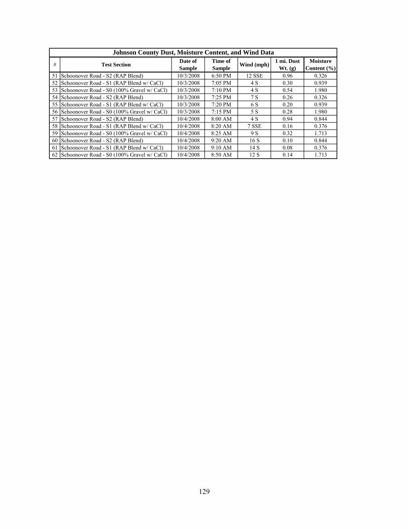
129

51 Schoonover Road - S2 (RAP Blend) 10/3/2008 6:50 PM 12 SSE 0.96 0.32652 Schoonover Road - S1 (RAP Blend w/ CaCl) 10/3/2008 7:05 PM 4 S 0.30 0.93953 Schoonover Road - S0 (100% Gravel w/ CaCl) 10/3/2008 7:10 PM 4 S 0.54 1.98054 Schoonover Road - S2 (RAP Blend) 10/3/2008 7:25 PM 7 S 0.26 0.32655 Schoonover Road - S1 (RAP Blend w/ CaCl) 10/3/2008 7:20 PM 6 S 0.20 0.93956 Schoonover Road - S0 (100% Gravel w/ CaCl) 10/3/2008 7:15 PM 5 S 0.28 1.98057 Schoonover Road - S2 (RAP Blend) 10/4/2008 8:00 AM 4 S 0.94 0.84458 Schoonover Road - S1 (RAP Blend w/ CaCl) 10/4/2008 8:20 AM 7 SSE 0.16 0.37659 Schoonover Road - S0 (100% Gravel w/ CaCl) 10/4/2008 8:25 AM 9 S 0.32 1.71360 Schoonover Road - S2 (RAP Blend) 10/4/2008 9:20 AM 16 S 0.10 0.84461 Schoonover Road - S1 (RAP Blend w/ CaCl) 10/4/2008 9:10 AM 14 S 0.08 0.37662 Schoonover Road - S0 (100% Gravel w/ CaCl) 10/4/2008 8:50 AM 12 S 0.14 1.713

Johnson County Dust, Moisture Content, and Wind Data



Wt. (g)Moisture

Content (%)

130

A.3 Laramie County Moisture Content Summary

Date Section Moisture, %June 9, 2008 A0 -G-U 2.6%June 17, 2008 A0 -G-U 1.0%June 24, 2008 A0 -G-U 5.0%July 28, 2008 A0 -G-U 1.2%July 29, 2008 A0 -G-U 0.7%

August 6, 2008 A0 -G-U 0.9%August 7, 2008 A0 -G-U 0.7%August 13, 2008 A0 -G-U 0.9%August 21, 2008 A0 -G-U 2.1%August 22, 2008 A0 -G-U 2.6%

September 5, 2008 A0 -G-U 2.9%September 18, 2008 A0 -G-U 1.2%

October 4, 2008 A0 -G-U 1.4%June 9, 2008 A1 -RAP/G-U 2.0%June 17, 2008 A1 -RAP/G-U 0.5%June 24, 2008 A1 -RAP/G-U 6.4%July 11, 2008 A1 -RAP/G-U 0.7%July 28, 2008 A1 -RAP/G-U 0.7%July 29, 2008 A1 -RAP/G-U 0.4%

August 6, 2008 A1 -RAP/G-U 0.5%August 7, 2008 A1 -RAP/G-U 0.4%August 13, 2008 A1 -RAP/G-U 0.6%August 21, 2008 A1 -RAP/G-U 1.6%August 22, 2008 A1 -RAP/G-U 0.5%

September 5, 2008 A1 -RAP/G-U 4.0%September 18, 2008 A1 -RAP/G-U 0.3%

October 4, 2008 A1 -RAP/G-U 1.0%

131

Date Section Moisture, %June 9, 2008 A2 -RAP/G-U 1.0%June 17, 2008 A2 -RAP/G-U 0.6%June 24, 2008 A2 -RAP/G-U 3.4%July 28, 2008 A2 -RAP/G-U 0.8%July 29, 2008 A2 -RAP/G-U 0.2%

August 6, 2008 A2 -RAP/G-U 0.5%August 7, 2008 A2 -RAP/G-U 0.4%August 13, 2008 A2 -RAP/G-U 0.5%August 21, 2008 A2 -RAP/G-U 1.3%August 22, 2008 A2 -RAP/G-U 0.5%

September 5, 2008 A2 -RAP/G-U 3.0%September 18, 2008 A2 -RAP/G-U 0.5%

October 4, 2008 A2 -RAP/G-U 0.5%June 9, 2008 P0 -G-U 2.5%June 17, 2008 P0 -G-U 1.3%June 24, 2008 P0 -G-U 5.5%July 28, 2008 P0 -G-U 1.2%July 29, 2008 P0 -G-U 0.6%

August 6, 2008 P0 -G-U 0.8%August 7, 2008 P0 -G-U 0.6%August 13, 2008 P0 -G-U 0.8%August 21, 2008 P0 -G-U 1.9%August 22, 2008 P0 -G-U 0.7%

September 5, 2008 P0 -G-U 2.7%September 18, 2008 P0 -G-U 1.3%

October 4, 2008 P0 -G-U 0.8%

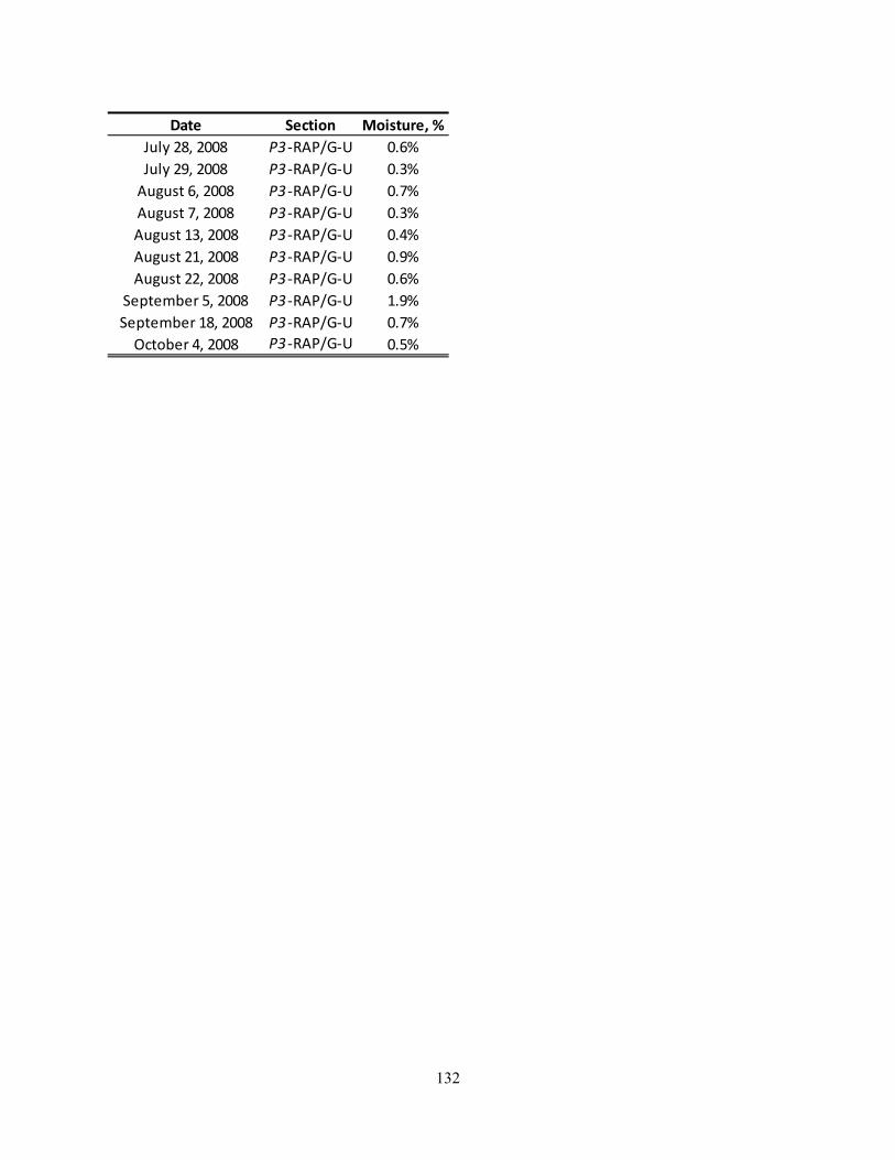
132

Date Section Moisture, %July 28, 2008 P3 -RAP/G-U 0.6%July 29, 2008 P3 -RAP/G-U 0.3%

August 6, 2008 P3 -RAP/G-U 0.7%August 7, 2008 P3 -RAP/G-U 0.3%August 13, 2008 P3 -RAP/G-U 0.4%August 21, 2008 P3 -RAP/G-U 0.9%August 22, 2008 P3 -RAP/G-U 0.6%

September 5, 2008 P3 -RAP/G-U 1.9%September 18, 2008 P3 -RAP/G-U 0.7%

October 4, 2008 P3 -RAP/G-U 0.5%

133

A.4 Johnson County Moisture Content Summary

Date Section Moisture, % CommentsJune 3, 2008 § 3.5%June 3, 2008 § 3.4%June 3, 2008 § 3.2%June 4, 2008 § 4.8%June 4, 2008 § 4.0%June 4, 2008 § 3.7%June 4, 2008 § 3.4%June 9, 2008 S0 -G-U 2.2%June 11, 2008 S0 -G-U 2.5%June 17, 2008 S0 -G-U 0.7%July 14, 2008 S0 -G-U 1.7%July 28, 2008 S0 -G-C 1.3%July 29, 2008 S0 -G-C 1.7%

August 6, 2008 S0 -G-C 0.7%August 7, 2008 S0 -G-C 1.5%August 21, 2008 S0 -G-C 1.3%August 22, 2008 S0 -G-C 1.8%

September 1, 2008 S0 -G-C 2.6%October 3, 2008 S0 -G-C 2.0%October 4, 2008 S0 -G-C 1.7%

§ Samples of blended RAP and Aggregate in the windrow after delivery from the stockpile to the roadway

Samples taken before calcium chloride applied

134

Date Section Moisture, %

June 9, 2008S1 -RAP/G-U &

S2 -RAP/G-U2.1%

June 11, 2008S1 -RAP/G-U &

S2 -RAP/G-U1.9%

June 17, 2008S1 -RAP/G-U &

S2 -RAP/G-U0.3%

July 28, 2008 S1 -RAP/G-C 0.3%July 29, 2008 S1 -RAP/G-C 0.5%

August 6, 2008 S1 -RAP/G-C 0.3%August 7, 2008 S1 -RAP/G-C 0.5%August 13, 2008 S1 -RAP/G-C 0.3%August 21, 2008 S1 -RAP/G-C 0.3%August 22, 2008 S1 -RAP/G-C 0.4%

September 1, 2008 S1 -RAP/G-C 0.4%October 3, 2008 S1 -RAP/G-C 0.3%October 4, 2008 S1 -RAP/G-C 0.8%

July 28, 2008 S2 -RAP/G-U 1.7%July 29, 2008 S2 -RAP/G-U 1.6%

August 6, 2008 S2 -RAP/G-U 1.3%August 7, 2008 S2 -RAP/G-U 1.1%August 13, 2008 S2 -RAP/G-U 0.7%August 21, 2008 S2 -RAP/G-U 1.3%August 22, 2008 S2 -RAP/G-U 1.3%

September 1, 2008 S2 -RAP/G-U 2.1%October 3, 2008 S2 -RAP/G-U 0.9%October 4, 2008 S2 -RAP/G-U 0.4%

Samples taken before calcium chloride applied

135

A.5 Sweetwater County Moisture Content Summary

Date MP Section MC, %April 27, 2011 0.30 A -CB-M 3.6%April 27, 2011 0.80 B -CB-M 4.1%

July 8, 2011 1.00 B -CB-M 2.2%July 8, 2011 1.50 D -CB-U 0.7%

August 10, 2011 1.00 B -CB-M 1.5%August 10, 2011 1.50 C -CB-ML 0.7%August 10, 2011 2.00 D -CB-ML 0.7%April 27, 2011 2.20 E -CTB-U 3.3%April 27, 2011 4.30 J -CTB-U 4.6%April 27, 2011 4.79 J -CTB-U 4.6%

July 8, 2011 2.70 F -CTB-U 1.9%July 8, 2011 3.80 H -CTB-U 2.7%

August 10, 2011 2.40 E -CTB-M 1.7%August 10, 2011 3.10 F -CTB-M 2.1%August 10, 2011 4.80 J -CTB-M 2.1%August 10, 2011 3.60 G -CTB-MP 1.4%August 10, 2011 4.10 H -CTB-MP 1.5%April 27, 2011 5.21 K -CTB/RAP-U 5.1%

August 10, 2011 5.30 K -CTB/RAP-M 1.7%April 27, 2011 9.00 R -N-U 7.2%April 27, 2011 9.50 S -N-U 7.3%April 27, 2011 5.71 L -RAP-U 5.7%April 27, 2011 6.29 M -RAP-U 5.2%April 27, 2011 6.73 N -RAP-U 3.3%April 27, 2011 7.22 P -RAP-U 6.5%April 27, 2011 7.78 Q -RAP-U 5.1%

July 8, 2011 6.20 M -RAP-U 1.2%

July 8, 2011 7.70 Q -RAP-U 7.4%Pothole: only place we could break up the crust with a pickaxe

August 10, 2011 7.00 N -RAP-M 1.9%August 10, 2011 6.00 L -RAP-MP 0.6%August 10, 2011 6.50 M -RAP-MP 0.9%August 10, 2011 7.50 P -RAP-U 0.2%

136

A.6 Laramie County Dustometer Measurement Summary

Date Section Leng

th, m

iles

Dire

ctio

n of

Tr

avel Speed,

mph Pass

es

Weather Tem

pera

ture

, ⁰F

Spee

d

Dire

ctio

n

g g/mile Comments

June 9, 2008 A1 -RAP/G-U 0.50 EB 40 1 Sunny 50 25 W 0.91 1.82fairly consistent winds of ~ 25 mph out of the West

June 9, 2008 A2 -RAP/G-U 0.50 WB 40 1 Sunny 50 25 W 3.10 6.20

fairly consistent winds of ~ 25 mph out of the West. Looks like larger coarse sized particles in collection. Screen is starting to open up.

June 9, 2008 A0 -G-U 0.50 WB 40 1 Sunny 50 25 W 2.89 5.78

fairly consistent winds of ~ 25 mph out of the West. Looks like larger coarse sized particles in collection. Screen flipped upside down to prevent coarse particles from entering.

June 9, 2008 P1- RAP/G-U 0.50 NB 40 1 Sunny 50 25 W 0.32 0.64June 9, 2008 P0 -G-U 0.50 NB 40 1 Sunny 50 25 W 0.19 0.38

June 17, 2008 A1 -RAP/G-U 0.50 EB 40 1 Sunny 65 8 W 1.93 3.86June 17, 2008 A2 -RAP/G-U 0.50 WB 40 1 Sunny 65 8 W 3.26 6.52June 17, 2008 A0 -G-U 0.50 EB 40 1 Sunny 65 8 W 1.88 3.76June 17, 2008 P1- RAP/G-U 0.50 NB 40 1 Sunny 65 8 W 0.44 0.88June 17, 2008 P0 -G-U 0.50 NB 40 1 Sunny 65 8 W 0.46 0.92June 24, 2008 A1 -RAP/G-U 0.50 EB 40 1 Sunny 68 8 WNW 1.20 2.40June 24, 2008 A2 -RAP/G-U 0.50 WB 40 1 Sunny 68 8 WNW 0.79 1.58June 24, 2008 A0 -G-U 0.50 EB 40 1 Sunny 68 8 WNW 1.20 2.40June 24, 2008 P1- RAP/G-U 0.50 NB 40 1 Sunny 68 8 WNW 1.17 2.34June 24, 2008 P0 -G-U 0.50 NB 40 1 Sunny 68 8 WNW 2.92 5.84

July 11, 2008 A1 -RAP/G-U 0.50 EB 40 1 Sunny 68 20 W 1.10 2.20

Consistent winds of 15 - 20 mph out of West. Gusts up to 30 mph. Hard to collect sample from box without it blowing away.

July 28, 2008 A1 -RAP/G-U 0.50 W 40 1 Partly Cloudy 75 16 WNW 0.38 0.76July 28, 2008 A2 -RAP/G-U 0.50 W 40 1 Partly Cloudy 75 20 W 0.21 0.42July 28, 2008 A0 -G-U 0.50 W 40 1 Partly Cloudy 75 20 WNW 0.48 0.96July 28, 2008 P1- RAP/G-U 0.50 S 40 1 Partly Cloudy 75 11 WNW 0.32 0.64July 28, 2008 P0 -G-U 0.50 S 40 1 Partly Cloudy 75 12 WNW 0.54 1.08July 28, 2008 A1 -RAP/G-U 0.50 E 40 1 Partly Cloudy 75 11 W 0.17 0.34July 28, 2008 A2 -RAP/G-U 0.50 E 40 1 Partly Cloudy 75 10 W 0.11 0.22July 28, 2008 A0 -G-U 0.50 E 40 1 Partly Cloudy 75 17 WNW 0.04 0.08July 28, 2008 P1- RAP/G-U 0.50 N 40 1 Partly Cloudy 75 13 WNW 0.12 0.24July 28, 2008 P0 -G-U 0.50 N 40 1 Partly Cloudy 75 14 WNW 0.18 0.36July 29, 2008 A1 -RAP/G-U 0.50 E 40 1 Overcast 80 5 W 0.33 0.66July 29, 2008 A2 -RAP/G-U 0.50 E 40 1 Overcast 80 7 W 0.40 0.80July 29, 2008 A0 -G-U 0.50 E 40 1 Overcast 80 6 W 0.37 0.74July 29, 2008 P1- RAP/G-U 0.50 N 40 1 Overcast 80 10 W 0.27 0.54July 29, 2008 P0 -G-U 0.50 S 40 1 Overcast 80 8 W 0.76 1.52July 29, 2008 A1 -RAP/G-U 0.50 W 40 1 Overcast 80 10 W 0.80 1.60July 29, 2008 A2 -RAP/G-U 0.50 W 40 1 Overcast 80 8 W 0.62 1.24July 29, 2008 A0 -G-U 0.50 W 40 1 Overcast 80 12 W 1.25 2.50July 29, 2008 P1- RAP/G-U 0.50 S 40 1 Overcast 80 11 W 0.42 0.84July 29, 2008 P0 -G-U 0.50 N 40 1 Overcast 80 9 W 0.90 1.80

No indications of recent precipitation in area.

Wind Dust Weight


Recent precipitation indicated by standing water in parts of roadway and ditches. Within past 24-48 hours. Shoulders were soft and wet.

No indications of recent rain in area. Looks and feels drier than previous days, but it still could dry out more.

fairly consistent winds of ~ 25 mph out of the West. This was a cross wind and

137

Date Section Leng

th, m

iles

Dire

ctio

n of

Tr

avel Speed,

mph Pass

es

Weather Tem

pera

ture

, ⁰F

Spee

d

Dire

ctio

n

g g/mile CommentsAugust 6, 2008 A0 -G-U 0.50 E 40 1 Partly Cloudy 65 15 NW 0.08 0.16August 6, 2008 P1- RAP/G-U 0.50 N 40 1 Partly Cloudy 65 16 NW 0.26 0.52August 6, 2008 P0 -G-U 0.50 N 40 1 Partly Cloudy 65 10 NW 0.99 1.98August 6, 2008 A1 -RAP/G-U 0.50 W 40 1 Partly Cloudy 65 12 NW 0.24 0.48August 6, 2008 A2 -RAP/G-U 0.50 W 40 1 Partly Cloudy 65 16 NW 0.35 0.70August 6, 2008 A0 -G-U 0.50 W 40 1 Partly Cloudy 65 15 NW 0.28 0.56August 6, 2008 P1- RAP/G-U 0.50 S 40 1 Partly Cloudy 65 11 NW 0.15 0.30August 6, 2008 P0 -G-U 0.50 S 40 1 Partly Cloudy 65 9 NW 0.63 1.26August 7, 2008 A1 -RAP/G-U 0.50 E 40 1 Partly Cloudy 85 11 S 0.20 0.40August 7, 2008 A2 -RAP/G-U 0.50 E 40 1 Partly Cloudy 85 10 S 0.22 0.44August 7, 2008 A0 -G-U 0.50 E 40 1 Partly Cloudy 85 7 SE 0.35 0.70August 7, 2008 P1- RAP/G-U 0.50 N 40 1 Partly Cloudy 85 8 SE 0.18 0.36August 7, 2008 P0 -G-U 0.50 N 40 1 Partly Cloudy 85 10 S 0.31 0.62August 7, 2008 A1 -RAP/G-U 0.50 W 40 1 Partly Cloudy 85 8 S 0.17 0.34August 7, 2008 A2 -RAP/G-U 0.50 W 40 1 Partly Cloudy 85 9 S 0.05 0.10August 7, 2008 A0 -G-U 0.50 W 40 1 Partly Cloudy 85 9 S 0.09 0.18August 7, 2008 P1- RAP/G-U 0.50 S 40 1 Partly Cloudy 85 12 S 0.20 0.40August 7, 2008 P0 -G-U 0.50 S 40 1 Partly Cloudy 85 15 S 0.22 0.44

August 13, 2008 A1 -RAP/G-U 0.50 E 40 1 Sunny 65 15 NW 0.15 0.30August 13, 2008 A2 -RAP/G-U 0.50 E 40 1 Sunny 65 7 WNW 0.05 0.10August 13, 2008 A0 -G-U 0.50 E 40 1 Sunny 65 12 NW 0.06 0.12August 13, 2008 P1- RAP/G-U 0.50 N 40 1 Sunny 65 11 NW 0.07 0.14August 13, 2008 P0 -G-U 0.50 N 40 1 Sunny 65 12 W 0.14 0.28August 13, 2008 A1 -RAP/G-U 0.50 W 40 1 Sunny 65 15 WNW 0.39 0.78August 13, 2008 A2 -RAP/G-U 0.50 W 40 1 Sunny 65 14 WNW 0.31 0.62August 13, 2008 A0 -G-U 0.50 W 40 1 Sunny 65 16 WNW 0.47 0.94August 13, 2008 P1- RAP/G-U 0.50 S 40 1 Sunny 65 13 WNW 0.38 0.76August 13, 2008 P0 -G-U 0.50 S 40 1 Sunny 65 10 NW 0.40 0.80August 21, 2008 A1 -RAP/G-U 0.50 E 40 1 Sunny 60 3 NW 0.60 1.20August 21, 2008 A2 -RAP/G-U 0.50 E 40 1 Sunny 60 4 NW 0.41 0.82August 21, 2008 A0 -G-U 0.50 E 40 1 Sunny 60 5 NW 1.35 2.70August 21, 2008 P1- RAP/G-U 0.50 N 40 1 Sunny 60 6 NW 0.18 0.36August 21, 2008 P0 -G-U 0.50 N 40 1 Sunny 60 5 WNW 0.42 0.84August 21, 2008 A1 -RAP/G-U 0.50 W 40 1 Sunny 60 5 NW 0.16 0.32August 21, 2008 A2 -RAP/G-U 0.50 W 40 1 Sunny 60 3 NW 0.14 0.28August 21, 2008 A0 -G-U 0.50 W 40 1 Sunny 60 4 WNW 0.34 0.68August 21, 2008 P1- RAP/G-U 0.50 S 40 1 Sunny 60 5 NW 0.60 1.20August 21, 2008 P0 -G-U 0.50 S 40 1 Sunny 60 4 NW 2.00 4.00

Wind Dust Weight





138

Date Section Leng

th, m

iles

Dire

ctio

n of

Tr

avel Speed,

mph Pass

es

Weather Tem

pera

ture

, ⁰F

Spee

d

Dire

ctio

n

g g/mileAugust 22, 2008 A0 -G-U 0.50 E 40 1 Sunny 75 11 NE 0.09 0.18August 22, 2008 P1- RAP/G-U 0.50 S 40 1 Sunny 75 14 NE 0.16 0.32August 22, 2008 P0 -G-U 0.50 S 40 1 Sunny 75 8 NE 0.76 1.52August 22, 2008 A1 -RAP/G-U 0.50 W 40 1 Sunny 75 8 NE 0.17 0.34August 22, 2008 A2 -RAP/G-U 0.50 W 40 1 Sunny 75 9 NE 0.24 0.48August 22, 2008 A0 -G-U 0.50 W 40 1 Sunny 75 11 NE 0.40 0.80August 22, 2008 P1- RAP/G-U 0.50 N 40 1 Sunny 75 9 NE 0.58 1.16August 22, 2008 P0 -G-U 0.50 N 40 1 Sunny 75 13 NE 1.49 2.98

September 5, 2008 A1 -RAP/G-U 0.50 E 40 1 Overcast 50 11 S 0.43 0.86September 5, 2008 A2 -RAP/G-U 0.50 E 40 1 Overcast 50 8 S 0.41 0.82September 5, 2008 A0 -G-U 0.50 E 40 1 Overcast 50 10 S 0.26 0.52September 5, 2008 P1- RAP/G-U 0.50 N 40 1 Overcast 50 13 S 0.47 0.94September 5, 2008 P0 -G-U 0.50 N 40 1 Overcast 50 12 S 0.47 0.94September 5, 2008 A1 -RAP/G-U 0.50 W 40 1 Overcast 50 12 S 0.11 0.22September 5, 2008 A2 -RAP/G-U 0.50 W 40 1 Overcast 50 7 S 0.13 0.26September 5, 2008 A0 -G-U 0.50 W 40 1 Overcast 50 8 S 0.15 0.30September 5, 2008 P1- RAP/G-U 0.50 S 40 1 Overcast 50 9 S 0.24 0.48September 5, 2008 P0 -G-U 0.50 S 40 1 Overcast 50 15 S 0.43 0.86

September 18, 2008 A1 -RAP/G-U 0.50 E 40 1 Partly Cloudy 70 12 SSW 0.70 1.40September 18, 2008 A2 -RAP/G-U 0.50 E 40 1 Partly Cloudy 70 11 SSW 0.46 0.92September 18, 2008 A0 -G-U 0.50 E 40 1 Partly Cloudy 70 13 SSW 0.80 1.60September 18, 2008 P1- RAP/G-U 0.50 N 40 1 Partly Cloudy 70 12 SSW 0.11 0.22September 18, 2008 P0 -G-U 0.50 N 40 1 Partly Cloudy 70 10 SSW 0.26 0.52September 18, 2008 A1 -RAP/G-U 0.50 W 40 1 Partly Cloudy 70 10 SSW 0.27 0.54September 18, 2008 A2 -RAP/G-U 0.50 W 40 1 Partly Cloudy 70 9 S 0.14 0.28September 18, 2008 A0 -G-U 0.50 W 40 1 Partly Cloudy 70 9 S 0.40 0.80September 18, 2008 P1- RAP/G-U 0.50 S 40 1 Partly Cloudy 70 8 S 0.77 1.54September 18, 2008 P0 -G-U 0.50 S 40 1 Partly Cloudy 70 7 S 1.09 2.18

October 4, 2008 A1 -RAP/G-U 0.50 W 40 1 Overcast 65 10 S 0.09 0.18October 4, 2008 A2 -RAP/G-U 0.50 W 40 1 Overcast 65 8 S 0.10 0.20October 4, 2008 A0 -G-U 0.50 W 40 1 Overcast 65 9 S 0.08 0.16October 4, 2008 P1- RAP/G-U 0.50 N 40 1 Overcast 65 13 S 0.38 0.76October 4, 2008 P0 -G-U 0.50 N 40 1 Overcast 65 11 S 0.77 1.54October 4, 2008 A1 -RAP/G-U 0.50 E 40 1 Overcast 65 11 S 0.28 0.56October 4, 2008 A2 -RAP/G-U 0.50 E 40 1 Overcast 65 10 S 0.29 0.58October 4, 2008 A0 -G-U 0.50 E 40 1 Overcast 65 10 S 0.38 0.76October 4, 2008 P1- RAP/G-U 0.50 S 40 1 Overcast 65 13 S 0.21 0.42October 4, 2008 P0 -G-U 0.50 S 40 1 Overcast 65 12 S 0.47 0.94




Wind Dust Weight


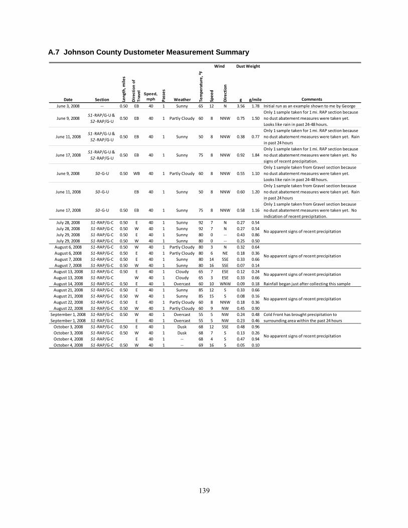
139

A.7 Johnson County Dustometer Measurement Summary

Date Section Leng

th, m

iles

Dire

ctio

n of

Tr

avel Speed,

mph Pass

es

Weather Tem

pera

ture

, ⁰F

Spee

d

Dire

ctio

n

g g/mile CommentsJune 3, 2008 -- 0.50 EB 40 1 Sunny 65 12 N 3.56 1.78 Initial run as an example shown to me by George

June 9, 2008S1 -RAP/G-U &

S2 -RAP/G-U0.50 EB 40 1 Partly Cloudy 60 8 NNW 0.75 1.50

Only 1 sample taken for 1 mi. RAP section because no dust abatement measures were taken yet. Looks like rain in past 24-48 hours.

June 11, 2008S1 -RAP/G-U &

S2 -RAP/G-U0.50 EB 40 1 Sunny 50 8 NNW 0.38 0.77

Only 1 sample taken for 1 mi. RAP section because no dust abatement measures were taken yet. Rain in past 24 hours

June 17, 2008S1 -RAP/G-U &

S2 -RAP/G-U0.50 EB 40 1 Sunny 75 8 NNW 0.92 1.84

Only 1 sample taken for 1 mi. RAP section because no dust abatement measures were taken yet. No signs of recent precipitation.

June 9, 2008 S0 -G-U 0.50 WB 40 1 Partly Cloudy 60 8 NNW 0.55 1.10Only 1 sample taken from Gravel section because no dust abatement measures were taken yet. Looks like rain in past 24-48 hours.

June 11, 2008 S0 -G-U EB 40 1 Sunny 50 8 NNW 0.60 1.20Only 1 sample taken from Gravel section because no dust abatement measures were taken yet. Rain in past 24 hours

June 17, 2008 S0 -G-U 0.50 EB 40 1 Sunny 75 8 NNW 0.58 1.16Only 1 sample taken from Gravel section because no dust abatement measures were taken yet. No indication of recent precipitation.

July 28, 2008 S1 -RAP/G-C 0.50 E 40 1 Sunny 92 7 N 0.27 0.54July 28, 2008 S1 -RAP/G-C 0.50 W 40 1 Sunny 92 7 N 0.27 0.54July 29, 2008 S1 -RAP/G-C 0.50 E 40 1 Sunny 80 0 -- 0.43 0.86July 29, 2008 S1 -RAP/G-C 0.50 W 40 1 Sunny 80 0 -- 0.25 0.50

August 6, 2008 S1 -RAP/G-C 0.50 W 40 1 Partly Cloudy 80 3 N 0.32 0.64August 6, 2008 S1 -RAP/G-C 0.50 E 40 1 Partly Cloudy 80 6 NE 0.18 0.36August 7, 2008 S1 -RAP/G-C 0.50 E 40 1 Sunny 80 14 SSE 0.33 0.66August 7, 2008 S1 -RAP/G-C 0.50 W 40 1 Sunny 80 16 SSE 0.07 0.14August 13, 2008 S1 -RAP/G-C 0.50 E 40 1 Cloudy 65 7 ESE 0.12 0.24August 13, 2008 S1 -RAP/G-C W 40 1 Cloudy 65 3 ESE 0.33 0.66August 14, 2008 S1 -RAP/G-C 0.50 E 40 1 Overcast 60 10 WNW 0.09 0.18 Rainfall began just after collecting this sampleAugust 21, 2008 S1 -RAP/G-C 0.50 E 40 1 Sunny 85 12 S 0.33 0.66August 21, 2008 S1 -RAP/G-C 0.50 W 40 1 Sunny 85 15 S 0.08 0.16August 22, 2008 S1 -RAP/G-C 0.50 E 40 1 Partly Cloudy 60 8 NNW 0.18 0.36August 22, 2008 S1 -RAP/G-C 0.50 W 40 1 Partly Cloudy 60 9 NW 0.45 0.90

September 1, 2008 S1 -RAP/G-C 0.50 W 40 1 Overcast 55 5 NW 0.24 0.48September 1, 2008 S1 -RAP/G-C E 40 1 Overcast 55 5 NW 0.23 0.46

October 3, 2008 S1 -RAP/G-C 0.50 E 40 1 Dusk 68 12 SSE 0.48 0.96October 3, 2008 S1 -RAP/G-C 0.50 W 40 1 Dusk 68 7 S 0.13 0.26October 4, 2008 S1 -RAP/G-C E 40 1 -- 68 4 S 0.47 0.94October 4, 2008 S1 -RAP/G-C 0.50 W 40 1 -- 69 16 S 0.05 0.10

No apparent signs of recent precipitation

Cold Front has brought precipitation to surrounding area within the past 24 hours


Wind Dust Weight




140

Date Section Leng

th, m

iles

Dire

ctio

n of

Tr

avel Speed,

mph Pass

es

Weather Tem

pera

ture

, ⁰F

Spee

d

Dire

ctio

n

g g/mile CommentsJuly 28, 2008 S2 -RAP/G-U 0.50 E 40 1 Sunny 92 7 N 0.13 0.26July 28, 2008 S2 -RAP/G-U 0.50 W 40 1 Sunny 92 7 N 0.24 0.48July 29, 2008 S2 -RAP/G-U 0.50 E 40 1 Sunny 80 0 -- 0.24 0.48July 29, 2008 S2 -RAP/G-U 0.50 W 40 1 Sunny 80 0 -- 0.25 0.50

August 6, 2008 S2 -RAP/G-U 0.50 W 40 1 Partly Cloudy 80 4 NE 0.14 0.28August 6, 2008 S2 -RAP/G-U 0.50 E 40 1 Partly Cloudy 80 2 N 0.11 0.22August 7, 2008 S2 -RAP/G-U 0.50 E 40 1 Sunny 80 15 SSE 0.16 0.32August 7, 2008 S2 -RAP/G-U 0.50 W 40 1 Sunny 80 18 SSE 0.10 0.20August 13, 2008 S2 -RAP/G-U 0.50 W 40 1 Cloudy 65 5 SE 0.10 0.20 No apparent signs of recent precipitationAugust 21, 2008 S2 -RAP/G-U 0.50 E 40 1 Sunny 85 18 S 0.08 0.16August 21, 2008 S2 -RAP/G-U 0.50 W 40 1 Sunny 85 13 S 0.06 0.12August 22, 2008 S2 -RAP/G-U 0.50 E 40 1 Partly Cloudy 60 6 NW 0.07 0.14August 22, 2008 S2 -RAP/G-U 0.50 W 40 1 Partly Cloudy 60 7 NW 0.09 0.18

September 1, 2008 S2 -RAP/G-U 0.50 W 40 1 Overcast 55 2 NW 0.15 0.30

September 1, 2008 S2 -RAP/G-U 0.50 E 40 1 Overcast 55 5 NW 0.06 0.12

October 3, 2008 S2 -RAP/G-U 0.50 E 40 1 Dusk 68 4 S 0.15 0.30October 3, 2008 S2 -RAP/G-U 0.50 W 40 1 Dusk 68 6 S 0.10 0.20October 4, 2008 S2 -RAP/G-U 0.50 E 40 1 -- 68 7 SSE 0.08 0.16October 4, 2008 S2 -RAP/G-U 0.50 W 40 1 -- 70 14 S 0.04 0.08

July 14, 2008 S0 -G-C 0.50 WB 40 1 Sunny 80 15 NNW 0.54 1.08 Taken from section 3 - Gravel with CaCl.July 28, 2008 S0 -G-C 0.50 E 40 1 Sunny 92 7 N 0.23 0.46July 28, 2008 S0 -G-C 0.50 W 40 1 Sunny 92 7 N 0.52 1.04July 29, 2008 S0 -G-C 0.50 E 40 1 Sunny 80 0 -- 0.76 1.52July 29, 2008 S0 -G-C 0.50 W 40 1 Sunny 80 0 -- 0.68 1.36

August 6, 2008 S0 -G-C 0.50 W 40 1 Partly Cloudy 80 3 NE 0.49 0.98August 6, 2008 S0 -G-C 0.50 E 40 1 Partly Cloudy 80 0 -- 0.25 0.50August 7, 2008 S0 -G-C 0.50 E 40 1 Sunny 80 12 SSE 0.84 1.68August 7, 2008 S0 -G-C 0.50 W 40 1 Sunny 80 17 SSE 0.45 0.90August 21, 2008 S0 -G-C 0.50 E 40 1 Sunny 85 10 S 0.07 0.14August 21, 2008 S0 -G-C 0.50 W 40 1 Sunny 85 11 S 0.06 0.12August 22, 2008 S0 -G-C 0.50 E 40 1 Partly Cloudy 60 9 WNW 0.10 0.20August 22, 2008 S0 -G-C 0.50 W 40 1 Partly Cloudy 60 10 NNW 0.14 0.28

September 1, 2008 S0 -G-C 0.50 W 40 1 Overcast 55 3 NW 0.10 0.20September 1, 2008 S0 -G-C 0.50 E 40 1 Overcast 55 4 NW 0.09 0.18

October 3, 2008 S0 -G-C 0.50 E 40 1 Dusk 68 4 S 0.27 0.54October 3, 2008 S0 -G-C 0.50 W 40 1 Dusk 68 5 S 0.14 0.28October 4, 2008 S0 -G-C 0.50 E 40 1 -- 68 9 S 0.16 0.32October 4, 2008 S0 -G-C 0.50 W 40 1 -- 70 12 S 0.07 0.14




Wind Dust Weight








141

A.8 Sweetwater County Dustometer Measurement and Visual Dust Rating Summary

Date Section grams g/mile BMP EMP Dire

ctio

n

Pass

ess

Weather Tem

pera

ture

mph Dire

ctio

n Visual Dust

Rating Rater08-Jul-11 A -CB-M 0.10 0.10 0.0 0.5 Both 2 Sunny 85 12 WSW N GH & HR

10-Aug-11 A -CB-M 0.05 0.05 0.0 0.5 Both 2 Sunny 79 2 NE N GH & JJ10-Aug-11 B -CB-M 0.04 0.03 0.5 1.1 Both 2 Sunny 79 2 NE N GH & JJ08-Sep-11 A -CB-M 0.04 0.04 0.0 0.5 Both 2 L JJ08-Sep-11 B -CB-M 0.03 0.03 0.5 1.1 Both 2 L JJ15-Sep-11 A -CB-M 0.05 0.05 0.0 0.5 Both 2 Sunny 64 5 WSW N GH15-Sep-11 A&B -CB-M 0.29 0.26 0.0 1.1 SB 1 Mostly Sunny 60 3 SSE N GH15-Sep-11 B -CB-M 0.02 0.02 0.5 1.1 Both 2 Sunny 64 5 WSW N GH08-Jul-11 C -CB-U 0.48 0.60 1.1 1.5 Both 2 Sunny 85 12 WSW M GH & HR08-Jul-11 D -CB-U 0.77 0.77 1.5 2.0 Both 2 Sunny 85 12 WSW M GH & HR

10-Aug-11 C -CB-ML 0.01 0.01 1.1 1.6 Both 2 Sunny 79 2 NE N GH & JJ10-Aug-11 D -CB-ML 0.01 0.01 1.6 2.1 Both 2 Sunny 79 2 NE N GH & JJ08-Sep-11 C -CB-ML 0.05 0.05 1.1 1.6 Both 2 78 6 SE L JJ08-Sep-11 D -CB-ML 0.22 0.22 1.6 2.1 Both 2 80 6 SE M JJ15-Sep-11 C -CB-ML 0.34 0.34 1.1 1.6 Both 2 Mostly Sunny 60 3 SSE N GH15-Sep-11 C -CB-ML 0.44 0.44 1.1 1.6 Both 2 Sunny 64 5 WSW N GH15-Sep-11 D -CB-ML 0.64 0.64 1.6 2.1 Both 2 Mostly Sunny 60 3 SSE H GH15-Sep-11 D -CB-ML 0.42 0.42 1.6 2.1 Both 2 Sunny 64 5 WSW H GH08-Jul-11 E -CTB-U 0.55 0.46 2.0 2.6 Both 2 Sunny 85 12 WSW M GH & HR08-Jul-11 F -CTB-U 0.33 0.41 2.6 3.0 Both 2 Sunny 85 12 WSW M GH & HR08-Jul-11 F&G -CTB-U 0.62 0.78 3.0 3.4 Both 2 Sunny 85 12 WSW M GH & HR

10-Aug-11 E -CTB-M 0.09 0.09 2.1 2.6 Both 2 Sunny 79 2 NE N GH & JJ10-Aug-11 F -CTB-M 0.18 0.15 2.6 3.2 Both 2 Sunny 79 2 NE M GH & JJ08-Sep-11 E -CTB-M 0.32 0.32 2.1 2.6 Both 2 H JJ08-Sep-11 F -CTB-M 1.09 0.91 2.6 3.2 Both 2 H JJ15-Sep-11 E -CTB-M 0.23 0.23 2.1 2.6 Both 2 Sunny 64 5 WSW L GH15-Sep-11 F -CTB-M 4.66 3.88 2.6 3.2 Both 2 Cloudy 53 3 NW H GH08-Jul-11 F&G -CTB-U 0.62 0.78 3.0 3.4 Both 2 Sunny 85 12 WSW M GH & HR08-Jul-11 G -CTB-U 0.69 0.86 3.4 3.8 Both 2 Sunny 85 12 WSW M GH & HR08-Jul-11 H -CTB-U 0.75 0.94 3.8 4.2 Both 2 Sunny 85 12 WSW M GH & HR

10-Aug-11 G -CTB-MP 0.2 0.20 3.2 3.7 Both 2 Sunny 79 2 NE M GH & JJ10-Aug-11 H -CTB-MP 0.24 0.24 3.7 4.2 Both 2 Sunny 79 2 NE L GH & JJ08-Sep-11 G -CTB-MP 0.65 0.65 3.2 3.7 Both 2 80 5 SE H JJ08-Sep-11 H -CTB-MP 0.73 0.73 3.7 4.2 Both 2 H JJ15-Sep-11 G -CTB-MP 3.59 3.59 3.2 3.7 Both 2 Cloudy 53 3 NW H GH15-Sep-11 G&H -CTB-MP 4.20 2.10 3.2 4.2 Both 2 Sunny 64 5 WSW H GH15-Sep-11 H -CTB-MP 4.68 4.68 3.7 4.2 Both 2 Cloudy 53 3 NW H GH

Raters: GH - George Huntington; HR - Harry Rocheville; JJ - Josh JonesVisual Dust Ratings: N - None; L - Low; M - Medium; H - High

WindDust Weight

142

Date Section grams g/mile BMP EMP Dire

ctio

n

Pass

ess

Weather Tem

pera

ture

mph Dire

ctio

n Visual Dust

Rating Rater08-Jul-11 J -CTB-U 0.51 0.64 4.2 4.6 Both 2 Sunny 85 12 WSW M GH & HR

10-Aug-11 J -CTB-M 0.28 0.20 4.2 4.9 Both 2 Sunny 79 2 NE L GH & JJ08-Sep-11 J -CTB-M 1.00 0.71 4.2 4.9 Both 2 H JJ15-Sep-11 J -CTB-M 5.68 4.06 4.2 4.9 Both 2 Cloudy 53 3 NW H GH15-Sep-11 J -CTB-M 2.04 1.46 4.2 4.9 Both 2 Sunny 64 5 WSW H GH08-Jul-11 K&L -RAP-U 0.26 0.33 5.4 5.8 Both 2 Sunny 85 12 WSW L GH & HR

10-Aug-11 K -CTB/RAP-M 0.07 0.05 4.9 5.6 Both 2 Sunny 79 2 NE L GH & JJ08-Sep-11 K -CTB/RAP-M 0.56 0.40 4.9 5.6 Both 2 82 3 E L JJ08-Jul-11 K&L -RAP-U 0.26 0.33 5.4 5.8 Both 2 Sunny 85 12 WSW L GH & HR08-Jul-11 L -RAP-U 0.13 0.16 5.8 6.2 Both 2 Sunny 85 12 WSW L GH & HR08-Jul-11 M -RAP-U 0.23 0.29 6.2 6.6 Both 2 Sunny 85 12 WSW L GH & HR

10-Aug-11 L -RAP-MP 0.06 0.06 5.6 6.1 Both 2 Sunny 79 2 NE N GH & JJ10-Aug-11 M -RAP-MP 0.05 0.05 6.1 6.6 Both 2 Sunny 79 2 NE N GH & JJ08-Sep-11 L -RAP-MP 0.24 0.24 5.6 6.1 Both 2 L JJ08-Sep-11 M -RAP-MP 0.19 0.19 6.1 6.6 Both 2 77 9 E L JJ15-Sep-11 L&M -RAP-MP 0.15 0.07 5.6 6.6 Both 2 Sunny 64 5 WSW L GH15-Sep-11 L -RAP-MP 0.42 0.42 5.6 6.1 Both 2 Cloudy 53 3 NW L GH15-Sep-11 M -RAP-MP 0.27 0.27 6.1 6.6 Both 2 Mostly Sunny 60 3 SSE L GH08-Jul-11 N&P -RAP-U 0.16 0.20 7.0 7.4 Both 2 Sunny 85 12 WSW L GH & HR08-Jul-11 N -RAP-U 0.14 0.18 6.6 7.0 Both 2 Sunny 85 12 WSW L GH & HR

10-Aug-11 N -RAP-M 0.12 0.10 6.6 7.2 Both 2 Sunny 79 2 NE N GH & JJ08-Sep-11 N -RAP-M 0.06 0.05 6.6 7.2 Both 2 74 6 L JJ15-Sep-11 N -RAP-M 0.17 0.14 6.6 7.2 Both 2 Mostly Sunny 60 3 SSE L GH15-Sep-11 N -RAP-M 0.09 0.07 6.6 7.2 Both 2 Sunny 64 5 WSW L GH10-Aug-11 P -RAP-U 0.14 0.18 7.2 7.6 Both 2 Sunny 79 2 NE L GH & JJ10-Aug-11 Q -RAP-U 0.15 0.19 7.6 8.0 Both 2 Sunny 79 2 NE L GH & JJ08-Sep-11 P -RAP-U 0.04 0.05 7.2 7.6 Both 2 81 6 E L JJ08-Sep-11 Q -RAP-U 0.03 0.04 7.6 8.0 Both 2 L JJ15-Sep-11 P -RAP-U 0.12 0.15 7.2 7.6 Both 2 Mostly Sunny 60 3 SSE L GH15-Sep-11 P -RAP-U 0.31 0.39 7.2 7.6 Both 2 Sunny 64 5 WSW L GH15-Sep-11 Q -RAP-U 0.64 0.80 7.6 8.0 Both 2 Mostly Sunny 60 3 SSE M GH15-Sep-11 Q -RAP-U 0.41 0.51 7.6 8.0 Both 2 Sunny 64 5 WSW M GH

Raters: GH - George Huntington; HR - Harry Rocheville; JJ - Josh JonesVisual Dust Ratings: N - None; L - Low; M - Medium; H - High

Dust Weight Wind

143

APPENDIX B. UNSURFACED ROAD CONDITION INDEXES

B.1 Laramie County URCI and Deduct Values

144

Date Section Cros

s Sec

tion

Road

side

Drai

nage

Was

hboa

rds/

Co

rrug

atio

ns

Dust

Poth

oles

Ruts

Loos

e Ag

greg

ate

URCI ConditionJune 24, 2008 A0 -G-U 0 0 0 0 0 0 0 100 ExcellentJuly 11, 2008 A0 -G-U 0 0 0 0 0 0 0 100 ExcellentJuly 28, 2008 A0 -G-U 0 0 0 0 0 0 0 100 Excellent

August 6, 2008 A0 -G-U 0 0 0 0 0 0 0 100 ExcellentAugust 13, 2008 A0 -G-U 0 0 0 0 0 0 0 100 ExcellentAugust 22, 2008 A0 -G-U 0 0 0 0 0 0 7 93 Excellent

September 5, 2008 A0 -G-U 0 0 0 0 0 0 7 93 ExcellentSeptember 18, 2008 A0 -G-U 0 0 0 0 0 0 6 94 Excellent

October 4, 2008 A0 -G-U 0 0 0 0 0 0 4 96 ExcellentJune 24, 2008 P0 -G-U 0 0 0 0 0 0 0 100 ExcellentJuly 11, 2008 P0 -G-U 0 0 0 0 0 0 0 100 ExcellentJuly 28, 2008 P0 -G-U 0 0 0 0 0 0 0 100 Excellent

August 6, 2008 P0 -G-U 0 0 0 0 0 0 0 100 ExcellentAugust 13, 2008 P0 -G-U 0 0 0 0 0 0 0 100 ExcellentAugust 22, 2008 P0 -G-U 0 0 0 0 0 0 0 100 Excellent

September 5, 2008 P0 -G-U 0 0 0 0 0 0 0 100 ExcellentSeptember 18, 2008 P0 -G-U 0 0 0 0 0 0 0 100 Excellent

October 4, 2008 P0 -G-U 0 0 0 0 0 0 0 100 ExcellentJune 24, 2008 A1 -RAP/G-U 0 2 0 0 0 3 9 86 ExcellentJuly 11, 2008 A1 -RAP/G-U 0 2 0 0 0 10 10 84 Very GoodJuly 28, 2008 A1 -RAP/G-U 0 0 0 0 0 1 10 89 Excellent

August 6, 2008 A1 -RAP/G-U 0 0 0 0 0 4 14 82 Very GoodAugust 13, 2008 A1 -RAP/G-U 0 0 0 0 0 4 15 81 Very GoodAugust 22, 2008 A1 -RAP/G-U 0 0 0 0 1 7 16 82 Very Good

September 5, 2008 A1 -RAP/G-U 0 0 0 0 1 7 18 86 ExcellentSeptember 18, 2008 A1 -RAP/G-U 0 0 0 0 1 6 16 77 Very Good

October 4, 2008 A1 -RAP/G-U 0 0 0 0 1 6 13 85 ExcellentJune 24, 2008 A2 -RAP/G-U 0 0 0 0 0 0 0 100 ExcellentJuly 11, 2008 A2 -RAP/G-U 0 0 0 0 0 0 4 96 ExcellentJuly 28, 2008 A2 -RAP/G-U 0 0 0 0 0 0 9 91 Excellent

August 6, 2008 A2 -RAP/G-U 0 0 0 0 0 0 11 89 ExcellentAugust 13, 2008 A2 -RAP/G-U 0 0 0 0 0 0 11 89 ExcellentAugust 22, 2008 A2 -RAP/G-U 0 0 0 0 0 0 11 89 Excellent

September 5, 2008 A2 -RAP/G-U 0 0 0 0 0 0 11 89 ExcellentSeptember 18, 2008 A2 -RAP/G-U 0 0 0 0 0 0 11 89 Excellent

October 4, 2008 A2 -RAP/G-U 0 0 0 0 0 0 11 89 ExcellentJune 24, 2008 P1 -RAP/G-U 0 0 0 0 0 0 6 94 ExcellentJuly 11, 2008 P1 -RAP/G-U 0 0 0 0 0 0 6 94 ExcellentJuly 28, 2008 P1 -RAP/G-U 0 0 0 0 0 0 11 89 Excellent

August 6, 2008 P1 -RAP/G-U 0 0 0 0 0 0 11 89 ExcellentAugust 13, 2008 P1 -RAP/G-U 0 0 0 0 0 0 11 89 ExcellentAugust 22, 2008 P1 -RAP/G-U 0 0 0 0 0 0 11 89 Excellent

September 5, 2008 P1 -RAP/G-U 0 0 0 0 0 0 11 89 ExcellentSeptember 18, 2008 P1 -RAP/G-U 0 0 0 0 0 0 9 91 Excellent

October 4, 2008 P1 -RAP/G-U 0 0 0 0 0 10 11 84 Very Good

Deduct Values

145

B.2 Johnson County URCI and Deduct Values

Date Section Cros

s Sec

tion

Road

side

Drai

nage

Was

hboa

rds/

Co

rrug

atio

ns

Dust

Poth

oles

Ruts

Loos

e Ag

greg

ate

URCI ConditionJuly 14, 2008 S1 -RAP/G-C 0 0 0 0 0 0 0 100 ExcellentJuly 29, 2008 S1 -RAP/G-C 0 0 0 0 0 0 0 100 Excellent

August 6, 2008 S1 -RAP/G-C 0 0 0 0 0 8 2 90 ExcellentAugust 13, 2008 S1 -RAP/G-C 0 0 0 0 0 8 3 89 ExcellentAugust 21, 2008 S1 -RAP/G-C 0 0 0 0 0 12 7 86 Excellent

September 1, 2008 S1 -RAP/G-C 0 0 0 0 0 9 12 84 Very GoodOctober 4, 2008 S1 -RAP/G-C 0 0 0 0 0 7 9 88 Excellent

July 14, 2008 S2 -RAP/G-U 0 0 0 0 0 0 0 100 ExcellentJuly 29, 2008 S2 -RAP/G-U 0 0 0 0 0 0 7 93 Excellent

August 6, 2008 S2 -RAP/G-U 0 0 0 0 0 0 7 93 ExcellentAugust 13, 2008 S2 -RAP/G-U 0 0 0 0 0 0 7 93 ExcellentAugust 21, 2008 S2 -RAP/G-U 0 0 0 0 0 0 9 91 Excellent

September 1, 2008 S2 -RAP/G-U 0 0 0 0 0 0 11 89 ExcellentOctober 4, 2008 S2 -RAP/G-U 0 0 0 0 0 0 7 93 Excellent

July 14, 2008 S0- G-C 0 0 0 0 0 0 0 100 ExcellentJuly 29, 2008 S0- G-C 0 0 0 0 0 5 0 95 Excellent

August 6, 2008 S0- G-C 0 0 0 0 0 5 8 90 ExcellentAugust 21, 2008 S0- G-C 0 0 0 0 0 11 10 85 Excellent

September 1, 2008 S0- G-C 0 0 0 0 0 11 12 83 Very GoodOctober 4, 2008 S0- G-C 0 0 24 0 0 29 12 64 Good

Deduct Values

146

B.3 Sweetwater County URCI and Deduct Values

Date BMP EMP Section Cros

s Sec

tion

Road

side

Drai

nage

Was

hboa

rds/

Co

rrug

atio

ns

Dust

Poth

oles

Ruts

Loos

e Ag

greg

ate

URCI Condition CommentApril 27, 2011 0.20 0.30 A -CB-M 0 0 4 2 0 0 0 94 Excellent 8 GoodJuly 7, 2011 0.36 0.40 A -CB-M 0 0 0 0 0 0 0 100 Excellent 9 Very Good

August 10, 2011 0.46 0.50 A -CB-M 0 0 0 0 0 0 0 100 Excellent 8 GoodSeptember 8, 2011 A -CB-M 0 0 8 2 0 1 0 89 Excellent 8 Good

April 27, 2011 0.70 0.80 B -CB-M 0 0 9 2 0 0 0 90 Excellent 8 GoodJuly 7, 2011 0.96 1.00 B -CB-M 0 0 0 0 0 0 0 100 Excellent 9 Very Good

August 10, 2011 0.96 1.00 B -CB-M 0 0 0 0 0 0 0 100 Excellent 8 GoodSeptember 8, 2011 B -CB-M 0 0 13 2 5 0 0 85 Excellent 8 Good

April 27, 2011 1.20 1.30 C -CB-U 0 0 2 2 0 0 16 80 Very Good 7 GoodJuly 7, 2011 1.36 1.40 C -CB-U 0 0 22 4 0 0 16 69 Good 6 Fair

August 10, 2011 1.46 1.50 C -CB-ML 0 0 0 0 0 0 0 100 Excellent 8 GoodSeptember 8, 2011 C -CB-ML 0 0 2 2 3 1 0 92 Excellent 9 Very Good

July 7, 2011 1.86 1.90 D -CB-U 0 0 1 4 0 0 14 81 Very Good 6 FairAugust 10, 2011 1.96 2.00 D -CB-ML 0 0 0 0 0 0 0 100 Excellent 7 Good

September 8, 2011 D -CB-ML 0 0 1 4 0 1 0 94 Excellent 8 GoodApril 27, 2011 2.20 2.30 E -CTB-U 0 0 6 2 0 4 16 78 Very Good 7 GoodJuly 7, 2011 2.36 2.40 E -CTB-U 0 0 24 4 0 0 13 78 Very Good 6 Fair

August 10, 2011 2.36 2.40 E -CTB-M 0 0 0 0 1 3 0 96 Excellent 7.5 GoodSeptember 8, 2011 E -CTB-M 0 0 1 15 5 7 8 83 Very Good 8 Good

April 27, 2011 2.80 2.90 F -CTB-U 0 0 8 2 3 0 17 78 Very Good 6 FairJuly 7, 2011 2.86 2.90 F -CTB-U 0 0 4 4 0 5 13 74 Very Good 6 Fair

August 10, 2011 3.06 3.10 F -CTB-M 0 0 8 4 0 6 12 83 Very Good 7 GoodSeptember 8, 2011 F -CTB-M 0 0 23 15 0 0 17 65 Good 7 Good

April 27, 2011 3.20 3.30 G -CTB-U 0 0 24 4 0 0 17 67 Good 6 FairJuly 7, 2011 3.66 3.70 G -CTB-U 0 0 32 4 0 0 13 69 Good 6 FairJuly 7, 2011 3.26 3.30 G -CTB-U 0 0 38 4 0 2 17 66 Good 5 Fair

August 10, 2011 3.56 3.60 G -CTB-MP 0 0 9 4 0 0 16 78 Very Good 7 GoodSeptember 8, 2011 G -CTB-MP 0 0 19 15 0 0 17 68 Good 7 Good

April 27, 2011 3.70 3.80 H -CTB-U 0 0 8 4 2 1 16 77 Very Good 6 FairJuly 7, 2011 4.06 4.10 H -CTB-U 0 0 33 4 0 0 13 68 Good 5 Fair

August 10, 2011 4.06 4.10 H -CTB-MP 0 0 7 2 0 12 7 83 Very Good 7 GoodSeptember 8, 2011 H -CTB-MP 0 0 8 15 0 7 17 77 Very Good 7 Good

April 27, 2011 4.20 4.30 J -CTB-U 0 0 21 4 0 0 26 69 Good 6 FairApril 27, 2011 4.70 4.80 J -CTB-U 0 0 14 4 0 0 10 78 Very Good 6 FairJuly 7, 2011 4.86 4.90 J -CTB-U 0 0 17 4 1 14 13 74 Very Good 7 GoodJuly 7, 2011 4.46 4.50 J -CTB-U 0 0 26 4 0 0 12 69 Good 6 Fair

August 10, 2011 4.76 4.80 J -CTB-M 0 0 3 2 2 14 7 78 Very Good 7 GoodSeptember 8, 2011 J -CTB-M 0 0 2 15 0 16 17 69 Good 7 Good

April 27, 2011 5.20 5.30 K -CTB/RAP-U 0 0 5 4 0 0 17 81 Very Good 7 GoodAugust 10, 2011 5.36 5.40 K -CTB/RAP-M 0 0 0 2 6 12 7 85 Excellent 8.5 Good/Very Good

September 8, 2011 K -CTB/RAP-M 0 0 0 2 1 3 0 94 Excellent 7 GoodApril 27, 2011 5.70 5.80 L -RAP-U 0 0 5 2 0 0 16 83 Very Good 7 GoodJuly 7, 2011 6.06 6.10 L -RAP-U 0 0 4 2 8 4 13 77 Very Good 7 GoodJuly 7, 2011 5.66 5.70 L -RAP-U 0 0 1 2 1 4 18 74 Very Good 6 Fair

August 10, 2011 5.96 6.00 L -RAP-MP 0 0 4 0 0 16 13 75 Very Good 7.5 GoodSeptember 8, 2011 L -RAP-MP 0 0 4 2 5 7 0 87 Excellent 7 Good

April 27, 2011 6.20 6.30 M -RAP-U 0 0 4 2 0 0 17 77 Very Good 8 GoodJuly 7, 2011 6.46 6.50 M -RAP-U 0 0 0 2 3 0 13 82 Very Good 7 Good

August 10, 2011 6.46 6.50 M -RAP-MP 0 0 0 0 1 0 0 99 Excellent 7.5 GoodSeptember 8, 2011 M -RAP-MP 0 0 0 2 1 10 0 87 Excellent 8 Good

April 27, 2011 6.70 6.80 N -RAP-U 0 0 19 2 0 0 23 73 Very Good 6 FairJuly 7, 2011 6.85 6.89 N -RAP-U 0 0 0 2 0 0 14 84 Very Good 7 Good

August 10, 2011 7.06 7.10 N -RAP-M 0 0 0 0 1 9 0 90 Excellent 8.5 Good/Very GoodSeptember 8, 2011 N -RAP-M 0 0 0 2 3 12 0 83 Very Good 8 Good

April 27, 2011 7.20 7.30 P -RAP-U 0 0 3 2 0 0 16 79 Very Good 8 GoodJuly 7, 2011 7.26 7.30 P -RAP-U 0 0 0 2 4 0 13 81 Very Good 7 Good

August 10, 2011 7.46 7.50 P -RAP-U 0 0 4 2 1 2 14 77 Very Good 6.5 Fair/GoodSeptember 8, 2011 P -RAP-U 0 0 0 2 2 3 0 93 Excellent 8 Good

April 27, 2011 7.70 7.80 Q-RAP-U 0 0 9 2 0 0 17 78 Very Good 7 GoodJuly 7, 2011 7.66 7.70 Q-RAP-U 0 0 0 2 0 0 13 85 Excellent 7 Good

August 10, 2011 7.86 7.90 Q -RAP-U 0 0 9 2 0 0 14 82 Very Good 6 FairSeptember 8, 2011 Q -RAP-U 0 0 0 2 0 7 0 91 Excellent 8 Good

April 27, 2011 8.90 9.00 R -N-U 0 0 4 2 0 15 0 79 Very Good 6 FairApril 27, 2011 9.40 9.50 S -N-U 0 0 6 2 2 22 0 77 Very Good 5 Fair

MgCl2

applied July 19, 2011

MgCl2


MgCl2/ polymer blend applied July 21, 2011

MgCl2


MgCl2

applied July 20,

MgCl2/ polymer blend applied July 20, 2011

Deduct Values

Ride Quality

MgCl2

applied June 28, 2011

MgCl2/ lignin blend applied July 21, 2011

147

APPENDIX C. GRADATIONS

C.1 Laramie County Gradations (% Passing)

A2 -RAP/G-U A1 -RAP/G-U P3- RAP/G-U2" 50 100 100 100

1½" 37.5 98 100 100 100 1001" 25 95 97 98 100 100

3/4" 19 92 95 96 99 1001/2" 12.5 80 82 84 97 943/8" 9.5 76 76 80 95 90#4 4.75 54 54 58 77 69#8 2.36 41 40 44 65 55#16 1.18 31 30 33 56 43#30 0.600 24 23 25 47 33#50 0.300 17 17 18 38 24

#100 0.150 11 11 12 31 17#200 0.075 7.6 7.4 8.4 23.0 11.2

Roadway SamplesLaramie County Gravel

Laramie County

RAP Blend After

ExtractionSieveSize, mm

148

C.2 Johnson County Gradations (% Passing)

SieveSize, mm Jo

hnso

n Co

Gra

vel

John

son

Co R

AP B

lend

Af

ter E

xtra

ctio

n

1½" 37.5 100 1001" 25 100 100

3/4" 19 98 991/2" 12.5 84 813/8" 9.5 76 76#4 4.75 62 55#8 2.36 52 47

#16 1.18 45 36#30 0.600 37 26#50 0.300 26 17#100 0.150 17 11#200 0.075 11.6 6.7

149

C.3 Sweetwater County Gradations (% Passing)

Milepost 1.7 1.8 2.1 2.3 2.9 3.1 3.8Section D -CB-U D -CB-U D&E -CB/CTB-U E -CTB-U F -CTB-U F -CTB-U H -CTB-U

Material CB CB W/CTB CTB CTB CTB CTBSieve Size, mm

1" 25.4 97% 99% 99% 95% 98% 97% 97%3/4" 19.0 88% 93% 97% 93% 94% 93% 93%1/2" 12.5 73% 81% 89% 83% 82% 83% 81%3/8" 9.5 64% 73% 82% 76% 72% 73% 71%#4 4.75 48% 57% 62% 57% 49% 47% 49%#8 2.36 38% 44% 50% 45% 36% 33% 34%

#30 0.600 24% 28% 29% 22% 18% 12% 16%#50 0.300 21% 22% 15% 9% 9% 7% 8%

#100 0.150 14% 12% 5% 3% 4% 3% 4%#200 0.075 6.6% 4.2% 1.7% 1.1% 1.5% 1.6% 2.3%

CB: WYDOT Grading W Crushed BaseCTB: Milled Cement-Treated Base (typically 8% - 9% portland cement)U: Not treated with dust suppressant

All materials listed above are non-plastic

Percent Passing

150

Milepost 4.6 4.6 4.8 4.9 5.1 5.2 5.3Section J -CTB-U J -CTB-U J -CTB-U J -CTB-U K -CTB/RAP-U K -CTB/RAP-U K -CTB/RAP-U

Material CTB CTB CTB CTB CTB/RAP CTB/RAP CTB/RAPSieve Size, mm

1" 25.4 99% 94% 97% 98% 98% 100% 100%3/4" 19.0 95% 89% 91% 94% 97% 95% 94%1/2" 12.5 87% 76% 79% 86% 88% 80% 84%3/8" 9.5 78% 66% 67% 78% 78% 67% 73%#4 4.75 54% 41% 41% 57% 50% 37% 43%#8 2.36 41% 30% 29% 43% 38% 20% 28%

#30 0.600 22% 13% 13% 22% 18% 8% 8%#50 0.300 12% 7% 7% 12% 11% 4% 2%

#100 0.150 6% 3% 3% 6% 5% 2% 1%#200 0.075 2.9% 1.0% 1.4% 2.7% 3.0% 0.9% 0.3%

RAP: Milled Reclaimed Asphalt PavementU: Not treated with dust suppressantCTB: Milled Cement-Treated Base (typically 8% - 9% portland cement)


Percent Passing

Milepost 6.0 6.3 6.5 6.7 7.0 7.7Section L -RAP-U M -RAP-U M -RAP-U N -RAP-U N -RAP-U Q -RAP-U

Material RAP RAP RAP RAP RAP RAPSieve Size, mm

1" 25.4 100% 100% 100% 100% 100% 98%3/4" 19.0 99% 95% 98% 98% 97% 95%1/2" 12.5 89% 80% 91% 88% 90% 85%3/8" 9.5 79% 67% 84% 78% 80% 77%#4 4.75 43% 37% 55% 46% 39% 47%#8 2.36 26% 20% 33% 24% 25% 29%

#30 0.600 6% 8% 12% 6% 7% 7%#50 0.300 3% 4% 5% 2% 3% 2%

#100 0.150 1% 2% 2% 0% 1% 0%#200 0.075 0.3% 0.9% 0.9% 0.2% 0.3% 0.2%

RAP: Milled Reclaimed Asphalt PavementU: Not treated with dust suppressant


Percent Passing

151

APPENDIX D. TRAFFIC AND OTHER DATA

D.1 Johnson and Laramie County General Section Data

D.2 Johnson County Traffic Data

Section County Road RAP %CaCl, psy

R-Value LL PI

CV, psi ADT

Heavy Trucks

85th%, MPH

Blending Method

Surfacing Date CaCl Date

A0 Laramie Atlas 0 -- 19 27 12 392 50 3% 55 -- April 14, 2008 --A2 Laramie Atlas 71 -- 78 -- -- -- 50 3% 55 Blade April 28, 2008 --A1 Laramie Atlas 82 -- 73 -- -- -- 50 3% 55 Blade April 29, 2008 --P0 Laramie Pry 0 -- 26 27 11 164 50 12% 56 -- April 14, 2008 --P1 Laramie Pry 69 -- 68 -- -- -- 50 12% 56 Blade May 1, 2008 --S2 Johnson Schoonover 50 -- -- -- -- -- 188 74% 51 Pugmill June 3, 2008 --S1 Johnson Schoonover 50 1.64 -- -- -- -- 188 74% 51 Pugmill June 4, 2008 June 19, 2008S0 Johnson Schoonover 0 1.64 -- 24 5 -- 188 74% 51 -- May 12, 2008 June 19, 2008

24-Hour Combined Traffic

VolumeTue, 6/10/2008 275Wed, 6/11/2008 261Thu, 6/12/2008 240Fri, 6/13/2008 275

Mon, 6/16/2008 266Tue, 6/17/2008 270Wed, 6/18/2008 276Thu, 6/19/2008 247Fri, 6/20/2008 151

Mon, 6/23/2008 225Tue, 6/24/2008 230Wed, 6/25/2008 264Thu, 6/26/2008 176Fri, 6/27/2008 136

Mon, 6/30/2008 262

Average 236.93Standard Deviation 46.21

Schoonover Road85th Percentile Speed, MPH

Maximum Speed, MPH Cars Pickups Trucks

Overall ADT

51.4 85.1 114 914 2944 188.02.9% 23.0% 74.1%

Class Cars & Trailer 2 Axle Long Buses2 Axle 6 Tire

3 Axle Single

4 Axle Single

< 5 Axle Double

5 Axle Double

>6 Axle Double

<6 Axle Multi

6 Axle Multi

>6 Axle Multi

Count 114 914 49 1857 301 9 285 337 95 0 2 9Percent 2.9% 23.0% 1.2% 46.8% 7.6% 0.2% 7.2% 8.5% 2.4% 0.0% 0.1% 0.2%

Vehicle Classification

Vehicle Classification Breakdown

153

APPENDIX E. ABBREVIATIONS

Abbreviation DescriptionAASHTO American Association of State Highway and Transportation Officials

ASTM American Society for Testing and MaterialsC treated with calcium chloride

CaCl2 calcium chlorideCB crushed baseCR County Road

CRREL Cold Regions Research & Engineering LaboratoryCSU Colorado State UniversityCTB cement-treated baseDOT Department of Transportation

FHWA Federal Highway Administrationft3 cubic feetg gramG gravel or aggregategal gallon

HMA hot mix asphaltHPM hot plant mix

HPMP hot plant mix pavementI-25 Interstate Highway 25I-80 Interstate Highway 80I-90 Interstate Highway 90JO Johnson CountyLA loose aggregate

lbs, lb pounds, poundLM 1:1 lignin sulfonate and magnesium chloride brine

LTAP local technical assistance programm meterM magnesium chloride brine

MgCl2 magnesium chloridemi miles

mm millimetersmph miles per hourMSE mechanically stabilized earth (retaining walls)NaCl sodium chloride

PASER Pavement Surface Evaluation and Rating

154

Abbreviation DescriptionPM 1:1 proprietary polymer and magnesium chloride brine

PM-10 particulate matter smaller than 10 μmpsi pounds per square inch

RAP reclaimed or recycled asphalt pavementRHPM RAP in hot plant mixRPM recycled pavement materialSH State HighwaySW Sweetwater CountyU untreated with dust suppressant

URCI Unsurfaced Road Condition IndexUSACE United States Army Corps of EngineersUSDOT United States Department of TransportationUSEPA United States Environmental Protection Agency

vpd vehicles per daywt weight

WYDOT Wyoming Department of Transportationyd2 square yardμm micron or micrometer

Performance of Reclaimed Asphalt Pavement on Unpaved … · · 2013-05-22Performance of Reclaimed...

Documents

Transcript of Performance of Reclaimed Asphalt Pavement on Unpaved … · · 2013-05-22Performance of Reclaimed...