Performance of particle in cell methods on highly ...

Performance of particle in cell methods on highly

concurrent computational architectures

M.F.Adams1 , S. Ethier2 and N. Wichmann3

1 Columbia University, APAM, 500 W. 120th St. Rm 200, MC 4701, New York, NY 10027,USA ([email protected])2 Princeton Plasma Physics Laboratory3 Cray Inc.

Abstract. Particle in cell (PIC) methods are effective in computing Vlasov-Poisson systemof equations used in simulations of magnetic fusion plasmas. PIC methods use grid basedcomputations, for solving Poisson’s equation or more generally Maxwell’s equations, as wellas Monte-Carlo type methods to sample the Vlasov equation. The presence of two types ofdiscretizations, deterministic field solves and Monte-Carlo methods for the Vlasov equation,pose challenges in understanding and optimizing performance on today large scale computerswhich require high levels of concurrency. These challenges arises from the need to optimizetwo very different types of processes and the interactions between them. Modern cache basedhigh-end computers have very deep memory hierarchies and high degrees of concurrency whichmust be utilized effectively to achieve good performance. The effective use of these machinesrequires maximizing concurrency by eliminating serial or redundant work and minimizingglobal communication. A related issue is minimizing the memory traffic between levels of thememory hierarchy because performance is often limited by the bandwidths and latencies of thememory system. This paper discusses some of the performance issues, particularly in regard toparallelism, of PIC methods. The gyrokinetic toroidal code (GTC) is used for these studies anda new radial grid decomposition is presented and evaluated. Scaling of the code is demonstratedon ITER sized plasmas with up to 16K Cray XT3/4 cores.

1. IntroductionA plasma is a gas with a high enough temperature that electrons are striped from the atoms

resulting in at least two species of particles (eg, electrons and deuterium ions). The Vlasovequation governs the behavior of each species in a plasma.

∂fα

∂t+ v · ∇fα +

qα

mα(E + v ×B)

∂fα

∂v= Cα,β(fα), (1)

where fα ≡ fα(x,v, t) is the distribution function which represents the density of particles ofspecies α found at any point in the domain of six-dimensional phase space (x,v); and Cαβ(f)is the Fokker-Planck collision term between species α and β. The term q(E + v × B) is theLorentz force due to electric and magnetic fields. A collisionless plasma is described by thisVlasov equation, without the Fokker-Plank term, along with Maxwell’s equations, or in our casesimply Poisson’s equation.

An effective method for analyzing the Vlasov-Poisson system of equations, used in simulatingfully ionized plasmas, is the particle in cell (PIC) method. PIC methods evolve plasma dynamics

SciDAC 2007 IOP PublishingJournal of Physics: Conference Series 78 (2007) 012001 doi:10.1088/1742-6596/78/1/012001

c© 2007 IOP Publishing Ltd 1

self-consistently by alternately pushing charged particles and solving the fields governed byMaxwell’s equations. These methods enable the study of plasma microturbulence on globalscales. This microturbulence (eg, scales of a few millimeters to centimeters or even larger)is important in understanding transport phenomenon in magnetically confined plasmas and isbest understood with a model that includes the effect of gyro motion of charged particles inmagnetic fields. The basic idea behind the gyrokinetic simulation method is to time-averagerapid precessing motions, and only to push the guiding center motion for the particles [1]. Thefinite Larmor (gyro) radius effects also enter the system through the gyrokinetic Poisson equation[1, 2].

The gyrokinetic Poisson equation which with some simplification is of the form:

τ

λ2D

(Φ− Φ

)= 4πe

( ¯δni − δne)

(2)

where Φ is the electrostatic potential, δni and δne are the fluctuation part of the ion and theelectron guiding center charge density, τ is the ratio of electron to ion temperature (assumed tobe 1.0 herein), λD is the Debey length, and Φ is the second gyro-phase averaged potential [2].With the adiabatic electron approximation (δne = n0eΦ/Te) and a small parameter expansionapproximation a symmetric positive definite, diagonally dominate system of equations resultsand must be solved at each time step:

(1− ρ2

i∇2)Φ = 4πe ¯δni, where ρi is the ion gyroradius. A

Pade approximation can also be used without significant change in the character of the equationsresulting in the system:

(1− 2ρ2

s∇2)Φ = 4πe

(1− ρ2

i∇2) ¯δni.

The gyrokinetic toroidal code (GTC) is an implementation of the gyrokinetic PIC methodused for toroidal magnetic confined burning plasma devices [3]. GTC has been run effectively,with scaling up to 32K cores, on all of the recent high performance computational architectures[4]. The GTC programing model uses FORTRAN 90 and MPI, and uses PETSc for the potentialsolves in Poisson’s equation, which is discretized with linear finite elements. Note, standardgyrokinetic ordering implies that Poisson’s equation need only be solved on each poloidal plane(perpendicular to the toroidal direction in the torus), resulting in series of independent 2D gridlinear solves. This paper presents recent performance results of GTC, with scaling to 16K CrayXT3/4 cores. This report proceeds by introducing the primary algorithmic elements of PICcodes in §2, followed by a discussion of the new radial decomposition of the mesh in §3 andfinally numerical experiments on the Cray XT3/4 are presented in §4.

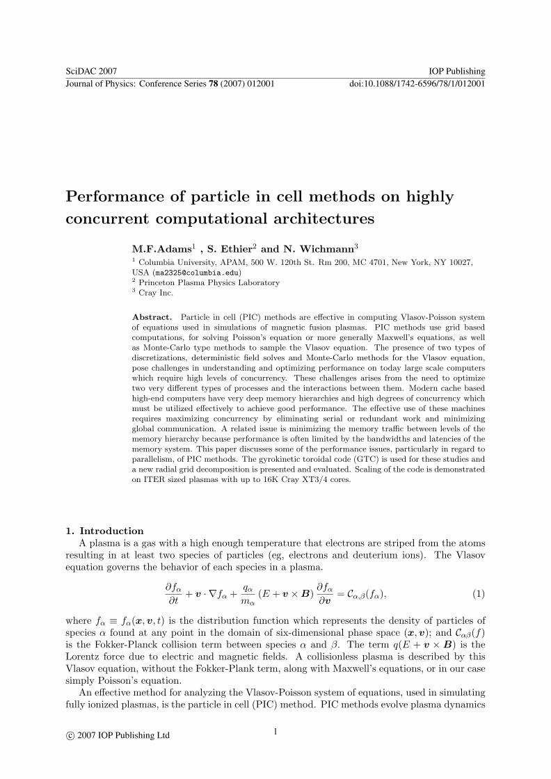
2. Gyrokinetic PIC algorithmThe basic PIC algorithm consists of depositing the charge from the particles onto the grid,

computing and smoothing the potential, computing the electric field and pushing particles withthe Lorentz force. Figure 1 shows a schematic of the PIC algorithm.

Performance is governed by three basic types of operations in this algorithm: 1) grids work(ie, Poisson solve), 2) particle processing (eg, position and velocity updates and 3) interpolationbetween the two (ie, charge deposition and field calculation in particle pushing). The dominantcomputational cost depends on the number of particles use; for the δf methods [5], used inGTC the grid work is a significant minority of the overall cost of the simulation, the cost beingdominated by particle pushing. Earlier version of GTC parallelized the grid work with a sharedmemory model (Open MP) which is adequate if the grid is small enough and the size of theshared address space for each poloidal plane is large enough. As devices get larger, and finergrids are desired for some types of simulations, performance degrades with this model becausemore address spaces are required for each plane and the larger grid that needs to be stored putsmore pressure on the cache and the entire memory system. This performance degradation isdue to increased pressure on the cache in the charge deposition and redundant work required


2

(x,v)← Initialize – Initialize (ion) particle position and velocitytime loop t = 1 : δt : T

¯δni ← Charge (x, q) – Deposit ion charge (q) on gridΦ← (

1−∇2⊥

)−1 ¯δni – Potential solve (small parameter expansion)Φ← Smooth (Φ) – Smooth potentialE ← ∇Φ – Compute electric field on gridv ← v + δt · qE/m – Update velocity (interpolate E from grid)x← x + δt · v – Update ion position

end loop

Figure 1. Schematic of the PIC algorithm

in the solve, field calculation and smoothing phases. The large fusion devices that now need tobe modeled and the small amount of shared memory parallelism available on the newest largemachines (ie, Cray XT4 and IBM Blue Gene have essentially no shared memory) requires adomain decomposition of the grid with MPI parallelism. This report discusses an MPI paralleldecomposition method for the grids in GTC.

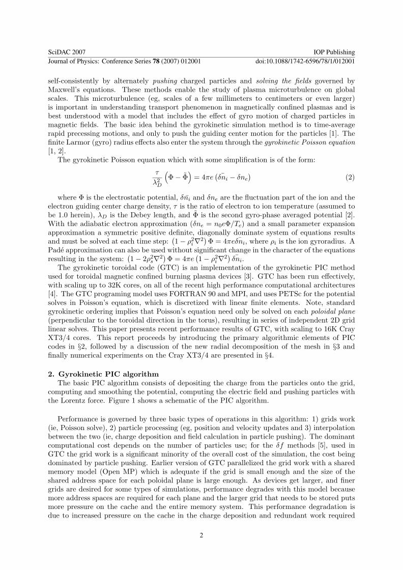
3. GTC mesh and decompositionFigure 2 (left) shows a diagram of a typical magnetic fusion tokamak device. GTC simulates

the core plasma; this is a toroidal domain with magnetic field lines with strong components inthe toroidal direction but with some component in the poloidal plane resulting in a “twisting”magnetic field. GTC generates meshes for poloidal planes where Poisson’s equation is solved.Thus, charge deposition first interpolates a particles charge to the two planes on each side of thetoroidal domain in which it is located. This charge on the poloidal plane is then interpolatedonto the mesh points. Figure 2 (center) shows a sample set of poloidal mesh points on a poloidalplane. Figure 2 (right) shows a sample global grid with the field line following grid lines. These

Figure 2. Fusion tokamak design schematic (left), GTC discretization of toroidal domain (right)

planes form a natural 1D decomposition of the computational domain, which is the primarydecomposition in GTC. The next section describes a new (radial) decomposition of the particles


3

and grid. This significantly complicates the parallel model in that the grid on the poloidal planemust be decomposed with explicit MPI parallelism.

3.1. Radial grid decompositionThe optimal grid decomposition for GTC is not obvious in that several efficiencies are

impacted by the decomposition in different ways. Additionally, the optimal method may bemore complex to implement than is necessary for acceptable performance in the range of devicesizes (up to 10K radial grid cells) and the computers of interest in the next several years (say640K cores and 128 poloidal planes, resulting in 4K processes per plane). The first thing tonote is that the particles move primarily along the magnetic field lines and thus do not movemuch in the radial direction. Thus, a radial partitioning will result in minimal communicationof particles within the poloidal plane. A fully 2D grid decomposition has the advantage that thesame decomposition can be used for the Poisson solver – currently a separate unstructured 2Ddecomposition is used. Also a structured 2D decomposition is not as efficient for the solver as anunstructured one when large amounts of parallelism are required. Given these trade-offs and therelative simplicity in implementation we have opted for a structure radial grid decomposition(1D in the plane) for the grid/particle computations and a 2D unstructured decomposition formost of the grid computations (ie, the Poisson solver).

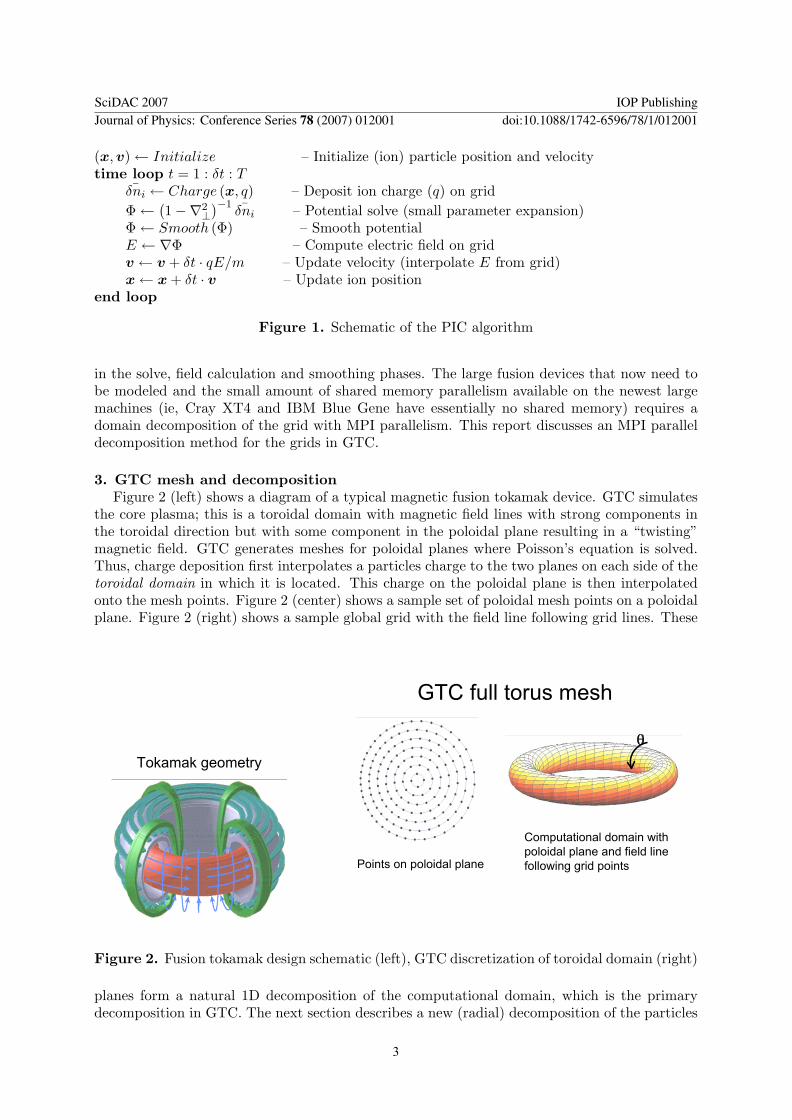
Our approach is to assume that the density of particles is a known function of radius (eg,a constant) and to compute a non-overlapping decomposition of the domain (ie, a geometricpartitioning) that balances the particles exactly (given the assumed distribution). Figure 3shows a small GTC grid of one plane (left) and a schematic of a geometric partitioning withfour radial domains (processors or cores). Note, the GTC computational domain has an innerhole of radius “a0” and an outer radius “a1” in Figure 3. The local domain, that needs to be

−1 −0.5 0 0.5 1

x

−1

−0.5

0

0.5

1

y

(a)

R(P)=R(1)

a0=R(0)

(b) geometric nonoverlapped partitioning

a1=R(P+4)=R(4=NP)

R(P+2)=R(3)

R(P+1)=R(2)

Figure 3. Sample GTC mesh (left), schematic if non-overlapping geometric radial partitioning(right)

stored on each processor, must be extended to accommodate the charge deposition. The particleposition stored in the gyrokinetic method is the guiding center of the particle – the gyrokineticformulation models the gyro motion as a charged ring around particles guiding center. Thischarged ring is discretized with a few points (eg, four) on the ring; the charge at these pointsis deposited on the grid with linear or bilinear interpolation. A small but trivial optimization


4

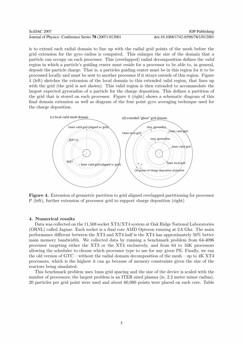
is to extend each radial domain to line up with the radial grid points of the mesh before thegrid extension for the gyro radius is computed. This enlarges the size of the domain that aparticle can occupy on each processor. This (overlapped) radial decomposition defines the validregion in which a particle’s guiding center must reside for a processor to be able to, in general,deposit the particle charge. That is, a particles guiding center must be in this region for it to beprocessed locally and must be sent to another processor if it strays outside of this region. Figure4 (left) sketches the extension of the local domain to this extended valid region, that lines upwith the grid (the grid is not shown). This valid region is then extended to accommodate thelargest expected gyroradius of a particle for the charge deposition. This defines a partition ofthe grid that is stored on each processor. Figure 4 (right) shows a schematic diagram of thisfinal domain extension as well as diagram of the four point gyro averaging technique used forthe charge deposition.

Inner valid grid (aligned w/ grid)

(c) local valid mesh domain

R(P+1)

R(P)

Outer valid grid (aligned w/ grid)

(4) points of charge deposition of particle

Inner valid grid

(d) extended "ghost" grid domain

max. gyroradius

max. gyroradius

Outer local gridOuter valid grid

Inner local grid

Figure 4. Extension of geometric partition to grid aligned overlapped partitioning for processorP (left), further extension of processor grid to support charge deposition (right)

4. Numerical resultsData was collected on the 11,508 socket XT3/XT4 system at Oak Ridge National Laboratories

(ORNL) called Jaguar. Each socket is a dual core AMD Opteron running at 2.6 Ghz. The mainperformance different between the XT3 and XT4 half is the XT4 has approximately 50% bettermain memory bandwidth. We collected data by running a benchmark problem from 64-4096processor targeting either the XT3 or the XT4 exclusively, and from 64 to 16K processorsallowing the scheduler to choose which processor type to use for any given PE. Finally, we ranthe old version of GTC – without the radial domain decomposition of the mesh – up to 4K XT3processors, which is the highest it can go because of memory constraints given the size of thereactors being simulated.

This benchmark problem uses 1mm grid spacing and the size of the device is scaled with thenumber of processors; the largest problem is an ITER sized plasma (ie, 2.2 meter minor radius).20 particles per grid point were used and about 60,000 points were placed on each core. Table


5

1 shows the parameters for the scaling study.

Case 1 2 3 4 5num. poloidal planes 64 64 64 64 64num. θ (max) 625 1,250 2,500 5,000 10,000num. radial points 100 200 400 800 1,600major radius (m) 0.388 0.775 1.55 3.1 6.2num. PEs 64 256 1,024 4,096 16,392

Table 1. Weak scaling benchmark GTC parameters

The minor radius is 0.32 times the major radius, the number of radial grid points and gridpoints in the θ direction are successively double. The plasma temperature is a constant at 2500for all cases.

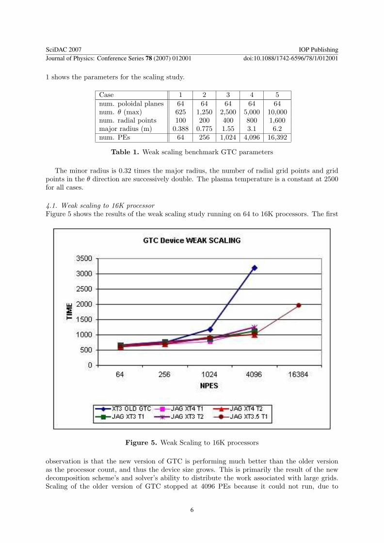
4.1. Weak scaling to 16K processorFigure 5 shows the results of the weak scaling study running on 64 to 16K processors. The first

Figure 5. Weak Scaling to 16K processors

observation is that the new version of GTC is performing much better than the older versionas the processor count, and thus the device size grows. This is primarily the result of the newdecomposition scheme’s and solver’s ability to distribute the work associated with large grids.Scaling of the older version of GTC stopped at 4096 PEs because it could not run, due to


6

memory constraints, and ITER size device using 16K processors. Scaling to 4096 processors isgood, but not as good as hoped for. Time approximately doubles while ideally it would stayflat. There does not appear to be much difference between the XT3 and the XT4, an earlyindication that the majority of the code is not sensitive to memory bandwidth. Moving to 16KPEs time almost doubles again. While a tremendous amount of science can be accomplished atthis number of PEs, the performance degrades significantly.

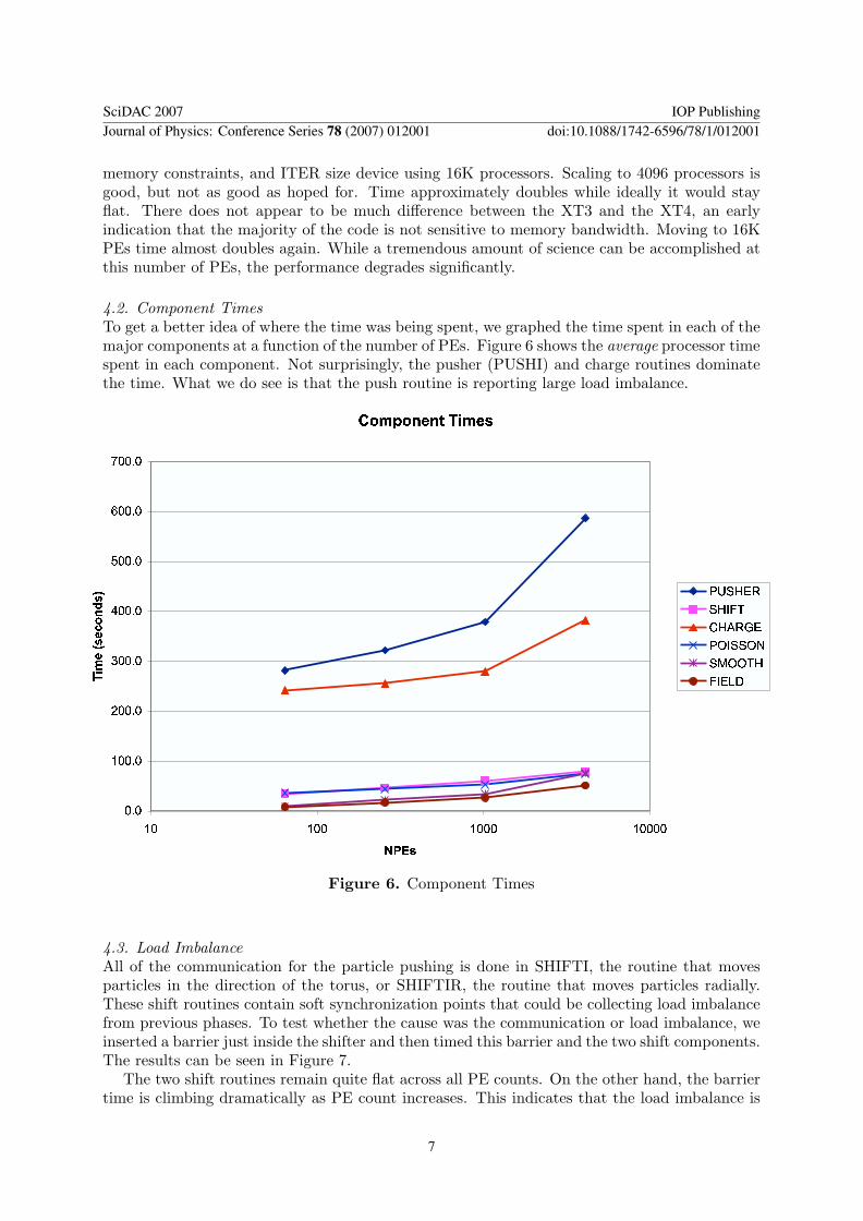
4.2. Component TimesTo get a better idea of where the time was being spent, we graphed the time spent in each of themajor components at a function of the number of PEs. Figure 6 shows the average processor timespent in each component. Not surprisingly, the pusher (PUSHI) and charge routines dominatethe time. What we do see is that the push routine is reporting large load imbalance.

Figure 6. Component Times

4.3. Load ImbalanceAll of the communication for the particle pushing is done in SHIFTI, the routine that movesparticles in the direction of the torus, or SHIFTIR, the routine that moves particles radially.These shift routines contain soft synchronization points that could be collecting load imbalancefrom previous phases. To test whether the cause was the communication or load imbalance, weinserted a barrier just inside the shifter and then timed this barrier and the two shift components.The results can be seen in Figure 7.

The two shift routines remain quite flat across all PE counts. On the other hand, the barriertime is climbing dramatically as PE count increases. This indicates that the load imbalance is


7

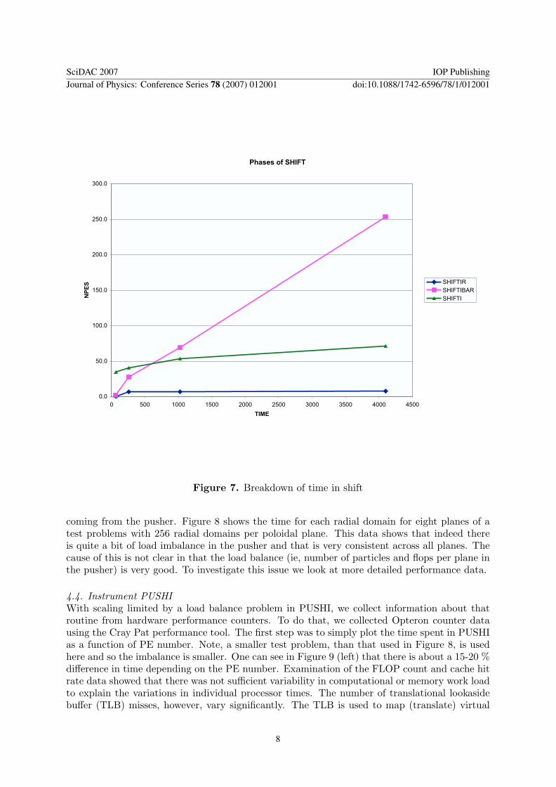
Phases of SHIFT

0.0

50.0

100.0

150.0

200.0

250.0

300.0

0 500 1000 1500 2000 2500 3000 3500 4000 4500

TIME

NP

ES SHIFTIR

SHIFTIBAR

SHIFTI

Figure 7. Breakdown of time in shift

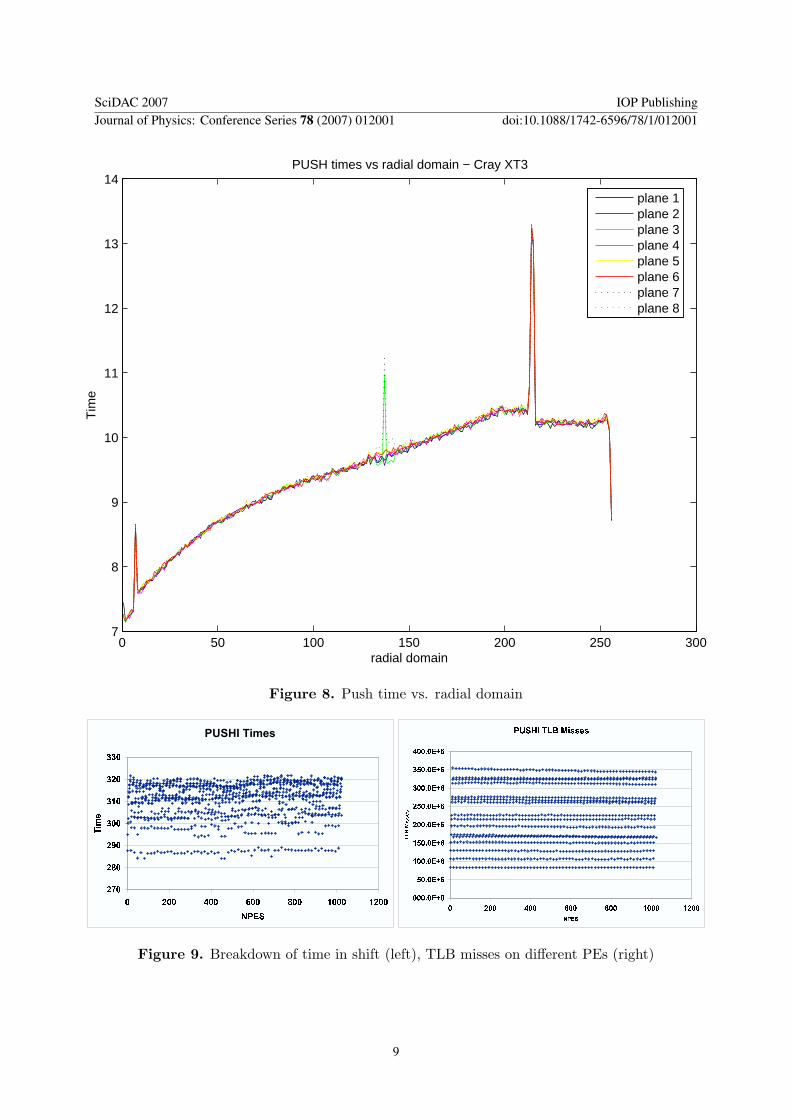
coming from the pusher. Figure 8 shows the time for each radial domain for eight planes of atest problems with 256 radial domains per poloidal plane. This data shows that indeed thereis quite a bit of load imbalance in the pusher and that is very consistent across all planes. Thecause of this is not clear in that the load balance (ie, number of particles and flops per plane inthe pusher) is very good. To investigate this issue we look at more detailed performance data.

4.4. Instrument PUSHIWith scaling limited by a load balance problem in PUSHI, we collect information about thatroutine from hardware performance counters. To do that, we collected Opteron counter datausing the Cray Pat performance tool. The first step was to simply plot the time spent in PUSHIas a function of PE number. Note, a smaller test problem, than that used in Figure 8, is usedhere and so the imbalance is smaller. One can see in Figure 9 (left) that there is about a 15-20 %difference in time depending on the PE number. Examination of the FLOP count and cache hitrate data showed that there was not sufficient variability in computational or memory work loadto explain the variations in individual processor times. The number of translational lookasidebuffer (TLB) misses, however, vary significantly. The TLB is used to map (translate) virtual


8

0 50 100 150 200 250 3007

8

9

10

11

12

13

14

radial domain

Tim

e

PUSH times vs radial domain − Cray XT3

plane 1plane 2plane 3plane 4plane 5plane 6plane 7plane 8

Figure 8. Push time vs. radial domain

Figure 9. Breakdown of time in shift (left), TLB misses on different PEs (right)


9

address to physical memory addresses and is similar to the memory cache in some respects (eg,there are many levels of TLBs and if an address is not found than an expensive “page fault”occurs).

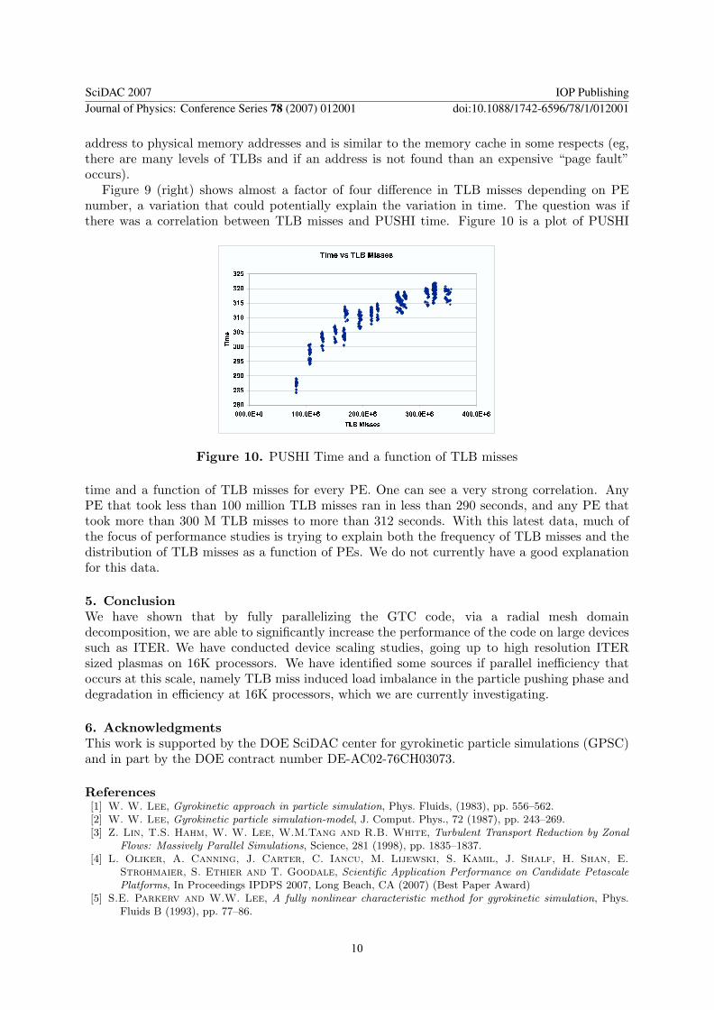
Figure 9 (right) shows almost a factor of four difference in TLB misses depending on PEnumber, a variation that could potentially explain the variation in time. The question was ifthere was a correlation between TLB misses and PUSHI time. Figure 10 is a plot of PUSHI

Figure 10. PUSHI Time and a function of TLB misses

time and a function of TLB misses for every PE. One can see a very strong correlation. AnyPE that took less than 100 million TLB misses ran in less than 290 seconds, and any PE thattook more than 300 M TLB misses to more than 312 seconds. With this latest data, much ofthe focus of performance studies is trying to explain both the frequency of TLB misses and thedistribution of TLB misses as a function of PEs. We do not currently have a good explanationfor this data.

5. ConclusionWe have shown that by fully parallelizing the GTC code, via a radial mesh domaindecomposition, we are able to significantly increase the performance of the code on large devicessuch as ITER. We have conducted device scaling studies, going up to high resolution ITERsized plasmas on 16K processors. We have identified some sources if parallel inefficiency thatoccurs at this scale, namely TLB miss induced load imbalance in the particle pushing phase anddegradation in efficiency at 16K processors, which we are currently investigating.

6. AcknowledgmentsThis work is supported by the DOE SciDAC center for gyrokinetic particle simulations (GPSC)and in part by the DOE contract number DE-AC02-76CH03073.

References[1] W. W. Lee, Gyrokinetic approach in particle simulation, Phys. Fluids, (1983), pp. 556–562.[2] W. W. Lee, Gyrokinetic particle simulation-model, J. Comput. Phys., 72 (1987), pp. 243–269.[3] Z. Lin, T.S. Hahm, W. W. Lee, W.M.Tang and R.B. White, Turbulent Transport Reduction by Zonal

Flows: Massively Parallel Simulations, Science, 281 (1998), pp. 1835–1837.[4] L. Oliker, A. Canning, J. Carter, C. Iancu, M. Lijewski, S. Kamil, J. Shalf, H. Shan, E.

Strohmaier, S. Ethier and T. Goodale, Scientific Application Performance on Candidate PetascalePlatforms, In Proceedings IPDPS 2007, Long Beach, CA (2007) (Best Paper Award)

[5] S.E. Parkerv and W.W. Lee, A fully nonlinear characteristic method for gyrokinetic simulation, Phys.Fluids B (1993), pp. 77–86.


10

Performance of particle in cell methods on highly ...

Documents

Transcript of Performance of particle in cell methods on highly ...