Graduate Theses, Dissertations, and Problem Reports

2016

Performance Improvement Study on High Horsepower Performance Improvement Study on High Horsepower

Compression Ignition Diesel Engines in Mining Haul Trucks at Compression Ignition Diesel Engines in Mining Haul Trucks at

High Altitude High Altitude

Michael S. Wise

Follow this and additional works at: https://researchrepository.wvu.edu/etd

Recommended Citation Recommended Citation Wise, Michael S., "Performance Improvement Study on High Horsepower Compression Ignition Diesel Engines in Mining Haul Trucks at High Altitude" (2016). Graduate Theses, Dissertations, and Problem Reports. 6962. https://researchrepository.wvu.edu/etd/6962

This Thesis is protected by copyright and/or related rights. It has been brought to you by the The Research Repository @ WVU with permission from the rights-holder(s). You are free to use this Thesis in any way that is permitted by the copyright and related rights legislation that applies to your use. For other uses you must obtain permission from the rights-holder(s) directly, unless additional rights are indicated by a Creative Commons license in the record and/ or on the work itself. This Thesis has been accepted for inclusion in WVU Graduate Theses, Dissertations, and Problem Reports collection by an authorized administrator of The Research Repository @ WVU. For more information, please contact researchrepository@mail.wvu.edu.

Performance Improvement Study on High Horsepower Compression Ignition Diesel

Engines in Mining Haul Trucks at High Altitude

Michael S. Wise

Thesis submitted to the

Benjamin M. Statler College of Engineering

and Mineral Resource at West Virginia University

in partial fulfillment of the requirements for the degree of

Master of Science in

Mechanical Engineering

Dr. Gregory Thompson, Chair

Dr. Arvind Thiruvengadam

Dr. Hailin Li

Department of Mechanical Engineering

Morgantown, West Virginia

2016

Keywords: [Diesel Engines, High Horse Power, Performance, Combustion, High Altitude]

Copyright 2016 Michael S. Wise

Abstract Performance Improvement Study on High Horsepower Compression Ignition Diesel

Engines in Mining Haul Trucks at High Altitude

Michael S. Wise

Railways and mining operations are reaching new heights as end users break altitude

barriers to increase efficiencies of their business and provide more goods. Diesel engines are the

primary source of power used in both of these applications, whether it is for electricity

generation or transportation of products. In particular, the copper and gold mining occurring in

the Andes Mountains require diesel engines to operate at altitudes above 15,000 ft. At these

altitudes the air density is low and the air temperature often falls below 0° F during the winter,

providing a less than ideal atmosphere for the operation of a diesel engine. However, end users

are demanding improved performance, fuel economy, and reliability as part of their push to

optimize production and minimize costs.

As part of this effort to improve operation of diesel engines at high altitudes, engine

manufacturers like Cummins are tailoring calibrations to oblige the customer. After making

calibration modifications, a field test was conducted on a Komatsu 930E haul truck with a GE

electric drive train at approximately 16,000 ft to assess the in-cylinder combustion events and

compare them to an engine operating near 500 ft in a test cell.

Idiosyncrasies were identified for the Cummins QSK 60L engine incorporating a HPI

fuel system. It was observed that the first cylinder on each bank was found to underperform

when compared to the other instrumented cylinders. With respect to the maximum in-cylinder

pressure, the greatest amount of cylinder-to-cylinder variation was witnessed during dynamic

braking for both test; 4% during the test cell work and 12.97 % during the field test. The least

amount of variation was witnessed during rated operation at 0.59 % and 0.22 % for the test cell

data and field test data respectively. The calibration changes made by Cummins resulted in

virtually no distinguishable differences in combustion while the engine was operating at rated

conditions. The largest differences in combustion were observed during dynamic braking and

dumping operating modes. The peak in-cylinder pressures were found to be approximately 26 %

lower, on average, for both modes of operation at high altitudes. The most significant impact

found on the combustion process from altitude effects was increased ignition delays. A linear

correlation was found during the dumping operation that showed increased ignition delays which

resulted in higher maximum heat release rates. The maximum heat release rate was found to

increase approximately 41.47 %, on average, between the test cell data and the field test data.

Despite a 26 % decrease in the maximum in-cylinder pressure observed during the field tests, the

final heat release exhibited by each engine remained within 10 %. Improved thermal efficiencies

were observed at high altitude compared to sea level for the low load operating points at 2 % and

11 %, on average, for the dumping mode and dynamic braking mode respectively which was

consistent with the reduce PMEP values at altitude.

iii

Acknowledgments I would like to begin by thanking my fiancé Cassandra. She has been my rock throughout my

entire engineering career giving me love and praise through very hard times. Despite my choices

to spend countless late nights at the engine lab and living in another state for an entire year to

further my career she has stuck by my side always encouraging me to do what is right.

I would like to thank all of my CAFEE brothers. There are many, so to speak to the masses, you

have all bettered me as a person in one way or another. Whether it was a late night in the ERC or

a late night beer and hot wings, you have all made my time at WVU unforgettable.

I would like to thank Ross Ryskamp for being like a big brother and helping me build my

confidence through the years. You have taught me fabrication, engineering, and how to be a

mechanic. I believe I have molded my engineering judgment skills and work ethic by working

under you which I attribute much of my success to.

I would like to thank Dan Carder for making me a part of CAFEE and pushing me outside of my

comfort zone. You have taught me to take ownership in all that I do and that failure is not an

option. You have been a wonderful role model and I very much hope to be and engineer and

leader of the caliber that you are.

I would like to thank Dr. Greg Thompson for taking a risk on a student with low confidence. I

initially had hoped he would be my adviser because I thought he would be hard on me and force

me to become a better engineer and student. Dr. Thompson has a way of demanding excellence

without asserting force and as a result I was never forced to do anything but made leaps and

bounds in my maturity as an individual as well as an engineer. He has made an effort to connect

with me outside of work and school which he will never know how grateful that I am for that.

iv

You have taught me the value in what it means to struggle rather than just getting the fastest

answer as well as how to look past all of the small problems to see a functional system.

I would like to thank Duane Kruer for being and excellent boss and role model during my time

with Cummins. You have encouraged me to take on several high priority projects and have

helped me see them through to completion. By working with you I have learned how to handle

sensitive matters with finesse and to look past peoples imperfections to see their valuable

contribution. You have taught me to take risks and get the most out of people. You are a great

leader and I feel fortunate to have worked under you. Lastly, I would like to thank you for

pushing the Cummins sponsorship of my thesis. Without that, I would not have been able to

finish my degree.

I would like to thank Dr. Arvind Thiruvengadam for introducing me to CAFEE. If it were not for

you I would not have been exposed to the world of engine testing which is what I have come to

love. Your positive attitude and determination is infectious making me enjoy every moment

spent with you. I have looked up to you since day one and hope to follow in your footsteps.

I would to thank Dr. Marc Besch for giving me his time and patients throughout the years to

answer my questions. Known for notoriously being over worked, you have always spared time to

further my understanding. I can honestly say I have never walked away from a conversation with

you without knowing more than when I showed up.

I would like to thank Cummins and all of those who have contributed to my thesis.

v

Table of Contents Abstract ........................................................................................................................................... ii

Acknowledgments.......................................................................................................................... iii

Table of Contents ............................................................................................................................ v

Table of Figures ........................................................................................................................... viii

List of Tables .................................................................................................................................. x

1.0 Introduction ............................................................................................................................... 1

1.1 Overview ............................................................................................................................... 1

1.2 Objective ............................................................................................................................... 3

2.0 Literature Review...................................................................................................................... 5

2.1 Fuel Properties ...................................................................................................................... 5

2.1.1 Density and Specific Gravity ......................................................................................... 7

2.1.2 Cetane ............................................................................................................................ 7

2.1.3 Aromatics ....................................................................................................................... 7

2.1.4 Heating Value ................................................................................................................ 8

2.1.5 Volatility ........................................................................................................................ 8

2.1.6 Other Properties ............................................................................................................. 9

2.2 Combustion Analysis ............................................................................................................ 9

2.2.1 In-Cylinder Pressure Measurement................................................................................ 9

2.2.2 Single Zone Analysis ................................................................................................... 11

2.2.3 Heat Release................................................................................................................. 14

2.3 Diesel Combustion .............................................................................................................. 14

2.3.1 Injection Characteristics............................................................................................... 15

2.3.2 Injection Timing........................................................................................................... 17

2.3.3 Turbocharging .............................................................................................................. 19

2.3.4 Effects of Atmospheric Conditions .............................................................................. 20

2.3.5 Combustion Variation and Fluctuations ...................................................................... 23

3.0 Experimental Setup ................................................................................................................. 25

3.1 Introduction ......................................................................................................................... 25

3.2 Differences in Performance Hardware ................................................................................ 25

3.3 Field Data Collection .......................................................................................................... 26

3.3.1 Test Cycle .................................................................................................................... 26

vi

3.3.2 In-Cylinder HSDA System .......................................................................................... 30

3.3.3 Cylinder Pressure ......................................................................................................... 32

3.3.4 Trigger and Speed ........................................................................................................ 32

3.3.5 Injection ....................................................................................................................... 33

3.3.6 IMP .............................................................................................................................. 33

3.3.7 IMEP ............................................................................................................................ 34

3.3.8 HRR ............................................................................................................................. 34

3.3.9 Thermal Efficiency ...................................................................................................... 35

3.3.10 Heat Release............................................................................................................... 35

3.3.11 Mass Fraction Burned ................................................................................................ 35

3.3.12 Ignition Delay ............................................................................................................ 36

3.3.13 Maximum In-Cylinder Pressure ................................................................................. 36

3.4 Test Cell Data Collection .................................................................................................... 36

3.4.1 Test Cell Hardware/ Instrumentation ........................................................................... 36

3.4.2 In-Cylinder HSDA System .......................................................................................... 37

3.4.3 Test Condition .............................................................................................................. 39

3.4.4 Test Cycle .................................................................................................................... 39

4.0 Results and Discussion ........................................................................................................... 41

4.1 Introduction ......................................................................................................................... 41

4.2 Test Cell Data Reduction .................................................................................................... 41

4.2.1 Rated Operation Pressure Analysis .............................................................................. 41

4.2.2 Dumping Operation Pressure Analysis ........................................................................ 45

4.2.3 Dynamic Braking Operation Pressure Analysis .......................................................... 50

4.3 In-Field Data Reduction ...................................................................................................... 55

4.3.1 Rated Mode of Operation Pressure Analysis ............................................................... 55

4.3.2 Dumping Mode of Operation Pressure Analysis ......................................................... 60

4.3.3 Dynamic Braking Mode of Operation Pressure Analysis ............................................ 64

4.4 Evaluation of Altitude ......................................................................................................... 69

4.4.1 Rated Mode of Operation Comparison ........................................................................ 69

4.4.2 Dumping Mode of Operation Comparison .................................................................. 74

4.4.3 Dynamic Braking Mode of Operation Comparison ..................................................... 80

5.0 Conclusions ............................................................................................................................. 87

vii

6.0 Recommendations ................................................................................................................... 90

7.0 References ............................................................................................................................... 91

8.0 Appendices .............................................................................................................................. 93

8.1 Commanded and Measured Operating Parameters ............................................................. 93

8.2 Rocker Strain Gage Signal for HPI Injector ....................................................................... 93

8.2 Ready Mode Operation Pressure Analysis Curves (Test Cell) ........................................... 94

8.3 Field Test Fuel Analysis ..................................................................................................... 95

viii

Table of Figures Figure 1 Dynamic in-cylinder pressure curve at low load and speed operating conditions. ........ 10

Figure 2 Representative HRR at 1200rpm and 1500ft-lb torque. ................................................. 13

Figure 3 Representative normalized heat release curve. ............................................................... 14

Figure 4 Cummins HPI fuel injector [Cummins HHP-HPI Fuel System Training Presentation]. 16

Figure 5 Representative compressor map [Cummins Holset]. ..................................................... 20

Figure 6 Compressor maps for both turbochargers tested in the test cell [Cummins Holset: FAE

Maps]. ........................................................................................................................................... 26

Figure 7 Duty cycle of a haul truck at the Caserones mine. ......................................................... 28

Figure 8 Torque curve from test cell compared to the GE loading curve in a haul truck. ............ 29

Figure 9 AVL INDIMICRO™ unit with an AVL Vehicle Interface module used during field

testing. ........................................................................................................................................... 31

Figure 10 Pressure curves for cylinders 1 left and 8 right at rated conditions.............................. 42

Figure 11 HRR curve for cylinders 1 left and 8 right at rated operating conditions. ................... 43

Figure 12 Heat release curve for rated operating conditions for cylinder 1 left and 8 right. ........ 44

Figure 13 Pressure curve for a simulated dumping mode of operation. ....................................... 46

Figure 14 HRR curve for dumping mode of operation. ................................................................ 47

Figure 15 Heat release curve for dumping mode of operation. .................................................... 49

Figure 16 shows the pressure curves for the dynamic braking operating mode. .......................... 50

Figure 17 shows the HRR curve for the dynamic braking mode of operation. ............................ 52

Figure 18 shows the heat release curve for the dynamic braking mode of operation. .................. 53

Figure 19 Pressure curve for rated mode of operation. ................................................................. 55

Figure 20 HRR curve for rated mode of operation. ...................................................................... 57

Figure 21 Heat release for rated operating condition.................................................................... 58

Figure 22 Pressure curve for dumping mode of operation. .......................................................... 60

Figure 23 HRR for dumping mode of operation. .......................................................................... 62

Figure 24 Heat release curve for dumping mode of operation. .................................................... 63

Figure 25 Pressure curve for dynamic braking operation. ............................................................ 65

Figure 26 HRR for dynamic braking mode of operation. ............................................................. 66

Figure 27 HRR for dynamic braking mode of operation. ............................................................. 68

Figure 28 Pressure curve for rated operating conditions for both tests. ....................................... 70

Figure 29 HRR curve for rated mode of operation for both test conducted. ................................ 71

Figure 30 Heat release curve for rated mode of operation. ........................................................... 73

Figure 31 Pressure curve for dumping mode of operation. .......................................................... 74

Figure 32 HRR for dumping mode of operation. .......................................................................... 76

Figure 33 Correlation of ignition delay to maximum HRR for dumping mode of operation. ...... 78

Figure 34 HRR curves for dumping mode of operation. .............................................................. 78

Figure 35 Pressure curves for dynamic braking mode of operation. ............................................ 80

Figure 36 HRR curves for dynamic braking mode of operation. ................................................. 82

Figure 37 Maximum HRR relation to ignition delay. ................................................................... 83

Figure 38 Heat release for dynamic braking mode of operation. ................................................. 84

Figure 39 Rocker strain gage curve for dynamic braking (Commanded timing 10°BTDC) ........ 93

ix

Figure 40 Pressure curve for ready mode operation ..................................................................... 94

Figure 41 HRR curve for ready mode operation .......................................................................... 94

Figure 42 Heat release curve for ready mode operation ............................................................... 94

x

List of Tables Table 1 Key fuel properties and limits that are regulated by the governing bodies in Chile and the

USA for non-road diesel [ASTM D975, dieselnet.com]. ............................................................... 6

Table 2 shows the time spent at each operating mode for a haul truck in a pit mine. .................. 30

Table 3 shows the steady state operating conditions chosen to evaluate for this effort. .............. 41

Table 4 Provides pertinent information derived from the pressure curve for the rated mode of

operation. ...................................................................................................................................... 43

Table 5 Maximum HRR and location. .......................................................................................... 44

Table 6 MFB results for rated operating conditions. .................................................................... 45

Table 7 Maximum cylinder pressure and pertinent information derived from the pressure curve

for the dumping mode of operation. ............................................................................................. 46

Table 8 Maximum HRR and subsequent information derived from the HRR curve for dumping

mode of operation. ........................................................................................................................ 48

Table 9 Location of MFB for the dumping mode of operation. ................................................... 49

Table 10 Maximum in-cylinder pressures and pertinent information derived from the pressure

curve for dynamic braking mode of operation. ............................................................................. 51

Table 11 Maximum HRR, the location of maximum HRR, and ignition delay for dynamic

braking mode of operation. ........................................................................................................... 52

Table 12 MFB results for dynamic braking operating conditions. ............................................... 54

Table 13 Maximum pressure and pertinent information derived from the pressure curve. .......... 56

Table 14 Maximum HRR, location of maximum HRR, and ignition delay. ................................ 57

Table 15 MFB results for rated operation. .................................................................................... 59

Table 16 Maximum pressure and derived information from the pressure curve for rated mode of

operation. ...................................................................................................................................... 61

Table 17 Maximum HRR, location of maximum HRR, and ignition delays for dumping mode of

operation. ...................................................................................................................................... 62

Table 18 MFB assessment for the dumping mode of operation. .................................................. 64

Table 19 Maximum in-cylinder pressure and pertinent information derived from the pressure

curve for dynamic braking mode of operation. ............................................................................. 66

Table 20 Maximum HRR, location of maximum HRR, and ignition delays for dynamic braking

mode of operation. ........................................................................................................................ 67

Table 21 MFB assessment for dynamic braking mode of operation. ........................................... 69

Table 22 Diffusion combustion burn rate by MFB assessment. ................................................... 79

Table 23 Crank angle differences between respective MFB locations. ........................................ 85

Table 24 Commanded parameters and measured operating conditions for all runs. .................... 93

1

1.0 Introduction

1.1 Overview

There is a growing need for higher altitude capabilities from engine manufacturers as

railroads are reaching new heights throughout the world and the copper mining in the Chilean

Mountains tries to keep up with market demand [Ebert and Menza, 2015]. In 2004, the Qinghai-

Tibet railway was completed making it the highest altitude railway in the world at 16,640 ft

[Dingding, 2006]. The mining occurring in the Andes Mountains around 15,000 ft are requiring

haul trucks to operate not only at high altitudes but within temperature ranges of -40° F to 131° F

and under continuous operation [Koellner, 2004].

The ambient conditions at high altitude are the primary reason that engines do not operate

well. The air pressure, and hence density, is inversely proportional to altitude. Turbocharging

helps counter issues with low ambient air density and pressure by compressing the air, but this is

only beneficial once the compressor wheel reaches an effective speed while transitioning from

low power (such as idle) to high power. In order for the compressor to increase the speed, the

engine needs to react independently of the turbocharger to transition to a speed when the

turbocharger is effective. It is during this period that fuel must be strategically injected with the

proper amount and at the right time in order for the compressor wheel to reach effective speeds

without causing the engine harm.

Engines will experience lower peak in-cylinder pressures at high altitudes because of

reduced air densities. Several studies have noted that engines that operate in high altitudes with

an injection timing developed for sea level operation experience longer ignition delays and

reduced thermal efficiency [Wang et. al., 2013]. Reduced efficiencies at high altitude were also

pointed out by Ferguson and Kirkpatrick when observing the ratio of BMEP (brake mean

2

effective pressure) at sea level and at high altitudes [Ferguson and Kirkpatrick, 2001]. The

combustion in an engine represents the collaboration of almost every system in the engine. For

this application those of greater importance are the air handling and the fuel injection system.

The air handling system determines how much fuel can be injected based on how much oxygen

is available to react and the fuel system determines at what time and duration the fuel can be

injected to begin reacting. Both of these have a great effect on the performance of the engine and

efficiency of the energy conversion of the liquid fuel from chemical energy to mechanical

energy. To better understand these relationships, in-cylinder pressure analysis has been

developed over the years using different theoretical approaches. One approach is a single-zone

analysis that is highlighted in Heywood [Heywood, 1988]. This analysis is based on a single

moving pressure wave that propagates the length of the cylinder propelling the piston downward.

From this analysis, fuel conversion efficiencies can be inferred, the ignition properties of the fuel

can be evaluated regarding ignition delays and burn rates, and mechanical limits can be set based

on the in-cylinder pressures. The basis of this analysis begins with an in-cylinder pressure

measurement achieved with a piezoelectric pressure transducer and a HSDA (high speed data

acquisition) system. It is from this signal that most of the information listed above is derived.

Along with the in-cylinder pressure signal, the injection signal is utilized in determining the

ignition delay and the injection duration. This information is collected alongside the in-cylinder

pressure signal with the HSDA system. The measuring device can include strain gage mounted

to the rocker lever engaging the mechanical style injector or a current clamp attached to the

electronic style injector. Most electronic injectors produce a square wave-like signal to indicate if

it is injecting or not injecting but the mechanical injectors using a strain gage can reveal the

3

dynamics of the injector. The analysis in this thesis will be focused on an in-cylinder pressure

signal.

End users are reaching out to the engine manufacturers demanding improved fuel economy

and performance to help reduce fuel cost and improve productivity at high altitudes. To improve

fuel economy, the engine needs to operate more efficiently; to increase productivity, better

engine transient responses and increased power are required. Both of these demands are difficult

to achieve at the same time let alone at high altitudes. Companies like Cummins are taking on the

challenge by tailoring calibrations and new engine configurations to operate solely at high

altitude conditions. In tailoring the engine configurations, a wide range of performance parts

such as pistons, injectors, and turbochargers can be explored to best suit the customer

requirements while maintaining efficient operation. The engine calibrations have limited

adjustability since the high altitude customers typically buy older technology products because

they come at a reduced cost and are not emission regulated at such high altitudes. However, with

the Cummins HPI legacy fuel system, the quantity of fuel and amount of fuel can be controlled

within the mechanical ability of the system. Testing has been done to observe the effects on an

engine at sea level and altitude but none to the author’s knowledge have manipulated the engine

hardware or calibration [Wang et. al., 2013].

1.2 Objective

The objective of this work was to evaluate the operation of a Cummins QSK 60L CI

(compression ignition) diesel engine with a two-stage turbocharging system at sea level and at

altitudes close to 16,000 ft. Recent efforts have been made by Cummins to explore new

performance hardware and ECM calibration changes to increase thermal efficiency. The specific

changes in the engine hardware and control algorithms are not discussed in detail due to the

4

proprietary nature of the work. However, the evaluation of the in-cylinder combustion

characteristics after changes were made will be compared to the combustion observed near sea

level to identify significant disparities as part of an effort to improve high altitude combustion.

5

2.0 Literature Review Diesel engine designers, like all heat engine designers, must balance the thermodynamic

laws governing energy conversion with the manufacturing requirements. There are numerous

parameters that the designer has the ability to adjust to develop an engine including bore, stroke,

boost pressure level, and injection control strategy. However, once an engine has been designed,

there are a fixed amount of parameters (hardware or software) that can be controlled to change

how the engine operates. In order to quantify the effects of each change it is necessary to identify

experimental equipment, such as in-cylinder pressure measurements via piezoelectric pressure

transducers, to evaluate the engine’s performance. The following sections identify the major

variables that govern the engines operation and provide insight on how each variable can impact

engine performance through analysis.

2.1 Fuel Properties

Diesel fuel properties will be described in detail below in line of the focus of this work. It

should be noted that due to the lack of fuel property data, the properties of the fuel used for this

effort will not be discussed during the results of this paper. However, the significance of fuel

properties on the diesel combustion process is recognized and therefor necessary to highlight as

supporting material.

Diesel fuel is generally a distillate that comes from crude oil as it is the lowest cost

processing method. Other methods of production have been developed, such as Fischer-Tropsch

process, but are more costly compared to distillation refinery processes [Chevron, 2007]. In the

United States, the defining standard for determining diesel fuel properties is ASTM D975.

Similarly, the Ministerio de Energia in Chile has adopted many of the same ASTM standards to

define their limiting metrics for their diesel [ASTM D975, dieselnet.com]. Other countries such

6

as the United Kingdom have adopted their own standards, EN590, that consists of ISO

(international organization of standardization) standards [EN 590].

The differences in fuel properties from the country where an engine is developed and

where it operates can impact the combustion performance. Table 1, below shows the differences

in the diesel fuel property standards from three different countries the test engine operates in as

well as the fuel properties from a sample taken during the field test and in the test cell.

Table 1 Key fuel properties and limits that are regulated by the governing bodies in Chile and the USA for non-road diesel

[ASTM D975, dieselnet.com].

It can be seen that, relatively speaking, each country regulates their diesel to have

approximately the same property values with the exception of cetane number, Ramsbottom

carbon residue on 10 % distillation residue, and lubricity. Additionally, there are supplementary

properties like pour point that have different values. The reason for the difference between

regulated values arrives from the geographical and climatic difference from country to country.

USA,

No. 2-D S15

Chile,

Diesel B-1

UK,

EN 590:2004

Field Test

Sample

Test Cell

Sample

Property Limits Limits Limits Properties Properties

Flash Point, °C min 52 52 55 68 -

Water and Sediment, %vol

max0.05 0.05 0.02 - -

Distillation Temperature, °C

90% recovered282 - 338 282 - 338 360 max 338 - 636 -

Kinematic Viscosity, mm2/S

@40°C1.9 - 4.1 1.9 - 4.1 2.0 - 4.5 2.9 3.2

Ash % mass, max 0.01 0.01 0.01 - -

Sulfur, ppm (μg/g) max 15 15 10 13 -

Copper strip corrosion rating

3 h @ 50°CNo. 3 No. 1 Class 1 - -

Cetane number, min 40 50 51 54.3 -

Cetane Index, min 40 50 46 - -

Aromaticity, % vol, max 35 35 8 22.4 -

Ramsbottom carbon resideue

on 10% distillation residue,

% mass, max

0.35 0.21 0.3 - -

Lubricity, HFRR @ 60°C,

micron, max520 460 460 - -

Specific Gravity - .820 - .850 .845 max 0.8384 0.8375

7

Using Chile as an example, most of the country is either at high altitude due to the Andes

Mountain range or experience cold temperatures at the southern tip of the country do to its

proximity to the southern pole, thus the need for diesel with properties suitable for climates such

as these.

2.1.1 Density and Specific Gravity

The density and specific gravity of a fuel can influence how an engine will operate

pertaining to fuel economy and power output. The injection characteristics are often dependent

on the density of a fuel along with geometry of the injector itself. Fueling strategies are

dependent on the density of the fuel, along with many other variables, to meter the amount of

fuel being injected into the cylinder. Without an accurate approximation of the density, the

power output can vary.

2.1.2 Cetane

Cetane number is the defining characteristic of ignition quality for diesel. Defined by the

mixture of the reference fuels n-hexadecane and heptamethylnonane. The fuel n-hexadecane

represents the upper end of the cetane number and heptamethylnonane representing the lower

end of the cetane number [Heywood, 1988].

Having a higher Cetane number for diesel fuel is desirable to control the combustion

process more closely. A diesel fuel with lower cetane number results in longer ignition delays

resulting in large peak HRR (heat release rate) values and peak pressures [Heywood, 1988]. Due

to these undesirable effects, manufacturers assume a Cetane number that their customers will be

using in order to develop their calibrations.

2.1.3 Aromatics

Diesel fuel consists of many different hydrocarbon chains that are defined by the crude

oil source and the processes used to refine it. The hydrocarbon chains in diesel fuel can

8

determine the anti-knocking properties of a fuel as well as its combustion characteristics and

energy content. Aromatics, in particular, are hydrocarbon ring structures that are built from

benzene rings and can contain heavy alkyl groups on the sides. Due to its complex structure,

fuels containing a higher aromatic content are more difficult to break down making them prone

to knocking and require a higher flame temperature to initiate the dissociation process

[Heywood, 1988].

2.1.4 Heating Value

The heating value of a fuel is a non-regulated value that defines the amount of energy

contained within the fuel. Tests such as ASTM 240 and the more repeatable D4809 are

conducted with a bomb calorimeter where a hydrocarbon fuel is entered into a fixed volume

device and ignited while precise measurements for fuel mass and the resulting temperature rise

are recorded [ASTM D240, D4809]. From the temperature rise, the total heat from the

hydrocarbon fuel is determined. The heating value of a fuel is important when designing a heat

engine to ensure maximum reliability and optimized efficiency are achieved. It is for this reason

heat engines are most often designed to operate on one fuel so the heating value, among other

properties, remain within a specific range.

2.1.5 Volatility

Volatility is a term used to define a substance’s ability to evaporate. As a fuel property,

this is a critical parameter to consider when designing fuel injection system. Diesel fuel is

considered to have low volatility amongst hydrocarbon fuels and thus needs to be accounted for

to design the injection process. In a direct injection diesel engine the mixing of the fuel with the

fresh air charge relies heavily on the geometry and operating condition of the engine as well as

the fuel properties. During an injection event, a liquid length is established before the fuel begins

to vaporize and mix with the fresh air charge. The fuels volatility has a high correlation to the

9

liquid length developed during injection, as established by Canaan et al. [Canaan et al., 1998]. If

the liquid length is too long, the spray penetration will reach the cylinder walls causing fuel to

enter the oil system which can degrade the lubricating effects of oil. Subsequently, dilution of

lubrication oil with diesel fuel may lead to premature engine failure. Additionally, unburned fuel

will reduce the fuel conversion efficiency.

2.1.6 Other Properties

There are many additional properties of diesel fuel that are not covered in this effort due

to their relatively insignificant impact on combustion. Many fuel properties are interrelated and

can often be described in terms of another property such as volatility and boiling point or Cetane

and viscosity. Jeihouni et al. showed that many fuel properties provide high correlations between

one another, specifically, Cetane and aromatic content [Jeihouni et al. 2011]. Because of the lack

of fuel property data available from historical data used in this work, no additional commentary

will be made regarding fuel properties.

2.2 Combustion Analysis

There is a growing need for combustion analysis throughout the automotive industry for

creating combustion strategies and training computer models. Currently, evaluating in-cylinder

pressure data is one method to determine combustion characteristics of an internal combustion

engine. In doing so, characteristics such as the SOC (start of combustion), ignition delay, HRR,

and thermal efficiencies can be derived. Based on this information, manufactures can refine their

fuel injection algorithms to reduce noise, exhaust emissions, and fuel consumption all while

maximizing performance.

2.2.1 In-Cylinder Pressure Measurement

In-cylinder pressure measurement is the foundation of the combustion analysis system. It

is primarily from the pressure curve that the HRR derivation provides a great deal of insight into

10

the engines combustion efficiency. There are many technologies and developing technologies

that are used to capture in-cylinder pressure as summarized by Amirante et al. [Amirante et. al.,

2015]. A commonly employed method uses a piezoelectric pressure transducer along with an

HSDA system. This usually involves machining parts on the engine to introduce the pressure

transducer to the combustion chamber without changing the compression ratio of the engine. The

pressure data of interest is during the compression and expansion strokes. It is during this time

where the pressure will follow the non-firing motoring curve during compression until fuel

injection and subsequent combustion begins to happen. The motoring curve is the in-cylinder

pressure trace that can be seen when the engine crank shaft is rotating without combustion

occurring, so the pressure rises and falls with the compression and expansion of the air in the

cylinder. Figure 1 illustrates in-cylinder pressure data from an engine cylinder under motoring

and combustion. After combustion begins, the pressure rises very quickly corresponding to the

rate of the fuel being burnt.

Figure 1 Dynamic in-cylinder pressure curve at low load and speed operating conditions.

During the combustion process, the piston passes TDC (top dead center) and the

expansion work from the heat of combustion drives the piston down creating mechanical work.

0

100

200

300

400

500

600

700

800

900

-180 -150 -120 -90 -60 -30 0 30 60 90 120 150 180

Pre

ssu

re (

psi

)

Crank Angle

Combustion Curve Motoring Curve

11

Thus, in-cylinder pressure analysis of an engine is critical to calibrate and evaluate the

performance of an engine. Jointly with the pressure trace, an injection signal can be used to

closely determine the start of injection and the ignition delay. It is desirable to control ignition

delay to optimize the rate at which combustion occurs and the efficiency of the combustion. It is

noted that the rocker arm for each injector were instrumented with strain gages in this work but

the data from these strain gages were not analyzed.

2.2.2 Single Zone Analysis

The single zone HRR analysis, defined by Heywood, provides a means of accounting for

the conversion from chemical energy of the fuel to heat and mechanical work [Heywood, 1988].

It is noted as a single zone because the theory behind the analysis treats the volume as a single

unchanging system over the range of crank angle degrees that the system is being evaluated. By

doing so, first order differential equations can be used to provide incremental solutions for what

is occurring in the cylinder. Heywood defined the total governing equation which can be seen

below as the gross HRR [Heywood, 1988].

𝑑𝑄𝑐ℎ

𝑑𝜃=

𝛾

𝛾−1𝑝

𝑑𝑉

𝑑𝜃+

1

𝛾−1𝑉

𝑑𝑝

𝑑𝜃+ 𝑉𝑐𝑟 [

𝑇′

𝑇𝑤+

𝑇

𝑇𝑤(𝛾−1)+

1

𝑏𝑇𝑤ln (

𝛾−1

𝛾′−1)]

𝑑𝑝

𝑑𝜃+

𝑑𝑄ℎ𝑡

𝑑𝜃

The gross HRR equation is made up of three segments where the summation is equal to

the total chemical energy of the fuel being burnt. The first term is noted as the net or apparent

HRR which signifies the amount of chemical energy that was converted to mechanical work. The

second term represents the heat transfer occurring at the crevice volume which is above the top

ring between the top land of the piston and the cylinder wall. The third term in gross HRR

equation represents the heat transfer to the cylinder walls during combustion. Generally, only the

1 3 2

12

apparent heat release rate is used when evaluating the system since the heat transfer to crevice

effects and the cylinder walls only represent 10-15 % of the total heat transfer and are even less

significant when evaluating the HRR during the compression and expansion strokes [Heywood,

1988].

In order to evaluate the apparent HRR, two pieces of instrumentation are needed: a

pressure transducer for the dynamic in-cylinder pressure, an encoder to measure the speed and

position of the crank shaft which the in-cylinder volume is then calculated from. In addition a

reference pressure measurement either at the intake or exhaust port to peg the in-cylinder

pressure signal is preferred but methods have been developed to accomplish this assuming

adiabatic compression and a constant polytropic coefficient [AVL User’s Guide, 2013]. These

three signals quantify all of the terms in the apparent HRR equation with the exception of gamma

(γ). Gamma represents the ratio of specific heats of the gases in cylinder and is particularly

important to identify an accurate value at top dead center when gamma dominates the apparent

heat release calculation. This is challenging because the value is constantly changing with

temperature and gas composition. Several methods have been identified to accurately determine

an appropriate gamma value throughout the combustion process. One such method applies a set

of polynomials that represent the thermodynamic properties of dissociated gasses over the

pressure and temperature ranges in the cylinder [Krieger and Borman, 1966]. It has been

identified that creating an equation with the gamma value as a function of temperature and using

a constant gamma value through the combustion process is a sufficient method [Chun and

Heywood, 1987]. The gamma value has also been shown to follow closely to a polytropic

process where 𝑃𝑉𝛾 = 𝑐𝑜𝑛𝑠𝑡𝑎𝑛𝑡 and the constant is equal to the slope of the logarithmic

function of pressure and volume plot [Lancaster et al., 1975].

13

By evaluating the apparent HRR, information can be drawn about how the fuel is burnt

and how efficiently the chemical energy is converted to mechanical work which can be

represented by plotting HRR against crank angle. Figure 2 illustrates an example HRR from

diesel combustion.

Figure 2 Representative HRR at 1200 rpm and 1500 ft-lb torque.

It can be seen in Figure 2 that there are several distinctive combustion events that occur

such as the premix combustion and diffusion combustion. The HRR curve is also shaped based

on the characterization of the engines fuel system as well as the operating conditions such as

speed and load. It is by putting all of this information together that manufactures are able to

develop combustion strategies that optimize fuel energy conversion as well as help train

computer models for future ALD (analysis lead design) projects which reduces overall costs.

Another interesting aspect of the HRR curve is the slight dip in the curve prior to the rapid rise.

This dip occurs around -18° CA in the figure shown and represents the evaporation of the liquid

diesel fuel. In the absence of the rocker arm stain gage data, the dip in the HRR will be used to

define ignition delay.

-0.05

0

0.05

0.1

0.15

0.2

0.25

0.3

0.35

0.4

0.45

-30 -20 -10 0 10 20 30 40 50 60

Hea

t R

elea

se R

ate

(BTU

/CA

)

Crank Angle

14

2.2.3 Heat Release

Another combustion analysis metric to evaluate is the total cumulative heat released,

illustrated in Figure 3. This is found by integrating the HRR curve, with respect to crank angle

position, and normalizing the curve to the maximum value. Additionally, this curve can be

utilized to identify the MFB (mass fraction burn) locations by using the assumption the heat

released is directly proportional to the amount of fuel is burned.

Figure 3 Representative normalized heat release curve.

By doing this, the amount of fuel that was burnt and at what rate is more clearly defined.

It should be noted that this is just the inferred value based on the instrumentation being used and

the data reduction methodology employed, but will provide valuable insight to the actual

occurrences in cylinder. More extensive studies have been conducted in which the sensitivities in

this calculation were identified with the most significant parameters being the phasing and

magnitude of the pressure [Krieger and Borman, 1966].

2.3 Diesel Combustion

Conventional diesel combustion, or CI combustion, is typically defined as a

heterogeneous combustion process that relatively follows the same steps leading up to the

ignition event [Carra, 2005]. In a four stroke CI engine, variables of interest for a combustion

-0.2

0

0.2

0.4

0.6

0.8

1

-60 -40 -20 0 20 40 60 80 100 120

Hea

t R

elea

se (

BTU

)

Crank Angle

15

analysis occur over a 360 CA degree duration. This includes a compression stroke and an

expansion stroke from the heat of the combusting. The compression stroke begins at BDC

(bottom dead center) with both intake and exhaust valves being closed and a fresh charge of air

at a density determined by the engines hardware and operating conditions. As the piston begins

to move towards TDC (top dead center) the dense compressed air moves in a turbulent fashion

that is governed partially by the piston bowl shape to promote better atomization of the injected

fuel and facilitate better burning. Strategically, the fuel is injected directly into the cylinder at a

high pressure, and hence high temperature due to the compression, causing it to atomize and mix

with the charge air. Once the ignition properties are met for the quantity of fuel and air in the

cylinder the fuel begins to burn at locations within the cylinder causing a rapid expansion of

gases that continue to the ignite the fuel air mixture adjacent to it, ultimately driving the piston

downward. The rapid expansion combustion is the first phase of diesel combustion designated as

premix combustion. During premix combustion a large amount of energy is burned very quickly

in a non-uniform manner. Following the premix combustion phase, the diffusion combustion is a

more controlled stratified combustion process that releases energy at a slower rate. An

illustration of this can be seen in Figure 3 showing a representative HRR curve.

The shape of the premix combustion and diffusion combustion are defined by the

operating conditions of the engine and includes the amount of fuel injected and the load on the

engine. The shape of the heat release curve and the relative proportions of the premix and diffuse

phases provide much insight into what is occurring during the combustion process.

2.3.1 Injection Characteristics

Diesel injection has been refined over the years with improved machining process and the

manufacturing of more efficient fuel pumps. One system found on diesel engines is a direct

16

injected system where the nozzle of the injector is exposed to the combustion chamber. This

requires the injection system to overcome the in-cylinder pressures experienced during the

compression stroke in order to inject fuel. Thus the injection pressures must be very high.

Modern fuel systems such as the Bosch MCRS (modular common rail system) can have injection

pressures of 2,200 bar [Bosch]. The focus of this effort will be on the Cummins HPI (High

Pressure Injection) fuel system which utilizes an open nozzle styled injector with an actuated fuel

pump assembly. An image of the HPI fuel injector can be seen in Figure 4. As illustrated in this

figure, three different diesel lines can be seen as well as hydraulic columns in the injector that

controls the timing and metered fuel.

Figure 4 Cummins HPI fuel injector [Cummins HHP-HPI Fuel System Training Presentation].

The HPI fuel system can be sub-divided into the pump, the metering fuel rail, the timing

fuel rail, and the injector. The fuel pump is a mechanically driven pump that is spun by the front

gear train. Within the fuel pump, there are three actuators. The first actuator controls the pump

pressure by allowing the fuel coming into the pump recirculate to the inlet. The second actuator

on the fuel pump controls the pressure into the metering fuel rail. By controlling the pressure in

Timing

Drain

Metering

Cylinder Head

17

this rail the pump is ultimately controlling the filling of a fluid column in the injector that will

determine the amount of fuel that is injected. The last actuator controls timing pressure which

also controls the filling of a fluid column in the injector. Filling the fluid column or draining it on

the timing rail allows the plunger on the injector to be engaged sooner or later allowing the

injection timing to vary.

During the injection process, fuel exits the nozzle of the injector at a very high velocity

due to the pressure differential across the nozzle. In a HPI injector, this pressure differential is

created by the mechanical engagement of the cam with the plunger, thus making the injection

pressure a dynamic function of all the mechanical components in the injector, the fluid columns

in the injector, the speed of the engine, and the cam profile used. The high pressure injection is

advantageous to increase spray penetration which ultimately improves mixing with the fresh

charge and more efficient combustion [Heywood, 1988]. Other work has shown that the average

fuel droplet diameter is a function of the fuel properties and characteristic lengths of the nozzle

orifice diameter and length of nozzle suggesting that the nozzle diameter is also a crucial aspect

of atomization [Bracco, 1985]. The atomization process is one of the most defining factors in

characterizing ignition delay in a diesel engine.

2.3.2 Injection Timing

The injection timing is a critical parameter to the operation of the engine. Changing the

injection timing can affect the boost generated by the turbochargers, combustion efficiency, and

ultimately the power output of the engine. Ferguson and Kirkpatrick define a window called the

characteristic time in which all conditions for combustion to occur are met [Ferguson and

Kirkpatrick, 2001]. It is the goal of an engine designer to optimize the injection timing within

this characteristic time to meet performance and emission intended.

18

Manufacturers conduct a great deal of testing to optimize the injection timing by

conducting what is referred to as “timing swings.” This is where the engine is held at a certain

speed by a dynamometer and the injected fueling is held constant while several measurements

are taken after advancing or retarding the timing relative to TDC. Included in these

measurements are fluid operating pressure and temperatures at various locations throughout the

engine although one of the most important measurements is the dynamic in-cylinder pressure.

By optimizing the injection timing the ignition delay can be reduced, the in-cylinder

pressure maximized, and the combustion phasing located such that a sufficient amount of boost

is built while maximizing mechanical shaft work output from the combustion process. Ignition

delay is not only affected by the injection process but also by the in-cylinder pressure and

temperature as well as the turbulence generated by the motion of the piston. Reducing the

ignition delay assists in reducing the premix combustion which is noted for producing

undesirably high in-cylinder pressure and noise [Heywood, 1988]. Shifting the injection timing

can also adversely affect the exhaust temperature. By retarding the timing closer towards TDC

the combustion process occurs later which prevents the optimal amount of heat to be extracted to

mechanical work during the expansion stroke. This leaves higher temperature exhaust gases

exiting the cylinder which can increase the boost pressure. Advancing the injection timing

provides the opposite effect causing more work to be extracted, increasing the combustion

efficiency, and thus the efficiency of the engine. The timing shifts are limited by the potential of

engine knock, reduced thermal efficiencies, or peak cylinder pressures. The amount of injection

timing advance a diesel engine can have may also be limited by certain exhaust emissions level

that is acceptable to emit, but when dealing with non-regulated engines the only emission of

19

concern is white smoke. White smoke is caused primarily from unburnt hydrocarbons and

carbon monoxide which implies incomplete or inefficient combustion [Heywood, 1988].

2.3.3 Turbocharging

Typically diesel engines are of choice at high altitudes because the vast majority of these

engines utilize turbocharging and higher thermal efficiencies. Turbocharging recovers what

would otherwise be wasted heat to the exhaust by expanding the hot gasses across a turbine

wheel. This turbine wheel begins to spin at high speeds and is connected to a compressor wheel

on the other side of the turbocharger that compresses the intake air. The compressed intake air

has a higher density and contains more oxygen molecules per volume than ambient air. Thus, it

can react with more fuel in the cylinder creating more power. This characteristic provided by

turbocharging is particularly advantageous at high altitude where the ambient air is at a low

density.

Turbochargers are often evaluated based off the isentropic efficiency for a given

operating state for either the compressor or the turbine. Included in this operating state might be

rotor speed, mass air flow, and pressure ratio for a steady state operating condition. To provide a

visual representation of how the turbocharger is operating, manufactures create maps such as the

one seen in Figure 5.

20

Figure 5 Representative compressor map [Cummins Holset].

In Figure 5 [Cummins Holset] it can be seen that there are four main operating regions

identified on a compressor map: surge, choke, excessive rotor speed, and the heart. Worth noting

are the generally vertical and horizontal lines on the map. The horizontal lines represent a

parameters as a function of the rotor speed which increases with the pressure ratio and the

vertical lines represent the efficiency of the compressor. The goal when matching a turbocharger

to an engine is to ensure that all operating points of operation are as close to the heart of the map

as possible. It is in this region where the compressors operation is the most efficient with lines of

decreasing efficiency moving away from the heart.

2.3.4 Effects of Atmospheric Conditions

Reduced air densities and temperatures force engine manufactures to modify their

combustion strategies to prevent undesirable engine combustion. Both of these issues are

particular prevalent at high altitudes.

Reduced air density impacts several processes on the engine. The most important system

effected is the combustion process. Lower air densities provide less oxygen molecules for a

21

given volume, which in turn reduces the amount of oxygen that is readily available to react with

the fuel injected during the combustion process. Provided there is more fuel than the oxygen can

react with, adverse effects can be seen such as misfire or knock. In a diesel engine, engine

manufacturers limit the fueling that can be injected by calculating the air-to-fuel ratio by

measuring the gage boost pressure which in turn can be used to estimate the amount of oxygen

available to react with the fuel.

Also adversely affected by reduced air densities is the injection process. For open nozzle

injectors, such as that on a Cummins HPI fuel system, the injector relies on the in-cylinder

pressure to prevent fuel from coming out of the nozzle. In this style of injector, the metered fuel

to be injected is controlled by a pressure in a fuel rail. The pressure in this fuel rail must never

exceed the in-cylinder pressure or fuel will exit the nozzle. To accurately account for this, the

ambient air pressure and the boost pressure are entered into an algorithm that calculates what the

rail pressure should be to inject the intended amount of fuel while not allowing any additional

fuel to exit the nozzle.

For turbocharged engines, a lower air density, like in high altitude settings, require

higher rotor speeds than what would normally be necessary at sea level to move the same mass

of air. To combat this problem, manufactures often employee two-stage turbocharging air

handling systems in low air density settings. By adding a second turbocharger in line with the

first the air handling system extracts what would otherwise be lost expansion work done in the

exhaust and utilizes it to provide the combustion chamber with a higher density charge. This

allows more fuel to be injected and therefore more power created.

Ambient temperatures can play a major role in how engine manufactures develop their

combustion strategies. The ambient air temperature not only affects the combustion process

22

during engine operation but also the amount of heat the engine can dissipate to its surroundings.

In extremely hot climates, it can be difficult for the stock radiator and fan system to dissipate

heat from the engines coolant. This results in increased intake manifold temperatures driving

undesirable combustion events. Inversely, extremely cold temperatures can cause too much heat

to be extracted from the engine. In cold environments, the combustion process can be negatively

affected by the low volatility of the diesel fuel. Diesel engines rely on high injection pressures,

turbulence, and high in-cylinder temperatures in order for the fuel to effectively atomize and mix

with the fresh air charge. In the absence of sufficiently high enough temperatures at the start of

injection, poor mixing can occur and cause the engine to knock or misfire leading to a buildup of

fuel in the cylinder.

Charge air cooling is a concept used with turbocharging where the engines coolant is

passed through a heat exchanger and extracts heat from the high pressure and high temperature

air created by the compressor side of the turbocharger. This concept works well to maintain

reasonable intake manifold temperatures. It is noted that in the event of very cold ambient

conditions the coolant can add heat to the charge air. This is often advantageous for low loads of

engine operation where boost levels are not very high and the ambient temperatures are low.

However, charge air cooling is seemingly ineffective when the engine coolant temperature is low

in cold environments.

As an added measure to compensate for reduced ambient air temperatures and

specifically reduced air pressures like that seen at high altitudes, manufactures employ

techniques to alter the normal operation of the engine. Often manufacturers define a maximum

altitude an engine can operate at before they de-rate the engine. De-rating is generally

accomplished by reducing fueling and changing the fuel injection timing.

23

2.3.5 Combustion Variation and Fluctuations

As previously discussed, adequate combustion requires many engine systems to work

together. Strictly speaking with regards to high pressure direct injection diesel engines,

combustion is susceptible to the fuel system operation and the operating conditions commanded.

The focus of this effort is around a Cummins engine with a HPI fuel system. It was reported that

the injector was designed to have less than 3° CA cycle-to-cycle variation in the start of injection

during high speed/high load operation and was successful in achieving a ± three standard

deviations of 2.5° CA start of injection timing [Blizard, 2000]. This variation is expected to

occur during normal operation and is also expected to change for different injectors causing

cylinder-to-cylinder variation as well. It was also reported that the HPI injector has a shot-to-shot

variation at low idle conditions of less than 10 % with a minimum controllable fueling of

70mm3/injection [Blizard, 2000]. This implies that there may be more variable fueling events at

low load operation.

In-cylinder pressure fluctuations are another form of variation seen in diesel combustion.

This can either be a flawed measurement sensing issue or a real event. When using piezoelectric

transducers the flawed measurement may be due to transducer placement or thermal shock.

Depending on the geometry or machining abilities available, it is sometimes necessary to expose

the transducer to the cylinder through a passage such as a drilled port or supplemental device

used to translate the in-cylinder pressure to the transducer. In this case, the transducer is

susceptible to the pressure fluctuations that can occur in that passage as compared to being

representative of the combustion in cylinder. The occurrence of thermal shock is the result of the

interaction of the piezoelectric element with the material it is housed in [Bueno et. al., 2012].

24

However, manufacturers identify the mechanism of thermal shock and quantify it on their

datasheets [AVL GU21D, 2011].

Finally, the event of pressure fluctuation could be from real combustion occurrences. It is

understood that diesel combustion is a stratified combustion process with locally rich to locally

lean areas. Without an ignition source to initiate combustion at a determined location there is no

way to identify the location within the cylinder combustion begins in commercial engines.

Ignition initiation location was examined by Arai et al., 2003 by exploring the radial location of

the impingement spray from the injector and found that ignition could happen over a range of

distance from the center of injection. Provided that ignition started on one side of the combustion

chamber, the expansion would travel radially outwards towards the other side causing pressure

fluctuations when the pressure wave rebounded.

25

3.0 Experimental Setup

3.1 Introduction

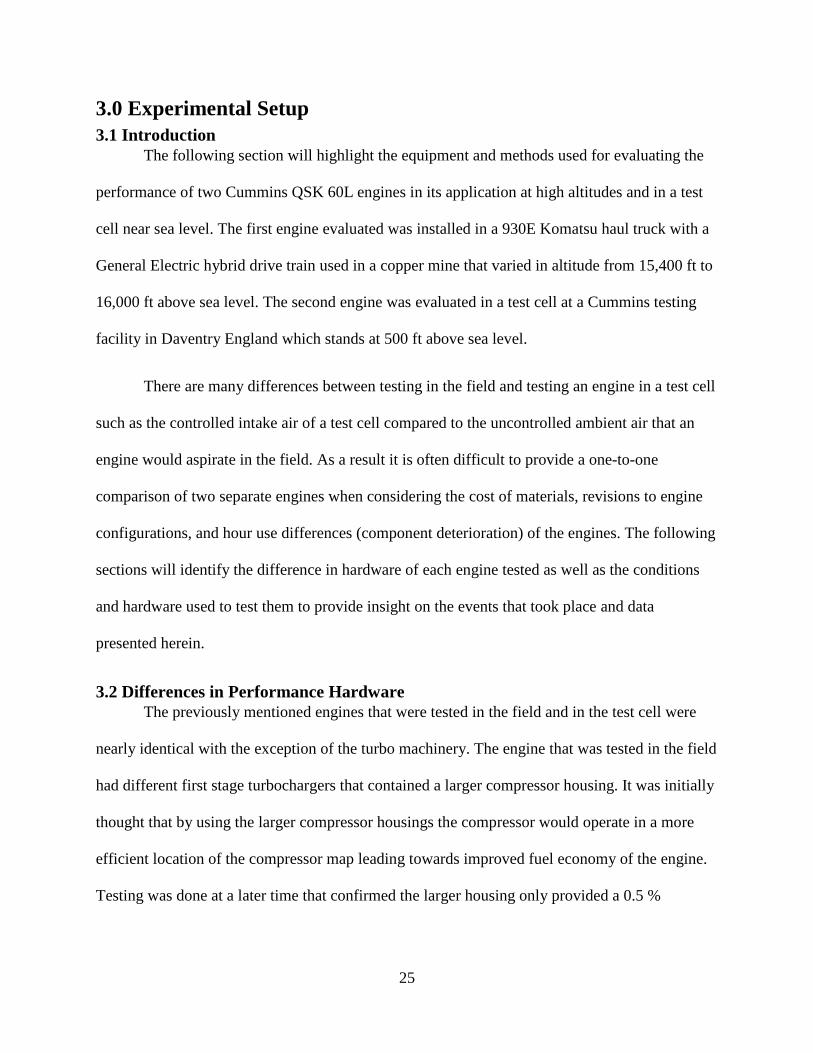
The following section will highlight the equipment and methods used for evaluating the

performance of two Cummins QSK 60L engines in its application at high altitudes and in a test

cell near sea level. The first engine evaluated was installed in a 930E Komatsu haul truck with a

General Electric hybrid drive train used in a copper mine that varied in altitude from 15,400 ft to

16,000 ft above sea level. The second engine was evaluated in a test cell at a Cummins testing

facility in Daventry England which stands at 500 ft above sea level.

There are many differences between testing in the field and testing an engine in a test cell

such as the controlled intake air of a test cell compared to the uncontrolled ambient air that an

engine would aspirate in the field. As a result it is often difficult to provide a one-to-one

comparison of two separate engines when considering the cost of materials, revisions to engine

configurations, and hour use differences (component deterioration) of the engines. The following

sections will identify the difference in hardware of each engine tested as well as the conditions

and hardware used to test them to provide insight on the events that took place and data

presented herein.

3.2 Differences in Performance Hardware

The previously mentioned engines that were tested in the field and in the test cell were

nearly identical with the exception of the turbo machinery. The engine that was tested in the field

had different first stage turbochargers that contained a larger compressor housing. It was initially

thought that by using the larger compressor housings the compressor would operate in a more

efficient location of the compressor map leading towards improved fuel economy of the engine.

Testing was done at a later time that confirmed the larger housing only provided a 0.5 %

26

improvement in turbo efficiency. This is considered a negligible difference when considering

measurement error. The compressor maps for both turbochargers tested can be seen in Figure 7.

Figure 6 Compressor maps for both turbochargers tested in the test cell [Cummins Holset: FAE Maps].

It can be seen that the turbocharger with the larger compressor housing, seen on the right,

has very similar map to the turbocharger with the smaller compressor housing, seen on the left in

Figure 6. With both compressors operating in the heart of their compressor maps with similar

efficiencies it can be seen that the there is little to no difference in operation with the exception

of rotor speed. As expected, the compressor with the larger housing was able to achieve the same

efficiency at a lower rotor speed; however, this did not contribute to improving to the

performance of the engine.

3.3 Field Data Collection

3.3.1 Test Cycle

The test cycle was defined by the normal operation of the mine haul truck for the

Caserones copper mine in the Andes Mountains. Haul trucks carrying copper mined in the Andes

run a unique duty cycle compared to trucks mining in other parts of the world. Most large mines

start mining at the surface and work their way down to create a “pit” mine. In this instance trucks

would drive down into the pit without a load, receive their load from the shovel, and drive fully

27

loaded out the pit to the location where they dump their load. Mining that occurs in the Andes

Mountain range starts from the top of the mountains and removes the material to a lower location

on the mountain. In this instance the trucks drive up the mountain with no load, receives the load

from the shovel, and drives down the mountain with the load to the dumping location. The

Caserones copper mine is located between 15,400 ft and 16,000 ft in elevation providing an

average barometric pressure of approximately 8.74 psia. Along with reduced barometric

pressures relative to sea level, temperature swings are also experienced at the mine. Most of the

field testing was conducted while temperatures were between 20 and 30° F, which provides

lower intake manifold temperatures than that seen near sea level during the laboratory testing.

Adding to the complexity of the duty cycle is the GE Hybrid drivetrain. This hybrid drive

train uses the power from the engine to generate electrical power to propel the truck but it can

also absorb power through large resistive banks, which is known as dynamic braking. The GE

system allows for six modes of operation on the truck. The first is idle, when the GE system is

disengaged and the truck is not moving. The second is “ready mode” when the throttle is

engaged to 25 % and low idle reaches 900 rpm. Ready mode is to maintain higher temperatures

and a state of operation that allows for faster transients. The third mode of operation is

everywhere on or below the torque curve of the engine and above the ready mode low idle. In the

fourth mode of operation, the truck is in a dynamic braking operating condition when the engine

is maintained at approximately 1600 rpm and the throttle is set to 65 %. This mode is unique to

the GE electric drive system in the way that it uses the engines speed to drive a fan on the

alternator to cool the alternator while it is absorbing power. Since the engine is only driving the

fan, and nothing more, this is considered a low load operating condition. The fourth mode of

operation is rated representing the maximum power the engine can create. This mode is typically

28

seen when the haul truck is climbing a hill or carrying its load. Finally, the last mode of

operation is when the truck is dumping its load and the GE system is engaged to power the

hydraulics of the truck. Figure 7 highlights a typical duty cycle for a haul truck in the Caserones

mine.

Figure 7 Duty cycle of a haul truck at the Caserones mine.

The first point of operation for a haul truck is backing up to the shovel, identified in

Figure 7 by segment 1. The truck then stays at idle while it gets loaded by the shovel (segment

2). The next point of operation identifies the pull away from the shovel and drive across a flat

towards the downhill route (segment 3). In the fourth operating segment, the truck remains in a

state of dynamic braking as it proceeds down the mountain. Then, in operating segment 5, the

truck reaches the downhill point and begins advancing to the dumping point. In segment 6, the

haul truck is in an idle state of operation while it waits in position to dump its load. Once the

bulldozer operator signals, the hydraulics for dumping the load are engaged, identified by

segment 7. After the load has been completely emptied and the bed of the truck is lowered the

vehicle immediately takes off and starts back up the mountain at rated conditions in segment 8.

In segment 9, the vehicle reached the top of the mountain and drives across the flat back towards

500

700

900

1100

1300

1500

1700

1900

120 340 560 780 1000 1220 1440 1660 1880

Engi

ne

Spee

d (

rpm

)

Time (sec)

1 2 3 4 5 6 7 8 9 10

29

the shovel. Lastly, the truck comes to a stop and makes several maneuvers to position itself next

to the bucket to be loaded again in segment 10.

To provide better insight on how the GE system loads the engine relative to the engines

torque curve, Figure 8 is provided below. It can be seen that the engine can provide a great deal

more power below 1700 rpm but the GE electric drive system does not utilize this potential.

Figure 8 Torque curve from test cell compared to the GE loading curve in a haul truck.

Cummins has instrumented vehicles with data loggers and have determined that

approximately 25 % of a haul truck’s duty cycle is spent at rated conditions, while 15 % is spent

in ready mode, but these numbers do vary from based on the mine site’s geography. This can be

seen below in Table 2.

0

1000

2000

3000

4000

5000

6000

7000

8000

500 700 900 1100 1300 1500 1700 1900 2100

Engi

ne

Torq

ue

(ft-

lb)

Engine Speed (rpm)

GE Load Curve Test Cell Torque Curve

Ready ModeDyn. Braking

Dumping Rated

30

Table 2 shows the time spent at each operating mode for a haul truck in a pit mine.

The data provided in Table 2 came from a haul truck that was operating in a pit mine

where the vehicle would be in a dynamic braking state of operation with no load into the pit and

would then be a rated conditions for a greater amount of time coming out of the mine. This is just

one example of the duty cycle of a haul truck.

3.3.2 In-Cylinder HSDA System

An AVL INDIMICRO™ was utilized as the HSDA system to capture the injection

signal, the in-cylinder pressure signal, the intake manifold pressure, the speed of the engine, and

the trigger used for crankshaft location [INDIMICRO™]. The INDIMICRO™ features four

analog or four digital signal inputs that can be utilized at the discretion of the user along with a

speed and trigger inputs.

31

Figure 9 AVL INDIMICRO™ unit with an AVL Vehicle Interface module used during field testing.

To capture the dynamic in-cylinder pressure, an AVL GU21-D piezoelectric pressure

transducer was used in conjunction with a 50 ft low noise cable. The injection signal was

captured via an in-house fabricated Wheatstone bridge style strain gage mounted to the rocker

lever that engages the push rod for the injection to occur. The trigger and speed signal utilized a

magnetic pickup sensor to provide an analog signal to the INDIMICRO™. Lastly, the intake

manifold pressure sensor utilized the diaphragm styled OEM sensor already instrumented on the

engine to receive an analog input to the INDIMICRO™.

All of the signals were monitored in real time using the complimentary software that is

used to set up and operate the INDIMICRO™. The post processing, however, was done by an

additional AVL software called AVL Concerto. Concerto is a user-based software that has basic

filtering and mathematics macros within the software that allow the user to build more complex

macros to perform the analysis they desire. Cummins has defined standardized methods of post

processing pressure data which are built into macros that were made available for this effort.

32

3.3.3 Cylinder Pressure

The dynamic in-cylinder pressure was recorded using a piezoelectric pressure transducer

manufactured by AVL. Internal to the pressure transducer is a quartz crystal and when exposed

to a pressure change emits a charge relative to that pressure change. This charge is transmitted

through low noise cables to a charge amplifier that is internal to the INDIMICRO™. The

software that comes with the INDIMICRO™ allows inputs from the manufacturer of the

pressure transducer stating the sensitivity of the pressure transducer when it was calibrated.

These values are usually on the order of 200 psi/pico-Coulomb. From the charge amplifier, the

signal is read into the HSDA system at a rate relative to the engine speed.

3.3.4 Trigger and Speed

The trigger signal was used along with a reference cylinders motoring curve to define the

position of the crankshaft. The motoring curve provided a top dead center of the reference

cylinder using the assumption that the peak in-cylinder pressure occurred at top dead center

when motoring the engine. To produce the motoring curve, an injector hold down tool was used

to seat the injector needle on the nozzle preventing any fuel from being injected.

A custom tone wheel with one rectangular tooth was mounted to the fan hub that attaches

to the damper at the front of the engine for the purpose of provide an indicated trigger for the

relative position of the crank to the reference cylinder. A robust mount was fabricated such that a

magnetic pickup sensor was positioned directly over the tooth of the tone wheel. With each

revolution the magnetic pickup sensor produced a voltage signal that had a frequency and

magnitude relative to the speed. This signal was received by a Hoffer signal conditioner that

turned the low voltage signal into a five volt TTL signal with the same frequency. This signal

was sent directly to the INDIMICRO™ where it was saved simultaneously with the rest of the

data.

33

The speed of the engine was acquired using the Cummins magnetic pick up sensor

mounted in the flywheel housing of the engine. The speed signal, along with the trigger signal,

allowed for the data to be post processed on a crank angle basis.

3.3.5 Injection

The injection signal was retrieved by mounting a Wheatstone bridge styled strain gage to

the top of the rocker lever that engaged the plunger on the injector. When the cam would begin

lifting the rocker lever the strain in the rocker lever was sensed by creating by changing the

resistance in the Wheatstone bridge equivalent to the strain within the material. The voltage

difference caused by this resistance change was translated back to a charge amplifier which was

then relayed as an analog in signal to the INDIMICRO™. Note that because of post processing

requirements, this data was not available for this analysis.

3.3.6 IMP

The IMP (intake manifold pressure) or boost pressure was recorded by utilizing the

factory IMP sensor used with the ECM software. The diaphragm style pressure sensor sent its

signal to the INDIMICRO™ via an analog signal on low noise cables. The factory values

associated with the amount of pressure per voltage were entered into the INDIMICRO™ such

that is could convert the voltage into the appropriate pressure units.

This signal was used during the pegging process of the pressure curve. At the start of the

compression stroke, after the valve closed, the in-cylinder pressure was assumed to be equal to

the IMP. Since the piezoelectric transducers only created a charge relative to a pressure and are

susceptible to hysteresis there must be some known value to make the signal relative, which was

set to be the IMP. When the signals were processed, the starting in-cylinder pressure was set

equal to the boost pressure measured by the IMP sensor and the pressure measured by the in-

cylinder pressure transducer was added onto this pressure.

34

3.3.7 IMEP

IMEP (indicated mean effective pressure) is a metric used to evaluate the amount of work

that was created by an engine relative to the displacement of the engine. Using the

thermodynamic relationship for piston work, the integral can be taken of the pressure curve

relative to the cylinder volume to determine the indicated work. Integrating between -180° CA

and +180° CA encompasses the compression and expansion strokes, thus providing the sum of

the work lost to compressing the charge and the work gained from the combustion. The same

calculation can be done over the duration of the intake and exhaust strokes to evaluate the

negative work the engine does to pull the air into the combustion chamber as well as push the

exhaust gasses out of the chamber, referred to as the low pressure pumping losses. The indicated

work in both cases is divided by the displacement of the engine to provide the IMEP and PMEP

(pumping mean effective pressure). This calculation was done during post processing via a

Cummins macro in Concerto.

3.3.8 HRR

The apparent HRR was calculated using the post processing tool Concerto provided by

AVL. Within Concerto, macros were assembled in which the inputs for HRR were the pegged

dynamic pressure, crank angle of intake valve closing, and the intake manifold temperature.

The macro calculated a specific heat ratio as a linear function of the bulk gas temperature

in Rankine. The bulk gas temperature was calculated using the ideal gas equation with an added

reheat of 520 R. The additional 520 R was used to account for the temperature increase of the

fresh charge from the mixing with residual gases and heat transfer from the cylinder walls.

𝛾 = 1.4 − (7.185 × 10−5 × 𝐵𝑢𝑙𝑘 𝐺𝑎𝑠 𝑇𝑒𝑚𝑝)

35

This specific heat value, the pegged dynamic in-cylinder pressure, and the calculated

cylinder geometry made up the basis of the HRR calculation. Once the curve was defined, a

robust double Gaussian filter was applied to filter the early portion of combustion to preserve the

characteristics of the premix combustion while the diffusion combustion was filtered less heavily

since it was generally smoother by nature.

3.3.9 Thermal Efficiency

The gross thermal efficiency was defined for this effort as the indicated work derived

from the dynamic pressure signal divided by the mass of fuel injected multiplied by the heating

value of the fuel [Heywood, 1988].

𝜂𝑓 =𝑊𝑐

𝑚𝑓 × 𝑄𝐻𝑉

The heating value of the fuel was a value provided by an analysis consistent with ASTM D-

3338. The mass of the fuel injected was calculated from the amount of metered fuel injected that

was estimated by the engine calibration and the specific gravity provided by ASTM D-4052.

3.3.10 Heat Release

Heat release was calculated by integrating the HRR curve from -60° CA to 180° CA. By

doing this the valve events are missed and are not accounted for when considering the amount of

fuel energy is converted to mechanical work. From the heat release, the total amount of fuel that

was converted to work can be quantified and normalizing the heat release curve can provide

further insight on what rate and crank angle location the fuel was burning at.

3.3.11 Mass Fraction Burned

The MFB was defined as the percent of fuel burned at a given crank location relative to

the total apparent HR calculated. Utilizing the normalized heat release curve, the mass of fuel

36

burned is assumed to be proportional to the amount of heat release from the normalized 0 % to

100% heat release curve. The MFB was calculated using a Cummins macro in Concerto.

3.3.12 Ignition Delay

The ignition delay was calculated by using the difference in what was commanded in the

calibration for injection timing and the start of combustion. The start of combustion was defined

as the moment the HRR curve becomes 0 BTU/CA between -20° CA and top dead center.

3.3.13 Maximum In-Cylinder Pressure

The maximum in-cylinder pressure was determined by averaging 100 consecutive

pressure curves during steady state operation using a Cummins developed macro in AVL

Concerto. The maximum value from the 100-average pressure traces was specified as the

maximum in-cylinder pressure.

3.4 Test Cell Data Collection

3.4.1 Test Cell Hardware/ Instrumentation

As previously mentioned, the test cell portion of testing was conducted at Cummins

testing facility in Daventry, England. The engine was mounted to a test skid and connected to a

Froude F47 water brake dynamometer. While under test, the dynamometer controlled speed by

water flow rate, thus changing the resistance in the dynamometer, while the test cell controlled

the commanded throttle which set the load. The torque was measured by a strain gage sensor

mounted to the side of the dynamometer and was reported to the operator’s computer.

The test cell was equipped with an overhead junction box that acted as a central location

where all of the instrumentation would connect prior to going to the test cell. Included in this

overhead junction box was a 9-pin connector that provided all of the engine controller’s signals

to the laboratory data acquisition system. E-type thermocouples were used for the temperature

readings for all of the working fluids of the engine and test cell including, oil, coolant, fuel,

37

intake air, and exhaust. Various diaphragm-styled pressure transducers were used for the

pressure measurements for the test cell and the engine. The pressures measured include exhaust

port pressures, pressures across the turbocharger on both the intake and exhaust side, IMP, fuel

pressure, coolant pressure, and oil pressure. The fuel mass flow rate was measured by a Coriolis

meter and the intake air flow rate was measured with a venturi styled meter while the exhaust

flow rate was calculated based on the sum of the fueling and intake air measurements.

Shell and tube heat exchangers were used for the controlling the temperatures of the after

cooler cooling circuit and the engine block cooling circuit. The shell and tube used were an air-

to-liquid (intercooler) and a liquid-to-liquid (engine block coolant) style heat exchangers where

the process water flow rate was controlled via a valve position actuator. The same liquid-to-

liquid style heat exchanger was used, but on a smaller scale, to control the temperature of the

fuel. Cummins facilities maintained an air handling system that controlled the temperature and

dew point of the intake air within 1° C for all the test cells using an advanced HVAC system.

The intake and exhaust restrictions were set by actuated valves at the operator’s console. The

blow-by of the engine was monitored using an OEM orifice style volumetric flow meter and was

primarily used for test cell safety limits.

3.4.2 In-Cylinder HSDA System

The HSDA system used consisted of six major components: installation hardware,

transducer, cabling, charge amplifier, data acquisition card, and software. At the engine, the

cylinder heads were drilled and tapped to accept the in-cylinder pressure transducers. The

cylinder heads were drilled at an angle such that that a sleeve was inserted through a freeze plug

hole into the coolant passage and finally through the head in the cylinder. The pressure

transducer was then inserted within the sleeve such that the face of the transducer was exposed to

38

the combustion chamber. The transducers used in the test cell were AVL QC34C pressure

transducers. This model of transducer was water cooled making it less susceptible to thermal

shock. Attached to the pressure transducers were low noise cables that relayed the charge signal

to the AVL 4P3G charge amplifiers. It is here where the amplifiers were set up with the pressure

transducers sensitivities and amplified the signal. The amplified signal was converted into an

analog signal and sent to an AVL analog-to-digital converter card within the test cell computer.

The signal was then interpreted using AVL Indicom v2.6 software.

The pressure recorded with the in-cylinder transducer, and associated amplifier, is only a

relative value. This pressure signal was adjusted to actual pressure at the start of the

measurement using the intake manifold pressure. However, the Indicom software incorporated a

‘Thermodynamic Zero Level Correction’ process for steady state operation. Their pegging

process assumes an adiabatic compression process in which they can employee a constant

polytropic coefficient and the engine geometry to determine what the pressure was between -

100° CA and -65° CA [AVL User’s Guide, 2013]. The pressure signal recorded with the AVL

system is then processed to the calculated pressure.

Working in conjunction with the HSDA system was a 1440 count per revolution BEI

optical encoder that was mounted to the front of the engine via a shaft coupling damper. The

optical encoder provided the engine speed and position to interpret the pressure on a crank angle

basis with a 0.25° CA resolution.

With all of the above listed instrumentation and knowledge of the engines geometry and

firing order, every cylinder that was instrumented can be evaluated to determine efficiencies and

mechanical occurrences on a crank angle basis.

39

3.4.3 Test Condition

Test conditions were maintained the same within the test cells ability for all operating

conditions with the exception of the intake and exhaust restrictions. The engine had two coolant

loops to control; one going through the after coolers and the other moving through the jacketing

of the engine heads and block. The after cooler loop was commanded to maintain a temperature

of 57° F with a tolerance of ± 1° F. The water jacketing coolant temperature was commanded to

be 82° C with a tolerance of ± 1° F. The intake air was controlled to 25° C while the dew point

was set to 15° C. Fuel temperatures were maintained at 40° C with a tolerance of ±1° C.

The intake and exhaust restrictions were set to 15 inH2O and 20.35 inH2O, respectively,

at rated operating conditions; 2500 hp at 1900 rpm. Once the restrictions were set, they were

locked in open loop and not controlled with the operation of the engine. The barometric pressure

of the intake air was not controlled and was thus equal to the atmospheric pressure at the

facilities elevation at 500 ft above sea level and varied with local atmospheric weather

conditions.

3.4.4 Test Cycle

Normal test operation consisted of multiple daily checks to ensure no wires or hose were

out of place and that all fittings were properly tightened. The engine fluids levels were checked

prior to starting the engine. After starting the engine, a second walk through was done while the

engine was at idle to check for leaks. Once the engine was determined to be operating normally,

the test cell operator slowly increased the speed and load until the rated operating condition of

1900 rpm and 2500 hp were met. The engine was provided five minutes to stabilize before

recording data for 60 seconds. The recorded data was averaged and then reviewed to ensure all

measurements were being collected properly and that there were no deficiencies such as boost or

fuel leaks. The engine was brought to idle while a test script was prepared. Data at this rated

40

condition was taken consecutively every six hours of testing or if there was a suspicion of the

engine not operating properly.

All testing conducted in the test cell was at a steady state conditions. The engine was

brought from idle to the first operating point with the minimal amount of load on the engine and

allowed to stabilize for five minutes. Once the engine stabilized data was recorded, again taking

the average over a 60 second period. Once the data point was taken and verified to be recorded

properly the engine was then moved to the next operating point. For efficiency, test scripts were

created that would control the engine operation autonomously.

It is noted that the test operating conditions and the in-field operating conditions are

different. There are many factors that come into play when considering a large complex system

of a haul truck that incorporates the interaction of a driver, the engine, and the GE electric

system. It is for this reason that there will be several differences of the commanded operating

parameters of the vehicle between the test cell engine and the engine tested in its application.

41

4.0 Results and Discussion

4.1 Introduction

The following sections will discuss in detail the data that was recorded from a Cummins

QSK 60L, V16 diesel engine with a two stage turbocharging air handling system in the test cell

as well as in a haul truck in the field. There were four modes of steady state operation witnessed

in the haul truck and included ready mode, dynamic braking, rated, and dumping. Because of

limited in-field data for the ready mode, only the data from the three remaining modes will be

discussed in detail. Select engine control parameters for three modes are summarized in Table 3

and were used for the primary evaluation in this effort. Pressure data from both tests were

collected and reduced to compare the operation of each engine with one operating in the field at

15,800 ft and the other in an engine dynamometer test cell near sea level.

Table 3 shows the steady state operating conditions chosen to evaluate for this effort.

Dynamic Braking Rated Dumping

Test Location

Field

Test

Test

Cell

Field

Test

Test

Cell

Field

Test

Test

Cell

Engine Speed (RPM) 1570 1600 1900 1900 1900 1900

Commanded Fueling (mm3/Inj.) 85 94 531 546 140 151

Commanded Inj. Timing (°BTDC) 9.8 10 6.6 7 10 10.5

4.2 Test Cell Data Reduction

The focus of this section will be the pressure data gathered from cylinders 1 left and 8

right in a test cell setting. It is valuable to start with evaluating the pressure curves of two

different cylinders to quantify the cylinder-to-cylinder variation an engine may have.

4.2.1 Rated Operation Pressure Analysis

The pressure curve for rated operating conditions can be seen in Figure 10.

42

Figure 10 Pressure curves for cylinders 1 left and 8 right at rated conditions.

It can be seen that there is little variation between the two cylinders for rated operating

conditions with each cylinder reaching a peak pressure of approximately 2640 psi. Two different

‘runs’ were conducted at the same operating point and were compared to identify the stability of

the operating point. It was identified that the difference in the maximum pressure between each

cylinder was approximately 0.19 % for run 1 and 0.78 % on run 2. Also, it was shown that the

difference in maximum in-cylinder pressure between each run was 0.6 % for cylinder 8 right

where there was no difference for cylinder 1 left. Based on these results, it can be said that there

is little variation in the peak in-cylinder pressure from cylinder-to-cylinder as well as between

the two different runs showing high stability in this operating point. Another useful metric

derived from the in-cylinder pressure curve was the IMEP. After deducing the positive work

done relative to the displacement of the cylinder the IMEP was found to be 338 psi for cylinder 8

right with a negligible difference between runs and 340 psi for cylinder 1 left with a 1.19 %

difference between each run. The IMEP values as well as the previously discussed maximum in-

cylinder pressure are displayed in Table 4.

0

500

1000

1500

2000

2500

3000

-180 -150 -120 -90 -60 -30 0 30 60 90 120 150 180

Pre

ssu

re (

psi

)

Crank Angle

1 Left Run 1 8 Right Run 1 1 Left Run 2 8 Right Run2

43

Table 4 Provides pertinent information derived from the pressure curve for the rated mode of operation.

Cyl 1L

PCP

Cyl 8R

PCP

Cyl 1L

PCP

Cyl 8R

PCP

Cyl 1L

IMEP

Cyl 8R

IMEP

Cyl 1L

PMEP

Cyl 8R

PMEP

psi psi CA CA psi psi psi psi

Run 1 2648.2 2643.1 8 8 340.48 338.27 -8.34 -6.48

Run 2 2648.1 2627.5 8.4 8.3 336.46 338.94 -8.71 -7.21

It can be seen in Table 4 by evaluating the PMEP that cylinder 1 left required more work

than cylinder 8 right to pull the fresh air charge into the cylinder as well as expel the exhaust

gasses. This may indicate that less air was received by cylinder 1 left and provide a reason for

lower maximum in-cylinder pressures.

Taking the pressure analysis a step further, the HRR was calculated to evaluate the

energy conversion of the fuel to mechanical work as shown in Figure 11. As illustrated in this

figure, the derived HRR from the two cylinders showed good comparison and good repeatability

with a maximum percent difference of 0.43 % between runs 1 and 2, and 0.25 % between each

cylinder.

Figure 11 HRR curve for cylinders 1 left and 8 right at rated operating conditions.

Figure 11 shows that there was visibly no separation between the premix burn fraction

and the diffusion burn fraction. Also provided by the heat release analysis was the presumed start

of combustion and consequently the ignition delay. The start of combustion was unable to be

-0.1

0

0.1

0.2

0.3

0.4

0.5

0.6

0.7

-30 -25 -20 -15 -10 -5 0 5 10 15 20 25 30 35 40 45 50 55 60

Hea

t R

elea

se R

ate

(BTU

/CA

)

Crank Angle

1 Left Run 1 8 Right Run 1 1 Left Run 2 8 Right Run 2

44

determined due to the fact the HRR became negative prior to the commanded injection timing.

The differences in maximum HRR and the location they occurred at can be observed in Table 5.

Table 5 Maximum HRR and location it occurred.

Cyl 1L Ign.

Delay

Cyl 8R Ign.

Delay

Cyl 1L Max

HRR

Cyl 8R Max

HRR

Cyl 1L Max

HRR

Cyl 8R Max

HRR

∆CA ∆CA BTU/CA BTU/CA CA CA

Run 1 3 4.5 0.176 0.140 -1 0

Run 2 3.5 4 0.178 0.162 -1 -0.5

By integrating the HRR curve the heat release curve is reduced. It can be seen in Figure

11 that by evaluating the heat release curve the MFB, the total energy converted to work from

the injected fuel, and the thermal efficiency can all be derived. Consistent with the other in-

cylinder pressure analysis information, the heat release curve shows repeatability between the

two runs as well as between the different cylinders. The maximum heat release exhibited was

16.68 BTU from cylinder 1 left with the maximum difference between cylinders was 1.87 %

while the maximum differences between both runs was 2.49 %. Most notable, was the

repeatability exhibited by cylinder 8 right with a 0.0 % difference between runs 1 and 2 at 16.57

BTU.

Figure 12 Heat release curve for rated operating conditions for cylinder 1 left and 8 right.

-0.2

1.8

3.8

5.8

7.8

9.8

11.8

13.8

15.8

17.8

-30 -20 -10 0 10 20 30 40 50 60 70 80 90 100 110 120

Hea

t R

elea

se (

BTU

)

Crank Angle

1 Left Run 1 8 Right Run 1 1 Left Run 2 8 Right Run 2

45

The MFB, describing the mass of fuel converted to heat, was identified by normalizing

the curve seen in Figure 12 and identifying the location where 10 %, 50 %, and 95 % of the fuel

was burned relative to the maximum heat release. This is useful to conceptualize the rate at

which the fuel is burned throughout the expansion stroke. The results of the MFB can be seen in

Table 6. Interesting to note from Table 6 is the repeatability of cylinder 8 right between runs 1

and 2, all of which remained below 0.2° CA difference. Cylinder 1 left, however, proved to be

less repeatable with a maximum difference of location between cycles of 6.56° CA for the 95 %

MFB and a minimum of 0.65° CA for the 10 % MFB location.

Table 6 MFB results for rated operating conditions.

10% MFB (CA) 50% MFB (CA) 90% MFB (CA) 95% MFB (CA)

Cyl 1L Cyl 8R Cyl 1L Cyl 8R Cyl 1L Cyl 8R Cyl 1L Cyl 8R

Run 1 4.10 3.77 17.97 17.53 40.18 42.22 54.71 63.87

Run 2 3.45 3.80 17.12 17.48 36.93 42.66 48.14 64.03

Difference 0.65 0.03 0.85 0.04 3.25 0.44 6.56 0.16

Using the maximum heat release, indicated thermal efficiency was calculated. The

maximum indicated thermal efficiency was found to be 44.76 % from cylinder 8 right on run 2.

Continuing with the same trend as the rest of the rated data is the minimal difference among the

cylinders as well as between runs. The maximum difference between cylinders was 0.95 % while

the minimum was found to be 0.44 %.

4.2.2 Dumping Operation Pressure Analysis

The next steady state mode of operation to discuss is dumping. This is representative of

when a haul truck is dumping its load, primarily utilizing the hydraulic system on the vehicle.

Compared to the rated mode of operation, dumping is considered to be a low load point of

operation and thus requires a small rate of fueling and consequently reduced in-cylinder pressure.

The in-cylinder pressure curve for the dumping mode of operation can be seen in Figure 13.

46

Figure 13 Pressure curve for a simulated dumping mode of operation.

As illustrated in Figure 13, there are obvious differences in the maximum pressures

between cylinders. The maximum pressure seen in cylinder 1 left was approximately 1178 psi

with a negligible difference between the each run. In cylinder 8 right, the maximum peak

pressure witnessed was 1215 psi with a 0.59 % difference between runs. Between the two

cylinders there was a maximum percent difference of 3.2 %. The maximum cylinder pressures

along with pressure derived information can be seen in Tables 7. It should be noted that for the

sake of maintaining reasonably short names in the tables the notation of PCP (peak cylinder

pressure) was implemented for the maximum in-cylinder pressure for each cylinder.

Table 7 Maximum cylinder pressure and pertinent information derived from the pressure curve for the dumping mode of

operation.

Cyl 1L

PCP

Cyl 8R

PCP

Cyl 1L

PCP

Cyl 8R

PCP

Cyl 1L

IMEP

Cyl 8R

IMEP

Cyl 1L

PMEP

Cyl 8R

PMEP

psi psi CA CA psi psi psi psi

Run 1 1178.1 1215.7 7.3 8.5 90.23 98.51 -7.42 -6.65

Run 2 1177.6 1208.6 7.2 8.4 92.12 98.25 -7.59 -6.89

The IMEP was derived from the pressure curve and was found to be 90.23psi and 92.12

psi for runs 1 and 2 on cylinder 1 left, respectively. The IMEPs for cylinder 8 right were 98.51

psi and 98.25 psi for runs 1 and 2, respectively, providing the least difference of 0.26 % while

0

200

400

600

800

1000

1200

1400

-180 -150 -120 -90 -60 -30 0 30 60 90 120 150 180

Pre

ssu

re (

psi

)

Crank Angle

1 Left Run 1 8 Right Run 1 1 Left Run 2 8 Right Run 2

47

cylinder 1 left showed differences as high as 2.05 %. The difference between the cylinders,

regarding IMEP were found to be 9.17 % for run 1 and 6.65 % for run 2. Again, cylinder 1 left

provided lower peak cylinder pressures for both runs as well as exhibited lower PMEP values

indicating that more work was required during the low pressure pumping events. Also worth

noting is the ringing in the pressure data where combustion is expected to be occurring. This

increased variation is attributed to in-cylinder pressure fluctuations from combustion.

The next step in the continuation of reducing the pressure curve is looking at the HRR

curve for the simulated dumping mode of operation found in Figure 14.

Figure 14 HRR curve for dumping mode of operation.

The premix burn fraction is more apparent in Figure 14 as compared to the rated

operating condition which was presumed to be from lower combustion stability. As previously

mentioned, there was a notable difference between the two cylinders while still maintaining

repeatability between the two different runs. Cylinder 1 left was shown to have a maximum HRR

of 0.200 BTU/CA for run 1 and 0.203 BTU/CA for run 2 where cylinder 8 right had maximum

HRR of .220 BTU/CA for both runs. This suggested that there were a negligible differences in

the maximum HRR for cylinder 8 right between each run and a 1.39 % difference between each

-0.01

0.04

0.09

0.14

0.19

0.24

-30 -25 -20 -15 -10 -5 0 5 10 15 20 25 30 35 40 45 50 55 60

Hea

t R

elea

se R

ate

(BTU

/CA

)

Crank Angle

1 Left Run 1 8 Right Run 1 1 Left Run 2 8 Right Run 2

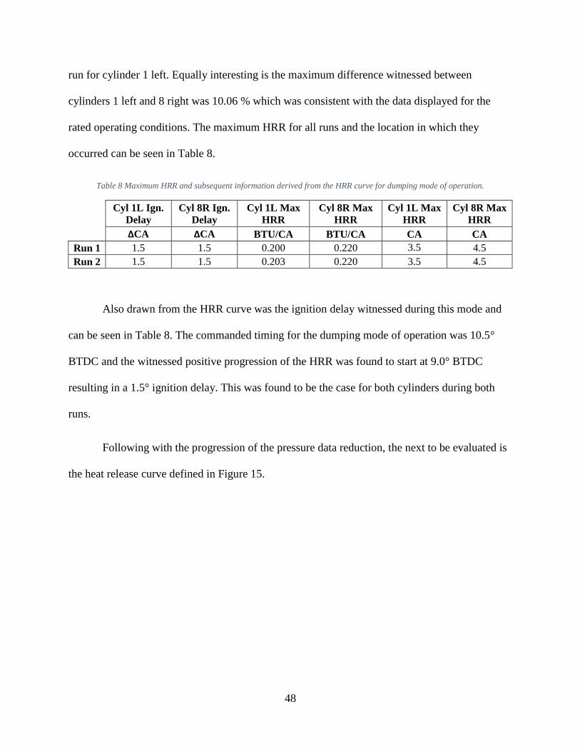
48

run for cylinder 1 left. Equally interesting is the maximum difference witnessed between

cylinders 1 left and 8 right was 10.06 % which was consistent with the data displayed for the

rated operating conditions. The maximum HRR for all runs and the location in which they

occurred can be seen in Table 8.

Table 8 Maximum HRR and subsequent information derived from the HRR curve for dumping mode of operation.

Cyl 1L Ign.

Delay

Cyl 8R Ign.

Delay

Cyl 1L Max

HRR

Cyl 8R Max

HRR

Cyl 1L Max

HRR

Cyl 8R Max

HRR

∆CA ∆CA BTU/CA BTU/CA CA CA

Run 1 1.5 1.5 0.200 0.220 3.5 4.5

Run 2 1.5 1.5 0.203 0.220 3.5 4.5

Also drawn from the HRR curve was the ignition delay witnessed during this mode and

can be seen in Table 8. The commanded timing for the dumping mode of operation was 10.5°

BTDC and the witnessed positive progression of the HRR was found to start at 9.0° BTDC

resulting in a 1.5° ignition delay. This was found to be the case for both cylinders during both

runs.

Following with the progression of the pressure data reduction, the next to be evaluated is

the heat release curve defined in Figure 15.

49

Figure 15 Heat release curve for dumping mode of operation.

The maximum heat release recorded was witnessed in cylinder 8 right at 4.75 BTU with a

0.19 % difference between run 1 and run 2. It was expected that cylinder 8 right would release

more heat since it had a larger HRR in the diffusion combustion burn fraction than cylinder 1 left

which showed to have a maximum heat release of 4.35 BTU during the second run. It was found

that cylinder 1 left was shown to have a maximum difference of 2.41 % between each run

showing there was less stability witnessed in that cylinder as compared to cylinder 8 right.

Next in the evaluation of the heat release curve is the MFB. The results for the dumping

mode of operation are defined in Table 9.

Table 9 Location of MFB for the dumping mode of operation.

10% MFB (CA) 50% MFB (CA) 90% MFB (CA) 95% MFB (CA)

Cyl 1L Cyl 8R Cyl 1L Cyl 8R Cyl 1L Cyl 8R Cyl 1L Cyl 8R

Run 1 -3.02 -3.11 6.40 6.75 23.80 30.55 30.99 56.86

Run 2 -2.96 -3.07 6.51 6.87 24.46 31.16 32.19 59.00

Difference 0.06 0.04 0.10 0.12 0.65 0.61 1.20 2.15

Further backing the assessment of ignition delay is the small differences in the location in

which 10 % MFB occurs for both cylinders and both runs. This is also the case between runs for

the 5 0% MFB with a maximum degree crank angle difference of 0.12° CA exhibited from

cylinder 8 right. The most noteworthy result is from the 95 % MFB assessment. While the largest

-0.2

0.8

1.8

2.8

3.8

4.8

5.8

-30 -20 -10 0 10 20 30 40 50 60 70 80 90 100 110 120

Hea

t R

elea

se (

BTU

)

Crank Angle

1 Left Run 1 8 Right Run 1 1 Left Run 2 8 Right Run 2

50

degree crank angle difference was witnessed from cylinder 8 right between run 1 and 2 at 2.15°

CA the difference between cylinders 1 left and 8 right is over 20° CA. These results imply that

cylinder 8 right sustained combustion for a longer duration of time while combustion in cylinder

1 left ended around 31° CA.

Concluding the pressure analysis for the dumping mode of operation is the thermal

efficiency assessment that was derived from the maximum heat release. Cylinder 8 right

provided a higher indicated thermal efficiency than cylinder 1 left with a maximum value of

46.76 %. The maximum value witnessed from cylinder 1 left was 43.73 % with a difference of

2.09 % between runs 1 and 2 where cylinder 8 right only had a difference of 0.26 % between

each run.

4.2.3 Dynamic Braking Operation Pressure Analysis

The final operating mode being evaluated in this effort is dynamic braking. Dynamic

braking was characterized as a low load operating point relative to the rated operating point and

on the same order as the dumping mode of operation but at a lower operating speed. The

dynamic in-cylinder pressure curve for dynamic braking is displayed in Figure 16.

Figure 16 shows the pressure curves for the dynamic braking operating mode.

0

100

200

300

400

500

600

700

800

900

1000

-180 -150 -120 -90 -60 -30 0 30 60 90 120 150 180

Pre

ssu

re (

psi

)

Crank Angle

1 Left Run 1 8 Right Run 1 1 Left Run 2 8 Right Run 2

51

It is visually apparent in Figure 16 that there was a larger difference in pressure amongst

all of the cylinders as well as between runs relative to the previous two modes of operation

evaluated. The highest maximum in-cylinder pressure witnessed was in cylinder 1 left at 897.6

psi on run 1. Run 2 on cylinder 1 left provided a maximum in-cylinder pressure of 863.1 psi

which was a 4 % difference from run 1. Cylinder 8 right showed a similar difference of 3.77 %

between runs 1 and 2 with the maximum pressure of 848.8 psi on run 2. These values along with

the mean effective pressure assessment can be seen in Table 10.

Table 10 Maximum in-cylinder pressures and pertinent information derived from the pressure curve for dynamic braking mode of

operation.

Cyl 1L

PCP

Cyl 8R

PCP

Cyl 1L

PCP

Cyl 8R

PCP

Cyl 1L

IMEP

Cyl 8R

IMEP

Cyl 1L

PMEP

Cyl 8R

PMEP

psi psi CA CA psi psi psi psi

Run 1 888.58 831.83 5 5 44.85 32.07 -6.02 -4.84

Run 2 863.05 848.77 5.5 4.9 41.74 39.62 -6.00 -5.56

The dynamic braking mode has been the first mode of operation where cylinder 1 left

provided consistently higher values than cylinder 8 right. This is again made evident in the IMEP

assessment where cylinder 1 left had higher IMEP values and a lower difference between runs

compared to cylinder 8 right. Cylinder 1 left showed IMEP values of 46.93 psi for run 1 and

41.73 psi for run 2 providing a difference of 12.42 % whereas cylinder 8 right had 29.87 %

difference between runs with 27.78 psi for run 1 and 39.62 psi for run 2. Also of importance was

the PMEP exhibited by cylinder 1 left. It can be seen in Table 10 that just like the other modes of

operation cylinder 1 left provided a greater negative work compared to cylinder 8 right. Despite

this it still managed to provide higher peak cylinder pressures.

It was expected that the trend of cylinder 8 right continued to have lower values occur

and was observable in the HRR curve in Figure 17.

52

Figure 17 shows the HRR curve for the dynamic braking mode of operation.

Illustrated in Figure 17, it can be seen that there was a very prominent premix combustion

event happening over a short period of crank angle followed by a sustained diffusion

combustion. It is noted that premix combustion is often the more uncontrolled combustion phase

and contributes to more variability within combustion. As expected, cylinder 8 right had a lower

maximum HRR of 0.138 BTU/CA and 0.162 BTU/CA for runs 1 and 2 resulting in 14.59 %

difference between the two runs. Cylinder 1 left showed a maximum HRR 0.181 BTU/CA for

run 1 and 0.178 BTU/CA for run 2 and resulted in a 1.47 % difference between the runs. With

these results it should be noted that there was a 23.37 % difference in maximum heat release

between cylinders 1 left and 8 right on run 1 and an 8.96 % difference during run 2. This was the

largest difference observed from all modes of operation. The maximum HRR values along with

subsequent values derived from the HRR curve can be seen in Table 11.

Table 11 Maximum HRR, the location of maximum HRR, and ignition delay for dynamic braking mode of operation.

Cyl 1L Ign.

Delay

Cyl 8R Ign.

Delay

Cyl 1L Max

HRR

Cyl 8R Max

HRR

Cyl 1L Max

HRR

Cyl 8R Max

HRR

∆CA ∆CA BTU/CA BTU/CA CA CA

Run 1 3 4.5 0.176 0.140 -1 0

Run 2 3.5 4 0.178 0.162 -1 -0.5

-0.01

0.04

0.09

0.14

0.19

-30 -25 -20 -15 -10 -5 0 5 10 15 20 25 30 35 40 45 50 55 60

Hea

t R

elea

se R

ate

(BTU

/CA

)

Crank Angle

1 Left Run 1 8 Right Run 1 1 Left Run 2 8 Right Run 2

53

The difference in degrees crank angle between runs 1 and 2 was 0.5° CA for both

cylinders. The ignition delay observed in cylinder 1 left was 3.0° CA for run 1 and 3.5° CA for

run 2. Consistent with the large variation seen in this mode of operation was the fact that cylinder

1 left advanced by a 0.5° CA from run 1 to run 2 while cylinder 8 right did the opposite.

Cylinder 8 right provided an ignition delay of 4.5° CA in run 1 and 4.0° CA in run 2.

Looking next to the heat released, it was expected to see large variation between

cylinders in the maximum heat release, which is displayed below in Figure 18.

Figure 18 shows the heat release curve for the dynamic braking mode of operation.

It can be seen that before TDC the heat release for cylinder 8 right on both runs continues

more negative compared to cylinder 1 left. This might imply that there was better cooling

occurring on cylinder 8 right causing more heat to be absorbed rather than aiding the combustion

process. It is evident that this could contribute to the slightly longer ignition delay seen in

cylinder 8 right as well. The maximum heat release observed was in cylinder 1 left at 2.31 BTU

on run 1 while on run 2 a maximum of 2.15 BTU was observed. Comparatively, cylinder 8 right

exhibited a 34.07 % difference on run 1 compared to cylinder 1 left with a maximum heat release

of 1.52 BTU while it was only 3.04 % on run 2 at 2.08 BTU. Following with the previous results

-0.2

0.3

0.8

1.3

1.8

2.3

2.8

-30 -20 -10 0 10 20 30 40 50 60 70 80 90 100 110 120

Hea

t R

elea

se (

BTU

)

Crank Angle

1 Left Run 1 8 Right Run 1 1 Left Run 2 8 Right Run 2

54

cylinder 1 left showed good repeatability between runs with a maximum difference of 7.53 %

compared to cylinder 8 right showing a difference of 26.89 %.

The MFB difference between runs was surprisingly repetitive for cylinder 1 left as

compared to 8 right when considering all of the modes of operation. It can be seen in Table 12

that the MFB differences are comparable to that of the dumping mode of operation and were

even lower when compared to rated operation.

Table 12 MFB results for dynamic braking operating conditions.

10% MFB (CA) 50% MFB (CA) 90% MFB (CA) 95% MFB (CA)

Cyl 1L Cyl 8R Cyl 1L Cyl 8R Cyl 1L Cyl 8R Cyl 1L Cyl 8R

Run 1 -2.85 -1.40 3.34 4.87 17.33 24.66 21.54 90.53

Run 2 -2.87 -1.46 3.05 5.56 16.95 31.88 21.16 94.43

Difference 0.01 0.06 0.29 0.68 0.39 7.22 0.38 3.91

The largest difference between runs for the dynamic braking mode of operation was seen

in cylinder 8 right at the 90 % MFB point. Based on Figure 18, this was expected as there was a

large difference between the maximum heat released. This would indicated that the end of

combustion was not as repeatable in cylinder 8 right as it was for cylinder 1 left which was

different than the trend seen in the other modes of operation but falls in line with the previous

results for dynamic braking. The least difference between runs was again observed from cylinder

1 left from the 10 % MFB assessment with a 0.04° CA difference while cylinder 8 right showed

a difference of 0.27° CA. It is interesting to note that although the ignition delay was 1.5° CA

between cylinder on run 1 and 0.5° CA on run 2 that the 10 % MFB does not follow the same

trend which was unexpected. Between both cylinders on run 1, there was a difference of 1.69°

CA in 10 % MFB and a 1.41° CA difference for run 2.

The thermal efficiency of both cylinders was the final metric to assess from the heat

release curve. It was observed that the dynamic braking operating mode exhibited low values of

55

thermal efficiency with cylinder 1 left providing a 24.71 % thermal efficiency for run 1 and

20.01 % on run 2. Cylinder 8 right showed a thermal efficiency of 14.63 % on run 1 and 18.99 %

on run 2. These values are nearly half of the values seen in the previous operating mode thus

showing dynamic braking was the least efficient mode of operation.

4.3 In-Field Data Reduction

The following sections will identify the pressure analysis conducted for the same three

modes of operation evaluated in the test cell, rated mode operation, dumping mode of operation

and dynamic braking mode of operation.

4.3.1 Rated Mode of Operation Pressure Analysis

The first mode of operation to be evaluated was the rated mode of operation. This mode

was characterized by the engine operating at 1900 rpm at its maximum fueling level. The

pressure curves for two runs conducted during the field test can be seen in Figure 19.

Figure 19 Pressure curve for rated mode of operation.

The field test engine showed good repeatability between run 1 and run 2 with a maximum

difference of 0.22 % in maximum pressure from cylinder 4 left. The maximum pressure

witnessed in cylinder 4 left was 2563 psi for run 1 and 2569 psi for run 2 whereas cylinder 1

0

500

1000

1500

2000

2500

3000

-180 -150 -120 -90 -60 -30 0 30 60 90 120 150 180

Pre

ssu

re (

psi

)

Crank Angle

1 Right Run 1 4 Left Run 1 1 Right Run 2 4 Left Run 2

56

right showed 2415 psi for run 1 and 2420 psi for run 2. This information along with the mean

effective pressure assessment can be seen in Table 13 below.

Table 13 Maximum pressure and pertinent information derived from the pressure curve.

Cyl 1R

PCP

Cyl 4L

PCP

Cyl 1R

PCP

Cyl 4L

PCP

Cyl 1R

IMEP

Cyl 4L

IMEP

Cyl 1R

PMEP

Cyl 4L

PMEP

psi psi CA CA psi psi psi psi

Run 1 2414.8 2563.3 8.5 9.5 316.50 341.09 -7.71 -5.30

Run 2 2419.8 2569 8.5 9 315.39 336.44 -8.09 -5.35

The IMEP for each cylinder was consistent, demonstrated by the maximum pressure

repeatability which had a maximum difference of 1.38 % exhibited by cylinder 4 left. Cylinder 1

right showed a 0.3 5% difference between runs producing an IMEP of 316.5 psi on run 1 and

315.4 psi on run 2. A higher IMEP was exhibited on both runs by cylinder 1 right at 341.1 psi

and 336.4 psi for runs 1 and 2, respectively. The maximum difference exhibited in IMEP

between cylinders was seen on run 1 at 7.77 %. Also important to note, was the lower PMEP

values observed from cylinder 1 right at -7.71 psi for run 1 and -8.09 psi for run 2. This indicated

that more work was needed to pull air into the cylinder and remove the exhaust gases during the

valve events. This is most likely the reason for the large variability observed between the two

cylinders.

Further analyzing the pressure data provided the HRR curve, which offered information

concerning the ignition delay and the rate at which fuel was converted to mechanical work. The

HRR curve for the rated mode of operation can be seen in Figure 20.

57

Figure 20 HRR curve for rated mode of operation.

Illustrated in the HRR curve in Figure 20 is the continuation of repeatability between

runs. Evaluating the maximum HRR first, it was observed that cylinder 4 left had the highest

maximum HRR on run 1 at 0.581 BTU/CA. Cylinder 4 left displayed the highest maximum HRR

on run 1 as well with a 0.580 BTU/CA HRR. Also worth noting, is that cylinder 4 left exhibited

the lowest difference between runs of 0.14 % whereas cylinder 1 right had a 0.91 % difference.

There was an 11.46 % difference between cylinders for run 1 and 12.64 % difference for run 2.

A maximum HRR of 0.521 BTU/CA was observed on run 1 and 0.516 BTU/CA on run 2. The

maximum HRR values along with the locations in which they occurred is provided in Table 14.

Table 14 Maximum HRR, location of maximum HRR, and ignition delay.

Cyl 1R Ign.

Delay

Cyl 4L Ign.

Delay

Cyl 1R Max

HRR

Cyl 4L Max

HRR

Cyl 1R Max

HRR

Cyl 4L Max

HRR

∆CA ∆CA BTU/CA BTU/CA CA CA

Run 1 NA NA 0.521 0.580 15 14

Run 2 NA NA 0.516 0.581 15.5 14

It is interesting to note about the unexpected location of the crossing from negative to

positive in the heat release which was used to define start of combustion. Generally, there is a

slight negative dip during the injection event representing the absorption of heat to vaporize the

fuel and then a positive progression when combustion begins. In this case, both heat release rates

-0.1

0

0.1

0.2

0.3

0.4

0.5

0.6

0.7

-30 -25 -20 -15 -10 -5 0 5 10 15 20 25 30 35 40 45 50 55 60

Hea

t R

elea

se R

ate

(BTU

/CA

)

Crank Angle

1 Right Run 1 4 Left Run 1 1 Right Run 2 4 Left Run 2

58

cross positively prior to when the injection event occurs. With this being said the method chosen

for this effort of quantifying ignition delay, in this instance, was not possible and the ignition

delay was left undetermined.

The next metric to evaluate for the rated operating conditions in the field test is the heat

release seen in Figure 21.

Figure 21 Heat release for rated operating condition.

It is interesting to note the similarity in slope between the two cylinders respective heat

release curves immediately after 0° CA. They appear to release heat at the same rate in their own

relative position until approximately 15° CA when the two curves begin to deviate from each

other and cylinder 4 left continues to reach its maximum heat release sooner. The maximum heat

release was quantified in cylinder 4 left during the first run with a maximum heat release of

16.27 BTU. This compares to the second run which produced 16.00 BTU resulting in a 1.68 %

difference between runs. Although cylinder 4 left had the higher heat release values for both

runs, cylinder 1 right proved to be more repeatable with a 0.36 % difference between runs.

Cylinder 1 right produced a maximum heat release of 15.86 BTU during the first run and 15.80

0

2

4

6

8

10

12

14

16

18

-30 -20 -10 0 10 20 30 40 50 60 70 80 90 100 110 120

Hea

t R

elea

se (

BTU

)

Crank Angle

1 Right Run 1 4 Left Run 1 1 Right Run 2 4 Left Run 2

59

BTU on the second run. Interesting to note is the difference between cylinders on each run

resulting in a 2.60 % difference on run 1 and 1.27 % on run 2.

Providing more insight on the location at which each cylinders burned mass was reached

is the MFB assessment. Table 15 provides the results of the MFB assessment for the rated

operating conditions.

Table 15 MFB results for rated operation.

10% MFB (CA) 50% MFB (CA) 90% MFB (CA) 95% MFB (CA)

Cyl 1R Cyl 4L Cyl 1R Cyl 4L Cyl 1R Cyl 4L Cyl 1R Cyl 4L

Run 1 3.52 1.24 17.68 15.30 46.67 33.25 64.29 41.02

Run 2 3.21 0.87 17.43 14.81 46.78 32.59 64.37 40.32

Difference 0.31 0.37 0.25 0.49 0.11 0.66 0.08 0.70

It was expected to find that the MFB differences in crank angle location would not be

very large provided the repeatability shown in the previous analysis. This can be seen in Table

15 where the difference in location for the 10 % MFB for cylinders 1 right and 4 left were 0.31°

CA and 0.37° CA, respectively. The largest difference was seen on cylinder 4 left with a

difference of 0.70° CA between runs 1 and 2 while cylinder 1 right showed a difference of 0.31°

CA. The difference in crank angle for the 95 % MFB was found to be 0.08° CA for cylinder 1

right and 0.70° CA for cylinder 4 left. The difference in location between runs is not as notable

in this case as the difference between cylinders. As mentioned previously, there was a visual

difference of when the HRR crossed from negative to positive, which usually correlates with the

start of combustion. The difference in the crossing of the 0 BTU/CA line for cylinders 4 left and

1 right was approximately 2° CA which is reflected in the 10 % MFB. Again, at the 50 % MFB

there was approximately 2.5° CA difference between cylinders on both runs. For the 95 % MFB

point, the difference between cylinders 1 right and 4 left was approximately 23° CA with

cylinder 4 left indicating it burned 95 % of the its fuel mass sooner.

60

All things considered, it is interesting that cylinder 4 left exhibited faster burning but both

cylinder produced within a maximum of 2.6 % of work from each other. The relationship is

made more evident by the thermal efficiency of each cylinder. It was observed that cylinder 1

right had an indicated thermal efficiency of 43.18 % on run 1 and 42.48 % on run 2 while

cylinder 4 left had an indicated thermal efficiency of 46.54 % and 45.31 % for runs 1 and 2,

respectively. Based on this information it appears that the faster burning cylinder 4 left produced

a higher thermal efficiency.

4.3.2 Dumping Mode of Operation Pressure Analysis

The next mode of operation to evaluate is dumping. Again, this is a low load, high speed

mode of operation that represent the hydraulic system being driven to engage the dump bed. The

first curve to discuss is the pressure curve, which is found in Figure 22.

Figure 22 Pressure curve for dumping mode of operation.

Illustrated in Figure 22, it can be seen that the maximum in-cylinder pressure was

achieved by cylinder 4 left on runs 1 and two with a peak in-cylinder pressures of 955.22 psi and

960.89 psi, respectively. The repeatability between runs was good for cylinder 4 resulting in a

0.59 % difference whereas cylinder 1 right produced a 2.92 % difference between runs. The

0

200

400

600

800

1000

1200

-180 -150 -120 -90 -60 -30 0 30 60 90 120 150 180

Pre

ssu

re (

psi

)

Crank Angle

1 Right Run 1 4 Left Run 1 1 Right Run 2 4 Left Run 2

61

maximum in-cylinder pressure observed in cylinder 1 right was 931.91 psi on run 2 while the

maximum pressure observed in the cylinder 4 left was 904.70 psi. Interesting to note about the

in-pressure curve, was the ringing that was observed around the peak pressure despite the

averaging of 100 cycles. Due to digital filtering of the pressure data, the influence of the ringing

will be less evident later in the analysis, but was believed to be the result of pressure fluctuations

in the cylinder and the relative position of the pressure transducer. The maximum in-cylinder

pressures along with the mean effective pressure assessment, seen in Table 16, provides more

insight about the in-cylinder occurrences during rated operation.

Table 16 Maximum pressure and derived information from the pressure curve for rated mode of operation.

Cyl 1R

PCP

Cyl 4L

PCP

Cyl 1R

PCP

Cyl 4L

PCP

Cyl 1R

IMEP

Cyl 4L

IMEP

Cyl 1R

PMEP

Cyl 4L

PMEP

psi psi CA CA psi psi psi psi

Run 1 904.7 955.22 5.5 6 82.19 88.62 -3.97 -4.39

Run 2 931.94 960.89 4 5 84.41 89.71 -4.30 -4.26

The IMEP was evaluated for both runs and the maximum value was found to be 89.71 psi

on run 2 by cylinder 4 left. There was a 1.21 % difference between the runs 4 left resulting in an

IMEP of 88.62 psi. Consistent with the pressure data, cylinder 1 right showed to have a lower

IMEP for runs 1 and 2 at 82.19 psi and 84.41 psi, respectively. The PMEP was also calculated

and was found that there was a larger difference in the pumping losses during run 1 as compared

to run 2. Interesting to note, cylinder 1 right provided a higher PMEP during run 1 showing there

were less pumping losses observed.

The variation difference in each run and cylinder is made more apparent in the HRR seen

in Figure 23. A maximum difference of 6.82 % was observed between cylinders on run 1 and

comparatively a 6.21 % difference on run 2. It is shown in Figure 23 that run 2 resulted in higher

maximum heat release rates.

62

Figure 23 HRR for dumping mode of operation.

The maximum HRR was observed to be 0.376 BTU/CA from cylinder 1 right during run

2, which is interesting to note that it had a lower peak in-cylinder pressure than cylinder 4 left.

Cylinder 4 left exhibited a maximum HRR of 0.352 BTU/CA on run 2 as well. The prominent

premix combustion event, seen in Figure 23, was believed to be the cause of low coolant

temperatures and consequently low intake manifold temperatures. The intake manifold

temperature was reported to be 108° F during run 2 as compared to 120° F during run 1. The

maximum heat release rates for run 1 were 0.286 BTU/CA and 0.265 BTU/CA for cylinder 1

right and 4 left, respectively. The maximum HRR values along with other pertinent information

derived from the HRR curve can be seen Table 17.

Table 17 Maximum HRR, location of maximum HRR, and ignition delays for dumping mode of operation.

Cyl 1R Ign.

Delay

Cyl 4L Ign.

Delay

Cyl 1R Max

HRR

Cyl 4L Max

HRR

Cyl 1R Max

HRR

Cyl 4L Max

HRR

∆CA ∆CA BTU/CA BTU/CA CA CA

Run 1 4.3 2.3 0.285 0.265 0 -1.5

Run 2 6 4.5 0.376 0.352 1.5 0

It should be noted that the higher maximum heat release rates tend to follow with an

extended ignition delay. This stands true in the instance of cylinder 1 right that had the longest

ignition delay of 6.0° CA on run 2 and thus produced the highest heat releases rate. Also

-0.01

0.04

0.09

0.14

0.19

0.24

0.29

0.34

0.39

-30 -25 -20 -15 -10 -5 0 5 10 15 20 25 30 35 40 45 50 55 60

Hea

t R

elea

se R

ate

(BTU

/CA

)

Crank Angle1 Right Run 1 4 Left Run 1 1 Right Run 2 4 Left Run 2

63

interesting to note is that cylinder 4 left exhibited the least ignition delay on run 1 at 2.0° CA

which provided the lowest peak in-cylinder pressure and the lowest HRR. There was some level

of consistency observed between runs in the difference in ignition delays. There was a 1.7° CA

difference between runs for cylinder 1 right and a 2.2° CA difference on cylinder 4 left with both

cylinders exhibiting extended ignition delays on the second run.

Lastly, to be evaluated for this mode of operation is the heat release results displayed in

Figure 24.

Figure 24 Heat release curve for dumping mode of operation.

It can be seen in Figure 24 that the maximum heat release was produced by cylinder 4 left

during run 2 at 4.36 BTU while cylinder 1 right produced 2.06 % less work at 4.27 BTU. Run 1

provided the lowest maximum heat releases for each respective cylinder with cylinder 1 right

producing 4.10 BTU and 4.32 BTU for cylinder 4 left.

Complementing the heat release, the MFB assessment can be seen in Table 18 below.

-0.02

0.48

0.98

1.48

1.98

2.48

2.98

3.48

3.98

4.48

4.98

-30 -20 -10 0 10 20 30 40 50 60 70 80 90 100 110 120

Hea

t R

elea

se (

BTU

)

Crank Angle

1 Right Run 1 4 Left Run 1 1 Right Run 2 4 Left Run 2

64

Table 18 MFB assessment for the dumping mode of operation.

10% MFB (CA) 50% MFB (CA) 90% MFB (CA) 95% MFB (CA)

Cyl 1R Cyl 4L Cyl 1R Cyl 4L Cyl 1R Cyl 4L Cyl 1R Cyl 4L

Run 1 -1.57 -3.05 6.98 5.24 40.44 26.14 59.77 37.86

Run 2 -0.31 -1.84 6.29 4.80 39.48 25.37 58.28 35.34

Difference 1.26 1.21 0.69 0.43 0.96 0.77 1.49 2.52

It was found in Table 18 that consistent with the ignition delay, the 10 % MFB were both

within 1.26° CA of each other between run 1 and 2 for both cylinders. The 50 % MFB showed

reasonable repeatability between each run for each respective cylinder with the maximum

difference observed being 0.69° CA. Worth noting is the duration in crank angle that it takes for

each cylinder to go from the 50 % MFB to the 95 % MFB. Cylinder 1 right bridged this gap in

52.79° CA while cylinder 4 left did it within 32.62° CA, with regards to run 1. Similar results

were produced on run 2, identifying the slower burn rate after the 50 % MFB location for

cylinder 1 right.

It is believed that the prominent premix combustion event followed by a slower burning

diffusion combustion event, between cylinders, was the result of the lower overall heat release

and therefor lower indicated thermal efficiency for cylinder 1 right. The maximum indicated

thermal efficiency for both runs was exhibited by cylinder 4 right at 47.29 % and 48.72 % for

runs 1 and 2, respectively. Cylinder 1 right produced an indicated thermal efficiency of 43.86 %

indicated thermal efficiency on run 1 and 45.84 % on run 2.

4.3.3 Dynamic Braking Mode of Operation Pressure Analysis

The last mode of operation to evaluate for the field test is dynamic braking. Dynamic

braking is the mode of operation in which the haul truck utilizes the electric drive system to

absorb power in order to slow the vehicle. The function of the engine in this case is only to drive

a cooling fan that is coupled to the alternator and consequently the engine. Therefore, it takes

less power to drive the cooling fan compared to the other modes examined; quantifying this

65

operating mode as an intermediate speed at low loads operating point. Based on this it was

expected to see less stability in the pressure analysis. Illustrated in Figure 25, is the pressure

curve for dynamic braking for cylinders 1 right and 4 left.

Figure 25 Pressure curve for dynamic braking operation.

It was observed that there was ringing occurring during this mode of operation with the

most apparent coming from cylinder 4 left. Worth noting was cylinder 4 left had greater

consistency between runs compared to cylinder 1 right. This was not the case for dynamic

braking with the difference of maximum pressures observed to be 12.97 % from run 1 to run 2

while cylinder 1 right exhibited a difference of 0.4 %. The maximum pressure observed overall

was in cylinder 4 left displaying a maximum pressure of 692.56 psi on run 2 while the lowest

peak pressure observed was also from cylinder 4 left measured at 602.73 psi. As mentioned

before, cylinder 1 right showed good repeatability with run 1 producing a peak pressure of

622.34 psi and run 2 producing 619.88 psi. The peak in-cylinder pressures and locations of are

provided in Table 19.

0

100

200

300

400

500

600

700

800

-180 -150 -120 -90 -60 -30 0 30 60 90 120 150 180

Pre

ssu

re (

psi

)

Crank Angle

1 Right Run 1 4 Left Run 1 1 Right Run 2 4 Left Run 2

66

Table 19 Maximum in-cylinder pressure and pertinent information derived from the pressure curve for dynamic braking mode of

operation.

Cyl 1R

PCP

Cyl 4L

PCP

Cyl 1R

PCP

Cyl 4L

PCP

Cyl 1R

IMEP

Cyl 4L

IMEP

Cyl 1R

PMEP

Cyl 4L

PMEP

psi psi CA CA psi psi psi psi

Run 1 619.88 692.56 4.5 4.5 34.22 47.16 -2.61 -2.09

Run 2 622.34 602.73 6 6 36.91 28.54 -2.66 -2.31

The trend stayed consistent in evaluating the IMEP for each cylinder during each run.

The IMEP was observed to be 28.54 psi in cylinder 4 left for run 1 and 47.16 psi on run 2 while

cylinder 1 right produced an IMEP of 36.91 psi and 34.22 psi for runs 1 and 2, respectively.

Again, cylinder 1 right showed lower PMEP values providing -2.61 psi and -2.66 psi for runs 1

and 2 respectively suggesting it took more work for cylinder 1 right to ingest air during the

intake stroke and force the exhaust gases out during the exhaust stroke compared to cylinder 4

left.

Next in line with the reduction of the in-cylinder pressure data is the HRR. The HRR for

dynamic braking can be seen in Figure 26.

Figure 26 HRR for dynamic braking mode of operation.

It can be seen in Figure 26 that cylinder 4 left had a more prominent premix burn

fraction resulting in the highest maximum HRR compared to 1 right. Also worth noting was that

-0.01

0.04

0.09

0.14

0.19

0.24

0.29

0.34

-30 -25 -20 -15 -10 -5 0 5 10 15 20 25 30 35 40 45 50 55 60

Hea

t R

elea

se R

ate

(BTU

/CA

)

Crank Angle

1 Right Run 1 4 Left Run 1 1 Right Run 2 4 Left Run 2

67

cylinder 4 left showed the highest HRR during the diffusion portion of combustion. The

maximum HRR for cylinder 4 left was observed to be 0.295 BTU/CA on run 2 and 0.219

BTU/CA on run 1. Cylinder 2 exhibited a HRR of 0.273 BTU/CA on run 1 and 0.245 BTU/CA

on run 2. This followed with the trend of the in-cylinder pressure data where cylinder 1 right

showed a higher repeatability between runs at 11.57 % difference whereas 4 left showed a

difference of 25.65 %. Interesting to note was the repeatability between cylinders for both runs

regarding the maximum heat release rates. Run 1 showed a difference of 19.67 % between

cylinders and 20.54 % difference on run 2. This was primarily attributed to the large difference

between maximum heat release rates in cylinder 4 left where it showed the highest maximum

HRR on run 2 and the lowest on run 1. The heat release rates and associated ignition delays are

provided in Table 20.

Table 20 Maximum HRR, location of maximum HRR, and ignition delays for dynamic braking mode of operation.

Cyl 1R Ign.

Delay

Cyl 4L Ign.

Delay

Cyl 1R Max

HRR

Cyl 4L Max

HRR

Cyl 1R Max

HRR

Cyl 4L Max

HRR

∆CA ∆CA BTU/CA BTU/CA CA CA

Run 1 7.3 5.8 0.245 0.295 2.5 1.5

Run 2 6.8 5.3 0.273 0.219 3 3

The ignition delays for cylinder 1 right were found to be 7.3° CA on run 1 and 6.8° CA

on run 2 while cylinder 4 left showed ignition delays of 5.8° CA for both runs. It is interesting to

note that long ignition delays were associated with more prominent premix combustion events

and ultimately higher maximum HRR. This was not observed during the dynamic braking mode

of operation, but there was no direct correlation found between ignition delay and maximum heat

release rates as there was in previous modes of operation.

Finally, the last parameter evaluated in the pressure analysis was the heat release.

Derived from the HRR, the heat release curve provided insight to the burn rate of the fuel as well

as the total energy that was converted from fuel energy to work. The heat release curve for

68

dynamic braking is displayed in Figure 27.

Figure 27 HRR for dynamic braking mode of operation.

As mentioned before in the HRR evaluation for the other modes, it can be seen in Figure

27 that cylinder 4 left did indeed burn faster reaching its maximum heat release sooner than

cylinder 1 right for run 1 only while on run 2 it was more comparable between the cylinders. In

observing the cylinder 4 left curve during run 1, it appears as though the combustion process

may have been extinguished. This occurrence will be made more evident in the MFB assessment.

The maximum heat released provided by cylinder 4 left was found to be 1.52 BTU on run 1 and

2.25 BTU on run 2 resulting in a difference of 32.45 % between runs. Cylinder 1 right showed

less of a difference between runs at 6.44 % producing a maximum HRR of 1.82 BTU on run 1

and 1.71 BTU on run 2.

The MFB assessment, seen in Table 21, provides insight into the burning characteristics

of each cylinder such as the rate of burn and the location in which it has combusted fuel on a

mass basis relative to the maximum heat release.

-0.2

0.3

0.8

1.3

1.8

2.3

2.8

-30 -20 -10 0 10 20 30 40 50 60 70 80 90 100 110 120

Hea

t R

elea

se (

BTU

)

Crank Angle

1 Right Run 1 4 Left Run 1 1 Right Run 2 4 Left Run 2

69

Table 21 MFB assessment for dynamic braking mode of operation.

10% MFB (CA) 50% MFB (CA) 90% MFB (CA) 95% MFB (CA)

Cyl 1R Cyl 4L Cyl 1R Cyl 4L Cyl 1R Cyl 4L Cyl 1R Cyl 4L

Run 1 0.76 -0.92 3.86 2.61 17.84 15.17 25.81 20.29

Run 2 1.18 -0.02 4.14 3.38 16.28 10.84 23.42 14.05

Difference 0.42 0.90 0.28 0.78 1.56 4.32 2.39 6.24

Consistent with the ignition delays, the 10 % MFB parameters showed that cylinder 4 left

began combusting sooner than cylinder1 right but also had more variation between runs. The

most interest observation made from the Table 21 was that in both runs cylinder 4 left reached its

95 % MFB point sooner than cylinder 1 right. It should be noted that the difference in crank

angle between cylinders for 95 % MFB assessment for run 1 was 9.15° CA whereas the

difference on run 1 was 5.52° CA. Based on these results along with the maximum HRR results,

it would appear that cylinder 4 left on run 1 experienced an abnormal combustion event causing

it to perform poorly.

4.4 Evaluation of Altitude

The following section will be devoted to evaluating the effects of altitude on combustion.

Utilizing the pressure data that was presented above, key characteristics of high altitude

combustion will be identified to provide insight into factors contributing to high altitude

calibration development.

4.4.1 Rated Mode of Operation Comparison

Starting with the rated mode of operation, the data from both the field test and the test

cell test can be seen in Figure 29. It is noted that a notation has been implemented for the sake of

maintaining short descriptive names on every plot moving forward where TC will identify the

data collected in a test cell, FT will identify the data taken during the field test, and R1 and R2

represents runs 1 and 2, respectively.

70

Figure 28 Pressure curve for rated operating conditions for both tests.

There are several interesting differences illustrated in Figure 28 between the field test

data and the test cell data. The first is the difference in compression between the two engines. It

is noted that even though they reportedly were running within 1 inHg of boost from one another

the absolute pressure should be considered which would make provide that the engine at altitude

would have seen approximately 7 psi in cylinder. Furthermore, it appears as though cylinder 4

right in the field test matches the compression line of the test cell data, but cylinder 1 right does

not. Coincidently, cylinder 1 right provided the lowest maximum pressure at 2415 psi. This

could be from a shift in the data due to the HSDA measurement equipment setup procedures but

is more likely attributed to differences in the charge air distribution since the maximum pressure

was low and cylinder 1 right was noted to continually underperform in the field test pressure

analysis. The second aspect to note about the pressure curve is the larger variation in the field

test data as compared to the test cell data. The field test data showed good repeatability between

runs for each respective cylinder but showed an approximate 5.80 % difference between

cylinders whereas the test cell data showed a maximum difference of 0.75 %. Considering the

lower differences in PMEP between cylinders during the field test as compared to the work in the

0

500

1000

1500

2000

2500

-120 -90 -60 -30 0 30 60 90 120 150 180

Pre

ssu

re (

psi

)

Crank Angle

TC- 1 Left R1 TC- 8 Right R1 TC- 1 Left R2 TC- 8 Right R2

FT- 1 Right R1 FT- 4 Left R1 FT- 1 Right R2 FT- 4 Left R2

71

test cell it may be inferred that there may have been fueling differences between the two

cylinders.

The IMEP was comparable between each test with the maximum difference between

cylinders seen in the test cell was observed to be 0.74 % with a maximum IMEP noted of 340.48

psi. The maximum IMEP observed during the field test was 341.09 psi but due to the lower in-

cylinder pressure a large difference of approximately 7 % was observed between cylinders.

It is noted that there was an approximate 3 % increase in fueling as well as a 0.3° CA

injection timing advance commanded during the test cell portion, both of these differences would

contribute to high in-cylinder pressures. When comparing the maximum pressure witnessed

during both tests, the difference equates to approximately 3 %, providing an explanation.

The next evaluation to be made for both tests is the derived heat release rates for rated

mode of operation, seen in Figure 29. The heat release rates provide insight on the rate and shape

in which the burning occurs as well as the ignition delays.

Figure 29 HRR curve for rated mode of operation for both test conducted.

-0.01

0.09

0.19

0.29

0.39

0.49

0.59

-30 -25 -20 -15 -10 -5 0 5 10 15 20 25 30 35 40 45 50 55 60

Hea

t R

elea

se R

ate

(B

TU/C

A)

Crank Angle

TC- 1 Left R1 TC- 8 Right R1 TC- 1 Left R2 TC- 8 Right R2

FT- 1 Right R1 FT- 4 Left R1 FT- 1 Right R2 FT- 4 Left R2

72

Interesting to point out in Figure 29 is the initial slope of the curve relative to the

maximum HRR. In the field test data, cylinder 1 right had the slowest rise rate and resulted in the

lowest maximum HRR of 0.521 BTU/CA while cylinder 4 left, also during the field test, had the

fastest rise rate and the highest maximum HRR of 0.581 BTU/CA. Also interesting to note is the

behavior of the combustion in the diffusion burn fraction. Cylinder 1 right during the field test

exhibited the higher values throughout the extended diffusion burn fraction compared to both

data sets. The variability witnessed in the pressure curve is evident in the HRR curve with a

maximum difference of 0.25 % in the test cell curves as compared to the maximum 12.64 %

observed in the field test data. It is interesting to note that the maximum HRR from cylinder 4

right is approximately 1.86 % higher than the average of the test cell maximum heat release rates

and cylinder 1 right is approximately 8.58 % lower.

An attempt was made to quantify the ignition delay during the analysis but the heat release

showed to advance positively before the commanded injection event, therefor the ignition delay

was assumed to be 0° CA. However, there is an apparent difference between the test cell curves

and the field test curves in the moment that they cross the 0 BTU/CA threshold being used to

infer start of combustion. The test cell data consistently crossed the 0 BTU/CA at 9° BTDC

whereas the field test varied between runs with cylinder 1 right crossing at 8° BTDC and

cylinder 4 left crossing at 10° BTDC. This might imply that start of combustion might have been

advanced which again supports the higher peak in-cylinder pressure and maximum heat release

rates whereas the inverse can be said for cylinder 1 right.

The next assessment made was on the heat release curve. The heat release provides the total

energy converted to mechanical work as measured by the in-cylinder pressure. Heat release

73

curves for rated mode of operation can be seen in Figure 30 for both the field test and the test cell

test.

Figure 30 Heat release curve for rated mode of operation.

Illustrated in Figure 30, the heat release values come to a final value within a small

margin of each other with the exception of the cylinder 1 right. The difference in the maximum

heat release witnessed in cylinder 4 left and both of the test cell cylinders was observed to be

approximately 2.46 % which nearly equates to the difference in fueling. However, the difference

in test cell maximum heat release and the heat release from cylinder 1 right was approximately

4.94 % so there was clearly more contributing factors causing this cylinder to underperform than

just fueling.

The MFB positions were evaluated between the test cell data and the data taken in field.

There were no significant differences to report on the 10 % MFB values but the 50 % MFB

proved to all occur within 0.3° CA of each for both datasets. There was one exception observed

from cylinder 1 left during the first run as part of the test cell test showing a maximum difference

of 0.85° CA and cylinder 1 right on all runs. The lack in performance from cylinder 1 right has

been evident throughout this analysis, but it is interesting to report the repeatability exhibited by

-0.021.482.984.485.987.488.98

10.4811.9813.4814.9816.4817.98

-30 -20 -10 0 10 20 30 40 50 60 70 80 90 100 110 120

Hea

t R

elea

se (

BTU

)

Crank Angle

TC- 1 Left R1 TC- 8 Right R1 TC- 1 Left R2 TC- 8 Right R2

FT- 1 Right R1 FT- 4 Left R1 FT- 1 Right R2 FT- 4 Left R2

74

the location of 95 % MFB. Cylinder 1 right produced the lowest difference amongst 95 % MFB

locations with a 0.078° CA difference between runs. Interesting to note is the relative location of

the 95 % MFB of cylinder 4 left compared to the test cell locations of 95 % MFB. Cylinder 4 left

reached its 95 % MFB location at roughly 40° ATDC whereas the fastest of either of the test cell

cylinders were able to achieve was 48° ATDC and the slowest being 64° ATDC.

The last point of discussion for the rated mode of operation comparison is the indicated

thermal efficiency provided by each cylinder. Remarkably, the largest difference in indicated

thermal efficiency exhibited by the test cell cylinders between runs and between cylinders was

0.42 % while the largest difference seen during the field test was 4.06 %. The largest difference

witnessed during the field test was observed between the two cylinders on different runs,

however, it is worth noting that each respective cylinder remained within 1.23 % of each other.

4.4.2 Dumping Mode of Operation Comparison

The next mode of operation to evaluate the pressure curves comparatively between tests

is the dumping mode of operation. The pressure data for the dumping mode for both tests are

illustrated in Figure 31.

Figure 31 Pressure curve for dumping mode of operation.

0

200

400

600

800

1000

1200

1400

-120 -90 -60 -30 0 30 60 90 120 150 180

Pre

ssu

re (

psi

)

Crank Angle

TC- 1 Left R1 TC- 8 Right R1 TC- 1 Left R2 TC- 8 Right R2

FT- 1 Right R1 FT- 4 Left R1 FT- 1 Right R2 FT- 4 Left R2

75

There was an approximate 13 % difference in IMP between the two tests that does not

include the additional 7 psi between the two testing locations. This was most likely due to two

contributing factors with the first being the effect of lower air densities at altitude on compressor

performance and the 11 % difference in fueling from one test to another. Stated previously in this

effort, the test cell work was not designed strictly for comparison to that of the field test but for

fuel mapping purposes to develop a calibration. Therefore, data points closest to the operation

observed in field were used for comparison. Although the differences may be significant, the

effects of altitude will be evident throughout the analysis.

The most interesting aspect observed in Figure 32 was the difference in magnitude of the

peak in-cylinder pressure. Comparing the average of the maximum pressures of the four runs

from each test exhibited an approximate difference of 21.5 %. This is interesting because there

was a linear relation observed in the difference in fueling relative to the difference in peak

pressure during the rated mode of operation. Also, it can be seen that there was more ringing

occurring during the field test as compared to the data taken in the test cell. It is believed that this

ringing is from a prominent premix combustion event as compared to thermal shock in the

transducer and should be made more evident in the HRR assessment. It is also noted that there

was more variation observed in the field test as compared to the test cell data. The maximum

difference exhibited during the field test was 2.92 % between runs and 5.29 % between cylinders

whereas the test cell test provided maximum difference of 0.59 % between runs and 3.09 %

between cylinders.

The IMEP was assessed between each test and it was found that there was an

approximate difference of 9 % between the maximum IMEP observed as well as when averaging

the values from each test method. An interesting observation to note is that the most variation

76

between runs was witnessed on the first cylinder on each bank of the engine for each respective

test when assessing the peak in-cylinder pressure and IMEP. During the field test cylinder 1 right

showed a difference of 2.64 % compared to cylinder 4 left showing a difference of 1.21 % in

IMEP. Cylinder 1 left proved to have the higher difference of 2.05 % versus the 0.26 % exhibited

by cylinder 8 right.

The HRR is summarized for the dumping mode of operation and is displayed in Figure

32.

Figure 32 HRR for dumping mode of operation.

There are many differences between the HRR curves between the two tests conducted but

the first and most notable is the shape of each curve. The test cell curves have a noticeable

premix combustion event followed by an extended prominent diffusion combustion event that

produced a higher maximum HRR and made up the majority of the overall heat release. The field

test curves, however, showed a predominantly premix combustion event producing relatively

high heat release rates compared to the test cell curves. As previously mentioned, it should be

noted that the intake manifold temperatures were 12° F lower during the run in the test cell data

which caused longer ignition delays and thus a much higher maximum HRR. The maximum

-0.01

0.09

0.19

0.29

0.39

-30 -25 -20 -15 -10 -5 0 5 10 15 20 25 30 35 40 45 50 55 60Hea

t R

elea

se R

ate

(B

TU/C

A)

Crank Angle

TC- 1 Left R1 TC- 8 Right R1 TC- 1 Left R2 TC- 8 Right R2

FT- 1 Right R1 FT- 4 Left R1 FT- 1 Right R2 FT- 4 Left R2

77

HRR observed in the test cell data was 0.219 BTU/CA whereas the maximum observed during

the field test was 0.376 BTU/CA providing a 41.76 % difference. Also illustrated in Figure 32 is

the increased variation seen in the field test as compared to the test cell, again believed to be

from the intake manifold temperature differences. The largest difference in maximum heat

release rates between runs seen in the field test data was 24.76 % compared to the maximum

difference of 1.387 % seen in the test cell data.

The ignition delays are made evident in Figure 32 where the field test exhibited a longer

ignition delay. This provided insight on how the effect of the operating temperatures, pressure,

and altitude effect combustion since there was only tenths of a degree difference among the

commanded injection timing. Notably, in the test cell every cylinder on both runs exhibited the

same ignition delay of 1.5° CA. The field data provided large differences in the ignition delay, as

much as 6° CA in the instance of cylinder 1 right on run 2. This large ignition delay lead to high

maximum heat release rates for all of the runs. The other cylinders during the field test produced

lower ignition delays of 4.3° CA, 4.5° CA, and in one instance a 2.3° CA ignition delay which

resulted in the lowest maximum HRR and more prominent diffusion combustion. The correlation

of ignition delay to maximum HRR is seen in Figure 33 where the maximum HRR is shown to

be linearly proportional to the ignition delay.

78

Figure 33 Correlation of ignition delay to maximum HRR for dumping mode of operation.

Finally the last assessment made on the dumping mode of operation with respect to in-

cylinder pressure was the heat release, displayed in Figure 34.

Figure 34 HRR curves for dumping mode of operation.

Figure 34 shows that the maximum heat release values are comparable even though the

fueling was 11 % higher for the test cell work. The maximum difference between the peak heat

releases from the test cell data to the peak heat releases from the field test was approximately

8.24 % with the test cell showing a maximum value of 4.75 BTU and the field showing 4.36

BTU. The highest performing cylinder in the field test, cylinder 4 left, produced a higher

y = 0.0365x + 0.1595R² = 0.9163

0.15

0.2

0.25

0.3

0.35

0.4

0 1 2 3 4 5 6 7

Max

imu

m H

eat

Rel

ease

Rat

e (B

TU/C

A)

Ignition Delay (°CA)

-0.020.480.981.481.982.482.983.483.984.484.985.48

-60 -50 -40 -30 -20 -10 0 10 20 30 40 50 60 70 80 90 100 110 120

Hea

t R

elea

se (

BTU

)

Crank Angle

TC- 1 Left R1 TC- 8 Right R1 TC- 1 Left R2 TC- 8 Right R2

FT- 1 Right R1 FT- 4 Left R1 FT- 1 Right R2 FT- 4 Left R2

79

maximum heat release than the underperforming cylinder, cylinder 1 right, in the test cell when

comparing runs 1 and 2, respectively, despite the fueling and boost differences. It is likely this is

possible because of the lower prominent premix combustion event and a more prominent

diffusion combustion event that was experienced, thus optimizing the area beneath the HRR

curve, resulting in a higher total heat release. Interesting to note is the large difference in fuel

temperature from the field test to the test cell test. In almost every instance the fuel temperature

was approximately 50° F lower which is sure to effect the atomization and combustion process.

Regarding the MFB, it is interested to note the span of crank angle that each run

exhibited to get from the 50 % MFB to 95 % MFB. By evaluating this metric it provides insight

to the burn rate during the later portion of the combustion process, which usually constitutes the

diffusion combustion burn fraction. Table 22 defines the crank angle duration each cylinder

exhibited to go from the 50 % MFB to 95 % MFB for all runs.

Table 22 Diffusion combustion burn rate by MFB assessment.

Run 1 Run 2 Maximum Observed Heat Release

∆°CA ∆°CA BTU

Cyl 1L 24.59 25.68 4.35

Cyl 8R 50.11 52.13 4.75

Cyl 1R 52.79 51.99 4.27

Cyl 4L 32.62 30.54 4.36

It can be seen in Table 22 that there is a relationship between extended burn during the

diffusion combustion and the maximum heat release with the exception of the occurrences in

cylinder 1 right that had high maximum HRR values which may be classified as diesel knock. By

observation, the longer the crank angle duration to get from 50 % MFB to 95 % MFB, the higher

the resulting heat release will be.

Also interesting to note, in light of the fueling difference from the field test compared to

the test cell that the indicated thermal efficiencies at high altitude were higher when comparing

80

the higher performing and lower performing cylinders. The maximum indicated thermal

efficiency observed in cylinder 1 left from the test cell test was 43.73 %, whereas during the field

test the maximum indicated thermal efficiency observed by cylinder 1 right was 45.84 %. This

same trend was observed for cylinder 8 right producing a maximum indicated thermal efficiency

of 46.76 % while cylinder 4 left showed 48.72 %.

4.4.3 Dynamic Braking Mode of Operation Comparison

The final mode of operation to evaluate between the two tests conducted was the dynamic

braking mode of operation. It has previously been observed that this mode of operation provides

the greatest variability between cylinders and between runs. The amount of variation witnessed

between each respective test is seen in Figure 35 in the pressure curves.

Figure 35 Pressure curves for dynamic braking mode of operation.

The difference in operating parameters should be highlighted for this mode of operation

prior to the assessment. The test cell engine was running at 1600 rpm whereas the field test

engine was running 1570 rpm. There was also a fueling difference observed to be 12.9 % when

comparing run 1 between each test and 9.38 % when comparing run 2. Note that the maximum

fueling observed from either test was 96 mm3/injection at 1600 rpm while the minimum

0

200

400

600

800

1000

-120 -90 -60 -30 0 30 60 90 120 150 180

Pre

ssu

re (

psi

)

Crank Angle

TC- 1 Left R1 TC- 8 Right R1 TC- 1 Left R2 TC- 8 Right R2

FT- 1 Right R1 FT- 4 Left R1 FT- 1 Right R2 FT- 4 Left R2

81

controllable fueling is 70 mm3/injection at low idle operations [Blizard, 2000]. Since the fueling

values were at a lower designed rate, the variation in the fueling was expected to be high based

on the discussion above. However, regardless of the fueling and speed differences, both engines

reported an IMP within 0.3 inHg in gage pressure of each other.

The order of magnitude and shape are the two most obvious differences observed in the

pressure curves for this mode of operation. There was a difference of 22.84 % observed between

the highest maximum pressures seen during each test. The ringing observed in the field test

curves for cylinder 4 left is visually more aggressive than any of the other curves. This is

interesting since it was the higher performing and more stable cylinder throughout the other

modes of operation. The same trend was observed in the test cell that the least performing

cylinder, 1 left, showed more variation between runs as well. It should be noted that there were

temperature differences that likely contributed to these variances. In the test cell test there was a

27° F difference in fuel temperature from one run to the other and in the field test there was a 56°

F temperature difference in coolant temperature. To relate this to the difference in maximum in-

cylinder pressure there was larger difference, 9.9 % compared to 1.68 %, in maximum pressure

between cylinders witnessed on run 1 for the test cell test while the fuel temperature was at its

highest and the largest difference witnessed during the field test for run 2, 10.5 % compared to

3.3 %, when the coolant temperature was at its coldest. Aside from the temperature and fueling

differences, it is interesting that each engine followed a completely different compression curve

regardless of having the same IMP and compression ratio. The 30 rpm difference in operating

speed is sure to provide a different pressure, but it is difficult to comprehend such a large

difference due to engine speed alone.

82

The IMEP observed during field testing were also comparable with the maximum IMEP

calculated from the test cell data, 46.93 psi, and the maximum IMEP from the field test data,

47.16 psi. The minimum IMEPs were reported to be 27.78 psi and 28.54 psi for the test cell data

and the field data, respectively. It is interesting that the IMEPs are comparable since the

calculation is heavily dependent on the area beneath the pressure-volume curve. While the field

test data pressure curves were much lower in magnitude, it is believed that the reduced pumping

losses from the field data made this possible.

The HRR analysis, seen in Figure 36, provides more detail about the disparities between

the two tests.

Figure 36 HRR curves for dynamic braking mode of operation.

The most evident observations in Figure 36 are the differences in the diffusion

combustion region as well as the magnitude of the peak heat release rates. The test cell curves

have their maximum HRR during the premix combustion event and are then followed by a

noticeable diffusion combustion event whereas the field test curves were primarily a premix

combustion event with little or no distinguishable diffusion combustion.

-0.01

0.04

0.09

0.14

0.19

0.24

0.29

0.34

-30 -25 -20 -15 -10 -5 0 5 10 15 20 25 30 35 40 45 50 55 60

Hea

t R

elea

se R

ate

(B

TU/C

A)

Crank Angle

TC- 1 Left R1 TC- 8 Right R1 TC- 1 Left R2 TC- 8 Right R2

FT- 1 Right R1 FT- 4 Left R1 FT- 1 Right R2 FT- 4 Left R2

83

The maximum heat release rates observed between tests were found to be very different

with a maximum HRR of 0.295 BTU/CA observed during the field test whereas the test cell data

showed 0.180 BTU/CA. As a result of the operating conditions it is believed that the magnitude

and resulting shape of the HRR curves are an effect of the long ignition delays. It is interesting to

note that in the test cell there is a direct correlation in ignition delay to maximum HRR where the

longest ignition delays produce the lowest maximum heat release rates and the shortest ignition

delays produce the highest maximum heat release rates. There was not a direct correlation like

that witnessed in the test cell for the field data, but the field data would suggested that the inverse

would be true where shorter ignition delay results in higher maximum heat release rates and

longer ignition delays provide lower maximum heat release rates. This is illustrated in Figure

37.

Figure 37 Maximum HRR relation to ignition delay.

It can be seen in Figure 37 that the test cell data shows a negatively trending correlation

while the field test data might suggest a positive correlation.

Finally, the last curve to evaluate in the pressure reduction for the dynamic braking mode

of operation is the heat release curve, seen in Figure 38.

0

0.05

0.1

0.15

0.2

0.25

0.3

0.35

0 1 2 3 4 5 6 7 8

Max

imu

m H

eat

Rel

ease

Rat

e (B

TU/C

A)

Ignition Delay (°CA)

Test Cell

Field Test

84

Figure 38 Heat release for dynamic braking mode of operation.

The effect of the operating conditions on the combustion in the total heat release is

evident by observing the maximum difference exhibited in each respective test. The maximum

difference between runs calculated from the field test was observed to be 32.45 % while the

maximum difference in the test cell data was 26.89 %. These are the largest differences

witnessed in all of the modes. It is interesting to note that the cylinders that provided the largest

difference between runs for this mode of operation provided the least variance in the previous

modes of operation. While it is true that there was a great amount of variance and the combustion

characteristics are very different, it should be noted that the total heat release from the field test

at high altitudes and the test cell at near seal level are still comparable. The maximum heat

release from the test cell data was found to be 2.31 BTU while the maximum found in the field

data was 2.25 BTU resulting in a 2.6 % difference. This is interesting due to the fact that there

was a reported 6.45 % difference in commanded fueling between the two runs exhibiting the

highest maximum heat release.

The MFB assessment from each run provided insight on the combustion characteristics

for each cylinder. To approximately assess the duration of time spent between each respective

-0.25

0.25

0.75

1.25

1.75

2.25

2.75

-30 -20 -10 0 10 20 30 40 50 60 70 80 90 100 110 120

Hea

t R

elea

se (

BTU

)

Crank Angle

TC- 1 Left R1 TC- 8 Right R1 TC- 1 Left R2 TC- 8 Right R2

FT- 1 Right R1 FT- 4 Left R1 FT- 1 Right R2 FT- 4 Left R2

85

MFP location the duration of crank angle from SOC to 50 % MFB and from 50 % MFB to 90 %

MFB are identified in Table 23.

Table 23 Crank angle differences between respective MFB locations.

Run 1 Run 2

Maximum

Observed HR

∆°CA ∆°CA BTU

SOC→50%

MFB

Cyl 1L 10.42 9.55 2.31

Cyl 8R 10.07 11.56 2.08

Cyl 1R 6.64 6.86 1.82

Cyl 4L 7.38 7.11 2.25

50%→90%

MFB

Cyl 1L 22.20 19.81 2.31

Cyl 8R 24.69 25.18 2.08

Cyl 1R 13.98 12.14 1.82

Cyl 4L 12.56 7.46 2.25

It can be seen in Table 23 that the field test engine would reach its 50 % MFB

approximately 3° CA sooner than the test cell engine. It is interesting to note that on average the

field test engine had 36 % higher maximum HRR values compared to the test cell. The extended

burn exhibited by cylinder 8 right in the test cell may suggest there was poor mixing of the fresh

charge with the fuel or that there was scavenging occurring. This is consistent with the PMEP

assessment made in the test cell where cylinder 8 right showed lower values than cylinder 1 left.

Interesting to note, is the extended burn observed in the test cell data where in almost every case

the test cell reached it’s 90 % MFB location approximately 12° CA after the field test. Also

worth noting is that no conclusion can be drawn on the rate of burning relative to the total heat

released like that seen in the dumping mode of operation. This may be the cause of the operating

conditions differences or the uncertainty in the fueling rate for this mode.

The last aspect to assess between the two tests regarding the dynamic braking mode of

operation was the indicated thermal efficiencies. It is interest to note that the field test engine

exhibited higher thermal efficiencies in both cylinders for every run. The maximum indicated

86

thermal efficiency observed from the test cell data was found to be 24.17 % while the minimum

efficiency in the field test data was 25.30 %. As mentioned in the assessment of the dumping

mode of operation, the higher efficiencies seen at altitude during the lower modes of operation

are believed to be attributed to the reduction in pumping losses provided by the PMEP

assessment.

87

5.0 Conclusions In testing a Cummins QSK 60L HPI engine with a two stage turbocharging air handling

system, several differences in operating characteristics were identified at high altitudes and at sea

level. At both test locations, the engine showed to have variability between the instrumented

cylinders with one cylinder always performing higher than the other. In the case of the field test

engine the higher performing cylinder was consistently the fourth cylinder on the left bank and

the low performing cylinder was the first cylinder on the right bank. During the work in the test

cell the eighth cylinder on the right bank of the engine was the highest performing while the first

cylinder on the left bank was the lowest performing cylinder. As a generalization, the higher

performing cylinders on both engines exhibited more repeatability as well as higher PMEPs. It

was noted that there was low variability, less than 0.59 % for maximum pressure between runs at

rated power and less than 2.5 % for maximum heat release, which is largely attributed to the fuel

systems variation dependency on speed. Both engines showed sensitivity to temperature changes,

particularly during dynamic braking. While higher variability was expected due to lower speed

and fueling values the variability during the dynamic braking mode showed an increase as much

as 29 % during the test cell work and 38 % during the field test compared to the dumping mode

of operation, which was attributed largely to temperature differences in the operating conditions.

The test cell engine witnessed a 27° F difference in fuel temperature from run 1 to 2 while the

field test engine had a 56 °F difference in coolant temperature. It is interesting to note that the

lower performing cylinder in both cases was less affected by the temperature changes described

above causing it to have good repeatability, which is the inverse of what was witnessed in during

the other modes of operation. Additionally, witnessed during both test was in-cylinder ringing

during the low load operating points, dumping and dynamic braking. It was assumed that this

88

ringing was caused by both pressure fluctuations in the cylinder and the pressure transducer

location.

Though many of the same trends were witnessed between the high altitude test and the

test cell work, there were large differences identified that were clearly the effect of high altitude

operation. With the exception of rated operating conditions, more variability was observed

during the dumping and dynamic braking modes of operation. There was at least a 2 % increase

in variability between runs for the maximum heat release and peak pressure when comparing the

least performing cylinders from the test cell data to the field test data. Speaking with regards to

the low load operating points, approximately 26 % lower maximum in-cylinder pressures were

observed on average during the field test. Along with the reduced boost pressures due to likely

ineffective turbocharging because of the lower air densities at altitude there was the difference in

barometric pressure which is not made obvious by only observing the boost pressure reported in

as gage. One of the most significant effects witnessed from the high altitude data was the

increase in ignition delay and the resulting maximum heat release rates. There was a minimum

increase of 0.8° CA and maximum increase of 4.5° CA observed during the dumping mode of

operation with a linear correlation between the increased ignition delays and increased maximum

HRR values. It should be noted that the test cell data exhibited a consistent ignition delay while

the engine at altitude had different ignition delays between every cylinder and run. Similar

results were witness during the dynamic braking mode of operation but again temperature

difference and fueling errors were considered to contribute. There was an approximate 41.47 %

increase observed in maximum HRR from the test cell to the field test data during dumping and

dynamic braking. This was evident in the HRR curves showing a more prominent premix

combustion event during both of the low load modes of operation at altitude compared to that

89

seen near sea level. It is interesting to note that although the field test data exhibited around 26 %

lower maximum peak in-cylinder pressure, the heat release values were within 10 % of each

other when averaging all of the cylinder and runs for each respective test. Also interesting to note

was the increased indicated thermal efficiencies observed during the field test for the low load

modes of operation. From the dumping mode of operation the largest increase observed in

indicated thermal efficiency was as much as 2 % while during the dynamic braking mode of

operation there was as much as 11 % increase on average. It is believed that this was made

possible by the reduction in pumping losses at altitude from the lower ambient pressures. This

theory is further backed by assessing the PMEP of both operations the field test engine always

exhibited a higher PMEP indicating it took less work to move the fresh air charge and exhaust in

and out of the cylinder.

90

6.0 Recommendations There were several missed opportunities identified that would have improved the

understanding of high altitude operation in this effort. For future work it would be valuable to

capture a motoring curve at both test locations to evaluate the lines of compression and how the

curves depart from the compression line during the start of combustion. In line with this, the

method for identifying the ignition delay for this effort relied on the assumption that the start of

combustion was defined by the crossing of the HRR from negative to positive. It was found that

this was insufficient for the rated mode of operation and thus an ignition delay was left

undetermined. Therefore, it would be beneficial to employ a more robust method of defining the

start of combustion in future work. To that end, the rocker arm strain gage data may provide

additional insight into the ignition delay. To provide a better comparison, it would be beneficial

to ensure the test cell engine was operating as close as possible to the engine being compared

against at altitude and, in addition to this, potentially create a duty cycle to simulate in the test

cell to evaluate transient responses. During this effort, it was recognized in evaluating the HRR

data between the two tests just how significantly different the premix combustion events were.

Other than the MFB assessment, there was no direct metric used to quantify the premix burn

fraction from during each test which would have been advantageous to evaluate.

As additional work to compliment the performance analysis of the engine, it is suggested

to instrument the turbocharger of the engine with to read pressure, temperature, and rotor speed

to determine the performance of the turbocharger which can then be discussed in lieu of the

performance of the engine and how efficiently it is operating.

91

7.0 References American Society for Testing and Materials. (2007). ASTM D975-07 Standard Specification for

Diesel Fuel Oils.

American Society for Testing and Materials. (2013). ASTM D4809-13 Standard Test Method for

Heat of Combustion of Liquid Hydrocarbon Fuels by Bomb Calorimeter (Precision

Method).

American Society for Testing and Materials. (2014). ASTM D240-14 Standard Test Method for

Heat of Combustion of Liquid Hydrocarbon Fuels by Bomb Calorimeter.

Amirante, R., Casavola, C., Distaso, E., Tamburrano. (2015). Towards the Development of the

In-Cylinder Pressure Measurment Based on the Strain Gauge Techniqie for Internal

Combustion Engines. SAE Paper 2015-24-2419. Retrieved from:

http://dx.doi.org/10.4271/2015-24-2419

Arai, M., Okita, H., Kenji, A. (2003) Stereoscopic Observation on an Ignition Position of Diesel

Spray. SAE Paper 2003-01-1787. Retrieved from: http://dx.doi.org/10.4271/2003-01-

1787

AVL GU21D. (2011). Pressure Sensor for Combustion Analysis. Retrieved from:

https://www.avl.com/documents/10138/885983/AT3371E_GU21D.pdf

AVL INDIMICRO™. AVL Combustion Measurement Systems. Retrieved from:

https://www.avl.com/documents/10138/0/DataSheet_IndiMicro_E.pdf

AVL User’s Guide. (2013). Parameterization AVL Indicom 2014 v2.6

Blizard, N. (2000). Close-out Report for Quantum QSK45/60, QSK19 and Komatsu P135

(6D170) HHP HPI Fuel System, Cummins Technical Report, CTR#6829-2000-014.

Bosch. Diesel Systems Modular Common Rail System MCRS for large diesel engines. Retrieved

from: http://products.bosch-mobility-solutions.com/specials/de/crs/pdf/MCRS_en.pdf

Bracco, F. (1985). Modeling of Engine Sprays. SAE Paper 850394. Retrieved from:

http://dx.doi.org/10.4271/850394

Bueno, A., Valasquez, J., Milaanez, L. (2012). Internal Combustion Engine Indicating

Measurements. InTech. Retrieved from: http://dx.doi.org/10.5772/37889

Canaan, R., Dec, J., Green, R., Daly, D. (1998). The Influence of Fuel Volatility on the Liquid-

Phase Fuel Penetration in a Heavy-Duty D.I. Diesel Engine. SAE Paper 980510.

Retrieved from: http://dx.doi.org/10.4271/980510

Carra, S. (2005). Encyclopedia of Hydrocarbons. Vol 5, Instruments, Combustion and

Detonation.

Chevron. (2007). Diesel Fuel Technical Review. Ch.4, Diesel Fuel Refining Chemistry, pg.25-43

Chun, K. and Heywood, J. (1987). Estimation Heat-Release and Mass-of-Mixture Burned from

Spark-Ignition Engine Pressure Data. Combustion Science and Technology, 54(1-6), 133-

144. Retrieved from: http://dx.doi.org/10.1080/00102208708947049

Cummins Holset (1). The Application of Turbomachinery to Reciprocating Engines

Cummins Holset (2). FAE Compressor Maps.

Cummins. HHP-HPI Fuel System Training Presentation

Dieselnet.com. Standards/Fuel Regulations/Chile/Diesel Fuel. Table 1 Specification for

Commercial Diesel Fuels. Retrieved from:

https://www.dieselnet.com/standards/cl/fuel.php#diesel

Dingding, X. (2006).First Train Runbles on Highest Railway. China Daily. Retrieved from:

http://www.chinadaily.com.cn/china/2006-07/01/content_630772.htm

92

Ebert, L. and La Menza, T. (2014). Chile copper and resource revenue: A holistic approach to

assessing commodity dependence. Resource Policy, 43(2015), 101-111. Retrieved from:

http://dx.doi.org/10.1016/j.resourpol.2014.10.007

European Committee for Standardization. (2007). EN590 Diesel Fuel Specifications.

Ferguson, C. and Kirkpatrick, A. (2000). Internal Combustion Engines Applied Thermosciences.

Wiley.

Heywood, J. (1988). Internal Combustion Engines Fundamentals. McGraw-Hill, Inc.

Jeihouni, Y., Pischinger, S., Ruhkamp, L., Koerfer, T. (2011). Relationship between Fuel

Properties and Sensitivity Analysis of Non-Aaromaatic Fuels Used in a Single Cylinder

Heavy Duty Diesel Engine. SAE Paper 2011-01-0333. Retrieved from:

http://dx.doi.org/10.4271/2011-01-0333

Koellner, W., Brown, G., Rodriguez, J., Pontt, J., Cortes, P., Miranda, H. (2004), Recent

advances in mining haul trucks. IEEE Transactions on Industrial Electronics, 51(2), 321-

329. Retrieved from:

http://ieeexplore.ieee.org/stamp/stamp.jsp?tp=&arnumber=1282020&isnumber=28635

Krieger, R. and Borman, G. (1966). The Computation of Apparent Heat Release for Internal

Combustion Engines. ASME Paper. 66-WA/DGP-P

Lancaster, D., Krieger, R., Lienesch J. (1975). Measurement and Analysis of Engine Pressure

Data. SAE International. Retrieved from: http://dx.doi.org/10.4271/750026

Wang, X., Ge, Y., Yu, L., Feng, X. (2013). Effects of altitude on the thermal efficiency of a

heavy-duty diesel engine. Energy, 59(2013), 543-548. Retrieved from:

http://dx.doi.org/10.1016/j.energy.2013.06.050

93

8.0 Appendices 8.1 Commanded and Measured Operating Parameters

Table 24 Commanded parameters and measured operating conditions for all runs.

8.2 Rocker Strain Gage Signal for HPI Injector

Figure 39 Rocker strain gage curve for dynamic braking (Commanded timing 10°BTDC)

Region 1: Bottom lobe of cam (rocker not engaged)

Region 2: Injection Occurring Cam engaged to seal nozzle from combustion gases entering

Region 3: Blowdown period where gases are being ejected during cam lobe activation

Region 4: Cam engaged to seal nozzle from combustion gases entering injector nozzle

Eng. Speed Boost Fueling Timing Amb. Pressure Fuel Temp. Coolant Temp. Intake Manifold Temp.

rpm inHg (mm3/inj) (°BTDC) (inHg) (°F) (°F) (°F)

Field Rated 1898 79.01 527 6.74 18.08 46 182 135

Field Rated 1901 79.49 534 6.61 17.83 50 180 137

Test Cell Rated 1899 80.70 548 7.00 29.62 124 179 150

Test Cell Rated 1899 78.40 544 7.00 29.63 93 179 134

Field Dumping 1910 10.08 135 10.45 18.30 53 176 120

Field Dumping 1910 9.62 133 10.25 18.30 55 114 108

Test Cell Dumping 1899 11.41 151 10.63 29.62 106 173 129

Test Cell Dumping 1899 11.39 152 10.49 29.63 105 173 129

Field Dyn Braking 1569 2.57 81 9.79 17.92 49 175 117

Field Dyn Braking 1569 2.68 87 9.92 18.14 54 119 114

Test Cell Dyn Braking 1600 2.81 93 9.87 29.62 134 172 132

Test Cell Dyn Braking 1600 2.81 96 10.01 29.63 107 171 130

0

500

1000

1500

2000

2500

3000

-180 -120 -60 0 60 120 180

Ro

cker

Lev

er S

tres

s (l

b/f

t2)

Crank Angle

1 3 4

2

94

8.2 Ready Mode Operation Pressure Analysis Curves (Test Cell)

Figure 40 Pressure curve for ready mode operation

Figure 41 HRR curve for ready mode operation

Figure 42 Heat release curve for ready mode operation

0

100

200

300

400

500

600

700

800

900

-180 -150 -120 -90 -60 -30 0 30 60 90 120 150 180

Pre

ssu

re (

psi

)

Crank Angle

1 Left Run 1 8 Right Run 1 1 Left Run 2 8 Right Run 2

Non-firing cylinder

characteristic of low

load/speed operation for HPI

-0.01

0.04

0.09

0.14

0.19

0.24

0.29

-30 -25 -20 -15 -10 -5 0 5 10 15 20 25 30 35 40 45 50 55 60

Hea

t R

elea

se R

ate

(BTU

/CA

)

Crank Angle

1 Left Run 1 8 Right Run 1 1 Left Run 2 8 Right Run 2

Non-firing cylinder

-0.2

0

0.2

0.4

0.6

0.8

1

1.2

1.4

1.6

-30 -20 -10 0 10 20 30 40 50 60 70 80 90 100 110 120

Hea

t R

elea

se (

BTU

)

Crank Angle

1 Left Run 1 8 Right Run 1 1 Left Run2 8 Right Run 2

Non-firing cylinder

95

8.3 Field Test Fuel Analysis

96