A von Kármán vortex street formed in clouds behind Alexander Selkirk Island © USGS

TOM McCOMBES

MSc THESIS

PERFORMANCE EVALUATION OF OSCILLATING HYDROFOILS WHEN USED TO EXTRACT ENERGY FROM TIDAL CURRENTS

Submitted in partial fulfilment of the requirements of the degree

MSc in Sustainable Engineering – Energy Systems and the Environment

undertaken at ESRU, at the University of Strathclyde, 2006.

Supervisor: Cameron Johnstone

ii

Abstract

Due to carbon emissions legislation driven by perceived climate change, alternate energy

conversion technology must be developed. Marine currents offer a solution to a fair

proportion of UK energy requirements, but the technology is immature.

This thesis develops a dynamic model – including wake effects – of an oscillating foil

device, the performance of a generic device is characterised and a parameter search

performed. Results indicate that the significant parameters are incidence, phase and index

of sinusoidal motion. A case study is undertaken to test the robustness of both the

method and an exemplar device, the operational characteristics of the device are

investigated, and preliminary steps towards optimisation achieved.

Initial findings demonstrate potential optimisation of the device couched terms of power

take off versus ability to complete the stroke, and a solution is found by means of a brake

like damping, an effect of which is to mimic power take off. The optimum incidence is

found for a particular geometric configuration.

Acknowledgements

I would like to express my gratitude and appreciation to all those around me whose

“sympathy”, patience and encouragement helped me in the dark days of Matlab death. I

would especially like to thank my supervisor Cameron Johnstone for his guidance,

counsel and support throughout, and those others whose direction and assistance was

invaluable.

The opportunity to evaluate the exemplar concept was provided by Hydronautix Ltd.

with whom ownership of the intellectual property resides.

iii

Copyright Declaration

The copyright of this thesis and all intellectual property rights contained herein, except

those specifically cited as under the ownership of any other publication, institution or

body, belong solely to The University of Strathclyde, of whom Tom McCombes was an

agent during the creation of this work. No use may be made of any of the content of this

work without prior written approval from The University of Strathclyde.

Address for correspondence:

Louise McKean

Contracts Officer

Research and Consultancy Services

The University of Strathclyde

50 George Street

Glasgow G1 1QE

Tel: 44 (0)141 548 4364

Fax: 44 (0) 141 552 4409

iv

TABLE OF CONTENTS CH. 1 INTRODUCTION..........................................................................................1

1.1 General Introduction...................................................................................................1 1.2 Oscillating Foils............................................................................................................3 1.3 Unsteady Fluid Dynamics...........................................................................................4 1.4 Kinematics & Geometry .............................................................................................4 1.5 Aims & Objectives of the Current Work .................................................................8 1.6 Outline of the Thesis...................................................................................................8

CH. 2 INTRODUCTION TO OSCILLATING FOILS ...................................................9 2.1 Flapping Foil Locomotion..........................................................................................9 2.2 Historical Mathematical Analysis.............................................................................13 2.3 The von Kármán Vortex Street & Strouhal Number Dependence ...................17

CH. 3 DEVELOPMENT OF THE FLUID DYNAMICS MODEL .................................20 3.1 Potential Flow.............................................................................................................20 3.2 Assumptions ...............................................................................................................22 3.3 Steady Model ..............................................................................................................23 3.4 The Unsteady Panel Method....................................................................................27

3.4.1 Wake Evolution .....................................................................................................27 3.4.2 Formulation of the Unsteady Panel Method.....................................................29

CH. 4 METHOD VERIFICATION AND PRELIMINARY RESULTS............................34 4.1 Verification..................................................................................................................34

4.1.1 Steady Code Verification......................................................................................34 4.1.2 Unsteady Code Verification.................................................................................35 4.1.3 Instantaneous Angle of Attack Change in Otherwise Steady Flow...............36 4.1.4 Foil Oscillating at Small Amplitudes in Plunge Only.......................................38 4.1.5 Foil Oscillating in Pitch & Plunge ......................................................................41 4.1.6 Qualitative Assessment of Wake Shape .............................................................43

4.2 Sensitivity Analysis.....................................................................................................45 CH. 5 APPLICATION TO THE EXEMPLAR DEVICE...............................................49

5.1 Description of the Device ........................................................................................49 5.2 Equations of Motion .................................................................................................50

5.2.1 The Lagrange Energy Equation ..........................................................................51 5.3 Numerical Integration of the Equations of Motion .............................................52

CH. 6 MODELLING OF THE EXEMPLAR & SOME RESULTS.................................55 6.1 Setting up the Model .................................................................................................55

6.1.1 Modelling the Put Over........................................................................................55 6.1.2 Running the Model................................................................................................56

6.2 Some Results...............................................................................................................57 6.3 Introducing a Damping Coefficient ........................................................................62

CH. 7 SUMMARY & CONCLUSIONS......................................................................66 CH. 8 REFERENCES & BIBLIOGRAPHY ...............................................................69

v

NOMENCLATURE a Fraction of foil half chord Greek Symbols A Influence coefficient, area α Foil incidence

b Foil half chord, perturbation velocity coefficient β Arm angle

c Foil chord, damping coefficient α∆

Foil maximum pitch excursion or amplitude, pitch setting

C(k) Theodorsens function δ Small length

p∆ Pressure difference ε Rankine core radius

t∆ Time difference (timestep length) η Efficiency

∆ ∆,x z Difference in x and z ordinates Γ

Circulation

e Eccentricity γ Circulation per unit length

F(k) Lift deficit: Real part of Theodorsens function λ Wake downwash

G(k) Phase: Imaginary part of Theodorsens function ω Frequency, upwash

h Plunge ordinate φ Phase angle, velocity potential function

H Modified Bessel function of the second kind Φ Arbitrary velocity potential function

i Index, 1− ψ Stream function

xI Second moment of inertia about x ρ Fluid density (one for inviscid flow)

j Index θ Angle as indicated

k Timestep index, index L Hydrodynamic Lift Subscripts

CL Theodorsen’s lift ∞ Infinity, freestream

QL Quasi-steady lift 0 Nominal, at zero

incidence

M Hydrodynamic Moment α With respect to influence (generally derivative)

m Mass b Bound

τ̂ˆ ,n Normal and tangential unit vectors e equivalent

,u lp p lower and upper surface pressure EA Elastic axis

, NCq Q Generalised co-ordinate and associated non-conservative force f

foil

r Displacement or radius g Geometric R Device radius of foil arc i,j Panel indices S, ds Surface “area” and panel “area” (foil is 2D) r Relative to arm St Strouhal number w wake t Time T,V Kinetic and potential energy Coefficients

1T Transformation from panel to foil based coordinate frame α0

, ,d d dC C C

Drag coefficients (total, at zero incidence and derivative)

2T Transformation from foil to global, inertially fixed coordinate frame fC

Force coefficient

U Velocity α0, ,l l lC C C

Lift coefficients (as above)

u, w Velocity components parallel to x, z axis α0, ,m m mC C C

Drag coefficients (as above)

V Fluid Velocity pC Pressure coefficient

x, z Displacements or axis labels PC Power coefficient

vi

TABLE OF FIGURES

Figure 1 Oscillating foil kinematics..........................................................................................4 Figure 2 Lift deficit after instantaneous change in pitch ......................................................6 Figure 3 Schematic of wake downwash ..................................................................................5 Figure 4 Phase angle...................................................................................................................6 Figure 5 DeLaurier’s Wingmill .................................................................................................12 Figure 6 EB Stingray tidal energy device ................................................................................12 Figure 7 Theodorsen nomenclature.......................................................................................14 Figure 8 Drag indicative Kármán street ................................................................................18 Figure 9 Neutral Kármán street .............................................................................................18 Figure 10 Thrust indicative Kármán street .............................................................................19 Figure 11 30 panel NACA0015 showing panel end points and midpoints ........................23 Figure 12 1-cos2 distribution of panel length along foil chord.............................................24 Figure 13 Situation at the i th panel showing nomenclature ..................................................24 Figure 14 Rankine core schematic: below radiusε the induced velocity ............................31 Figure 15 Aerodynamic coefficients.........................................................................................35 Figure 16 Wake visualisation behind a foil after step change in pitch ................................37 Figure 17 Time variance in lift, drag, CoP and wake vorticity ............................................37 Figure 18 Time varience in wake circulation...........................................................................37 Figure 19 Time variance in lift and drag..................................................................................38 Figure 20 Theodorsen’s functions comparison......................................................................39 Figure 21 Variation in vertical displacement and normal force comparison .....................40 Figure 22 Propulsive efficiency comparison...........................................................................42 Figure 23 Propulsive efficiency comparison...........................................................................42 Figure 24 Wake comparison 02 8.5 0.009 0.019U tc

U c h cω ∞

∞

∆= = = ..............................................44 Figure 25 Wake comparison 02 2.1 0.00225 0.019U tc

U c h cω ∞

∞

∆= = = ..........................................44 Figure 26 Wake comparison 02 0.6 0.00065 0.019U tc

U c h cω ∞

∞

∆= = = ..........................................44 Figure 27 Variation of incidence with pitch index.................................................................46 Figure 28 Sensetivity study results for oscillating foil ...........................................................46 Figure 29 Variation of CP with ∆α and k ................................................................................48 Figure 30 Schematic of exemplar device.................................................................................50 Figure 31 Variation of parameters over cycles (undamped device).....................................57 Figure 32 Variation of parameters across 2 cycles.................................................................58 Figure 33 Percentage change in available power with a 10% change in parameter value60 Figure 34 Power coefficient curves at various incidence settings and velocities...............61 Figure 35 Relation between stroke velocity and power ........................................................62 Figure 36 Excess available power versus damping ................................................................64 Figure 37 Maximum power output and efficiency at a range of angles of attack .............64 Figure 38 Variation in power, frequency and equivalent incidence ....................................65

1

Ch. 1 Introduction

1.1 General Introduction

Since the Montreal accord, Kyoto protocol and recent progress such as the Bonn

agreement (BBC (2001)), there has been a Europe wide shift in preconception of

renewable technology use. This, combined with waning domestic supply of fossil energy

(the UK is expected to be a net importer of gas by some point in 2006 (POST (2004)),

has motivated increasing use of renewable energy capture devices. Most famously (or

infamously) wind turbines are now becoming a common sight, visible both on and

offshore, but their appearance is mired with controversy over their efficacy, and their

alleged environmental and visual impact. What is certain however is that in order to meet

carbon emission obligations whilst maintaining the level of energy gluttony to which we

have become accustomed and dependant will require a more rounded package of so

called clean fuels, encompassing renewable fuels, natural energy capture and nuclear

power. With this in mind, and accepting that nuclear power is a very long term strategy,

provision is now being made by government funding bodies for development of the

slightly less mature technologies, one of which is marine current energy capture.

Marine currents are a manifestation of the tidal rise and fall of the oceans, and are at their

greatest where there is a significant tidal height phase difference coupled with some sort

of obstruction or constriction of the flow: a headland for example, or a channel. In these

situations there is often a large bulk volume of water moving at several metres per

second, and since the power extractable from a moving mass of a fluid is proportional to

the density and the cube of the velocity, there is a significant resource potential if there

were some means of harnessing it. The DTI (via Garrard Hassan (2004)) have

commissioned several studies into the resource potential and early indications from the

results show that there is a possible 10TWh per annum available in tidal flow at sites

around the UK, however there are several immediate obstacles.

The most urgent of these is the development of suitably robust energy capture

technology. While in principle the physics of marine current capture are very similar to

wind energy capture, there are certain fundamental differences - the density difference,

the fact that one is a liquid and the other a gas, and also certain peculiarities of salt water

operation - that will require significant reworking of “traditional windmill” designs

2

(including here vertical axis types) before they will be economically viable running over a

life cycle of, say, 10 years. Device types in development include both horizontal and

vertical axis marine current turbines, and oscillating hydrofoil type technologies. That the

market is young, and the technologies immature allow development to continue into

many competing designs, with no true leader at the moment.

Another challenge is the fact that due to massive escalating expense it is very difficult to

operate jack-up barges in water more than 50m or so deep in the kind of places where

the current is of a suitable strength. This is compounded by the fact that the fast flowing,

relatively shallow coastal water which is now of interest is often a seat of considerable

and sensitive biodiversity, and significant alteration of the local habitat by the addition of

current energy capture devices would likely have severe consequences for the local

ecosystem. A measure of the effect is proposed by Couch & Bryden (2004) in terms of a

Significant Impact Factor, which is calculated on the basis of parameters such as

blockage effects, which are related to power extraction method and amount of energy

extracted, flow recovery time (or distance) which is related again to the amount of

extracted energy, and wake effects such as seabed scouring. Wake effects can involve

massive turbulence with entrainment and redistribution of established seabed strata

including effects on subsea morphology and flora/fauna distribution – all detrimental to

a sensitive ecosystem which may be already be fragile in terms of the biodiversity status

quo.

Significant Impact Factor (SIF) is measured as percentage energy captured for a given

site, and has a relation to the length of time before the flow recovers. SIF has been found

to be significantly effected by the specific type of the energy capture device and is

cumulative in as much as the calculation must repeated, accounting for additional devices

along and across the flow. That is to say, for a horizontal axis marine current turbine and

a maximum permissible SIF of 10% (a non-arbitrary limit that appears to be close to

becoming legislative according to the BBC (2004)) it may be possible to fit in perhaps

10MW rated capacity of horizontal axis turbines into a channel due to flow recovery

considerations, while other device types may allow 12MW capacity with the same flow

recovery restrictions. Results from a previous study (Marine Current Power Project

(2006)) indicate that although the efficiency in terms of swept area of an oscillating foil

device is fairly low when compared with turbine types, so is its SIF, and it was found that

arrays of oscillating foil devices could out perform more conventional windmill devices

3

under certain SIF constraints. This provides some basic rationale for further analysis of

the oscillating foil energy capture device type.

1.2 Oscillating Foils

Before describing the principles of oscillating foil power generation in depth, it is worth

considering the inverse problem. In the same way that windmill type energy capture

devices are essentially fans when the process is reversed, so too is the oscillating foil.

In nature, reciprocating arrangements are often found when the method of locomotion

of complex organisms is considered. Legs walking, insect wings buzzing, bird wings

flapping and the marine propulsion of certain fish, cetacean and other creatures are all

characterised by a reciprocal arrangement. Walking is the interplay between momentum

and muscle work, with work done carrying the body over onto the next step. Swimming

and flying are in most instances achieved by flapping appendages doing work to a fluid

and then using the reaction to generate thrust. The reciprocity is that the work is done

generating a wake, whose asymmetry allows a greater thrust to be generated by specific

interaction with the propellant appendage, be it the body and tail of a fish, or the wing of

a bird or insect, on the return stroke. It is precisely this interaction which allows the

efficient, high speed of sharks and a very similar effect that allows bees to fly. The basic

premise is that the relative motion of the appendage through the fluid either “forces” or

generates a vortex (the difference being that “forcing” a vortex requires only brute force

and motion to create with added mass forcing being predominant, whereas the

generation is a hydro/aerodynamic reaction to the fluid dynamics of the motion and is

altogether more subtle), which is then convected downstream. As it passes downstream,

energy from the vortex is captured as forcing on the body, and reciprocating motion is

set up with subsequent strokes taking energy “banked” in a series of vortices. The

prescient point is that the vortex caused by the body motion will be the result of

continuity: it will contain (ideally) the same energy, and if effected, its force will be equal

and opposite to that by which it was created. In reality, of course, the energy in an eddy

will dissipate as it travels due to viscous effects.

Returning to the oscillating foil, and by consideration of the Kutta-Joukowski relation

and the following diagram, unsteady aerodynamics (aerodynamics and hydrodynamics are

sufficiently similar that the aero and hydro prefixes are virtually interchangeable, and it is

4

hoped that the reader will be able to deal with this in context of usage) will be

introduced.

1.3 Unsteady Fluid Dynamics

Consider a foil moving in a fluid. A foil shape generates lift by a pressure difference over

its streamwise upper and lower surfaces due in essence to a difference in fluid velocity

over the upper and lower surfaces. This pressure difference gives rise to what is

effectively “leakage” around the front and edge of the foil, which in turn develops into a

bound circulation. One way to visualise this is to consider the velocities at any point on

the surface be made up of the mean velocity of all points plus (or minus) some

circulatory component: on the upper surface where the flow is faster due to foil shape

(for an asymmetrical foil (a)) or the presence of a stagnation point on the bottom surface

(for a symmetrical foil (b)) the circulation component increases local velocities from the

mean in a rearward direction. Conversely, on the lower surface, the flow velocity is

reduced from the mean by the circulatory component. Considered in isolation, this

circulatory component gives what can be considered a vortex bound to the foil. This

circulation is linked to lift by the Kutta-Joukowski theorem which states:

L Uρ ∞= Γ (1.1)

A final consideration is that flow must leave both sides of the foil smoothly at the trailing

edge. This gives rise to the Kutta condition, which dictates that the flow leaves both

surfaces without discontinuities in velocity or implicitly pressure. The precise definition

and formulation of the Kutta condition is irrelevant at this juncture, and will be

expounded in later chapters.

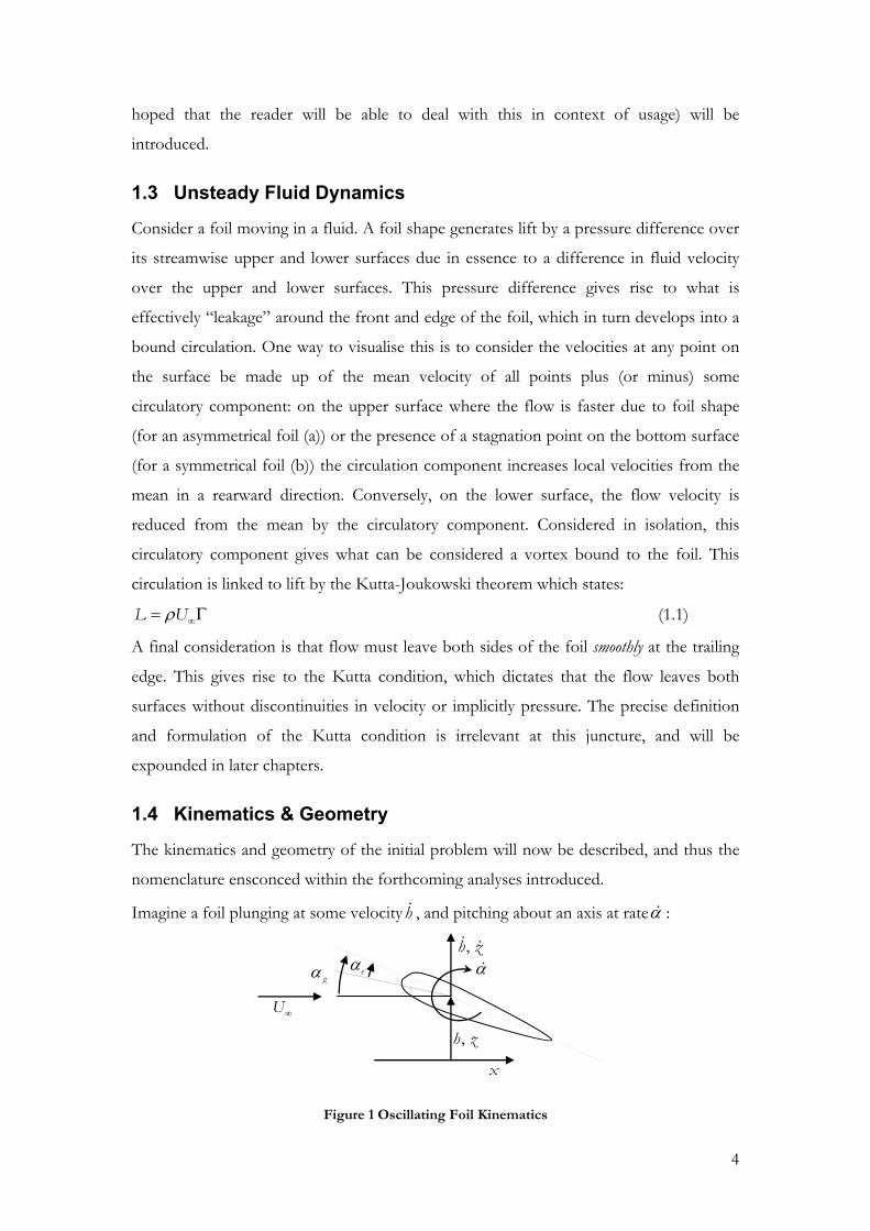
1.4 Kinematics & Geometry

The kinematics and geometry of the initial problem will now be described, and thus the

nomenclature ensconced within the forthcoming analyses introduced.

Imagine a foil plunging at some velocityh , and pitching about an axis at rateα :

gα eα α

,h z

,h z

U∞

x

Figure 1 Oscillating Foil Kinematics

5

Since the lift equation has dependence on angle of attack we may write for small angles

212 l g

hL U cCUα

ρ α∞∞

= −

(1.2)

This is the quasi-steady approximation. The term in parenthesis represents the reduction

in pitch due to the motion of the foil and results in the effective angle of attack eα .

Now consider a foil that is at an angle of zero to the incident flow at time t=0, which at

time t=t undergoes a step change in angle of attack to α. At t=0 there is no lift (no

circulation), but as soon as there is flow asymmetry about the foil, circulation is induced

and lift is generated. According to the Helmholtz circulation theorem the net circulation

in a control volume must remain constant (the net circulation must remain zero) and as

such vortices are shed by the foil in order to conserve angular momentum. If the Kutta

condition is applied at the trailing edge, then theoretically (adopting the assumptions

implicit in the Kutta condition) this would be the only place for the shed vortex to form.

The vortex is formed at t=t and thereafter is convected downstream. As it moves away

from the foil, it exerts a downwash over the surface of the foil, which effectively reduces

the angle of attack. As it convects into the farfield, the downwash decreases

asymptotically over time. Thus, the foils aerodynamic forces are

( ) ( )( ),b wL t U f tρ ∞= Γ − Γ (1.3)

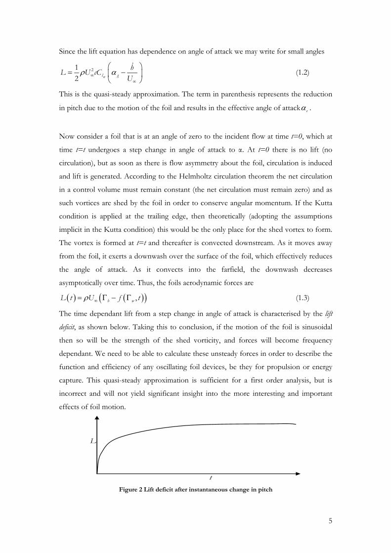
The time dependant lift from a step change in angle of attack is characterised by the lift

deficit, as shown below. Taking this to conclusion, if the motion of the foil is sinusoidal

then so will be the strength of the shed vorticity, and forces will become frequency

dependant. We need to be able to calculate these unsteady forces in order to describe the

function and efficiency of any oscillating foil devices, be they for propulsion or energy

capture. This quasi-steady approximation is sufficient for a first order analysis, but is

incorrect and will not yield significant insight into the more interesting and important

effects of foil motion.

L

t Figure 2 Lift deficit after instantaneous change in pitch

6

( )0, 0, 0 0t Lα= = = Γ =

0, 0, 0,b w bt L> > Γ > Γ = −Γ

, ,ss b sst L L→ ∞ = Γ = Γ

Figure 3 Schematic of downwash after step change in incidence

An important definition is the phase angle between pitch and plunge. Assuming that the

surge motion is constant and equivalent to the incident freestream velocity, it is the phase

angle along with pitch that will determine whether the foil will generate thrust or drag –

thrust generation corresponds to locomotion, drag corresponds to power capture. The

incidence could be above or below an intermediate angle whereby the foil was feathered,

doing no useful work, but it is the phase angle which determined whether useful work is

being done, bearing in mind that power is the product of force and velocity viz:

Figure 4 Phase angle (reprinted from Jones et al 1997)

In Figure 1 the foil is shown with 2 degrees of freedom. If the foil moves sinusoidally in

pitch, plunge (and surge if we use 3 DOFs) then the wake can develop into a fairly

complex structure, known as a von Kármán vortex street (Munsen (1998)), shaped by the

harmonic motion of the foil and the interaction between different regions of wake. Since

the lift, or strictly the pressure on the foil surface is influenced by the wake, it is useful to

define some quanta by which similar systems may be compared. These are reduced

frequency when considering the foil motion cUk ω

∞= , and the Strouhal number for

U∞

U∞

7

definition of the wake as well as foil kinematics 0h cUSt ω

∞= (NB 0h is the amplitude of

oscillation in terms of the foil chord).

Returning to the reciprocal relation between the motion of the foil and the vorticity in

the wake, all the main points required for an analysis of an oscillating foil for marine

energy capture have been introduced. Again turning to nature, examples of this type of

arrangement are more common that may be immediately thought. Any system where

there is interplay between some structural stiffness and the effect of shed vorticity will

show oscillating foil motion. From that of Venetian blinds, the fluttering of a flag to the

collapse of the Tacoma Narrows Bridge, coupling between structural and aerodynamic

modes is common and, where the body is structurally stiff, frequently catastrophic if the

shedding frequency comes close to the natural frequency of vibration. The problem may

now be specified as follows. For an oscillating foil device to succeed, it must generate the

maximum power from the flow while operating away from regions where coupling

between fluid dynamic forcing and system elastic modes becomes problematic. That said

if the interaction can be managed there is every likelihood that an unstable relationship

will generate the most power.

This thesis is primarily concerned with marine current power capture, so noting that

power captured by a device moving in the pitch, plunge and surge degrees of freedom,

can be written:

α= +P Lh M (1.4)

It is obvious that power capture will vary harmonically and so in quantifying power

output the power must be time averaged over an integer number of cycles. Maximising

power capture then depends on some optimising the variables within the constraints of

hydroelastic cross-coupling and reasonable structural limits, as well as maximising the

power take off portion of the stroke. In other words stroke length must be optimised so

that there is a reasonable period of generation during the cycle, with a long, high lift

stroke being optimal, and minimal forcing required pitching the foil against the fluid

forces. Additionally, it becomes advantageous to have the foil set to an optimum angle of

attack for most or the entire stroke. This means that there shall be significant shed

vorticity as the foil changes angle at either end of the stroke, and the influence of the

strong vorticity on the foil, structure and environment can become a concern. Clearly

there is scope for optimising the cycle within these parameters, and as such the rationale

for the study is defined by the following objectives.

8

1.5 Aims & Objectives of the Current Work

The aims of the current work can be broken down in the following manner:

Part A

Identify parameters related to the performance of oscillating foil systems and establish

their relative importance

Work with these parameters to optimise the power cycle for a typical system

Part B

Use the knowledge gained in part A to investigate an exemplar system specifically in

terms of a requirement for a simplistic control strategy for angle of attack

1.6 Outline of the Thesis

In order to meet the objectives stated above the following work is split necessarily into 7

chapters, and into 2 parts depending on restrictions on information contained within:

Part A:

In Chapter 2 a literature review is presented outlining in more depth the use of flapping

foils in nature; a review of the hydro/aerodynamics and hydroaeroelastic principles and

methods for dealing with oscillating foils; some discussion about wake formation; and a

summary of the Stingray project

In Chapter 3 the theoretical basis for computational modelling of oscillating foils is

expanded and an unsteady panel method model is developed. This method includes wake

development and allows the aerodynamic characteristics of the system to be determined

for arbitrary motion of the foil

In Chapter 4 the unsteady panel method is verified and parameter identification is done

in order to establish key variables.

Part B:

In Chapter 5 a mathematical model of the exemplar device is developed and the device

performance analysed using a Matlab model. Key variables are evaluated in terms of their

effect on device performance.

In Chapter 6 the changeover section of the device developed in Chapter 5 is dealt with in

detail, and observations from the computational models are reported.

In Chapter 7 the major conclusions from the study are presented, and suggestions for

future development of the model and research are made.

9

Ch. 2 Introduction to Oscillating Foils

This chapter intends to extend on the introduction of flapping foils for locomotion in

nature and by man and review the hydro-aerodynamic performance of such devices for

thrust and power production. Potential flow will be introduced, historical analytical

framework will be reviewed and discussion of the wake structure behind an oscillating

foil will provide a segue into the current unsteady method described in the sequel.

Finally, a brief synopsis of the Stingray project will be presented in order to provide

insight into the practical difficulties and intricacies of actual device performance.

2.1 Flapping Foil Locomotion

Aeons of evolution have gone into perfecting the locomotion of birds, insects and the

fishes, so it is not surprising that man is looking closely at their design and configuration

in an effort to enhance the development of flapping foil devices. That is not to say that

all creatures are equally adept, but it is clear as to which are successful and should be

studied. Starlings can travel at 120 body lengths per second, dolphins and fast fish can

achieve up past 8 body lengths per second through water. A Boeing 747 flying at top speed

(967kph – length 70.67m) achieves 3.8 body lengths per second and although fighter jets

fare far better (38 body lengths per second for a RAF Tornado at full speed at 40,000ft)

they cannot compete with starlings and definitely not with some insects (desert locust:

180 body lengths per second).

Biomimetics is the attempt by engineers to mimic successful evolutionary design, and to

be useful is not straight copying, but more an appraisal of the design itself in terms of the

principles of operation. Thus various studies have drawn out the modes of operation for

successful species, and similarities have been discovered. Rhozhdestvensky and Ryzhov

(2003) present a thorough review of flapping wing propulsors both natural and manmade

and present feature lists of flight and swimming modes of creatures. Generally in cases

where adaptation for speed exists a propensity for exploitation of an artificially generated

unsteady, vortex generated flow is found. As mentioned in the introduction insects such

as bees can generate exceedingly high lift coefficients by utilising energy in shed vortices

from the wing leading edge, and in the wake shed by the fore-wings (Ansari et al

(2006,2006), Guglielmini (2004)) . Favourable interaction between leading and trailing

edge vortex wakes leads to high propulsive efficiencies. Birds exhibit a similar tendency,

10

but can operate at significantly higher Reynolds numbers where the inertial effects

dominate (insects: 100-104; birds: 104-106). Bird flight is characterised by large, complex

interactive wake formation from the wings and body, the aerodynamic study of which is

in its infancy due to a high level of physiological and morphological complication,

however Hedenström (2002) indicates that the influence of wake formation coupled with

optimally evolved flying styles and continually adaptable geometry (which has drag

reduction implications) have a significant role in the success of bird flight. As an aside,

there is evidence that what may have been vestigial thumbs apparent on some bird wings

(known as “bastard wings” or alulae) act to generate significant lift increases at low

speed, operating in a similar manner to high lift devices on aircraft. While the net effect is

to increase the camber of the wing, a side effect is that the main wing operating in the

wake of the alulae will experience a predominantly circulatory flow, the effects of which

are to energise the boundary layer on the main wing, delaying stall, and interaction

between the vortices shed from both wing structures (Greenblatt (2000)). Cheng et al

(2001) using a 3D CFD analysis on fish, found a similar interaction between

dorsal/ventral fins and the tail, leading to a very precise pattern of vorticity shed from

the middle of the tail. The peculiarity was that since the wake was effectively shed from a

location at the middle of the tail, the characteristics approached that of a 2D wake, and

losses due to tip vortices where minimal. In both cases it is the turbulence in the

impinging stream which is causative, and one might suspect that a similar situation would

exist if an oscillating foil device is positioned in a turbulent tidal stream, specifically in the

shear layer close to the seabed.

Large fish and cetaceans also operate at these higher Reynolds numbers (104-108).

Similitude analysis using Strouhal number indicates that high speed marine creatures are

found to operate within the range 0.281<St<0.407 with the mean, 0.36, typical for most

creatures. A sensitivity study by Tryantafyllou et al (1993) found the wake generated by

an oscillating foil acted to selectively amplify forcing at that frequency, a kind of fluid

resonance, and the non-dimensional frequency of maximum amplification in terms of St

was 0.25 to 0.35. Since this frequency range provided maximum amplification, the

efficiency of operation in this regime would also be maximal. It was then shown that

high speed fishes of many species, and cetaceans were found to operate within this

optimal frequency band. It is not surprising, seeing that (intuitively) the most important

parameters have been found to be dimensional speed, frequency and amplitude of

11

oscillation, Strouhal number similitude will provide guidance for choice of regime for

designing flapping foil propulsors.

The analysis by Lighthill (1969, 1970) presents a compendium of aquatic locomotion for

marine creatures. Amongst others he has quantified and described the motion of the

lunate tailed tuniform and carangiform species (this is a phenotypical as oppose to a

claddistic description, a bit like lumping frogs and trees together because they are both

green) to which sharks and dolphins belong, noting fishlike motion is a reaction of

hydrodynamic forces composed of a reactive component as well as a momentum

addition due to vortex shedding and that in these species the wave like bending motions

required to “push” the water rearwards had evolved to occur at the tail end. This led to

an increase in the size of the fish tail, and as speed of locomotion increases so too does

the range of motion of the tail and flexibility of the body, with tail motion corresponding

to effective manmade flapping propulsion devices. The net flow behind the fish is in the

form of a jet, or a momentum surplus but under the harmonic excitation by the tail it

degenerates into a staggered array of vortices (a von Kármán vortex street). However, the

flow does form a dynamic equilibrium with a mean momentum surfeit across the cycle

and according to experimental work by Koochesfahani (1989) if two vortices are shed

per cycle (reverse Kármán street) then the wake is stable and has average properties alike

a simple jet.

In work carried out based on analysing video footage of dolphin swimming in the wild,

the flapping motion of the tail appears to approximate a sinusoid, and it is through

precise control of the fin induced angle of attack that maximum thrust can be generated.

The induced angle of attack was found to not exceed 10°, and the flow remained

attached (separation appears to cause some physical pain to the animal, as well as

detrimental performance). Observations indicate that the phase angle between pitch and

plunge oscillations is 2πφ = lagging and so precise is the control of the dolphins tail, that

even though the plunge amplitude can be severe the dolphin maintains the optimum

angle of attack through the vast majority of the cycle, with putting the fin over taking is

in the region of 0.02-0.16s, minimising or removing altogether deceleration of the animal

though the water. Since propulsors and energy extraction devices are likely to operate

within the same Reynolds number regime, it is instructive to analyse the motion of

dolphin size hydrobionts.

The use of flapping foils for vehicle propulsion is not a new idea. Leonardo da Vinci

proposed an ornithopter c1485, and early aviation pioneers looked to birds when

12

designing their (doomed) aircraft in the 19th century. The problem was that the weight

and complexity of man designed flapping wing propulsors and the lack of a suitable

power plant prevented any of these designs leaving the ground and the idea was

abandoned until work during the Second World War by Schmidt indicated that oscillating

wings were a viable propulsors for marine vessels.

In 1973 the Arab oil producing states set up an embargo, refusing to sell oil or petroleum

to any nations who supported the Israelis in the Yom Kippur war, and as such

industrialised nations dependant on oil faced an energy crisis. In response, fuel prices

escalated well above inflation and a raft of measures was introduced to curb demand and

seek out alternatives. This gave a boost to the renewables industry, with the US and other

countries beginning to seriously investigate wind, solar and biomass sources.

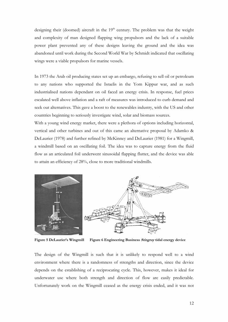
With a young wind energy market, there were a plethora of options including horizontal,

vertical and other turbines and out of this came an alternative proposal by Adamko &

DeLaurier (1978) and further refined by McKinney and DeLaurier (1981) for a Wingmill,

a windmill based on an oscillating foil. The idea was to capture energy from the fluid

flow as an articulated foil underwent sinusoidal flapping flutter, and the device was able

to attain an efficiency of 28%, close to more traditional windmills.

Figure 5 DeLaurier’s Wingmill Figure 6 Engineering Business Stingray tidal energy device

The design of the Wingmill is such that it is unlikely to respond well to a wind

environment where there is a randomness of strengths and direction, since the device

depends on the establishing of a reciprocating cycle. This, however, makes it ideal for

underwater use where both strength and direction of flow are easily predictable.

Unfortunately work on the Wingmill ceased as the energy crisis ended, and it was not

13

until 1997 when the Engineering Business set up the Stingray programme (DTI 2002,

2003, 2005) that the concept received any real consideration. The prototype stingray

device was tested off the Shetland isles in 2002 and 2003. The Stingray device was in

principle a large, controlled hydrofoil mounted on an arm whose motion drove a set of 6

hydraulic generators and whose pitch was controlled by sophisticated systems. The blade

itself was a relatively unsophisticated NACA0015 section with an area of 172m2 and a

chord of 3m, and was set to oscillate through 35° whilst maintaining an optimum angle

of attack to the flow. The 11m arm was secured to a massive base unit mounted on the

seabed and power was obtained through hydraulics operating between the arm and the

base.

The basic outcome of the project was that the device performed reasonably well,

generating at 122kW with a flow speed of 2.25ms-1, with decent results at lower speeds.

The problems came with the complexity and cost of the device. Control systems were

very complex, in order to maximise the power output – it required many interacting

sensors and actuators, along with several computerised control software systems to

maintain optimality – and this fed into a general issue with unreliability which plagued its

performance. An additional issue with the Stingray was the shedding of massive vortices

at the point where the foil was put over. Finally, the device was shelved as the

Engineering Business due to financial concerns.

2.2 Historical Mathematical Analysis

Wing flutter is a well known phenomenon in the hydro/aeronautical industries

concerning a coupling between the pitch and/or plunge motion of a wing section with

structural elasticity and nominally there exist two types: pure pitching, and coupled

flapping. Flutter is of interest as it is energy extraction from the flow which provides the

motion, which in pitching only flutter is relatively benign, but in coupled flapping flutter

structural elasticity and periodic forcing can very quickly lead to catastrophic failure.

For a thin aerofoil oscillating harmonically in incompressible flow there is an exact

solution to the unsteady lift due to the seminal work of Theodorsen (1935), and this

constitutes the classic American analysis. He considered a flat plate in incompressible

potential flow with the Kutta condition and infinitesimal aerofoil motions.

14

b− b+

← ab → bdsγ wdsγ

,x s EA

z

Figure 7 Theodorsen nomenclature

The upwash due to aerofoil motion is, at point x:

( )abxhU −++= αω αα (2.1)

From the Biot-Savart lay the upwash due to bound vorticity is

12

b bb b

dsx sγω

π −=

−∫ (2.2)

Similarly, the downwash from the shed wake vorticity is

12

wb

dsx sγλ

π∞

=−∫ (2.3)

Using the unsteady linearised Bernoulli equation (3.17) and boundary conditions

Theodorsen used these expressions to derive an integral equation for the bound vorticity

and hence lift

2 2 wb

C Q

wb

s dss bL Ls b dss b

γ

γ

∞

∞

−=+−

∫

∫ (2.4)

It should be noted that the integral equation is evaluated over the whole wake thus the

lift is a function of the entire history of the aerofoil motions. Given that during flutter

the aerofoil oscillates harmonically, the wake vorticity is also harmonic, so:

{ }( )exp sw w Uj tγ γ ω= − (2.5)

Where the terms in curly brackets represent wake convection.

This results in the following expression:

( ) QC LkCL = (2.6)

Where Ubk ω= is the reduced frequency and

( )( )

( )

∞

∞

−−=+

−−

∫

∫

21

1

exp11 exp1

s jks dssC ks jks dss

(2.7)

15

The effect of the wake is to multiply the quasi-steady lift by a function C(k) which is

frequency dependant. The function C(k) turns out to have a compact solution composed

of Bessel functions

( )( ) ( )

( ) ( ) ( ) ( )=

+

21

2 20 1

H jkC k

H jk H jk (2.8)

Where ( )2nH is the modified Bessel function of the second kind of ordern . C(k) is the

Theodorsen lift deficiency function and means that the unsteady lift is a complex number

at any frequency k.

( ) ( ) ( )= +C k F k jG k (2.9)

The lift deficiency function basically scales the quasi-steady approximation to include the

effects of the change in foil circulation with respect to the dynamic influence of the

wake. The result is that the wake has a delaying effect on circulatory lift (the phase is

altered) and so if the foil is oscillating with some frequency ω there will be a phase lag

such that

( ) ( )sinC CL t L tω φ= + (2.10)

The simplifying assumptions of Theodorsen include a planar wake, where the wake is

simply a straight line in the plane of symmetry and does not deform, and that the foil is

an infinitesimally thin flat plate. However subsequent work by, amongst others, Jones &

Platzer (1997) indicates that the drop in accuracy does not significantly affect the results,

and does not mask principle characteristics – at least for a certain range of k.

The Theodorsen function was used by Garrick (1937) in his approach to the flapping

wing propulsion problem. He used a linear analysis which extended that of Theodorsen

to include plunge, but is still based on Theodorsen’s original approximations. The results

of Garrick’s work include the time dependant aerodynamic forces on the foil, and thus

allow calculation of time dependant thrust and power. Further work by Garrick extended

the usefulness of this by formulating expressions for time dependant forces on a foil

undergoing flapping motion with arbitrary parameters. This significantly extended the

generality of the resulting expressions, which are identical to those obtained by Lighthill

(1970) after some manipulation. Lighthill’s work was based on the slender swimming fish

propulsion by a semi-lunate fin and was derived from energy considerations in small

amplitude motion assuming a constant phase difference for pitching (leading 2πφ = )

versus plunging motion, limiting generality. Garrick showed that in all pure plunging

motion a foil was capable of generating thrust with efficiencies that approached unity as

16

frequency tended to zero, and asymptotes to 0.5 as frequency rose. Additionally, Garrick

demonstrated that thrust is approximately proportional to the square of the frequency –

this means that at high propulsive efficiency only limited thrust is produced, meaning

that large flapping appendages would be required to achieve significant thrust at

reasonable frequencies, and as such interest waned and alternative means of propulsion

were sought (the historical context is significant).

As an aside, the later work by Schmidt (1942) indicated that low thrust from a plunging

foil could be increased by having a stationary foil placed behind it in the oscillating wake.

As an engineering compromise the plunging motion was changed to a circular one, and a

device as such was used to power boats. The principle is very similar to that of the Voith

propeller (strictly a pump) and the inverse of the Darreius turbine.

Jones & Platzer (1996) compared experimental and numerical results in an investigation

of wake structures behind plunging aerofoils. Using a water tunnel and a computational

code similar to that described herein the shed wake from a foil was visualised under a

variety of thrust and drag producing situations. In these conditions there is a mean

velocity or momentum surplus or deficit on the centreline of oscillation in the fluid

downstream of the foil, a direct and cumulative result of the vortical structures found in

the wake influence over fluids velocity. Since the Theodorsen method assumes a planar

wake with sinusoidal vorticity strength along its length, the effects of this assumption

were one of the motivations for the study. Jones & Platzer (1997) later demonstrated that

at low k agreement between the linear Garrick method and the numerical and

experimental results is good, but diminished as k increased, since the wake was free to

deform non-linearly, and as the von Kármán vortex roll up occurred, propulsive

efficiency dropped. This could have significant bearing on the efficiency of an oscillating

foil power generator, as increasing energy lost to the wake could have serious detrimental

feedback effects as well as the obvious efficacy implications. Indeed, the investigation

indicated that the non-linear deformation of the wake was responsible for almost all of

the difference between the linear and computational methodologies. Finally, an inclusion

of a drag computation (by boundary layer expansion) indicated that losses due to

viscosity were almost linear, and as such the increased accuracy afforded by the

deforming wake method, and the low computational cost associated with the inviscid

method allows rapid computation and simple modelling.

17

2.3 The von Kármán Vortex Street & Strouhal Number Dependence

A fundamental dimensionless parameter in flows displaying an unsteady and oscillatory

fluid motion is the Strouhal number, St. This relates the unsteady fluid forces to the

convective ones, and offers at the very least a measure of the velocity due to flapping in

terms of the “forward” motion of the foil through the fluid. Based on plunge amplitude

it is also useful in predicting whether a flapping foil is likely to produce thrust or drag

since at the point where the foil experiences (approximately) zero equivalent angle of

attack throughout the cycle and is feathered, if the phase between pitch and plunge is

2π lagging, the maximum geometric incidence excursion will be given by ( )1tan Stα −∆ =

and any pitch setting below this will theoretically provide thrust (or at least will require

power input) and any pitch setting above should provide net power output. The Strouhal

is classically defined in terms of the frequency of vortex shedding, and the length scale

term is the vertical distance between the shed vortices. In this investigation, for

simplicity, the Strouhal number length scale is approximated as the plunge amplitude.

The stability of the flow may be hinted to by the Strouhal number: for low St it is

possible to have a small ratio of plunge amplitude and frequency to freestream velocity

and in either of these cases the wake induced velocity on the foil is likely to be negligible.

However, it is possible to have a low St with small plunge amplitude and a high

frequency and as such St cannot provide a complete description of flow characteristics –

this is where the reduced frequency k comes in.

At certain frequencies, the flow can become sufficiently unstable that asymmetric vortex

shedding can occur. This gives rise to the famous Kármán vortex street, where shed

vortices form opposing pairs, invaginating the wake. As hinted this is only likely to be

seen at Strouhal numbers with reduced frequencies above a certain value, below which

the wake vorticity is convected away before it interacts. Vortex wake structure has been

studied experimentally by, amongst others, Katz and Weihls (1978) and numerically by

Jones et al (several times, e.g. 1997), but it was von Kármán who did the ground work,

offering a theory describing the thrust and drag production of the wake, based on the

position and orientation of the vortices (von Kármán and Burgers 1943). Their work

built on previous work by Knoller and Betz, who independently arrived at the same

explanation for the thrust production of flapping wings in the early 1900s.

18

The wake may take on of three meta-stable forms: thrust producing where there is a

momentum gain or “jet” formed by the average fluid velocity across the wake; neutral

where there is no net change in fluid momentum and drag producing, where there is a

momentum deficit in the average fluid properties. From energy considerations, it is not

possible to have a thrust producing wake without doing work to the flow in moving the

foil, and it is unlikely that a neutral wake may be formed in the same way (this follows

from the second law of thermodynamics which essentially requires input energy for the

vortical dissipation). It is probable that a drag producing wake may be created, even with

energy input if the foil is not set up correctly. However, a drag producing wake can also

indicate that work is being done to the foil by the fluid. The three wake setups are shown

in the following photographs:

Figure 8 Drag indicative Kármán street, after Jones et al (1996)

Drag indicative vortex wake, characterised by upstream direction of mushroom shaped

vertical structures, and clockwise rotation of upper vortices. Next is the neutral wake.

Note the mushrooms have a cross stream direction, and additionally that there is an

alternating series of eddies lying on the centreline of the foil motion.

Figure 9 Neutral vortex street, after Jones et al (1996)

19

Figure 10 Thrust indicative Kármán street, after Jones et al (1996)

The thrust producing wake shows eddies of sign minus that of the drag producing wake,

and also a downstream orientation for the wake structures. The eddies have formed pairs

of opposing rotating vortices, however unlike the case of the drag producing wake,

where it is clear that at the centreline location the eddies conspire to mush the fluid

upstream, for the thrust producing wake it can be seen that the effect of the vortices at

the centreline is to push the fluid downstream.

20

Ch. 3 Development of the Fluid Dynamics Model

3.1 Potential Flow

The approach of Basu and Hancock is employed in this investigation to model the

unsteady fluid dynamic effects on the oscillating foil, and is itself based on the method of

Hess and Smith for modelling a steady flow foil. The method predates modern

computers and as such relies on a very specific set of approximations and assumptions

for modelling the fluid mechanics of the situation, which now, in combination with

reasonable computing power allow solutions to be calculated with some rapidity. It is

also what may be considered a benchmark method, used widely with success, and the

method is itself fairly intuitive. The Hess and Smith method relies on potential flow and

here the underlying principles will be introduced.

In planar potential flow it is assumed that the flow has only velocity components in the

x-z plane and is incompressible. In this case the mass continuity equation reduces to:

0∇ ⋅ =V (3.1)

Or

0u wx z

∂ ∂+ =

∂ ∂ (3.2)

And by introducing a potential stream function ψ we can relate the velocities as

ψ∂=

∂u

y ψ∂

=∂

wx

(3.3)

So by describing the flow in terms of ψ it can be seen for any arbitrary ψ that mass

continuity will be satisfied. An additional advantage is that lines of constant ψ are

streamlines – that is that the flow along such lines is parallel to the lines, with no normal

component. With an additional assumption of irrotational flow it is simple to analyse

flows which satisfy these assumptions. By introducing another term, the velocity

potential φ asφ( , , )x z t , which is a scalar, we can define the velocity components as

φ∂=

∂u

x φ∂

=∂

wy

(3.4)

Which when substituted into the definition of an irrotational fluid

∇× =12 V 0 (3.5)

21

can be written in vector form as

φ= ∇ ⋅V (3.6)

For 2D flow we now have equations (3.1) and (3.6) which are respectively consequences

of mass continuity and irrotationality and can be found by reduction of Euler’s equations

of fluid motion. They can be combined as

φ∇ =2 0 (3.7)

or in Cartesian coordinates

φ φ∂ ∂+ =

∂ ∂

2 2

2 2 0x z

(3.8)

This is the Laplace equation and provides the theoretical underpinning for the

subsequent analysis. A more complete treatment of the above derivation can be found in

e.g. Munson (1998). The advantages of such an approach is that the velocity (and

pressure) may be calculated at any point in the flow field using (3.4), and as it is a linear

partial differential equation complex flow fields may be built up by superposition of

simple solutions, i.e. if φ φ φ…21 , , n are solutions to (3.7) then so too is

φ φ φ φ= + + +…3 21 n .

The simple solutions that the models used in this thesis are built from are uniform flow,

source/sink and vortex potentials, and their individual solutions are presented here

without derivation: Table 1 Flow solutions including polar and Cartesian components of induced velocities.

Freestream

∞U

α

x

z

'z 'x ''

U xU y

φψ

∞

∞

==

Strength: ∞U Sign according to coordinate frame

cossin

u Uw U

αα

∞ ∞

∞ ∞

==

Point vortex

x

z

r

vθ

θ

φ θψ

= Γ= −Γ ln r

Strength: Γ Sign +ve CCW

θ

θπ

θπ

Γ=−Γ

=

Γ=

sin2cos2

r

v

v

v

ur

wr

Point source/sink x

z

r

rv

θ

σφπ

σθψπ

=

=

ln2

2

r Strength:σ Sign +ve radiating outwards (source) -ve inwards (sink)

σπ

σ θπ

σ θπ

=

=

=

24

cos2sin2

r r

s

s

v

ur

wr

22

As is apparent when considering the vortex potential, there is a singularity at the vortex

centre where the induced velocity will become infinite and where the calculation calls for

a computation of induced velocity at some small r the induced velocities will be

artificially high – this issue is dealt with by using Rankine cores in the unsteady panel

method and is discussed in the sequel.

3.2 Assumptions

The assumptions used are as follows:

• steady flow

• inviscid flow

• incompressible flow

• irrotational flow

The assumption of steady flow is only valid in the case of the steady solution panel

method, and the effects of unsteady flow are dealt with in the use of the unsteady

Bernoulli equation when the unsteady panel method is presented. The assumption of

inviscid flow requires that there is no viscous shearing stresses on the surface of the foil,

or within the fluid and is tied in with the assumption of irrotationality inasmuch as it only

requires that the individual fluid “packets” are irrotational and do not deform – the flow

itself can rotate as long as the motion is made up only of translation of the packets – and

is only really crucial in boundary layers where viscous effects dominate. Since the foil is

likely to operate in high Reynolds number flow where inertial effects dominate (except in

boundary layers) boundary layers can be assumed to be infinitesimally thin, with a caveat,

and Reynolds number is infinite. The caveat is of course in the situation where the

boundary layer grows at stall and as such in this method there is no treatment of stall at

all, and the flow is considered attached at all times. Obviously this is unrealistic and so

care must be taken when accepting results for aerofoils operating in conditions where

stall and separation occur, for example at effective angles of attack higher than

approximately 15 degrees.

23

Using the definitions and requirements of potential flow introduced above it is possible

to generate a fluid mechanics model of the oscillating foil from which the hydrodynamic

forces may be calculated including unsteady effects. The first step is the breakdown of

the problem and generation of general boundary conditions suitable for a steady state

analysis. This is then extended to the unsteady computation.

3.3 Steady Model

Recall that in potential flow it is possible to generate flow solutions by a linear solution of

Laplace’s equation, simply by the addition of the various singularities and flow

characteristics within the domain. This allows us to specify certain boundary conditions

to achieve a numerical computation of the fluid domain. Thus if we wish to model a solid

(read impermeable) object in a moving fluid, we would model the fluid using the

freestream identity and the boundary conditions required to satisfy impermeability by a

distribution of elemental solutions (vortices, sources, etc). The linear nature allows a

systematic evaluation to proceed by allowing a simultaneous solution to the entire

domain. Unfortunately the nature of the Laplace equation ( 2 0φ∇ = ) requires additional

conditions to be applied if the solution is to be unique, and this is accomplished in the

case of a foil by using the Kutta condition, of which more later.

Thus for an aerofoil in steady flow the problem is solved as follows:

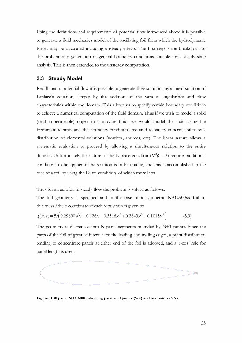
The foil geometry is specified and in the case of a symmetric NACA00xx foil of

thickness t the z coordinate at each x position is given by

( )2 3 4( , ) 5 0.29690 0.126 0.3516 0.2843 0.1015z x t t x x x x x= − − + − (3.9)

The geometry is discretised into N panel segments bounded by N+1 points. Since the

parts of the foil of greatest interest are the leading and trailing edges, a point distribution

tending to concentrate panels at either end of the foil is adopted, and a 1-cos2 rule for

panel length is used.

Figure 11 30 panel NACA0015 showing panel end points (‘o’s) and midpoints (‘x’s).

24

0 0.1 0.2 0.3 0.4 0.5 0.6 0.7 0.8 0.9 10

0.1

0.2

0.3

0.4

0.5

0.6

0.7

0.8

0.9

1

fz

fx

iθ

ˆ in ˆ iτ

Incident flow

iU

i th panel control point

Figure 12 1-cos2 distribution of panel length

along foil chord

Figure 13 Situation at the i th panel showing

nomenclature

The current method numbers these panels working clockwise from the trailing edge. At

each panel the requirement of impermeability provides a boundary condition of zero

normal flow, thus for the i th panel located between the i th and i+1st nodes we have

equation (3.10) with the nomenclature as shown in Figure 13. For each panel the

condition of zero normal flow is evaluated at a control point located at the midpoint of

that panel, and the method is consistent with the Hess & Smith approach.

ˆ cos sin 0i i i i i iu wθ θ⋅ = − + =U n (3.10)

Working in global coordinates if we now assume that there is an elemental solution of

strength iΦ placed on each panel we can now write the zero normal flow equation in

terms of the influence of the elemental solutions at each panel on the control point of

the i th panel

1

1

1 1

ˆ cos sin 0

N

j ijj

i N

j ijj

N N

i i j ij i j ij ij j

u

w

u wθ θ

=

∞

=

= =

Φ = +

Φ

∴ ⋅ = − Φ + Φ =

∑

∑

∑ ∑

U U

U n

(3.11)

Where the terms uij, and wij are the normalised (eg their value is multiplied by the

elemental solution strength to give the actual velocity perturbation) perturbation

velocities acting on the i th panel control point due to the elemental solution on the j th

panel. We now have a system of N equations for flow tangency with N unknowns for the

elemental solutions. At this point it is apparent that there are a large number of potential

solutions which satisfy the zero normal flow condition, and consequentially the Kutta

condition is required to calculate the specific unique solution. The current method

specifies that on each panel there is a distributed source potential, whose strength σ is

25

constant along the panel, but may vary between panels, and the Kutta condition enforced

by a distributed vorticity potential whose strength γ is constant over every panel on the

foil. The vorticity ensures that the flow leaves the trailing edge smoothly by stipulating

that the velocity is finite and continuous at the TE, done by specifying equal velocities on

the panels either side of the TE. However this is an assumption that greatly affects the

flow conditions around the foil and whose validity decreases rapidly as the length of the

TE panels increases and if the TE panels are of different length. These are avoided by

having a symmetric foil and having especially small TE panel lengths which are a natural

product of the 1-cos2 panel length distribution.

There are now N equations for zero normal flow and a Kutta condition equation, and

N+1 unknowns for the distributed source strength at each panel, and the distributed

vorticity strength over all the panels. Equation (3.11) can now be written as follows, again

in terms of perturbation velocities due to the source and vorticity distributions.

1 1

1 1

cosˆ 0

sin

ij ij

ij ij

N N

j s vj j i

i i N Ni

j s vj j

u u

w w

σ γθ

θσ γ

= =

= =

+ − ⋅ = = +

∑ ∑

∑ ∑U n (3.12)

Calculation of the perturbation velocities for distributed source and vorticity strengths is

based on the singularity values introduced in Table 1.

In order to calculate the influence of the distributed elements it is convenient to work in

a panel based reference frame, related to the foil based reference frame by transformation

T1 and to the global reference frame by T2T1. In the reference frame of the j th panel, and

with the panel lying along the x*-axis the influence of a source or vorticity distribution of

unit strength along the j th panel on the control point of the i th panel is found by

integrating the singularity influence in x* as follows, with the closed form solution

coming from tables.

( )

( )

( )

( )

2

2

2

2

120

20

20

120

1 1 ln2 2

12 2

12 2

1 ln2

j

ij

j

ij

j

ij

j

ij

length ijs

ij

length ijs

length ijv

length ijv

ij

rx tu dtrx t z

zw dtx t z

yu dtx t z

rx tw dtrx t z

π π

βπ π

βπ π

π

∗+∗

∗ ∗

∗∗

∗ ∗

∗∗

∗ ∗

∗+∗

∗ ∗

−= = −

− +

= =− +

= − =− +

−= − =

− +

∫

∫

∫

∫

(3.13)

26

With subscript ‘s’ or ‘v’ indicating singularity type. In solving these with limits, they may

be interpreted as a radius and an angle, with rij being the distance from the j th panel end

point to point i, the i th panel’s control point, and similarly for 1ijr + . The term ijβ is the

angle subtended at point i by the j th panel. A final note on the influence of a panel on

itself: here the value of iiβ depends on from which side you approach the panel. Since it

is the exterior problem which is of interest, all iiβ terms are identicallyπ .

The system of equations can now be recast into matrix form by introduction of influence

coefficients and transforming back into foil coordinates. The matrix is written in the

form Ax=b where the A terms are the influence coefficients, the x vector contains the

strengths of the source and vorticity distributions on the panels and the b terms are the

normal velocities seen at the control points at the panel centres not due to the panels

themselves. The following system of relations will illustrate the situation.

11

1 1 1

2

ˆ ˆ;

ˆi

N

ij j iN ij

sij vijij j i iN j i

sij vij

Ti i

A A b

u uA T A T

w w

b T

σ γ+=

∗ ∗

+∗ ∗

∞

+ =

= ⋅ = ⋅

= ⋅

∑

n n

U n

(3.14)

The Kutta condition terms are made up in a similar manner, but the flow tangential to

the last two panels is set equal and the AN+1,j terms are done only for the first and last

panel in order to determine the velocities at their midpoints. The expressions are similar

but the tangential unit vector is used.

1

1, 1, 1 11

1 2 1 2ˆ ˆN

N

N j j N N Nj

T TN N

A A b

b T T

σ γ+ + + +=

+ ∞ ∞

+ =

= ⋅ + ⋅

∑U τ U τ

(3.15)

The system of equations for the foil is now known and may now be solved for the

vorticity and source strengths around the foil. This is done (in the steady case) using

Gaussian elimination. Once the strengths are known, the flowfield may be calculated at

any point exterior to the foil using a linear addition of any of the relations above. The

pressure distribution on the foil is calculated by obtaining solutions over the surface of

the foil at the control points and using the steady Bernoulli equation – the aerodynamic

forces follow directly by integration. Since the boundary conditions state there is zero

normal velocity at the control points, it is implicit that the total velocity at any control

point on the foil surface will be tangential to the surface at that point, so there is no

27

approximation when using the following expression of the Bernoulli equation in

obtaining the pressure distribution. 2

21pC∞

= − iV

U (3.16)

To reiterate: the velocities at any point in the flowfield due to a panel’s source and

vorticity distribution is simply as given by the components in equation (3.13) and is

transformed into the global coordinate frame by the transforms linking panel and foil

and foil and inertially fixed frames of reference. The velocity due to all the panels making

up the foil is simply the accumulation of each panel’s contribution. This serves as

vindication of the simplicity inherent to the potential flow analysis – the computational

cost of the solution is many orders smaller than the cost of computing a similar solution

using more advanced equations, and while there are several limiting assumptions the

approximations are acceptable as long as the weaknesses of the method are appreciated

and the problems posed accordingly.

3.4 The Unsteady Panel Method

This follows the Basu and Hancock extension to the Hess and Smith approach above,

and requires some slight modification of the procedure to accommodate the non-linear

evolution of a wake and significant modification of the solving mechanism to

accommodate a timestep and unsteady effects. There is an addition of an element

attached to the trailing edge whose length and orientation is allowed to vary according to

the unsteady flow conditions and this introduces some additional non-linearity and

complicates matters somewhat. However the method still retains the elegance of the

steady method and is as follows.

3.4.1 Wake Evolution

As was explained above, a foil instantaneously moving through a fluid at some angle of

attack α will generate a bound circulation Γb which must be countered by a shed vortex

to maintain conservation of angular momentum – this is Kelvin’s circulation theorem –

and accordingly a foil moving arbitrarily through a fluid whose circulation is arbitrarily

changing according to its hydrodynamic incidence will release a continuous vortex sheet

in order to satisfy conservation. In order to model this with an unsteady panel code, at

28

each time step an individual vortex core of constant strength is deposited into the flow

and allowed to convect downstream according to the perturbation velocities acting on it

from the sources and vortexes on the foil, and the influence of the other shed vortices.

Note that at this point the position and strength of the newest shed wake vortex are

unresolved, and these are dealt with as follows.

Essentially the requirement of Kelvin’s circulation theorem is that the sum total of all

circulation in the flow is conserved, and so at each time step the shed vortex is of

strength equal to the difference between the current bound circulation strength on the

foil, and the bound circulation strength at the preceding time step. A possible scenario is

that the new vortex is then deposited into the flow immediately behind the trailing edge

of the foil at some point on the path travelled by the trailing edge - this assumes that the

flow leaves the foil at the TE and is an application of the Kutta condition. However, it is

argued by Maskel (in Basu and Hancock) that this approach is unacceptable, since

although the velocities are specified as being equal on the upper and lower surfaces, the

pressures are not. The unsteady Bernoulli equation is 2

2 2

21pCtφ

∞ ∞

∂= − −

∂iV

U U (3.17)

According to the unsteady Bernoulli equation, since there is a discontinuity in tφ∂

∂

associated with ∂Γ∂

bt at each time step, even with equal velocities on the upper and lower

surfaces there will be a finite pressure difference, which is physically incorrect. This gives

rise to the unsteady statement of the Kutta condition used in this method. It is simply

stated that the Kutta condition requires that there are equal velocities and equal pressures

required either side of the TE, which translates as zero loading across the TE elements

and there must be zero loading across the immediately shed vorticity in order that the

flow leaves the TE smoothly and is formulated in terms of the tangential flow either side

of the trailing edge.

( ) ( )2 2 11 1

1

ˆ ˆ 2 k kN Nk k

k kt t−

−

Γ − Γ⋅ = ⋅ +

−V τ V τ (3.18)

In order to ascertain the position for the new wake vortex, a small additional panel

element is attached to the trailing edge. The length of this panel kδ and its inclination

measured referring to the global x-axis wθ are functions of the flow conditions

calculated aft of the TE as part of the solution. This supplementary element functions as

29

a proto-vortex in place of a discrete shed vortex at the k th time step and is given a

vorticity per unit length according to the Kelvin condition.

1k w k kδ γ −= Γ − Γ (3.19)

This then seeds the series of shed vortices of strength k wδ γ which constitute the

downstream wake and, since there is no loading on the wake, convect according to the

resultant velocities calculated at their midpoints at each time step. The velocities induced

by the wake element and the wake vortices are accounted for in the calculation of the

right hand side of the unsteady equivalent to equation (3.14) in the following manner.

3.4.2 Formulation of the Unsteady Panel Method

Again we begin by defining the boundary conditions. As before, to ensure non-

permeability of the foil boundary a source and vorticity distribution is placed on each

panel, and the condition of zero normal flow is enforced at each control point (which

remain at the panel midpoints) by specifying the strength of the elemental solutions to

effectively cancel out the external velocities as seen at the control point. Thus the

external, incident flow velocities must be defined. In the steady state model, this was

simply the freestream velocity ∞U which was assumed to act parallel to the global x-axis

(thus having only an x-component) and which could be recalculated in the local panel

coordinate system by use of transforms T2T1. The external velocity must now be

recalculated to include the dynamic motion of the foil.

Referring to Figure 1 the foil is considered to be pivoting on some arbitrary elastic axis

(EA) whose position in the foil frame of reference is fixed, but is moving in the global

reference frame. If the motion of the EA is absolutely translational only we can write it’s

velocity in global axis as the time derivative of it’s position

x xdz zdt

=

(3.20)

We now move the foil coordinate frame so as its origin co-insides with the EA and write

the position of the panel endpoints and the control points with respect to the new origin,

specifying a vector ri=[xi zi]T for the i th control point relative to the EA position. If the

foil is pitching about the EA at some rate α then in global coordinates the absolute

position and velocity of the i th point is given by

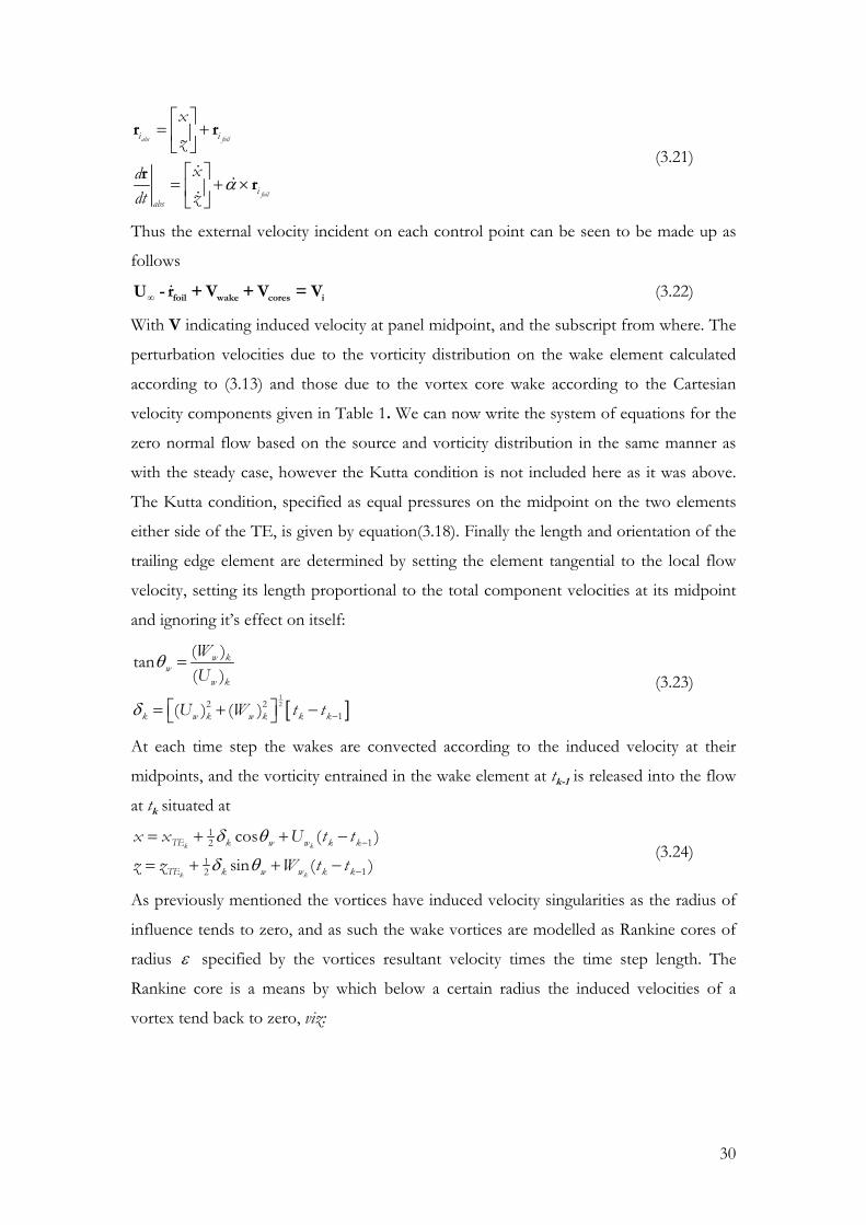
30

abs foil

foil

i i

iabs

xz

xdzdt

α

= +

= + ×

r r

rr

(3.21)

Thus the external velocity incident on each control point can be seen to be made up as

follows

∞ foil wake cores iU - r + V + V = V (3.22)

With V indicating induced velocity at panel midpoint, and the subscript from where. The

perturbation velocities due to the vorticity distribution on the wake element calculated

according to (3.13) and those due to the vortex core wake according to the Cartesian

velocity components given in Table 1. We can now write the system of equations for the

zero normal flow based on the source and vorticity distribution in the same manner as

with the steady case, however the Kutta condition is not included here as it was above.

The Kutta condition, specified as equal pressures on the midpoint on the two elements

either side of the TE, is given by equation(3.18). Finally the length and orientation of the

trailing edge element are determined by setting the element tangential to the local flow

velocity, setting its length proportional to the total component velocities at its midpoint

and ignoring it’s effect on itself:

[ ]122 2

1

( )tan( )

( ) ( )

w kw

w k

k w k w k k k

WU

U W t t

θ

δ −

=

= + −

(3.23)

At each time step the wakes are convected according to the induced velocity at their

midpoints, and the vorticity entrained in the wake element at tk-1 is released into the flow

at tk situated at 1

12

112

cos ( )

sin ( )k k

k k

TE k w w k k

TE k w w k k

x x U t t

z z W t t

δ θ

δ θ−

−

= + + −

= + + − (3.24)

As previously mentioned the vortices have induced velocity singularities as the radius of

influence tends to zero, and as such the wake vortices are modelled as Rankine cores of

radius ε specified by the vortices resultant velocity times the time step length. The

Rankine core is a means by which below a certain radius the induced velocities of a

vortex tend back to zero, viz:

31

Vθ

ε r

Figure 14 Rankine core schematic: below radiusε the induced velocity

decreases linearly to zero, above it follows the relation in Table 1

The system of equations is non-linear and requires an iterative approach for solution.

However, since the model is implemented in Matlab, the inbuilt Gauss-Newton-

Seidel/LU decomposition solver is used to solve the system of equations specifying zero-

tangential flow, and the Kutta condition is implemented as a cost function to be

minimised during solution. At each time-step the values for the length and orientation of

the trailing wake panel are initially estimated, then the system of equations are solved and

the velocity at the midpoint of the wake panel is used to re-specify it’s length and

orientation. The iteration proceeds until convergence which in this model is taken as no

change at double machine accuracy (for both the wake element and the solution of the

governing equations). The results calculated at step k are used to convect the wake and

the foil geometry is re-positioned so that the next time-step calculation may proceed. The

algorithm is summarised in the following chart:

• The foil geometry is defined and the panel influence matrices are set up and hence

begins the time marching section:

1. The foil is positioned according to the simulation time and equations governing

it’s motion, initial estimates for kδ and wθ

a. The perturbation velocities at the midpoints of the panels are calculated

based on the motion of the foil, and the influence of the wake element at

the estimated position, the freestream velocity and the influence of any

shed vortex cores

b. The system of equations is set up, and solved while minimising the Kutta

condition equation

c. The wake panel length and orientation are recalculated based on the

solution at step b based on equation (3.23)

32

2. Part 1 is repeated until the solution converges to the desired accuracy, with no

change in wθ or kδ

3. Wake vortex cores are moved using a Euler approximation based on the

instantaneous velocity measured at their core, made up of the influence of the

foil, the other vortices and the freestream

4. The timestep is advanced and the proto-vortex panel is converted into a vortex

core of strength given by (3.19) and placed according to equation (3.24)

5. Calculation of velocity field, foil surface pressures etc for determining forces and

moments on foil

6. Return to step 1 and continue

The pressure distribution around the foil can be calculated using the unsteady Bernoulli

equation, and this requires that the time rate of change of the velocity potential φ be

known at the midpoint of each panel. This requires that the velocity field must be

integrated from infinitely upstream of the foil to the leading edge, then around the foil to

the panel. A suitable distance for “infinity” is 500 chord lengths, but even with this

approximation, the solution is hugely expensive. Since, to all intents and purposes, only

the hydrodynamic forces on the foil are required in this method the following

simplification is utilised. Because the forces are due to the pressure difference on the

upper and lower surfaces, we can re-cast the Bernoulli equation in terms of the pressure

difference between upper and lower surface panels using the velocity potential and the

velocity at the midpoint of corresponding panels on the upper and lower side:

( ) ( )2 2ˆ ˆ2 2l u

upper lowerupper lower

p p pt tφ φρ

⋅ ⋅ ∂ ∂ ∆ = − = − + −∂ ∂

V τ V τ (3.25)

Thus to calculate the pressure difference we don’t actually require the pressures

themselves we thus only require the difference between the derivative tφ∂

∂ on

corresponding panels – achieved simply by integrating the velocity potential over each

panel at each time-step from the leading edge to the panel midpoint in question.

With the pressure difference per unit length of the foil chord calculated the fluid dynamic

lift and moment about the leading edge may be calculated by

33

2

2

1

01

cos( )

cos( )

N

N

z i i ii

i i i ii

L F p s

M p s x

δ θ α

δ θ α

=

=

≡ = ∆ −

= − ∆ −

∑

∑ (3.26)

Where &is xδ are respectively the length of the i th panel and the distance aft of the LE

of the i th control point. The drag on a 2D foil is during unsteady motion is due to a

combination of induced downwash from the wake and the added mass effect of the

relative fluid acceleration, which correspond respectively to the first and second terms:

1 1

sin( )j

jN

W j k k k kj k

D w st

ρ φ δ θ α= =

∂= Γ + − ∂

∑ ∑ (3.27)

With the sum from k to j being the integration of the velocity potential carried out from

the leading edge then round either the top or bottom surface to wherever the control

point of interest is.

34

Ch. 4 Method Verification and Preliminary Results

In this section, the unsteady panel code is used to model some known flow situations so

that its validity may be ascertained. The results from the code are compared with various

experimental, analytical and numerical results.

The code is then used to model a foil sinusoidally oscillating in pitch and plunge and a

sensitivity study is done in order to determine for future analysis which parameters are

most likely to bear fruit.

4.1 Verification

A number of methods have been used to validate the code during the stages of

development - steady and unsteady results are compared with known results in order to

assure that the code performs as anticipated. Since results from the steady state model

are equivalent to 2D results from an aerofoil in steady flow, the results may be compared

with those from a wind tunnel using a real foil. Pressure tappings on the real foil allow

it’s pressure distribution to be known and measurements typically from potentiometers

and strain gauges, or some kind of balance allow direct and indirect force measurement.

The following graphs show the results from the steady model for the commonly used as

a starting point NACA 0012 foil and the corresponding results from a wind tunnel test.

4.1.1 Steady Code Verification

In order to check that the code is performing at all correctly, the results from the steady

version are used here to determine the aerodynamic coefficients, which are plotted

against known results from Klimas (1981). The results show that the foil is predicting the

shape of the lift curve well, but seems to be slightly over-predicting the actual values. The

panel code does not include viscous effects and as such predicts neither stall nor the

associated increase in drag, but these conditions were accepted and the codes will be used

accordingly.

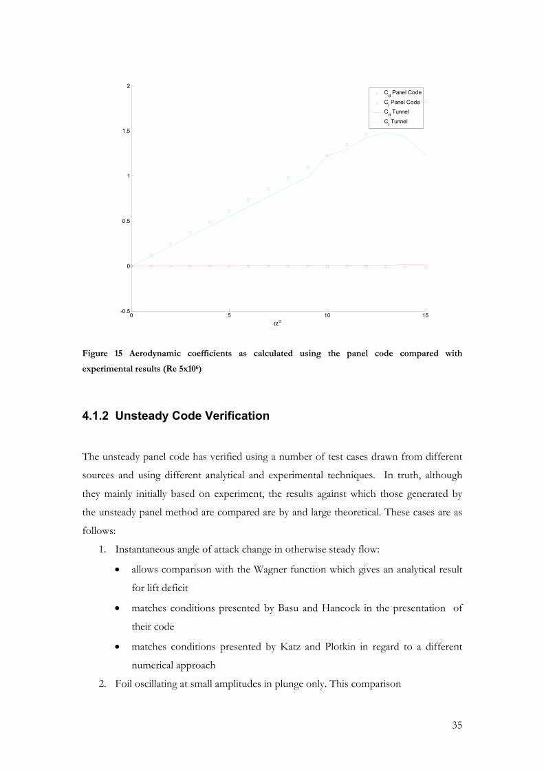
35

0 5 10 15-0.5

0

0.5

1

1.5

2

α°

Cd Panel Code

Cl Panel Code

Cd Tunnel

Cl Tunnel

Figure 15 Aerodynamic coefficients as calculated using the panel code compared with

experimental results (Re 5x106)

4.1.2 Unsteady Code Verification

The unsteady panel code has verified using a number of test cases drawn from different

sources and using different analytical and experimental techniques. In truth, although

they mainly initially based on experiment, the results against which those generated by

the unsteady panel method are compared are by and large theoretical. These cases are as

follows:

1. Instantaneous angle of attack change in otherwise steady flow:

• allows comparison with the Wagner function which gives an analytical result

for lift deficit

• matches conditions presented by Basu and Hancock in the presentation of

their code

• matches conditions presented by Katz and Plotkin in regard to a different

numerical approach

2. Foil oscillating at small amplitudes in plunge only. This comparison

36

• matches conditions analysed by Theodorsen with regard to theoretical

description of phase lag and lift deficit functions

• matches conditions presented by Katz and Weihls (1978) with results for

force coefficients

3. Foil oscillating in both pitch and plunge

• matches conditions analysed experimentally and numerically by Jones et al on

several occasions (notably 1996, 1997).

4. Qualitative comparison of wake formation

• Assess whether the wake evolution matches known results

4.1.3 Instantaneous Angle of Attack Change in Otherwise Steady Flow

The first of these, the step change in incidence, is possibly the most characteristic

situation and serves to demonstrate the unsteady nature of the flow situation. The

Wagner function is a measure of the lag due to wake downwash, and is given as a relation

between transient and steady-state lift values and is often used as a calibration for

unsteady models. A suggested Wagner function for this case is given by Katz & Plotkin

as

( )

( ) 0.091 0.6

1

0.165e 0.335ess W

W

L Lτ τ

φ

φ τ − −

= +

= − − (4.1)

The simulation is set to correspond to the conditions used by Basu and Hancock, namely

a thin symmetrical (von Mises) aerofoil instantaneously pitching to an incidence of .1

radians. The wake roll-up visualisation and the lift time history are presented below, with

the Wagner function and results of Basu and Hancock superimposed. The spike in the

UPC results is due to the integration of the unsteady pressure through the step input and

initial transients, and is the impulsive lift. Basu and Hancock made no attempt to

determine these transients.

The bound circulation on the foil Γ can be easily determined by integrating the wake

circulation and noting that the total circulation in the control volume is required to be

identically zero by conservation. This is presented, along with additional results from a

37

similar case using results from Katz and Plotkin, who used a method whereby the foil is

represented by a number of lumped vortices.

Figure 16 Wake visualisation behind a foil after step change in pitch

0 0.5 1 1.5 2 2.5 3 3.5 4 4.5 50

0.02

0.04

0.06

0.08

0.1

0.12

0.14

0.16Wake circulation distribution behind a foil after a step change in incidence

τ0 0.1 0.2 0.3 0.4 0.5 0.6 0.7 0.8 0.9 10

0.1

0.2

0.3

0.4

0.5

0.6

0.7

0.8

0.9

1

τ

c

Variation in location of the centre of pressure after a step change in incidence

0 0.5 1 1.5 2 2.5 3 3.5 4 4.5 50

0.5

1

1.5

τ

Variation of lift and circulation after a step change in incidence

Γ(t)/ΓssL(t)/Lss UPC

L(t)/Lss UPC

L(t)/Lss Wagner

0 1 2 3 4 5 6 7 8 90

0.005

0.01

0.015

0.02

0.025

τ

Cd

Variation of drag after a step change in incidence

Variation in wake circulation after a step change in incidence

Figure 17 Time variance in lift, drag, CoP and wake vorticity after a step change in incidence as

predicted by UPC

Figure 18 Time variance in wake circulation from Katz & Plotkin

38

Figure 19 Time variance in lift and drag, taken from Basu & Hanckock (lift) and Katz & Plotkin

(drag)

As can be seen from the results, the growth in lift and foil circulation closely matches

predicted values, and additionally the centre of pressure migration is interesting. Since the

CoP is where the sum of moments on the foil due to aerodynamic forces is zero, it is

interesting to see how it is effected by the wake vortex shed, although the migration and

position is intuitive, the rapidity with which it tends to the steady state value is

interesting. However, where the foil is experiencing a complex influence from an number

of strong wake cores, it is likely the CoP migration would put it far in excess of the

deviation shown here, with severe results for stability.

4.1.4 Foil Oscillating at Small Amplitudes in Plunge Only

The Theodorsen lift deficiency function is briefly derived in Ch. 2Error! Reference

source not found. and the function values and phase angles are presented here

graphically for a range of reduced frequencies as calculated using equation (2.10). The

function C(k) is the ratio between the quasi-steady and unsteady lift, and the phase angle

is the phase between steady and unsteady lift. Overlaid is the lift deficit calculated using

the ratio of UPC instantaneous unsteady lift to quasi-steady lift and the phase angle

between them. Note here that k is based on the half-chord.

39

0 0.1 0.2 0.3 0.4 0.5 0.6 0.7 0.8 0.9 10.5

0.6

0.7

0.8

0.9

1

k

C(k)

Theodorsen's lift deficiency function vs. results from unsteady panel code

0 0.1 0.2 0.3 0.4 0.5 0.6 0.7 0.8 0.9 10

5

10

15

20

k

phase φ°

Theodorsen's phase lag function vs. results from unsteady panel code

UPC Soluction Theodorsen's Solution Figure 20 Theodorsen’s functions comparison

The Theodorsen solution is technically only valid for flat plates with infinitesimal plunge

amplitude and a planar wake, when calculating here the wake was allowed to deform as

per the UPC, and the flat plate was approximated by using a farcically thin aerofoil. The

amplitude of the motion was restricted to 120 of the foil chord. The Bessel function

solution for the phase lag has been scaled up by a factor of 2 in accordance with the

results presented in Katz and Plotkin which follow those presented by Wayne Johnston

in Helicopter Theory. The precise value, however, is not relevant and indeed the UPC

result varies slightly with timestep length, number of panels, length of simulation etc – it

is the general trends which are important, and as can be seen they correspond well. The

differences seen at high reduced frequencies are attributable to the evolution of a wake,

since even though the foil motion was infinitesimal, the wake diameter immediately

behind the foil is liable to grow quickly and invaginate, with concentrations of vorticity

forming close to the foil not being convected sufficiently fast that their influence is felt

by the foil on subsequent strokes.

Katz and Plotkin present results from a paper by Katz and Weihls (1978) in which the

vortex wake behaviour behind an oscillating plate is examined. In the paper the forces on

a foil undergoing an oscillatory plunge motion are presented. The difference from the

Theodorsen analysis is that the results are experimental, and also the motion of the foil is

40

finite and the wake fully evolves. The results are used here in comparison with the UPC

results in order to establish whether the periodic forcing characteristics are not only valid,

but also to check that they are accurate in value.

The model is set up in accordance with the conditions presented, namely heaving motion

only, with the following characteristics, and the results are compared. The Strouhal

number is 0.326.

Figure 21 Variation in vertical displacement and normal force during a heaving cycle &

comparison with results from Katz & Weihs (1978)

As can be seen, the model is accurately predicting the magnitude and phase of the

normal force coefficient indicating that the model operates correctly in the finite

magnitude, plunging motion only scenario.

41

4.1.5 Foil Oscillating in Pitch & Plunge

The model is now set up so that the foil travels in plunging motion whilst simultaneously

pitching about an elastic axis. The equations governing the motion are as follows:

( )( )

0 sin

sin

z h tt

ω

α α ω φ

=

= ∆ + (4.2)

Previous works by Jones et al (1997, 2002) have successfully used an unsteady panel code

to investigate numerous parameters effecting the performance and efficiently of both

flapping wing propulsors, and flapping wing power generators. In order to characterise

the performance of the device it is useful to define its efficiency in terms of the ratio of

thrust/drag coefficient to the power coefficient. What this indicates is whether the foil is

providing useful work if the efficiency is less than one, or if the foil is operating well as a

windmill if the efficiency approaches 1 from above. The following results are for a foil

pitching about the quarter chord with a plunge amplitude of .1 chord lengths, with a

phase angle of 90o for a range of angle of attack amplitudes and reduced frequencies. We

would expect to see a discontinuity in the efficiency at the point where the foil switches

from a thrust producing device, to a drag (and hence power) producing device, and we

would expect this discontinuity to lie at the point where the foil is feathered, ie at the

point where the arctan of the Strouhal number is equal to the pitch amplitude.

The discontinuity seems to fit reasonably well for lower frequencies, for example at k = 1

the Strouhal number would be 0.2 and the point of feathering would be with a pitch

amplitude of 11.3α∆ = ° , in Figure 22 it lies across 10 12α∆ = ° − ° . The efficiency as a

windmill approaches 1 from above, and it can be seen that as frequency increases, the

efficiency at taking power from the flow decreases.

The shape and values predicted here are similar to those predicted by Jones et al,

although in Jones case the predicted values for the discontinuities are somewhat higher.

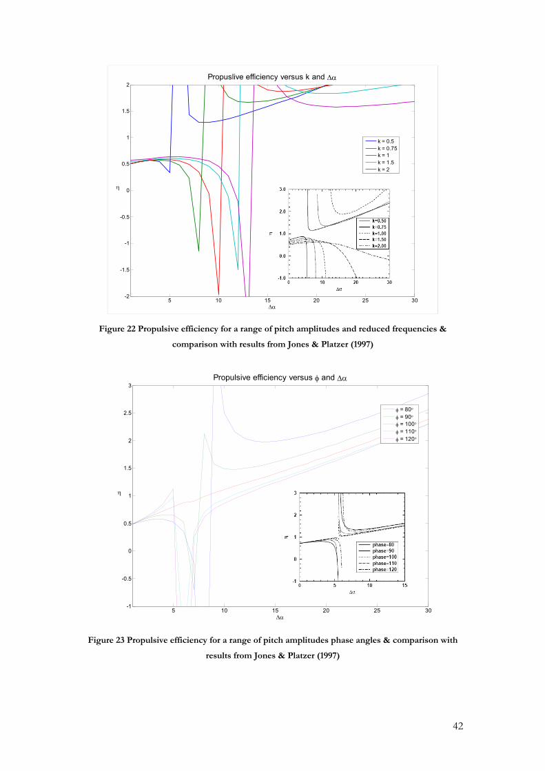
42

5 10 15 20 25 30-2

-1.5

-1

-0.5

0

0.5

1

1.5

2Propuslive efficiency versus k and ∆α

∆α

η

k = 0.5k = 0.75k = 1k = 1.5k = 2

Figure 22 Propulsive efficiency for a range of pitch amplitudes and reduced frequencies &

comparison with results from Jones & Platzer (1997)

5 10 15 20 25 30-1

-0.5

0

0.5

1

1.5

2

2.5

3

∆α

η

Propulsive efficiency versus φ and ∆α

φ = 80°φ = 90°φ = 100°φ = 110°φ = 120°

Figure 23 Propulsive efficiency for a range of pitch amplitudes phase angles & comparison with

results from Jones & Platzer (1997)

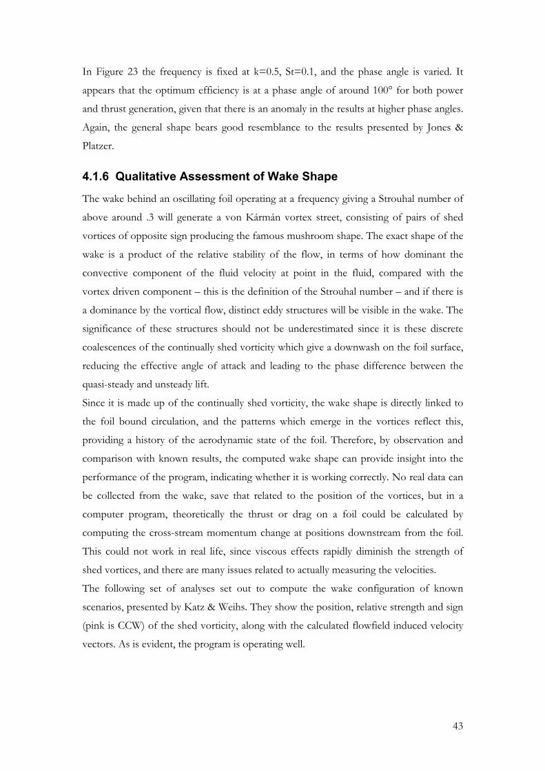
43

In Figure 23 the frequency is fixed at k=0.5, St=0.1, and the phase angle is varied. It

appears that the optimum efficiency is at a phase angle of around 100° for both power

and thrust generation, given that there is an anomaly in the results at higher phase angles.

Again, the general shape bears good resemblance to the results presented by Jones &

Platzer.

4.1.6 Qualitative Assessment of Wake Shape

The wake behind an oscillating foil operating at a frequency giving a Strouhal number of

above around .3 will generate a von Kármán vortex street, consisting of pairs of shed

vortices of opposite sign producing the famous mushroom shape. The exact shape of the

wake is a product of the relative stability of the flow, in terms of how dominant the

convective component of the fluid velocity at point in the fluid, compared with the

vortex driven component – this is the definition of the Strouhal number – and if there is

a dominance by the vortical flow, distinct eddy structures will be visible in the wake. The

significance of these structures should not be underestimated since it is these discrete

coalescences of the continually shed vorticity which give a downwash on the foil surface,

reducing the effective angle of attack and leading to the phase difference between the

quasi-steady and unsteady lift.

Since it is made up of the continually shed vorticity, the wake shape is directly linked to

the foil bound circulation, and the patterns which emerge in the vortices reflect this,

providing a history of the aerodynamic state of the foil. Therefore, by observation and

comparison with known results, the computed wake shape can provide insight into the

performance of the program, indicating whether it is working correctly. No real data can

be collected from the wake, save that related to the position of the vortices, but in a

computer program, theoretically the thrust or drag on a foil could be calculated by

computing the cross-stream momentum change at positions downstream from the foil.

This could not work in real life, since viscous effects rapidly diminish the strength of

shed vortices, and there are many issues related to actually measuring the velocities.

The following set of analyses set out to compute the wake configuration of known

scenarios, presented by Katz & Weihs. They show the position, relative strength and sign

(pink is CCW) of the shed vorticity, along with the calculated flowfield induced velocity

vectors. As is evident, the program is operating well.

44

Figure 24 Comparison with results from Katz & Weihs (1978); 02 8.5 0.009 0.019U tc

U c h cω ∞

∞

∆= = =

Figure 25 Comparison with results from Katz & Weihs (1978); 02 2.1 0.00225 0.019U tcU c h cω ∞

∞

∆= = =

Figure 26 Comparison with results from Katz & Weihs (1978);

02 0.6 0.00065 0.019U tcU c h cω ∞

∞

∆= = =

45

4.2 Sensitivity Analysis

The time stepping UPC is performing as correctly and is now set up in order to do a

sensitivity analysis of the major parameters. The device is set in a nominal configuration

which parallels the operation of the Stingray device and deviations of ± 10 percent are

performed on each parameter and the change in cycle mean power is computed. In an

ideal world it would make sense to vary each parameter by a small amount, say 1%,

however initial results show that not only does this generally produce no significant

change in power output, but it is also unrealistic and of no real value to vary certain

characteristics by such an arbitrary measure. For example: a difference in 1% thickness of

foil one would expect to see no real change in performance, as the lift and drag

characteristics are fairly close for NACA00xx foils and indeed, NACA foils generally are

specified at certain thicknesses where the difference in performance is noticeable, or a

change in phase of 1% is simply insufficient to produce significant and measurable

results at the accuracy the model is being run at.

The Stingray device operated a foil mounted on an approximately 11m arm with a sweep

angle of ± 35° giving an effective stroke amplitude of 6.3 metres. The foil chord (3m) is

used to scale this, resulting in stroke amplitude of 2.1 chord lengths. The Stingray device

was set up to operate at a fixed equivalent incidence through the stroke, but in this model

this is ignored, and the foil incidence follows a sinusoid whose phase angle is 90° lagging

the stroke, resulting in a maximum geometric incidence at the mid-stroke position. The

nominal case parameter values and the altered values are summarised in the following

table: Table 2

Foil Thickness [c] φ° α∆ ° 0h [c] 1secU c −∞

α index

+ 0.165 99 13.5 2.31 1.1 1.1 nominal 0.15 90 15 2.1 1 1

- 0.135 81 16.5 1.89 0.9 0.9 Of these, only the α index requires any further explanation, although the frequencies are

notable by their absence, and both foil pitch and plunge frequencies are set with a period

of 8 seconds. The reason they are not included is that any change in only one would

result in different performance over each stroke as the gulf between the positions on the

cycle of pitch an plunge grew over time – an entirely unreasonable situation. The

frequency for both is altered in a later analysis.

The index of the pitching term is used in the following manner:

( ) sin( it tα α ω φ= ±∆ +

46

with the negative value being used on the “down” stroke, and serves to change to

severity of the pitch rate of change:

0 50 100 150-15

-10

-5

0

5

10

15

t

α

Variation in α(t) with indice

i = 1i > 1i < 1

Figure 27 Variation of incidence with pitch index

The effect is to either increase or decrease the amount of the stroke spent by the foil

close to the maximum incidence, with a reduction in for indices higher than one.

The power coefficient is calculated based on swept area, given by 02h and the assumption

that the foil is one chord length deep.

-10

-5

0

5

10

15

% change in Cp with a 10% change in parameter valuenominal Cp is 0.339 based on swept area

Nominal Thickness φ ∆α h0 U∞ α index

+ - + -

+ -

+ - + -+ -

Figure 28 Sensitivity study results for oscillating foil

47

As is expected, the fundamental parameters are α∆ andφ . The deviation for freestream

velocity is low but bear in mind that the power output from the device is the CP

multiplied by the cube of the velocity, so actually this serves to illustrate that the velocity

has additional effects rather than the normal, cubic relation. This is likely a result of the

fact that the change in freestream velocity acts as a change in effective incidence over the

stroke, due to the Strouhal number relation, and that the downwash due to shed vorticity

is diminished as the vortices are convected away quicker.

As was found by Jones et al the foil thickness has a negligible effect on its performance,

and it is interesting that the stroke length does not significantly affect the power output

at these small deviations. An explanation is that although the foil travels further and

faster, power bonuses from this are swiftly negated by the increased moment required to

turn the foil at the end of the stroke.

The incidence power index yields an interesting result, making it clear that a fuller

incidence profile, such as the 1i < line in Figure 27 is definitely an advantage. This

corresponds with the Stingray project where it was taken to its logical conclusion, and the

foil incidence was set at the maximum for the entire stroke, resulting in a square

incidence profile which yields higher power output. This is to be expected, since the foil

is at its minimum effective incidence at the half stroke position, it makes sense for it to

retain the incidence required here for the complete cycle. Whether this still applies when

viscous effects are brought in remains to be seen, since the foil, while operating at an

optimum incidence at the half stroke, would be operating at a fairly high effective

incidence during the remainder of the stroke, and especially approaching the extremes of

the foil travel – a condition where drag increases rapidly as stall is approached.

The effect of operating frequency is investigated, with the model setup to collect the

power coefficient averaged over 3 cycles for a range of reduced frequencies and pitch

settings. In this instance the power coefficient is based on the streamtube area which is

assumed to be unity (as us foil chord), and as such the relation is simple

P l mC C h C α= +

And the power output can be gotten by multiplying by 312 U Aρ ∞ .

48

1 1.5 2 2.5 3 3.5 4 4.5 5

0

5

10

15

20

25

30-0.3

-0.2

-0.1

0

0.1

0.2

0.3

0.4

0.5

0.6

k

Variation of CP with ∆α and k

∆α

CP

Figure 29 Variation of CP with ∆α and k

Again, if CP is above zero the foil is generating. The frequency and Strouhal number

dependence (the feathering effect) is plainly shown in this diagram: clearly as frequency

rises and power output increases if the foil incidence amplitude is above the crucial value.

49

Ch. 5 Application to the Exemplar Device

In this section the exemplar oscillating foil device will be introduced and the principles of

operation described. The equations of motion will be derived and a solution scheme

involving the unsteady panel code presented. The dynamic free response of the system

under various constraining conditions will be analysed and a fully constrained system

representing the device will developed.

5.1 Description of the Device

The exemplar device is an oscillating foil device requiring no complex control systems,

and is robust and requires very simple moorings – eg it should take very little effort to get

into place, and once in operation it should run without maintenance throughout its

productive lifetime. As intonated during the literature review, one of the main problems

associated with the development and deployment of Stingray was the spiralling

complexity of the device. For this system a certain drop in efficiency, if offset by a simple

design with ease of build and deployment, is acceptable given that a large number may be

deployed at fairly low cost (excluding, of course, the costs of grid connection, underwater

substations etc). Additionally it is intended that the device be fully compatible with

existing marine production techniques and tooling – it is not intended to be an aerospace

specification device – possible advantages in working with these relatively lower

tolerances include lower cost of components and the ability to use existing marine

fabrication plant.

The geometry of the device is shown in the schematic below. It is intended that the foil

angle of attack is fixed (restrained) relative to the mechanical mounting structure of the

device. At the end of the power stroke, power is supplied to change the direction of the

foil motion. The following diagram shows the kinematics of the device and introduces

the nomenclature used hereafter:

50

, θθ

β, β

maxθ R x

z

Figure 30 Schematic of exemplar device

5.2 Equations of Motion

The equations of motion for the device can be derived fully and easily using the Lagrange

energy equation (the large number of parameters, and the degree of coupling make using

Newtonian approaches a daunting prospect). Basically these involve the selection of a

number of generalised coordinates whose values completely describe the position and

states of the system components. The energy equations should yield the same equations

of motion as a small perturbation force analysis using Newton’s second law, and are in

general better suited to use with multiple degree of freedom systems as the method is less

algebraically bulky.

The choice of generalised coordinates must be such that there is no redundancy – they

should be the minimum required to completely describe the state of the system and as

such, in the case of this device, it can be seen from the diagram that they are α and θ .

Thus any conceivable system state can be determined from consideration of these two

ordinates and their derivatives. In quantifying the exemplar system as a kinematic model,

the following assumptions as to the geometry are used:

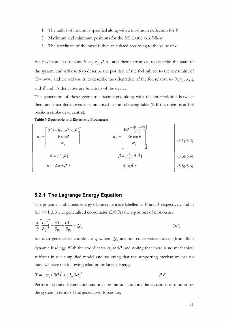
51

1. The radius of motion is specified along with a maximum deflection for θ

2. Maximum and minimum positions for the foil elastic axis follow

3. The z-ordinate of the pivot is then calculated according to the value of e

We have the co-ordinates θ β α, , , ,f f rx z and their derivatives to describe the state of

the system, and will use θ to describe the position of the foil subject to the constraint of

=R const , and we will use αr to describe the orientation of the foil relative to 0xyz . xf, zf

and β and it’s derivative are functions of the device.

The generation of these geometric parameters, along with the inter-relation between

them and their derivatives is summarised in the following table (NB the origin is at foil

position stroke dead centre): Table 3 Geometric and Kinematic Parameters

( )1 sin tansinf

g

R RR

θ θθ

α

− =

x

( )2

2

sin 1 cos

cos

cosf

g

R

R

θ θ

θθ

θ θα

+ =

x

(5.1)(5.2)

( )β θ= ,f r ( )β θ θ= , ,f r (5.3)(5.4)

gα α β= ∆ + ∗ gα β= ∗ (5.5)(5.6)

5.2.1 The Lagrange Energy Equation

The potential and kinetic energy of the system are labelled as V and T respectively and in

for = …1, 2, 3 ,i n generalised coordinates (DOFs) the equations of motion are

∂ ∂ ∂− + = ∂ ∂ ∂

inci i i

d T T V Qdt q q q

(5.7)

for each generalised coordinate iq where incQ are non-conservative forces (from fluid

dynamic loading). With the coordinates αr andθ and noting that there is no mechanical

stiffness in our simplified model and assuming that the supporting mechanism has no

mass we have the following relation for kinetic energy:

( ) αθ α= +2 21 1

2 2f gT m R I R (5.8)

Performing the differentiation and making the substitutions the equations of motion for

the system in terms of the generalised forces are:

52

21

2

00f

g

Qm RQIα

θα

=

(5.9)

The generalised forces can be written in terms of the quasi-steady approximation

(equation (1.2)) as follows:

( ) ( ){ }( ){ }

( )

0 0

0

11 2

12 2 4

1 cossin

cos sin

tan

l l e r d d e r

cl l e EA m e

Re g U R

Q R U S C C C C

Q U Sc C C x C

α α

α α

θ θθ θ

ρ α α θ α α θ

ρ α α

α α∞

∞

∞

−− −

= ⋅ + + − + +

= + − +

= −

(5.10)(5.11)(5.12)

However, as mentioned the quasi-steady approximation does not include any reference

to wake induced velocities on the foil surface, and its use may potentially result in a

model whose accuracy is severely impaired. It is used only as a first approximation, and

the equations are instead integrated using the time-stepping unsteady panel code to

generate the instantaneous hydrodynamic forces on the foil. That said, useful

characteristic information may be obtained by examination of the equations, especially in

relation to angle of attack settings.

The simplified equations given by equation (5.9) are integrated numerically at each time-

step using a 4th order Runge-Kutta (RK4) integrator initially and the Adams-Bashforth-

Moulton predictor-corrector method as follows. However, both methods are only

suitable for integrating 1st order differential equations, so the 2nd order system of

equations of motion are rewritten as four 1st order equations.

5.3 Numerical Integration of the Equations of Motion

We have the equations relating instantaneous forces on the blade given the position and

velocity of the blade at the timestep. In order to calculate the motion of the blade these

must be integrated – essentially integrating the acceleration will give the velocity and

integrating again will give the position. However, care must be taken since it is a double

integration to get the position because any error is likely to propagate rapidly. With this

in mind it is apparent that a simple Euler approximation is insufficient.

The Euler approximation is simply the linear addition of the derivative multiplied by the

timestep length to the previous solution, effectively computing the integral in a single

sum. The RK4 method makes a pair of trial steps in the middle of the time-step and

takes a weighted average of these when returning the final solution, more accurately

53

returning the solution over the step. The system of equations, written in terms of the

generalised coordinates θ and αr is as follows:

( )

( )( )( )

( )

20 0 0

1 0 0 02 2

2 0 1 02 2

3 0 2 0

1 0 1 2 36 1

,

,

,

,

2

EA

f

TT FMk g g gI I m Rk k

t t

t t

Tt

k r r k

X X f X t

X f X X t

X f X X t

X f X tX t t

X X X X X

τ

α αα α θ θ α θ

α α θ θ

+

∆ ∆

∆ ∆

∆+

+

= = =

= + +

= + +

= + ∆ + ∆

= + + + =

(5.13)

The terms subscript 0 and 4 are the time derivatives ( )X at the start and end point of

the thk step; the terms subscript 2 and 3 are the midpoint states and slopes and are

weighted heavier in the calculation of the end states. The function ( ),f X t is the

evaluation of the unsteady panel code run at the four points over the step, and the output

is a vector of the forces and moments, thus accelerations, and the velocities at each point

over the step, equivalent to the derivative (slope) of the system states. The problem here

is that at a high value of t there will be a large number of discrete vortices convecting in

the wake, and as such a function call four times per step becomes extremely

computationally expensive compared with the approach whereby the motion of the foil

is pre-specified (which of course would tell us nothing about the operation of the

exemplar system in which all foil motion is due to fluid forces) – running the simulation

for sufficient timesteps to complete 3 machine power cycles would take over half an

hour at moderate (error tolerance 1e-6) accuracy.

In order to combat this, a predictor-corrector method was used. It is based generally on

using the polynomial expansion of the function derivative ( ),f X t at the start of the step

to predict the function value at the end of the step. This is then used to generate the

function derivative over the step and this in turn is used with the initial conditions to

correct the predicted solution. The method used is the Adams-Bashforth-Moulton

(ABM) method and is based on the Lagrange polynomial expansion of the derivative

based on the current and preceding 3 values, integrated over the step. This yields the

Adams-Bashforth predictor:

( )∆+ − − −= + − + − +1 3 2 124 9 37 59 55P t

k k k k k kX X X X X X (5.14)

54

The corrector is developed from the polynomial expansion about the predicted value

using the current and preceding 2 values, as well as the predicted value just calculated.

This is then integrated giving the solution and is the Adams-Moulton corrector:

( )∆+ − − += + − + +1 2 1 124 5 19 9C t

k k k k k kX X X X X X (5.15)

The derivates X are calculated in the same manner as with the RK4 method, using the

unsteady panel code, but the ABM method only requires 2 calls to the UPC. The error is

the same magnitude as the RK4 method – accomplished by effectively cancelling out the

high order error terms during the derivation – but can be reduced by careful selection of

timestep. The algorithm requires the derivative values from the previous three timesteps,

and these are stored in memory – the code only calls the UPC for the current calculation

and the calculation based on the predictor. This significantly reduces the computational

time, fewer function calls coupled with a slightly increased timestep length result in a

computation time of around 10 minutes for the same 3 cycle simulation and tolerance as

mentioned previously. However the ABM method is not self starting: it requires the

previous three function derivatives which are not available during the initiation of the

simulation. These are providing by using the RK4 method for the first few timesteps

then switching over after the fourth step.

55

Ch. 6 Modelling of the Exemplar & Some Results

In this section the equations of motion for the oscillating foil device described previously

are used alongside the unsteady panel code to model the device. The code is setup in

such as way that the operation of the device is cyclical, ie the foil is put over at the end of

each power stroke ready for the next one, and the model is allowed to run for several

cycles. The addition of a damping coefficient to the equations of motion, representing

power take off is evaluated, and power curves determined for various parameters based

on a sensitivity study.

6.1 Setting up the Model

As mentioned in preceeding chapters, the device consists of a foil whose pitch and drag

are reacted by some means. At the extreme of each cycle power is required to turn the

foil to reverse the cycle.

6.1.1 Modelling the Put Over

In order to accommodate the process of putting over the foil into the model it is

necessary to define conditions whereby the foil is either locked into place by the support

mechanism at the extremes of the angle of attack range, or free to rotate according to

Newton’s second law. The reason that the model is set up like this is computational: it is

easier to program and it prevents spikes in forces due to impulse loading messing up the

integration. Ease of programming is an issue since the model is growing increasingly

complex, and error minimisation is essential. Impulsive loading occurs when the foil is to

move, but reaches a mechanical restraint. This leads to numerical “spikes” in the forcing

calculation which can cause excessive velocities when integrated but since the loading is

impulsive, due to the fact that the foil has moved away (at high speed) from the

constraint mechanism, the hydrodynamic forces dominate at the next time step, and the

foil can be returned to the constant. Aside from the massive instantaneous change in

velocity potential and the computed shedding of artificially high wake vorticity, the foil

becomes trapped in a computational loop continuously rebounding from the constraint

mechanism. Eventually the simulation breaks down

due to large numbers overwhelming the integrator and the solver for the UPC or the

computer overflows.

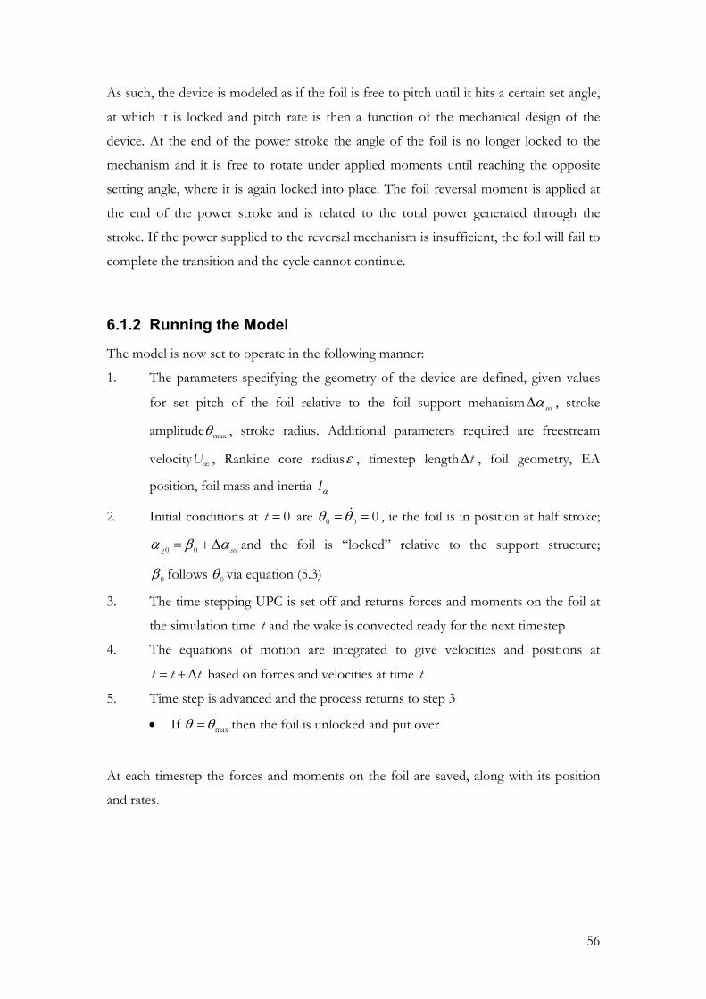
56

As such, the device is modeled as if the foil is free to pitch until it hits a certain set angle,

at which it is locked and pitch rate is then a function of the mechanical design of the

device. At the end of the power stroke the angle of the foil is no longer locked to the

mechanism and it is free to rotate under applied moments until reaching the opposite

setting angle, where it is again locked into place. The foil reversal moment is applied at

the end of the power stroke and is related to the total power generated through the

stroke. If the power supplied to the reversal mechanism is insufficient, the foil will fail to

complete the transition and the cycle cannot continue.

6.1.2 Running the Model

The model is now set to operate in the following manner:

1. The parameters specifying the geometry of the device are defined, given values

for set pitch of the foil relative to the foil support mehanism setα∆ , stroke

amplitude maxθ , stroke radius. Additional parameters required are freestream

velocityU∞ , Rankine core radiusε , timestep length t∆ , foil geometry, EA

position, foil mass and inertia Iα

2. Initial conditions at 0t = are 0 0 0θ θ= = , ie the foil is in position at half stroke;

0 0g setα β α= + ∆ and the foil is “locked” relative to the support structure;

0β follows 0θ via equation (5.3)

3. The time stepping UPC is set off and returns forces and moments on the foil at

the simulation time t and the wake is convected ready for the next timestep

4. The equations of motion are integrated to give velocities and positions at

t t t= + ∆ based on forces and velocities at time t

5. Time step is advanced and the process returns to step 3

• If maxθ θ= then the foil is unlocked and put over

At each timestep the forces and moments on the foil are saved, along with its position

and rates.

57

6.2 Some Results

Since the device is theoretical, the defining parameters may be assigned based on

engineering judgement and prior results. In order to test the device, it is worth setting up

a base case from which parameters may be adjusted for performance. The device

parameters used here follow a rough trial and error approach using Simulink and the

quasi-steady approximation.

The model is set up with the following parameters and allowed to run for 500 timesteps.

Angle of attack, force, moment and position histories are presented for a number of

cycles although due to the computational expense of running the program for particularly

long, the cycles are amongst the first few after the device is initiated, and as such show

some asymmetry.

Table 4 Device Geometric Parameters

U∞ 11 secc − Foil shape NACA0012 α∆ 10° EA position 0.7 c aft of LE

maxθ 0.07 4rads ≈ ° t∆ 0.01

R 20 c Iα 22.5mc m 1

20 40 60 80 100 120 140-15

-10

-5

0

5

10

15Variation of θ, effective and geometric incidence over 2 cycles

Simulation time

as indicated

θ°αg°

αe°

Figure 31 Variation of parameters over cycles (undamped device)

58

The geometric angle of attack history follows predictably from the specification that

gα β α= + ∆ with the incidence locked over a large part of the cycle. As can be seen, the

angle of attack is dependant on β which may reduce eα substantially, and the effective

angle of attack crosses zero close to the end of the stroke.

The full energy balance for the system takes into account the power absorbed by moving

the foil through the stroke and the power required to pitch the foil at the end of the

stroke. The power to flip the foil is needed to overcome the foil inertia in pitch and the

hydrodynamic forces generated. If either of these are too great then the mechanism may

not be able to generate sufficient moment with the available power in the time required

and the foil will end up stuck.

The instantaneous power equation is

P F Rθ τθ= ⋅ (6.1)

which must be time averaged over a cycle to get the power output

( ) ( )0

TRP t F t dtTθ τθ= ⋅∫ (6.2)

The power required to put over the foil may be calculated in a similar manner:

EAP Mα α= ⋅ (6.3)

20 40 60 80 100 120 140-1.2

-1

-0.8

-0.6

-0.4

-0.2

0

0.2

0.4

0.6

Simulation time

as indicated

Power variation, αe and θ across 2 cycles

Power Wθ radsαe rads

Figure 32 Variation of parameters across 2 cycles

59

As is clear, when the foil is being flipped there is work being done by the foil and power

is negative, however since this is effectively “free” power it may be written off, as long as

it is appreciated that to increase device efficiency it would be useful to minimise it and

this will undoubtedly involve a trade off between maximum power over the stroke and

the inherent problems with momentum. Essentially, as long as the area on the power

curve above the time axis across the stroke is greater than or equal to the area below,

then the foil should flip, with any extra power being usable output.

The graph again shows the zero crossing of the effective angle of attack at the tail end of

the stroke, but by observation it appears that the power stroke here is dominated by

inertial motion as opposed to forced movement, and as such lags the effective incidence

somewhat.

The power generated during the stroke is now considered in isolation, with any losses due

to putting over the foil being taken as rote. The model is set so that the effect of varying

parameters may be investigated and their effect on power output determined. The results

of this sensitivity study are inconclusive, as due to the non-linear nature of the system

and the inherent coupling effect of changing parameters, certain modifications to the

system result in an increase or decrease in performance after being altered in both the

plus and minus direction. It is appreciated that this does not necessarily imply a global

maxima or minima at the point of investigation and that further work will reveal more

useful trends.

The chart below shows the percent change in power output of the device, given a

10± % change in the value of the parameter of interest, everything else held the same.

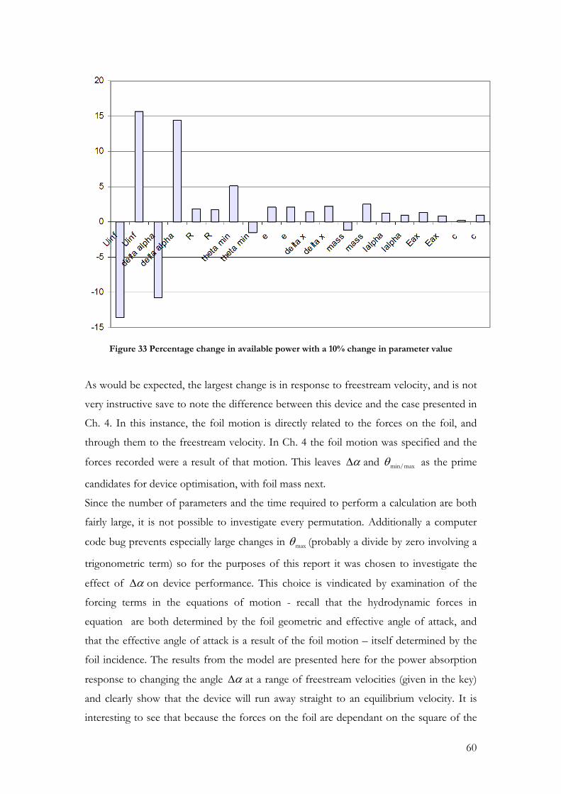
60

Figure 33 Percentage change in available power with a 10% change in parameter value

As would be expected, the largest change is in response to freestream velocity, and is not

very instructive save to note the difference between this device and the case presented in

Ch. 4. In this instance, the foil motion is directly related to the forces on the foil, and

through them to the freestream velocity. In Ch. 4 the foil motion was specified and the

forces recorded were a result of that motion. This leaves α∆ and min/maxθ as the prime

candidates for device optimisation, with foil mass next.

Since the number of parameters and the time required to perform a calculation are both

fairly large, it is not possible to investigate every permutation. Additionally a computer

code bug prevents especially large changes in maxθ (probably a divide by zero involving a

trigonometric term) so for the purposes of this report it was chosen to investigate the

effect of α∆ on device performance. This choice is vindicated by examination of the

forcing terms in the equations of motion - recall that the hydrodynamic forces in

equation are both determined by the foil geometric and effective angle of attack, and

that the effective angle of attack is a result of the foil motion – itself determined by the

foil incidence. The results from the model are presented here for the power absorption

response to changing the angle α∆ at a range of freestream velocities (given in the key)

and clearly show that the device will run away straight to an equilibrium velocity. It is

interesting to see that because the forces on the foil are dependant on the square of the

61

foil velocity the power relation with incidence is not linear, as one would expect - the

effective incidence is also dependant on the square of the foil velocity, and consequently

there is a slight quadratic nature to the power curves.

1secU c −∞

α∆ °

%PC

Figure 34 Power coefficient curves at various incidence settings and velocities

The device was found to be unable to complete the pitch transition at any freestream

velocity for 15α∆ ≈> ° and thus the highest power available at the device is at below 15

degrees set incidence. Again the momentum conservation issue is to blame and the

device lacks the momentum at the top of the stroke to overcome the moment on and the

inertia of the foil.

The power from the device over the stroke is the product of the force and velocity of the

foil, and as such can have 2 minima: the non-trivial one is where the effective incidence

of the foil is zero and there is a force balance. The problem with the device is that it is

not constrained in any meaningful sense and experiences no retarding force except the

component of drag acting in the direction opposite the motion of the foil. As such it

simply accelerates as fast as it can to the point where it either meets the stop at the end of

the cycle, or it reaches equilibrium and 0eα = . The following diagram was made using

the steady state values for the aerodynamic coefficients as shown in Figure 15 in the

quasi-steady approximation for the foil traversing the cycle at various rates. At velocities

higher than that at point (1) the foil will require power input to accelerate.

62

0 0.05 0.1 0.15 0.2 0.25 0.3-0.05

0

0.05

0.1

Vstroke/U∞

Power Captured

Power captured with stroke velocity as fraction of U∞ for ∆α=15°

1

2

Figure 35 Relation between stroke velocity and power

Thus it is evident that as the device fails at set incidences above 15 degrees, it is operating

at or just before point (1) on the curve and it is intuitively correct that if the foil were

having any form of power taken off as it operates close to point (1) that it would

immediately have insufficient momentum to make it over the transition. Conversely it is

also intuitively correct that if the foil was set at a lower pitch and retarded, the effective

incidence could be maintained closer to the optimum without the foil running away, and

if the retarding force was correctly administered if excess mean power was available after

the foil had done the pitch transition it would be available to take off without the foil

getting stuck. The foil would then be able to theoretically operate close to point (2).

6.3 Introducing a Damping Coefficient

In order to achieve the theoretical increase in device performance associated with foil

motion being retarded, a damping coefficient is introduced into the equations of motion.

This effectively applies a force on the foil acting opposite in direction to the motion of

63

the foil, and of magnitude proportional to the velocity of the foil. The constant of

proportionality is literally the damping coefficient and this is it in application in the

simplest sense. The equations of motion of the device equation (5.9) (minus supporting

stucture terms) are now re-written with the damping coefficient is included in the model,

and integrated alongside the other terms. 2

1

2

000

f

r

c Qm RQIα

θ θα α

+ =

(6.4)

It is clear that the total power available to the foil can be split into the part required to

flip the foil and that “lost” to the damping effect. Since the damping term effectively acts

as a brake then this could be considered friction, but if the damping represented a power

take off device, then the work done here would be the useful power and energy output of

the device. Thus the instantaneous power equation of the device is simply 2

dampP cθ= (6.5)

And this represents a certain fraction of the total power taken from the fluid flow by the

device such that we can define the device efficiency as the ratio of power taken to total

power available

312 P

c cF R c U SCτ

θ θηθ ρ ∞

= =⋅ +

(6.6)

The effect of damping the motion is going to alter the power curves presented above: it

is obvious that if at 15α∆ ≈ ° the device is failing without damping, then any power take

off is not going to aid the situation and it is likely that at angles of attack close to 15

degrees the device will fail with a small damping coefficient and the power output would

be less than that at a lower pitch. This is demonstrated in device results showing the

excess power available at various pitch settings with different damping coefficients (note

that the black line is actually through the peaks of the other lines and the humps at the

end are a result of over enthusiasm on the part of Excels curve fitter):

64

Excess Power vs "Damping"

0

0.05

0.1

0.15

0.2

0.25

0.3

0.35

0.4

0 0.2 0.4 0.6 0.8 1 1.2 1.4 1.6 1.8

Damping Coeff icient

Pow er

8deg 9 deg 10 deg11 deg 12 deg 13 deg

14 deg P_max

Figure 36 Excess available power versus damping

There is no result for 15° as the device has failed and the mean power over the cycle

cannot be calculated. The power “lost” to damping is shown in the following chart,

which shows the maximum power output at each incidence alongside the efficiency

7 8 9 10 11 12 13 14 150

0.1

0.2

0.3

0.4

0.5

0.6

0.7

∆α

η & Power

Efficiency and power output

ηPower

Figure 37 Maximum power output and efficiency at a range of angles of attack

It is now clear that the most effective pitch setting is around 11° for this particular device

configuration. Unfortunately the parameter space is extremely large with many more

permutations available than time will allow full investigation of, and it is accepted that

there are likely better power outputs possible.

65

What is interesting, though, is the behaviour of the device close to the point where the

device fails – i.e. where it operates optimally. Comparing these results with the results

from a foil oscillating in pitch and plunge, it appears that the shape and structure of the

power output bears resemblance to data presented Figure 22, and this becomes more

apparent when the results are plotted in terms of power and incidence at the optimum

damping coefficient:

0 2 4 6 8 10 12 14 16 180

0.05

0.1

0.15

0.2

0.25

0.3

0.35

0.4

0.45

∆α

as indicated

Variation of power captured, excess power, power required to flip foil,frequency of operation and equivilent incidence given by αe=tan-1(St)

Pflip WPcapt W

ω rads-1

ωfit rads-1

0.01×α°e

0.01×α°efitPavail W

Figure 38 Variation in power, frequency and equivalent incidence for device working optimally

It can be seen that the incidence setting for optimum operation is very close to that given

by 1tan ( )St− and this indicates that at the optimum damping setting the device behaves

in a manner very similar to a foil operating close to optimum efficiency in sinusoidal

motion. It should also be noted that there appears to be a trend in efficiency as the

frequency (or pitch amplitude) of operation decreases, with the power captured coming

closer and closer to the power required to flip the foil. This corresponds nicely with the

results from the analysis of the sinusoidally oscillating foil in which an increase in

propulsive efficiency followed from a decrease in frequency. However, it should be

remembered that one of the conditions of the model is the inviscid nature of the

calculation, and it is likely that as the pitch amplitude is reduced the foil motion would be

more subject to viscous drag, possibly reducing the power captured and hence the

efficiency.

66

Ch. 7 Summary & Conclusions

This thesis has reported on the development of an unsteady panel code solver which has

been used to investigate parameters important to the power output from an oscillating

foil. This has been done by investigation of a generic foil oscillating in pitch and plunge

with specified amplitude and frequency and then extended via a dynamic model of a

exemplar system based on a simple control mechanism and operating procedures.

The results from the parameter investigation of the generic foil indicate that there is

sensitivity of device performance to pitch and phase angles, as one would expect, and

additionally to the shape of the pitch profile, again as would be expected.

The sensitivity of the oscillating foil power output on frequency has been investigated,

and the dependency on Strouhal number demonstrated, with a definite trend indicating

that the frequency of oscillation where a foil moves from thrust generation to power

capture is reasonably approximated by the arctan of the Strouhal number.

The index of pitch change has shown a positive effect on the power output, with power

output increasing as the index decreased, ie as the pitch history became fuller.

These provide incentive to investigate the performance of a device whose pitch profile is

almost square, and such a device has been included in the investigation. The main

outcomes from the investigation of the exemplar device are initially that it seems to

function as designed, although power output can be fairly low, and that its performance

is dependant on angle of attack setting in the same way as the generic device whose

motion is purely sinusoidal.

The motion of the foil was found to reach an equilibrium if unrestrained, at which point

no power could be delivered – a result of the foil decreasing its effective incidence to

zero. The addition of a damping term has allowed computations of simulated power take

off, the effect of which is to retard the foil motion, and the critical power take off level

has been established as that above which the foil is unable to complete a pitch change.

Based on these considerations, the optimum power output from the device was found to

be at an incidence lower than the maximum allowed, due to the relatively higher forces

on the foil during the power stroke, facilitated by the slower foil speed increasing the

effective incidence, and the lower pitching moment to be overcome at the extreme of the

foil travel.

67

Theoretically with the addition of the damping term the foil should come to an

equilibrium velocity whose value is determined by the damping coefficient and the

hydrodynamic forces, and we can solve for this steady state solution by using the fact

that at the equilibrium the acceleration is zero and by use of the quasi-steady

approximation, ie:

( ) ( ){ }( )

0 0

12

1 cossin

cos sin

tan

l l e r d d e r

Re r U R

c R U S C C C Cα α

θ θθ θ

θ ρ α α θ α α θ

α α∞

∞

−− −

= ⋅ + + − + +

= −

(7.1)(7.2)

it is apparent that the foil equilibrium velocity will vary across the stroke due to the terms

representing β however, so if this equation were used as a guideline for setting device

parameters, an iterative approach would have to be adopted, and the result would

indicate as to whether the foil had reached its equilibrium velocity before the maximum

excursion. This would yield useful information about the power output from the stroke,

and is a means of investigating maximising the full power phase of the stroke.

Unfortunately, there was insufficient time to investigate this further, but it could prove

the basis for further work.

Consideration of the frequency of operation yields the final result, which is that at the

optimum damping coefficient for a foil incidence, that incidence is very close to the

arctan of the Strouhal number of the device operation. This seems to hint that the device

performs, at its highest efficiency, in a comparable manner to a sinusoidally oscillating

foil at the same frequency and pitch given by α∆ . It also allows the inverse result: that

the frequency of operation for the device at the optimum power setting may be

determined from consideration of the Strouhal number at that point. This result should

allow the calculation of device performance using a simple time stepping algorithm like

the one presented in Ch. 3 rather than the full integration of the equations of motion

with all the associated savings in computational cost.

The recommendations for future work rest on the requirement for a more complete

understanding of the fluid mechanics of the unsteady flow situation. The foil model is

able to predict vortex shedding from the trailing edge only, as stipulated by the Kutta

condition, but it is possible for leading edge vortices to have significant effect on the

performance of the system, as alluded to in the literature review, by effectively becoming

entrained within the TE vortices, with an effect much like constructive or destructive

68

interference. The effect of these on the exemplar device, as well as the effect and

prevalence of dynamic stall situations, where peculiarities with oscillatory flow cause

delayed stall and a cyclic nature to the hydrodynamic forcing, should feature as part of

future work.

The work in this thesis is concerned with the shed wake from the foil, and being based

on an inviscid analysis does not realistically predict the dissipation of the eddies. It would

be of particular use to develop an understanding of the breakdown of the wake structure

as it convects downstream, and additionally to add to the model the effects of operation

close to the seabed, namely the presence of a log law velocity profile and a boundary

close to one side of the device. Jones et al (2002) demonstrate an addition to a panel code

whereby the effects of a boundary are included by mirroring the wake and panels over a

line of symmetry, in order to predict the operation of the foil in ground effect. The same

approach could be adopted, along with the log law profile and some semi-empirical

means of calculation of wake dissipation, leading to a greater understanding of the

environmental implications and Significant Impact Factor of the device. This sort of

study would most likely be required as part of any application for funding, and definitely

be required prior to prototype testing.

Additionally, since the parameter space is quite large, with geometric and fluid mechanic

properties having significant and non-linear effects on system performance, a fuller

treatment of the governing equations for the system should be performed in order to

illuminate the parameters most likely to boost performance, and resolve the local minima

phenomenon experienced during the sensitivity study of the device.

A final recommendation is that future work be carried out outside of Matlab. While

useful as a tool, it is a fairly inefficient working environment when doing long high

memory calculations and has a tendency to crash. This was an issue during the work,

since the UPC and the integrator both operate at fairly fine tolerances, and when the

numbers of iterations to find optima are factored in it can take an exceptionally long time

- the computer time required to make Figure 38 was around 60 hours on a fast dual core

PC, collating more than 200 results. Therefore, in addition to pre-selecting criteria to

investigate as mentioned in the preceding paragraph, it would help if the modelling was

done using a low level computer language on dedicated computers such as Sun Solaris.

69

Ch. 8 References & Bibliography

Adamko, D., DeLaurier, JD (1978). "An experimental study of an Oscillating Wing

Windmill." Proceedings of the Second Canadian Workshop on Wind Engineering 64-66.

Ansari, S., R. Bikowski, et al. (2006). "Non-linear unsteady aerodynamic model for insect-

like flapping wings in the hover. Part 1: methodology and analysis." Proceedings of the I

MECH E Part G Journal of Aerospace Engineering 220: 61-83.

Ansari, S., R. bikowski, et al. (2006). "Non-linear unsteady aerodynamic model for insect-

like flapping wings in the hover. Part 2: implementation and validation." Proceedings of

the I MECH E Part G Journal of Aerospace Engineering 220: 169-186.

Basu, B. C. and G. J. Hancock (1978). "The unsteady motion of a two-dimensional

aerofoil in incompressible inviscid flow." Journal of Fluid Mechanics Digital Archive

87(01): 159-178.

BBC. (2006). " Compromise saves climate treaty" Retrieved 03 July 2006, from

http://news.bbc.co.uk/1/hi/sci/tech/1452315.stm.

BBC. (2006). "Warning over tidal energy impact." Retrieved 03 July 2006, from

http://news.bbc.co.uk/1/hi/scotland/3580484.stm.

Cheng, J.-Y. and G. L. Chahine (2001). "Computational hydrodynamics of animal

swimming: boundary element method and three-dimensional vortex wake structure."

Comparative Biochemistry and Physiology - Part A: Molecular & Integrative Physiology

131(1): 51-60.

Couch, S., Bryden, I. G. (2004). "MAREC Paper: The impact of energy extraction on

tidal flow development." Retrieved 03 May 2006.

Dowell, E. H. (1995). A modern course in aeroelasticity Kluwer Academic.

70

DTI. (2002). "RESEARCH AND DEVELOPMENT OF A 150kW TIDAL STREAM

GENERATOR - Phase 1." Retrieved 02 May 2006, 2006, from

http://www.dti.gov.uk/renewables/publications/pdfs/T00211.pdf.

DTI. (2003). "RESEARCH AND DEVELOPMENT OF A 150kw TIDAL STREAM

GENERATOR - Phase 2." Retrieved 02 May 2006, 2006, from

http://www.dti.gov.uk/renewables/publications/pdfs/T00211.pdf.

DTI. (2005). "Stingray Tidal Stream Energy Device – Phase 3." Retrieved 02 May 2006,

2006, from http://www.dti.gov.uk/renewables/publications/pdfs/T00211.pdf.

Fung, Y. C. (1993). An introduction to the theory of aeroelasticity Dover Publications.

Garrick, I. E. (1937). "Propulsion of a flapping and oscillating airfoil." NACA Report

567.

Greenblatt, D. and I. J. Wygnanski (2000). "The control of flow separation by periodic

excitation." Progress in Aerospace Sciences 36(7): 487-545.

Guglielmini, L., P. Blondeaux, et al. (2004). "A simple model of propulsive oscillating

foils." Ocean Engineering 31(7): 883-899.

Hassan, G. (2004). UK Atlas of Offshore Renewable Energy, DTI.

Hedenström, A. (2002). "Aerodynamics, evolution and ecology of avian flight." Trends in

Ecology & Evolution 17(9).

Hess, J. L. and A. M. O. Smith (1967). "Calculation of potential flow about arbitrary

bodies." Progress in Aerospace Sciences 8: 1-138.

Hover, F. S., O. Haugsdal, et al. (2004). "Effect of angle of attack profiles in flapping foil

propulsion." Journal of Fluids and Structures 19(1): 37-47.

71

Jones, K. D., Dohring, C.M., Platzer, M.F. (1996). "Wake structures behind plunging

airfoils: a comparison of numerical and experimental results." AIAA Paper 96-0078.

Jones, K. D., Platzer, M.F. (1997). "Numerical computation of flapping-wing propulsion

and power extraction." AIAA Paper 97-0826.

Jones, K. D., Davids, S., Platzer, M.F (1999). "Oscillating-wing power generation."

Proceedings of the 3rd ASME/JSME Joint Fluids Engineering Conference.

Jones, K. D., Platzer, M.F (2001). "On the use of vortex flows for the propulsion of

micro-air and sea vehicles." NATO R&T Organisation Applied Vehicles Technology

Panel Week.

Jones, K. D., Castro, B,M., Mahmoud, O., Platzer, M.F (2002). "A numerical and

experimetnal investigation of flapping-wing propulsion in ground effect." AIAA Paper

2002-0866.

Katz, J., Weihs, D. (1978). "Behaviour of vortex wakes from oscillating foils." AIAA

Journal of Aircraft 15(12): 861-863.

Katz, J., Plotkin, A. (2001). Low speed aerodynamics. Cambridge, Cambridge University

Press.

Klimas, P. and R. Sheldahl (1981). Aerodynamic Characteristics of Seven Symmetrical

Airfoil Sections Through 180-Degree Angle of Attack For Use In Aerodynamic Analysis

of Vertical Axis Wind Turbines. Albuquerque, Sandia National Laboratories.

Koochesfahani, M. M. (1989). "Vortical patterns in the wake of an oscillating airfoil "

AIAA Journal 27(9): 1200-1205.

Lehmann, F.-O. (2004). "Aerial locomotion in flies and robots: kinematic control and

aerodynamics of oscillating wings." Arthropod Structure & Development 33(3): 331-345.

72

Lighthill, M. J. (1969). "Hydrodynamics of aquatic animal propulsion." Annual Review of

Fluid Mechanics 1: 413-446.

Lighthill, M. J. (1970). "Aquatic animal propulsion of high hydromechanical efficiency."

Journal of Fluid Mechanics 44(2): 265-301.

Liu, H., Kawachi, K. (1999). "A Numerical Study of Undulatory Swimming." Journal of

Computational Physics 155: 223-247.

Liu, P. and N. Bose (1999). "Hydrodynamic characteristics of a lunate shape oscillating

propulsor." Ocean Engineering 26(6): 519-530.

Lu, X., Yang, J., Yin, X. (2003). "Propulsive performance and vortex shedding of a foil in

flapping flight." Acta Mechanica 165: 189-206.

Maskel, E. C. (1972). On the Kutta–Joukowski condition in two-dimensional unsteady

flow, Royal Aircraft Establishment, Farnborough.

McKinney, W. a. D., J., (1981). "The Wingmill: An Oscillating-Wing Windmill " AIAA

Journal of Energy 5(2): 109-115.

Munsen, B., D. Young, et al. (1998). Fundamentals of fluid mechanics. New York, John

Wiliey & Sons.

Platzer, M. F., Jones, K.D. The unsteady aerodynamics of flapping-foil propellers,

Deptarment of Aeronautics and Astronautics, Naval Postrgraduate School, Monterey

Ca., USA.

POST (2004) “The future of UK gas supplies.” Postnote 230, Parliament Office for

Science & Technology

Read, D. A., F. S. Hover, et al. (2003). "Forces on oscillating foils for propulsion and

maneuvering." Journal of Fluids and Structures 17(1): 163-183.

73

Rozhdestvensky, K. V. and V. A. Ryzhov (2003). "Aerohydrodynamics of flapping-wing

propulsors." Progress in Aerospace Sciences 39(8): 585-633.

Schmidt, W. (1965). "Der Wellpropeller, ein neuer Antrieb fuer Wasser-, Land-, und

Luftfahrzeug." Z. Flugwiss 13: 472-479.

Schouveiler, L., F. S. Hover, et al. (2005). "Performance of flapping foil propulsion."

Journal of Fluids and Structures 20(7): 949-959.

Sfakiotakis, M., Lane, D.M., Davies, J.B.C. (1999). "Review of Fish Swimming Modes for

Aquatic Locomotion." IEEE Journal of Ocean Engineering 24(2).

Smith, M. J. C., Wilkin, P.J., Williams,. M.H. (1996). "The advantages of an unsteady

panel method on modelling the aerodynamic forces on rigid flapping wings." Journal of

Experimental Biology 199: 1073-1083.

Streitlien, K. and G. S. Triantafyllou (1998). "ON THRUST ESTIMATES FOR

FLAPPING FOILS." Journal of Fluids and Structures 12(1): 47-55.

Techet, A. H. H., F.S., Triantafyllou, M.S. (2003). "Seperation and Turbulance Control in

Biomimetic Flows." Flow, Turbulance and Combustion 71: 105-118.

Theodorsen, T. (1935). "General theory of aerodyanmic instability and the mechanism of

flutter." NACA TR-496.

Triantafyllou, G. S., M. S. Triantafyllou, et al. (1993). "Optimal Thrust Development in

Oscillating Foils with Application to Fish Propulsion." Journal of Fluids and Structures

7(2): 205-224.

Triantafyllou, M. S., Techet, A.H., Hover, F.S. (2004). "Review of Experimental Work in

Biomimetic Foils." IEEE Journal of Ocean Engineering 29(3).

von Kármán, T., Burgers, J.M. (1943). "General aerodynamic theory: Perfect fluids."

Aerodynamic Theory 2(Division 3).