Performance Evaluation of Computer Systems and

Networks Lecture notes for CS 681

Varsha ApteDepartment of Computer Science and Engineering

IIT Bombay. Spring - 2015.

[Lecture 1: January 5th, 2015]

1 Motivation

We experience the impact of contention for resources almost continuously in our daily lives. Thetraffic on the road, the lines at a supermarket, the crowd on a Sunday evening at a McDonalds -these are all examples of resources under contention.

Computing Systems and networks are no different. There are a variety of different resources inthese systems that could easily come under contention. Can you name a few? In fact, as end-users of such systems we frequently experience the effects of this contention (“slow” website, “slow”network, etc).

Table 1 shows some resources and the “customers” that use these resources.

Resource Users (Schedulable Entity)CPU Processes, ThreadsPrinter Print JobsWeb Server Threads HTTP GET/POST requestsData Network Link PacketsCellular Network Channel Cellular Call

Table 1: Examples of resources and their users. “Users” are the scheduling unit, the entity that ischosen for resource allocation

Now consider one of these resources, let’s say, a Web server, that is to be specific, the threadpool of a Web server process. The thread pool of a Web server is a limited resource. An arrivingHTTP request is given a thread if there is an idle thread, or joins a queue of requests at the end, ifall threads are busy.

What performance-related questions can we ask about the system? What are the variables thatdetermine the performance of the system? When you think of such systems, always classify thequantities into parameters and metrics.

Thus we could ask the question as to “What is the average waiting time of a request”, when thearrival rate is 100 requests/sec? Here, waiting time is an example of a metric.

The answer to this question will depend on various quantities, e.g., it will depend on the averageprocessing time per request, request arrival rate or on the number threads that the Web server isconfigured with. These are examples of parameters.

1

Parameter Unit1 CPU Speed GHz, flops/sec , MIPs2 Request Arrival Rate requests/sec3 Average resource requirements per request Depending on the resource,

e.g. for CPU MI/request4 Disk read write rate blocks/sec5 Buffer Size

Table 2: Parameters

Metric is something by which we judge a system. This is what we observe, measure, evaluate.Parameter is what we change to see how it affects a metric. This difference in metrics and parametersis important to note in system evaluation.

Figure 1: Parameters and Metrics

Think of various such performance metrics and parameters of a Web server system. Write themdown . Then see Table 2 and 3 for examples of a few parameters and metrics, and see how manyyou were able to write.

1.1 Relationship between Metrics and Parameters

Before one proceeds to formally charactize relationships between performance metrics and perfor-mance parameters, it is useful to try to “guess” what those relationships are. When you are workingin this field (or any other field for that matter), it is important to use common sense and intuitionto predict behaviors, and only then use other rigourous techniques to characterize them formally.

Let us consider the metric of CPU utilization, in the Web server example, and the arrival rateparameter. What must the relationship between this metric and parameter? It is quite intuitivethat CPU Utilization will increase with increase in request arrival rate. But, how does it increase?Figure 2 shows various relationships that could be possible. .

Similarly, think about the relationship of the waiting time of a request with CPU speed. Again,it is intuitive that waiting time should decrease with increasing CPU speed. Figure 3 shows a variouspossible ways in which this could happen.

1.2 Precise Analysis of the Relationship

How do we go from an intuitive/qualitative analysis of a relationship between a metric and a pa-rameter, to a precise function?

We have two options: measurement and modeling. Measurement implies directly measuring themetrics of interest in a working system. Measurement involves lot of resources (hardware, software,people, time). To create a measured graph of metric vs parameter, one must perform experiments

2

Metric Unit1 Max. number of users it can support2 Average Response Time (R) msec,sec3 Average Throughput(Λ)

(Number of completed requests per unit time.)requests/sec

4 Queue Length (N)5 Resource utilization measure (ρ)

(Fraction of time a resource is busy e.g.CPU,Network Bandwidth,Memory,DiskBandwidth,etc.)

% of time

6 Number of active requests in server( Applicable for Multithreaded system.)

7 Probability(fraction) of arriving requests be-ing dropped

8 Probability(fraction) of arriving requests be-ing timed out

9 Waiting Time msec,sec

Table 3: Metrics

Arrival Rate

CPU Utilization1

4

3

2

Figure 2: CPU utilization vs Arrival Rate: which of the above curves might be the right one?

3

CPU Speed

Waiting Time

Figure 3: Average Waiting Time vs CPU Speed

at each parameter setting, take careful measurements, discard outliers, ensure that the testbed isaccurate, etc.

Another option is to use a model. Models are of two types: simulation models, and analyticalmodels. In a simulation model, we write a program that behaves like the system we want to study.We represent the state of the system using data structures, create and process “events” that changethe state of the system. As the simulation runs, statistics are collected, and analyzed at the end.

In an analytical model we use logical and mathematical reasoning to reason about the behaviourof a system. One challenge here, is that quantitative parameters of systems (e.g. request processingtime, inter packet-arrival time, etc) are not fixed numbers - rather, they are random variables. Thus,a most natural analysis approach is that of using probabilistic analysis. For example we may tryto estimate the probability distribution of waiting time of a request at a server, if we know thedistribution of request processing time and the distribution of request inter-arrival time.

Using probabilistic approaches we can write equations which express performance metrics interms of system parameters. Mathematical relationships often offer much more insights than em-pirically observed relationships. The linearity/non-linearity, limiting values, sensitivity to variousparameters etc is much more readily analyzable when an equation relates a metric to several param-eters. This is the beauty that we will explore in this course.

However, we first start with queuing systems and their analysis in a much more intuitive manner.

[Lecture 2: January 8th, 2015]

2 Queueing Systems

Queueing systems arise when there are resources under contention and multiple user entities competefor those resources. A generic queueing (open) system is depicted in Figure 4. An open queueingsystem is where we do not model the sources from where the requests are coming.

An open queueing system is described using the following terms and characteristics, and statis-tical properties:

• Customers/Requests: these are the entities that need the resource under contention.

4

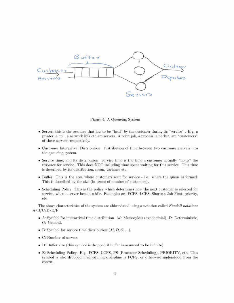
Figure 4: A Queueing System

• Server: this is the resource that has to be “held” by the customer during its “service” . E.g. aprinter, a cpu, a network link etc are servers. A print job, a process, a packet, are “customers”of these servers, respectively.

• Customer Interarrival Distribution: Distribution of time between two customer arrivals intothe queueing system.

• Service time, and its distribution: Service time is the time a customer actually “holds” theresource for service. This does NOT including time spent waiting for this service. This timeis described by its distribution, mean, variance etc.

• Buffer: This is the area where customers wait for service - i.e. where the queue is formed.This is described by the size (in terms of number of customers).

• Scheduling Policy: This is the policy which determines how the next customer is selected forservice, when a server becomes idle. Examples are FCFS, LCFS, Shortest Job First, priority,etc

The above characteristics of the system are abbreviated using a notation called Kendall notation:A/B/C/D/E/F

• A: Symbol for interarrival time distribution. M : Memoryless (exponential), D: Deterministic,G: General.

• B: Symbol for service time distribution (M,D,G . . .).

• C: Number of servers.

• D: Buffer size (this symbol is dropped if buffer is assumed to be infinite)

• E: Scheduling Policy. E.g. FCFS, LCFS, PS (Processor Scheduling), PRIORITY, etc. Thissymbol is also dropped if scheduling discipline is FCFS, or otherwise understood from thecontxt.

5

• F: Population. If the sources of the requests are modeled, then this denotes the number ofusers in a “request-response” cycle with the server. For open systems, population is implicitlyassumed to be infinite, so this part is also usually not written.

Examples of queuing systems expressed using this notation are:

• M/M/1: Single server exponentially distributed service time and interarrival time, infinitebuffer, FCFS, open system.

• M/G/1/20: Single server, exponentially distributed interarrival time, finite buffer of size 20,FCFS, open system.

• G/G/c/K: c servers, generally distributed service and interarrival time, finite buffer of size K,FCFS, open system.

The essential quantitative parameters of an open queueing system are:

• Request Arrival rate: λ requests/sec (Mean Interarrival time is 1λ .

• Service Rate (maximum rate at which one server can provide service): µ requests/sec.

• Average Service Time: τ = 1µ

• Sometimes, the variance of service time.

• Number of servers: c

• Buffer size: K

The metrics that we usually analyze and are dependent on the above parameters are:

Λ, Average Throughput : Number of requests completed per unit time (also called departurerate).

ρ, Average Server Utilization : (or just “utilization”): Fraction of time a server is busy. Formultiple servers, this is the average fraction over all the servers.

W , Average Waiting Time: Time spent in queue before service starts

R, Average Residence/System/Response Time: Waiting Time + Service Time

N , Average Number of customers in the system (including in service)

Q, Average Queue Length : Average number waiting in the queue

2.1 Observational/Operational Laws

Some relationships between parameters can be derived with simple intuitive analysis of a queueingsystem. Suppose we have a single server infinite buffer queueing system under observation.

Let

T Observation/measurement periodA Number of arrivals in time TC Number of completions/departures in time TB Total time that system was busy in time T

Assume that T is very large. Note that we do not make any assumptions about the distributionsof service time and inter-arrival time.

6

Then the following is obvious:

Arrival Rate λ =A

T

Throughput Λ =C

T

Mean Service Time τ =B

C

Utilization ρ =B

T

=B

C.C

T= τΛ

Here,ρ = Λτ

is called the Utilization Law is an important law in queueing systems.For a lossless system, where λ < µ, for a long observation period, the number of departures must

be almost equal to the number of arrivals, thus the throughput Λ = λ and ρ = λτ .Thus:

Throughput Λ = λ if λ < µ

= µ if λ ≥ µ

and

Utilization ρ = λτ if λ < µ

= 1 if λ ≥ µ

A single server lossless queueing system is said to be stable if λ < µ.Now consider a finite buffer system where request is dropped when buffer is full. Let pl be the

request loss probability (i.e. buffer full probability). Then

Λ = λ (1− pl) ∀λ ≥ 0

. andρ = λ (1− pl)τ ∀λ ≥ 0

.Thus, a finite buffer system is always stable. This is because as λ grows, pl also grows.For multiple server (c servers), infinite buffer, the throughput and server utilization is as follows:

Throughput Λ = λ if λ < cµ

= cµ if λ ≥ cµ

and

Utilization ρ =λτ

cif λ < cµ

= 1 if λ ≥ cµ

7

[Lecture 3: January 13th, 2015]

For multiple server (c servers), finite buffer, the throughput and server utilization remains is:

Λ = λ (1− pl) ∀λ ≥ 0

. and

ρ =λ (1− pl) τ

c∀λ ≥ 0

.

2.2 Asymptotic Analysis of Open Queues

The above queueing systems can also be analyzed for some limiting values without making use ofcomplicated “maths”. We primarily look at limiting values as the load (arrival rate in this case)goes either to zero, or to infinity.

In the analysis regarding waiting time and response time, we assume thet the service time distri-bution has the memoryless property . In continuous distributions only the exponential distributionhas this property. This property implies this: suppose we observe the server when it is busy, anda time u has elapsed in the current service. Let Y be the random variable denoting the remainingtime of service. Then Y has the same distribution (and hence the same mean) as the total servicetime distribution. Thus it is as if there is “no memory” of how much work has already been doneon this customer. Hence such a distribution is called memoryless. We will prove this propertymathematically when we do our mathematical background review.

G/G/1 G/G/c G/G/1/K G/G/c/KMetric λ → 0 λ →∞ λ → 0 λ →∞ λ → 0 λ →∞ λ → 0 λ →∞

Throughput 0 µ 0 c µ 0 µ 0 c µUtilization 0 1 0 1 0 1 0 1

Queue Length 0 ∞ 0 K 0 ∞ 0 KNumber in System 0 ∞ 0 K + 1 0 ∞ 0 K + c

Waiting Time 0 ∞ 0 Kτ 0 ∞ 0 Kc τ

Response Time 0 ∞ 0 (K + 1)τ 0 ∞ 0 (Kc + 1)τ

Question: where exactly are we using the memoryless property in the entries above?

2.3 Little’s Law

Consider any system through which customers traverse for service (see Figure 5). Consider the boxwith the boundary drawn in that system. Customers enter that box, get some service there andleave that region. Let R be the amount of time the customers spend inside that box. Let N be theaverage number of customers inside that box, and let Λ be the rate of “flow” of customers throughthat box (in other words, the throughput through that box).

Suppose further that the servers in this system are work conserving - i.e., they will not be idleif there is a customer in the queue, and work is not “lost” after it enters the system. Furthersuppose that the scheduling policy does not require knowledge of the service time requirement ofthe customers.

Then Little’s Law states that:N = ΛR (1)

8

Figure 5: Pictorial view of Little’s Law

Little’s Law is remarkable because at first glance it seems to do something non-intuitive. Forexample, if you imagine a queuing system whose average number in the system is known to be N ,and average service time is τ , the “intuitive” thing to do is to multiply τ by N +1 (arriving customersees N in the system on an average, will on an average need Nτ waiting time and then τ service timeto finish). Why doesn’t this reasoning work? It comes down again to the memorylessness property.In the reasoning where we arrive at (N + 1)τ , we assume that the mean of the remaining servicetime of the customer in service is also τ , which is not the case of service time is not memoryless.Hence this reasoning does not work.

This should imply that for a memoryless service time distribution, the intuitive reasoning shouldwork. In fact, it does. We will prove later that for an M/M/1 queue,

N =ρ

1− ρ

Now by the direct reasoning we get:

R = (N + 1)τ = (ρ

1− ρ+ 1)τ =

τ

1− ρ

By applying Little’s law we get:

R =N

λ=

ρ

1− ρ× 1

λ(2)

=τ

1− ρ

which is the same as we get with the “intuitive” reasoning.Various queueing theorists have their own way of intuitively understanding Little’ Law. Mor

Harchol-Balter explains that since Λ is the throughput, which is also the “departure rate”, theaverage inter-departure time is 1

Λ . This time can be interpreted as the effective time by the system

9

to complete one customer. So if there are average N customers in the system, the time required toprocess all of them is N × 1

Λ . This intuition may work or not work for you!Kleinrock explains the formula as follows: suppose we start with the average response time.

This is the average time each customer spends in the system. For stable lossless system, λ × R isthe number of customers that will arrive during this time and you could interpret it as the averagenumber of customers in the system.

[Lecture 4: January 16th, 2015]

2.3.1 A visual proof of Little’s Law

Consider a single server queueing system. Let us plot two curves on the same graph:

• A(t): Cummulative number of arrivals upto time t

• D(t): Cummulative number of departures upto time t

These curves will be as shown in Figure 6. Note that the two graphs are identical except howthe enclosed area is divided (“horizontal rectangles” vs “vertical” rectangles”).

Figure 6: Visual Proof of Little’s law

We prove Little’s Law by calculating the area enclosed in within the two plots above in two was:first by adding the areas of the “horizontal rectangles”, and then by adding the areas of the “verticalrectangles” and equating these two.

The width of the horizontal rectangles is the response time of the customer in the system. Theheight is 1. Let the number of arrivals (and number of departures) be A. Area by adding horizontalrectangles =

A∑i=1

(Ri × 1) =A∑

i=1

Ri

=

(∑Ai=1 Ri

A

)A

= RA

10

Here R =PA

i=1 Ri

A is the average response time.The height of the vertical rectangles is the number of customers in the system (because the

height is equal to the cumulative number of arrivals minus cumulative number of departures, so thisdifference should be what is left in the system). Denote these by Ni, for the ith rectangle. Thewidth is the time difference between the two consecutive events (arrival or departure), denoted byT1, T2, . . . , Tk, . . .. Note that this means that there are Ni customers in the system for Ti amount oftime.

Thus, the area is:

k∑i=1

Ni × Ti =

[k∑

i=1

Ni

(Ti

T

)]T

= NT

note that here Ti

T is the fraction of time that the number of customers in the system are Ni,therefore N =

∑ki=1 Ni

(Ti

T

)is average number of customers in the queueing system.

Equating two areas

RA = NT

N =A

TR

N = λR

2.4 Closed Queuing Systems

Closed queueing systems are models that arise when the sources of the requests are modeled explic-itly. An example of a closed system is one in which there is a a fixed number of users or clients eachof whom issues a request to the server, waits for a response, “thinks” for a while (e.g processes theresponse itself) and then issues the next request to the server.

A “canonical” one-server, and M user system is visualized as follows

Figure 7: Canonical Closed System

Let:

11

• Average think time be denoted by 1λ .

• Service rate be denoted by µ and average service time by τ = 1µ .

• Number of users be denoted by M

• Throughput= Λ, Server Response time = R, server utilization = ρ.

2.4.1 Canonical Closed System: Operational and Asymptotic Analysis

Just like for open queues, we can analyze this closed system to some extent, without needing to useadvanced mathematical models.

Some preliminary observations - since this is a closed system, it is important to realize that atequilibrium, the rate of requests flowing through the edges anywhere in this system is going to be thesame. e.g. the rate of request flow at points P, Q, and X, Y are the same at equilibrium. Specifically,the aggregate rate at which users issue requests = arrival rate at server = throughput at server =aggregate response rate at users.

How does one understand this? We must realize that the server and the users “modulate” eachother. E.g., what is the rate at which ONE USER issues requests? This is best understood bylooking at one user’s timeline.

Figure 8: User Timeline

It is immediately apparent from this timeline, that one user issues a request ever R + 1λ time.

Thus, an individual user’s request rate slows down as the server’s response time increases. (This isvery different from an open system.)

12

Now consider this:

Average request issue rate by 1 client =1

E[R] + 1λ

Total request arrival rate =M

E[R] + 1λ

Total throughput

Λ =M

R + 1λ

R =M

Λ− 1

λ

At high load, limM→∞

R =M

µ− 1

λ

At high load, limM→∞

R = Mτ − 1λ

At low load, limM→0

R = τ

Thus, the response time has two linear asymptotes. We still do not know enough to calculatethe response time for values of M between the asymptotes. But based on what we will learn later,we know that the response time curve looks like this:

Figure 9: Response Time vs Number of Users

The nature of this curve can be used to derive a very important metric for this system - thatof how many users can this system support? Note that the high load asymptote is reached whenserver utilization is close to 1. When the server utilization is 1, we say that the system is saturated.Since the system is essentially a “finite” system, it is still mathematically stable, but it is saturatedand adding more users just increases the response time, while does nothing to the throughput.

Thus the point at which or just before which the high load asymptote is reached should beconsidered as the maximum load this system can support. The shape of this curve can be exploitedto derive a heuristic that gives us this number as shown in the following figure.

The M∗ shown in the figure can be calculated as follows:

13

Low load asymptote: τHigh load asymptote: Mτ − 1

λ

Mτ − 1λ

= τ

Mτ = τ +1λ

M∗ = 1 +1λτ

= 1 +µ

λ

M∗ is called the “saturation number”.Note that the saturation number has a very intuitive explanation. First rewrite it as:

M∗ = 1 +thinktimeservicetime

This makes the number immediately clear: look at the server timeline shown here. Supposethe server has just finished serving a request from User 1 at time t1, then we know that User 1is expected to send his next request only after “thinktime” amount of time. In the “thinktime”amount of time, the server can process ‘

thinktimeservicetime

requests, one from one user each. From the figure, clearly, the number of “simultaneous users” thisserver can handle is 1+ thinktime/service time - which is the saturation we dervided!

Figure 10: Server Timeline

14

2.4.2 Closed System: Little’s Law

Little’s Law can be applied to a closed system if we visualize the “boundary” to which we have toapply Little’s Law as shown in this Figure:

Figure 11: Little’s Law for the Closed Queueing System

For us to apply Little’s Law we have to abstract the closed system as a system in which thereare a fixed number of requests M , that “circulate” through the system. The request is either at theserver or “at the client” (when the user is thinking). Thus, the average number of customers in thesystem is fixed at M .

What is the time through the region? Clearly it is : server response time + think time. Thus,we can derive the same equilibrium equation as we got earlier, by using Little’s Law:

M = Λ(

1λ

+ R

)

2.5 Queueing Networks

So far we have studied systems in which there is just one server to which a request has to go. Inreality though, a request may need to go through multiple queueing systems until it is completelyfinished. E.g. a request in a typical “multi-tier” Web application needs service from a Web Server,Database server, perhaps an Authentication server, etc before it is fully done.

Such systems are represented by queueing networks.

2.5.1 Closed Tandem Queuing Network

First, let us look at a simple queuing network as shown in the following figure. Here a request firstneeds service from Server 1, then from Server 2 and then is “done”. Queues in such a configurationare called tandem queues.

Let us carry out asymptotic analysis on this queueing system as done earlier. Suppose servicetime at Server 1 is τ1 and at Server 2 is τ2.

At M = 1:

15

Figure 12: Tandem Queues

Rsys = τ1 + τ2 (3)

Λ =1

1λ + τ1 + τ2

(4)

Applying Little’s Law at any user level M , we have:

M = Λ× (R1 + R2 +1λ

)

Let Rsys = R1 + R2 be the overall system response time. Then

Rsys =M

Λ− 1

λ

where R1, R2 are the response times at server 1 and 2 respectively. In case of the tandem queuingsystem, for large M , Λ → minµ1, µ2. That is, the maximum throughput will be whatever the slowerserver can support. We term this server the bottleneck server of the system.

Let µB = minµ1, µ2. Then for large M

Rsys =M

µB− 1

λ

We can apply Kleinrock’s saturation heuristic here also to find the maximum number of customersthe system can support.

Rlow = τ1 + τ2 = Rhigh =M∗

µB− 1

λ

M∗ = µB

[τ1 + τ2 +

1λ

]

16

2.6 Closed Queueing Networks - Mean Value Analysis

Now consider a general queuing network as shown in the figure below.//insert closed QN

Figure 13: Closed Queueing Network

In general we assume that there are m + 1 queuing stations - station 0 is the client node andstations 1 to m are service stations. In this queuing network, we assume that when a request isdone at a certain service station i, it goes to service station j with a probability pij . Note that inthis generalized closed queuing network, feedback is possible. That is, we can have pii > 0, meaningthat as soon as a request is done at station i, it may need service at the same station immediatelyagain, with probability pii. Feedback may also happen from another station - i.e. a request goesfrom station i to j and then back to i. Feedback results in a request needing multiple visits to astation before it is completed.

The probabilities pij determine the average number of visits a request makes to any station beforeit is completed. Let this average be denoted by vi. Thus vi is the average number of visits made bya request to station i before it leaves (i.e. goes back to the client node). This is also called the visitcount.

In the given figure, how do we calculate, say v1? We see every request issued by the client visitsserver 1 at least once. Also, every request that visits server 2 also visits Server 1. Thus it is fair tosay that

v1 = 1 + v2

.Conversely, we can see that a fraction p12 of requests that visit server 1 also visit server 2. Thus

v2 = p12 × v1

17

Solving the above equations shows:

v1 =1

1− p12

andv2 =

p12

1− p12

In general, visit count to station j is given by the following system of linear equations:

vi =M∑i=1

pij × vi, i = 1, 2, 3, . . .

Once visit counts are calculated, a very important quantity of a queuing network is defined,called the service demand. This is the total time over multiple visits that a request uses service froma server.

Thus service demand at station i is given by

Bi = vi × τi

For queuing networks, we can define two sets of metrics - one set at the ”system level” and oneset for each node i. Furthermore, it makes most sense to study these metrics as functions of the”load level” which is the number of users (or clients), M . Thus we have:

• Rsys(M), “System Response Time”: Time taken by a request from entering the server networkto leaving the server network. This is the complete request response time as ”experienced” bya user.

• Rcycle(M), “Cycle Time”: This is the time taken by a request to complete a cycle through theentire queueing network. Thus Rcycle = thinktime + Rsys.

• Λsys(M), “System Throughput”: The rate at which requests are completed, which will also beequal to the total rate at which M users issue requests to the system.

• Ri(M), “Node Response Time”: Response time at node i during one visit by a request. Notethat because a request visits station i on an average vi times, and each time spends Ri amountof time at server i.

Rsys(M) =M∑i=1

viRi(M)

• Λi(M), “Node throughput”: Request throughput at a node i, is given by

Λi(M) = vi × Λsys(M)

• Ni(M), “Average number of customers at node i: Note that

N0(M) + Ni(M) + . . . Nm(M) = M

• ρi(M), “Utilization at node i”. As usual,

ρi(M) = Λi(M)× τi

18

2.6.1 Asymptotic Analysis

As usual, let us start with analyzing the above metrics at low load (M = 1).The response time at low load is

Ri(1) = τi

andRsys(1) =

∑i

vi × τi

The throughput is given by the same reasoning as for the canonical system (this can be derivedboth by Little’s Law and by observing one user’s timeline).

Λsys(1) =1

1λ + Rsys(1)

The utilization of each service station is given by:

ρi(M) = (Λsys(M)× vi)× τi

This formula holds for M = 1 as well as M > 1.Expanding the above formula for M = 1, we can see that it can also be interpreted as the fraction

of time spent in the server i during the cycle of one request through the system (this logic worksonly when there is just one request in the server).

ρi(1) =viτi

thinktime +∑M

i=1 viτi

Also, for any M the Little’s Law equality for closed systems holds:

M = Λsys ×Rcycle

M = Λsys ×

[1λ

+M∑i=1

viRi

]Now let us consider the high load asymptotes, i.e., for large M .At what value does system throughput flatten out as M goes to infinity?The maximum rate at which the system completes the request will be determined by the most

“slowest” server in the system. Note that, in a queueing network, whether a server’s relative capacityis determined not only by its raw service rate (µi = 1

τi) but the rate at which it can complete requests,

which accounts for the average number of visits to a server.Consider a simple example of some sort of an office (a government office, or a bank) which has

multiple counters for serving customers. Suppose there the clerk at counter 1 needs an average of5 minutes to service a customer, but a customer needs an average of 3 visits on an average to thiscounter before his work in this office is complete. Suppose the clerk at counter 2 needs an averageof 10 minutes per customer, but each customer needs an average of only 1 visit to this counter. It isclear that the clerk at counter 1 has a “raw” service rate of 12 tasks per hour, but can fully processonly 4 customers per hour. On the other hand the clerk at counter 1 has a raw service rate of 6 tasksper hour, but can fully process 6 customers per hour. It should be obvious then that the customerprocessing capacity of this office is 4 customers per hour. Thus although the clerk at counter 2 was“slower” - he is not the one that is limiting the throughput of this office.

This discussion should lead you to the obvious conclusion. The maximum throughput possiblefor a queuing network is given by:

19

limM→∞

Λsys(M) =1

maxi viτi

Here maxi viτi is termed as the bottleneck service demand and the server with the maximumservice demand is termed the bottleneck server.

Let Bmax = maxi viτi be the bottleneck service demand.Then for large M ,

M ≈[

1λ + Rsys

]Bmax

Rsys(M) ≈ MBmax −1λ

Thus the high load asymptote of Rsys is linear with slope Bmax.You can apply Kleinrock’s saturation number derivation heuristic here also. We leave it to the

reader to prove that the saturation number by this heuristic is:

M∗ =1λ +

∑Mi=1 viτi

Bmax

Suppose we define µmin = 1Bmax

. That is, this is the maximum system throughput capacity ofthe queuing network. One can also define an even rougher heuristic where we approximate the wholenetwork as a single server with service rate of µmin. In that case, the saturation number is given by:

1 +µmin

λ

We leave it to the reader to think about how these two heuristics compare.

2.6.2 Mean Value Analysis

So far in most of our analysis we have only focussed on asymptotes, and on some other simple metricsthat can be derived without involving advanced mathematical models (e.g. stochastic processes).

It turns out that in case of Closed Queueing Networks, if we make use of a very useful theoremcalled the Sevcik-Mitrani Arrival Theorem, we can derive all metrics even for the “medium load”values of M (i.e neither too low, nor too high), with a very elegant and intuitive algorithm calledMean Value Analysis.

First, we must understand the Arrival Theorem. For this, we make use of all the metrics definedabove and one additional one:

• NAi (M): Average number of customers at node i as seen by an arriving request.

Thus, NAi (M) is a conditional average, based on this number as noted only at request arrival

times at i (and which does not include the arriving request). Ni(M) is an unconditional average ofthis number. In general, we do not expect NA

i (M) to be equal to Ni(M) - i.e. we do not expectconditional and unconditional averages to be the same.

[Imagine you note the number of students in a classroom at several uniformly and evenly sampledtimes of the day and take an average. Now suppose you take another average conditioned on thetime of the observation being between 6pm and 7pm. These two averages will certainly not be thesame].

The arrival theorem applies for certain types of queueing networks called Jackson networks.Closed Jackson networks are the kind of queuing networks we have described so far, with one moreconstraint: the service times and think time are exponentially distributed.

20

With this constraint, the arrival theorem (informally) states that, for a closed queuing networkwith number of users M , the average number of customers at node i that an arriving request sees, isthe unconditional average number of customers at node i, when the queueing network has one lesscustomer in the system.

In other words, the arrival theorem states that:

NAi (M) = Ni(M − 1)

.This equivalence suggests a very powerful way of solving the model - that of recursion (or itera-

tion). This method is called mean value analysis.Let us start with what we know.

• At M = 0, we know that Ni(0) = for all i. Thus, we have an intial value for the Ni’s. Now wewill assume that we know Ni(M − 1) and try to go step-by-step until we have derived Ni(M).Then our recursion will be properly defined.

• The arrival theorem tells us that at load level M , an arriving request at node i will see anaverage of Ni(M − 1) requests in front of it. Further more, service time is memoryless. Thus,the expected response time at all the service stations will be:

Ri(M) = [Ni(M − 1) + 1]× τi

• Now we can write Rsys as

Rsys(M) =M∑i=1

viRi(M)

• Once we know Rsys(M), we know Rcycle(M) = thinktime + Rsys(M). So we can calculateΛsys(M) by applying Little’s Law to the whole system:

Λsys(M) =M

Rcycle(M)

• Now that we know the system throughput, we can calculate node througput as

Λi(M) = vi × Λsys(M)

• Recall that we already calculated the per-visit node response time Ri(M) in the first stepitself. So we can apply Little’s Law at the node level:

Ni(M) = Λi(M)×Ri(M)

This completes the recursion.

In this way Mean Value Analysis (MVA) can be used to calculate performance metrics at all loadlevels M for a Jackson closed queueing network.

21

2.7 Summary

So far we learnt concepts and laws in queuing systems such as:

• The Kendall Notation

• The utilization law

• Asymptotic metrics for the M/M/c/K class of queues

• Calculating averages of all metrics for Jackson closed queuing networks using Mean ValueAnalysis. We had to understand Sevcik-Mitrani’s Arrival Theorem for this purpose.

• The importance of memorylessness in making some conclusions.

We still do not know, for example, what is the average response time of an M/M/1 queue. Weknow that N = λR and if we know N we can determine R. But how do we determine N (the averagenumber of customers in the system) ? It turns out that we need to determine the distribution of thenumber of customers in the queuing system to then find the average. And for this, the mathematicaltoolbox we need is of stochastic processes.

First, we need to refresh some probability basics needed for our purposes. The field of probabilityand statistics is vast, we will only revise those parts that we need.

3 Probability and Random Variables

Queuing systems analysis depends on a thorough understanding of random variables and theirdistribution functions. For that we need to understand basic probability. So, before we go torandom variables, let us first quickly do some warm-up exercises in probability.

3.1 Simple Probability Models

Example 1: Let bit error rate/probability (b.e.r.) on a link be e, then what is the proba-bility that a packet of length L bits is correctly transmitted? Assume:

(a) All bits need to be correct.Solution:P[packet is correct] = P[all bits correct] =(1− e)L

This assumes that bit errors are independent.

(b) Error correcting code can correct 2 bit errors.Solution:P[packet is correct = P[≤ 2 bits in error]γ = P[0 bit error] + P[1 bit error] + P[2 bit error]γ = (1− e)2 + Le(1− e)L−1 + LC2e

2(1− e)L−2

(c) Suppose packet can go on one of two links with b.e.r. e1, e2 respectively. What is theprobability of succesful transmission?Solution:P[packet goes on link1] = p1

P[packet goes on link2] = p2

22

From case(b), we have:γ1 ... success on link1γ2 ... success on link2

A : packet is successfulB1 : Link1 is usedB2 : Link2 is used

P [A|B1] = γ1 (this is conditional probability)P [A|B2] = γ2

P [A] = P [A|B1] + P [A|B2] = γ1P1 + γ2P2

This is theorem of total probability.

Definition of conditional probability:

P [A|B] =P [A ∩B]

P [B]

Definition of total probability:Let S = B1, B2, . . . , Bn be the event space where,B1, B2, . . . , Bn are mutually exclusive and exhaustive events.Then, by law of total probability, we have,

P [A] =n∑

i=1

P (A|Bi) · P (Bi)

Bayes’ Theorem The event space can be viewed as a collection of Mutually exclusive andCollectively exhaustive events. Depending on our intuition or assumptions we can have a priorestimate of the events which can be termed as Prior probability. Given that an event occuredin the random experiment the probabilities for the events under consideration will change. Thisprobability can be termed as the Posterior probability. Bayes theorem helps in determining theposterior probability given some prior information of the events.

Let the event space consists of Bj mutually exculsive and collectively exhaustive events. Knowingthe prior probabilities and a event A occured the posterior probabilities can be calculated by:

P (Bj |A) =P (A|Bj)P (Bj)∑i P (A|Bi)P (Bi)

Example:Suppose, in the two-link case, the packet arrived successfully. What is the probability that it

came on link1?Solution:

P (Bj |A) =P (A ∩Bj)

P (A)=

P (A ∩Bj)∑i P (A|Bi)P (Bi)

=P (A|Bj)P (Bj)∑i P (A|Bi)P (Bi)

23

P[Link1 | packet is succesful] :

P (B1|A) =(

P (A|B1)P (B1)γ1P1 + γ2P2

)

Law of diminishing returns:

P[server is up] = r = 0.9

2 Server system :

P[system is up] = P[at least one server is up]r = 1 - P[both servers are down]r = 1 - (1− r)2

For an n-server parallel system, system is up when at least one server is up.Rserver = 1− (1− r)n

3.2 Efficiency of ALOHA

3.2.1 Pure ALOHA

NN*p*(1 − p)

N − 1(1− p)

No Transmission

should be there

Figure 14: Pure ALOHA

Lets do a “quick and dirty” probababilistic analysis of ALOHA. For the purposes of our analysislet us assume all packets are of equal size, and transmission time is unit time. Suppose the probabilityof a station transmitting in this unit time is p and the number of stations is N .

Note that this analysis is a bit “hand-wavy” and inaccurate. But it is popular and acceptable asa first rough model. .

What is the expected throughput of such a system? e.g. How many successful packetstransmitted per unit time? Since transmission time is the unit, this is really just the probability ofsuccessful transmission in the channel. Thus,Prob[successful transmission]= Prob[no transmission in previous unit slot] × Prob[no other transmission in this slot]

S = (1− p)N ·Np(1− p)N−1

24

S = Np(1− p)2N−1

For N stations, what should be the load per station, that maximizes the throughput? We cantry to guess this intutively. If there are N stations, one expects that if each one’s probability oftransmission at any time is 1

N , that feels like a “full and fair share” that should mazimize thethroughput.

Formally, the probability of transmission that maximumizes throughput is given by:

dS

dp= N(1− p)2N−1 −Np(2n− 1)(1− p)2N−2 = 0

p =1

2N

Smax =12

(1− 1

2N

)2N−1

Thus, note that our analysis tells us that our expectation was not met. Stations need to producemuch lesser load than we hoped, to maximize network throughput of pure ALOHA.

Now, as N increases, throughput decreases. The limiting throughput is:

limN→∞

S =12e∼ 0.18 = 18%

See the corresponding spreadsheet to understand this behaviour better and play with the pa-rameters.

3.2.2 Slotted ALOHA

N*p*(1 − p)N − 1

Figure 15: Slotted ALOHA

It is clear from the previous analysis that the throughput is reduced because transmissions fromthe previous “slot” can also collide with the current transmission. Slotted ALOHA improves thisby actually dividing time into slots, and requiring that stations transmit only at the beginning of aslot. In this case,

P[successful transmission] = P[max. 1 transmission in the slot]

S = Np(1− p)N−1

The per-station load that maximimizes success probability is given by

dS

dp= N(1− p)N−1 + Np(N − 1)(1− p)N−2 = 0,

25

Thus, highest success rate is at p = 1N . Thus slotted ALOHA meets our expectation. At this

value of p,

S =(

1− 1N

)N−1

limN→∞

S =1e∼ 0.37 = 37%

We can see that this is twice of the throughput achievable by pure ALOHA.This was just an illustration of using simple probabilistic methods to analyze protocol perfor-

mance. We will now move on to study random variables and probability distributions.

3.3 Random Variables

Random variables are results of random experiments - that is experiments that can have random,unpredictable outcomes. Formally, a Random Variable is a function that maps a “sample space” toset of real numbers. A sample space is the set of possible outcomes of an experiment.

E.g. suppose the experiment is of sending a packet across a link. The outcome is a successful orunsuccessful transmission. We define a random variable X as a function which maps success to thenumber 1 and failure with the number 0.In practice, though when we talk about random variables,we do not use a “function” notation. In the above example, conventionally we can say that “X is arandom variable that takes value 1 when the packet transmits successfully, and 0 if the transmissionfails.”.

There are two types of random variables (r.v.): discrete, and continuous. Discrete randomvariables take discrete values, while continues random variables take continues values.

3.3.1 Discrete Random Variables illustrated with a Go-back-N ARQ System

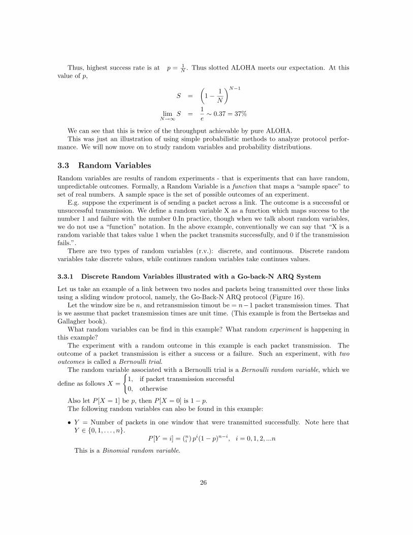
Let us take an example of a link between two nodes and packets being transmitted over these linksusing a sliding window protocol, namely, the Go-Back-N ARQ protocol (Figure 16).

Let the window size be n, and retransmission timout be = n−1 packet transmission times. Thatis we assume that packet transmission times are unit time. (This example is from the Bertsekas andGallagher book).

What random variables can be find in this example? What random experiment is happening inthis example?

The experiment with a random outcome in this example is each packet transmission. Theoutcome of a packet transmission is either a success or a failure. Such an experiment, with twooutcomes is called a Bernoulli trial.

The random variable associated with a Bernoulli trial is a Bernoulli random variable, which we

define as follows X =

{1, if packet transmission successful0, otherwise

Also let P [X = 1] be p, then P [X = 0] is 1− p.The following random variables can also be found in this example:

• Y = Number of packets in one window that were transmitted successfully. Note here thatY ∈ {0, 1, . . . , n}.

P [Y = i] = (ni ) pi(1− p)n−i, i = 0, 1, 2, ...n

This is a Binomial random variable.

26

Ret

rans

mis

sion

Tim

er

12

Sender Receiver

n

Figure 16: Go-back-n ARQ system

27

• N = Number of transmissions required to send a packet correctly. N ∈ {1, 2, 3, ...}. Here,exactly k transmissions will be required if k − 1 transmission fail followed by one successfultransmission. Thus,

P [N = k] = (1− p)k−1p

.

This is the Geometric random variable.

• NR = Number of re-transmissions requried to send a packet correctly. In other words, numberof failures before the packet was transmitted correctly. The packet may succeed in the firsttransmission itself, so N ∈ {0, 1, 2, 3..} and

P [NR = k] = (1− p)kp

• D = total time required for a successful transmission of a packet (including time retransmis-sions). Let’s call it packet transfer delay. Note that here we start counting the time requiredfor a packet to be sent, only when all the packets before it in the window have been successfullysent (removed from the packet buffer).

If the first transmission is a success, the packet needs only 1 time unit.

If first transmission is a loss, this will be discovered after the retransmission timer expires -i.e. n− 1 time units after transmission. Then we need one more time unit to transmit. Thus,if two transmissions are required, time taken is 1 + n− 1 + 1 = n + 1.

If k transmissions are a failure, and time required will be kn + 1. Thus,

P (D = 1 + kn) = (1− p)kp for k = 0, 1, 2, . . .

This is not a well-known distribution and has no name.

• If Z = the size of the sliding window as observed at any random time, it is fair to assume thatit will be of any size between 1 and n with equal probability. This is the Discrete UniformDistribution. Thus

P [X = k] =1n

, k = 1, 2, . . . , n

.

There is one more important distribution that we can associate with this example. This distri-bution needs a slightly involved derivation.

Suppose we want to ask the question: how many packets are likely to arrive at the link fortransmission, in a given timeframe? This question characterizes the arrival process and the “load”on the link.

A common set of assumptions that characterize the arrival process are as follows:

• Packets arrive into the source in an infinitesimal interval 4t with probability λ4t, whereλ > 0. (Note that λ can be greater than 1. We assume that ∆t is small enough that theproduct is a probability. )

• P[two or more arrivals in 4t] → 0.

• Arrivals in different intervals are independent of each other.

28

Under these assumptions, what is the probability that k jobs arrive in time interval (0, t)? LetNA(t) be the random variable denoting the number of jobs arriving in (0, t). Then we want to knowP [NA = k]. We proceed as follows: Divide time (0, t) into n slots such that t

n = 4t.

P [k jobs in (0, t)] = exactly k out of n slots have job arrivals= (n

k ) (λ4t)k(1− λ4t)n−k

= (nk ) (λ

t

n)k(1− λ

t

n)n−k

=(

n!(n− k)!nk

)(λt)k

k!

[(1− λt

n

)−n/λt]−λt

(1− λt

n

)kSince the assumption is that∆tis small, wehave

P [k jobs in (0, t)] = limn→∞

k terms︷ ︸︸ ︷n · n− 1 · · · (n− k + 1)

n · n · · ·n[· · · ]

=(λt)k

klim

n→∞

[(1− λt

n

)−n/λt]−λt

(1− λt

n

)k=

(λt)k

k

[limn→∞

(1− λt

n

)−n/λt]−λt

(1− limn→∞

λtn

)klim

n→∞=

(λt)k

ke−λt

∼ Poisson(λt)

Let λt = α.

NA ∼ Poisson(α)

⇒ P [NA = k] =αke−α

k!

3.4 Important Distributions of Discrete Random Variables

We now define some terms about random variables and their distributions semi-formally, and sum-marize the discrete distributions that we saw above.

The Probability Mass Function PX(x) of a random variable X gives the probability of occu-rance of each value of the random variable.

PX(X = x) −→ [0, 1]

wherex ∈ Sample Space(S)

Some properties of a PMF are:

• 0 ≤ PX(x) ≤ 1

29

•∑

x PX(x) = 1

The Cumulative Distribution Function (CDF) FX(t) of a random variable X representsthe cumulative probability of X till point (x = t).

FX(t) = P (x ≤ t) =∑x≤t

PX(x)

where t ∈ R and t can be continuous.Example: X = {1, 2, 3, 4, 5, 6, 7, 8, 9, 10}

PX(x) =110

FX(8.6) =810

Some properties of a CDF, also referred-to as simply the Distribution Function, are the following:

• 0 ≤ FX(t) ≤ 1

• Monotonically nondecreasing.

• limt→∞ FX(t) = 1

• limt→−∞ FX(t) = 0

Now we summarize the pmfs and CDFs of some well-known distributions. For each distribution,we mention what is described as the parameter of the distribution.

3.4.1 Bernoulli PMF

Parameter: p

X ∈ {0, 1}

PX(1) = p PX(0) = 1− p

FX(t) =

0, for t < 01− p, for 0 ≤ t < 11, for t ≥ 1

3.4.2 Binomial PMF

Parameters: n, p

X −→ Number of successes i in n Bernoulli Trials

X = 0, 1, 2, . . . , n

P (success) = p

PX(i) =(

n

i

)pi(1− p)n−i

30

The Poisson PMF can be used as a convenient approximation to the binomial PMF when n islarge and p is small (that is n →∞ and p → 0, in such a way that np → α):(

n

i

)pi(1− p)n−i ≈ e−ααi

i!

where α = np

Example: Bit errors in a packet of length L (packet size in bits is large, and error probability isvery small).

3.4.3 Geometric Distribution

Parameter: p

X −→ Number of trials upto and includng a success

X = 1, 2, 3, . . . ,∞

P (success) = p

PX(i) = (1− p)i−1p

CDF is the probability that we will need less than or equal to i trials. This is one minus theprobability of needing more than i trials. This happens w.p. 1− p)i, thus:

FX(i) = 1− (1− p)i

Geometric distribution has the memoryless property. This is apparent if you think like this:Suppose you have been tossing a coin to get a head, but have gotten 20 tails in a row. What is theprobability that you will need 20 more tosses to get a head? Think for a second and you will knowthat this probability is the same as if you had just started tossing the coin - i.e. the experiment hasno memory of number of trials already done.

Formal proof of Markov Property (memorylessness):

X is the total number of trials for success. The additional number of trials required for success,after i unsuccessful trials is denoted by random variable Z. Note that if we know that i trials wereunsuccessful, that means we know that X has to be strictly greater than i. This we know, so it is agiven condition. Thus finding the probability of Z = k means we need to find the probability thatX = k + i, given that X > i

P [Z = k] = P [X = k + i | X > i]

=P [X = k + i]

P [X > i]

=(1− p)k+i−1p

(1− p)i

= (1− p)k−1p

⇒ Z → Geom(p)

31

Example: Bit error rate on a channel is b. Bit errors are independent. In a packet, the first 10bits have come error-free. What is the probability that the first bit error is seen at exactly the kthbit after these 10 bits?

Solution:By memoryless property, Z ∼ Geom(b)

P [Z = k] = (1− b)k−1b

3.4.4 Modified Geometric Distribution

Parameter: p

X −→ Number of failures before a success

X = 0, 1, 2, . . . ,∞

PX(i) = (1− p)ip

Example: while not B do S;X : # of times S is executed

P (B = true) = p

P (X = k) = (1− p)kp

X ∼ ModGeom(p)P [X > k] is probability that there are more than k failures, that is there are at least k+1 failures

= (1− p)k+1.

FX(k) = P [X <= k] = 1− P [X > k] = 1− (1− p)k+1

3.4.5 Poission

Parameter: α

PX(i) =e−ααi

i!

FX(i) =k=i∑k=0

e−ααk

k!

3.4.6 Uniform

Parameter: N

X = {x1, x2, x3, . . . , xN}

PX(xi) =1N

FX(t) =t

N

32

3.4.7 Constant / Deterministic

Parameter: c

X = c

PX(x) =

{1, for x = c

0, for x 6= c

FX(t) =

{0, for t < c

1, for t ≥ c

3.4.8 Indicator Random Variable

X = 1 if event A and X = 0 if event A.

3.5 Expectation

The expectation (mean), denoted by E[X], of a random variable X is defined as:

E[X] =∑

i

xip(xi) X → discrete random variable (5)

3.5.1 Uniform

X = {1, 2, . . . , n} pX(x) = 1n

E[X] =n∑

i=1

i

n=

n + 12

3.5.2 Bernoulli pmf

Parameter: pE[X] = p (6)

3.5.3 Binomial

Parameters: n, p

E[X] = np (7)

E[∑

i

Xi] =∑

i

E[Xi] (Xis need not be independent) (8)

3.5.4 Geometric

Parameter: ppX(i) = (1− p)i−1p

E[X] =1p

(prove as homework) (9)

33

3.5.5 Modified Geometric

Parameter: ppX(i) = (1− p)ip

E[X] =1− p

p(prove as homework) (10)

3.5.6 Poisson

Parameter: α

pX(k) =αke−α

k!

E[X] =∞∑

k=0

αke−α

k!

= αe−α∞∑

k=1

αk−1

(k − 1)!

= αe−αeα

E[X] = α (11)

3.6 Superposition and splitting of Poisson Arrivals

Suppose (open) arrivals to a queue come from two sources - each of which are Poisson. Then themerged arrival stream is also Poisson. This is because the sum of two Poisson random variables isalso Poisson. Recall that “arrivals are Poisson” is short for saying that the number of arrivals intime (0, t) has Poisson distribution with parameter λt where λ is the “rate” parameter.

Let X ∼ Poisson(α1) and Y ∼ Poisson(α2) and let Z = X + Y .What is the probability that Z = k? If we know that say, Y = j, then this is the probability

that Z = k − j. Thus, using the Law of Total Probability we can write:

pZ(k) =k∑

j=0

pX(k − j)pY (j) (12)

=k∑

j=0

e−α1αk−j1

(k − j)!e−α2αj

2

j!

=e−(α1+α2)

k!

k∑j=0

k!(k − j)!j!

αk−j1 αj

2

=e−(α1+α2)

k!(α1 + α2)k Binomial Expansiona

Thus Z ∼ Poisson(α1 + α2).Now suppose that an arrival stream which is Poisson is split probabilistically. That is, say, an

arrival goes to server 1 with probabilty p and server 2 with probability 1− p.Let N denote the number of arrivals in (0, t) in the original stream. Then N ∼ Poisson(λt). Let

α = λt.

34

Let N1 denote the number of arrivals going to server 1 in time (0, t). Then what is the probabilitythat N1 = k?

We can condition this on N . If we know that N = j, then what is the probability that N1 = k.It is 0 if k > j and otherwise it is the probability that k out of j arrivals went to server 1. Thus

pN1(k) =∞∑

j=k

pN1|N (k|j)pN (j) (13)

=∞∑

j=k

(j

k

)pk(1− p)j−k e−ααj

j!

=e−α(αp)k

k!

∞∑j=k

αj−k(1− p)j−k

(j − k)!

=e−α(αp)k

k!eα(1−p)

=e−αp(αp)k

k!

3.7 Continuous Random Variables

Figure 17: CDF and pdf of continuous random variables

Random variables such as processing time, interarrival time may not always described by discretevalues - they are better described by continuous random variables (c.r.vs).

For a continuous random variable, say X, the probability of taking a certain value is 0. i.e.P [X = c] = 0 for any specific value c. This is because the r.v. can take such a large (infinite)

set of values, that the probability of taking any one value is essentially zero.Thus, for c.r.v. we can only find probabilities of the r.v. being in a certain range. Thus, for

continuous random variables, we define a cummulative distribution function, sometimes called justthe “distribution function”:

FX(x) = P [X <= x] −∞ < x < ∞

35

The CDF has the same properties as the discrete CDF(Figure 17):

0 ≤ FX(x) ≤ 1,−∞ < x < ∞lim

x→−∞= 0

limx→−∞

= 0

and FX(x) is a monotone non-decreasing function.Consider a small range (x, x + dx). We know that

P [x < X < x + dx] = F (x + dx)− F (x)

.Thus, for a small dx, this quantity captures the probability of values close to x. This intuition

is represented by the probability density function (pdf) of a continuous random variable, which isgiven by

fX(x) =dFX(x)

dx

Thus fX(x)dx approximates the probability of values in the range (x, x + dx). Note that fX(x)itself is not a probability.

A PDF is a function that must satisy the following properties:

fX(x) ≥ 0, −∞ < x < ∞∫ ∞

−∞fX(x)dx = 1

It follows from the above definitions that

FX(x) =∫ x

−∞fX(t)dt

P [a < X <= b] = FX(b)− FX(a) =∫ b

a

fX(t)dt

It follows that

P [X = c] =∫ c

c

fX(t)dt = 0

In other words, for continuous r.v.s, the area under the curve of a pdf function is the probability- “pieces” of this area will be probabilities, not the values. So, although P [X = c] = 0, P [c < X <c+ δc] is defined and can be non-zero. Also, while the value of the pdf is not a probability, it is goodindicator of ranges of the random variable that are more likely then the other. E.g. in Figure 17,values in a small range around x are more likely than in a range around x2 (this is because the areaslice under fX(x) will be be larger than the area slice under fX(x2)).

36

3.7.1 Exponential Distribution

This is a distribution which has some unique properties, which make it a very useful distribution inmodeling.

If a random variable X has a distribution given by

F (x) = 1− e−λx, X ≥ 0, λ > 0

then X is said to have the exponential distribution with parameter λ. This distribution is alsodenoted by EXP (λ).

The pdf of such a random variable is given by:

f(x) = λe−λx

The exponential distribution has the memoryless property. An example of this is as follows:suppose you are at a phonebooth while somebody is on the phone. Suppose this person has beenalready talking for 10 minutes. What is the probability that he will hold the phone for 10 moreminutes? If the call holding time distribution is exponential (which it often is), the probabilityof talking for 10 hold minutes is the same as if the person had just started talking - i.e. it is“memoryless”. Let us prove this mathematically:

Let X be the random variable denoting the holding time. Suppose we know that X > t (“personhas already been talking for t time units”). Let Y be the remaining time. Then X = Y + t.

P [Y ≤ y] = P [X ≤ y + t|X > t]

=P [X ≤ y + tX > t]

P [X > t]

=P [t < X ≤ y + t]

P [X > t]

=F (y + t)− F (t)

[1− F (t)]

=(1− e−λ(y+t))− (1− e−λt)

e−λt

=e−λt[1− e−λy]

e−λt

= 1− e−λy

3.7.2 Relationship of Poisson distribution and Exponential Distributions

Poisson distribution can be derived in the context of arrivals of requests to a system. Suppose thatnumber of arrivals Nm to a system in an interval (0, t] follows Poisson distribution.

⇒ P [N = k] =(λt)ke−(λt)

k!What is the distribution of the interarrival time (X)? We can pose this question as what is

P [X > t]. In words, if one arrival happenned at time 0, then the probability that there has been noarrival till at least time t is that there were 0 arrivals is the interval (0, t]. Thus P [X > t] = P [N =0] = e−(λt). ThusP [X < t] = 1− e−(λt). Thus X has EXP (λ) distribution.

Poisson and Exponential distributions complement each other. When the arrivals are Poisson, theinter-arrival time is Exponential. If arrivals are Poisson with rate λ, interarrival time is exponentiallydistributed with mean 1/λ.

37

3.7.3 Order Statistics

If we are given a set of random variables X1, X2, . . . , Xn, we often need to find the distribution ofthe minimum, or the maximum of these variables. Thus let Y and Z be random variables defined as

Y = mini{Xi}

andZ = max

i{Xi}

. Then if we know FXi(t)’s, can we determine FY (t) and FZ(t)?

It is clear that Y , the minimum, will be greater than some y if all Xi’s are greater than y. Thus:

P [Y ≥ y] = P [X1 ≥ y]P [X2 ≥ y] . . . P [Xn ≥ y]

which means1− FY (y) = Πn

i=1(1− FXi(y))

FY (y) = 1−Πni=1(1− FXi(y))

Similarly, Z, the maximum will be less than some y if all Xi’s are less than y. Thus:

P [Z ≤ y] = P [X1 ≤ y]P [X2 ≤ y] . . . P [Xn ≤ y]

which meansFZ(y) = Πn

i=1FXi(y)

3.7.4 Minimum of Exponentially Distributed Random Variables

Let Xi’s be random variables, each with distribution EXP (λi). Let Y = mini{Xi}. Then

FY (y) = 1−Πni=1(1− FXi(y))

= 1−Πni=1e

−λiy

= 1− e−(P

i λi)y

Thus the minimum is EXP (∑

i λi).

3.8 Distributions of Continuous Random Variables

Hypoexponential Distribution

Sum of exponential stages.Consider X = Y + Z, where Y → EXP(λ1) and Z → EXP(λ2).Then X → HYPO(λ1, λ2) and it has pdf:

f(t) =λ1λ2

λ2 − λ1(e−λ1t − e−λ2t), t > 0

Expectation:Parameters: λ1, λ2, . . . , λn

E[X] =n∑

i=1

1λi

38

Erlang Distribution

Special case of HYPO where all stages have identical distribution.

f(t) =λrtr−1e−λt

(r − 1)!, t > 0, λ > 0, r = 1, 2, . . .

Represented as ERLANG(n, λ) which is quivalent to sum of n EXP(λ).Expectation:Parameters: n, λ

E[X] =n

λ

Hyperexponential Distribution

Mixture of exponential phases where one and only one of the alternative phases is chosen. The pdfof a 2-way hyperexponential random variable is:

f(t) = α1λ1e−λ1t + α2λ2e

−λ2t

Expectation:Parameters: αi, λi where i = 1, 2, . . . , n

E[X] =n∑

i=1

αi

λi

//notes about squared coeff of variation to be added

4 A first principles analysis of the M/M/1 queue

Consider a system with one server and infinite queue capacity. The arrivals are Poisson with rate λand the service time is exponentially distributed with rate µ.

Let N(t) = number of jobs in the system at time t. We call N(t) the state of the system at timet.

Suppose N(t) = k. Then what is N(t+∆t)? (Where ∆t is an infinitesimally small time interval.)In the small interval ∆t, we can have an arrival, or a departure. We know by the definition

of Poisson arrivals that an arrival happens in a small interval ∆t with probability λ∆t. Also twoarrivals cannot happen in this interval.

If k ≥ 1, then what is the probability of a departure in an interval ∆t? Since service timedistribution is EXP (µ), this probability is:

1− e−µ∆t = 1− (1− µ∆t +(µ∆t)2

2!+ . . .)

= (µ∆t− (µ∆t)2

2!+ . . .)

≈ µ∆t (14)

We can similarly argue that the probability of two departures in a small interval is negligible.Pr[ Arrival in ∆t ] is λ∆t.Pr[ Departure in ∆t ] is µ∆t.Pr[ Arrival & Departure in ∆t ] is λµ(∆t)2 ≈ 0.

39

Then N(t + ∆t) = k ifA: N(t) = k and no jobs arrive/depart in (t, t + ∆t] w.p. 1− λ∆t− µ∆tB: N(t) = k − 1 and 1 job arrives in (t, t + ∆t] w.p. λ∆tC: N(t) = k + 1 and 1 job departs in (t, t + ∆t] w.p. µ∆t

Unconditional Probability:Let Pk(t) = P [N(t) = k]. Then

Pk(t + ∆t) = Pk(t) + [λPk−1(t)− (λ + µ)Pk(t) + µPk+1(t)]∆t

The rate of change of probability = lim∆t→0

Pk(t + ∆t)− Pk(t)∆t

=dPk(t)

dtdPk(t)

dt= λPk−1(t)− (λ + µ)Pk(t) + µPk+1(t)

We are often interested in the state of the system as t → ∞. Under certain conditions,limt→∞ Pk(t) exists and converges to a unique value πk. This probability is called the steady stateprobability of the system being in state k.

If steady-state exists, limt→∞dPk(t)

dt → 0.

(λ + µ)πk = λπk−1 + µπk+1 , k = 1, 2, · · ·λπ0 = µπ1

(λ + µ)π1 = λπ0 + µπ2

(λ + µ)π2 = λπ1 + µπ3

...

πk =λ

µπk−1

Letλ

µ= ρ.

Then the above equations can be written as

π1 =λ

µπ0 = ρπ0

π2 =λ

µπ1 = ρπ1

π3 =λ

µπ2 = ρπ2

...πk = ρπk−1

= ρ · ρπk−2

...

= ρkπ0 , k = 1, 2, · · · ,∞

40

Since∞∑

k=0

πk = 1

∞∑k=0

ρkπ0 = 1

⇒ π0 =1∑∞

k=0 ρk

π0 = 1− ρ

ρ = 1− π0 . . .Probability that the server is busy

πk = ρk · (1− ρ)

Thus πk is the “Modified Geometric” distribution with parameter (1− ρ)

If N is the number of jobs in the system at steady state, then

E[N ] =1− (1− ρ)

1− ρ=

ρ

1− ρ= Avg. Queue length

ByLitte′sLaw :

E[R] =E[N ]

λ=

1µ(1− ρ)

= Avg. Response time

Thus, using a first principles approach, we can calculate various metrics of the M/M/1 queueingsystem.

However {N(t)|t ≥ 0} is actually an example of a special kind of stochastic process. We willnow study Stochastic Processes, and see how those methodologies based on stochastic processes canmake the above analysis very straightforward.

5 Stochastic Processes

A stochastic process is a family of random variables {X(t)|t ∈ T} defined on a given probabilityspace, indexed by the parameter t, where t ∈ T . Values of X(t) define the state space and theparameter t is time in many cases. Based on the combinations of state and parameter types, wehave the following classification of stochastic processes:

ParameterState

Discrete Continuous

Disrete Discrete-parameter chain Discrete-paremeter continuous state processContinuous Continuous-parameter chain Continuous-parameter continuous state process

Examples from queueing systems:DPDS: Nk: number of jobs in the system seen by the kth arrivalDPCS: waiting time of the kth customerCPDS: N(t) number of jobs in the system at time tCPCS: remaining work in the system at time t

41

5.1 Markov Process

{X(t)|t ∈ T} is called a Markov process if for any t0 < t1 < t2 < · · · < tn < tP [X(t) ≤ x|X(tn) = xn, · · ·X(t1) = x1, X(t0) = x0] = P [X(t) ≤ x|X(tn) = xn]

The interpretation of the above property is as follows: if we label time tn as “current”, thentimes t0, t1, ...tn−1 are the “past” and time t is the “future”. Also X(t) typically represents a system“state” that is changing over time. Then the above property says that for a Markov process, thefuture state of the system depends only on the current state of the system, not on the path takento come to the current state of the system.

We implicitly used this property when we did the first-principles analysis of M/M/1 queue. Wepredicted the value of N(t + ∆t) based only the value of N(t) not on N(t−∆t) and older states.

Further if P [X(t) ≤ x|X(tn) = xn] = P [X(t− tn + u) ≤ x|X(u) = xn],the Markov proces is said to be time-homogenous. This means that if a process is in state xn now,then probability of being in some state x, some v time units later, depends only on xn and the timedifference v, not on the actual current time.

What exactly does this mean? This means that the system parameters which determine thebehaviour of the stochastic process are not changing over time, and hence we do not have to keeptrack of how much time has “elapsed” since the “beginning”. Recall again that our N(t) of theM/M/1 queue had this property. We wrote the transition probabilities in terms only of the timedifference, which was ∆t. In the “RHS” of the expressions of the state transition probabilities, thereis only ∆t, and no t.

If, on the other hand, for example, the arrival rate was time dependent (λ(t)), the correspondingstochastic process would not be time-homogeneous.

A continuous-time, discrete state stochastic process can only have the time-homogeneous Markovproperty if the distribution of all the events that lead to state changes of the stochastic process areexponential. Only in such a case can a discrete state capture all the information required to predictthe future.

Then the time-homogeneous Markov property of a process implies that the distribution of timespent in a state is exponential. Only in this distribution, can the time remaining in a certain statehave the same distribution, no matter how much time the system has already spent in that state.

A stochastic process which has discrete states is called a chain. Thus a continuous time, discretestate Markov process is commonly termed as Continuous Time Markov Chain (CTMC).

5.2 Analysis of time-homogeneous CTMCs

Consider a time-homogeneous CTMC {X(t)|t ≥ 0}. Then we know that the time spent in a statehas exponential distribution. It follows that the duration of all “events” that cause state changesmust be exponentially distributed. The basic goal of analysis of a CTMC is to determine:

Pk(t) = P [X(t) = k], the probability that the system is in state k at time t.

which in vector form is denoted by P(t) = [P0(t), P1(t), . . .]A time-homogeneous CTMC (henceforth, we call this just “CTMC”) is characterized by the

following:

• The definition of a state space of the system. For this analysis, let the state space be{0, 1, 2, · · · }, without loss of generality.

• The transition rate qij at which the CTMC changes state from i to j. In other words, qij isthe parameter of the exponential distribution of the time for going from state i to state j.

42

• An initial state probability vector P(0) = [P0(0), P1(0), . . .], which gives the probability thatthe system was in state k at time t = 0.

The CTMC is often represented pictorially with a state-transition diagram.An example is {N(t)|t ≥ 0} from Section 4, which denoted the number of customers in an M/M/1

queue at time t. This CTMC is characterized by:

• State space S = {0, 1, 2, . . .}.

• Transition Rates:

– qi,i+1 = λ,∀i = 0, 1, 2, . . .

– qi,i−1 = µ,∀i = 1, 2, 3, . . .

– qij = 0 otherwise.

• P(0) = [1, 0, 0, . . .]. That is, we can assume that at the beginning the system is empty, withprobability 1.

Now, we can follow a derivation very similar to the one in Section 4, to arrive at a generalequation for P(t) in terms of the parameters of the CTMC, namely P(0) and qij ’s.

Then, consider an infinitesimal small interval ∆t. What is the probability that the system willbe in state j at time t + ∆t? That is

What is Pj(t + ∆t) = P [X(t + ∆t) = j]?

The CTMC can be in state j at time t + ∆t if:

• X(t) = i, i 6= j and a transition from i to j happened in a small interval ∆t. Recall that sincethe distribution of the time for this transition is EXP (qij), we can use the same reasoning aswe used in Section 4, Equation 14 and state that this will happen with probability qij∆t.

• X(t) = j and no state transition happened in the interval ∆t. Now note that in state j manysimultaneous transitions are “in progress” - the transition from state j to a state k is inprogress with distribution EXP (qjk). Thus the time to the first transition which will achievea state change, is a minimum of all transition times, and thus, the distribution is

EXP (∑

k,k∈S,k 6=j

qjj)

Thus, the probability that there will be a transition out of state j in time ∆t is (see Section 4)

(∑

k,k∈S,k 6=j

qjk)∆t

Therefore, the probability that there is no transition is:

1−∑

k,k∈S,k 6=j

qjk∆t

Thus, the unconditional probability Pk(t + ∆t) = P [X(t + ∆t) = j] is given by the law of totalprobability:

Pj(t + ∆t) =∑

i,i∈S,i 6=j

qij∆t Pi(t) + (1−∑

k,k∈S,k 6=j

qjk∆t) Pj(t)

Pj(t + ∆t)− Pj(t)∆t

=∑

i,i∈S,i 6=j

qijPi(t)−∑

k,k∈S,k 6=j

qjktPj(t)

43

Defineqj =

∑k,k∈S,k 6=j

qjk

.Then, taking limit of ∆t tending to zero on both sides, we have:

dPj(t)dt

=∑

i,i∈S,i 6=j

qijPi(t)− qjPj(t) (15)

Now, if we define the matrix Q as follows:

Qij = qij , i 6= j

Qjj = −qj

(16)

Then the above equation can be written in matrix form as:

dP(t)dt

= P(t)Q

The solution to the above equation (stating without proof) is

P(t) = P(0)eQt

where

eQt = I +∞∑

n=1

Qntn

n!

Again, we are interested in the system state probabilities as t →∞. For this, we state the followingdefinition and theorem:

A CTMC is said to be irreducible if every state is reachable from every other state.

Theorem: For an irreducible CTMC the following limits always exist and are independent ofthe initial state i.

πj = limt→∞

Pj(t),∀j ∈ S

If the underlying system is stable, then as t → ∞, the CTMC is said to achieve statisticalequilibrium and the limiting probabilities are called the steady state probabilities of the CTMC.

At steady state, Pj(t) becomes constant, hence its derivative becomes zero. Taking limits ast →∞ on Equation 15, we get

0 =∑i 6=j

πiqij − πjqj

⇒ πjqj =∑i 6=j

πiqij

⇒ rate out of state j = rate in to state j

These are called steady state balance equations of a CTMC. We can solve for the steady stateprobability vector π = [π0, π1, . . .] by using the above balance equations, and the normalizing con-dition:

πQ = 0 and∑j∈S

πj = 1

44

6 Markovian queueing systems analysis using CTMCs

Now we study a series of Markovian queues using CTMCs.

6.1 M/M/1 queue

Figure 18: M/M/1 state transition diagram

Here, the state is the number of customers in the queue. Thus S = {0, 1, 2, . . .}.The transition rates were defined in the above section.The CTMC corresponding to the M/M/1

queue can be drawn as shown in Figure 18.Note that the balance equations can also be written by drawing the CTMC as a graph, and then

making “cuts” in the graph that divide the graph into two parts. Then equate the average “flow”in one direction of the cut to the average “flow” in the other direction of the cut.

E.g. for the M/M/1 queue, if the cut as shown in Figure 18, then the average steady state flowfrom left to right is λπi−1 and from right to left is µπi. Thus we have:

λπi−1 = µπi

which is the same as we got using the “first principles analysis”. The rest of the analysis followssimilarly.

Note that the sum of the infinite series in these derivations converges only under certain condi-tions. The CTMC achieves a steady state only under these conditions. The underlying system isthen considered stable. We term these conditions the stability criteria for the system. For M/M/1queue, the stability criterion is

λ < µ

6.2 M/M/c/∞ queue

Here we have multiple servers and a single queue. m is the number of servers, each with EXP (µ)service time. The total capacity of the system is cµ requests per unit time.

Interarrival ∼ EXP(λ)The state of the system here is also the number of customers in the queueing system. Thus

S = {0, 1, 2, . . .}.

45

Figure 19: M/M/c state transition diagram (substitute m by c in the diagram above

Now consider a state i < c. What are the “events in progress” in this state?There is one EXP (λ) arrival that can happen.If the arrival happens first, the state will be i + 1.This happens at the “rate” λ.There are i “services” or “departures” in progress. The distribution of time to the first departure isEXP (iµ), since it is the minumum of the i service times each of which are EXP (µ). A departurewill change the state to i− 1.

Now consider a state i ≥ c. Here, there are more than c customers in the system, but atmax c servers can be busy serving customers. Thus, distribution of time to the next departure isEXP (mµ).

Figure 19 shows these state transitions. We can again write the balance equations by doing the“cuts” as shown.

λπj−1 = jµπj ∀1 ≤ j ≤ c

λπc+j−1 = cµπc+j ∀j ≥ 0

Let ρ = λcµ .

For 1 ≤ j ≤ c, this implies

πj = λjµπj−1

π1 = λµπ0 = cρπ0

π2 = λ2µπ1 = cρ

2 π1 = (cρ)2

2! π0

π3 = λ3µπ2 = cρ

3 π2 = (cρ)3

3! π0

...πj = cρ

j πj−1

= cρj · cρ

j−1πj−2

...πj = (cρ)j

j! π0 (17)

46

For c + j ≥ c, this implies

πc+j = λcµπc+j−1, j ≥ 0

πc+1 = λcµπc = ρπc

πc+2 = λcµπc+1 = ρ2πc

πc+3 = λcµπc+2 = ρπc+2 = ρ3πc

...πc+j = ρπc+j−1

= ρ · ρπc+j−2

...πc+j = ρjπc = ccρc+j

c! π0 (18)

Now, we can determine π0 using:∞∑

j=0

πj = 1

We have,

c−1∑j=0

πj +∞∑

j=0

πc+j = 1

c−1∑j=0

(cρ)j

j!π0 +

∞∑j=0

ρjπc = 1

c−1∑j=0

(cρ)j

j!π0 +

(cρ)c

c!π0

∞∑j=0

ρj = 1

c−1∑j=0

(cρ)j

j!π0 +

(cρ)c

c!π0

1− ρ= 1 if ρ < 1

π0 =

c−1∑j=0

(cρ)j

j!+

(cρ)c

c!1

1− ρ

−1

if ρ < 1 (19)

We note here that we have discussed the notion of stability earlier but we can see its mathematicaldefinition here. The queuing system is stable if the pj ’s above are well-defined. In the above, thesteady state probabilities exist and are well-defined if ρ < 1. Thus, the Stability criterion for thisqueue is λ < cµ.

Let us now derive some performance metrics. The throughput and utilization for this system aregiven as usual, we do not need Markov chain analysis for that.(Throughput of the queueing systemis λ when λ < mµ and mµ when λ ≥ mµ. Utilization is ρ).

But we now have the distribution of N : the number of customers in the system at steady state.Recall that what we have just calculated is

limt→∞

P [N(t) = j] = πj

.

47

Then the Expectation of N is;’

E[N ] =∞∑

j=0

jπj

The expected response time at steady state is then

E[R] =E[N ]

λ

Let M denote the number of busy servers at steady state. Then

E[M ] =c−1∑j=0

jπj +∞∑

j=c

cπj

Let NQ denote the number of customers in the buffer (waiting). Then

E[NQ] =∞∑

j=c+1

(j − c)πj

The expected waiting time, W, at steady state is then

E[W ] =E[W ]

λ

We can also find the probability of “queueing”, that is the probability that an arriving requesthas to wait in the buffer (i.e. has non-zero waiting time).

For this we first need to understand a result called PASTA: “Poisson Arrivals See Time Averages”.This result states that when arrivals are Poisson, the probability of an arriving customer seeing kcustomers in the system is just the unconditional state probability πk. (Recall the example given inclass of a D/D/1 queue. Complete this example to show how this is not true in general.)

The request has to queue if it sees c or more servers busy. Thus, using PASTA,

P[queuing] =∞∑

j=c

πj

6.3 M/M/c/K queue

The state transition diagram for this queuing system is also almost the same as M/M/c- except thatthe “last” state is c + K after which an arrival is dropped, hence the state does not change.

48

The analysis for the this queue is almost the same as for M/M/c, however we get

c−1∑j=0

(cρ)j

j!π0 +

(cρ)c

c!π0

K∑j=0

ρj = 1 (20)

π0 =

c−1∑j=0

(cρ)j

j!+

(cρ)c

c!

K∑j=0

ρj

−1

(21)

π0 =

c−1∑j=0

(cρ)j

j!+

(cρ)c

c!(K + 1)

−1

if ρ = 1 (22)

π0 =

c−1∑j=0

(cρ)j

j!+

(cρ)c

c!1− ρK+1

1− ρ

−1

ifρ 6= 1 (23)

This expression is well-defined for all values of ρ, thus there is no stability criterion for this queue.Let us now calculate the performance metrics of the system. Note that ρ here is not the utiliza-

tion.The probability of arriving request being dropped is given by the probability that an arriving

request sees the buffer FULL:

ploss = πc+K by PASTA

.Thus throughput is given by:

Λ = λ(1− πc+K)

.Then, average server utilization is given by:

Λcµ

Then the Expectation of N is;’

E[N ] =c+K∑j=0

jπj

The expected response time at steady state is then

E[R] =E[N ]

ΛThe metrics E[M ], E[NQ], E[W ] can be found similarly as for M/M/c queue (with sums going

to c + K instead of ∞).

6.4 Cyclic Queuing Model of a Multiprogramming system

So far we have learnt that closed queuing networks are used to model systems in which a fixed(small) set of users are in a closed request-response loop with a server system. However, there isone more scenario where closed queuing networks can be used as an abstraction which faithfullycaptures the behaviour of the system.

49

Consider a server, e.g. a multi-threaded Web server that is configured with a fixed number ofthreads, running on a computer. A thread in this server will typically circulate between using theCPU, the disk or the network several times before the request is complete.Thus, the thread is a“customer” in a queuing network comprising of the CPU, Disk and the Network. Now suppose thatwe want to analyze this system during its peak hour, when we know that all the threads of the Webserver are always busy, and arriving requests have to queue for getting an idle thread. In the peakhour of usage, the following is expected to happen: a thread starts on a request on the CPU, visitsCPU/disk/network multiple times, visits CPU one last time, and then the request is finished. Assoon as this request is finished, since the load is high, there will be another request in the queue,and the thread will immediately pick up this request from the queue.

Now if we assume that these requests are statistically similar, then picking up the next requestfrom the queue is mathematically equivalent to the previous request re-joining the CPU queue. Thusit is as if there is a fixed number of customers (threads) circulating “forever” between these threequeuing stations: CPU, Disk, Network.

This is the abstraction that leads us to model this system as a closed queuing network. Note thatin this network there is no “think station”. The threads are “always busy” circulating between thehardware resources. The hardware resources, on the other hand may or may not be busy, dependingon the number of threads in the system, and the relative service demands of the various resources.

The figure shows the queuing network model corresponding to a simple CPU-IO system. Weassume that the thread starts on a request at the CPU. After leaving the CPU, it may be done,with probability p - which means it re-joins the CPU with probability p, or goes to the I/O queuewith probability q = 1− p. After doing some I/O the thread always returns to the CPU queue.

This queuing network can be solved by the MVA algorithm that we have learnt earlier. But itcan also be modeled directly using CTMCs. In this section, we will analyze it using CTMCs.

50

51

52

53

54

7 Open Queuing networks

Figure 20: Open Queueing Network

So far we have studied closed queuing networks, where clients who issue requests are modeledexplicitly. However, sometimes the number of simultaneous users of the system are very large (e.g.50,000), and it is not feasible to model the clients explicitly. Furthermore, if their think time is alsolarge, then it can be shown that the arrival process as seen at the server entry point starts lookinglike a Poisson process. Thus, it makes sense to “ignore the clients” and focus on the request arrivals.Figure 20 shows an example open queuing network.

Open queueing network are queueing networks where “external arrivals” are possible to everynode. A request entering the queuing network may visit the queuing stations several times beforeexiting. Note that the total number of requests circulating in an open queueing network is not fixed.

For an open QN, as usual, we want to ask the usual questions:

• What is the maximum throughput that this network is capable of ?

• Which is the bottleneck server?

• For a certain arrival rate, what is the system throughput? What are the server utilizations?

55

• For a certain arrival rate, what is the system response time of a request?

A little bit of thought will make it clear to you that the first two questions are independent ofwhether the queuing network is being modeled as closed or open. The number of visits a requestmakes to a station can be determined in the same way as was done for closed queueing networks.This also implies that the service demand at each node is calculated in the same way. This in turndetermines the bottleneck system throughput as the reciprocal of the maximum service demand.

What remains then is the last two questions. Let us first consider throughput, when the totalarrival rate to the system is λ. It is clear that the asymptote of this as arrival rate increases is thebottleneck system throughput, which was defined above. Now, if we assume infinite buffers at allnodes, it follows that as long as the arrival rate is lesser than this value, the throughput will beequal to arrival rate. Thus

Λsys = λ if λ < Λmax (24)= Λmax if λ ≥ Λmax (25)

(26)

where if vi is the average visit count at node i and E[Bi] is the expected service demand at nodei, then

Λmax =1

maxi E[Bi]

To find the average response time (or the number of customers at the queue), one could ask thequestion - “can these queues be evaluated in isolation”? Then we can simply apply the formulas forthe single server queuing systems that we know!

We see now that this can in fact, be done. First, we consider a simple example.

7.1 Two-Server Tandem Queuing network

Figure 21: Open Tandem Queueing Network

Consider a two-stage tandem network as shown in the Figure 21. The sysetm consists of twonodes with respective service rates µ0 and µ1. The external arrival is Poisson with rate λ. Theservice-time distribution at both nodes is exponential.

Since all interevent tmes are exponentially distributed, the system can be modeled as a Contin-uous Time Markov chain, whose states are specified by pairs (k0, k1), k0 ≥ 0, k1 ≥ 0, where k0 andk0 are number of jobs at server 0 and server 1 respectively.

The state-transition diagram corresponding to a generic state of this CTMC is shown in Figurex.

56

Let P (k0, k1) be the joint probability of k0 jobs at the first server and k1 jobs at the next server,in the steady state. Equating the rates of flow into and out of the state, we obtain the followingbalance equations:

(µ0 + µ1 + λ)P (k0, k1) = µ0P (k0 + 1, k1 − 1) + µ1P (k0, k1 + 1) + λP (k0 − 1, k1), k0 > 0, k1 > 0.

For the boundary states, we have:

(µ0 + λ)P (k0, 0) = µ1P (k0, 1) + λP (k0 − 1, 0), k0 > 0(µ0 + λ)P (0, k1) = µ0P (1, k1 − 1) + µ1P (0, k1 + 1), k1 > 0

λP (0, 0) = µ1P (0, 1)

The normalization is provided by: ∑k0≥0

∑k1≥0

P (k0, k1) = 1

It is easily shown by direct substitution that the following equation is the soluton to the abovebalance equations:

P (k0, k1) = (1− ρ0)ρk00 (1− ρ1)ρk1

1 = P (k0)P(k1)

where, ρ0 = λ/µ0 and ρ1 = λ/µ1, and P (k0) and P (k1) are the steady state probabilities ofhaving k0 an k1 customers at queue 1 and 2 respectively, if each queue was an independent M/M/1queue. Thus, the tandem queues in the figure behave like 2 independent M/M/1 queues. The jointdistribution is the product of individual distributions.

Expected number of jobs in the system is:

E[N ] =ρ0

1− ρ0+

ρ1

1− ρ1

Average Response time is:

E[R] =E[N ]

λ

7.2 Product Form (Jackson) Open Queuing Networks

It turns out that even if queuing networks have splitting, joining and feedback, the steady statejoint distribution of jobs at each queueing station is a product of the marginal distribution of jobsat each queue. In fact, Jackson’s theorem can be stated as follows:

Consider an open queuing network with (m + 1) stations, where the ith station consists of ci

exponential servers, i = 0, 1, . . . ,m each with mean service time of 1/µi seconds. External Poissonsources contribute γi jobs/second to the average rate of arrival to the ith station.

Then the total external arrival rate to the queueing network is given as:

λ =m∑

i=0

γi

.

57

The routing matrix is given by :

X = [xij ]

and is such that the matrix power series∞∑

k=0

Xk

converges. (This property implies that after some cycles, a job must leave the open queuingnetwork.)

Then, according to Jackson’s result, each queue behaves like an independent M/M/ci queueingsystem with service rate of µi and effective arrival rate λi as given by:

λi = γi +m∑

j=0

xjiλj , i = 0, 1, . . . ,m

Also, for each queue i, we need λi < ciµi

This means that if πi(ki), is the probability of having ki jobs at station i, then

π(k0, k1, . . . , km) = π0(k0)π1(k1) . . . πm(km)

E.g. if ci = 1 for all the queues, then:

π(k0, k1, . . . , km) = Πmi=0ρ

kii (1− ρi)

where ρi = λi

µi

7.3 Example

Figure 22: Open Queuing Network Example

58

Consider the system as shown in figure 22. Let the service requirement per visit of the indi-vidual servers be τWS , τA1, τA2, τD1, τD2. Let arrivals be Poisson with rate λ and service times beexponential.

We find the average number of visits per server, i.e. VW , VA1, VA2, VD1, VD2 as:

VA1 = PWA1VW + PA1D1VA1

VA2 = PWA2VW + PA2D2VA2

VD1 = PA1D1VA1

VD2 = PA2D2VA2

VW =1

PW0

(27)

By back-substitution, we get:

VA1 = PWA1VW + PA1D1VA1 = PWA1VW /(1− PA1D1) = PWA1/(PW0(1− PA1D1))VA2 = PWA2VW + PA2D2VA2 = PWA2VW /(1− PA2D2) = PWA2/(PW0(1− PA2D2))

VD1 = PA1D1VA1 =PA1D1PWA1

PQ0(1− PA1D1)

VD2 = PA2D2VA2 =PA2D2PWA2

PQ0(1− PA2D2)

VW =1

PW0

(28)

The effective arrival rates at individual servers in terms of (request/sec)*(visits/request) wouldbe:

λW = VW λ

λA1 = VA1λ

λA2 = VA2λ

λD1 = VD1λ

λD2 = VD2λ

(29)

The average service demand at each of the servers would be:

E[BW ] = VW τW

E[BA1] = VA1τA1

E[BA2] = VA2τA2

E[BD1] = VD1τD1

E[BD2] = VD2τD2

(30)

The maximum among the above will be the bottleneck service demand, and the correspondingserver will be the bottleneck server. The maximum throughput supportable will be the reciprocal ofthe bottleneck service demand.

59

Response time on individual servers would be:

E[RW ] =(

τW

1− λW τW

)E[RA1] =

(τA1

1− λA1τA1

)E[RA2] =

(τA2

1− λA2τA2

)E[RD1] =

(τD1

1− λD1τD1

)E[RD2] =

(τD2

1− λD2τD2

)(31)

Total Response time for a request entering the system is the summation of total time taken ateach of these servers. i.e.

E[R] =∑

i

No. of visits to server ‘i’ * Response time at server ‘i’ per visit

=∑

i

Vi ∗ E[Ri]

=∑

i

viτi

1− λiτi

=∑

i

viτi

1− λviτi

=∑

i

Bi

1− λBi(32)

where Bi = viτi is the average service demand at server i.We can see from the way the above expression is written that the average response time in

this network can also be expressed as the sum of response times at an equivalent tandem queuingnetwork where we have one server corresponding to each of the servers in the original queuingnetwork, whose average service time is equal to the average service demand of the original queuingnetwork (Figure 23).

Figure 23: Equivalent Tandem Queuing Network to the Open Queuing Network in Figure 22. Arrival rateis λ and average service time = average total service demand at each station in the original network.

8 Discrete Time Markov Chains

A Markov process with discrete state space and discrete parameter space is known as a Discrete-TimeMarkov Chain (DTMC).

60

Let {Xn | n = 0, 1, 2, . . .} represent the state of the system at time step n. Xn takes discretevalues. If the following property is satisfied:

P (Xn = in | X0 = i0, X1 = i1, . . . , Xn−1 = in−1) = P (Xn = in | Xn−1 = in−1)

then {Xn | n = 0, 1, 2, . . .} is a Discrete Time Markov Chain. As seen earlier in CTMCs the aboveproperty means that the future (Xn) depends only on the present state of the system (Xn−1 = in−1,)and is independent of its past (X0 = i0, X1 = i1, . . . , Xn−2 = in−2 .

Let pjk(m,n) = P (Xn = k | Xm = j), 0 ≤ m ≤ n denote the probabililty that the DTMCmakes a transition from state j at step m to state k at step n. Then a DTMC is homegeneous ifpjk(m,n) = P [Xn = k | Xm = j] = P [Xn−m = k |X0 = j].

In other words, for homegeneous DTMCs, the number of time steps elapsed “from the beginning”also does not matter. The only thing that matters is the state the system is in at the current step.Thus, for homogeneous Markov chains:

pjk(n) = P (Xm+n = k | Xm = j)

That is, the probability in the RHS is a function only of the time step difference n.A DTMC is completely described by:

• A state space S. Without loss of generality we assume this to be S = {0, 1, 2, . . .}

• Initial state probabilities i.e. P{X0 = i} ∀ i.

• One-step transition probabilities: pjk = pjk(1) = P (Xn = k | Xn−1 = j), n ≥ 1

For a DTMC, the matrix P = [pij ] must be a stochastic matrix, i.e.∑

j pij = 1, ∀ iGiven this information, we are generally interested in the probability that the DTMC is in state

j at time step n, denoted by pj(n) = P (Xn = j).We can find this using a special case of the Chapman-Kolmogorov equation:

pj(n) =∑

i

pi(n− 1)pij (33)

Let p(n) = [p0(n), p1(n), . . . , pj(n), . . .]. Then this can be written as

p(n) = p(n− 1)P.

= p(n− 2)P.P...= p(0)Pn

Limiting State Probabilities In the condition that the Markov chain is irreducible, aperiodic,recurrent and non-null, the following limit exists and is independent of initial probability:

vj = limn→∞

pj(n), j = 0, 1, . . .

Here

• Irreducible means that every state is reachable from every other state.

61

• Aperiodic means that there is no periodic state in the DTMC. A state is periodic if the numberof steps in which one can return to the state after leaving it is a multiple of an integer greaterthan 1. For an irreducible DTMC, either all states are periodic, or all are aperiodic.

• Recurrent non-null roughly captures the property of “stability”. We know from our study ofCTMCs that limits of probabilities do not exist if the system is not stable. We do not definethis phrase formally here, but note the requirement that if the DTMC is infinite-state, stabilityproperty will have to be met for limits to exist.

Now we have, from Equation 33:

limn→∞

pj(n) = limn→∞

∑i

pi(n− 1)pij

⇒ vj =∑

i

vipij

v = vP

where∑

i

vi = 1 and vj ≥ 0

Thus when limits exist they can be found by solving the above set of linear equations.Now we will look at a few examples of modeling using DTMCs.

8.1 Page Hit rate analysis

A program’s address space typically consists of continuous pages represented by the indices1, 2, . . . , n. For the purpose of studying a program’s reference behaviour, it can be representedby the reference string w = x1, x2, . . . , xt, . . . . Successive references are assumed to form a sequenceof independent, identically distributed random variables with the pmf:

P (Xt = i) = βi, 1 ≤ i ≤ n;n∑

i=1

βi = 1.

The number of page frames is in most cases smaller than the number of pages referenced. Let ndenote the number of pages and m denote the number of page frames available. Clearly, 1 ≤ m ≤ n.The internal state of the paging algorithm at time t denoted by q(t), is an ordered list of them pages currently in main memory. We assume that on a page fault, the rightmost page in theordered list q(t) will be replaced. On the page hit, there is no replacement but the list q(t) isupdated to q(t + 1), reflecting the new replacement priorities. It is clear that the sequence of statesq(0), . . . , q(n), . . . , q(t), . . . forms a discrete-time homogeneous Markov chain with the state spaceconsisting of n!/(n−m)! permutations over 1, 2, . . . , n.

LRU paging algorithm

As an example, consider the LRU paging algorithm with n = 3 and m = 2. q(t) = (i, j) impliesthat the page indexed i was more reently used than page indexed j, and, therefore, page j will bethe candidate for replacement. The state space I is given by:

I = (1, 2), (2, 1), (1, 3), (3, 1), (2, 3), (3, 2)

Let the current state q(t) = (i, j). Then the next state q(t + 1) takes one of the following values:

q(t + 1) =

(i, j), if xt+1 = i,with associated probability βi,

(j, i), if xt+1 = j, with associated probability βj ,

(k, i), if xt+1 = k, k 6= i, k 6= j, with associated probability βk.

62

Then the transition probaility matrix P is given by:

P =

β1 β2 0 β3 0 0β1 β2 0 0 0 β3

0 β2 β1 β3 0 00 0 β1 β3 β2 0β1 0 0 0 β2 β3

0 0 β1 0 β2 β3

It can be verified that the avove Markov chain is irreducible and aperiodic; hence a unique

steady-state probability vector v exists. This vector is obtained by solving the system of equations:

v = vP, and∑(i,j)

v(i,j) = 1 (34)

Solving this system of equations, we get:

v(i,j) =βiβj

1− βi

A page fault occurs in state (i, j), provided that a page other than i or j is referenced. Theassociated conditional probabiity of this event is 1 − βi − βj ; we hence regard r(i,j) = 1 − βi − βj

to state (i, j). The steady-state page fault probability is then given by:

E[Z] = F (LRU) =∑

(i,j)∈I

(1− βi − βj)βiβj

1− βi

8.2 More precise model of Slotted ALOHA

There are m nodes sending packets on a channel using a slotted ALOHA-type protocol. The basicmechanism of an ALOHA protocol is to just try to send a packet at a slot boundary. If it collides,the station tries it again with some probability.

• n are ‘backlogged’, i.e nodes which tried to send a packet, unsuccessfully

• m− n ’not backlogegd’, i.e nodes which do not have packets to send

Assumptions:

• Slot time is unit time

• First transmission: Arrivals to a station in a slot are Poisson(λ/m)

• Retransmission: A backlogged node retransmits with probability qr

• Stations have no buffer, so arrivals to backlogged nodes are dropped

Probability that an unbacklogged station has a packet to transmit in a slot= P[arrivals in previous slot] = 1− e−λ/m = qa

P[ i backlogged nodes transmit in a slot ] = Qr(i, n) =(ni

)qir(1− qr)n−i

P[ i unbacklogged node first transmit ] = Qa(i, n) =(m−n

i

)qia(1− qa)m−n−i

We define a DTMC: number of backlogged users the end of a slot intervals. Now if this numberis n at the end of an interval k, what can its value be at the end of the next interval k + 1?

63

• n− 1: This can be if one backlogged user has a successful transmission, which will be if thereis exactly 1 backlogged transmission and no unbacklogged transmission

• n: The number of backlogged remains the same if either

– Exactly one unbacklogged transmits, and 0 backlogged transmits.

– Zero unbacklogged transmit, and two or more backlogged transmit

– zero backlogged and zero unbacklogged transmit

• n + 1: The number will increase by one if exactly one unbacklogged transmits, and at leastone or more backlogged transmit

• n + i, i ≥ 2: This will happen if exactly i unbacklogged transmit, and any number ofbacklogged transmit.

The corresponding one-step transition probabilities are:pn,n−1 = Qa(0, n) ·Qr(1, n)pn,n = Qa(1, n)Qr(0, n) + Qa(0, n)[1−Qr(1, n)]pn,n+1 = Qa(1, n)[1−Qr(0, n)]pn,n+i = Qa(i, n) 2 ≤ i ≤ m− n

Now we can solve for steady-state probabilities by solving:

v = vP,∑

vi = 1

where P = [Pij ]Now the expected number of backlogged nodes is: E[backlogged nodes] =

∑ni=0 ivi

If you apply Little’s law to a “box” which contains all the stations that are trying to transmit,then the delay through this box is given by:[ ∑n

i=0 ivi

Throughput

]

The throughput is the number of packet being transmitted successfully per unit time. Since theunit time is the slot time, this is number of packets being transmitted successfully per slot. Sinceonly one packet can be transmitted per slot, this is the same as the probability of the slot.

We first find the conditional probability of successful transmission given that there are n back-logged nodes.

64

Psucc(n) = Qa(1, n)Qr(0, n) + Qa(0, n)Qr(1, n)

= (m− n)qa(1− qa)m−n−1(1− qr)n + (1− qa)m−nnqr(1− qr)n−1

= (1− qa)m−n−1(1− qr)n−1[(m− n)qa(1− qr) + (1− qa)nqr]for small qa and qr =

= (1− qa)m−n(1− qr)n[(m− n)qa − (m− n)qaqr + n(1− qa)qr]

= (1− qa)m−n(1− qr)n[(m− n)qa −mqaqr + nqr]

= e(m−n)qaenqr [(m− n)qa + nqr]

= [(1− x)y = e−xy for x small]

= G(n)e−G(n)

whereG(n) = nqr + (m− n)qa

The unconditional probability of successful transmission is:

Psucc =∑

n

vnPsucc(n)

Throughput =Successful transmission per unit time = 1.Psucc + 0.(1− Psucc) = Psucc

9 M/G/1 queuing system

This is a single-server queuing system whose arrival process is Poisson with the average arrival rateλ. The job service times are independent and identically distributed with some distribution functionFB and pdf fB , which need not be exponential. Jobs are scheduled for service in their order ofarrival; that is, scheduling is FCFS.

Let N(t) denote the number of jobs in the system at time t. If N(t) ≥ 1, then a job is inservice, and since the general service time distribution need not be memoryless, besides N(t), wealso require knowledge of time spent by the job in service in order to predict the future behaviourof the system. It follows that the stochastic process N(t)|t ≥ 0 is NOT a Markov chain.

The trick to capture this system as a Markov chain is to observe it in a way that does not“interrupt” a service in progress. We do this by observing the system at times of departure of jobs.Let Xn denote the number of jobs in the system just after the departure of the n job. This is adiscrete-state, discrete-time stochastic process. But is it a Markov chain? It will be if we can saysomething about Xn+1 if only Xn is known.

See Figure ??. First suppose that Xn = 0; that is, the nth departure left the server idle. Whatstate can the (n+1)th departure leave the server in, and under what events? Note that the (n+1)thdeparture happens after the (n+1)th arrival. So after the nth departure, some time will elapse untilan arrival, and then after one service time, there will be the (n + 1)th departure. This is when wewill observe the system. Thus note that we will observe the system after an arrival and a departure- in other words, we are given that there was an arrival, and a depature after that arrival. Thus,the number of jobs in the system left behind after the departure will depend only on how many jobsarrived to the server during the (n + 1) job was being served.

Xn+1 will be zero, if no arrivals come during the (n + 1)th service. Xn+1 will be k, if k arrivalscome during the (n + 1)th service.

65

Let Yn+1 = No. of arrivals during (n + 1)thserviceNow, if Xn = i > 0 then that means the nth departure left the server busy with i jobs in the

system. The next departure will be exactly after one service time and we will observe the systemjust after this departure. How many jobs will be left in the system? Well, one less since one job hasleft, and k more, if k arrive during the service of the (n+1)th job. Thus Xn+1 will be Xn−1+Yn+1.

To summarize:

Xn+1 = Yn+1, if Xn = 0

Xn+1 = Xn − 1 + Yn+1, if Xn > 0

Let

P [Yn+1] = aj

and

Pij = P [Xn+1 = j|Xn = i]

ThenPij = P [Xn − 1 + Yn+1 = j|Xn = i] if i > 0

Pij = P [Yn+1 = j − i + 1|Xn = i] = aj−i+1 if j ≥ i− 1

P0j = P [Yn+1 = j] = aj , if i = 0

Thus, the one-step transition probability matrix can be written as:

P =

a0 a1 a2 a3 · · ·a0 a1 a2 a3 · · ·0 a0 a1 a2 · · ·0 0 a0 a1 · · ·0 0 0 a0 · · ·· · · · · · ·

(35)

Now let us consider the case where G = D, that is when service time distribution is deterministic.Let this service time be τ .

Then aj = Probability that there are j arrivals during one service is easily found, since arrivalsare Poisson with rate λ.

aj =(λτ)je−λτ

j!

Thus, for this case we can solve the DTMC equations for v, and find the steady-state probabilitiesof there being k jobs in the system at departure epochs.

However, how do we get the unconditional probability distribution of jobs in the system? Turnsout that for Poisson arrivals, the unconditional distribution is also the distribution at departureepochs (stating without proof). Thus, we have what we want.

66

9.1 M/G/1 waiting time using mean residual time approach

We could solve the DTMC equations precisely, and get the expected number of jobs in the system,apply Little’s Law and then get response time. But instead, we will use an interesting and elegantderivation to get the waiting time directly - by using the reasoning of mean residual time.

Some definitions:Wi : waiting tme of ith customer

Ti : Residual service time seen by the ith customerSi : Service time of ith customerNi : Number of customers found in queue by the ith customer

Wi = Ti + Si−1 + Si−2 + · · ·+ Si−Ni

E[Wi] = W = T + E[N ].E[S]= R + τNq

Now, by Little’s LawNq = λW

W = T + λτW

W (1− ρ) = T

W =T

1− ρ

So now, to find W , we have to estimate mean residual service time.Let r(x) denote residual service at time x. It is clear that at the beginning of any service Si,

r(x) will have the value of the full service (i.e. r(x) = Si), and it will decrease linearly and at(x + Si)− will have the value 0.

X_1 X_2

X_1

X_3

X_3

X_4

r(x)

Figure 24: Figure shows “X” instead of “S”

Let t be such that r(t) = 0. If we assume that the time average of the residual time is also theinstantaneous average, then the mean residual time in the interval [0, t] is given by

67

∫ t

0r(x)dx

tThe numerator is the area under the curve. Let M(t) be the number of service completions upto

time t. Since the curve is a perfect sawtooth and has a series of right-angled isoceles triangles (M(t)in number) whose sides are of length Si, the total area is easy to write:

T = limt→∞

∫ t

0r(x)dx

t

= limt→∞

1t

M(t)∑i=1

12S2

i

= limt→∞

M(t)t

12

∑M(t)i=1 S2

i

M(t)M(t)/t : throughput = arrival rate for stable system

∴ T =λS2

2

∴ W =λS2

2(1− ρ)

Here, S2 is the second moment of the service time distribution. Now note that the variance ofthe service time (σ2

S) is given by

σ2S = S2 − τ2

where τ is mean service time as usual. Also, the squared coefficient of variation of service time isgiven by:

c2S =

σ2S

τ2

Recall that squared coefficient is a more “normalized” indicator of variability of a random variable,than variance. Then the waiting time formula can be re-written as:

W =λS2

2(1− ρ)

=λ(σ2

s + τ2)2(1− ρ)

=λ(c2

sτ2 + τ2)

2(1− ρ)

=λτ2(c2

s + 1)2(1− ρ)

(36)

The response time is then given by:

R = τ +λτ2(c2

s + 1)2(1− ρ)

The above formula is called the Pollaczek-Khinchin Formula for M/G/1 average responsetime.

68

10 Random Sums

Random sums arise when a variable is a sum of a random number of random variables. E.g., thewaiting time of an arriving request to a queue with exponential service time is a sum of the servicetimes of the customers in front of it. The number of customers itself is a random number.Thus thewaiting time is a random sum. Suppose packet transmission time is a random variable, and there area random number of retransmissions. Thus total time to successfully transmit a packet is a randomsum.

Formally, let Xi, i = 1, 2, . . . be random variables which are independent and identically dis-tributed. Let N be a discrete random variable. Then if

T = X1 + X2 + . . . XN

then T is a random sum.E.g. N could be a geometric random variable: GEOM(p) and T could be Uniform(a, b). Sup-

pose the expectation and variance of X and N is known: E[X], V ar[X, E[N ], V ar[N ] respectively.Then the following can be derived by conditioning on the value of N :

E[T ] = E[X].E[N ]

V ar[T ] = V ar[X].E[N ] + (E[X])2V ar[N ]

.

69