Matthew Holley

Tomasz Mucha

Spring 2009 Master's Thesis

School of Economics and Management

Lund University

Performance comparison of empirical and theoretical

approaches to market-based default prediction models

Supervisors:

Göran Anderson

Hans Byström

Abstract

The Black Scholes Merton (BSM) contingent claims approach to modeling corporate default risk entails

mapping a distance to default (DD) to a probability of default (PD) in application. To accomplish this,

the research community typically assumes a normal distribution. The authors question the practical

relevancy of such research, since the BSM contingent claims approach most commonly used in practice,

Moody's KMV, uses an empirical expected default frequency (EDF) for this purpose.

In this study, the authors test the assumption implied in prior research that PD calculated under a normal

distribution can serve as a reasonable proxy for PD calculated with EDF. Without access to Moody

KMV's proprietary database, however, the authors use an empirical EDF distribution based on an

approximated simulation.

The authors find that information content does differ between the two approaches. Furthermore, the

authors findings imply that, given a sufficiently large sample, the empirical EDF approach can provide a

higher quality forecast of default probability than under a normal distribution.

Keywords: Bankruptcy Forecasting, Expected Default Frequency, KMV, Moody's, Probability of

Default, Credit Risk

Table of Contents

Part 1 – Introduction ...................................................................................................................... 1

Background.............................................................................................................................................1

Credit Risk – Importance and Definitions..................................................................................................................1

Previous Research...................................................................................................................................................2

Research Question and Contribution........................................................................................................................2

Part 2 – Literature Review ............................................................................................................ 4

Review of Credit Risk Models..................................................................................................................4

Historical Background...............................................................................................................................................4

Expert Systems.........................................................................................................................................................4

Accounting Ratio-based Models...............................................................................................................................5

Merton Model............................................................................................................................................................5

Neural Networks and Other Methods........................................................................................................................6

Moody’s KMV model................................................................................................................................7

Estimation of asset value and default point ..............................................................................................................7

Estimation of asset volatility .....................................................................................................................................7

Calculation of Distance-to-Default ...........................................................................................................................8

Mapping of DD to EDF .............................................................................................................................................9

Comparison of credit scoring models.....................................................................................................10

Measures of Model Quality.....................................................................................................................................10

Empirical Evidence from Model Comparison..........................................................................................................12

Part 3 – Data and Methodology .................................................................................................. 16

Data.......................................................................................................................................................16

Model Methodology...............................................................................................................................18

Calculating Distance to Default...............................................................................................................................18

Mapping DD to Probability of Default assuming Normal Distribution......................................................................19

Mapping DD to EDF................................................................................................................................................19

Model Evaluation Methodology..............................................................................................................21

Methodology - Testing Predictive Ability - The ROC curve.....................................................................................21

Methodology - Testing Information Content – Hazard Model..................................................................................22

Methodology - Testing Economic Value – Lending Simulation...............................................................................23

Part 4 – Empirical Results .......................................................................................................... 27

Model Results........................................................................................................................................27

Results - Testing Predictive Ability - The ROC curve.............................................................................28

Results - Testing Information Content – Hazard Model.........................................................................29

Results - Testing Economic Value - Lending Simulation........................................................................30

Part 5 – Analysis ......................................................................................................................... 31

Model Results........................................................................................................................................31

Results - Testing Predictive Ability - The ROC curve.............................................................................31

Results - Testing Information Content – Hazard Model.........................................................................32

Results - Testing Economic Value - Lending Simulation........................................................................33

Part 6 – Conclusion ..................................................................................................................... 35

Part 7 – Recommendations ........................................................................................................ 36

Part 8 – Acknowledgments ......................................................................................................... 37

Part 9 – References .................................................................................................................... 38

Part 10 – Appendix ..................................................................................................................... 41

Estimation of Optimal Bucket Size.........................................................................................................41

Complete ROC Results.........................................................................................................................43

Complete Simulation Results.................................................................................................................45

Part 1 – Introduction

We begin the introduction by outlining the relevance of the credit risk question in the current environment. We then provide the reader with topical credit risk definitions and define the boundaries of our study within the greater topic. Common models to determine credit risk are listed and we make a case for the usefulness of an additional approach.

Background

Credit Risk – Importance and Definitions

The current global financial crisis underscores the importance of credit risk management and the topic

has recently attained an elevated place in the international economic consciousness. It has been widely

acknowledged that poor understanding of credit risk exposures, particularly in regard to mortgage-

backed securities, led to misapplication of risk controls by major financial institutions. These failures

resulted in a freezing of credit markets, and ultimately, a downturn in overall economic activity.

The importance of credit risk quantification, specifically, had been acknowledged already in 2004 with

the publication of the the credit risk portion of the Basel II accords. The directives recommend that

credit risk ratings generated for each debtor be used in determination of institutional capitalization

requirements. While the majority of world financial regulators have expressed their intention of

implementing some version of the accords1, many countries are still struggling with implementation,

often noting difficulty surrounding credit rating infrastructure2. Interestingly, these same Basel II

requirements are being criticized as a contributing factor to the financial crises in jurisdictions where it

was implemented. Critics argue that financial institutions were encouraged to lower capitalization rates

based on overly optimistic credit ratings3. The lesson? It seems that the use of credit ratings itself is not a

panacea, particularly when inaccuracy can even exacerbate the problem of sub-optimal capital

allocation. The degree to which the a credit rating is able to capture and accurately forecast default

probabilities determines the usefulness, or harmfulness, of any rating in application.

"Credit risk" is defined as the risk of loss due to a counter-party's non-payment of its obligations. Within

this definition, a 'counter-party' can be an individual, a company, a collateralized debt obligation (CDO),

1 Financial Stability Institute; Occasional Paper No 4; 2004

2 Momentum in Plans for Introducing Basel 2 standards but Countries face implementation problems; Andrew Cornford; SUNS #6193 ; 22 February 2007

3 Has Basel II backfired?; Lilla Zuill; March 5th, 2008; Reuters Blogs; 15/04/2009

1

or even a sovereign government. An 'obligation' can be a loan, a line of credit, or a derivative thereof.

'Non-payment' refers to principal, interest, or both. To fully understand credit risk involved in a specific

transaction requires measurement of three factors - default probability, or likelihood; credit exposure, or

the value of the obligation at default; and the recovery rate, or the recoverable portion of the obligation

in the case of default. In this study we focus on the first, and least straightforward, element - the

calculation of probability of default.

Previous Research

A number of papers and models have addressed the quantification of default probabilities from various

angles. These range from simple accounting ratios-based to sophisticated models that utilize modern

financial theory. One model in particular that has gained a substantial user base is a proprietary solution

offered by Moody's KMV Corporation. Currently, more than 2,000 leading commercial and investment

banks, insurance companies, money management firms, and corporations in over 80 countries rely on

KMV products. The use of KMV and similar models has been encouraged by regulators and official

authorities, and the Basel Committee mentions the KMV model specifically as early as 1999.

Application of the KMV model to estimate probability of default (PD) has historically been limited to

two methods in practice. Normal distribution (Hillegeist, Keating, Cram, Lundstedt (2004), Bharath and

Shumway (2008), Agarwal, Taffler(2008)) or EDF using Moody KMV's proprietary database (Keenan

and Sobehart(1999), Sobehart, Keenan and Stein(2001)). In the first option, the assumption of normal

distribution of distance to default used in calculating default probability may be an oversimplification.

As an alternative to the normal distribution assumption, Moody's KMV utilizes the world's largest

proprietary database for credit risk modeling, containing 30+ years of company default and loss data for

millions of private and public companies.

Research Question and Contribution

Despite the prevalence of Moody KMV's use in practice, it seems that the research community missed

an important detail in evaluating the predictive power and the overall quality of the model. The most

commonly tested version of KMV model assumes the normal distribution of distances to default (DD).

However, as noted by Maria Vassalou and Yuhang Xing (2004):

"Strictly speaking, [a normally distributed PD] is not a default probability because it does not

correspond to the true probability of default in large samples. In contrast, the default probabilities

2

calculated by KMV are indeed default probabilities because they are calculated using the empirical

distribution of defaults. For instance, in the KMV database, the number of companies times the years of

data is over 100,000, and includes more than 2,000 incidents of default."

In contrast to the bulk of historical literature, we estimate an empirical expected default frequency

(EDF) based on a simulation of Moody KMV's database. We then compare this EDF model to the

normal distribution approach commonly applied in literature. For the purpose of estimating EDF, we

created a database which we populated with default and other company data available to the majority of

researchers in the area of finance. We then follow the Agarwal, Taffler (2008) framework to compare

the two versions of model (theoretical (ND) and empirical (EDF)), thus taking into consideration

differential error misclassification costs.

Whereas, we do not have access to the actual Moody's KMV database and EDF, this study cannot and

should not be interpreted as an empirical assessment of the performance of that model. Instead, we work

with a smaller subset of data to create a rough proxy of Moody's KMV adequate to disprove the

assumption that there is no significant difference between a KMV model based on normal distribution

and one based on empirical distribution (EDF).

H0: There is no significant difference between a KMV model based on normal distribution (here we

refer to naïve model suggested by Bharath and Shumway (2004)) and one based on an empirical

distribution (EDF).

3

Part 2 – Literature ReviewThe literature review is divided into two subsections. We begin by reviewing the historical development

of some key credit risk models. We next discuss the results of empirical studies that compare the

performance of various models and provide an overview of model comparison measures.

Review of Credit Risk Models

Historical Background

The history of credit analysis is almost as old as money itself and the way credit analysis is performed

has evolved dramatically over time.

The earliest model used in default prediction, expert systems are simply a subjective assessment of

default probability by a knowledgeable individual. The later use of formal accounting-based ratios in

default prediction have evolved over time. FitzPatrick (1932) conducted a study of ratios and trends

which included 20 company pairs, one bankrupt, one ongoing. The conclusions he presented could be

interpreted as a form of multiple variable analysis. Beaver (1967) built on this study by applying t-test

statistical analysis to the matched pairs. Altman (1968) applied formal multiple variable analysis to the

problem, resulting in the z-score still in use today. Ohlson (1980) applied logit regression to the

problem.

The idea of market, or contingent claims, -based models, dates back to Merton's (1974) application of

Black and Scholes (1973) option pricing theory to default prediction. These models, including the KMV

model used in this study, are explained in further detail in the following sections.

Most recently, improvements in computing technology have allowed development of a new generation

of tools. Such tools include neural networks and actuarial based models, among others.

Expert Systems

The earliest approach to creditworthiness measurement, expert systems, is still in use today. Under this

approach, the assessment is left to an individual with knowledge and expertise in the area. It's a rather

subjective approach, but can include both quantitative and qualitative analysis. The five "Cs" of credit:

Character, Capital, Capacity, Collateral, Cycle are an example of such a system.

There are both advantages and disadvantages to this approach. It can be inexpensive to implement and

4

easy to understand for stakeholders involved. It often may be the only available method, due to limited

information about the borrowers. However, the subjectivity element means that similar borrowers might

be treated differently and assessment consistency can be a problem.

Sommerville & Taffler (1995) conducted an interesting study evaluating traditional expert systems vs.

newer systems. When comparing a sample of banker's subjective debt ratings with multivariate credit-

scoring methods, they found that bankers tended to be over-conservative in assessing credit risk. In their

study, multivariate credit-scoring systems proved to have better performance overall.

Accounting Ratio-based Models

Accounting-ratio-based models were the first multivariate analyses applied to predict the probability of

failure. These models are regressed on a number of weighted accounting ratios from a company's

financial statements based on a mixed sample of going concerns and bankrupt firms. The five variable z-

score developed by Altman (1968) was a first such model published. Altman's study was able to

distinguish the average ratio profiles for bankrupt vs non-bankrupt samples.

Other accounting-based models followed, with Altman et al. (1977) adding additional variables to the z-

score, and Martin (1977), Ohlson (1980), West (1985), and Platt and Platt (1991a) contributing, among

others.

Many studies have reflected positively on the effectiveness of accounting ratio-models in predicting

short-term (1-2 year) company insolvency. Eidleman (1995), for example, shows the z-score model to

predict more than 70% of company failures. Theoretical shortcomings have also been noted. Saunders

and Allen (2002) note that such models' ratios and weightings are likely to be specific to the sample

from which they are derived. Agarwal & Taffler (2008) add the concern that accounting statements

represent historical, not future, performance; and even these historical values are suspect in light of

potential management manipulation, accounting conservatism, and historical cost accounting. Hillegeist

et al. (2004) identify an innate bias in the use of accounting statements in default prediction, as they are

produced only by firms with continued operations.

Merton Model

Also known as market based, or contingent claim based, models; the idea of applying option pricing

theory to default prediction dates back to Merton (1974), whose own work drew from Black and Scholes

(1973) theoretical valuation of options. In his z-score model, Merton assesses a company's risk-neutral

5

probability of default through the relationship between market value of the firm’s assets and debt

obligations. Merton proposed to characterize the company's equity as a European call option on its

assets, with maturity T, and strike price X equal to debt face value. The put value is then determined per

the put-call parity, representing the firm's credit risk. Default occurs in the model when asset value is

less than the debt obligations at time T. The model takes three company-specific inputs: the equity spot

price, the equity volatility (transformed into asset volatility), and debt per share. Kealhofer (1996) and

KMV (1993) are two applications of Merton.

A strength of Merton's model is, as opposed to the accounting-based models discussed earlier, market

prices are independent of a company's accounting policies. Market value should reflect book value plus

future abnormal cash flow expectations under clean surplus accounting, and thus, expectations of future

performance.

However, the underlying Black-Scholes model makes some strong assumptions: lending and borrowing

can be done at a known constant risk-free interest rate; price follows a geometric Brownian motion. No

transaction costs exist; no dividend is paid; it is possible to buy any fraction of a share; and no short

selling restrictions are in place. Other potential problems with the Merton model itself are: it can be

difficult to apply it to private firms, it does not distinguish debt in terms of seniority, collateral,

covenants, or convertibility; and, as Jarrow and van Deventer (1999) point out, the model assumes debt

structure to hold constant, which can be a problem in application to firms with target leverage ratios.

Neural Networks and Other Methods

Artificial neural networks are computer systems that imitate human learning process; learning the nature

of relationships between inputs and outputs by repeatedly sampling from an information set. They were

developed largely to address the lack of standardization of subjective expert systems.

Hawley, Johnson, and Raina (1990) find that the artificial neural networks perform well in credit

approval when the decisions involve subjective and non-quantifiable information assessment. Kim and

Scott (1991) report that, although the neural networks perform well in predicting bankruptcies within

one-year horizon (87%), their accuracy declines rapidly as the forecast horizon is extended. Podding

(1994) and Altman, Marco, and Varetto (1994) both compare the performance of neural networks and

credit scoring models. They find dissimilar results, in the former study the neural networks performed

better, while in the latter paper there was no significant difference. An important result comes from

Yang, Platt,and Platt (1999) - neural networks, despite high credit classification accuracy, suffered from

6

relatively high type 2 classification error, which was higher than for discriminant analysis.

Overall, neural networks seem to have much to offer in supporting credit analysis; but complexity, lack

of decision making transparency, and difficulty in maintenance limit their popularity in practice. Other

models not addressed in this section include the hazard model, intensity-based modeling, rating

migration, and using CDS or bond spreads as proxies for credit risk.

Moody’s KMV model

The focus of our study, the KMV model is one of the most common subsets of the Merton Model in use

by financial industry. While a full description of this commercial solution is not available, MKMV

provides general overview of their methodology in enough detail to be useful. Occasional model updates

reveal additional information, as Moody's release highlights differences in new approaches vs. latent

ones. Consequently, we were able to prepare a short, but fairly comprehensive overview of the model.

Estimation of asset value and default point

MKMV works in similar fashion to Merton model in estimating asset value and default point, though the

actual model used is a version of Vasicek-Kealhofer (VK). VK assumes that a company has a zero

coupon bond maturing in 1 year and straight equity that pays no dividend. It then solves Black-Scholes

formula to find asset value. On the other hand, MKMV allows for:

* Dividends, coupons and interest payments

* Distinction between short-term and long-term liabilities

* Common, preferred and/or convertible equity

* Default at any point in time

The default point, which is equivalent to the absorption barrier of the down-and-out option, is set to

short-term liabilities plus a portion of long-term liabilities less minority interest and deferred taxes4 (for

non-financial firms) . The time horizon determines the portion of long-term liabilities that are

considered. The default point is then updated for every firm on a monthly basis based on publicly

available information.

Given the default point, asset volatility and the risk-free interest rate, it is possible to solve the VK

model for the asset value that sets modeled value of equity equal to the actual equity value. Up to this

4 Dwyer and Qu (2007)

7

point we haven't discussed how the volatility of assets is estimated. We turn to this problem in the next

subsection. The value of assets and the volatility of assets are both interrelated and, therefore, calculated

simultaneously.

Estimation of asset volatility

MKMV constructs the estimate of a firm's asset volatility using information on firm-specific variables

(e.g. equity price, liabilities history) and information for the entire population of comparable firms (e.g.

equity prices, liabilities history). This process yields two measures: empirical volatility and modeled

volatility, respectively. The actual volatility used in further calculations is the combination of the two.

The weight on empirical volatility relative to modeled volatility is determined by the length of the time

series of equity prices that is used in estimating empirical volatility5.

The empirical volatility is calculated in an iterative procedure, which is actually a maximum likelihood

estimate of asset volatility, as shown by Duan, Gauthier, and Simonato (2004). Dwyer and Qu (2007)

describe the procedure as follows on page 31: "Using the VK model we compute a time series of asset

values and hedge ratios from which we de-lever equity returns into asset returns. We compute the

resulting volatility of asset returns, and then iterate until convergence." Thus, the empirical volatility

and the asset value are estimated simultaneously in this procedure.

The modeled volatility in turn, is the expected volatility of a firm given certain characteristics (size,

industry, location and certain accounting ratios). Furthermore, as described in MKMV methodology:

"Each month, modeled volatility is recalibrated so that on average modeled volatility is equal to

empirical volatility. In this way, modeled volatility neither increases nor decreases changes in

aggregate volatility that may occur as the result of changing business conditions."6 The asset volatility

of firms that recently went public, underwent major restructuring, spin-off, merger etc. would rely more

heavily on the modeled volatility in the model.

Calculation of Distance-to-Default

Since the VK model does not assume a simple geometric Brownian motion in asset valuation generation,

the calculation of distance-to-default is slightly different from that applied in Merton model. Distance-

to-Default (DD) is defined as follows:

5 Dwyer and Qu (2007)

6 Dwyer and Qu (2007), pg 31

8

DD V , X T , A ,T , , =

log VX T T −1

2 A

2 T

AT(1)

Where V is the value of a firm’s assets, XT is the default point to the horizon, μ is the drift term, σA is the

volatility of assets, T is the horizon and α represents cash leakages per unit of time due to interest

payments, coupons and dividends. Drift is the expected return on assets. The value of assets and

volatility of assets are both calculated as outlined in previous sections. It is important to note that the

default point can vary considerably as T changes. The default point consists of short-term debt and a

fraction of long-term debt proportional to T.

Through DD, we already have a measure that functions as a practical ranking criterion, which can be

used as an ordinal scale for credit risk. Higher (lower) DD indicate lower (higher) credit risk. Still, this

measure can be improved in a number of ways. For example, a nominal scale measure, such as

probability of default, is required to calculate capital requirements for financial institutions and take

focused and appropriate loan pricing decisions.

Since large-sample observed default frequencies do not correspond to theoretical probability of default

measure, there is a need to utilize a mapping procedure from actual DD to observed default frequencies.

This measure is referred to by MKMV as the expected default frequency, or EDF. Below, we present an

excerpt from Crosbie and Bohn (2003), page 18, with further motivation for the use of mapping of DD

to EDF:

"[...] Normal distribution is a very poor choice to define the probability of default. There are several

reasons for this but the most important is the fact that the default point is in reality also a random

variable. That is, we have assumed that the default point is described by the firm’s liabilities and

amortization schedule. Of course we know that this is not true. In particular, firms will often adjust their

liabilities as they near default. It is common to observe the liabilities of commercial and industrial firms

increase as they near default while the liabilities of financial institutions often decrease as they

approach default. The difference is usually just a reflection of the liquidity in the firm’s assets and thus

their ability to adjust their leverage as they encounter difficulties.

Unfortunately ex ante we are unable to specify the behavior of the liabilities and thus the uncertainty in

the adjustments in the liabilities must be captured elsewhere. We include this uncertainty in the mapping

of distance-to-default to the EDF credit measure. The resulting empirical distribution of default rates

9

has much wider tails than the Normal distribution."

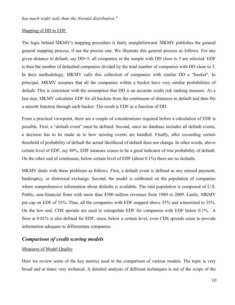
Mapping of DD to EDF

The logic behind MKMV's mapping procedure is fairly straightforward. MKMV publishes the general

general mapping process, if not the precise one. We illustrate this general process as follows. For any

given distance to default, say DD=5, all companies in the sample with DD close to 5 are selected. EDF

is then the number of defaulted companies divided by the total number of companies with DD close to 5.

In their methodology, MKMV calls this collection of companies with similar DD a "bucket". In

principal, MKMV assumes that all the companies within a bucket have very similar probabilities of

default. This is consistent with the assumption that DD is an accurate credit risk ranking measure. As a

last step, MKMV calculates EDF for all buckets from the continuum of distances to default and then fits

a smooth function through each bucket. The result is EDF as a function of DD.

From a practical viewpoint, there are a couple of considerations required before a calculation of EDF is

possible. First, a “default event” must be defined. Second, since no database includes all default events,

a decision has to be made as to how missing events are handled. Finally, after exceeding certain

threshold of probability of default the actual likelihood of default does not change. In other words, above

certain level of EDF, say 40%, EDF measure ceases to be a good indicator of true probability of default.

On the other end of continuum, below certain level of EDF (about 0.1%) there are no defaults.

MKMV deals with these problems as follows. First, a default event is defined as any missed payment,

bankruptcy, or distressed exchange. Second, the model is calibrated on the population of companies

where comprehensive information about defaults is available. The said population is composed of U.S.

Public, non-financial firms with more than $300 million revenues from 1980 to 2009. Lastly, MKMV

put cap on EDF of 35%. Thus, all the companies with EDF mapped above 35% and winsorized to 35%.

On the low end, CDS spreads are used to extrapolate EDF for companies with EDF below 0.1%. A

floor at 0.01% is also defined for EDF, since, below a certain level, even CDS spreads cease to provide

information adequate to differentiate companies.

Comparison of credit scoring models

Measures of Model Quality

Here we review some of the key metrics used in the comparison of various models. The topic is very

broad and at times very technical. A detailed analysis of different techniques is out of the scope of the

10

paper. Therefore, we focus on the methods used in our study and those closely related. For more detailed

analysis and bigger variety of tests, we refer the readers to other sources, which we list at the end of the

section.

As the finance community and the government regulatory bodies become more interested in measuring

credit risk, they develop new ways of evaluating and comparing credit models. For the models focusing

on the prediction of probability of default, validation proceeds along two different dimensions: model

discriminatory power and model calibration.

The power of a model refers to its ability to distinguish between defaulting ("low quality") and non-

defaulting ("high quality") firms. For example, if two models produce two ratings, "high quality" and

"low quality," the more powerful model would have a higher percentage of defaults and a lower

percentage of non-defaults in its "low quality" category and had a higher percentage of non-defaults and

a lower percentage of defaults in its "high quality" category. This type of analysis can be performed

using power curves, for example.

Calibration describes how well a model's predicted probabilities match with observed events. For

example, assume we have two models, A and B, each predicting two rating classes, "high quality" and

"low quality". If the predicted probability of default for A's "low quality" class are 5% B's is 20%, we

might examine these probabilities to determine how well they matched actual default rates. If we looked

at the actual default rates of the portfolios and found that 20% of B's "low quality" rated loans defaulted

while 1% of A's did, B would have the more accurate probabilities since its predicted default rate of

20% closely matches the observed default rate of 20%, while A's predicted default rate of 5% was very

different than the observed rate of 1%. This type of analysis can be performed using likelihood

measures.

Some of the most common methods for evaluating the discriminatory power of a credit scoring systems

include: Cumulative Accuracy Profile (CAP) and its Accuracy Ratio (AR), Receiver Operating

Characteristic (ROC) and Area under ROC curve (AUROC).

CAP and ROC are graphical presentations of the model’s discriminatory power. Although the graphs

themselves do not provide formal tests of model quality, they enable quick assessment of various

properties and may indicate which formal tests should be applied. They can also be seen as a credit risk

model version of the quantile-quantile plots used for evaluating distributions.

11

Engelmann et al. (2003) show that the AUROC and AR are simply linear transformations of each other.

Thus, having one of these statistics suffices, since no additional information can be extracted from the

other. The proof of the equivalence of AUROC and AR, and additionally the discussion on how to

statistically evaluate the difference between the ROC curves of two different models can be found in

Engelmann’s paper.

Evaluation of calibration of credit risk models poses additional challenges. A small number of default

events often makes it difficult or impossible to evaluate the relationship between true default frequency

and assigned probabilities of default for different risk classes within the same model. Therefore, the

measurement is often concentrated on comparing true default frequency for the whole sample with the

assigned probabilities of default. An alternative approach is to attempt to fit a regression model to the

data with credit scores, or forecasted default probabilities, as the explaining variable and default

(non-)events as the explained variable. A model with higher likelihood measure is considered to have

better calibration.

As mentioned at the beginning of this section, the topic of model evaluation and comparison techniques

is very broad and there is more specialized literature that covers it. For a general overview of the area we

direct the reader to Moody’s publications: Stein (2002) and Sobehart and Stein (2004). Engelmann et al.

(2003) provide an excellent overview of power curves evaluation techniques and their comparisons.

Tasche (2006) gives an overview of great variety of tests including: Spiegelhalter test, information

entropy, binomial test, Hosmer-Lemeshow test just to name a few. For more commercial publications on

the topic refer to Christodoulakis and Satchell (2008) and, especially for Basel II relevant methodology,

Ozdemir and Miu (2009).

Empirical Evidence from Model Comparison

This section provides an overview of the empirical studies comparing various credit scoring models.

Though there are a substantial number of models, there is a relative scarcity of studies that rigorously

evaluate the contribution of different approaches. One problem with empirical tests of models’ quality is

difficulty with obtaining large datasets. Since corporate defaults are fairly rare events only very

comprehensive databases might contain all the information required to conduct the tests. Other

important fact is that the development of some of the more rigorous statistical tests occurred rather

recently. The movement was spurred in a big part by the new Basel capital accord.

We begin by reviewing the results of a survey study that takes a bit different angle on the measurement

12

of the credit risk model quality. The study evaluates ability to valuate risky debt with contingent-claims

credit models – Bohn (2000). Next, we present an important study by Shumway (2001). We also

mention Duffie et al. (2007), which suggests an interesting credit risk model, though difficult to compare

with MKMV. We then focus on studies that evaluate contingent-claim credit risk models similar in form

to MKMV. Papers discussed include Hillegeist et al. (2004), Bharath and Shumway (2008), Agarwal

and Taffler (2008). Finally, we give a quick overview of a study - Sobehart and Stein (2004), as

presented by the researchers employed by MKMV.

A survey by Bohn (2000) reveals an abundance of structural and reduced-form models for use in credit

risk and risky debt valuation. Bohn explains that, despite this variety of models, there is a relative

scarcity of empirical tests on bond data. In practice, the amount and quality of corporate bond data is

very limited. This, coupled with the relative complexity of bond structures and the large number of

parameters required for structural models, make empirical testing very challenging. Consequently,

studies that attempt to perform the tests often focus on special cases or limited samples. In this setting, it

is unrealistic to expect generalizable and statistically robust results.

Bohn's review indicates weak-to-mixed support for the contingent-claim models’ ability to explain bond

spreads. Early papers from Jones, Mason, and Rosenfeld (1984) and Franks and Torous (1989) find a

significant mismatch between structural model spread predictions and true spreads. Another paper from

the same year, Sarig and Warga (1989), report that the predicted term structures of credit spreads are

consistent with the observed term structures. However, a small sample and lack of rigorous statistical

testing prevented them from drawing strong conclusions. Another paper with small sample that finds

support for Merton framework is Wei and Guo (1997). Delianedis and Geske (1998) use the Black-

Scholes-Merton framework to estimate risk-neutral default probabilities and test them on rating

migration and default data. They find evidence that the bond market predicts default events faster than

the equity market.

Overall, it seems that the research in this area is still open. Even though the contingent-claim models

have solid theoretical foundation there is no strong evidence that they can predict bond spreads.

In his paper, Shumway (2001) develops a hazard model and then tests its discriminatory power against

accounting-based z-score model. Another important finding, the paper determines that a discrete time

logit model can be estimated as a simple logit model with correction for the multiple years per firm. We

apply this approach in our study.

13

Shumway estimates his model and tests it on 31 years of bankruptcy data. He finds that the model

outperforms the accounting-based model. He also reports that, by combining certain market variables

and accounting information, one can significantly improve the predictive power of a model.

As mentioned, many of rigorous tests for the credit risk model quality were developed fairly recently,

and thus, absent from Shumway’s study. A comparison of the discriminatory power is limited to the

forecast accuracy tables, which might be described as crude form of Cumulative Accuracy Profiles

(CAP). Furthermore, we notice that some comparisons are performed on different samples for two

different models. This undermines the quality of the comparison, as the sensitivity of CAP to changes in

the underlying sample is high. Although Shumway contributes by developing the hazard model and

showing the properties of discrete time logit estimation, we find his evaluation of the model quality

insufficient.

Duffie et al. (2007) provide maximum likelihood estimators of term structures of conditional

probabilities of corporate default, incorporating the dynamics of firm-specific and macroeconomic

covariates. Their out-of-sample forecasts produce remarkable results that seem to dwarf other common

credit risk models. Although their results look impressive, it is impossible to reliably compare the

discriminatory power of their model and MKMV’s since they were not tested on the same samples.

Hillegeist et al. (2004) assess whether two popular accounting-based measures, Altman’s (1968) Z-score

and Ohlson’s (1980) O-score effectively summarize publicly available information about the

probabilities of default. They compare the relative information content of these scores with the

probabilities of default derived from Black-Scholes-Merton model.

They find that, irrespective of various modifications in the accounting-based credit models, the

contingent-claim model always outperforms the Z-score and O-score. The test for the information

content is of the same form as the one applied in our study. We also use their method to transform our

probabilities of default in the into logit scores. Though their contingent-claim model relies on the

normal distribution to derive the implied probabilities of default, the results indicate superior

performance of this market-based model.

Bharath and Shumway (2008) investigate a credit risk model that mimics MKMV expected default

frequency against a simpler alternative that takes similar functional form and compare their default

prediction abilities. They also investigate the correlation of the implied probabilities of default with

credit default swaps and corporate bond yield spreads. They find that their naïve version of MKMV

14

performs at least as well as the MKMV predictions. They also report that solving iteratively for the

value of assets, as described in MKMV methodology, is less important and that solving simultaneously

for asset value and volatility yields a model with higher predictive power. Finally, the correlation

between MKMV model predictions and the observed CDS and bond yield spreads are weak after

correcting for agency ratings, bond characteristics, and their alternative naïve predictor.

As we argue in the introduction, the model presented by Bharath and Shumway is not an appropriate

proxy for the true MKMV, since it assumes normal distribution of distances to default. Our further

criticism of their paper includes the evaluation method used to compare the models’ quality. Once again,

as in Shumway (2001), the sole reliance on accuracy tables to compare the discriminatory power of the

models seems insufficient.

Agarwal and Taffler (2008) present a comparison of contingent-claim and accounting-based credit risk

models in their ability to predict corporate defaults on the UK market. Apart from two tests that are

similar to those previously utilized in the literature, they also employ a simulation that helps to evaluate

the quality of the models when the misclassification error costs differ. For the purpose of our study, we

draw heavily from their methodology. It seems that their evaluation approach and the model comparison

methods are the most comprehensive among the papers reviewed. They allow for testing the models’

power (ROC) and calibration (through the information content test and the simulation).

The main findings of their paper are that there is little or no difference in the discriminatory power of

accounting-based Z-score and BSM prediction of probability of default; and very little difference in the

information content of the two models (they seem to have similar amount of information, but slightly

different sets of information). The notable difference between the two models is identified in the

simulation. Agarwal and Taffler show that slightly higher information content of the Z-score leads to

supreme performance of a bank that applies this method.

Finally, we look at the results presented by Soberhart and Stein (2004) who evaluate the actual MKMV

model against other popular credit risk models. Although their paper focuses on the model validation

methodology, they present some results of the comparison too. According to their CAP results and

accuracy ratios, the actual MKMV model outperforms a simple Merton model, Z-score and a tested

version of hazard model.

Though the last paper includes the results of tests where the actual MKMV is evaluated against other

methods, other references rely on cumulative normal distribution as a mapping function from distance to

15

default (DD) to probability of default (PD) when referring to contingent-claim approaches.

Results are mixed as to whether the contingent-claim approach to credit risk evaluation is superior to

other methods, but we also see a problem of incoherence. It seems that researchers have been applying

normal distribution to calculate the implied probabilities of default from the BSM models. Unlike the

research community, the actual MKMV model uses empirical default frequency to map DD to PD.

Therefore, it seems questionable whether we can infer the properties of true MKMV model from the

theoretical models presented in the literature. Our study aims at confronting the two models and

evaluating whether we can bridge the gap between the models or should we rather re-evaluate the

quality of MKMV default predictions.

16

Part 3 – Data and MethodologyWe give an overview of the data used in our approach. A presentation of the methodology used follows.

Data

In order to process the EDF approach to the KMV model, we gathered the type of data likely found in

the MKMV database, such as default events and other company-specific data. A SQL-Server 2008

database was constructed and populated for this purpose.

We gathered a list of about 221 default events by month and year from Moody’s Default Research

comments7. Defaults included corporate bond, commercial paper, and syndicated loan defaults for

publicly traded firms spanning the 15 years between 1993 and 2008. We supplement this with financial

statements, stock prices, volatilities, pulled from DATASTREAM. This data was gathered for all

defaulted companies and an additional 2,914 going concerns, for a total of 3,254 companies. See Table 1

for a summary of company year data and default information by year and time horizon. The shaded area

indicates that data was not used in the study due insufficient information. Company information was

gathered over the 15 years 1992- 2007 when available, giving a total sample of 33,350 company years.

US Treasury Bill rates were also pulled from DATASTREAM for each of the above years for use as

risk-free rate in Distance to Default calculations. The lagged sample default frequencies were used in the

logistic regressions as a proxy for baseline hazard rates for the corresponding time horizons.

7 Http://www.moodys.com

17

It is important to note that our sample default frequencies are very close to half the default rates reported

by Moody’s. The reason for our population of defaulters being smaller than Moody’s is that for some

defaulters we weren’t able to obtain all the information required for the tests. Therefore, the defaulters

with missing data were dropped from the sample.

In the following methodology section, we define a company's “company year” data as the market price

and volatility as of September 30th in a given year, with long and short term debt obtained from the last

available annual report. A September market date is chosen, per the example of Agarwal and Taffler

(2008), to ensure that all the information was available at the time of portfolio formation. Consequently,

we also maintain this data within our definition of the default events used in our calculation of empirical

EDF, and later, testing of respective model strengths. In each case, a default event is declared for a

company year if default occurred within the specified time horizon as measured from September 30 th of

the company year. 1yr, 2yr, 3yr, and 5yr US Treasury Bill rates were also pulled as of this date,

respective for each time horizon modeled. We use the average of 3 and 5 -yr rates to model Distance to

Default for 4 year time horizons.

It should be noted that this sample size is significantly smaller than that of that used in the actual

MKMV database. Since the quality of an EDF is strongly related to the quantity of underlying data

available to it, one would reasonably expect the EDF of Moody's KMV model to provide a greater

predictive power.

18

Table 1Year Number of default events w ithin Sample default frequency w ithin

1 year 2 years 3 years 4 years 5 years 1 year 2 years 3 years 4 years 5 years1992 2,127 5 8 10 13 19 0.24% 0.38% 0.47% 0.61% 0.89%1993 2,130 3 5 8 14 24 0.14% 0.23% 0.38% 0.66% 1.13%1994 2,081 2 5 11 24 34 0.10% 0.24% 0.53% 1.15% 1.63%1995 2,388 3 10 25 41 67 0.13% 0.42% 1.05% 1.72% 2.81%1996 2,418 7 24 43 74 99 0.29% 0.99% 1.78% 3.06% 4.09%1997 2,342 11 34 68 94 121 0.47% 1.45% 2.90% 4.01% 5.17%1998 2,216 27 60 91 118 132 1.22% 2.71% 4.11% 5.32% 5.96%1999 2,337 29 66 98 114 125 1.24% 2.82% 4.19% 4.88% 5.35%2000 2,155 35 71 88 99 107 1.62% 3.29% 4.08% 4.59% 4.97%2001 2,022 37 57 68 79 84 1.83% 2.82% 3.36% 3.91% 4.15%2002 1,920 17 28 38 44 53 0.89% 1.46% 1.98% 2.29% 2.76%2003 1,815 10 21 27 35 49 0.55% 1.16% 1.49% 1.93% 2.70%2004 1,701 8 15 20 34 40 0.47% 0.88% 1.18% 2.00% 2.35%2005 1,580 5 10 26 33 33 0.32% 0.63% 1.65% 2.09% 2.09%2006 1,486 6 22 31 31 31 0.40% 1.48% 2.09% 2.09% 2.09%2007 1,374 11 20 20 20 20 0.80% 1.46% 1.46% 1.46% 1.46%2008 1,258 5 5 5 5 5 0.40% 0.40% 0.40% 0.40% 0.40%

Sum : 33,350 221 461 677 872 1043 0.65% 1.34% 1.95% 2.48% 2.94% : Avg

Observations count

Model Methodology

Calculating Distance to Default

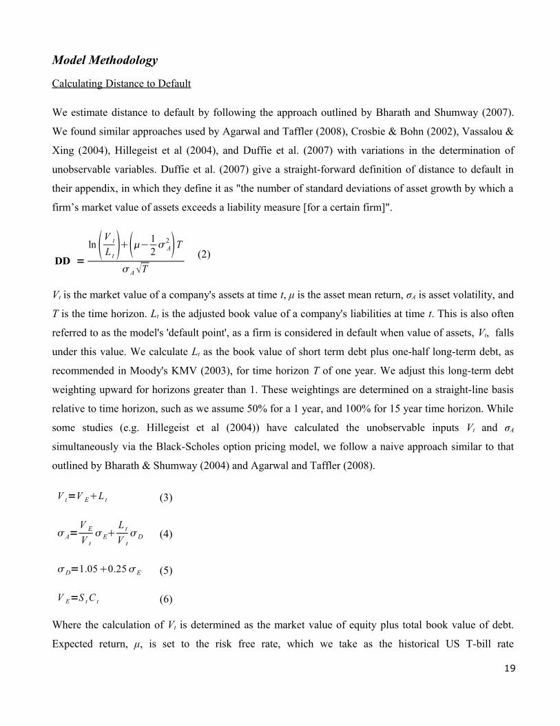
We estimate distance to default by following the approach outlined by Bharath and Shumway (2007).

We found similar approaches used by Agarwal and Taffler (2008), Crosbie & Bohn (2002), Vassalou &

Xing (2004), Hillegeist et al (2004), and Duffie et al. (2007) with variations in the determination of

unobservable variables. Duffie et al. (2007) give a straight-forward definition of distance to default in

their appendix, in which they define it as "the number of standard deviations of asset growth by which a

firm’s market value of assets exceeds a liability measure [for a certain firm]".

DD =ln V t

L t −12 A

2 T

AT(2)

Vt is the market value of a company's assets at time t, μ is the asset mean return, σA is asset volatility, and

T is the time horizon. Lt is the adjusted book value of a company's liabilities at time t. This is also often

referred to as the model's 'default point', as a firm is considered in default when value of assets, Vt, falls

under this value. We calculate Lt as the book value of short term debt plus one-half long-term debt, as

recommended in Moody's KMV (2003), for time horizon T of one year. We adjust this long-term debt

weighting upward for horizons greater than 1. These weightings are determined on a straight-line basis

relative to time horizon, such as we assume 50% for a 1 year, and 100% for 15 year time horizon. While

some studies (e.g. Hillegeist et al (2004)) have calculated the unobservable inputs Vt and σA

simultaneously via the Black-Scholes option pricing model, we follow a naive approach similar to that

outlined by Bharath & Shumway (2004) and Agarwal and Taffler (2008).

V t=V EL t (3)

A=V E

V tE

L t

V tD (4)

D=1.050.25E (5)

V E=S t C t (6)

Where the calculation of Vt is determined as the market value of equity plus total book value of debt.

Expected return, μ, is set to the risk free rate, which we take as the historical US T-bill rate

19

corresponding to the appropriate time horizon T, as outlined previously in the Data section. σE is simply

the standard deviation of stock returns calculated over the past year. Value of equity, VE, is a given

company's market capitalization, which we calculate as the market share price St multiplied by the

number of shares outstanding Ct.

We calculate Distance to Default thus for every company year represented in our sample for each time

horizon tested – specifically, T of one, two, three, four, and five years.

Mapping DD to Probability of Default assuming Normal Distribution

The first of two approaches we use to estimate probability of default simply relies on the cumulative

normal distribution as a function to transform our previously calculated distance to default (DD) to

probability. In doing so, we follow the most commonly tested approach (see Equation 2 for definitions):

P def = (-DD) = N ln V A,t

X t −12 A

2T AT (7)

The resulting value is interpreted as the probability, between 0 and 1, that a given firm will default

within the stated time horizon and is calculated for all DDs.

Mapping DD to EDF

In our second approach, we attempt to simulate MKMV’s EDF mapping procedure. Thus, we abandon

the assumption of normal distribution in an effort to capture a closer representation of probability of

default distribution from our combined samples of company year data and actual historical default

events.

We accomplish this by first sorting company year data in ascending order of calculated DD for a given

time horizon. This data is then organized into overlapping groups, or 'buckets', of 1,075 company years

each (for a 1 year horizon). Each bucket's median DD is identified as the bucket's representative DD

value. The Expected Default Frequency (EDF) for the bucket is identified as the sum of all historical

defaults within the bucket divided by bucket size (1,075). The result is essentially a historical default

rate associated with a specific DD value (the bucket's median). This process is then repeated, with the

bucket shifting one record at a time, through all sorted DDs to the end of the sample. This is done

separately for each time horizon. The resulting list of DD values and associated default rates by time 20

horizon is used as the distribution in our next step, in which we calculate default probabilities.

On a side note, a bucket size of 1,075 was determined as optimal based on a comparative analysis of

forecasting strength as determined from a wide range of tested buckets sizes. Please see 'Estimation of

Optimal Bucket Size' in the appendix for more information on this process.

Of course, by the nature of the process, some DDs and default rates at the lower and upper extremes are

necessarily excluded from the above results. The number excluded is approximately equal to the bucket

sized used; half at the lowest, and half at the highest, extremes will fail to appear as a representative

median of any bucket.

It should also be noted that the above is a simplification of the process, as some modifications are

required to provide a logically coherent basis for later comparison of historical forecast abilities

between the two models. In our first approach, the normal distribution that defines the mapping between

DD to probability of default does not change over time, since additional information gained does not

change the nature of normal distribution itself. On the other hand, determination of EDF must logically

be limited to information available at the time a forecast is made. Thus, the above approach is repeated

for each year we attempt to forecast (1993-2008), with company years occurring after the forecast date

excluded from EDF calculations. Intuitively, the accuracy of EDF distributions can be expected to

improve in later forecast dates as additional sample data becomes available.

In a similar line of thought, the nature and use of time horizons in the determination of an event

occurring further limits potential EDF calculations made for a given sample. For example, when

calculating 3-year horizon EDF forecast for the year 2000, one cannot include 3-year horizon DD and

default events from 1999 in the calculation, since the referenced default events had not yet occurred.

Thus, given a finite data set, one can imagine the list of all possible forecast year (y-axis) and time

horizon (x-axis) combinations as rightward pointing triangle meeting at a point beyond which no higher

time horizon can be calculated for any forecasted year. Thus, one would intuitively expect EDF

distribution accuracy to decrease in quality as time horizon increases and potential sample size

decreases.

We illustrate the process with an example of determination of a single DD to EDF mapping. We sort the

list of all DDs and default events. If we are forecasting for the year 2007 and a 3-year time horizon, we

exclude from the list all DDs calculated for time horizons other than 3 years. We also exclude from this

21

sorted list all DD's calculated on company years after 2007. Also removed are all DD's with default

events occurring after 2007. For a time horizon of 3 years, this would be all DDs calculated after 2007

minus three years, or all such DD's calculated after 2004. With available default data starting in 1993,

we are first able to calculate DD with default events in 1993 plus 3 years, or 1996. Years previous to this

are also not included in the list. With our list of DDs and default events defined and sorted in this way,

we define our first bucket as all DDs between the lowest and 1,075th lowest DD. We take the median DD

in this bucket as the bucket's defining DD. We then sum of all corresponding default events occurring

within three years. We divide this sum by 1,075 to determine the EDF for the bucket's median DD. This

process is repeated for the next bucket, defined as the DD's between the 2nd lowest and 1,076th lowest

DD, and so on, repeated for all feasible years time horizon combinations. This gives us a EDF

distribution table by forecast year and time horizon associating each bucket's median DD with an EDF.

Finally, the probability of default is calculated for each company year and DD using the distribution

table just described. The distribution table is referenced for the time horizon, company year, and DD to

be forecasted. The closest DD is identified in EDF distribution table, and that EDF is accepted as the

probability of default for the DD in question. This process is repeated for all company DDs and time

horizons. As with the normal distribution approach, the resulting values are interpreted as the

probability, between 0 and 1, that a given firm will default within the stated time horizon.

Model Evaluation Methodology

In the following three tests, we roughly follow the evaluation approaches outlined by Agarwal, Taffler

(2008). As suggested by Sobehart et al (2004), we conduct walk-forward testing to ensure out-of-

sample, out-of-time and out-of-universe test. In short, we estimate the models on all the data available

up to year t. Then we use the models to forecast the PD for the next year for all the companies that

existed in the sample before year t (conditional on their survival until year t) and all the companies that

have just entered the sample in year t. We save the pairs of data-points – (forecasted PD, default event=1

or no event=0 in year t+1) for all the companies. We then add year t+1 to our in-sample, re-estimate the

models, and repeat the procedure as before.

The three tests described below measure model power, or predictive ability; unique information content;

and practical economic value, respectively.

22

Methodology - Testing Predictive Ability - The ROC curve

Receiver operating characteristics, or ROC curve, plots the sensitivity for a binary classifier system and

can be used to measure and compare the predictive ability of various models. Since it was first

developed by radar engineers in World War II as a tool to improve aircraft detection, ROC curves have

been used to assess model quality across a wide range of disciplines including psychology, finance, and

medicine. When applied to internal credit rating models, Sobehart and Keenan (2001) find area under

the ROC curve is indicative of model quality.

The ROC curve categorizes model results into two simple categories – correct, or not correct. Thus, it

does not distinguish between type I and type II errors. In practice, the two errors have very different

impacts. In the case of a type I failure, in which the model wrongly predicts a future defaulter will not

fail, the entire amount lent may be lost. With a type II error, we wrongly predict that a future non-

defaulter will default, which simply implies a lending opportunity lost.

With this caveat in mind, the ROC curve is a graph depicting the power of a model. It is a plot of the

false alarm rate (x axes) against the hit rate (y axes) for all possible cut-off points from the range of

default probabilities. The area under ROC curve (AUROC) is the Wilcoxian (or equivalently, Mann-

Whitney) statistic. We test the difference between the AUROCs as described by Engelmann et al (2003),

using the online StAR ROC Analysis Tool provided by the Molecular Bioinformatics Laboratory at the

Pontificia Universidad Católica de Chile8. Into this, we input the NPD and EDF probabilities with

corresponding default events for 1-5 year time horizons.

Methodology - Testing Information Content – Hazard Model

Hillegeist et al. (2004) note that, in the lending business, it is common to accept the majority of

borrowers, then differentiate pricing depending on their credit quality. Thus, the decision is not simply

whether a loan should be granted or not, but rather how a loan should be priced. If this is the case, the

tests for model discriminatory power, like ROC curve, do not provide a full picture. Hillegeist et al.

(2004) suggest a test for the information content of a credit scoring model. The test is performed by

fitting a discrete time logit model to the data. A model that better fits/explains the data is considered to

bare more information content. It takes the following form:

8 http://protein.bio.puc.cl/cardex/servers/roc/roc_analysis.php

23

P i,t=e t X i , t

1e t X i , t (8)

Where Pi,t is probability of default of firm i at time t in the next 12 months for one-year horizon, 24

months for 2-year horizon, etc. α(t) is baseline hazard rate proxied by the trailing year failure rate in our

sample, X is matrix of independent variables and β is a column vector of estimated coefficients.

Shumway (2001) shows that the model can be estimated as a simple logit regression. However, this

introduces an inherent bias into the standard errors, as there are multiple observations for the same

company in the sample. He suggests adjusting the test statistic by dividing it by the average number of

observations per firm to obtain unbiased standard errors.

Similar to Hillegeist et al. (2004) and Agarwal, Taffler (2008), our credit risk models return probability

of default as output. These probabilities cannot be used directly in the logistic regressions, as this would

violate the underlying assumptions of logit model. Therefore, as suggested in the two papers, we

transform the probabilities of default from our models into logit scores by:

score=ln p1− p (9)

Following the convention from the two papers, we winsorize the probabilities to a narrower range to

avoid arbitrarily small (or large) scores. Thus, we set all the probabilities of default from our two models

to 0.00000001 if they are lower than this value, or 0.99999999 if higher. Thus, the scores are within the

range +/-18.4207.

Finally, we compare the fit of the models to the data by performing a Clarke test. Though a Vuong test

for the difference in mean log-likelihood is often performed in this situation, we drop this evaluation

method for two reasons: (1) the test is less powerful for data with high kurtosis (the kurtosis of our log-

likelihoods ranges from 30 to 300), and (2) the initial estimations showed that the test is inconclusive for

all the possible tested pairs of models. The Clarke test is a non-parametric test for the difference in

median log-likelihood of two models. It performs particularly well when the data is very concentrated,

as it is in our case. A more detailed discussion, comparison with Vuong test and example of monte carlo

experiment are presented in Clarke (2003).

In short, the Clarke test is performed as follows. First we estimated the two models that we want to

compare, saving the individual log-likelihoods from the estimations. We then perform a paired sign test

24

for the difference in median log-likelihood. A paired sign test does not make any assumption about the

shape of the distribution in the two samples compared. If the median log-likelihoods of the two tested

models are different, then the two models bare different information content. We perform both one-sided

and two-sided tests to determine which model is better.

Methodology - Testing Economic Value – Lending Simulation

In our third and final test, we seek to capture the practical effectiveness of using the two models to drive

the lending decision. In practice, there is a significant difference between the cost of giving a loan to

poor quality borrower and cost of not giving loan to good quality borrower. We roughly follow the

informal approach outlined by Agarwal, Taffler (2008), by which we replicate a competitive setting of

two banks. In our simulation, one bank relies exclusively on the NPD model, the other on our EDF

approach. The simulated banks then compete for borrowers from our sample. At the end of the sample

period we evaluate their profitability (ROA), risk-adjusted profitability (RORWA), and other measures.

Agarwal, Taffler (2008) argue that this simulation is a test for the effect of model power on the

profitability of banks that apply it. In our case, the test is also a calibration measure. Since the ranking of

the borrowers provided by the two evaluated models is virtually identical, the hazard model used in the

calculation of the loan spreads will effectively calibrate the two models.

We utilize Excel VBA to run our simulation in all years that EDF forecasts are possible for a given time

horizon. For a one year horizon, this turns out to be 1994 through 2007. We repeat the process for a two

year (1995-2006), three year (1996-2005), four year (1997-2004), and five year (1998-2003) horizons.

This conforms to industry reality, as banks can be assumed to recalibrate their forecasts of default

probabilities every year. For us, it means that every year we must re-estimate a logit regression of the

same form as Equation 8. The out-of-sample forecasts of probabilities of default are used for calculating

the interest rate spread that the banks charge their clients. For the sake of simplicity, we assume that the

banks have complete prior-year information for all companies. Like Agarwal and Taffler (2008), we

follow Blochlinger and Leippold (2006a) in deriving the credit risk spread as the following function of

the probability of default:

R= p Y =1 | S=t p Y =0 | S=t

LG Dk (10)

Where R is the credit spread, p(Y=1|S=t) is conditional probability of failure for a score of t, p(Y=0|S=t)

is the conditional probability of non-failure for score t, LGD is loss given default, and k is the credit

25

spread for the highest credit quality loan.

In our simulation we follow the methodology outlined by Agarwal and Taffler (2008). We assume a loan

market worth $100 million and each loan of equal value. Both banks refuse loans to companies scoring

in the lowest 5th percentile as measured within their respective models. The hazard model, from the last

test, is used to calculate the credit spread quoted to all accepted companies. For the purpose of the

simulation, we assume that the credit spread for the highest quality customers, k, is equal to 0.30% for

both banks. The LGD of 45% is assumed to be constant and equal for both banks. Companies choose

the bank offering the best deal. If the spreads are identical, each bank simply receives 50% of the

business. We track bank market share, the loans granted each year, the share of defaulters each bank

receives, average spread, and nominal profit. To assess the economic value of each model, we use return

on assets (ROA) and the return on risk weighted assets (RORWA) as follows:

ROA= PROFITTOTAL VALUE OF LOANS GRANTED (11)

RORWA = PROFITTOTAL VALUE OF RISK WEIGHTED LOANS GRANTED (12)

Like Agarwal and Taffler (2008), we calculate BIS risk as per the Basel II Foundation Internal Ratings-

based Approach9. The risk-weight (RW) for each loan is determined using the following formulas:

RW =12.5∗K (13)

K =[LGD∗N { 11−R

G PD R1−R

G 0.999}−LGD∗PD]1M −2.5∗b PD1−1.5∗b PD

(14)

R= 0.121−e−50∗PD

1−e−500.24[1−1−e−50∗PD1−e−50 ] (15)

b=0.11852−0.05478∗ln PD 2 (16)

Where, G(.) is the inverse cumulative normal distribution, N(.) is cumulative normal distribution and M

is loan maturity.

9 Basel Committee on Banking Supervision (2006, pp. 63–64)

26

Part 4 – Empirical ResultsH0: There is no significant difference between KMV model based on normal distribution (here we refer

to naïve model suggested by Bharath and Shumway (2004)) and the empirical distribution of the KMV-

based model described earlier.

Model Results

Fig. 1a - PD for 1yr horizon Fig. 1b - PD for 5yr horizon

In Figures 1a and 1b we show the distributions EDF and NPD as a function of distance to default for

one-year (bucket size = 1,175) and five-year time horizons (bucket size = 300), respectively. One can

note that, while both functions decrease over the majority of their domain, EDF demonstrates multiple

peaks.

27

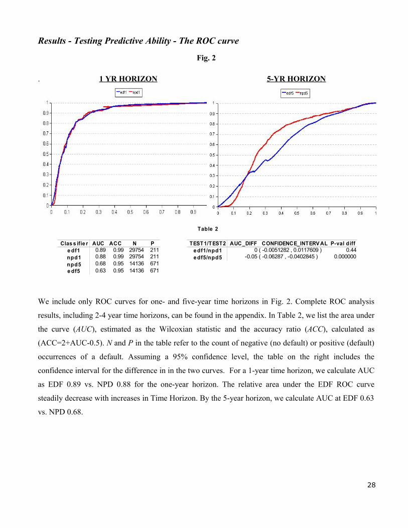
Results - Testing Predictive Ability - The ROC curve

Fig. 2

. 1 YR HORIZON 5-YR HORIZON

We include only ROC curves for one- and five-year time horizons in Fig. 2. Complete ROC analysis

results, including 2-4 year time horizons, can be found in the appendix. In Table 2, we list the area under

the curve (AUC), estimated as the Wilcoxian statistic and the accuracy ratio (ACC), calculated as

(ACC=2+AUC-0.5). N and P in the table refer to the count of negative (no default) or positive (default)

occurrences of a default. Assuming a 95% confidence level, the table on the right includes the

confidence interval for the difference in in the two curves. For a 1-year time horizon, we calculate AUC

as EDF 0.89 vs. NPD 0.88 for the one-year horizon. The relative area under the EDF ROC curve

steadily decrease with increases in Time Horizon. By the 5-year horizon, we calculate AUC at EDF 0.63

vs. NPD 0.68.

28

Table 2

Clas s ifie r AUC ACC N P TEST1/TEST2 AUC_DIFF CONFIDENCE_INTERV AL P-val diffe df1 0.89 0.99 29754 211 e df1/npd1 0 ( -0.0051282 , 0.0117609 ) 0.44npd1 0.88 0.99 29754 211 e df5/npd5 -0.05 ( -0.06287 , -0.0402845 ) 0.000000npd5 0.68 0.95 14136 671e df5 0.63 0.95 14136 671

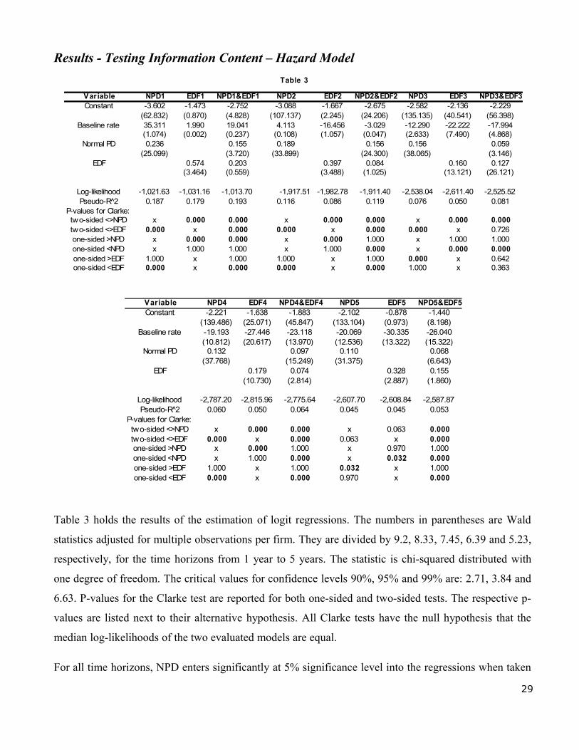
Results - Testing Information Content – Hazard Model

Table 3 holds the results of the estimation of logit regressions. The numbers in parentheses are Wald

statistics adjusted for multiple observations per firm. They are divided by 9.2, 8.33, 7.45, 6.39 and 5.23,

respectively, for the time horizons from 1 year to 5 years. The statistic is chi-squared distributed with

one degree of freedom. The critical values for confidence levels 90%, 95% and 99% are: 2.71, 3.84 and

6.63. P-values for the Clarke test are reported for both one-sided and two-sided tests. The respective p-

values are listed next to their alternative hypothesis. All Clarke tests have the null hypothesis that the

median log-likelihoods of the two evaluated models are equal.

For all time horizons, NPD enters significantly at 5% significance level into the regressions when taken

29

Variable NPD4 EDF4 NPD4&EDF4 NPD5 EDF5 NPD5&EDF5Constant -2.221 -1.638 -1.883 -2.102 -0.878 -1.440

(139.486) (25.071) (45.847) (133.104) (0.973) (8.198)Baseline rate -19.193 -27.446 -23.118 -20.069 -30.335 -26.040

(10.812) (20.617) (13.970) (12.536) (13.322) (15.322)Normal PD 0.132 0.097 0.110 0.068

(37.768) (15.249) (31.375) (6.643)EDF 0.179 0.074 0.328 0.155

(10.730) (2.814) (2.887) (1.860)

Log-likelihood -2,787.20 -2,815.96 -2,775.64 -2,607.70 -2,608.84 -2,587.87Pseudo-R̂ 2 0.060 0.050 0.064 0.045 0.045 0.053

P-values for Clarke:two-sided <>NPD x 0.000 0.000 x 0.063 0.000two-sided <>EDF 0.000 x 0.000 0.063 x 0.000one-sided >NPD x 0.000 1.000 x 0.970 1.000one-sided <NPD x 1.000 0.000 x 0.032 0.000one-sided >EDF 1.000 x 1.000 0.032 x 1.000one-sided <EDF 0.000 x 0.000 0.970 x 0.000

Table 3

Var iable NPD1 EDF1 NPD1&EDF1 NPD2 EDF2 NPD2&EDF2 NPD3 EDF3 NPD3&EDF3Constant -3.602 -1.473 -2.752 -3.088 -1.667 -2.675 -2.582 -2.136 -2.229

(62.832) (0.870) (4.828) (107.137) (2.245) (24.206) (135.135) (40.541) (56.398)Baseline rate 35.311 1.990 19.041 4.113 -16.456 -3.029 -12.290 -22.222 -17.994

(1.074) (0.002) (0.237) (0.108) (1.057) (0.047) (2.633) (7.490) (4.868)Normal PD 0.236 0.155 0.189 0.156 0.156 0.059

(25.099) (3.720) (33.899) (24.300) (38.065) (3.146)EDF 0.574 0.203 0.397 0.084 0.160 0.127

(3.464) (0.559) (3.488) (1.025) (13.121) (26.121)

Log-likelihood -1,021.63 -1,031.16 -1,013.70 -1,917.51 -1,982.78 -1,911.40 -2,538.04 -2,611.40 -2,525.52Pseudo-R̂ 2 0.187 0.179 0.193 0.116 0.086 0.119 0.076 0.050 0.081

P-values for Clarke:two-sided <>NPD x 0.000 0.000 x 0.000 0.000 x 0.000 0.000two-sided <>EDF 0.000 x 0.000 0.000 x 0.000 0.000 x 0.726one-sided >NPD x 0.000 0.000 x 0.000 1.000 x 1.000 1.000one-sided <NPD x 1.000 1.000 x 1.000 0.000 x 0.000 0.000one-sided >EDF 1.000 x 1.000 1.000 x 1.000 0.000 x 0.642one-sided <EDF 0.000 x 0.000 0.000 x 0.000 1.000 x 0.363

individually. EDF is also always significant in that case, but sometimes only at a 10% level. In

regressions where both credit scores were used as the explaining variables, we find that none of the

variables are significant on a 5% level for a 1 year horizon. The transformed credit scores for EDF range

from -18.42 to -2.59, while the range for NPD scores is +/-18.42.

Results - Testing Economic Value - Lending Simulation

We only include simulation results for one- and five-year time horizons in the the above results.

Complete simulation results, including the remaining 2-4 year time horizons, can be found in the

appendix.

For a one-year horizon, the return on risk-weighted assets for bank EDF increases almost tenfold

between 1994 and 2007, market share increases by about 20%, and share of defaulters drops by around

85%. In the meantime, bank NPD loses 20% market share and almost doubles it's share of defaulters.

One can also note that, for a five-year horizon, Bank EDF ROA and RORWA is consistently negative

while bank NPD's remains positive after the first year.

30

Ta ble 4

EDF – 1 yr Horizon NPD – 1 yr Horizon

YR Profit ROA RORW A P rofit ROA RORW A

1994 14,384 51.67% 60.58% 0.54% $76,380 0.15% 0.67% 12,532 45.02% 27.88% 0.51% $135,452 0.30% 1.36%1995 13,458 52.26% 60.68% 0.57% $79,088 0.15% 0.62% 11,438 44.41% 27.18% 0.54% $141,716 0.32% 1.30%1996 13,407 57.38% 61.58% 0.57% $85,874 0.15% 0.61% 9,177 39.27% 26.11% 0.59% $128,214 0.33% 1.33%1997 12,549 59.90% 62.24% 0.60% $97,987 0.16% 0.61% 7,702 36.76% 25.51% 0.66% $134,398 0.37% 1.35%1998 10,691 57.46% 61.62% 0.65% $96,299 0.17% 0.55% 7,309 39.28% 25.41% 0.67% $150,189 0.38% 1.26%1999 9,188 56.06% 63.29% 0.69% $112,172 0.20% 0.62% 6,667 40.67% 27.22% 0.69% $164,339 0.40% 1.24%2000 7,280 51.80% 57.36% 0.71% $129,999 0.25% 0.84% 6,287 44.73% 31.01% 0.67% $170,932 0.38% 1.28%2001 6,506 54.68% 57.45% 0.67% $161,195 0.29% 1.13% 4,949 41.59% 28.72% 0.68% $180,489 0.43% 1.66%2002 5,349 54.16% 38.60% 0.54% $191,741 0.35% 2.02% 4,120 41.71% 38.60% 0.63% $162,704 0.39% 2.23%2003 4,215 52.97% 20.00% 0.35% $141,594 0.27% 4.30% 3,381 42.49% 50.00% 0.58% $133,707 0.31% 5.06%2004 3,339 54.37% 13.33% 0.32% $144,387 0.27% 7.51% 2,495 40.63% 43.33% 0.51% $110,591 0.27% 7.70%2005 2,492 56.11% 13.64% 0.32% $149,256 0.27% 7.26% 1,727 38.89% 40.91% 0.47% $92,522 0.24% 6.50%2006 1,653 57.80% 5.88% 0.32% $168,523 0.29% 8.66% 1,066 37.27% 52.94% 0.46% $31,672 0.08% 2.52%2007 832 60.52% 9.09% 0.33% $164,069 0.27% 6.79% 475 34.53% 54.55% 0.46% -$36,474 -0.11% -2.65%

EDF – 5 yr Horizon NPD – 5 yr Horizon

YR Profit ROA RORW A P rofit ROA RORW A

1998 8,370 67.15% 87.45% 0.89% -$1,141,993 -1.70% -2.34% 3,922 31.46% 11.82% 0.67% -$22,687 -0.07% -0.10%1999 6,726 65.62% 88.76% 0.99% -$977,847 -1.49% -1.83% 3,423 33.39% 11.48% 0.72% $29,917 0.09% 0.11%2000 5,034 63.62% 89.42% 0.97% -$872,012 -1.37% -1.70% 2,800 35.38% 10.92% 0.71% $67,475 0.19% 0.24%2001 3,608 62.66% 89.78% 0.82% -$793,963 -1.27% -1.72% 2,089 36.28% 10.75% 0.60% $62,325 0.17% 0.23%2002 2,305 61.70% 90.20% 0.68% -$686,326 -1.11% -1.70% 1,384 37.04% 10.78% 0.53% $62,002 0.17% 0.26%2003 1,125 61.96% 89.80% 0.57% -$735,051 -1.19% -2.12% 666 36.67% 12.24% 0.45% $17,342 0.05% 0.08%

Loa ns Gra nte d

M kt S ha re

De fa ult Sha re

Avg S pre a d

Loa ns Gra nte d

Mkt Sha re

De fa ult Sha re

Avg Spre a d

Loa ns Gra nte d

M kt S ha re

De fa ult Sha re

Avg S pre a d

Loa ns Gra nte d

Mkt Sha re

De fa ult Sha re

Avg Spre a d

Part 5 – AnalysisModel Results

In Figures 1a/b we saw EDF and NPD distributions as a function of distance to default for one and five

-year time horizons. As to be expected with a limited number of annual observations, the EDF

distribution in Figure 1b is not a smooth, monotonically decreasing function. However, the resulting

function does decrease reasonably in the majority of its domain and is not dissimilar to the normal

distribution in overall form. While the graphs each show a peak in EDF, we apply that peak probability

value to all lower distance to defaults in actual results. Outside of this, no other smoothing is attempted.

We also note some sub-peaks in the EDF distribution. This implies, rather counter-intuitively, that

probability of default can increase (decrease) as the distance to default increases (decreases) over certain

small ranges. One desirable property of EDF is it's thicker tails compared to NPD. This can be clearly

seen in Figure 1b, but also in Figure 1a for DD range between 4 and 7. Finally, we see the five year

horizon distribution is more sporadic. This is likely a result of a reduction in the available sample set and

the smaller bucket sized required.

Overall, the shape of the EDF distribution appears to reasonably reflect the expected trend of lower DD

being associated with higher PD, particularly for the one-year horizon. Satisfied by this, we continue to

assess and compare the model to the NPD approach.

Results - Testing Predictive Ability - The ROC curve

The ROC curves in Fig. 2 yield some interesting information. Given a 1 year time horizon, we find that

the NPD and EDF approaches perform with similar power, with EDF usually at least as strong as NPD

in prediction ability, though not significantly. The relative area under the EDF ROC curve steadily

decrease with increases in Time Horizon. By the 5-year horizon, EDF strongly underperforms NPD over

the majority of it's domain (AUC 0.63 vs. NPD 0.68). We find that this decrease in EDF power is

consistent with the sample data loss, as noted earlier, associated with increases in time horizon. Rather,

we see this trait as speaking to the sensitivity of the EDF model to the size of the underlying available

sample, in general. Given this observed trend, we would anticipate continued positive movement of the

space under the EDF ROC curve as additional company and default samples are made available to the

model. Interestingly, EDF is consistently superior in its assessment of the lowest quality firms. This

quality could be useful in that (1) it allows banks to reject the absolute worst potential clients, and (2) it

31

allows banks to differentiate pricing based on the credit quality of lower quality firms.

It should be noted that the curves presented above are estimated for the whole sample; they average out

the early years when EDF was rather weak with relatively stronger recent years. Thus, if one were to

limit the graphed ROC curves to recent years, the space under the curve, and therefor power, of the EDF

model would increase relative to NPD. This would more likely be the case in practical use of the model,

as we are generally more concerned with future, rather than past, probabilities of default. We would, of

course, expect to observe the opposite effect when testing early years.

Results - Testing Information Content – Hazard Model

Before we can evaluate the results of the test in Table 3, it is important to note that the regressions were

estimated as of 30th September 2008, thus all the information about default events up to that point is

assumed to be known. There is no bias resulting from the use of information not available in the reality,

since our EDF estimates are always ex-ante. Normal probabilities of default are independent of time and

therefore there is no risk of introducing bias to the regression.

When we review the results of the regressions where both credit scores were used as the explaining

variables, we find that none of the variables are significant on a 5% level for a 1 year horizon. This is

despite the fact that the explaining power of the model is higher than for any individual scores. This

could mean that the scores bare very similar information.

These results seem intuitively consistent with those from the ROC analysis. However, it should be noted

that the models were estimated on the entire sample. This means that very early predictions of EDF

weight equally to the very recent ones. We are confident that their predictive powers are not the same,

and if so, the significance of the estimated coefficients is missing something. There is another important

factor that affects the results. The transformed credit scores for EDF range from -18.42 to -2.59, while

the range for NPD scores is +/-18.42. Consequently, EDF is far more sensitive to outliers than NPD. It

turns out that if we remove top 5 outliers (very few, in fact, for the sample of approximately 30,000

observations), the log-likelihood for EDF improves to the levels above log-likelihoods of NPD. We

don’t report these results, but mention them to offer context for the reader's interpretation of the

regression output.

The results from Clarke test provide strong evidence that the expected default frequency estimated from

the empirical sample contains more information about default events than that derived from distance to 32

default of a firm using normal distribution. In three out of five time horizons, the median log-likelihood

for EDF model is significantly higher than for the respective NPD model. These horizons are,

unsurprisingly, 1, and 2 and 4 years. For all the time horizons, the model that includes both scores

performs worse than the strongest individual models. This is as expected, as the credit scores bare

similar information, and the model with more coefficients is penalized by Clarke test for the lack of

parsimony.

To sum up, the test for the information content of the two credit scoring methods shows that they bare

similar information. Despite the first impression that EDF doesn’t offer any benefits, it turns out that

after closer examination for the shorter horizons, the empirical model outperforms the theoretical

distribution in terms of information content. Even if the two models have similar discriminatory power,

as could be interpreted from the ROC analysis, EDF calibrates better to fit the true default frequencies.

Results - Testing Economic Value - Lending Simulation

In Table 4, we saw the bank using EDF-based credit ratings show very strong performance in later years

relative to the bank using the NPD model for a one-year time horizon. With this horizon, Bank EDF is

better able to entice quality borrowers with lower spreads, thus gaining a larger market share over time,

while its share of the sample defaulters decreases. It seems that Bank EDF is better able than Bank NPD

to identify the best customers from the sample, while dismissing the worst. The behavior of the average

spread is indicative of the quality of an average bank customer. In general, as creditworthiness of the

average client increases, average spread decreases. We see this trend play out for Bank EDF. The

spreads for Bank NPD, on the other hand, seem to follow the credit cycle rather than a distinguishable

long-term trend. This may indicate that it captures customers in the mid-range of quality. Perhaps the

strongest measure of the economic value of the models, Bank EDF's ROA and RORWA consistently

improve over time, with a particularly dramatic increase seen in RORWA.

As we saw earlier, the quality of the EDF model increases with time, as the size of the underlying

available sample increases. We see both ROA and RORWA for Bank EDF surpass that of Bank NPD at

a certain point in time given a one-year horizon. Likely for similar reasons, Bank EDFs fortunes rapidly

turn for the worse as time horizon increases and sample availability decays. With a two-year time

horizon, we already see negative ROA for Bank EDF in all years, with Bank NPD remaining positive.

This trend continues to Bank EDFs abysmal results seen in the five-year time horizon results above.

Another interesting observation is that, for the longer horizons, Bank EDF wins mainly the poorest

33

quality customers. This relates directly to our observation from the ROC curves, where EDF seemed to

outperform NPD on the lower end of the credit quality.

With this final test, there is material evidence that EDF can outperform NPD, at least for the short time

horizons. The simulation also vividly demonstrates the change in the quality of EDF credit scoring as the

estimation samples increase. For a one-year horizon, the return on risk-weighted assets for bank EDF

increases almost tenfold between 1994 and 2007, market share increases by about 20%, and share of

defaulters drops by around 85%. These remarkable results should be compared with the 20% market

share loss and near doubling of share of defaulters experienced by bank NPD. Consistent with the results

from our previous test for information content, the bank utilizing EDF is better able to price loans for

prospective customers, thus winning market share from bank NPD and benefiting handsomely through a

superior return on risk-weighted assets.

34

Part 6 – ConclusionWe find that previous studies do not adequately explain the quality of probability of default forecasts

created by the KMV model. This is the first independent study we are aware of to empirically assess a

form of the KMV model vs. the common normal distribution approach. This paper may serve as a hint to

financial institutions, regulators and researchers that a more detailed investigation of MKMV model

properties is needed.

While the distributions appear similar, the actual information content of these two models are different.

Though significantly more complex to calculate, we find that the empirical EDF approach outlined in

our paper can outperform the assumption of normal distribution. This was the case when testing

transformation of recent years' distance to default with a forecast horizon of one year. The EDF

approach falls behind NPD, however, in terms of predictive ability when faced with time horizons

greater than one year or when calculated for earlier base years. These observed deteriorations in model

quality seem to be strongly related to the size of the underlying sample available for use in the EDF

calculation. Sample availability, in turn, is dually impacted by forecast year and time horizon

constraints.

35

Part 7 – RecommendationsIf additional company and default data were to be added to the database for use in EDF distribution

estimation, we would anticipate further improvement of the EDF model. In addition to more sample

data, improvements may be possible through adjustment of the model itself. For example, it is possible

that smoothing algorithm may, if applied to the empirical distribution to create a monotonically

decreasing EDF function, help create a more coherent and consistent EDF distribution. The elimination

of outliers from the estimation of the EDF distribution may also improve the performance of the EDF

model to some degree.

We are aware that our study has its own limitations and we suggest our reader to weight carefully the

importance of these. These weaknesses, apart from the data issues, stem from the fact that the empirical

research on credit risk models’ quality is fairly new. Therefore we suggest also some possible areas of

interest for future research.

We are not able to rule out the scenario that we have a sample selection bias. Since, as we report in the

Data section, our sample includes only about 50% of the actual default events. If there is some structural

difference between the defaulters that are included in our sample and those that are absent, our results

might misrepresent the true properties of the credit risk models. Also, if some true defaulters were not

included in our original list of defaulted companies, it is possible that some of them were taken as going

concern companies. In this case we would be mixing the populations of defaulters and non-defaulters,

which could result in distorted results.

Another possible problem with our estimates is that the optimal bucket size is selected ex-post, as

presented in the Appendix. We expect this impact to be minimal, however, since the power of the model

proved rather insensitive to bucket sizes. It should be a consideration for other samples.

Some interesting research questions result from our study. First, what is the best way to determine

optimal bucket size for estimating empirical default frequencies? How does this optimal behave with

changes in the underlying sample? If an analytical solution were found, it could save on

computationally-intensive estimations and ease measurement of EDF power. Another question concerns

the data requirements of the model. What sample properties (minimal sample size, etc.) are required to

reliably estimate a powerful EDF mapping function? This question is of particular concern to financial

institutions who may wish to estimate their own version of the KMV model, but in doing so, may find it

36

difficult to recognize the point at which the empirical model outperforms the theoretical version.

37

Part 8 – AcknowledgmentsWe would like to extend our thanks to the advisers on this paper, Hans Byström and Göran Anderson,

for their willingness to throw a wise word in our direction.

Matt would also like to thank his wife Rebecka for her patience, encouragement, her proof-reading, and

for nodding politely during his wild-eyed attempts to explain what she was reading.

38

Part 9 – ReferencesAgarwal, V., and R. Taffler. 2008. Comparing the performance of market-based and accounting-based bankruptcy prediction models. Journal of Banking and Finance 32, (8): 1541-51.

Altman, E. I., and A. Saunders. 1997. Credit risk measurement: Developments over the last 20 years. Journal of Banking and Finance 21, (11-12): 1721-1742.

Altman, E. I. 1968. Financial ratios, discriminant analysis and the prediction of corporate bankruptcy. Journal of Finance 23, (4) (09): 589-609.

Altman, E. I. 1968. The prediction of corporate bankruptcy: A discriminant analysis. Vol. 23Blackwell Publishing Limited.

Altman, E. I., Giancarlo Marco, and Franco Varetto. 1994. Corporate distress diagnosis: Comparisons using linear discriminant analysis and neural networks (the italian experience). Journal of Banking & Finance 18, (3) (5): 505-29.

Beaver, William H. 1968. Market prices, financial ratios, and the prediction of failure. Journal of Ac-counting Research 6, (2) (Autumn): 179-92.

Bharath, S., and T. Shumway. 2004. Forecasting default with the KMV-merton model. Working Paper.

Bharath, S. T., and T. Shumway. 2008. Forecasting default with the merton distance to default model. Review of Financial Studies 21, (3): 1339-69.

Black, Fischer, and Myron Scholes. 1973. The pricing of options and corporate liabilities. Journal of Political Economy 81, (3) (/05May/Jun73): 637.

Blöchlinger, A., and M. Leippold. 2006. Economic benefit of powerful credit scoring. Journal of Bank-ing and Finance 30, (3): 851-73.

Bohn, J. R. 2000. A survey of contingent-claims approaches to risky debt valuation. Journal of Risk Fin-ance 1, (3 SPRING): 53-70.

Cantor, Richard. 2004. An introduction to recent research on credit ratings. Journal of Banking & Fin-ance 28, (11) (11): 2565-73.

Cantor, Richard, and Frank Packer. 1994. The credit rating industry. Quarterly Review (01476580) 19, (2) (Summer/Fall94): 1.

Christodoulakis, G. and Satchell, S. 2008. The validity of credit risk model validation methods. In The analytics of risk model validation - quantitative finance series., ed. S. Satchell. First edition 2008 ed., 27. Great Britain: Academic Press.

Clarke, K. A. 2003. Nonparametric model discrimination in international relations. Journal of Conflict Resolution 47, (1): 72-93.

Crosbie, P., and J. Bohn. 2003. Modeling default risk. Moody's KMV White Paper.

39

Delianedis, G., and R. Geske. 1998. Credit risk and risk neutral default probabilities: Information about ratings migrations and defaults. Working Paper, Anderson School, UCLA, Los Angeles.

Douglas Dwyer, and Shisheng Qu. 2007. EDF™ 8.0 MODEL ENHANCEMENTS. Moody’s KMV - MODELING METHODOLOGY.

Duan, Jin-Chuan, Genevieve Gauthier, and Jean-Guy Simonato. 2005. On the equivalence of the KMV and maximum likelihood methods for structural credit risk models. Working paper, HEC.

Duffie, D., L. Saita, and K. Wang. 2007. Multi-period corporate default prediction with stochastic cov-ariates. Journal of Financial Economics 83, (3): 635-65.

Eidleman, Gregory J. 1995. Z scores--a guide to failure prediction. CPA Journal 65, (2) (02): 52.

Engelmann, B., E. Hayden, and D. Tasche. 2003. Testing rating accuracy. Risk 16, (1): 82-6.

Fitzpatrick, P. I. 1932. A comparison of the ratios of the successful industrial enterprises with those of failed companies. The Accountants Publishing Company.

Franks, Julian R., and Walter N. Torous. 1989. An empirical investigation of U.S. firms in reorganiza-tion. The Journal of Finance 44, (3, Papers and Proceedings of the Forty-Eighth Annual Meeting of the American Finance Association, New York, New York, December 28-30, 1988) (Jul.): 747-69.

Hawley, Delvin D., John D. Johnson, and Dijjotam Raina. 1990. Artificial neural systems: A new tool for financial decision-making. Financial Analysts Journal 46, (6) (/11Nov/Dec90): 63-72.

Hillegeist, S. A., E. K. Keating, D. P. Cram, and K. G. Lundstedt. 2004. Assessing the probability of bankruptcy. Review of Accounting Studies 9, (1): 5-34.

Jones, E. Philip, Scott P. Mason, and Eric Rosenfeld. 1984. Contingent claims analysis of corporate cap-ital structures: An empirical investigation. The Journal of Finance 39, (3, Papers and Proceedings, Forty-Second Annual Meeting, American Finance Association, San Francisco, CA, December 28-30, 1983) (Jul.): 611-25.

Keenan, S., and J. Sobehart. 1999. Performance measures for credit risk models. Moody's Risk Manage-ment Services.

Lando, D. Credit risk modeling: Theory and applications. Princeton University Press: Princeton, 2004. 1-80.

Martin, Daniel. 1977. Early warning of bank failure : A logit regression approach. Journal of Banking & Finance 1, (3) (11): 249-76.

Medema, L., R. H. Koning, and R. Lensink. 2009. A practical approach to validating a PD model. Journal of Banking and Finance 33, (4): 701-8.

MERTON, ROBERT C. 1974. On the pricing of corporate debt: The risk structure of interest rates. Journal of Finance 29, (2) (05): 449-70.

Ohlson, James A. 1980. Financial ratios and the probabilistic prediction of bankruptcy. Journal of Ac-counting Research 18, (1) (Spring): 109-31.

40

OZDEMIR, B., and P. Miu. 2009. Basel II implementation: A guide to developing and validating a com-pliant, internal risk rating system. McGraw-hill finance & investing. The United States of America: The McGraw-Hill Companies, Inc.

Platt, Harlan D., and Marjorie B. Platt. 1991. A note on the use of industry-relative ratios in bankruptcy prediction. Journal of Banking & Finance 15, (6) (12): 1183-94.

Podding, T. "Bankruptcy prediction: A comparison with discriminant analysis." in: Neural networks in capital markets. New York: Wiley, 1994.

Sarig, Oded, and Arthur Warga. 1989. Some empirical estimates of the risk structure of interest rates. The Journal of Finance 44, (5) (Dec.): 1351-60.

Saunders, Anthony, and Linda Allen. 2002. Credit risk measurement: New approaches to value at risk and other paradigms. 2nd ed., 21-22. New York: John Wiley & Sons.

Shumway, T. 2001. Forecasting bankruptcy more accurately: A simple hazard model. Journal of Busi-ness 74, (1): 101-24.

Sobehart, K., and R. Stein. 2004. Benchmarking quantitative default risk models: A validation methodo-logy. Algo.Research Quarterly.

Somerville, R. A., and R. J. Taffler. 1995. Banker judgement versus formal forecasting models: The case of country risk assessment. Journal of Banking & Finance 19, (2) (5): 281-97.

Stein, R. M. 2005. The relationship between default prediction and lending profits: Integrating ROC analysis and loan pricing. Journal of Banking and Finance 29, (5): 1213-36.

———. 2002. Benchmarking default prediction models: Pitfalls and remedies in model validation. Benchmarking Default Prediction Models: Pitfalls and Remedies in Model Validation.

Tasche, D. 2006. Validation of internal rating systems and PD estimates. working paper. .

Vassalou, M., and Y. Xing. 2004. Default risk in equity returns. Journal of Finance 59, (2): 831-68. Page 837.

Wei, David Guoming, and Dajiang Guo. 1997. Pricing risky debt: An empirical comparison of the long-staff and schwartz and merton models. The Journal of Fixed Income 7, (2) (Sep): 8.

Yang, Z. R., Marjorie B. Platt, and Harlan D. Platt. 1999. Probabilistic neural networks in bankruptcy prediction. Journal of Business Research 44, (2) (2): 67-74.

41

Part 10 – AppendixEstimation of Optimal Bucket Size

Since MKMV does not provide the information on how to select the size of buckets used in the

calculations, we have to estimate the optimal value given our sample. We can expect that the sizes of

buckets used by MKMV are either optimal or near-optimal. The criterion we used to select the optimal

bucket size for each time horizon is aimed at achieving maximum discriminatory power in estimated

EDF.

The bucket-size selection procedure we used can be described as follows. First, we select the bucket

sizes that want to investigate. Second, we estimate a mapping function that transforms distances to

default (DD) to expected default frequency (EDF) for all selected bucket sizes. The process is described

in the Methodology chapter of the paper. Third and the last step, we compare the areas under ROC curve

(AUC) for all the mapping functions estimated for different bucket sizes and select the one with the

highest AUC. More technically, we calculate a Wilcoxian (Mann-Whitney) rank-sum test for the EDF

functions, with the event series used as a grouping variable.

In this section we heavily draw from Engelmann et al. (2003). Let SD and SND denote two independent

continuous random variables where the former indicates a score of a defaulter and the latter a score of a

non-defaulter. Assuming a defaulter is expected to have lower credit score than a non-defaulter, the

probability that this statement is true is P(SD < SND). This, in turn, is exactly equal to the AUC for a

given scoring model. If we randomly select a defaulter with score sD and a non-defaulter with score sND

and define uD,ND as:

u D , ND={1, if s DsND

0, if s D≥s ND(17)

then Mann-Whitney test statistic is defined as:

U = 1N D N ND

∑D , ND

uD,ND (18)

where the sum is calculated over all pairs of defaulters and non-defaulters in the sample. The test

statistic is an unbiased estimator of P(SD < SND).

42

In our case, the scores assigned to the companies from our sample are actually the estimates of

probabilities of default and, therefore, high probabilities indicate high risk and low probabilities low

risk. Thus, the area under ROC curve for our models is equal to one minus the Mann-Whitney statistic

for that model.We estimate the EDF mapping functions for various bucket sizes for the five time

horizons in question using VBA code. After this computationally intensive procedure was completed,

we have conducted rank-sum Wilcoxon (Mann-Whitney) test using STATA. The results of the tests for

the discriminatory power of EDFs with different bucket sizes are presented in the table below. The

numbers in bold indicate the bucket sizes used in the study.

43

Ta ble 5(1 - Wilcoxon statistic) Forecast horizonBucket size 1.000 2.000 3.000 4.000 5.000

300 0.780 0.718 0.665 0.626350 0.782 0.718 0.657 0.624400 0.785 0.716 0.655 0.626450 0.876 0.789 0.715 0.660 0.623500 0.877 0.789 0.716 0.655 0.624550 0.877 0.794 0.714 0.656 0.620600 0.877 0.795 0.714 0.655 0.619625 0.876650 0.879 0.797 0.713 0.654 0.618675 0.878700 0.880 0.798 0.713 0.654 0.616725 0.880750 0.879 0.799 0.711 0.653 0.618775 0.881800 0.881 0.801 0.712 0.651 0.615825 0.881850 0.881 0.800 0.713 0.651 0.615875 0.881900 0.881 0.800 0.713 0.652 0.615925 0.881950 0.881 0.799 0.712 0.652 0.615975 0.881

1000 0.883 0.799 0.712 0.652 0.6151025 0.8821050 0.882 0.800 0.711 0.650 0.6131075 0.8841100 0.883 0.799 0.712 0.650 0.6131125 0.8851150 0.885 0.798 0.711 0.651 0.6101175 0.8861200 0.886 0.798 0.711 0.649 0.6091250 0.886 0.798 0.710 0.648 0.6091300 0.886 0.798 0.710 0.650 0.6081350 0.885 0.798 0.711 0.651 0.6071400 0.885 0.798 0.710 0.650 0.6061450 0.885 0.798 0.710 0.649 0.6031500 0.885 0.798 0.710 0.648 0.6021550 0.885 0.798 0.710 0.647 0.6001600 0.884 0.799 0.709 0.645 0.5981650 0.8841700 0.8831750 0.8841800 0.8831850 0.8831900 0.8831950 0.8832000 0.883

normal distribution 0.885 0.813 0.754 0.710 0.677

Complete ROC ResultsTa ble 6

1y hor izon 2y hor izon

Classifier AUC ACC N P Classifier AUC ACC N Pedf1 0.89 0.99 29754 211npd2 0.81 0.98 26038 423npd1 0.88 0.99 29754 211edf2 0.8 0.98 26038 423

Covarince matrix Covarince matrixedf1 npd1 npd2 edf2

edf1 0.000086 0.000080 npd2 0.000085 0.000084npd1 0.000080 0.000092 edf2 0.000084 0.000101

TEST1/TEST2 AUC_DIFF CONF_INTERVAL TEST1/TEST2 AUC_DIFF CONF_INTERVALedf1/npd1 0 ( -0.0051282 , 0.0117609 ) edf2/npd2 -0.01 ( -0.0200285 , -0.00299671 )

p-value for the diff 0.44 p-value for the diff 0.01edf1 npd1 npd2 edf2

edf1 N.A. 0 npd2 N.A. 0.01npd1 0.44 N.A. edf2 0.01 N.A.3y hor izon 4y hor izon

Classifier AUC ACC N P Classifier AUC ACC N Pnpd3 0.76 0.97 22302 592npd4 0.71 0.96 18235 691edf3 0.72 0.97 22302 592edf4 0.66 0.96 18235 691

Covarince matrix Covarince matrixnpd3 edf3 npd4 edf4

npd3 0.000079 0.000078 npd4 0.000075 0.000070edf3 0.000078 0.000109 edf4 0.000070 0.000092

TEST1/TEST2 AUC_DIFF CONF_INTERVAL TEST1/TEST2 AUC_DIFF CONF_INTERVALedf3/npd3 -0.04 ( -0.0483353 , -0.0261916 ) edf4/npd4 -0.05 ( -0.0552892 , -0.0352536 )

p-value for the diff 0.000000 p-value for the diff 0.000000npd3 edf3 npd4 edf4

npd3 N.A. 0.04 npd4 N.A. 0.05edf3 0.000000 N.A. edf4 0.000000 N.A.5y hor izon

Classifier AUC ACC N Pnpd5 0.68 0.95 14136 671edf5 0.63 0.95 14136 671

Covarince matrixnpd5 edf5

npd5 0.000079 0.000072edf5 0.000072 0.000098

TEST1/TEST2 AUC_DIFF CONF_INTERVALedf5/npd5 -0.05 ( -0.06287 , -0.0402845 )

p-value for the diff 0.000000npd5 edf5

npd5 N.A. 0.05edf5 0.000000 N.A.

44

Fig. 3

45

Complete Simulation Results

46

Table 7EDF – 1 yr Horizon NPD – 1 yr Horizon

YR Profit ROA RORWA Profit ROA RORWA

1994 14,384 51.67% 60.58% 0.54% $76,380 0.15% 0.67% 12,532 45.02% 27.88% 0.51% $135,452 0.30% 1.36%1995 13,458 52.26% 60.68% 0.57% $79,088 0.15% 0.62% 11,438 44.41% 27.18% 0.54% $141,716 0.32% 1.30%1996 13,407 57.38% 61.58% 0.57% $85,874 0.15% 0.61% 9,177 39.27% 26.11% 0.59% $128,214 0.33% 1.33%1997 12,549 59.90% 62.24% 0.60% $97,987 0.16% 0.61% 7,702 36.76% 25.51% 0.66% $134,398 0.37% 1.35%1998 10,691 57.46% 61.62% 0.65% $96,299 0.17% 0.55% 7,309 39.28% 25.41% 0.67% $150,189 0.38% 1.26%1999 9,188 56.06% 63.29% 0.69% $112,172 0.20% 0.62% 6,667 40.67% 27.22% 0.69% $164,339 0.40% 1.24%2000 7,280 51.80% 57.36% 0.71% $129,999 0.25% 0.84% 6,287 44.73% 31.01% 0.67% $170,932 0.38% 1.28%2001 6,506 54.68% 57.45% 0.67% $161,195 0.29% 1.13% 4,949 41.59% 28.72% 0.68% $180,489 0.43% 1.66%2002 5,349 54.16% 38.60% 0.54% $191,741 0.35% 2.02% 4,120 41.71% 38.60% 0.63% $162,704 0.39% 2.23%2003 4,215 52.97% 20.00% 0.35% $141,594 0.27% 4.30% 3,381 42.49% 50.00% 0.58% $133,707 0.31% 5.06%2004 3,339 54.37% 13.33% 0.32% $144,387 0.27% 7.51% 2,495 40.63% 43.33% 0.51% $110,591 0.27% 7.70%2005 2,492 56.11% 13.64% 0.32% $149,256 0.27% 7.26% 1,727 38.89% 40.91% 0.47% $92,522 0.24% 6.50%2006 1,653 57.80% 5.88% 0.32% $168,523 0.29% 8.66% 1,066 37.27% 52.94% 0.46% $31,672 0.08% 2.52%2007 832 60.52% 9.09% 0.33% $164,069 0.27% 6.79% 475 34.53% 54.55% 0.46% -$36,474 -0.11% -2.65%

EDF – 2 yr Horizon NPD – 2 yr Horizon

YR Profit ROA RORWA Profit ROA RORWA

1995 9,991 40.98% 69.38% 0.73% -$234,128 -0.57% -1.30% 13,652 56.00% 27.03% 0.54% $94,413 0.17% 0.38%1996 8,555 38.90% 68.87% 0.83% -$250,397 -0.64% -1.20% 12,787 58.14% 26.96% 0.57% $105,820 0.18% 0.34%1997 7,559 38.61% 71.35% 0.94% -$267,832 -0.69% -1.09% 11,454 58.51% 23.96% 0.59% $136,288 0.23% 0.37%1998 7,076 41.06% 75.71% 0.98% -$290,819 -0.71% -1.05% 9,702 56.30% 19.71% 0.63% $175,382 0.31% 0.46%1999 6,102 40.64% 78.97% 1.07% -$249,770 -0.61% -0.83% 8,514 56.70% 18.62% 0.67% $217,695 0.38% 0.52%2000 4,800 37.85% 76.34% 1.24% -$137,341 -0.36% -0.44% 7,519 59.30% 20.09% 0.71% $259,281 0.44% 0.53%2001 3,219 30.59% 69.28% 1.59% $33,575 0.11% 0.11% 6,974 66.27% 25.49% 0.72% $310,395 0.47% 0.47%2002 1,930 22.70% 54.17% 1.89% $154,251 0.68% 0.65% 6,267 73.71% 37.50% 0.71% $333,416 0.45% 0.43%2003 1,097 16.66% 39.71% 1.63% $86,882 0.52% 0.56% 5,220 79.30% 48.53% 0.65% $291,649 0.37% 0.40%2004 479 10.04% 19.15% 1.18% $33,053 0.33% 0.49% 4,067 85.31% 63.83% 0.62% $247,227 0.29% 0.43%2005 237 7.73% 9.38% 0.80% $17,569 0.23% 0.52% 2,680 87.41% 71.88% 0.62% $202,300 0.23% 0.53%2006 91 6.09% 9.09% 0.64% -$21,693 -0.36% -1.05% 1,321 88.86% 72.73% 0.61% $58,964 0.07% 0.20%

EDF – 3 yr Horizon NPD – 3 yr Horizon

YR Profit ROA RORWA Profit ROA RORWA

1996 11,658 56.85% 85.54% 0.58% -$736,552 -1.30% -3.33% 8,329 40.62% 15.52% 0.53% $20,937 0.05% 0.13%1997 10,128 55.99% 85.50% 0.62% -$765,292 -1.37% -3.06% 7,552 41.75% 15.27% 0.56% $34,740 0.08% 0.19%1998 8,549 54.29% 84.43% 0.68% -$731,658 -1.35% -2.65% 6,903 43.84% 15.35% 0.59% $60,379 0.14% 0.27%1999 7,600 56.17% 86.58% 0.67% -$677,312 -1.21% -2.44% 5,671 41.91% 13.97% 0.60% $81,659 0.19% 0.39%2000 6,130 54.76% 86.14% 0.68% -$551,717 -1.01% -2.10% 4,829 43.14% 14.23% 0.62% $116,052 0.27% 0.56%2001 4,545 50.29% 82.68% 0.79% -$341,556 -0.68% -1.23% 4,275 47.30% 16.76% 0.66% $163,158 0.34% 0.62%2002 2,966 42.27% 74.77% 1.02% -$100,264 -0.24% -0.32% 3,860 55.02% 24.32% 0.70% $211,800 0.38% 0.52%2003 1,610 31.58% 63.01% 1.45% $52,375 0.17% 0.17% 3,332 65.37% 35.62% 0.74% $256,327 0.39% 0.40%2004 736 22.42% 50.00% 1.66% $57,349 0.26% 0.25% 2,425 73.90% 45.65% 0.76% $273,320 0.37% 0.37%2005 287 18.13% 42.31% 1.64% -$15,980 -0.09% -0.09% 1,227 77.63% 50.00% 0.75% $209,310 0.27% 0.28%

EDF – 4 yr Horizon NPD – 4 yr Horizon

YR Profit ROA RORWA Profit ROA RORWA

1997 11,233 68.05% 88.98% 0.60% -$1,086,607 -1.60% -3.41% 4,998 30.28% 12.97% 0.50% -$66,033 -0.22% -0.47%1998 9,709 68.54% 89.48% 0.65% -$1,039,780 -1.52% -2.85% 4,288 30.27% 11.85% 0.54% -$32,110 -0.11% -0.20%1999 8,106 67.83% 88.89% 0.65% -$917,336 -1.35% -2.54% 3,690 30.88% 11.85% 0.54% -$12,880 -0.04% -0.08%2000 6,541 68.04% 90.38% 0.53% -$869,667 -1.28% -2.78% 2,944 30.62% 9.97% 0.47% $7,818 0.03% 0.06%2001 4,975 66.70% 91.15% 0.47% -$739,612 -1.11% -2.81% 2,373 31.81% 8.85% 0.43% $35,161 0.11% 0.28%2002 3,482 64.05% 89.38% 0.47% -$536,683 -0.84% -2.27% 1,857 34.16% 10.62% 0.43% $48,976 0.14% 0.39%2003 2,048 58.23% 86.96% 0.54% -$453,360 -0.78% -1.67% 1,396 39.69% 13.04% 0.47% $70,000 0.18% 0.38%2004 794 46.65% 79.41% 0.72% -$380,409 -0.82% -1.28% 863 50.71% 20.59% 0.52% $78,907 0.16% 0.24%

EDF – 5 yr Horizon NPD – 5 yr Horizon

YR Profit ROA RORWA Profit ROA RORWA

1998 8,370 67.15% 87.45% 0.89% -$1,141,993 -1.70% -2.34% 3,922 31.46% 11.82% 0.67% -$22,687 -0.07% -0.10%1999 6,726 65.62% 88.76% 0.99% -$977,847 -1.49% -1.83% 3,423 33.39% 11.48% 0.72% $29,917 0.09% 0.11%2000 5,034 63.62% 89.42% 0.97% -$872,012 -1.37% -1.70% 2,800 35.38% 10.92% 0.71% $67,475 0.19% 0.24%2001 3,608 62.66% 89.78% 0.82% -$793,963 -1.27% -1.72% 2,089 36.28% 10.75% 0.60% $62,325 0.17% 0.23%2002 2,305 61.70% 90.20% 0.68% -$686,326 -1.11% -1.70% 1,384 37.04% 10.78% 0.53% $62,002 0.17% 0.26%2003 1,125 61.96% 89.80% 0.57% -$735,051 -1.19% -2.12% 666 36.67% 12.24% 0.45% $17,342 0.05% 0.08%

loans granted

Mkt Share

Default Share

Avg Spread

loans granted

Mkt Share

Default Share

Avg Spread

loans granted

Mkt Share

Default Share

Avg Spread

loans granted

Mkt Share

Default Share

Avg Spread

loans granted

Mkt Share

Default Share

Avg Spread

loans granted

Mkt Share

Default Share

Avg Spread

loans granted

Mkt Share

Default Share

Avg Spread

loans granted

Mkt Share

Default Share

Avg Spread

loans granted

Mkt Share

Default Share

Avg Spread

loans granted

Mkt Share

Default Share

Avg Spread