
Performance and Stability Tradeoffs in Large-Scale …erinc/ppt/TempleSeminar2016.pdf ·...
52
Performance and Stability Tradeoffs in Large-Scale Krylov Subspace Methods Erin C. Carson Courant Institute, NYU Applied Mathematics and Scientific Computing Seminar, Temple University, November 16, 2016
Transcript of Performance and Stability Tradeoffs in Large-Scale …erinc/ppt/TempleSeminar2016.pdf ·...
Performance and Stability Tradeoffs in Large-Scale Krylov
Subspace Methods
Erin C. CarsonCourant Institute, NYU
Applied Mathematics and Scientific Computing Seminar, Temple University, November 16, 2016

The cost of an algorithm
• Algorithms have two costs: computation and communication
• Communication : moving data between levels of memory hierarchy (sequential), between processors (parallel)
• On today’s computers, computation is cheap, but communication is expensive, in terms of both time and energy
Sequential Parallel
2
“Memory wall”
“Interprocessor communication
wall”
• Barrier to scalability for many scientific codes
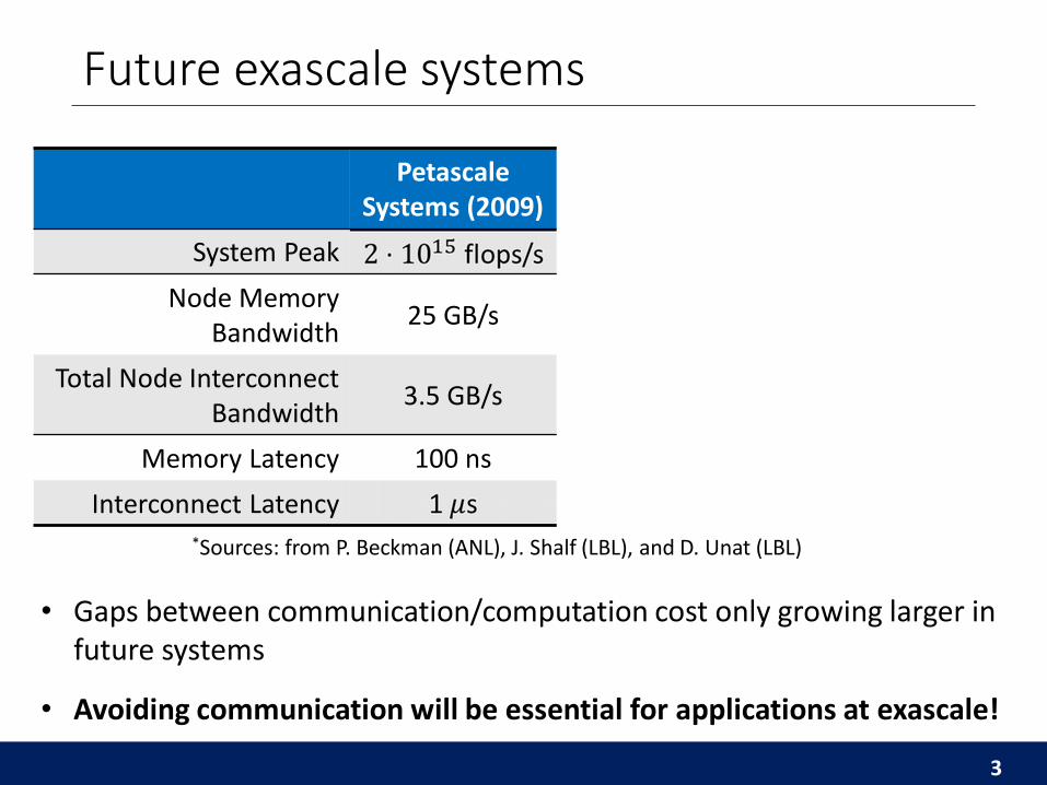
Future exascale systems
PetascaleSystems (2009)
Predicted ExascaleSystems
Factor Improvement
System Peak ~1000
Node Memory Bandwidth
25 GB/s 0.4-4 TB/s ~10-100
Total Node Interconnect Bandwidth
3.5 GB/s 100-400 GB/s ~100
Memory Latency 100 ns 50 ns ~1
Interconnect Latency ~1
3
• Gaps between communication/computation cost only growing larger in future systems
*Sources: from P. Beckman (ANL), J. Shalf (LBL), and D. Unat (LBL)
• Avoiding communication will be essential for applications at exascale!
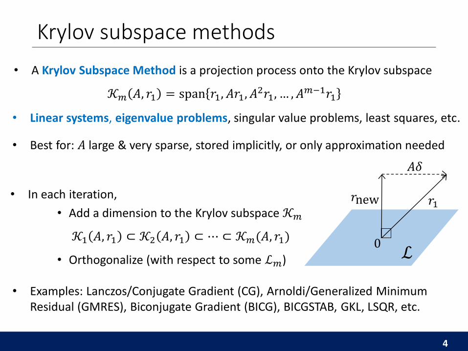
Krylov subspace methods
4
• In each iteration,
• Add a dimension to the Krylov subspace 𝒦𝑚
𝒦1 𝐴, 𝑟1 ⊂ 𝒦2 𝐴, 𝑟1 ⊂ ⋯ ⊂ 𝒦𝑚(𝐴, 𝑟1)
• Orthogonalize (with respect to some ℒ𝑚)
• Examples: Lanczos/Conjugate Gradient (CG), Arnoldi/Generalized Minimum Residual (GMRES), Biconjugate Gradient (BICG), BICGSTAB, GKL, LSQR, etc.
• A Krylov Subspace Method is a projection process onto the Krylov subspace
𝒦𝑚 𝐴, 𝑟1 = span 𝑟1, 𝐴𝑟1, 𝐴2𝑟1, … , 𝐴𝑚−1𝑟1
• Linear systems, eigenvalue problems, singular value problems, least squares, etc.
• Best for: 𝐴 large & very sparse, stored implicitly, or only approximation needed
ℒ
𝑟new
𝐴𝛿
𝑟1
0

Communication bottleneck
“Orthogonalize (with respect to some ℒ𝑚)”
Inner products
• Parallel: global reduction (MPI All-Reduce)• Sequential: multiple reads/writes to slow memory
Projection process in terms of communication:
“Add a dimension to 𝒦𝑚” Sparse matrix-vector multiplication (SpMV)• Parallel: comm. vector entries w/ neighbors• Sequential: read 𝐴/vectors from slow memory
Dependencies between communication-bound kernels in each iteration limit performance!
SpMV
orthogonalize
5
×
×
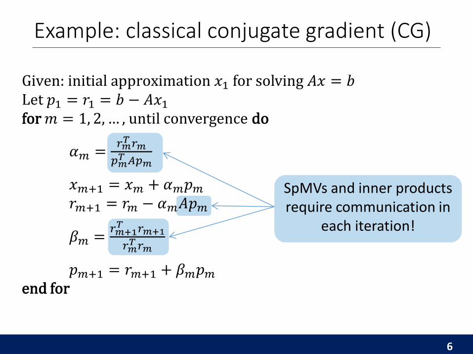
Example: classical conjugate gradient (CG)
SpMVs and inner products require communication in
each iteration!
6
Given: initial approximation 𝑥1 for solving 𝐴𝑥 = 𝑏Let 𝑝1 = 𝑟1 = 𝑏 − 𝐴𝑥1
for 𝑚 = 1, 2, … , until convergence do
𝛼𝑚 =𝑟𝑚
𝑇 𝑟𝑚
𝑝𝑚𝑇 𝐴𝑝𝑚
𝑥𝑚+1 = 𝑥𝑚 + 𝛼𝑚𝑝𝑚
𝑟𝑚+1 = 𝑟𝑚 − 𝛼𝑚𝐴𝑝𝑚
𝛽𝑚 =𝑟𝑚+1
𝑇 𝑟𝑚+1
𝑟𝑚𝑇 𝑟𝑚
𝑝𝑚+1 = 𝑟𝑚+1 + 𝛽𝑚𝑝𝑚
end for
7
0.00
0.25
0.50
0.75
1.00
1.25
1.50
1.75
0 512 1024 1536 2048 2560 3072 3584 4096
Tim
e (
seco
nd
s)
Processes (6 threads each)
Bottom Solver Time (total)
MPI_AllReduce Time (total)
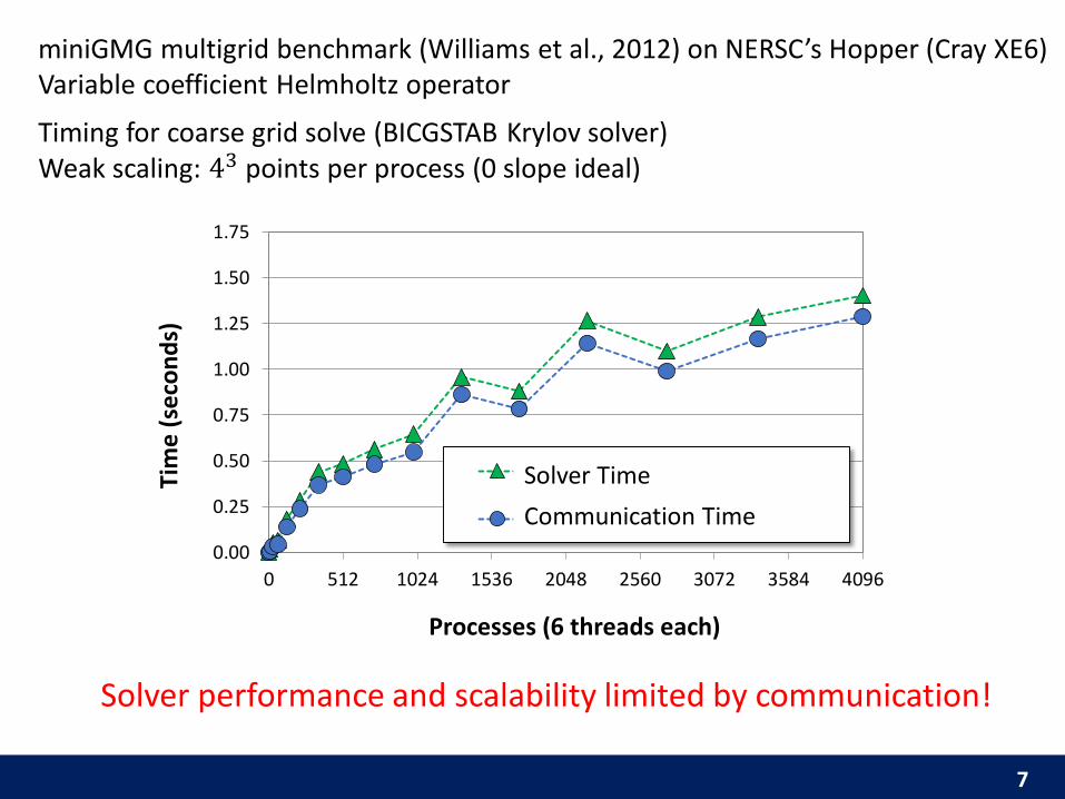
Solver Time
Communication Time
Solver performance and scalability limited by communication!
miniGMG multigrid benchmark (Williams et al., 2012) on NERSC’s Hopper (Cray XE6)Variable coefficient Helmholtz operator
Timing for coarse grid solve (BICGSTAB Krylov solver)Weak scaling: 43 points per process (0 slope ideal)

• Krylov subspace methods can be reorganized to reduce communication cost by 𝑶(𝒔)
• “Communication cost”: latency in parallel, latency and bandwidth in sequential
• Compute iteration updates in blocks of size 𝑠
• Communicate once every 𝑠 iterations instead of every iteration
• Called “s-step” or “communication-avoiding” Krylov subspace methods
• Lots of related work…
s-step Krylov subspace methods
8
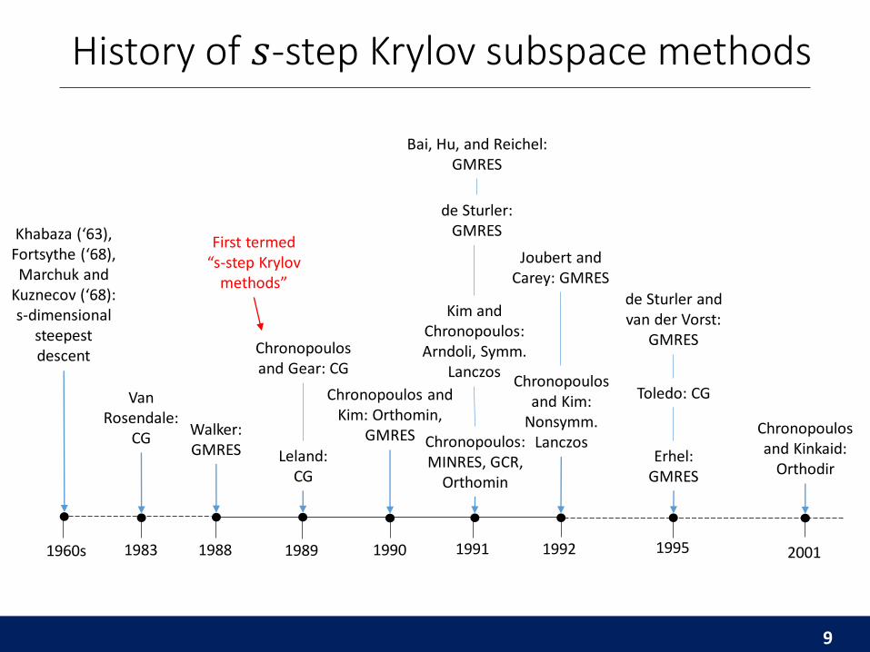
History of 𝑠-step Krylov subspace methods
9
1983
Van Rosendale:
CG
1988
Walker: GMRES
Chronopoulosand Gear: CG
1990 1991 1992
First termed “s-step Krylov
methods”
de Sturler: GMRES
1989
Bai, Hu, and Reichel:GMRES
Chronopoulosand Kim:
Nonsymm. Lanczos
Joubert and Carey: GMRES
Erhel:GMRES
Toledo: CG
de Sturler and van der Vorst:
GMRES
1995 2001
Chronopoulosand Kinkaid:
Orthodir
Chronopoulos and Kim: Orthomin,
GMRES Chronopoulos: MINRES, GCR,
Orthomin
Kim and Chronopoulos: Arndoli, Symm.
Lanczos
Leland: CG
1960s
Khabaza (‘63), Fortsythe (‘68), Marchuk and
Kuznecov (‘68): s-dimensional
steepest descent

Main idea: Unroll iteration loop by a factor of 𝑠; split iteration loop into outer 𝑘 and inner loop 𝑗 . By induction, for 𝑗 ∈ 1, … , 𝑠 + 1
𝑥𝑠𝑘+𝑗 − 𝑥𝑠𝑘+1, 𝑟𝑠𝑘+𝑗 , 𝑝𝑠𝑘+𝑗 ∈ 𝒦𝑠+1 𝐴, 𝑝𝑠𝑘+1 + 𝒦𝑠 𝐴, 𝑟𝑠𝑘+1
Brief derivation of s-step CG
11
Outer loop: Communication step
Expand solution space 𝒔 dimensions at once• Compute “basis” matrix 𝒴𝑘 whose cols. span 𝒦𝑠+1 𝐴, 𝑝𝑠𝑘+1 + 𝒦𝑠 𝐴, 𝑟𝑠𝑘+1
• If 𝐴𝑠 is well partitioned, requires reading 𝑨/communicating vectors only onceusing matrix powers kernel (Demmel et al.,‘07)
Orthogonalize all at once:
• Encode inner products between basis vectors with Gram matrix 𝒢𝑘 = 𝒴𝑘𝑇𝒴𝑘
(or compute Tall-Skinny QR) • Communication cost of one global reduction
13
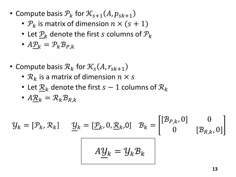
• Compute basis 𝒫𝑘 for 𝒦𝑠+1 𝐴, 𝑝𝑠𝑘+1
• 𝒫𝑘 is matrix of dimension 𝑛 × (𝑠 + 1)
• Let 𝒫𝑘 denote the first 𝑠 columns of 𝒫𝑘
• 𝐴𝒫𝑘 = 𝒫𝑘ℬ𝑃,𝑘
• Compute basis ℛ𝑘 for 𝒦𝑠 𝐴, 𝑟𝑠𝑘+1
• ℛ𝑘 is a matrix of dimension 𝑛 × 𝑠
• Let ℛ𝑘 denote the first 𝑠 − 1 columns of ℛ𝑘
• 𝐴ℛ𝑘 = ℛ𝑘ℬ𝑅,𝑘
𝒴𝑘 = [𝒫𝑘, ℛ𝑘] 𝒴𝑘 = [𝒫𝑘 , 0, ℛ𝑘,0] ℬ𝑘 =[ℬ𝑃,𝑘, 0] 0
0 [ℬ𝑅,𝑘, 0]
𝐴𝒴𝑘 = 𝒴𝑘ℬ𝑘
9
→
→
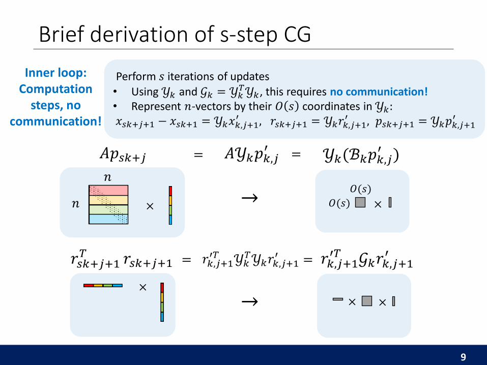
Perform 𝑠 iterations of updates
• Using 𝒴𝑘 and 𝒢𝑘 = 𝒴𝑘𝑇𝒴𝑘 , this requires no communication!
• Represent 𝑛-vectors by their 𝑂 𝑠 coordinates in 𝒴𝑘:𝑥𝑠𝑘+𝑗+1 − 𝑥𝑠𝑘+1 = 𝒴𝑘𝑥𝑘,𝑗+1
′ , 𝑟𝑠𝑘+𝑗+1 = 𝒴𝑘𝑟𝑘,𝑗+1′ , 𝑝𝑠𝑘+𝑗+1 = 𝒴𝑘𝑝𝑘,𝑗+1
′
𝒴𝑘(ℬ𝑘𝑝𝑘,𝑗′ )
𝑂(𝑠)
𝑂(𝑠)
×
𝑟𝑘,𝑗+1′𝑇 𝒢𝑘𝑟𝑘,𝑗+1
′
× ×
Inner loop:Computation
steps, no communication!
𝑟𝑠𝑘+𝑗+1𝑇 𝑟𝑠𝑘+𝑗+1
𝐴𝑝𝑠𝑘+𝑗
×
×𝑛
𝑛
𝐴𝒴𝑘𝑝𝑘,𝑗′
= =
= 𝑟𝑘,𝑗+1′𝑇 𝒴𝑘
𝑇𝒴𝑘𝑟𝑘,𝑗+1′ =
Brief derivation of s-step CG

via Matrix Powers Kernel
Global reduction
to compute 𝒢𝑘
15
s-step CG
Local computations within inner loop require
no communication!
Given: initial approximation 𝑥1 for solving 𝐴𝑥 = 𝑏Let 𝑝1 = 𝑟1 = 𝑏 − 𝐴𝑥1
for k = 0, 1, … , until convergence doCompute 𝒴𝑘 such that 𝐴𝒴𝑘 = 𝒴𝑘ℬ𝑘 , compute 𝒢𝑘 = 𝒴𝑘
𝑇𝒴𝑘
Let 𝑥𝑘,1′ = 02𝑠+1, 𝑟𝑘,1
′ = 𝑒𝑠+2, 𝑝𝑘,1′ = 𝑒1
for 𝑗 = 1, … , 𝑠 do
𝛼𝑠𝑘+𝑗 =𝑟𝑘,𝑗
′𝑇𝒢𝑘𝑟𝑘,𝑗′
𝑝𝑘,𝑗′𝑇 𝒢𝑘ℬ𝑘𝑝𝑘,𝑗
′
𝑥𝑘,𝑗+1′ = 𝑥𝑘,𝑗
′ + 𝛼𝑠𝑘+𝑗𝑝𝑘,𝑗′
𝑟𝑘,𝑗+1′ = 𝑟𝑘,𝑗
′ − 𝛼𝑠𝑘+𝑗ℬ𝑘𝑝𝑘,𝑗′
𝛽𝑠𝑘+𝑗 =𝑟𝑘,𝑗+1
′𝑇 𝒢𝑘𝑟𝑘,𝑗+1′
𝑟𝑘,𝑗′𝑇𝒢𝑘𝑟𝑘,𝑗
′
𝑝𝑘,𝑗+1′ = 𝑟𝑘,𝑗+1
′ + 𝛽𝑠𝑘+𝑗𝑝𝑘,𝑗′
end for𝑥𝑠𝑘+𝑠+1 = 𝒴𝑘𝑥𝑘,𝑠+1
′ + 𝑥𝑠𝑘+1, 𝑟𝑠𝑘+𝑠+1 = 𝒴𝑘𝑟𝑘,𝑠+1′ , 𝑝𝑠𝑘+𝑠+1 = 𝒴𝑘𝑝𝑘,𝑠+1
′
end for

Complexity comparison
16
Example of parallel (per processor) complexity for 𝑠 iterations of CG vs. s-step CG for a 2D 9-point stencil:
(Assuming each of 𝑝 processors owns 𝑛/𝑝 rows of the matrix and 𝑠 ≤ 𝑛/𝑝)
All values in the table meant in the Big-O sense (i.e., lower order terms and constants not included)
Flops Words Moved Messages
SpMV Orth. SpMV Orth. SpMV Orth.
Classical CG
𝑠𝑛
𝑝
𝑠𝑛
𝑝 𝑠 𝑛 𝑝 𝑠 log2 𝑝 𝑠 𝑠 log2 𝑝
s-step CG𝑠𝑛
𝑝𝑠2𝑛
𝑝𝑠 𝑛 𝑝 𝑠2 log2 𝑝 1 log2 𝑝
Tradeoffs
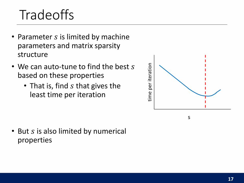
• Parameter 𝑠 is limited by machine parameters and matrix sparsitystructure
• We can auto-tune to find the best 𝑠based on these properties
• That is, find 𝑠 that gives the least time per iteration
• But 𝑠 is also limited by numerical properties
17
tim
e p
er it
erat
ion
s
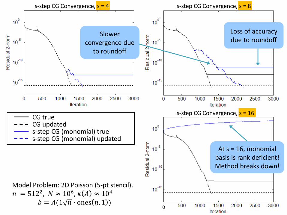
s-step CG Convergence, s = 4 s-step CG Convergence, s = 8
0
s-step CG Convergence, s = 16
Slower convergence due
to roundoff
Loss of accuracy due to roundoff
At s = 16, monomial basis is rank deficient! Method breaks down!
CG trueCG updateds-step CG (monomial) trues-step CG (monomial) updated
Model Problem: 2D Poisson (5-pt stencil), 𝑛 = 5122, 𝑁 ≈ 106, 𝜅 𝐴 ≈ 104
𝑏 = 𝐴(1 𝑛 ⋅ ones 𝑛, 1 )
Behavior in finite precision
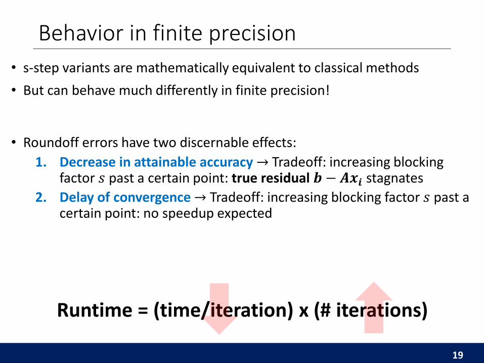
• s-step variants are mathematically equivalent to classical methods
• But can behave much differently in finite precision!
• Roundoff errors have two discernable effects:
1. Decrease in attainable accuracy → Tradeoff: increasing blocking factor 𝑠 past a certain point: true residual 𝒃 − 𝑨𝒙𝒊 stagnates
2. Delay of convergence → Tradeoff: increasing blocking factor 𝑠 past a certain point: no speedup expected
19
Runtime = (time/iteration) x (# iterations)

• Selecting the best 𝑠 to use (minimize runtime subject to accuracy constraint) is a hard problem
• Can tune to minimize time per iteration (based on hardware, matrix structure)
• But numerical properties (stability, convergence rate) are important too!
• The “best” 𝑠 for minimizing time per iteration might not be the best 𝑠 for minimizing overall runtime, and might give an inaccurate solution
• Goal: Based on finite precision analysis, develop ways to automate parameter choice to improve reliability and usability of s-step Krylovsubspace methods
• Improving s-step basis conditioning
• Residual replacement
• Variable s-step methods
20
Optimizing for speed and accuracy
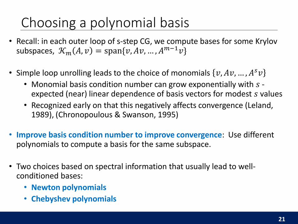
Choosing a polynomial basis• Recall: in each outer loop of s-step CG, we compute bases for some Krylov
subspaces, 𝒦𝑚 𝐴, 𝑣 = span{𝑣, 𝐴𝑣, … , 𝐴𝑚−1𝑣}
• Simple loop unrolling leads to the choice of monomials 𝑣, 𝐴𝑣, … , 𝐴𝑠𝑣
• Monomial basis condition number can grow exponentially with 𝑠 -expected (near) linear dependence of basis vectors for modest 𝑠 values
• Recognized early on that this negatively affects convergence (Leland, 1989), (Chronopoulous & Swanson, 1995)
• Improve basis condition number to improve convergence: Use different polynomials to compute a basis for the same subspace.
• Two choices based on spectral information that usually lead to well-conditioned bases:
• Newton polynomials
• Chebyshev polynomials
21
Better conditioned bases
22
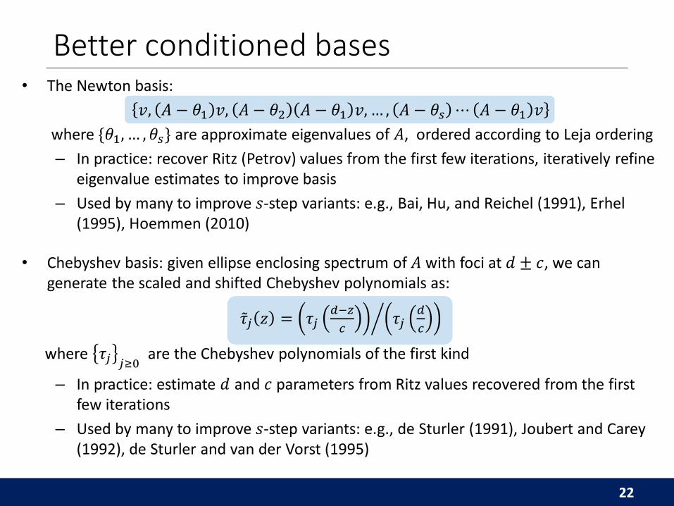
• The Newton basis:
𝑣, 𝐴 − 𝜃1 𝑣, 𝐴 − 𝜃2 𝐴 − 𝜃1 𝑣, … , 𝐴 − 𝜃𝑠 ⋯ 𝐴 − 𝜃1 𝑣
where {𝜃1, … , 𝜃𝑠} are approximate eigenvalues of 𝐴, ordered according to Leja ordering
– In practice: recover Ritz (Petrov) values from the first few iterations, iteratively refine eigenvalue estimates to improve basis
– Used by many to improve 𝑠-step variants: e.g., Bai, Hu, and Reichel (1991), Erhel (1995), Hoemmen (2010)
• Chebyshev basis: given ellipse enclosing spectrum of 𝐴 with foci at 𝑑 ± 𝑐, we can generate the scaled and shifted Chebyshev polynomials as:
𝜏𝑗 𝑧 = 𝜏𝑗𝑑−𝑧
𝑐𝜏𝑗
𝑑
𝑐
where 𝜏𝑗 𝑗≥0are the Chebyshev polynomials of the first kind
– In practice: estimate 𝑑 and 𝑐 parameters from Ritz values recovered from the first few iterations
– Used by many to improve 𝑠-step variants: e.g., de Sturler (1991), Joubert and Carey (1992), de Sturler and van der Vorst (1995)
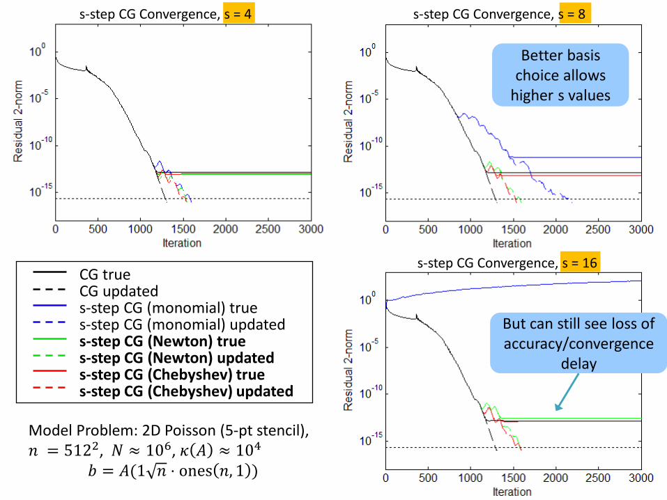
Better basis choice allows
higher s values
s-step CG Convergence, s = 4 s-step CG Convergence, s = 8
s-step CG Convergence, s = 16
But can still see loss of accuracy/convergence
delay
CG trueCG updateds-step CG (monomial) trues-step CG (monomial) updateds-step CG (Newton) trues-step CG (Newton) updateds-step CG (Chebyshev) trues-step CG (Chebyshev) updated
Model Problem: 2D Poisson (5-pt stencil), 𝑛 = 5122, 𝑁 ≈ 106, 𝜅 𝐴 ≈ 104
𝑏 = 𝐴(1 𝑛 ⋅ ones 𝑛, 1 )

Maximum attainable accuracy of CG
24
• In classical CG, iterates are updated by
𝑥𝑚+1 = 𝑥𝑚 + 𝛼𝑚 𝑝𝑚 + 𝜉𝑚+1 and 𝑟𝑚+1 = 𝑟𝑚 − 𝛼𝑚𝐴 𝑝𝑚 + 𝜂𝑚+1
• Accumulation of rounding errors cause the true residual, 𝒃 − 𝑨 𝒙𝒎+𝟏, and the updated residual, 𝒓𝒎+𝟏, to deviate
• The size of the true residual:
𝑏 − 𝐴 𝑥𝑚+1 ≤ 𝑟𝑚+1 + 𝑏 − 𝐴 𝑥𝑚+1 − 𝑟𝑚+1
• As 𝑟𝑚+1 → 0, 𝑏 − 𝐴 𝑥𝑚+1 depends on 𝑏 − 𝐴 𝑥𝑚+1 − 𝑟𝑚+1
• Many results on attainable accuracy, e.g.: Greenbaum (1989, 1994, 1997), Sleijpen, van der Vorst and Fokkema (1994), Sleijpen, van der Vorst and Modersitzki (2001), Björck, Elfving and Strakoš (1998) and Gutknecht and Strakoš (2000).
• Can perform a similar analysis to upper bound the maximum attainable accuracy in finite precision s-step CG

Error in basis change
Sources of roundoff error in s-step CG
Error in computing 𝑠-step basis
Error in updating coefficient vectors
25
Computing the 𝑠-step Krylov basis:
𝐴 𝒴𝑘 = 𝒴𝑘ℬ𝑘 + ∆𝑘
Updating coordinate vectors in the inner loop:
𝑥𝑘,𝑗+1′ = 𝑥𝑘,𝑗
′ + 𝑞𝑘,𝑗′ + 𝜉𝑘,𝑗+1
𝑟𝑘,𝑗+1′ = 𝑟𝑘,𝑗
′ − ℬ𝑘 𝑞𝑘,𝑗′ + 𝜂𝑘,𝑗+1
with 𝑞𝑘,𝑗′ = fl( 𝛼𝑠𝑘+𝑗 𝑝𝑘,𝑗
′ )
Recovering CG vectors for use in next outer loop:
𝑥𝑠𝑘+𝑗+1 = 𝒴𝑘 𝑥𝑘,𝑗+1′ + 𝑥𝑠𝑘+1 + 𝜙𝑠𝑘+𝑗+1
𝑟𝑠𝑘+𝑗+1 = 𝒴𝑘 𝑟𝑘,𝑗+1′ + 𝜓𝑠𝑘+𝑗+1
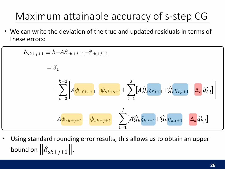
𝛿𝑠𝑘+𝑗+1 ≡ 𝑏−𝐴 𝑥𝑠𝑘+𝑗+1− 𝑟𝑠𝑘+𝑗+1
= 𝛿1
−
ℓ=0
𝑘−1
𝐴𝜙𝑠ℓ+𝑠+1+𝜓𝑠ℓ+𝑠+1+
𝑖=1
𝑠
𝐴 𝒴ℓ𝜉ℓ,𝑖+1+ 𝒴ℓ𝜂ℓ,𝑖+1 −Δℓ 𝑞ℓ,𝑖′
−𝐴𝜙𝑠𝑘+𝑗+1 − 𝜓𝑠𝑘+𝑗+1 −
𝑖=1
𝑗
𝐴 𝒴𝑘𝜉𝑘,𝑖+1+ 𝒴𝑘𝜂𝑘,𝑖+1 − Δ𝑘 𝑞𝑘,𝑖′
• We can write the deviation of the true and updated residuals in terms of these errors:
Maximum attainable accuracy of s-step CG
• Using standard rounding error results, this allows us to obtain an upper
bound on 𝛿𝑠𝑘+𝑗+1 .
26

For CG:
Attainable accuracy of CG versus s-step CG
27
𝛿𝑠𝑘+𝑗+1 ≤ 𝛿1 + 휀𝒄 𝚪𝒌
𝑖=1
𝑠𝑘+𝑗
1 + 𝑁 𝐴 𝑥𝑖+1 + 𝑟𝑖+1
𝛿𝑚+1 ≤ 𝛿1 + 휀
𝑖=1
𝑚
1 + 𝑁 𝐴 𝑥𝑖+1 + 𝑟𝑖+1
For s-step CG:
where 𝑐 is a low-degree polynomial in 𝑠, and
Γ𝑘 = maxℓ≤𝑘
Γℓ , where Γℓ = 𝒴ℓ+ ⋅ 𝒴ℓ
Residual replacement strategy
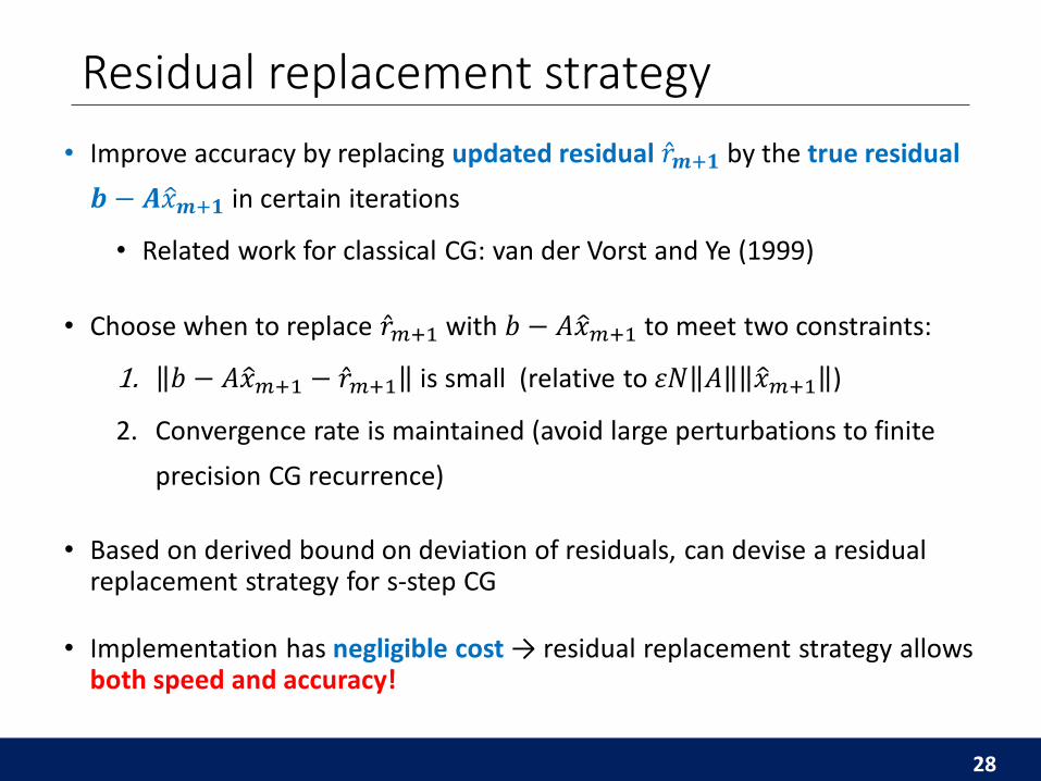
• Improve accuracy by replacing updated residual 𝑟𝒎+𝟏 by the true residual
𝒃 − 𝑨 𝑥𝒎+𝟏 in certain iterations
• Related work for classical CG: van der Vorst and Ye (1999)
28
• Based on derived bound on deviation of residuals, can devise a residual replacement strategy for s-step CG
• Choose when to replace 𝑟𝑚+1 with 𝑏 − 𝐴 𝑥𝑚+1 to meet two constraints:
1. 𝑏 − 𝐴 𝑥𝑚+1 − 𝑟𝑚+1 is small (relative to 휀𝑁 𝐴 𝑥𝑚+1 )
2. Convergence rate is maintained (avoid large perturbations to finite
precision CG recurrence)
• Implementation has negligible cost → residual replacement strategy allows both speed and accuracy!

if 𝑑𝑠𝑘+𝑗 ≤ 휀 𝑟𝑠𝑘+𝑗 𝐚𝐧𝐝 𝑑𝑠𝑘+𝑗+1 > 휀 𝑟𝑠𝑘+𝑗+1 𝐚𝐧𝐝 𝑑𝑠𝑘+𝑗+1 > 1.1𝑑𝑖𝑛𝑖𝑡
𝑧 = 𝑧 + 𝒴𝑘 𝑥𝑘,𝑗+1′ + 𝑥𝑠𝑘+1
𝑥𝑠𝑘+𝑗+1 = 0
𝑟𝑠𝑘+𝑗+1 = 𝑏 − 𝐴𝑧
𝑑𝑖𝑛𝑖𝑡 = 𝑑𝑠𝑘+𝑗+1= 휀 1 + 2𝑁′ 𝐴 𝑧 + 𝑟𝑠𝑘+𝑗+1
𝑝𝑠𝑘+𝑗+1 = 𝒴𝑘𝑝𝑘,𝑗+1′
break from inner loop and begin new outer loop
end
Residual replacement for s-step CG
• Use computable bound for 𝑏 − 𝐴𝑥𝑠𝑘+𝑗+1 − 𝑟𝑠𝑘+𝑗+1 to update 𝑑𝑠𝑘+𝑗+1, an estimate of error in computing 𝑟𝑠𝑘+𝑗+1, in each iteration
• Set threshold 휀 ≈ 휀, replace whenever 𝑑𝑠𝑘+𝑗+1/ 𝑟𝑠𝑘+𝑗+1 reaches threshold
29
Pseudo-code for residual replacement with group update for s-step CG:
group update of approximate solution
set residual to true residual
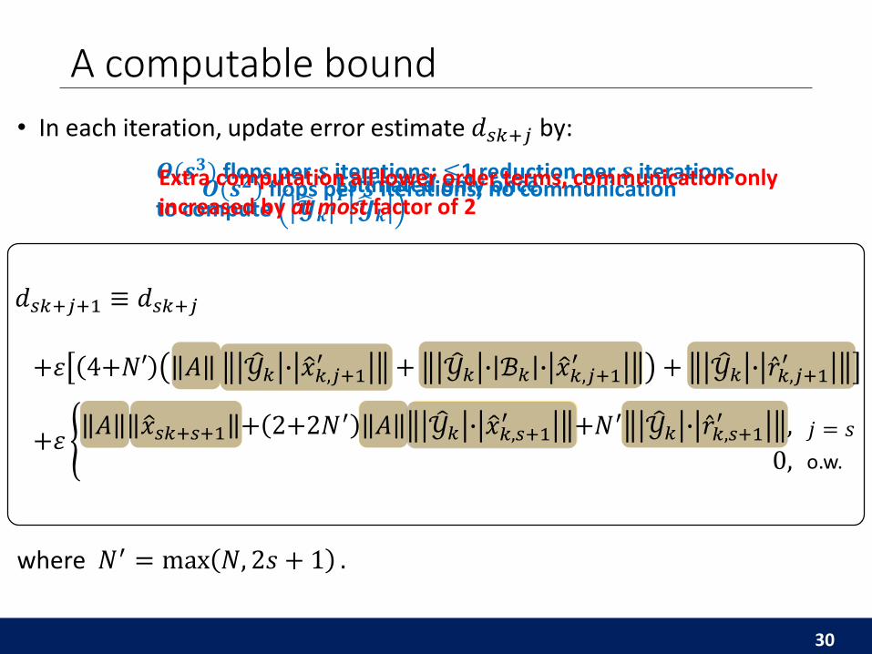
• In each iteration, update error estimate 𝑑𝑠𝑘+𝑗 by:
A computable bound
o.w.
𝑗 = 𝑠
where 𝑁′ = max 𝑁, 2𝑠 + 1 .
Estimated only once𝑶(𝒔𝟐) flops per 𝒔 iterations; no communication𝑶(𝒔𝟑) flops per 𝒔 iterations; ≤1 reduction per 𝒔 iterations
to compute 𝓨𝒌𝑻 𝓨𝒌
Extra computation all lower order terms, communication only increased by at most factor of 2
30
+휀 𝐴 𝑥𝑠𝑘+𝑠+1 + 2+2𝑁′ 𝐴 𝒴𝑘 ∙ 𝑥𝑘,𝑠+1
′ +𝑁′ 𝒴𝑘 ∙ 𝑟𝑘,𝑠+1′ ,
0,
𝑑𝑠𝑘+𝑗+1 ≡ 𝑑𝑠𝑘+𝑗
+휀 4+𝑁′ 𝐴 𝒴𝑘 ∙ 𝑥𝑘,𝑗+1′ + 𝒴𝑘 ∙ ℬ𝑘 ∙ 𝑥𝑘,𝑗+1
′ + 𝒴𝑘 ∙ 𝑟𝑘,𝑗+1′
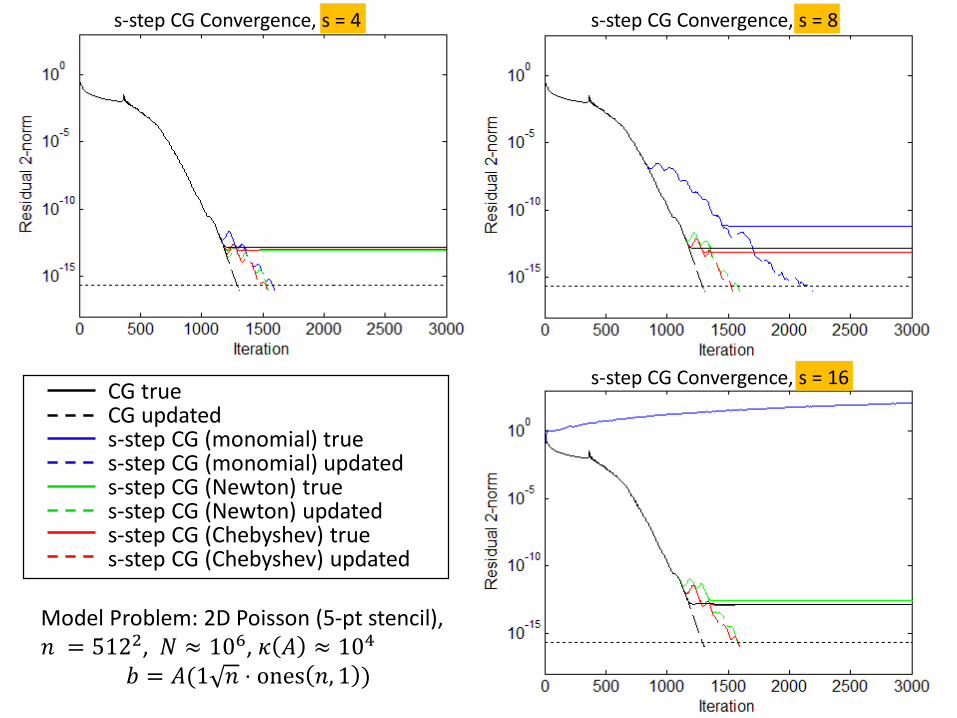
s-step CG Convergence, s = 4 s-step CG Convergence, s = 8
s-step CG Convergence, s = 16CG trueCG updateds-step CG (monomial) trues-step CG (monomial) updateds-step CG (Newton) trues-step CG (Newton) updateds-step CG (Chebyshev) trues-step CG (Chebyshev) updated
Model Problem: 2D Poisson (5-pt stencil), 𝑛 = 5122, 𝑁 ≈ 106, 𝜅 𝐴 ≈ 104
𝑏 = 𝐴(1 𝑛 ⋅ ones 𝑛, 1 )
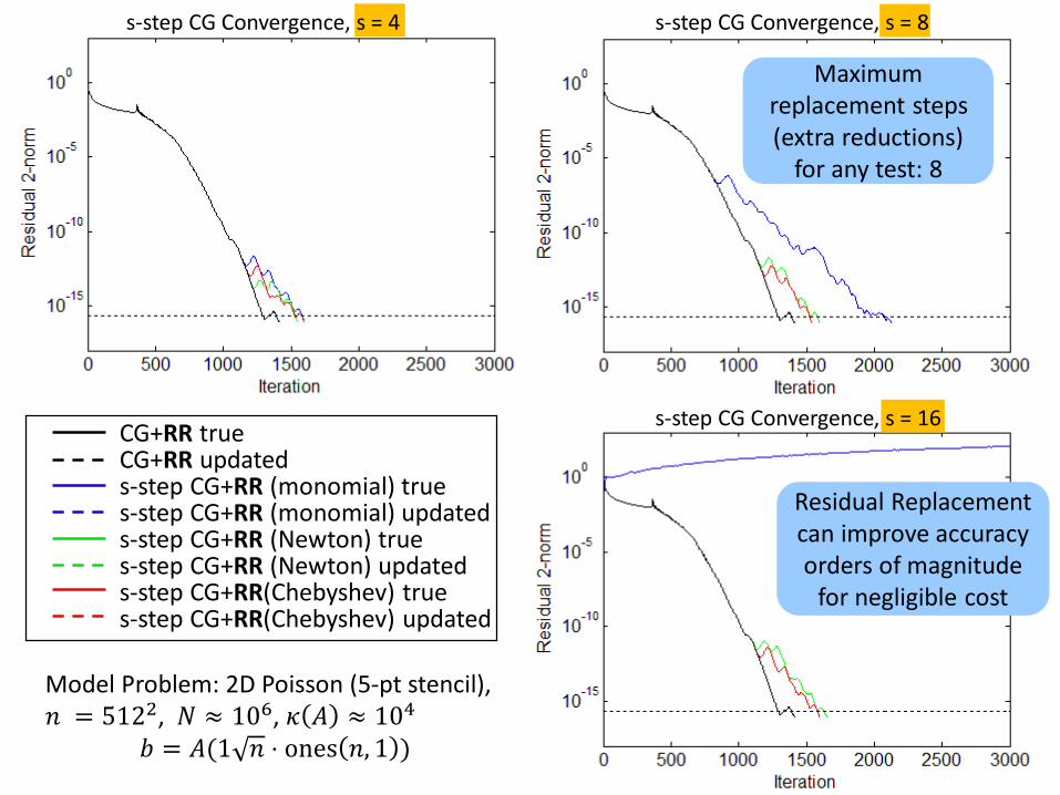
s-step CG Convergence, s = 4 s-step CG Convergence, s = 8
s-step CG Convergence, s = 16CG+RR trueCG+RR updateds-step CG+RR (monomial) trues-step CG+RR (monomial) updateds-step CG+RR (Newton) trues-step CG+RR (Newton) updateds-step CG+RR(Chebyshev) trues-step CG+RR(Chebyshev) updated
Residual Replacement can improve accuracy orders of magnitude
for negligible cost
Maximum replacement steps (extra reductions)
for any test: 8
Model Problem: 2D Poisson (5-pt stencil), 𝑛 = 5122, 𝑁 ≈ 106, 𝜅 𝐴 ≈ 104
𝑏 = 𝐴(1 𝑛 ⋅ ones 𝑛, 1 )
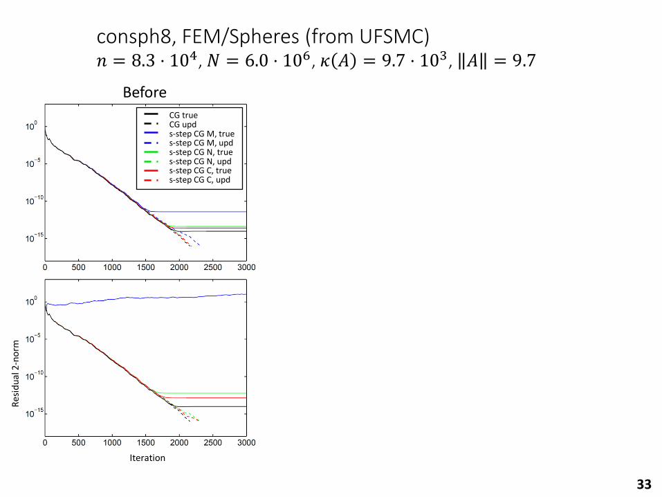
consph8, FEM/Spheres (from UFSMC)𝑛 = 8.3 ⋅ 104, 𝑁 = 6.0 ⋅ 106, 𝜅 𝐴 = 9.7 ⋅ 103, 𝐴 = 9.7
33
Before After
𝑠=
8𝑠
=1
2
Class. 2
Mono. 12
Newt. 2
Cheb. 2
# Replacements
Class. 2
Mono. 0
Newt. 4
Cheb. 3
# Replacements
CG+RR trueCG+RR upds-step CG+RR M, trues-step CG+RR M, upds-step CG+RR N, trues-step CG+RR N, upds-step CG+RR C, trues-step CG+RR C, upd
CG trueCG upds-step CG M, trues-step CG M, upds-step CG N, trues-step CG N, upds-step CG C, trues-step CG C, upd
Res
idu
al 2
-no
rm
Iteration

• Consider the growth of the relative residual gap caused by errors in outer loop 𝑘
• We can approximate an upper bound on this quantity by
𝛿𝑠𝑘+𝑠+1 − 𝛿𝑠𝑘+1
𝐴 𝑥≲ 𝑐𝜅 𝐴 Γ𝑘휀
𝑟𝑠𝑘+1
𝐴 𝑥
where 𝑐 is a low-degree polynomial in 𝑠
• If our application requires relative accuracy 휀∗, we must have
Γ𝑘 ≡ 𝒴𝑘+ 𝒴𝑘 ≲
휀∗ 𝑏
𝑐휀 𝑟𝑠𝑘+1
• In other words, as the method converges (i.e., as 𝑟𝑠𝑘+1 decreases), we can tolerate more ill-conditioned s-step bases without affecting attainable accuracy
• This naturally leads to a variable s-step approach, where 𝑠 starts off small and increases as the method converges
• Analogy to relaxation strategy in “inexact Krylov subspace methods”
Variable s-step CG derivation
34
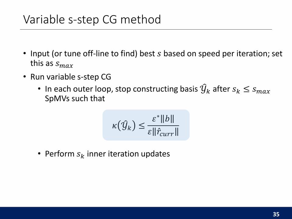
• Input (or tune off-line to find) best 𝑠 based on speed per iteration; set this as 𝑠𝑚𝑎𝑥
• Run variable s-step CG
• In each outer loop, stop constructing basis 𝒴𝑘 after 𝑠𝑘 ≤ 𝑠𝑚𝑎𝑥SpMVs such that
𝜅 𝒴𝑘 ≤휀∗ 𝑏
휀 𝑟𝑐𝑢𝑟𝑟
• Perform 𝑠𝑘 inner iteration updates
Variable s-step CG method
35
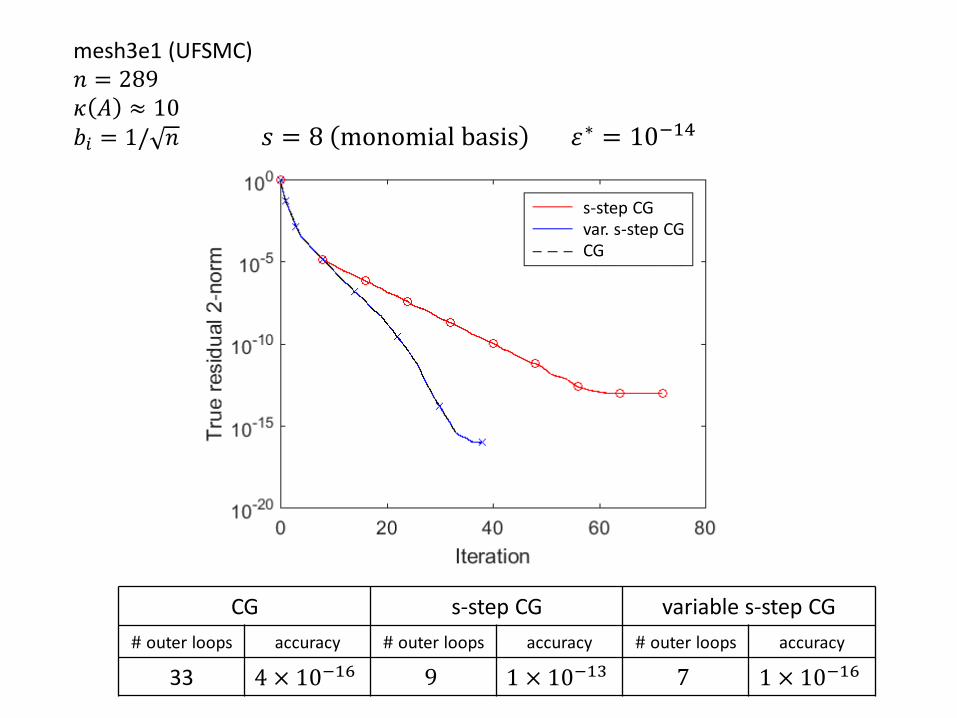
𝑠 = 8 monomial basis 휀∗ = 10−14
CG s-step CG variable s-step CG
# outer loops accuracy # outer loops accuracy # outer loops accuracy
33 4 × 10⁻¹⁶ 9 1 × 10⁻¹³ 7 1 × 10⁻¹⁶
mesh3e1 (UFSMC)𝑛 = 289𝜅 𝐴 ≈ 10𝑏𝑖 = 1/ 𝑛
s-step CGvar. s-step CGCG
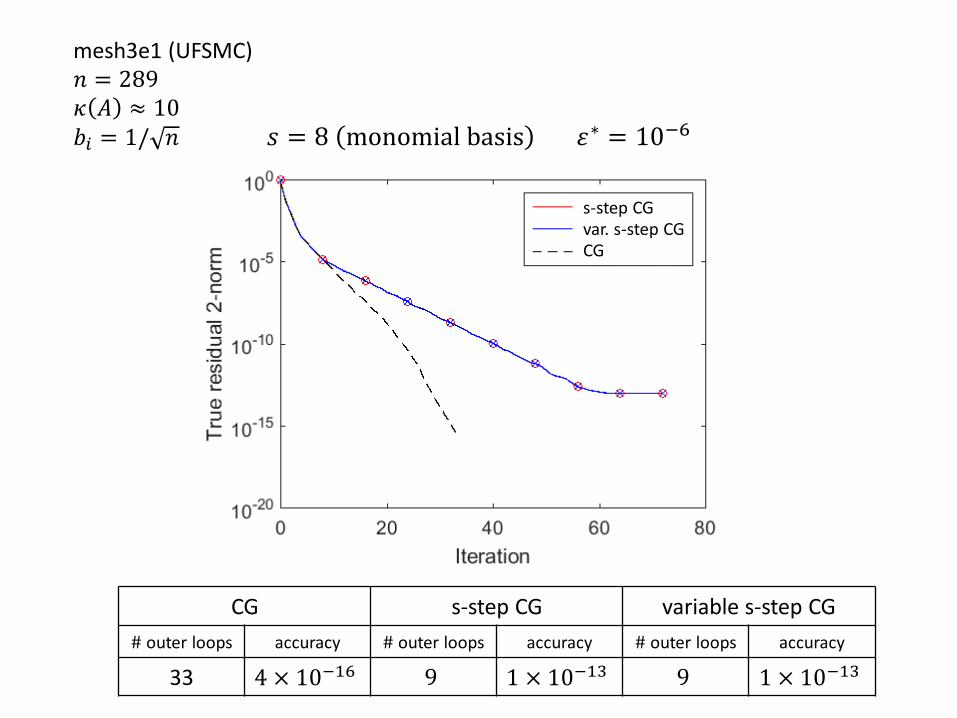
CG s-step CG variable s-step CG
# outer loops accuracy # outer loops accuracy # outer loops accuracy
33 4 × 10⁻¹⁶ 9 1 × 10⁻¹³ 9 1 × 10⁻¹³
𝑠 = 8 monomial basis 휀∗ = 10−6
s-step CGvar. s-step CGCG
mesh3e1 (UFSMC)𝑛 = 289𝜅 𝐴 ≈ 10𝑏𝑖 = 1/ 𝑛
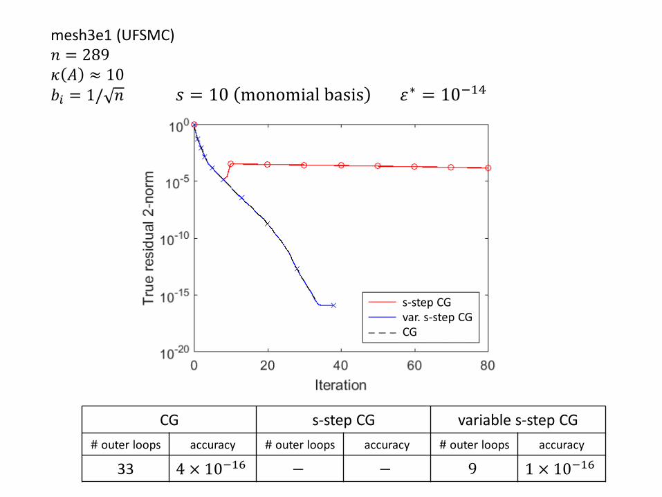
𝑠 = 10 monomial basis 휀∗ = 10−14
CG s-step CG variable s-step CG
# outer loops accuracy # outer loops accuracy # outer loops accuracy
33 4 × 10⁻¹⁶ − − 9 1 × 10⁻¹⁶
s-step CGvar. s-step CGCG
mesh3e1 (UFSMC)𝑛 = 289𝜅 𝐴 ≈ 10𝑏𝑖 = 1/ 𝑛
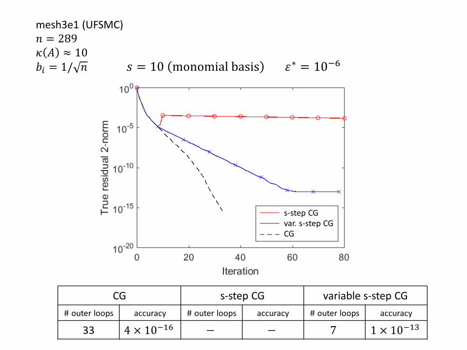
𝑠 = 10 monomial basis 휀∗ = 10−6
CG s-step CG variable s-step CG
# outer loops accuracy # outer loops accuracy # outer loops accuracy
33 4 × 10⁻¹⁶ − − 7 1 × 10⁻¹³
s-step CGvar. s-step CGCG
mesh3e1 (UFSMC)𝑛 = 289𝜅 𝐴 ≈ 10𝑏𝑖 = 1/ 𝑛

ex5 (UFSMC)𝑛 = 27𝜅 𝐴 ≈ 7 × 10⁷
𝑏𝑖 = 1/ 𝑛 𝑠 = 10 monomial basis 휀∗ = 10−14
CG s-step CG variable s-step CG
# outer loops accuracy # outer loops accuracy # outer loops accuracy
157 9 × 10⁻⁹ − − 60 5 × 10⁻⁹
s-step CGvar. s-step CGCG

Paige’s results for classical Lanczos
• Using bounds on local rounding errors in Lanczos, Paige showed that
1. The computed Ritz values always lie between the extreme eigenvalues of 𝐴 to within a small multiple of machine precision.
2. At least one small interval containing an eigenvalue of 𝐴 is found by the 𝑛th iteration.
3. The algorithm behaves numerically like Lanczos with full reorthogonalization until a very close eigenvalue approximation is found.
4. The loss of orthogonality among basis vectors follows a rigorous pattern and implies that some Ritz values have converged.
Do the same statements hold for s-step Lanczos?
41
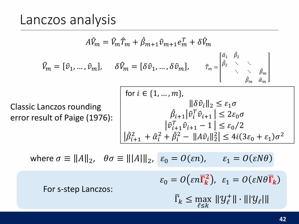
𝐴 𝑉𝑚 = 𝑉𝑚 𝑇𝑚 + 𝛽𝑚+1 𝑣𝑚+1𝑒𝑚
𝑇 + 𝛿 𝑉𝑚
𝑉𝑚 = 𝑣1, … , 𝑣𝑚 , 𝛿 𝑉𝑚 = 𝛿 𝑣1, … , 𝛿 𝑣𝑚 , 𝑇𝑚 =
𝛼1 𝛽2
𝛽2 ⋱ ⋱
⋱ ⋱ 𝛽𝑚
𝛽𝑚 𝛼𝑚
Lanczos analysis
Classic Lanczos rounding error result of Paige (1976):
for 𝑖 ∈ {1, … , 𝑚},𝛿 𝑣𝑖 2 ≤ 휀1𝜎
𝛽𝑖+1 𝑣𝑖𝑇 𝑣𝑖+1 ≤ 2휀0𝜎
𝑣𝑖+1𝑇 𝑣𝑖+1 − 1 ≤ 휀0 2
𝛽𝑖+12 + 𝛼𝑖
2 + 𝛽𝑖2 − 𝐴 𝑣𝑖 2
2 ≤ 4𝑖 3휀0 + 휀1 𝜎2
42
where 𝜎 ≡ 𝐴 2, 𝜃𝜎 ≡ 𝐴 2, 휀0 = 𝑂(휀𝑛), 휀1 = 𝑂 휀𝑁𝜃
For s-step Lanczos:휀0 = 𝑂 휀𝑛 𝚪𝒌
𝟐 , 휀1 = 𝑂 휀𝑁𝜃 𝚪𝒌
Γ𝑘 ≤ maxℓ≤𝑘
𝒴ℓ+ ∙ 𝒴ℓ
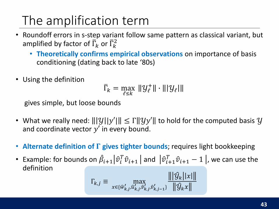
• Roundoff errors in s-step variant follow same pattern as classical variant, but amplified by factor of Γ𝑘 or Γ𝑘
2
• Theoretically confirms empirical observations on importance of basis conditioning (dating back to late ‘80s)
• Using the definition Γ𝑘 = max
ℓ≤𝑘𝒴ℓ
+ ∙ 𝒴ℓ
gives simple, but loose bounds
• What we really need: 𝒴 |𝑦′| ≤ Γ 𝒴𝑦′ to hold for the computed basis 𝒴and coordinate vector 𝑦′ in every bound.
• Alternate definition of 𝚪 gives tighter bounds; requires light bookkeeping
• Example: for bounds on 𝛽𝑖+1 𝑣𝑖𝑇 𝑣𝑖+1 and 𝑣𝑖+1
𝑇 𝑣𝑖+1 − 1 , we can use the definition
Γ𝑘,𝑗 ≡ max𝑥∈{ 𝑤𝑘,𝑗
′ , 𝑢𝑘,𝑗′ , 𝑣𝑘,𝑗
′ , 𝑣𝑘,𝑗−1′ }
𝒴𝑘 𝑥
𝒴𝑘𝑥
The amplification term
43

• The answer is YES
• 𝒴ℓ is numerically full rank for 0 ≤ ℓ ≤ 𝑘 and
• 휀0 ≡ 2휀 𝑛+11𝑠+15 Γ𝑘2 ≤
1
12
• i.e., Γ𝑘2 ≤ 24휀 𝑛 + 11𝑠 + 15
−1
• Otherwise, e.g., can lose orthogonality due to computation with rank-deficient basis
Results for s-step Lanczos
44
…if
• Back to our question: Do Paige’s results, e.g.,loss of orthogonality eigenvalue convergence
hold for s-step Lanczos?
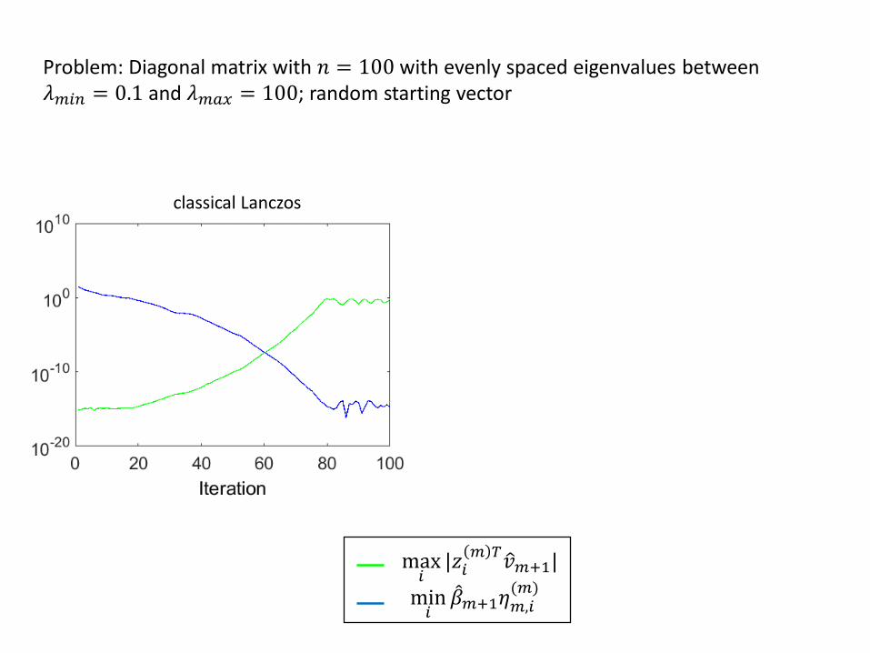
Problem: Diagonal matrix with 𝑛 = 100 with evenly spaced eigenvalues between 𝜆𝑚𝑖𝑛 = 0.1 and 𝜆𝑚𝑎𝑥 = 100; random starting vector
max𝑖
|𝑧𝑖𝑚 𝑇
𝑣𝑚+1|
min𝑖
𝛽𝑚+1𝜂𝑚,𝑖(𝑚)
classical Lanczos

Problem: Diagonal matrix with 𝑛 = 100 with evenly spaced eigenvalues between 𝜆𝑚𝑖𝑛 = 0.1 and 𝜆𝑚𝑎𝑥 = 100; random starting vector
max𝑖
|𝑧𝑖𝑚 𝑇
𝑣𝑚+1|
min𝑖
𝛽𝑚+1𝜂𝑚,𝑖(𝑚)
Measure of loss of orthogonality
Measure of Ritz value convergence
classical Lanczos
Problem: Diagonal matrix with 𝑛 = 100 with evenly spaced eigenvalues between 𝜆𝑚𝑖𝑛 = 0.1 and 𝜆𝑚𝑎𝑥 = 100; random starting vector
max𝑖
|𝑧𝑖𝑚 𝑇
𝑣𝑚+1|
min𝑖
𝛽𝑚+1𝜂𝑚,𝑖(𝑚)
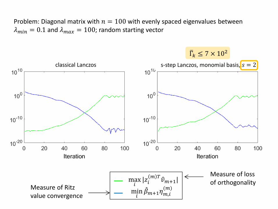
classical Lanczos s-step Lanczos, monomial basis, 𝑠 = 2
Γ𝑘 ≤ 7 × 10²
Measure of loss of orthogonality
Measure of Ritz value convergence
Problem: Diagonal matrix with 𝑛 = 100 with evenly spaced eigenvalues between 𝜆𝑚𝑖𝑛 = 0.1 and 𝜆𝑚𝑎𝑥 = 100; random starting vector
max𝑖
|𝑧𝑖𝑚 𝑇
𝑣𝑚+1|
min𝑖
𝛽𝑚+1𝜂𝑚,𝑖(𝑚)
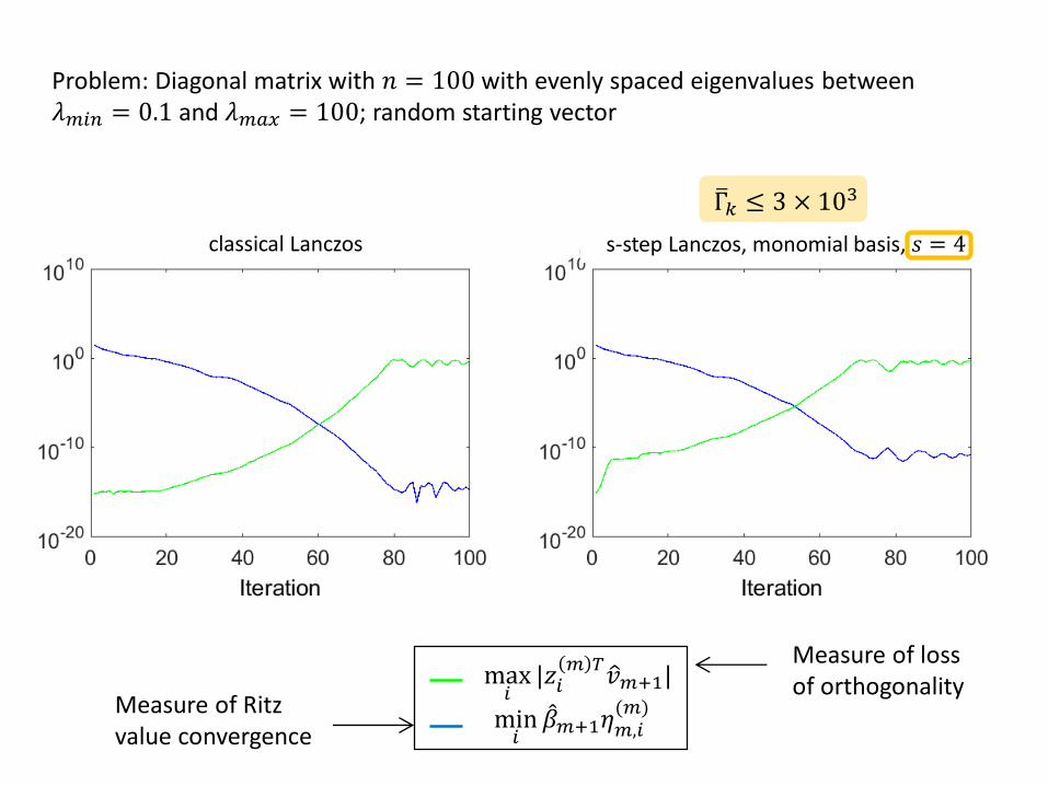
classical Lanczos s-step Lanczos, monomial basis, 𝑠 = 4
Γ𝑘 ≤ 3 × 10³
Measure of loss of orthogonality
Measure of Ritz value convergence

Problem: Diagonal matrix with 𝑛 = 100 with evenly spaced eigenvalues between 𝜆𝑚𝑖𝑛 = 0.1 and 𝜆𝑚𝑎𝑥 = 100; random starting vector
max𝑖
|𝑧𝑖𝑚 𝑇
𝑣𝑚+1|
min𝑖
𝛽𝑚+1𝜂𝑚,𝑖(𝑚)
classical Lanczos s-step Lanczos, monomial basis, 𝑠 = 8
Γ𝑘 ≤ 2 × 10⁶
Measure of loss of orthogonality
Measure of Ritz value convergence
Problem: Diagonal matrix with 𝑛 = 100 with evenly spaced eigenvalues between 𝜆𝑚𝑖𝑛 = 0.1 and 𝜆𝑚𝑎𝑥 = 100; random starting vector
max𝑖
|𝑧𝑖𝑚 𝑇
𝑣𝑚+1|
min𝑖
𝛽𝑚+1𝜂𝑚,𝑖(𝑚)
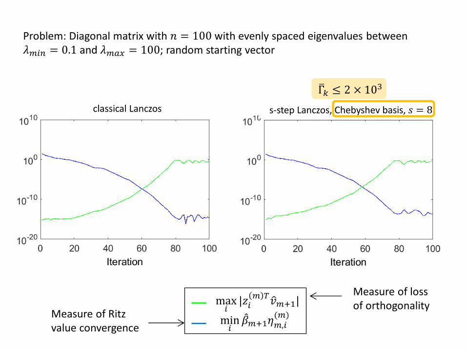
classical Lanczos s-step Lanczos, Chebyshev basis, 𝑠 = 8
Γ𝑘 ≤ 2 × 10³
Measure of loss of orthogonality
Measure of Ritz value convergence
Preconditioning for s-step variants• Preconditioners improve spectrum of system to improve convergence rate
• E.g., instead of 𝐴𝑥 = 𝑏, solve 𝑀−1𝐴𝑥 = 𝑀−1𝑏, where 𝑀−1 ≈ 𝐴−1
• Essential in practice
• In s-step variants, general preconditioning is a challenge
• Except for very simple cases, ability to exploit temporal locality across iterations is diminished by preconditioning
• If possible to avoid communication at all, usually necessitates significant modifications to the algorithm
• Tradeoff: speed up convergence, but increase time per iteration due to communication!
• For each specific app, must evaluate tradeoff between preconditioner quality and sparsity of the system
51

Recent efforts in s-step preconditioners• Much recent/ongoing work in developing communication-avoiding
preconditioned methods
• Many approaches shown to be compatible
• Diagonal
• Sparse Approx. Inverse (SAI) – same sparsity as 𝐴; recent work for CA-BICGSTAB by Mehri (2014)
• Polynomial preconditioning (Saad, 1985)
• HSS preconditioning (Hoemmen, 2010); for banded matrices (Knight, C., Demmel, 2014) - same general technique for any system that can be written as sparse + low-rank
• CA-ILU(0), CA-ILU(k) – Moufawad, Grigori (2013), Cayrols, Grigori (2015)
• Deflation for CA-CG (C., Knight, Demmel, 2014), based on Deflated CG of (Saad et al., 2000); for CA-GMRES (Yamazaki et al., 2014)
• Domain decomposition – avoid introducing additional communication by “underlapping” subdomains (Yamazaki, Rajamanickam, Boman, Hoemmen, Heroux, Tomov, 2014)
52

Summary• New communication-avoiding approaches to algorithm design are
necessary• But modifications may affect numerical properties
• s-step Krylov subspace methods can asymptotically reduce communication cost; potential applications in many scientific domains• But complicated tradeoffs depending on matrix structure,
numerical properties, and machine parameters
• Solving exascale-level problems efficiently will require a holisticapproach• Best method, best parameters, best preconditioners, etc. all very
problem- and machine-dependent• Requires a better understanding of how algorithmic changes affect
finite precision behavior
53