PERFORMANCE AND LOADS CORRELATION OF A UH-60A SLOWED ROTOR AT HIGH ADVANCE RATIOS

Sesi Kottapalli

Flight Vehicle Research and Technology Division NASA Ames Research Center

Moffett Field, California sesi.kottapalli@nasa.gov

Measured data from the slowed-rotor 2010 UH-60A Airloads Rotor test in the NASA Ames 40- by 80- Foot Wind Tunnel are compared with CAMRAD II calculations. The emphasis is to correlate overall trends. This analytical effort considers advance ratios from 0.3 to 1.0, with the rotor rotational speed at 40%NR. The rotor performance parameters considered are the thrust coefficient, power coefficient, L/DE, torque, and H-force. The blade loads considered are the half peak-to-peak, mid-span and outboard torsion, flatwise, and chordwise moments, and the pitch link load. For advance ratios ≤ 0.7, the overall trends for the performance and loads (excluding the pitch link load) could be captured, but with substantial overprediction or underprediction. The correlation gradually deteriorates as the advance ratio is increased and for advance ratios ≥ 0.8 there is no correlation. The pitch link load correlation is not good. There is considerable scope for improvement in the prediction of the blade loads. Considering the modeling complexity associated with the unconventional operating condition under consideration, the current predictive ability to capture overall trends is encouraging.

Notation CH Rotor H-force coefficient CL Rotor lift coefficient CP Rotor power coefficient CQ Rotor torque coefficient CT Rotor thrust coefficient H-force Rotor drag in shaft axes, lb L/DE Rotor lift to effective drag ratio NP Integer (N) multiple of rotor speed R Rotor radius, ft V Forward speed, ft/sec %NR % of normal rotor rotational speed αs Rotor shaft angle, deg µ Rotor advance ratio (V/ΩR) σ Rotor solidity ratio Ω Rotor rotational speed, rad/sec

Introduction In 2010, NASA and the U.S. Army completed a full-scale wind tunnel test of the heavily instrumented UH-60A Airloads Rotor, Ref. 1. During this test, in addition to normal advance ratio flight conditions, high advance ratio conditions were also explored and experimental data acquired at advance ratios up to µ = 1.0. To increase the advance ratio, the UH-60A rotor RPM was slowed down to as low as 40%NR (data were also acquired at 65%NR). In the current study, the measured high advance ratio performance and rotor loads data at 40%NR are compared _______________________________ Presented at the American Helicopter Society Future Vertical Lift Aircraft Design Conference, January 18-20, 2012, San Francisco, California. This is a work of the U.S. Government and is not subject to copyright protection in the U.S.

with analytical predictions. This effort is currently a work in progress. In 2008, the experimental and theoretical performances of three different rotors, excluding the UH-60A, were studied using five analyses, Ref. 2. Recently, the 2010 UH-60A test data were carefully studied to obtain a fundamental understanding of the various physical phenomena associated with the high advance ratio operating condition, Ref. 3. The emphasis in this initial study is on correlating overall trends. Since the slowed rotor condition is an unconventional operating condition, the paper includes both dimensional and non-dimensional comparisons of the measurements and predictions. An eventual goal is to identify the limits of comprehensive analyses, and assess whether the current aerodynamic representations of large regions of reverse flow, etc. are sufficiently appropriate or if computational fluid dynamics, CFD, is needed. Overall, the paper includes rotor performance correlations of the type shown in Ref. 2. This enables an assessment of the correlation level currently achievable for the UH-60A using comprehensive analyses relative to the Ref. 2 correlation level. The present study considers the first step in the prediction of the reduced RPM UH-60A performance and rotor loads. A fixed, rigid hub is considered, i.e. the effects of the wind tunnel test stand, the Large Rotor Test Apparatus, LRTA, are not included. The rotorcraft comprehensive analysis CAMRAD II, Refs. 4-6, is used to produce analytical predictions. The most recent UH-60A CAMRAD II rotor model is used in this study, Ref. 7.

Measured Wind Tunnel Data Reference 1 contains a description of the UH-60A slowed

2

rotor testing conducted in the National Full-Scale Aerodynamics Complex (NFAC) 40- by 80-Foot Wind Tunnel.

Analytical Model

The CAMRAD II model used is briefly described as follows. The model includes an elastic blade. The UH-60A rotor blade is modeled using elastic beam elements, with each element having two elastic flap bending, two elastic lag bending, and two torsion degrees of freedom. The blade consists of four beam elements. For the rotor trim procedure, 12 blade modes are used. The analytical trim procedure is similar to the wind tunnel test trim procedure for high advance ratio slowed rotors, i.e., given an advance ratio and collective pitch, the lateral and longitudinal cyclics are adjusted to minimize the blade 1P flapping. At higher advance ratios it became necessary to relax the flapping tolerance in order to get converged results. The prescribed (rigid) wake model is used. At present, the UH-60A control system stiffness is based on the flight test article, Ref. 7. Any differences associated with the current wind tunnel configuration have not been accounted for in this study.

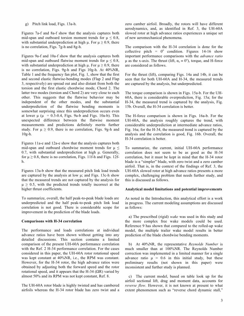
Results Correlations of the performance and loads for µ = 0.3 to 1.0 at a rotor rotational speed 40%NR (approximately 104 RPM) and shaft angle αs = 0o are shown in this paper. Figure 1 shows the calculated frequency fan plot for the UH-60A rotor. At 40%NR, the first elastic chordwise mode (“Chord 2” in the figure) and the torsion mode are close to each other, in the range 10P -12P, Table 1. In the correlation figures that follow, the predictions are shown in solid blue lines and the measurements are shown in solid red lines. Also, for each correlation parameter, the vertical axis scale is kept the same at all advance ratios for easier comparison. Rotor performance Figures 2-6 show the performance correlations for µ = 0.3 to 1.0, listed as follows: a) Thrust coefficient CT/σ versus collective, Figs. 2a-h. b) Power coefficient CP/σ versus CT/σ, Figs. 3a-h c) Rotor lift to effective drag L/DE versus CL/σ, Figs. 4a-h d) Torque versus CT/σ, Figs. 5a-h e) H-force versus CT/σ, Figs. 6a-h. For the thrust coefficient CT/σ, Figs. 2a-g show that both test and analysis have roughly the same linear trend with collective. However, the analysis underpredicts CT/σ, and at high µ (µ = 0.7, Fig. 2e), this results in an equivalent discrepancy (delta) of 2o in the collective pitch. It appears that the slope of CT/σ with respect to the collective decreases

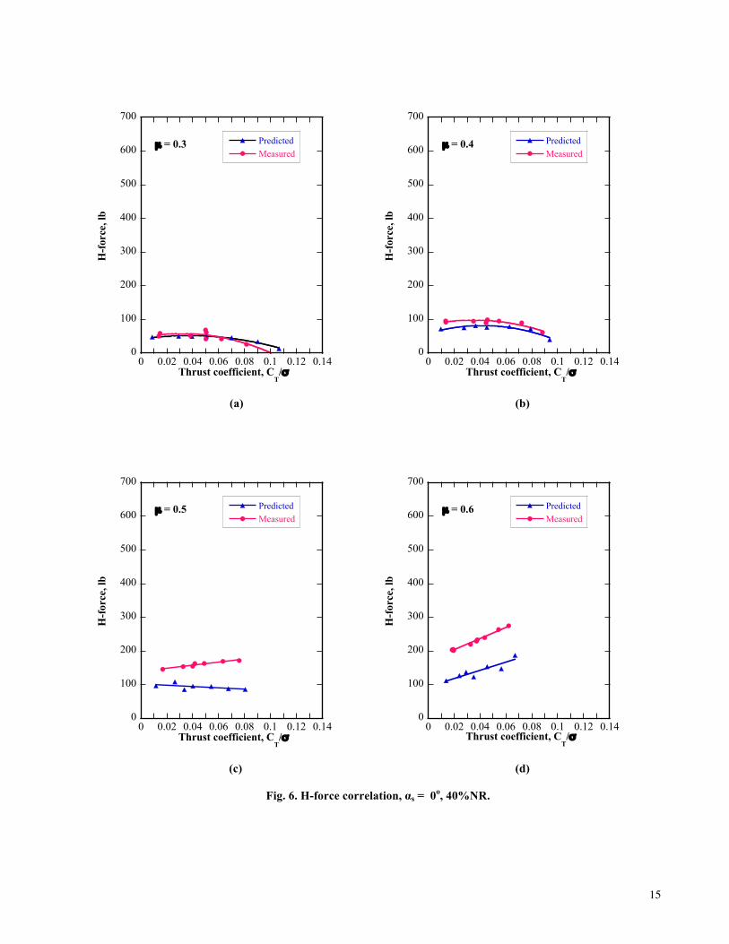
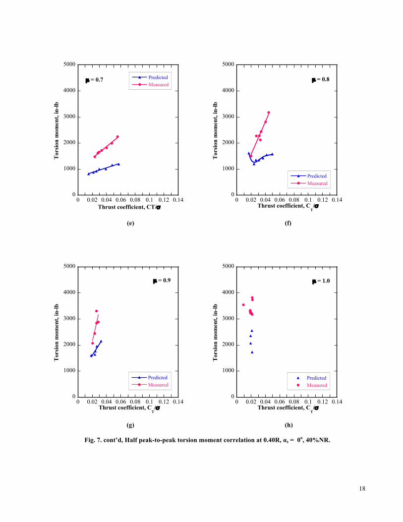
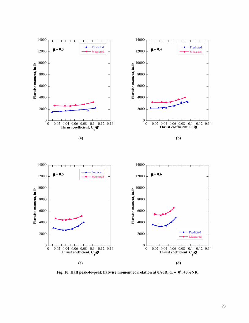
as the advance ratio is increased. Also, at µ = 1.0, Fig. 2h, the thrust coefficient CT/σ has a very small value, approximately 0.02 and is independent of the collective. Figures 3a-e show that the analysis captures the measured power coefficient CP/σ nonlinear trend with CT/σ for µ ≤ 0.7, with substantial overprediction at high µ. For µ ≥ 0.8, there is no correlation, Figs. 3f-h. Figures 4a-e show that the analysis captures the measured rotor L/DE trends for µ ≤ 0.7, with substantial overprediction at high µ. For µ ≥ 0.8, there is no correlation, Figs. 4f-h. For the CT/σ range under consideration, approximately 0.01 to 0.11, the L/DE ratio goes from ≤ 2 to ≥8, Figs. 4a-h. The effective drag DE depends on the accurate determination of both the profile and induced drag contributions, thus complicating the prediction of L/DE. This merits further study since the accurate prediction of L/DE is extremely important in the estimation of aircraft range. Figures 5a-c show that the dimensional rotor torque is well predicted at low µ for this low rotor speed, 104 RPM, condition. As expected, the torque and the power coefficient, Figs. 5a-e and 3a-e, have similar trends, i.e., nonlinear increase with CT/σ, and similar to the power coefficient correlation, the analysis captures the measured rotor torque trends for µ ≤ 0.7, Figs. 5a-e, with substantial overprediction at high µ. For µ ≥ 0.8, there is no correlation, Figs. 5f-h. Figures 6a-g show that the analysis captures the measured H-force trends for µ ≤ 0.9, with substantial underprediction at high µ. For µ = 1.0, there is no correlation, Fig. 6h. Both test and analysis show the same linear trend at high µ, µ = 0.6-0.9, Figs. 6d-g. The H-force, the rotor drag in the shaft axes, generally increases with the advance ratio, Figs. 6a-h. Blade loads and pitch link load In order to expeditiously assess the overall predictive capability of the current analytical model, only half peak-to-peak loads are considered in this initial study. Azimuthal time histories may be considered in a more detailed, anticipated follow-on study that would most likely focus on specific, limited combinations of µ and CT/σ. Figures 7-12 show the half peak-to-peak torsion, flatwise and chordwise blade moments at the mid-span and outboard stations, and Fig. 13 shows the half peak-to-peak pitch link load, all as a function of the thrust coefficient CT/σ. The measured half peak-to-peak loads were obtained from averaged time-histories. These correlations, for µ = 0.3 to 1.0, are listed as follows: a) Torsion moment at 0.40C, Figs. 7a-h b) Torsion moment at 0.80C, Figs. 8a-h c) Flatwise bending moment at 0.50C, Figs. 9a-h d) Flatwise bending moment at 0.80C, Figs. 10a-h e) Chordwise bending moment at 0.40C, Figs. 11a-h f) Chordwise bending moment at 0.80C, Figs. 12a-h

3

g) Pitch link load, Figs. 13a-h. Figures 7a-f and 8a-f show that the analysis captures both mid-span and outboard torsion moment trends for µ ≤ 0.8, with substantial underprediction at high µ. For µ ≥ 0.9, there is no correlation, Figs. 7g-h and 8g-h. Figures 9a-f and 10a-f show that the analysis captures both mid-span and outboard flatwise moment trends for µ ≤ 0.8, with substantial underprediction at high µ. For µ ≥ 0.9, there is no correlation, Figs. 9g-h and Figs 10g-h. At 40%NR, Table 1 and the frequency fan plot, Fig. 1, show that the first and second elastic flatwise-bending modes (Flap 2 and Flap 3, respectively) are spread out and also distant from both the torsion and the first elastic chordwise mode, Chord 2. The latter two modes (torsion and Chord 2) are very close to each other. This suggests that the flatwise behavior may be independent of the other modes, and the substantial underprediction of the flatwise bending moments is somewhat surprising since this underprediction occurs even at lower µ (µ = 0.3-0.4, Figs. 9a-b and Figs. 10a-b). This unexpected difference between the flatwise moment measurements and predictions definitely merits further study. For µ ≥ 0.9, there is no correlation, Figs. 9g-h and 10g-h. Figures 11a-e and 12a-e show that the analysis captures both mid-span and outboard chordwise moment trends for µ ≤ 0.7, with substantial underprediction at high µ. Generally, for µ ≥ 0.8, there is no correlation, Figs. 11f-h and Figs. 12f-h. Figures 13a-b show that the measured pitch link load trends are captured by the analysis at low µ; and Figs. 13c-h show that the measured trends are not captured by the analysis for µ ≥ 0.5, with the predicted trends totally incorrect at the higher thrust coefficients. To summarize, overall, the half peak-to-peak blade loads are underpredicted and the half peak-to-peak pitch link load correlation is not good. There is considerable scope for improvement in the prediction of the blade loads. Comparisons with H-34 correlation The performance and loads correlations at individual advance ratios have been shown without getting into any detailed discussions. This section contains a limited comparison of the present UH-60A performance correlation with the Ref. 2 H-34 performance correlation. For the cases considered in this paper, the UH-60A rotor rotational speed was kept constant at 40%NR, i.e., the RPM was constant. However, for the H-34 rotor, the high advance ratios were obtained by adjusting both the forward speed and the rotor rotational speed, and it appears that the H-34 (ΩR) varied by almost 50% and its RPM was not kept constant, Ref. 8. The UH-60A rotor blade is highly twisted and has cambered airfoils whereas the H-34 rotor blade has zero twist and a

zero camber airfoil. Broadly, the rotors will have different aerodynamics, and, as identified in Ref. 3, the UH-60A slowed rotor at high advance ratios experiences a unique set of new aeromechanical phenomena. The comparison with the H-34 correlation is done for the collective pitch = 0o condition. Figures 14-16 show important performance comparisons with the advance ratio µ as the x-axis. The thrust (lift, αs = 0o), torque, and H-force are considered as follows. For the thrust (lift), comparing Figs. 14a and 14b, it can be seen that for both UH-60A and H-34, the measured trends are captured by the analysis, but underpredicted. The torque comparison is shown in Figs. 15a-b. For the UH-60A, there is considerable overprediction, Fig. 15a; for the H-34, the measured trend is captured by the analysis, Fig. 15b. Overall, the H-34 correlation is better. The H-force comparison is shown in Figs. 16a-b. For the UH-60A, the analysis roughly captures the trend, with considerable underprediction at intermediate advance ratios, Fig. 16a; for the H-34, the measured trend is captured by the analysis and the correlation is good, Fig. 16b. Overall, the H-34 correlation is better. To summarize, the current, initial UH-60A performance correlation does not seem to be as good as the H-34 correlation, but it must be kept in mind that the H-34 rotor blade is a “simpler” blade, with zero twist and a zero camber airfoil. That is, in the context of the findings of Ref. 3, the UH-60A slowed rotor at high advance ratios presents a more complex, challenging problem that needs further study, and this is discussed as follows. Analytical model limitations and potential improvements As noted in the Introduction, this analytical effort is a work in progress. The current modeling assumptions are discussed as follows: a) The prescribed (rigid) wake was used in this study and the more complex free wake models could be used. Reference 9 has shown that compared to the rolled-up wake model, the multiple trailer wake model results in better prediction of the blade chordwise bending moments. b) At 40%NR, the representative Reynolds Number is much smaller than at 100%NR. The Reynolds Number correction was implemented in a limited manner for a single advance ratio µ = 0.6 in this initial study, but these preliminary results (not shown in this paper) were inconsistent and further study is planned. c) The current model, based on table look up for the airfoil sectional lift, drag and moment data, accounts for reverse flow. However, it is not known at present to what extent phenomenon such as “reverse chord dynamic stall,”

4

Ref. 3, would modify the current UH-60A airfoil tables (that is, without getting into CFD-based computing). Semi-empirical modifications to the airfoil tables may be one approach that can be pursued. Such modifications have been successfully implemented in Ref. 9 for a different rotor system. d) As noted in the Analytical Model section, the currently used UH-60A control system stiffness is based on the flight test article and any differences in the control system stiffness associated with the current wind tunnel configuration have not been accounted for in this study. Considering that the current pitch link load correlation is not good and could be improved, the analytical control system model should be considered in more detail for possible revision. Finally, plotting both measured and predicted data versus the collective, or µ, instead of CT/σ will give different insight. At high µ, CT/σ does not change much with collective so the data tends to go straight up. An anticipated follow-on study will implement this suggestion, but before this is done, the discrepancy noted in the discussion of Fig. 2, the delta between the experimental and analytical collectives, has to be resolved. Perhaps, the advance ratio µ could be used as the independent parameter, the x-axis, e.g., Fig. 14.

Conclusions The prediction of UH-60A rotor performance and loads at high advance ratio was considered in this analytical study. Measured data from the 40- by 80-Foot Wind Tunnel were compared with CAMRAD II predictions. The emphasis in this initial study was to correlate overall trends. Initial results that represent work in progress were shown and found to be encouraging. For a rotor rotational speed 40%NR (approximately 104 RPM) and shaft angle αs = 0o, the complete range of advance ratios, µ = 0.3-1.0, was considered The rotor performance parameters considered were as follows: thrust coefficient, power coefficient, L/DE, torque, and H-force. The blade loads considered were as follows: the half peak-to-peak mid-span and outboard torsion, flatwise, and chordwise moments, and the pitch link load. It was found that for advance ratios ≤ 0.7, the overall trends for the performance and loads (excluding the pitch link load) could be captured, but with substantial overprediction or underprediction. The correlation gradually deteriorated as the advance ratio was increased and for advance ratios ≥ 0.8 there was no correlation. The pitch link load correlation was not good. There is considerable scope for improvement in the prediction of the blade loads. The limitations of the current analytical model and potential improvements to the model were discussed, for possible implementation in a follow-on study. Considering the modeling complexity associated with the unconventional

operating condition under consideration, it is believed that the current predictive ability to capture overall trends is encouraging.

References 1. Norman, T. R., Shinoda, P., Peterson, R. L., and Datta, A., “Full-Scale Wind Tunnel Test of The UH-60A Airloads Rotor,” American Helicopter Society Annual Forum 67, May 3-5, Virginia Beach, VA, 2011. 2. Harris, F. D., “Rotor Performance at High Advance Ratio; Theory versus Test,” NASA CR 2008-215370, October 2008. 3. Datta, A., Yeo, H., and Norman, T. R., “Experimental Investigation and Fundamental Understanding of a Slowed UH-60A Rotor at High Advance Ratios,” American Helicopter Society 67th Annual Forum, Virginia Beach, VA, May 2011. 4. Johnson, W. "CAMRAD II, Comprehensive Analytical Model of Rotorcraft Aerodynamics and Dynamics," Johnson Aeronautics, Palo Alto, California, 1992-1999. 5. Johnson, W. "Technology Drivers in the Development of CAMRAD II," American Helicopter Society, American Helicopter Society Aeromechanics Specialists Conference, San Francisco, CA, January 19-21, 1994. 6. Johnson, W. "A General Free Wake Geometry Calculation for Wings and Rotors,” American Helicopter Society 51st Annual Forum Proceedings, Ft. Worth, TX, May 9-11, 1995. 7. Yeo, H., Bousman, W.G., and Johnson, W., “Performance Analysis of a Utility Helicopter with Standard and Advanced Rotor,” Journal of the American Helicopter Society, Vol. 49, No. 3, July 2004, pp. 250–270. 8. McCloud III, John L., Biggers, James C., and Stroub, R.H, “An Investigation of Full-Scale Helicopter Rotors at High Advance Ratios and Advancing Tip Mach Numbers,” NASA TN D-4632, 1968. 9. Kottapalli, S. “Enhanced Correlation of SMART Active Flap Rotor Loads,” American Institute of Aeronautics and Astronautics 52nd AIAA/ASME/ASCE/AHS/ASC Structures, Structural Dynamics, and Materials Conference, Denver, CO, April 4-7, 2011, AIAA 2011-1874.

5

Table 1. Calculated UH-60A rotor blade frequencies, 40%NR.

__________________________________________ _________________________________________________________________________________________________________

Blade Mode Frequency (per rev) ___________________________________

Chord 1 0.32

Flap 1 1.05 Flap 2 3.32

Flap 3 7.33 Chord 2 10.58 Torsion 1 11.20

__________________________________________________________________________________________________________ __________________________________________________________________________________________________________

6

Fig. 1. UH-60A rotor fan plot.

0

5

10

15

20

25

0 0.1 0.2 0.3 0.4 0.5 0.6 0.7 0.8 0.9 1 1.1 1.2

Freq

uenc

y, H

z

Normalized Rotor Speed

1P

2P

3P

4P

5P

Chord 1

Flap 1

Flap 2

Torsion 1

Chord 2

Flap 3

6P 7P 8P 12P

7

(a) (b)

(c) (d)

Fig. 2. Thrust coefficient correlation, αs = 0o, 40%NR.

0.00

0.02

0.04

0.06

0.08

0.10

0.12

-2 0 2 4 6 8 10 12

PredictedMeasured

Thr

ust c

oeff

icie

nt, C

T/ !

Collective, deg

µ = 0.3

0.00

0.02

0.04

0.06

0.08

0.10

0.12

-2 0 2 4 6 8 10 12

PredictedMeasured

Thr

ust c

oeff

icie

nt, C

T/ !

Collective, deg

µ = 0.4

0.00

0.02

0.04

0.06

0.08

0.10

0.12

-2 0 2 4 6 8 10 12

PredictedMeasured

Thr

ust c

oeff

icie

nt, C

T/ !

Collective, deg

µ = 0.5

0.00

0.02

0.04

0.06

0.08

0.10

0.12

-2 0 2 4 6 8 10 12

PredictedMeasured

Thr

ust c

oeff

icie

nt, C

T/!

Collective, deg

µ = 0.6

8

(e) (f)

(g) (h)

Fig. 2. cont’d, Thrust coefficient correlation, αs = 0o, 40%NR.

0.00

0.02

0.04

0.06

0.08

0.10

0.12

-2 0 2 4 6 8 10 12

PredictedMeasured

Thr

ust c

oeff

icie

nt, C

T/!

Collective, deg

µ = 0.7

0.00

0.02

0.04

0.06

0.08

0.10

0.12

-2 0 2 4 6 8 10 12

PredictedMeasured

Thr

ust c

oeff

icie

nt, C

T/ !

Collective, deg

µ = 0.8

0.00

0.02

0.04

0.06

0.08

0.10

0.12

-2 0 2 4 6 8 10 12

PredictedMeasured

Thr

ust c

oeff

icie

nt, C

T/!

Collective, deg

µ = 0.9

0.00

0.02

0.04

0.06

0.08

0.10

0.12

-2 0 2 4 6 8 10 12

PredictedMeasured

Thr

ust c

oeff

icie

nt, C

T/ !

Collective, deg

µ = 1.0

9

(a) (b)

(c) (d)

Fig. 3. Power coefficient correlation, αs = 0o, 40%NR.

0.000

0.001

0.002

0.003

0.004

0.005

0.006

0 0.02 0.04 0.06 0.08 0.1 0.12 0.14

PredictedMeasured

Pow

er c

oeff

icie

nt, C

P/!

Thrust coefficient, CT/!

µ = 0.3

0.000

0.001

0.002

0.003

0.004

0.005

0.006

0 0.02 0.04 0.06 0.08 0.1 0.12 0.14

PredictedMeasured

Pow

er c

oeff

icie

nt, C

P/ !Thrust coefficient, C

T/!

µ = 0.4

0.000

0.001

0.002

0.003

0.004

0.005

0.006

0 0.02 0.04 0.06 0.08 0.1 0.12 0.14

PredictedMeasured

Pow

er c

oeff

icie

nt, C

P/ !

Thrust coefficient, CT/!

µ = 0.5

0.000

0.001

0.002

0.003

0.004

0.005

0.006

0 0.02 0.04 0.06 0.08 0.1 0.12 0.14

PredictedMeasured

Pow

er c

oeff

icie

nt, C

P/!

Thrust coefficient, CT/!

µ = 0.6

10

(e) (f)

(g) (h)

Fig. 3. cont’d, Power coefficient correlation, αs = 0o, 40%NR.

0.000

0.001

0.002

0.003

0.004

0.005

0.006

0 0.02 0.04 0.06 0.08 0.1 0.12 0.14

PredictedMeasured

Pow

er c

oeff

icie

nt, C

P/ !

Thrust coefficient, CT/!

µ = 0.7

0.000

0.001

0.002

0.003

0.004

0.005

0.006

0 0.02 0.04 0.06 0.08 0.1 0.12 0.14

PredictedMeasured

Pow

er c

oeff

icie

nt, C

P/!Thrust coefficient, C

T/!

µ = 0.8

0.000

0.001

0.002

0.003

0.004

0.005

0.006

0 0.02 0.04 0.06 0.08 0.1 0.12 0.14

PredictedMeasured

Pow

er c

oeff

icie

nt, C

P/ !

Thrust coefficient, CT/!

µ = 0.9

0.000

0.001

0.002

0.003

0.004

0.005

0.006

0 0.02 0.04 0.06 0.08 0.1 0.12 0.14

PredictedMeasured

Pow

er c

oeff

icie

nt, C

P/!

Thrust coefficient, CT/!

µ = 1.0

11

(a) (b)

(c) (d)

Fig. 4. Lift to drag ratio correlation, αs = 0o, 40%NR.

0

2

4

6

8

10

0 0.02 0.04 0.06 0.08 0.1 0.12

PredictedMeasured

Lift

to d

rag

ratio

, L/D

E

Lift coefficient, CL/!

µ = 0.3

0

2

4

6

8

10

0 0.02 0.04 0.06 0.08 0.1 0.12

PredictedMeasured

Lift

to d

rag

ratio

, L/D

E

Lift coefficient, CL/!

µ = 0.4

0

2

4

6

8

10

0 0.02 0.04 0.06 0.08 0.1 0.12

PredictedMeasured

Lift

to d

rag

ratio

, L/D

E

Lift coefficient, CL/!

µ = 0.5

0

2

4

6

8

10

0 0.02 0.04 0.06 0.08 0.1 0.12

PredictedMeasured

Lift

to d

rag

ratio

, L/D

E

Lift coefficient, CL/!

µ = 0.6

12

(e) (f)

(g) (h)

Fig. 4. cont’d, Lift to drag ratio correlation, αs = 0o, 40%NR.

0

2

4

6

8

10

0 0.02 0.04 0.06 0.08 0.1 0.12

PredictedMeasured

Lift

to d

rag

ratio

, L/D

E

Lift coefficient, CL/!

µ = 0.7

0

2

4

6

8

10

0 0.02 0.04 0.06 0.08 0.1 0.12

PredictedMeasured

Lift

to d

rag

ratio

, L/D

E

Lift coefficient, CL/!

µ = 0.8

0

2

4

6

8

10

0 0.02 0.04 0.06 0.08 0.1 0.12

PredictedMeasured

Lift

to d

rag

ratio

, L/D

E

Lift coefficient, CL/!

µ = 0.9

0

2

4

6

8

10

0 0.02 0.04 0.06 0.08 0.1 0.12

PredictedMeasured

Lift

to d

rag

ratio

, L/D

E

Lift coefficient, CL/!

µ = 1.0

13

(a) (b)

(c) (d)

Fig. 5. Rotor torque correlation, αs = 0o, 40%NR.

0

1000

2000

3000

4000

5000

0 0.02 0.04 0.06 0.08 0.1 0.12 0.14

PredictedMeasured

Rot

or to

rque

, ft-

lb

Thrust coefficient, CT/!

µ = 0.3

0

1000

2000

3000

4000

5000

0 0.02 0.04 0.06 0.08 0.1 0.12 0.14

PredictedMeasured

Rot

or to

rque

, ft-

lbThrust coefficient, C

T/!

µ = 0.4

0

1000

2000

3000

4000

5000

0 0.02 0.04 0.06 0.08 0.1 0.12 0.14

PredictedMeasured

Rot

or to

rque

, ft-

lb

Thrust coefficient, CT/!

µ = 0.5

0

1000

2000

3000

4000

5000

0 0.02 0.04 0.06 0.08 0.1 0.12 0.14

PredictedMeasured

Rot

or to

rque

, ft-

lb

Thrust coefficient, CT/!

µ = 0.6

14

(e) (f)

(g) (h)

Fig. 5. cont’d, Rotor torque correlation, αs = 0o, 40%NR.

0

1000

2000

3000

4000

5000

0 0.02 0.04 0.06 0.08 0.1 0.12 0.14

PredictedMeasured

Rot

or to

rque

, ft-

lb

Thrust coefficient, CT/!

µ = 0.7

0

1000

2000

3000

4000

5000

0 0.02 0.04 0.06 0.08 0.1 0.12 0.14

PredictedMeasured

Rot

or to

rque

, ft-

lbThrust coefficient, C

T/!

µ = 0.8

0

1000

2000

3000

4000

5000

0 0.02 0.04 0.06 0.08 0.1 0.12 0.14

PredictedMeasured

Rot

or to

rque

, ft-

lb

Thrust coefficient, CT/!

µ = 0.9

0

1000

2000

3000

4000

5000

0 0.02 0.04 0.06 0.08 0.1 0.12 0.14

PredictedMeasured

Rot

or to

rque

, ft-

lb

Thrust coefficient, CT/!

µ = 1.0

15

(a) (b)

(c) (d)

Fig. 6. H-force correlation, αs = 0o, 40%NR.

0

100

200

300

400

500

600

700

0 0.02 0.04 0.06 0.08 0.1 0.12 0.14

PredictedMeasured

H-f

orce

, lb

Thrust coefficient, CT/!

µ = 0.3

0

100

200

300

400

500

600

700

0 0.02 0.04 0.06 0.08 0.1 0.12 0.14

PredictedMeasured

H-f

orce

, lb

Thrust coefficient, CT/!

µ = 0.4

0

100

200

300

400

500

600

700

0 0.02 0.04 0.06 0.08 0.1 0.12 0.14

PredictedMeasured

H-f

orce

, lb

Thrust coefficient, CT/!

µ = 0.5

0

100

200

300

400

500

600

700

0 0.02 0.04 0.06 0.08 0.1 0.12 0.14

PredictedMeasured

H-f

orce

, lb

Thrust coefficient, CT/!

µ = 0.6

16

(e) (f)

(g) (h)

Fig. 6. cont’d, H-force correlation, αs = 0o, 40%NR.

0

100

200

300

400

500

600

700

0 0.02 0.04 0.06 0.08 0.1 0.12 0.14

PredictedMeasured

H-f

orce

, lb

Thrust coefficient, CT/!

µ = 0.7

0

100

200

300

400

500

600

700

0 0.02 0.04 0.06 0.08 0.1 0.12 0.14

PredictedMeasured

H-f

orce

, lb

Thrust coefficient, CT/!

µ = 0.8

0

100

200

300

400

500

600

700

0 0.02 0.04 0.06 0.08 0.1 0.12 0.14

PredictedMeasured

H-f

orce

, lb

Thrust coefficient, CT/!

µ = 0.9

0

100

200

300

400

500

600

700

0 0.02 0.04 0.06 0.08 0.1 0.12 0.14

PredictedMeasured

H-f

orce

, lb

Thrust coefficient, CT/!

µ = 1.0

17

(a) (b)

(c) (d)

Fig. 7. Half peak-to-peak torsion moment correlation at 0.40R, αs = 0o, 40%NR.

0

1000

2000

3000

4000

5000

0 0.02 0.04 0.06 0.08 0.1 0.12 0.14

PredictedMeasured

Tor

sion

mom

ent,

in-lb

Thrust coefficient, CT/!

µ = 0.3

0

1000

2000

3000

4000

5000

0 0.02 0.04 0.06 0.08 0.1 0.12 0.14

PredictedMeasured

Tor

sion

mom

ent,

in-lb

Thrust coefficient, CT/!

µ = 0.4

0

1000

2000

3000

4000

5000

0 0.02 0.04 0.06 0.08 0.1 0.12 0.14

PredictedMeasured

Tor

sion

mom

ent,

in-lb

Thrust coefficient, CT/!

µ = 0.5

0

1000

2000

3000

4000

5000

0 0.02 0.04 0.06 0.08 0.1 0.12 0.14

PredictedMeasured

Tor

sion

mom

ent,

in-lb

Thrust coefficient, CT/!

µ = 0.6

18

(e) (f)

(g) (h)

Fig. 7. cont’d, Half peak-to-peak torsion moment correlation at 0.40R, αs = 0o, 40%NR.

0

1000

2000

3000

4000

5000

0 0.02 0.04 0.06 0.08 0.1 0.12 0.14

PredictedMeasured

Tor

sion

mom

ent,

in-lb

Thrust coefficient, CT/!

µ = 0.7

0

1000

2000

3000

4000

5000

0 0.02 0.04 0.06 0.08 0.1 0.12 0.14

PredictedMeasured

Tor

sion

mom

ent,

in-lb

Thrust coefficient, CT/!

µ = 0.8

0

1000

2000

3000

4000

5000

0 0.02 0.04 0.06 0.08 0.1 0.12 0.14

PredictedMeasured

Tor

sion

mom

ent,

in-lb

Thrust coefficient, CT/!

µ = 0.9

0

1000

2000

3000

4000

5000

0 0.02 0.04 0.06 0.08 0.1 0.12 0.14

PredictedMeasured

Tor

sion

mom

ent,

in-lb

Thrust coefficient, CT/!

µ = 1.0

19

(a) (b)

(c) (d)

Fig. 8. Half peak-to-peak torsion moment correlation at 0.80R, αs = 0o, 40%NR.

0

200

400

600

800

1000

0 0.02 0.04 0.06 0.08 0.1 0.12 0.14

PredictedMeasured

Tor

sion

mom

ent,

in-lb

Thrust coefficient, CT/!

µ = 0.3

0

200

400

600

800

1000

0 0.02 0.04 0.06 0.08 0.1 0.12 0.14

PredictedMeasured

Tor

sion

mom

ent,

in-lb

Thrust coefficient, CT/!

µ = 0.4

0

200

400

600

800

1000

0 0.02 0.04 0.06 0.08 0.1 0.12 0.14

PredictedMeasured

Tor

sion

mom

ent,

in-lb

Thrust coefficient, CT/!

µ = 0.5

0

200

400

600

800

1000

0 0.02 0.04 0.06 0.08 0.1 0.12 0.14

PredictedMeasured

Tor

sion

mom

ent,

in-lb

Thrust coefficient, CT/!

µ = 0.6

20

(e) (f)

(g) (h)

Fig. 8. cont’d, Half peak-to-peak torsion moment correlation at 0.80R, αs = 0o, 40%NR.

0

200

400

600

800

1000

0 0.02 0.04 0.06 0.08 0.1 0.12 0.14

PredictedMeasured

Tor

sion

mom

ent,

in-lb

Thrust coefficient, CT/!

µ = 0.7

0

200

400

600

800

1000

0 0.02 0.04 0.06 0.08 0.1 0.12 0.14

PredictedMeasured

Tor

sion

mom

ent,

in-lb

Thrust coefficient, CT/!

µ = 0.8

0

200

400

600

800

1000

0 0.02 0.04 0.06 0.08 0.1 0.12 0.14

PredictedMeasured

Tor

sion

mom

ent,

in-lb

Thrust coefficient, CT/!

µ = 0.9

0

200

400

600

800

1000

0 0.02 0.04 0.06 0.08 0.1 0.12 0.14

PredictedMeasured

Tor

sion

mom

ent,

in-lb

Thrust coefficient, CT/!

µ = 1.0

21

(a) (b)

(c) (d)

Fig. 9. Half peak-to-peak flatwise moment correlation at 0.50R, αs = 0o, 40%NR.

0

4000

8000

12000

16000

20000

24000

28000

32000

0 0.02 0.04 0.06 0.08 0.1 0.12 0.14

PredictedMeasured

Flat

wis

e m

omen

t, in

-lb

Thrust coefficient, CT/!

µ = 0.3

0

4000

8000

12000

16000

20000

24000

28000

32000

0 0.02 0.04 0.06 0.08 0.1 0.12 0.14

PredictedMeasured

Flat

wis

e m

omen

t, in

-lbThrust coefficient, C

T/!

µ = 0.4

0

4000

8000

12000

16000

20000

24000

28000

32000

0 0.02 0.04 0.06 0.08 0.1 0.12 0.14

PredictedMeasured

Flat

wis

e m

omen

t, in

-lb

Thrust coefficient, CT/!

µ = 0.5

0

4000

8000

12000

16000

20000

24000

28000

32000

0 0.02 0.04 0.06 0.08 0.1 0.12 0.14

PredictedMeasured

Flat

wis

e m

omen

t, in

-lb

Thrust coefficient, CT/!

µ = 0.6

22

(e) (f)

(g) (h)

Fig. 9. cont’d, Half peak-to-peak flatwise moment correlation at 0.50R, αs = 0o, 40%NR.

0

4000

8000

12000

16000

20000

24000

28000

32000

0 0.02 0.04 0.06 0.08 0.1 0.12 0.14

PredictedMeasured

Flat

wis

e m

omen

t, in

-lb

Thrust coefficient, CT/!

µ = 0.7

0

4000

8000

12000

16000

20000

24000

28000

32000

0 0.02 0.04 0.06 0.08 0.1 0.12 0.14

PredictedMeasured

Flat

wis

e m

omen

t, in

-lbThrust coefficient, C

T/!

µ = 0.8

0

4000

8000

12000

16000

20000

24000

28000

32000

0 0.02 0.04 0.06 0.08 0.1 0.12 0.14

PredictedMeasured

Flat

wis

e m

omen

t, in

-lb

Thrust coefficient, CT/!

µ = 0.9

0

4000

8000

12000

16000

20000

24000

28000

32000

0 0.02 0.04 0.06 0.08 0.1 0.12 0.14

PredictedMeasured

Flat

wis

e m

omen

t, in

-lb

Thrust coefficient, CT/!

µ = 1.0

23

(a) (b)

(c) (d)

Fig. 10. Half peak-to-peak flatwise moment correlation at 0.80R, αs = 0o, 40%NR.

0

2000

4000

6000

8000

10000

12000

14000

0 0.02 0.04 0.06 0.08 0.1 0.12 0.14

PredictedMeasured

Flat

wis

e m

omen

t, in

-lb

Thrust coefficient, CT/!

µ = 0.3

0

2000

4000

6000

8000

10000

12000

14000

0 0.02 0.04 0.06 0.08 0.1 0.12 0.14

PredictedMeasured

Flat

wis

e m

omen

t, in

-lb

Thrust coefficient, CT/!

µ = 0.4

0

2000

4000

6000

8000

10000

12000

14000

0 0.02 0.04 0.06 0.08 0.1 0.12 0.14

PredictedMeasured

Flat

wis

e m

omen

t, in

-lb

Thrust coefficient, CT/!

µ = 0.5

0

2000

4000

6000

8000

10000

12000

14000

0 0.02 0.04 0.06 0.08 0.1 0.12 0.14

PredictedMeasured

Flat

wis

e m

omen

t, in

-lb

Thrust coefficient, CT/!

µ = 0.6

24

(e) (f)

(g) (h)

Fig. 10. cont’d, Half peak-to-peak flatwise moment correlation at 0.80R, αs = 0o, 40%NR.

0

2000

4000

6000

8000

10000

12000

14000

0 0.02 0.04 0.06 0.08 0.1 0.12 0.14

PredictedMeasured

Flat

wis

e m

omen

t, in

-lb

Thrust coefficient, CT/!

µ = 0.7

0

2000

4000

6000

8000

10000

12000

14000

0 0.02 0.04 0.06 0.08 0.1 0.12 0.14

PredictedMeasured

Flat

wis

e m

omen

t, in

-lbThrust coefficient, C

T/!

µ = 0.8

0

2000

4000

6000

8000

10000

12000

14000

0 0.02 0.04 0.06 0.08 0.1 0.12 0.14

PredictedMeasured

Flat

wis

e m

omen

t, in

-lb

Thrust coefficient, CT/!

µ = 0.9

0

2000

4000

6000

8000

10000

12000

14000

0 0.02 0.04 0.06 0.08 0.1 0.12 0.14

PredictedMeasured

Flat

wis

e m

omen

t, in

-lb

Thrust coefficient, CT/!

µ = 1.0

25

(a) (b)

(c) (d)

Fig. 11. Half peak-to-peak chordwise moment correlation at 0.40R, αs = 0o, 40%NR.

0

5000

10000

15000

20000

25000

0 0.02 0.04 0.06 0.08 0.1 0.12 0.14

PredictedMeasured

Cho

rdw

ise

mom

ent,

in-lb

Thrust coefficient, CT/!

µ = 0.3

0

5000

10000

15000

20000

25000

0 0.02 0.04 0.06 0.08 0.1 0.12 0.14

PredictedMeasured

Cho

rdw

ise

mom

ent,

in-lb

Thrust coefficient, CT/!

µ = 0.4

0

5000

10000

15000

20000

25000

0 0.02 0.04 0.06 0.08 0.1 0.12 0.14

PredictedMeasured

Cho

rdw

ise

mom

ent,

in-lb

Thrust coefficient, CT/!

µ = 0.5

0

5000

10000

15000

20000

25000

0 0.02 0.04 0.06 0.08 0.1 0.12 0.14

PredictedMeasured

Cho

rdw

ise

mom

ent,

in-lb

Thrust coefficient, CT/!

µ = 0.6

26

(e) (f)

(g) (h)

Fig. 11. cont’d, Half peak-to-peak chordwise moment correlation at 0.40R, αs = 0o, 40%NR.

0

5000

10000

15000

20000

25000

0 0.02 0.04 0.06 0.08 0.1 0.12 0.14

PredictedMeasured

Cho

rdw

ise

mom

ent,

in-lb

Thrust coefficient, CT/!

µ = 0.7

0

5000

10000

15000

20000

25000

0 0.02 0.04 0.06 0.08 0.1 0.12 0.14

PredictedMeasured

Cho

rdw

ise

mom

ent,

in-lb

Thrust coefficient, CT/!

µ = 0.8

0

5000

10000

15000

20000

25000

0 0.02 0.04 0.06 0.08 0.1 0.12 0.14

PredictedMeasured

Cho

rdw

ise

mom

ent,

in-lb

Thrust coefficient, CT/!

µ = 0.9

0

5000

10000

15000

20000

25000

0 0.02 0.04 0.06 0.08 0.1 0.12 0.14

PredictedMeasured

Cho

rdw

ise

mom

ent,

in-lb

Thrust coefficient, CT/!

µ = 1.0

27

(a) (b)

(c) (d)

Fig. 12. Half peak-to-peak chordwise moment correlation at 0.80R, αs = 0o, 40%NR.

0

1000

2000

3000

4000

5000

6000

0 0.02 0.04 0.06 0.08 0.1 0.12 0.14

PredictedMeasured

Cho

rdw

ise

mom

ent,

in-lb

Thrust coefficient, CT/!

µ = 0.3

0

1000

2000

3000

4000

5000

6000

0 0.02 0.04 0.06 0.08 0.1 0.12 0.14

PredictedMeasured

Cho

rdw

ise

mom

ent,

in-lb

Thrust coefficient, CT/!

µ = 0.4

0

1000

2000

3000

4000

5000

6000

0 0.02 0.04 0.06 0.08 0.1 0.12 0.14

PredictedMeasured

Cho

rdw

ise

mom

ent,

in-lb

Thrust coefficient, CT/!

µ = 0.5

0

1000

2000

3000

4000

5000

6000

0 0.02 0.04 0.06 0.08 0.1 0.12 0.14

PredictedMeasured

Cho

rdw

ise

mom

ent,

in-lb

Thrust coefficient, CT/!

µ = 0.6

28

(e) (f)

(g) (h)

Fig. 12. cont’d, Half peak-to-peak chordwise moment correlation at 0.80R, αs = 0o, 40%NR.

0

1000

2000

3000

4000

5000

6000

0 0.02 0.04 0.06 0.08 0.1 0.12 0.14

PredictedMeasured

Cho

rdw

ise

mom

ent,

in-lb

Thrust coefficient, CT/!

µ = 0.7

0

1000

2000

3000

4000

5000

6000

0 0.02 0.04 0.06 0.08 0.1 0.12 0.14

PredictedMeasured

Cho

rdw

ise

mom

ent,

in-lb

Thrust coefficient, CT/!

µ = 0.8

0

1000

2000

3000

4000

5000

6000

0 0.02 0.04 0.06 0.08 0.1 0.12 0.14

PredictedMeasured

Cho

rdw

ise

mom

ent,

in-lb

Thrust coefficient, CT/!

µ = 0.9

0

1000

2000

3000

4000

5000

6000

0 0.02 0.04 0.06 0.08 0.1 0.12 0.14

PredictedMeasured

Cho

rdw

ise

mom

ent,

in-lb

Thrust coefficient, CT/!

µ = 1.0

29

(a) (b)

(c) (d)

Fig. 13. Half peak-to-peak pitch link load correlation, αs = 0o, 40%NR.

0

200

400

600

800

1000

1200

1400

1600

0 0.02 0.04 0.06 0.08 0.1 0.12 0.14

PredictedMeasured

Pitc

h lin

k lo

ad, l

b

Thrust coefficient, CT/!

µ = 0.3

0

200

400

600

800

1000

1200

1400

1600

0 0.02 0.04 0.06 0.08 0.1 0.12 0.14

PredictedMeasured

Pitc

h lin

k lo

ad, l

bThrust coefficient, C

T/!

µ = 0.4

0

200

400

600

800

1000

1200

1400

1600

0 0.02 0.04 0.06 0.08 0.1 0.12 0.14

PredictedMeasured

Pitc

h lin

k lo

ad, l

b

Thrust coefficient, CT/!

µ = 0.5

0

200

400

600

800

1000

1200

1400

1600

0 0.02 0.04 0.06 0.08 0.1 0.12 0.14

PredictedMeasured

Pitc

h lin

k lo

ad, l

b

Thrust coefficient, CT/!

µ = 0.6

30

(e) (f)

(g) (h)

Fig. 13. cont’d, Half peak-to-peak pitch link load correlation, αs = 0o, 40%NR.

0

200

400

600

800

1000

1200

1400

1600

0 0.02 0.04 0.06 0.08 0.1 0.12 0.14

PredictedMeasured

Pitc

h lin

k lo

ad, l

b

Thrust coefficient, CT/!

µ = 0.7

0

200

400

600

800

1000

1200

1400

1600

0 0.02 0.04 0.06 0.08 0.1 0.12 0.14

PredictedMeasured

Pitc

h lin

k lo

ad, l

bThrust coefficient, C

T/!

µ = 0.8

0

200

400

600

800

1000

1200

1400

1600

0 0.02 0.04 0.06 0.08 0.1 0.12 0.14

PredictedMeasured

Pitc

h lin

k lo

ad, l

b

Thrust coefficient, CT/!

µ = 0.9

0

200

400

600

800

1000

1200

1400

1600

0 0.02 0.04 0.06 0.08 0.1 0.12 0.14

PredictedMeasured

Pitc

h lin

k lo

ad, l

b

Thrust coefficient, CT/!

µ = 1.0

31

Fig. 14a. UH-60A thrust coefficient, 0o collective, αs = 0o, 40%NR.

Fig. 14b. H-34 lift coefficient, 0o collective, αs = 0o, Fig. 7-6, p. 117, Ref. 2.

0.000

0.005

0.010

0.015

0.020

0.025

0.030

0.035

0.040

0 0.2 0.4 0.6 0.8 1 1.2

PredictedMeasured

Thr

ust c

oeff

icie

nt, C

T/!

Advance ratio, µ

32

Fig. 15a. UH-60A torque coefficient, 0o collective, αs = 0o, 40%NR.

Fig. 15b. H-34 torque coefficient, 0o collective, αs = 0o , Fig. 7-11, p. 121, Ref. 2.

0.0000

0.0008

0.0016

0.0024

0.0032

0 0.2 0.4 0.6 0.8 1 1.2

PredictedMeasured

Tor

que

coef

ficie

nt, C

Q/!

Advance ratio, µ

33

Fig. 16a. UH-60A H-force coefficient, 0o collective, αs = 0o, 40%NR.

Fig. 16b. H-34 H-force coefficient, 0o collective, αs = 0o Fig. 7-9, p. 120, Ref. 2.

0.000

0.005

0.010

0.015

0.020

0 0.2 0.4 0.6 0.8 1 1.2

PredictedMeasured

H-f

orce

coe

ffic

eint

, CH

/!

Advance ratio, µ