Performance Analysis of Spreading Sequences in Radio Channels …832107/FULLTEXT01.pdf ·...

MEE07:26

Performance Analysis ofSpreading Sequences in Radio

Channels

Zaheer Khan

This thesis is presented as part of Degree ofMaster of Science in Electrical Engineering

Blekinge Institute of TechnologyJUNE 2007

Blekinge Institute of TechnologySchool of EngineeringDepartment of Signal ProcessingSupervisor: Prof. Hans-Jurgen Zepernick

Abstract

In this thesis, we have studied direct sequence spread spectrum based CDMAcommunication system. We have analyzed CDMA based transmitter and re-ceiver structures operating in Rayleigh fading and additive white Gaussiannoise (AWGN) channel characteristics, in which data is transmitted and re-ceived. We next focused on spreading sequences used in such systems andanalyzed the system performance in the presence of various sequences. Wehave studied the sequence properties, analyzed their bit error rate (BER)and compared traditional Walsh Hadamard sequences with unified complexHadamard transform (UCHT) sequences, modified UCHT sequences andcomplex Oppermann sequences. We concluded that complex Oppermann se-quences and some UCHT sequences outperform Walsh Hadamard sequencesin asynchronous CDMA systems because of their polyphase characteristicsand better correlation properties. Next, we considered the problem of opti-mization among the sequence sets and showed that optimized subsets performsignificantly better as compared to random selection of sequences within asequence set.

1

Acknowledgements

I would like to thank Hans-Jurgen Zepernick, my thesis advisor, for all hissupport and advice since, I started my thesis writing at Blekinge Tech-nical Hogskolan, Sweden. Also, I would like to thank Blekinge TechnicalHogskolan, for supporting me in my thesis work.

2

Contents

1 Introduction 91.1 Multiple Access Technologies . . . . . . . . . . . . . . . . . . . 91.2 Spreading Sequences . . . . . . . . . . . . . . . . . . . . . . . 101.3 Challenges and Usage of Sequences . . . . . . . . . . . . . . . 101.4 Overview . . . . . . . . . . . . . . . . . . . . . . . . . . . . . . 11

2 Fundamentals of Code Division Multiple Access 122.1 Introduction . . . . . . . . . . . . . . . . . . . . . . . . . . . . 122.2 Modulation Scheme . . . . . . . . . . . . . . . . . . . . . . . . 132.3 Power Control in CDMA . . . . . . . . . . . . . . . . . . . . . 16

2.3.1 Open Loop Power Control . . . . . . . . . . . . . . . . 172.3.2 Closed Loop Power Control . . . . . . . . . . . . . . . 17

2.4 Spreading in CDMA . . . . . . . . . . . . . . . . . . . . . . . 182.5 CDMA Signal Model . . . . . . . . . . . . . . . . . . . . . . . 18

3 Radio Channels 203.1 Introduction . . . . . . . . . . . . . . . . . . . . . . . . . . . . 203.2 Fading Models . . . . . . . . . . . . . . . . . . . . . . . . . . . 20

3.2.1 Large Scale Fading . . . . . . . . . . . . . . . . . . . . 223.2.2 Small Scale Fading . . . . . . . . . . . . . . . . . . . . 22

3.3 Small Scale Fading: Mechanisms, Degradation Categories andEffects . . . . . . . . . . . . . . . . . . . . . . . . . . . . . . . 233.3.1 Time Dispersion in Time Delay Domain . . . . . . . . 233.3.2 Frequency Selective Fading . . . . . . . . . . . . . . . . 243.3.3 Flat Fading . . . . . . . . . . . . . . . . . . . . . . . . 243.3.4 Time Dispersion in Frequency Domain . . . . . . . . . 243.3.5 Frequency Selective Fading in Frequency Domain . . . 253.3.6 Flat Fading in Frequency Domain . . . . . . . . . . . 25

3

3.3.7 Time Variance of the Channel in Time Domain . . . . 253.3.8 Fast Fading . . . . . . . . . . . . . . . . . . . . . . . . 253.3.9 Slow Fading . . . . . . . . . . . . . . . . . . . . . . . . 253.3.10 Time Variance of the Channel in Frequency

(Doppler) Domain . . . . . . . . . . . . . . . . . . . . 253.3.11 Fading and GSM Network . . . . . . . . . . . . . . . . 263.3.12 Fading and WCDMA Network . . . . . . . . . . . . . . 27

4 Spread Spectrum Spreading Sequences 284.1 Introduction . . . . . . . . . . . . . . . . . . . . . . . . . . . . 284.2 Correlation Functions and Related

Sequences . . . . . . . . . . . . . . . . . . . . . . . . . . . . . 284.2.1 Periodic Correlation Functions . . . . . . . . . . . . . . 294.2.2 Aperiodic Correlation Functions . . . . . . . . . . . . . 30

4.3 Fundamental Requirements of Sequences . . . . . . . . . . . . 304.3.1 Bounds on Sequences . . . . . . . . . . . . . . . . . . . 314.3.2 Merit Factor and Energy Efficiency . . . . . . . . . . . 314.3.3 Advantage of Polyphase Sequences . . . . . . . . . . . 32

4.4 Orthogonal Spreading Sequences . . . . . . . . . . . . . . . . . 324.5 Unified Complex Hadamard Transform

Sequences . . . . . . . . . . . . . . . . . . . . . . . . . . . . . 344.6 Modified UCHT Sequences . . . . . . . . . . . . . . . . . . . . 344.7 Oppermann Sequences . . . . . . . . . . . . . . . . . . . . . . 37

5 Simulation Environment 395.1 Introduction . . . . . . . . . . . . . . . . . . . . . . . . . . . . 395.2 Synchronous CDMA Downlink System Model . . . . . . . . . 395.3 Asynchronous CDMA Uplink System

Model Using Static Delays . . . . . . . . . . . . . . . . . . . . 405.4 Asynchronous CDMA Uplink System

Model Using Random Dynamic Delays . . . . . . . . . . . . . 415.5 Fading Simulator Based on Clarke and Gans Model . . . . . . 42

6 Simulation of a DS-CDMA System 446.1 Simulation Results . . . . . . . . . . . . . . . . . . . . . . . . 44

6.1.1 AWGN Channel . . . . . . . . . . . . . . . . . . . . . . 446.1.2 Rayleigh Fading Channel . . . . . . . . . . . . . . . . . 44

6.2 Results . . . . . . . . . . . . . . . . . . . . . . . . . . . . . . . 46

4

6.2.1 Synchronous CDMA Simulation Results . . . . . . . . 466.2.2 Asynchronous CDMA Simulation Results . . . . . . . . 496.2.3 Asynchronous CDMA with Dynamic Delays Simula-

tion Results . . . . . . . . . . . . . . . . . . . . . . . . 53

7 Conclusion 58

5

List of Figures

2.1 QPSK modulator. . . . . . . . . . . . . . . . . . . . . . . . . . 142.2 QPSK demodulator. . . . . . . . . . . . . . . . . . . . . . . . 142.3 QPSK error regions for symbol 0. . . . . . . . . . . . . . . . . 152.4 Impact of near far effect on CDMA system with no power

control. . . . . . . . . . . . . . . . . . . . . . . . . . . . . . . 162.5 Impact of near far effect mitigation for CDMA system with

power control. . . . . . . . . . . . . . . . . . . . . . . . . . . . 172.6 Downlink K user CDMA model . . . . . . . . . . . . . . . . . 19

3.1 Types of fading in radio channels. . . . . . . . . . . . . . . . . 213.2 A typical Rayleigh fading envelope. . . . . . . . . . . . . . . 233.3 Doppler power spectrum. . . . . . . . . . . . . . . . . . . . . . 26

4.1 Typical correlations of Walsh Hadamard sequences of length 32. 334.2 Typical correlations of UCHT sequences of length 32. . . . . . 354.3 Typical correlations of modified UCHT sequences of length 32. 364.4 Typical correlations of Oppermann sequences of length 31 of

two different sets. . . . . . . . . . . . . . . . . . . . . . . . . . 38

5.1 (a) Synchronous transmitter and (b) receiver block. . . . . . . 405.2 (a) Asynchronous transmitter and (b) receiver block. . . . . . 415.3 Simulation of (a) transmitter and (b) receiver using dynamic

delays. . . . . . . . . . . . . . . . . . . . . . . . . . . . . . . . 425.4 Fading simulator block diagram. . . . . . . . . . . . . . . . . . 43

6.1 BER vs Eb/N0 for synchronous CDMA in AWGN channelusing different sequence sets. . . . . . . . . . . . . . . . . . . . 47

6.2 BER vs Eb/N0 for synchronous CDMA in Rayleigh fadingchannel using different sequence sets. . . . . . . . . . . . . . . 48

6

6.3 BER vs Eb/N0 for asynchronous CDMA in AWGN channelusing static delays and different sequence sets. . . . . . . . . . 50

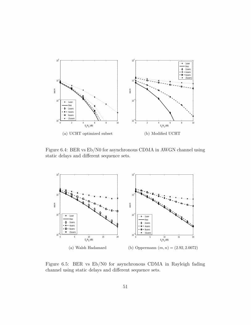
6.4 BER vs Eb/N0 for asynchronous CDMA in AWGN channelusing static delays and different sequence sets. . . . . . . . . . 51

6.5 BER vs Eb/N0 for asynchronous CDMA in Rayleigh fadingchannel using static delays and different sequence sets. . . . . 51

6.6 BER vs Eb/N0 for asynchronous CDMA in Rayleigh fadingchannel using static delays and different sequence sets. . . . . 52

6.7 BER vs Eb/N0 for asynchronous CDMA in AWGN channelusing dynamic delays and different sequence sets. . . . . . . . 54

6.8 BER vs Eb/N0 for asynchronous CDMA in AWGN channelusing dynamic delays and different sequence sets. . . . . . . . 55

6.9 BER vs Eb/N0 for asynchronous CDMA in Rayleigh fadingchannel using dynamic delays and different sequence sets. . . . 56

6.10 BER vs Eb/N0 for asynchronous CDMA in Rayleigh fadingchannel using dynamic delays and different sequence sets. . . . 57

7

List of Tables

1.1 GSM and WCDMA comparison . . . . . . . . . . . . . . . . . 91.2 Sequence applications in modern spread spectrum communi-

cations . . . . . . . . . . . . . . . . . . . . . . . . . . . . . . . 11

2.1 QPSK symbol to bit mapping. . . . . . . . . . . . . . . . . . . 13

4.1 Oppermann sequences showing wide range of correlation prop-erties [15]. . . . . . . . . . . . . . . . . . . . . . . . . . . . . . 37

8

Chapter 1

Introduction

1.1 Multiple Access Technologies

Code Division Multiple Access (CDMA) has gathered widespread recognitionas a standard for multiple access technology. The advance from Global Sys-tem for Mobile (GSM) to Wideband CDMA (WCDMA) is a sort of techno-logical revolution. The tremendous growth in traffic volume and data serviceslead to various modifications in traditional GSM networks. Even addition ofEDGE technology to GSM along with GPRS supports single user data ratesup to 300 kbps whereas WCDMA based 3G network with channel bandwidthof 5 MHz can support data rates up to 2 Mbps [1]. A brief comparison of twotechnologies is presented in Table 1.1. This table clearly reflects the powerand potential of WCDMA in the present and future networks.

Table 1.1: GSM and WCDMA comparisonTechnology Rates

Traditional GSM 14.4kbpsHSCSD (GSM) 28.8kbpsGPRS (GSM) 100kbpsEDGE (GSM) 300kbps

WCDMA 2Mbps

9

1.2 Spreading Sequences

One of the main features of any spread spectrum network is the correlationproperties of spreading sequences employed. Performance of CDMA systemsis strongly dependant on the type of spreading sequences employed, we willshow this in detail in later chapters. To achieve multiple access in CDMAsystems a unique spreading sequence is assigned to each user with optimumcross-correlation properties for a given auto-correlation constraint. When theinformation message is multiplied by the spreading sequence, it transformsit into a wideband spread spectrum signal. This is a very common directsequence spread spectrum technique.

1.3 Challenges and Usage of Sequences

Like any other communication technology CDMA systems also suffer frommany problems. Transmitted radio waves suffer from variations in phase,amplitude and frequency due to various fading conditions of the channel.Channel impact can be mitigated by effective channel estimation techniques.One most common technique is the usage of training sequences or pilot signalwhich also employ sequences. Since transmitted WCDMA signal is superposi-tion of many component signals, for example, pilot channel, common controlchannels and dedicated channels, these signals are added up and if care is nottaken they can give rise to high Peak-to-Average Power Ratio (PAPR) whichwill cause severe problems in the power amplifier. One way to reduce thisPAPR is to select sequences with low PAPR [2]. In asynchronous CDMA,multi users transmitting simultaneously can give rise to interference and canreduce Signal-to-Noise Ratio (SNR) plus interference considerably. One ef-fective way to mitigate this interference is to select sequences with goodaperiodic properties. In Table 1.2, a brief summary of common problemsand sequences employed for their solution in CDMA based communicationsystems is given.

Already different spreading sequences are in use in moder Universal Mo-bile Telecommunications System (UMTS) and we have analyzed some tra-ditional sequences along with new the polyphase sequences as they possessbetter correlation properties as compared to their former counterpart.

10

Table 1.2: Sequence applications in modern spread spectrum communicationsChallenges Solutions

Effect of fading channel Channel estimation using spreading sequencesMulti user interference Mitigate by using sequences with good correlation

Increased PAPR problem Select spreading sequences with better PAPR

1.4 Overview

This thesis is comprised of two main parts. The first part is organized intoChapter 2, 3, and 4, explaining theoretical background of CDMA transmitter,receiver and channel simulators. Chapter 2 presents transmitter and receiverstructures, explaining CDMA signal characteristics, encoding, modulation,demodulation and detection techniques employed. Chapter 3 explains fad-ing radio channel conditions and explains their impact on the system andsome examples of fading in real communication systems. Chapter 4 explainsspreading sequences and their good and optimal criterions along with meritfactors. It also elucidates about better correlation properties of polyphasesequences like Oppermann, UCHT and modified UCHT sequences.

The second part is comprised of Chapters 5, 6 and 7 . It covers simulationmodeling of the system described in previous Chapters. Chapter 5 introducesthe simulation model and simulation environment used in this thesis, whileChapter 6 presents and discusses the results obtained from these simulations.In the last Chapter 7, we conclude our thesis.

11

Chapter 2

Fundamentals of Code DivisionMultiple Access

2.1 Introduction

The transformation of spread spectrum from military to commercial networksresulted in the development of the IS-95 system, which is a Code DivisionMultiple Access (CDMA) based technology. This development led to fur-ther modification in CDMA based systems, culminating in CDMA2000 andWCDMA technology. However, fundamental features of such system remainsthe same. CDMA is a multiple access technology in which different users oc-cupy the same bandwidth at the same time. This shared resource provideschannels on demand to the users. This is the fundamental distinctive featureof CDMA systems as compared to traditional Frequency Division MultipleAccess (FDMA) technologies. CDMA is a spread spectrum based technologyso it is important to define first spread spectrum systems [3]:

“Spread spectrum systems employ excessive signal bandwidth as com-pared to the bandwidth required to send information. This excessive band-width is the spread bandwidth and this spreading is achieved by means of acode. At the receiver the signal is de-spread using synchronized reception ofthe signal with the copy of spreading code.”

We will focus on the main components of simple direct sequence spreadspectrum based CDMA systems in the following sections.

12

2.2 Modulation Scheme

The most common modulation scheme employed in DS-CDMA is quadraturephase shift keying (QPSK). QPSK makes use of both quadrature and inphase components and two components can be included without causinginterference as they are orthogonal to each other. As an example, we have:

∫ nω

0

cos(ωt)sin(ωt)dt = 0, n = 0, 1, 2, 3, .... (2.1)

Higher order modulation schemes are more efficient as in case of QPSK itdoubles the bandwidth efficiency by transmitting two bits in one symbol. TheQPSK system employ numerical symbols to transmit two bits per symbol.In Table 2.1, QPSK symbol to bit mapping is presented [3].

Table 2.1: QPSK symbol to bit mapping.Symbol mapped bits

0 +1, +11 −1, +12 −1,−13 +1,−1

To transmit four different symbols, QPSK needs to send four differentwaveforms. We can call these waveforms as s0, s1, s2 and s3, respectively,and represent them in the form of following the equation:

sn(t) =√

(2E/T )cos(ωt + φ) (2.2)

where n = 0, 1, 2, 3 and φ = π/4, 3π/4, 5π/4, 7π/4 and 0 < t < T . E is thesymbol energy.

QPSK transmits different symbols by simple phase changes. Modulatorinput are data bits and these bits are fed into demultiplexer, here bits areseparated into odd and even bit streams. The in-phase component is multi-plied by even bits and quadrature component multiplies with odd bits andfinally they are combined to have QPSK signal.

At the receiver demodulator separates the input signal into in-phase andquadrature paths and multiplies these components with the reference signals,then the signal is fed into other components of the receiver. QPSK modulatorand de-modulator are shown in Fig. 2.1 and Fig. 2.2.

13

Figure 2.1: QPSK modulator.

Figure 2.2: QPSK demodulator.

14

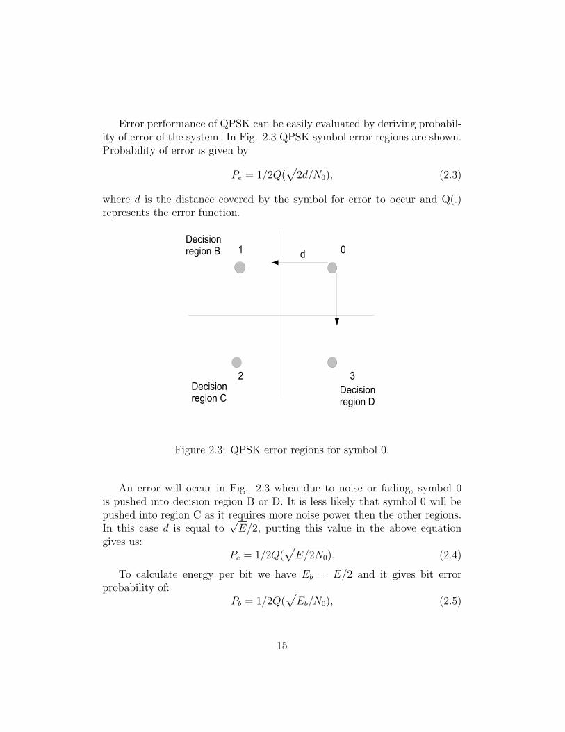
Error performance of QPSK can be easily evaluated by deriving probabil-ity of error of the system. In Fig. 2.3 QPSK symbol error regions are shown.Probability of error is given by

Pe = 1/2Q(√

2d/N0), (2.3)

where d is the distance covered by the symbol for error to occur and Q(.)represents the error function.

Figure 2.3: QPSK error regions for symbol 0.

An error will occur in Fig. 2.3 when due to noise or fading, symbol 0is pushed into decision region B or D. It is less likely that symbol 0 will bepushed into region C as it requires more noise power then the other regions.In this case d is equal to

√E/2, putting this value in the above equation

gives us:Pe = 1/2Q(

√E/2N0). (2.4)

To calculate energy per bit we have Eb = E/2 and it gives bit errorprobability of:

Pb = 1/2Q(√

Eb/N0), (2.5)

15

where Pb is probability of bit error. The probability of symbol error due toshift of symbol 0 to region B and D is therefore twice of probability of biterror.

Ps = Q(√

Eb/N0), (2.6)

where Ps is probability of symbol error.

2.3 Power Control in CDMA

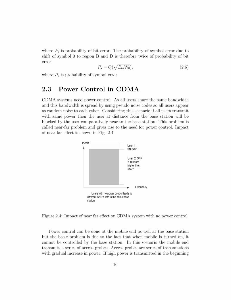
CDMA systems need power control. As all users share the same bandwidthand this bandwidth is spread by using pseudo noise codes so all users appearas random noise to each other. Considering this scenario if all users transmitwith same power then the user at distance from the base station will beblocked by the user comparatively near to the base station. This problem iscalled near-far problem and gives rise to the need for power control. Impactof near far effect is shown in Fig. 2.4

Figure 2.4: Impact of near far effect on CDMA system with no power control.

Power control can be done at the mobile end as well at the base stationbut the basic problem is due to the fact that when mobile is turned on, itcannot be controlled by the base station. In this scenario the mobile endtransmits a series of access probes. Access probes are series of transmissionswith gradual increase in power. If high power is transmitted in the beginning

16

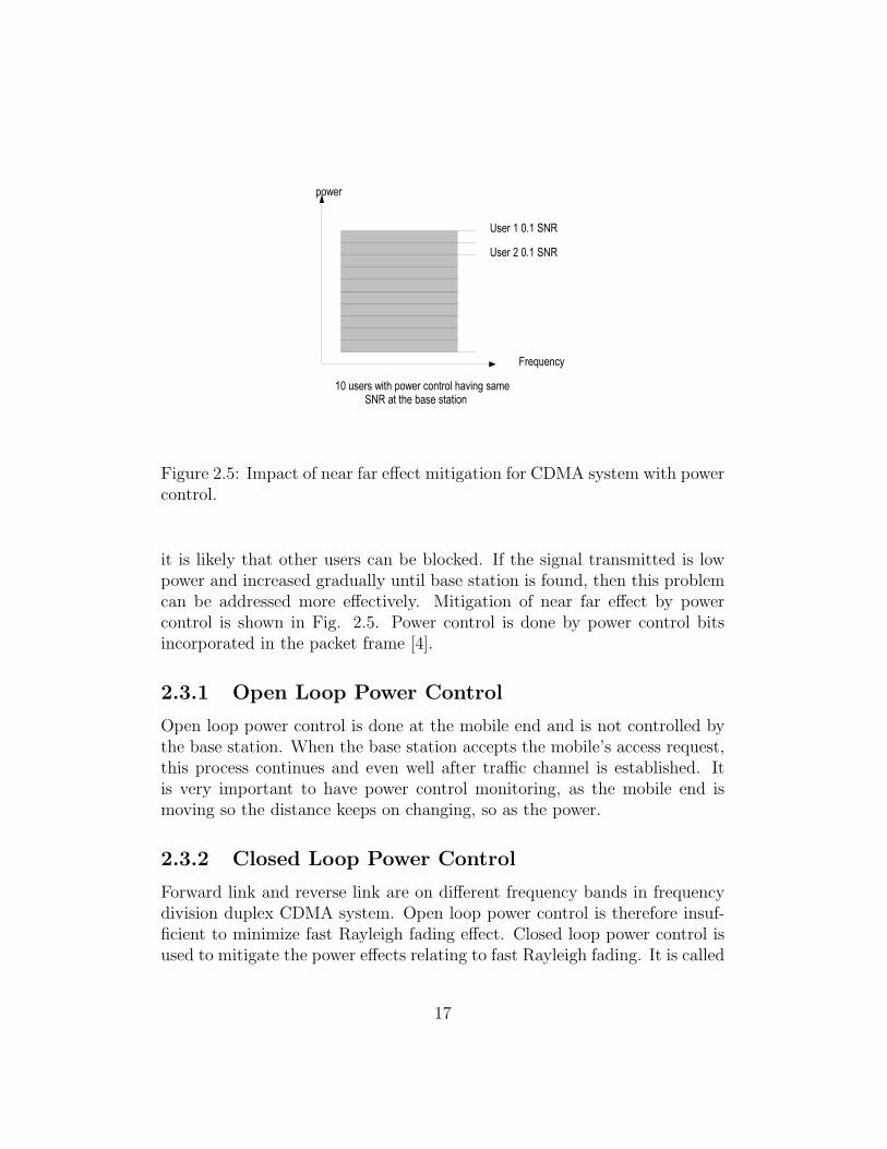
Figure 2.5: Impact of near far effect mitigation for CDMA system with powercontrol.

it is likely that other users can be blocked. If the signal transmitted is lowpower and increased gradually until base station is found, then this problemcan be addressed more effectively. Mitigation of near far effect by powercontrol is shown in Fig. 2.5. Power control is done by power control bitsincorporated in the packet frame [4].

2.3.1 Open Loop Power Control

Open loop power control is done at the mobile end and is not controlled bythe base station. When the base station accepts the mobile’s access request,this process continues and even well after traffic channel is established. Itis very important to have power control monitoring, as the mobile end ismoving so the distance keeps on changing, so as the power.

2.3.2 Closed Loop Power Control

Forward link and reverse link are on different frequency bands in frequencydivision duplex CDMA system. Open loop power control is therefore insuf-ficient to minimize fast Rayleigh fading effect. Closed loop power control isused to mitigate the power effects relating to fast Rayleigh fading. It is called

17

closed loop because both the base station and the mobile end are involved.It takes into effect when once mobile end is on a traffic channel and thenboth base station and mobile end are involved in closed loop power control.Its functioning is very simple to understand. Link quality is monitored con-tinuously, if the link quality is good, base station commands mobile to lowerits power level, and if it is bad then it commands to increase its power level.

2.4 Spreading in CDMA

As mentioned earlier, in CDMA, the transmission bandwidth is much widerthen the minimum user information bandwidth. Individual user bandwidthis spread by a unique wide band code. Generally these spreading codes areorthogonal to each other to avoid multiple user interference at the receiver[5]. Different user wide band signals are added to share the same frequencyspectrum. At the receiver the received signal is despread with the originalcode of the user. The original signal can be spread with variable spreadingfactors. The spreading factor is the ratio of the chip rate to the basebandinformation rate.

Spreading factor =Chip rate

Data rate(2.7)

In case of WCDMA we have 3.84 Mc/s and spreading factor for 15 ksym/sis given by:

3.84

15Mchips/ksymbols = 256 spreading factor (SF) (2.8)

2.5 CDMA Signal Model

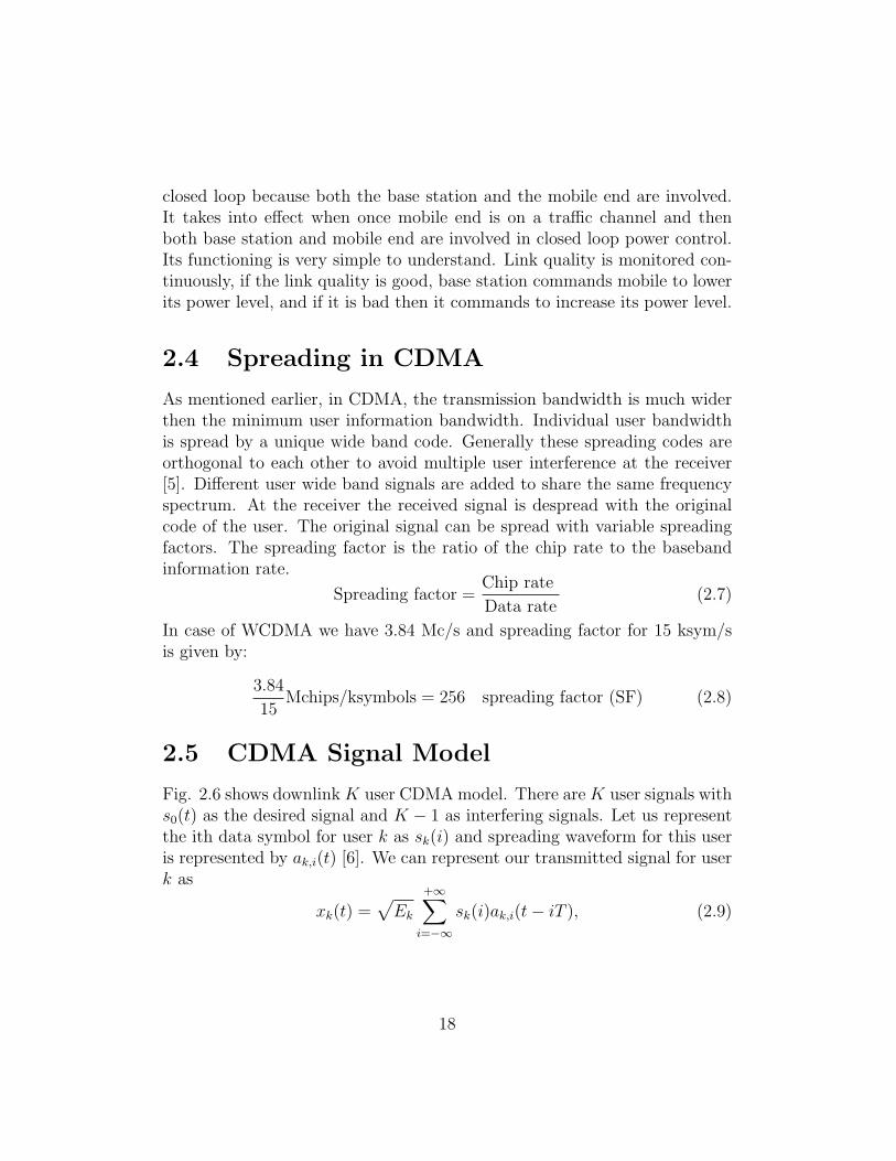
Fig. 2.6 shows downlink K user CDMA model. There are K user signals withs0(t) as the desired signal and K − 1 as interfering signals. Let us representthe ith data symbol for user k as sk(i) and spreading waveform for this useris represented by ak,i(t) [6]. We can represent our transmitted signal for userk as

xk(t) =√

Ek

+∞∑i=−∞

sk(i)ak,i(t− iT ), (2.9)

18

Figure 2.6: Downlink K user CDMA model

where Ek is symbol energy and T is the symbol duration. The spreadingwaveform is represented by:

ak,i(t) = 1/√

N

N−1∑j=0

ck,i(j)p(t− jTc) (2.10)

here Tc is the chip duration and chip pulse is convolved with the chip shapepulse. We are considering orthogonal codes for downlink so:

cHk,icj,i = 0, (2.11)

where k 6= j and H is Hermitian transpose.The K users will contribute similar signal sets as shown in above equa-

tions. At the receiver for s0(t) as the desired signal, there will be desiredsignal plus multi user interference and noise. It can be easily represented by:

r(t) =K−1∑

k=1

L−1∑

l=0

glxk(t− τ) + n(t), (2.12)

where gl is the channel response and n(t) is the additive noise. By de-spreading the s0(t) desired signal with the users known spreading code, onecan get rid of multiple access interference. The effective choice of sequenceswill impact the performance of the system.

19

Chapter 3

Radio Channels

3.1 Introduction

Radio channels place basic limits on the performance of wireless systems. Aradio channel can be of variety of types and it can change with time. Thisrandom nature of radio channels make them very important in the wirelesstransmission systems. In traditional systems we experience additive whiteGaussian noise (AWGN) channel model with thermal noise in the receivercomponents along with antenna temperature as the main source of signaldegradation [7]. In radio channels, this model fails due to the random natureof propagation channel.

This random nature causes rapid changes in signals amplitude, phaseand frequency and is generally called fading. More importantly in a wirelesschannel, a signal can travel over multiple paths between transmitter andreceiver and can contribute to multi path fading.

3.2 Fading Models

Channel modeling is generally based on large and short area distances. Mod-els based on large area distances cover mean signal strength of the signal andare efficient in measuring radio coverage area in broader aspects. Such prop-agation models are termed as large scale propagation models. On the otherhand, models based on rapid changes of signal strength over short areas andtime are termed as small scale fading [8]. Main types of radio channel fadingare classified in Fig. 3.1.

20

Figure 3.1: Types of fading in radio channels.

21

3.2.1 Large Scale Fading

Impact of surrounding terrain, infrastructure and landscape on received sig-nal strength are described in large scale fading model. This is described interms of mean path loss nth-power law and a log normally-distributed varia-tion about the mean [7]. Mean path loss as a function of distance ‘d’ betweenmobile end and base station can be expressed as:

Lp(d) ∝ (d/dr)n, (3.1)

where Lp is the path loss, dr is reference distance generally in the range of100 m to 1 km depending on the size of cell and value of path loss exponentn depends on propagation environment and generally lies between 2 and 4.

Measured values have shown that path loss is a random variable witha log-normal distribution. So, in more appropriate terms we can generalizelarge scale fading model as:

Lls = Lp(d) + Yσ, (3.2)

where Yσ is deviation about the mean.

3.2.2 Small Scale Fading

Small scale fading is caused by multi path in the radio channel. It can causefading in received signal in three main ways [8]:

1. Fast changes in received signal over a short period of time or distance.

2. Due to time varying channel various Doppler shifts can cause frequencymodulation of the signal.

3. Multi path delays can generate echoes of the signal.

If the received signal is composed of line of sight and non line of sight (scat-tered) components then this small scale fading is called Ricean fading. If theline of sight component in the received signal is zero then it is called Rayleighfading. An example of a Rayleigh fading envelope is shown in Fig. 3.2.

Rayleigh fading follow Rayleigh probability density function given as:

p(r) =

{rσ2 e

[−r2/2σ2] for r ≥ 0,

0 otherwise.(3.3)

In our study for this thesis we have assumed that fading channel is fol-lowing flat Rayleigh fading and we have considered baseband model.

22

0 2 4 6 8 1010

−3

10−2

10−1

100

Rece

ived

field

inten

sity (

dB)

time

Figure 3.2: A typical Rayleigh fading envelope.

3.3 Small Scale Fading: Mechanisms, Degra-

dation Categories and Effects

Variations of signal arriving with different delays can be considered uncor-related. A signal model based on such assumptions can be effectively widesense stationary. In case of radio channels such a model can be explainedwith the help of four functions. We are going to consider these four functionsand their impact on the radio channels in the next sections.

3.3.1 Time Dispersion in Time Delay Domain

Time dispersion can be observed by plotting received power of the transmit-ted signal varying with time delay τ . We can define τ as the copy of signalcomponent received after the first signal arrival. For some channels thesemulti path components can be continuous. We can define maximum excessdelay Tm as the time during which first and last multipath component ofthe transmitted signal is received. If we compare Tm with symbol time Ts,we can observe that our signal is distorted in two main ways and they areexplained in the subsequent sections.

23

3.3.2 Frequency Selective Fading

If Tm > Ts, then it means that received multi path is extending beyond thesymbol time duration so it will cause channel related inter symbol interfer-ence (ISI). This kind of fading is termed as frequency selective fading. InCDMA systems, RAKE receiver fingers are used to resolve these multi pathcomponents.

3.3.3 Flat Fading

If Tm < Ts, then it means that all the received multipath components arearriving within the symbol time period. So, there is no inter symbol interfer-ence (ISI) but still the received components can add destructively and causevariations in received signal. This type of fading is termed as flat fading andit results in the loss of SNR.

3.3.4 Time Dispersion in Frequency Domain

Fourier transform of received power intensity versus time delay τ gives usfrequency representation of time dispersion. It can be defined as the correla-tion measure of channels response to two signals as a function of frequencydifference. The coherence bandwidth f0 is the measure of such function. Itis define as the bandwidth over which the channel passes transmitted signalswith approximately equal gains.

f0 ≈ 1/Tm (3.4)

It is reciprocal of maximum excess delay Tm. An absolute relationship amongf0 and delay spread does not exist. But we can approximate the relationshipby the following expression:

f0 ≈ 1/50στ (3.5)

where στ is the delay spread given by:

στ =√

τ 2 − (τ)2 (3.6)

where τ is mean excess delay and (τ)2 is mean squared delay.

24

3.3.5 Frequency Selective Fading in Frequency Domain

If f0 < W , where W is the bandwidth and 1Ts≈ W , then some of the signal

spectral components will fall outside the coherence bandwidth giving rise tofrequency selective channel.

3.3.6 Flat Fading in Frequency Domain

If f0 > W then all spectral components of the transmitted signal will fallinside the coherence bandwidth and it will give rise to flat fading.

3.3.7 Time Variance of the Channel in Time Domain

Time variation of the channel can be defined as either relative motion oftransmitter and receiver with respect to each other or the motion of objectsin the channel. Due to variations in channel signal amplitude and phase arevaried as channel propagation paths are constantly changing. The coherencetime T0 is the measure of time variation. It is define as the time over whichthe channel remains constant.

3.3.8 Fast Fading

If Ts > T0, then channel is said to be fast fading. It means that symbol timeperiod is greater than coherence time T0.

3.3.9 Slow Fading

If Ts < T0, then channel is said to be slow fading and it means that channelis staying constant over the symbol time period.

3.3.10 Time Variance of the Channel in Frequency(Doppler) Domain

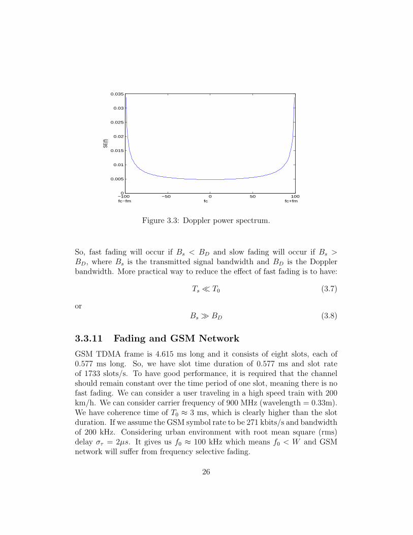
When coherence time period is shorter than symbol time period, then itgives rise to Doppler spreading in frequency domain also called time selectivefading. A Doppler power spectrum is shown in Fig. 3.3. When viewedin the frequency domain, signal distortion due to fast fading increases withincreasing Doppler spread relative to the bandwidth of the transmitted signal.

25

−100 −50 0 50 1000

0.005

0.01

0.015

0.02

0.025

0.03

0.035

fc−fm fc fc+fm

SE(f)

Figure 3.3: Doppler power spectrum.

So, fast fading will occur if Bs < BD and slow fading will occur if Bs >BD, where Bs is the transmitted signal bandwidth and BD is the Dopplerbandwidth. More practical way to reduce the effect of fast fading is to have:

Ts ¿ T0 (3.7)

orBs À BD (3.8)

3.3.11 Fading and GSM Network

GSM TDMA frame is 4.615 ms long and it consists of eight slots, each of0.577 ms long. So, we have slot time duration of 0.577 ms and slot rateof 1733 slots/s. To have good performance, it is required that the channelshould remain constant over the time period of one slot, meaning there is nofast fading. We can consider a user traveling in a high speed train with 200km/h. We can consider carrier frequency of 900 MHz (wavelength = 0.33m).We have coherence time of T0 ≈ 3 ms, which is clearly higher than the slotduration. If we assume the GSM symbol rate to be 271 kbits/s and bandwidthof 200 kHz. Considering urban environment with root mean square (rms)delay στ = 2µs. It gives us f0 ≈ 100 kHz which means f0 < W and GSMnetwork will suffer from frequency selective fading.

26

3.3.12 Fading and WCDMA Network

WCDMA frame typically is 10 ms long and it consists of 15 slots, each of0.667 ms long. So, we have slot time duration of 0.667 ms and slot rateof 1499 slots/s. Considering again a user in a fast moving train with speedapproaching 200 km/h. Assuming a down link carrier frequency of 2110 MHz(wavelength= 0.142 m). We have coherence time of T0 ≈ 1.28 ms, which isclearly higher than the slot duration. It means channel remains constantover slot interval. If we assume WCDMA chip rate to be 3.84 chips/s andbandwidth of 5 MHz channels. Again considering urban environment withrms delay στ = 2µs. It gives us f0 ≈ 100 kHz which means f0 ¿ W andCDMA network will suffer from multi path fading. In fact these multi pathsare used as diversity components in RAKE receivers of CDMA networks.

27

Chapter 4

Spread Spectrum SpreadingSequences

4.1 Introduction

A signal can be considered as the change of any measurable quantity thatdelivers information regarding the behavior of the related source or process.The sequence is described as a signal with continuous or discrete parameterchanges and discrete time variability [10].

One simple way to classify sequences is related to their member elements.A discrete time continuous valued sequence b = [bn] is called a real sequenceif the members of elements are real numbers and a complex sequence if themembers of elements are complex. If all members are complex root of unity

i.e. bn = ei2πxn

q then its called polyphase sequence. Similarly, a discrete timesignal is called a multilevel sequence if it has p possible discrete values, if ithas only two values then it is called a binary sequence. The two values canbe either 0 and 1 or +1 and -1.

4.2 Correlation Functions and Related

Sequences

Correlation functions are the fundamental properties which are used to char-acterize different sequences or different sets of sequences. Correlation ofsignals or sequences is a measurement of degree of similarity of one signal or

28

sequence to the other or to itself.We will divide our correlation functions into two major groups i.e. peri-

odic correlation functions and aperiodic correlation functions [11].

4.2.1 Periodic Correlation Functions

Discrete periodic correlations have the following characteristics [10]:

1. The Rac i.e. auto-correlation is the degree of measurement of dependenceof one sequence on itself, its value at zero delay is the sum of squared valuesof its elements:

Rk(0) =N−1∑n=0

bn2 (4.1)

2. The Rac is an even function of the delay τ :

Rk(−τ) = Rk(τ) (4.2)

3. The maximum autocorrelation occurs at τ = 0:

Rk(0) ≥ Rk(τ), τ 6= 0 (4.3)

4. The Rcc i.e. cross-correlation is the degree of measurement of similarityof one sequence on other, its value is not necessarily maximum at τ = 0 andis not necessarily an even function.

5. The symmetrical property of Rcc is:

Rk,j(τ) = Rj,k(−τ) (4.4)

29

4.2.2 Aperiodic Correlation Functions

Aperiodic correlation functions are important when systems are operatingin asynchronous mode. For sequences b = [bn] and c = [cn] of length N,where N are not always single period of periodic sequences, we can defineour aperiodic correlation function as

Ck,j(τ) =

∑N−1−τn=0 bncn+τ , 0 ≤ τ ≤ N − 1,∑N−1+τn=0 bn−τcn, 1−N ≤ τ ≤ 0,

0, τ > N.

(4.5)

1. Aperiodic Cac and Ccc have in-phase values equal to corresponding periodicauto-correlation and cross-correlation values:

Ck,j(0) = Rk,j(0), Ck(0) = Rk(0) (4.6)

2. It also follows the symmetrical properties, that is

Ck,j(−τ) = Ck,j(τ)∗, Ck(−τ) = Ck(τ)∗ (4.7)

where * represents complex conjugate.

4.3 Fundamental Requirements of Sequences

Many requirements of sequences are dependent on the type of applications inwhich they are employed. But there are some basic characteristics importantfor a sequence or a sequence set to have good properties.

1. The number of elements in a period of length N.

2. Sequence sets, i.e. number of sequences in a set M.

3. For periodic sequences it is important to have minimum imbalancebetween number of symbols.

4. If Ram is the maximum out-of-phase auto-correlation and Rcm is themaximum cross-correlation, then Rmax is called the maximum nontrivialcorrelation value.

30

Rmax = max(Ram, Rcm) (4.8)

5. Linear span is the measure of predictability of the sequence. It isrequired that generally any pseudo random sequence should have largelinear span compared with its period.

6. For minimum interference in spread spectrum based systems and forefficient synchronization it is necessary to have lower value of Rmax.

4.3.1 Bounds on Sequences

To have lower bound on the minimum value of Rmax, we have [10]

1. Sarwate bound is given by:

R2cm

N+

(N − 1)R2am

(M − 1)N2≥ 1 (4.9)

2. Welch calculated the following bound:

Rmax ≥ N

√(M − 1)

(NM − 1)(4.10)

4.3.2 Merit Factor and Energy Efficiency

An important feature of aperiodic autocorrelation is the ratio of energy ofautocorrelation function (ACF) main lobes to the energy of ACF side lobes[10]. It is beneficial to have large merit factor. The merit factor is definedas:

Merit factor =C2

k(0)

2∑N−1

τ=1 C2k(τ)

(4.11)

Another important property for sequence design is the energy efficiency ofsequences. If a sequence has constant amplitude, then it has highest possibleenergy efficiency of 1. The energy efficiency is defined as

Energy efficiency =

∑N−1n=0 b2

n

Nmax(b2n)

(4.12)

31

4.3.3 Advantage of Polyphase Sequences

Sidelnikov bound explains us that on approximation we can have 3dB ad-vantage depending upon sequence set, if we use non-binary sequences. Whensize of sequence set is M = Nu , N À u and u ≥ 1 is an integer, thenfor sequence sets having M ≈ N and u ≈ 1, we have maximum non trivialcorrelation value:

Rmax ≥√

2N, for binary sequences (4.13)

Rmax ≥√

N, for non-binary sequences (4.14)

4.4 Orthogonal Spreading Sequences

Orthogonal sets of sequences provide great advantage in systems where syn-chronization can be achieved. As orthogonal sets of sequences have cross-correlation Rcc = 0 at τ = 0. So, in synchronized systems they can reducemultiple access interference (MAI) significantly. In present CDMA based 3Gsystems, Walsh Hadamard orthogonal sets of sequences are applied in thesynchronous down link of CDMA. These sets of sequences are easy to gen-erate and can be easily extended to larger sets of sequences. So, these setsof sequences do fulfill many properties mentioned above as requirements forgood sequence sets. But unfortunately Walsh Hadamard sequences have badautocorrelation properties, so their use can lead to synchronization and codetracking errors. Typical correlation functions of Walsh Hadamard sequencesare shown in Fig. 4.1. In real scenarios different techniques are employed tomitigate this bad ACF. One such technique can be the use of sequence setswith better auto-correlation properties.

Moreover, in asynchronous scenarios which are more often encounteredin real systems the property of orthogonality is lost. In such cases it is moreuseful to have lower cross-correlation side lobes, i.e out-of-phase correlationfunctions gain significant importance. Therefore, it is generally desired tohave sequences with better ACF and CCF properties .

32

−40 −30 −20 −10 0 10 20 30 400

0.5

1

Ra

c

Auto−correlation of sequence 1

−40 −30 −20 −10 0 10 20 30 400

0.5

1

Ra

c


−40 −30 −20 −10 0 10 20 30 400

0.5

1

Rcc

Cross−correlation between sequence 1 and 12

−40 −30 −20 −10 0 10 20 30 400

0.5

1

Chip delays

Rcc

Cross−correlation between 3 and 12

Figure 4.1: Typical correlations of Walsh Hadamard sequences of length 32.

33

4.5 Unified Complex Hadamard Transform

Sequences

As stated previously, non-binary sequences can give 3dB advantage over bi-nary sequences. Unified Complex Hadamard Transform (UCHT) sequencesare polyphase sequences and like Walsh Hadamard sequences, UCHT se-quences are based on Hadamard transform. As a result they are very easy togenerate and can be manipulated very easily with the current Digital SignalProcessors (DSP) [12]and [13]. A UCHT matrix U of order is a square matrixwith elements ±1 and ±i and is constructed by:

Un = U1

⊗, . . . ,

⊗︸︷︷︸

n times

U1, (4.15)

where U1 is defined as:

U1 =

[µ1 µ1µ3

µ2 −µ2µ3

], (4.16)

where µ1, µ2, µ3 ∈ {1,−1, i,−i}, and i =√−1.

There are 64 different U1 matrices [12]. Based on whether µ3 is imaginaryor not, 32 matrices are called half symmetry property matrices (HSP) andthe rest 32 are called non half symmetry property matrices (N-HSP). Forexample, if n = 1 and µ1 = 1, µ2 = −i and µ3 = i, we have:

U1 =

[1 i−i −1

](4.17)

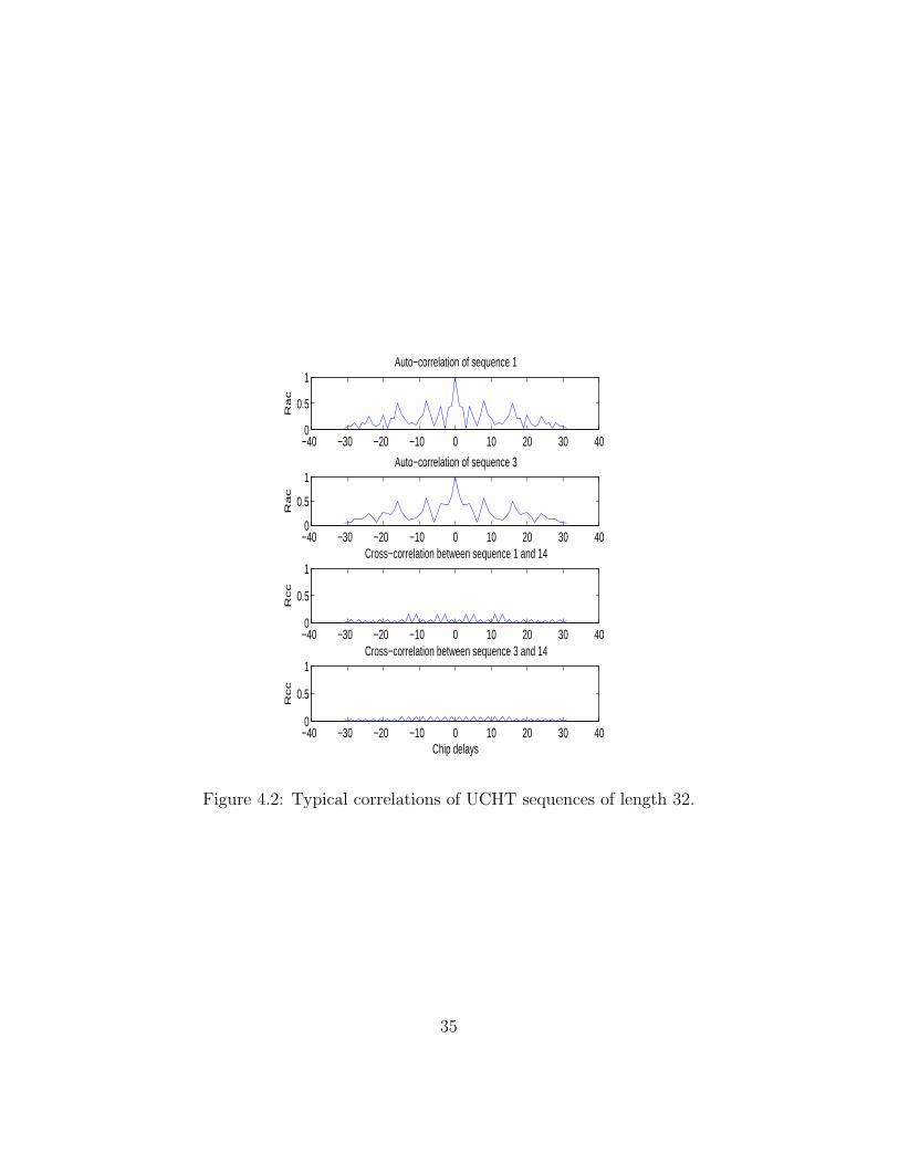
The rows of the UCHT matrix represent the UCHT sequences. UCHTsequences are orthogonal, so in synchronous down link they can reduce MAIand also their auto-correlation is better than Walsh Hadamard sequences.Typical correlation functions of UCHT sequences are shown in Fig. 4.2.

4.6 Modified UCHT Sequences

Cross-correlation function of UCHT sequences varies within a set as it can beseen from Fig. 4.2. It can reach an upper bound of 0.7 which is highly unde-sirable in case of asynchronous CDMA system. To further extend the design

34

−40 −30 −20 −10 0 10 20 30 400

0.5

1

Ra

c


−40 −30 −20 −10 0 10 20 30 400

0.5

1

Ra

c


−40 −30 −20 −10 0 10 20 30 400

0.5

1

Rcc


−40 −30 −20 −10 0 10 20 30 400

0.5

1

Chip delays

Rcc


Figure 4.2: Typical correlations of UCHT sequences of length 32.

35

set of UCHT,[14] presents a method to extend the construction of UCHTsequences and such sequence sets are called modified UCHT sequence sets.Modified UCHT sequences have already been shown to be good candidate formulti carrier CDMA [2]. These sequences are also orthogonal and decreasethe upper bound on cross-correlation of UCHT sequences and also providebetter auto-correlation properties. Typical correlation functions of modifiedUCHT sequences are shown in Fig. 4.3.

−40 −30 −20 −10 0 10 20 30 400

0.5

1

Ra

c


−40 −30 −20 −10 0 10 20 30 400

0.5

1

Ra

c


−40 −30 −20 −10 0 10 20 30 400

0.5

1

Rcc


−40 −30 −20 −10 0 10 20 30 400

0.5

1

Chip delays

Rcc


Figure 4.3: Typical correlations of modified UCHT sequences of length 32.

The transformation core matrix of a modified UCHT matrix shall bedefined as Un = UnDn. Here Un is the original UCHT matrix and Dn is themodifying matrix.

The modifying diagonal matrix is given by

Dn = diag[e2iπd1 , . . . , e2iπdN ]. (4.18)

36

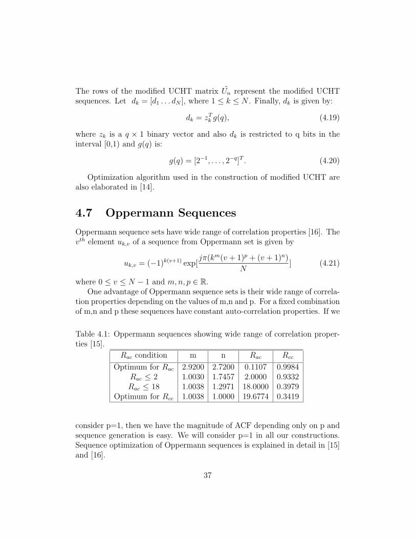
The rows of the modified UCHT matrix Un represent the modified UCHTsequences. Let dk = [d1 . . . dN ], where 1 ≤ k ≤ N . Finally, dk is given by:

dk = zTk g(q), (4.19)

where zk is a q × 1 binary vector and also dk is restricted to q bits in theinterval [0,1) and g(q) is:

g(q) = [2−1, . . . , 2−q]T . (4.20)

Optimization algorithm used in the construction of modified UCHT arealso elaborated in [14].

4.7 Oppermann Sequences

Oppermann sequence sets have wide range of correlation properties [16]. Thevth element uk,v of a sequence from Oppermann set is given by

uk,v = (−1)k(v+1) exp[jπ(km(v + 1)p + (v + 1)n)

N] (4.21)

where 0 ≤ v ≤ N − 1 and m,n, p ∈ R.One advantage of Oppermann sequence sets is their wide range of correla-

tion properties depending on the values of m,n and p. For a fixed combinationof m,n and p these sequences have constant auto-correlation properties. If we

Table 4.1: Oppermann sequences showing wide range of correlation proper-ties [15].

Rac condition m n Rac Rcc

Optimum for Rac 2.9200 2.7200 0.1107 0.9984Rac ≤ 2 1.0030 1.7457 2.0000 0.9332Rac ≤ 18 1.0038 1.2971 18.0000 0.3979

Optimum for Rcc 1.0038 1.0000 19.6774 0.3419

consider p=1, then we have the magnitude of ACF depending only on p andsequence generation is easy. We will consider p=1 in all our constructions.Sequence optimization of Oppermann sequences is explained in detail in [15]and [16].

37

In mainly two schemes we can summarize optimization for Oppermannsequences

1. Optimization for ACF with high CCF values

2. Optimization for CCF with high out of phase ACF values.

−30 −20 −10 0 10 20 300

0.5

1

Ra

c

Auto−correlation of sequence 1 for(m,n)=(2.92,2.0072)

−30 −20 −10 0 10 20 300

0.5

1

Ra

c

Auto−correlation of sequence 2 for (m,n)=(2.92,2.0072)

−30 −20 −10 0 10 20 300

0.5

1

Rcc

Cross−correlation between sequence 3 and 4 for (m,n)=(1.0038,1.2971)

−30 −20 −10 0 10 20 300

0.5

1

Chip delays

Rcc

Cross−correlation between sequence 4 and 5 for (m,n)=(1.0038,1.2971)

Figure 4.4: Typical correlations of Oppermann sequences of length 31 of twodifferent sets.

It is very obvious from Fig. 4.4 that sequences with low mean out-of-phaseACF approximates a delta function, giving a wide and flat frequency spec-trum which is desirable in spread spectrum systems. But this advantage isgained at the expense of large CCF values which are different for differentsequences. However, it is possible to define regions of low mean out of phaseauto-correlation with sufficient cross-correlation. This problem can be solvedby considering two dimensional optimization problem as defined in [15].

38

Chapter 5

Simulation Environment

5.1 Introduction

Performance of spreading sequences in a DS-CDMA system are simulated inadditive white Gaussian channel (AWGN) and fading channel. The preced-ing chapters gave a comprehensive background of CDMA system, complexspreading sequences and fading channels. Using this background it is possi-ble to build a simulation software package to simulate a CDMA based systemover a fading channel using different families of complex spreading sequences.We can evaluate the performance of each family and determine their poten-tial to be used in future spread spectrum based communication standards[19].

In this Chapter, we will present the simulation model used in this thesis.We have used Matlab programming to build this simulation software.

5.2 Synchronous CDMA Downlink System Model

We have divided our model in synchronous down-link and asynchronous up-link CDMA system. As explained in Chapter 4, orthogonal sequences provideexcellent performance for synchronous downlink CDMA system. Our modelcan simulate up to K = 30 users operating simultaneously in the synchronousenvironment [8]. Fig. 5.1(a) and 5.1(b) display synchronous transmitter andreceiver block, respectively. In the transmitter block, user’s information dataare QPSK modulated and spread by its corresponding spreading sequence.The sequences used have length N = 31 or 32 and include:

39

Figure 5.1: (a) Synchronous transmitter and (b) receiver block.

1. Walsh Hadamard sequences

2. Oppermann sequences

3. UCHT sequences

4. Modified UCHT sequences.

The channel is modeled as flat and slow Rayleigh fading with AWGN tomodel thermal noise at the receiver. Signals are transmitted through thechannel with different energy per bit to noise ratio Eb/N0. In our model,Eb/N0 varies between 0 dB to 20 dB. At the receiver, the received signal ismatched to a fading channel filter and de-spread for a particular user, thenintegrated and dumped. Finally hard decision device is used on real andimaginary parts of complex symbols to generate bit error rate (BER).

5.3 Asynchronous CDMA Uplink System

Model Using Static Delays

Uplink of CDMA systems are asynchronous, as it is very difficult to syn-chronize different mobile stations working independent of each other. In our

40

Figure 5.2: (a) Asynchronous transmitter and (b) receiver block.

asynchronous uplink system model the only difference is the introduction ofstatic delays at the transmitter. The rest of the model follows the steps asdescribed in the previous section. Fig. 5.2(a) and 5.2(b) explains completeasynchronous transmitter for K users and K = 1 user receiver.

5.4 Asynchronous CDMA Uplink System

Model Using Random Dynamic Delays

In real scenarios, asynchronous systems generally suffer from dynamic delaysrather than static delays. Our simulations also include random dynamicdelay model [20]. In this model, we have delayed our users randomly andthen within each random delay dynamic delays are given to each user withincertain limit. At the receiver side, first average BER within dynamic delaylimit is calculated within each SNR and then BER is evaluated for differentSNR’s in traditional way. All other steps on the transmitter and receiver sidein the simulation model follow the preceding sections. Fig. 5.3(a) and 5.3(b)displays all the necessary steps involved in the simulations on transmitter andreceiver sides. Dynamic delay models result in slightly more deterioration inperformance for sequences as compared to static delay models.

41

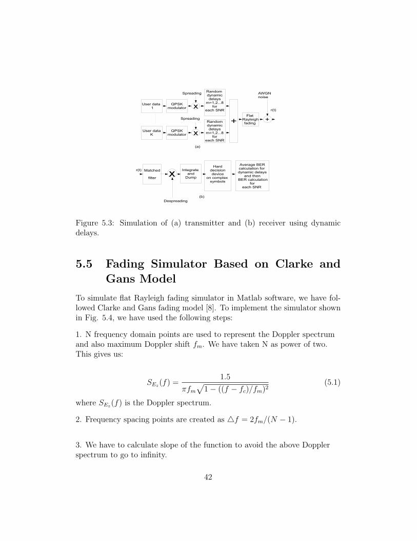
Figure 5.3: Simulation of (a) transmitter and (b) receiver using dynamicdelays.

5.5 Fading Simulator Based on Clarke and

Gans Model

To simulate flat Rayleigh fading simulator in Matlab software, we have fol-lowed Clarke and Gans fading model [8]. To implement the simulator shownin Fig. 5.4, we have used the following steps:

1. N frequency domain points are used to represent the Doppler spectrumand also maximum Doppler shift fm. We have taken N as power of two.This gives us:

SEz(f) =1.5

πfm

√1− ((f − fc)/fm)2

(5.1)

where SEz(f) is the Doppler spectrum.

2. Frequency spacing points are created as 4f = 2fm/(N − 1).

3. We have to calculate slope of the function to avoid the above Dopplerspectrum to go to infinity.

42

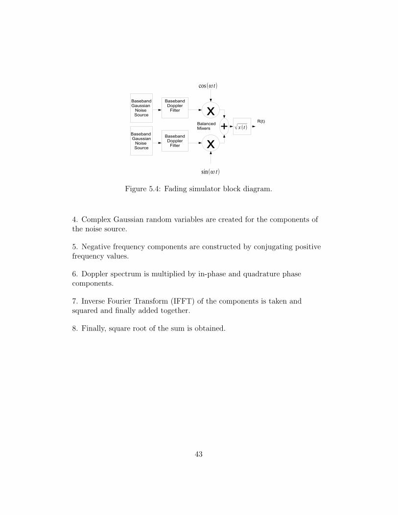
Figure 5.4: Fading simulator block diagram.

4. Complex Gaussian random variables are created for the components ofthe noise source.

5. Negative frequency components are constructed by conjugating positivefrequency values.

6. Doppler spectrum is multiplied by in-phase and quadrature phasecomponents.

7. Inverse Fourier Transform (IFFT) of the components is taken andsquared and finally added together.

8. Finally, square root of the sum is obtained.

43

Chapter 6

Simulation of a DS-CDMASystem

6.1 Simulation Results

In this chapter, we will discuss the simulation results generated with thehelp of Matlab. We will explain our results for AWGN and Rayleigh fadingchannels separately. All necessary plots are shown in Section 6.2.

6.1.1 AWGN Channel

Theoretical BER limit for AWGN channel is discussed in Chapter 2. Our sim-ulation results conclude that sequences optimized for low mean square cross-correlation values give much better performance, when simulated for BERas compared to those optimized for low mean square auto-correlation. Thisresult is consistent for a DS-CDMA based system. This low cross-correlationamong spreading sequences gives rise to less multiple access interference.

6.1.2 Rayleigh Fading Channel

We have extended our model to include Rayleigh fading as well, and oursimulation results indicate that performance of sequences is poor for fadingchannel as compared to AWGN channel. The theoretical probability of error

44

limit for fading channel based on QPSK system is [19]

PeR= 1−

√(Eb/N0)

(1 + Eb/N0)(6.1)

For synchronous downlink our model is using orthogonal and near or-thogonal sequences. This results in sufficient multiple access interference(MAI) reduction and our numerical results follow theoretical limit for allsequence sets. In case of asynchronous up-link, simulation plots clearly indi-cate that Oppermann sequences with (m,n) = (1.0038, 1.2971) outperformother sequences, when simulated for 15 users. Sequences optimized for auto-correlation seem to perform worst. In case of UCHT sequences, we canconclude that some sequences outperform traditional Walsh Hadamard se-quences. Overall, set of modified UCHT sequences give consistent BER per-formance for 15 users but perform poorly as compared to optimized subsetsof other sequences.

For synchronous downlink DS-CDMA system, our model is using orthog-onal and near orthogonal sequences. This results in sufficient MAI reductionand our numerical results follow theoretical limit for all sequence sets. In caseof asynchronous down-link Oppermann sequences with low cross-correlationvalues seem to outperform other sequence sets. Some UCHT sequences out-perform Walsh Hadamard sequences for higher number of users. ModifiedUCHT sequences with better auto-correlation and minimized upper boundcross-correlation function as compare to UCHT sequences, give consistentBER performance for 15 users but give bad perform as compared to opti-mized subsets of all sequence sets used in our simulation model. In dynamicdelay environment modified UCHT sequences slightly outperform UCHT andWalsh Hadamard sequences, in case of random selection of sequences with ina set. But loose this advantage when optimized subsets of the same sequencesets are used.

45

6.2 Results

6.2.1 Synchronous CDMA Simulation Results

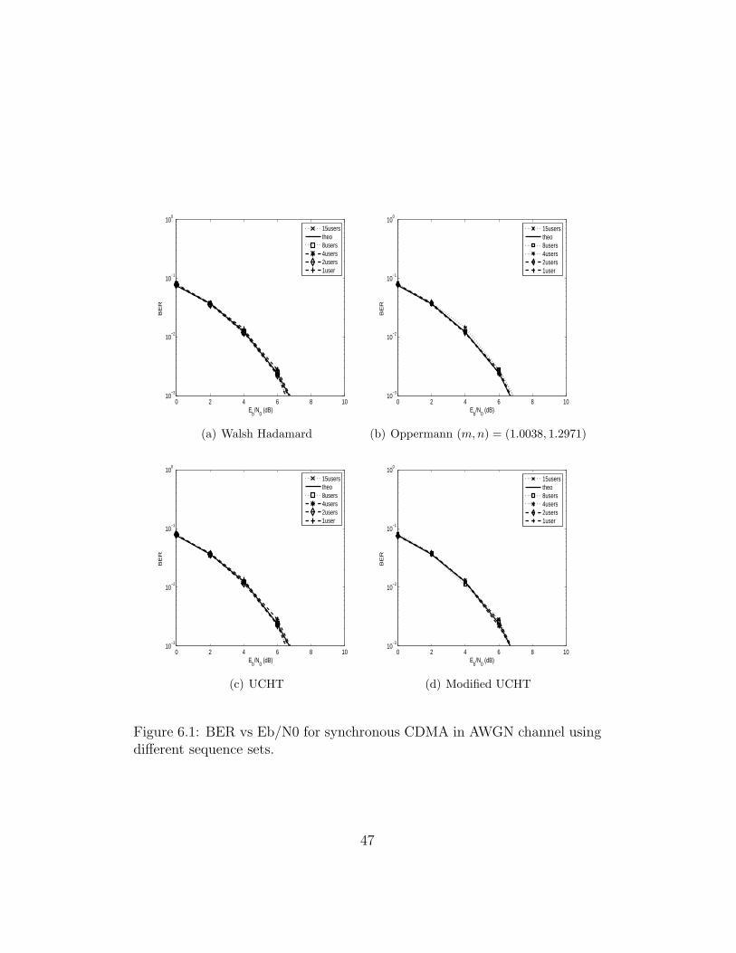
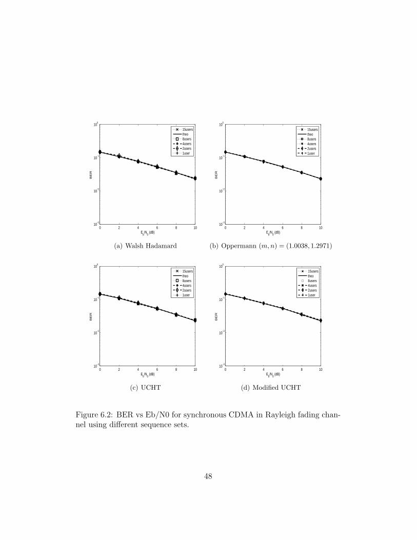
Simulations for synchronous downlink CDMA system clearly reflect the ad-vantage of orthogonal sequences like Walsh Hadamard, UCHT, modifiedUCHT and near orthogonal sequences like Oppermann sequences. All thesesets of sequences achieve theoretical BER limit even in the presence of 15users transmitting at the same time in both AWGN and Rayleigh fadingchannels. In all our simulation figures (theo) represents theoretical BER forrespective AWGN and Rayleigh fading channels for QPSK modulated sys-tems. Fig. 6.1 and Fig. 6.2 clearly shows that in downlink synchronousCDMA, orthogonal and near orthogonal sets of sequences can sufficientlymitigate multiple access interference and provide optimum performance.

46

0 2 4 6 8 1010

−3

10−2

10−1

100

Eb/N

0 (dB)

BE

R

15userstheo8users4users2users1user

(a) Walsh Hadamard

0 2 4 6 8 1010

−3

10−2

10−1

100

Eb/N

0 (dB)

BE

R


(b) Oppermann (m,n) = (1.0038, 1.2971)

0 2 4 6 8 1010

−3

10−2

10−1

100

Eb/N

0 (dB)

BE

R


(c) UCHT

0 2 4 6 8 1010

−3

10−2

10−1

100

Eb/N

0 (dB)

BE

R


(d) Modified UCHT

Figure 6.1: BER vs Eb/N0 for synchronous CDMA in AWGN channel usingdifferent sequence sets.

47

0 2 4 6 8 1010

−3

10−2

10−1

100

Eb/N

0 (dB)

BE

R


(a) Walsh Hadamard

0 2 4 6 8 1010

−3

10−2

10−1

100

Eb/N

0 (dB)

BE

R


(b) Oppermann (m,n) = (1.0038, 1.2971)

0 2 4 6 8 1010

−3

10−2

10−1

100

Eb/N

0 (dB)

BE

R


(c) UCHT

0 2 4 6 8 1010

−3

10−2

10−1

100

Eb/N

0 (dB)

BE

R


(d) Modified UCHT

Figure 6.2: BER vs Eb/N0 for synchronous CDMA in Rayleigh fading chan-nel using different sequence sets.

48

6.2.2 Asynchronous CDMA Simulation Results

In asynchronous scenarios our simulation results show deterioration for largenumber of users. As all sequence sets loose orthogonality when subjected tovarious static delays, this results in poor BER performance. Oppermann se-quences with (m,n) = (1.0038, 1.2971) optimized for minimum mean squarecross-correlation seem to outperform all other sequence sets in both AWGNand Rayleigh fading channels. When optimized subsets of UCHT sequencesare used, we get better performance as compared to some Walsh Hadamardand modified UCHT sequences.

49

0 2 4 6 8 1010

−3

10−2

10−1

100

Eb/N

0 (dB)

BE

R

1usertheo2users4users8users15users

(a) Walsh Hadamard

0 2 4 6 8 1010

−3

10−2

10−1

100

Eb/N

0 (dB)

BE

R


(b) Oppermann (m,n) = (2.92, 2.0072)

0 2 4 6 8 1010

−3

10−2

10−1

100

Eb/N

0 (dB)

BE

R


(c) Oppermann optimized (m,n) =(1.0038, 1.2971)

0 2 4 6 8 1010

−3

10−2

10−1

100

Eb/N

0 (dB)

BE

R


(d) UCHT

Figure 6.3: BER vs Eb/N0 for asynchronous CDMA in AWGN channel usingstatic delays and different sequence sets.

50

0 2 4 6 8 1010

−3

10−2

10−1

100

Eb/N

0 (dB)

BE

R


(a) UCHT optimized subset

0 2 4 6 8 1010

−3

10−2

10−1

100

Eb/N

0 (dB)

BE

R


(b) Modified UCHT

Figure 6.4: BER vs Eb/N0 for asynchronous CDMA in AWGN channel usingstatic delays and different sequence sets.

0 5 10 15 2010

−3

10−2

10−1

100

Eb/N

0 (dB)

BE

R


(a) Walsh Hadamard

0 5 10 15 2010

−3

10−2

10−1

100

Eb/N

0 (dB)

BE

R


(b) Oppermann (m,n) = (2.92, 2.0072)

Figure 6.5: BER vs Eb/N0 for asynchronous CDMA in Rayleigh fadingchannel using static delays and different sequence sets.

51

0 5 10 15 2010

−3

10−2

10−1

100

Eb/N

0 (dB)

BE

R


(a) Oppermann (m, n) = (1.0038, 1.2971)

0 5 10 15 2010

−3

10−2

10−1

100

Eb/N

0 (dB)

BE

R


(b) UCHT

0 5 10 15 2010

−3

10−2

10−1

100

Eb/N

0 (dB)

BE

R


(c) UCHT optimized subset

0 5 10 15 2010

−3

10−2

10−1

100

Eb/N

0 (dB)

BE

R


(d) Modified UCHT

Figure 6.6: BER vs Eb/N0 for asynchronous CDMA in Rayleigh fadingchannel using static delays and different sequence sets.

52

6.2.3 Asynchronous CDMA with Dynamic Delays Sim-ulation Results

Real practical systems are more likely to suffer from random dynamic de-lays rather than static delays. Considering this, we have done more com-prehensive simulation analysis of our sequence sets in dynamic delay en-vironment. In general it is reasonable to conclude that in random dy-namic delay environment all sequence sets performance is slightly deterio-rated with modified UCHT showing least deterioration in their BER perfor-mance, as compared to static delay environment. Oppermann sequenceswith (m,n) = (1.0038, 1.2971) again outperform all other sequence sets.Although random selection of Oppermann sequences show slight deterio-ration in dynamic delay environment as compared to static delay environ-ment. If we select optimized subset within Oppermann sequences with(m, n) = (1.0038, 1.2971), then we can achieve similar BER performanceresults as in case of static delay environment. Random selection of sequencesfrom our sequence sets show that modified UCHT sequences slightly outper-form other randomly selected sequence sets like Walsh Hadamard and UCHTsequences. When optimized subsets are used for comparison then UCHT andWalsh Hadamard sequences perform better than modified UCHT sequences.Some UCHT sequences outperform Walsh-Hadamard sequences for highernumber of users.

53

0 2 4 6 8 1010

−3

10−2

10−1

100

Eb/N

0 (dB)

BE

R


(a) Walsh Hadamard

0 2 4 6 8 1010

−3

10−2

10−1

100

Eb/N

0 (dB)

BE

R


(b) Walsh Hadamard optimized subset

0 2 4 6 8 1010

−3

10−2

10−1

100

Eb/N

0 (dB)

BE

R


(c) Oppermann (m,n) = (1.0038, 1.2971)

0 2 4 6 8 1010

−3

10−2

10−1

100

Eb/N

0 (dB)

BE

R


(d) Oppermann (m, n) = (1.0038, 1.2971)optimized subset

Figure 6.7: BER vs Eb/N0 for asynchronous CDMA in AWGN channel usingdynamic delays and different sequence sets.

54

0 2 4 6 8 1010

−3

10−2

10−1

100

Eb/N

0 (dB)

BE

R


(a) Oppermann (m, n) = (2.92, 2.0072)

0 2 4 6 8 1010

−3

10−2

10−1

100

Eb/N

0 (dB)

BE

R


(b) UCHT

0 2 4 6 8 1010

−3

10−2

10−1

100

Eb/N

0 (dB)

BE

R



0 2 4 6 8 1010

−3

10−2

10−1

100

Eb/N

0 (dB)

BE

R


(d) Modified UCHT

Figure 6.8: BER vs Eb/N0 for asynchronous CDMA in AWGN channel usingdynamic delays and different sequence sets.

55

0 5 10 15 2010

−3

10−2

10−1

100

Eb/N

0 (dB)

BE

R


(a) Walsh Hadamard

0 5 10 15 2010

−3

10−2

10−1

100

Eb/N

0 (dB)

BE

R


(b) Walsh Hadamard optimized subset

0 5 10 15 2010

−3

10−2

10−1

100

Eb/N

0 (dB)

BE

R


(c) Oppermann (m,n) = (1.0038, 1.2971)

0 5 10 15 2010

−3

10−2

10−1

100

Eb/N

0 (dB)

BE

R


(d) Oppermann (m, n) = (1.0038, 1.2971)optimized subset

Figure 6.9: BER vs Eb/N0 for asynchronous CDMA in Rayleigh fadingchannel using dynamic delays and different sequence sets.

56

0 5 10 15 2010

−3

10−2

10−1

100

Eb/N

0 (dB)

BE

R


(a) Oppermann (m, n) = (2.92, 2.0072)

0 5 10 15 2010

−3

10−2

10−1

100

Eb/N

0 (dB)

BE

R


(b) UCHT

0 5 10 15 2010

−3

10−2

10−1

100

Eb/N

0 (dB)

BE

R

theo15users8users4users2users1user


0 5 10 15 2010

−3

10−2

10−1

100

Eb/N

0 (dB)

BE

R


(d) Modified UCHT

Figure 6.10: BER vs Eb/N0 for asynchronous CDMA in Rayleigh fadingchannel using dynamic delays and different sequence sets.

57

Chapter 7

Conclusion

In this thesis, performance analysis of spreading sequences in a DS-CDMAsystem are simulated in AWGN and Rayleigh fading channel. Our simula-tion results conclude that sequences optimized for low mean square cross-correlation values give much better performance, when simulated for BERas compared to those optimized for low mean square auto-correlation. Thisresult is consistent for a DS-CDMA based system. Our simulation resultsindicate that performance of sequences is poor for Rayleigh fading channel ascompared to AWGN channel. Our simulation model is using orthogonal andnear orthogonal sequences. This results in sufficient multiple access inter-ference (MAI) reduction in downlink DS-CDMA system and our numericalresults follow theoretical limit for all sequence sets. In case of asynchronousup-link, simulation plots clearly indicate that Oppermann sequences with(m, n) = (1.0038, 1.2971) outperform other sequences, when simulated for15 users. Sequences optimized for auto-correlation seem to perform worst.Modified UCHT sequences with better auto-correlation and minimized up-per bound cross-correlation function as compare to UCHT sequences, giveconsistent BER performance for 15 users but give bad performance as com-pared to optimized subsets of all sequence sets used in our simulation model.In dynamic delay environment modified UCHT sequences slightly outper-form UCHT and Walsh Hadamard sequences, in case of random selection ofsequences with in a set. But loose this advantage when optimized subsetsof different sequence sets are used. Moreover, auto-correlation properties ofmodified UCHT sequences outperform UCHT, Walsh Hadamard and Op-permann sequences (m,n)=(1.0038,1.2971). Auto-correlation of Oppermansequences (m,n)=( 2.92, 2.0072) are comparable with modified UCHT se-

58

quences. Lastly, it is interesting to note that modified UCHT sequences, dueto their uniform signal energy distribution can give good performance forsystems requiring uniform signal energy distribution.

59

Bibliography

[1] R. Tanner and J. Woodard, “WCDMA Requirements and PracticalDesign,” John Wiley and Sons, 2004.

[2] Z. Khan, “Peak to Average Power Ratio or Crest Factor Analysis ofUCHT Complex Sequences for Multi-carrier CDMA Systems,” Sig-nal Processing for Wireless Communications (SPWC) Conference,London, United Kingdom, June 2007, to appear.

[3] S. C. Yang, “CDMA RF System Engineering,” Artech House MobileCommunications Library, 1998.

[4] J. S. Lee and L. E. Miller, “CDMA Systems Engineering Hand-book,” Artech House Publishers, 1998.

[5] E. H. Dinan and B. Jabbari, “Spreading Codes for Direct SequenceCDMA and Wideband CDMA Cellular Networks,” IEEE Commu-nications Magazine, vol. 7, September 1998, pp. 1-7.

[6] G. E. Bottomley, T. Ottosson and Y. E. Wang, “A GeneralizedRake Receiver for DS-CDMA Systems,” IEEE Vehicular TechnologyConference, Tokyo, Japan, May 2000, vol. 2, pp. 941-945.

[7] B. Sklar, “Rayleigh Fading Channels in Mobile Digital Communica-tions Systems Part I Characterization,” Communications Engineer-ing Services, IEEE Communications Magazine, vol. 4, September1997, pp. 67-74.

[8] T.S Rappaport, “Wireless Comunications,” Prentice Hall, 1996.

[9] B. Sklar, “Rayleigh Fading Channels in Mobile Digital Communi-cations Systems Part II Mitigation,” Communications Engineering

60

Services, IEEE Communications Magazine, vol. 4, September 1997,pp. 76-83.

[10] P. Fan and M. Darnell, “Sequence Design for Communications Ap-plications,” Taunton, Research Studies Press Limited, 2001.

[11] S. W. Golomb and G. Gong, “Signal Design for Good Correlation:For Wireless Communications, Cryptography and Radar,” Cam-bridge University Press, 2005.

[12] Z. Gu, S. Xie and S. Rahardja, “Performance Analysis for DS-CDMA Systems with UCHT Signature Sequences over Fading Chan-nels,” IEEE Vehicular Technology Conference, Milan, Italy, vol. 3,May 2004, pp. 1416-1420.

[13] Z. Gu, S. Xie and S. Rahardja , “UCHT Complex Sequences forDown link MC-CDMA Systems,” IEEE Vehicular Technology Con-ference, Milan, Italy, vol. 3, May 2004, pp. 1416-1420.

[14] G. Cresp, H. H. Dam and H. J. Zepernick, “Design of modifiedUCHT sequences,” Sympotic’06 Joint IST Workshop on Sensor Net-works and Symposium on Trends in Communications, Bratislava,Slovakia, June 2006, pp. 1-5.

[15] H. J. Zepernick, H. H Dam and V. Deepaky, “Performance ofPolyphase Spreading Sequences with Optimized Cross-CorrelationProperties,” IEEE Vehicular Technology Conference, Orlando, USA,vol. 2, October 2003, pp. 957-961.

[16] I. Oppermann and B. S. Vucetic, “Complex Spreading Sequenceswith a Wide Range of Correlation Properties,” IEEE Transactionson Communications, vol. 45, March 1997, pp. 1-11.

[17] C. C. Gan, C. C. Hsu and P. Lin, “OVSF Code Channel Assignmentwith Dynamic Code and Buffering Adjustment for UMTS,” IEEEVehicular Technology Conference, Montreal, Canada, vol. 54, March2005, pp. 591-602.

[18] F. Gozzo,“Recursive Least-Squares Sequence Estimation,” IBM J.RES. Develop, vol. 38, March 1994, pp. 1-26.

61

[19] R. Gordon,“Performance Evaluation of Complex Spreading Se-quences in Fading Channels,” Bachelor Thesis, The University ofWestern Australia, Perth, Australia, June 2003.

[20] Z. Khan,“Analysis of Uplink Quasi-Synchronous CDMA System Us-ing Orthogonal Polyphase Sequences,” Wireless and Optical Com-munications Networks (WOCN) Conference, Singapore, Singapore,July 2007, to appear.

62

Performance Analysis of Spreading Sequences in Radio Channels …832107/FULLTEXT01.pdf ·...

Documents

Transcript of Performance Analysis of Spreading Sequences in Radio Channels …832107/FULLTEXT01.pdf ·...