Performance Analysis of mmWave Radio Propagations in an ...
75
Performance Analysis of mmWave Radio Propagations in an Indoor Environment for 5G Networks Hanna Getahun A Thesis Submitted to The Department of Electronics and Communication Engineering School of Electrical Engineering and Computing Presented in Partial Fulfillment of the Requirement for the Degree of Master’s in Electronics and Communication Engineering (Communication Engineering) Office of Graduate Studies Adama Science and Technology University September, 2021 Adama, Ethiopia
Transcript of Performance Analysis of mmWave Radio Propagations in an ...

Performance Analysis of mmWave Radio Propagations in an
Indoor Environment for 5G Networks
Hanna Getahun
A Thesis Submitted to
The Department of Electronics and Communication Engineering
School of Electrical Engineering and Computing
Presented in Partial Fulfillment of the Requirement for the Degree of Master’s in
Electronics and Communication Engineering (Communication Engineering)
Office of Graduate Studies
Adama Science and Technology University
September, 2021
Adama, Ethiopia

Performance Analysis of mmWave Radio Propagations in an
Indoor Environment for 5G Networks
Hanna Getahun
Advisor: Dr. Rajkumar S (PhD)
Co-Advisor: Mr. Shanko Chura
A Thesis Submitted to
The Department of Electronics and Communication Engineering
School of Electrical Engineering and Computing
Presented in Partial Fulfillment of the Requirement for the Degree of Master’s in
Electronics and Communication Engineering (Communication Engineering)
Office of Graduate Studies
Adama Science and Technology University
September, 2021
Adama, Ethiopia

i
DECLARATION
I hereby declare that this Master Thesis entitled “Performance Analysis of mmWave Radio
Propagations in an indoor environment for 5G Networks” is my original work. That is, it has not
been submitted for the award of any academic degree, diploma or certificate in any other
university. All sources of materials that are used for this thesis have been duly acknowledged
through citations.
________________________ ______________________ _______________
Name of the student Signature Date

ii
RECOMMENDATION
We, the advisors of this thesis, hereby certify that we have read the revised version of the thesis
entitled “Performance Analysis of mmWave Radio Propagations in an indoor environment for 5G
Networks” prepared under our guidance by Hanna Getahun submitted in partial fulfillment of the
requirements for the degree of Mater’s of Science in Electronics and Communication Engineering
(Communication Engineering). Therefore, we recommend the submission of revised version of the
thesis to the department following the applicable procedures.
________________________ ______________________ _______________
Major Advisor Signature Date
________________________ ______________________ _______________
Co-advisor Signature Date
iii
APPROVAL PAGE OF M.SC. THESIS
We, the advisors of the thesis entitled “Performance Analysis of mmWave Radio Propagations in
an indoor environment for 5G Networks” and developed by Hanna Getahun, hereby certify that
the recommendation and suggestions made by the board of examiners are appropriately
incorporated into the final version of the thesis.
________________________ ______________________ _______________
Major Advisor Signature Date
_________________________ ______________________ _______________
Co-advisor Signature Date
We, the undersigned, members of the Board of Examiners of the thesis by Hanna Getahun have
read and evaluated the thesis entitled “Performance Analysis of mmWave Radio Propagations in
an indoor environment for 5G Networks” and examined the candidate during open defense. This
is, therefore, to certify that the thesis is accepted for partial fulfillment of the requirement of the
degree of Master of Science in Electronics and Communication engineering (Communication
Engineering).
________________________ ______________________ _______________
Chairperson Signature Date
________________________ ______________________ _______________
Internal Examiner Signature Date
________________________ ______________________ _______________
Eternal Examiner Signature Date
Finally, approval and acceptance of the thesis is contingent upon submission of its final copy to
the Office of Postgraduate Studies (OPGS) through the Department Graduate Council (DGC) and
School Graduate Committee (SGC).
________________________ ______________________ _______________
Department Head Signature Date
________________________ ______________________ _______________
School Dean Signature Date
________________________ ______________________ _______________
Postgraduate Dean Signature Date

ii
ACKNOWLEDGEMENT
First and foremost, praise and thanks to the Almighty God for his mercies in allowing me to
successfully complete this research.
I would like to express my sincere gratitude to my advisor, Dr. Rajkumer S, for his continuous
support of my M.Sc. research, and for his patience, motivation, and enthusiasm. His guidance
helped me in all the research and writing of this thesis.
I would like to express my thanks to Mr. Shanko Chura, who has supported me throughout my
thesis work and sacrificed his valuable time to encourage me to work in my own way, and gave
me the freedom to explore deeply this thesis. It would not have been possible to achieve the
ultimate target of this thesis without his help. He gave me valuable assistance whenever I had a
problem with my thesis.
Also, I would like to thank all the members of the School of Electrical and Computer Engineering
(SoECE), especially the division of electronics and communication engineering, for providing
such an excellent educational and research environment. I am thankful to all the students in the
division of Communication Engineering who gave me all the knowledge.
A special thanks to Mir. Garoma Gebri, who supported me during my M.Sc. thesis when I was
having emotional troubles.
Finally, I am thankful to my family, who has always let me go my own way and made me feel like
I could do whatever I want, without any pressure.

iii
TABLE OF CONTENTS
DECLARATION ............................................................................................................................. i
RECOMMENDATION .................................................................................................................. ii
APPROVAL PAGE OF M.SC. THESIS ....................................................................................... iii
ACKNOWLEDGEMENT .............................................................................................................. ii
LIST OF TABLES ......................................................................................................................... vi
LIST OF FIGURES ...................................................................................................................... vii
LIST OF ABBREVIATIONS ........................................................................................................ ix
ABSTRACT .................................................................................................................................. xii
CHAPTER ONE ............................................................................................................................. 1
1 INTRODUCTION ................................................................................................................... 1
1.1 Background ...................................................................................................................... 1
1.2 Statement of the Problem ................................................................................................. 5
1.3 Objectives ......................................................................................................................... 5
1.3.1 General objective ...................................................................................................... 5
1.3.2 Specific objectives .................................................................................................... 5
1.4 Significance ...................................................................................................................... 6
1.5 Scope ................................................................................................................................ 6
1.6 Main contribution ............................................................................................................. 7
1.7 Thesis organization .......................................................................................................... 7
CHAPTER TWO ............................................................................................................................ 8
2 LITERATURE REVIEW ........................................................................................................ 8
2.1 Introduction to mmWave ................................................................................................. 8
2.1.1 Millimeter wave spectrum ........................................................................................ 9
2.1.2 Opportunities in mmWave ...................................................................................... 11
iv
2.2 Propagation characteristics of mmWave ........................................................................ 12
2.3 Channel modeling in Millimeter wave ........................................................................... 16
2.3.1 Current channel model in Millimeter Wave ........................................................... 18
2.4 Beamforming technology ............................................................................................... 19
2.4.1 Analog beamforming .............................................................................................. 20
2.4.2 Digital beamforming ............................................................................................... 20
2.4.3 Hybrid beamforming ............................................................................................... 20
2.5 Small cell deployment .................................................................................................... 21
2.6 Applications of mm Wave communications .................................................................. 23
2.7 Related works ................................................................................................................. 25
CHAPTER THREE ...................................................................................................................... 28
3 SYSTEM MODEL ................................................................................................................ 28
3.1 System model and Mathematical Formulation............................................................... 28
3.1.1 Free space path loss model ..................................................................................... 29
3.1.2 CI path model .......................................................................................................... 30
3.1.3 FI model .................................................................................................................. 31
3.1.4 Dual slope model .................................................................................................... 31
3.1.5 ABG model ............................................................................................................. 32
3.1.6 Two ray model path loss model .............................................................................. 32
CHAPTER FOUR ......................................................................................................................... 38
4 RESULT AND DISCUSSION .............................................................................................. 38
4.1 Free space path loss model at both mmWave bands and sub 6 GHz ............................. 38
4.2 Plotting of two ray path loss model at mmWave bands ................................................. 39
4.3 CI path loss model for mmWave bands and sub 6 GHz ................................................ 40
4.4 Comparing CI and free space path loss model for mmWave bands .............................. 41
v
4.5 Plotting of free space path loss with break point distance for different heights of
transmitter.................................................................................................................................. 42
4.6 Plotting of break point distance with frequency for different heights of transmitter ..... 43
4.7 Comparing directional PDP for LOS and NLOS at 28 and 73 GHz using a 2x2 antenna
configuration ............................................................................................................................. 44
4.8 Comparing directional PDP for LOS and NLOS at 38 and 73 GHz using 64x16 antenna
configuration ............................................................................................................................. 47
5 CONCLUSION AND RECOMMENDATION .................................................................... 50
5.1 Conclusion ...................................................................................................................... 50
5.2 Recommendation ............................................................................................................ 51
REFERENCES ............................................................................................................................. 52
APPENDIX ................................................................................................................................... 57

vi
LIST OF TABLES
Table 2.1: Frequency band and range in microwave, mmWave and Infrared [19] ..................... 10
Table 3.1: Simulation in put parameter......................................................................................... 37
Table 4.1: Frequency, received signal power, free space path loss .............................................. 39
Table 4.2: Frequency, received signal power, CI path loss .......................................................... 40
Table 4.3: Frequency, height of TX, break point and path loss distance ...................................... 43
Table 4.4: Directional power delay characteristics at 38 GHz for 2x2 antenna configuration ..... 45
Table 4.5: Directional power delay characteristics at 73 GHz for 2x2 antenna configuration ..... 46
Table 4.6: Directional power delay characteristics at 38 GHz for 64x16 antenna configuration . 48
Table 4.7: Directional power delay characteristics at 38 GHz for 64x16 antenna configuration . 49
vii
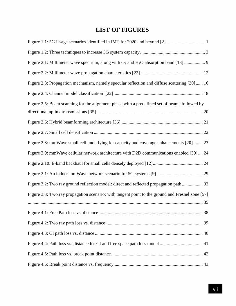
LIST OF FIGURES
Figure 1.1: 5G Usage scenarios identified in IMT for 2020 and beyond [2].................................. 1
Figure 1.2: Three techniques to increase 5G system capacity ........................................................ 3
Figure 2.1: Millimeter wave spectrum, along with O2 and H2O absorption band [18] .................. 9
Figure 2.2: Millimeter wave propagation characteristics [22] ...................................................... 12
Figure 2.3: Propagation mechanism, namely specular reflection and diffuse scattering [30] ...... 16
Figure 2.4: Channel model classification [22] ............................................................................. 18
Figure 2.5: Beam scanning for the alignment phase with a predefined set of beams followed by
directional uplink transmissions [35] ............................................................................................ 20
Figure 2.6: Hybrid beamforming architecture [36] ....................................................................... 21
Figure 2.7: Small cell densification .............................................................................................. 22
Figure 2.8: mmWave small cell underlying for capacity and coverage enhancements [20] ........ 23
Figure 2.9: mmWave cellular network architecture with D2D communications enabled [39] .... 24
Figure 2.10: E-band backhaul for small cells densely deployed [12] ........................................... 24
Figure 3.1: An indoor mmWave network scenario for 5G systems [9] ........................................ 29
Figure 3.2: Two ray ground reflection model: direct and reflected propagation path .................. 33
Figure 3.3: Two ray propagation scenario: with tangent point to the ground and Fresnel zone [57]
....................................................................................................................................................... 35
Figure 4.1: Free Path loss vs. distance .......................................................................................... 38
Figure 4.2: Two ray path loss vs. distance .................................................................................... 39
Figure 4.3: CI path loss vs. distance ............................................................................................. 40
Figure 4.4: Path loss vs. distance for CI and free space path loss model ..................................... 41
Figure 4.5: Path loss vs. break point distance ............................................................................... 42
Figure 4.6: Break point distance vs. frequency ............................................................................. 43
viii
Figure 4.7: Directional PDP at 38 GHz for both LOS and NLOS environment with 2x2 antenna
configuration ................................................................................................................................. 44
Figure 4.8: Directional PDP at 73 GHz for both LOS and NLOS environment with 2x2 antenna
configuration ................................................................................................................................. 46
Figure 4.9: Directional power delay profile at 38 GHz for both LOS and NLOS environment
with 64x16 antenna configuration ................................................................................................ 47
Figure 4.10: Directional power delay profile at 73 GHz for both LOS and NLOS environment
with 64x16 antenna configuration ................................................................................................ 48

ix
LIST OF ABBREVIATIONS
3GPP 3rd Generation Partnership Project
4G Fourth Generation
5G Fifth Generation
ABG Alpha Beta Gamma
AoA Angle of Arrival
AoD Angle of Departure
AR Augmented Reality
BSs Base Stations
CI Close In
D2D Device to Device
DL Down Link
EHF Extremely High Frequency
eMBB enhanced Mobile Broad Band
FCC Federal communication commission
FI Floating Intercept
FSL Free Space Loss
H2O Water
HetNets Heterogeneous Networks
HPBW Half Power Beam Width
IEEE Institute of Electrical and Electronic Engineering
IMT International Mobile Telecommunication
IOT Internet of Thing
x
ITU International Telecommunication Union
LOS Line of Sight
MATLAB Matrix Laboratory
METIS Mobile and wireless communications Enablers for the Twenty-
twenty Information Society
MiWEBA Millimeter-Wave Evolution for Backhaul and Access
M-MIMO Massive Multiple Input Multiple Output
MMSE Minimum Mean Square Error
mMTCs massive Machine Type Communications
mmWave millimeter Wave
MPCs Multi Path Components
NLOS Non Line of Sight
O2 Oxygen
PLE Path Loss Exponent
QoS Quality of Service
QuaDRiGa Quasi Deterministic Radio Channel Generator
RF Radio Frequency
RX Receiver
SLs Spatial Lobes
SSCM Statistical Spatial Channel Model
SUI Stanford University Interim
TCs Time Clusters
TDD Time Division Duplex
xi
TX Transmitter
UDNs Ultra Dense Networks
UE User Equipment
UHD Ultra High Definition
UL Up Link
ULA Uniform Linear Array
UMi Urban Micro
URLLCs Ultra Reliable Low Latency Communications
V2V Vehicular-to-Vehicular
VR Virtual Reality
Wi-Fi Wireless Fidelity
WLAN Wireless Local Network
WPAN Wireless Personal Area Network

xii
ABSTRACT
Existing wireless communications in the sub-6 GHz bands are facing challenges from the growing
demand for higher data rates and better quality of services. To satisfy these demands, the fifth
generation (5G) mobile network would consider unused spectrum in the millimeter wave
(mmWave) spectrum (30-300 GHz). The shortage of bandwidth in the sub-6 GHz band is solved
using mmWave technology. Furthermore, mmWave provides significantly higher throughput, data
rate, and capacity. Despite the fact that a huge bandwidth is employed, mmWave technology
suffers from path loss, atmospheric attenuation, building penetration loss, diffuse scattering from
rough materials, shadowing, and reflection loss. These leads to a decrease in the transmitted
signal power. Therefore, an accurate and reliable channel model is important in the mmWave
bands, particularly for the indoor environment. Moreover, by using technologies like beam-
forming and others coupled with mmWave, the listed impairments are minimized. In this thesis, we
analyze the performance of different path loss models (CI, free space, and two rays) at 38, 60, and
73 GHz carrier frequencies in terms of path loss with respect to the separation distance between
transmitter and receiver. Additionally, we have evaluated the performance of the path loss with
respect to the break point distance to enhance the received signal power and throughput. We have
also done analysis of the directional power delay profile with received signal power, path loss and
path loss exponent (PLE) at 38 GHz and 73 GHz mmWave bands for both LOS and NLOS by using
uniform linear array (ULA) 2X2 and 64x16 antenna configurations using the channel model
simulator (NYUSIM). The simulation results show the performance of different path loss models
in the mmWave and sub 6 GHz bands. The path loss in the close-in (CI) model at mmWave bands
is larger than that of free space and two ray path loss models, because it considers all shadowing
and reflection effects between transmitter and receiver. Moreover, we have scaled up the received
signal power and throughput of mmWave systems by using a large number of antennas at the
transmitter.
Key words: 5G, mmWave, indoor environment, propagation characteristics, path loss, break point
distance

1
CHAPTER ONE
1 INTRODUCTION
1.1 Background
Wireless communications have progressed, and mobile data traffic is predicted to expand by 1000-
fold over the next decade. The growing number of connected devices, the tremendous growth of
mobile services and customer demands will put a tremendous strain on the existing wireless
communication infrastructure. To address these concerns, the wireless industry is moving toward
5G cellular technology, which will boost capacity while also improving energy efficiency, cost,
and spectrum use [1].
Mobile broadband has always been a key in the advancement of mobile communication systems,
hence it is the main driving force behind 5G. Future 5G systems, on the other hand, are predicted
to have a significantly larger societal influence than the previous system. As a result, they will
focus on a wide range of use cases as specified in the 5G plan by ITU for 2020 and beyond. As
indicated in figure 1.1, these use cases include eMBB, mMTCs, and URLLCs.
Figure 1.1: 5G Usage scenarios identified in IMT for 2020 and beyond [2]

2
The eMBB use case is characterized by broadband data access everywhere, from sparsely-
populated areas to densely-populated areas, like indoor hotspots, stadiums, venues, and high-speed
public transportation networks. The goal is to give the best possible user experience by enabling
indoor and outdoor connectivity and providing high QoS internet even in difficult network
situations. The other applications supported by this use case are AR, VR, and context recognition.
The mMTC use case's goal is to link everything to the internet. This massive connectivity will
improve infrastructure automation and monitoring, allowing them to operate with little to no
human interaction. As a result, mMTC use cases will enable IOT applications like smart homes
and cities, as well as smart agriculture. In addition to these characteristics, mMTC should have a
wide range of coverage and, most crucially, low power consumption and low-cost devices that are
critical for achieving this use case goal.
The URLLC use case is designed for applications requiring very low latency, like remote
healthcare, self-driving or autonomous vehicles, and factory automation. URLLCs are expected to
have high reliability, continual availability, and high security because these applications frequently
entail individual or public safety.
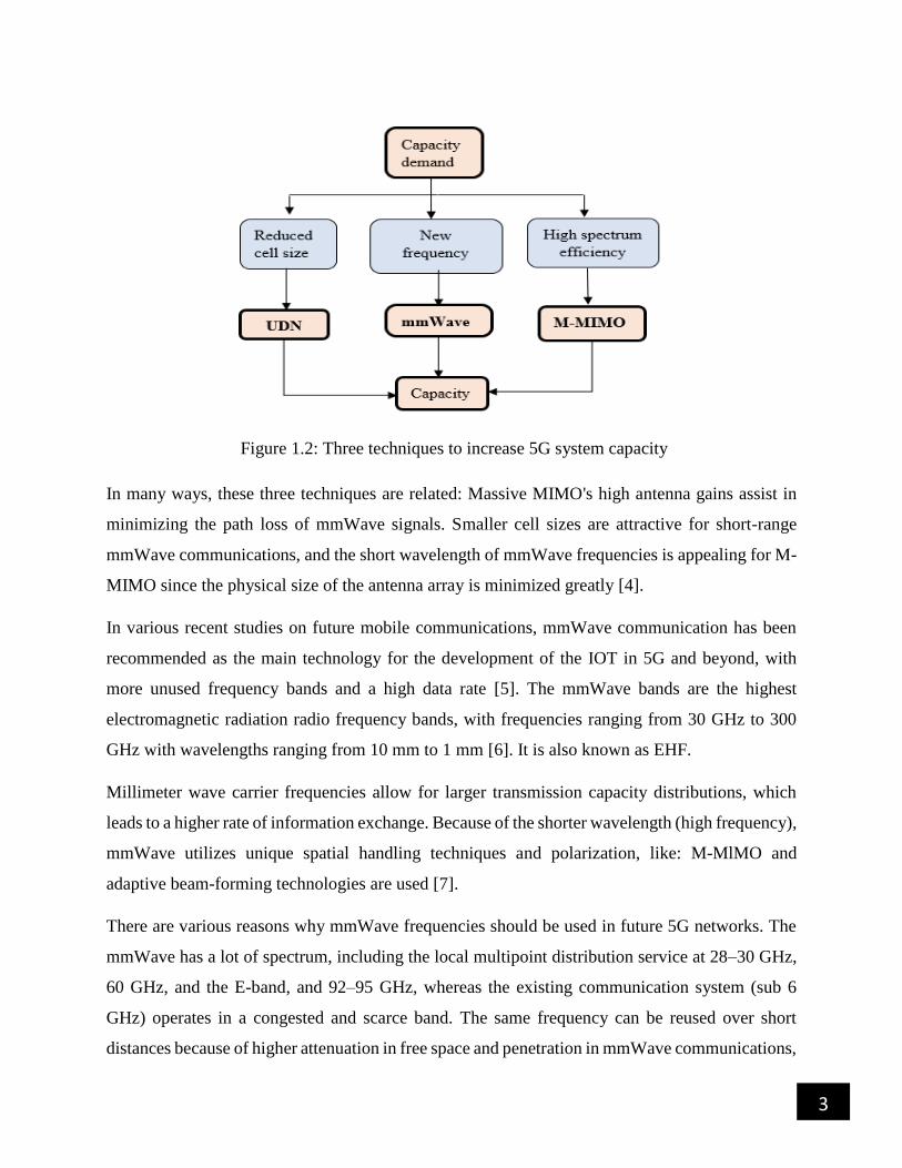
To achieve the 5G design targets, many technologies have been identified, including mmWave
communications, M-MIMO, small cell deployment, full duplex relaying, and D2D
communications. However, the information theory says three of the listed technologies highly
achieve multiple orders of magnitude increases in system capacity: (i) UDNs: existing 4G wireless
cellular networks have already embraced network densification, which is known as small cell
technology, and a denser network can further enhance network capacity; (ii) Large amounts of
bandwidth: moving to higher frequencies will offer a large quantity of bandwidth that can be used
to increase capacity. mmWave communications, in particular, could be a promising candidate,
with carrier frequencies ranging from 30 to 300 GHz; (iii) High spectrum efficiency: by deploying
a large number of antennas at the BS (100 or more), M-MIMO can considerably enhance spectrum
efficiency by utilizing available space resources [3].
3
Figure 1.2: Three techniques to increase 5G system capacity
In many ways, these three techniques are related: Massive MIMO's high antenna gains assist in
minimizing the path loss of mmWave signals. Smaller cell sizes are attractive for short-range
mmWave communications, and the short wavelength of mmWave frequencies is appealing for M-
MIMO since the physical size of the antenna array is minimized greatly [4].
In various recent studies on future mobile communications, mmWave communication has been
recommended as the main technology for the development of the IOT in 5G and beyond, with
more unused frequency bands and a high data rate [5]. The mmWave bands are the highest
electromagnetic radiation radio frequency bands, with frequencies ranging from 30 GHz to 300
GHz with wavelengths ranging from 10 mm to 1 mm [6]. It is also known as EHF.
Millimeter wave carrier frequencies allow for larger transmission capacity distributions, which
leads to a higher rate of information exchange. Because of the shorter wavelength (high frequency),
mmWave utilizes unique spatial handling techniques and polarization, like: M-MlMO and
adaptive beam-forming technologies are used [7].
There are various reasons why mmWave frequencies should be used in future 5G networks. The
mmWave has a lot of spectrum, including the local multipoint distribution service at 28–30 GHz,
60 GHz, and the E-band, and 92–95 GHz, whereas the existing communication system (sub 6
GHz) operates in a congested and scarce band. The same frequency can be reused over short
distances because of higher attenuation in free space and penetration in mmWave communications,
4
which allows high throughput networks. At mmWave frequencies, antennas are so small in size
that complicated antenna arrays and further integration onto chips or PCBs are possible. Due to
the short range of transmission and narrow beam-width, the inherent security and privacy of
mmWave communication is enhanced [8]. Therefore, we implement this technology for both the
indoor and outdoor environment.
According to a recent study, 80 percent of wireless traffic will originate from indoor environments
in the coming years. As a result, mmWave technology must be used to handle the massive data
demand in the indoor environment. Generally, indoor communication originates in a LOS scenario,
however, when the network becomes more congested, a NLOS scenario may occur. Therefore, the
current 4G network is unable to handle the growing demand for data indoors due to its limited
spectrum of microwave frequencies. Hence, 5G with mmWave could be a viable option for indoor
networks [9]. But, when deploying mmWave in an indoor environment, understanding the
propagation characteristics and channel impediments are important. The main impairments of
mmWave propagation are path loss, reflection loss, and increased blocking effects because of
weaker NLOS paths due to the availability of buildings, which are often made of concrete, bricks,
glass, wood, and other home materials, as well as human. Moreover, the noise power is high
because of the use of higher bandwidth [10].
Besides the listed impediments, attenuation is induced by absorption of air molecules, mainly O2
and H2O, which disturbs mmWave communication more significantly than microwave
frequencies. But, for cells with a radius of less than 200 m, atmospheric absorption as well as rain
attenuation do not result in extra path loss [9]. Despite suffering from the listed impairments,
mmWave provides a huge bandwidth for short-range transmission, making it a preferable option
for indoor wireless communication.
In this thesis, we considered different path loss models for the indoor environment at different
carrier frequencies (38, 60, and 73 GHz). We chose these frequencies because most of the current
research in mmWave focuses on the 28 GHz, 38 GHz, V band (60 GHz) and E band. We improved
the received signal power and throughput by analyzing path loss in several path loss models with
a distance between TX and RX and the path loss with break point distance for different heights of
transmitter using MATLAB. We also compared the directional power delay profile with received
signal power, path loss and path loss exponent (PLE) at 38 GHz and 73 GHz mmWave bands for
5
both LOS and NLOS by using ULA 2X2 and 64x16 antenna configurations using the MATLAB
based NYUSIM simulator.
1.2 Statement of the Problem
For nearly two decades, the 2.4 GHz and 5 GHz industrial Wi-Fi frequency bands have been
utilized for short-range indoor wireless communications in offices, conference halls, hotels, and
restaurants [11].
Due to the fact that people spend the majority of their time at home and at work, the majority of
voice and multimedia services take place in an indoor environment. As a result, the capacity
demand for indoor communications will continue to rise at an alarming rate, not handled by the
current Wi-Fi radio band. In order to support the massive data flow, these situations require the
use of more advanced indoor communication networks. The vast amount of unused frequency
resources in the mmWave spectrum is being considered as one of the primary solutions to wireless
network congestion. Hence, the frequency band in mmWave offers higher bandwidths for indoor
wireless communication systems.
As a result, research has focused on the mmWave spectrum. However, because of its short
wavelength, the mmWave travels and propagates through LOS communication, which means that
physical objects like buildings, walls, humans, and home furniture can stop and affect these waves,
in turn reducing the received signal power and throughput, especially in indoor communication.
Recent studies have demonstrated that for small cell sizes on the order of 200 m and by
implementing technologies such as Massive MIMO, Beam-forming, and directional antennas, the
issues mentioned above can be minimized [12].
1.3 Objectives
1.3.1 General objective
The main objective of this thesis is to analyze the performance of mmWave communication using
different path loss models to enhance the received signal power and throughput in an indoor
environment.
1.3.2 Specific objectives
To compare path loss at sub 6 GHz and mmWave frequencies.
To evaluate the path loss of a two-ray model at different frequencies.

6
Compare different path loss models at mmWave frequencies.
To analyze path loss model with different first Fresnel zone break points.
To analyze Fresnel zone break points with different mmWave frequencies.
To compare the received signal power in LOS and NLOS scenarios at mmWave
frequencies using different antenna configurations.
1.4 Significance
This work improves the received power of a communication system by minimizing the path loss
effect. Hence, in this thesis we examined the path loss with different separation between TX-RX
and breakpoint distances for different path loss models at different carrier frequencies, particularly
for the indoor environment. There are many obstacles in this environment, such as home furniture,
human beings, and ground reflection, that cause the transmitted signal to propagate in different
directions, causing blockage and path loss, which reduces the received signal power and also
throughput. As a result, path loss and blockage effects must be minimized. To minimize these
problems, a large number of antennas are being considered.
1.5 Scope
This thesis focuses on enhancing the received signal power and throughput in an indoor
communication system at different mmWave frequencies (38, 60, and 73 GHz) by analyzing the
path loss at different separation distances and breakpoint distances. In mmWave there are many
unused spectrums available. However, the path loss increases as the carrier frequency increases
(short wavelength), because the signal propagates in different directions with the same or different
time delays and angles due to obstructing objects between the transmitter and receiver whose sizes
are larger than the size of the transmitted signal. As a result, the received signal power and
throughput are reduced. Different path loss models have been proposed by different researchers.
In this thesis, we used free space, two rays, and CI path loss models to analyze the effects of
mmWave indoor communication at 38 GHz, 60 GHz, and 73 GHz carrier frequencies. Moreover,
we compared the directional PDP at 38 and 73 GHz frequencies for both LOS and NLOS scenarios
using ULA 2X2 and 64X16 antenna configurations.

7
1.6 Main contribution
The main contribution of this thesis is to evaluate the performance of mmWave communication
from the perspective of two rays and multipath. Moreover, we have also derived path loss
formulations as a function of break point distance.
1.7 Thesis organization
The rest of the thesis is organized as follows:
Chapter 2: Review of different literature on mmWave, M-MIMO/beam forming and small cell
deployment and the existing works related to mmWave radio propagation in an indoor
environment at different path loss models.
Chapter 3: System model and mathematical formulation for the indoor environment at different
carrier frequencies by considering different path loss models.
Chapter 4: Simulation results and discussion of each of the results obtained.
Chapter 5: Conclusions and recommendations for future work.

8
CHAPTER TWO
2 LITERATURE REVIEW
2.1 Introduction to mmWave
The significant technological improvements in mobile and wireless communications systems have
not kept pace with current spectrum availability for cellular networks throughout the years. The
frequency ranges below 6 GHz are used by almost all mobile and wireless technologies. Hence,
the frequency available in the sub–6 GHz band will be insufficient to supply the required capacity
for future communication networks [13]. As a result, shift to the mmWave frequency bands, which
offer wider bandwidths.
The mmWave spectrum is a band of the spectrum that spans from 30 GHz to 300 GHz and
corresponds to wavelengths of 10 mm to 1 mm, which is between microwave and infrared.
However, in the wireless sector, the frequency ranges beyond 6 GHz are referred to as the
mmWave bands. Standard organizations, the FCC, and researchers are considering it as a means
of bringing "5G" into the future by assigning larger bandwidth to enable faster, higher-quality
video and multimedia content and services [14].
Since the first mmWave communications were demonstrated over a century ago, mmWave
frequencies have been used in several applications, including radar remote sensing, satellite
communications, and security systems to improve precision and resolution [15]. However, because
of the harsh propagation constraints involved in mmWave communications, like shadowing, larger
Doppler spreads, high penetration loss, and high air absorption, particularly for NLOS channels,
mmWave technology is not used for terrestrial mobile applications [16].
Despite the propagation constraints, mmWave frequencies remain highly attractive for future
cellular networks, especially for higher-output local area networks as well as personal area
networks. Several recent studies have demonstrated multi-Gbps access communications using
mmWave. The large bandwidth available at mmWave, coupled with various technologies,
including beamforming, small cells, and M-MIMO, make the mmWave an attractive solution for
dense networks and densely populated areas, particularly in an indoor environment [17].
9
2.1.1 Millimeter wave spectrum
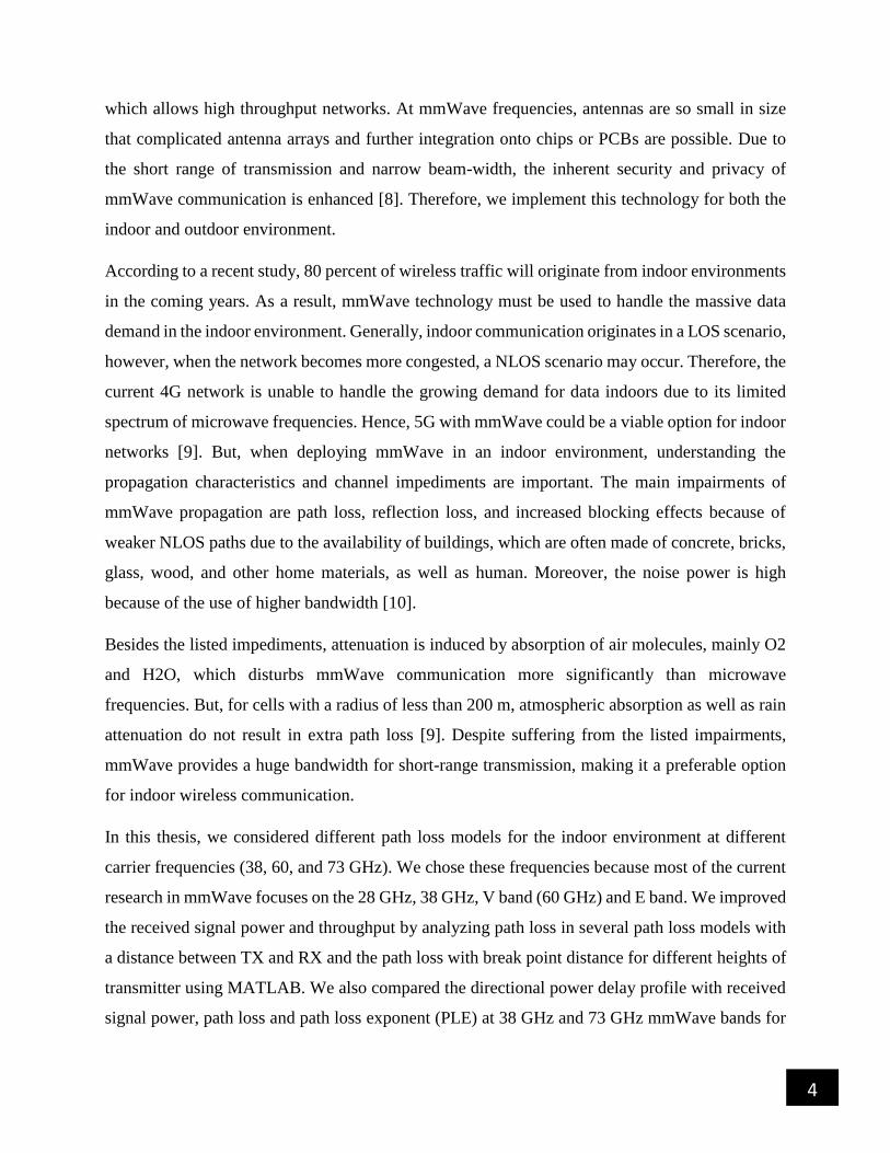
When compared to the microwave, mmWave has a much larger frequency band (30-300 GHz).
Despite the fact that some unfavorable bands, such as 57–64 GHz and 164–200 GHz, as shown in
figure 2.1, are easily absorbed by O2 and H2O respectively, the appropriate bands for mmWave
communications are still above 150 GHz, and more than 150 Gb/s can be attained across the entire
range.
Figure 2.1: Millimeter wave spectrum, along with O2 and H2O absorption band [18]
The mmWave spectrum is divided and named into several bands with related frequency ranges
and wave lengths, as shown in table 2.1. Some applications have been considered for some of these
bands. Satellite communications, astronomy, and terrestrial microwave communications all use
the Q band, which ranges from 30 GHz to 50 GHz. 60 GHz is a portion of the V band that runs
from 50 to 75 GHz. It is used for unlicensed wireless communications and is best for high-speed
indoor communications and short-range high-resolution radar sensors due to its high O2
absorption. In fronthaul and backhaul networks, portions of the E band, including 71 GHz to 76
GHz, 81 GHz to 86 GHz, and 92 GHz to 96 GHz, are used. Satellite communications and deep
space research can both benefit from the W band, which has a short wavelength.
10
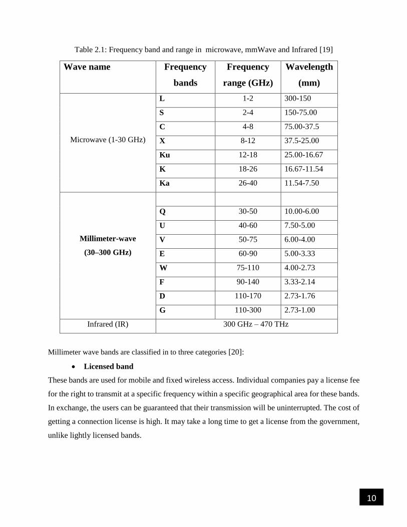
Table 2.1: Frequency band and range in microwave, mmWave and Infrared [19]
Wave name Frequency
bands
Frequency
range (GHz)
Wavelength
(mm)
Microwave (1-30 GHz)
L 1-2 300-150
S 2-4 150-75.00
C 4-8 75.00-37.5
X 8-12 37.5-25.00
Ku 12-18 25.00-16.67
K 18-26 16.67-11.54
Ka 26-40 11.54-7.50
Millimeter-wave
(30–300 GHz)
Q 30-50 10.00-6.00
U 40-60 7.50-5.00
V 50-75 6.00-4.00
E 60-90 5.00-3.33
W 75-110 4.00-2.73
F 90-140 3.33-2.14
D 110-170 2.73-1.76
G 110-300 2.73-1.00
Infrared (IR) 300 GHz – 470 THz
Millimeter wave bands are classified in to three categories [20]:
Licensed band
These bands are used for mobile and fixed wireless access. Individual companies pay a license fee
for the right to transmit at a specific frequency within a specific geographical area for these bands.
In exchange, the users can be guaranteed that their transmission will be uninterrupted. The cost of
getting a connection license is high. It may take a long time to get a license from the government,
unlike lightly licensed bands.

11
.Lightly Licensed band
These bands require a license from the FCC, which can be obtained through performing frequency
coordination, issuing of a public notice, and submission of an application. This procedure ensures
nobody else is utilizing the same or a frequency that will interfere with current systems. The cost
of obtaining a connection license is low, and it may be done in a couple of weeks. Microwave link
operators with a light license are granted exclusive usage of a portion of the band in a specific
direction across a defined geographic area. When licensed radios experience interference, the
problem is usually rectified with the help of the regulating agency. The millimeter bands 11, 13,
18, 23 GHz, and (70/80 GHz) are lightly licensed bands and are mainly used for point-to-point
backhaul.
Unlicensed band
Unlike lightly licensed and licensed bands, it does not require a government license. It is available
without charge. The 60 GHz (V band) is a license-free frequency that can be utilized for point-to-
point and point-to-multipoint backhaul as well as wireless access. The frequency distribution of
the V band varies by country. In the United States, it consists of 14 GHz (57-71 GHz). This is 15
times more than the total amount of unlicensed Wi-Fi spectrum in the lower bands. Whereas, in
Europe, it is 9 GHz (57-66 GHz).
2.1.2 Opportunities in mmWave
Besides the larger amount of bandwidth, mmWave has a number of advantages over conventional
radio waves. These are:
Larger Antenna Array
Because of the short wavelengths of mmWave communications, a large number of antennas can
be utilized in a small space. This has important implications for antenna systems, as low-cost
fabrication technology and compact integration allow for cost savings and production scale. At the
same time, the beam-width narrows when there are multiple antenna elements. The benefits of this
characteristics include increased security and greater resistance to co-user interference [18].
Channel Reciprocity
Because the frequency bands for mmWave communication are unpaired, it uses a TDD scheme,
which means that DL and UL communications use the same frequency but at different times. The
UL and DL propagation channel characteristics are closely associated in these systems when the
12
DL and UL communications are conducted at a specified period of time, called the channel
coherence time. This process is known as channel reciprocity [20].
Densification
When mmWave coverage is desired in a particular area, a higher density of mmWave cells is
expected than sub-6 GHz cells are employed to achieve the desired coverage. The mmWave band
can give faster data speeds and capacity while still providing enough coverage due to its higher
cell density [20].
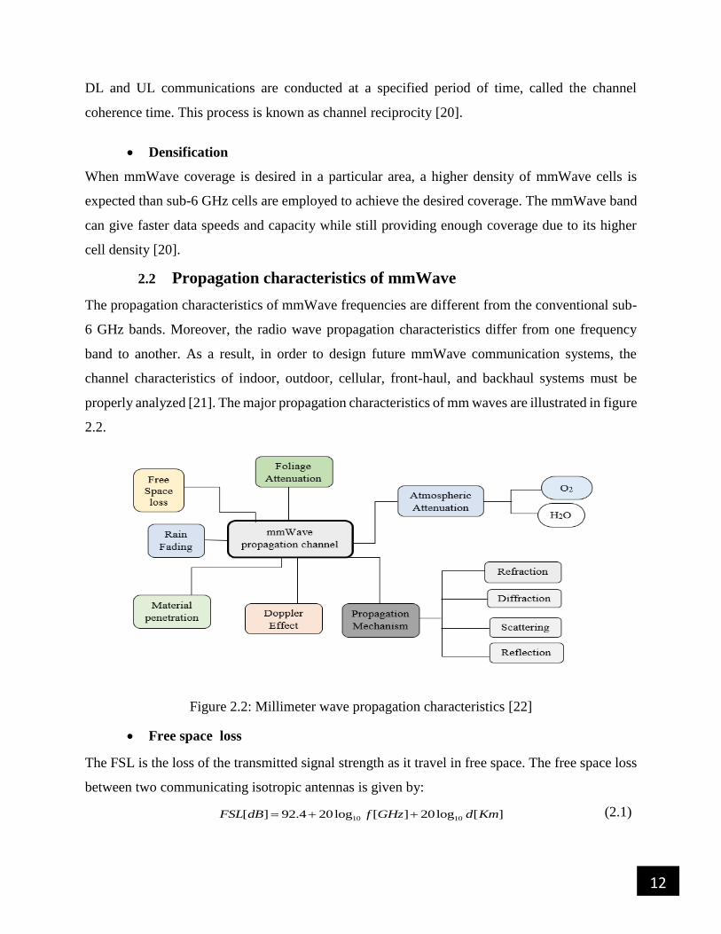
2.2 Propagation characteristics of mmWave
The propagation characteristics of mmWave frequencies are different from the conventional sub-
6 GHz bands. Moreover, the radio wave propagation characteristics differ from one frequency
band to another. As a result, in order to design future mmWave communication systems, the
channel characteristics of indoor, outdoor, cellular, front-haul, and backhaul systems must be
properly analyzed [21]. The major propagation characteristics of mm waves are illustrated in figure
2.2.
Figure 2.2: Millimeter wave propagation characteristics [22]
Free space loss
The FSL is the loss of the transmitted signal strength as it travel in free space. The free space loss
between two communicating isotropic antennas is given by:
10 10[ ] 92.4 20log [ ] 20log [ ]FSL dB f GHz d Km (2.1)
13
Where d is separation distance between transmitter and receiver in kilometers (km) and f is
operating frequency in GHz.
The FSL has a linear relationship to both the separation distance and the carrier frequency,
according to the given equation. When a carrier frequency moves into the mmWave frequency
bands, the FSL increases rapidly in comparison to the sub-6 GHz band.
Atmospheric attenuation
When molecules absorb a portion of the power carried by propagating waves and vibrate according
to the carrier frequency, atmospheric attenuation, also known as gaseous attenuation, occurs. O2
and H2O are the two main absorbing gases at mmWave frequencies. The densities of gaseous
absorption depend on several factors, including temperature, pressure, altitude, and, most
significantly, the operational carrier frequency.
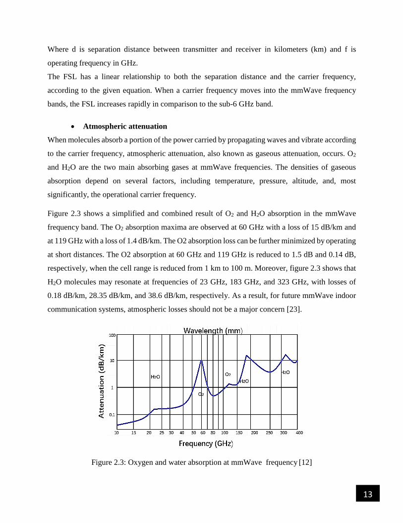
Figure 2.3 shows a simplified and combined result of O2 and H2O absorption in the mmWave
frequency band. The O2 absorption maxima are observed at 60 GHz with a loss of 15 dB/km and
at 119 GHz with a loss of 1.4 dB/km. The O2 absorption loss can be further minimized by operating
at short distances. The O2 absorption at 60 GHz and 119 GHz is reduced to 1.5 dB and 0.14 dB,
respectively, when the cell range is reduced from 1 km to 100 m. Moreover, figure 2.3 shows that
H2O molecules may resonate at frequencies of 23 GHz, 183 GHz, and 323 GHz, with losses of
0.18 dB/km, 28.35 dB/km, and 38.6 dB/km, respectively. As a result, for future mmWave indoor
communication systems, atmospheric losses should not be a major concern [23].
Figure 2.3: Oxygen and water absorption at mmWave frequency [12]
14
Rain attenuation
The precipitation attenuation and losses due to rain are considerable for mmWave. At mmWave
frequencies, raindrops and the size of the transmitted signal wavelengths are nearly the same. As
a result, raindrops easily block mmWave communications, causing the signal's energy to be
scattered and its strength to be lost [24].
The rain attenuation in mmWave and targeted sub-100 GHz bands for 5G is more problematic than
rain attenuation in conventional microwave networks, with a maximum attenuation of nearly 30
dB/km for very heavy rainfall (100 mm/h). Moreover, it has different effects depending on the
mmWave frequency ranges. The path loss due to rain attenuation is not considerable for a short
range of communication on the order of 200 m. Therefore, higher mmWave frequencies are used
in indoor environments and dense urban environments with cell sizes of less than 200 m [25].
Foliage loss
Foliage attenuation is an important attenuating factor in mmWave communications. The existence
of vegetation between the TX and RX induces extra signal loss, which can negatively affect the
QoS of a wireless communication system. The depth of the vegetation component determines the
intensity of foliage attenuation. A single tree has a smaller influence than numerous trees.
Furthermore, radio signals are attenuated more severely by a forest than by several trees [26].
Material penetration
The mmWave frequencies are susceptible to penetration loss, and in comparison to sub-6 GHz, they
can’t penetrate most solid materials well, including walls, doors, and room furniture. As a result,
mmWave communications are easily blocked, particularly in densely urban areas with many buildings
and a large number of people [22]. The mmWave signal's frequency, antenna polarization, angle of
incidence, surface roughness, permittivity of material, and thickness of material all have an impact
on penetration loss [27].
When mmWave signals travel from indoors to outdoors, the penetration loss is roughly 74 dB
because of the inability of these signals to penetrate building materials. Similarly, high penetration
loss has occurred when mmWave signals travel from outdoors to indoors. Therefore, these
propagations may experience a large penetration loss, reducing the data throughput, spectrum
efficiency, and energy efficiency. As a result, the majority of BSs will not be able to provide indoor
15
mmWave coverage. Hence, to achieve indoor-to-outdoor coverage and vice versa, heterogeneous
networks, repeaters, and relays are required [27].
Doppler spread
The Doppler shift occurs when the frequency of a wave changes as the receiver moves away from
and towards the BS. When the transmitter and receiver are moving towards each other, the Doppler
shift is positive (higher frequency), but when they are moving apart from each other, it can be
negative (lower frequency). The Doppler shift is given by [28]:
*
*cosof
f vD
c (2.2)
Where v is relative velocity of the transmitter and receiver, of is the carrier frequency, c is speed
of light in air (3*10^8 m/s), and is an angle that related to the direction of travel.
The Doppler spread is the range shifting up to the maximum and down to the minimum. Which is
obtained from maximum Doppler shift. The maximum Doppler shift is:
maxf c
vD f
c (2.3)
Then Doppler spread becomes:
max
12*d f
c
B DT
(2.4)
Where cT coherent time of a channel and maxfD maximum Doppler shift.
According to the equation, the coherent time of a channel and frequency have an inverse
relationship for a given user mobility, hence it is very small in the mmWave band, resulting in
rapid channel fluctuations and inconsistent connectivity. According to some studies, at 60 km/h
and 60 GHz, the Doppler spread is above 3 kHz, implying that the channel will shift on the order
of hundreds of microseconds, much faster than current cellular systems [29].
Human blockage
Because humans operate as the greatest barriers, reflectors, and scatters, their presence has a
serious effect on the propagation characteristics of mmWave signals. The reason behind this
problem is that the size of the human body is quite large in comparison to the mmWave signal.
16
Furthermore, when mmWave comes into contact with the human body, it experiences low
penetration loss, whereas reflection and scattering, result in high losses.
Propagation mechanism
The major causes of NLOS propagation between TX and RX are refraction, diffraction, and
scattering. In this scenario, the transmitted signals still reach the receiver due to reflections from
nearby objects, bending, or diffraction. Reflection and scattering occur when the barriers between
TX and RX are larger than the propagating signal's wave length. As a result, short-wavelength
mmWave signals are subjected to more shadowing and reflection and less diffraction [30].
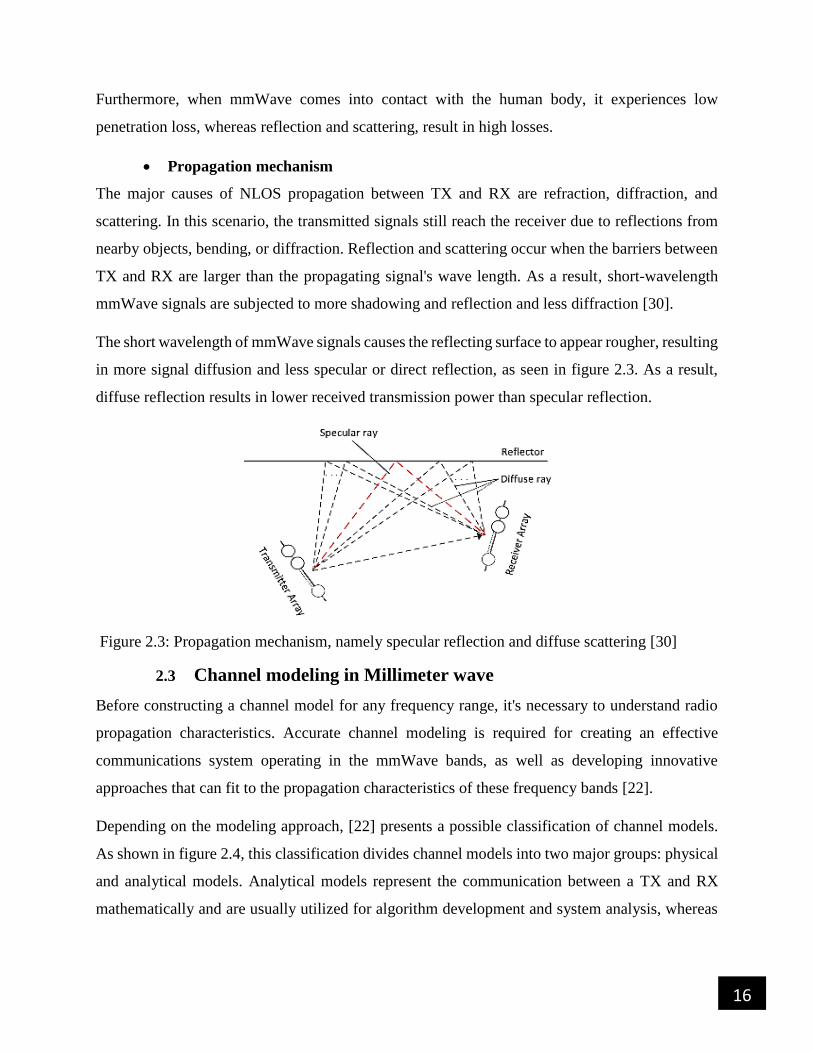
The short wavelength of mmWave signals causes the reflecting surface to appear rougher, resulting
in more signal diffusion and less specular or direct reflection, as seen in figure 2.3. As a result,
diffuse reflection results in lower received transmission power than specular reflection.
Figure 2.3: Propagation mechanism, namely specular reflection and diffuse scattering [30]
2.3 Channel modeling in Millimeter wave
Before constructing a channel model for any frequency range, it's necessary to understand radio
propagation characteristics. Accurate channel modeling is required for creating an effective
communications system operating in the mmWave bands, as well as developing innovative
approaches that can fit to the propagation characteristics of these frequency bands [22].
Depending on the modeling approach, [22] presents a possible classification of channel models.
As shown in figure 2.4, this classification divides channel models into two major groups: physical
and analytical models. Analytical models represent the communication between a TX and RX
mathematically and are usually utilized for algorithm development and system analysis, whereas

17
physical models use electromagnetic characteristics to represent communication and can
realistically reproduce channel characteristics depending on the complexity.
Physical channel models are further classified into two, as shown in figure 2.4, stochastic and
deterministic models. Deterministic models are well-known for their accuracy in forecasting
channel properties in a deterministic manner, but they come at a high cost in terms of computation
and modeling complexity. These models are utilized when the propagation environment is known
and they are particularly specific to that environment. Ray-tracing, in which each multipath
component is represented as a ray, is the most extensively used technique in deterministic models.
Ray tracing is often done with a standalone software program to simulate a desired channel
situation with all known environmental conditions and kept in the system. Another benefit of
deterministic models, particularly ray tracing models, is that they may be quickly used to predict
the features of a new environment if no measurements for that situation are available. This saves
a lot of money on measuring campaigns.
The Stochastic channel models, on the other hand, generate the channel's impulse response, which
describes the spatio-temporal properties of the channel's MPCs based on the measurements taken
in various situations and conditions. Large-scale and small-scale fading characteristics are
commonly described using PDFs of channel parameters. These channel models are simple models
which take a short time and have reduced complexity in computational, making them suitable for
systems design and simulation.

18
Figure 2.4: Channel model classification [22]
2.3.1 Current channel model in Millimeter Wave
METIS: developed the mmWave channel model based on measurements taken in various
situations at various frequencies that are not sufficiently represented by existing channel models.
The METIS project suggested three channel models, such as stochastic, map-based, and hybrid
(which is a combination of the two models) to meet the needs for flexibility and scalability. The
stochastic model is appropriate for frequencies up to 70 GHz, whereas the map-based model is
appropriate for frequencies up to 100 GHz. In these models, ray-tracing techniques and
measurement-based results are used to generate large-scale and small-scale fading characteristics,
respectively. The project includes different propagation environments, including indoor office,
urban micro-cell, urban macro-cell, D2D, V2V, and rural macro-cell [31].
MiWEBA: developed to characterize the 60-GHz outdoor multipath channels, is characterized by
the superposition of a few strong deterministic pathways and numerous very weak random rays,
which use a quasi-deterministic channel model. MiWEBA is capable of supporting mmWave
massive MIMO communications and beamforming. This channel model is applicable only to the
specific situation under consideration and can't be applied to other situations because the quasi-
deterministic modeling technique requires a precise description of the situation [32].
QuaDRiGa: is a 3D geometry-based stochastic channel model which was created primarily for
modeling MIMO channels in specific network configurations. QuaDRiGa supports the mmWave

19
spectrum from 0.45 GHz to 100 GHz, with a bandwidth of up to 1 GHz, and provides spatial
consistency primarily through the correlation of large-scale and small-scale characteristics. This
channel model incorporates the characteristics of the 3GPP spatial channel model extension and
WINNER channel models, and also new modeling techniques, to provide quasi-deterministic
receiver-movement-multi-link tracking in changing situations [33].
The 3GPP Model: is a recently suggested 3D representation of the 3GPP channel model,
specifically the 3GPP TR 38.900 3D model, which is an expansion of the 3GPP TR 36.873
channel, which is typically utilized for sub-6 GHz. The current model supports frequency bands
up to 100 GHz in a variety of scenarios, including urban macro cells, urban micro cells, D2D,
indoors, and so on. In addition to the azimuth angle dimension, this 3D model can also capture the
channel's elevation angle dimension.
NYUSIM: a MATLAB-based-open source channel model simulator created by NYU
WIRELESS. NYU WIRELESS is an academic research institute focusing on mmWave
technology. It can operate at up to 100 GHz carrier frequency and 800 MHz RF bandwidth. This
simulator employs a SSCM for broadband mmWave wireless communication, which generates
channel responses and accompanying AoA/AoD power spectra using TCs and SLs. Because of the
high gain directional antennas of MIMO, NYUSIM captures multipath components in a TC
method from diverse pointing angles. These characteristics are not taken into account in the
WINNER and 3GPP models. Furthermore, under the 3GPP/WINNER model, the number of
measured path loss samples and their respective distances have a significant impact. NYUSIM, on
the other hand, employs both a close-in distance (CI) parameter and a PLE. As a result, better
stability is achieved in a variety of environmental conditions. Therefore, in comparison to the
3GPP and also other channel models for mmWave bands, it is more realistic [34].
2.4 Beamforming technology
Beamforming enhances the BS antenna gain and helps focus the energy of antennas in a particular
direction while avoiding interference from other sources. When transmit and receive antennas are
used to achieve beamforming gain, the path loss of mmWave transmission can be comparable to
that of a conventional carrier frequency band. The short wavelength, in particular, enables the
construction of arrays of antennas with several other elements in a compact space that can focus
energy in narrow beams in adjustable directions. There are three beamforming techniques: digital,
20
analog, and hybrid. Each of these techniques has a major impact on energy consumption, attainable
beamforming gain, complexity, and runtime [12].
2.4.1 Analog beamforming
Analog beamforming is an effective method of creating high beamforming gain with a large
number of antennas allowed in mmWave bands. All of the antennas share the same radio frequency
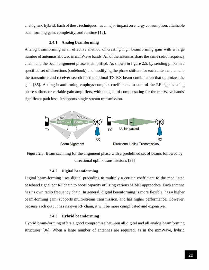
chain, and the beam alignment phase is simplified. As shown in figure 2.5, by sending pilots in a
specified set of directions (codebook) and modifying the phase shifters for each antenna element,
the transmitter and receiver search for the optimal TX-RX beam combination that optimizes the
gain [35]. Analog beamforming employs complex coefficients to control the RF signals using
phase shifters or variable gain amplifiers, with the goal of compensating for the mmWave bands'
significant path loss. It supports single-stream transmission.
Figure 2.5: Beam scanning for the alignment phase with a predefined set of beams followed by
directional uplink transmissions [35]
2.4.2 Digital beamforming
Digital beam-forming uses digital precoding to multiply a certain coefficient to the modulated
baseband signal per RF chain to boost capacity utilizing various MIMO approaches. Each antenna
has its own radio frequency chain. In general, digital beamforming is more flexible, has a higher
beam-forming gain, supports multi-stream transmission, and has higher performance. However,
because each output has its own RF chain, it will be more complicated and expensive.
2.4.3 Hybrid beamforming
Hybrid beam-forming offers a good compromise between all digital and all analog beamforming
structures [36]. When a large number of antennas are required, as in the mmWave, hybrid

21
beamforming is preferable, because it is a trade-off between flexibility/cost, simplicity, and
performance.
A hybrid beamforming architecture is shown in figure 2.6 at both the TX and RX. In this design,
the narrow beams created using analog beamforming (phase shifters) mitigate the significant path
loss at mmWave bands, while digital beamforming gives the flexibility needed to conduct
advanced multi-antenna approaches like multi-beam MIMO.
Figure 2.6: Hybrid beamforming architecture [36]
2.5 Small cell deployment
The mmWave networks can be made very dense to overcome blockages, and can benefit from the
current trend of moving cellular systems to a large number of small–cells, which we call network
densification. The concept of network densification employing small–cells, as shown in figure 2.7,
is easier to construct and more cost-effective because it uses less transmission power and serves a
small number of users. A network including these different cell sizes is called a HetNets. HetNets,
which allow home users to buy small cell BSs and place them in areas with poor reception [37].
Furthermore, because small–cells are placed much closer to the UEs than typical macro–cells,
higher coverage is attained. Small–cell deployment, varying from micro–cells to femto–cells, will
boost the spectrum reuse ratio as cell sizes decrease. As a result, HetNets are predicted to enable
considerable significant improvements in spectral efficiency [38]. HetNets may incorporate other
22
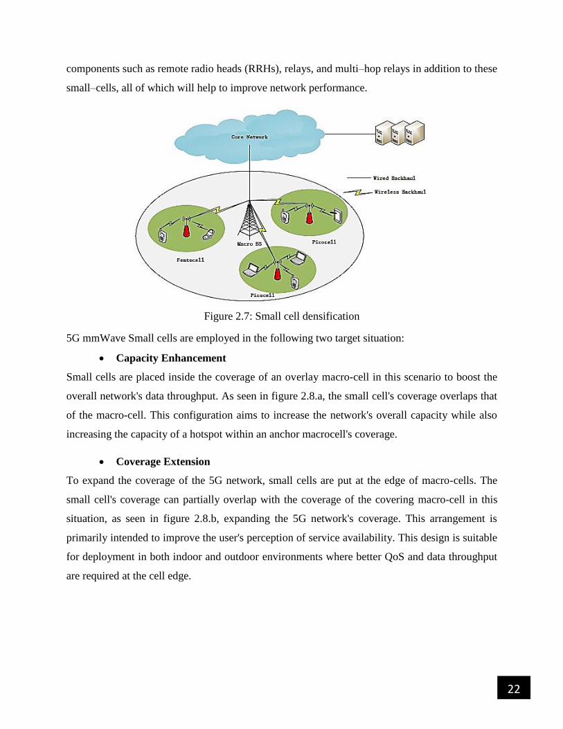
components such as remote radio heads (RRHs), relays, and multi–hop relays in addition to these
small–cells, all of which will help to improve network performance.
Figure 2.7: Small cell densification
5G mmWave Small cells are employed in the following two target situation:
Capacity Enhancement
Small cells are placed inside the coverage of an overlay macro-cell in this scenario to boost the
overall network's data throughput. As seen in figure 2.8.a, the small cell's coverage overlaps that
of the macro-cell. This configuration aims to increase the network's overall capacity while also
increasing the capacity of a hotspot within an anchor macrocell's coverage.
Coverage Extension
To expand the coverage of the 5G network, small cells are put at the edge of macro-cells. The
small cell's coverage can partially overlap with the coverage of the covering macro-cell in this
situation, as seen in figure 2.8.b, expanding the 5G network's coverage. This arrangement is
primarily intended to improve the user's perception of service availability. This design is suitable
for deployment in both indoor and outdoor environments where better QoS and data throughput
are required at the cell edge.

23
Figure 2.8: mmWave small cell underlying for capacity and coverage enhancements [20]
2.6 Applications of mm Wave communications
Small cell access
Small cells placed as WLANs or WPANs beneath macro cells are a possible approach to increasing
capacity in 5G cellular networks. mmWave small cells can enable multi-gigabit rates and
wideband multimedia applications due to their large bandwidth [12].
D2D communications
The use of directional antennas in mmWave communication introduces a new characteristic to the
system: narrow directed beams that minimize fading, multipath, and interference. The mmWave
devices can operate more effectively in noise-limited rather than interference-limited situations
because adaptive arrays with narrow beams reduce interference. This mmWave feature is used in
device-to-device communications that allows a user equipment to interact directly with another
user equipment in close proximity over a D2D link without having to go through the central BS.
The mmWave 5G cellular network design with device-to-device communications is shown in
figure 2.9. These communications in close proximity reduce power and enhance spectrum
efficiency, hence they should be activated in millimeter wave cellular networks to allow context-
aware applications that need to discover and converse with adjacent devices.

24
Figure 2.9: mmWave cellular network architecture with D2D communications enabled [39]
Wireless backhaul
Fiber-based backhaul is expensive to connect 5G BSs to each other and to the network because
small cells are widely distributed in the next generation of cellular networks. Due to the high
bandwidth available, wireless backhaul in mmWave bands such as the 60 GHz and E-band can
provide multiple gigabit per second data speeds and can be a feasible backhaul solution for small
cells. The E-band backhaul, as indicated in figure 2.10, allows high-speed communication between
small cell BSs or between BSs and the gateway.
Figure 2.10: E-band backhaul for small cells densely deployed [12]

25
2.7 Related works
In [40] for both LOS and NLOS scenarios, the characteristics of mmWave multipath propagation
based on path loss, delay spread, and received power for several mmWave bands at 28, 39, 60, and
73 GHz for indoor communication have been analyzed. They consider the effects of different
building materials, frequency sensitivity materials, and multi-floor indoor communication systems
on signal propagation characteristics. The researchers employed wireless insite software to assess
the performance of each frequency; the results show an inverse relationship between separation
distance, frequency, and both delay spread and received power. Furthermore, path loss increases
as the separation distance and frequency increase for a variety of reasons related to antenna
directionality and characteristics.
In [41], the channel propagation characteristics of a 5G system in LOS and NLOS scenarios are
presented. Based on the data they collected in an indoor environment at 3.5 GHz and 28 GHz, the
diffraction loss (DL) and frequency drop (FD) are evaluated. The parameters for path loss are
determined using several path loss models (CI and ABG) for single and multi-frequencies. The
power delay profile, excess delay, and root mean square (RMS) delay dispersion of received paths
are analyzed. At both frequencies, the PLE in the indoor environment is less than the free space
path loss exponent for the LOS scenario, according to the results of the path loss models. However,
in the NLOS case, where the PLE value is higher than the free space PLE, the received power is
reduced.
In [42], an analytical approach for evaluating the levels of propagation losses experienced by mm-
Wave signals in an indoor environment is presented. The analysis used the free space model, the
ABG Path loss model, the CI model, the SUI Model, and the Ericsson Model. To evaluate the
varying signal path loss, different mmWave frequencies, 28, 38, 60, and 73 GHz, were deployed
with distances ranging from 1 m to 5 m. To determine the varying penetration losses, different
physical propagation mediums were evaluated. The results showed that the ABG propagation
model, which has the lowest penetration loss, is the most suitable for indoor applications, followed
by the CI model. The Ericsson model was characterized as having the highest penetration loss.
The statistical channel modeling for LOS and NLOS scenarios in an indoor environment using the
NYUSIM simulator is presented in [9]. Comparing both directional and omnidirectional PDP with
respect to path loss, received signal power, and PLE for both scenarios using a ULA 4x4 antenna
26
configuration at 60 GHz. The results showed that the received signal power in directional PDP is
better than in omnidirectional PDP for both scenarios.
In [43], a comparison of CI and FI models with single- and multi-frequency path loss models at
28 and 73 GHz in three indoor office designs, including corridor, open-plan, and closed-plan, was
made. The results show that employing single and multi-frequency path loss models with close-in
free space reference distances simplifies path loss calculation and prediction across a wide range
of distances and frequencies. Whereas, the high variances in the FI and ABG model parameters
leads to large inaccuracies.
The mmWave propagation characteristics at 26, 32, and 39 GHz frequency bands in the corridor
indoor scenario with LOS conditions using two antenna configurations are presented in [44]. A
horn antenna was utilized in transmission, while horn and omnidirectional antennas were
employed in reception. The path loss in the horn configuration is higher than in the Omni. On
average, path loss is larger at higher frequencies, as expected. In all cases, the path loss exponents
are less than 2, confirming a waveguide-like propagation effect in LOS conditions.
In [45] at 28 and 73 GHz, mmWave propagation with respect to path loss was examined in an
office environment, for transmit powers of 24 dBm and 12.3 dBm, respectively. PDPs were
obtained for 48 TX-RX position pairs with a distance range from 3.9 to 45.9 m. For both co-and
cross-polarized antenna designs, directional and omnidirectional path loss models, as well as RMS
delay spread, are given for LOS and NLOS conditions. In both LOS and NLOs scenarios,
omnidirectional PLEs are larger than directional PLEs for vertically polarized antennas. They also
used a technique known as beamfoarming at the BS and UE to enhance received signals and
expand coverage by searching for the strongest transmitter-receiver angle directing link at each
receiver position.
The large-scale path loss model for the indoor environment is presented in [46], for 4.5, 28, and
38 GHz bands. The effect of path loss on 5G signals transmitted over these frequency ranges was
analyzed. The CI model is more efficient than the FI model for single-frequency path loss. As a
result, the FI model does not accurately describe the channel in a LOS and NLOS scenario.
Moreover, the multi-frequency ABG path loss model showed that all frequency slope values (γ) in
LOS and NLOS indicate an undesirable level of attenuation as frequency increases.

27
From the reviewed related works, researches were done on different indoor environments using
different path loss models like CI, FI, ABG, and SUI using different antenna configurations for
LOS and NLOS. Unlike these works, this thesis focuses on evaluating the performance of
mmWave communication from the perspective of two rays and multipath. Also, analyzing the path
loss at different separation distances and breakpoint distances for CI, free space and two rays for
different mmWave bands. Additionally, by adding a large number of antennas at the TX and RX
with a co-polarized antenna configuration, the received power of the directional PDP for both LOS
and NLOS scenarios is compared.
28
CHAPTER THREE
3 SYSTEM MODEL
In this thesis, different related literature is reviewed from different journals, IEEE papers, and
books on 5G technologies focusing on mmWave, beam-forming techniques, and propagation
characteristics of mmWave, particularly in an indoor environment. Depending on this literature
and having the statement of the problem, to achieve the desired objectives, the following
methodologies are designed:
1) System models and different mathematical formulations
A Mathematical model for calculating path loss for different path loss models.
A mathematical model for calculating the breakpoint distance from the first Fresnel
zone.
Derive mathematical expressions that relate the path loss to the break point distance.
2) Identify input parameters for the simulation
3) Perform simulation using MATLAB R2015b and NYUSIM simulators
Simulation for path loss analysis of different frequency bands (38, 60, and 73 GHz)
for the indoor environment using different path loss models (free space, CI, and
two rays).
Simulation for path loss analysis of different frequency bands with varying
breakpoint distance.
Simulation for break point distance at different carrier frequencies, transmitter
and receiver height.
Simulation for directional PDP at 38 and 73 GHz using 2x2 and 64x16 antenna
configurations for both LOS and NLOS scenarios.
3.1 System model and Mathematical Formulation
In figure 3.1, a system model for an indoor environment is displayed, with both LOS and NLOS
conditions. In an indoor environment, the microcell's base station provides mmWave access link
connectivity to all UEs and access points. When the environment is clear of obstructions and the
UE is within LOS of the BSs, the communication system continues with higher signal quality.
However, any obstacle, such as a human blockage, ground reflection, and others, causes

29
communication to be interrupted or lost. Furthermore, these obstacles lead to increased path loss,
which leads to decreasing received power.
Figure 3.1: An indoor mmWave network scenario for 5G systems [9]
Path loss model
To effectively analyze the performance of 5G systems, particularly in an indoor environment,
different path loss models will need to be built across a wide range of frequency bands and
operating scenarios. There are various path loss models, which are explained in the following
sections.
3.1.1 Free space path loss model
In the free space path loss model, there are no obstruction objects between the TX and RX antennas
and a clear LOS path exists between them [47]. From Friis's free space equation, the received
power is given as:
2
1( )
4r t t rP d PG A
d (3.1)
Where rP is receiver Power,
tP is transmitter Power, tG transmitter Antenna Gain,
rA is effective
area of a receiver Antenna and d is distance between transmitter and receiver. According to the
given equation, the received power is inversely proportional to the separation distance between the
user and the base station. The Effective area has a relationship with the receiver antenna gain 𝐺𝑟,
which can be written as:
2
4r rG A
(3.2)

30
Now from equations (3.1) and (3.2), it can be deduced that:
2
2( )
4
[ ] [ ] [ ] [ ] ( )[ ]
r t t r
r t t r
P d PG Gd
P dBm P dBm G dB G dB PL d dB
(3.3)
Where rP is received single power,
tP is transmitted signal power, tG is transmitter antenna
gain, rG receiver antenna gain and PL (d) is average path loss at distance d.
If the antennas have a unity gain (tG and rG equal to one), then the path loss equations become:
2
2
(4 )dPL
(3.4)
On the logarithmic scale, the path loss is given as:
4
( ) 20 logd
PL dB
(3.5)
As, 𝜆= 𝑐/𝑓, where f is frequency. Now for millimeter wave, the equation becomes:
9
9
8
4 10( ) 20log
4 10( ) 20log
3 10
4( ) 20log 20log 20log
3
( ) 32.44 20log 20log
fPL dB
c
dfPL dB
PL dB f d
PL dB f d
(3.6)
3.1.2 CI path model
The CI free space reference distance path loss model is one of the most common path loss models.
The CI model can be used to frequencies above and below 6 GHz [6]. Because it requires fewer
parameters, this model is simple, accurate, and superior to others. In equation below CI path loss
is given.
, 10( )[ ] ( , )[ ] 10 log ( )
1
CI CI
c c o
dPL f d dB FSPL f d dB n X
m (3.7)
Where, the separation between TX and RX is referred as d , n is the path loss exponent and 𝑋𝜎 is
the shadow fading, which is Gaussian random variable with mean of zero and standard deviation
31
𝜎 in dB, and FSPL is Friis' free space path loss with 1m reference distance [48]. Now FSPL for
the GHz frequency range becomes:
9
10
4 10( , ) 20log ( )c o
c o
f dFSPL f d dB
c
(3.8)
Where c is the speed of light. Then, by considering od =1m, we can simplify the equation (3.8).
By givingod , 1𝑚 value equation becomes:
10( ,1 )[ ] 32.44 20logc cFSPL f m dB f (3.9)
As a result, equation (3.7) can be written as:
, 10 10( )[ ] 32.44 20log 10 logCI CI
c cPL f d dB f n d X (3.10)
3.1.3 FI model
The FI path loss model is another type of path loss model. For the WINNERII Project and 3GPP
channel models, FI is one of the propagation models used in channel standardization [49]. This
model is sometimes referred to as the alpha-beta model. The FI model can be expressed as:
10[ ] 10 log ( )PL dB d x (3.11)
Here 𝛼 is known as the intercept in dB, is the slope of the line that characterizes the loss distance
dependence, and X is the shadow fading which is Gaussian random variable with mean of zero
and standard deviation 𝜎 in dB [50].
In both LOS and NLOS scenarios, the close-in free space reference distance model and the floating
intercept model can be used to specify for mmWave channels [51].
3.1.4 Dual slope model
The single-slope path loss model frequently fails to account for PLE dependency on the physical
environment in dense and mmWave capable network. These restriction lead to the consideration
of dual slope path loss model [52]. A dual-slope path loss model with a break-point distance given
as:

32
10
1 10 2 10
[ ] 10 log ,
[ ] 10 log 10 log ,
LDS
bp
LDS bp
bp
bp
P dB PL d X
d d
dP dB PL d X
d
d d
(3.12)
Here, bpd is the breakpoint distance, PL is referred as a path loss model for reference distance of
1m, 𝛽1 and 𝛽2 represents the path loss exponent (PLE) before and after the breakpoint distance, d
is the distance between TX and RX, and X is the shadow fading which is a Gaussian random
variable with a mean of zero and standard deviation 𝜎 in dB.
3.1.5 ABG model
The ABG model is a multi-frequency path loss model with a large scale [53]. It is a frequency and
distance depended model. The ABG model can be written as:
10 10( , )[ ] 10 log ( ) 10log ( )ABG ABGPL f d dB d f X (3.13)
where indicates the slope of path loss with distance, which captures how the PL increase as the
transmit-receive distance (in meters) increases, is the floating offset value in dB, which is an
optimized offset parameter, and models the frequency dependence of path loss, where f is carrier
frequency in GHz, and ABGX symbolizes zero mean Gaussian random variable with Standard
deviation of in dB. Furthermore, and are optimized from closed-form solutions that
minimize the standard deviation of shadow fading. The ABG model is solved via MMSE to
minimize by simultaneously solving for , and .
3.1.6 Two ray model path loss model
A two-ray ray tracing model is the simplest type of ray tracing model, in which the received signal
is accompanied by a ground reflected wave. There are two received signals in this models, as
shown in figure 3.2: one is a LOS signal and the other is an indirect component of the transmitted
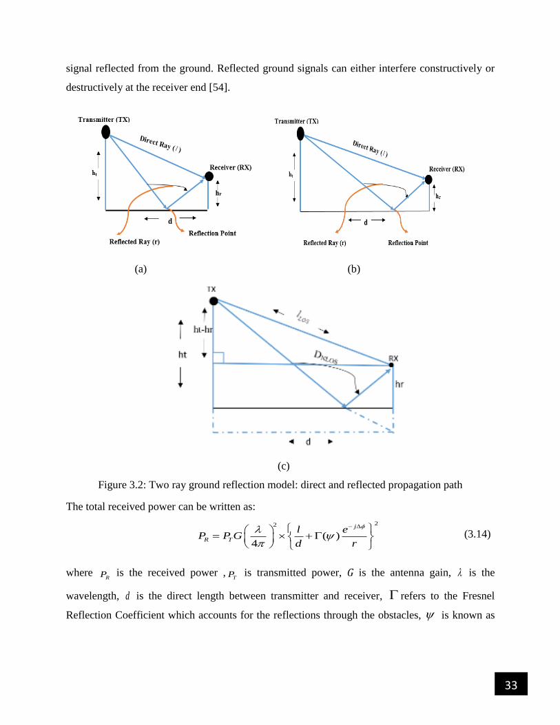
33
signal reflected from the ground. Reflected ground signals can either interfere constructively or
destructively at the receiver end [54].
(a) (b)
(c)
Figure 3.2: Two ray ground reflection model: direct and reflected propagation path
The total received power can be written as:
22
( )4
j
R T
l eP P G
d r
(3.14)
where RP is the received power ,
TP is transmitted power, 𝐺 is the antenna gain, is the
wavelength, d is the direct length between transmitter and receiver, refers to the Fresnel
Reflection Coefficient which accounts for the reflections through the obstacles, is known as
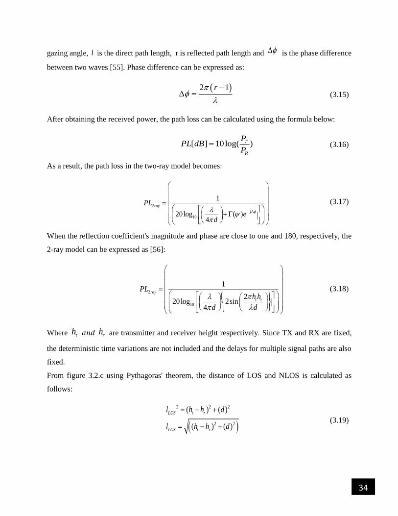
34
gazing angle, l is the direct path length, r is reflected path length and is the phase difference
between two waves [55]. Phase difference can be expressed as:
2 1r
(3.15)
After obtaining the received power, the path loss can be calculated using the formula below:
[ ] 10 log( )T
R
PPL dB
P (3.16)
As a result, the path loss in the two-ray model becomes:
2
10
1
20log ( )4
ray
j
PL
ed
(3.17)
When the reflection coefficient's magnitude and phase are close to one and 180, respectively, the
2-ray model can be expressed as [56]:
2
10
1
220log 2sin
4
ray
t r
PLh h
d d
(3.18)
Where th 𝑎𝑛𝑑 rh are transmitter and receiver height respectively. Since TX and RX are fixed,
the deterministic time variations are not included and the delays for multiple signal paths are also
fixed.
From figure 3.2.c using Pythagoras' theorem, the distance of LOS and NLOS is calculated as
follows:
2 2 2
2 2
( ) ( )
( ) ( )
LOS t r
LOS t r
l h h d
l h h d
(3.19)

35
For NLOS the path loss distance can be expressed as:
2 2 2
2 2
( ) ( )
( ) ( )
NLOS t r
LOS t r
D h h d
D h h d
(3.20)
Influence of Fresnel zone
Figure 3.2 (a) and (b) demonstrate a two-ray propagation situation. As seen in the figures, the RX
gradually travels away from the TX. When the TX moves away from the RX, the first Fresnel zone
radius increases to some point that it becomes tangent to the ground, resulting in the break point
p, which is tangent to the ground and the Fresnel zone, as shown in figure 3.3.
Figure 3.3: Two ray propagation scenario: with tangent point to the ground and Fresnel zone [57]
From the first Fresnel zone the break point distance can be expressed as [58]:
4 t r
b
h hd
(3.21)
Where th and rh are height of transmitter and receiver respectively and is wavelength.
From equation 3.20 and 3.21, the break point distance related to path loss distance is as follows:
2 2 2
2 2
2 2 2 2
2 2 2 2
( ) ( )
( ) ( ) ( )
( ) ( ) ( )
( ) 2 ( ) ( )
NLOS t r
NLOS t r r t r
NLOS t t r r t r
NLOS t t r r
D h h d
D ht h h h h h d
D h h h h h h d
D h h h h d
(3.22)
36
To relate path loss distance with break point distance, replace 2 t rh h by bd , then the equation can
be written as:
2 2 2 2( ) 2 ( ) ( )
4
* 4
NLOS t t r r
t rb
b t r
D h h h h d
h hd
d h h
(3.23)
Then divide *bd by two, the equation becomes:
*
22
bt r
dh h
(3.24)
Replace 2 t rh h by *
2
bd then, equation of the path loss distance expressed as follow:
2 2 2 2*( ) ( ) ( )
2
bNLOS t r
dD h h d
(3.25)
Where th , rh , d , bd , denotes height of transmitter, height of receiver, separation distance
between TX and RX, break point distance and wave length respectively.
By substituting equation 3.21 into equation 3.5, we derive an equation to relate the breakpoint with
path loss, as follows:
4( ) 20 log
4
4
t rb
t r
b
dPL dB
h hd
h h
d
(3.26)
Substitute in toPL , then the equation become:
( ) 20log b
t r
ddPL dB
h h
(3.27)
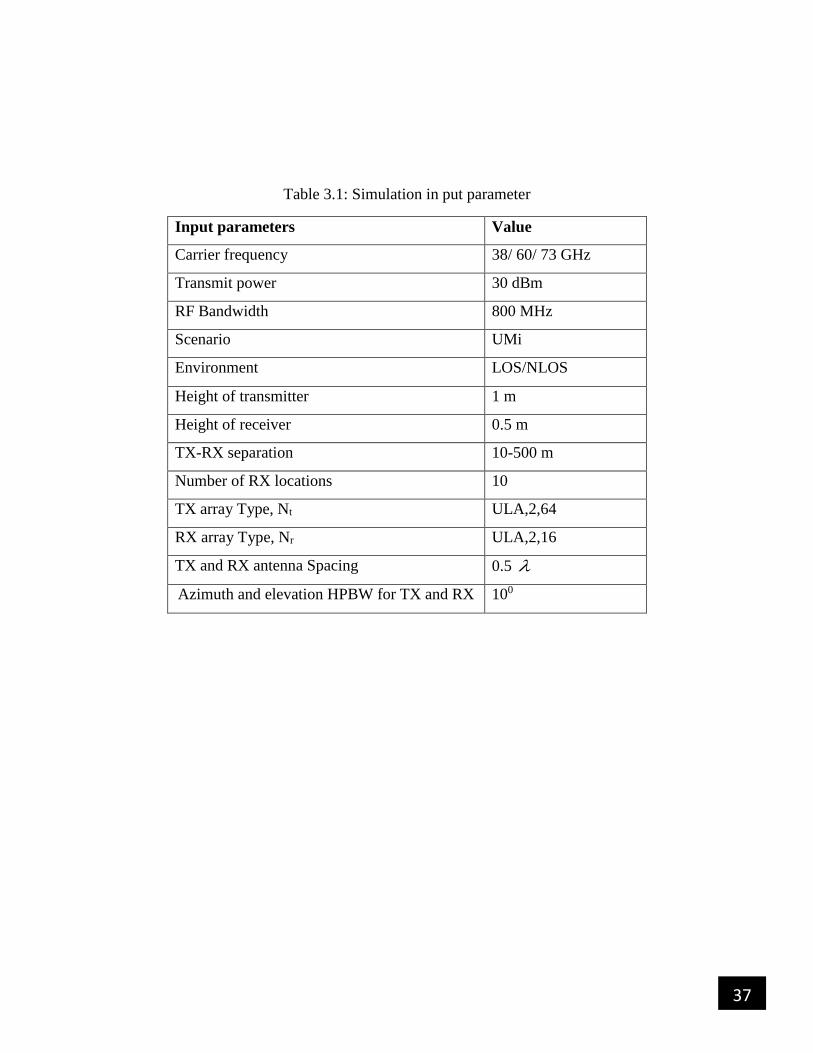
37
Table 3.1: Simulation in put parameter
Input parameters Value
Carrier frequency 38/ 60/ 73 GHz
Transmit power 30 dBm
RF Bandwidth 800 MHz
Scenario UMi
Environment LOS/NLOS
Height of transmitter 1 m
Height of receiver 0.5 m
TX-RX separation 10-500 m
Number of RX locations 10
TX array Type, Nt ULA,2,64
RX array Type, Nr ULA,2,16
TX and RX antenna Spacing 0.5
Azimuth and elevation HPBW for TX and RX 100
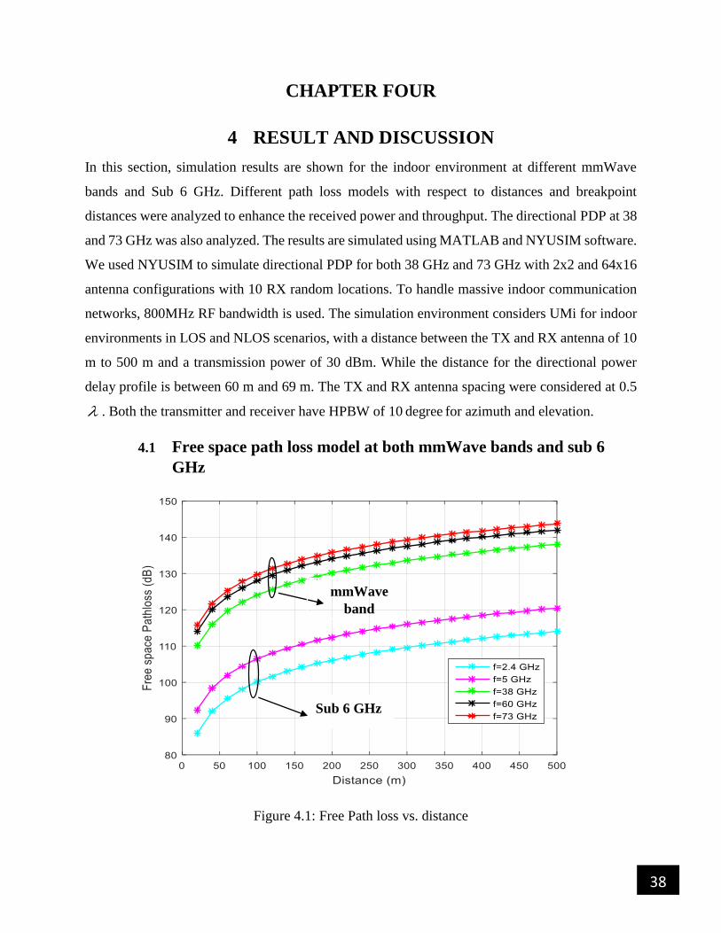
38
CHAPTER FOUR
4 RESULT AND DISCUSSION
In this section, simulation results are shown for the indoor environment at different mmWave
bands and Sub 6 GHz. Different path loss models with respect to distances and breakpoint
distances were analyzed to enhance the received power and throughput. The directional PDP at 38
and 73 GHz was also analyzed. The results are simulated using MATLAB and NYUSIM software.
We used NYUSIM to simulate directional PDP for both 38 GHz and 73 GHz with 2x2 and 64x16
antenna configurations with 10 RX random locations. To handle massive indoor communication
networks, 800MHz RF bandwidth is used. The simulation environment considers UMi for indoor
environments in LOS and NLOS scenarios, with a distance between the TX and RX antenna of 10
m to 500 m and a transmission power of 30 dBm. While the distance for the directional power
delay profile is between 60 m and 69 m. The TX and RX antenna spacing were considered at 0.5
. Both the transmitter and receiver have HPBW of 10 degree for azimuth and elevation.
4.1 Free space path loss model at both mmWave bands and sub 6
GHz
Figure 4.1: Free Path loss vs. distance
mmWave
band
Sub 6 GHz
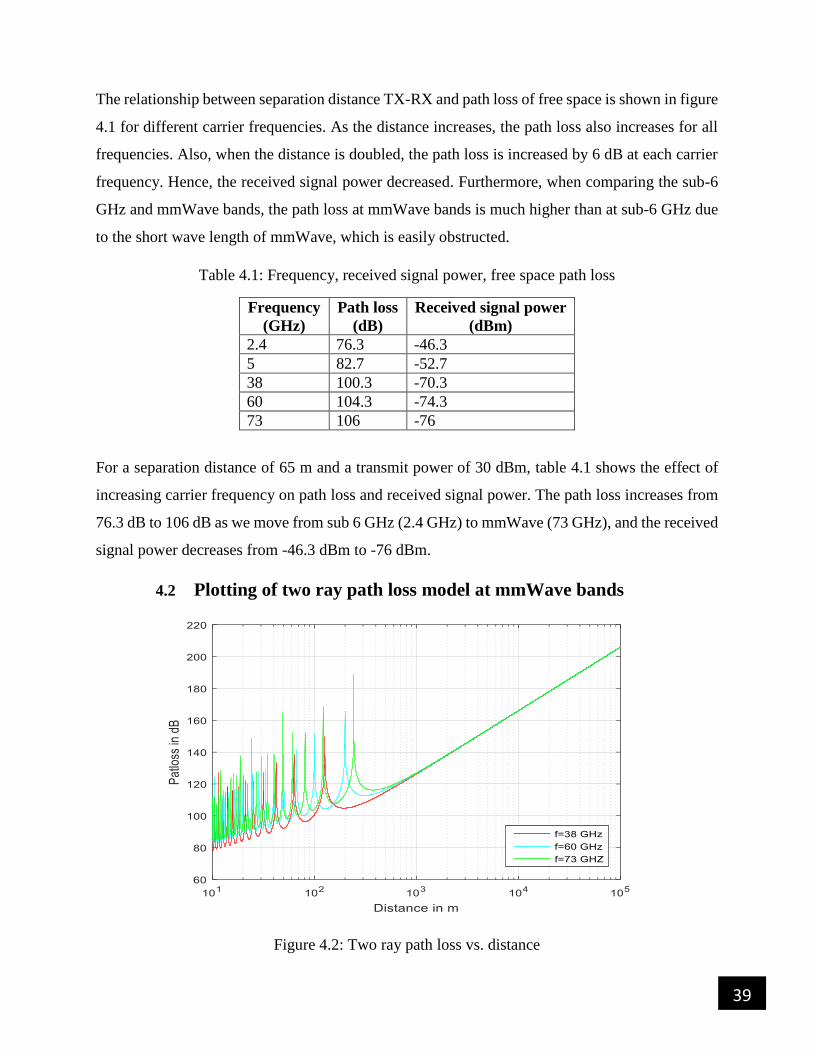
39
The relationship between separation distance TX-RX and path loss of free space is shown in figure
4.1 for different carrier frequencies. As the distance increases, the path loss also increases for all
frequencies. Also, when the distance is doubled, the path loss is increased by 6 dB at each carrier
frequency. Hence, the received signal power decreased. Furthermore, when comparing the sub-6
GHz and mmWave bands, the path loss at mmWave bands is much higher than at sub-6 GHz due
to the short wave length of mmWave, which is easily obstructed.
Table 4.1: Frequency, received signal power, free space path loss
Frequency
(GHz)
Path loss
(dB)
Received signal power
(dBm)
2.4 76.3 -46.3
5 82.7 -52.7
38 100.3 -70.3
60 104.3 -74.3
73 106 -76
For a separation distance of 65 m and a transmit power of 30 dBm, table 4.1 shows the effect of
increasing carrier frequency on path loss and received signal power. The path loss increases from
76.3 dB to 106 dB as we move from sub 6 GHz (2.4 GHz) to mmWave (73 GHz), and the received
signal power decreases from -46.3 dBm to -76 dBm.
4.2 Plotting of two ray path loss model at mmWave bands
Figure 4.2: Two ray path loss vs. distance

40
The relationship between two ray path loss with transmitter-receiver separation distance for 38,
60, and 73 GHz, with the height of the transmitter at 1m and the height of the receiver at 0.5 m, is
illustrated in figure 4.2. As the distance between the transmitter-receiver increases due to the
movement of the user away from the transmitter, the path loss in two rays increases, reducing the
received signal power for each frequency. The path loss takes the shape of a sinusoidal wave.
These waves continue until they reach a certain point. After that point, only the path loss at 73
GHz increases linearly with distance.
4.3 CI path loss model for mmWave bands and sub 6 GHz
Figure 4.3: CI path loss vs. distance
The relationship between CI path loss and distance at sub 6 GHz and mmWave frequencies is
shown in figure 4.3. When the separation distance between TX-RX increases, the CI path loss also
increases for each frequency.
Table 4.2: Frequency, received signal power, CI path loss
Frequency
(GHz)
Path loss
(dB)
Received signal power
(dBm)
2.4 259.3 -229.3
5 265.7 -235.7
38 283.3 -253.3
60 287.3 -257.3
73 289 -259

41
Table 4.1 demonstrates the effect of raising the carrier frequency from sub 6 GHz to mmWave
bands on CI path loss and received signal power for a separation distance of 65 m and a transmit
power of 30 dBm. The path loss increases from 259 dB to 289 dB as the frequency increases from
2.4 GHz to 73 GHz, whereas the received signal power decreases from -229.3 dBm to -259 dBm.
4.4 Comparing CI and free space path loss model for mmWave
bands
Figure 4.4: Path loss vs. distance for CI and free space path loss model
The path loss and distance relationships for both free space and the CI model at 38, 60, and 73
GHz are illustrated in figure 4.4. As shown in the figure, the path loss of the free space model is
lower than the CI model, because free space does not consider the effect of shadowing and
reflection. Whereas the CI model considers all shadowing and reflection effects between the
transmitter and receiver, which decrease the received signal.
CI path loss
Model
Free space
Mode

42
4.5 Plotting of free space path loss with break point distance for
different heights of transmitter
Figure 4.5: Path loss vs. break point distance
Figure 4.5 shows the relationship between free space path loss and break point distance for
different heights of transmitter at 0.5 m height of receiver and 500 m separation distance. For each
height of transmitter, the path loss increases as the break point distance increases. The term "break
point" refers to the point at which a direct signal is reflected. The path loss increases from 82.34
dB to 88.36 dB and from 112.7 to 118 dB at 15 m and 495 m break point distances, respectively,
as the transmitter height doubles. Therefore, we conclude that when the break point is near the
transmitter, the received signal power is larger than the break point at the cell edge.
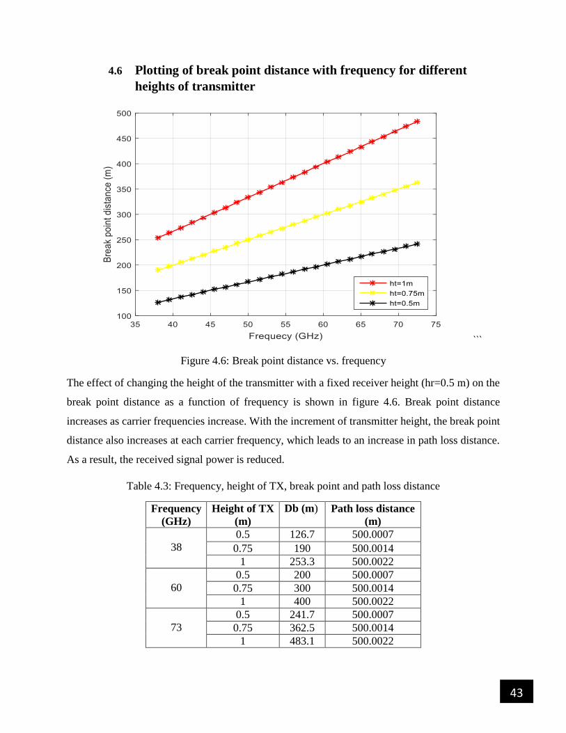
43
4.6 Plotting of break point distance with frequency for different
heights of transmitter
```
Figure 4.6: Break point distance vs. frequency
The effect of changing the height of the transmitter with a fixed receiver height (hr=0.5 m) on the
break point distance as a function of frequency is shown in figure 4.6. Break point distance
increases as carrier frequencies increase. With the increment of transmitter height, the break point
distance also increases at each carrier frequency, which leads to an increase in path loss distance.
As a result, the received signal power is reduced.
Table 4.3: Frequency, height of TX, break point and path loss distance
Frequency
(GHz)
Height of TX
(m)
Db (m) Path loss distance
(m)
38
0.5 126.7 500.0007
0.75 190 500.0014
1 253.3 500.0022
60
0.5 200 500.0007
0.75 300 500.0014
1 400 500.0022
73
0.5 241.7 500.0007
0.75 362.5 500.0014
1 483.1 500.0022

44
Table 4.3 shows the effect of transmitter height on carrier frequencies of 38, 60, and 73 GHz with
a separation distance of 500 m and a receiver height of 0.5 m. When the height of the transmitter
is increased from 0.5 to 1 meter, the break point distance doubles and the path loss distance
increases from 500.0007 to 500.0022 m for all frequencies.
Using the MATLAB-based NYUSIM simulator, we examined the directional PDP with the
strongest power at 38 and 73, using 2x2 and 64x16 antenna configurations. The impulse response
of a channel model is explained by PDP, which characterizes the channel's temporal
characteristics. Furthermore, a PDP describes how a signal is received at the receiver end with
variable signal power as it travels through a multipath channel with increasing propagation time.
4.7 Comparing directional PDP for LOS and NLOS at 28 and 73
GHz using a 2x2 antenna configuration
(a) LOS directional PDP (b) NLOS directional PDP
Figure 4.7: Directional PDP at 38 GHz for both LOS and NLOS environment with 2x2 antenna
configuration
The Directional PDP with the strongest power is illustrated in figure 4.7. The figures show the
received power vs. propagation time, as well as received signal power, path loss, PLE, RMS delay
spread, and antenna characteristics for both LOS and NLOS conditions at 38 GHz for the ULA

45
2X2 antenna configuration. As seen in figure 4.7.a, the received power decreases exponentially as
propagation time increases, and the inter-cluster gap widens. The term inter-cluster gap refers to
the short time the transmitted signal takes from reflection and scattering to reach the receiver end.
Figure 4.7.b shows received power decreasing exponentially with increasing propagation time,
similar to figure 4.7.a. Therefore, we conclude that the received power has an inverse relationship
with the propagation time for both LOS and NLOS PDPs with the strongest power. When
comparing figures 4.7.a and 4.7.b, the received power of LOS is higher than NLOS. Additionally,
the propagation time of NLOS is longer than that of LOS, as indicated in the figures.
Table 4.4: Directional power delay characteristics at 38 GHz for 2x2 antenna configuration
Frequency
(GHz)
Scenario TX-RX
Separation (m) (ns) Pr (dBm) PL
(dB)
PLE
38 LOS 66.9 0.8 -26.9 106.1 2.3
NLOS 65.6 0.6 -41.6 120.9 3.1
Table 4.4 shows power delay statistics with RMS delay spread, received power, path loss, and PLE
for both LOS and NLOS directional PDP at 38 GHz using a 2X2 antenna configuration. In the
LOS scenario, the received signal power is -26.9 dBm with PLE 2.3, whereas in NLOS it is -41.6
dBm with PLE 3.1. As a result, the received signal in the LOS scenario is larger than in the NLOS
scenario, since in the NLOS scenario, there are many obstacles between the transmitter and the
users, causing the transmitted signal to go through a multipath channel, reducing the received
signal power. Furthermore, when comparing the PLE for both LOS and NLOS scenarios to the
PLE for free space, the PLE for LOS is nearly equal to the PLE for free space, but the PLE for
NLOS is more than it.
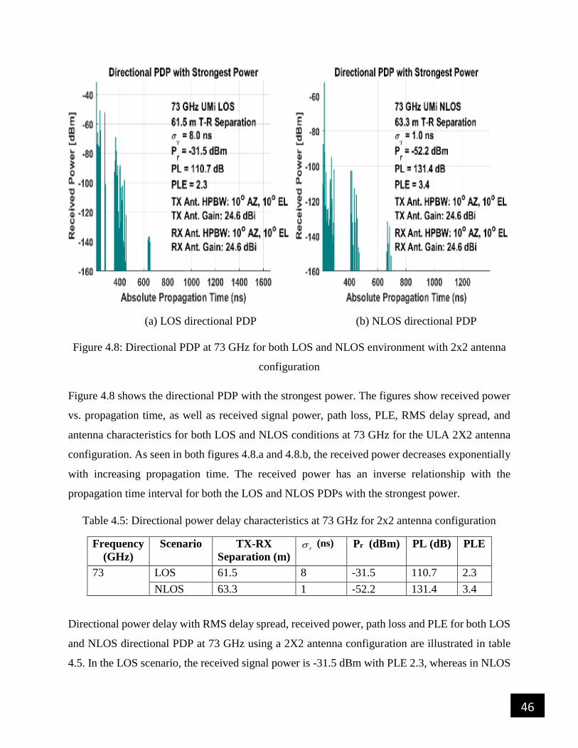
46
(a) LOS directional PDP (b) NLOS directional PDP
Figure 4.8: Directional PDP at 73 GHz for both LOS and NLOS environment with 2x2 antenna
configuration
Figure 4.8 shows the directional PDP with the strongest power. The figures show received power
vs. propagation time, as well as received signal power, path loss, PLE, RMS delay spread, and
antenna characteristics for both LOS and NLOS conditions at 73 GHz for the ULA 2X2 antenna
configuration. As seen in both figures 4.8.a and 4.8.b, the received power decreases exponentially
with increasing propagation time. The received power has an inverse relationship with the
propagation time interval for both the LOS and NLOS PDPs with the strongest power.
Table 4.5: Directional power delay characteristics at 73 GHz for 2x2 antenna configuration
Frequency
(GHz)
Scenario TX-RX
Separation (m) (ns) Pr (dBm) PL (dB) PLE
73 LOS 61.5 8 -31.5 110.7 2.3
NLOS 63.3 1 -52.2 131.4 3.4
Directional power delay with RMS delay spread, received power, path loss and PLE for both LOS
and NLOS directional PDP at 73 GHz using a 2X2 antenna configuration are illustrated in table
4.5. In the LOS scenario, the received signal power is -31.5 dBm with PLE 2.3, whereas in NLOS
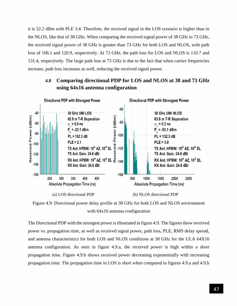
47
it is 52.2 dBm with PLE 3.4. Therefore, the received signal in the LOS scenario is higher than in
the NLOS, like that of 38 GHz. When comparing the received signal power of 38 GHz to 73 GHz,
the received signal power of 38 GHz is greater than 73 GHz for both LOS and NLOS, with path
loss of 106.1 and 120.9, respectively. At 73 GHz, the path loss for LOS and NLOS is 110.7 and
131.4, respectively. The large path loss at 73 GHz is due to the fact that when carrier frequencies
increase, path loss increases as well, reducing the received signal power.
4.8 Comparing directional PDP for LOS and NLOS at 38 and 73 GHz
using 64x16 antenna configuration
(a) LOS directional PDP (b) NLOS directional PDP
Figure 4.9: Directional power delay profile at 38 GHz for both LOS and NLOS environment
with 64x16 antenna configuration
The Directional PDP with the strongest power is illustrated in figure 4.9. The figures show received
power vs. propagation time, as well as received signal power, path loss, PLE, RMS delay spread,
and antenna characteristics for both LOS and NLOS conditions at 38 GHz for the ULA 64X16
antenna configuration. As seen in figure 4.9.a, the received power is high within a short
propagation time. Figure 4.9.b shows received power decreasing exponentially with increasing
propagation time. The propagation time in LOS is short when compared to figures 4.9.a and 4.9.b
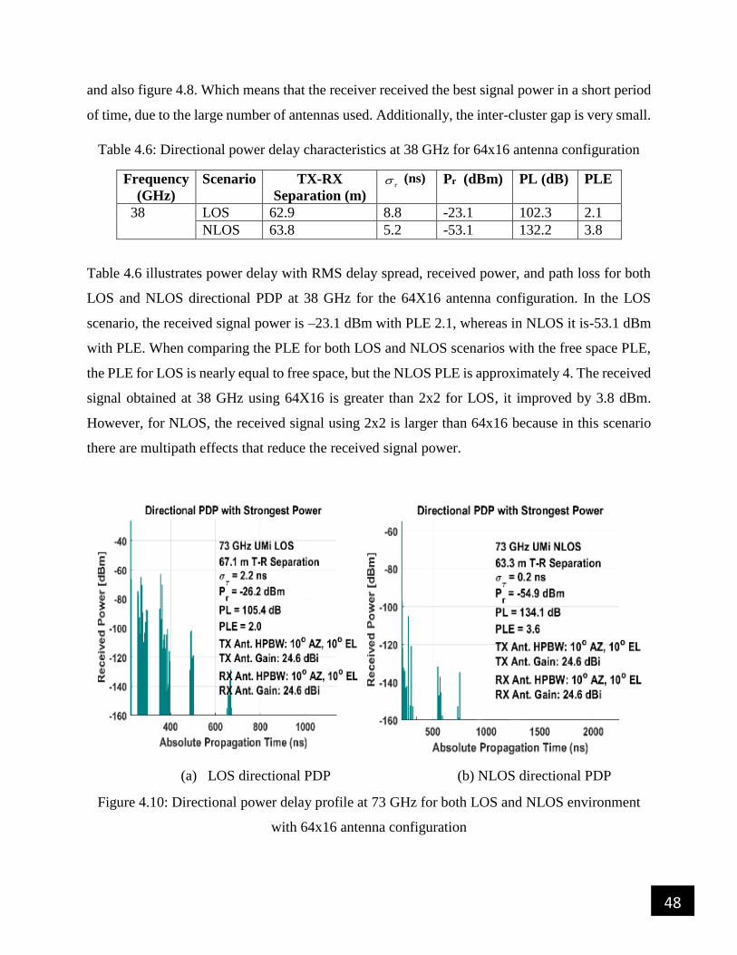
48
and also figure 4.8. Which means that the receiver received the best signal power in a short period
of time, due to the large number of antennas used. Additionally, the inter-cluster gap is very small.
Table 4.6: Directional power delay characteristics at 38 GHz for 64x16 antenna configuration
Frequency
(GHz)
Scenario TX-RX
Separation (m) (ns) Pr (dBm) PL (dB) PLE
38 LOS 62.9 8.8 -23.1 102.3 2.1
NLOS 63.8 5.2 -53.1 132.2 3.8
Table 4.6 illustrates power delay with RMS delay spread, received power, and path loss for both
LOS and NLOS directional PDP at 38 GHz for the 64X16 antenna configuration. In the LOS
scenario, the received signal power is –23.1 dBm with PLE 2.1, whereas in NLOS it is-53.1 dBm
with PLE. When comparing the PLE for both LOS and NLOS scenarios with the free space PLE,
the PLE for LOS is nearly equal to free space, but the NLOS PLE is approximately 4. The received
signal obtained at 38 GHz using 64X16 is greater than 2x2 for LOS, it improved by 3.8 dBm.
However, for NLOS, the received signal using 2x2 is larger than 64x16 because in this scenario
there are multipath effects that reduce the received signal power.
(a) LOS directional PDP (b) NLOS directional PDP
Figure 4.10: Directional power delay profile at 73 GHz for both LOS and NLOS environment
with 64x16 antenna configuration

49
The Directional PDP with the strongest power is illustrated in figure 4.10. The figures show
received power vs. propagation time, as well as received signal power, path loss, PLE, RMS delay
spread, and antenna characteristics for both LOS and NLOS conditions at 73 GHz for the ULA
64X16 antenna configuration. The received power decreases exponentially as propagation time
increases, as seen in figures 4.9.a and 4.9.b. When we compare figure 4.10.a with figure 4.10.b
and figure 4.9, the received signal power in LOS is large. Which means that the receiver received
the best signal power of the two, due to the large number of antennas used.
Table 4.7: Directional power delay characteristics at 73 GHz for 64x16 antenna configuration
Frequency
(GHz)
Scenario TX-RX
Separation (m) (ns) Pr (dBm) PL (dB) PLE
73 LOS 67.1 2.2 -26.2 105.4 2
NLOS 63.3 0.2 -54.9 134.1 3.6
Table 4.7 illustrates power delay statistics with RMS delay spread, received power, path loss, and
PLE for both LOS and NLOS for directional PDP at 73 GHz for a 64X16 antenna configuration.
In the LOS scenario, the received signal power is -26.2 dBm with PLE 2.3, whereas in NLOS it is
-54.1 dBm with PLE 3.6. When comparing the PLE for both the LOS and NLOS scenarios to the
PLE for free space, the LOS PLE equals free space, while the NLOS PLE exceeds it. The received
signal power obtained at 73 GHz using 64X16 is greater than 2x2 for LOS and improved by 5.3
dBm. However, for NLOS, the received signal using 2x2 is larger than 64x16, like that of 38 GHz.
Therefore, we conclude that increasing the number of antennas enhances the received signal power
for frequencies in LOS, whereas in the NLOS scenario, it decreases the received signal power.
50
5 CONCLUSION AND RECOMMENDATION
5.1 Conclusion
The vast amount of unused frequency resources in the mmWave spectrum is being considered as
one of the primary solutions to indoor communication network congestion. Hence, the frequency
bands in mmWave offer larger bandwidths for wireless indoor communication systems. Despite
the fact that a huge bandwidth is employed, mmWave technology suffers from path loss,
atmospheric attenuation, building penetration loss, diffuse scattering from rough materials,
shadowing, and reflection loss. As a result, the transmitted signal power and throughput are
decreased. In this thesis, path loss is considered at 38 GHz, 60 GHz, 73 GHz and sub 6 GHz using
CI, two-ray and free space path loss models.
The results have shown that the path loss increases with an increase in separation distance and
carrier frequency. The path loss in the CI model is larger than that of two rays and free space,
because it considers all the shadowing and reflection effects between transmitter and receiver.
Despite the fact of high path loss, the CI model is the most suitable for an indoor communication
network. Additionally, the relationship between breakpoint distance and path loss have been
examined. Path loss increases as the breakpoint distance and carrier frequency increase. In
addition, when the break point distance is greater than the separation distance, the PLE is larger
than in free space PLE.
Finally, the directional power delay profile with the strongest power at 38 and 73 GHz for both
LOS and NLOS environments using 2x2 and 64x16 antenna configurations has been examined. In
both antenna configurations, the received signal power in LOS at 38 GHz and 73 GHz is greater
than in NLOS. Furthermore, for both carrier frequencies, the received signal power in a 64x16
antenna configuration is larger than in a 2x2 configuration. Therefore, we conclude that increasing
the number of antennas used at the transmitter increases the received signal power and throughput.
However, increasing the number of antennas increases the received power of the LOS scenario,
not the NLOS scenario. Hence, in 64x16 for both 38 and 73 GHz in NLOS, the received power is
smaller than in the 2x2 NLOS scenario. Moreover, the PLE is nearly equal to the free space PLE
in all LOS scenarios, whereas in NLOS it is greater than in free space.
51
5.2 Recommendation
In this thesis, the performance of the CI, free space and two ray path loss models with respect to
separation distance and break point distance were analyzed. The received signal power and
throughput are enhanced by minimizing the path loss for the used carrier frequencies by using a
large number of antennas at BSs. In the future, using different polarization techniques, antenna
configurations (URA), and other techniques called beam-forming are recommended to be done to
enhance the received signal power and throughput in the given area for different mmWave
frequencies by considering other impairments of the mmWave indoor communication network.

52
REFERENCES
[1] Z. Lin, X. Du, H. Chen, B. Ai, Z. Chen, and D. Wu (2019), “Millimeter-Wave Propagation
Modeling and Measurements for 5G Mobile Networks,” no. February, pp. 72–77.
[2] M. Series (2015), “IMT Vision--Framework and overall objectives of the future
development of IMT for 2020 and beyond,” Recomm. ITU, vol. 2083.
[3] S. Mumtaz, J. Rodriguez, and L. Dai (2016), “MmWave massive MIMO: a paradigm for
5G,” Academic Press.
[4] T. E. Bogale and L. B. Le (2016), “Massive MIMO and mmWave for 5G wireless HetNet:
Potential benefits and challenges,” IEEE Veh. Technol. Mag., vol. 11, no. 1, pp. 64–75.
[5] J. G. Andrews et al. (2014), “What will 5G be?,” IEEE J. Sel. areas Commun., vol. 32, no.
6, pp. 1065–1082.
[6] Z. Pi and F. Khan (2011), “An introduction to millimeter-wave mobile broadband systems,”
IEEE Commun. Mag., vol. 49, no. 6, pp. 101–107.
[7] F. Rusek et al. (2012), “Scaling up MIMO: Opportunities and challenges with very large
arrays,” IEEE Signal Process. Mag., vol. 30, no. 1, pp. 40–60.
[8] L. Wei, R. Q. Hu, Y. Qian, and G. Wu (2014), “Key elements to enable millimeter wave
communications for 5G wireless systems,” IEEE Wirel. Commun., vol. 21, no. 6, pp. 136–
143.
[9] M. A. Mou (2019), “Indoor mmWave Statistical Channel Model at V-Band for 5G
Networks,” pp. 26–28.
[10] F. Al-Ogaili and R. M. Shubair (2016), “Millimeter-wave mobile communications for 5G:
Challenges and opportunities,” in 2016 IEEE International Symposium on Antennas and
Propagation (APSURSI), pp. 1003–1004.
[11] A. M. Al-samman, T. Abd, M. Hadri, and S. A. Al-gailani (2018), “Millimeter-wave
propagation measurements and models at 28 GHz and 38 GHz in a dining room for 5G
wireless networks,” Measurement, vol. 130, pp. 71–81.
[12] Y. Niu, Y. Li, D. Jin, L. Su, and A. V Vasilakos (2015), “A survey of millimeter wave
communications (mmWave) for 5G: opportunities and challenges,” Wirel. networks, vol.
21, no. 8, pp. 2657–2676.
[13] G. Ancans, V. Bobrovs, A. Ancans, and D. Kalibatiene (2017), “Spectrum considerations
for 5G mobile communication systems,” Procedia Comput. Sci., vol. 104, pp. 509–516.
53
[14] P. Tracy (2016), “What is Mm Wave and How Does It Fit into 5G?,” Diambil dari
http//www. rcrwireless. com/20160815/fundamentals/mmwave-5g-tag31-tag99.
[15] D. T. Jangam (2013), “Mm waves role in satellite communication,” IOSR-JECE, vol. 4, no.
4, pp. 1–4.
[16] S. Singh and M. Chawla (2017), “A Review on Millimeter Wave Communication and
Effects on 5G Systems,” Iarjset, vol. 4, no. 7, pp. 28–33.
[17] X. Ge, S. Tu, G. Mao, C.-X. Wang, and T. Han (2016), “5G ultra-dense cellular networks,”
IEEE Wirel. Commun., vol. 23, no. 1, pp. 72–79.
[18] M. Xiao et al. (2017), “Millimeter Wave Communications for Future Mobile Networks,”
IEEE J. Sel. Areas Commun., vol. 35, no. 9, pp. 1909–1935.
[19] N. K. Mallat, M. Ishtiaq, A. U. Rehman, and A. Iqbal (2020), “Millimeter-Wave in the Face
of 5G Communication Potential Applications,” IETE J. Res., vol. 0, no. 0, pp. 1–9.
[20] 5G Americas (2020) ,"Understanding mmWave Spectrum for 5G Networks [whitepaper]"
pp. 1–108.
[21] M. R. Akdeniz et al. (2014), “Millimeter wave channel modeling and cellular capacity
evaluation,” IEEE J. Sel. areas Commun., vol. 32, no. 6, pp. 1164–1179.
[22] I. A. Hemadeh, K. Satyanarayana, M. El-Hajjar, and L. Hanzo (2017), “Millimeter-wave
communications: Physical channel models, design considerations, antenna constructions,
and link-budget,” IEEE Commun. Surv. \& Tutorials, vol. 20, no. 2, pp. 870–913.
[23] T. S. Rappaport et al. (2013), “Millimeter wave mobile communications for 5G cellular: It
will work!,” IEEE access, vol. 1, pp. 335–349.
[24] Y.-P. Zhang, P. Wang, and A. Goldsmith (2015), “Rainfall effect on the performance of
millimeter-wave MIMO systems,” IEEE Trans. Wirel. Commun., vol. 14, no. 9, pp. 4857–
4866.
[25] M. Marcus and B. Pattan (2005), “Millimeter wave propagation: spectrum management
implications,” IEEE Microw. Mag., vol. 6, no. 2, pp. 54–62.
[26] T. S. Rappaport and S. Deng (2015), “73 GHz Wideband Millimeter-Wave Foliage and
Ground Reflection Measurements and Models,” pp. 1238–1243.
[27] T. S. Rappaport, R. W. Heath Jr, R. C. Daniels, and J. N. Murdock (2015), Millimeter wave
wireless communications. Pearson Education.
[28] Z. Pi and F. Khan (2011), “System design and network architecture for a millimeter-wave

54
mobile broadband (MMB) system,” in 34th IEEE Sarnoff Symposium, pp. 1–6.
[29] S. Rangan, T. S. Rappaport, and E. Erkip (2014), “Millimeter-wave cellular wireless
networks: Potentials and challenges,” Proc. IEEE, vol. 102, no. 3, pp. 366–385.
[30] A. N. Uwaechia and N. M. Mahyuddin (2020), “A comprehensive survey on millimeter
wave communications for fifth-generation wireless networks: Feasibility and challenges,”
IEEE Access, vol. 8, pp. 62367–62414.
[31] L. Raschkowski, P. Kyösti, K. Kusume, T. Jämsä, and V. Nurmela (2015), “Deliverable D1.
4: METIS channel models,” METIS, Doc. Number ICT-317669-METIS/D1. 4.
[32] R. J. Weiler et al. (2016), “Quasi-deterministic millimeter-wave channel models in
MiWEBA,” EURASIP J. Wirel. Commun. Netw., vol. 2016, no. 1, pp. 1–16.
[33] S. Jaeckel, L. Raschkowski, K. Börner, and L. Thiele, “QuaDRiGa (2014): A 3-D multi-
cell channel model with time evolution for enabling virtual field trials,” IEEE Trans.
Antennas Propag., vol. 62, no. 6, pp. 3242–3256.
[34] R. Hasan, M. M. Mowla, M. A. Rashid, M. K. Hosain, and I. Ahmad (2019), “A Statistical
Analysis of Channel Modeling for 5G mmWave Communications,” 2nd Int. Conf. Electr.
Comput. Commun. Eng. ECCE 2019, pp. 7–9.
[35] H. Shokri-Ghadikolaei, L. Gkatzikis, and C. Fischione (2015), “Beam-searching and
transmission scheduling in millimeter wave communications,” in 2015 IEEE international
conference on communications (ICC), pp. 1292–1297.
[36] W. Roh et al. (2014), “Millimeter-Wave Beamforming as an Enabling Technology for 5G
Cellular,” IEEE Commun. Mag., vol. 52, no. 2, pp. 106–113.
[37] B. Romanous, N. Bitar, A. Imran, and H. Refai (2016), “Network densification: Challenges
and opportunities in enabling 5G,” 2015 IEEE 20th Int. Work. Comput. Aided Model. Des.
Commun. Links Networks, CAMAD 2015, no. I, pp. 129–134.
[38] E. Hossain and M. Hasan (2015), “IEEE Instrumentation & Measurement Magazine 5G
Cellular: Key Enabling Technologies and Research Challenges,” IEEE Instrum. Meas.
Mag., vol. 15, no. June, pp. 11–21.
[39] C. Seker, M. T. Güneser, and T. Ozturk (2018), “A review of millimeter wave
communication for 5G,” in 2018 2nd International Symposium on Multidisciplinary Studies
and Innovative Technologies (ISMSIT), pp. 1–5.
[40] M. M. Abdulwahid, O. A. S. Al-ani, M. F. Mosleh, and R. A. Abd-alhmeed (2019),

55
“Investigation of millimeter-wave indoor propagation at different frequencies,” pp. 2–8.
[41] A. M. Al-Samman et al. (2019), “Comparative study of indoor propagation model below
and above 6 GHz for 5G wireless networks,” Electronics, vol. 8, no. 1, p. 44.
[42] O. C. Nosiri, C. F. Umanah, C. C. Otubelu, and O. O. Okechukwu (2020), “Performance
Analysis Of Millimeter-Wave Pathloss Propagation Models For 5G Network In An Indoor
Environment,” vol. 9, no. 1, pp. 32–38.
[43] G. R. Maccartney, S. Member, S. Deng, S. Member, and T. S. Rappaport (2016), “Indoor
Office Plan Environment and Layout-Based MmWave Path Loss Models for 28 GHz and
73 GHz,” pp. 0–5.
[44] D. Pimienta-del-Valle, L. Mendo, J. M. Riera, and P. Garcia-del-Pino (2020), “Indoor LOS
Propagation Measurements and Modeling at 26, 32, and 39 GHz Millimeter-Wave
Frequency Bands,” Electronics, vol. 9, no. 11, p. 1867.
[45] S. Deng, M. K. Samimi, and T. S. Rappaport (2015), “28 GHz and 73 GHz Millimeter-
Wave Indoor Propagation Measurements and Path Loss Models,” pp. 8–12.
[46] M. B. Majed, T. A. Rahman, O. A. Aziz, M. N. Hindia, and E. Hanafi (2018), “Channel
Characterization and Path Loss Modeling in Indoor Environment at 4 . 5 , 28 , and 38GHz
for 5G Cellular Networks,” vol. 2018.
[47] A. F. Molisch (2012), Wireless communications, vol. 34. John Wiley \& Sons.
[48] G. R. Maccartney, T. S. Rappaport, S. Sun, and S. Deng (2015), “Indoor office wideband
millimeter-wave propagation measurements and channel models at 28 and 73 GHz for ultra-
dense 5G wireless networks,” IEEE access, vol. 3, pp. 2388–2424.
[49] L. Rubio et al. (2019), “Contribution to the channel path loss and time-dispersion
characterization in an office environment at 26 GHz,” Electronics, vol. 8, no. 11, p. 1261.
[50] D. Pimienta-del-Valle, S. Hernández-Sáenz, P. Sáiz-Coronado, L. Mendo, P. Garcia-del-
Pino, and J. M. Riera (2019), “Indoor path loss measurements at the 5G millimeter-wave
bands of 26 and 39 GHz,” in 2019 13th European Conference on Antennas and Propagation
(EuCAP), pp. 1–5.
[51] T. S. Rappaport, G. R. Maccartney, S. Member, M. K. Samimi, S. Sun, and S. Member
(2015), “Wideband Millimeter-Wave Propagation Measurements and Channel Models for
Future Wireless Communication System Design,” vol. 6778, no. c, pp. 1–25.
[52] H. Munir, S. A. Hassan, H. Pervaiz, Q. Ni, and L. Musavian (2017), “Resource optimization
56
in multi-tier HetNets exploiting multi-slope path loss model,” IEEE Access, vol. 5, pp.
8714–8726.
[53] S. Sun, G. R. MacCartney, and T. S. Rappaport (2016), “Millimeter-wave distance-
dependent large-scale propagation measurements and path loss models for outdoor and
indoor 5G systems,” in 2016 10th European Conference on Antennas and Propagation
(EuCAP), pp. 1–5.
[54] A. Bhuvaneshwari, R. Hemalatha, and T. Satyasavithri (2015), “Path loss prediction
analysis by ray tracing approach for NLOS indoor propagation,” in 2015 International
Conference on Signal Processing and Communication Engineering Systems, pp. 486–491.
[55] N. H. Ranchagoda, S. Kandeepan, M. Ding, A. Al-Hourani, and K. M. Gomez (2019),
“Diversity Based Coverage Improvement for Air-to-Ground Wireless Channels,” in 2019
IEEE International Conference on Wireless for Space and Extreme Environments (WiSEE),
pp. 116–121.
[56] N. Mehrnia and M. K. Ozdemir (2019), “Ray tracing-based maritime channel analysis for
millimeter radiowaves,” J. Infrared, Millimeter, Terahertz Waves, vol. 40, no. 1, pp. 108–
130.
[57] R. He et al. (2012), “Analysis of the Relation Between Fresnel Zone and Path Loss
Exponent Based on Two-Ray Model,” vol. 11, pp. 208–211.
[58] E. Zochmann, K. Guan, and M. Rupp (2017), “Two-ray models in mmWave
communications,” IEEE Work. Signal Process. Adv. Wirel. Commun. SPAWC, vol. 2017-
July, pp. 1–5.

57
APPENDIX
clc; clear all; close all; c=3*10^8; hr=0.5; ht=1; hrv=1.45:.05:1.85; pt=30 axis=[]; pl11=[]; pl12=[]; pl13=[]; fsl1=[]; fsl2=[]; fsl3=[];
f=2.4*1e9 f2=5*1e9 f3=38*1e9 f4=60*1e9 f5=73*1e9 d=0:20:500 lam=c/f lam1=c/f2 lam2=c/f3 lam3=c/f4 lam4=c/f5
pl=20*log10(4*pi*d./lam) pl1=20*log10(4*pi*d./lam1) pl2=20*log10(4*pi*d./lam2) pl3=20*log10(4*pi*d./lam3) pl4=20*log10(4*pi*d./lam4)
plot(d,pl,'c-*','linewidth',1) ; hold on plot(d,pl1,'m-*','linewidth',1);hold on plot(d,pl2,'g-*','linewidth',1);hold on plot(d,pl3,'k-*','linewidth',1);hold on plot(d,pl4,'r-*','linewidth',1); xlabel('Distance (m)'); ylabel('Free space Pathloss (dB)'); legend('f=2.4 GHz','f=5 GHz','f=38 GHz', 'f=60 GHz','f=73 GHz'); grid
%--------------------------------------------- figure
for i=1000:5000 d1=10^(i/1000); axis=[axis d1]; fsl=((lam2/(4*3.14*d1))^2) fsl1=((lam3/(4*3.14*d1))^2) fsl2=((lam4/(4*3.14*d1))^2)
pl4=1/(fsl*(((2*sin(2*3.14*hr*ht/(lam2*d1)))^2)));
58
pl5=1/(fsl1*(((2*sin(2*3.14*hr*ht/(lam3*d1)))^2))); pl6=1/(fsl2*(((2*sin(2*3.14*hr*ht/(lam4*d1)))^2))); pl11=[pl11,10*log10(pl4)]; pl12=[pl12,10*log10(pl5)]; pl13=[pl13,10*log10(pl6)]; fsl1=[fsl1,10*log10(fsl)]; end semilogx(axis,pl11, 'r-',axis,pl12, 'c-',axis,pl13, 'g-') xlabel('Distance in m'); ylabel('Patloss in dB'); grid on legend('f=38 GHz','f=60 GHz ','f=73 GHZ') %--------------------------------------------- figure p_L4=32.44+20*log10(f)+10*1.7*log10(d)+1.5 p_L3=32.44+20*log10(f2)+10*1.7*log10(d)+3 p_L=32.44+20*log10(f3)+10*1.7*log10(d)+3 p_L1=32.44+20*log10(f4)+10*1.7*log10(d)+3 p_L2=32.44+20*log10(f5)+10*1.7*log10(d)+3 pl=20*log10(4*pi*d./lam2) pl1=20*log10(4*pi*d./lam3) pl2=20*log10(4*pi*d./lam4) plot(d,p_L4,'c-*','linewidth',1) ; hold on plot(d,p_L3,'g-*','linewidth',1) ; hold on plot(d,p_L,'b-*','linewidth',1) ; hold on plot(d,p_L1,'m-*','linewidth',1);hold on plot(d,p_L2,'y-*','linewidth',1);hold on
xlabel('Distance (m)'); ylabel(' CI pathloss(dB)'); legend('f=2.5 GHz','f=5 GHz','f=38 GHz','f=60 GHz','f=73 GHz'); grid %---------------------------------------------- figure plot(d,p_L,'b-*','linewidth',1) ; hold on plot(d,p_L1,'m-*','linewidth',1);hold on plot(d,p_L2,'y-*','linewidth',1);hold on
plot(d,pl,'r-o','linewidth',1) ; hold on plot(d,pl1,'k-o','linewidth',1);hold on plot(d,pl2,'c-o','linewidth',1);hold on xlabel('Distance (m)'); ylabel(' pathloss(dB)'); legend('f=38 GHz','f=60 GHz','f=73 GHz'); grid %----------------------------------------------------- figure d=500; hr1=0.5 htx=0.5 htx1=0.75 hr1=1.8 dbx=0:15:500 vv=dbx.^2 pl_db=(4*pi*d)^2.*vv/(4*ht*hr1)^2 pl_db1=(4*pi*d)^2.*vv/(4*htx1*hr1)^2 pl_db2=(4*pi*d)^2.*vv/(4*htx*hr1)^2
59
zz=10*log10(pl_db); zy=10*log10(pl_db1); zx=10*log10(pl_db2); plot(dbx,zz,'r-*','linewidth',1) ; hold on plot(dbx,zy,'b-*','linewidth',1) ; hold on plot(dbx,zx,'m-*','linewidth',1) ; hold on legend('ht=0.5','ht=0.75','ht=1') xlabel('Break point Distance (m)'); ylabel('Pathloss(dB)'); grid
%--------------------------------------------------- figure hr1=0.5 htx=0.5 htx1=0.75 f=38:1.5:73 f=f.*10^9 db=(4*ht*hr1)./(c./f) dby=(4*htx1*hr1)./(c./f) dby1=(4*htx*hr1)./(c./f) plot(f/1e9,db,'r-*','linewidth',1) ;hold on plot(f/1e9,dby,'y-*','linewidth',1) ;hold on plot(f/1e9,dby1,'k-*','linewidth',1) ; xlabel('Frequecy (GHz)'); ylabel('Break point distance (m)'); legend('ht=1','ht=0.75','ht=0.5') grid